fast and reliable anomaly detection in categorical...
TRANSCRIPT

Fast and Reliable Anomaly Detection in Categorical Data
Leman AkogluCMU, SCS
5000 Forbes AvePittsburgh PA [email protected]
Hanghang TongIBM T. J. Watson19 Skyline Drive
Hawthorne, NY [email protected]
Jilles VreekenUniversity of Antwerp
Middelheimlaan 1B2020 Antwerp, [email protected]
Christos FaloutsosCMU, SCS
5000 Forbes AvePittsburgh PA [email protected]
ABSTRACTSpotting anomalies in large multi-dimensional databases is a cru-cial task with many applications in finance, health care, secu-rity, etc. We introduce COMPREX, a new approach for identify-ing anomalies using pattern-based compression. Informally, ourmethod finds a collection of dictionaries that describe the norm ofa database succinctly, and subsequently flags those points dissimi-lar to the norm—with high compression cost—as anomalies.
Our approach exhibits four key features: 1) it is parameter-free; it builds dictionaries directly from data, and requires no user-specified parameters such as distance functions or density and sim-ilarity thresholds, 2) it is general; we show it works for a broadrange of complex databases, including graph, image and relationaldatabases that may contain both categorical and numerical features,3) it is scalable; its running time grows linearly with respect to bothdatabase size as well as number of dimensions, and 4) it is effective;experiments on a broad range of datasets show large improvementsin both compression, as well as precision in anomaly detection,outperforming its state-of-the-art competitors.
Categories and Subject DescriptorsH.2.8 [Database Applications]: Data mining; E.4 [Coding andInformation Theory]: Data compaction and compression
Keywordsanomaly detection, categorical data, data encoding
1. INTRODUCTIONDetecting anomalies and irregularities in data is an important
task, and numerous applications exist where anomaly detection isvital, e.g. detecting network intrusion, credit card fraud, insuranceclaim fraud, and so on. In addition to revealing suspicious behav-ior, anomaly detection is useful for spotting rare events such asrare diseases in medicine, in addition to data cleaning and filter-ing. Finding anomalies, however, is a difficult task, in particularfor complex multi-dimensional databases.
In this work, we address the problem of anomaly detection inmulti-dimensional categorical databases using pattern-based com-
Permission to make digital or hard copies of all or part of this work forpersonal or classroom use is granted without fee provided that copies arenot made or distributed for profit or commercial advantage and that copiesbear this notice and the full citation on the first page. To copy otherwise, torepublish, to post on servers or to redistribute to lists, requires prior specificpermission and/or a fee.CIKM’12, October 29–November 2, 2012, Maui, HI, USA.Copyright 2012 ACM 978-1-4503-1156-4/12/10 ...$10.00.
pression. Compression-based techniques have been explored mostlyin communications theory, for reduced transmission cost and in-creased throughput and in databases, for reduced storage cost andincreased query performance. Here, we improve over recent workthat identified compression as a natural tool for spotting anoma-lies [22]. Simply put, we define the norm by the patterns that com-press the data well. Then, any data point that can not be compressedwell is said not to comply with the norm, and thus is abnormal.
The heart of our method, COMPREX, is to use a set of dictionar-ies to encode a database. We exploit correlations between the fea-tures in the database, grouping those with high information gain,and build dictionaries (also look-up tables or code tables [25]) foreach group of strongly interacting features. Informally, these dic-tionaries capture the data distribution in terms of patterns; the moreoften a pattern occurs, the shorter its encoded length. The goal is tofind the optimal set of dictionaries that yield the minimal losslesscompression, and then spot tuples with long encoded lengths.
Dictionary based compression has been shown to be highly ef-fective for anomaly detection in [22], which employs the KRIMPitemset-based compressor introduced by [21]. Besides high perfor-mance, it allows for characterization: one can easily inspect how tu-ples are encoded, and hence why one is deemed an anomaly. In thispaper we show that our COMPREX can do better, yielding both bet-ter compression (and relatedly, higher detection accuracy) as wellas lower running time.
The intuition behind our method achieving better compressionis that it uses multiple code tables to describe the data, whereasKRIMP builds a single code table. As such, our method can bet-ter exploit correlations between groups of features, as by doingaway with uncorrelated features it can locally assign codes moreeffectively. Moreover, we build code tables directly from data ina bottom-up fashion, instead of filtering very large collections ofpre-mined candidate patterns, which becomes exponentially costlywith increasing database dimension, i.e. number of features.
Furthermore, by not requiring the user to provide a collection ofcandidate itemsets, nor a minimal support threshold, COMPREX isparameter free in both theory and practice. We employ the Mini-mum Description Length principle to automatically decide the num-ber of feature groups, which features to group, what patterns to in-clude in the code tables, as well as to point out anomalies. In con-trast, most existing anomaly detection methods have several param-eters, such as the choice of a similarity function, density or distancethresholds, number of nearest neighbors, etc.
In a nutshell, we improve over the state of the art by encodingdata using multiple code tables, instead of one—allowing us tobetter grasp strongly interacting features. Moreover, we build ourmodels directly from data—avoiding the expensive step of miningand filtering large collections of candidate patterns.

Experiments show the resulting models obtain high performancein anomaly detection, improving greatly over the state of the artfor categorical data. We further show COMPREX is very generallyapplicable; after discretization it matches the state of the art fornumerical data, and correctly identifies anomalies both in translatedlarge graphs and image data.
2. PRELIMINARIES AND BACKGROUNDIn this section, we give the preliminaries and notation, and intro-
duce basic concepts used throughout the paper.
2.1 PreliminariesIn this paper we consider categorical databases. A database D
is a bag of n tuples over a set of m categorical features F ={f1, . . . , fm}. Each feature f ∈ F has a domain dom(f) of pos-sible values {v1, v2, . . .}. The number of values v ∈ dom(f) isthe arity of f , i.e. arity(f) = |dom(f)| ∈ N .
The domains are distinct between features. That is, dom(fi) ∩dom(fj) = ∅, ∀i 6= j. The domain of a feature set F ⊆ F is theCartesian product of the domains of the individual features f ∈ F ,i.e., dom(F ) =
∏f∈F dom(f).
A databaseD is simply a collection of n tuples, where each tuplet is a vector of length m containing a value for each feature in F .As such, D can also be regarded as a n-by-m matrix, where thepossible values in a column i are determined by dom(fi).
An item is a feature-value pair (f = v), with f ⊆ F , andv ∈ dom(f). A itemset is then a pair (F = v), for a set of featuresF ⊆ F , and v ∈ dom(F ) is a vector of length |F |. We typicallyrefer to an itemset as a pattern .
A tuple t is said to contain a pattern (F = v), denoted as p(F =v) ⊆ t (or p ⊆ t for short), if for all features f ∈ F , tf = vfholds. The support of a pattern (F = v) is the number of tuples inD that contain it: supp(F = v) = |{t ∈ D | (F = v) ⊆ t}|. Itsfrequency is then freq(F = v) = supp(F = v)/|D|.
Finally, the entropy of a feature set F is defined as
H(F ) = −∑
v∈dom(F )
freq(F = v) log freq(F = v) .
All logarithms are to base 2, and by convention, 0 log 0 = 0.
2.2 The MDL principleThe Minimum Description Length (MDL) principle [20] is a
practical version of Kolmogorov Complexity [16], and can be re-garded as model selection based on lossless compression.
Given a set of modelsM, MDL identifies the best model M ∈M as the one that minimizes
L(M) + L(D |M) ,
in which L(M) is the length in bits of the description of the modelM , and L(D | M) is the length of the description of the dataencoded by M . That is, the MDL-optimal model for a database Dencodes D most succinctly among all possible models; it providesthe best possible lossless compression.
MDL provides us a systematic approach for selecting the modelthat best balances the complexity of the model and its fit to the data.While models that are overly complex may provide an arbitrarilygood fit to the data and thus have low L(D | M), they overfitthe data, and are penalized with a relatively high L(M). Overlysimple models, on the other hand, have very low L(M), but asthey fail to identify important structure in D, their correspondingL(D | M) tends to be relatively high. As such, the MDL-optimalmodel provides the best balance between model complexity andgoodness of fit.
2.3 Dictionary based compressionTo use MDL, we need to define what a model is, how to encode
the data with such a model, and how to encode a model.
2.3.1 Data encodingAs models, we will use code tables. A code table is a simple
two column table. The first column contains patterns, which areordered descending (1) first by length and (2) second by support.The second column contains the code words code(p) correspond-ing to each pattern p. An illustrative database with 6 tuples and anexample code table for the database is illustrated in Table 1.
Table 1: An illustrative database D and an example code tableCT for a set of three features, F={f1, f2, f3}.
Data Code Table
f1f2f3 p(F = v) code(p) usage(p) L(code(p))
a b x a b x 0 4 1 bita b x a c 10 2 2 bitsa b x x 110 1 3 bitsa b x y 111 1 3 bitsa c xa c y
The code words in the second column of a code table CT arenot important: their lengths are. The length of a code word for apattern depends on the database we want to compress. Intuitively,the more often a pattern occurs in the database, the shorter its codeshould be. The usage of a pattern p ∈ CT is the number of tuplest ∈ D which contain p in their cover, i.e. have the code of p intheir encoding.
The encoding of a tuple t, given a CT , works as follows: thepatterns in the first column are scanned in their predefined order tofind the first pattern p for which p ⊆ t. p is then said to be usedin the cover of t , and the corresponding code word for p in thesecond column becomes part of the encoding of t. If t \ p 6= ∅, theencoding continues with t \ p until t is completely covered, whichyields a unique set of patterns that form the cover of t.
Given the usages of the patterns in a CT , we can compute thelengths of the code words for the optimal prefix code [20]. Shannonentropy gives the length for the optimal prefix code for p:
L(code(p) | CT ) = − log( usage(p)∑p′∈CT
usage(p′)).
The number of bits to encode a tuple t is simply the sum of thecode lengths of the patterns in its cover, that is,
L(t | CT ) =∑
p∈cover(t)
L(code(p) | CT ).
The total length in bits of the encoded database is then the sumof the lengths of the encoded data tuples,
L(D | CT ) =∑t∈D
L(t | CT ).
2.3.2 Model encodingTo find the MDL-optimal compressor, we also need to deter-
mine the encoded size of the model, the code table in our case.Clearly, the size of the second column in a given code table CTthat contains the prefix code words code(p) is trivial; it is simplythe sum of their lengths. For the size of the first column, we needto consider all the singleton items I contained in the patterns, i.e.,I =
⋃f∈F dom(f).
For encoding the patterns in the left hand column we again usean optimal prefix code. We first compute the frequency of their ap-pearance in the first column, and then by Shannon entropy calculatethe optimal length of these codes. Specifically, the encoding of thefirst column in a code table requires cH(P ) bits, where c is the totalcount of singleton items in the patterns p ∈ CT , H(.) denotes theShannon entropy function, and P is a multinomial random variablewith the probability pi = ri
cin which ri is the number of occur-
rences of singleton item i ∈ I in the first column (for the actualitems, one could add an ASCII table providing the matching fromthe prefix codes to the original names. Since all such tables are overI, this only adds an additive constant to the total cost). All in all,
L(CT ) =∑p∈CT
L(code(p) | CT ) +∑i∈I
−ri log(pi).
3. PROPOSED METHOD
3.1 Compression with Set of Tables: TheoryIn the previous section, we showed how to encode a database
D using a single code table CT . In fact, this is the approach in-troduced in [21] to compress transaction databases, employing fre-quent itemset mining to generate the candidate patterns for the codetable. Here, we do not regard transaction data, but regular relationaldata, where tuples are data points in a multi-dimensional categor-ical feature space. In this space, some groups of features may behighly correlated; and hence may be compressed well together.
As a result we can improve by using multiple code tables—as wecan then exploit correlations, and build a separate, probably smallerCT for each highly correlated group of features instead of a single,large CT for all, possibly uncorrelated features. As such, usingmultiple, that is a set of code tables, and mining these efficiently(bypassing the costly frequent itemset mining), are two of the maincontributions of our work.
Next, we formally introduce the concept of feature partitioning,and give our problem statement.
DEFINITION 1. A feature partitioning P = {F1, . . . , Fk} of aset of features F is a grouping of F , for which (1) each partitioncontains one or more features: ∀Fi ∈ P : Fi 6= ∅, (2) all partitionsare pairwise disjoint: ∀i 6= j : Fi ∩ Fj = ∅, and (3) every featurebelongs to a partition:
⋃Fi = F .
FORMAL PROBLEM STATEMENT 1. Given a set of n data tu-ples in D over a set of m features in F , find a partitioning P :{F1, F2, . . . , Fk} of F and a set of associated code tables CT :{CTF1 , CTF2 , . . . , CTFk}, such that the total compression costin bits given below is minimized.
L(P, CT , D) = L(P) +∑F∈P
L(πF (D)|CTF ) +∑F∈P
L(CTF ) ,
in which πFi(D) is the projection of D on feature subspace Fi.
Note that the number of features m and the number of tuplesn are fixed over all models we consider for a D, and hence are aconstant additive that we can safely ignore.
3.1.1 Partition encodingThe first term of L(P, CT , D) denotes the length of encoding
the partitioning, which consists of two parts; encoding (a) the num-ber of partitions and (b) the features per partition.(a) Encoding the number of partitions: First, we need to en-code k, the number of partitions and code tables. For this, we use
the MDL-optimal encoding of an integer [12]. The cost for encod-ing an integer value k is L0(k) = log?(k) + log(c), with c =∑
2− log(n) ≈ 2.865064,, and log?(k) = log(k) + log log(k) +· · · sums over all positive terms. Note that as log(c) is constant forall models, we ignore it.(b) Encoding the features per partition: Then, for each featurewe have to describe to which partition it belongs. This we do usingm log(k) bits.
In summary, L(P) = log?(k) +m log(k).
3.1.2 Data encodingThe second term of L(P, CT , D) denotes the cost of encoding
the data with the given set of code tables. To do so, each tuple ispartitioned according to P , and encoded using the optimal codes inthe corresponding code tables following the procedure in §2.3.1.
3.1.3 Model encodingThe last term of L(P, CT , D) denotes the model cost, that is the
total length of encoding the code tables. Each code table is encodedfollowing the procedure described in §2.3.2.
We note that the number of feature groups k is not a parameter ofour method but rather is determined by MDL. In particular, MDLensures that we will not have two separate code tables for a pair ofhighly correlated feature groups as it would yield lower data cost toencode them together. On the other hand, combining feature groupsmay yield larger code tables, that is higher model cost, which maynot compensate for the savings from the data cost. In other words,we group features for which the total encoding cost L(P, CT , D)is reduced. Basically, we employ MDL to both guide us in findingwhich features to group, as well as in deciding how many groupswe should have.
Also note that compression is a type of statistical method, how-ever, instead of having to choose a prior distribution appropriate forthe data (normal, chi-square, etc.) we use a rich model class (codetables) to induce the distribution from the data.
3.2 Mining Set of Code Tables: AlgorithmHaving defined the cost function as L(P, CT , D), we need an
algorithm to search for the best set of code tables CT for the opti-mal vertical partitioning P of the data such that the total encodedsize L(P, CT , D) is minimized.
The search space for finding the best code table for a given set offeatures, yet alone for finding the optimal partitioning of features,however, is quite large. Finding the optimal code table for a set of|Fi| features involves finding all the possible patterns with differentvalue combinations up to length |Fi| and choosing a subset of thosepatterns that would yield the minimum total cost on the databaseinduced on Fi. Furthermore, the number of possible partitioning ofa set of m features is the well-known Bell number Bm.
While the search space is prohibitively large, it neither has astructure nor exhibits monotonicity properties which could help usin pruning. As a result, we resort to heuristics. Our approach buildsthe set of code tables in a greedy bottom-up, iterative fashion. Wegive the pseudo-code as Algorithm 1, and explain it in more detailin the following.
COMPREX starts with a partitioning P in which each featurebelongs to its own group (1), and separate, elementary code tablesCTi for each feature fi associated with the feature sets (2).
DEFINITION 2. An elementary code tableCT encodes a databaseD induced on a single feature f ∈ F . The patterns p ∈ CT consistof all length-1 unique items v1, . . . , varity(f) in dom(f). Finally,usage(p ∈ CT ) = freq(f = v).

Typically, some features of the data will be more strongly cor-related than others, e.g., the age of a car and its fuel efficiency, orthe weather temperature and flu outbreaks. In such cases, it will beworthwhile to represent features for which the correlation is ‘highenough’ together within oneCT , as we can then exploit correlationto save bits.
More formally, we know from Information Theory that giventwo (sets of) random variables (in our case feature groups) Fi andFj , the average number of bits we can save when compressing Fiand Fj together instead of separately, is known as their InformationGain. That is,
IG(Fi, Fj) = H(Fi) +H(Fj)−H(Fi, Fj) ≥ 0,
In fact, the IG of two (sets of) variables is always non-negative(zero when the variables are independent from each other), whichimplies that the data cost would be the smallest if all the featureswere represented by a single CT . On the other hand, our objectivefunction also includes the compression cost of the CT s.
Clearly, having one large CT over many (possibly uncorrelated)features will typically require more bits in model cost than it savesin data cost. Therefore, we can use IG to point out good mergecandidates, subsequently employing MDL to decide if the total costis reduced, and hence, whether to approve the merge or not.
The first step then is to compute the IGmatrix for all pairs of thecurrent feature sets, which is a non-negative and symmetric matrix(3). Let |Fi| denote the cardinality, i.e. the number of features inthe feature set Fi. We sort the pairs of feature sets in decreasingorder of IG-per-feature, i.e. normalized by their total cardinality,and start outer iterations to go over these pairs as the candidateCT sto be merged, say CTi and CTj (5). The starting cost costinit isset to the total cost with the initial set of CT s (6). The constructionof the new CTi|j then works as follows: we put all the existingpatterns pi,1, . . . , pi,ni and pj,1, . . . , pj,nj from both CT s into thenew CT (7). Following the convention, they are sorted first bylength (from longer to shorter) and second by usage (from higherto lower) (8). Candidate partitioning P is built by dropping featuresets Fi and Fj from P and including the concatenated set Fi|j (9).Similarly, we build a temporary code table set CT by dropping thecandidate tables CTi and CTj and adding the new CT i|j (10).
Next, we find all the unique rows of the database induced on Fi|j(11). These patterns of length (|Fi|+|Fj |) are sorted in decreasingorder of their occurrence in the database and constitute the candi-dates to be inserted into the new CT . Let pi|j,1, . . . , pi|j,ni|j de-note these patterns of the combined feature set Fi|j in their sortedorder of frequency. In our inner iterations (12), we insert these one-by-one (13), update (i.e. decrease) the usages of the existing over-lapping patterns (14), remove those patterns whose usage drops tozero (15), recompute the code word lengths with updated usages(16) and compute the total cost after each insertion. If total cost isreduced, we store the candidate partitioning P and associated setof code tables CT (18), otherwise we continue insertions (from 12)with the next candidate patterns for possible future cost reduction.
In the outer iterations, if total cost is reduced the IG between thenew feature set Fi|j and the rest are computed (22). Otherwise themerge is rejected and the candidates P and CT are discarded (24).Next the algorithm continues to search for future merges, and thesearch terminates when there are no more pairs of feature sets thatcan be merged for reduced cost. The resulting set of feature setsand their corresponding set of code tables constitute our solution.
Note that the data from which we induce code tables may includeoutliers. As by MDL we only allow patterns in our code tables thathelp compression, we are not prone to include spurious patterns.See [22] for a more complete discussion.
Algorithm 1 COMPREXInput: Database D with n tuples and m (categorical) featuresOutput: A heuristic solution to Problem Statement 1: a feature
partitioning P : {F1, . . . , Fk}, associated set of code tablesCT : {CT1, . . . , CTk}, and total encoded size L(P, CT , D)
1: P ← {F1, . . . , Fm}, Fi = {fi}, 1 ≤ i ≤ m2: CT ← {CT1, . . . , CTm}, where each CTi is elementary3: Compute IG between ∀(Fi, Fj) ∈ P , i > j4: repeat5: for each (Fi, Fj) ∈ P in decreasing normalized IG do6: Compute costinit ← L(P, CT , D)
7: Put patterns p ∈ CTi and p ∈ CTj into a new CT i|j8: Sort p ∈ CT i|j , (1) by length and (2) by usage9: P ← P\(Fi ∪ Fj) ∪ Fi|j
10: CT ← CT \(CTi ∪ CTj) ∪ CT i|j11: Find unique rows (candidate patterns) pi|j in DFi|j12: for each unique row pi|j,x in decreasing frequency do13: Insert pi|j,x to new CT i|j14: Decrease usages of overlapping patterns p ∈ CT i|j
and p ∈ cover(pi|j,x) by freq(pi|j,x)15: Remove patterns p ∈ CT i|j with usage(p)=016: Recompute L(code(p ∈ CT i|j)) with new usages17: if L(P, CT , D) < L(P, CT , D) then18: P ← P and CT ← CT19: end if20: end for21: if L(P, CT , D) < costinit then22: Compute IG between Fi|j and ∀Fx ∈ P, Fx 6= Fi|j23: else24: Discard P and CT25: end if26: end for27: until convergence, i.e. no more merges
3.3 Computational Speedup and ComplexityIn Algorithm 1, computationally most demanding steps are (1)
finding all the unique rows in the database under a particular featuresubspace when two feature sets are to be merged (11) and (2) aftereach insertion of a new pattern to the code table, finding the existingoverlapping patterns the usages of which to be decreased (14).
With a naive implementation, step (1) is performed on the flyscanning the entire database once and possibly using many linearscans and comparisons over the unique rows found so far in the pro-cess. Furthermore, step (2) requires a linear scan over the currentpatterns in the new code table CT i|j for each new insertion. Thetotal computational complexity of these linear searches dependson the database, however, with the outer and inner iteration levels(Lines 5 and 12, respectively), those may become computationallyinfeasible for very large databases.
We improve with a simple design choice. Instead of an integervector of usage per pattern in CT , we have a sparse matrix C forpatterns versus data points, the binary entries cji indicating whetherdata tuple i contains pattern j in its cover. Note that the row sumof the C matrix gives the usages of the patterns. In such a setting,step (1) (mining for candidate patterns) works as follows: Let Fiand Fj denote the feature sets to be merged. Let Ci denote theni × n patterns versus data tuples matrix for code table CTi andsimilarly Cj denote the nj × n matrix for CTj , in which ni andnj respectively denote the number of patterns each table has. Weobtain the usages for the new candidate patterns (merged unique

rows) under the merged feature subspace Fi|j by multiplying Ciand CTj into a ni × nj matrix U , which takes O(ninnj).
Next, we sort the merged patterns in decreasing order by theirusage Ux,y and insert them to CT i|j one-by-one. Note that weexploit the existing patterns in the code tables to be merged, ratherthan finding all the unique rows of the database. This way, wequickly identify good frequent candidates and consider only ninjof them. Since ni, nj � n, we practically reduce the number ofinner iterations (12) to a constant.
From here, step (2) (insertions) works as follows: Let Ux,y de-note the highest usage associated with the merged pattern pi(x)|pj(y).The insertion of pi(x)|pj(y) into the code table simply means theaddition of a new row to the Ci|j matrix (Ci|j is obtained by con-catenating the rows of Ci and Cj and reordering its rows (1) bylength and (2) by usage of the patterns it initially contains). Thenew row is then the dot product (i.e. logical AND) of row x inCi and the row y in Cj (data tuples which contain both pi(x) andpj(y) in their cover). Moreover, we decrease the usages of themerged patterns pi(x) and pj(y) by subtracting the new row fromboth of their corresponding rows. All these updates are O(n).
All in all, the inner loop (starting in 12) goes over ninj(≈constant)number of candidate patterns and each insertion takesO(n). There-fore, the inner loop takes O(n).
Next, we consider the outer loop (starting in 5), which tries tomerge pairs of code tables. In the worst case we get O(m2) trialswhen all merges are discarded. As a result the worst case complex-ity of COMPREX becomes O(m2n). In practice, however, manyfeatures are correlated and we obtain a merge at almost every step,yielding about linear complexity in both data size and dimension.
3.4 COMPREX at Work: Anomaly DetectionCompression based techniques are naturally suited for anomaly
and rare instance detection. Next we describe how we exploit ourdictionary based compression framework for this task.
In a given code table, the patterns with short code words, that isthose that have high usage, represent the patterns in the data thatcan effectively compress the majority of the data points. In otherwords, they capture the trends summarizing the norm in the data.On the other hand, the patterns with longer code words are rarelyused and thus encode the sparse regions in the data. Consequently,the data tuples in a database can be scored by their encoding costfor anomalousness.
More formally, given a set of code tables CT1, . . . , CTk foundby COMPREX, each data tuple t ∈ D can be encoded by one ormore code words from eachCTi, i = {1, . . . , k}. The correspond-ing patterns constitute the cover of t as discussed in §2.3.1. Theencoding cost of t is then considered as its anomalousness score;the higher the compression cost, the more likely it is “to arousesuspicion that it was generated by a different mechanism” [13].
score(t) = L(t|CT ) =∑F∈P
L(πF (t)|CTF )
=∑F∈P
∑p∈cover(πF (t))
L(code(p)|CTF )
Having computed the compression costs, one can sort them andreport the top k data points with the highest scores as possibleanomalies. An alternative way [22] is to determine a decision thresh-old θ and flag those points with a compression cost greater than θas anomalies. One can use the Cantelli’s Inequality [11] which pro-vides a well-founded way to determine a good value for the thresh-old θ for a given confidence level, that is, an upper bound for the
false positive rate. For generality, in our experiments we show theaccuracy at all decision thresholds.
4. EMPIRICAL STUDYIn our study, we explored the general applicability of COMPREX
by considering rich data. We experimented with many (publiclyavailable) datasets1 from diverse domains, as shown in Tables 2and 3. Other datasets we used include graph and satellite imagedatasets, which we will discuss in §4.2.3 and §4.2.4, respectively.The source code of COMPREX is available for research purposes2.
We evaluated our method with respect to four criteria: (1) com-pression cost in bits, (2) running time, (3) detection accuracy, and(4) scalability. We also compared our results with two state ofthe art methods, KRIMP [25] and LOF [4] (note that KRIMP wasshown [22] to outperform single-class classification methods, likeNNDD and SVDD, for the anomaly detection task; therefore forreasons of space we only compare to the winner). KRIMP is alsoa compression based anomaly detection method, but uses a singlecode table to encode a dataset. It performs the costly frequent item-set mining as a pre-processing step to generate candidate patternsfor the code table. LOF is a density-based outlier detection methodthat computes the local-outlier-factor of data points with respect totheir nearest neighbors. Neither LOF nor KRIMP are parameter-free, they respectively require the minimum support threshold andthe number of neighbors to be considered. COMPREX, in contrast,automatically determines the number of necessary code tables, aswell as which patterns to include, and as such has no parameters.
4.1 Compression cost and Running timeOne goal of our study is to develop a fast method that would
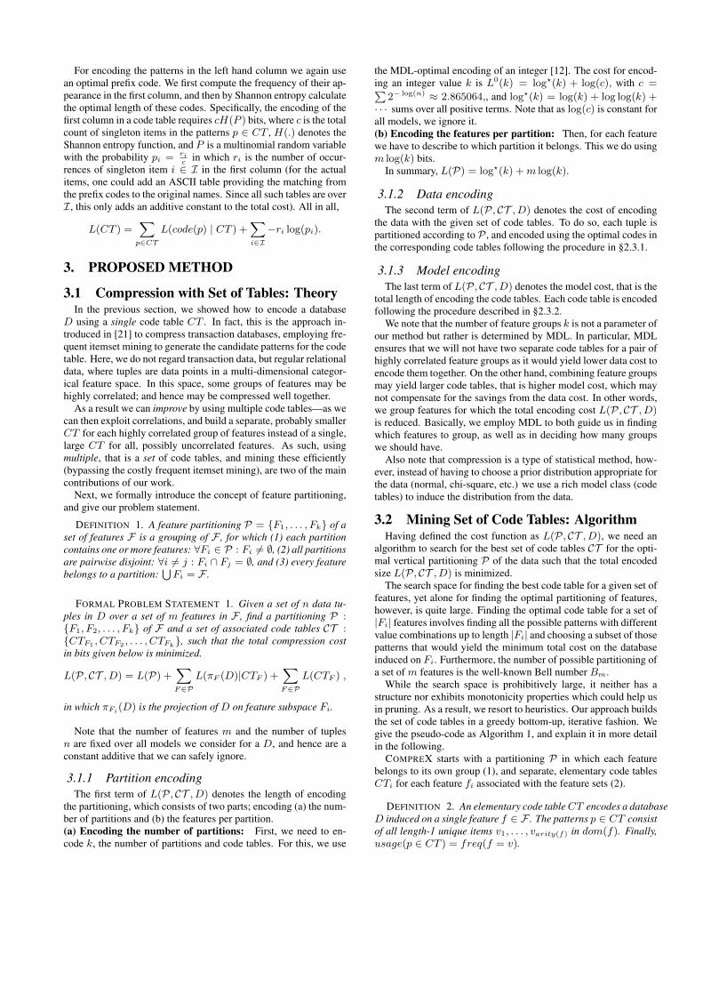
model the norm of the data and hence give low compression costin bits. In this section, we use both COMPREX and KRIMP forcompressing our datasets and show the total cost in bits and thecorresponding running times in Figure 1 (a) and (b), respectively.Note that the results for our largest datasets Enron, Connect-4, andCovertype are given with broken y-axes with values in millions forcost and thousands for time.
We note that COMPREX achieves very nice compression rates,outperforming KRIMP for all of the datasets, and providing up to96% savings in bits (47% on average).
With respect to running time, we notice that for most of the(smaller) datasets, our running time is only slightly higher thanthat of KRIMP but still remains under 16 seconds. Even thoughfor small datasets the run time of KRIMP is negligible, for datasetsespecially with large number of features, its running time increasessignificantly. The computationally most demanding part of KRIMPis the frequent itemset mining, making it less feasible for largeand high dimensional categorical datasets. For example, for theConnect-4 dataset with 42 features and the Chess (king,rook vs.king,pawn) datasets with 36 features, KRIMP cannot finish withinreasonable time due to very large candidate sets.
To alleviate this problem, KRIMP accepts a minsup parameter,which is the minimum number of occurrences of an itemset in thedatabase to be considered as frequent. The higher the minsup isset, the fewer the extracted itemsets are. However, high minsupcomes with a trade-off; the higher the minsup, the smaller the num-ber of candidates, the smaller the search space and the worse thefinal code table approximates the optimal code table. In contrast,
1http://archive.ics.uci.edu/ml/datasets.html2http://dl.dropbox.com/u/17337370/CompreX_12_tbox.tar.gz
0
100000
200000
300000
400000
500000
600000
Compression cost in bits
CompreX Krimp Original data
900000
9000000
90000000
1
2
4
8
16
32
64
128
Running time in seconds
CompreX Krimp
300 800
1300 1800 2300
Figure 1: (left) Compression cost (in bits) when encoded by COMPREX vs. KRIMP. (right) Run time (in seconds) of COMPREX vs.KRIMP. For large datasets, extremely many frequent itemsets negatively affect the runtime for KRIMP.
our method does not require any sorts of parameters and frequentitemset mining.
In our experiments, we find closed frequent itemsets with minsupset to 5000 and 500 for the Connect-4 and Chess (kr-kp) datasets,respectively. Even then, the running time of our method remainslower than that of KRIMP (see Fig. 1). On the other hand, the timerequired for frequent itemset mining also depends on the datasetcharacteristics. For example, we observe in Figure 1 that the run-ning time of KRIMP on the (larger) Mushroom dataset is muchsmaller than that on the (smaller) Spect-heart dataset, with bothhaving the same number of (22) features.
For our largest datasets (in terms of size and number of features)in Figure 1, notice that the running time of KRIMP is quite large(about 20 mins) for Enron and Connect-4, and (45 mins) for Cover-type. Moreover, its compression cost is still higher than that ourmethod provides. Therefore, we conclude that our method becomesmore advantageous especially for large datasets.
4.2 Detection accuracyBesides achieving high compression rate, we would also (if not
more) want our method to be effective in spotting anomalies. Inthis section, we experiment with various types of data includingrelational, graph and image databases.
For measuring detection performance, we use two-class datasets.The number of data points from one class is significantly smallerthan that from the other class. We call these classes as minorityand the majority classes, respectively. The data points from theminority class are considered to be the “anomalies”. The underly-ing assumption is that different classes have different distributions–some classes may be more similar than others, just like with realanomaly(-classes). Examples to the classes include poisonous vs.edible in Mushroom data, unaccountable vs. very good in Car data,and win vs. loss in Connect-4 data.
As a measure of accuracy, we use average precision; the aver-age of the precision values obtained across recall levels. We plotthe detection precision, that is the ratio of the number of true pos-itives to the total number of predicted positives, against the recall(=detection rate), that is the fraction of total true anomalies thatare detected. A point on the plot is obtained by setting a thresholdcompression cost—any record with a cost larger than that thresholdis flagged as an anomaly. The corresponding precision and recallare then calculated. By varying the threshold, we obtain the curvefor the entire range of recalls. The average precision then approxi-mates the area under the precision-recall curve.
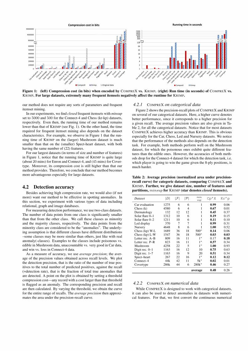
4.2.1 COMPREX on categorical dataFigure 2 shows the precision-recall plots of COMPREX and KRIMP
on several of our categorical datasets. Here, a higher curve denotesbetter performance, since it corresponds to a higher precision fora given recall. The average precision values are also given in Ta-ble 2, for all the categorical datasets. Notice that for most datasetsCOMPREX achieves higher accuracy than KRIMP. This is obviousespecially for the Car, Chess, Led and Nursery datasets. We noticethat the performance of the methods also depends on the detectiontask. For example, both methods perform well on the Mushroomdataset, for which the poisonous ones exhibit quite different fea-tures than the edible ones. However, the accuracies of both meth-ods drop for the Connect-4 dataset for which the detection task, i.e.which player is going to win the game given the 8-ply positions, ismuch harder.
Table 2: Average precision (normalized area under precision-recall curve) for categoric datasets, comparing COMPREX andKRIMP. Further, we give dataset size, number of features andpartitions, minsup for KRIMP (star denotes closed itemsets).
Dataset |D| |F| |P| minsup
Cp’X Kr’p
Car evaluation 1275 6 6 1 0.99 0.06Chess (k) 4580 6 4 1 0.67 0.01Dermatology 132 12 12 1 0.45 0.37Solar flare 0–1 1312 10 6 1 0.19 0.15Solar flare 0–2 1211 10 6 1 0.11 0.10Led display 370 7 7 1 0.99 0.31Nursery 4648 8 6 1 1.00 0.52Chess (kp) W-L 1689 36 18 500∗ 0.14 0.06Chess (kp) L-W 1547 36 18 500∗ 0.03 0.03Letter rec. A–B 809 16 11 1∗ 0.17 0.18Letter rec. P–R 823 16 11 1∗ 0.57 0.34Mushroom 4258 22 5 1∗ 1.00 0.93Digit rec. 0–1 1163 16 12 10 0.75 0.63Digit rec. 1–7 1163 16 9 20 0.51 0.34Spect–heart 267 22 16 1∗ 0.12 0.12Connect–4 44k 42 11 5k∗ 0.02 0.01Covertype 286k 44 6 280k∗ 0.46 0.27
average 0.48 0.26
4.2.2 COMPREX on numerical dataWhile COMPREX is designed to work with categorical datasets,
it can also be used to detect anomalies in datasets with numeri-cal features. For that, we first convert the continuous numerical

0 0.2 0.4 0.6 0.8 10
0.2
0.4
0.6
0.8
1
Detection rate/Recall
Det
ectio
n pr
ecis
ion
CAR
CompreX: 0.9957
KRIMP: 0.0628
0 0.2 0.4 0.6 0.8 10
0.2
0.4
0.6
0.8
1
Detection rate/Recall
Det
ectio
n pr
ecis
ion
CHESS
CompreX: 0.6782
KRIMP: 0.0044
0 0.2 0.4 0.6 0.8 10
0.2
0.4
0.6
0.8
1
Detection rate/Recall
Det
ectio
n pr
ecis
ion
DERMATOLOGY
CompreX: 0.4552
KRIMP: 0.379
0 0.2 0.4 0.6 0.8 10
0.2
0.4
0.6
0.8
1
Detection rate/Recall
Det
ectio
n pr
ecis
ion
FLARE 0−2
CompreX: 0.112
KRIMP: 0.1001
0 0.2 0.4 0.6 0.8 10
0.2
0.4
0.6
0.8
1
Detection rate/Recall
Det
ectio
n pr
ecis
ion
LED
CompreX: 0.9973
KRIMP: 0.3185
(a) Car evaluation (b) Chess (kr-k) (c) Dermatology (d) Solar flare 0-2 (e) Led display
0 0.2 0.4 0.6 0.8 10
0.2
0.4
0.6
0.8
1
Detection rate/Recall
Det
ectio
n pr
ecis
ion
NURSERY
CompreX: 1
KRIMP: 0.528
0 0.2 0.4 0.6 0.8 10
0.2
0.4
0.6
0.8
1
Detection rate/Recall
Det
ectio
n pr
ecis
ion
CHESS KR−KP
CompreX: 0.149
KRIMP: 0.063
0 0.2 0.4 0.6 0.8 10
0.2
0.4
0.6
0.8
1
Detection rate/Recall
Det
ectio
n pr
ecis
ion
LETTERS P,R
CompreX: 0.5739
KRIMP: 0.3412
0 0.2 0.4 0.6 0.8 10
0.2
0.4
0.6
0.8
1
Detection rate/Recall
Det
ectio
n pr
ecis
ion
DIGITS 0,1
CompreX: 0.7533KRIMP: 0.6383
0 0.2 0.4 0.6 0.8 10
0.2
0.4
0.6
0.8
1
Detection rate/Recall
Det
ectio
n pr
ecis
ion
COVERTYPE
CompreX: 0.467
KRIMP: 0.2783
(f) Nursery (g) Chess (kr-kp) (h) Letters P-R (i) Digits 0-1 (j) Covertype
Figure 2: Performance of COMPREX vs KRIMP on two-class categorical datasets. Given are precision vs. recall for various thresholdsto flag tuples as anomalous. Note that COMPREX outperforms KRIMP for most detection tasks.
0 0.2 0.4 0.6 0.8 10
0.2
0.4
0.6
0.8
1
Detection rate/Recall
Det
ectio
n pr
ecis
ion
SHUTTLE
CompreX: 0.9151
KRIMP: 0.063
0 0.2 0.4 0.6 0.8 10
0.2
0.4
0.6
0.8
1
Detection rate/Recall
Det
ectio
n pr
ecis
ion
SHUTTLE
CompreX: 0.8734
KRIMP: 0.39880 0.2 0.4 0.6 0.8 1
0
0.2
0.4
0.6
0.8
1
Detection rate/Recall
Det
ectio
n pr
ecis
ion
SHUTTLE
CompreX: 0.9151
KRIMP: 0.017
0 0.2 0.4 0.6 0.8 10
0.2
0.4
0.6
0.8
1
Detection rate/Recall
Det
ectio
n pr
ecis
ion
SHUTTLE
CompreX: 1
KRIMP: 0.2256
0 0.2 0.4 0.6 0.8 10
0.2
0.4
0.6
0.8
1
Detection rate/Recall
Det
ectio
n pr
ecis
ion
SHUTTLE
CompreX: 1
KRIMP: 0.0654
(a) LOG-bins (b) 5-LINbins (c) 10-LINbins (d) 3-SAXbins (e) p0.01-MDLbins
Figure 3: Performance of COMPREX vs KRIMP on the two-class numerical transaction dataset Shuttle. Notice that COMPREXoutperforms KRIMP consistently for various discretization methods used.
features to discretized nominal features. There exist various tech-niques to this end. In our study, we consider several: linear, loga-rithmic, SAX [17], and MDL-based [14] binning. Linear binninginvolves dividing the value range of each feature into equal sizedintervals. Logarithmic binning first sorts the feature values and as-signs the lower b-fraction to the first bin, the next b-fraction of therest to the second bin, and so on, until all the values are assignedto a bin. SAX has proved to be an effective symbolic represen-tation, especially for time series data. MDL-based binning esti-mates variable-width histograms with optimal bin count automati-cally, for a given data precision.
We experiment with these various discretization methods undervarious parameter settings. In Figure 3, we show the accuracy ofCOMPREX versus KRIMP on the Shuttle dataset, using logarithmicbinning with b=0.5, linear binning with 5 and 10 bins, SAX with3 bins, and MDL-based binning with precision 0.01. Results aresimilar for many other settings and for the rest of the numericaldatasets, which we omit for brevity. Notice that regardless of thediscretization used, COMPREX performs consistently better thanits competitor KRIMP.
To this end, we also compare our method with LOF on severalnumerical datasets. LOF is a widely used outlier detection methodbased on local density estimation. While it is quite powerful whenapplied to numeric data, it cannot be directly applied to categori-cal datasets. In this comparison, both methods require the carefulchoice of a parameter; number of nearest neighbors k for LOF, anda binning method and its corresponding parameter for COMPREX.
In Figure 4, we show the accuracy of LOF versus COMPREXwith their best parameter choices on our numerical two-class datasets.
Table 3: Average precision for the numerical datasets, compar-ing COMPREX, KRIMP and LOF. Further, dataset size, numberof features and partitions, minsup used for KRIMP.
Dataset |D| |F| |P| minsup
Cp’X Kr’p LOF
Shuttle 3416 9 5 1 1.00 0.22 0.83Pageblocks 4941 10 6 1 0.46 0.37 0.23Yeast 468 8 8 1 0.49 0.17 0.48Abalone 703 7 3 1 0.42 0.15 0.24
average 0.59 0.23 0.45
Table 3 gives the corresponding average precision scores for allthree methods. Notice that COMPREX achieves comparable or bet-ter performance than LOF, even though it operates on discretizeddata which loses some information due to this process, and thus isnot as optimized as LOF for numeric data. This shows that COM-PREX can also be applied to datasets with numerical or with a hy-brid of both categorical and numerical features.
4.2.3 COMPREX on graph dataGiven data points and their features in numerical or categorical
space, our method can also be applied to other complex data, in-cluding graphs. To this end, we study the Enron graph3, in whichnodes represent individuals and the edges represent email interac-tions. In our setting the nodes correspond to the data points, andthe features to the ego-net features we extract from each node. The
3http://www.cs.cmu.edu/~enron/

0 0.2 0.4 0.6 0.8 10
0.2
0.4
0.6
0.8
1
Detection rate/Recall
Det
ectio
n pr
ecis
ion
SHUTTLE
CompreX: 1LOF: 0.8302
0 0.2 0.4 0.6 0.8 10
0.2
0.4
0.6
0.8
1
Detection rate/Recall
Det
ectio
n pr
ecis
ion
PAGEBLOCKS
CompreX: 0.4624
LOF: 0.2289
0 0.2 0.4 0.6 0.8 10
0.2
0.4
0.6
0.8
1
Detection rate/Recall
Det
ectio
n pr
ecis
ion
YEAST
CompreX: 0.4895
LOF: 0.4805
0 0.2 0.4 0.6 0.8 10
0.2
0.4
0.6
0.8
1
Detection rate/Recall
Det
ectio
n pr
ecis
ion
ABALONE
CompreX: 0.4167
LOF: 0.2408
(a) Shuttle (b) Page blocks (c) Yeast (d) Abalone
Figure 4: Performance of LOF vs COMPREX with the best choice of parameters on the numerical transaction datasets. Notice thatCOMPREX achieves comparable or better performance than LOF even after discretization.
ego-net of a node (ego) is defined as the subgraph of the node, itsneighbors, and all the links between them. We extract 14 numericalego-net features, such as the number of edges, total weight, ego-netdegree (number of edges connecting the ego-net to the rest of thegraph), in- and out-degree, etc. We refer the reader to [2] for moreon ego-net features. Features are discretized into 10 linear bins.
In Table 4, we show the top 5 email addresses with the highestcompression cost found by COMPREX. The dataset does not con-tain any ground truth anomalies, therefore we provide anecdotalevidence for the discovered “anomalies”. Our first observation isthe significantly high compression cost of the listed points—103 to107 bits given a global average of 6.72 bits (median is 4.27). Thisis due to the rare and high number of patterns used in their cover.Notice that each of them are covered with 7 patterns compared toa global average of 2.05 (median is 2). Moreover, the usages ofthe cover patterns is quite small—thus longer code words and hightotal compress-cost. Further inspection justifies our results: for ex-ample, ‘sally.beck’ (employee chief operating officer) contains thehighest number of (31k) edges in its ego-net and the highest ego-net degree (of 85k), implying that she is highly connected to therest of the graph as opposed to many other nodes in the graph.
Table 4: Top-5 anomalies for Enron, with one regular-joeexample. Given are, email address, compression cost, size ofcover, and average usages of the cover patterns; high usagescorrespond to short codes. Average cost is 6.72 bits, averagenumber of covering patterns is 2.05.
[email protected] cost (bits) |cover| avg usage±stdof cover patterns
sally.beck 107.28 7 3.7 ± 5.4jeff.dasovich 107.11 7 3.4 ± 3.9outlook.team 106.70 7 4.8 ± 6.3david.forster 105.11 7 4.1 ± 5.2kenneth.lay 103.24 7 5.8 ± 7.5
......
......
robert.badeer 1.53 2 52k ± 4.3k
4.2.4 COMPREX on image dataNext, for our image datasets4 for which class labels also do not
exist, we provide an anecdotal and visual study. The image datasetsare the satellite images of four major cities from around the worldas shown in Figure 5. Each image is split into 25x25 rectangle tiles,for which we extracted 15 numerical features, and subsequentlydiscretized into 10 linear bins. The first three features denote themean RGB values for each tile and the rest denote Gabor features.
4http://geoeye.com/CorpSite/gallery/
In Figure 5, top tiles with high compression cost are highlightedin red. We observe that COMPREX effectively spots interesting andrare regions. For example, the districts of Roman Catholic Churchin Vatican and the Washington Memorial in Washington D.C. thatdistinctively stand out in the images are captured in top anomalies.In Forbidden city, COMPREX spots the three lakes (Beihai, Zhong-hai, Nanhai), the Jingshan Park on its right, as well as the Tianan-men Square on the south. Finally, in London COMPREX marks thepart of Thames river, the Buckingham Palace as well as several rareplain fields in the city.
(a) Holy see, Vatican (b) Washington D.C., USA
(c) Forbidden city, Beijing (d) London, UK
Figure 5: “Anomalous” tiles—with high compression cost—on the image datasets are highlighted with red borders (figuresbest viewed in color). Notice that COMPREX successfully spotsqualitatively distinct regions that stand out in the images.
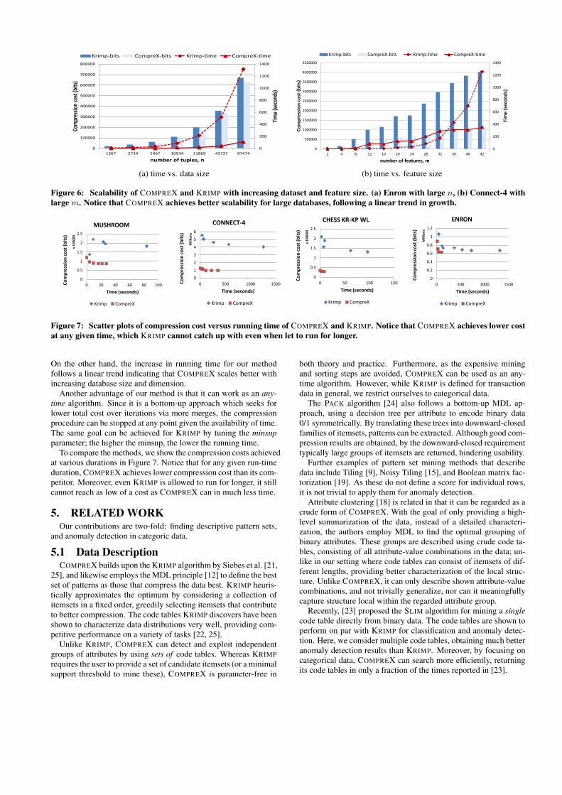
4.3 ScalabilityKRIMP falling short on large datasets arises the question of scala-
bility, which is maybe even more important than the issue of speed.Therefore, in Figure 6, we also show the running time of both meth-ods for growing dataset and feature sizes on Enron and Connect-4.
We observe that the running time of KRIMP grows significantlywith the increasing size in both cases. The difference is evidentespecially for growing feature size. This is due to frequent itemsetmining scaling exponentially with respect to number of features.
0
200
400
600
800
1000
1200
1400
0
100000
200000
300000
400000
500000
600000
700000
800000
1367 2734 5467 10934 21869 43737 87474
Tim
e (s
econ
ds)
Com
pres
sion
cos
t (bi
ts)
number of tuples, n
Krimp-bits CompreX-bits Krimp-time CompreX-time
0
200
400
600
800
1000
1200
1400
0
500000
1000000
1500000
2000000
2500000
3000000
3500000
4000000
4500000
2 4 8 12 16 20 24 28 32 36 40 42
Tim
e (
seco
nd
s)
Co
mp
ress
ion
co
st (
bit
s)
number of features, m
Krimp-bits CompreX-bits Krimp-time CompreX-time
(a) time vs. data size (b) time vs. feature size
Figure 6: Scalability of COMPREX and KRIMP with increasing dataset and feature size. (a) Enron with large n, (b) Connect-4 withlarge m. Notice that COMPREX achieves better scalability for large databases, following a linear trend in growth.
0
0.1
0.2
0.3
0.4
0.5
0 20 40 60
Co
mp
ress
ion
co
st (
bit
s)
x 1
00
00
0
Time (seconds)
PENDIGITS 0 vs. 1
Krimp CompreX
0
0.1
0.2
0.3
0.4
0.5
0 20 40 60 80
Co
mp
ress
ion
co
st (
bit
s)
x 1
00
00
0
Time (seconds)
LETTERS A vs. B
Krimp CompreX
0
0.05
0.1
0.15
0.2
0 50 100 150
Co
mp
ress
ion
co
st (
bit
s)
x 1
00
00
0
Time (seconds)
SPECT-HEART
Krimp CompreX
0
0.5
1
1.5
2
2.5
0 20 40 60 80 100 Co
mp
ress
ion
co
st (
bit
s)
x 1
00
00
0
Time (seconds)
MUSHROOM
Krimp CompreX
0
1
2
3
4
5
6
0 500 1000 1500 Co
mp
ress
ion
co
st (
bit
s)
Mill
ion
s
Time (seconds)
CONNECT-4
Krimp CompreX
0
0.5
1
1.5
2
2.5
0 50 100 150
Co
mp
ress
ion
co
st (
bit
s)
x 1
00
00
0
Time (seconds)
CHESS KR-KP WL
Krimp CompreX
0
0.5
1
1.5
2
2.5
0 100 200 300 400 500 Co
mp
ress
ion
co
st (
bit
s)
x 1
00
00
0
Time (seconds)
CHESS KR-KP LW
Krimp CompreX
0
0.2
0.4
0.6
0.8
1
1.2
0 500 1000 1500
Co
mp
ress
ion
co
st (
bit
s)
Mill
ion
s
Time (seconds)
ENRON
Krimp CompreX
0
1
2
3
4
5
6
0 500 1000 1500 Co
mp
ress
ion
co
st (
bit
s)
Mill
ion
s
Time (seconds)
CONNECT-4
Krimp CompreX
0
0.5
1
1.5
2
2.5
0 50 100 150
Co
mp
ress
ion
co
st (
bit
s)
x 1
00
00
0
Time (seconds)
CHESS KR-KP WL
Krimp CompreX
0
0.5
1
1.5
2
2.5
0 100 200 300 400 500 Co
mp
ress
ion
co
st (
bit
s)
x 1
00
00
0
Time (seconds)
CHESS KR-KP LW
Krimp CompreX
0
0.2
0.4
0.6
0.8
1
1.2
0 500 1000 1500
Co
mp
ress
ion
co
st (
bit
s)
Mill
ion
s
Time (seconds)
ENRON
Krimp CompreX
Figure 7: Scatter plots of compression cost versus running time of COMPREX and KRIMP. Notice that COMPREX achieves lower costat any given time, which KRIMP cannot catch up with even when let to run for longer.
On the other hand, the increase in running time for our methodfollows a linear trend indicating that COMPREX scales better withincreasing database size and dimension.
Another advantage of our method is that it can work as an any-time algorithm. Since it is a bottom-up approach which seeks forlower total cost over iterations via more merges, the compressionprocedure can be stopped at any point given the availability of time.The same goal can be achieved for KRIMP by tuning the minsupparameter; the higher the minsup, the lower the running time.
To compare the methods, we show the compression costs achievedat various durations in Figure 7. Notice that for any given run-timeduration, COMPREX achieves lower compression cost than its com-petitor. Moreover, even KRIMP is allowed to run for longer, it stillcannot reach as low of a cost as COMPREX can in much less time.
5. RELATED WORKOur contributions are two-fold: finding descriptive pattern sets,
and anomaly detection in categoric data.
5.1 Data DescriptionCOMPREX builds upon the KRIMP algorithm by Siebes et al. [21,
25], and likewise employs the MDL principle [12] to define the bestset of patterns as those that compress the data best. KRIMP heuris-tically approximates the optimum by considering a collection ofitemsets in a fixed order, greedily selecting itemsets that contributeto better compression. The code tables KRIMP discovers have beenshown to characterize data distributions very well, providing com-petitive performance on a variety of tasks [22, 25].
Unlike KRIMP, COMPREX can detect and exploit independentgroups of attributes by using sets of code tables. Whereas KRIMPrequires the user to provide a set of candidate itemsets (or a minimalsupport threshold to mine these), COMPREX is parameter-free in
both theory and practice. Furthermore, as the expensive miningand sorting steps are avoided, COMPREX can be used as an any-time algorithm. However, while KRIMP is defined for transactiondata in general, we restrict ourselves to categorical data.
The PACK algorithm [24] also follows a bottom-up MDL ap-proach, using a decision tree per attribute to encode binary data0/1 symmetrically. By translating these trees into downward-closedfamilies of itemsets, patterns can be extracted. Although good com-pression results are obtained, by the downward-closed requirementtypically large groups of itemsets are returned, hindering usability.
Further examples of pattern set mining methods that describedata include Tiling [9], Noisy Tiling [15], and Boolean matrix fac-torization [19]. As these do not define a score for individual rows,it is not trivial to apply them for anomaly detection.
Attribute clustering [18] is related in that it can be regarded as acrude form of COMPREX. With the goal of only providing a high-level summarization of the data, instead of a detailed characteri-zation, the authors employ MDL to find the optimal grouping ofbinary attributes. These groups are described using crude code ta-bles, consisting of all attribute-value combinations in the data; un-like in our setting where code tables can consist of itemsets of dif-ferent lengths, providing better characterization of the local struc-ture. Unlike COMPREX, it can only describe shown attribute-valuecombinations, and not trivially generalize, nor can it meaningfullycapture structure local within the regarded attribute group.
Recently, [23] proposed the SLIM algorithm for mining a singlecode table directly from binary data. The code tables are shown toperform on par with KRIMP for classification and anomaly detec-tion. Here, we consider multiple code tables, obtaining much betteranomaly detection results than KRIMP. Moreover, by focusing oncategorical data, COMPREX can search more efficiently, returningits code tables in only a fraction of the times reported in [23].

5.2 Anomaly DetectionIdentifying outliers in multi-dimensional real-valued data has been
studied extensively. Examples of proposals to this end include [1, 3,4, 7, 10]. These typically exploit the (continuous) ordered domainsof the attributes to define meaningful distance functions betweentuples, which cannot be straightforwardly applied on nominal (cat-egorical) data. Furthermore, most of these methods require severalparameters to be specified by the user. For example, [4] and [10]take the number of nearest neighbors k to be compared to as input.They also require a distance metric for finding the k-nns of thedata points, which often suffers from the curse of dimensionalityin high dimensions. Lastly, these methods do not build a model,and thus cannot provide anomaly characterization. Model-basedapproaches like COMPREX, on the other hand, capture the norm ofthe data and can pindown the deviations from it, providing betterinterpretability for the claimed anomalies.
While most work on outlier detection has focused on numeri-cal datasets, there also exist some work on anomaly detection fordiscrete data. [6] surveys methods for finding the anomalous se-quences in a given set of sequences. The main disadvantage of themethods therein (kernel-,window-based, etc.) is that their perfor-mance is highly reliant on the choice of their parameters (similaritymeasure, window size, etc.). Proposals for anomaly detection incategorical data include [5, 8, 26] and recently [22]. [5] learns astructure and the parameters of a Bayesian network, and uses thelog-likelihood values as the anomalousness score of each record.[8, 26] address the problem of finding anomaly patterns. Theybuild a Bayes net that represents the baseline distribution, and thenscore the rules with unusual proportions compared to the baseline.They restrict their method to work with only one and two compo-nent rules due to high computation required. COMPREX is mostrelated to [22], which employs KRIMP [21] as its compressor foranomaly detection. The key differences are that KRIMP finds asingle code table, performs costly frequent itemset mining for can-didate generation, and requires a minimum support parameter.
6. CONCLUSIONSThe contributions of this work are two-fold: (1) we achieve fast
characterization of data by mining subspace code-tables, i.e. pat-terns sets, and (2) we apply our descriptive patterns to reliableanomaly detection in categorical data.
We introduce a novel, parameter-free method, COMPREX, thatbuilds a data compression model using multiple dictionaries forencoding, and reports the data points with high encoding cost asanomalous. Our method proves effective for both tasks: It pro-vides higher compression rates at lower run times especially forlarge datasets, and it is capable of spotting rare instances effec-tively, with detection accuracy often higher than its state-of-the-artcompetitors. Experiments on diverse datasets show that COMPREXsuccessfully generalizes to a broad range of datasets including im-age, graph, and relational databases with both categorical and nu-merical features. Finally our method is scalable, with running timegrowing linearly with increasing database size and dimension.
Future work can generalize our method to time-evolving data fordetecting anomalies over time, where the challenge is to efficientlyupdate the code tables to effectively capture the trending patterns.
AcknowledgementResearch was sponsored by NSF under Grant No. IIS1017415, ARL un-der Coop. Agreement No. W911NF-09-2-0053, and ADAMS programsponsored by DARPA under Agreements No. W911NF-11-C-0200 andW911NF-11-C-0088. Jilles Vreeken is supported by a Post-Doctoral Fel-lowship of the Research Foundation – Flanders (FWO).
7. REFERENCES[1] C. C. Aggarwal and P. S. Yu. Outlier detection for high
dimensional data. In SIGMOD, 2001.[2] L. Akoglu, M. McGlohon, and C. Faloutsos. Oddball:
Spotting anomalies in weighted graphs. In PAKDD, 2010.[3] A. Arning, R. Agrawal, and P. Raghavan. A linear method
for deviation detection in large databases. In KDD, 1996.[4] M. M. Breunig, H. Kriegel, R. T. Ng, and J. Sander. LOF:
Identifying density-based local outliers. In SIGMOD, 2000.[5] A. Bronstein, J. Das, M. Duro, R. Friedrich, G. Kleyner,
M. Mueller, S. Singhal, and I. Cohen. Using bayes-nets fordetecting anomalies in Internet services. In INM, 2001.
[6] V. Chandola, A. Banerjee, and V. Kumar. Anomaly detectionfor discrete sequences: A survey. IEEE Trans. Knowl. DataEng., 24(5):823–839, 2012.
[7] A. Chaudhary, A. S. Szalay, and A. W. Moore. Very fastoutlier detection in large multidimensional data sets. InDMKD, 2002.
[8] K. Das and J. G. Schneider. Detecting anomalous records incategorical datasets. In KDD, 2007.
[9] F. Geerts, B. Goethals, and T. Mielikäinen. Tiling databases.In DS, pages 278–289, 2004.
[10] A. Ghoting, S. Parthasarathy, and M. E. Otey. Fast mining ofdistance-based outliers in high-dimensional datasets. DataMin. Knowl. Discov., 16(3):349–364, 2008.
[11] G. Grimmett and D. Stirzaker. Probability and RandomProcesses. Oxford University Press, 2001.
[12] P. Grünwald. The Minimum Description Length Principle.MIT Press, 2007.
[13] D. Hawkins. Identification of outliers. Chapman and Hall,1980.
[14] P. Kontkanen and P. Myllymäki. MDL histogram densityestimation. In AISTAT, 2007.
[15] K.-N. Kontonasios and T. De Bie. An information-theoreticapproach to finding noisy tiles in binary databases. In SDM,2010.
[16] M. Li and P. Vitányi. An Introduction to KolmogorovComplexity and its Applications. Springer, 1993.
[17] J. Lin, E. J. Keogh, S. Lonardi, and B. Y. Chiu. A symbolicrepresentation of time series, with implications for streamingalgorithms. In DMKD, pages 2–11, 2003.
[18] M. Mampaey and J. Vreeken. Summarising categorical databy clustering attributes. Data Min. Knowl. Disc., 2012.
[19] P. Miettinen, T. Mielikäinen, A. Gionis, G. Das, andH. Mannila. The discrete basis problem. IEEE TKDE,20(10):1348–1362, 2008.
[20] J. Rissanen. Modeling by shortest data description.Automatica, 14(1):465–471, 1978.
[21] A. Siebes, J. Vreeken, and M. van Leeuwen. Item sets thatcompress. In SDM, pages 393–404. SIAM, 2006.
[22] K. Smets and J. Vreeken. The odd one out: Identifying andcharacterising anomalies. In SDM, pages x–y. SIAM, 2011.
[23] K. Smets and J. Vreeken. SLIM: Directly mining descriptivepatterns. In SDM, pages 1–12. SIAM, 2012.
[24] N. Tatti and J. Vreeken. Finding good itemsets by packingdata. In ICDM, pages 588–597, 2008.
[25] J. Vreeken, M. van Leeuwen, and A. Siebes. KRIMP: Miningitemsets that compress. DAMI, 23(1):169–214, 2011.
[26] W.-K. Wong, A. W. Moore, G. F. Cooper, and M. M.Wagner. Bayesian network anomaly pattern detection fordisease outbreaks. In ICML, 2003.