Fast and Accurate Simulation of

Installed Antenna Performance

Matt Miller

President

September 17, 2014

Installed Antenna Performance Problem

• Antennas interact with installed platform – Multipath, diffraction, creeping waves, etc.

• Need to accurately characterize antenna performance – Communications links, radar, cosite, etc.

• Measurement vs. Simulation – Measurement is expensive, time consuming and difficult

– Simulation is affordable, fast, and flexible

Savant Overview

• Advanced installed antenna performance simulation

software

– Fast and accurate prediction of installed patterns, near-

fields, and antenna coupling

Savant Advantages

• Extremely Fast – Multicore, GPU and MPI

• Low Memory Requirements – Most jobs require less than 8 GB of RAM

• Accurate – Physics models not found in other SBR tools

• Intuitive – Powerful GUI with thorough Help/Tutorials

• Workflow – Antenna design tools, CEM tools and Matlab

• Expertise – The most experienced SBR development

team anywhere

GPU and MPI Examples

• Monopole on 737-800 – Compute installed pattern

• 40,000 angular samples

• 3 to 4 GHz, 40 MHz steps

• 747,820 rays hit CAD

– Using single CPU core: 12 hrs, 18 min

– Using four CPU cores: 3 hrs, 12 min (4x)

– Using 1 CPU core, 1 GPU: 10.7 min (> 70x)

– Using 4 CPU cores, 2 GPU: 6.2 min (>118x)

• 94 GHz Antenna on UH-60 – Compute installed pattern

– Using 1 Node, 6 cores, 2 GPUs

• 720 seconds (12 minutes)

– Using 5 Nodes, 30 CPU cores, 10 GPUs

• 143 seconds (5x)

– Computer hardware costs $20K

6,170 λ

477λ x 527λ x 167λ

Methodology: SBR+

• What is SBR ?

– SBR = Shooting and Bouncing Rays

• Asymptotic technique for electrically large platforms

• Complimentary capability to full-wave solvers

• Extends physical optics (PO) to multiple bounces with GO ray tracing

• SBR+ ?

– Build on SBR with additional physics

• Physical Theory of Diffraction (PTD)

• Creeping Wave

• Uniform Theory of Diffraction (UTD) Rays

– Driving development philosophy

• Use full array of GTD/UTD methods to “paint”

currents on platform body

• All models/mechanisms should work together

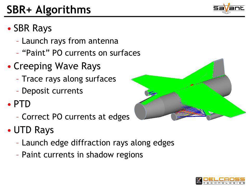
SBR+ Algorithms

• SBR Rays

– Launch rays from antenna

– “Paint” PO currents on surfaces

SBR+ Algorithms

• SBR Rays

– Launch rays from antenna

– “Paint” PO currents on surfaces

• Creeping Wave Rays

– Trace rays along surfaces

– Deposit currents

SBR+ Algorithms

• SBR Rays

– Launch rays from antenna

– “Paint” PO currents on surfaces

• Creeping Wave Rays

– Trace rays along surfaces

– Deposit currents

• PTD

– Correct PO currents at edges

SBR+ Algorithms

• SBR Rays

– Launch rays from antenna

– “Paint” PO currents on surfaces

• Creeping Wave Rays

– Trace rays along surfaces

– Deposit currents

• PTD

– Correct PO currents at edges

• UTD Rays

– Launch edge diffraction rays along edges

– Paint currents in shadow regions

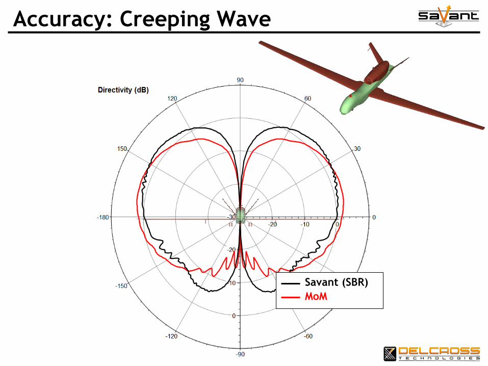
Accuracy: Creeping Wave

1 GHz monopole mounted on Global Hawk

Accuracy: Creeping Wave

SBR Rays

1 GHz monopole mounted on Global Hawk

Accuracy: Creeping Wave

Savant (SBR)

MoM

Accuracy: Creeping Wave

Creeping-wave Rays

SBR Rays

+

1 GHz monopole mounted on Global Hawk

Accuracy: Creeping Wave

Savant (SBR+CW)

MoM

Accuracy: Creeping Wave

Savant (SBR+CW)

MoM

Creeping Wave Is Very Important For This

Problem!

Savant is the only SBR tool with this

capability

UTD Edge Diffraction Rays Example

1 GHz monopole

Without UTD Rays

UTD Edge Diffraction Rays Example

1 GHz monopole

With UTD Rays

Antenna Models

• Free-space antenna model required for Savant

– Far-field radiation patterns

– Current sources

• Built in parametric models

– Dipoles, monopoles, loops, slots

– Pyramidal and Conical horns

– Parametric Beam

• Array Design Tool

– Linear, Rectangular, Elliptical & By File

– Weighting and phasing of elements

– Far-field or current sources for elements

• Import Full-Wave 3D Antenna Models

– HFSS

– CST

– FEKO

– WIPL-D

V-22 S-Band Antenna Example

S-Band Blade Antenna

2.3 GHz

1,620 simulations to

capture moving blades and

engine assemblies

6 hours to compute all

jobs on laptop 133λ x 200λ x 51λ

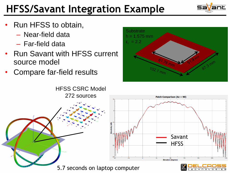
HFSS/Savant Integration Example

Substrate

h = 1.575 mm

εr = 2.2

• Run HFSS to obtain,

– Near-field data

– Far-field data

• Run Savant with HFSS current source model

• Compare far-field results

Savant

HFSS

HFSS CSRC Model

272 sources

5.7 seconds on laptop computer

HFSS/Savant Integration Example

SBR

+ Creeping Wave

250 MHz Monopole

42λ x 17λ x 3.75λ

HFSS/Savant Integration Example

Savant Runtime: 16 minutes on laptop with quad core CPU and NVIDIA Quadro

K2000M GPU

Connected Vehicle Scenario #1

• Compute installed pattern for 5.9 GHz antenna as a large

delivery truck passes the sedan

• Pattern computed every 0.1 meter as delivery truck

approaches sedan from behind and passes

251 simulations

12.5 hours to run all jobs

on laptop computer

180 seconds per simulation

651λ x 180λ x 74λ

Connected Vehicle Scenario #2

• Compute coupling between two 5.9 GHz antennas

5.9 GHz Transmitter

and Antenna

Receiver

and Antenna 287 simulations

12.1 hours to run all jobs

on laptop computer

152 seconds per simulation

651λ x 180λ x 74λ

Summary

• Savant solves enormous, realistic problems, many which you

may have considered too big to solve before

• Savant is FAST, on hardware you likely already have

• Savant plugs into a workflow with other commercial software

tools