Farther on down the road: transport costs, trade and urbangrowth in sub-Saharan Africa

Adam Storeygard∗

April 2012

Abstract

How does isolation affect the economic activity of cities? Transport costs arewidely considered an important barrier to local economic activity but their impactin developing countries is not well-studied. This paper investigates the role of inter-city transport costs in determining the income of sub-Saharan African cities. Inparticular, focusing on fifteen countries whose largest city is a port, I ask how im-portant access to that city is for the income of hinterland cities. The lack of paneldata on both local economic activity and transport costs has prevented rigorous em-pirical investigation of this question. I fill this gap with two new datasets. Satellitedata on lights at night proxy for city economic activity, and new road network dataallow me to calculate the shortest route between cities. Cost per unit distance isidentified by plausibly exogenous world oil prices. The results show that an oil priceincrease of the magnitude experienced between 2002 and 2008 induces the incomeof cities near a major port to increase by six percent relative to otherwise identicalcities one standard deviation farther away. Combined with external estimates, thisimplies an elasticity of city economic activity with respect to transport costs of -0.2at that distance. Moreover, the effect differs by the surface of roads between cities.Cities connected to the port by paved roads are chiefly affected by transport coststo the port, while cities connected to the port by unpaved roads are more affectedby connections to secondary centers.

JEL classification: F15, O18, R11, R12, R4Keywords: Urbanization, Transport costs, Infrastructure, Roads, Sub-Saharan Africa

∗Department of Economics, Brown University. Email: adam storeygard@brown.edu. I am grate-ful to David Weil, Nate Baum-Snow, and especially Vernon Henderson for their advice and support.I thank Katherine Casey, Uwe Deichmann, Leo Feler, Andrew Foster, Delia Furtado, Jake Goldston,Walker Hanlon, Erik Hurst, Blaise Melly, Sriniketh Nagavarapu, Mark Roberts, Nathan Schiff, MichaelSuher, Ishani Tewari, Matt Turner, Nicholas Wilson, Junfu Zhang, and seminar participants at Brown,CIESIN, Columbia, Georgia State, Maryland, MIT, Notre Dame, NYU, Syracuse, Toronto, Tufts, UCIrvine, Wharton, EconCon, the Midwest International Economic Development Conference, and the an-nual meetings of the Center for the Study of African Economies (CSAE) and the North American RegionalScience Council (NARSC), for helpful comments and suggestions, Uwe Deichmann and Siobhan Murrayfor access to and guidance on the roads data and NARSC and the World Bank’s Research Support Budgetand Knowledge for Change Program for funding. All errors are my own.

1 Introduction

Sub-Saharan Africa has experienced substantial economic growth in the past decade, after

a quarter century of stagnation and contraction.1 It is perhaps too early to answer the

question of why this period of growth has arrived. However, it is important to know where

it has happened within countries and why these places have been favored.

In this paper, I argue that changes in transport costs have played a critical role in

determining the growth of cities. Sub-Saharan Africa has notoriously high transport costs

compared to other major regions of the world. Population density is relatively low, with

a substantial fraction of people residing far from the coast. Ocean-navigable rivers, which

provide transport to the interior of most other regions, are virtually non-existent. And

road networks are sparse and poorly maintained, on the whole. I ask whether periphery

cities with lower transport costs to their country’s main port grew faster than those

farther away or with poorer road connections, in the context of dramatically rising oil

prices over the 2000s decade. A typical problem with testing this kind of question in

poor countries is that relevant data on cities and transport costs do not exist. This paper

provides novel measures of both. First, night time lights satellite data (Elvidge et al., 1997;

Henderson, Storeygard and Weil, 2012) are used to construct a 17-year annual panel of

city-level measures of economic activity for 287 cities in 15 countries. Second, a new set of

roads data provides information about route length and surface material. Transport costs

are thus identified by the interaction between world oil prices and distance along these

routes. Because I have data on many cities per country over a substantial time period, I

can control for annual shocks separately for each country, as well as initial characteristics

and growth rates of individual cities.

Focusing on countries whose largest, or primate, city is also a port, I find that as the

price of oil increases from $25 to $97 (as it did between 2002 and 2008), if city A is 465

kilometers (1 standard deviation) farther away from the primate than initially identical

city B, its economy is roughly 6 percent smaller than city B’s at the end of the period. At

a differential of 2360 kilometers, the largest in the data, this rises to 32 percent. Further

evidence shows that this effect is due to transport costs, not commodity income or the

generation of electricity. I then determine that this effect falls disproportionately on cities

that are connected to the primate by paved roads, most likely because they are initially

more engaged in trade. Cities connected to the primate by unpaved roads appear to be

more affected by transport costs to secondary cities. This suggests a funneling of trade

1This paper generally defines sub-Saharan Africa as all countries of the African mainland with noMediterranean coastline, plus Madagascar.

1

to small cities through nearby secondary cities, though no direct data on intercity trade

is available.

The majority of Africa’s population growth is expected to be in cities over the next

few decades (National Research Council, 2003). Indeed, of the approximately 2.5 billion

net gain in global population expected by 2050, over 30 percent is expected to be in

African cities (United Nations, 2008). Much less is understood, however, about which

cities will experience the bulk of that growth. This is the first paper that has the data

to systematically address the economic growth of cities in sub-Saharan Africa. Which

cities grow and which do not will have major implications for the future of the region.

If growth is concentrated in large coastal cities, agglomeration economies may improve,

but urban infrastructure needs, congestion, and the risks associated with sea level rise

will all increase. Many countries have pursued decentralization policies at least in part

because of these concerns. If growth is more balanced across a large group of cities,

intercity infrastructure may be more important. If cities near international borders grow

more than others, they may affect international migration and trade.2 Regional cities

that grow enough may become political power bases constituted along social or industrial

lines.

Despite a great deal of attention paid to the largest cities like Lagos, Kinshasa and

Nairobi, 61 percent of African urban residents lived in cities with a population of less than

500,000 as of 2000, and this percentage is expected to remain high over the next couple of

decades. Only 15 percent are expected to live in cities of more than one million by 2015

(National Research Council, 2003). There are only 5 out of 43 sub-Saharan countries

(Liberia, South Africa, Togo, and both Congos) in which the majority of 2005 urban

residents were in urban agglomerations with a 2007 population of more than 750,000.3 In

most countries, smaller cities are also growing faster (United Nations, 2008).

These large cities may however have greater importance to national economies than

their populations alone suggest. In many countries, a large city or core region, often a

port, plays a very important role in the economy, as the largest domestic market, the

chief manufacturing center, the primary trading connection with the rest of the world,

and the seat of elites and often of the government. Ports have a special role because most

African trade is transoceanic. Trade among the contiguous eight members of the West

African Economic and Monetary Union (WAEMU) represented less than 3 percent of

2The center of some ten sub-Saharan African capital cities is within 20 km by land of an internationalborder. Such proximity is extremely rare in other regions, except among countries less than 40 km indiameter. In six of these cases, the built-up area of the city directly abuts the border or border-river.More than half the countries in the region have capitals within 100 km of a border by air.

3All country counts were conducted prior to the independence of South Sudan.

2

their total trade for each year in the 1990s (Coulibaly and Fontagne, 2006).4 If anything,

one would expect more trade among these countries than other sets of neighbors, because

they share a common currency and thus lack one important trade friction. Other cities

in the periphery have relationships with their country’s core that are potentially critical

to their success. And countries spend to improve those links or simply to reverse decay.

Almost $7 billion is invested per year on roads in sub-Saharan Africa, with a substantial

portion funded by donors (World Bank, 2010). Worldwide, transport accounts for 15 to

20 percent of World Bank lending, with almost three quarters of that amount going to

roads (World Bank, 2007a).

This paper relates primarily to four bodies of work. The first is on the effect of

transport costs on the size and growth of cities and regions. This work has been done

primarily using cross-country data (e.g. Limao and Venables, 2001) or the construction of

very large national transport networks in the United States (Baum-Snow, 2007; Chandra

and Thompson, 2000; Atack, Bateman, Haines and Margo, 2010; Duranton and Turner,

2011), India (Donaldson, 2010), and China (Banerjee, Duflo and Qian, 2009). However,

no comparable work has been done in sub-Saharan Africa, which has worse roads, lower

urbanization, lower income, and much less industry, and consists of many countries, as

opposed to one unitary state.5 Similarly ambitious transport infrastructure projects have

not been carried out in post-independence sub-Saharan Africa. This paper instead relies

on the plausibly exogenous annual changes in transport costs induced by world oil price

fluctuations, which allow me to determine the short run impact of shocks better than

previous work. This does not mean that the changes were small, however, as average

annual oil prices varied by a nominal factor of 7.6 during the period of study (1992–

2008).6 These shocks are also of interest because they are more likely to be repeated in

the future.

The second related literature is on the scope and drivers of urbanization and urban

economic growth in Africa. This literature is almost exclusively cross-country in nature,

so that unobserved country-level factors may be confounding results (Fay and Opal, 2000;

Barrios, Bertinelli and Strobl, 2006). An exception is Jedwab (2011), who looks at dis-

tricts within two countries, Ghana and Cote d’Ivoire, and argues that local production

of cash crops, specifically cocoa, spurred urbanization outside of the few largest cities. In

4The eight countries are Benin, Burkina Faso, Cote d’Ivoire, Guinea-Bissau, Mali, Niger, Senegal andTogo.

5An exception is Buys, Deichmann and Wheeler (2010), who consider the possible effects of roadupgrading on international trade, interpreting the relationship between cross-country trade data androad routes between the largest cities in the context of a gravity model.

6This corresponds to a real factor of 5.8 using the United States Consumer Price Index (CPI-U).

3

his setup, consistent with mine, these secondary towns form primarily as “consumption

cities” where farmers sell their products and buy services and imported goods, as opposed

to manufacturing centers as is often assumed in models of urbanization and city formation.

Unlike all these papers, the present outcome of interest is a proxy for economic activity

(lights) that is available for individual cities on an annual basis, as opposed to popula-

tion, which is typically only available for censuses carried out at most every ten years.

This allows me to observe short-run (annual) changes and to control for all potentially

confounding country-level variation with country*year fixed effects.

In stressing the role played by the largest city in each country, this work also has

implications for the study of urban primacy (Ades and Glaeser, 1995; Henderson, 2002)

and decentralization. I find that primate cities are growing slower than others on average

net of the transport cost effect. Finally, in focusing on the importance of coastal cities,

this work relates to the literature on geographic determinants of growth, including Gallup,

Sachs and Mellinger (1999) and Collier (2007), which emphasize coastal access and the

problems of being landlocked, respectively.

The remainder of the paper has the following structure. Section 2 provides a simple

conceptual framework to facilitate interpretation. In section 3, I describe the lights and

roads data and the methods used to integrate them. In section 4, I describe the econo-

metric specification used, and in section 5, I report results. Section 6 concludes. An

Appendix provides further details on the data and methods used.

2 Conceptual Framework

Economists often think about the role of intercity transport costs in city growth in the con-

text of two-region New Economic Geography (NEG) models following Krugman (1991), or

one of many variants, including one that adds agricultural transport costs (Fujita, Krug-

man and Venables, 1999), one that adds a foreign sector accessible from a port in one

city (Behrens, Gaigne, Ottaviano and Thisse, 2006), and one that is tailored to African

urban primacy (Pholo Bala, 2009). While changes in transport costs drive urban growth

in these models, they do so by inducing manufacturing firms to change their location from

the (ex-post) periphery city to the (ex-post) core, with its larger home-market effect.

This is unlikely to be the driving force behind the current growth of most cities in

Africa, because manufacturing activity is already highly concentrated in the largest cities.

For example, as of 2002, the Dar es Salaam administrative region contained 0.16 percent

of mainland Tanzania’s land area, and 8 percent of its population, but 40 percent of its

manufacturing employment and 53 percent of manufacturing value added. As of 2008, 55

4

percent of manufacturing establishments, and 66 percent excluding food, beverages and

tobacco, were in Dar es Salaam (National Bureau of Statistics, 2009; National Bureau of

Statistics and Ministry of Industry, Trade and Marketing and Confederation of Tanzanian

Industries, 2010).7 Tanzania has relatively low primacy, so if anything, these fractions

would likely be even larger in other countries. Although Tanzania has a coastline of over

1,400 kilometers and three other ports, Dar es Salaam handled 95 percent of its port

traffic as of 1993 (Hoyle and Charlier, 1995).

If a periphery city already has minimal manufacturing and is more of a market center

for exchanging manufactured goods imported from the core with agricultural products

from nearby rural areas, then decreased transport costs will not bring increased compe-

tition with core manufacturing. Instead, they may increase exports of rural agricultural

goods that are otherwise not sold on the market by farmers, and increase imports of

manufactured goods, including inputs to agricultural production, in exchange, or at least

change the relative consumption of periphery city (and rural) residents.8 While some non-

primate cities in sub-Saharan Africa clearly have some manufacturing, it is this trading

margin that I expect is more relevant to understanding their growth overall.9

The following model embeds this intuition in a very simple framework in which changes

in transport costs drive urban growth. The economy under study is one that exports

agricultural goods and imports manufactures. Specifically, the periphery city under study

exports its agricultural surplus and imports its manufactured goods, both via a core

or port city. The key ingredients are tradable goods prices fixed in the core city by

international trade but affected in the periphery city by intercity transport costs.

A representative farmer in the periphery has Cobb-Douglas preferences : U(a, m) =

aαm1−α, 0 < α < 1, over an agricultural good (a) and a manufactured good (m).10 The

farmer is endowed with a0 units of the agricultural good, and can travel costlessly to

a nearby periphery city, which consists of perfectly competitive trading firms, to buy

the manufactured good.11 From the perspective of the farmer, these trading firms sell

the manufactured good and buy the agricultural good. Trading firms employ a variable

factor, their only input, in a constant returns to scale (CRS) production function at a

7These manufacturing statistics are based on establishments with more than 10 employees.8Alternatively, it is possible that these hinterland cities are essentially in autarky: because they already

have very high transport costs, they are largely insulated from transport cost changes. This is inconsistentwith the empirical results below.

9To the extent that manufacturing is substantial in some hinterland cities, this would work againstthe results I find below in empirical work.

10The relevant predictions of the model also hold for quasilinear utility of the form U(a,m) = a +mα, 0 < α < 1.

11Adding a travel cost here would not substantively change any results.

5

perfectly elastic price w per unit of m traded. Therefore profits are zero and the income

of the city is just wm.12 There is no mobility between sectors or locations.

Manufactured and agricultural goods have prices pm and pa, respectively, in the core

city, which is much larger than the periphery city and directly connected to world mar-

kets, so these prices are exogenous to activity in the periphery city. Both goods can be

transported between the core and periphery cities for a per-unit transport cost τ . The

farmer’s budget constraint is then

(a0 − a)(pa − τ) = m(pm + τ + w). (1)

Revenue from sold agricultural goods is used to buy manufactured goods. It is assumed

that pa > τ . Otherwise the farmer would be in autarky, simply consuming his or her own

produce, and there would be no trading sector. In the empirical work below, this autarky

is the null hypothesis and it is rejected.

The farmer maximizes U(a, m) with the resulting first order condition:

Um

Ua

=(1− α)a

αm=

pm + τ + w

pa − τ≡ k(τ). (2)

Restating the budget constraint as a = a0 − mk(τ) and plugging into the first order

condition yields

m =a0(1− α)

k(τ)(3)

so

ln(wm) = ln(wa0(1− α)) + ln(pa − τ)− ln(pm + w + τ) (4)

and

∂ln(wm)

∂τ= − 1

(pa − τ)− 1

pm + w + τ< 0. (5)

In words, increasing the transport costs of a periphery city decreases the trade there

between agricultural goods and manufactured goods. Since this trade is the only activity

in the periphery city, its income decreases as well. Including different transport costs for

the two goods yields similar results. This is useful because agricultural and manufac-

turing transport costs may differ depending on the season and the overall trade balance,

since trucks must complete round trips, and the demand for export transport may be

substantially lower than the demand for import transport, especially outside of harvest

12CRS production also means that the system is scale-independent.

6

seasons (Teravaninthorn and Raballand, 2009). The analogous corner case of the Krug-

man (1991) model, in which all manufacturing has agglomerated in the core, delivers the

same prediction on periphery city income, but with more complexity.

In the empirical work below, τ = pod, where po is the price of oil and d is the distance

from a periphery city to the core city.

Using the same logic as above, it is straightforward to show that

∂ln(wm)

∂po

∣∣∣∣d

< 0. (6)

and∂ln(wm)

∂d

∣∣∣∣po

< 0. (7)

While Equations (6) and (7) imply that cities farther from the core should be smaller

on average, and that cities should be larger in years of low oil prices than in other years, in

practice many other factors may play a role in determining city size. With panel data for

many cities in many years, it is possible to identify the effect of transport costs controlling

for both city fixed effects and year fixed effects. In this context, after substituting τ = pod,

Equation (4) becomes:

ln(wm) = ln(wa0(1− α)) + ln(pa − pod)− ln(pm + w + pod) (8)

Differentiating first by po,

∂ln(wm)

∂po

=−d

pa − pod− d

pm + pod + w(9)

and then by d, yields the prediction tested empirically below:

∂2ln(wm)

∂p0∂d=

−pa

(pa − pod)2+

−(pm + w)

(pm + pod + w)2< 0 (10)

This last expression is negative because each numerator is negative by construction, and

each denominator is squared.

3 Data and spatial methods

In order to test this model, attention is restricted to a set of 15 coastal primate countries

in which the main city is also the main port, so transportation to the primate city is

important for trade with both the largest domestic market and the rest of the world (Fig-

7

ure 1).13 Counterclockwise from the northwest, these countries are Mauritania, Senegal,

Guinea, Sierra Leone, Liberia, Cote d’Ivoire, Ghana, Togo, Benin, Nigeria, Cameroon,

Gabon, Angola, Mozambique, and Tanzania. Further details about all data used are in

the Appendix.

3.1 City lights

To date, very little economic data, especially for income and especially as a panel, have

been available for individual African cities.14 In most national household surveys, if any

city is individually identifiable, it is only the largest city in a country. The largest program

of firm surveys, the World Bank Enterprise Surveys, rarely collects data in more than four

cities per African country, and it is typically not clear how the surveyed cities are selected.

Censuses often report populations for many cities, but they are almost always carried out

at intervals of at least ten years, which limits their usefulness. In order to fill this gap,

I propose a novel data source as a proxy for city-level income: satellite data on light

emitted into space at night.

Satellites from the United States Air Force Defense Meteorological Satellite Program

(DMSP) have been recording data on lights at night using their Operational Linescan

System sensor since the mid-1960s, with a global digital archive beginning in 1992.15 Since

two satellites are recording in most years, 30 satellite-years worth of data are available

for the 17-year period 1992–2008. Each 30-arcsecond pixel in each satellite-year contains

a digital number (DN), an integer between 0 and 63, inclusive, that represents an average

of lights in all nights after sunlight, moonlight, aurorae, forest fires, and clouds have

been removed algorithmically, leaving mostly human settlements.16 Figure 2 shows the

lights data for one satellite-year for Tanzania. No lights are visible in the overwhelming

majority of the land area. In Figure 3, a closer view of Dar es Salaam, Tanzania’s largest

city, shows a contiguously lit area 20–30 km across, extending farther in a few directions

13Five other countries in sub-Saharan Africa fit this criterion but are not included in analysis. Djibouti,Equatorial Guinea, Guinea-Bissau, and Somalia are excluded because they lack (at least) roads data.Using the city definitions below, The Gambia has only one city, and therefore it provides no informationin the presence of country*year fixed effects.

14Some administrative data on economic indicators such as employment are collected for subnationalregions in some countries, including Tanzania, but assessing their comparability is a challenge, and theyare typically only available for large regions and not for multiple years.

15These sensors are designed to collect low light imaging data for the purpose of detecting moonlitclouds, not lights from human settlements.

16A 30-arcsecond pixel has an area of approximately 0.86 square km at the equator, de-creasing proportionally with the cosine of latitude. The data are processed and dis-tributed by the United States National Oceanic and Atmospheric Administration (NOAA),http://www.ngdc.noaa.gov/dmsp/downloadV4composites.html. Accessed 22 January 2010.

8

along main intercity roads just as the city’s built up area does.

Henderson, Storeygard and Weil (2012) show that light growth is a good proxy for

income growth at the national level. Annual changes in gross domestic product (GDP)

are correlated with changes in DN, with an elasticity of approximately 0.3 for a global

sample as well as a sample of low and middle income countries. In both samples, the

lights explain about 20 percent of the variation in log GDP net of country and year fixed

effects.

The chief strength of the lights lies in their geographic specificity—they are highly

local measures. To proceed with lights as a measure of city-level GDP, it must first

be shown that the strong national relationship holds for subnational regions. This is

problematic because of a mismatch in data availability. Rich countries tend to have

good local economic data, but the lights data are heavily topcoded in their cities. Lights

topcoding is less of a problem in most poorer countries, and especially in sub-Saharan

Africa, where almost no pixels are topcoded (15 per 100,000, or 3 per 100,000 outside

of South Africa and Nigeria). However, good local economic data are rarely available.

China and South Africa represent good compromises, with relatively little topcoding but

relatively high quality income data for a short panel of regions.

China has panel GDP data for two relevant types of subnational regions: cities proper

and prefectures.17 Columns 1 and 2 in Table 1 show, at the city proper and prefecture

level, respectively, that the elasticity of GDP with respect to light is significantly positive

in a 1990/1992–2005 long difference specification.18 The point estimate is very similar to

the one for the global sample.

South Africa also has household income data in its 1996 and 2001 censuses that can be

used to form an income panel for administrative units called magisterial districts (MD).19

When lights and income are summed within 284 MD, the elasticity of changes in income

with respect to changes in light is 0.17 (Table 1, column 3). This elasticity stays in the

range 0.169 to 0.171 whether six province-level aggregates of small MDs (used to preserve

confidentiality) are included or excluded, and whether topcoded household incomes are

modeled at the topcoded value or 1.5 times that amount (not shown). The analogous

17I am grateful to Vernon Henderson and Qinghua Zhang for providing the China evidence based ontheir work in progress with Nathaniel Baum-Snow, Loren Brandt, and Matthew Turner.

18The lights are from 1992 but the GDP data are from 1990—the closest year with good data.19Produced by Statistics South Africa and distributed as: Minnesota Population Center. Integrated

Public Use Microdata Series (IPUMS), International: Version 6.1 [Machine-readable database]. Min-neapolis: University of Minnesota, 2011. https://international.ipums.org/. Accessed 28 April 2011. The2007 census also includes household income data, but the smallest comparable geography in the IPUMSsample is the province, and there are only nine of them. The IPUMS data for both 1996 and 2001 are10 percent samples of the full census.

9

t-statistic ranges from 2.96 to 3.08.

For the present study, several steps were taken to convert the pixel-level lights data

into cities. Figures 4–6 document these steps for Tanzania. The 30 satellite-years of

lights data were first combined into one binary grid encoding whether a pixel was lit in at

least one satellite-year (Figure 4). These ever-lit areas were then converted to polygons:

contiguous ever-lit pixels were aggregated, and their digital numbers were summed within

each satellite-year. Polygons not corresponding to a known city, based on census popu-

lations with latitude-longitude pairs, were dropped.20 Figure 5 shows all the lit polygons

and city points. For those light polygons that did contain one or more census cities, the

population of all such cities were summed to obtain a population. Most lights correspond

to at most one census city.21

Figure 6 shows those lights that correspond to known cities. In most countries, census

information about cities with populations as small as 10 thousand was available, but in

some, the cutoff was higher. For all regressions below, I restrict to cities with combined

population over 20 thousand and lit in at least 2 years. The dropped lights most likely

correspond to forest fires or random noise not flagged by NOAA’s algorithm, or smaller

towns, and contain 13 to 16 percent of total DN in the 15-country sample. The total DN

was recorded for each city polygon for each year, averaging across multiple satellite-years

where necessary.22 The light in each country with the largest associated population in

1992 is designated the primate.23

3.2 Transport costs

Trade and transport cost data are also not widely available for Africa.24 In the interna-

tional trade literature, trade costs are sometimes estimated from a gravity equation based

20City Population, http://www.citypopulation.de. Accessed 19 March 2010.21Light pixels for a given satellite-year actually represent the average light from several slightly larger

overlapping pixels from many orbits within the satellite-year. Because of this, the lit area of a given citytends to be somewhat larger than its actual size. Among densely populated high and middle incomecountries, this means, for example, that the majority of land in the United States east of the MississippiRiver or in continental Western Europe is contiguously lit, so that cities cannot be defined purely basedon light contiguity. In Africa, this is much less of a problem because of sparser light overall. Snow alsotends to increase the footprint and magnitude of lights. Again, this is less of a problem in Africa thanelsewhere. And even if the area of a given city is overestimated, the light summed for that city in stillpresumably coming from that city or its outskirts—it may just be partially displaced a pixel or two fromwhere it actually originates.

22Lights arising from gas flares, as delineated by Elvidge et al. (2009) were also removed. These affectedonly 4 populated lights in the 15-country sample.

23In practice, the primate designation does not change over the course of the sample period in anysample country.

24Teravaninthorn and Raballand (2009) provide figures for several important routes from landlockedcountry capitals to the ports that serve them.

10

on trade flows (Anderson and van Wincoop, 2004), or price dispersion (Donaldson, 2010)

but trade flow data between cities and city-level price data are also not widely available.

Furthermore, city growth may endogenously decrease transport costs. Among other rea-

sons including the allocation of paved roads (discussed below), more transport companies

are likely to compete on a route to a growing city than on a route to a stagnant one.

I deal with this by decomposing variable transport costs into two components: 1) the

world price of oil, which varies across time but not across cities, and 2) the road distance

between a city and its country’s primate, which varies across space but not time.25 Figure

7 shows the evolution of oil prices during the study period. In general, they were relatively

steady until a consistent rise beginning in 2002. However, there was some movement in

the previous period, including substantial decreases (as a fraction of the initial price) in

1992–1994, 1996–1998, and 2000–2001.

Oil is a convenient proxy for transport cost per distance because no countries in

the sample are individually capable of influencing its price substantially. However, mo-

torists consume refined petroleum products, mostly gasoline and diesel, not oil, and some

countries, especially oil producers, subsidize their prices. Country-specific diesel prices,

surveyed in November in the main city, are available for most countries roughly every two

years (Deutsche Gesellschaft fur Technische Zusammenarbeit, 2009). As shown in Figure

7, diesel prices averaged over a balanced panel of 12 countries from the main estimation

sample generally rise in parallel with oil prices. Nigeria, Gabon, and Angola, the three

sample countries for which oil production represents the largest fraction of GDP, show

similar, though somewhat noisier time trends (Appendix Figure A.1) despite the fact that

they typically had lower prices than average in most years, most likely because of subsi-

dies. Using data from a survey of truckers in several African countries, Teravaninthorn

and Raballand (2009) estimate that fuel represented roughly 35 percent of transport costs

for trucks in 2005, when oil prices were roughly the mean of the minimum and maximum

annual price for the period.

Rudimentary national statistics like road density and percentage of roads paved, which

are typically used in cross-national studies, fail to capture the role of roads in connecting

cities, and are subject to a great deal of error.26 A recent World Bank project on infras-

25Specifically, the oil price used is the annual average Europe Brent Spot Price FOB, in dollars perbarrel, from the United States Energy Information Administration (http://tonto.eia.doe.gov/; accessed5 Jul 2010).

26Countries such as Canada, Australia, and Botswana have low road density relative to their economicpeers. But their road systems are not particularly inadequate. In each case, a contiguous region containinghalf or more of total land area has very low population density, so that the marginal benefit of an additionalroad there is very low. The chief problem with the percentage of roads paved is that the denominatoris affected by the coverage of national roads data systems, which can vary substantially. The World

11

tructure in Africa has improved the state of georeferenced roads data for the continent so

that they can be used to assign infrastructure to specific cities and routes between cities

(World Bank, 2010).27 The resulting dataset combines information on road location and

surface assigned to specific (and recent) years from each country’s Transport Ministry or

equivalent, or a consultant specific to the project.28 It contains information on over a

million kilometers of roads in 39 countries.29 For over 90 percent of this length, a measure

of the surface type is recorded. The comprehensiveness of the coverage varies by country,

but only in that some countries contain more minor roads. Intercity roads are available

for all countries. Figure 8 shows these roads data for Tanzania. Roads go through all the

populated cities shown. Most roads are unpaved, and most paved roads are found along

a few major corridors.

The shortest path along the road network was calculated between the centroid of each

city-light and three destinations: (1) its country’s primate city, defined as the light with

the largest associated population in 1992, (2) the nearest city in the same country with

a 1992 population of at least one hundred thousand, and (3) the nearest city in the same

country with a 1992 population in the top quintile of the population distribution for that

country. Plausible primate city routes were found for 287 out of 299 cities in the 15-

country sample.30 Figure 9 shows all roads and primate routes for Tanzania. Descriptive

statistics are in Table 2.

Limiting attention to road transport costs might be problematic if rail played a major

and independent role. However, roads dominate transport in Africa, carrying 80 to 90

percent of passenger and freight traffic (Gwilliam, 2011). In most countries, rail only

exists along a few corridors that are also served by roads. Of course, regardless of rail’s

importance, for the purposes of this paper, it is still a transportation form that uses

Development Indicators (WDI) reports both of these measures. But of the 120 annual changes in roaddensity available for the 255 country-years in the present sample, 66 are zero, while another 8 are,implausibly, over 10 percent in absolute value. When data are missing for a period of one or more yearsfor a given country, the annual growth rates implied by the values before and after the data gap are evenmore implausible. Similar statements can be made about the percent paved data. These large changesare likely due to reclassification rather than actual road construction.

27The most comprehensive previous spatial database, Vector Map Level 0 (VMAP0, formerly knownas Digital Chart of the World, DCW), is a declassified US military product combining data of unknownquality from 4 decades, with little metadata. In some countries, there are clear gaps in coverage. Moststrikingly, the most densely populated areas of Bangladesh, surrounding the capital Dhaka, have essen-tially no roads.

28I am unaware of any systematic time-varying data on road surface in the countries under study.Burgess et al. (2011) use time-varying data for Kenya.

29Of the 43 countries in sub-Saharan Africa, only Djibouti, Equatorial Guinea, Guinea-Bissau, andSomalia do not have data.

30The remaining 12 cities include 4 on islands or in exclaves. See Appendix for more details.

12

energy generated from fossil fuels, so including rail would likely have little effect.31

4 Empirical specification

My baseline specification testing the effect of transport costs in Equation (10) is:

ln yit = βptxi + λct + γi + ωit + εit (11)

where yit is light output for city i in year t, pt is the price of oil, xi is the distance between

city i and its country’s primate city along the road network, λct is a country-year fixed

effect (FE), γi is a city fixed effect, and ωit is a linear city-specific time trend. Standard

errors are clustered at the city level.32 The regression sample is limited to cities with a

1992 population of at least 20,000, lit in more than one year, because populations and

locations of cities of less than 20,000 are not available for several countries, and cities lit

in only one year add no intensive margin information because of the city fixed effects.

The time period is limited to 1992–2008 because of the lights data availability. Summary

statistics for the resulting sample of 287 cities in 17 years are in Table 2. Distances are

measured in kilometers, and prices are in dollars.

As oil prices increased over the course of the last decade, I expect that transport

costs increased more for cities farther away from their country’s core. Thus, I can use

static distance measures interacted with the exogenous oil price increase to identify the

differential change in transport costs faced by near and far cities. I expect that among

most periphery cities without significant manufacturing, the less-connected will experience

a relative loss in economic activity. This effect may be mitigated or even reversed in cities

that do have manufacturing, if they have enough of a home market that its protection

outweighs decreasing access to the primate and international markets. However, I have

no systematic information on manufacturing. To the extent that this effect is present, it

is driving my estimate of β toward zero.

Country-year fixed effects control for any national-level time-varying economic con-

ditions. In the context of the model, the relevant factors are prices in the primate city.

Empirically, they also include the level of industrialization, oil production, and terms of

trade, as well as policies, including gasoline subsidies and preferential trade pacts with

developed countries like the American Growth and Opportunity Act (AGOA) and the

31Rail is also less likely to matter than roads because of its higher fuel efficiency and greater dependenceon parastatals with long term contracts.

32If, alternatively, the methods of Conley (1999) are used to account for spatial and temporal autocor-relation, the resulting standard errors are smaller.

13

European Union’s Everything but Arms (EbA) regulation. They also control for global

macroeconomic fluctuations, including commodity prices, as well as differences across

satellites in the lights data. City fixed effects control for initial size and all other fixed

city characteristics. City-specific time trends allow each city to be on its own growth

path.

The identifying assumption for β is thus that there is no other time-varying within-

country variation net of linear growth correlated with network distance to the primate

times the change in oil price that affects city growth, or more specifically,

E(εit|psxi, λcs, γi, ωis) = 0, s, t = 1992, 1993, ..., 2008 (12)

In specification checks below, distances to other large cities are tested in combination

with distance to the primate to determine whether it is actually the cost to the primate

city that matters, as opposed to other correlated transport costs.

In order for these regressions to pick up these effects, it must be the case that trans-

port costs substantially affect contemporaneous economic activity, and that oil prices

affect contemporaneous transport costs. On the first point, Gollin and Rogerson (2010)

find that in Uganda, internal transport costs for crops can easily exceed their farmgate

price. It is hard to imagine that this does not affect cropping decisions. Using national

trade flows data, Limao and Venables (2001) find that transport costs affect international

trade substantially, with an elasticity of around −3. The World Bank Enterprise Sur-

veys of establishments ask respondents whether “transportation of goods, supplies, and

inputs...present any obstacle to the current operations of your establishment?” In the

most recent (2006–2009) round, in all 15 countries studied, over half of respondents said

that transportation was an obstacle, and in 11 countries, at least a quarter said that it

was a major or very severe problem.33

On the second point, Teravaninthorn and Raballand (2009) report a breakdown of

transport costs for truckers and trucking companies along several international corridors

from a port to the capital city of a landlocked country. Because these are international

journeys, I expect costs to be somewhat higher than for those journeys that remain in the

coastal country, but as a fraction of total distance, these routes are overwhelmingly in the

coastal country.34 On the Accra-Ouagadougou route, over 80 percent of which by distance

is in Ghana, variable costs are 9 times the size of fixed costs, and fuel represents 74 percent

33Data are available from http://www.enterprisesurveys.org/. Accessed 22 January 2010.34Furthermore, it is not obvious that the international nature of these journeys increases distance-

dependent variable costs more than fixed costs, as some components of the latter like insurance andcustoms logistics may also be higher.

14

of variable costs. Tires, which also use petroleum products, represent another 15 percent.

For the Mombasa-Kampala route, over 80 percent of which is in Kenya, the analogous

numbers are 0.45, 79 percent and 13 percent. For the Douala-N’Djamena route, nearly

all of which is in Cameroon, the analogous numbers are 4.8, 60 percent and 17 percent.

Measured light is not strictly the same as light output. Most noticeably, some 5

percent of city-years have a DN value of zero.35 Roughly half of these are from years

before the city was ever lit (“pre-entry”). This is consistent with continuous city growth

that eventually passed a threshold above which lights were detectable. The other half are

years in which a city has no lights after having been lit in one or more previous years

(“late zeroes”).

In the Appendix, I present a model of the satellite-pixel-year level data-generating

process that could in principle be estimated using maximum likelihood methods. However,

the relationship of interest and all of the regressors are at the city level. Rather than

perform this estimation on a dataset with approximately 5.6 million pixel-satellite-years,

I instead simply sum lights across pixels within a city, average across satellites within a

year, and run tobit regressions with a cutoff value of 5.5, because 6 is the smallest nonzero

value found in the data, and the smallest increment is 0.5.36

5 Results

Table 3 builds up to the main specification in Equation (11). In this and all subsequent

tables, distances are measured in thousands of kilometers, and oil prices in hundreds

of dollars. In column 1, the city fixed effects and city-specific linear time trends are

replaced with a static measure of distance to the primate. The coefficient of interest,

on distance(Primate) ∗ Poil, is negative and weakly significant. Column 2 adds a single

common trend for all primate cities, the interaction between the primate indicator and

year. It enters negatively and highly significantly, implying that holding constant the

transport cost effects, the overall growth trend for primate cities is slower than that for

the rest of the sample. This is consistent with Henderson, Storeygard and Weil (2011),

who show that summing across sub-Saharan Africa as a whole, primate cities grew more

slowly than other areas during the same time period. The main coefficient of interest is

35This statistic is calculated after cities that are never lit and cities lit in only one year have alreadybeen removed from the sample, as described above.

36Fixed effects tobits are biased for short panels, but this panel is 17 years long and a small percentageof observations are censored. The smallest increment in city DN is 0.5 because satellite-year pixel valuesare integers but there are up to two satellite per year. Averaging across two satellites sometimes produceshalf-integer values. Using a tobit cutoff of 1 results in estimates of the coefficient of interest with largerabsolute values.

15

more strongly negative. In Column 3, the primate trend is replaced by one proportional to

distance to the primate. The coefficient on distance(Primate) ∗ Poil is virtually identical

to that in column 4, the baseline specification, suggesting that trends proportional to

distance to the primate account for much of the variation in city growth net of transport

costs.

Column 4 adds city fixed effects and city-specific time trends. The negative coefficient

of -0.68 on distance(Primate) ∗ Poil implies that if the price of oil increased from $25 to

$97 per barrel (as it did between 2002 and 2008), if city A is 465 kilometers (1 standard

deviation) farther away from the primate than initially identical city B, its lights are 23

percent smaller than city B’s at the end of the period. Applying the light-income growth

elasticity εGDP,light = 0.277 from Henderson, Storeygard and Weil (2012), this implies a

city product differential of 6.1 percent. This is consistent with the model above. Far cities

see their transport costs increase more than near cities, so their income falls more. In

column 5, 5.5 is added before the DN is logged and an OLS specification is used instead

of a tobit.37 Results are very similar.

Figure 7 shows that there were two broad oil price regimes during this period: a

relatively flat stretch followed by a steeply rising one. In order to ensure that the results

above are not simply driven by the difference between these two regimes, column 6 reports

the results of a specification in which two linear splines were fit for each city. The “knot”

year, the transition between the two regimes, along with both slopes, were estimated

separately for each city to minimize the variance in city-specific residuals. The magnitude

of the coefficient of interest is slightly smaller than in the baseline case, but it is still

negative, despite the fact that even more temporal variation has been removed.38

The coefficient in column 4 can be interpreted as a semi-elasticity in the context of

the model above. An elasticity of city product with respect to transport costs is in some

respects a more intuitive measure, but since ln(ptxi) is equal to ln(pt) + ln(xi), it is

collinear with the country-year and city fixed effects and cannot be estimated separately.

However, a distance-specific transport cost elasticity can be calculated. Column 7 reports

the coefficient of interest when pt ∗ xi is replaced with ln(pt) ∗ xi. It is again negative and

significant as expected. This can be translated into a distance-specific elasticity using

three additional parameters:

εGDP,τ =εGDP,lightεlight,Poil

ετ,PdieselεPdiesel,Poil

. (13)

37This specification uses 5.5 because of the integer nature of the DN data in combination with thecensoring at 6 described above.

38Note that the standard errors have not been corrected for the first stage estimation of the splines.The key point is that the point estimate is very similar to that in the baseline specification.

16

A simple regression of ln(Pdiesel) on ln(Poil) using the (Deutsche Gesellschaft fur Tech-

nische Zusammenarbeit, 2009) data for the fifteen sample countries provides an estimate

of εPdiesel,Poil= 0.6. Treating the Teravaninthorn and Raballand (2009) average fuel share

as the marginal fuel share implies ετ,Pdiesel= 0.35. Combining these estimates implies

εGDP,τ = −0.2 at the median distance from the primate, 439 km, and -0.4 one standard

deviation (465 km) farther away. This calculation is meant to be illustrative, as it may

suffer from several potential biases, including upward (toward zero) bias from substi-

tutability of oil in the production of transport and downward (away from zero) bias from

substitutability of transport in the production of city activity.

Country size varies dramatically within the estimation sample. For example, the

farthest city in Sierra Leone is only 310 kilometers away from the primate, whereas in

Mozambique, the farthest is over 2000 kilometers away. In order to ensure that not all

variation is coming from the largest countries, column 8 shows a specification in which

ptxi is replaced by ln(pt)ln(xi).39 The coefficient of interest is negative and significant.

The prices of commodities other than oil were rising in parallel with the oil price in this

time period. It could be the case that country governments spent these commodity wind-

falls disproportionately near the primate city, either because it is easier for government

officials to travel to project sites in cities near the capital, or because governments are

more concerned with pleasing the residents of these cities. Table 4 reports results related

to this potential effect. Column 1 reports the baseline specification on a sample restricted

to the 58 percent of country-years for which national natural resource export income is

available from WDI. Natural resource export income is defined here as the purchasing

power parity (PPP) value of mineral and fuel exports. The coefficient of interest is still

negative and significant, but larger in magnitude. Column 2 controls for the interaction

between distance and the log of national natural resource export income. The coefficient

of interest is essentially unchanged from column 1, and the natural resource income effect

is small and insignificant. In column 3, the natural log of total PPP GDP, which is almost

universally available, replaces natural resource income. Its interaction with distance is

now substantially negative, but noisy, and the main coefficient of interest, while slightly

smaller, remains negative and significant. The results in this table suggest that oil prices,

not overall commodity income fluctuations, are driving the effect shown in the baseline

specification.

The evidence shown so far does not rule out the possibility that oil prices are having

an effect for reasons not directly related to intercity transport costs. However, any con-

39The distance from the primate to itself is arbitrarily redefined as 1 kilometer in the log-log specifica-tion.

17

founding effect must also be correlated with distance to the primate city. Table 5 provides

evidence against three potential alternative mechanisms. Because some sample countries

are oil producers, oil prices could also affect the within-country pattern of economic ac-

tivity on the oil supply side. When oil prices rise, cities near production or exploration

areas are more likely to benefit from increased employment and wages. Because oil wells

in this set of countries are largely near the coast, oil well proximity is correlated with

primate city proximity. However, while transport costs to the primate increase continu-

ously away from the coast, it is unlikely that local oil industry effects persist throughout

the country.40 In Table 5 columns 1 and 2, I report results for the baseline specification

when all cities at least partially within 50 and 100 kilometers of an oil or gas field are

excluded.41 They are very similar to the baseline specification results. This suggests that

local oil industry effects are not driving my results.

It is also possible that the price of oil (and gas and coal, whose prices tend to co-vary

with oil’s) is directly reducing the size of distant city lights, because light is produced by

electricity, and some electricity is produced by fossil fuels. It is unlikely that this is driving

any results, for two reasons. First, nearly all countries in this region have national grids,

and many are connected to international ones. Power companies are almost all either

state monopolies or former state monopolies wholly or partially privatized as a single

entity. Their posted rate structures are characterized by quantity discounts, or more

often, premia, and differentiated by sector (residential, commercial, industrial), but with

no explicit within-country geographic variation.42 Second, to the extent that transmission

costs proportional to distance matter in practice, more than a third of electricity in the

region is produced from hydropower, with the remainder produced primarily by thermal

(oil, gas, or coal) plants (World Bank, 2010). If expensive oil is increasing the price of

electricity within countries, it should do so less where hydro is the most likely source.

World Bank (2010) also reports the location of power plants, by type. Column 3 of Table

5 restricts attention to the 251 cities in those countries that have both hydro and thermal

power plants and adds to the baseline specification a term interacting distance(Primate)∗Poil with an indicator that the closest plant to the city is a hydro plant. The coefficient on

the triple interaction is small and insignificant and has very little effect on the coefficient

on distance(Primate)∗Poil.43 Proximity to a hydro plant has no effect on the relationship

40The oil industry could also have national effects that are correlated with the oil price, but these areremoved by the country*year fixed effects.

41Oil and gas field centroid locations were manually georeferenced from Persits et al. (2002). There are24 cities within 50 kilometers, and 50 cities within 100 kilometers.

42The one exception to this is a small additional tax on some rates for Abidjan, the primate city ofCote d’Ivoire.

43This analysis excludes three plants, one in Nigeria and two in Tanzania, characterized as neither

18

between transport costs and lights.

A related concern is that cities far from the primate might not be on the power grid,

and therefore might be more likely to rely on non-grid electric lights fueled by diesel

generators. High oil prices could reduce diesel generator use, lowering lights more in

faraway cities than near ones. Data on the location of electrical transmission lines are

available from World Bank (2010) for 13 of 15 sample countries. Transmission lines pass

through 184 of 260 cities (71%) in these 13 countries. In column 4, when the sample is

restricted to these 184 cities least likely to rely on diesel generators, the results are very

similar to the baseline. This suggests that diesel generators are not driving my results.44

As noted above motorists use gasoline and diesel, not oil, so as a further check on my

result, I can use the price of diesel instead of the price of oil for the subset of countries

and years for which it is available. However, countries often subsidize diesel, and this

introduces potential reverse causality because countries may subsidize in part to prevent

the isolation of hinterland cities. The oil price is a valid instrument for the diesel price,

because it is a very strongly predictor and is set on world markets in which no sample

country holds sway.45 In column 5, results for the main specification are broadly similar

when the sample is restricted to country-years with a known diesel price. In column 6,

the OLS specification using the diesel price instead of the oil price also has a negative and

significant semi-elasticity. In column 7, the effect of the diesel price is larger when the oil

price is used to instrument for it.

All results so far have considered transport costs only to the primate city. If medium-

sized cities fill a similar role for some small cities, transport costs to them may also drive

economic activity. Table 6 reports results controlling for transport costs to these other

cities. Column 1 repeats column 1 of Table 3. In column 2, route distance to an alternate

destination, the nearest city with a 1992 population of at least 100 thousand, has a

thermal nor hydro. All three are part of sugar or paper mills.44Kerosene lamps are even less likely to be driving my results. Data on household electricity are

available in 24 Demographic and Health Surveys for nine sample countries during the sample period.Weighting by urban population within and then across countries using data and projections from UnitedNations (2008), 75 percent of urban households have electricity. A simple unweighted average of the 24surveys and a compound average of the nine countries after averaging across surveys in each country give62 and 63 percent, respectively. According to Mills (2002), locally made kerosene lamps produce 5 to 10lumens, while store-bought models produce 40 to 50 lumens. Electrical light tends to be cheaper thankerosene, so households with electrical connections are unlikely to use kerosene for lighting. A 60-wattincandescent light bulb produces 800 lumens. So even if all households without electricity had the mostadvanced kerosene lamp and other households had a single 60-watt bulb, only 2 percent of householdlight would be from kerosene. This is almost certainly a substantial overstatement, because outdoor lightis more likely to come from public or commercial establishments that are less likely to use kerosene.

45Of course, the oil price also affects the gasoline price, in a very similar way, so the diesel price is bestconsidered as a proxy for diesel and gasoline prices together in this context

19

magnitude comparable to primate distance, but with a much larger standard error.46 It

does not impact the primate distance coefficient substantially. Column 3 refines column

2’s specification slightly by only considering this alternate distance in the case of cities

whose nearest city of at least 100 thousand is not the primate, to reduce the correlation

between the two measures. The results are similar. Columns 4 and 5 are analogous

to columns 2 and 3, with the intermediate destination now the nearest city in the top

quintile (by 1992 population) of sample cities in the country. In essence, the absolute

size criterion used in columns 2 and 3 is replaced with a relative one. The effect of the

primate distance is reduced a little more, but it is still significant, and the effect of the

top quintile city is twice as large or more. This result will be explored further when road

surface is considered explicitly in Table 8. Still, no two of the primate city coefficients in

this table are significantly different from each other.

5.1 Road Surface

The results shown so far have not used the available information on road surface. However,

road surface helps to explain under what circumstances transport costs to intermediate

cities might matter more than transport costs to the primate. The roads dataset includes

(static) information on road surface type, so each route can be characterized by the

fraction of its length that is paved. For simplicity, this measure is converted to an indicator

denoting whether a city’s route is more paved than the route of the median city in its

country. If road surface were randomly assigned, in the context of the model above,

in the short run we might expect a less negative β for the more paved routes, because

driving on paved roads is cheaper, in fuel, time, and maintenance costs, than driving

on unpaved roads. In a study on South African roads, du Plessis, Visser and Curtayne

(1990) find that the fuel efficiency of a 12-ton truck traveling 80 kilometers per hour is

12-13 percent lower on a poor unpaved road (Quarter-car Index, QI=200) than the same

truck at the same speed on even a poor paved road (QI=80). This is almost certainly

an underestimate, because trucks are unable to maintain high speeds on unpaved roads,

and fuel efficiency tends to rise with speed in this range. However, road surface is clearly

not randomly assigned, as governments and donors are more likely to pave a road to a

city that is economically important or expected to grow.47 Even if roads were initially

assigned randomly, after assignment better-connected places are more able to engage in

trade.

46About a third of the cities in the sample (94 out of 287) have a 1992 population of at least 100thousand.

47For an exception, see Gonzalez-Navarro and Quintana-Domeque (2010).

20

The road network of a country can change endogenously, in both an extensive and an

intensive sense. On the extensive margin, entirely new roads can be built. While this

occasionally happens, the overwhelming majority of road improvements take place in the

location of existing roads, because this is so much cheaper that purchasing/appropriating,

clearing, and grading new land. In rich countries, it is sometimes the case that limited

access roads are built away from the existing route between two cities, because the existing

road serves a local purpose that would be destroyed by access limitations. But limited

access roads are extremely rare in sub-Saharan Africa outside of South Africa.

The intensive margin is a somewhat thornier problem. Road surfaces can be improved

or widened, and they can also deteriorate. However, I expect that the oil price changes in

this time period, which include a nominal increase by 760 percent between 1998 and 2008,

are large enough that they overwhelm more modest changes in road infrastructure. While

the $7 billion annual regional roads investment may be a substantial portion of regional

annual GDP, it does not necessarily buy a large length of new or maintained roads. By

comparison, China, which has less than half the land area, spent about $45 billion per

year between 2000 and 2005 on highways alone (World Bank, 2007b), presumably with

higher efficiency.

In all results reported so far, the shortest route to the primate was calculated assuming

that travel along unpaved roads is equivalent to travel along paved roads. In Table

7 columns 1 and 2, routes were calculated assuming that travel on unpaved roads is

50 percent and 100 percent more costly, respectively, than travel along paved roads.

Although the calculated routes are slightly different, the coefficient of interest is essentially

unchanged.

In columns 3 and 4, we see that empirically, hinterland cities with routes to the coastal

primate that are more paved than the median route in that country are 0.280 and 0.584

log points larger on average than places with routes less paved, in terms of population

and lights, respectively, after controlling for distance to the primate. In column 5, after

controlling for distance to the primate, more paving is correlated with a larger fraction of

adults working in the manufacturing sector, in a sample of districts in 4 countries (Ghana,

Guinea, Senegal, and Tanzania) for which census data are available from IPUMS.48 These

results are all consistent with the idea that cities connected by more paved roads could

be more hurt by higher oil prices because they are more economically connected to the

48Produced by Ghana Statistical Services (2000), National Statistics Directorate (Guinea; 1983), Na-tional Agency of Statistics and Demography (Senegal; 1988) and National Bureau of Statistics (Tanzania;2002), respectively, and distributed as: Minnesota Population Center. Integrated Public Use MicrodataSeries, International: Version 6.1 [Machine-readable database]. Minneapolis: University of Minnesota,2011. https://international.ipums.org/. Accessed 28 April 2011.

21

primate, whereas cities that are connected by mostly unpaved roads are smaller and closer

to autarky.

The regressions in Table 8 exploit the paving information by including two terms of

the main effect βptxi in Equation (11), one for cities with routes to the primate more

paved than the median and one for cities with less paved routes. Column 1 demonstrates

that the transport cost effect is similar in the two categories of cities. While paving status

was likely determined before the study period in most cases, it is potentially endogenous

to local economic activity, limiting the scope for causal interpretation. It is likely that

transport costs affect the two sets of cities in slightly different ways. Routes to some cities

were paved for any number of reasons (early manufacturing promise, political or military

importance, corruption), and then this paving helped these cities to grow more, at least

in part because of transport-sensitive firms that were then penalized by increases in oil

prices. On the other hand, unpaved roads require slower and more fuel intensive travel,

so given the same demand for transport services, cities along them are penalized more

per mile.

However, without a mostly paved road to the primate, firms in a city may seek alternate

trading connections, relying on intermediate cities instead. Column 2 adds the distance

to the nearest city in the top population quintile if that city is not the primate, separately

based on the paving status (high or low) of the route to the primate. As in Table 6,

higher transport cost to a top quintile city decreases output. However, this effect is

limited to cities with relatively unpaved routes to the primate. This suggests that these

cities, relatively unconnected to the primate, are essentially consumer cities as in the

formulation of Jedwab (2011). In essence, their trade is funneled through a regional

hub, not the primate. Conversely, among cities that are relatively well-connected to the

primate, it is the primate distance that matters, not the top quintile city distance. Not

surprisingly, the intermediate (top quintile non-primate) cities are themselves 20 percent

more likely than other non-primate cities to have their connection to the primate mostly

paved.

The results in column 2 are summarized graphically in Figure 10. Three cities, A,

B, and C, identical except for their locations, are connected to a primate city P and a

secondary (i.e. top quintile) city S, with the distance relationships dSA = dSB < dSC <

dPC = dPB < dPA. When oil price rise, if roads PA, PB and PC are paved (left figure),

A will grow slower than B, which will grow about as fast as C. If these three roads are

unpaved (right figure), A and B will grow at the same rate, faster than C.

22

6 Conclusion

This paper provides evidence that transport costs impact urban economic activity in

sub-Saharan Africa, by making access to critical core cities more expensive, with recent

increases in oil prices removing several percentage points from the size of far hinterland

cities in countries where the largest city is on the coast. This is consistent with a simple

model in which hinterland farmers are constrained to buy fewer manufactured goods from

the core when transport costs are high, and also with a core-periphery model in which all

manufacturing has clustered in the primate city. It is not consistent with explanations

related to commodity income or the generation of electricity. Despite being larger and

likely facing smaller absolute changes in costs, cities with more paved routes are no more

or less sensitive to changing transport costs, most likely because they are more integrated

with national and global markets. However, cities with less paved routes seem to be less

affected by transport costs to the primate city than they are by transport costs to a nearer

secondary city.

While previous work has shown that improvements in transport infrastructure can

increase local activity and growth, most of it is based on very large construction projects,

and none has been in an African context where industry is highly concentrated in the

largest cities. The nature of the variation in the current work, provided simply by changes

in oil prices interacted with distance, means that the results are unlikely to be driven by

changes in long term investment in non-transport sectors. Instead, they provide clearer

evidence of the direct short run effect of transport costs on urban economic activity.

Annual city-level measures of economic activity provide evidence net of the country-year

level variation used in previous comprehensive work on urbanization, urban growth, and

coastal access in sub-Saharan Africa. More generally, this city-level variation opens up

exciting new possibilities for future research.

References

Ades, Alberto F. and Edward L. Glaeser (1995) “Trade and Circuses: Explaining Urban

Giants,” The Quarterly Journal of Economics, Vol. 110, No. 1, pp. 195–227, February.

Anderson, James E. and Eric van Wincoop (2004) “Trade Costs,” Journal of Economic

Literature, Vol. 42, No. 3, pp. 691–751, September.

Atack, Jeremy, Fred Bateman, Michael Haines, and Robert A. Margo (2010) “Did Rail-

23

roads Induce or Follow Economic Growth?: Urbanization and Population Growth in

the American Midwest, 1850-1860,” Social Science History, Vol. 34, No. 2, pp. 171–197.

Balk, Deborah, Francesca Pozzi, Gregory Yetman, Uwe Deichmann, and Andy Nelson

(2004) “The Distribution of People and the Dimension of Place: Methodologies to

Improve the Global Estimation of Urban Extents,” working paper, CIESIN, Columbia

University.

Banerjee, Abhijit, Esther Duflo, and Nancy Qian (2009) “On the Road: Access to Trans-

portation Infrastructure and Economic Growth in China,” mimeo, MIT.

Barrios, Salvador, Luisito Bertinelli, and Eric Strobl (2006) “Climatic change and rural-

urban migration: the case of sub-Saharan Africa,” Journal of Urban Economics, Vol.

60, No. 3, pp. 357–371.

Baum-Snow, Nathaniel (2007) “Did Highways Cause Suburbanization?” The Quarterly

Journal of Economics, Vol. 122, No. 2, pp. 775–805, 05.

Behrens, Kristian, Carl Gaigne, Gianmarco I.P. Ottaviano, and Jacques-Francois Thisse

(2006) “Is remoteness a locational disadvantage?” Journal of Economic Geography,

Vol. 6, No. 3, pp. 347–368.

Burgess, Robin, Remi Jedwab, Edward Miguel, Ameet Morjaria, and Gerard Padro

i Miquel (2011) “Ethnic favoritism,” mimeo, Paris School of Economics.

Buys, Piet, Uwe Deichmann, and David Wheeler (2010) “Road network upgrading and

overland trade expansion in sub-Saharan Africa,” Journal of African Economies, Vol.

19, No. 3, pp. 399–432.

Chandra, Amitabh and Eric Thompson (2000) “Does public infrastructure affect economic

activity?: Evidence from the rural interstate highway system,” Regional Science and

Urban Economics, Vol. 30, No. 4, pp. 457–490, July.

Collier, Paul (2007) The bottom billion: why the poorest countries are failing and what

can be done about it, Oxford: Oxford University Press.

Conley, Timothy G. (1999) “GMM estimation with cross sectional dependence,” Journal

of Econometrics, Vol. 92, No. 1, pp. 1–45, September.

Coulibaly, Souleymane and Lionel Fontagne (2006) “South–South Trade: Geography Mat-

ters,” Journal of African Economies, Vol. 15, No. 2, pp. 313–341, June.

24

Deutsche Gesellschaft fur Technische Zusammenarbeit (2009) International Fuel Prices

2009, Eschborn, Germany: Deutsche Gesellschaft fur Technische Zusammenarbeit, 6th

edition.

Donaldson, Dave (2010) “Railroads of the Raj: Estimating the Impact of Transportation

Infrastructure,” NBER Working Papers 16487, National Bureau of Economic Research,

Inc.

Duranton, Gilles and Matthew A. Turner (2011) “Urban growth and transportation,”

mimeo, University of Toronto.

Elvidge, Christopher D., Kimberly E. Baugh, Eric A. Kihn, Herbert W. Kroehl, and

Ethan R. Davis (1997) “Mapping of city lights using DMSP Operational Linescan Sys-

tem data,” Photogrammetric Engineering and Remote Sensing, Vol. 63, No. 6, pp.

727–734.

Elvidge, Christopher D., Jeffrey M. Safran, Ingrid L. Nelson, Benjamin T. Tuttle, V. Ruth

Hobson, Kimberly E. Baugh, John B. Dietz, and Edward H. Erwin (2004) “Area and

position accuracy of DMSP nighttime lights data,” in Ross S. Lunetta and John G. Lyon

eds. Remote Sensing and GIS Accuracy Assessment, Boca Raton, FL: CRC Press, pp.

281–292.

Elvidge, Christopher D., Daniel Ziskin, Kimberly E. Baugh, Benjamin T. Tuttle, Tilot-

tama Ghosh, Dee W. Pack, Edward H. Erwin, and Mikhail Zhizhin (2009) “A Fifteen

Year Record of Global Natural Gas Flaring Derived from Satellite Data,” Energies, Vol.

2, No. 3, pp. 595–622.

Fay, Marianne and Charlotte Opal (2000) “Urbanization without growth: a not-so-

uncommon phenomenon,” Policy Research Working Paper Series 2412, The World

Bank.

Fujita, Masahisa, Paul R. Krugman, and Anthony Venables (1999) The Spatial Economy,

Cambridge, MA: MIT Press.

Gallup, John Luke, Jeffrey Sachs, and Andrew Mellinger (1999) “Geography and economic

development,” International Regional Science Review, Vol. 22, No. 2, pp. 179–232.

Gollin, Douglas and Richard Rogerson (2010) “Agriculture, Roads, and Economic De-

velopment in Uganda,” NBER Working Papers 15863, National Bureau of Economic

Research, Inc.

25

Gonzalez-Navarro, Marco and Climent Quintana-Domeque (2010) “Street Pavement: Re-

sults from an Infrastructure Experiment in Mexico,” Working Papers 1247, Princeton

University, Department of Economics, Industrial Relations Section.

Gwilliam, Kenneth M. (2011) Africa’s transport infrastructure, Washington, DC: World

Bank.

Henderson, Vernon (2002) “Urban primacy, external costs, and quality of life,” Resource

and Energy Economics, Vol. 24, No. 1–2, pp. 95–106, February.

Henderson, Vernon, Adam Storeygard, and David N. Weil (2011) “A Bright Idea for

Measuring Economic Growth,” American Economic Review, Vol. 101, No. 3, pp. 194–

99, May.

(2012) “Measuring Economic Growth from Outer Space,” American Economic

Review, Vol. 102, No. 2, pp. 1–35, April.

Hoyle, Brian and Jacques Charlier (1995) “Inter-port competition in developing countries:

an East African case study,” Journal of Transport Geography, Vol. 3, No. 2, pp. 87–103.

Jedwab, Remi (2011) “African Cities and the Structural Transformation: Evidence from

Ghana and Ivory Coast,” mimeo, Paris School of Economics.

Krugman, Paul R. (1991) “Increasing returns and economic geography,” Journal of Po-

litical Economy, Vol. 99, No. 3, pp. 483–499.

Limao, Nuno and Anthony Venables (2001) “Infrastructure, geographical disadvantage,

transport costs, and trade,” The World Bank Economic Review, Vol. 15, No. 3, pp.

451–479.

Mills, Evan (2002) “”The $230-billion Global Lighting Energy Bill,” in Proceedings of the

5th International Conference on Energy-Efficient Lighting.

National Bureau of Statistics (2009) Tanzania Statistical Abstract 2006, Dar es Salaam:

National Bureau of Statistics.

National Bureau of Statistics and Ministry of Industry, Trade and Marketing and Con-

federation of Tanzanian Industries (2010) Annual Survey of Industrial Production and

Performance, 2008: Statistical Report, Dar es Salaam: National Bureau of Statistics.

National Research Council (2003) Cities Transformed: Demographic Change and its Im-

plications in the Developing World, Washington, DC: The National Academies Press.

26

Persits, Feliks, Thomas Ahlbrandt, Michele Tuttle, Ronald Charpentier, Michael Brown-

field, and Kenneth Takahashi (2002) “Map Showing Geology, Oil and Gas Fields, and

Geologic Provinces of Africa, version 2,” Open File Report 97-470A, version 2.0, United

States Geological Survey.

Pholo Bala, Alain (2009) “Gates, hubs and urban primacy in Sub-Saharan Africa,” CORE

Discussion Papers 2009039, Universite catholique de Louvain, Center for Operations

Research and Econometrics (CORE).

du Plessis, H. W., A. T. Visser, and P. C. Curtayne (1990) “Fuel Consumption of vehicles

as Affected by Road-Surface Characteristics,” in Wolfgang E. Meyer and Jean Re-

ichert eds. Surface characteristics of roadways: international research and technologies,

Philadelphia: American Society for Testing and Materials, pp. 480–496.

Teravaninthorn, Supee and Gael Raballand (2009) Transport prices and costs in Africa:

a review of the main international corridors, Washington, DC: World Bank.

United Nations (2008) World Urbanization Prospects: The 2007 Revision, New York:

United Nations.

World Bank (2007a) A Decade of Action in Transport: An Evaluation of World Bank

Assistance to the Transport Sector, 1995-2005, Washington, DC: World Bank.

(2007b) “An Overview of China’s Transport Sector - 2007,” EASTE working

paper 15, Transport, Energy and Mining Sector Unit, Sustainable Development De-

partment, East Asia and Pacific Region, The World Bank.

(2010) Africa’s infrastructure: a time for transformation, Washington, DC:

World Bank.

27

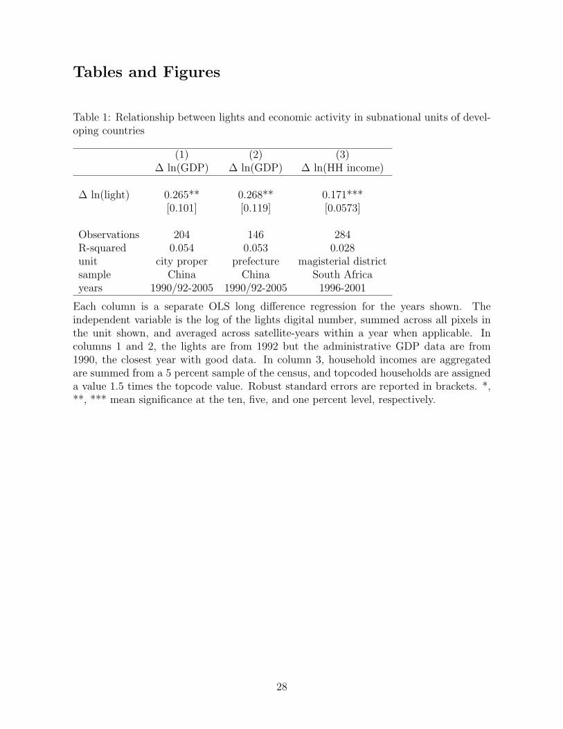
Tables and Figures

Table 1: Relationship between lights and economic activity in subnational units of devel-oping countries

(1) (2) (3)∆ ln(GDP) ∆ ln(GDP) ∆ ln(HH income)

∆ ln(light) 0.265** 0.268** 0.171***[0.101] [0.119] [0.0573]

Observations 204 146 284R-squared 0.054 0.053 0.028unit city proper prefecture magisterial districtsample China China South Africayears 1990/92-2005 1990/92-2005 1996-2001

Each column is a separate OLS long difference regression for the years shown. Theindependent variable is the log of the lights digital number, summed across all pixels inthe unit shown, and averaged across satellite-years within a year when applicable. Incolumns 1 and 2, the lights are from 1992 but the administrative GDP data are from1990, the closest year with good data. In column 3, household incomes are aggregatedare summed from a 5 percent sample of the census, and topcoded households are assigneda value 1.5 times the topcode value. Robust standard errors are reported in brackets. *,**, *** mean significance at the ten, five, and one percent level, respectively.

28

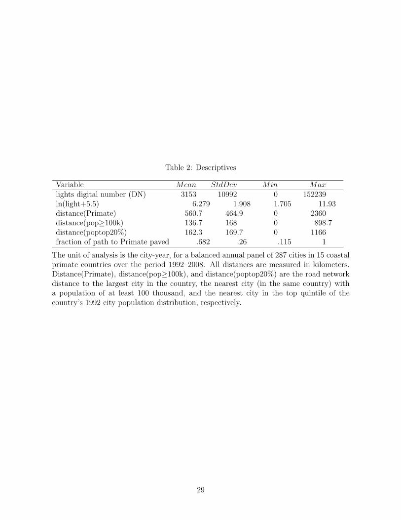
Table 2: Descriptives

Variable Mean StdDev Min Maxlights digital number (DN) 3153 10992 0 152239ln(light+5.5) 6.279 1.908 1.705 11.93distance(Primate) 560.7 464.9 0 2360distance(pop≥100k) 136.7 168 0 898.7distance(poptop20%) 162.3 169.7 0 1166fraction of path to Primate paved .682 .26 .115 1

The unit of analysis is the city-year, for a balanced annual panel of 287 cities in 15 coastalprimate countries over the period 1992–2008. All distances are measured in kilometers.Distance(Primate), distance(pop≥100k), and distance(poptop20%) are the road networkdistance to the largest city in the country, the nearest city (in the same country) witha population of at least 100 thousand, and the nearest city in the top quintile of thecountry’s 1992 city population distribution, respectively.

29

Tab

le3:

Mai

nre

sults

(1)

(2)

(3)

(4)

(5)

(6)

(7)

(8)

ln(l

ight)

ln(l

ight)

ln(l

ight)

ln(l

ight)

ln(l

ight

ln(lig

ht

ln(lig

ht)

ln(l

ight)

+5.

5)+

5.5)

dis

tance

(Pri

mat

e)*P

oil

-0.2

89*

-0.4

04**

*-0

.684

***

-0.6

83**

*-0

.616

***

-0.5

20**

*[0

.154

][0

.151

][0

.240

][0

.223

][0

.215

][0

.169

]dis

t(P

rim

ate)

*ln(P

oil)

-0.3

44**

*[0

.108

]ln

(dis

t(P

rim

ate)

)*ln

(Poil)

-0.0

866*

**[0

.019

4]dis

tance

(Pri

mat

e)-0

.490

0.16

8-0

.539

*[0

.303

][0

.258

][0

.324

]pri

mat

e*ye

ar-0

.039

8***

[0.0

105]

dis

tance

(Pri

mat

e)*y

ear

0.02

27[0

.017

5]pri

mat

e4.

227*

**[0

.238

]

Obse

rvat

ions

4,87

94,

879

4,87

94,

879

4,87

94,

879

4,87

94,

879

model

tobit

tobit

tobit

tobit

OLS

OLS

tobit

tobit

city

FE

sno

no

no

yes

yes

yes

yes

yes

city

tren

ds

non

enon

enon

elinea

rlinea

rsp

lines

linea

rlinea

rle

ftce

nso

red

case

s26

326

326

326

326

326

3

Eac

hco

lum

nis

ase

par

ate

regr

essi

onth

atin

cludes

countr

y*y

earfixed

effec

ts.

The

unit

ofan

alysi

sis

the

city

-yea

r,fo

ra

bal

ance

dan

nual

pan

elof

287

citi

esin

15co

asta

lpri

mat

eco

untr

ies

over

the

per

iod

1992

–200

8.T

he

dep

enden

tva

riab

leis

the

log

ofth

eligh

tsdig

ital

num

ber

,su

mm

edac

ross

allpix

els

inth

eci

ty,an

dav

erag

edac

ross

sate

llite-

year

sw

ithin

aye

arw

hen

applica

ble

.D

ista

nce

(Prim

ate)

isth

ero

adnet

wor

kdis

tance

toth

ela

rges

tci

tyin

the

countr

y,m

easu

red

inth

ousa

nds

ofkilom

eter

s.P

oil

isth

eprice

ofoi

l(s

pec

ifica

lly

the

annual

aver

age

Euro

pe

Bre

nt

Spot

Price

FO

B)

inhundre

ds

ofdol

lars

per

bar

rel.

The

tobit

cuto

ffis

ligh

t=5.

5.R

obust

stan

dar

der

rors

,cl

ust

ered

by

city

,ar

ein

bra

cket

s.*,

**,**

*m

ean

sign

ifica

nce

atth

ete

n,five

,an

don

eper

cent

leve

l,re

spec

tive

ly.

Splines

inco

lum

n6

hav

eon

eknot

per

city

.Sta

ndar

der

rors

hav

enot

bee

nco

rrec

ted

for

the

firs

tst

age

esti

mat

ion.

30

Table 4: Other national trends

(1) (2) (3)ln(lights+5.5) ln(lights+5.5) ln(lights+5.5)

distance(Primate)*Poil -0.959*** -0.963*** -0.503**[0.323] [0.303] [0.228]

distance(Primate)* -0.00385ln(nat. res. income, PPP) [0.0452]

distance(Primate)*ln(GDP, PPP) -0.624[0.605]

Observations 2,819 2,819 4,874

Each column is a separate OLS regression that includes country*year and city fixed ef-fects, and city-specific linear time trends. The unit of analysis is the city-year. Dis-tance(Primate) is the road network distance to the largest city in the country, in thou-sands of kilometers. Poil is the price of oil (specifically the annual average Europe BrentSpot Price FOB) in hundreds of dollars per barrel. Nat. res. income and GDP are naturalresource income and gross domestic product, respectively, in PPP terms. The tobit cutoffis light=5.5. Robust standard errors, clustered by city, are in brackets. *, **, *** meansignificance at the ten, five, and one percent level, respectively.

31

Tab

le5:

Excl

usi

onof

other

chan

nel

sby

whic

hoi

lpri

ces

could

be

affec

ting

ligh

ts

(1)

(2)

(3)

(4)

(5)

(6)

(7)

ln(l

ight)

ln(l

ight)

ln(lig

ht)

ln(l

ight)

ln(l

ight)

ln(l

ight+

5.5)

ln(l

ight+

5.5)

dis

tance

(Pri

mat

e)*P

oil

-0.6

26**

*-0

.606

**-0

.616

***

-0.6

99**

*-0

.448

**[0

.243

][0

.255

][0

.231

][0

.263

][0

.180

]dis

tance

(Pri

mat

e)*P

oil

0.08

10*1

(hydro

clos

est)

[0.2

70]

dis

tance

(Pri

mat

e)*P

die

sel

-0.3

91**

-0.5

05**

*[0

.170

][0

.126

]

Obse

rvat

ions

4,47

14,

029

4,26

73,

128

2,22

62,

226

2,22

6R

-squar

ed0.

580

0.57

9sa

mple

oil>

50km

oil>

100k

mpow

erpla

nt

elec

trifi

eddie

sel

die

sel

die

sel

model

tobit

tobit

tobit

tobit

tobit

OLS

IV:o

il-u

ncl

ust

ered

left

censo

red

case

s24

721

623

012

787

Eac

hco

lum

nis

ase

par

ate

regr

essi

onth

atin

cludes

countr

y*y

ear

and

city

fixed

effec

ts,an

dci

ty-s

pec

ific

linea

rti

me

tren

ds.

The

unit

ofan

alysi

sis

the

city

-yea

r.D

ista

nce

(Pri

mat

e)is

the

road

net

wor

kdis

tance

toth

ela

rges

tci

tyin

the

countr

y,in

thou

sands

ofkilom

eter

s.P

oil

isth

epri

ceof

oil(s

pec

ifica

lly

the

annual

aver

age

Euro

pe

Bre

nt

Spot

Pri

ceFO

B)

inhundre

ds

ofdol

lars

per

bar

rel.

Pdie

selis

the

pri

ceof

die

selin

the

county

’sca

pit

alci

tyin

Nov

ember

ofth

egi

ven

year

,in

dol

lars

per

lite

r.In

colu

mns

1an

d2,

citi

esat

leas

tpar

tial

lyw

ithin

50an

d10

0km

,re

spec

tive

ly,of

anoi

lw

ellar

eex

cluded

.C

olum

n3

incl

udes

only

citi

esin

countr

ies

wit

hbot

hhydro

and

other

pow

erpla

nts

.1(

hydro

clos

est)

isa

dum

my

indic

atin

gth

atth

enea

rest

pow

erpla

nt

toth

eci

tyis

ahydro

pla

nt.

Col

um

n4

incl

udes

only

cities

with

elec

tric

tran

smis

sion

lines

pas

sing

thro

ugh

them

.C

olum

ns

5-7

are

lim

ited

toco

untr

y-y

ears

for

whic

hP

die

sel

isav

aila

ble

.In

colu

mn

7,P

oil

isth

ein

stru

men

tfo

rP

die

sel.

The

tobit

cuto

ffis

ligh

t=5.

5.R

obust

stan

dar

der

rors

,cl

ust

ered

by

city

exce

pt

inco

lum

n7,

are

inbra

cket

s.*,

**,

***

mea

nsi

gnifi

cance

atth

ete

n,five

,an

don

eper

cent

leve

l,re

spec

tive

ly.

32

Tab

le6:

Dis

tance

sto

other

citi

es

(1)

(2)

(3)

(4)

(5)

ln(l

ight)

ln(l

ight)

ln(l

ight)

ln(l

ight)

ln(lig

ht)

dis

tance

(Pri

mat

e)*P

oil

-0.6

83**

*-0

.623

***

-0.5

73**

-0.5

03**

-0.4

43*

[0.2

23]

[0.2

26]

[0.2

25]

[0.2

28]

[0.2

37]

dis

tance

(pop≥

100k

)*P

oil

-0.5

35[0

.501

]dis

tance

(pop≥

100k

)*P

oil*1

(nea

rest

pop≥

100k

isn’t

pri

mat

e)-0

.888

[0.7

36]

dis

tance

(pop

top20

%)*

Poil

-1.2

05**

[0.4

85]

dis

tance

(pop

top20

%)*

Poil*1

(nea

rest

pop

top20

%is

n’t

pri

mat

e)-1

.240

**[0

.610

]

Obse

rvat

ions

4,87

94,

879

4,87

94,

879

4,87

9le

ftce

nso

red

case

s26

326

326

326

326

3

Eac

hco

lum

nis

ase

par

ate

tobit

regr

essi

onth

atin

cludes

countr

y*y

ear

and

city

fixed

effec

ts,an

dci

ty-s

pec

ific

linea

rtim

etr

ends.

The

unit

ofan

alysi

sis

the

city

-yea

r,fo

ra

bal

ance

dan

nual

pan

elof

287

citi

esin

15co

asta

lpri

mat

eco

untr

ies

over

the

per

iod

1992

–200

8.T

he

dep

enden

tva

riab

leis

the

log

ofth

eligh

tsdig

ital

num

ber

,su

mm

edac

ross

allpix

els

inth

eci

ty,an

dav

erag

edac

ross

sate

llit

e-ye

ars

wit

hin

aye

arw

hen

applica

ble

.D

ista

nce

(Pri

mat

e),dis

tance

(pop≥

100k

),an

ddis

tance

(pop

top20

%)

are

the

road

net

wor

kdis

tance

toth

ela

rges

tci

tyin

the

countr

y,th

enea

rest

city

(in

the

sam

eco

untr

y)

wit

ha

pop

ula

tion

ofat

leas

t10

0th

ousa

nd,an

dth

enea

rest

city

inth

eto

pquin

tile

ofth

eco

untr

y’s

1992

city

pop

ula

tion

,re

spec

tive

ly.

Dis

tance

sar

em

easu

red

inth

ousa

nds

ofkilom

eter

s.P

oil

isth

epri

ceof

oil(s

pec

ifica

lly

the

annual

aver

age

Euro

pe

Bre

nt

Spot

Pri

ceFO

B)

inhundre

ds

ofdol

lars

per

bar

rel.

The

dum

my

variab

les

inte

ract

edw

ith

thes

edis

tance

sin

colu

mns

(3)

and

(5)

are

one

ifth

enea

rest

larg

eci

ty(o

f10

0kin

colu

mn

3,or

inth

eto

pquin

tile

inco

lum

n5)

isnot

the

pri

mat

e.T

he

tobit

cuto

ffis

ligh

t=5.

5.R

obust

stan

dar

der

rors

,cl

ust

ered

by

city

,ar

ein

bra

cket

s.*,

**,**

*m

ean

sign

ifica

nce

atth

ete

n,five

,an

don

eper

cent

leve

l,re

spec

tive

ly.

33

Tab

le7:

Pav

ing

and

city

size

(1)

(2)

(3)

(4)

(5)

ln(l

ight)

ln(l

ight)

ln(p

opula

tion

)ln

(lig

ht+

5.5)

frac

tion

man

ufa

cturing

1(pav

ing

>m

edia

n)

0.28

0***

0.58

4**

0.01

51**

*[0

.106

][0

.275

][0

.005

21]

dis

t(prim

ate)

*Poil

-0.6

53**

*-0

.640

***

[0.2

13]

[0.2

07]

dis

tance

(Pri

mat

e)-0

.079

10.

0633

-0.0

196*

*[0

.135

][0

.366

][0

.009

43]

Obse

rvat

ions

4,87

94,

879

272

272

293

R-s

quar

ed0.

258

0.50

6sa

mple

all

all

non

-pri

mat

eci

ties

non

-pri

mat

eci

ties

IPU

MS

model

tobit

tobit

OLS

tobit

OLS

unit

city

city

city

city

dis

tric

tdir

tfa

ctor

1.5

2le

ftce

nso

red

case

s26

326

352

Eac

hco

lum

nis

ase

par

ate

regr

essi

on,w

ith

countr

yfixed

effec

ts.

Col

um

ns

1an

d2

are

anal

ogou

sto

the

bas

elin

esp

ecifi

cati

onw

ith

route

dis

tance

sca

lcula

ted

diff

eren

tly.

Dirt

fact

oris

the

rati

oof

the

tim

ere

quir

edto

trav

erse

agi

ven

lengt

hof

dir

tro

adan

dth

eti

me

requir

edto

trav

erse

the

sam

ele

ngt

hof

pav

edro

ad,

use

din

calc

ula

ting

shor

test

route

s.In

colu

mns

3-5,

the

indep

enden

tva

riab

leof

inte

rest

isa

dum

my

indic

atin

gth

atth

eunit

’spat

hto

its

countr

y’s

pri

mat

eci

tyis

mor

epav

edth

anth

eav

erag

ew

ithin

that

countr

y.In

colu

mns

3an

d4,

the

sam

ple

is27

2non

-prim

ate

cities

in15

coas

talpri

mat

eco

untr

ies

in19

92,

the

init

ialye

ar.

Inco

lum

n3,

the

dep

enden

tva

riab

leis

the

log

ofpop

ula

tion

,w

hile

inco

lum

n2

itis

the

log

ofth

eligh

tsdig

ital

num

ber

,su

mm

edac

ross

allpix

els

inth

eci

ty,an

dav

erag

edac

ross

sate

llit

e-ye

ars

wit

hin

aye

arw

hen

applica

ble

.In

colu

mn

3,th

esa

mple

isce

nsu

sad

min

istr

ativ

eunit

sin

Ghan

a(2

000)

,G

uin

ea(1

983)

,Sen

egal

(198

8),an

dTan

zania

(200

2),an

dth

edep

enden

tva

riab

leis

frac

tion

ofth

eem

plo

yed

pop

ula

tion

over

age

10w

orkin

gin

man

ufa

cturi

ng.

Dis

tance

(Pri

mat

e)is

the

road

net

wor

kdis

tance

toth

ela

rges

tci

tyin

the

countr

y,m

easu

red

inth

ousa

nds

ofkilom

eter

s.T

he

tobit

cuto

ffis

ligh

t=5.

5.R

obust

stan

dar

der

rors

,cl

ust

ered

by

city

inco

lum

ns

1an

d2,

are

inbra

cket

s.*,

**,**

*m

ean

sign

ifica

nce

atth

ete

n,five

,an

don

eper

cent

leve

l,re

spec

tive

ly.

34

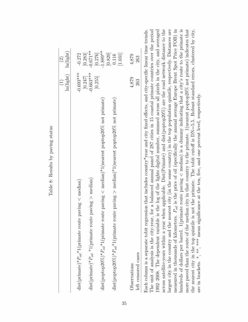
Tab

le8:

Res

ult

sby

pav

ing

stat

us

(1)

(2)

ln(l

ight)

ln(lig

ht)

dis

t(prim

ate)

*Poil*1

(pri

mat

ero

ute

pav

ing

<m

edia

n)

-0.6

93**

*-0

.272

[0.2

47]

[0.2

83]

dis

t(prim

ate)

*Poil

*1(p

rim

ate

route

pav

ing

>m

edia

n)

-0.6

63**

*-0

.671

**[0

.255

][0

.276

]dis

t(pop

top20

%)*

Poil*1

(pri

mat

ero

ute

pav

ing

<m

edia

n)*

1(nea

rest

pop

top20

%not

prim

ate)

-1.8

89**

[0.8

20]

dis

t(pop

top20

%)*

Poil*1

(pri

mat

ero

ute

pav

ing

>m

edia

n)*

1(nea

rest

pop

top20

%not

prim

ate)

0.11

6[1

.031

]

Obse

rvat

ions

4,87

94,

879

left

censo

red

case

s26

326

3

Eac

hco

lum

nis

ase

par

ate

tobit

regr

essi

onth

atin

cludes

countr

y*y

ear

and

city

fixed

effec

ts,an

dci

ty-s

pec

ific

linea

rtim

etr

ends.

The

unit

ofan

alysi

sis

the

city

-yea

r,fo

ra

bal

ance

dan

nual

pan

elof

287

citi

esin

15co

asta

lpri

mat

eco

untr

ies

over

the

per

iod

1992

–200

8.T

he

dep

enden

tva

riab

leis

the

log

ofth

eligh

tsdig

ital

num

ber

,su

mm

edac

ross

allpix

els

inth

eci

ty,an

dav

erag

edac

ross

sate

llit

e-ye

ars

wit

hin

aye

arw

hen

applica

ble

.D

ist(

Pri

mat

e)an

ddis

t(pop

top20

%)

are

the

road

net

wor

kdis

tance

toth

ela

rges

tci

tyin

the

countr

yan

dth

enea

rest

city

(in

the

sam

eco

untr

y)

inth

eto

ppop

ula

tion

quin

tile

,re

spec

tive

ly.

Dis

tance

sar

em

easu

red

inth

ousa

nds

ofkilom

eter

s.P

oil

isth

epri

ceof

oil(s

pec

ifica

lly

the

annual

aver

age

Euro

pe

Bre

nt

Spot

Pri

ceFO

B)

inhundre

ds

ofdol

lars

per

bar

rel.

1(pri

mat

ero

ute

pav

ing

<m

edia

n)

isa

dum

my

indic

atin

gth

ata

city

’sro

ute

toth

epri

mat

eis

mor

epav

edth

anth

ero

ute

ofth

em

edia

nci

tyin

that

countr

yto

the

pri

mat

e.1(

nea

rest

pop

top20

%not

pri

mat

e)in

dic

ates

that

the

nea

rest

city

inth

eto

pquin

tile

isnot

the

pri

mat

e.T

he

tobit

cuto

ffis

DN

=5.

5.R

obust

stan

dar

der

rors

,cl

ust

ered

by

city

,ar

ein

bra

cket

s.*,

**,**

*m

ean

sign

ifica

nce

atth

ete

n,five

,an

don

eper

cent

leve

l,re

spec

tive

ly.

35

!(

!(

!(

!(

!(

!(

!(

!(

!(!(

!(

!(!(

!(

!(

!(

!(

!(

!(

!(

!(

!(

!(

!(

!(

!(

!(

!(

!(

!(

!(

!(

!(

!(!(

!(

!(Pr

imate

city

coas

tal pr

imate

landlo

cked

multip

olar

no da

ta0

1,000

2,000

500

km

Mauri

tania

Sene

gal

Guine

a

Sierra

Leon

eLib

eria Co

te d'I

voire

Ghan

a

Togo

Benin

Came

roon

Gabo

n

Moza

mbiqu

eTanz

ania

Ango

la

Nigeri

a

Fig

ure

1:A

fric

anco

untr

iescl

assi

fied

by

thei

rco

asta

lacc

ess,

the

coas

tala

cces

sof

thei

rpri

mat

eci

ty,an

dav

aila

bility

ofco

mpar

able

road

san

dligh

tsdat

a

36

Satel

lite F-

16, 2

008

High :

63

Low

: 0Na

tiona

l bord

ers

020

040

010

0km

Fig

ure

2:Lig

hts

dig

ital

num

ber

inTan

zania

from

sate

llit

eF-1

6,20

08

37

Satel

lite F-

16, 2

008

High :

63

Low

: 0Na

tiona

l bord

ers

010

205

km

Fig

ure

3:Lig

hts

dig

ital

num

ber

inan

dar

ound

Dar

esSal

aam

,Tan

zania

from

sate

llit

eF-1

6,20

08

38

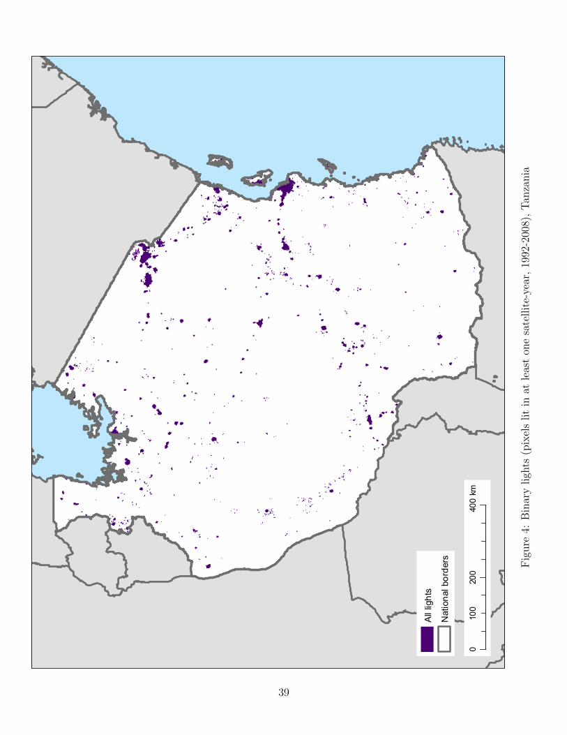
All lig

htsNa

tiona

l bord

ers

020

040

010

0km

Fig

ure

4:B

inar

yligh

ts(p

ixel

slit

inat

leas

ton

esa

tellit

e-ye

ar,19

92-2

008)

,Tan

zania

39

!

!

!

!

!

!

!

!

!

!

!

!!

!

!

!

!

!

!

!

!

!!

!

!

!

!

!

!

!

!!

!

!

!!

!

!

!

!

!

!

!

!

!

!

!

!

!

!!

!

!

!

!

!!

!

!

!

!

!

!

!!

!

!

!

!

!

!

!

!

!

!

!

!

!

!

!

!

!

!

!

!

!

!

!

!

!

!

!

!

!

!

!

!

!

!

!!

!

!

!

!

!

Wete

Same

Magu

Vwaw

a

Uyov

u

Tang

a

Nzeg

a

Nkom

eNg

udu

Mosh

i

Mbulu

Mbey

a

Lindi

Kyela

Itigi

Ilula

Gairo

Chato

Bund

a

Uram

bo

Tuku

yu

Tarim

e

Tabo

ra

Song

ea

Sirari

Njomb

e

Nans

io

Mwan

za

Mwan

ga

Muso

ma

Muhe

za

Mugu

mu

Mtwa

ra

Mpan

da

Mlim

ba

Miku

mi

Mbing

aMa

sasi

Liwale

Kond

oa

Kises

a

Kilos

a

Kigom

a

Kidod

iKid

atuKib

iti

Kator

o

Kasu

lu

Kaha

ma

Iringa

Igung

aHe

daru

Dodo

ma

Buko

ba

Baba

ti

Arus

ha Tund

uru

Tomo

ndo

Singid

a

Nyak

ato

Nguru

ka

Mpwa

pwa

Many

oni

Mafin

ga

Korog

we

Kiomb

oi

Kimam

ba

Kibon

doIsa

gehe

Ifaka

ra

Baria

di

Zanz

ibar

Morog

oroMl

andiz

i

Masu

mbwe

Mapo

seni

Mago

goni

Ikwirir

i

Chali

nze

Ushir

ombo

Usa R

iver

Shiny

anga

Nama

nyere

Maka

mbak

o

Tand

ahim

ba

Sumb

awan

ga

Nach

ingwe

a

Chak

e Cha

ke

Kiemb

esam

aki

Dar e

s Sala

am

Newa

la (Lu

ching

u)

Misu

ngwi

(Mab

uki)

Hand

eni (C

hanik

a)

Masw

a (Ny

aliku

ngu)

Kong

wa (-K

ibaigw

a)

Hai (H

ai Dis

trict)

Merer

ani (S

iman

jiro D

istric

t)

!Cit

y poin

tsAll

lights

Natio

nal b

orders

020

040

010

0km

Fig

ure

5:B

inar

yligh

tsan

dci

ties

wit

hknow

npop

ula

tion

s,Tan

zania

40

Popu

lated

Ligh

tsNa

tiona

l bord

ers

020

040

010

0km

Fig

ure

6:B

inar

yligh

ts,re

stri

cted

toci

ties

wit

hknow

npop

ula

tion

s,Tan

zania

41

.4.6.811.2diesel price, dollars/liter

20406080100oil price, dollars/barrel

1992

1994

1996

1998

2000

2002

2004

2006

2008

year

oil p

rice,

dol

lars

/bar

rel

dies

el p

rice,

dol

lars

/lite

r

Fig

ure

7:O

ilan

ddie

sel

pri

ces

(ave

rage

dac

ross

the

12co

untr

ies

inth

esa

mple

wit

hdat

afo

ral

l7

year

ssh

own),

1992

–200

8.D

iese

lprice

sw

ere

surv

eyed

inN

ovem

ber

,w

hile

oilpri

ces

are

aver

aged

acro

ssth

ew

hol

eye

ar.

42

Popu

lated

Ligh

tsUn

pave

d roa

dsPa

ved r

oads

Natio

nal b

orders

020

040

010

0km

Fig

ure

8:R

oads

inTan

zania

43

Popu

lated

Ligh

tsSe

lected

road

sUn

pave

d roa

dsPa

ved r

oads

Natio

nal b

orders

020

040

010

0km

Fig

ure

9:Shor

test

road

route

sfr

omci

ties

wit

hknow

npop

ula

tion

sto

Dar

esSal

aam

,Tan

zania

44

Fig

ure

10:

Dia

gram

ofth

epav

ing

resu

lts.

Thre

eci

ties

,A

,B

,an

dC

,id

entica

lex

cept

for

thei

rlo

cation

s,ar

eco

nnec

ted

toa

pri

mat

eci

tyP

and

ase

condar

y(i

.e.

top

quin

tile

)ci

tyS,w

ith

the

dis

tance

rela

tion

ship

sd

SA

=d

SB

<d

SC

<d

PC

=d

PB

<d

PA.

When

oilpri

ceri

se,if

road

sPA

,P

Ban

dP

Car

epav

ed(l

eft

figu

re),

Aw

illgr

owsl

ower

than

B,w

hic

hw

illgr

owab

out

asfa

stas

C.If

thes

eth

ree

road

sar

eunpav

ed(r

ight

figu

re),

Aan

dB

willgr

owat

the

sam

era

te,fa

ster

than

C.

45

A Data and spatial methods

A.1 City points

City locations (latitude and longitude) and census populations were collected from the

City Population website and spot-checked with official sources where available.49 Using

city-specific growth rates based on multiple censuses where available, or national urban

growth rates from United Nations (2008) otherwise, I generated a population for all years

for each city.

For 14 of the 15 countries in the ultimate sample, City Population claims to list all

cities above a given (country-specific) population, typically 5,000, 10,000, or 20,000.50

However, it does not explicitly cite the year for which this claim is made. Of the 738

cities with location and population information in these 15 countries, 9 city points fall

below this cutoff for all years 1990 to 2008. These are included in the sample until explicit

population cuts are made.

A.2 Lights

The lights data are described in Henderson, Storeygard and Weil (2012). For the present

study the 30 satellite-years of lights data were first combined into one binary grid encoding

whether a pixel was lit in at least one satellite-year. The resulting contiguous ever-lit

areas were converted into polygons, and split by national borders. Only lights within 3

kilometers of one of the city points described above with a known census population were

kept in the sample. The 3-km buffer is used because of georeferencing error in both the

points and the lights (Balk et al., 2004; Elvidge et al., 2004). While some of the other

lights are likely to be small settlements, some are noise from the sensor or from fires lasting

for too long to be excluded by the data cleaning algorithm, mines or other facilities. In

general, they are smaller and weaker lights as well.

The resulting sample is 485 lights in 15 countries. Populations for each point were

summed across all points assigned to each light. In 49 lights, more than one city was

present; in 26 of these, exactly two were present. In 13 cases, a point fell within 3

km of multiple lights. In such cases, the point’s population was only retained by the

light to which it was closest. The light with the largest 1992 population within each

country was designated the primate. In most countries, this corresponded to the historical

49http://www.citypopulation.de/. In 9 cases where coordinates or population were unavailable fromCity Population, coordinates from Google Earth or World Gazetteer (http://www.world-gazetteer.com)were used.

50For Angola, there is no explicit cutoff.

46

political capital. The only exception is Douala, Cameroon, which is larger than Yaounde.

The historical political capitals that are not current formal political capitals are Dar es

Salaam, Tanzania, which was replaced by Dodoma, Abidjan, Cote d’Ivoire, replaced by

Yamoussoukro, and Lagos, Nigeria, replaced by Abuja.

A.3 Roads

The African Infrastructure Country Diagnostic database contains comparable roads data

for all countries of the African mainland with no Mediterranean coastline, plus Mada-

gascar, except for Djibouti, Equatorial Guinea, Guinea-Bissau, and Somalia.51 Two

datasets were produced for Sudan: one for the north and one for the south. The

datasets generally have comparable metadata on road surface, quality, and hierarchy

(primary/secondary/tertiary), as well as estimates of traffic. Still before they could be

used for the current analysis, several changes had to be made. All steps below were carried

out using ArcGIS 9.3 software, except for some tabular cleaning done in Excel and Stata.

Nearly all steps in ArcGIS, and all steps in Stata, were automated in Python, Arc Macro

Language (AML), or Stata scripts.

The roads data were cleaned tabularly, to ensure that the relevant fields were coded

consistently, and projected to a sinusoidal projection, which is more conducive to distance

calculations than their native plate carree (latitude and longitude).52 Next, roads from

all countries were combined into one large dataset, and a topology was built with the rule

“no dangles”. This means that every dead end was flagged. In most cases, dead ends are

legitimate features of the road network. In other cases, however, they are artifacts of a

data generation process in which some segments that are connected in the real world are

not connected in the dataset. This is critical in the network analysis to follow.

Problematic dangles were fixed in several ways. First, using the topology “Extend”

tool, dangles were extended up to 100 meters if that would cause them to no longer be

dangles. In theory, the topology “Trim” tool could be used for the opposite task to dangles

less than 100 meters long. However, a bug in ArcGIS made this infeasible. But extra

dangles only affect final results to the extent that they cause additional “spiders” to be

created (see below).

The Extend operation does not close all gaps of less than 100 meters. To see this,

imagine the forward slash and backslash characters typed with a space between them:

/ \. Extending either character individually, even by doubling its length, would not make

the two touch, because they are pointed in the wrong direction. To deal with cases like

51http://www.infrastructureafrica.org/52The projection’s central meridian is 15 degrees east longitude.

47

these, “bridges” were created as follows. All dangles were paired with the closest other

dangle if it was within 100 meters using the Spatial Join tool, and connecting lines were

created between these pairs of dangles. These bridges were added to the rest of the roads.

The AICD roads database was gathered with explicit reference to inter-city roads.

Unfortunately, this means that in many cases, information on roads within cities was not

collected, greatly reducing the connectivity of the dataset in many countries. “Spiders”

were created to model missing city roads. For every dangle falling within a city, a (paved)

road was created between the city centroid and the dangle. The implicit assumption is that

radial road travel within cities is comparatively easy. The resulting spiders were added

to the roads, and all spiderlegs and any roads that intersected them were “planarized”.

Before planarizing, the topology of the network was such that a spiderleg could cross a

road without being connected to it. Planarizing ended this.

Manual edits were necessary for several reasons. Recall that Extend did not close

holes if a dangle was not pointed at another road, and that bridges were only created

between two nearby dangles, not a dangle and a non-dangle. So extra segments of less

than 10 meters each were created in 6 other places to fix dangles affecting routes to 16

cities. Recall also that spiders were created between a centroid and any dangles within a

city. So once a spider is created, the spiderleg is the network location of the centroid, so

if it connects to a dead end, other nearby roads cannot be reached even if they are very

close. In these cases, deleting one or more spiderlegs fixed the problem. Five spiderlegs

affecting 4 cities were deleted.

A.4 Route calculation

To prepare for building the network, the roads were intersected with all land borders,

so that the resulting border posts could be used as barriers—non-traversable points on

the network. Coastlines were not treated as borders in this operation, because the only

reason a road would cross a coastline is because of misalignment—the resulting route is

most likely legitimate.

A network dataset was built using the roads dataset. The “Closest Facility” solver

was used with the following settings. All light centroids were used as the “Incidents”,

centroids of primate cities were used as “Facilities”, and the intersections of the roads

and the land borders were used as “Barriers”. Each city was assigned a network location

on the closest road within 5 kilometers of its centroid.

Unfortunately, because of a quirk in the program, the total calculated length is a true

geodesic distance, while distances by paving status are projected distances. However, this

48

never causes a discrepancy of more than a few percent, and because the same projection

is used for the whole continent, these errors are highly correlated within countries.

Of 485 populated lights, 464 (96 percent) received plausible routes. Of the remaining

21, 6 were in exclaves or islands, and 2 had centroids more than 5 km from the nearest

domestic road. Three received no routes because they were on road segments disconnected

from the primate by a gap of at least 100 meters. The remaining ten received implausible

routes (because of suspicious gaps of longer than 100 meters in the road network) and

were removed. To the extent that these cities are in fact less connected than others, or

that government officials have not mapped their roads correctly or at all, they are more

likely to be excluded from traditional data sources like censuses and surveys as well.

A.5 Pixel-level data-generating process

The pixel-level data-generating process can be modeled as follows:

yjist =

0 if y∗jist < 2.5 or

∑k∈i 1{y∗kist >= 2.5} < 4

63 if y∗jist > 62.5

int(y∗jist + 0.5) otherwise

(14)

where j indexes pixels, which nest in cities, s indexes satellite-years within a year, yjist

is measured pixel-level light, and y∗jist is true (latent) pixel-level light. Two nonlinearities

appear here, in addition to rounding to the nearest integer. Processing by NOAA converts

to zero nearly all (1) individual pixel values of 1 or 2 and (2) clusters of less than 4 nonzero

pixels. In both cases, NOAA’s algorithm interprets these patterns as random noise.

The relationship of interest is at the city level, as are all of the regressors, but the lights

data are generated nonlinearly at the pixel level. Rather than estimate Equation (14) via

maximum likelihood with approximately 5.6 million pixel-satellite-years, I instead simply

sum lights across pixels and satellites within a city:

yit = (1/St)St∑

s=1

∑j∈i

yjist (15)

where St is the number of active satellites (always 1 or 2), and run a tobit regression with

a cutoff value of 5.5. The theoretical minimum non-zero city-year has a DN value of 6: in

one satellite-year it is unlit, while in the other satellite-year, it consists of 4 pixels, each

with a DN of 3. In practice, this is also the minimum non-zero city-year DN value in the

estimation sample.

49

0.51diesel price, dollars/liter

1992

1994

1996

1998

2000

2002

2004

2006

2008

year

Nig

eria

Gab

onA

ngol

a

Fig

ure

A.1

:D

iese

lpri

ces

for

the

oilpro

duci

ng

countr

ies,

1993

–200

8

50