farm-level mathematical programming tools for agricultural

.A®L.

~ 111111 UNIVERSITEIT

GENT FACULTEIT BlO-INGENIEURSWETENSCHAPPEN

® . .

“All models are wrong, but some are useful.” (Howitt, 2005)

I

Promotor: Prof. G. Van Huylenbroeck Department of Agricultural Economics Dean: Prof. H. Van Langenhove Rector: Prof. P. Van Cauwenberge

II

Jeroen Buysse

Farm-level mathematical programming tools for agricultural policy support

Thesis submitted in fulfillment of the requirements for the degree of Doctor (PhD) in Applied Biological Sciences

III

Dutch translation of the title: Bedrijfsspecifieke mathematische programmeringsmethoden voor landbouwbeleidsondersteuning ISBN-number: 90-5989-133-3 The author and the promotor give the authorisation to consult and to copy parts of this work for personal use only. Every other use is subject to the copyright laws. Permission to reproduce any material contained in this work should be obtained from the author

IV

Voorwoord / Preface

Sinds mijn eerste stapjes programmeerwerk met een rekenmachine ben ik geïnspireerd door

het concept dat het samenbrengen van een aantal eenvoudige rekenregels kunnen leiden tot

verbazend vernuftige systemen. Het is voor mij ook een uitdaging geworden om complexe

systemen te proberen ontleden en op te delen in kleine en eenvoudige stapjes. Deze

bewondering voor de eenvoud heeft me gemotiveerd tot het maken van dit doctoraat.

Ik ben Prof. Guido Van Huylenbroeck dan ook zeer dankbaar omdat hij me de kans heeft

gegeven om te werken aan een bio-economisch simulatiemodel van een melkveebedrijf en

later aan het SEPALE project. Er bestaat geen twijfel over het feit dat zonder deze kansen,

aanmoedigingen en steun van Prof. Guido Van Huylenbroeck dit doctoraat er niet zou

geweest zijn.

Bij de uitwerking van het onderzoek heb ik gelukkig ook kunnen rekenen op de hulp van de

andere mensen met wie ik heb samengewerkt: de collega’s in het SEPALE project, collega’s

van de vakgroep landbouweconomie en van Stedula.

Voor de gegevensverzameling kon ik rekenen op de goede samenwerking met Bruno

Fernagut en Ludwig Lauwers en Prof. Bruno Henry de Frahan hebben een belangrijke

bijdrage geleverd aan de teksten die in dit doctoraat gebruikt zijn.

De collega’s van de vakgroep Landbouweconomie hebben de aangename sfeer bepaald

waarin ik de afgelopen vijf jaar gewerkt heb. Zij hebben regelmatig de rol van klankbord op

zich genomen, de kaft ontworpen (Ann Verspecht) en tussendoor ook voor de nodige

(sportieve) ontspanning gezorgd.

Verder zou ik ook zeker de leden van de examencommissie willen bedanken voor de

evaluaties en de suggesties tot verbetering van dit proefschrift.

Ouders, familie en vrienden zou ik willen bedanken voor de kansen, appreciatie en

vertrouwen en omdat zij me kennis en betrokkenheid met de landbouwpraktijk hebben

gegeven die zeer nuttig zijn geweest bij de theoretische uitwerking van dit doctoraat.

Tot slot zou ik nog mijn vrouw Sara willen bedanken. Zij heeft me tijdens mijn volledige

universitaire studies en doctoraatsonderzoek met veel liefde ondersteund.

V

Table of contents

General Introduction .................................................................................................................. 1 Why farm-level models? ........................................................................................................ 2 Arguments for using programming models ........................................................................... 4 Objective: description of 3 types of MP................................................................................. 8

Chapter 1 Overview of the three types of programming models.......................................... 11 1.1 Introduction .............................................................................................................. 12 1.2 Normative mathematical programming (NMP) ....................................................... 13

1.2.1 Arguments for using NMP in agricultural policy analysis............................... 13 1.2.2 Normative model to predict participation to meadow bird management......... 16

1.3 Positive mathematical programming (PMP) ............................................................ 19 1.3.1 Calibration of farm-level MP models............................................................... 19 1.3.2 PMP model to predict participation to meadow bird management .................. 23

1.4 Econometric mathematical programming (EMP) .................................................... 28 1.5 Conclusions .............................................................................................................. 30

Chapter 2 An application of farm level NMP: Simulating the influence of management decisions on the nutrient balance of dairy farms...................................................................... 31

2.1 Introduction .............................................................................................................. 32 2.2 The simulation model............................................................................................... 33 2.3 General model .......................................................................................................... 34

2.3.1 Animal production............................................................................................ 35 2.3.2 Grazing strategy ............................................................................................... 36 2.3.3 Nutrient cycling aspects ................................................................................... 38

2.4 Validation ................................................................................................................. 38 2.5 Simulation results..................................................................................................... 40

2.5.1 Influence of the summer ration ........................................................................ 40 2.5.2 Influence of the grassland - maize ratio ........................................................... 42 2.5.3 Summer milk, winter milk and zero grazing.................................................... 44

2.6 Sensitivity analysis................................................................................................... 45 2.7 Discussion ................................................................................................................ 48 2.8 Conclusions .............................................................................................................. 50

2.8.1 Conclusions with respect to the application..................................................... 50 2.8.2 Modelling lessons............................................................................................. 50 2.8.3 Other experiences from the dairy farm model ................................................. 52

Chapter 3 Positive Mathematical Programming: introduction to the farm-level calibrated model SEPALE ........................................................................................................................ 53

3.1 Introduction .............................................................................................................. 54 3.2 The original PMP Approach .................................................................................... 56 3.3 Discussion of the original PMP Approach............................................................... 60 3.4 Further PMP developments...................................................................................... 62 3.5 SEPALE: System for evaluation of agro- and agro-environmental policies. .......... 63

3.5.1 Description of the basic farm model ................................................................ 64 3.5.2 Simulation of the Mid-term Review of Agenda 2000...................................... 66 3.5.3 Impact analysis ................................................................................................. 72

3.6 Conclusions .............................................................................................................. 76 3.6.1 Conclusions with respect to the applications ................................................... 76 3.6.2 Modelling lessons............................................................................................. 77

VI

Chapter 4 PMP extension of SEPALE: modelling the impact of policy reforms on Belgian sugar beet suppliers..................................................................................................... 83

4.1 Introduction .............................................................................................................. 86 4.1.1 The EU sugar CMO.......................................................................................... 86 4.1.2 EU sugar CMO reform..................................................................................... 87 4.1.3 Other EU sugar CMO reform analysises.......................................................... 88

4.2 C sugar beet supply .................................................................................................. 90 4.2.1 Yield variation function ................................................................................... 92 4.2.2 Precautionary supply function.......................................................................... 98

4.3 Quota rent approximation and sugar beet model calibration ................................. 101 4.4 Quota transfer ......................................................................................................... 103 4.5 Calibration and simulation results.......................................................................... 104

4.5.1 Supply effects of price and quota reductions ................................................. 107 4.5.2 Supply effects of a combined price reduction and quota reduction or increase 109 4.5.3 Supply effects of compensation mechanisms................................................. 110 4.5.4 Income effects of price and quota reductions................................................. 111 4.5.5 Supply effects on other crops ......................................................................... 113 4.5.6 Supply and income effects according to farm size and region....................... 114 4.5.7 Sensitivity analysis on the quota rent approximation..................................... 114

4.6 Conclusions ............................................................................................................ 116 4.6.1 Conclusions with respect to the application................................................... 116 4.6.2 Modelling lessons........................................................................................... 117

Chapter 5 EMP extension of SEPALE ............................................................................... 119 5.1 Introduction ............................................................................................................ 120 5.2 Application: estimation of the C sugar beet precaution supply function ............... 121 5.3 Calibration and simulation results.......................................................................... 127

5.3.1 Identification of farm groups.......................................................................... 128 5.3.2 Supply effects of price and quota reductions ................................................. 131 5.3.3 Supply effects of a combined price reduction and quota reduction or increase... ........................................................................................................................ 135 5.3.4 Supply effects of compensation mechanisms................................................. 140 5.3.5 Income effects of price and quota reductions................................................. 142 5.3.6 Supply effects on other crops ......................................................................... 147

5.4 Conclusions ............................................................................................................ 148 5.4.1 Conclusions with respect to the application................................................... 148 5.4.2 Modelling lessons........................................................................................... 148

General discussion and conclusion ........................................................................................ 151 Definition and classification of the 3 model types ............................................................. 151 Summarising overview of the applications of the three model types ................................ 153 Model type selection .......................................................................................................... 155 Some concluding remarks and recommendations for further research .............................. 156

References .............................................................................................................................. 159

Summary ................................................................................................................................ 169

Samenvatting.......................................................................................................................... 172

Scientific curriculum vitae ..................................................................................................... 175

VII

List of tables

Table 1. Characteristics of the hypothetical farm............................................................... 17

Table 2. Empirical data of two hypothetical farms under the assumption of a 300 euro/ha

compensation for extensive grassland.............................................................................. 23

Table 3. Input data for cows............................................................................................... 35

Table 4. Farm characteristics included in the model.......................................................... 39

Table 5. Comparison of observed and simulated farm data. .............................................. 39

Table 6. Comparison of sample and population for the 2002 calibration year ................ 104

Table 7. Farm characteristics of the sample for the 2002 calibration year ...................... 105

Table 8. Calibrated cost function parameters and supply elasticities from the FADN crop .

farm sample ........................................................................................................ 105

Table 9. Changes in the aggregate crop supply as a result of the June 2003 CAP reform.....

............................................................................................................................ 106

Table 10. Changes in the aggregate sugar beet supply and quota rent from a reduction in A

sugar beet price................................................................................................... 108

Table 11. Changes in the aggregate sugar beet supply and quota rent from a reduction in ....

sugar beet quota.................................................................................................. 109

Table 12. Changes in aggregate sugar beet supply and quota rent from changes in sugar .....

beet quota and price............................................................................................ 110

Table 13. Effects of a price reduction compensation of 64,2% on the supply of selected

crops of sugar beet farms within the Belgian FADN for a 39,5% reduction in A

sugar beet price................................................................................................... 114

Table 14. Effects of the accepted sugar CMO reform according to size classes and regions ..

............................................................................................................................ 114

Table 15. Changes in the aggregate sugar beet supply and quota rent from A sugar beet ......

price and quota reductions with different initial approximated quota rents....... 115

Table 16. Key results of the estimation of the sugar module ............................................. 126

VIII

Table 17. GME parameter estimates of the sugar beet programme from a sensitivity ...........

analysis on the support intervals ........................................................................ 127

Table 18. Changes in the aggregate crop supply as a result of the June 2003 CAP reform.....

............................................................................................................................ 127

Table 19. Distribution of the farms over the different regions........................................... 129

Table 20. Average acreage of different crops for the 4 farm groups (in ha)...................... 130

Table 21. Average precaution parameters for the 4 farm groups....................................... 130


crops of sugar beet farms within the Belgian FADN for a 39,5% reduction in A

sugar beet price................................................................................................... 147

IX

List of figures

Figure 1. Outline of the dissertation .................................................................................... 10

Figure 2. Graphical illustration of a simplified NMP farm model with two activities (X1

and X2) and a profit maximising objective function............................................ 15

Figure 3. The impact of the compensation level for extensively managed grassland on the

production of the different activities on the dairy farm ....................................... 18

Figure 4. Graphical illustration of a PMP simplified farm model with two activities (X1

and X2) and a profit maximising function ........................................................... 21


production of the extensively managed grass on the dairy farm.......................... 26

Figure 6. Relationship between different modules in the model ......................................... 34

Figure 7. Influence of the summer ration on the N – surplus of the ■ summer milk farm

system and the □ winter milk farm system .......................................................... 41

Figure 8. Growth curve of grass under the mowing ▬ and grazing ▬ regime .................. 42

Figure 9. Influence of the grassland – maize ratio on the N – surplus (kg / ha) for the

summer milk farm system (■) and the winter milk farm system (□) ................... 43

Figure 10. Influence of the grassland – maize ratio on the N – surplus (■) and P - surplus

(□) in case of zero grazing................................................................................ 44

Figure 11. Annual variation of N – input for the whole herd on the summer milk, zero

grazing and the winter milk farm systems. ...................................................... 45

Figure 12. N – surplus with three N – fertilization levels for the summer milk (■), winter

milk (▲) and zero grazing (□) farm systems. .................................................. 46

Figure 13. N – surplus for the zero grazing farm system with fertilisation of 200 kg N/ha

on grassland and 140 kg N/ha on maize........................................................... 47

Figure 14. N – surplus for the summer milk (▬) and the winter milk (▬) farm system

with varying summer and winter N coefficients. ............................................ 48

Figure 15. Changes in land allocation among crop categories with respect to the

decoupling ration.............................................................................................. 73

X

Figure 16. Changes in farm gross margin with respect to the decoupling ratio across farm

sizes .................................................................................................................. 74

Figure 17. Changes in farm gross margin with respect to the modulation percentage across

farm sizes.......................................................................................................... 75

Figure 18. Impact of changes in the modulation threshold according to farm size........... 76

Figure 19. Determining factors of the C sugar beet supply............................................... 91

Figure 20. Probability and distribution function of the logistic distribution ..................... 92

Figure 21. Continuous marginal revenue function based on a stochastic logistic

distribution of supply ....................................................................................... 94

Figure 22. Total revenue function based on a stochastic production versus deterministic

production......................................................................................................... 95

Figure 23. Total revenue function based on a stochastic production with a variance

depending on supply versus deterministic production ..................................... 96

Figure 24. Continuous marginal revenue function based on a stochastic distribution of

production with variable variance .................................................................... 97

Figure 25. Distribution of the average quota rent estimates for sugar beets over the

selected sample of the Belgian FADN (1995-2002) ...................................... 102

Figure 26. Effects of reductions in price and quota and their combined reductions on the

aggregate supply of sugar beet ....................................................................... 109

Figure 27. Effects of decoupled versus coupled compensation subsidies on the aggregate

supply of sugar beets for a 39,5% reduction in A sugar beet price................ 111


aggregated total gross margin ........................................................................ 112

Figure 29. Effects of decoupled versus coupled price reduction compensation subsidies on

the aggregated total sugar beet gross margin for a 39,5% reduction in price.113

XI

General Introduction1

With altering internal and external conditions in the agricultural sector, arguments for and

instruments of public intervention in the EU also change. In the second half of the twentieth

century, the policies were mostly based on price and market policies (trade barriers, export

and import subsidies) targeted at macro level. Towards the end of the century, environmental

and sustainability concerns have entered the public debate. These concerns have created an

increasing interest in the link between the policies and the farms and, therefore, the interaction

between macro and micro level policy impact analysis is becoming increasingly important.

The outcome of a policy depends on how the stakeholders react to their policy-influenced

decision-making environment. As alternative policies cannot be tested in a laboratory,

possible outcomes and impacts have to be simulated or analysed before, during or after the

policy action (ex ante, mid term and ex post evaluation) using models.

It is often thought that models are limited to algebraic representations and are hard to

construct or interpret. This puts up an artificial barrier to mathematical models that causes

scepticism and often prevents an open discussion about them (Howitt, 2005). Nevertheless,

everyone uses models to reduce the complexity of problems or decisions. Sometimes, a model

is a simple weighting of past experiences to make an analysis possible and to simplify future

decisions. Another type of modelling is the process of observing and analysing successful

behaviour or characteristics of others in order to be able to copy it.

1 Parts of the introduction have been published as:

Buysse, J., Van Huylenbroeck, G. and Lauwers, L. (2006). Normative, positive and econometric mathematical

programming as tools for incorporation of multifunctionality in agricultural policy modelling. Agriculture,

Ecosystems & Environment, in press.

1

Mathematical models in agricultural economics are practical extensions of non-mathematical

models, such as graphical models, which are often used to describe economic theory (Howitt,

2005). Mathematical models in agricultural policy analysis provide the link between

economic theory and data, on the one hand, and practical appreciations of problems and

policy orientations on the other. They are imperfect abstractions, but by virtue or their logical

consistency frameworks they can provide the analyst and policy maker with a valuable

economic representation of the sector and a laboratory for testing ideas and policy proposals

(Hazell and Norton, 1986). Mathematical models allow us to explore many more dimensions

and interactions than graphical representations, but often we can usefully use simple graphical

examples to clarify a mathematical problem (Howitt, 2005).

Within the group of mathematical models for agricultural policy analysis, a wide variety of

models could be identified based on the model type or the operating level of the model. There

are programming, econometric or equilibrium models operating at farm level, regional,

national or international level. This dissertation, however, only deals with farm-level

mathematical programming models. The next subsection motivates more extensively the

choice of farm-level models followed by a subsection to support the focus on mathematical

programming.

Why farm-level models?

As long as price and market policies (trade barriers, export and import subsidies) prevail,

impact models mainly concentrate on supply and demand analysis and equilibrium estimation.

In this kind of models, individual farm reactions are only implicitly, in an aggregative way,

taken into account, e.g. through supply-demand equations or linked to concepts such as

regional or national farms. The impact of policies depends on the farmer’s reaction to new

price signals that result from price policy adjustments or from direct policy intervention in

production (e.g. quota). In the case of agricultural commodities policies, it could be sufficient

to analyse price and quantity shifts along the aggregated supply curve.

2

For environmental and sustainability concerns, however, the market is failing or only virtual

and no direct price signals go to the farmer. The picture becomes more complex because

society demands are not translated through the market price but need to be captured by the

policy makers, who try to enforce the social optimum with new policy instruments. Some of

these new policy instruments still interfere with price settings (taxes and subsidies), but the

subsidies are gradually being more coupled to very specific farm conditions, linked to local

conditions. Regional partial equilibrium models concentrating on the supply effects seem to

be promising tools for such an analysis. Nevertheless, sectoral models are usually too

aggregated to include the details that form the core of the agri-environmental measures and

farm-level models present an alternative (Röhm and Dabbert, 2003).

Even when the policy is organised at a supra national level, the uptake and outcomes are

highly differentiated according to farm type and farm localisation. Therefore, the interaction

between the farmer’s decision-making and government policy-making becomes the core

issue. The overall impact of such policies will depend on both the impact per unit (e.g. income

effect and biodiversity increase per targeted unit) and the uptake of policies. This uptake, or

effect of the incentives on farms, depends on the farm conditions and the farmer’s attitude and

behaviour. The more local and farm-specific the interventions are, the more the modelling of

farm-level elements becomes important.

Good farm representation and farm process understanding also enhance the development of

more aggregate models. A farm-level approach increases the insight in the processes and the

decision making involved and a detailed understanding of the resource availability. The farm

is the actual centre of decision making in agriculture and, therefore, the interpretation of

results of a farm-level approach is easier than for an aggregate approach.

Another motivation for operating models at farm level is that policy makers are increasingly

interested in the regional or the sector impact of alternative polices. Policy makers may in

particular be interested in the impact on different types, structures and sizes of farms and its

result on the structural change of a sector. So, incorporating more correctly farmers’

behaviour in policy modelling becomes an important challenge.

A farm-level approach can also have a few disadvantages.

3

First, farm-level models can be too case-specific hampering a generalisation of the

conclusions. Therefore, farm-level models may be less meaningful for policy analysis than

more aggregated models. The problem of case specificity can be minimised by the choice of a

good representative model, adjustment of parameters that allow for description of more than

one farm or the simulation with several farms.

Second, farm-level models often suffer from the lack of interaction with the rest of the

economy. If the impact of the rest of the economy is an antecedent assumption for

counterfactual research, this lack of interaction is not important. In descriptive research,

where the rest of the economy is part of the research question, several actions could be taken

to include market interactions. One of them, also applied in this dissertation, is the use of a

compilation of farm models to allow interaction between farms, which can reflect the

competition between farms for limited resources. Another approach to simulation market

interaction is to link the farm-level model with a more aggregated model in order to include

the impact of the demand side in the results.

Third, a farm-level model can simulate a local impact, which may not be important enough

for a central decision maker. One way to check whether the impact is only local, is to combine

different farms in one model or to do simulations for different farm types. However, widening

the area of action of a model naturally makes it more difficult to show the technologies used

in each type of farm correctly. There are specialised databases (e.g. FADN: Farm

Accountancy Data Network) for observations on differences in variable costs, but not all

information is available there and for some aspects models still rely on expert knowledge.

This expert knowledge, which is not detailed enough to capture farm heterogeneity, can

introduce a possible bias and compromise the model’s capacity to represent the farms in the

statistical sample (Arfini, 2001). In this dissertation, several techniques are discussed to tackle

the issue of farm heterogeneity.

Next subsection provides motivations to use mathematical programming for the farm-level

models.

Arguments for using programming models

The main classes of mathematical models for agricultural policy analysis include econometric

models, partial equilibrium models, computable general equilibrium (CGE) models and

mathematical programming models (Salvatici et al., 2000).

4

Different types of econometric models for agricultural policy analysis exist. In agricultural

economics they are often used to measure the impact of specific agricultural policy

instruments on farmers’ production decisions and are focused on some specific tools or

commodities. Many of the short run profit maximisation models are built as modifications of

the model of Chambers (1988). This standard theoretical framework has been modified to

account for price uncertainty and minimum prices, production quotas, tradable output quotas,

land allocation and direct payments (Salvatici et al., 2000). Econometric models of

agricultural production offer a flexible and theoretically consistent specification of the

technology. In addition, econometric methods are able to test the relevance of given

constraints and parameters given an adequate data set (Howitt, 2005).

While econometric models can be applied for agricultural policy analysis, they face

difficulties in sorting the relationships into sets of constant incentives and behaviour (the

constant economic structure necessary for estimation) and changed policy or technology (the

impacts of a policy or technology necessary to evaluation of the change) (Preckel et al.,

2002). On the other hand, it must be recalled that parameter/elasticity estimates from

econometric models are often used as input for other simulation models, whose size and

structure does not allow direct estimation of relevant parameters (as in the case of many

mathematical programming and equilibrium models) (Salvatici et al., 2000).

The standard trade-focused CGE model was developed in the late 1970s and early 1980s, and

has become a work horse of trade policy analysis (Robinson et al., 2006). The partial

equilibrium methodology concentrates on a particular subsection of the economy, with all

other variables being treated as exogenous to the model. Given this concentration of

resources, it is usually possible to model the particular industry / commodity chosen in much

greater detail than with CGE models (O’Tool and Matthews, 2002). On the other hand,

general equilibrium models attempt to describe the entire economic system, capturing not

only the direct impact of a policy shock on the relevant market, but also the impact on other

areas of the economy and feedback effects from these to the original market.

5

There exist CGE models that focus on a very small area and its interaction with the rest of the

world. The scope of equilibrium models is, nevertheless, mostly much wider than econometric

models and programming models. In many of the large simulation models (either partial or

general equilibrium models), the level of aggregation does not allow to model adequately the

new policy instruments of the Common Agricultural Policy (CAP), such as allocation

distortions due to decoupled direct payments (Salvatici et al., 2000). An alternative is to use

mathematical programming models, which is the focus of this dissertation. An advantage is

that the computational power of mathematical programming (MP) allows much greater

disaggregation for the analysis of effects at farm level (Preckel et al., 2002).

Mathematical programming (MP) has become an important and widely used tool for analyses

in agriculture and economics. The basic motivation for using programming models in

agricultural economic analysis is straightforward, because the fundamental economic problem

is making the best use of limited resources (Mills, 1984). The use of optimisation models is

therefore a perfect combination with the neoclassical economic theory, which perceives

economic agents as optimisers. The use of programming models can, however, also capture

elements of other basic economic theories such as the new institutional transactions cost

theory, which assumes that agents minimize the transaction costs.

MP has evolved considerably, losing the features of a pure farm management instrument.

Presently, it is an important instrument of policy analysis at the regional, national as well as

EU level, with the objective of analysing the impact of agricultural policies on supply and on

the socio-economic and environmental systems linked to the farming sector (Salvatici et al.,

2000).

An MP model can formally be described as follows:

Maximize f(xj) (1) Subject to gi(xj) ≤ bi (2)

The objective function f(xj) together with the optimising operand reflect the goals set by the

decision makers, with xj as decision variables. In a farm model, the objective function often

comprises a profit function. The bi elements specify the limited resources or factor

endowments faced by farmers and gi(xj) indicate how much each decision variable xj

contributes to the use of the limited resource.

6

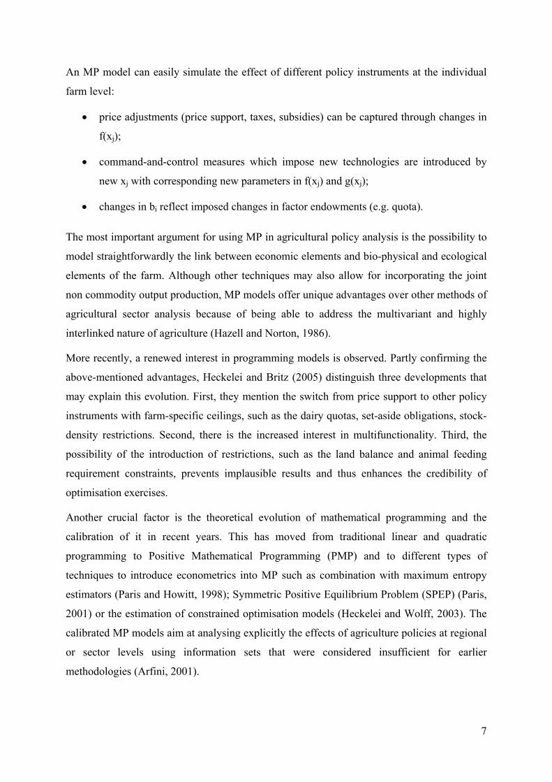
An MP model can easily simulate the effect of different policy instruments at the individual

farm level:

• price adjustments (price support, taxes, subsidies) can be captured through changes in

f(xj);

• command-and-control measures which impose new technologies are introduced by

new xj with corresponding new parameters in f(xj) and g(xj);

• changes in bi reflect imposed changes in factor endowments (e.g. quota).

The most important argument for using MP in agricultural policy analysis is the possibility to

model straightforwardly the link between economic elements and bio-physical and ecological

elements of the farm. Although other techniques may also allow for incorporating the joint

non commodity output production, MP models offer unique advantages over other methods of

agricultural sector analysis because of being able to address the multivariant and highly

interlinked nature of agriculture (Hazell and Norton, 1986).

More recently, a renewed interest in programming models is observed. Partly confirming the

above-mentioned advantages, Heckelei and Britz (2005) distinguish three developments that

may explain this evolution. First, they mention the switch from price support to other policy

instruments with farm-specific ceilings, such as the dairy quotas, set-aside obligations, stock-

density restrictions. Second, there is the increased interest in multifunctionality. Third, the

possibility of the introduction of restrictions, such as the land balance and animal feeding

requirement constraints, prevents implausible results and thus enhances the credibility of

optimisation exercises.

Another crucial factor is the theoretical evolution of mathematical programming and the

calibration of it in recent years. This has moved from traditional linear and quadratic

programming to Positive Mathematical Programming (PMP) and to different types of

techniques to introduce econometrics into MP such as combination with maximum entropy

estimators (Paris and Howitt, 1998); Symmetric Positive Equilibrium Problem (SPEP) (Paris,

2001) or the estimation of constrained optimisation models (Heckelei and Wolff, 2003). The

calibrated MP models aim at analysing explicitly the effects of agriculture policies at regional

or sector levels using information sets that were considered insufficient for earlier

methodologies (Arfini, 2001).

7

A final incentive to use MP is the close link between model elements and real world

constraints, which enhances the comprehensibility of the model and the results for policy

makers. As such, MP can be seen as a communication facilitating instrument for the various

stakeholders in a changing policy environment, in particular the farmer and the policy-maker

(Fernagut et al., 2004).

Objective: description of 3 types of MP

The introduction has, so far, mainly motivated the focus of the dissertation: farm-level

mathematical programming modelling. The rest of the dissertation is devoted to the

description, application and critical assessment of three mathematical programming

approaches, of which the choice depends on the type of problem and the availability of

historical data.

In the dissertation, a distinction is made between:

• Purely normative mathematical programming (NMP) models, that simulate an optimal

solution among possible solutions using a predefined decision rule.

• Positive mathematical programming (PMP) models, that incorporate observed

behaviour to calibrate the normative simulation behaviour.

• Econometric mathematical programming models (EMP) that use more advanced

econometric techniques to calibrate parameters used in the decision model.

The objectives of this dissertation are to describe these types of MP models in detail, to

develop tools based on the three types of programming models for agricultural policy support

and to apply the developed tools on specific cases. The applications should prove the

usefulness of the models for policy analysis and can lead to policy recommendations.

However, due to the wide variety of topics and particularities of each of the applications,

these recommendations should be looked upon separately and do not form topics for the main

conclusions of the dissertation. Instead, in the conclusion of the dissertation, an overview is

made to identify the strengths and weaknesses of the different models applied, according to

the dimensions of the applications such as the purpose of the model and the intended users.

8

The dissertation consists of a compilation of contributions in international peer reviewed

journals, books and proceedings2. To situate these different contributions into the general

structure of the dissertation, each chapter starts with a short overview and an explanation of

the role of the chapter within the general framework and ends with lessons leaned from the

modelling exercise.

The outline of the dissertation is presented in Figure 1. Chapter 1 introduces the three types of

programming models, NMP, PMP and EMP, followed by an illustration of the similarities and

differences between NMP and PMP with a simplified dairy farm model that simulates the

uptake of meadow bird management. Chapter 2 presents an application of an NMP model to

simulate the influence of management decisions on the nutrient balance of a dairy farm and

ends with a critical discussion of the strengths and weaknesses of NMP in this case. Chapter 3

elaborates on the calibration concept and the application of it in PMP. Chapter 3 presents also

the farm-level PMP model SEPALE that is used as base model in chapter 4 and 5. Chapter 3

ends with a simulation with SEPALE of the June 2003 CAP reform options and with an

evaluation of PMP and SEPALE. Chapter 4 extends the base model SEPALE with a module

to deal with sugar quota and presents simulation results of the sugar Common Market

Organisation (CMO) reform options. Chapter 5 applies the concept of EMP to the sugar

module that has been described in chapter 4. Chapter 5 also provides more detailed results for

4 groups of farms with a different reaction to the simulated sugar regime reforms. Finally, the

general conclusions of the dissertation and tries to provide more comprehensive insights for

future developments of models for agricultural policy support.

2 Each contribution is the result of collaboration with other research groups. Parts of the text of the dissertation

are written by the co-authors of these papers.

9

NMPNormative

Mathematical Programming

PMP Positive

Mathematical Programming

EMP Econometric Mathematical Programming

Chapter 1: definition and overview of:

Chapter 2: application + discussion of NMP Simulating the influence of management

decisions on the nutrient balance of a dairy farm

Chapter 3: concept + discussion of PMPIntroduction of farm-level model SEPALE

+ simulation of the MTR of the CAP

Chapter 4: application + discussion of PMP Modelling the impact of policy reforms

on Belgian sugar beet suppliers with PMP module

Chapter 5: application + discussion of EMP Modelling the impact of policy reforms

on Belgian sugar beet suppliers with EMP module

General discussion and conclusion: Comparison of methods and applications +insights on future developments of models

Figure 1. Outline of the dissertation

10

Chapter 1 Overview of the three types of programming models

This chapter starts in the introduction with the explanation of mathematical programming and

duality followed by the presentation of three mathematical programming approaches, of

which the choice depends on the type of problem and the availability of historical data. First is

shown how normative mathematical programming (NMP) can help to simulate the impact of

new activities when historical data are scarce. The second approach is Positive Mathematical

programming (PMP), which allows taking both historically observed behaviour and new

normative information into account. The similarities and differences between both approaches

are illustrated with a toy-size dairy farm model that simulates the uptake of meadow bird

management. Finally, a more advanced programming technique, Econometric Mathematical

Programming (EMP), is introduced combining the advantages of econometrics and

programming techniques.

Parts of this chapter have been published as

Buysse, J., Van Huylenbroeck, G. and Lauwers, L. (2006). Normative, positive and

econometric mathematical programming as tools for incorporation of multifunctionality in

agricultural policy modelling. Agriculture, Ecosystems & Environment, in press.

11

1.1 Introduction

Before presenting the three MP approaches that can be used, this introduction explains the

basic idea of MP and the ‘duality’. Following linear programming model in its primal form

illustrates the use of mathematical programming in agricultural economics:

max Z = ∑j c j x j (3)

Subject to:

∑j aij x j ≤ bi (4)

xj ≥ 0

where: cj is the forecasted gross margin of farm activity j,

xj is the level of farm activity j,

aij is the quantity of resource i required to produce one unit of activity j,

bi is the amount of available resource i,

i is the index of resource and j is the index of activities.

The solution of this primal model gives information on which activities should be chosen to

maximise the gross margin. The primal model provides, however, no information how to

increase the gross margin by acquiring additional resources i. Therefore, we have to calculate

the marginal value product of each resource i (in programming literature this is also called the

shadow cost of the resources).

The dual problem is the linear programming model specified to find these shadow prices λi

for the fixed resources i. We can solve thus actually two problems: the primal resource

allocation problem, and the dual resource valuation problem. The study of duality is very

important in MP because duality increases insight into MP solution interpretation (Hazell and

Norton, 1986). The dual problem can be stated as follows:

min W = ∑i bi λi (5)

Subject to:

∑i aij λi ≥ cj (6)

λj ≥ 0

The shadow costs λi found by the dual problem correspond to the Lagrange multipliers that

are used in the first-order optimality conditions of the primal MP model (also called the

Kuhn-Tucker conditions or complementary slackness conditions). Duality is here for

comprehensibility reasons illustrated for linear MP models, but it applies to non-linear models

as well.

12

The concept of duality is important and is used in all thee MP methods that are presented in

the following subsections of this chapter.

1.2 Normative mathematical programming (NMP)

1.2.1 Arguments for using NMP in agricultural policy analysis NMP has been used in agricultural economics for more than 50 years. This prescriptive type

of model starts from a decision rule of the decision maker, which determines the levels of the

different variables when aiming to optimise the objective set by the decision maker (Hazell

and Norton, 1986). Usually, this concerns utility maximisation from a private economic

viewpoint. Both the targets and the decision variables can comprise economic, ecological or

social aspects of the system, which again highlights the possibility of a multidisciplinary

approach in programming models. An extension to multi-objective and goal programming

techniques even allows finding the best compromise in the case of conflicting objectives

(Romero and Rehman, 1989).

In the NMP models, parameters of the objective function and constraints are not calibrated to

historical data. This means that for constructing an NMP model, basic knowledge of the

system is sufficient. The disadvantage is that NMP does not guarantee that the observed or

baseline data are reproduced.

McCarl and Spreen (2004) put the numerical usages of NMP into four subclasses: 1)

prescription of solutions; 2) prediction of consequences; 3) demonstration of sensitivity; and

4) solution of systems of equations. Although prescription of solutions is perceived as the

basic function of mathematical programming, it is probably the least common in practice. The

reason is that because of the normative character of NMP models, decision-makers often do

not trust the policy model results sufficiently to replace own judgement. Prediction of

consequences and demonstration of sensitivity are therefore, usually combined, more

important for agricultural policy support (Pannell, 1997). Finally, the solution of systems of

equations is similar to a technical device in empirical problems and therefore only indirectly

applicable for policy analysis.

For the prediction of consequences, the policy makers are interested in the comparison

between the currently applied policy, called the baseline, and the alternative policy options. In

order to be valid, the policy analysis model in its baseline run must reproduce the observed

situation as close as possible. Because of the lack of adequate calibration mechanisms, NMP

does not guarantee that such a validation exercise will be a success.

13

This disadvantage of NMP can be explained with the simplified NMP model illustration in

Figure 2. The graph shows the production possibilities for a farm with two crops, X1 and X2.

The objective function of the farm is to maximise its profits. The NMP iso-profit line is thus

determined by the price and cost ratios of the two crops. The optimal solution can be found by

parallel shifting the iso-profit line away from the origin. The point with the largest distance to

the origin within the convex hull of constraints is the optimum. In the case illustrated in

Figure 2, point ‘a’ is the maximum, reflecting the situation that the optimal crop mix does not

correspond to the observed production. The distance between the observed point “a” and the

optimal point is due to the fact that the values of the technical coefficients and variable costs

in the model are different from the real ones or because not all constraint are represented in

the model. This results in different ratios between prices and costs of the two crops and

creates a difference between the observed solution and the optimal solution.

Variation of the price or cost ratios causes changes in the slope of the iso-profit line. The

graph representation of the NMP decision problem also makes clear that with relatively small

changes in the iso-profit line, the corner point ‘a’ will remain the optimum. Only with a large

change in slope of the iso-profit line, the maximum jumps abruptly to corner point ‘b’.

Besides the fact that the NMP solution does not reflect the observed situation, the staircase

situation between the corner point solutions is a second disadvantage of NMP. The staircase

stituation poses more problems to regional models than to farm models because individual

farms are more likely to react abruptly than the sum of all farms from a region.

14

X1 (quantity)

X2 (quantity)

a

b

Observed productionIso-profit lineConstraints

Figure 2. Graphical illustration of a simplified NMP farm model with two activities (X1 and

X2) and a profit maximising objective function.

Despite the disadvantages, there are several motivations for continuing to apply NMP. The

first and most important one is, when confronted with new policies or farm practices, the lack

of empirical data that sufficiently describe the system in a baseline situation. Empirical data

could be unavailable because the modelled activity is very novel or when the model scope is

too detailed.

The second reason for still using NMP is the fact that one is not always interested in the

optimal situation itself neither whether it reflects baseline. The design and use of NMP can

also help to understand a problem and to discover relevant decision variables and constraining

factors. A calibration procedure may be obsolete for this case.

15

The third reason is that a number of methodological developments in the field of MP attenuate

the disadvantages mentioned above. The inclusion of more economic theory and observed

institutional and economic reality results in better validated models (Hazell and Norton,

1986). While the first applications relied on linear programming because of the available

algorithms to solve this type of problems, current models can, thanks to improved solver and

computer equipment, also include nonlinear functions, resulting in less staircase situations.

Moreover, the development of multi-objective and goal programming techniques, allowing

the trade-off between conflicting objectives, has resulted in certain areas (such as, e.g.,

modelling of water policies) in a renewed interest for NMP (see e.g. Gomez-Limon et al.,

2002; Gomez-Limon and Riesgo, 2004).

The following subsection demonstrates the applicability of NMP with an illustrative example.

1.2.2 Normative model to predict participation to meadow bird management The illustrative model tries to analyse the participation level of a farm to an agri-

environmental scheme to protect meadow birds. The agri-environmental scheme (AES), as

applied in Flanders, compensates the income loss of farmers in case they switch to more

extensive grassland management in order to protect meadow birds. The meadow bird

management implies delayed fertilisation and a lower stock density, resulting in lower grass

yield and quality. The meadow bird population can only develop in extensively managed

grassland, whereas the farmer tries to intensify the grassland management to have a higher

grass yield.

The model describes a simplified hypothetical dairy farm with the possibility to produce milk,

maize, and intensively and extensively managed grassland. Maize can be sold or used as

fodder on the farm, while grass only serves as fodder and can not be sold. The dairy farm has

revenues from the milk sold, maize sold and from the subsidies for extensively managed

grassland. The NMP model of the dairy farm maximises a profit function subject to a land

constraint, milk quota constraint and feeding constraints. The feeding constraints are based on

the Dutch VEM-DVE system (CVB, 1996). The requirements and the supply of protein are

expressed as Darm Verteerbaar Eiwit (DVE), the protein actually digested in the small

intestine, and the requirements of energy are expressed as Voeder Eenheid Melk (VEM) or

Feed Unity Milk.

16

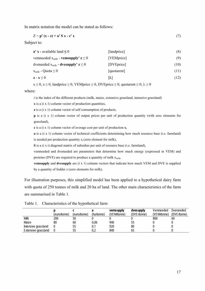
In matrix notation the model can be stated as follows:

Z = p' (x - z) + a' S x - c' x (7)

Subject to:

a' x - available land ≤ 0 [landprice] (8)

vemneeded xmilk - vemsupply' z ≤ 0 [VEMprice] (9)

dveneeded xmilk - dvesupply' z ≤ 0 [DVEprice] (10)

xmilk - Quota ≤ 0 [quotarent] (11)

z - x ≤ 0 [λ] (12)

x ≥ 0, z ≥ 0, landprice ≥ 0, VEMprice ≥ 0, DVEprice ≥ 0, quotarent ≥ 0, λ ≥ 0

where: i is the index of the different products (milk, maize, extensive grassland, intensive grassland)

x is a (i x 1) column vector of production quantities,

z is a (i x 1) column vector of self consumption of products,

p is a (i x 1) column vector of output prices per unit of production quantity (with zero elements for

grassland),

c is a (i x 1) column vector of average cost per unit of production x,

a is a (i x 1) column vector of technical coefficients determining how much resource base (i.e. farmland)

is needed per production quantity xi (zero element for milk),

S is a (i x i) diagonal matrix of subsidies per unit of resource base (i.e. farmland),

vemneeded and dveneeded are parameters that determine how much energy (expressed in VEM) and

proteins (DVE) are required to produce a quantity of milk xmilk,

vemsupply and dvesupply are (i x 1) column vectors that indicate how much VEM and DVE is supplied

by a quantity of fodder z (zero elements for milk).

For illustration purposes, this simplified model has been applied to a hypothetical dairy farm

with quota of 250 tonnes of milk and 20 ha of land. The other main characteristics of the farm

are summarised in Table 1.

Table 1. Characteristics of the hypothetical farm p

(euro/tonne) c (euro/tonne)

a (ha/tonne)

vemsupply (VEM/tonne)

dvesupply (DVE/tonne)

Vemneeded (VEM/tonne)

Dveneeded (DVE/tonne)

Milk 200 50 0 0 0 800 60 Maize 80 60 0,06 940 55 0 0 Intensive grassland 0 55 0,1 920 80 0 0 Extensive grassland 0 55 0,2 840 65 0 0

17

The product quantities x (milk) and z (maize and grassland) are the decision variables in the

model. Landprice, VEMprice, DVEprice, quotarent and λ are the dual variables in the model.

They show the increase of the objective function when the constraints become more relaxed.

The level of p, c, a, vemsupply and dvesupply are given and constant during simulation. The

level of subsidies for extensively managed grassland in matrix S is the external policy

parameter and can be changed. Changing S simulates the impact of varying compensation

levels for managing grassland extensively on the uptake of this agri-environmental scheme.

The result of the simulation exercise is presented in Figure 3. Figure 3 illustrates that the

numerical example has four corner solutions. For compensation levels lower than 200

euro/ha, the feeding requirements are filled with intensive grassland and maize. A part of the

maize is sold and there is no extensive grassland. For compensation levels from 250 to 650

euro/ha, 5 ha of extensive grassland is included in the model and used for feeding and no

maize is sold. For 700 euro/ha compensation, the milk quota is not filled and only 4 tonne of

intensive grass is produced. For 750 euro/ha and higher compensation levels, all grassland is

extensively managed.

0

50

100

150

200

250

150 350 550 750 950Extensive grassland

compensation (euro/ha)

production (tonne)

Maize

Intensivegrassland

Extensivegrassland

Milk


production of the different activities on the dairy farm

18

The normative character of the simulations implies that the model outcomes must be

interpreted as uptake potentials rather than as predicted uptake of this environmental scheme.

However, as far as these results remain close to the actual potential that can be detected and

stimulated by farm advisory experts, they also enable descriptive analyses. In any case, they

can inform decision-makers of potential reactions of farmers on incentives provided.

By introducing changes in the other parameters (c, a, vemsupply and dvesupply) that are

constant during simulation, the impact of underlying farm characteristics could be analysed.

This allows analysis of how farms with different characteristics react to the same incentives.

Finally, the model can also serve as a tool for analysing the sensitivity of the results for

changes in the decision-making environment, such as changes in market prices p or policy

interventions in other activities than the extensively managed grassland through S. As such

the model could be used as a policy impact analysis tool.

Normativity and uncertainty of these external factors, however, call for specific needs with

respect to the organisation of information production and communication of information. The

advantage of NMP in this case is that it allows for incorporating expert knowledge and (if

coupled to an attitude model) behavioural factors, which makes the prediction more realistic.

Despite the normative character of the economic potential models, they can serve as a

laboratory where the policy analyst can simulate a wide range of policy options.

1.3 Positive mathematical programming (PMP)

1.3.1 Calibration of farm-level MP models Positive mathematical programming models have been developed to overcome the normative

character of NMP. Contrary to NMP models, in PMP some parameters are adjusted to be able

to reproduce exactly a given baseline. Because this type of model reproduces observed data,

the method is called positive. The main purpose of this descriptive type of model is to explain

producer’s reactions to external changes, which makes PMP models extremely interesting for

policy makers.

19

The main argument to build PMP models is the increase in reliability through avoiding the

difference between the empirical baseline situation and the simulated baseline situation, but

also to reproduce the behaviour of farmers in their specific environment according the few

data that are available and reflecting farm decision process: use of land and production

quantity. PMP, as originally proposed by Howitt (1995a), is considered as the most widely

applied method for calibration of an MP model. In this dissertation, we describe MP

calibration in a more generalised way, of which the original PMP approach (Howitt, 1995a) is

a special case. Nevertheless, we call the more general approach also PMP, because it encloses

all published variants on PMP (for an overview, see Heckelei and Britz (2005) and Henry de

Frahan et al. (2006)).

Figure 4 uses a simplified model to explain the basic idea behind PMP and the comparison of

Figure 4 and Figure 2 illustrates the differences between NMP and PMP.

In contrast to NMP, PMP starts from the concept that the activity mix observed at the farm is

optimal and reflects the farmer behaviour considering all the constraints (visible and not), the

production level, the technology and the hidden cost of farm choice relating the used

technology and land allocation.

The main idea is that it is sometimes easier to reproduce a proxy of the technology than the

technology itself and that the cost function (alias the cost of the technology) is the dual of the

production function (alias the technology) and, thus, a proxy for the technology. Because it is

impossible for the modeller to find out information related to used technology and production

cost, a non linear cost function able to capture the variable cost associated with the dual price

of the constrained factors and the activity level is calibrated. In the example in Figure 4, a

convex non-linear cost function is put into the profit function resulting in a concave total

profit function. The parameters of the objective function are adjusted to reproduce exactly the

baseline.

20

Because of the calibration and the non-linear function in the model, PMP avoids two of the

drawbacks of NMP: problems of reproducing the baseline and the staircase situations. It is

clear that the positive attribute is not an objective but instead a specific characteristic of the

methodology, as in econometric methodology, and the calibration phase is the step adopted in

order to reach the character of a positive model. Of course the main goal of this type of

models is to simulate farm behaviour according to some policy scenario referred to real farms

and not to hypothetical farms. In this sense the normative character is needed but in a second

step and for this reason it is possible to define these models as positive-normative models.

The possible numerical use of PMP is, however, more limited than NMP. PMP can not be

used to find prescriptive solutions for farms about their optimal activity mix because PMP

assumes their choice is optimal. On the other hand, PMP is very practical for prediction of

consequences and demonstration of sensitivity as long as enough empirical data are available

for calibration of the model.

X1 (quantity)

X2 (quantity)

a

b

Observed productionIso-profit lineConstraints

Figure 4. Graphical illustration of a PMP simplified farm model with two activities (X1 and

X2) and a profit maximising function

The first prerequisite for building a PMP model is a proper definition of the model. Definition

of the model comprises the choice of the functional form of the objective function and

constraints and the definition of endogenous variables, exogenous variables and parameters to

be calibrated.

21

Starting from the final simulation model we have in mind, the optimality conditions are

derived for calibrating the model. Both the necessary and the sufficient conditions for an

optimum must be satisfied. For an MP model with a non-linear objective function and linear

constraints, the so-called Kuhn-Tucker conditions form the necessary conditions. Moreover,

these Kuhn-Tucker conditions are also sufficient for a maximisation problem if the objective

function is quasi-concave with quasi-convex constraints or for a minimisation problem if the

objective function is quasi-convex with quasi-concave constraints (Mills, 1984). Therefore,

the Kuhn-Tucker conditions form the set of calibration equations.

For calibration, enough empirical data should be gathered to have zero degrees of freedom in

the calibration equations. In practice, however, data availability is often not sufficient

resulting in the need for using additional (and sometimes ad hoc) assumptions. Various

authors have proposed different types of assumptions. The original, and until now most

applied PMP version (Howitt, 1995a), uses in a first phase an additional MP model with

calibration constraints to assign the unknown dual values of the resource constraints. This

approach assigns the highest possible value to the dual variables of the resource constraints

that still make a perfect calibration possible3. For an overview of the variations on the original

approach by Howitt (1995a), we refer to Henry de Frahan et al. (2006). Instead of taking the

highest possible value for the duals of the resource constraints, other authors (Judez et al.,

2001; Heckelei and Britz, 2005; Henry de Frahan et al., 2006) suggest using as much as

possible available information about prices of resource constraints as a proxy for the dual

values.

However, not all authors agree to use external values (as proxy of dual values) for calibration

of an MP model by PMP. In particular Paris (1997, 2001), Paris and Arfini (2000) and Paris

and Howitt (1998), suggest to avoid external values in order to avoid “contamination” of the

observed data. Their concern is related to the fact that external values allow to calibrate the

model according the Langrangian function and the obtained variable cost, but don’t represent

the real “internal” dual value for a given specific farm.

3 The dual value of the resource constraints of phase 1 of original PMP is the highest possible if it is assumed

that the total cost correspond to the sum of the observed accounting costs used in phase 1 of PMP and some

potential unobserved costs. These observed accounting cost define then a minimum for the calibrated total cost

function.

22

To demonstrate the principles of PMP, we transform in the next subsection the illustrative

NMP model of section 1.2.2 into a PMP variant.

1.3.2 PMP model to predict participation to meadow bird management To demonstrate the PMP approach for the same problem as in section 1.2.2, we suppose that

we already have some observations of farms participating to the meadow bird management

program. Table 2 contains empirical data that could be gathered from management programs

that are in place for some time and are adopted by two farms. The parameters on costs, prices

and yields of both farms are the same as in Table 1, except that Farm 2 has 10% higher costs.

The NMP model presented in the previous section could then be validated against these

empirical data. The validation results show that the NMP model of section 1.2.2 does not

reproduce the baseline.

Table 2. Empirical data of two hypothetical farms under the assumption of a 300 euro/ha

compensation for extensive grassland

Farm 1 Farm 2 Observed* Simulated by NMP* Observed* Simulated by NMP* Production Milk 200 200 250 236 Maize 133 54 133 73 Extensive grassland 100 117 110 0 Intensive grassland 10 25 5 136 Self consumption Maize 100 54 133 73 Extensive grassland 100 117 110 0 Intensive grassland 10 25 5 136

23

Because of the availability of empirical data, the illustrative model can be turned into a PMP

variant. The objective function consists again of a profit function but now it includes a

quadratic functional form for its cost component. In matrix notation, this gives:

Z = p' (x - z) + a' S x - x' α x / 2 - β' x (13)

where:

α is an (i x i) diagonal matrix of quadratic cost function parameters,

β is an (i x 1) column vector of linear cost function parameters.

Model (13) is extended with the same land, quota and feeding constraints as model (7). Again,

the production quantities x and z of the model are the decision variables. Calibration

determines the cost function parameters in the matrix α and vector β and the cow productivity

parameters: VEMneeded and DVEneeded. Prices (p) and Subsidies (S) are exogenous to the

model.

This model (13) has a concave objective function with convex constraints. Now, the

calibration conditions are derived from the Kuhn-Tucker conditions of model (9). In its

Langragian form this model can be written as follows:

L = p' (x - z) + a' S x - x' α x / 2 - β' x - landprice (a' x - available land) - VEMprice

(vemneeded xmilk - vemsupply' z) - DVEprice (dveneeded xmilk - dvesupply' z) - quotarent

(xmilk - Quota) - λ (z - x)

For comprehensibility reasons, only the relevant equations for calibration are given here in

algebraic notation:

(∂L/∂VEMprice) VEMprice = 0 ⇒ (for a strictly positive VEMprice)

∑i zi vemsupplyi = VEMneeded xi (14)

(∂L/∂DVEprice) DVEprice = 0 ⇒ (for a strictly positive DVEprice)

∑i zi dvesupplyi = DVEneeded xi (15)

(∂L/∂zi) zi = 0 ⇒ (for every strictly positive zi)

-pi - λ + VEMprice vemsupplyi + DVEprice dvesupplyi = 0 (16)

(∂L/∂xi) xi = 0 ⇒ (for every strictly positive xmaize, xintensivegrass, xextensivegras)

pi + λ + ai si - αi xi - βi - ai landprice = 0 (17)

substituting (16) in (17) results in following calibration equations for every fodder crop:

VEMprice vemsupplyfodder + DVEprice dvesupplyfodder + afodder sfodder – αfodder xfodder

- βfodder - afodder landprice = 0 (18)

(∂L/∂xmilk) xmilk = 0 ⇒ (for the strictly positive xmilk)

pmilk + amilk smilk - αmilk xmilk - βmilk - VEMprice vemneeded - DVEprice dveneeded = 0 (19)

24

The parameters VEMneeded and DVEneeded can be assigned from equations (14) and (15).

To calibrate αi and βi, the observed average cost c can be used as additional information in the

calibration as follows (in algebraic notation for every activity i):

ci = αi xi / 2 + βi (20)

In order to obtain zero degrees of freedom in the calibration equations (18), (19) and (20),

additional data have to be gathered for the dual variables landprice, VEMprice and DVEprice.

If we suppose a landprice of 250 euro/ha on Farm 1 and 200 euro/ha on Farm 2, a VEMprice

of 0.070 euro/kVEM and a DVEprice of 0.268 euro/kg DVE, α and β can be calibrated as

follows:

αfodder = 2 (VEMprice vemsupplyfodder + DVEprice dvesupplyfodder + afodder sfodder - afodder landprice - cfodder) / xfodder (21)

αmilk = 2 (pmilk + amilk smilk - VEMprice vemneeded - DVEprice dveneeded - cmilk) / xmilk (22)

βi = ci - αi xi / 2 (23)

Once model (13) is calibrated, changing the exogenous variables p and S can simulate

different policy alternatives. Figure 5 shows the response of the two hypothetical farms on an

increasing compensation for meadow bird management. The difference in results for both

farms can be explained by differences of the economic situation between the farms. Farm 1

has, in its baseline, excess fodder production resulting in sales of maize. An increase in

subsidies for extensive grassland first reduces the production and the selling of maize. For

compensation levels higher than 800 euro/ha of extensive grassland, Farm 1 has almost no

excess fodder production anymore and, therefore, the linear increase in extensive grassland

slows down. Farm 2 has in the baseline no excess fodder production. For this reason,

switching to meadow bird management is more difficult.

25

0

5

10

15

20

25

30

100 500 900Extensive grassland

compensation (euro/ha)

production (tonne)

Farm 1

Farm 2


production of the extensively managed grass on the dairy farm

The illustrative example shows very well that PMP is able to simulate different reactions

based on the observed empirical data. Not only PMP proves its value to analyse the

differences between farms. But also, when bringing the information of a sample of individual

farm models together, PMP allows to build sector models (see e.g. Buysse et al., 2005a).

Moreover, such a model can implicitly simulate transactions between farms and individual

farmers’ behaviour, depending on their situation and past behaviour. This results in more

balanced and realistic simulations of intended policies.

The PMP approach is already applied by various authors for simulating policy responses.

Own research with PMP has resulted in the so-called SEPALE model for Belgian agriculture

with applications on the June 2003 CAP reform (including modulation of payments) (Henry

de Frahan et al., 2006) and on the sugar reform (Buysse et al., 2005a) (see also chapter 3.5

and Chapter 4).

26

These applications highlight that the main advantage of PMP, namely that it allows prediction

based on past observations of the cost function and thus real farmer’s behaviour. It

incorporates individual data, derived from real accountancy data. As such, it allows to

differentiate results according to farm types, farm size or farm location. This aspect becomes

important for policy analysis evaluation because it allows giving to public stakeholder and

policy maker a realistic picture on the effects of a given policy using data that they know.

Also, the cost of the analysis is relatively small because it is often based on databases already

available (as FADN) and it is not necessary specific interviews on farm holdings. So, the

unique cost is related to the development of the model. However, the calibration of cost or

production functions of activities remains difficult when no real observations are available

(e.g. limited past uptake of AES or multifunctional systems). Another disadvantage is that

although the farm-based approach opens perspectives for modelling farm interactions, it

remains difficult to incorporate the institutional rules and settings.

PMP as presented above requires zero degrees of freedom in the calibration equations. As a

consequence, the amount of data that must be gathered is very high or the number of

parameters that can be assigned during calibration is limited. Due to this limited number of

parameters, PMP models usually have a very simple functional form. When modelling

agricultural policies, the number of parameters and the functional form are often too

restrictive to capture the complex farmers’ and system behaviour. Motivated by these

shortcomings of PMP, new approaches are developed in order to answer PMP critiques and to

improve policy analysis models. In particular, as briefly discussed in the next section,

econometric mathematical programming seems a promising avenue to improve the modelling

practice.

27

1.4 Econometric mathematical programming (EMP)

The limitation of having zero degrees of freedom in the optimality conditions puts a lot of

restrictions on the flexibility of the functional form of the model4, a very heavy burden on the

data collection, or both. The approach introduced by Heckelei and Wolff (2003) is, however,

in interesting alternative. Heckelei and Wolff suggest estimating the parameters of the

programming model by using the optimality conditions as the set of estimation equations. Due

to the use of the optimality conditions, the estimated model is able to reproduce the baseline

correctly. After the estimation of the parameters, the programming model can be used to do

simulations and scenario analysis. This combination econometrics and mathematical

programming models creates a new field of empirical investigation, which we would like to

call econometric mathematical programming (EMP).

The development of MP is less than econometrics focussed on descriptive analysis. As shown

above, descriptive analysis is therefore probably the weakest element of MP models. MP has,

however, advantages for explorative research of innovation and radical changes of policy

instruments within a context of resource constraints. On the other hand, limitations of

econometric analyses include a large data requirement and the inability of the model to deal

with changes in the underlying economic structure (Hazell and Norton, 1986).

In the case no behavioural data are available, only NMP can be applied, which uses then data

from literature based on experimental data. But in the cases of sufficient data availability,

modelling should take full benefit of the advanced techniques in descriptive analysis of

econometrics and of the possibility to introduce changes in the underlying economic structure

through the mathematical programming side of the approach.

4 The number of parameters that can be identified during the calibration process of PMP models is limited.

28

The advantage of an MP model is that it is able to cope with variations in land availability,

introduction of new or alternative technologies, production quota, fallow restrictions and

environmental regulations. These changes in economic structure are gaining importance when

radically new policy mechanisms are applied. This is observed in the CAP where price

support has shifted over coupled direct payments to decoupled direct payments. Now,

multifunctionality-based intervention introduces the coupling of payments to non-commodity

outputs, which again leads to another economic logic and behaviour. Relying on a

combination of econometrics and programming is therefore perceived as taking the best of

both previous approaches with, on the one hand, the possibility to take into account the past

behaviour and on the other, opening the possibility of supplementing the econometric analysis

of this past behaviour by normative information on adaptation to new economic realities.

The combination of econometrics and programming models is not new. In order to obtain

more realistic simulation behaviour, the objective function or the constraints are often

supplemented by externally estimated functions or parameters. This introduces, however,

difficulties or even inconsistencies (Heckelei, 2002). The most obvious example of such

inconsistencies is the use of externally estimated supply elasticities to build a supply function

in a programming model, such as, e.g., in Helming et al. (2001). The econometric estimation

of supply elasticities implicitly takes all the limitations faced by the farmer into account, e.g.

among others the land constraint. If this supply function is appended with additional

constraints in the programming model, such as the land constraint, the simulation results will

not reproduce the original externally estimated supply elasticities. As a consequence, the

underlying structure of the model reflects the constraints twice: once in the econometric

estimated supply elasticities and once in the constraints explicitly specified in the model.

There exist approaches for getting around this hitch (Heckelei, 2002), but it is more useful to

directly apply EMP, meaning that the parameters of objective function and constraints are

simultaneously estimated. In this way, the fact that certain resources (such as land) are limited

will not be reflected anymore in the simultaneously estimated supply function.

Using EMP for agricultural models has two advantages. First, the limitations of the functional

form, inherent to many PMP applications, are attenuated. Second, new activities can be

introduced based on estimated functions. We can explain these advantages with our example

of the previous sections.

29

The PMP model of previous section has a cost function with two parameters per activity. An

application of EMP, based on observations of several farms or for several years, permits

choosing a more flexible functional form. Given these additional parameters in the cost

function, the model would capture better the behaviour and attitude of the different farmers.

The second advantage of EMP concerns the innovative aspects of recent policy developments

in agriculture. If data exist across several farms with different intensity of grassland

management, a relationship could be estimated between intensity of management and the

costs, yields and revenues of grassland in an EMP model. Given this relationship, the

reactions of farmers to a meadow bird management program can be simulated, even if there

are no observations of participating farmers.

Different to the NMP approach, EMP is calibrated and can use a function estimated on the

calibration data for the relation between management intensity and the yield. The NMP model

is not calibrated and uses literature data for the yield of grassland. Different to the PMP

approach, EMP allows simulating meadow bird management without actual data on

participating farmers while the PMP model of section 1.3.2 needs observations of

participation.

1.5 Conclusions

This chapter has described the three mathematical programming approaches that are used and

applied in the next chapters of this dissertation. The similarities and differences between the

approaches are illustrated with a toy-size dairy farm model that simulates the uptake of

meadow bird management. This chapter gives already some indications on the choice of

method for a research task at hand. The toy-size model has shown that this choice depends on

the type of problem and the availability of historical data. NMP can be applied when

historical data are scarce, while PMP and EMP allow taking both historically observed

behaviour and new normative information into account. EMP is more robust and theoretically

correct than PMP due to the combination of the advantages of econometrics and programming

techniques. EMP requires, however, more resources to develop than PMP.

These observations and more experiences with the three MP approaches are further developed

in the next chapters of the dissertation.

30

Chapter 2 An application of farm level NMP: Simulating the influence of management decisions on the nutrient balance of dairy farms

The purpose of chapter 3 is to illustrate an application of an NMP model. The dairy farm

model, described in this chapter, is originally developed by Geert Jacobs and Guido Van

Huylenbroeck to simulate the willingness to accept extensive grassland management on

Flemish dairy farms. In this chapter the original model is adapted and improved to be able to

make the simulation exercise presented below. For this study the model was also submitted to

a new validation exercise.

The application evaluates the influence of management decisions on the nutrient balance of

dairy farms. Three farm systems have been simulated: zero grazing, winter milk and summer

milk. From the simulated farm systems the zero grazing farm has in all scenarios the lowest N

- surplus. The winter milk farm system has a higher N - surplus than zero grazing but lower

than the summer milk farm system. The results further indicate the positive effects of maize

feeding in addition to grazing. More maize in the ration is especially good to lower the N -

surplus during the grazing period in the summer. The benefits of more maize in the ration

decrease when the fertilizer application rates decrease.

Parts of this chapter have been published as:

Buysse, J., Van Huylenbroeck, G., Vanslembrouck, I. and Vanrolleghem, P. (2005).

Simulating the influence of management decisions on the nutrient balance of dairy farms,

Agricultural Systems, 86(2): 333-348.

31

2.1 Introduction

There is a growing public concern about the increasing nitrate concentration in drinking water

reserves and about the distortion of aquatic ecosystems through eutrophication (Commission

of the European Communities, 2002). Excessive nitrogen surpluses can indeed pose a threat

on the environment, leading to pollution of water, air and soil (Pau Vall and Vidal, 1999).

This has led to the nitrates directive (91/676/EC) of the European Union (EU). This directive

aims to protect water from pollution by nitrogen from agricultural resources. In EU countries

the major source of nitrogen is mineral fertilizer, while especially in regions of high livestock

density, animal manure remains very important. In Belgium and the Netherlands, livestock

manure is responsible for more than 50% of the nitrogen inputs on the agricultural land (Pau

Vall and Vidal, 1999).

Based on agricultural statistics, it can be calculated that the contribution of cattle in the total

manure production in Flanders accounts for 47% of nitrogen and 38% of phosphorus. The pig

and poultry sector contribute 39 and 11%, respectively, for nitrogen and 45 and 15%,

respectively, for phosphorus (Deuninck et al., 2001). Dairy cattle produce approximately half

of the cattle’s manure. In the Netherlands too, the dairy sector is an important source of

pollution. Dairy farming is responsible for 45 % of the phosphate surplus and 60 % of the

nitrogen losses (Van Bruchem et al., 1999). Consequently, in countries as Belgium and the

Netherlands, where intensive animal production systems have been developed, a more

efficient utilization of dietary nitrogen in dairy farming has a positive impact on the reduction

of environmental pollution.

Michiels et al. (1998) have compared nutrient balances of 41 Flemish farms. This research

has indicated that there are large differences in nutrient use efficiency and that possibilities

exist to increase environmental efficiency by changing farm management. Two main

approaches have been suggested: (i) an optimisation of the N-utilisation at plant level and (ii)

the reduction of N-excretion at animal level. The first approach aims at an optimal application

of chemical fertilizer and manure on the land and consequently an adapted choice of crops.

The second approach is to optimise the feed mix of the cow in order to increase the nutrient

use efficiency at cow level. Both strategies are important but do mutually influence each

other. One measure cannot simply be adjusted to another measure (den Boer, 1999 and

Thornton and Herrero, 2001). Therefore, in this study a dynamic simulation model, simulating

daily plant and animal production, is used to measure the overall impact of management

decisions on the nutrient surplus at farm level.

32

The chapter is organised as follows. In Section 2, the model is described. Section 3 gives

some insight in the validation of the model and is followed by a discussion of the results in

section 4. Finally section 5 and 6 deal with the discussion and the main conclusions.

2.2 The simulation model

The basic model and underlying mathematical relations is based on earlier work at the

department of agricultural economics of Ghent University and is also published in Van

Huylenbroeck et al. (2000).

The basic idea behind the use of the model for this application is to describe the N and P cycle

at farm level based on relationships described in literature. This combined information makes

it possible to analyse the overall effect of management decisions on a dairy farm.

The model is based on (i) nitrogen-grassland relations described by Thornley and Johnson

(1990), (ii) feeding requirements from Jarrige et al. (1988) and CVB (1996), and (iii) lactation

functions from Wood (1967) and Wood (1977). These relations allow for calculation of

animal and plant production on a daily basis.

33

2.3 General model

Figure 6 gives a schematic representation of the model, showing how the model combines

both plant and animal level.

feed uptake cattle production

fodder crop production (grass and maize)

Energy requirement Protein requirement

Final products

Silage

Roughage

Cattle characteristics Farm management

characteristics

requirements of the cattle

purchased roughageand concentrates

MINERAL CYCLE manure

NH3-losses

Organic fertilizer

Compound fertilizer Mineral losses

Figure 6. Relationship between different modules in the model

The simulation model was originally implemented in Matlab code. For performance and

interface reasons it has been rewritten in Delphi code with the additional benefit that it can

also be used as a standalone simulation program. The disadvantage of using Delphi is that

there is no optimisation algorithm standard available as is the case in, e.g., GAMS (General

Algebraic Modelling System: http://www.gams.com).

In the following sections the model is described in more detail. First the animal production is

explained, then the grazing strategy and finally some nutrient cycling aspects.

34

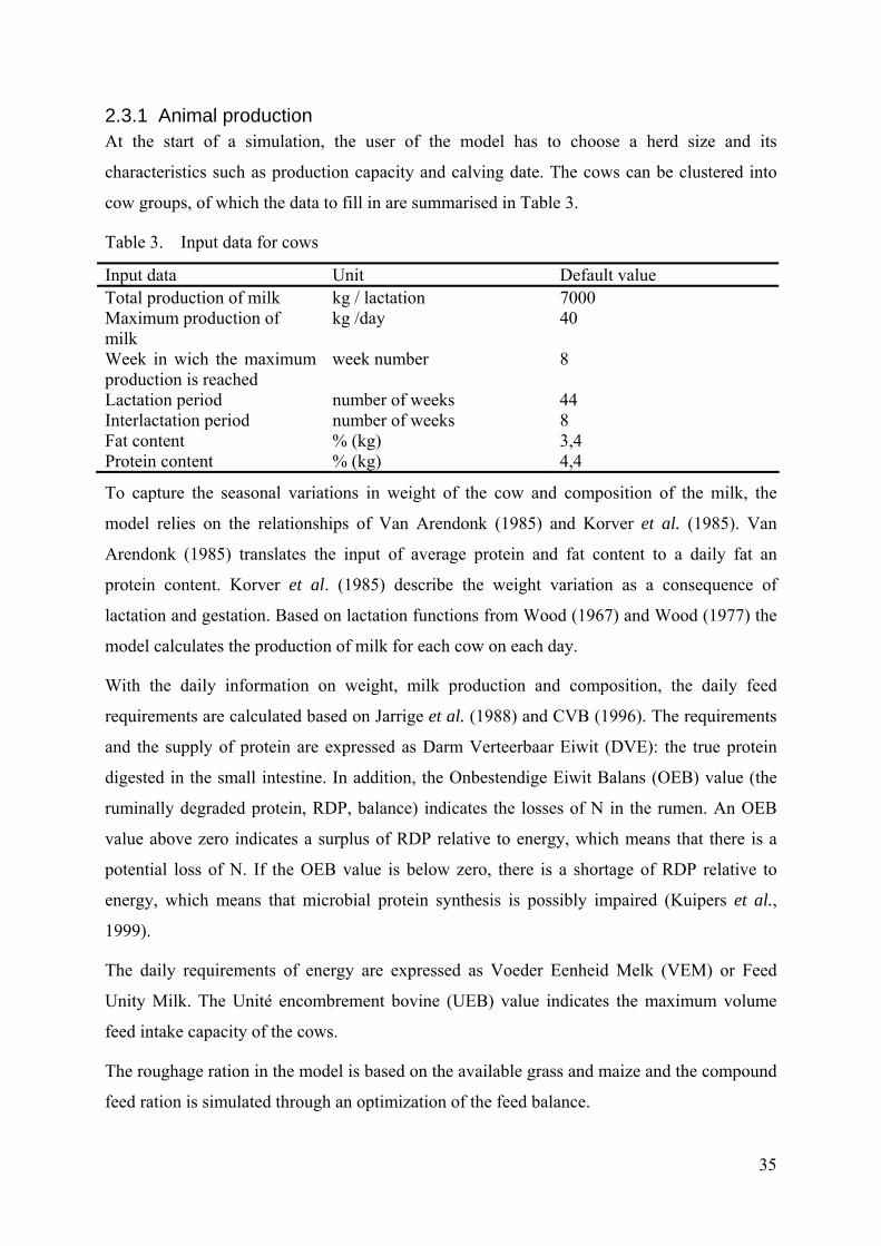
2.3.1 Animal production At the start of a simulation, the user of the model has to choose a herd size and its

characteristics such as production capacity and calving date. The cows can be clustered into

cow groups, of which the data to fill in are summarised in Table 3.

Table 3. Input data for cows

Input data Unit Default value Total production of milk kg / lactation 7000 Maximum production of milk

kg /day 40

Week in wich the maximum production is reached

week number 8

Lactation period number of weeks 44 Interlactation period number of weeks 8 Fat content % (kg) 3,4 Protein content % (kg) 4,4

To capture the seasonal variations in weight of the cow and composition of the milk, the

model relies on the relationships of Van Arendonk (1985) and Korver et al. (1985). Van

Arendonk (1985) translates the input of average protein and fat content to a daily fat an

protein content. Korver et al. (1985) describe the weight variation as a consequence of

lactation and gestation. Based on lactation functions from Wood (1967) and Wood (1977) the

model calculates the production of milk for each cow on each day.

With the daily information on weight, milk production and composition, the daily feed

requirements are calculated based on Jarrige et al. (1988) and CVB (1996). The requirements

and the supply of protein are expressed as Darm Verteerbaar Eiwit (DVE): the true protein

digested in the small intestine. In addition, the Onbestendige Eiwit Balans (OEB) value (the

ruminally degraded protein, RDP, balance) indicates the losses of N in the rumen. An OEB

value above zero indicates a surplus of RDP relative to energy, which means that there is a

potential loss of N. If the OEB value is below zero, there is a shortage of RDP relative to

energy, which means that microbial protein synthesis is possibly impaired (Kuipers et al.,

1999).

The daily requirements of energy are expressed as Voeder Eenheid Melk (VEM) or Feed

Unity Milk. The Unité encombrement bovine (UEB) value indicates the maximum volume

feed intake capacity of the cows.

The roughage ration in the model is based on the available grass and maize and the compound

feed ration is simulated through an optimization of the feed balance.

35

At the start of the simulation, the user specifies the total area and the crops that are cultivated.

Depending on the selected grazing system, the grazing season is simulated in order to fulfil

the requirements of the cattle. The excess grass production is mowed and ensiled for the

winter period. At the beginning of the winter period the available feedstock determines the

ration for the winter. This means that the winter roughage ration can be changed in the model

in two ways. The first way is to simulate a different summer situation. Selecting a grazing

system with more maize feeding during the summer period results in lower maize and more

ensiled grass availability for the winter period. The second way to change the winter ration is

changing the share of the crops cultivated. This modelling approach represents the actual

decision making process of farmers. At the beginning of the season, a farmer decides the feed

crop plan for the next year. Depending on the yields, he can adjust the ration for the cows in

order to minimize roughage surpluses at the end of the year.

To balance the feed requirements, the daily amount of compound feed is simulated through a

linear programming optimisation for each day. A least cost composition fulfilling the energy

and protein requirements is determined for each cow based on the assumption that a farmer is

able to compose a cow dependent compound mixture. This is actually representing the

situation when a feeding computer is used.

The compound feed plays two roles. It can on the one hand, supply additional energy and on

the other hand, correct the protein content and OEB balance. The optimisation of the

compound feed module can be represented as follows:

Minimize ∑i compound_input i * compound_price i

Subject to

∑i compound_input i * OEBcontent i ≥ 0 - OEBroughage

∑i compound_input i * VEMcontent i ≥ VEMneeded - VEMroughage

∑i compound_input i * DVEcontent i ≥ DVEneeded - DVEroughage

where:

i is the index of 6 types of compound feed.

2.3.2 Grazing strategy The grassland production is based on nitrogen-grassland relations described by Thornley and

Johnson (1990) and a rotational grazing strategy with the number of rotation days as external

variable.

36

dWdt

RGR W RGR WW

= −maxmax

max

2

(24)

where W is the grass yield (kg ha-1) and RGRmax is the maximum relative growth per day,

Wmax is the maximum attainable grass yield, and t is the time. After transformation of RGRmax

and substituting tmaxGR, the day that the maximum growth rate is reached, by a quadratic

function of tstart and the N-input, to capture the influence of the starting date of the growing

season and the N-fertilisation, the following non-linear algebraic expression is obtained from

the original differential equation:

( )( ) (( ) ) ⎟⎟⎠

⎞⎜⎜⎝

⎛

+++++

=−++++ ttCtCCtCtCC

STARTSTARTSTARTSTARTSTARTSTARTetCtCC

NCNCCW 2

9872

65411

)(4

2654

2321 (25)

in which C1 - C9 are coefficients fitted to the data, tstart the day the growing season starts, N the

units of applied nitrogen in kg and t the observed calendar day. The model has been fitted on

the basis of experimental data obtained from Behaeghe (1979) and Asijee (1993) for normal

growth conditions and from Nevens and Reheul (1998) for the grass growth under

management constraints. The resulting model permits to simulate the daily grass growth under

Flemish weather conditions in function of the N-fertilisation, the N-application date, the

mowing date and a possible delay in the growth due to seasonal and other factors.

The parcel size for the rotational management is simulated from the grass requirement of the

cattle on the first grazing day. Based on herd size, the model calculates what parcel size is

necessary to graze the herd during the number of days of the selected grass rotation strategy.

The grassland requirement depends on the feeding strategy. The user of the model can choose

between feeding a fixed amount of maize, maximization of grass feeding or time dependent

maize feeding. In the latter the user can define a starting quantity and a final quantity of maize

input. The model then calculates a linear daily increase of maize feeding.

Grassland production that is not used for grazing is mowed. Because the number of mowing

cuts has an influence on the total yield of the grassland (Verbruggen, 2000), the model

optimises the mowing regime to achieve maximum yield. As the grass yield is a non-linear

function of time and N-gift, the mowing regime is optimised with the Praxis-algorithm (Brent

1973) that supports non-linear optimisation.

37

2.3.3 Nutrient cycling aspects The nutrient balance of a farm is the difference between the nutrient inputs and nutrient

outputs at farm level. The most important inputs bought by the farmer are fertilizers,

compound feed and, in case of shortage, extra forage. At the output side the nutrient content

of milk, meat and potential surplus of forage are accounted for. N deposition is not considered

because this is constant over all scenarios and has thus no influence on the conclusions.

The amount of compound fertilizer needed is calculated as the difference between the need of

soil N and P of the crops and the amount applied through available manure. The amount of N

and P in the manure is calculated as the difference between the cow’s intake of N and P and

its output, both at cow level. The calculated amount of N is multiplied by a efficiency factor

and a summer and winter manure coefficient of 20% and 80% respectively. The efficiency

factor (z) indicates that 1/z kg N in manure is necessary to replace 1 kg N in compound

fertilizer for the same yield. Schils and Snijders (1988) report a efficiency factor of 56%. The

summer and winter manure coefficients take into account that only a part of the N excreted by

the animals is finally available for spreading on the land. In the winter there are mainly

storage losses. During the summer only a part of the faeces and urine is captured as manure in

the stable. The largest part is disposed directly on the land by the cows. Standard the

programme applies a summer and winter manure coefficient of 20% and 80% respectively.

Because other studies indicate that in practice there is a very large variation of these

coefficients, the results section contains a sensitivity analysis of these values. Schreuder et al.

(1995), for instance, do not take the N surplus during summer into account. Nevens and

Reheul (1998) found that the short-term fertilization effect of N in manure is only 15% while

the long-term effect is 60%. Lewis et al. (2002) have shown that the effect strongly depends

on the application date and form of the manure.

2.4 Validation

The model results are compared with recent data of farms participating in a nutrient balance-

monitoring project (Table 4) (Mulier et al., 2003). These farms do not reflect average results

of Flemish dairy farms, because they are encouraged to decrease nutrient surpluses.

38

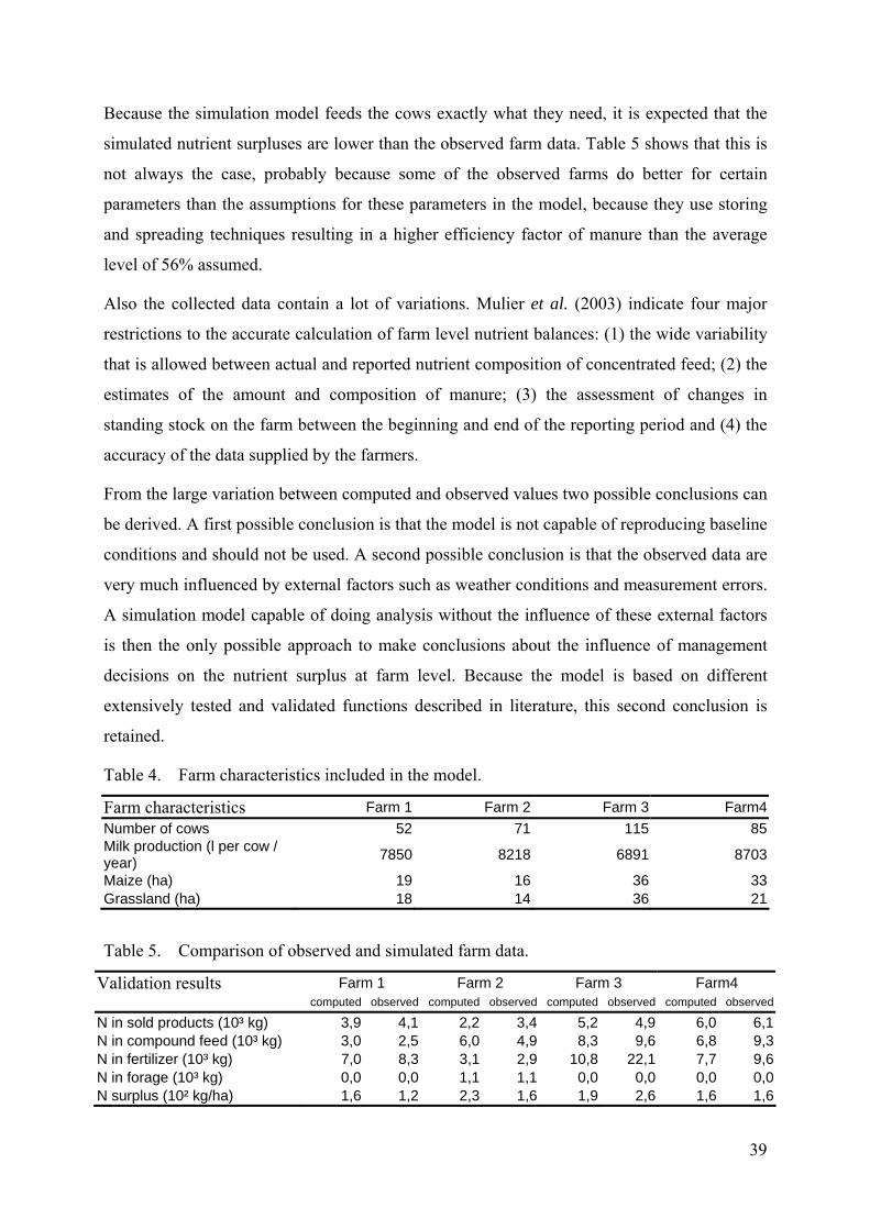
Because the simulation model feeds the cows exactly what they need, it is expected that the

simulated nutrient surpluses are lower than the observed farm data. Table 5 shows that this is

not always the case, probably because some of the observed farms do better for certain

parameters than the assumptions for these parameters in the model, because they use storing

and spreading techniques resulting in a higher efficiency factor of manure than the average

level of 56% assumed.

Also the collected data contain a lot of variations. Mulier et al. (2003) indicate four major

restrictions to the accurate calculation of farm level nutrient balances: (1) the wide variability

that is allowed between actual and reported nutrient composition of concentrated feed; (2) the

estimates of the amount and composition of manure; (3) the assessment of changes in

standing stock on the farm between the beginning and end of the reporting period and (4) the

accuracy of the data supplied by the farmers.

From the large variation between computed and observed values two possible conclusions can

be derived. A first possible conclusion is that the model is not capable of reproducing baseline

conditions and should not be used. A second possible conclusion is that the observed data are

very much influenced by external factors such as weather conditions and measurement errors.

A simulation model capable of doing analysis without the influence of these external factors

is then the only possible approach to make conclusions about the influence of management

decisions on the nutrient surplus at farm level. Because the model is based on different

extensively tested and validated functions described in literature, this second conclusion is

retained.

Table 4. Farm characteristics included in the model.

Farm characteristics Farm 1 Farm 2 Farm 3 Farm4Number of cows 52 71 115 85Milk production (l per cow / year) 7850 8218 6891 8703

Maize (ha) 19 16 36 33Grassland (ha) 18 14 36 21

Table 5. Comparison of observed and simulated farm data.

Validation results Farm 1 Farm 2 Farm 3 Farm4 computed observed computed observed computed observed computed observed

N in sold products (10³ kg) 3,9 4,1 2,2 3,4 5,2 4,9 6,0 6,1N in compound feed (10³ kg) 3,0 2,5 6,0 4,9 8,3 9,6 6,8 9,3N in fertilizer (10³ kg) 7,0 8,3 3,1 2,9 10,8 22,1 7,7 9,6N in forage (10³ kg) 0,0 0,0 1,1 1,1 0,0 0,0 0,0 0,0N surplus (10² kg/ha) 1,6 1,2 2,3 1,6 1,9 2,6 1,6 1,6

39

2.5 Simulation results

As indicated, the model is used to simulate the influence of management decisions on the

nitrogen surplus. Simulations are done for a farm with the following characteristics:

• 40 Cows

• A production of 7000 kg of milk per cow in the first lactation and 8000 kg per cow from

the second lactation on.

• The grazing season starts April 27th and runs until October 2nd (this is an average season

under Flemish conditions).

Because calving dates influence the age, weight and feed ration of the calves in a one-year

simulation period, young stock is not simulated for this application. This facilitates the

comparisons between different simulation scenarios.

The period between two calving dates is assumed to be one year. Three farm systems have

been simulated. In the winter milk farm system, cows are calving in October while in the

summer milk farm system the calving date is the first of April. In addition a zero grazing farm

system has been simulated, with a calving date the first of April.

The acreage of the farm systems is 19 ha for the summer and winter milk farm systems. The

zero grazing farm system needs less land to be self-sufficient in fodder crops and has

therefore only 17 ha of land.

For these three farm systems results are simulated for different summer rations and varying

grass – maize ratios. They are described in the next two sections. Afterwards a comparison is

made between the three farm systems and results are tested for sensitivity on fertilizer

application rates and the summer and winter manure coefficients.

2.5.1 Influence of the summer ration To analyse the effects on the N-surplus of maize input during the grazing period, different

levels of maize feeding during the summer period are simulated. Figure 7 gives the results for

the summer milk and winter milk farm systems for three different levels of maize feeding.

The results indicate that the winter milk farm system and a higher maize input during the

summer lower the N-surplus. The fertilizer application rates for this simulation are 300 kg

N/ha for grassland and 200 kg N/ha for maize.

40

200

220

240

260

280

300

320

340

360

1 - 2 2 - 4 3 - 6 maize feeding during

summer (kg/day)

N surplus(kg/ha)

Figure 7. Influence of the summer ration on the N – surplus of the ■ summer milk farm

system and the □ winter milk farm system

Different reasons explain these results. A first reason is that more maize during summer and

more milk production during winter result in less grazing. As grazing is less efficient than

mowing with equal amount of N-fertilization, this results in a lower N-surplus for the

wintermilk farm system. Secondly, mowing gives a more N-rich winter feed resulting in

better N-recycling, as can be derived from the difference between the winter (80%) and

summer (20%) manure coefficient. Thus, the N-surplus at cow level is 60% better recycled

during winter than during summer. Another reason is the OEB - balance. Grazing without

maize feeding results in a surplus of RDP relative to energy and a positive OEB - balance. A

positive OEB - balance indicates that more N - losses occur. Because maize contains more

energy relative to RDP, higher maize feeding can lower the OEB - balance, resulting in lower

N - losses.

The higher efficiency of mowing compared to grazing has also several reasons. Grazing is

done at 1700 – 2200 kg DM (dry matter) / ha while for mowing this is 2500 – 4500 kg DM /

ha. Under grazing conditions the grass growth is therefore not reaching its maximum

potential, resulting in a lower yield for grazing as illustrated in Figure 8.

41

0

500

1000

1500

2000

2500

3000

3500

4000

4500

60 79 98 117 136 155 174 193 212 231 250 269 288day of the year

DM (kg)

Figure 8. Growth curve of grass under the mowing ▬ and grazing ▬ regime

Another, but less important reason, for the lower efficiency of grazing is the need for

permanent supply, in the model achieved by rotational grazing. A consequence of rotational

grazing is that at the beginning of the grazing season the cows graze the first parcel before the

optimal yield and the last parcel is grazed beyond the optimal yield. In the last grazing cycle

the first parcel is grazed three weeks before the end of the grazing season. The grass growth

of these three weeks is not used for feeding, resulting in a yield loss. Thus, grazing instead of

mowing results in sub-optimal use of overall grass supply at the beginning and at the end of

the grazing season. Disadvantages of mowing are the silage losses and the extra labour

requirement for mowing and ensiling the grass. This, however, has less impact on the N –

balance.

2.5.2 Influence of the grassland - maize ratio At N - fertilizer application rates of 300 kg/ha grassland and 200 kg/ha maize, maize feeding

has a better influence than feeding grass on the N – balance of a dairy farm. This is illustrated

in Figure 9. There are two important reasons for this. Forage maize lowers the OEB - balance

and maize needs less N – fertilizer for higher energy content. Further, the same arguments as

those used for the extra maize content in the summer ration hold here as well (see section

2.5.1).

42

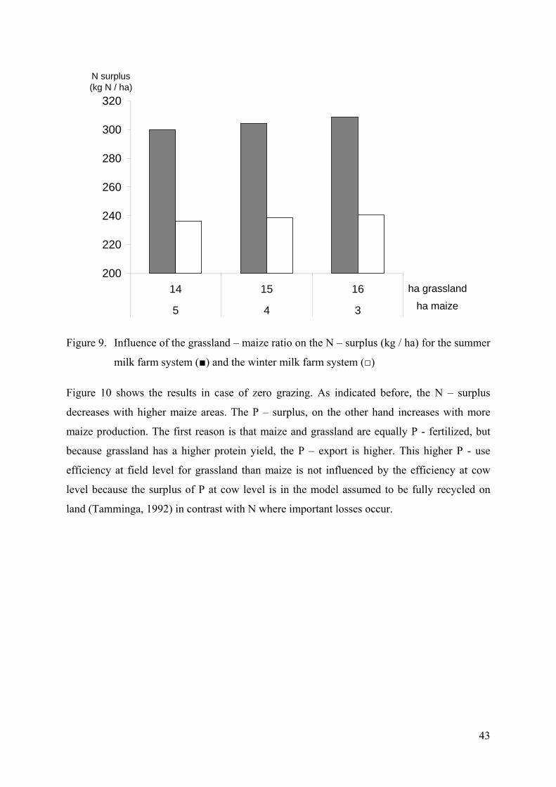
200

220

240

260

280

300

320

14 15 16

5 4 3

ha grassland

ha maize

N surplus(kg N / ha)

Figure 9. Influence of the grassland – maize ratio on the N – surplus (kg / ha) for the summer

milk farm system (■) and the winter milk farm system (□)

Figure 10 shows the results in case of zero grazing. As indicated before, the N – surplus

decreases with higher maize areas. The P – surplus, on the other hand increases with more

maize production. The first reason is that maize and grassland are equally P - fertilized, but

because grassland has a higher protein yield, the P – export is higher. This higher P - use

efficiency at field level for grassland than maize is not influenced by the efficiency at cow

level because the surplus of P at cow level is in the model assumed to be fully recycled on

land (Tamminga, 1992) in contrast with N where important losses occur.

43

0

20

40

60

80

100

120

140

160

180

17 16 15 14 13 12 11 10 9 8 7 6 5 4 3 2 1 0

0 1 2 3 4 5 6 7 8 9 10 11 12 13 14 15 16 17

Ha grassland

Ha maize

Surplus (kg/ha)

Figure 10. Influence of the grassland – maize ratio on the N – surplus (■) and P - surplus (□)

in case of zero grazing.

2.5.3 Summer milk, winter milk and zero grazing. As can be derived from Figure 11 the annual variation of N – input at cow level is influenced

by two major factors. The first and most important is the lactation curve. Two months after

calving the milk production and daily N – input reaches a maximum.

The second factor is the grazing period. Both in the winter milk farm system and summer

milk farm system a sharp increase in N – input can be observed during the grazing period.

The OEB – balance with young grass is too high, resulting in high excretion of N. The manure

produced by cows during the stable period is also better recycled than manure produced

during a grazing period. This explains the big difference in total surplus between Figure 9 and

Figure 10. It may therefore be concluded that zero grazing has a positive effect on the nutrient

balance of a dairy farm. Further, farms with grazing have higher nutrient use efficiency the

more winter milk they produce.

44

0

5

10

15

20

25

30

35

40

45

jan feb mar apr may jun jul aug sept okt nov dec

N input in kg N/day summer milk

zero grazingwinter milk

Figure 11. Annual variation of N – input for the whole herd on the summer milk, zero grazing

and the winter milk farm systems.

2.6 Sensitivity analysis

A sensitivity analysis has been performed to analyse the influence of fertilizer application

rates and the summer and winter manure coefficients on the above results and conclusions.

The simulation results in Figure 12 illustrate the positive effect of reduced N – fertilisation on

the N – surplus of a dairy farm. Figure 12 shows a similar effect for the three farm systems

modelled. This means that the level of N – fertilization does not change the conclusions of the

previous sections for the different farm systems. Zero grazing appears to be the best option for

optimal nutrient management, independent whether 200 kg N/ha or 400 kg N/ha fertilization

is used.

45

0

50

100

150

200

250

300

350

400

200 300 400kg N / ha grassland

N surplus(kg/ha)

Figure 12. N – surplus with three N – fertilization levels for the summer milk (■), winter milk

(▲) and zero grazing (□) farm systems.

For maize feeding the conclusion is different. The benefit on the N surplus of feeding maize

decreases with decreasing fertilizer levels. This can be seen by comparing the N - surplus in

Figure 10 (300 kg N/ha) and the N - surplus in Figure 13 (200 kg N/ha). For a high

fertilisation level, 100% maize gives the lowest N - surplus (Figure 10). For a lower

fertilisation level (Figure 13) the N - surplus is lower with a grass - maize mixture than with

100% maize.

46

62

64

66

68

70

72

74

76

17 16 15 14 13 12 11 10 9 8 7 6 5 4 3 2 1 0

0 1 2 3 4 5 6 7 8 9 10 11 12 13 14 15 16 17

ha grassland

ha maize

N surplus (kg/ha)

Figure 13. N – surplus for the zero grazing farm system with fertilisation of 200 kg N/ha on

grassland and 140 kg N/ha on maize.

The results of the sensitivity analysis of the summer and winter manure coefficients are

illustrated in Figure 14. The main conclusion remains valid even with very different summer

and winter manure coefficients. The N - surplus of a winter milk farm system is lower than

the surplus of a summer milk farm system even if the same manure coefficient for summer

and winter is assumed. The higher the difference between both coefficients, the higher the

difference in N - surplus in both farm systems becomes.

47

0

50

100

150

200

250

300

350

400

100 95 90 85 80 75

100 80 60 40 20 0

Winter N manure coefficient

Summer N manure coefficient

N - surplus (kg/ha)

Figure 14. N – surplus for the summer milk (▬) and the winter milk (▬) farm system with

varying summer and winter N coefficients.

2.7 Discussion

The model confirms the results of other studies (Jarvis et al., 1996, Michiels et al., 1998,

Vermeltfoort et al., 2001 ) by indicating the positive effects of supplementing grazing with

maize feeding on the N - surplus. These results have important implications for policy

measures in Flanders and The Netherlands. The Flemish and Dutch governments have asked a

derogation from the Nitrate Directive of the European Union for grassland, allowing higher

organic fertilizer applications on grassland than on other crops. This can be justified from an

agronomic viewpoint as grass is able to utilize the higher fertilisation levels more efficiently

than other crops. However, at cow level grassland is not always the best option for a low N -

surplus. A derogation for grassland could stimulate Dutch and Flemish farmers to cultivate

more grass instead of maize or other fodder crops. This would lead to an overall lower

nutrient use efficiency on the dairy farms with high fertiliser application rates. Van Bruchem

et al. (1999) report that more maize in the feed ration also results in a higher quality of the

manure produced by the cattle. As this is not simulated in the model, the positive effects of

maize could be even larger than simulated.

48

From a nutrient use efficiency perspective our model shows that zero grazing is the best

option. Vermeltfoort et al. (2001) come to a similar conclusion with a statistical comparison

of nutrient balances of different farms in the Netherlands. In practice, an increasing number of

dairy farmers (in particular in the Netherlands) already applies zero grazing.

However, besides nutrient use efficiency, also labour income is an important consequence of

management decisions. It could be expected that zero grazing results in a higher cost. With

the present model this could not be assessed (although the model contains an economic

calculation) because these costs depend too much on characteristics of the farm structure,

such as the system of milking installation and acreage of pasture near the farm, which are not

included in the model so far. Other research indicates different effects of zero grazing on

labour income. Overvest and Laeven-Kloosterman (1984) and Coléno and Duru (1999)

suggest a negative impact of zero grazing on the labour income of the farmer. On the contrary

a statistical analysis of 54 specialized dairy farms in the Netherlands showed that less grazing

has no negative impact on farm income. Bondt et al. (2001) state that farm income and

grazing are not directly linked. Larger scale farms with automated milking and limited

available land could benefit from zero grazing while smaller farms with more land could be

better off with grazing.

Van der Schans (2000) evaluates other side effects of zero grazing. He suggests a negative

impact on nature, wildlife, public perception of the dairy sector, countryside and animal

welfare. As a reaction CONO (a Dutch cheese factory) has already decided to give a price

premium of 1 eurocent per kg milk for farmers that apply grazing.

49

2.8 Conclusions

2.8.1 Conclusions with respect to the application In general, the analysis has illustrated the potential of the developed model for quantitatively

evaluating the impact of management decisions on the nutrient balance of a dairy farm. The

advantage of using models is the possibility of combining separately known functions in one

simulation in order to draw conclusions not only at field or at cow level, but also at overall

farm level. Further, external parameters influencing observed nutrient balances such as

weather conditions and measurements errors can be eliminated, so that the exact influence of

practices and systems can be evaluated. As illustrated, the model can be used to evaluate

either management options at farm level, but also the effect of possible policy options.

Introducing a number of economic and environmental indicators such as ammonia emission,

labour income, financial performance indicators and so on could extend the application range

of the model as e.g. in the models described by Herrero et al. (1999), Ramsden et al. (1999)

and van Calker et al. (2004). This will, however, require additional input parameters as well.

2.8.2 Modelling lessons The application shows that the farm-level NMP approach allows for a detailed descriptive

analysis of a dairy farm. Through the use of the list of input parameters, it is possible to

analyse different farm structures with the same model. The application indicates that NMP

models can be powerful tools for policy analysis and lead to useful policy recommendations.

The dairy farm model, and in general most farm-level NMP models, can also be used as an

advisory instrument for farmers as it can produce as, e.g., in this case a grazing and mowing

calendar or it can give more insight into the nutrient balance of the farm.

The validation of the model illustrates, however, one of the main problems of NMP, which

was also expressed by one of the reviewers of Agricultural Systems: “My main difficulty with

this paper is the model’s inability to simulate baseline conditions. This seems to result from

the use of LP to produce optimum conditions that do not prevail on farms. As a result, I do not

see how any relevance can be claimed for the intervention scenarios. “

However, the article also explains that exactly this validation problem provides us with two

important reasons to choose NMP for the development of such a detailed farm-level model.

50

First, the problems with the validation data suggest that a modelling exercise is an important

approach to separate the general impact of the chosen scenarios from external conditions

sometimes linked to farm specific conditions. Other types of assessment of the different

scenarios, such as field experiments, are largely influenced by weather, measurement errors,

and difficulties in data collection. These data difficulties do not necessarily imply that models

should not be built. It is after all better to use good logic (embodied in the model) for policy

analysis than to compound the problem of poor data with poor logic (Hazell and Norton,

1986).

Second, the validation also indicates that no data are available with enough details to calibrate

the model and turn it into a PMP or EMP model. The calibration could be performed by, e.g.,

the adjustment of manure efficiency factors. However, to do so, sufficient and accurate data

for all other parameters are needed, which are apparently not available yet. Therefore, PMP or

EMP could not be applied here.

It should, however, be noted that the model results are only meaningfull if the technology

represented in the model correspond to a common technology used by most farmers. The

main risk of an NMP model is to produce results with an assumed technology far from the

reality, which complicates interpretation and comprehension by researchers and farmers.

Another lesson from this application, which was also raised by the reviewers, is the difference

in available knowledge with respect to manure N transactions. The dairy farm model is very

detailed on the nutrient transactions from plant level to cow level and from cow level to the

product milk and the by-product manure. However, less detail is available on the

transformation of manure N to plant production. This lack of detail is due to the limited

available knowledge in literature and the wide variety of systems that could be applied. As a

consequence, the model relies on simple efficiency factors for manure.

This weakness can be attenuated in NMP models by applying a sensitivity analysis on the

efficiency factors. The sensitivity analysis can show to what extent results and conclusions

become different for different values of the efficiency factors. The sensitivity analysis is, in

general, an important instrument for NMP models.

51

2.8.3 Other experiences from the dairy farm model The dairy farm model was originally developed in Matlab and MS Excel. Because of the user

unfriendliness and the impossibility to transport the model to a computer without Matlab, it

was decided to make a standalone version of the model. The development of the standalone

version should result in three advantages:

• the model relies on only one program and should therefore easier be managed;

• the model has a GUI (Graphical User Interface) to facilitate the process of input and

management of the data, as well as the process of interpreting results;

• the model can be deployed on every PC without the need for additional software or

licenses.

Despite the advantages of a standalone model version programmed in Delphi, there are also

three important disadvantages.

The most important disadvantage is that Delphi has less mathematical features than

specialised programming languages from modelling packages such as Matlab

(http://www.mathworks.com/), GAMS (General Algebraic Modelling System:

http://www.gams.com) or AMPL (Algebraic Mathematical Programming Language:

http://www.ampl.com).

In Delphi, it is also more difficult to rely on solvers for the optimisation of a problem, while,

e.g., GAMS has a standard link with a set of more than 10 different solvers. This second

disadvantage could also be an advantage, because the optimisation algorithm could

specifically be developed for the problem in the model. However, we had not sufficient

knowledge and time to do so. Therefore, the optimisation algorithm from Brent (1973)

applied in the model is probably far less powerful than, e.g., the nonlinear solvers available in

GAMS.

The third disadvantage is that the development of a standalone version is rather time-

consuming.

52

Chapter 3 Positive Mathematical Programming: introduction to the farm-level calibrated model SEPALE

Positive mathematical programming (PMP) has renewed the interest in mathematical

modeling of agricultural and environmental policies. Before going into detail on PMP, this

chapter starts in the introduction with a short literature review of the concept ‘calibration’.

This chapter explains and discusses first the original PMP approach (Howitt, 1995a), followed

by a presentation of an individual farm-based sector model, called SEPALE. The farm-based

approach allows the introduction of differences in individual farm structures in the PMP

modeling framework. Furthermore, a farm-level model gives the possibility of identifying the

impacts according to various farm characteristics. Simulations of possible alternatives to the

implementation of the CAP Mid Term Reform illustrate the model.

Parts of this chapter have been published as:

Henry de Frahan, B., Buysse, J., Polomé, P., Fernagut, B., Harmignie, O., Lauwers, L. Van

Huylenbroeck, G., and Van Meensel, J. (2006). Positive mathematical programming for

agriculture and environmental policy analysis: review and practice. In: Weintraub, A.,

Bjorndal T., Epstein, R., and Romero, C. (Eds). Management of Natural Resources: A

Handbook of Operations Research Models, Algorithms, and Implementations. Kluwer

Academic Publishers, Kluwer´s International Series in Operations Research and Management

Science (Series Editor: Hillier, F.S.), in press.

and

53

Buysse, J., Van Huylenbroeck, G., Fernagut, B., Lauwers, L., Van Meensel, J., Baudry, A.,

Harmignie, O., Henry de Frahan, B. and Polomé, P. (2005). Impact of Alternative

Implementations of the Agenda 2000 Mid Term Review. Contributed paper presented at the

11th EAAE congress, Copenhagen, 24-27 August, 2005.

3.1 Introduction

Chapter 1 has already explained that calibration makes the difference between NMP and

PMP. Before going further into detail on PMP, we want first to shed some light on the term

‘calibration’.

Calibration is sometimes confused with the term validation, which is used in chapter 3. A

whole book could be written on the philosophical and practical issues involved in validation

(Kleijnen, 2001). In his survey, Kleijnen (2001) defines validation as determining whether the

simulation model is an acceptable representation of the real system - given the purpose of the

simulation model. Therefore, validation is more a step taken after a model has been

developed, while calibration is a step in the actual quantification of the model’s parameters.

A literature review illustrates that calibration has evolved differently in different areas of

research:

• Calibration is commonly applied to CGE models to make sure that equilibrium

conditions are satisfied (Arndt et al., 2002).

• Later calibration appears into macro-economics literature for quantification of real-

business-cycle (RBC) models and has now a wide range of applications (Hoover,

1995). In RBC models, calibration refers to the Euler equations, which is the set of

first-order conditions of a dynamic system of equations.

• In micro-economic models, calibration was widely practiced, but rarely formally

described (Howitt, 1995b). In this case, the modellers use formal or informal

calibration methods to match the model outcome to the available data base. Since the

formal description of PMP (Howitt, 1995a), calibration in sector level programming

models has become a widely applied practice. Calibration in programming models is

used to fit the parameters such that the data reflect the optimum in the model.

54

A common element in the use of calibration in the different fields of research is that empirical

data are used to quantify parameters such that the model’s outcome reflects, as close as

possible, the simulated outcome with the observed data as inputs. This model’s outcome can

be either an equilibrium (in CGE models) or an optimum of the objective function subject to

constraints (in MP models). The differences in calibration come, therefore, mainly from the

differences in data, model structure and model outcome.

Due to the wide variety of applications of calibration in economics, there is also diversity in

the definition of calibration.

Pagan (1994) calls calibration the methodology reluctant of making assumptions about error

terms because they are only treated as what is needed to reconcile the data with the model.

Kleijnen (1993) defines calibration as the adjustment of simulation model’s parameters (using

some minimisation algorithm) such that the simulated output deviates minimally from the real

output. Brown and Oman (1991) state that in calibration problems one wishes to predict a

quantity whose precise measurement is difficult or expensive to obtain by a less precise but

more easily obtained measurement.

This definition of Brown and Oman (1991) is probably true for all calibrated mathematical

programming models, since calibration would be useless if all driving factors and all

constraints of a problem were known. Calibration in the context or programming models

could therefore be considered as a simplification of the model and modelling process.

However, we prefer to use the definition of calibration in PMP provided by Hoover (1995)

and in which we replace ‘or’ by ‘and’: “A model is calibrated when its parameters are

quantified from casual empiricism or unrelated econometric studies and are chosen to

guarantee that the model precisely mimics some particular feature of the historical data.”

The definition of Kleijnen (1993) is more applicable to the type of calibration that is described

in EMP models (see Chapter 5).

55

3.2 The original PMP Approach

PMP, as formalised by Howitt (1995a), is a method to calibrate mathematical programming

models to observed behaviour during a baseline by using the information provided by the dual

variables of calibration constraints. The dual information related the vector of the observed

activity levels is used to calibrate a nonlinear objective function such that the observed

activity levels are reproduced for the baseline but without the calibration constraints. The term

"positive" that qualifies this method implies that the parameters of the non-linear objective

function are derived from an economic behaviour assumed to be rational given all the

observed and non-observed conditions that generates the observed activity levels.

PMP, as formalised by Howitt (1995a), follows a procedure in three steps. The first step

consists in writing an MP model as usual but adding to the set of limiting resource constraints

a set of calibration constraints that bound the activities to the observed levels of the baseline.

Taking the case of maximising gross margins with upper bounded calibration constraints, we

write the initial model as in Paris and Howitt (1998):

Maximise Z = p' x - c' x (26) subject to: A x ≤ b [λ] (27) x ≤ xo + ε [ρ] (28) x ≥ 0 (29)

where:

Z scalar of the objective function value, p (n x 1) vector of product prices, x (n x 1) non-negative vector of production activity levels, c (n x 1) vector of accounting costs per unit of activity, A (m x n) matrix of coefficients in resource constraints, b (m x 1) vector of available resource levels, xo (n x 1) non-negative vector of observed activity levels, ε (n x 1) vector of small positive numbers for preventing linear dependency between the

structural constraints and the calibration constraints, λ (m x 1) vector of duals associated with the allocable resource constraints, ρ (n x 1) vector of duals associated with the calibration constraints.

Assuming that all activity levels are strictly positive and all allocable resource constraints are

binding at the optimal solution, the first-order conditions of model (26) provide the following

dual values as in Heckelei and Wolff (2003):

ρp = pp - cp - Ap' λ (30) ρm = pm - cm - Am' λ = 0 (31) λ = (Am')-1 (pm - cm) (32)

56

The vector x is partitioned into [(n – m) x 1] vector of preferable activities xp constrained by

the calibration constraints (1b) and (m x 1) vector of marginal activities xm constrained by the

allocable resource constraints (1a). The other vectors ρ, p and c and the matrix A are

partitioned accordingly.

Howitt (1995a) and Paris and Howitt (1998) interpret the dual variable vector ρ associated

with the calibration constraints as capturing any type of model mis-specification, data errors,

aggregate bias, risk behaviour and price expectations. In the perspective of calibrating a non-

linear decreasing yield function as in Howitt (1995a), this dual vector ρ represents the

difference between the activity average and marginal value products. In the alternative

perspective of calibrating a non-linear increasing cost function as in Paris and Howitt (1998),

this dual vector ρ is interpreted as a differential marginal cost vector that together with the

activity accounting cost vector c reveals the actual variable marginal cost of supplying the

observed activity vector xo.

The second step of PMP consists in using these duals to calibrate the parameters of the non-

linear objective function. A usual case considers calibrating the parameters of a variable cost

function Cv that has the typical multi-output quadratic functional form, however, holding

constant variable input prices at the observed market level as follows:

Cv(x) = d' x + x' Q x / 2 (33)

where: d (n x 1) vector of parameters of the cost function, Q (n x n) symmetric, positive (semi-) definite matrix with typical element qii' for activities

i and i’.

Other functional forms are possible. The constant elasticity of substitution (CES) production

function (Howitt, 1995b) in addition to the constant elasticity of transformation production

function (Graindorge et al., 2001) have also been used.

At this point, Heckelei (2002) describes a conceptual shortcoming of PMP: the limited

rationalisation of the nonlinear terms in the model. These non-linear terms are often not

motivated by behavioural or technological assumptions but rather with determinants of supply

behaviour not captured by the other elements of the model. Heckelei (2002) describes four

different types of rationalisation of these nonlinear terms: heterogenous land quality,

unknown resource constraints, convex combination constraints to mitigate aggregation errors

or risk aversion behaviour to price uncertainty.

57

The variable marginal cost vector MCv of the typical quadratic cost function is set equal to

the sum of the accounting cost vector c and the differential marginal cost vector ρ as follows:

MCv = ∇Cv(x)xo' = d + Q xo = c + ρ (34)

where:

∇Cv(x) is a (1 x n) gradient vector of first derivatives of Cv(x) for x = xo.

To solve this system of n equations for [n + n(n + 1)/2] parameters and, thus, overcome the

under-determination of the system, PMP modellers rely on various solutions.

A first, ad hoc solution consists in assuming that the symmetric matrix Q is diagonal,

implying that the change in the actual marginal cost of activity i with respect to the level of

activity i' (i≠i') is null and, then, in relying on additional assumptions. Common additional

assumptions consist in posing the vector d of the quadratic cost function to be either equal to

zero, which leads to:

qii = (ci + ρi)/ xio and di = 0 for all i = 1, …n,

or equal to the accounting cost vector c, which leads to:

qii = ρi / xio and di = ci for all i = 1, …n.

Another calibration rule called the average cost approach equates the accounting cost vector c

to the average cost vector of the quadratic cost function, which leads to:

qii = 2 ρi / xio and di = ci - ρi for all i = 1, …n.

Exogenous supply elasticities εii are also used to derive the parameters of the quadratic cost

function as in Helming et al. (2001):

qii = pio / εii xio and di = ci + ρi - qii xio for all i = 1, …n.

All these specifications would exactly calibrate the initial model as long as equation (34) is

verified, but lead to different simulation responses to external changes.

58

A subsequent development from Paris and Howitt (1998) to calibrate the marginal cost

function is to exploit the maximum entropy estimator to determine all the [n + n(n + 1)/2]

elements of the vector d and matrix Q using the Cholesky factorisation of this matrix Q to

guarantee that the calibrated matrix Q is actually symmetric positive semi-definite.5 This

estimator in combination with PMP enables to calibrate a quadratic variable cost function

accommodating complementarity and competitiveness among activities still based on a single

observation but using a priori information on support bounds. Nevertheless, as argued in

Heckelei and Britz (2000), the simulation behaviours of the resulting calibrated model would

be still arbitrary because heavily dominated by the supports.

Heckelei and Britz (2000) exploit the suggestion from Paris and Howitt (1998) to use the

maximum entropy estimator to determine these parameters on the basis of additional

observations of the same farm or region in a view to collect information on second order

derivatives. They estimate the parameters of the vector d and matrix Q on the basis of cross

sectional vectors of marginal costs and the use of the Cholesky decomposition of the matrix of

the second order derivatives as additional constraints. They obtain a greater successful ex-post

validation than using the standard "single observation" maximum entropy approach. This

cross sectional procedure is an interesting response to the lack of empirical validation for

models that are calibrated on a single base year. The method is used to calibrate the cost

functions of the regional activity supplies of the Common Agricultural Policy Regional

Impact (CAPRI) modelling system (Heckelei and Britz, 2001).

The third step of PMP uses the calibrated non-linear objective function in a non-linear

programming problem similar to the original one except for the calibration constraints. This

calibrated non-linear model is consistent with the choice of the non-linear activity yield or

cost function derived in the preceding step and exactly reproduces observed activity levels

and original duals of the limiting resource constraints.

5 In short, the maximum entropy approach consists in estimating parameters regarded as expected values of associated

probability distributions defined over a set of a priori discrete supports (Golan et al., 1996).

59

The following PMP model is ready for simulation.

Maximise Z = p' x - d' x - x' Q x / 2 (35) subject to: A x ≤ b [λ] (36) x ≥ 0 (37)

where the vector d and matrix Q are the calibrated parameters of the non-linear objective

function.

Assuming again that i) all optimal activity levels are strictly positive and ii) allocable resource

constraints are all binding at the optimal solution and iii) Q is invertible, the first-order

conditions of model (35) provide the following dual values of the resource constraints as in

Heckelei and Wolff (2003):

λ = (A Q -1 A') -1 (A Q -1 (p - d) - b) (38)

This calibration approach has been applied at the farm, regional and sector levels. When

accounting data of a sample of F farms are available such as from the FADN, F PMP models

can be defined for each farm of the sample. Simulations can then be performed on these

individual PMP models and simulation results may be aggregated as shown in the application

in section 3.5. The fact that this is possible increases the farm level information that such

models can yield as will be shown in Chapter 5.

3.3 Discussion of the original PMP Approach

Section 1.3 explains that the basic idea behind the calibration of a programming model is to

assign all unknown parameter in such a way that the optimality conditions are satisfied for the

empirical data. In most cases, the modeller has not sufficient data and has to rely on

assumptions and/or simplifications.

60

In the original PMP approach (Howitt, 1995a) the assumptions that have to be made are

divided in the first two steps of the PMP. The first step of the original PMP approach makes

an assumption by assigning the highest possible values to the dual of the resource constraint6.

The value of ε in equation (28) plays an important role in this assumption. Howitt (1995a)

explains that this small number is used to decouple the structural constraints from the

calibration constraints. However, depending on the scaling of the original problem different

values of ε can return different duals of calibration constraints. Paris (2001) state that if the

dual of the resource constraints become zero, ε is too low.

The second step of making assumptions solves the under-determination problem in equation

(34). As explained above, PMP modellers rely therefore on various solutions. Some of these

solutions try to reduce the use of restrictive assumptions to a minimum by exploiting multiple

observations and estimation techniques (Heckelei and Britz, 2001). However, these

estimations start with the assumptions made in the first step of PMP and are therefore likely

biased.

For that reason, Heckelei and Wolff (2003) recently explain that the original PMP approach is

not well suited to the estimation of programming models that use multiple cross-sectional or

chronological observations. They show that the derived marginal cost conditions (8) prevent a

consistent estimation of the parameters when the ultimate model (7) is seen as representing

adequately the true data generating process. Their argument goes as follows. On the one hand,

the shadow price value vector λ implied by the ultimate model (7) is determined by the

vectors p, d and b and the matrices A and Q through the first-order condition derived

expression (8). On the other hand, the various dual value vectors λ from the sample initial

6 The dual value of the resource constraints of phase 1 of original PMP is the highest possible if it is assumed that the total

cost correspond to the sum of the observed accounting costs used in phase 1 of PMP and some potential unobserved costs.

These observed accounting cost define then a minimum for the calibrated total cost function.

Equation (31) and (32) illustrate that the PMP model would then be calibrated for any value of the dual of the resource

constraint in the interval [0 - λ]. However, if the value of the dual of the resource constraint would be λ + e (e is a very small

positive number), the dual of the calibration constraint of the marginal crop would become negative:

ρm = pm - cm - Am' [(Am')-1 (pm - cm) + e] = - Am' e

This negative dual for the calibration constraint implies that the model would not be perfectly calibrated anymore because the

simulated quantities for the marginal crop would be lower than the observed quantities.

61

model are solely determined by the vectors p and c and matrix A of only those marginal

activities bounded by the resource constraints through the first-order derived expression (4).

As a result, the various vectors λ of resource duals of the initial models are most generally

different from the vector λ of resource duals of the ultimate model. Since the first step

simultaneously sets both the initial dual vectors ρ and λ and the second step uses the initial

dual vector ρ to estimate the vector MCv, this latter vector must generally be inconsistent with

the ultimate model. The derived marginal conditions are, therefore, most likely to be biased

estimating equations yielding inconsistent parameter estimates.7

To avoid inconsistency between steps 1 and 3 as further exposed in Heckelei and Britz

(2005), Heckelei and Wolff (2003) suggest to skip the first step altogether and employ

directly the optimality conditions of the desired programming model to estimate and calibrate

simultaneously shadow prices and parameters. They illustrate this general alternative to the

original PMP through three examples relying on the Generalised Maximum Entropy (GME)

procedure for estimating the model parameters. Their examples deal with the estimation of the

parameters of various optimisation models that (1) incorporate a quadratic cost function and

only one constraint on land availability, (2) allocate variable and fixed inputs to production

activities represented by activity-specific production functions or (3) allocate fixed inputs to

production activities represented by activity-specific profit functions.

3.4 Further PMP developments

While being an appealing method for calibration, PMP has shown shortcomings in model

calibration that, in turn, motivated further developments. One of these shortcomings is the

missing representation of economic behaviours with regard to activities of farms whose initial

observed supply level is zero during the baseline. To overcome this self-selection problem

during the calibration as well as during the simulation steps, Paris and Arfini (2000) add to the

F PMP models a supplementary PMP model for the whole farm sample and calibrate a

frontier cost function for all the activities included in the whole farm sample.

A second development of the PMP methodology concerns the integration of risk. For

example, Paris (1997) uses a von Neumann-Morgenstern expected utility approach assuming

a normal distribution of output prices and a constant absolute risk aversion.

7 In other words, the ‘estimated’ value of the dual vector λ cannot converge to the true dual vector λ as more observations are

added because PMP always selects the highest possible value for the dual vector λ.

62

A third development is the inclusion of greater competitiveness among close competitive

activities whose requirements for limiting resources are more similar than with other

activities. Rohm and Dabbert (2003) represent these close competitive activities as variant

activities from their generic activities and add to the first PMP step calibration constraints for

these variant activities that are less restrictive than their counterparts for their generic

activities.

A fourth development to overcome criticisms that have been raised against the use of a linear

technology in limiting resources and the zero-marginal product for one of the calibrating

constraints is the expansion of the PMP framework into a Symmetric Positive Equilibrium

Problem (SPEP). Paris (2001) and Paris and Howitt (2001) express the first step of this new

structure as an equilibrium problem consisting of symmetric primal and dual constraints and

the third step as an equilibrium problem between demand and supply functions of inputs, on

the one hand, and between marginal cost and marginal revenue of the output activities, on the

other hand. For these authors, the key novelty of this new framework is rendering the

availability of limiting inputs responsive to output levels and input price changes. Britz et al.

(2003), however, address several conceptual concerns with respect to the SPEP methodology

and question the economic interpretation of the final model ready for simulations.

3.5 SEPALE: System for evaluation of agro- and agro-environmental policies.

This section illustrates how the PMP concept can be applied within an agricultural model that

can be used to simulate various policy scenarios. The agricultural model is composed of a

collection of micro-economic mathematical programming models each representing the

optimising farmer's behaviour at the farm level. Parameters of each PMP model are calibrated

on decision data observed during a baseline exploiting the optimality first-order conditions

and the observed opportunity cost of limiting resources. Simulation results can be aggregated

according to farm localisation, type and size.

63

Exploiting the richness of the FADN data, this model is part of an effort initially funded by

the Belgian Federal Ministry of Agriculture to develop a decision support system for

agricultural and environmental policy analysis. The model is known under the name of

SEPALE and is developed by a group of agricultural economists based at the Université

Catholique de Louvain, the University of Ghent and the Centre for Agricultural Economics of

the Ministry of the Flemish Community. Since this model predominantly uses FADN data, it

is conceivably applicable to all the EU-15 58000 representative commercial farms recorded in

this database accessible by any national or regional administrative agencies.

Before presenting an application drawn from the June 2003 CAP reform (also called mid-term

review of Agenda 2000), the following subsection first presents how key parameters of the

model are calibrated in the farm generic model and how animal feeding and quota constraints

are added to the generic farm model.

3.5.1 Description of the basic farm model The model consists of a compilation of individual farm mathematical programming (MP)

models following the general calibration approach described in the previous chapters. We

derive directly, as also Judez et al. (2001) suggest, the unknown parameters of the final non-

linear model from the Kuhn-Tucker conditions of such final model considering exclusively

the activities whose observed levels are different from zero and the opportunity costs of the

limiting resources as given exogenously to the model.

On the premise that farms are able to acquire farmland from other farms, farmland is here

supposed to be not a binding resource at the farm level, merely an expensive one, and enter

into the variable cost component.8

The individual farm model relies on a farm level profit function using the typical simplified

quadratic functional form for its cost component. In matrix notation, this gives:

Zf = pf' xf + af' Sf xf - xf' Qf xf / 2 - df' xf (39)

with

f indexing the farms from 1 to F,

8 The reader may verify from model (1) that the quadratic parameter matrix Q is invariant to whether keeping the

binding constraint on farmland and using the farmland rental cost as a proxy for its shadow value or removing

the farmland binding constraint and including the farmland rental cost in the average cost. The linear vector d is

just inflated by the value of the farmland rental cost in the latter alternative.

64

where:

xf is a (N x 1) column vector of production quantities (indexed by i),

pf is a (N x 1) column vector of output prices per unit of production quantity (indexed

by i),

af is a (N x 1) column vector of technical coefficients determining how much resource

base (i.e., farmland) is needed per unit of production quantity xif,

Sf is a (N x N) diagonal matrix of subsidies per unit of resource base,

Qf is a (N x N) diagonal matrix of quadratic cost function parameters,

df is a (N x 1) vector of linear cost function parameters (indexed by i).

Two sets of equations calibrate the parameters of the matrix Qf and the vector df, relying on

the technical coefficients afo, output quantities xfo, output prices pfo, subsidies Sfo and unit

production costs cfo observed at the baseline.

The first-order conditions of model (39) determine the first set of equations for strictly

positive production quantities xfo as follows:

pfo + Sfo afo = Qf xfo + df (40)

The second set of equations equates the observed average costs cfo to the average costs

implied by model (39) as follows:

cfo = Qf xfo/2 + df (41)

with cfo the (N x 1) column vector of observed costs per unit of production quantity that

include costs of seeds, fertilizers, pesticides, contract work and other costs as well as farmland

rental cost gathered from the FADN for each farm f.

The following two sets of equations calibrate the diagonal matrix Qf and the vector df for each

farm f of the sample as follows:

Qf = 2 (i xfo')-1 i (pfo + Sfo afo - cfo )' (42)

df = 2 cfo - pfo - Sfo' afo (43)

where:

i is a (N X 1) unit column vector.

With these parameters, the farm model (39) is exactly calibrated to the baseline and is ready

for simulation. Simulations simultaneously run the compilation of the F calibrated farm

models with the following additional land constraint over the F farms:

f

F

f 1

a 'x=∑ f = (44) f fo

F

f 1

a 'x=∑

65

As a consequence of the overall land constraint, land is freely exchanged across farms during

simulations and allocated to farms that use it most profitably. The model does not distinct

between buying and renting for exchanging of land use. The dual of the overall land

constraint indicates variations in the land opportunity cost with respect to its initial cost. This

dual is zero for the baseline because the cost of land is included in the cost function.

Afterwards, individual farm simulation results can be aggregated according to farm

localisation, type and size.

The basic model is further extended with feeding and quota constraints. The feeding

constraint uses a CES function that allows substitution between on-farm forage crops and off-

farm feed that is calibrated on feedings observed at the baseline. The A and B sugar quota

constraint is included into the first-order conditions of model (15) by adding to the right side

of equation (16) the dual of the sugar beet quota. The gross margin differential between the A

and B sugar beets and the next best alternative crop that is observed at the baseline

approximates this dual. As explained in Buysse et al. (2004), the supply of A and B sugar

beets includes a precautionary C supply and a quota exchange mechanism allows for a quota

redistribution among sugar beet farms within the sample. Chapter 4 and Chapter 5 provide

more details on the precautionary supply function and the quota exchange.

3.5.2 Simulation of the Mid-term Review of Agenda 2000 To illustrate the model, we apply it to assess the effects of the June 2003 CAP reform for a

sample of Belgian farms. The three main elements in the Mid-Term Review (MTR) of

Agenda 2000 are direct payment decoupling, cross-compliance and modulation. First, the

decoupling of direct payments implies that one single farm payment replaces the previous

direct payments that were linked to activities. Second, the cross-compliance renders the single

farm payment subject to farm compliance with rules related to food safety, animal health and

welfare and good agricultural and environmental practices. Third, the modulation introduces a

system of a 5% progressive reduction of the direct payments that are higher than a threshold

of 5 000 euro per farm9. The following subsections show how the basic model is modified to

incorporate the provisions of the new MTR policy instruments.

9 The savings on these direct payments are added to the financing of the rural development measures defined into

the CAP. Within the transitory options offered by the MTR, the Belgian government chooses to decouple all

direct payments except payments for suckler cows and veal slaughters.

66

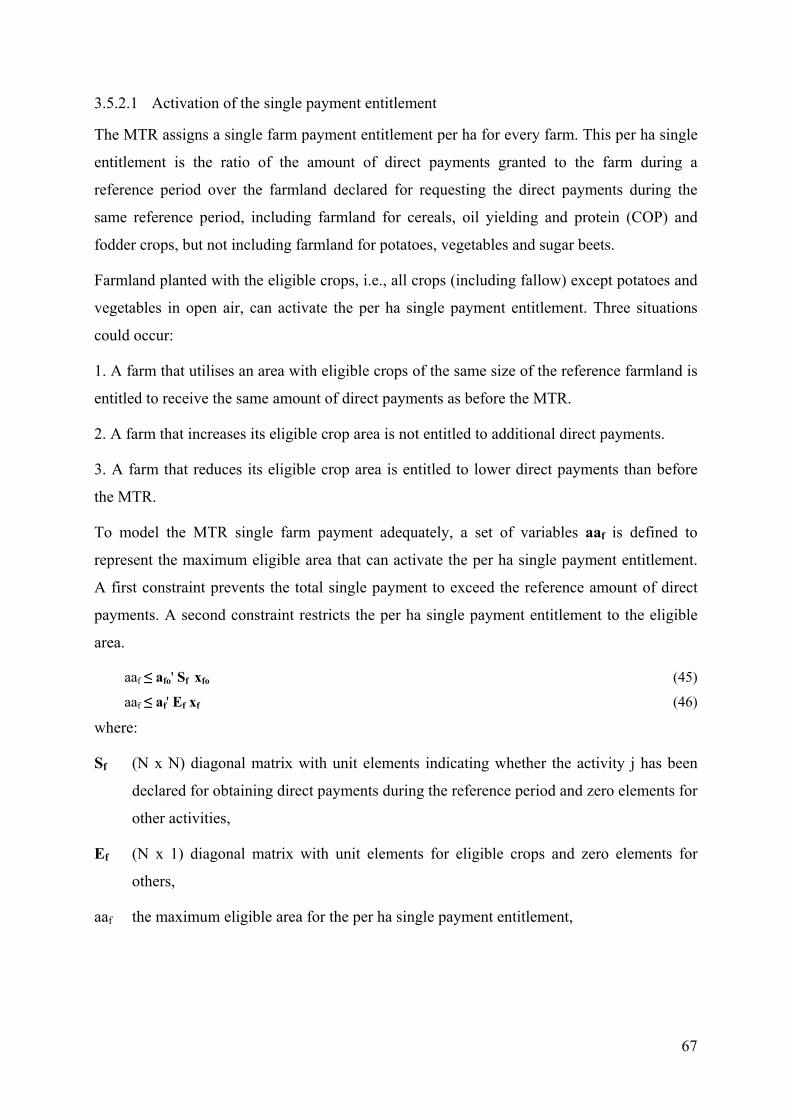
3.5.2.1 Activation of the single payment entitlement

The MTR assigns a single farm payment entitlement per ha for every farm. This per ha single

entitlement is the ratio of the amount of direct payments granted to the farm during a

reference period over the farmland declared for requesting the direct payments during the

same reference period, including farmland for cereals, oil yielding and protein (COP) and

fodder crops, but not including farmland for potatoes, vegetables and sugar beets.

Farmland planted with the eligible crops, i.e., all crops (including fallow) except potatoes and

vegetables in open air, can activate the per ha single payment entitlement. Three situations

could occur:

1. A farm that utilises an area with eligible crops of the same size of the reference farmland is

entitled to receive the same amount of direct payments as before the MTR.

2. A farm that increases its eligible crop area is not entitled to additional direct payments.

3. A farm that reduces its eligible crop area is entitled to lower direct payments than before

the MTR.

To model the MTR single farm payment adequately, a set of variables aaf is defined to

represent the maximum eligible area that can activate the per ha single payment entitlement.

A first constraint prevents the total single payment to exceed the reference amount of direct

payments. A second constraint restricts the per ha single payment entitlement to the eligible

area.

aaf ≤ afo' Sf xfo (45)

aaf ≤ af' Ef xf (46)

where:

Sf (N x N) diagonal matrix with unit elements indicating whether the activity j has been

declared for obtaining direct payments during the reference period and zero elements for

other activities,

Ef (N x 1) diagonal matrix with unit elements for eligible crops and zero elements for

others,

aaf the maximum eligible area for the per ha single payment entitlement,

67

The direct payments extend the profit function, as follows:

Zf = pf' xf + aaf afo' Subsfo Df xfo (afo' xfo)-1 + af' Subsfo (I - Df) xf

- xf' Qf xf /2 - df' xf (47)

where:

Df (N x N) diagonal matrix with the production decoupling ratio of activity i,

I (N x N) unit matrix.

3.5.2.2 Modulation of direct payments

Modulation reduces all direct, coupled and non-coupled, payments, beyond 5 000 euro per

farm by a maximum of 5% in 2007. Modulation can, however, be avoided by transfers of

direct payment entitlements. Farms with direct payments higher than the threshold of 5000

euro can transfer their direct payment entitlements to farms with direct payments lower than

the threshold of 5 000 euro. To simulate these transfers that could be induced by modulation,

the amount of reduced direct payments should be calculated during the optimisation process

of the model to take modulation into account correctly. Therefore, the following constraint is

introduced into the model:

md ≥ afo' Subsfo Df xfo (afo' xfo)-1 + af' Subsfo (I - Df) xf - mt (48)

where:

md the positive amount of direct payments subject to modulation,

mt the amount of direct payments free from modulation.

Modulation extends the profit function as follows:

Zf = pf' xf + aaf afo' Subsfo Df xfo (afo' xfo)-1 + af' Subsfo (I - Df) xf

- xf' Qf xf /2 - df' xf - md mp (49)

where:

mp the modulation percentage.

Although the MTR modulation imposes an increase in the modulation percentage in three

steps from 3% in the first year, 4 % in the second year and 5% in the third, the following

analysis is restricted to the simulation of the final modulation percentage.

68

3.5.2.3 Transfers of direct payment entitlements

Transfers of direct payments entitlements can occur both with and without transfer of land. A

certain percentage of the entitlements that are transferred can, however, be withhold by the

member state. For entitlement transfers with land, 10% of the entitlement can revert to the

national reserve while, for sole transfers of direct payment entitlements, up to 30% of the

entitlement can revert to national reserve. Seven additional constraints and seven additional

variables are used to model the transfers of direct payment entitlements leaving open the

possibility to realise these transfers with and without land transfers. Unobserved transaction

costs can play a major role in the decision to transfer direct payment entitlements but are not

modelled here.

First, a constraint determines per farm the amount of not activated direct payments

entitlements, as follows:

naf = afo’ xfo Sf - aaf (50)

where

naf: not activated direct payment entitlements (in ha)

Then, following constraint calculates the average amount of direct payments per ha of not

activated entitlements:

avs = ∑f ( naf afo’ Subsfo xfo Df * (afo’ xfo)-1 ) / ∑f naf (51)

where

avs: the average amount of direct payments per ha of not activated entitlements

Farms with eligible land not yet used for activating decoupled direct payments will induce the

direct payment entitlement transfers, because they are interested in buying entitlements.

Following constraint calculates the free eligible land on each farm:

eff = af’ xf Ef - aaf (52)

eff : free eligible land

69

The farms with free eligible land can obtain additional entitlements both with as without land

transfers. To distinguish between activated direct payments with land transfer and without

land transfer, a constraint calculates the amount of land acquired by the farm, as following:

wlf ≤ absolute value(af’ xf - afo’ xfo) (53)

where

wlf ≥ 0

wlf: land used for activating transferred direct payments with land transfer

In addition, a constraint limits the sum of activated direct payments of both with and without

land transfer to be smaller than the free eligible land:

eff ≥ wlf + olf (54)

where

olf: land used for activating transferred direct payments without land transfer

The sum of not activated direct payment entitlements should always be larger than the sum of

transferred direct payments, expressed by following constraint:

∑f naf ≥ ∑f wlf + olf (55)

The dual of equation (55) gives an indication of the price of the direct payment entitlements.

A zero dual indicates that there is more supply than demand for the entitlements. The price

will then be low. The higher the dual the more demand and the higher the price of the

entitlements will be.

70

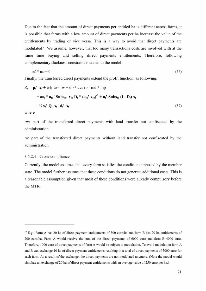
Due to the fact that the amount of direct payments per entitled ha is different across farms, it

is possible that farms with a low amount of direct payments per ha increase the value of the

entitlements by trading or vice versa. This is a way to avoid that direct payments are

modulated10. We assume, however, that too many transactions costs are involved with at the

same time buying and selling direct payments entitlements. Therefore, following

complementary slackness constraint is added to the model:

eff * naf = 0 (56)

Finally, the transferred direct payments extend the profit function, as following:

Zn = pf’ xf + wlf avs rw + olf * avs ro - md * mp

+ aaf * afo’ Subsfo xfo Df * (afo’ xfo)-1 + af’ Subsfo (I - Df) xf

- ½ xf’ Qf xf - df’ xf (57)

where

rw: part of the transferred direct payments with land transfer not confiscated by the

administration

ro: part of the transferred direct payments without land transfer not confiscated by the

administration

3.5.2.4 Cross-compliance

Currently, the model assumes that every farm satisfies the conditions imposed by the member

state. The model further assumes that these conditions do not generate additional costs. This is

a reasonable assumption given that most of these conditions were already compulsory before

the MTR.

10 E.g.: Farm A has 20 ha of direct payment entitlements of 300 euro/ha and farm B has 20 ha entitlements of

200 euro/ha. Farm A would receive the sum of the direct payments of 6000 euro and farm B 4000 euro.

Therefore, 1000 euro of direct payments of farm A would be subject to modulation. To avoid modulation farm A

and B can exchange 10 ha of direct payment entitlements resulting in a total of direct payments of 5000 euro for

each farm. As a result of the exchange, the direct payments are not modulated anymore. (Note the model would

simulate an exchange of 20 ha of direct payment entitlements with an average value of 250 euro per ha.)

71

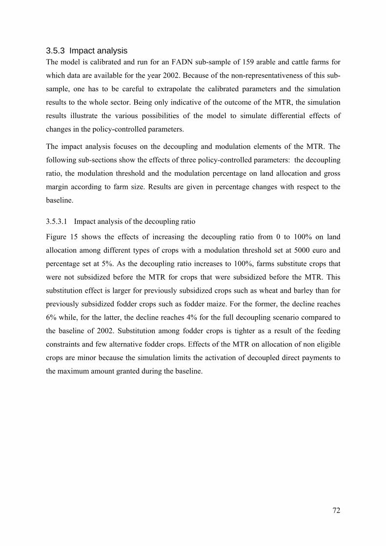
3.5.3 Impact analysis The model is calibrated and run for an FADN sub-sample of 159 arable and cattle farms for

which data are available for the year 2002. Because of the non-representativeness of this sub-

sample, one has to be careful to extrapolate the calibrated parameters and the simulation

results to the whole sector. Being only indicative of the outcome of the MTR, the simulation

results illustrate the various possibilities of the model to simulate differential effects of

changes in the policy-controlled parameters.

The impact analysis focuses on the decoupling and modulation elements of the MTR. The

following sub-sections show the effects of three policy-controlled parameters: the decoupling

ratio, the modulation threshold and the modulation percentage on land allocation and gross

margin according to farm size. Results are given in percentage changes with respect to the

baseline.

3.5.3.1 Impact analysis of the decoupling ratio

Figure 15 shows the effects of increasing the decoupling ratio from 0 to 100% on land

allocation among different types of crops with a modulation threshold set at 5000 euro and

percentage set at 5%. As the decoupling ratio increases to 100%, farms substitute crops that

were not subsidized before the MTR for crops that were subsidized before the MTR. This

substitution effect is larger for previously subsidized crops such as wheat and barley than for

previously subsidized fodder crops such as fodder maize. For the former, the decline reaches

6% while, for the latter, the decline reaches 4% for the full decoupling scenario compared to

the baseline of 2002. Substitution among fodder crops is tighter as a result of the feeding

constraints and few alternative fodder crops. Effects of the MTR on allocation of non eligible

crops are minor because the simulation limits the activation of decoupled direct payments to

the maximum amount granted during the baseline.

72

-8

-6

-4

-2

0

2

4

6

0 25 50 75 100 decoupling ratio

change in land use (%)

nonsubsidizedcrops

nonsubsidizedfodder crops

non eligiblecrops

subsidizedfodder crops

subsidizedcrops

Figure 15. Changes in land allocation among crop categories with respect to the decoupling

ration

Figure 16 shows the effects of increasing the decoupling ratio from 0 to 100% on farm gross

margins across farm sizes with a modulation threshold set at 5000 euro and percentage set at

5%. Effects of the MTR on farm gross margins are relative smaller than effects on land

allocation. As expected, a complete decoupling of the direct payments generates a positive

effect on farm gross margins across all farm sizes. The larger positive effect in gross margin

for farms of smaller size is due to the 5% modulation of direct payments above the threshold

of 5000 euro.

73

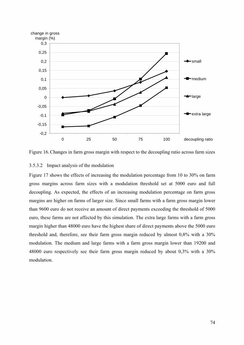
-0,2

-0,15

-0,1

-0,05

0

0,05

0,1

0,15

0,2

0,25

0,3

0 25 50 75 100 decoupling ratio

change in gross margin (%)

small

medium

large

extra large

Figure 16. Changes in farm gross margin with respect to the decoupling ratio across farm sizes

3.5.3.2 Impact analysis of the modulation

Figure 17 shows the effects of increasing the modulation percentage from 10 to 30% on farm

gross margins across farm sizes with a modulation threshold set at 5000 euro and full

decoupling. As expected, the effects of an increasing modulation percentage on farm gross

margins are higher on farms of larger size. Since small farms with a farm gross margin lower

than 9600 euro do not receive an amount of direct payments exceeding the threshold of 5000

euro, these farms are not affected by this simulation. The extra large farms with a farm gross

margin higher than 48000 euro have the highest share of direct payments above the 5000 euro

threshold and, therefore, see their farm gross margin reduced by almost 0,8% with a 30%

modulation. The medium and large farms with a farm gross margin lower than 19200 and

48000 euro respectively see their farm gross margin reduced by about 0,3% with a 30%

modulation.

74

-0,9

-0,8

-0,7

-0,6

-0,5

-0,4

-0,3

-0,2

-0,1

0

0,1

0,2

10 15 20 25 30 modulation percent


Small

Medium

Large

Extra Large

Figure 17. Changes in farm gross margin with respect to the modulation percentage across

farm sizes

Figure 18 shows the effects of decreasing the modulation threshold from 5 000 to 2 000 euro

on farm gross margins across farm sizes with a modulation percentage set at 5% and full

decoupling. As expected, a lower modulation threshold leads to a decline in farm gross

margin across all farm sizes. This decline is larger for farms of smaller size. A reduction of

the modulation threshold combined with an increase in the modulation percentage results in

even larger decline in farm gross margins.

75

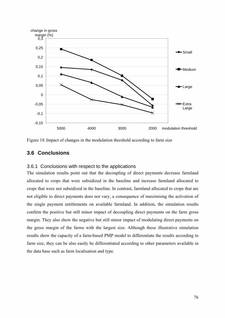
-0,15

-0,1

-0,05

0

0,05

0,1

0,15

0,2

0,25

0,3

5000 4000 3000 2000 modulation threshold


Small

Medium

Large

ExtraLarge

Figure 18. Impact of changes in the modulation threshold according to farm size

3.6 Conclusions

3.6.1 Conclusions with respect to the applications The simulation results point out that the decoupling of direct payments decrease farmland

allocated to crops that were subsidized in the baseline and increase farmland allocated to

crops that were not subsidized in the baseline. In contrast, farmland allocated to crops that are

not eligible to direct payments does not vary, a consequence of maximising the activation of

the single payment entitlements on available farmland. In addition, the simulation results

confirm the positive but still minor impact of decoupling direct payments on the farm gross

margin. They also show the negative but still minor impact of modulating direct payments on

the gross margin of the farms with the largest size. Although these illustrative simulation

results show the capacity of a farm-based PMP model to differentiate the results according to

farm size, they can be also easily be differentiated according to other parameters available in

the data base such as farm localisation and type.

76

3.6.2 Modelling lessons The experience from the SEPALE exercise with respect to future modelling challenges is

discussed in the three next subsections. First, the advantages of PMP in SEPALE are listed.

Next, the limitation of the functional form, which is inherent to the application of PMP in

SEPALE, is discussed. The chapter finishes with some specific encountered problems in this

application.

3.6.2.1 PMP advantages

PMP has renewed the interest in mathematical modelling for agricultural and environmental

policies for several reasons. The main advantages of the PMP approach are the simplicity of

the modelling of bio-economic constraints or policy instruments and the possibility to make

use of very few data to model agricultural policies, while being able to generate plausible

results. The plausibility of the results is obtained from the possibility of the introduction or

real-world constraints and of the calibration step. The calibration avoids the critique of one of

the reviewers on Chapter 2: “the model’s inability to simulate baseline conditions, resulting

form optimum conditions that do not prevail on farms.”

The SEPALE application also illustrates how PMP can be used with large farm-level samples.

This not only makes it possible to account for the individual farm structure, but also for the

direct payment entitlement trade mechanisms. The results prove the relevance of the model

for simulating possible alternatives to the implementation of the CAP Mid Term Review, but

this example is certainly not limitative. The possibility of distinguishing the effects according

to farm size or other criteria such as region or farm type is one of the main advantages of the

individual farm-base modelling. It also opens avenues to model structural changes of the

sector.

3.6.2.2 PMP limitations

The plausible results generated by a PMP model do, however, not guarantee that the response

is correct. At this stage, some words of caution need to be addressed on the model

specification, which determines the model response, and should be reminded for the

interpretation of the simulation results.

77

First, the simplicity of the quadratic cost function for parameter calibration is obtained by

suppressing all input prices and off-diagonal elements from the cost function. This simplicity

implies that we can not simulate explicitly changes in yields as consequence of changed input

use such as fertilizer, seed or pesticides at the farm level. It is, however, possible to see

changes in input use due to the changed output mix and shifts of the land use between farms.

The quadratic form of the cost function also imposes marginal cost functions that are linear

and increasing with production quantities.

Second, while avoiding aggregation errors, the definition of a cost function at the farm level is

prone to a self-selection problem due to the missing representation of the farm behaviour with

respect to activities not observed during the baseline.

Third, constraining farmland over the F farms in the sample, which allows for competition

and transaction of farmland among farms gives to the model a source of jointness at the

aggregate level. This source of jointness among activities at the aggregate level as well as the

linearity of the increasing cost function provide a long-term perspective to the rate of farm

adjustment to changing economic conditions that is, however, mitigated by the fixed input

proportionality and activity selection assumptions. For example, in simulation runs, farms can

trade land to each other in the sample and re-allocate it among their baseline activities but

cannot substitute one input for another and initiate new activities.

The shortcomings raised from the use of a simplified quadratic cost function point out the use

of a flexible multi-input multi-output cost function and panel data to estimate its numerous

parameters. The shortcoming from the self-selection problem is difficult to overcome without

ad hoc modelling decisions.

The problems of assessing correctly the response behaviour are illustrated by the few ex post

simulation exercises that have been done.

78

Heckelei and Britz (2000) compare the percentage national deviation of simulated production

activity levels from the observed activity levels in 1994 for three approaches. The original

PMP approach (Howitt, 1995a), an intelligent no-change scenario and their approach that

combines PMP with Maximum Entropy (ME) are put side by side. The original PMP

approach shows rather high deviations for some major crops, while the intelligent no-change

forecast is comparatively close to observed production activity levels. The 1992 CAP-reform

had, apparently, in France a relatively small impact on the aggregate crop rotation apart from

the set-aside. The fit of the ME-PMP approach based on the cross sectional sample is rather

promising, because it provides in most cases better simulated values than the no-change

results.

Gocht (2005) compares the simulation behaviour of different PMP approaches and concludes

that all approaches which uses the first step of the Howitt (1995a) approach show large

percentage absolute deviations. The use of ME or exogenous supply elasticities has barely

improved the results.

Arriaza and Gomez-Limon (2003) perform a comparative study that besides PMP also

includes NMP models. This paper indicates that two modelling approaches that include

expected total gross margin and a qualitative total risk index outperforms other modelling

alternatives. These approaches yield the best results in terms of predictive capacity to the

1992 EU agricultural policy reform. Although the PMP approach performs well, it has the

limitation of excluding crops that are not present in the base year. However, if the excluded

crops are not regarded as a real alternative for the farmer, this approach yields satisfactory

predictions. Arriaza and Gomez-Limon (2003), however, indicate that all the conclusions

obtained are completely dependent of the context situation and, therefore, of the particular

case study. This remark is of course valid for the other validation exercises too.

3.6.2.3 Numerical solution problems

Another important but often not in detail described problem of operational modeling is

optimizing the developed simulation model. Currently, GAMS with the CONOPT3 solver

optimizes the proposed model. Three problems arise during optimization, the use of the

absolute value function (ABS), the discontinuities in the model and the complementary

slackness constraints. Due to the size of the model, i.e. the large number of variables and

constraints, solving the optimization problems remains the most difficult task in current

analysis.

79

The ABS function

The use of the ABS function in GAMS requires that the model runs as a dynamic non linear

programming (DNLP) model instead of a non linear programming (NLP) model. The NLP

solvers used by GAMS can also be applied to DNLP models. However, it is important to

know that the NLP solvers attempt to solve the DNLP model as if it was an NLP model

(Drud, 2004).

Therefore, Drud (2004) suggest two approaches to rewrite the ABS function in a NLP model.

In the first approach, the term z = ABS(f(x)) is replaced by z = fplus + fminus, fplus and

fminus are declared as positive variables and they are defined with the identity: f(x) =E= fplus

- fminus. The discontinuous derivative from the ABS function has disappeared and the part of

the model shown here is smooth. The discontinuity has been converted into lower bounds on

the new variables, but bounds are handled routinely by any NLP solver. The feasible space is

larger than before (Drud, 2004).

The second approach relies on a smooth approximation. A smooth GAMS approximation for

ABS(f(x)) is SQRT( SQR(f(x)) + SQR(delta) ) where delta is a small scalar. The value of

delta can be used to control the accuracy of the approximation and the curvature around f(x) =

0.

The approximation shown above has its largest error when f(x) = 0 and smaller errors when

f(x) is far from zero. If it is important to get accurate values of ABS exactly when f(x) = 0,

then Drud (2004) suggest following smooth approximation:

SQRT( SQR(f(x)) + SQR(delta) ) - delta

The presented model has employed both the smooth as the non-smooth reformulation of the

DNLP to the NLP model. In contrast to what Drud (2004) suggest, the value of the objective

function shows that in current model the DNLP formulation is in all simulations better than

the reformulations to NLP.

Complementary slackness constraints

A complementary slackness constraint prevents farms to buy and to sell direct payments

entitlements at the same time.

eff * naf = 0

80

However, the use of so-called complementary slackness constraints is a problem in any NLP

model (Drud, 2004). The feasible space consists of the two half lines: (eff = 0 and naf ≥ 0 )

and (eff ≥ 0 and naf = 0). Unfortunately, the marginal change methods used by most NLP

solvers cannot move from one half line to the other, and the solution is stuck at the half line it

happens to reach first (Drud, 2004). One way to solve the complementary slackness constraint

problem in current models is the use of different starting points. The objective value of the

different simulations should then determine the final retained solution. The problem here is

that a good starting point for one farm can be a bad starting point for another.

Discontinuities in the model

The solver stops each simulation run with following message.

The message indicates that there is no progress at all in the solution process. However, the

optimality criteria have not been satisfied. This problem with the presented model is caused

by discontinuities. A complex nonlinear model may — and frequently will — have multiple

locally optimal solutions. In most realistic cases, the number of such local solutions is

unknown, and the quality of local and global solutions may differ substantially. Therefore

multi-extremal decision models can be very difficult, and — as a rule — standard

optimization strategies are not directly applicable to solve them (Pinter, 2001). Here too,

global optimization could be a solution to the problem. We have tried Global Optimization

(GO) solvers, but unfortunately, they did not succeed to solve the problem. One of the GO

doesn’t even accept problems with the size of our model.

3.6.2.4 Chosen solution

At this moment, no satisfying solution has been found. The main path for improvement can be

expected from the translation from the model to an MPEC (Mathematical Programming with

Equilibrium Constraints) model and the use of the MPEC solver in GAMS. This solver is,

however, only in beta status and gives also no guarantee for success.

Due to the problems of the simulation of the transactions of direct payment entitlements,

following applications only include the equations to calculate the decoupled payment and

modulation without the possibility of transfers.

81

This simplification implies that during simulation no transfers of direct payment entitlements

occur. A farm that does not activate the entitlements, therefore, does not receive the direct

payments and other farms can not buy and, thus, not benefit from the free direct payment

entitlements. As a result, farms in the following simulations try to activate as much as

possible the entitlements. This reflects a situation with very high transaction costs for the

transactions.

82

Chapter 4 PMP extension of SEPALE: modelling the impact of policy reforms on Belgian sugar beet suppliers

Chapter 4 extends the basic farm model SEPALE, described in previous section, with a

module to deal with quota, an instrument that is often applied in European agricultural

policies.

Quotas enable policy makers to internalise national resource constraints at farm level. Quota

or production permits exist in both agricultural policies, such as the CAP (Common

Agricultural Policy), as in environmental policies. Examples of production quota in

agricultural policies are the quota for milk, suckler cows, sheep and sugar beet. Supply within

quota limits ensures suppliers a high guaranteed price for milk and sugar or subsidies for

sheep and suckler cows. These quotas allow for better control of the total budget for price or

subsidy support, which is here the national resource constraint. Manure quota in Flanders is

an example of quotas in environmental policies.

Quota in MP models can be represented by simple constraints and are, as such, easy to deal

with. However, certain specificities of quota put, in farm-level calibrated programming

models, three major challenges to modellers.

One of the problems of quota representation is that the marginal cost - price equilibrium is

often not satisfied anymore. The first challenge is therefore to estimate the correct marginal

costs or the rent of quota, which is the difference between the price and the marginal cost.

83

The second challenge is to incorporate the possibility of oversupply, i.e. supply higher than

the quota limit, or undersupply, i.e. supply lower than the quota limit. If there is a large

penalty for oversupply (e.g. for environmental production permits) the producers tend to

supply less. If there is a penalty for undersupply, farms oversupply (e.g. for sugar beet). Over-

or undersupply depend on the level of the penalty, the variability of production, the

possibilities to adapt supply and the profitability of supply both within as outside quota.

The third challenge is to model the transfer of quota among farms. In case of a market for

quota, observations of the price and the transfers exist in most cases, as for example for dairy

quota in the Netherlands. This is, however, often not the case. For sugar beet in the EU,

Bureau et al. (1997) mention strong rigidities and transfer costs in the quota market.

Chapter 4 describes an approach to cope with the three major challenges of quota modelling

in the case of sugar beet. To illustrate the approach, the model is applied to analyse the sugar

CMO reform proposals. The approach, currently applied to sugar beet supply, could be useful

for different types of quota.

The chapter starts with an overview of the EU sugar CMO and the proposed reforms,

followed by a discussion of the three major issues: C sugar beet supply representation, quota

rent estimation and across farms quota transfer. The chapter also includes an application and

discussion of the presented approach.

84

Parts of this chapter have been published as

Buysse, J., Fernagut, B., Harmignie, O., Henry de Frahan, B., Lauwers, L., Polomé, P., Van

Huylenbroeck, G. and Van Meensel, J. (2005). Quota in Agricultural Positive Mathematical

Programming Models. In: Arfini, F. Modelling agricultural policies: state of the art and new

challenges. Monte Universita Parma, Parma, p. 233-251.

Parts of this chapter have been submitted as


Huylenbroeck, G. and Van Meensel, J. (2006). Farm based modelling of the EU sugar reform:

impact on Belgian sugar beet suppliers. Submitted.

85

4.1 Introduction

4.1.1 The EU sugar CMO Under the sugar CMO, the EU enforces a quota system for sugar beet deliveries to factories

and, consequently, sugar supplies to the EU market. The quota system distinguishes an "A"

quota sold at full price support through the minimum sugar beet price which is, however,

discounted by a 2% producer levy, and a "B" quota receiving substantially lower price support

due to a maximum of 39.5% producer levy being charged on the minimum sugar beet price.

Any sugar beet and sugar quantities sold beyond the combined A and B quotas and called "C"

sugar have to be exported at world prices without refund. Chicory for inuline syrup

production is also managed by the sugar CMO, under which Belgium detains two thirds of the

EU inuline quota that are, however, not always filled (Commission of the European

Communities, 2004b). Sugar used for alcohol and bio-ethanol, the so-called industrial sugar,

is excluded from the production quota arrangement and is traded at world prices (see details in

Commission of the European Communities, 2004b).11

Instead of applying the A and B discriminatory quota system, sugar factories in Belgium offer

a pooled A and B price for all quota beets to sugar beet farms. Since the different proposals of

the European Commission to reform the sugar CMO also simplify the quota arrangements by

merging A and B quotas into one single quota (Commission of the European Communities,

2004a), we subsequently use index A to refer to sugar beet quantity and price equal to this

pooled quota and price respectively and index C to refer to all sugar beet quantity and price

outside the production quota arrangements, including for industrial use.

11 Note that the June 2005 sugar reform proposal extends the exclusion from the quota arrangement to sugar that is destined for chemical and pharmaceutical use with a high utilisation of sugar (Commission of the European Communities, 2005). Thanks to this extension, the European Commission expects to satisfy the request made by the 2005 World Trade Organisation (WTO) panel on sugar to comply with its export subsidy commitments as agreed upon at the conclusion of the Uruguay round.

86

4.1.2 EU sugar CMO reform Since the agreement of the June 2003 Common Agricultural Policy (CAP) reform which left

the European sugar Common Market Organisation (CMO) unaffected, the European

Commission has proposed various options to reform the sugar CMO (Commission of the

European Communities, 2003a, 2003b and 2004a). These options included reductions in

quota or price, or both, and alternative compensation levels and mechanisms, whether or not

decoupled. The July 2004 reform proposal that would cut the minimum sugar beet price by

37% and the sugar quota by 16% and add a decoupled subsidy of 60% of the price cut has

been rejected. In June 2005, the European Commission has then launched a new proposal for

cutting the minimum sugar beet price by 42,6% over two years from the 2006/07 campaign,

but leaving the white sugar production quota at its current level of 17,44 million tonnes with

the possibility to raise it by one million tonnes (Commission of the European Communities,

2005). Under this proposal, to offset the fall in the minimum beet price, the sugar beet farms

would receive 60% compensation aid that would be incorporated into the new single farm

payment. In November 2005, the European Council has, finally, decided to cut the minimum

sugar beet price with 39,5% with a compensation of 64,2% of the price reduction.

This reform brings therefore the sugar CMO, of which the current system expires in July

2006, into line with the rest of the decoupled CAP. Confronted with a potential surge in

imports, estimated at 2,2 million tonnes of sugar as a result of the full implementation of the

Everything But Arms (EBA) agreement in 2009, the European Commission further expects

that a proposed quota buy-up scheme could withdraw 4,6 million tonnes of sugar quota during

the first two years and, hence, substantially reduce subsidised exports, which may facilitate

the current World Trade Organisation negotiations.12

12 Funded by a levy of 126,4 euro/tonne in 2006/07 falling to 64,5 euro/tonne of sugar quota in 2008/09, the

voluntary quota buy-up scheme would pay out 730 euro in 2006/07 falling to 420 euro in 2009/10 for every

tonne of sugar quota renounced.

87

4.1.3 Other EU sugar CMO reform analysises There are a number of recent studies that analyse the impact of possible reforms of the sugar

CMO. One of these studies is the assessment conducted by EuroCARE, at the request of the

European Commission (http://www.eurocare-bonn.de/profrec/sugar/sugar_e.htm), relying on

complementary iterative economic models to analyse six reform options for the sugar CMO.

At the international level, the recursive-dynamic, spatial world trade WATSIM model

simulates the international trade impacts of reform options on third countries and international

prices. At the EU member state level, the calibrated, comparative static, partial equilibrium

CAPSIM model represents agricultural markets. At the NUTS 2 regional level, the regional

non-linear programming models of the activity-based supply module of the CAPRI model

estimate land use and crop mix, with specific attention to the peculiarities of the out-of-quota

sugar beet production. At the individual farm level, simple farm management models predict

the supply responses of individual sugar beet farms, which can be aggregated to regional and

national supply response.

Another recent study, by Frandsen et al. (2003), estimates and calibrates supply responses and

quota rents at the level of each member state. They incorporate these member state supply

responses and quota rents into a global computable general equilibrium model, an adapted

version of the GTAP model, to compare the effects of price and quota reductions on EU

production and trade.

Because individual member states include sugar beet farms or regions that produce at various

levels of marginal cost, aggregation errors can lead to an under- or overestimation of the

impact of a fall in the minimum sugar beet price or quota. This applies in particular for large

changes in price and quota that are currently proposed. Moreover, the simplified

representation of supply responses at the member state level can hardly account for domestic

tradable quota from high to low cost farms. It may well be assumed that because of these

quota transfers, the member states' response for producing at lower prices will fall less

dramatically.

88

This study offers an alternative approach to model supply responses taking into account the

heterogeneity of farm responses, precautionary C sugar beet supply behaviour and the transfer

of delivery rights within any given EU region or member state. This choice is driven by the

fact that consistent econometric estimates of sugar supply functions in the EU have proved

difficult to obtain as a result of the specific features of the sugar regime (Bureau et al., 1997)

but also the other complex CAP instruments. We rely on mathematical programming to

explicitly optimise supply responses at the farm level.

While Fraser et al. (1997) also adopt a disaggregated approach to model individual farm

responses using the calibration Positive Mathematical Programming (PMP) method to analyse

the impact of alternative mechanisms for reallocating sugar beet production contracts on farm

production and income, our approach differs on three important elements. First, in contrast to

Fraser et al. (1997), our model explicitly simulates changes in C sugar beet supply. Second,

we do not impose a perfect market for sugar beet quota and, third, our model relies on a

different calibration approach (see Chapter 3).

This model is used to analyse the economic effects of various combinations of sugar beet

price and quota reductions, including the June 2005 European Commission's proposal on a

sample of Belgian sugar beet farms. Unlike the Frandsen et al. (2003) general equilibrium

model and the EuroCARE’s iterative modelling, the current stage of development of this farm

model does not endogenize market prices. This may overestimate the predicted farm

responses. The model also does not account for trade and economy-wide effects in the EU or

worldwide. As such, it remains however possible to put this farm model into interaction with

larger economic models functioning at the EU or world level to incorporate price

endogeneity.

To model sugar beet supply at farm level, we need to tackle three major issues: C sugar beet

supply representation, quota rent estimation and across farms quota transfer.

89

4.2 C sugar beet supply

The main challenge of modelling sugar beet supply consists in the representation of C sugar

beet supply. Every sugar beet farm of the Belgian FADN sample supplies some amount of C

sugar beet beyond the quota limit. For example, in 2002, the supply of C sugar beet accounts

for about 13% and 18% of total sugar beet supply in the sample and the country respectively.

Expert opinions tend, however, to agree that supplying sugar beet at prices close to the world

market price is not sustainable in Belgium. The observed supply of C sugar beet has several,

but difficult to model, motivations.

C sugar beet supply can, just like any crop, be influenced by the marginal revenue, the C

sugar beet price and the marginal costs. This element of C sugar beet supply can, as for all

other crops, be represented in the profit function of sugar beet.

Gohin and Bureau (2006) distinguish three other driving factors for C sugar beet supply in the

EU. First, the high in-quota price can cover the fixed cost allowing the production of C sugar

beet at low prices. This can certainly be an explanation in the short run but more difficult to

defend in the long run. Therefore, we don’t hold back this element as an explaining factor for

C sugar beet supply. C sugar beet supply in Belgium is mainly induced by the two other

driving factors indentified by Gohin and Bureau (2006): i) C sugar beet supply as insurance to

prevent losses of profit from quota under filling and ii) the expectations that future delivery

rights are based on past output levels. This last element is certainly important in Belgium

because sugar factories can withdraw delivery rights not filled in consecutive years.

Figure 19 presents these two driving factor and their relation with influencing parameters.

90

Supply of C sugar beet

C price Marginal Cost

Lost profit from quota under filling

Risk of losing delivery right

Yield

Variability

Quota

rent

Quota Contract with factories

Plot

Size

Precautionary

behaviour

} Profit function

} Precautionary supply function

Parameters strongly influenced by policy

Farm characteristic not directly influenced by policy

Figure 19. Determining factors of the C sugar beet supply

The two following subsections each describe a method that can simulate changes in the

precautionary behaviour as a function of external changes. First, an approach similar to

Adenauer et al. (2004) that explicitly considers yield uncertainty to model C sugar beet supply

is presented. The approach illustrates the logic and profitability of C sugar beet supply even if

the marginal costs are higher than the C sugar beet price. It shows the economic mechanism

behind the first element of the precautionary behaviour and indicates the driving factors of it.

The approach is, however, only introduced and not applied here because it deals with only the

first of the two elements of precautionary supply and because also Adenauer and Heckelei

(2005) have shown that it can not fully justify the observed C sugar beet supply.

The second approach is based on a precautionary supply function that simulates the influence

of relevant policy elements on the precautionary behaviour. The precautionary supply

function extends the basic SEPALE model, described in Chapter 3, and is applied to a sample

of Belgian sugar beet farms.

91

4.2.1 Yield variation function Adenauer et al. (2004) have introduced an expected value approach to describe the sugar

supply behaviour. The basic idea is that sugar beet supply is a stochastic variable. The sugar

beet grower bases his land allocation choice on the expected supply x. Because of weather

conditions and other external factors certain years his actual production xs may be higher than

the expected supply x while in other years it is lower. In the model, the production xs is

assumed to be symmetrically distributed around the expected supply x following a logistic

distribution13 with variance π²v²/3.

P(xs) = e-(xs-x)/v / (v (1 + e-(xs-x)/v )2) (58)

D(xs) = (1 + e-(xs-x)/v )-1 (59)

where:

x is the expected supply of sugar beets,

xs is the stochastic production of sugar beets,

m is the sugar beet quota,

v is a parameter that determines the yield variability

Both the probability and the distribution function of the logistic are illustrated in Figure 20.

Figure 20. Probability and distribution function of the logistic distribution

13 We prefer the logistic distribution to the normal distribution (as has been used by Adenauer et al., 2004)

because in contrast to the normal distribution the logistic distribution can be analytically integrated.

92

The logistic distribution function with as mean the available quota expresses the cumulative

probability of producing C sugar beet with an expected supply of x. This means that if a sugar

beet grower has quota m and decides to supply x, his probability that the last produced unit is

C sugar beet is expressed by:

(1 + e-(x-m)/v)-1 (60)

A sugar beet grower deciding to supply an amount m will have in 50% of the years a

production above the quota m and in the other years a production below the quota m.

Because the distribution function expresses the probability of producing C sugar beet, it

allows to describe the marginal revenue function for each farm with quota m and the variance

on the expected supply π²v²/3 in function of the expected supply x as follows:

MR = pa - (pa - pc) * (1 + e-(x-m)/v )-1 (61)

where:

MR is the marginal revenue of sugar beet,

pa is the A sugar beet price,

pc is the C sugar beet price

Figure 21 illustrates the resulting marginal revenue function and shows that the marginal

revenue of a sugar beet farmer deciding to grow sugar beets to fill exactly his quota is (pa + pc

/ 2). In 50% of the years the sugar beet farmer receives for his last supplied unit Pa and in the

other years Pc.

93

marginalrevenue

Pa

Pc

Quota

€

Expected Production

Figure 21. Continuous marginal revenue function based on a stochastic logistic distribution of

supply

Integrating this marginal revenue function to x allows describing the total revenue in function

of the sugar beet prices, the expected supply x, the variance of the expected supply π²v²/3 and

the quota m.

TR = ∫0x MR dx = pa x - (pa - pc) * (v ln(e(m/v) + e(x/v)) - m) (62)

where:

TR is the total revenue of sugar beet,

pa is the A sugar beet price,

pc is the C sugar beet price

94

Figure 22 illustrates the resulting total revenue function and shows that stochastic supply

lowers the total revenue of most sugar beet growers, because the price received for over-

supply (pc) does not compensate the price that is not received during years of under-supply

(pa). If the sugar beet farmer produces much more or much less than his quota, the difference

between stochastic and deterministic supply disappears. In that case, there is no difference in

marginal revenue for good and bad years. The marginal revenue is then either Pa or Pc. The

high revenue from a good year will perfectly compensate the low revenue from a bad year.

Sugar beet could then be simulated similar to other crops, no precautionary supply function is

necessary.

revenue withstochasticproduction

revenue withdeterministicproduction

€

QuotaExpected Production

Figure 22. Total revenue function based on a stochastic production versus deterministic

production

Until now, we have assumed a variance independent of total supply. In reality, however, the

variance will depend on the expected supply. In the extreme case, if the sugar beet grower

decides to produce no sugar beets, the variance will be zero. The variance will increase with

increasing average supply x.

95

Therefore, the parameter that captures the variance v is replaced by v’x in the total revenue

function with v’ = v/x and a new total revenue function is obtained as follows:

TR = pa x - (pa - pc) * (v’x ln(e(m/v’x) + e(x/v’x)) - m) (63)

Figure 23 illustrates the resulting total revenue function. It shows that because of the

increasing variance in terms of supply, the revenue stays longer below the deterministic level

in case of a supply above the quota.

revenue withstochasticproduction

revenue withdeterministicproduction

€

QuotaExpected Production

Figure 23. Total revenue function based on a stochastic production with a variance depending

on supply versus deterministic production

From this adjusted total revenue function a new marginal revenue function can be derived.

MR = ∂ TR /∂x = pa - (pa - pc) * (-e(m/v’x) m / ((e(1/v’) + e(m/v’x)) x) + v’ln(e(1/v’) + e(m/v’x)) ) (64)

Figure 24 illustrates this function, which is in contrast to Figure 21 not symmetric around the

quota.

96

marginalrevenue

Pa

Pc

Quota

€

Expected Production

Figure 24. Continuous marginal revenue function based on a stochastic distribution of

production with variable variance

Once the revenue functions are constructed, sugar beet can be modelled similar to other crops.

The revenue function is combined with a cost function in following farm level profit function

for sugar beet in algebraic notation:

Profit sugar beet = pa x - (pa - pc) * (v’x ln(e(m/v’x) + e(x/v’x)) - m) – q/2 x² - d x (65)

where:

q is a quadratic cost function parameter,

d is a linear cost function parameter

m and v’ are farm specific constants that can be calculated from the observations in the

FADN data. The expected supply x is the decision variable and q and d are the cost function

parameters that can be calibrated similar to other crops.

The interesting aspect of the approach based on yield variability is that it shows that with a

marginal cost higher than the C sugar beet price, it is economically reasonable to supply on

average a certain percentage of C sugar beet. Figure 24 also illustrates that the percentage of

C sugar beet that should be supplied, increases with increasing sugar beet prices (both A and

C). Decreasing marginal costs also lead to an increase of the C sugar beet supply.

97

Adenauer and Heckelei (2005), however, indicate that optimising an expected utility based on

yield variability cannot fully justify the observed C sugar beet supply. The observed C sugar

beet supply would imply that the marginal costs are much lower compared to estimates from

the marginal costs. To overcome this problem, Adenauer et al. (2004) add a virtual quota to

the observed quota.

As pointed out before, one of the reasons for the incomplete reflection of C sugar beet supply

is that the approach deals with only one of the two most important elements of precautionary

supply. The fact that a farmer risks to loose his delivery right as a consequence of quota

under- filling is not represented in this approach.

Another problem with the application of this approach at farm-level is that the stochastic yield

variation can not be observed at farm level. The production and yield of different years is

observed, but it is not know which part is stochastic and which part is a consequence of

choices made by the farmer (and is therefore assumed to be deterministic). E.g., the

observation of an increase of yield from year A to B of 20% does not ensure that this 20% is

due to weather or other stochastic effects. The farmer could also have chosen to use better

land, apply more or better fertiliser, pesticides or seeds.

The abovementioned reasons have motivated us to come up with an alternative approach that

is presented in next subsection.

4.2.2 Precautionary supply function To overcome the difficulties arising with explicitly modelling yield variability and while still

being able to simulate the influence of all relevant policy elements on the precautionary

behaviour, we propose to calibrate precautionary C sugar beet supply that captures both

elements of precautionary behaviour.

The quota and both the A and C sugar beet prices are retained as determining factors of the

first element of the precautionary behaviour that come out of the approach described in

previous section.

The second element of precautionary behaviour depends on the extent that farmers expect that

changes, a cut or a rise, in future delivery rights will be based on past levels of sugar beet

production. Building a historical references of sugar beet production and, hence, supplying C

sugar beets can be seen here as a speculative strategy. According to Witzke and Kuhn (2003),

a tonne of C sugar beets has a speculative value in addition to its current market value. This

potential mark up depends on expectations on future prices, quotas and quota rents.

98

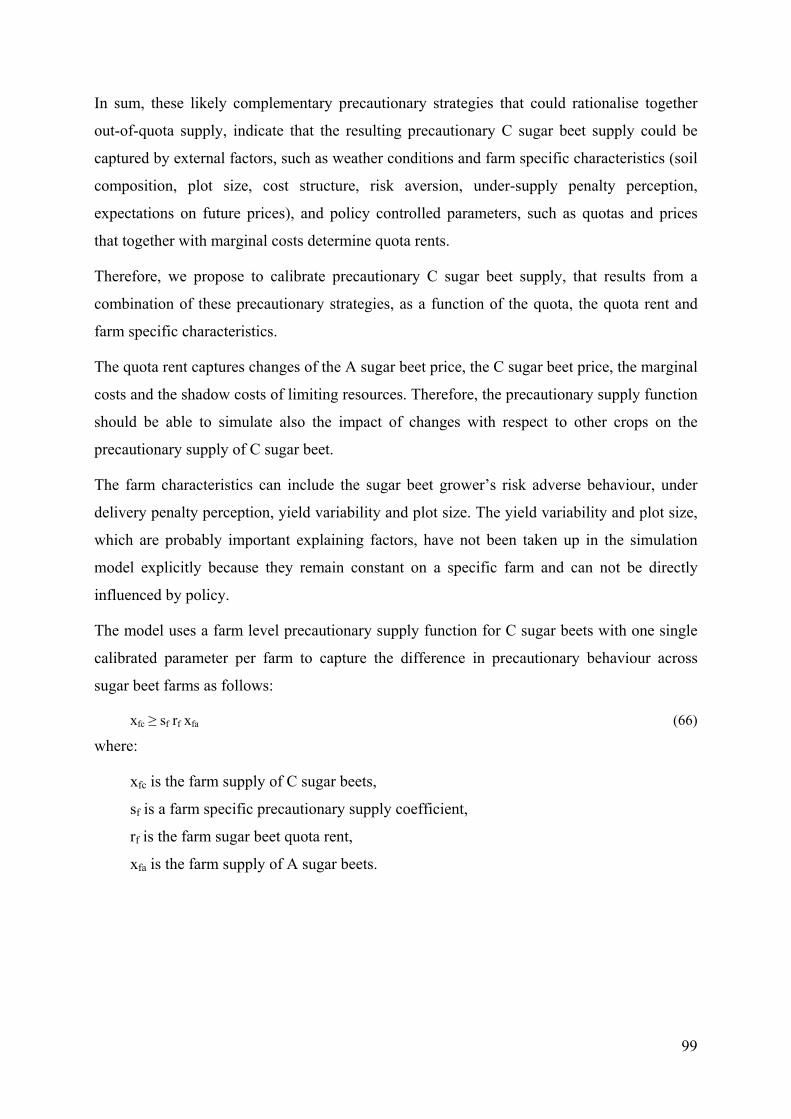
In sum, these likely complementary precautionary strategies that could rationalise together

out-of-quota supply, indicate that the resulting precautionary C sugar beet supply could be

captured by external factors, such as weather conditions and farm specific characteristics (soil

composition, plot size, cost structure, risk aversion, under-supply penalty perception,

expectations on future prices), and policy controlled parameters, such as quotas and prices

that together with marginal costs determine quota rents.

Therefore, we propose to calibrate precautionary C sugar beet supply, that results from a

combination of these precautionary strategies, as a function of the quota, the quota rent and

farm specific characteristics.

The quota rent captures changes of the A sugar beet price, the C sugar beet price, the marginal

costs and the shadow costs of limiting resources. Therefore, the precautionary supply function

should be able to simulate also the impact of changes with respect to other crops on the

precautionary supply of C sugar beet.

The farm characteristics can include the sugar beet grower’s risk adverse behaviour, under

delivery penalty perception, yield variability and plot size. The yield variability and plot size,

which are probably important explaining factors, have not been taken up in the simulation

model explicitly because they remain constant on a specific farm and can not be directly

influenced by policy.

The model uses a farm level precautionary supply function for C sugar beets with one single

calibrated parameter per farm to capture the difference in precautionary behaviour across

sugar beet farms as follows:

xfc ≥ sf rf xfa (66)

where:

xfc is the farm supply of C sugar beets,

sf is a farm specific precautionary supply coefficient,

rf is the farm sugar beet quota rent,

xfa is the farm supply of A sugar beets.

99

The farm level sugar beet profit function is then written in algebraic notation, extended with

the overall land constraint (70) in matrix notation, as follows:

П = pfa xfa + pfc xfc - qfs / 2 (xfa + xfc)² - dfs (xfa + xfc) (67)

subject to:

xfa ≤ mf [rf] (68)

xfc ≥ sf rf xfa [σf] (69)

f

F

f 1

a 'x=∑ f

f o

= [l] (70) f fo

F

f 1

a 'x=∑

where:

pfa is the farm A sugar beet price,

pfc is the farm C sugar beet price,

qfs is the farm quadratic cost function parameter of sugar beet,

dfs is the farm linear cost function parameter of sugar beet,

afs is the farm technical coefficient determining how much resource base (i.e., farmland)

is needed per production quantity of sugar beet,

mf is the farm sugar beet quota,

rf and σf are the dual variables from equations (68) and (69),

l is the dual variable from the overall land constraint (70) reflecting changes in land

price,

xfa ≥ 0; xfc ≥ 0; rf ≥ 0; σf ≥ 0.

To ensure the equality between the dual variable from the first constraint (68) and the rent

parameter in the second constraint (69), the programme is rewritten in terms of its

complementary slackness conditions as follows:

[pfa - qfs (xfa + xfc) - dfs - l afs - rf - σf ( sf rf ) ] xfa = 0 (71)

[pfc - qfs (xfa + xfc) - dfs - l afs + σf] xfc = 0 (72)

[mf - xfa] rf = 0 (73)

[xfc - sf rf xfa] σf = 0 (74)

f

F

f 1

a 'x=∑ - = 0 (75) f f

F

f 1

a 'x=∑

The price pfa and pfc are available from the baseline for calibration and exogenously

determined for simulation. The variables xfa and xfc, are the decision variables and the

variables r, σ and l are the duals of the sugar quota restriction, the precautionary supply

function and the overall land constraint respectively.

100

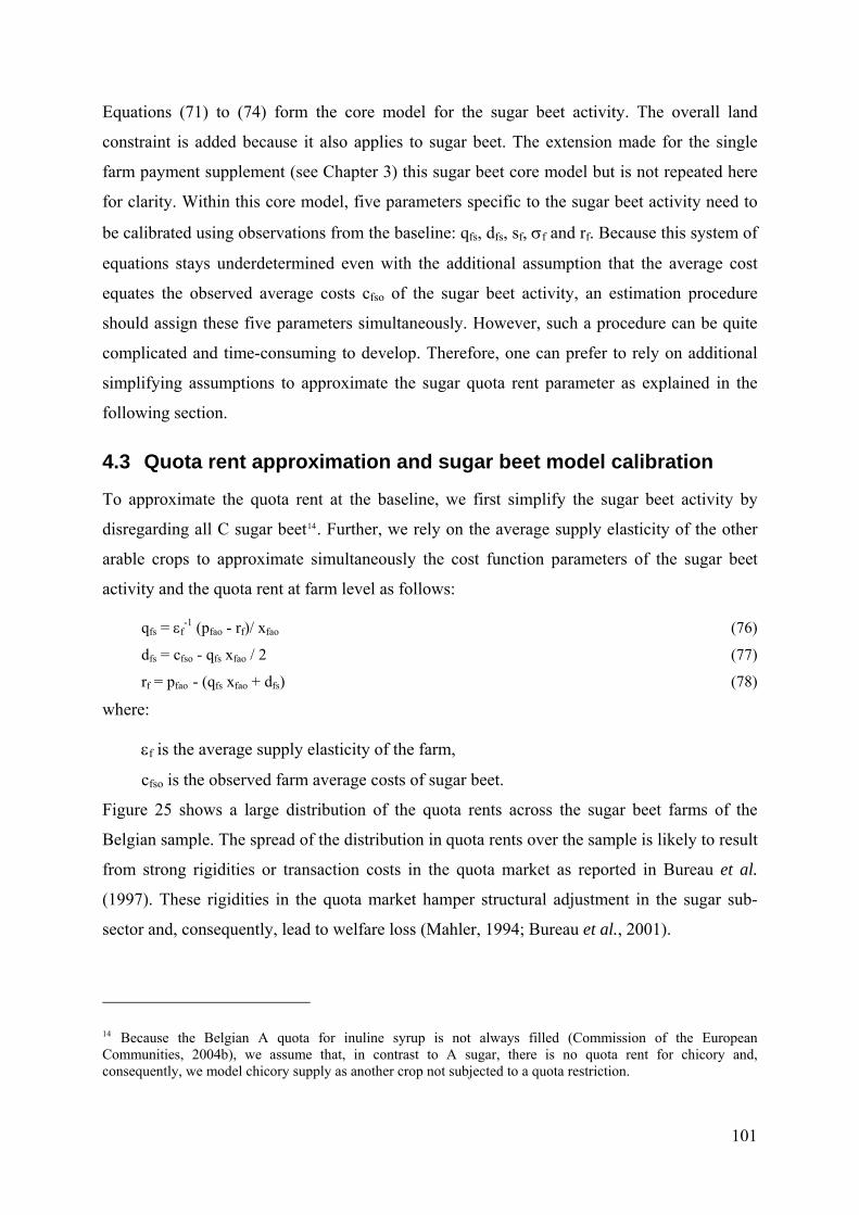
Equations (71) to (74) form the core model for the sugar beet activity. The overall land

constraint is added because it also applies to sugar beet. The extension made for the single

farm payment supplement (see Chapter 3) this sugar beet core model but is not repeated here

for clarity. Within this core model, five parameters specific to the sugar beet activity need to

be calibrated using observations from the baseline: qfs, dfs, sf, σf and rf. Because this system of

equations stays underdetermined even with the additional assumption that the average cost

equates the observed average costs cfso of the sugar beet activity, an estimation procedure

should assign these five parameters simultaneously. However, such a procedure can be quite

complicated and time-consuming to develop. Therefore, one can prefer to rely on additional

simplifying assumptions to approximate the sugar quota rent parameter as explained in the

following section.

4.3 Quota rent approximation and sugar beet model calibration

To approximate the quota rent at the baseline, we first simplify the sugar beet activity by

disregarding all C sugar beet14. Further, we rely on the average supply elasticity of the other

arable crops to approximate simultaneously the cost function parameters of the sugar beet

activity and the quota rent at farm level as follows:

qfs = εf-1 (pfao - rf)/ xfao (76)

dfs = cfso - qfs xfao / 2 (77)

rf = pfao - (qfs xfao + dfs) (78)

where:

εf is the average supply elasticity of the farm,

cfso is the observed farm average costs of sugar beet.

Figure 25 shows a large distribution of the quota rents across the sugar beet farms of the

Belgian sample. The spread of the distribution in quota rents over the sample is likely to result

from strong rigidities or transaction costs in the quota market as reported in Bureau et al.

(1997). These rigidities in the quota market hamper structural adjustment in the sugar sub-

sector and, consequently, lead to welfare loss (Mahler, 1994; Bureau et al., 2001).

14 Because the Belgian A quota for inuline syrup is not always filled (Commission of the European Communities, 2004b), we assume that, in contrast to A sugar, there is no quota rent for chicory and, consequently, we model chicory supply as another crop not subjected to a quota restriction.

101

0

1

2

3

4

5

6

7

8

9

10

1 6 11 16 21 26 31 quota rent (euro/tonne)

number of farms

0

50

100(%)

Number offarms/category

cumulativepercetage offarms

Figure 25. Distribution of the average quota rent estimates for sugar beets over the selected

sample of the Belgian FADN (1995-2002)

The median calculated quota rent of about 18 euro per tonne is 20% higher than the quota rent

of 15 euro that is implied in an opportunity cost for sugar beets of 30 euro per tonne derived

for Belgium in 1990 by Bureau et al. (1997) and an average price for quota sugar beets in

Belgium of about 45 euro per tonne.

The approximated quota rent is likely overestimated because the extra C sugar beet supply

results in higher marginal costs. In addition, the cost of the loss made on the C sugar beet

supply, σf, which reduces the quota rent is also not taken into account.

With the quota rent rf now externally calibrated thanks to the use of the average supply

elasticity of the farm, we can return to the core model (71) and (73) and calibrate the other

parameters qfs, dfs, sf and σf at the baseline. If, following expert opinions, we assume that C

sugar beets are only supplied for precautionary purposes as explained above, the dual σf is

strictly positive for every sugar beet farm of the sample at the baseline. Since, in addition, the

dual rf and the sugar beet supplies xfa and xfc are strictly positive for every sugar beet farm of

the sample at the baseline, we can solve the core model for the parameters qfs, dfs, sf and σf

adding up the average cost equation to the system.

Since the values of the calibrated parameters qfs, dfs, sf and σf largely depend on the externally

calibrated quota rent rf, a sensitivity analysis on the value of this calibrated quota rent is

performed at the end of the following section.

102

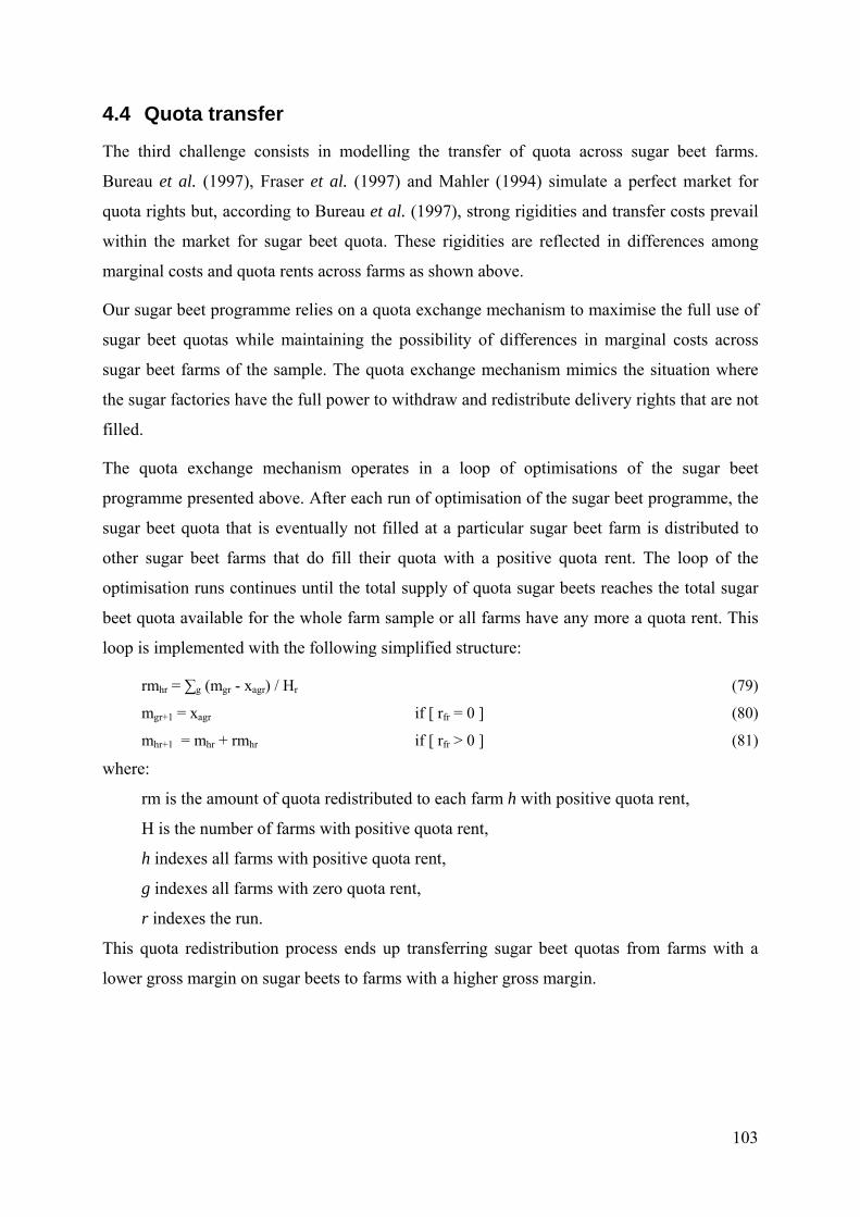
4.4 Quota transfer

The third challenge consists in modelling the transfer of quota across sugar beet farms.

Bureau et al. (1997), Fraser et al. (1997) and Mahler (1994) simulate a perfect market for

quota rights but, according to Bureau et al. (1997), strong rigidities and transfer costs prevail

within the market for sugar beet quota. These rigidities are reflected in differences among

marginal costs and quota rents across farms as shown above.

Our sugar beet programme relies on a quota exchange mechanism to maximise the full use of

sugar beet quotas while maintaining the possibility of differences in marginal costs across

sugar beet farms of the sample. The quota exchange mechanism mimics the situation where

the sugar factories have the full power to withdraw and redistribute delivery rights that are not

filled.

The quota exchange mechanism operates in a loop of optimisations of the sugar beet

programme presented above. After each run of optimisation of the sugar beet programme, the

sugar beet quota that is eventually not filled at a particular sugar beet farm is distributed to

other sugar beet farms that do fill their quota with a positive quota rent. The loop of the

optimisation runs continues until the total supply of quota sugar beets reaches the total sugar

beet quota available for the whole farm sample or all farms have any more a quota rent. This

loop is implemented with the following simplified structure:

rmhr = ∑g (mgr - xagr) / Hr (79)

mgr+1 = xagr if [ rfr = 0 ] (80)

mhr+1 = mhr + rmhr if [ rfr > 0 ] (81)

where:

rm is the amount of quota redistributed to each farm h with positive quota rent,

H is the number of farms with positive quota rent,

h indexes all farms with positive quota rent,

g indexes all farms with zero quota rent,

r indexes the run.

This quota redistribution process ends up transferring sugar beet quotas from farms with a

lower gross margin on sugar beets to farms with a higher gross margin.

103

4.5 Calibration and simulation results

Simulations are performed on an FADN subsample of 117 Belgian sugar beet farms

specialised in arable crops, each producing more than 2 ha of sugar beet. Only farm activities

that account for more than 0,5% of the farm gross margin are included in the model and the

simulation runs.

Table 6 illustrates the representativeness of the sugar beet farm sample with respect to its

population of origin. As a result of the sample selection, the average crop and sugar beet area

and the average share of sugar beet area in crop area are higher for the sample than for the

population. That the average share of C sugar beet supply for the population is higher than for

the sample implies that sugar beet farms growing less than 2 ha of sugar beets generally

supply a higher proportion of C sugar beets that the others, strengthening our assumption

about the existence of a farm specific precaution parameter.

Table 6. Comparison of sample and population for the 2002 calibration year

Farm characteristics Sample PopulationNumber of sugar beet farms 117 14 065 Average crop area per farm (ha) 52,8 40,06 Average sugar beet area per farm (ha) 10,5 6,8 Average share of sugar beet area in crop area (%) 21,7 17,0 Average sugar beet yield (T/ha) 65,7 67,7 Average share of C sugar beet supply in total sugar beet supply (%)

12,7 18,4

Sources: FADN and Belgian National Institute for Statistics

Table 7 shows the characteristics of the sample in terms of crop area share, yield and price

reported by crops. Besides sugar beets, most sugar beet farms from the sample supply winter

cereals, followed by fallow, potatoes, chicory and then summer cereals. The average share of

area is the highest for winter cereals (27,4%), followed by potatoes (13,8%) wet pulses

(10,9%) and then sugar beets (10,5%). The variability around these averages is high across the

sample, in particular for potatoes. The variability around the average yields and prices is

particular high for industrial and the other arable crops because these categories include

diverse crops.

104

Table 7. Farm characteristics of the sample for the 2002 calibration year

Area ( % ) Yield (tonne/ha) Price (€/tonne)

Crop # farms average st. deviation across farms average

st. deviation across farms average

st. deviation across farms

Total sugar beet 117 9,4 7,9 65,8 6,7 50,5 2,9C sugar beet 117 1,1 0,7 65,8 6,7 11,0 1,9Winter cerealsa 115 27,4 19,6 8,3 0,9 105,6 15,3Summer cerealsb 24 5,6 4,7 6,4 1,5 108,9 31,5Maize 11 4,1 3,1 10,7 1,6 102,6 39,1Wet pulses 17 10,9 7,2 9,8 3,1 208,5 41,0Potatoes 42 13,8 20,7 42,4 9,5 78,0 46,1Chicory 40 8,1 5,1 43,2 6,1 50,2 6,8Industrial cropsc 4 7,3 4,9 3,9 2,9 1141,7 899,6Other arable cropsd 17 8,4 6,7 29,7 29,5 252,3 430,2Fallowe 71 5,1 2,9 0,7 1,1 249,6 83,9

(a): includes winter wheat and winter barley, (b): includes all other cereals e.g. summer wheat, (c): includes flax and hop, (d): includes grass seeds, Belgian endive, vegetables in open air, (e): includes rapeseed, other non-food crops on fallow and set-aside. Source: FADN

The year 2002 is chosen as the calibration year. To take the yield variations for sugar beet into

account the calibration data for sugar beet are based on averages of 1995 to 2002. Table 8

reports the resulting values of the calibrated parameters of the quadratic cost function and

their respective supply elasticities implied by the cost function15.

Table 8. Calibrated cost function parameters and supply elasticities from the FADN crop farm sample

Crop Linear cost parameter

Quadratic cost parameter

Supply elasticity

Average Average Average St. deviationWinter cereals 33,6 0,5 1,1 0,9Summer cereals 34,8 3,4 1,0 0,9Maize 16,6 2,7 1,0 0,4Wet pulses 34,3 1,8 1,4 1,0Potatoes -7,2 0,1 1,3 1,1Chicory 3,7 0,1 1,2 0,6Industrial crops 44,4 28,9 1,1 0,2Other arable crops -15,8 31,3 1,1 1,5Fallow 177,9 206,5 1,1 1,2

15 The simulated supply elasticities can be different due to the competition for the limited resource land.

Generally, the simulated supply elasticities are lower. That difference increases for crops with a larger share in

the total acreage.

105

Simulations are based on the calibrated profit function, but with two additional decision

variables for the supply of A and C sugar beets as in the profit function (67) and the sugar

beet constraints (68) and (69), extended with the sample land constraint, the quota and the

precautionary supply constraints, the single farm payment and the fallow constraints. This

farm model is completely re-written in complementary slackness conditions in which the

equality between the dual 'rf' of the quota constraint (68) and the quota rent in equation (69) is

imposed. This farm model in Mixed Complementary Problem (MCP) form is optimised with

the Path solver from GAMS. After each optimisation run of the 117 farm models the equation

system (79) to (81) is executed consecutively. This process is repeated until the aggregate

supply of A sugar beets equal the quota available to the farm sample.

The reference scenario corresponds to the full implementation of the June 2003 CAP reform

with full decoupling of direct payments for cereal, oilseed and protein (COP) crops as agreed

upon in Belgium. Table 9 summarises the observed supply levels in 2002 and the simulated

supply levels from the implementation of the June 2003 CAP reform. Simulation results from

the reference scenario show that the implementation of the single payment with complete

decoupling of COP direct subsidies leads to a decline in the supply of the previously

subsidised crops such as cereals and maize, and to a supply increase of most other crops.

Supply of C sugar beets increases by 18%, due to the increase in precautionary supply as a

result of increased quota rents. Supply of A sugar beets is constrained by quota and, therefore,

remains constant with respect to the calibration year.

Table 9. Changes in the aggregate crop supply as a result of the June 2003 CAP reform

Crop 2002 supply (tonne)June 2003 CAP reform scenario supply (tonne) Variation (%)

Total sugar beet 79579,4 81640,1 2,6A sugar beet 71294,0 71294,0 0,0C sugar beet 8285,4 10346,2 24,9Winter cereals 25549,2 23801,2 -6,8Summer cereals 818,8 738,2 -9,8Maize 528,5 485,8 -8,1Wet pulses 1772,8 2196,8 23,9Potatoes 24506,1 27978,6 14,2Chicory 14014,5 14014,5 0,0Industrial crops 148,3 164,8 11,1Other arable crops 3935,6 4325,8 9,9Fallow 251,8 259,3 3,0

106

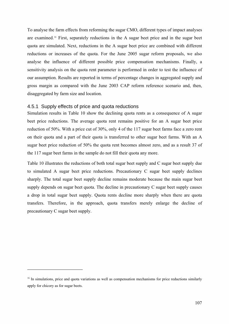
To analyse the farm effects from reforming the sugar CMO, different types of impact analyses

are examined.16 First, separately reductions in the A sugar beet price and in the sugar beet

quota are simulated. Next, reductions in the A sugar beet price are combined with different

reductions or increases of the quota. For the June 2005 sugar reform proposals, we also

analyse the influence of different possible price compensation mechanisms. Finally, a

sensitivity analysis on the quota rent parameter is performed in order to test the influence of

our assumption. Results are reported in terms of percentage changes in aggregated supply and

gross margin as compared with the June 2003 CAP reform reference scenario and, then,

disaggregated by farm size and location.

4.5.1 Supply effects of price and quota reductions Simulation results in Table 10 show the declining quota rents as a consequence of A sugar

beet price reductions. The average quota rent remains positive for an A sugar beet price

reduction of 50%. With a price cut of 30%, only 4 of the 117 sugar beet farms face a zero rent

on their quota and a part of their quota is transferred to other sugar beet farms. With an A

sugar beet price reduction of 50% the quota rent becomes almost zero, and as a result 37 of

the 117 sugar beet farms in the sample do not fill their quota any more.

Table 10 illustrates the reductions of both total sugar beet supply and C sugar beet supply due

to simulated A sugar beet price reductions. Precautionary C sugar beet supply declines

sharply. The total sugar beet supply decline remains moderate because the main sugar beet

supply depends on sugar beet quota. The decline in precautionary C sugar beet supply causes

a drop in total sugar beet supply. Quota rents decline more sharply when there are quota

transfers. Therefore, in the approach, quota transfers merely enlarge the decline of

precautionary C sugar beet supply.

16 In simulations, price and quota variations as well as compensation mechanisms for price reductions similarly

apply for chicory as for sugar beets.

107

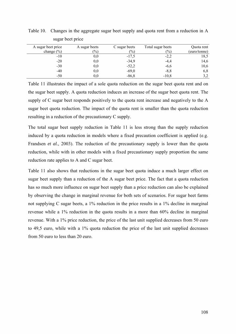
Table 10. Changes in the aggregate sugar beet supply and quota rent from a reduction in A

sugar beet price A sugar beet price

change (%) A sugar beets

(%)C sugar beets

(%)Total sugar beets

(%) Quota rent

(euro/tonne)-10 0,0 -17,5 -2,2 18,5-20 0,0 -34,9 -4,4 14,6-30 0,0 -52,2 -6,6 10,6-40 0,0 -69,0 -8,8 6,8-50 0,0 -86,8 -10,8 3,2

Table 11 illustrates the impact of a sole quota reduction on the sugar beet quota rent and on

the sugar beet supply. A quota reduction induces an increase of the sugar beet quota rent. The

supply of C sugar beet responds positively to the quota rent increase and negatively to the A

sugar beet quota reduction. The impact of the quota rent is smaller than the quota reduction

resulting in a reduction of the precautionary C supply.

The total sugar beet supply reduction in Table 11 is less strong than the supply reduction

induced by a quota reduction in models where a fixed precaution coefficient is applied (e.g.

Frandsen et al., 2003). The reduction of the precautionary supply is lower than the quota

reduction, while with in other models with a fixed precautionary supply proportion the same

reduction rate applies to A and C sugar beet.

Table 11 also shows that reductions in the sugar beet quota induce a much larger effect on

sugar beet supply than a reduction of the A sugar beet price. The fact that a quota reduction

has so much more influence on sugar beet supply than a price reduction can also be explained

by observing the change in marginal revenue for both sets of scenarios. For sugar beet farms

not supplying C sugar beets, a 1% reduction in the price results in a 1% decline in marginal

revenue while a 1% reduction in the quota results in a more than 60% decline in marginal

revenue. With a 1% price reduction, the price of the last unit supplied decreases from 50 euro

to 49,5 euro, while with a 1% quota reduction the price of the last unit supplied decreases

from 50 euro to less than 20 euro.

108

Table 11. Changes in the aggregate sugar beet supply and quota rent from a reduction in sugar

beet quota Quota change

(%) A sugar beets

(%)C sugar beets


(%) Quota rent

(euro/tonne)-10 -10 -0,4 -8,8 24,9-20 -20 -2,2 -17,8 27,5-30 -30 -5,8 -26,9 30,2-40 -40 -11,3 -36,4 33,0-50 -50 -19,0 -46,0 36,0

4.5.2 Supply effects of a combined price reduction and quota reduction or increase

Figure 26 shows that the effects of a combined reduction in price and quota on sugar beet

supply are much weaker than the sum of the separated effects of the reductions in price and

quota. As observed in Table 10, the impact of a price reduction is larger when the quota rent

decreases and reaches zero. Because the quota rent increases when quota decreases, adding a

combined price reduction to a quota reduction only slightly aggravates the impact on sugar

beet supply.

-55

-50

-45

-40

-35

-30

-25

-20

-15

-10

-5

0

0 10 20 30 40 50price and/or quota

reduction (%)

Change in Supply (%)

pricereduction

quotareduction

price andquotareduction


aggregate supply of sugar beet

109

Table 7 shows the effects of an increase in sugar beet quota combined with a reduction in the

A sugar beet price. This is what would happen if the Belgian sugar factories decide to buy

additional quota. Such increase in quota combined with a reduction in the price induces an

increase in total supply of sugar beets. As a result of the increase in available quota, sugar

beet suppliers, however, shift their sugar beet production towards A sugar beets and the

supply of precautionary C sugar beets declines as a result of the quota rent reduction. For a

quota increase of more than 40% combined with a price reduction of more than 40%, the

quota rent approaches zero. From that moment on, not the whole available quota is supplied

and total sugar beet supply starts to decline.

Table 12. Changes in aggregate sugar beet supply and quota rent from changes in sugar beet

quota and price A sugar beet

price change (%) Quota change

(%) A sugar beets

(%)C sugar beets


(%) Quota rent

(euro/tonne)-10 +10 10,0 -19,9 6,2 16,3-20 +20 20,0 -42,7 12,1 10,5-30 +30 30,0 -66,2 17,8 5,5-40 +40 40,0 -72,9 25,7 3,6

4.5.3 Supply effects of compensation mechanisms Figure 27 indicates the supply effects of compensating the A sugar beet price reduction with

coupled and, alternatively, decoupled direct acreage subsidies in case of a 39,5% reduction in

the A sugar beet price as has been agreed in November 2005 by the European Council. The

compensation is calculated as the A sugar beet price reduction multiplied by the quota

amount. 100% compensation can, therefore, in reality mean that farms are overcompensated

because they can adjust their farm plan. The compensation is, however, as all other subsidies

subject to modulation.

As expected, a coupled sugar beet subsidy mitigates the supply effect of the reduction in the

price. In contrast, a decoupled sugar beet subsidy comes as an addition to the total decoupled

subsidies that are granted to the farm according to its eligible area, i.e., all land not planted

with potatoes and vegetables. The decoupled direct payments have, in this sample of farms,

no supply inducing effect for sugar beet, because the eligible area is not the limiting factor for

activating decoupled payments.

110

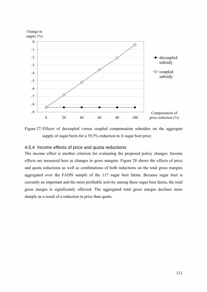
-9

-8

-7

-6

-5

-4

-3

-2

-1

0

0 20 40 60 80 100Compensation of

price reduction (%)

Change in supply (%)

decoupledsubsidy

coupledsubsidy

Figure 27. Effects of decoupled versus coupled compensation subsidies on the aggregate

supply of sugar beets for a 39,5% reduction in A sugar beet price

4.5.4 Income effects of price and quota reductions The income effect is another criterion for evaluating the proposed policy changes. Income

effects are measured here as changes in gross margins. Figure 28 shows the effects of price

and quota reductions as well as combinations of both reductions on the total gross margins

aggregated over the FADN sample of the 117 sugar beet farms. Because sugar beet is

currently an important and the most profitable activity among these sugar beet farms, the total

gross margin is significantly affected. The aggregated total gross margin declines more

sharply as a result of a reduction in price than quota.

111

-30

-25

-20

-15

-10

-5

0

0 10 20 30 40 50price and/or quota

reduction (%)

Change in gross margin (%)

pricereduction

quotareduction

price andquotareduction


aggregated total gross margin

Figure 29 shows the effects of compensating the A price reduction with coupled and,

alternatively, decoupled direct acreage subsidies on the aggregated gross margin of the

simulated FADN sample for a 39,5% reduction in the price. Decoupling the compensation

subsidies mitigates the decline in total gross margin because, for the same amount of

subsidies, sugar beet farms have more flexibility in allocating their activities to maximise

their total gross margins. The difference in gross margin between coupled and decoupled

subsidies is, however, very small. The simulation of the accepted EU sugar CMO reform

proposal in our model induces a decline of about 8% in aggregated total gross margin.

112

-20

-18

-16

-14

-12

-10

-8

-6

-4

-2

0

0 20 40 60 80 100Compensation of

price reduction (%)

Gro

ss m

argi

n (%

)

decoupledsubsidy

coupledsubsidy

Figure 29. Effects of decoupled versus coupled price reduction compensation subsidies on the

aggregated total sugar beet gross margin for a 39,5% reduction in price.

4.5.5 Supply effects on other crops Table 13 shows to what extent a price reduction compensation, whether coupled or not,

affects the supply of the other major crops of the sugar beet farms in case of a 39,5%

reduction in the price and a 64,2% compensation of the price reduction. This is what is

envisaged in the June 2005 proposal. As expected, a price reduction compensation coupled to

sugar beet acreage has not much additional influence on the supply of the other crops. In

contrast, a price reduction compensation decoupled of sugar beet acreage increases the supply

of the other crops, i.e., mainly cereals, maize and potatoes.

113


crops of sugar beet farms within the Belgian FADN for a 39,5% reduction in A sugar beet

price

Difference (%)

Crop Decoupled

CompensationCoupled

CompensationNo

compensation Total sugar beet -8,4 -3,3 -8,4 A sugar beet -23,2 -3,8 -23,2 C sugar beet 0,0 0,0 0,0 winter cereals 4,9 1,4 4,9 summer cereals 3,8 1,1 3,8 Maize 1,6 0,4 1,6 wet pulses 2,2 0,6 2,2 Potatoes 2,3 0,7 2,3 Chicory 4,6 1,4 4,6 industrial crops 0,1 0,0 0,1 other arable crops 5,0 1,5 5,0 Fallow -69,0 -27,1 -69,0

4.5.6 Supply and income effects according to farm size and region An advantage of our farm based modelling approach is that results can be disaggregated

according to certain farm characteristics such as location and farm size. Table 14 shows the

model results for different farm size classes and different regions. As can be derived from the

results, the supply mainly decreases on the smaller farms (L, M and S) which are mainly

located in Flanders. The Flemish farms have in general more opportunities for replacing the

sugar beet than the larger Walloon arable farms which have a smaller diversity of crops.

Table 14. Effects of the accepted sugar CMO reform according to size classes and regions Difference (%) supply gross margin

Size classes XXL -6,4 -2,5XL -7,4 -7,1L -9,3 -6,7M -11,8 -6,4S -10,9 -9,7

Regions Flanders -11,3 -4,8Wallonia -7,5 -7,2

4.5.7 Sensitivity analysis on the quota rent approximation Because we are aware that our approximation of the quota rent could be subject to discussion,

we show the impact on the final simulation results of different assumptions of the quota rent.

In the sensitivity analysis the quota rent varies from -20% to +20% of the initial value. The

results are compared for three scenarios: an A sugar beet price reduction of 40%, a quota

reduction of 20% and a combined price and quota reduction of 40% and 20%.

114

The results in Table 15 show that the impact of the varying initial quota rent on the total sugar

beet supply change is limited. A change in quota rent from -20% to +20% of the initial

approximation only changes the total supply reaction from -9,8% to -7,9% for the price

reduction, from -16,9% to -18,3% for the quota reduction and from -25,4% to -24,9% for the

combined price and quota reduction.

The most important explanation for this robustness is that the initial quota rent adjusts the

precaution behaviour reversely. A higher initial quota rent leads to a lower precaution

coefficient and therefore a smaller reaction of the C sugar supply to changes in quota and

quota rent.

Table 15. Changes in the aggregate sugar beet supply and quota rent from A sugar beet price

and quota reductions with different initial approximated quota rents Approximated

quota rent (%)

Quota change (%)

A sugar beet price change

(%)

A sugar beets (%)

C sugar beets (%)

Total sugar beets (%)

Quota rent (euro/tonne)

-20 0 -40 0 -75,1 -9,8 4,2-10 0 -40 0 -71,8 -9,3 5,5

0 0 -40 0 -69,1 -8,8 6,810 0 -40 0 -67,1 -8,3 7,820 0 -40 0 -65,9 -7,9 8,6

-20 -20 0 -20 4,0 -16,9 24,2-10 -20 0 -20 0,5 -17,3 25,9

0 -20 0 -20 -2,3 -17,8 27,510 -20 0 -20 -4,5 -18,1 28,720 -20 0 -20 -6,0 -18,3 30,3

-20 -20 -40 -20 -60,9 -25,4 9,0-10 -20 -40 -20 -61,0 -25,3 9,9

0 -20 -40 -20 -61,1 -25,2 10,910 -20 -40 -20 -61,3 -25,1 11,620 -20 -40 -20 -61,4 -24,9 12,4

115

4.6 Conclusions

4.6.1 Conclusions with respect to the application The economic behaviour of individual sugar beet farms in Belgium who are facing delivery

quota is represented in our model through an individual farm level profit function. The profit

functions of sugar beet farms consists of a decision variable for the supply of A sugar beets

within the delivery quota and a second decision variable for the supply of C sugar beets above

delivery quota. To represent the sugar beet farms' precautionary behaviour against

undersupply of their quota, a precautionary supply function is proposed. This precautionary

supply function simulates changes in C sugar beet supply as a result of changes in quota and

quota rent and takes the farm specific precautionary behaviour into account. From the first-

order profit maximising conditions, parameters of the individual quadratic cost function of the

profit function are calibrated to the base period. During simulations, individual quota rents are

calculated at farm level and drive exchanges of sugar quotas from sugar beet farms with lower

quota rents to sugar beet farms with higher quota rents.

Simulation results indicate that the aggregate sugar beet supply of the FADN sample is rather

inelastic to a reduction in A sugar beet price, but less so to a reduction in delivery quota.

These key results are in line with those obtained from the general equilibrium model of

Frandsen et al. (2003) that simplifies the economic behaviours of sugar beet farms into one

single representation per member state. However, the simulation results from the farm level

approach of our model show that a quota reduction is not completely transmitted into an

equivalent decline in aggregate sugar beet supply. Precautionary supply of C sugar decreases

less than the equivalent quota reduction.

Adding a price reduction to a quota reduction only slightly aggravates the decline in supply

from the quota reduction alone. Adding a price reduction to a quota increase generates an

increase in total sugar supply, but a reduction of precautionary supply out of quota.

Simulations of accepter sugar CMO reform of November 2005 that includes a 39,5%

reduction in the sugar beet price and a decoupled subsidy to compensate 64,2% of the

minimum sugar beet price cut reduces the aggregated sugar beet supply of the selected sample

by about 8,5% and total gross margin by about 6,6%.

116

These simulation results have important policy implications. If the aim of the policy reform

consists in reducing the Belgian sugar beet supply while preserving as much as possible sugar

beet farms' incomes, then a quota reduction should be preferred to a minimum sugar beet

price reduction. For example, a 10% decline in sugar beet supply requires either a quota

reduction of 13% or a minimum sugar beet price reduction of 46%. In the first case, the sugar

beet farms' gross margin declines by about 3% while in the second case by about 22%.

However, if the aim of the policy change consists in reducing significantly the sugar market

price while maintaining sugar beet supply, then a reduction in minimum sugar beet price

would reach that aim, but at the expense of a considerable farm income loss. For example, a

50% reduction in minimum sugar beet price incurs a decrease in farms’ gross margin of about

26%.

4.6.2 Modelling lessons Before reflecting on modelling lessons with respect to quota, a general observation must be

made to make a correct interpretation of the results possible. It should be noted that the

simulation results could be sensitive to the feed-back effects from the demand side as well as

the international trade effects from the expected increase in sugar imports from the least

developed countries as a result of the "Everything But Arms" concessions of the EU and other

challenges awaiting the EU at the current WTO round of negotiations. One avenue for further

development is therefore to link this farm model to an EU and world model. Currently, the

results should be interpreted rather as counterfactual for the antecedent assumptions regarding

the market price than as indicative for real future observations. This shortcoming is true for

most programming models in agricultural policy analysis and more specifically for all models

presented in this dissertation.

With respect to quota, a fist impression is that modelling quota in MP models is

straightforward, because the quota can be represented by a simple constraint. In farm-level

PMP models, three challenges should nevertheless be kept in mind: quota rent approximation,

the possibility for over- and undersupply and the quota transfers. With respect to these

challenges, the application gives following modelling lessons.

117

The basic approach of quantifying the quota rent is to use observed prices for quota

transactions. This approach is, of course, only useful and valid if there is a transparent market

for quota and if the transactions of quota are observed. If data on quota transactions and quota

prices are scarce, quota rent approximation can be complicated. The latter is true for the sugar

beet in Belgium. As a consequence, the quota rent in the model is obtained by using

additional assumptions, which may influence the final results. It would, therefore, be better to

simultaneously calibrate all sugar beet specific parameters to avoid the ad hoc assumptions

related to the quota rent. The sensitivity analysis has shown, however, that the results are

quite robust regarding different quota rent assumptions.

The possibility of oversupply is captured by a precautionary supply function. The application

has shown that the model simulates more flexible the impact of policy changes than models

with a fixed precaution behaviour (such as Frandsen et al., 2003). The precautionary supply

function and the cost function are, however, probably not yet flexible enough to capture all

elements of farm behaviour. The cost function has only two calibrated parameter per crop per

farm and the only interaction between crops is simulated through the common constraints

such as land and direct payments. The precautionary supply function has only one parameter

and the model, therefore, imposes a linear relationship between quota rent and C sugar beet

supply. The estimation of more complex flexible functions requires, however, more data and

more adequate estimation techniques.

Next chapter is devoted to an EMP approach to tackle the issues of quota rent approximation

and the calibration of a more flexible precautionary supply function.

The third challenge is the modelling of quota transfers. Quota transfers are driven by farm

heterogeneity and hampered by transaction costs. SEPALE incorporates the farm

heterogeneity through the farm-level optimisation, but little known on the transactions costs

of transfers of quota. Further research is needed to assess these transaction costs and

incorporate them in the model because they can be important for policy recommendation and

they can influence the results.

118

Chapter 5 EMP extension of SEPALE

Chapter 5 elaborates on EMP with an application of EMP to the sugar module developed in

previous chapter. EMP refers to a calibration process in which the first-order conditions have

non-zero degrees of freedom, in contrast to PMP where there are zero degrees of freedom.

The purpose of the application is to calibrate the parameters of the sugar module based on an

estimation procedure. The estimation procedure avoids that ad hoc assumptions have to be

made and makes it possible to use a more flexible functional form for the precautionary

supply function.

There are, however, different definitions and connotations for the terms calibration and

estimation. Therefore, before the presentation of application, the chapter first reflects on the

meaning of estimation and calibration and how they are used in the context of this

dissertation.

Chapter 5 also presents more detailed results on the sugar reform, based on different reactions

of 4 farm groups of the same sample used in Chapter 4. These farm groups are identified with

a cluster analysis established with quota rent and percentage C supply as base variables.

Parts of this chapter have been submitted as


Huylenbroeck, G. and Van Meensel, J. (2006). Farm based modelling of the EU sugar reform:

impact on Belgian sugar beet suppliers. Submitted.

119

5.1 Introduction

Instead of relying on an auxiliary LP program and on additional assumptions, apparent in

most PMP applications, Heckelei and Wolff (2003) suggest an alternative by the estimation of

a programming model based on its first-order optimality conditions. This approach, which is

called in this dissertation EMP (Buysse et al., 2006), is used to calibrate the sugar module of

our model. Before presenting the application, the introduction gives an overview of different

opinions on the meaning and the use of calibration and estimation in this case.

In the literature, there is no consensus on the definition and use of estimation and calibration.

Quah (1995) makes following caricature of the difference between calibrators and estimators.

Calibrators criticises standard econometric practices for being uninformative on important

questions and have chosen to use calibration as an alternative to standard statistical

estimation. They have chosen to apply not the standard diagnostic testing, but to use a

model’s operating characteristics to evaluate it. Estimators evaluate models using statistical or

aesthetic criteria unmotivated by economic reasoning.

Also Balistreri and Hillberry (2005), state that the distinction in connotation between

calibration and estimation originates from the different focus of the research. They delineate

the processes of model fitting to the data and the subsequent model analyses. The different

respective notions of calibration and estimation only become clear in the analysis of fitted

models as the degree of concentration on counterfactual simulation versus hypothesis testing.

Although there seems to be acrimony between calibrators and estimators (Quah, 1995), the

approaches are sometimes very alike, certainly in the stage of model fitting. E.g., Dawkins et

al. (2001) state with respect to model fitting: “Calibration is estimation, estimation is

calibration", a point which is widely recognized in the macroeconomic real-business-cycle

literature (Hoover, 1995). Both calibration as estimation fit model to data (Balistreri and

Hillberry, 2005). The terms calibration and estimation have, furthermore, technical meanings

that are sufficiently general that each could contain the other (Quah, 1995).

According to these different views on calibration and estimation, which mainly come from the

literature of real business cycle economics, the approach introduced by Heckelei and Wolff

(2003), ‘estimation of constrained optimisation models’ also belongs to the branch of

calibrated models because of the focus on model fitting instead of hypothesis testing. The

same holds for all MP approaches presented in this dissertation.

120

The difference that we make between PMP and EMP could, therefore, be subject to

discussion. We define PMP and EMP models as follows.

The parameters of both PMP and EMP models are chosen to guarantee that the model

precisely mimics some particular feature of the historical data and, as a consequence, both

PMP and EMP models are calibrated.

According to our definition, a model belongs to the class of PMP models when its parameters

are assigned from the optimality conditions with zero degrees of freedom. In case of non-zero

degrees of freedom additional parameters are quantified from casual empiricism or unrelated

econometric studies or simplifying assumptions.

Conversely, the optimality conditions of an EMP model do not have zero degrees of freedom

and, therefore, a minimisation algorithm is used to adjust the simulation model’s parameters

such that the simulated output deviates minimally from the real output.

The definitions used in this dissertation and in Buysse et al. (2006) do also not completely

correspond to other definitions. E.g., Heckelei and Britz (2005) define the use of phase 1 of a

defining character of PMP and call the newly developed approaches ‘alternative approaches

to calibration and estimation or programming models’. According to that definition, Judez et

al. (2001) and SEPALE are no PMP methods, while they have been published as PMP

variants. For that reason, and to make the difference with EMP a bit clearer, we have chosen

to use a broader definition for PMP than Howitt (1995a) and Heckelei and Britz (2005).

More important than the definition, the differences and similarities between different

modelling approaches PMP and EMP should become clear. To illustrate the differences

between PMP and EMP, the remainder of the chapter presents an EMP version of the sugar

module of SEPALE.

5.2 Application: estimation of the C sugar beet precaution supply function

Previous chapter has concluded with the need for a simultaneous estimation of the optimality

conditions of the sugar module. This estimation has two advantages. First, the simplifying

assumptions for calibration are not needed anymore and the estimation allows for a more

flexible functional form of the precautionary supply function.

121

In the EMP version of the sugar module, we propose therefore a quadratic functional form of

the farm level precautionary supply function for C sugar beets as a function of the quota rent

with calibrated parameters s0 and s1 per farm to capture the difference in the precautionary

behaviours across sugar beet farms as follows:

xfc/xfa ≥ s0f rf + s1f r²f (82)

where:

s0f is a farm specific precautionary supply coefficient,

s1f is a farm specific precautionary supply coefficient,

The programme in terms of its complementary slackness conditions is as follows:

[pfa - qfs (xfa + xfc) - dfs - l afs - rf - σf (s0f rf + s1f r²f )] xfa = 0 (83)

[pfc - qfs (xfa + xfc) - dfs - l afs + σf] xfc = 0 (84)

[mf - xfa] rf = 0 (85)

[xfc/xfa - s0f rf - s1f r²f] σf = 0 (86)

f

F

f 1

a 'x=∑ f o - = 0 (87) f f

F

f 1

a 'x=∑

Within this core model, six parameters specific to the sugar beet activity need to be calibrated

using observations from the baseline: qfs, dfs, s0f, s1f, σf and rf. The procedure to estimate

these unknown parameters is based on the approach proposed by Heckelei and Wolff (2003)

and is presented in next subsection.

Heckelei and Wolff (2003) have used Generalized Maximum Entropy (GME) (Golan et al.,

1996), but they acknowledge that for their application, Ordinary Least Squares (OLS) could

have been applied as well. We have also chosen to apply GME, because Golan et al. (1996; p.

192 - 200) show, with preliminary sampling experiments, that the GME-data formulation has

lower MSE than other estimators for a simultaneous equations estimation as in this case. In

addition, GME allows for nonlinear relationships in parameters in the model. GME has,

however, three disadvantages for this application.

122

The first disadvantage is that GME offers fewer possibilities for performing statistical tests

than traditional econometric techniques such as OLS. While test statistics could add to the

utility of the entropy approach, it should be noted that the philosophy of the entropy

estimation approach within such a framework does not heavily emphasises hypothesis testing.

The focus is on using all available information to estimate and calibrate the unknown

parameters of the programming model. Once these parameters are obtained, based on all

available information from theory, data, and prior experience in the estimation procedure,

information theory dictates to use all, significant or not, the parameter estimates in the

simulation model. Doing anything else would imply the existence of additional information -

a possibility that has already been ruled out (Arndt et al., 2002).

The second disadvantage is that there is no closed form solution for the estimation. Heckelei

and Britz (2005) describe computational problems that can be expected from a GME

estimation of equations (83) to (87). A first possible solution is to use the Mathematical

Programming with Equilibrium Constraints (MPEC) solver in GAMS, which is still in

development. For the estimation of the sugar beet module in Belgium, it is easier to make in

advance the assumptions that the quota constraint (68) and the precautionary supply constraint

(82) are binding, which are important computational simplifications (for more details on the

computational problems see Heckelei and Britz, 2005).

The third disadvantage of GME is the need of support point intervals for the estimated

parameters and errors that can introduce a possible bias in the estimation results. The

following three courses of action can minimize the impact of the support points on the results.

First, a number of parameters and equations are eliminated by substitution. Second, we

impose a common parameter d across the sample. Third, very wide support ranges for the

estimated parameters reduce the influence of the centre of the support interval on the obtained

result.

123

The estimation is performed on unbalanced panel data of the same sample of 117 farms that

have been used in Chapter 4, with observations from 1995 to 2003. We assume that the farm

technology is captured by its cost function (parameters d and q) and that technology remains

constant for each individual farm. Therefore, q and d are time independent. q is farm

dependent to capture differences in technology between farms and d is common across the

sample to capture the common part of the technology17. The farms have the possibility to

supply a different quantity of sugar beet in the different years (changes on the marginal cost

function). This variation of quantities results in changes of marginal costs and quota rents,

which are, therefore, farm and time dependent. Finally, the precaution function parameters s0,

s1 are chosen to be farm dependent but invariant in time.

The choice of support points and the complexity of the estimation are simplified by the

elimination of the parameter q and σ in the system of equations as follows:

paf,t - 2 cof,t + d - rf,t + (pcf,t - 2 cof,t + d) (s0f rf,t + s1f rf,t² ) = 0 (88)

xcf,t - s0f rf,t mf,t - s1f rf,t² mf,t = 0 (89)

In order to capture the weather effects on the supply of C sugar beet, the parameter wt and

year dummies Tt are added to the precautionary supply function. Together with two error

terms, following estimation equations are proposed:

paf,t - 2 cof,t + d - rf,t + (pcf,t - 2 cof,t + d) (s0 rf,t + s1f r²f,t) + e1f,t = 0 (90)

xcf,t / mf,t - s0f rf,t - s1f r²f,t + wt Tt + e2f,t = 0 (91)

17 It is more common in panel estimation to assume a common slope 'q' instead of a common intercept 'd'.

However, with a farm independent parameter 'q' across the sample, we impose that supply elasticities 'ε' vary

extensively among farms as a consequence of large differences in supplied quantities among farms in the sample

(elasticity = 1/q * price/quantity). An additional motivation to choose a common parameter 'd' instead of a

common parameter 'q', is that a common parameter 'q' mathematically leads to lower rents and a lower elasticity

on larger farms than smaller farms. A common parameter 'd' does not impose any differences on rents or

elasticities that depend on structural differences among farms.

124

To obtain a calibrated model, additional restrictions prevent negative quota rents, a decreasing

marginal cost function and a decreasing precautionary supply as a function of the quota rent.

The GME estimation is performed as proposed by Golan et al. (1996). We estimate

unobserved frequencies pdk, prk,f,t, ps0k,f, ps1k,f, pe1k,f,t, pe2k,f,t, pwk,t that represent the data

generating process of respectively d, rf,t, s0f, s1f, e1f,t, e2f,t, wt. Therefore, we have to define

the support points zdk, zrk,f,t, zs0k,f, zs1k,f, ze1k,f,t, ze2k,f,t and zwk,t of the parameters rf,t, s0f, s1f,

e1f,t, e2f,t and wt respectively. The number of support point, k, for each parameter and error

term is 2. The support intervals for the parameters are [-1000;1000] for d and r and [-100;100]

for s0, s1, and w, and [-40;40] for e1 and [-0,5;0,5] for e2.

The estimation is executed with GAMS software and the CONOPT solver as follows:

Max H = - ∑k pdk ln(pdk) - ∑k,f,t prk,f,t ln(prk,f,t) - ∑k,f ps0k,f ln(ps0k,f) - ∑k,f ps1k,f ln(ps1k,f)

- ∑k,f,t pe1k,f,t ln(pe1k,f,t) - ∑k,f,t pe2k,f,t ln(pe2k,f,t) - ∑k,f pwk,t ln(pwk,t) (92)

subject to :

paf,t - 2 cof,t + d - rf,t + (pcf,t - 2 cof,t + d) (s0f rf,t + s1f r²f,t) + e1f,t = 0

xcf,t / mf,t - s0f rf,t - s1f r²f,t + wt Tt + e2f,t = 0

s0f mf,t + 2 s1f rf,t mf,t > 0

d < cof,t

d = ∑k zdk pdk

rf,t = ∑k zrk,f,t prk,f,t

s0f = ∑k zs0k,f ps0k,f

s1f = ∑k zs1k,f ps1k,f

e1f,t = ∑k ze1k,f,t pe1k,f,t

e2f,t = ∑k ze2k,f,t pe2k,f,t

wt = ∑k zwk,t pwk,t

1 = ∑k pdk

1 = ∑k prk,f,t

1 = ∑k ps0k,f

1 = ∑k ps1k,f

1 = ∑k pe1k,f,t

1 = ∑k pe2k,f,t

1 = ∑k pwk,t

Table 16 presents some average values and standard deviation of the resulting estimated

parameters. The average value of the quota rent en the cost function imply that the cost

function for sugar beet is flatter than for other crops.

125

The average value of the precaution parameters s0 and s1 are both negative. The average

percentage of C sugar beet is, however, positive on every farm. This implies that s1 is more

negative on farms with a low quota rent and s0 is more negative on farms with a higher quota

rent. The standard deviation of s0 and s1 show that there is much variation in the

precautionary behaviour among farms.

Table 16. Key results of the estimation of the sugar module Parameter average st. deviation r 20,4 7,8 d 8,58 0 s0 -0,059 0,33 s1 -0,0022 0,075

Figure 30 shows the distribution of the resulting estimated average quota rents across the

sugar beet farms of the Belgian sample.

0

2

4

6

8

10

12

1 6 11 16 21 26 31 quota rent (euro/tonne)

number of farms

0

50

100

(%)

Number offarms/category

cumulativepercetage offarms

Figure 30. Distribution of the approximated average quota rents for sugar beets over the

selected sample of the Belgian FADN (1995-2002)

The median calculated quota rent of about 20 euro per tonne is higher than the approximated

quota rent of 18 euro of the PMP application. The main reason is that the estimated cost

function is flatter than the PMP approximation.

A sensitivity analysis reported in Table 17 of the support intervals shows that the parameter

estimates 'ds', 'qsf' and 'rf' are robust with respect to the choice of the support intervals.

Conversely, the average values of the parameter estimates 's0f' and 's1f' are quite sensitive to

different support intervals due mainly to multicollinearity between ρft and ρ²ft.

126

Table 17. GME parameter estimates of the sugar

beet programme from a sensitivity analysis on the support intervals Intervals rf d qf s0f s1f

Average 16,0 8,00 0,027 -0,016 -0,002Narrower support intervals for the parameters: [-100;100] for d and rf,t, and [-10;10] for s0f, s1f and wt

St. deviation 6,8 0,00 0,091 0,140 0,046

Average 20,6 8,58 0,025 -0,028 0,002Wider support intervals for e2f,t: [-1;1]

St. deviation 7,6 0,00 0,085 0,150 0,007

Average 19,9 8,58 0,025 -0,052 0,009Wider support intervals for e1f,t: [-80;80]

St. deviation 7,9 0,00 0,085 0,530 0,031

5.3 Calibration and simulation results

The same reference scenario of the PMP application in Chapter 4 is used. Table 9 summarises

the observed supply levels in 2002 and the simulated supply levels from the implementation

of the June 2003 CAP reform. Supply of C sugar beets increases here by 54%, which is higher

than the 18% of the PMP application. On most farms this is due to the increase in

precautionary supply as a result of increased quota rents. On three farms, however, the

decrease of the land rent makes C sugar beet supply profitable. Due to the flat cost function

for sugar beet and the A sugar beets quota, the C sugar beet supply increases very much. The

increase of total sugar beet supply is, nevertheless, lower than the increase of supply of wet

pulses, potatoes and industrial crops.

Table 18. Changes in the aggregate crop supply as a result of the June 2003 CAP reform

Crop 2002 supply (tonne)June 2003 CAP reform scenario supply (tonne) Variation (%)

Total sugar beet 89168,0 97649,8 9,5A sugar beet 78895,2 78895,2 0,0C sugar beet 10272,8 18754,6 82,6Winter cereals 25549,2 23134,2 -9,5Summer cereals 818,8 717,5 -12,4Maize 528,5 476,2 -9,9Wet pulses 1772,8 2173,8 22,6Potatoes 24506,1 27784,1 13,4Chicory 14014,5 14014,5 0,0Industrial crops 148,3 163,9 10,5Other arable crops 3935,6 4303,9 9,4Fallow 251,8 255,6 1,5

127

5.3.1 Identification of farm groups One of the advantages of farm-level modelling is that results can be differentiated according

to farm type. To show the impact on different types of farms and to illustrate the underlying

economic mechanisms driving the aggregated outcome, four farm groups are identified with a

k-means cluster analysis18. The cluster analysis is based on two variables of importance for

the changes in sugar beet supply, the quota rent and percentage of C sugar beet supply. The

farm segregation is reported in Figure 31.

0

0,05

0,1

0,15

0,2

0,25

0,3

0,35

0,4

0,45

0,5

0 5 10 15 20 25 30 35 40 quota rent

Xc/Xa

Group 1

Group 2

Group 3

Group 4

Figure 31. Farm segregation from a k-means cluster analysis based on the quota rent and the percentage C sugar supply

Group 1 represents 6 farms with a low quota rent and a high percentage of C sugar beet

supply in the total sugar beet supply. Table 19 indicates that the farms of group 1 are equally

divided over the Walloon region and the Flemish region. Table 20 shows that the farms in

group 1 have on average 29,2 ha, which is the smallest of the 4 farm groups.

18 To perform a k-means cluster analysis, one has to specify the number of clusters and optionally the centres of

the clusters (otherwise they are randomly initialised). Each observation in the data set is then assigned to a

cluster based on its smallest Euclidian distance to the cluster centre. After the complete data set is assigned, new

cluster centres are calculated as the average positions of the data points within each cluster. This process of

assigning and averaging is repeated until the cluster centres converge. The cluster analysis is executed on

standardised variables.

128

Group 2 represents 27 farms with a higher quota rent than group 1 and a high percentage of C

sugar beet. The farms of group 2 are mainly located in the Walloon region. The farms of

group 2 are, with 39,9 ha, larger than the farms of group 1.

The high percentage of C sugar beet indicate that groups 1 and 2 are more risk averse with

respect to quota under filling than the farms in group 3 and 4. This risk averse behaviour is

also reflected in the lower acreage of potatoes, a crop with a high gross margin but with

volatile yields and prices.

Group 3 consists of primarily Flemish farms with the lowest quota rent and percentage C

sugar beet supply. The 38 farms of group 1 cultivate on average 52,6 ha, of which 9 ha is

allocated to potatoes.

The largest group 4, with 46 farms, contains mainly Walloon farms with a high quota rent and

a low percentage C sugar beet supply. The farms of group 4 are the largest, with 66.7 ha, and

are, more than the farms of the other groups, also involved with chicory production.

The Flemish farms can for the most part be found in the farm groups with a lower quota rent,

1 and 3. The lower rent at these farms can be explained by the larger acreage of crops with a

high gross margin and the higher land price than at the farms in group 2 and 4.

Table 19. Distribution of the farms over the different regions

Region Group 1 Group 2 Group 3 Group 4FLPO 1 1 6 2FLCA 0 0 1 0FLSL 1 1 8 2FLLO 1 1 6 1Flemish region 3 3 21 5WASL 0 3 1 6WALO 2 16 11 28WACO 1 5 3 5WAHL 0 0 0 1WAFF 0 0 2 1Walloon region 3 24 17 41Total 6 27 38 46

129

Table 20. Average acreage of different crops for the 4 farm groups (in ha)

Crop Group 1 Group 2 Group 3 Group 4Total sugar beet 6,7 9,0 11,1 14,3A sugar beet 4,7 7,2 10,2 12,8C sugar beet 2,0 1,8 0,8 1,4Winter cereals 17,4 23,1 23,3 33,4Summer cereals 0,0 1,4 0,8 1,4Maize 0,0 0,0 0,6 0,5Wet pulses 0,0 0,0 1,1 3,1Potatoes 1,5 1,1 9,0 4,3Chicory 0,7 1,6 1,2 5,1Industrial crops 0,7 0,0 0,7 0,0Other arable crops 0,6 0,9 1,8 1,1Fallow 1,6 2,7 3,0 3,6Total 29,2 39,7 52,6 66,7

Table 21 gives an overview of the differences precautionary behaviour between the four farm

groups. The farms of group 1 and 2 have a steep precautionary supply as function of the quota

rent. That function is concave for group 1 and convex for group 2. The precautionary supply

function of group 3 and 4 is also convex but flatter that the functions of group 1 and 2.

Table 21. Average precaution parameters for the 4 farm groups

Group 1 Group 2 Group 3 Group 4

average st.

deviation average st.



deviation s0 0,30 0,57 -0,24 0,54 -0,0039 0,021 -0,047 0,15s1 -0,13 0,29 0,015 0,034 0,0011 0,0013 0,0020 0,0064

In the following sections, results are shown for the different farm groups as well as the

aggregated results of the sample. To analyse the farm effects from reforming the sugar CMO,

different types of impact analyses are examined.19 First, separately reductions in the A sugar

beet price and in the sugar beet quota are simulated. Next, reductions in the A sugar beet price

are combined with different reductions or increases of the quota. For the sugar CMO reform,

we also analyse the influence of different possible price compensation mechanisms. Results

are reported in terms of percentage changes in supply and gross margin as compared with the

June 2003 CAP reform reference.

19 In simulations, price and quota variations as well as compensation mechanisms for price reductions similarly

apply for chicory than for sugar beets.

130

5.3.2 Supply effects of price and quota reductions Simulation results in Figure 32 show the transfers of quota as a consequence of A sugar beet

price reductions. The quota rent remains positive at every farm for an A sugar beet price

reduction of 30%. With a price cut of more than 30%, a number of farms in group 3 do not fill

completely their quota anymore and, as a consequence, the quota are transferred to the other

farms. Farms mostly belonging to group 2 and 4 profit from those quota transfers to increase

their quota.

-6

-5

-4

-3

-2

-1

0

1

2

3

-10 -20 -30 -40 -50price

reduction (%)

change in supply (%)

Group 1

Group 2

Group 3

Group 4

Total

Figure 32. Effects of reductions in price on the supply of quota sugar beet of the 4 farm groups

Figure 33 and Figure 34 illustrate the reductions of C sugar beet supply and the total sugar

beet supply respectively from simulated A sugar beet price reductions for the different farm

groups. The price cuts reduce the quota rents and, therefore, precautionary C sugar beet

supply declines at all farms. However, the additional quotas for some farms, at price

reductions of more than 30%, compensate partially the precautionary supply reduction

induced by the decrease in quota rent. Therefore, especially the decline of precautionary

supply in groups 2 and 4 slows down for increasing price reductions.

131

Farms with a concave precautionary supply as a function quota rent, situated in group 1, have

a convex declining supply as a function of declining prices. Farms with a convex

precautionary supply as a function quota rent, situated in groups 2, 3 and 4, have a concave

declining supply as a function of declining prices.

The total sugar beet supply declines moderately, because the sugar beet supply mainly

depends on sugar beet quota. There are, however, differences between the farm groups. For a

moderate price reduction, the impact on the supply for the different farm groups is very

similar because they all reduce their precautionary C sugar beet supply as a result of declining

quota rents. Farms with the lowest percentage of precautionary supply, situated in group 3, are

the least affected in their total sugar beet supply.

For larger A sugar beet price reductions, the quota transfers play an important differentiating

role. The decline of sugar beet quota of farms in group 3 is added to the decline in

precautionary sugar beet, causing a drop in total sugar beet supply. Conversely, in groups 2

and 4, quota transfers mitigate the reduction of precautionary C sugar beet supply. Therefore,

the total sugar beet supply of farms in group 2 and 4 is higher for a price reduction of 50%

than for a price reduction of 30% (see Figure 34).

-100

-90

-80

-70

-60

-50

-40

-30

-20

-10

0

-10 -20 -30 -40 -50price

reduction (%)


Group 1

Group 2

Group 3

Group 4

Total

Figure 33. Effects of reductions in price on the supply of C sugar beet of the 4 farm groups

132

-30

-25

-20

-15

-10

-5

0

-10 -20 -30 -40 -50price

reduction (%)


Group 1

Group 2

Group 3

Group 4

Total

Figure 34. Effects of reductions in price on the supply of sugar beet of the 4 farm groups

Figure 35 and Figure 36 illustrate the impact of a sole quota reduction on the C sugar beet and

the total sugar beet supply respectively of the different farm groups. For all farms a quota

reduction induces an increase of the sugar beet quota rent. The effect of the quota rent

increase on the C sugar beet is, however, different for the farm groups.

The supply of precautionary C sugar beet responds positively to the quota rent increase and

negatively to the A sugar beet quota reduction. For most farms, the impact of the quota rent is

larger than the quota reduction resulting in a raise of the precautionary C supply. For the

farms in group 1, this effect increases until a quota reduction of 20%, but is reduced by quota

cuts of more than 20%. The C sugar beet supply increase can not compensate completely the

supply reduction of A sugar beet and, therefore, the total sugar beet supply declines.

At some farms with a high quota rent, the precautionary supply function is not binding

anymore and the dual variable of the precautionary supply function, σ, becomes zero. This

explains the high increase of C sugar beet supply of the farms in group 4.

133

These farms can supply C sugar beet profitably for two reasons. First, due to the reduction of

total sugar beet supply, the marginal cost of sugar beet supply has decreased. Second, the land

rent, represented by the dual of the land constraint, also decreases. This second element,

leading to the profitable supply of C sugar beet supply, is probably overestimated in our

simulation due to the limitations of the selected farm sample. If farms without sugar beet

supply were include in the sample, the reduction in the land rent would be lower, because not

all farms are affected by the reforms and more competition for land could be observed.

-100

-50

0

50

100

150

-10 -20 -30 -40 -50quota

reduction (%)


Group 1

Group 2

Group 3

Group 4

Total

Figure 35. Effects of quota reductions on the supply of C sugar beet of the 4 farm groups

134

-50

-45

-40

-35

-30

-25

-20

-15

-10

-5

0

-10 -20 -30 -40 -50quota

reduction (%)


Group 1

Group 2

Group 3

Group 4

Total

Figure 36. Effects of quota reductions on the supply of sugar beet of the 4 farm groups

5.3.3 Supply effects of a combined price reduction and quota reduction or increase

Figure 37 and Figure 38 show that the effects of a combined reduction in price and quota on

sugar beet supply are much weaker than the sum of the separated effects of the reductions in

price and quota. As observed in the results of group 3 in Figure 34, the impact of a price

reduction is larger when the quota rent decreases and reaches zero. Because the quota rent

increases when quota decreases, adding a combined price reduction to a quota reduction only

slightly aggravates the impact on sugar beet supply.

There is a noteworthy difference in the results of group 2 and 3 between Figure 35 and Figure

37. In Figure 35 the impact of the quota reduction on the precautionary supply is compensated

by a quota rent increase, resulting in an increase of precautionary supply. When the quota

reduction is combined with a price reduction (Figure 37), the quota rent decreases, resulting in

a reduction of the precautionary C sugar beet supply. For the farms in group 4 the reduction of

precautionary supply is compensated by the increase of farms that are able to supply C sugar

profitable.

135

Another remarkable result is the increase of total sugar beet supply of group 4 when the price

and the quota reduce from 30% to 50%. This increase of sugar beet supply is driven by the

commercial supply of C sugar beet that increases with a decreasing land rent. This means that

the farms of group 4 would be able to acquire additional land from the other farms that

decrease their sugar beet supply as a consequence of the price and quota cuts. As stated

above, this result is not very realistic and is due to the fact that the sample only includes farms

with sugar beet. In reality, more players are involved in the competition for land.

-100

-50

0

50

100

150

-10 -20 -30 -40 -50price and quota reduction (%)


Group 1

Group 2

Group 3

Group 4

Total

Figure 37. Effects of combined price and quota reductions on the supply of C sugar beet of the 4 farm groups

136

-60

-50

-40

-30

-20

-10

0



Group 1

Group 2

Group 3

Group 4

Total

Figure 38. Effects of combined price and quota reductions on the supply of sugar beet of the 4 farm groups

Figure 39, Figure 40 and Figure 41 show the effects of an increase in sugar beet quota

combined with a reduction of the A sugar beet price. This is what would happen if the Belgian

sugar factories decide to buy additional quota.

Initially, the quotas are proportionally distributed over all farms. For a moderate price

reduction and quota increase, all farm groups increase their total sugar beet supply. When the

price of A sugar beet declines 30% or more, some farms do not fill their quota anymore and

the quotas are redistributed to farms that still have a positive quota rent. Consequently, a

quota increase of 30% combined with a price reduction of 30% or more leads to an increase of

the supply of the farms from groups 2 and 4 while the supply of the farms of groups 1 and 3

starts to decline. For a quota increase of 50% combined with a price reduction of 50%, the

quota rent approaches zero. From that moment on, not the whole available quota is supplied

and total sugar beet supply starts to decline.

As a result of the increase in available quota, sugar beet suppliers shift their sugar beet

production towards A sugar beets. The supply of precautionary C sugar beets declines as a

consequence of the quota rent reduction for all farm groups.

137

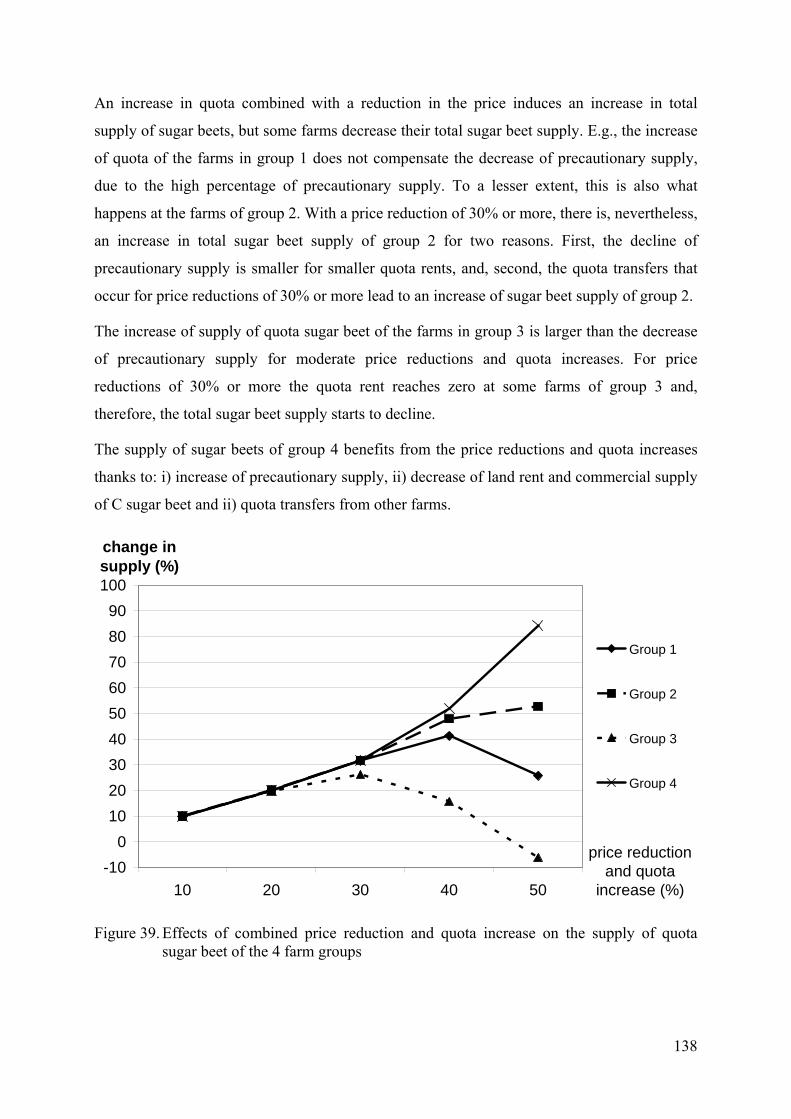
An increase in quota combined with a reduction in the price induces an increase in total

supply of sugar beets, but some farms decrease their total sugar beet supply. E.g., the increase

of quota of the farms in group 1 does not compensate the decrease of precautionary supply,

due to the high percentage of precautionary supply. To a lesser extent, this is also what

happens at the farms of group 2. With a price reduction of 30% or more, there is, nevertheless,

an increase in total sugar beet supply of group 2 for two reasons. First, the decline of

precautionary supply is smaller for smaller quota rents, and, second, the quota transfers that

occur for price reductions of 30% or more lead to an increase of sugar beet supply of group 2.

The increase of supply of quota sugar beet of the farms in group 3 is larger than the decrease

of precautionary supply for moderate price reductions and quota increases. For price

reductions of 30% or more the quota rent reaches zero at some farms of group 3 and,

therefore, the total sugar beet supply starts to decline.

The supply of sugar beets of group 4 benefits from the price reductions and quota increases

thanks to: i) increase of precautionary supply, ii) decrease of land rent and commercial supply

of C sugar beet and ii) quota transfers from other farms.

-100

102030405060708090

100

10 20 30 40 50

price reduction and quota

increase (%)


Group 1

Group 2

Group 3

Group 4

Figure 39. Effects of combined price reduction and quota increase on the supply of quota sugar beet of the 4 farm groups

138

-100

-90

-80

-70

-60

-50

-40

-30

-20

10 20 30 40 50


increase (%)


Group 1

Group 2

Group 3

Group 4

Total

Figure 40. Effects of combined price reduction and quota increase on the supply of C sugar beet of the 4 farm groups

-30

-20

-10

0

10

20

30

40

50

60

10 20 30 40 50


increase (%)


Group 1

Group 2

Group 3

Group 4

Total

Figure 41. Effects of combined price reduction and quota increase on the supply of sugar beet of the 4 farm groups

139

5.3.4 Supply effects of compensation mechanisms Figure 42 and Figure 43 indicate the supply effects of compensating the A sugar beet price

reduction with coupled direct acreage subsidies in case of a 39,5% reduction in the A sugar

beet price as agreed by the European council in November 2005. As expected, a coupled

sugar beet subsidy mitigates the supply effect of the reduction in the price. The coupled

compensation is affected by a modulation of 5%. This means that from the subsidies higher

than 5000 euro, 5% is reduced. The larger farms, mostly situated in group 4, are most affected

by the modulation for high compensation levels. Therefore, for 100% compensation, the

largest decrease of supply of sugar beets is observed in group 4. The farms of groups 1 and 3

are almost not affected by modulation and, for that reason, 100% coupled compensation does

not change their supply behaviour.

A small compensation level gives already a significant increase of sugar beet supply of farms

in group 1, 2 and 3 for two reasons. First, the compensation increases the quota rent, which, in

turn, increases the precautionary C sugar beet supply. Second, supply of quota sugar beet

remains profitable at more farms, resulting in less quota reductions from quota transfers. For

the farms of groups 4 the two effects work oppositely. The precautionary C sugar beet supply

is increased, similar to the farms in other groups, by quota rent increases, but the farms can

obtain fewer additional quota from quota transfers. Fewer quota transfers lead on the one hand

to a lower increase of precautionary C supply but also to a lower supply within the quota.

Therefore, the total sugar beet supply of group 4 even decreases with 20% compensation

compared to no compensation.

There are no quota transfers anymore for higher compensation levels. The differences in

supply behaviour between the groups are, therefore, only induced by differences in

precautionary C sugar beet supply. Group 4 shows a larger reduction in the precautionary

supply than other groups, because the farms of group 4 are more affected by modulation of

the compensations.

The percentage of C sugar beet supply plays a role in the impact of compensation on the total

sugar beet supply. Due to the higher percentage C sugar beet in groups 1 and 2, their total

sugar beet supply reacts more to the coupled compensation than the supply of groups 3 and 4.

140

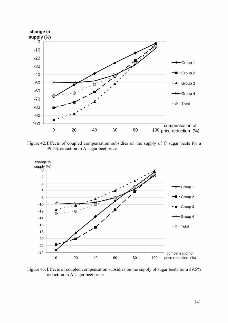
-100

-90

-80

-70

-60

-50

-40

-30

-20

-10

0

0 20 40 60 80 100compensation of

price reduction (%)


Group 1

Group 2

Group 3

Group 4

Total

Figure 42. Effects of coupled compensation subsidies on the supply of C sugar beets for a 39,5% reduction in A sugar beet price

-24

-22

-20

-18

-16

-14

-12

-10

-8

-6

-4

-2

0


price reduction (%)


Group 1

Group 2

Group 3

Group 4

Total

Figure 43. Effects of coupled compensation subsidies on the supply of sugar beets for a 39.5% reduction in A sugar beet price

141

In contrast to the coupled compensation, a decoupled sugar beet subsidy comes as an addition

to the total decoupled subsidies that are granted to the farm according to its eligible area, i.e.,

all land not planted with potatoes and vegetables. The decoupled direct payments have in this

sample of farms no supply inducing effect for sugar beet, because the eligible area is not the

limiting factor for activating decoupled payments. This result corresponds exactly to the

results of Chapter 4.

5.3.5 Income effects of price and quota reductions As in Chapter 4, income effects are measured here as changes in total farm gross margins.

Figure 44 shows the effects of price, Figure 45 the effects of quota reductions and Figure 46

the impact of the combinations of both reductions on the total gross margins of the farm

groups. Because sugar beet is currently an important and the most profitable activity among

these sugar beet farms, the total gross margin is significantly affected. The aggregated total

gross margin declines more sharply as a result of a reduction in price than quota.

The differences in changes in gross margin between farm groups is mainly driven by

differences in quota rent and the share of quota sugar beet in the total crop plan. The farms in

group 3 have the lowest quota rent and their gross margin is, therefore, least affected by the

sugar beet price and quota cuts. Conversely, the farms in group 4 have a very high average

quota rent (25 euro/tonne) and, as a consequence, the decline in the gross margin is higher

than for the farms in group 3.

142

-35

-30

-25

-20

-15

-10

-5

0

-10 -20 -30 -40 -50price

reduction (%)

change in gross margin(%)

Group 1

Group 2

Group 3

Group 4

Total

Figure 44. Effects of reductions in price on the gross margin of the 4 farm groups

-25

-20

-15

-10

-5

0

-10 -20 -30 -40 -50quota

reduction (%)


Group 1

Group 2

Group 3

Group 4

Total

Figure 45. Effects of reductions in quota on the gross margin of the 4 farm groups

143

-40

-35

-30

-25

-20

-15

-10

-5

0



Group 1

Group 2

Group 3

Group 4

Total

Figure 46. Effects of reductions in price and quota on the gross margin of the 4 farm groups

Figure 47 shows the effects on the gross margin of an increase in sugar beet quota combined

with a reduction in the A sugar beet price.

For a moderate price reduction and quota increase, the results look similar to a sole price

reduction. The gross margin decreases more at farms with a high quota rent than at farms with

a lower quota rent.

Price reductions of A sugar beet of 30% or more induce transfers of quota, which provoke a

reduction of the gross margin of farms that can not fill their quota anymore. Mostly farms of

group 4 benefit from the quota transfers and, therefore, their loss of gross margin of a

combined price reduction and quota increase is less severe than their loss of gross margin of a

sole price reduction.

144

-30

-25

-20

-15

-10

-5

0

10 20 30 40 50

price reduction and quota increase

reduction (%)


Group 1

Group 2

Group 3

Group 4

Total

Figure 47. Effects of reductions in price and increase of quota on the gross margin of the 4 farm groups

Figure 48 and Figure 49 show the effects of compensating the A price reduction with coupled

and, respectively, decoupled direct acreage subsidies on the aggregated gross margin of the

simulated FADN sample for a 39,5% reduction in the price. Decoupling the compensation

subsidies mitigates the decline in total gross margin because, for the same amount of

subsidies, sugar beet farms have more flexibility in allocating their activities to maximise

their total gross margins. The difference in gross margin between coupled and decoupled

subsidies is, however, very small. The simulation of the sugar CMO reform, as decided in

November 2005, in our model induces a decline of about 6% in aggregated total gross margin.

145

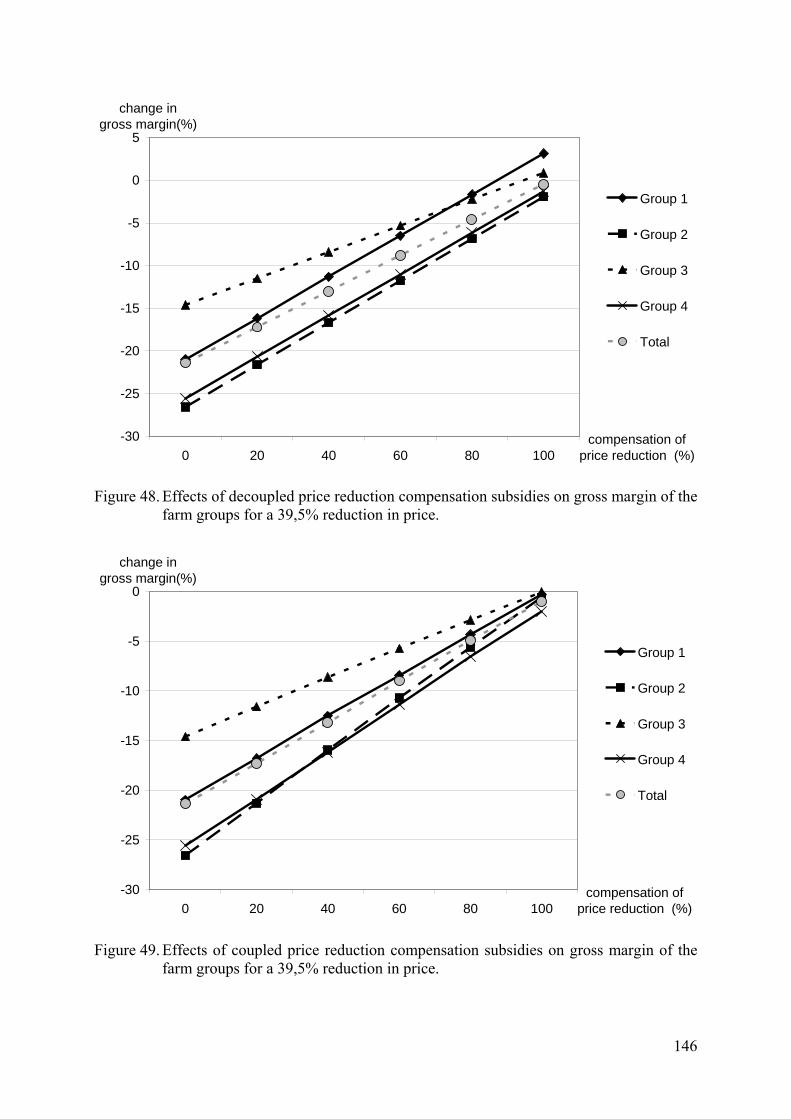
-30

-25

-20

-15

-10

-5

0

5


price reduction (%)


Group 1

Group 2

Group 3

Group 4

Total

Figure 48. Effects of decoupled price reduction compensation subsidies on gross margin of the farm groups for a 39,5% reduction in price.

-30

-25

-20

-15

-10

-5

0


price reduction (%)


Group 1

Group 2

Group 3

Group 4

Total

Figure 49. Effects of coupled price reduction compensation subsidies on gross margin of the farm groups for a 39,5% reduction in price.

146

5.3.6 Supply effects on other crops Table 22 shows to what extent a price reduction compensation, whether coupled or not,

affects the supply of the other major crops of the sugar beet farms in case of a 39,5%

reduction in the price and a 64,2% compensation of the price reduction. Analogous as in

Chapter 4, a price reduction compensation coupled to sugar beet acreage has no additional

influence on the supply of the other crops. In contrast, a price reduction compensation

decoupled of sugar beet acreage increases the supply of the other crops, i.e., mainly cereals,

maize and fallow.


crops of sugar beet farms within the Belgian FADN for a 39,5% reduction in A sugar beet

price Difference (%) Coupled compensation No compensation / Decoupled compensation

Group 1

Group 2

Group 3

Group 4

Total Group 1

Group 2

Group 3

Group 4

Total

Total sugar beet

-8,1 -10,4 -5,4 -7,5 -7,4 -23,3 -21,7 -11,6 -9,5 -12,7

A sugar beet 0,0 0,0 0,0 0,0 0,0 0,3 0,3 -0,6 0,3 0,0

C sugar beet -23,1 -38,3 -46,3 -38,0 -38,7 -67,2 -80,7 -95,3 -49,4 -66,0

Winter cereals

2,8 3,3 3,7 3,3 3,4 6,6 7,7 8,5 7,7 7,9

Summer cereals

0,0 3,0 4,0 3,2 3,4 0,0 7,1 9,2 8,2 8,1

Maize 7,2 0,0 1,7 3,3 2,8 16,8 0,0 4,0 7,6 6,5Wet pulses 0,0 0,0 1,9 1,3 1,4 0,0 0,0 4,5 3,0 3,4

Potatoes 0,6 1,8 0,6 1,3 0,9 1,5 4,2 1,5 3,1 2,2Chicory 0,0 -1,0 -1,9 -3,4 -2,9 -29,8 -35,5 -27,5 -26,7 -27,9Industrial crops

1,5 0,0 0,7 0,0 0,7 3,6 0,0 1,7 0,0 1,7

Other arable crops

0,0 4,5 0,5 0,8 0,7 0,0 10,4 1,1 1,8 1,6

Fallow 0,1 0,1 0,5 3,8 2,1 -0,1 0,0 2,0 9,6 5,3

The results of Table 22 are probably not representative for the total supply of other crops in

Belgium because the sample only consists of farms producing sugar beet. In Belgium cereals,

maize, pulses, potatoes and other crops are also produced at farms without sugar beet, which

are not represented here.

147

5.4 Conclusions

5.4.1 Conclusions with respect to the application Due to the similarities between the EMP and PMP sugar module, the conclusions for the PMP

version that are described in 4.6.1 are also valid here. There are, however, also some

differences in the aggregated results.

The aggregated results are more responsive for the EMP than for the PMP sugar beet module,

due to the flatter estimated cost function and the resulting higher quota rents with the EMP

application. The fact that in the EMP results some farms, for scenarios where the quota rents

increase, become profitable C sugar beet suppliers creates the largest difference with the PMP

results. However, when the sample would be completed with all non-sugar beet farms, there

would be more competition for land and higher land rents. Therefore, profitable C sugar beet

suppliers would than not have been observed.

Chapter 5 provides more details on the differences between farms. This underlines once more

the value of a farm-level approach because the policy makers are not only interested in the

aggregated outcome, but also in the differences for different groups. The details on farm-level

differences give also more insight in the driving factors of the aggregated outcome.

5.4.2 Modelling lessons Chapter 5 resolves two of the problems of the sugar module of SEPALE presented in Chapter

4. Chapter 5 introduces a simultaneous calibration of all sugar beet specific parameters to

avoid the ad hoc assumptions related to the quota rent. At the same time, the number of

parameters in the precautionary supply function is increased resulting in a more flexible

function that should be able to represent the precautionary supply behaviour more

realistically.

As a result, the sugar module of SEPALE can be viewed upon as a real-world example of the

general methodology proposed by Heckelei and Wolff (2003) that we have called EMP in this

dissertation. The differences between the results of the PMP and the EMP approach are rather

small. This confirms partially the sensitivity analysis of the PMP approach. Next subsection

describes these differences, their cause and their consequences. The subsection thereafter tries

to anticipate on the applicability of EMP in other situations.

148

5.4.2.1 Comparison of results of the PMP and EMP sugar beet module of SEPALE

The differences between the results at farm-level are mainly driven by the calibration

approach applied to the sugar module. In the PMP version of the sugar beet module, the sugar

beet parameters depend on the percentage C sugar beet supply, the average costs for sugar

beet, the land price and the calibrated elasticities of other crops. In the EMP version the

parameters are determined by differences in percentage C sugar beet supply, the average costs

for sugar beet and land prices, but during calibration not by different supply elasticities of

other crops. We think, therefore, that the farm-level results of EMP are more reliable, because

the elasticities of other crops are only calibrated in a simplified way and probably prone to

some bias. This bias can influence the PMP results, but not those of EMP.

Another difference between the PMP and the EMP approach is the use of the base data. The

PMP model starts from the percentage C supply from one calibration year, while the

percentage C supply in the EMP version comes from the estimation, which is based on several

years.

5.4.2.2 Applicability of EMP

The results have shown that it is possible to apply EMP to real world situations. There are,

however, some pitfalls that could be avoided here, but that could hamper future applications

in other situations.

Complementary slackness conditions in estimation equations

Section 3.6.2.3 explains the problem, which is also reported by other authors (Gocht, 2005;

Heckelei and Britz, 2005), of complementary slackness equation in an NLP model

formulation.

In the current EMP sugar module of SEPALE, the problem is avoided by making assumptions

on which constraints are binding and which not. However, in certain cases, when the duals of

constraints are close to zero, the modeller is bound by insufficient information to make such

assumptions. In order to increase the applicability of EMP, more research should be done on

the topic of solving MPEC problems.

149

Estimation problems

The structure of an EMP model typically includes also all difficulties that could be

encountered during an estimation process. Because an MP model is not built as the standard

econometric problem with dependent and independent variable, in a lot of cases one can

expect to have a model structure with endogeneity. The complementary slackness constraints

are also in most cases non-linear in parameters and, dependent on the model, the estimator

should also take care of limited dependent variables. Unless the model is simplified, the

modeller may have to program an estimator himself, because standard econometric packages

do not include an estimator that can deal straightforwardly with all these issues in one time.

Complexity of the model

Even though the application of the sugar module has been successful, the rest of the model

still relies on a simplified model that is PMP calibrated. The simultaneous estimation of a

farm-based sector model that includes the sugar module, supply behaviour of other crops and

a module for the animal sector would be much more complicated. If the estimation of such a

model is done step by step, the model has to rely nevertheless on assumptions on the

interaction between the different modules.

This problem is also apparent in the estimation of the sugar module. The results of the

estimation of the sugar parameters depend on the assumption that the approximation of the

shadow cost of land, the land rent, represents the interaction between sugar beet and the other

crops. All other forms of interactions are ignored.

150

General discussion and conclusion20

The dissertation demonstrates how different types (NMP, PMP and EMP) of mathematical

programming models can be applied for farm-level policy analysis. The conclusion discusses

the classification and the definition of the model types followed by a summarising overview

of the applications of the three model types. Next, the conclusion gives some indications of

model type selection. The dissertation finalises with some general concluding remarks and

recommendations for future research.

Definition and classification of the 3 model types

NMP is defined as the type of models in which no algorithm is used or specific steps have

been taken to adjust the model parameters to guarantee that the model precisely reproduces

the observed data. Differently stated, NMP models are MP models without calibration.

According to the definition used in this dissertation, both PMP and EMP rely on calibration.

The difference between both may not always be very clear, because there is still a lot of

discussion on the meaning of calibration and estimation, certainly within the literature of real-

business-cycle economics. Besides the difference in opinion on the meaning of the words,

there is also acrimony on the correctness and utility of different approaches: model calibration

versus model estimation (Quah, 2005). Contemporary economic analysis includes two broad

traditions of fitting models to data. Estimation uses stochastic, theory-based, reduced form

models with few parameters, while calibration of models is done by an extensive collection,

and computation, of consistent fitted values. Although it is widely recognized that both

calibration as estimation fit a model to data and that the exercises are similar, Balistreri and

Hillberry (2005) indicates that the focus of both types of research is different: the calibrators

concentrate on counterfactual simulation while the focus of estimators is on hypothesis

testing.

20 Parts of the general discussion and conclusion have been published as:

Buysse, J., Van Huylenbroeck, G. and Lauwers, L. (2006). Normative, positive and econometric mathematical

programming as tools for incorporation of multifunctionality in agricultural policy modelling. Agriculture,

Ecosystems & Environment, in press.

151

The definition of distinction between PMP and EMP used in this dissertation is as follows.

Both PMP and EMP are useful methodologies for calibration of a cost function at farm level

starting from positive information but, the calibration of PMP is deterministic, while the

calibration of EMP is stochastic. This means that there are zero degrees of freedom in the

PMP calibration equations while there are non-zero degrees of freedom in the EMP

calibration equations. To obtain zero degrees of freedom, the PMP model has either a simple

functional form or it is fed with casual empiricism or knowledge from separate econometric

studies (the definition of calibration according to Hoover, 1995). The EMP calibration with

non-zero degrees of freedom relies on some econometric minimisation algorithm to adjust the

parameters of the model such that the simulated output deviates minimally from the real

output (the definition of calibration according to Kleijnen, 1993).

The classification that we have made between the three types is thus not based on the amount

of econometrics involved in the model. E.g., the NMP application in this dissertation relies on

more estimated functions than the PMP and EMP applications. The classification rather refers

to the way the final step is taken of bringing different model pieces together. We are aware

that the presented typology does not completely correspond to other classifications and that

discussion on the classification could be possible. E.g., Heckelei and Britz (2005) define the

use of phase 1 of a defining character of PMP and call the newly developed approaches

‘alternative approaches to calibration and estimation or programming models’. According to

that definition SEPALE is not a PMP method but belongs to the alternatives, while Paris and

Howitt (1998) is an application of PMP. Howitt (2005) distinguishes PMP (zero degrees of

freedom) and ill-posed ME models (negative degrees of freedom) of which Paris and Howitt

(1998) is an example. The place of the SEPALE applications is not very clear in Howitt’s

classification. The classification in itself is, however, not important. The classification only

facilitates the overview of model types and can support the selection of a model for a specific

research task. More important than the classification, the differences and similarities between

different modelling approaches should become clear.

152

Therefore, a detailed comparison as well as applications of each model type has been

presented. Each application provides us with some experiences with respect to the model type

and can lead to policy recommendations. The policy recommendations of the individual

applications can be interesting, but are not subject of this general conclusion. Instead, the

general conclusion and discussion presents an overview of the strengths and weaknesses of

the three model types. This overview and the experience can be used as hints on model type

selection for future research.

Summarising overview of the applications of the three model types

NMP has been applied for the development of a dairy farm model. The model has shown its

utility for the assessment of the impact of management decisions on the nutrient balance of a

dairy farm. The strength of NMP is this case is the possibility to integrate separately known

functions in one simulation model in order to draw conclusions not only at field or at cow

level, but also at overall farm level. As illustrated, the model can be used to evaluate either

management options at farm level, but also the effect of possible policy options.

The dairy farm application has also illustrated one of the main drawbacks of NMP: the

models’ inability to simulate baseline conditions. The problem of validating this type of

models is to our opinion mainly due to problems of data gathering and influence of external

parameters on the data. This shows at the same time an important advantage of the model:

external parameters influencing observed nutrient balances such as weather conditions and

measurements errors can be eliminated, so that the exact influence of practices and systems

can be evaluated. Or put in a phrase by Hazell and Norton, 1986: “It is after all better to use

good logic (embodied in the model) for policy analysis than to compound the problem of poor

data with poor logic.”

Nevertheless, modellers have devoted more and more time to calibration to avoid the critique

of simulation problems with baseline conditions. This has lead to the development and formal

description of PMP, which has renewed the interest in MP. The main strength of PMP is the

possibility to make use of very few data to model agricultural policies, while being able to

generate plausible results. The plausibility of the results is inherited from the possibility of the

introduction of real-world constraints and of the calibration step.

153

PMP is illustrated in this dissertation with SEPALE. SEPALE consists of a collection of

farm-level PMP models, of which the parameters of the individual farms are calibrated based

on the FADN data. SEPALE is, therefore, an illustration of how PMP can be used with large

farm-level samples. This model makes it possible to account for the individual farm structure

and the interaction between farms. The possibility to simulate the effects according to farm

size or other criteria such as region or farm type also allows to model structural changes of the

sector. SEPALE has been used to simulate the June 2003 CAP reform with varying

decoupling rates and modulation levels and thresholds.

A significant part of the dissertation is devoted to the modelling of quota, the sugar CMO in

particular. The sugar regime forms an interesting challenge for modellers because three

important issues have to be tackled: C sugar beet supply, quota rent approximation and quota

transfers. The most complex element, for sugar beet, is the problem of out-of-quota supply.

Therefore, a precautionary supply function is introduced in the model. The precautionary

supply function describes the increasing C sugar beet supply as a result of increasing quota or

quota rent. In order to make the link with the quota rent during simulation, the programme is

rewritten in its complementary slackness conditions.

The sugar beet application has illustrated the strengths of PMP of generating plausible results

with a rather simply model. However, it has, at the same time, exposed its weaknesses

because calibration of the sugar module and the quota rent approximation have only been

possible with simplifying assumptions. It is certainly true that the plausible results generated

by a PMP model do not guarantee that the response is correct. The limited functional form of

the model and the ad hoc calibration assumptions may influence the results for a great deal

and can introduce subjectivity in the analysis.

To mitigate these problems, time has been invested in the development of an EMP version of

the sugar module. The EMP application has removed the theoretical objections to the ad hoc

calibration assumptions and has also made a more flexible functional form for the

precautionary supply function possible. Nevertheless, the GME estimation is still dependent

on the choice of support points and the choice which parameters should be common for the

sample. These choices can be subject to discussion. In a way, one can, therefore, argue that

EMP does not remove the problems of subjectivity. It is only rearranged into a different

configuration. The main results and conclusions of the EMP and PMP sugar module are also

quite similar. The most important difference is that the quota rent of the EMP application is a

bit higher and the cost functions flatter.

154

A more interesting aspect of the results of the EMP application is the presentation of the

reactions of the different farm groups. Once more, these results highlight the utility of the

farm-level approach. The farm-level approach not only makes it possible to segregate the

results according to farm characteristics. It is also a good instrument to illustrate the economic

mechanisms behind aggregated results and it can simulate structural changes. It should,

however, be emphasized that the farm-level aspect is not limited to EMP. Also NMP and

PMP model can operate at farm-level.

The applications have illustrated the strengths and weaknesses of the MP modelling

approaches. The question is then how to select a model type for a certain research task.

Model type selection

The choice of method depends on three elements: data availability, model focus and research

scope.

Data availability depends on the resources for data collection but also on the type of policy

instruments to model. For a new policy, radically different from the previous, less data are

available and therefore more normative techniques have to be used. Data availability remains

a major prerequisite for applying PMP and EMP. When no empirical data are available, an

MP model will inevitably rely on an NMP technique. In EMP, the combination of

econometrics and programming may help to take full use of the scarce available data.

The model focus can be prescriptive, explorative or descriptive. A model intended for

prescription can only rely on NMP. In a certain sense, the technique can “describe” what

would happen to a reference population when the actors follow the prescribed

recommendations. NMP can also be very useful for demonstration of sensitivity and for

gaining insight in a problem. Therefore, NMP is suited for explorative research of new

opportunities and innovations within a context of resource constraints. PMP and EMP on the

contrary, will be preferred for description and prediction of behaviour and reactions on

modifications in existing policy instruments. These tools are indeed able to take into account

real-observed behaviour (and not a theoretical full adoption of prescriptive recommendations)

and will therefore result in more reliable prediction of consequences of changes in policy

parameters. However, this does not means that PMP and EMP would not allow for

incorporating new policy measures or innovations. These approaches are positive for those

elements that can be integrated in the calibration, but, due to the MP side of the approach,

PMP and EMP can also be normative for those parts where only some basic information about

155

the system (e.g. coming from experimental stations) is available. The main risks for

simulation biases arise, however, when the external introduced normative information

drastically intervenes with the positively calibrated parameters reflecting the unobserved

constraints.

Generally, EMP could be preferred to PMP because, due to the advanced techniques of

descriptive analysis of econometrics, the technique is supposed to be more robust and better at

describing past behaviour. However, the development of an EMP model probably requires

more resources for data collection and for solving the problem numerically.

Finally, the research scope also influences the choice of model. A model only developed for a

specific case can probably attract fewer funds. Therefore, the preferred technique will likely

depend on the time needed for development. In a more general decision support system, with

the possibility of a more or less continuous funding and knowledge exchange organisation,

applicability and robustness will become major criteria for model choice.

The applications in this dissertation have also illustrated the influence of the available time on

the choice of method. When the discussion on the Sugar CMO reform has started,

stakeholders were interested in a quick analysis of the reform proposals, which was first based

on a rather simple PMP model. Later, the PMP variant of the sugar module has been refined

and finally turned into an EMP model. Also the application of SEPALE to simulate the MTR

has shown the influence of the model scope. The transfer of direct payment entitlements was

only a secondary research question and not enough time is yet invested to solve the issue. In a

future research project, where transferring of rights between farms is the focus, specific

algorithms can be development.

Some concluding remarks and recommendations for further research

The dissertation gives a broad overview of the development of MP models and how to select a

model type for a specific research task. However, the overview and the applications do not

deal necessarily with every aspect of the development and simulation.

156

One of the topics that has not been discussed is the sample selection. The PMP and EMP

applications show nevertheless that the sample selection may influence the results

significantly. Arfini et al. (2003) states that the biggest problem common to all the models

solely based on the FADN sample is their representativity with respect to the regional

universe, and the fact that this is strictly linked to the representativity of the FADN sample.

The latter should be guaranteed at regional level for each farm type, but is obviously reduced

when a further subdivision of the farms is made, such as for example, size class. Certainly

when the model uses only a sub-sample of the FADN sample, results may not reflect reality.

To solve the issue of representativity, Arfini et al. (2003) combine the FADN database with

the land use database. This type combination of different databases is interesting aspect for

further research, because it can improve the representativity and increase the availability of

data.

Another issue that deserves more attention in further research is the validation of calibrated

models. One of the important problems with validation of the economic models presented in

this dissertation is the lack of good validation data because the recent CAP reforms with

decoupled payments and strong price reductions of the sugar beet reform are not observed

before. Kleijnen (1999) argues, nevertheless, that validation is possible even if no data are

available. Even if real data are missing, there is still the possibility to do a sensitivity analysis

and to use expert knowledge. If the simulation model’s input/output (I/O) behaviour violates

this qualitative knowledge, the model must be seriously questioned.

Even though this dissertation strongly advocates a farm-level MP modelling approach, many

other valuable approaches exist, with which the described models can be enriched or coupled.

With this respect, current efforts to enrich the model tools with GIS (geo-information

systems), MAS (multi-agents systems), game theoretic heuristics (see e.g. Balman, 1997;

Happe et al., 2004) or with uncertainty in output prices and farmer’s risk aversion (Havlik et

al., 2005) are promising. Another interesting contribution can be expected from institutional

approaches, not only because institutions are part of the system that has to modelled, but also

necessary to improve the policy support organisation. Own experiences strengthen our belief

that human resources prevail on the mere mechanics of modelling. The model tool is not a

jukebox, but needs corporate and evolving knowledge about systems. As a consequence, for

an appropriate organisation of policy impact analysis, it is important to invest in modellers

and not only in models.

157

Finally, another promising research area is the use of models to detect the appropriate objects

for policy impact analysis: what will be the new prototypes of farming systems that may form

the pillars of sustainable agriculture. According to Rossing et al. (1997), these prototypes can

be detected with prospective models taking into account the complex system behaviour. But

also, non-conventional methods, such as participatory techniques where stakeholders

decision makers and modellers closely interact in the problem solving process (see e.g. Buhler

et al., 2002), may be of interest. The main challenge to build this kind of models is to

combine the sparkling ideas picked up in participatory processes with a sound theoretical and

operational model practice.

The dissertation can be concluded with the words of Howitt (2005): “Selection of the best

model for the research task at hand is an art rather than a science. The model builder is

constantly balancing the requirements of realism that complicate the model specification and

solution against the practicality of the model in terms of its data and computational

requirements. There is no ideal model, just some that are more manageable and useful than

others.”

158

References Adenäuer, M., Elouchichi, K., Henry de Frahan, B. and Witzke, H.P. (2004). Impact of

Everything but arms initiative on the EU sugar sub-sector. Selected paper presented at the

International Conference on Policy Modelling, Paris, 30 June – 2 July, 2004.

Adenäuer, M., Heckelei, T. (2005). Economic incentives to supply sugar beet in Europe. In:

Arfini, F. (Ed.) Modelling agricultural policies: state of the arte and new challenges. Monte

Universita Parma, Parma, p. 588-609.

Asijee, K. (1993). Handboek voor de rundveehouderij, publicatie nr. 35, Informatie en Kennis

Centrum Rundveehouderij, Lelystad, 629 p.

Arfini, F., Donati, M. and Paris, Q. (2003). A National PMP Model for Policy Evaluation in

Agriculture Using Micro Data and Administrative Information. Contributed paper to

International Conference: Agricultural policy reform and the WTO: where are we heading?

Capri (Italy), June 23-26, 2003.

Arfini, F. (2001). Mathematical programming models employed in the analysis of the

common agricultural policy. INEA Working Paper n.9.

Arriaza, M. and Gómez-Limón, J.A. (2003). Comparative performance of selected

mathematical programming models. Agricultural Systems, 77(2): 155-171.

Arndt, C., Robinson, S. and Tarp, F. (2002). Parameter estimation for a computable general

equilibrium model: a maximum entropynext term approach. Economic Modelling, 19(3): 375-

398.

Balistreri, E.J. and Hillberry, R.H. (2005). Estibration: An Illustration of Structural Estimation

As Calibration. Working paper. http://www.mines.edu/~ebalistr/Papers/estibration.pdf

Behaeghe, T. (1979). Seizoensvariatie in de grasgroei, Proefschrift tot het verkrijgen van de

graad van geaggregeerde voor het hoger onderwijs, RUG, Gent, 272 p.

Bondt, N., Jansen, L.F. and Hoste, R. (2001). Economie en welzijn op melkveebedrijven: een

verkennend onderzoek. LEI, Den Haag.

Brent, R.P. (1973). Algorithmes for minimization without derivatives. Prentice Hall,

Engelwood Cliffs, New Jersey.

159

Britz W., Heckelei, T. and Wolff, H. (2003). Symmetric Positive Equilibrium Problem: A

Framework for rationalizing Economic Behavior with Limited Information: Comment.

American Journal of Agricultural Economics, 85(4): 1078-81.

Brown, P.J. and Oman, S.D. (1991). Double points in nonlinear calibration. Biometrika, 78:

33-43.

Buhler, W., Morse, S., Arthur, E., Bolton, S. and Mann, J. (2002). Science, agriculture and

research, a compromised participation? Earthscan Publications Ltd, London.

Bureau, J.C., Guyomard, H. and Requillart, V. (2001). On Inefficiencies in the European

Sugar Sector. Journal of Policy Modeling, 23(6): 659-667.

Bureau, J.C., Guyomard, H., Morin, L. and Réquillard, V. (1997). Quota Mobility in the

European Sugar Regime. European Review of Agricultural Economics, 24: 1-30.


Huylenbroeck, G. and Van Meensel, J. (2004). Modelling the impact of sugar reform on

Belgian Agriculture. Selected paper presented at the International Conference on Policy

Modelling, Paris, 30 June - 2 July, 2004.


Huylenbroeck, G. and Van Meensel, J. (2005a). Quota in Agricultural Positive Mathematical

Programming Models. In: Arfini, F. (Ed.) Modelling agricultural policies: state of the arte and

new challenges. Monte Universita Parma, Parma, p. 233-251.

Buysse, J., Van Huylenbroeck, G. and Lauwers, L. (2006). Normative, positive and

econometric mathematical programming as tools for incorporation of multifunctionality in

agricultural policy modelling. Agriculture, Ecosystems & Environment, in press.

Buysse, J., Van Huylenbroeck, G., Vanslembrouck, I. and Vanrolleghem, P. (2005b).

Simulating the influence of management decisions on the nutrient balance of dairy farms.

Agricultural Systems, 86: 333-348.

Chambers, R. G. (1988). Applied Production Analysis: A Dual Approach. Cambridge

University Press.

Coléno, F.C. and Duru, M. (1999). A model to find and test decision rules for turnout date and

grazing area allocation for a dairy cow system in spring. Agricultural Systems, 61: 151-164.

160

Commission of the European Communities. (1999). The CAP reform – A policy for the

future.

Commission of the European Communities. (2002). Implementation of Council Directive

91/676/EEC concerning the protection of waters against pollution caused by nitrates from

agricultural sources.

Commission of the European Communities. (2003a). Accomplishing a sustainable agricultural

model for Europe through the reformed CAP – the tobacco, olive oil, cotton and sugar sectors.

Commission of the European Communities. (2003b). Reforming the European Union’s sugar

policy, Summary of impact assessment work. Commission Staff Working Paper, SEC(2003)

1022, Brussels.

Commission of the European Communities. (2004a). Accomplishing a sustainable agricultural

model for Europe through the reformed CAP - sugar sector reform. Communication from the

Commission to the Council and the European parliament, COM (2004) 499 final, Brussels.

Commission of the European Communities. (2004b). Common Organisation of the Sugar

Market-Description. Brussels:

http://europa.eu.int/comm/agriculture/markets/sugar/reports/descri_en.pdf (27.12.03).

Commission of the European Communities. (2005). Proposal for a Council Regulation on the

common organisation of the markets in the sugar sector. SEC (2005) 808, Brussels.

Communication from the Commission to the Council and the European parliament, COM

(2003) 554 final, Brussels.

CVB. (1996). Voedernormen landbouwhuisdieren en voederwaarde veevoeders. Centraal

veevoederbureau, Lelystad.

Dawkins, C., Srinivasan, T.N. and Whalley, J. (2001). Calibration. In: Heckman, J.J. and

Leamer, E.E. Handbook of Econometrics, vol. 5, chapter 58, Elsevier, Amsterdam.

Den Boer, D.J. (1999). Management als kans om de N – benutting in de melkveehouderij te

verbeteren. In: Samenvatting symposium Nutriënten Management 1999. Nutriënten

Management Instituut, Wageningen.

Deuninck, J., Dhont, S. and Viaene, J. (2001). Structurele Aanpassingen voor de Vlaamse

Varkenshouderij. Universiteit Gent, Gent.

161

Drud, A. (2004). CONOPT documentation. ARKI Consulting and Development A/S,

Bagsvaerd, Denmark.

Fernagut, B., Nasse, L., Lauwers, L., Buysse, J., Van Huylenbroeck, G., Harmingie, O.,

Polomé, P. and Henry de Frahan, B. (2004). Organisation of knowledge transfer in

agricultural policy analysis. In: Van Huylenbroeck, G., Verbeke, W. and Lauwers, L. (Eds),

Role of institutions in rural policies and agricultural markets. Elsevier B.V., Amsterdam, p.

183-196.

Frandsen, S.E., Jensen, H.G., Yu, W. and Walter-Jorgensen, A. (2003). Reform of EU sugar

policy: price cuts versus quota reductions. European Review of Agricultural Economics, 30:

1-26.

Fraser, I., McInnes, A. and Russel, N. (1997). The allocation of sugarbeet production

contracts: an application of calibrated production equilibrium modelling. Journal of

Agricultural Economics, 48(2): 139-150.

Gocht, A. (2005). Assessment of simulation behaviour in different mathematical

programming approaches. In: Arfini, F. Modelling agricultural policies: state of the arte and

new challenges. Monte Universita Parma, Parma, p. 166-188.

Gohin, A. and Bureau, J.C. (2006). Modelling the EU sugar supply to assess sectoral policy

reforms. European Review of Agricultural Economics, 33(2): 223-247.

Golan, A., Judge, G. and Miller, D. (1996). Maximum Entropy Econometrics. Wiley,

Chichester, UK.

Gomez-Limon, J.A., Arriaza, M. and Berbel, J. (2002). Conflicting implementation of

agricultural and water policies in irrigated areas in the EU. Journal of Agricultural Economics,

53: 259-281.

Gomez-Limon, J.A. and Riesgo, L. (2004). Irrigation water pricing: differential impacts on

irrigated farms. Agricultural Economics, 31: 47-66

Graindorge C., Henry de Frahan, B. and Howitt, R. (2001). Analysing the Effects of Agenda

2000 Using a CES Calibrated Model of Belgian Agriculture. In: Heckelei, T., Witzke, H.P.

and Henrichsmeyer, W. (Eds.) Agricultural Sector Modelling and Policy Information

Systems, Vauk Verlag, Kiel..

162

Happe, K., Balmann, A. and Kellerman, K. (2004). An agent-based analysis of different direct

payment schemes for the German region Hohenlohe. In: Van Huylenbroeck, G., Verbeke, W.

and Lauwers, L. (Eds). Role of institutions in rural policies and agricultural markets. Elsevier

B.V., Amsterdam, p. 171-182.

Havlik, P., Veysset, P., Boisson J-M., Lherm, M. and Jacquet, F. (2005). Joint production

under uncertainty and multifunctionality of agriculture: policy considerations and applied

analysis. European Review of Agricultural Economics, 32: 489-515.

Hazell, P.B.R. and Norton, R.D. (1986). Mathematical programming for economic analysis in

agriculture. Macmillan Publisher Company, New York.

Heckelei, T. (2002). Calibration and estimation of programming models for agricultural

supply analysis, Habilitationsschrift, Bonn.

Heckelei, T. and Britz, W. (2000). Positive mathematical programming with multiple data

points: a cross-sectional estimation procedure. Cahiers d'Economie et Sociologie Rurales, 57:

28-50.

Heckelei, T. and Britz, W. (2001). Concept and Explorative Application of an EU-wide,

Regional Agricultural Sector Model. In Heckelei, T., Witzke, H.P. and Henrichsmeyer, W.

(Eds.) Agricultural Sector Modelling and Policy Information Systems, Vauk Verlag, Kiel.

Heckelei, T. and Britz, W. (2005). Models based on positive mathematical programming:

state of the art and further extentions. In: Arfini, F. (Ed.). Modelling agricultural policies:

state of the arte and new challenges. Monte Universita Parma, Parma, p. 48-74.

Heckelei, T. and Wolff, H. (2003). Estimation of constrained optimisation models for

agricultural supply analysis based on generalised maximum entropy. European Review of

Agricultural Economics, 30(1): 27-50.

Helming, J.F.M., Peeters, L. and Veendendaal. P.J.J. (2001). Assessing the Consequences of

Environmental Policy Scenarios in Flemish Agriculture. In Heckelei, T., Witzke, H.P. and

Henrichsmeyer, W. (Eds.) Agricultural Sector Modelling and Policy Information Systems,

Vauk Verlag, Kiel.

163


Huylenbroeck, G. and Van Meensel, J. (2006). Positive mathematical programming for


Bjorndal T., Epstein, R. and Romero, C. (Eds.). Management of Natural Resources: A




Herrero, M., Fawcett, R.H. and Dent, J.B. (1999). Bio-economic evaluation of dairy farm

management scenarios using integrated simulation and multiple-criteria models. Agricultural

Systems, 62: 169-188.

Hoover, K.D. (1995). Facts and artifacts: calibration and the empirical assessment of real-

business-cycle models. Oxford economic papers, 47(1): 24-44.

Howitt, R E. (1995a). Positive Mathematical Programming. American Journal of Agricultural

Economics, 77(2): 329-342.

Howitt, R.E. (1995b). A Calibration Method for Agricultural Economic Production Models,

Journal of Agricultural Economics, 46(2): 147-159.

Howitt, R.E. (2005). Agricultural and Environmental Policy Models: Calibration, Estimation

and Optimization. UCDavis, California.

Jarrige, R. (1988). Alimentation des bovins, ovins et caprins. INRA, Parijs.

Jarvis, S.C., Wilkins, R.J. and Pain, B.F. (1996). Opportunities for reducing the

environmental impact of dairy farming managements: a systems approach. Grass and Forage

Science, 51: 21-31.

Judez, L., Chaya, C., Martinez, S. and Gonsalez, A.A. (2001). Effects of the measures

envisaged in 'Agenda 2000' on arable crop producers and beef and veal producers: an

application of Positive Mathematical Programming to representative farms of a Spanish

region. Agricultural Systems, 67: 121-138.

Kleijnen, J.P.C. (1993). Verification and validation of simulation models. Mimeo, Tilburg

University.

Kleijnen, J.P.C. (1999). Validation of models: statistical techniques and data availability. In:

Farrington, P.A., Nembhard, H.B., Sturrock, D.T. and Evans, G.W. (Eds.). Proceedings of the

1999 Winter Simulation Conference.

164

Korver, S., Van Arendonk, J.A.M. and Koops, W.J. (1985). A function for live-weight change

between two calvings in dairy cattle. Animal production, 40: 233-241.

Kuipers, A., Mandersloot, F. and Zom, R.L.G. (1999). An approach to nutrient management

on dairy farms. Journal of Dairy Science. 82, suppl. 2: 84-89.

Lewis, D.R., McGechan, M.B. and McTaggart, I.P. (2002). Simulating field-scale nitrogen

management scenarios involving fertiliser and slurry applications. Agricultural Systems, 73:

1-22.

Mahler, P. (1994). Efficiency losses as a result of insufficient structural adjustments due to the

EC sugar regime: the case of Germany. European Review of Agricultural Economics, 21:

199-218.

McCarl, B.A. and Spreen, T.H. (2004). Applied Mathematical Programming using Algebraic

Systems. College Station, TX: Department of Agricultural Economics, Texas A&M

University.

Michiels, J. Carlier, L. and Verbruggen, I. (1998). Mineralenbalansen en hun gebruik op

melkveebedrijven. In: Van Huylenbroeck, G. and Jacobs, G. Naar een duurzame grasland en

groenvoederuitbating. Ministerie van landbouw, Brussel, p. 27-49.

Mills, G. (1984). Optimisation in economic analysis. George Allen & Uwin Ltd, London, UK,

193 p.

Moro, D. and Sckokai, P. (1999). Modelling the CAP arable crop regime in Italy: degree of

decoupling and impact of Agenda 2000. Cahiers d'Economie et Sociologie Rurales, 53: 50-73.

Mulier, A., Hofman, G., Baecke, E., Carlier, L., De Brabander, D., De Groote, G., De Wilde,

R., Fiems, L., Janssens, G., Van Cleemput, O., Van Herck, A., Van Huylenbroeck, G. and

Verbruggen, I. (2003). A methodology for the calculation of farm level nitrogen and

phosphorous balances in Flemish agriculture. European Journal of Agronomy, 20: 45-51.

Nevens, F. and Reheul, D. (1998). Gebruik van toegediende stikstof door grasland en

groenvoedergewassen. In: Van Huylenbroeck, G. and Jacobs, G., Naar een duurzame grasland

en groenvoederuitbating. Ministerie van landbouw, Brussel, p. 85-108.

O’Toole, R. and Matthews, A. (2002). General Equilibrium, Partial Equilibrium and the

Partial Derivative: Elasticities in a CGE model. Paper presented to the International

Conference on Global Modeling, EcoMod2002, Brussels, 4-6 July.

165

Overvest, J. and Laeven-kloosterman, A.F. (1984). Grasland-gebruikssystemen op het

gezinsbedrijf. Praktijkonderzoek veehouderij, Wageningen.

Pagan, A. (1994). Introduction calibration and econometric research: an overview. Journal of

Applied Econometrics, 9: s1-s10.

Pannell, D.J., 1997. Sensitivity analysis of normative economic models: theoretical

framework and practical strategies. Agr. Econ. 16, 139-152.

Paris, Q. (1997). CAPRI Meeting Follow-up, CAPRI Workshop in Reggio Emilia, Italy, May

1997.

Paris, Q. (2001). Symmetric Positive Equilibrium Problem: A framework for rationalizing

economic behavior with limited information, American Journal of Agricultural Economics,

83(4): 1049-1061.

Paris, Q. and Arfini, F. (2000). Frontier Cost Functions, Self-Selection, Price Risk, PMP and

Agenda 2000, Eurotools Working Papers Series, No. 20, May 2000.

Paris, Q. and Howitt, R.E. (1998). An analysis of ill-posed production problems using

Maximum Entropy. American Journal of Agricultural Economics, 80(1): 124-138.

Paris, Q. and Howitt, R.E. (2001). The Multi-Output and Multi-Input Symmetric Positive

Equilibrium Problem. In Heckelei, T., Witzke, H.P. and Henrichsmeyer, W. (Eds.).

Agricultural Sector Modelling and Policy Information Systems, Vauk Verlag, Kiel.

Pau Vall, M. and Vidal, C. (1999). Nitrogen in agriculture. In: European Commission,

Agriculture, environment, rural development, facts and figures. A challenge for agriculture.

European Communities, Luxembourg, p. 167-180.

Preckel, P. V., Harrington, D. and Dubman, R. (2002). Primal/dual positive math

programming: illustrated through an evaluation of the impacts of market resistance to

genetically modified grains. American Journal of Agricultural Economics, 84(3): 679-690.

Quah, D.T. (1995). Business cycle empirics: calibration and estimation. The Economic

Journal, 105: 1594-1596.

Ramsden, S., Gibbons, J. and Wilson, P. (1999). Impacts of changing relative prices on farm

level dairy production in the UK. Agricultural Systems, 65: 201-215.

166

Robinson, S., Burfisher, M., McDonald, S. and Thierfelder, K. (2006). Deep Integration and

Trade Productivity Links:Tentative Lessons for CGE International Trade Models. Paper for

presentation at the GTAP Annual Conference, Addis Ababa, Ethiopia.

Röhm, O. and Dabbert, S. (2003). Integrating Agri-Environmental Programs into Regional

Production Models: An extension of positive mathematical programming. American Journal

of Agricultural Economics, 85(1): 254-65.

Romero, C. and Rehman, T. (1989). Multiple criteria analysis for agricultural decisions.

Developments in agricultural economics. Elsevier B.V., Amsterdam.

Rossing, W. A. H., Meynard, J. M. and van Ittersum, M. K. (1997). Model-based explorations

to support development of sustainable farming systems: case studies from France and the

Netherlands. European Journal of Agronomy, 7: 271-283.

Salvatici, L., Anania, G., Arfini, F., Conforti, P., De Muro, P., Londero, P. and Sckokai, P.

(2000). Recent developments in modelling the CAP: hype or hope? Plenary paper on 65th

EAAE Seminar, Bonn (Germany), March, 29-31.

Schils, R.L.M. and Snijders P.J.M. (1988). Stikstofwerking van runderdrijfmest op grasland.

Publicatie nr. 60, PR Lelystad.

Schreuder, R., van Middelkoop, J.C., Aalenhuis, J., Mandersloot., F., 1995. Mineralenstroom

milieumodule in BBPR. Praktijkonderzoek veehouderij, Wageningen.

Tamminga, S. (1992). Nutrition management of dairy cows as a contribution to pollution

control. Journal of Dairy Science, 75: 345-357.

Thornley, J.H.M. and Johnson, I.R. (1990). Plant and crop modelling. Oxford Science

Publications.

Thornton, P.K. and Herrero, M. (2001). Integrated crop–livestock simulation models for

scenario analysis and impact assessment. Agricultural Systems. 70, 581-602.

Treaty of Rome. (1957). Treaty establishing the European Economic Community.

Van Arendonk, J.A.M. (1985). A model to estimate the performance, revenues and costs of

dairy cows under different production and price situations. Agricultural Systems, 16: 157-189.

Van Bruchem, J., Verhoeven, F., Brussaard, L., Tamminga, S. (1999). Diet and manure

characteristics in relation to nitrogen flows in a dairy farming system. In: D. van der Heide et

al. (Eds.). Regulation of feed intake. CAB International.

167

van Calker, K.J., Berentsen, P.B.M., de Boer, I.M.J., Giesen, G.W.J. and Huirne, R.B.M.,

(2004). An LP-model to analyse economic and ecological sustainability on Dutch dairy farms:

model presentation and application for experimental farm "de Marke". Agricultural Systems,

82: 139-160.

Van der Schans, F.C. (2000). Koeien binnen of buiten? Afwegingen bij het weiden van

melkvee. Centrum voor Landbouw en Milieu, Utrecht.

Van Huylenbroeck, G., Jacobs, G. and Vanrolleghem, P. (2000). A simulation model to

evaluate the impact of environmental programmes on dairy farms. International transactions

in operational research., 7: 171-183.

Verbruggen, I. (2000). Graslandopbrengsten. 5b land- en tuinbouw Meetjesland, 5(2): 8-9.

Vermeltfoort, J., Breembroek, J., Muller, B., Van Dijk, H., Beldman, A. and Ondersteijn, C.

(2001). Analyse melkveebedrijven. Project praktijkcijfers 2, Houten.

Witzke, H.P. and Kuhn, A. (2003). Assessing Reform Options for the Sugar Common Market

Organisation - Quantitative Analyses with Interlinked Models. Paper presented in Stuttgart-

Hohenheim.

Wood, P.D.P. (1967). Algebraic model of the lactation curve in dairy cattle. Nature, 216: 164-

165.

Wood, P.D.P. (1977). The biometry of lactation. Journal of agricultural science, 88: 333-339.

168

Summary The growing interest in policy support oriented research in agriculture originates from the

need for policy makers of making quickly good decisions in complex situations. The

dissertation focuses on some recent developments of farm-level mathematical programming

models as one type of quantitative models that can be used as a tool for agricultural policy

support. Mathematical programming (MP) has become an important and widely used tool for

analysis in agriculture and economics, because MP models offer unique advantages over other

methods of agricultural sector analysis being able to address the multivariant and highly

interlinked nature of agriculture (Hazell and Norton, 1986).

The dissertation distinguishes three main types of MP models. The first type of models that is

developed and often applied belongs to the normative mathematical programming (NMP)

approach. During the 90’s positive mathematical programming (PMP) has become an

important tool for policy analysis. More recently, the attempt to combine econometrics and

mathematical programming models leads to a new field of empirical investigation, what we

would like to name econometric mathematical programming (EMP).

In the NMP models parameters of the objective function and constraints are not calibrated.

NMP models do not require base data and, therefore, sufficient knowledge of the system

allows the construction of an NMP model. As a consequence, NMP does not guarantee to

reproduce the observed or baseline data.

In PMP models, on the other hand, some parameters are adjusted to reproduce exactly a

baseline. Because this type of models is based on empirical data the method is called positive.

The main purpose of this descriptive type of models is to explain producer’s reactions to

external changes. PMP models are therefore above all interesting for policy makers.

169

While in PMP models the calibration relies mainly on direct assignment rules, a new type of

MP, EMP, can be distinguished where the calibration process is the result of an estimation

procedure (proposed by Heckelei and Wolff, 2003). EMP is an attempt to combine the best of

worlds: econometrics and programming models. EMP models benefit from the advanced

techniques in descriptive analysis of econometrics while being able to introduce changes in

the underlying economic structure through the mathematical programming side of the

approach. These changes in economic structure have been increasingly important in

agricultural policy analysis, for example, due to the recent policy developments of price

support to coupled direct payments and finally to decoupled direct payments. Also other

policy instruments such as production quota, cross compliance elements, fallow restrictions

and environmental constraints are quite easy to introduce in a programming model.

The combination of econometrics and programming models is certainly not new. In order to

obtain more realistic simulation behaviour, the objective function or the constraints are often

supplemented by external estimated functions or parameters. This can, however, introduce

however difficulties or even inconsistencies (Heckelei, 2002). The most obvious example of

such inconsistencies is the use of external estimated supply elasticities to build a supply

function in a programming model. If this supply function is combined with other constraints

in one programming model, the simulation results will not reproduce the original external

estimated supply elasticities. There exist approaches for getting round this problem (Heckelei,

2002), but it is often more useful to apply directly EMP.

EMP is based on the idea of using the set of first-order optimality conditions of the final

simulation model as estimation equations. The parameter estimates will be in line with the

simulation model and, therefore, inconsistencies are avoided.

The objectives of this dissertation are to describe these three types of MP models in detail, to

develop tools for agricultural policy support based on the three types of MP and to apply the

developed tools on specific cases. The applications should prove the utility of the models for

policy analysis and can lead to policy recommendations, but these recommendations

themselves do not form topics for the main conclusions of the dissertation. Instead, the

strengths and weaknesses of the different models are reviewed and compared according to the

dimensions of the applications such as the purpose of the model and the intended users. The

model reviews lead to recommendations for the selection of methods for a research task at

hand. The choice of method depends mainly on data availability and model focus.

170

For a new policy, radically different from the previous, less data are available and therefore

more normative techniques have to be used. Data availability remains a major prerequisite for

applying PMP and EMP. When no empirical data are available, an MP model will inevitably

rely on an NMP technique. In EMP, the combination of econometrics and programming may

help to take full use of the scarce available data.

The model focus can be prescriptive, explorative or descriptive. A model intended for

prescription can only rely on NMP. NMP can also be very useful for demonstration of

sensitivity and for gaining insight in a problem. Therefore, NMP is suited for explorative

research of new opportunities and innovations within a context of resource constraints. PMP

and EMP on the contrary, will be preferred for description and prediction of behaviour and

reactions on modifications in existing policy instruments.

Generally, EMP should be more robust and theoretically correct than PMP due to the

advanced techniques of descriptive analysis of econometrics. However, the application of

EMP has shown that the development of an EMP model requires more resources for data

collection and for numerical solving the problem. Currently, EMP is only applied yet to

problems with a limited size and complexity.

171

Samenvatting De stijgende interesse in beslissingsondersteunend onderzoek in de landbouw vloeit voort uit

de behoefte van beleidsmakers om snel goede besluiten te nemen in complexe situaties. Deze

verhandeling behandelt een aantal recente ontwikkelingen van bedrijfsspecifieke

mathematische programmeringsmodellen als één type van kwantitatieve beleidsonder-

steunende modellen. Mathematische programmering (MP) is een belangrijk en veel gebruikt

hulpmiddel voor analyse in landbouw en economie geworden omdat het unieke voordelen

biedt t.o.v. andere methodes door de mogelijkheid om de complexe interacties relatief

eenvoudig te beschrijven (Hazell en Norton, 1986).

Deze verhandeling onderscheidt drie belangrijke types van MP modellen. De eerste

ontwikkelde MP modellen behoren tot het type van Normatieve MP (NMP) modellen. Tijdens

de jaren '90 is Positieve MP (PMP) een belangrijk hulpmiddel voor beleidsanalyse geworden.

Recentelijk, heeft de combinatie van econometrie en MP geleid tot een nieuw domein van

empirisch onderzoek, in deze verhandeling econometrische MP (EMP) genoemd.

In NMP worden de parameters van het model niet geijkt. De ontwikkeling van NMP modellen

vereist daarom geen empirische gegevens. Voldoende kennis van het systeem volstaat voor de

bouw van een NMP model. NMP garandeert daardoor echter niet dat een referentiesituatie

kan gereproduceerd worden.

PMP modellen gebruiken ijking om bepaalde parameters aan te passen zodat een

referentiesituatie precies wordt gereproduceerd. Het belangrijkste doel van dit type van

modellen is de beschrijving van reacties van landbouwers op externe veranderingen. PMP

modellen zijn daarom in de eerste plaats interessant voor beleidsanalyse.

In tegenstelling tot PMP, waar de ijking gebaseerd is op vergelijkingen zonder

vrijheidsgraden, wordt in EMP geijkt met een schattingsprocedure. EMP is een poging om het

beste van econometrie en MP te combineren. EMP benut de voordelen van de geavanceerde

technieken in beschrijvende analyse van econometrie terwijl ook veranderingen in de

onderliggende economische structuur in het model kunnen gebracht worden via MP. Deze

veranderingen in economische structuur worden steeds belangrijker in landbouwbeleids-

analyse omwille van de recente nieuwe beleidsinstrumenten die steun loskoppelen van

productie. Ook andere beleidsinstrumenten zoals productiequota, randvoorwaarden (cross-

compliance), braakverplichtingen en milieubeperkingen zijn gemakkelijker in een MP model

te introduceren dan in andere types van modellen.

172

De combinatie van econometrie en MP is zeker niet nieuw. Om realistischer simulatiegedrag

te verkrijgen, worden de objectieffunctie of de beperkingen vaak aangevuld door externe

geschatte functies of parameters. Dit kan echter moeilijkheden of zelfs inconsistenties

introduceren (Heckelei, 2002). Het duidelijkste voorbeeld van dergelijke inconsistentie is het

gebruik van extern geschatte aanbodselasticiteiten om de parameters van een aanbodsfunctie

in een MP model te kwantificeren. Door de combinatie van de aanbodsfunctie met

bijkomende beperkingen in een MP model, zullen de simulatieresultaten niet de originele

extern geschatte aanbodselasticiteit reproduceren. Hoewel het mogelijk is om dit probleem te

omzeilen (Heckelei, 2002), is het toch nuttiger om rechtstreeks EMP toe te passen. EMP is

gebaseerd op het gebruik van de optimaliteitscondities van het MP model als

basisvergelijking voor de schattingsprocedure. Het model met de geschatte parameters

reproduceert daarom altijd de geobserveerde gegevens en inconsistenties worden vermeden.

De doelstellingen van deze verhandeling is het beschrijven en toepassen van deze drie types

van MP modellen. De toepassingen illustreren het nut van de modellen voor beleidsanalyse en

kunnen tot beleidsaanbevelingen leiden. Deze aanbevelingen vormen geen onderwerp voor de

eindconclusies van de verhandeling.

In plaats daarvan, worden de sterke punten en de zwakheden van de verschillende modellen

vergeleken. Dit overzicht moet leiden tot aanbevelingen voor de selectie van de juiste

methode voor een specifieke onderzoeksopdracht. De keuze van methode hangt hierbij

hoofdzakelijk af van gegevensbeschikbaarheid en de focus van het model.

Voor een nieuw beleid, sterk verschillend van het vorige, zijn uiteraard minder gegevens

beschikbaar en daarom moeten meer normatieve technieken worden gebruikt. De

beschikbaarheid van gegevens blijft immers een belangrijke eerste vereiste voor het toepassen

van PMP en EMP. Wanneer geen empirische gegevens beschikbaar zijn, zal MP zich

onvermijdelijk op een NMP techniek moeten baseren. In EMP, kan de combinatie van

econometrie en MP bijdragen tot een optimale benutting van de beperkte gegevens.

173

Ook de focus van het onderzoek - prescriptief, verkennend of beschrijvend - bepaalt mee welk

type model het meest in aanmerking komt. Een prescriptief model kan enkel via NMP. Ook

voor verkennend onderzoek kan NMP zeer nuttig zijn bij het creëren van inzicht in een

probleem en het onderzoeken van nieuwe kansen en innovaties binnen een context van

beperkte middelen. PMP en EMP zullen echter meer verkozen worden voor de beschrijving

en voorspelling van gedrag en reacties op wijzigende externe omstandigheden. Over het

algemeen zou EMP robuuster en theoretisch correcter moeten zijn dan PMP dankzij de

geavanceerde technieken van beschrijvende analyse van econometrie. De EMP toepassing

heeft nochtans aangetoond dat de ontwikkeling van een EMP model meer middelen voor

gegevensinzameling en voor het numeriek oplossen het probleem vereist. Momenteel, kan

EMP daarom enkel toegepast worden op problemen met een beperkte grootte en complexiteit.

174

Scientific curriculum vitae

Jeroen Buysse was born in Eeklo on June 3, 1978 and has followed secondary eductation at

the Sint-Vincentiuscollege in Eeklo. In 2001, he has received the degree of Bio-engineer in

Agricultural Sciences at Universiteit Gent. In 2006, he has also successfully finished to

doctoral training program.

In August 2001 he has started as scientific researcher at the department of Agricultural

Economics, Faculty of Bioscience engineering, Universiteit Gent. First, from August 2001 to

February 2002, he has worked on a bio-economic simulationproject of Flemisch dairy farms

in collaboration with the Department of Applied Mathematics, Biometrics and Process

Control. From February 2002 to May 2006, he has collaborated in the SEPALE project

(System for Evaluation of Agro- and Agro-environmental Policies) together with CLE and

UCL. From October 2005 to October 2006 he has also been involved in a project to develop a

model for waste management.

Journal papers

Buysse, J., Van Huylenbroeck, G., Vanslembrouck, I. and Vanrolleghem, P. (2005).

Simulating the influence of management decisions on the nutrient balance of dairy farms,

Agricultural Systems, 86(2), p. 333-348.

Buysse, J. Van Huylenbroeck, G. and Ludwig Lauwers. Normative, positive and econometric

mathematical programming as tools for incorporation of multifunctionality in agricultural

policy modelling. Agriculture, Ecosystems & Environment, in press.

Henry de Frahan, B., Elouhichi, K., Harmignie, O., Polomé, P., Van Huylenbroeck, G.,

Buysse, J., Lauwers, L. and Fernagut, B. (2004). La PAC : Une analyse de la réforme récente.

Regards Economique, 19, 2-13.

175

Chapters in books or proceedings


Huylenbroeck, G. and Van Meensel, J., (2005). Quota in Agricultural Positive Mathematical

Programming Models. In: Arfini, F. (2005). Modelling agricultural policies: state of the arte

and new challenges. Monte Universita Parma, Parma, pp. 233-251.

Fernagut, B., Nasse, L., Lauwers, L., Buysse, J., Van Huylenbroeck, G., Harmingie, O.,

Polomé, P. and Henry de Frahan, B. (2004). Organisation of knowledge transfer in

agricultural policy analysis. In: Van Huylenbroeck, G., Verbeke, W. and Lauwers, L. (eds),

Role of institutions in rural policies and agricultural markets, Amsterdam, Elsevier B.V., 183-

196.

Fernagut, B., Gabriëls, P., Lauwers, L., Van Meensel, J., Buysse, J., Van Huylenbroek, G.,

Harmignie, O., Polomé, P. and Henry de Frahan, B. (2004). Mogelijke gevolgen van de

suikerhervorming voor de bietenplanters. Brussel, Centrum voor Landbouweconomie, CLE-

document.


Huylenbroeck, G. and Van Meensel, J. (2006). Positive mathematical programming for


Bjorndal T., Epstein, R. and Romero, C. (Eds), (2006). Management of Natural Resources: A




Presentations at international congresses or seminars

European Thesis Days, Montpellier, June 11-12 2003.

Buysse, J., Van Huylenbroeck, G., Fernagut, B., Harmignie, O., Henry de Frahan, B.,

Lauwers, L., Nasse, L. and Polomé, P. A policy analysis model for the Belgian agricultural

sector based on the Symmetric Positive Equilibrium Problem methodology.

ECOMOD International Conference on Policy Modelling, Paris, June 30 - July 2 2004.


Huylenbroeck, G. and Van Meensel, J. (2004). Modelling the impact of sugar reform on

Belgian Agriculture.

176

89th EAAE seminar, Parma, February 2-5, 2005


Huylenbroeck, G. and Van Meensel, J. (2005). Quota in Agricultural Positive Mathematical

Programming Models.

11th EAAE congress, Copenhagen, August 24-27, 2005

Buysse, J., Van Huylenbroeck, G., Fernagut, B., Lauwers, L., Van Meensel, J., Baudry, A.,

Harmignie, O., Henry de Frahan, B. and Polomé, P. (2005). Impact of Alternative

Implementations of the Agenda 2000 Mid Term Review.

177

farm-level mathematical programming tools for agricultural

Documents