failure assessment of boiler tubes under localized

© University of Pretoria

Failure Assessment of Boiler Tubes under Localized

External Erosion to Support Maintenance Decisions

By

Ifeanyi Emmanuel Kalu

A THESIS SUBMITTED IN PARTIAL FULFILMENT OF THE REQUIREMENTS FOR

THE DEGREE

Philosophiae Doctor in Mechanics

TO THE FACULTY OF ENGINEERING, BUILT ENVIRONMENT AND

INFORMATION TECHNOLOGY,

UNIVERSITY OF PRETORIA

February 2020

i | P a g e


Abstract

Title : Failure Assessment of Boiler Tubes under Localized External Erosion to

Support Maintenance Decisions

Author : Ifeanyi Emmanuel Kalu

Supervisors : Dr. Helen M. Inglis and Prof. Schalk Kok

Department : Mechanical and Aeronautical Engineering

Degree : Philosophiae Doctor (Mechanics)

Boiler tubes used in power plants and manufacturing industries are susceptible to numerous

failures due to the harsh environment in which they operate, usually involving high

temperature, pressure and erosive-corrosive environment. Among the wide range of failures

associated with the tubes, localized external erosion is prevalent. In spite of efforts made over

the years to solve this problem, localized erosion of boiler tubes continues to be a leading cause

of tube leakages and unscheduled boiler outages in power plants and other utilities. There is,

therefore, a need to approach this problem systematically and engage in rigorous studies that

will allow improved management of this persistent problem.

In this thesis, comprehensive studies were first carried out on modelled variants of localized

external eroded boiler tubes with conceptualized flaw geometries, such as could be seen in real

situations. The outcome of these investigations provided insights into the factors that influence

the failure of these tubes while in use. The stress concentration, plasticity and flaw geometry

all play critical roles in influencing the failure of tubes. Also, the failure pressures of the

modelled tubes were analyzed in relation with several other failure criteria, to determine which

failure criteria will be most suitable for the failure assessment of the localized tubes. Based on

the result of the analysis, plastic strain in the range 5%-7% is recommended as a compromise

between the extreme benchmark failure criterion of 20%, and the overly conservative 2%.

The insights gained from the studies carried out on conceptualized variants of localized thinned

tubes were extended to real localized external eroded tubes obtained from the industry and used

to develop an improved and efficient failure assessment methodology framework for heat

resistant seamless tubes while in service. This was done by treating the tubes as an inverse

problem and using an optimization technique to obtain the flaw geometric properties of the

tubes so as to effectively replicate them on the conceptualized geometries. Using two Material

Properties Council (MPC) models generated based on the properties of the tubes as a function

ii | P a g e


of their operating temperatures, comprehensive nonlinear finite element analyses (NLFEA)

were conducted on the 160 finite element models. These tubes were assessed based on the

maximum equivalent plastic strain and Von Mises stress produced at the deepest point of the

flaw area within each of the tubes when subjected to their respective operating pressures at

which they failed. The failure assessment outcome revealed that most of the heat resistant tubes

while in service will remain intact and not fail if their remaining tube thicknesses were within

(0.7 𝑡𝑚𝑖𝑛 to 𝑡𝑚𝑖𝑛), where 𝑡𝑚𝑖𝑛 is the minimum remaining thickness of the tube based on

allowable stress. In addition, a 5% plastic strain ( 𝑃5%) and equivalent Von Mises stress criteria

of 0.8 𝜎𝑢𝑡𝑠 were deduced as failure criteria to guard against the failure of these tubes while in

service, and also avoid their early replacement. The developed methodology framework was

checked and compared with the API-ASME FFS standard and found to be in good agreement

with it, also more efficient and with reduced conservatism.

Finally, sensitive studies were conducted based on the developed methodology to examine how

the combination of the flaw geometry and material factors could possibly influence the failure

of the tubes while in use. The study outcome shows that there were no appreciable changes in

the normalized Von-Mises stress ratios and the plastic strain response for the normalized

remaining thickness of the tubes. The proposed 𝑃5% and 0.8 𝜎𝑢𝑡𝑠 limits accurately predicted the

failure for all the tubes and were reasonably safe limit for the tubes. Insights gained from the

strain hardenability of the tubes studied will also provide guidance with taking proactive

measures for the maintenance of the tubes.

In summary, all the insights gained from this research and the developed failure assessment

methodology framework will be helpful in categorizing the severity of localized external

erosion on tubes while in use, and also support maintenance decisions on these critical assets.

Keywords: Boiler tubes, localized external erosion, plastic deformation, stress concentration,

flaw geometry, failure criteria, plastic strain, conceptualized finite element models, nonlinear

finite-element analysis, equivalent Von Mises stress, API-ASME FFS Standard.

iii | P a g e


Dedication

To the Almighty God, who gave me life, wisdom and sustained me through this journey of

contributing knowledge to the benefit of humanity.

In loving memory of my late mother, Ada Uduma Kalu, who sadly passed away during the

course of my studies on the 25th day of February 2017.

iv | P a g e


Acknowledgements

I am foremost very grateful to God for seeing me through the ups and downs of this PhD

journey and also granting me grace to successfully pull through to the end.

I would like to sincerely appreciate the Department of Research and Innovation (DRI),

University of Pretoria for funding my PhD program through the UP Commonwealth

Scholarship. I am really honored to have been one of your prestigious scholars.

My deepest appreciation goes to my highly esteemed supervisors, Dr. Helen M. Inglis and Prof.

Schalk Kok, for their deep commitment to me and this research, as well as the technical and

moral support, guidance, and insight they offered during the course of this program. I am also

grateful for all the review sessions I had with them, they were very enlightening and inspiring.

Thank you so much for your great mentorship during the course of this study and in my

academic career.

I want to equally appreciate Prof. Stephan Heyns, the Director of the Centre for Asset Integrity

Management (C-AIM) in the Department of Mechanical and Aeronautical Engineering,

University of Pretoria, for all the support and other assistance he provided during the course of

this research. I am also indeed grateful to Ms. Bonolo Mokola, the Centre’s administrative staff

member, for being so efficient with her duties, who graciously assisted me with all the office

things and other support I needed during my program.

My special thanks also goes to Prof. Nico Wilke, Dr. Stephan Schmidt and Isaac Setshedi, who

at different times in the course of this program motivated and encouraged me to keep pressing

forward.

I will not fail to appreciate Dr. Jannie Pretorius, who was always there to offer any technical

assistance with ANSYS licenses and the server. He was of a tremendous support to me and I

am indeed grateful to him. Likewise, I also appreciate QFINSOFT Support Team, for helping

to resolve some of the issues I had with my simulations.

My profound thanks goes to the DG, Directors and all the entire staff of the Sheda Science and

Technology Complex (SHESTCO), Abuja, Nigeria for granting me the leave of absence to

undertake this program. In the same vein, I would like to further extend my sincere gratitude

to Engr. Dr. (Mrs.) Edith Ishidi, Gabriel Oyerinde, and Atinuke Ominisi, for their support and

kind assistance at various times during my studies.

v | P a g e


I will like to wholeheartedly appreciate all my post graduate colleagues and friends, who were

my support system, providing encouragement and assistance to me at different times during

the course of this program; Andre Van der Walt, Femi Olatunji, Ernest Ejeh, Samson Aasa,

Gareth Howard, Bright Edward, Craig Nitzsche, Martin Ekeh, Amanda Momoza, Joachim

Gidiagba, Tosin Igbayiloye, Aiki Istiphanus, Dele Bayode, Emmanuel Nwosu, Steve Essi,

Uche Ahiwe, Emeka Esomonu, Oluchukwu Ulasi, Chioma Okeke, Titilayo Mewojuaye,

Ibukun Adetula, Stephen Adegbile, Jude Ahana, Chinonso Nwanevu, Joy Uba, Naomie

Kabimba, Justice Medzani, Josiah Taru, Chinenye Okoro, Femi Ajiboye, Dr. Tunde

Oloruntoba, Dr. Adedapo and Dr.(Mrs.) Adejoke Adeyinka, Dr. Obioma Emereole, Dr. Henry

and Mrs Esther Ekeh, Dr. Akeem Bello, and Dr. Damilola Momodu.

Worth mentioning are my highly esteemed pastors and disciplers, with their families (Rev.

Sunday Asokere, Pst. Martin Igboanugo, Pst Tony Olajide, Pst. Gospel Azutalam, Pst. Peter

Laniya, Pst. Austen Ayo, Pst. Toye Abioye, Pst. Bode Olaonipekun, Pst. Charles Olonitola,

Pst. Ezekiel Arowosafe, Pst. Thapelo Lesola, Pst. Wonder Mutuwa, Pst. Sunday Adeyemo and

Uncle Gugu Zilwa) for their prayers and providing spiritual and other forms of support to me

within this period.

I would also like to specially appreciate Mr. Ugochukwu Okoroafor, Mrs. Chika Nkemjika,

Prof. Edwin and Dr. (Mrs.) Anne Ijeoma, Prof. Wole and Mrs. Morenike Soboyejo, Mr.

Chinedum and Mrs. Irene Isiguzo for the key roles they have played in my life, especially

during the time of my study. I deeply treasure them for their love and care.

My final appreciation goes to my Aunties, Uncles, and beloved sister (Ugo Grace Kalu) who

have been there for me at all times. I am immensely grateful to them all.

vi | P a g e


Table of Contents

Abstract ................................................................................................................................. i

Dedication ............................................................................................................................ iii

Acknowledgements .............................................................................................................. iv

Table of Contents ................................................................................................................. vi

List of Figures ....................................................................................................................... x

List of Tables ...................................................................................................................... xv

Nomenclature ..................................................................................................................... xvi

1 INTRODUCTION ......................................................................................................... 1

Background and Motivation .................................................................................... 1

Challenges with Detecting Tube Leakages in the Industry ....................................... 4

Research Objectives ................................................................................................ 5

Scope of the Research ............................................................................................. 6

Layout of the Thesis ................................................................................................ 7

2 LITERATURE REVIEW ON FAILURE ASSESSMENT OF LOCALIZED THINNING

IN PRESSURIZED VESSELS .............................................................................................. 9

Introduction ............................................................................................................ 9

Failure Assessment of Pressurized Vessels ............................................................ 10

Failure Assessment of Designed and Flawed Pressurized Vessels .................. 10

Failure Assessment of Locally Thinned Pressurized Vessels .......................... 12

Boiler Tubes Localized Erosion Failures ........................................................ 16

API-ASME Fitness-For-Service (FFS) Assessments ...................................... 19

Challenges with the API 579 and ASME FFS Assessment Guides ................. 22

Summary and Conclusions .................................................................................... 23

3 MODELLING OF LOCALIZED THINNED TUBES AND GEOMETRIC

DEFINITIONS OF THE FLAWS ....................................................................................... 24

vii | P a g e


Introduction .......................................................................................................... 24

Modelling of Conceptualized Flawed Tubes .......................................................... 24

Geometric Definition of the Flaws ........................................................................ 31

Computing the flaw length, 𝒇𝒍 ........................................................................ 32

Computing the flaw width, 𝒇𝒘 for the flat-line flaw ........................................ 32

Computing the flaw width, 𝒇𝒘 for both the u-shaped and n-shaped flaws ....... 33

Technique used to Extract Flaw Geometric Properties of Real Failed Tubes. ......... 36


4 INVESTIGATION OF FACTORS INFLUENCING THE FAILURE OF BOILER

TUBES UNDER LOCALIZED EXTERNAL EROSION .................................................... 38

Introduction .......................................................................................................... 38

Material Properties and Models ............................................................................. 38

Mesh, Load and Boundary Conditions................................................................... 39

Investigation of Factors Influencing the Failure of the Localized Tubes ................ 41

Investigation of the hoop stresses through the circumferential cross-section

of the modelled flaws .......................................................................................................... 41

Effect of flaw geometry on failure of the localized thinned tubes ................... 43

Effect of the flaw geometry on failure of the tubes for varied ratios of

𝝈𝒖𝒕𝒔 𝝈𝒚⁄ ...................................................................................................................... 52

Analysing Failure Pressures of the Tubes Based on Various Failure Criteria ......... 54


5 REALISTIC MATERIAL MODELS FOR ASSESSMENT OF REAL TUBES WITH

LOCALIZED EROSION DEFECTS ................................................................................... 59

Introduction .......................................................................................................... 59

Real Failed Tubes used for this Study ................................................................... 59

Material Properties of Tubes ................................................................................. 60

Strength properties ......................................................................................... 60

viii | P a g e


Physical properties ......................................................................................... 64

Material models .................................................................................................... 64


6 FAILURE ASSESSMENT OF REAL TUBES WITH LOCALIZED EROSION

DEFECTS ........................................................................................................................... 68

Introduction .......................................................................................................... 68

Numerical Analysis and Validation using Real Failed Tubes ................................. 68

Flaw geometric properties of the real failed tubes ........................................... 68

Parameterization, meshing and boundary conditions ...................................... 70

Results and Discussion .......................................................................................... 72

Results using the second approach material model ......................................... 72

Results using the third approach material model ............................................. 77

Fitness-for-Service Assessment using the API-ASME FFS Standard ..................... 81

FFS methodology ........................................................................................... 81

Comparing the proposed methodology and criteria with FFS ......................... 83

How the Proposed Methodology will be used in Practice ...................................... 85


7 SENSITIVITY STUDY ON THE DEVELOPED METHODOLOGY ......................... 89

Introduction .......................................................................................................... 89

Sensitivity Study Set-Up ....................................................................................... 89

Selection of tubes for the study ...................................................................... 89

Material properties modification for selected tubes ........................................ 89

Material models used for the study ................................................................. 90

Sensitivity Analysis Using the Developed Methodology ....................................... 91

Results and Discussion .......................................................................................... 92


ix | P a g e


8 CONCLUSIONS AND RECOMMENDATIONS ....................................................... 99

Summary of Thesis ............................................................................................... 99

Conclusions ........................................................................................................ 103

Recommendations ............................................................................................... 104

References ........................................................................................................................ 106

....................................................................................................................... 114

....................................................................................................................... 116

....................................................................................................................... 119

....................................................................................................................... 120

....................................................................................................................... 121

....................................................................................................................... 122

....................................................................................................................... 124

x | P a g e


List of Figures

Figure 1.1: A typical water tube boiler [3] ............................................................................ 1

Figure 1.2: Schematic set-up of a coal-fired power plant [4]. ................................................ 2

Figure 1.3: Soot blower erosion of boiler tubes showing localized thinning [24]. ................. 3

Figure 2.1:Material response for (a) Limit Load Analysis (LLA) and (b) Elastic-Plastic Stress

Analysis (EPSA) [44]. ......................................................................................................... 11

Figure 3.1: (a) Various modelled flaw shapes on boiler tubes [21] and (b) Part-through

rectangular modelled flawed tube [21,81]. ........................................................................... 24

Figure 3.2: Modelled elliptical erosion defect of a titanium tube [30] and (b) corrosion defect

on a pipe [68]. ..................................................................................................................... 25

Figure 3.3: Sample of a modelled tube showing the localized thinned area. ........................ 25

Figure 3.4: Schematic showing the modelling of a flat line flawed tube - cross-section ...... 26

Figure 3.5: Pictorial representation in ANSYS® showing the plane axis offset from the centre

line of the tube, the sketched horizontal line and the flat line modelled flaw ........................ 26

Figure 3.6: A flat line flawed tube ...................................................................................... 27

Figure 3.7: Schematic showing the modelling of a u-shaped flawed tube - cross-section. ... 28


line of the tube, the sketched convex ellipse and the u-shaped flaw. .................................... 28

Figure 3.9: A u-shaped flawed tube. ................................................................................... 29

Figure 3.10: Schematic showing the modelling of an n-shaped flawed tube - cross-section. 29


line of the tube, the sketched concave ellipse and the n-shaped flaw. ................................... 30

Figure 3.12: An n-shaped flawed tube. ............................................................................... 30

Figure 3.13: Quarter n-shaped finite element model showing (a) the extruded flaw area and

(b) the sliced flaw area. ....................................................................................................... 31

Figure 3.14: Schematic showing the creation of the localized flaw length on the tube – side

view. ................................................................................................................................... 32

xi | P a g e


Figure 3.15: Front view of the flat line flaw showing the cutting plane in red, intersected with

the tube cross-section. ......................................................................................................... 33

Figure 3.16: Front view of the u-shaped flaw showing the cutting plane in red, intersected with


Figure 3.17: Front view of the n-shaped flaw showing the cutting plane in red, intersected with


Figure 4.1: Material models used for this investigation. ...................................................... 39

Figure 4.2: Samples of meshed u- and n-shaped flawed tubes respectively. ........................ 39

Figure 4.3: Load and boundary conditions of a u-shaped flawed tube. ................................ 40

Figure 4.4: Side view of the n-shaped flawed tube showing the paths created from the centre

of the tube spaced at different angles. .................................................................................. 41

Figure 4.5: Front view of the n-shaped flawed tube showing the paths created from the centre

of the tube spaced at different angles. .................................................................................. 42

Figure 4.6: Plot showing the peak hoop stresses obtained on each path created on the tube well

before and well after yielding. ............................................................................................. 43

Figure 4.7: Normalized hoop stresses obtained on each path created on the u-shaped and n-

shaped flawed tube (a) pre-yielding and (b) post-yielding. ................................................... 43

Figure 4.8: Cross-sectional view of the geometry plots of both u- and n-shaped flaws at

constant flaw length and depth (above); Side view of the geometry plots for both flaws across

the tube length (below). ....................................................................................................... 45

Figure 4.9: Stress concentration factors 𝑆𝐶𝐹 for flaw width to depth ratios of both u- and n-

shaped flaws........................................................................................................................ 46

Figure 4.10: Geometric plots of the flaw widths for flat-line, n- and u-shaped flaws in relation

to their shape aspect ratios. .................................................................................................. 47

Figure 4.11: Front view of the plastic strain distribution for both the TSN7 flaw and TSU1

flaw respectively. ................................................................................................................ 48

Figure 4.12: Side view of the equivalent plastic strain distribution for the TSN7 flawed tube.

........................................................................................................................................... 48

xii | P a g e


Figure 4.13: Failure pressure at 5% plastic strain for each flaw width to depth ratio of the

modelled tubes at constant 𝑓𝑙 and 𝑓𝑑 . .................................................................................. 49

Figure 4.14: Front view of the geometry plots of both u- and n-shaped flaws for varied width

and depth (above); Side view of the geometry plots for both flaws across the tube length

(below)................................................................................................................................ 50

Figure 4.15: Failure pressure at 5% plastic strain for the remaining thickness ratios of both u-

and n-shaped flaws .............................................................................................................. 51

Figure 4.16: Failure pressure at 5% plastic strain for u-shaped flaw width to depth ratios; (b)

Failure pressure at 5% plastic strain for n-shaped flaw width to depth ratios ........................ 52

Figure 4.17: Set-up for different ratios of strength parameters of the tubes studied. ............ 52

Figure 4.18: Influence of the flaw geometry on failure of the tubes for different ratios of

strength parameters. ............................................................................................................ 53

Figure 4.19: Effect of normalized failure of the tubes for different ratios of strength

parameters. .......................................................................................................................... 54

Figure 4.20: Failure pressure for different flaw geometries of modelled tubes based on various

failure criteria. ..................................................................................................................... 55

Figure 5.1: True stress strain curve for the various grades of tubes at room temperature 𝑇𝑟𝑡.

........................................................................................................................................... 65

Figure 5.2: True stress strain curve for the various tubes at 𝑇𝑜𝑡 using the second approach. 65

Figure 5.3: True stress strain curve for the various tubes at 𝑇𝑜𝑡 using the third approach. .... 66

Figure 6.1: A meshed tube showing the refined flaw area and created vertex sphere of influence

(on the left), with the enlarged mesh refinement as done along the edges of 𝑡𝑟 (on the right).

........................................................................................................................................... 71

Figure 6.2: Mesh convergence plot ..................................................................................... 71

Figure 6.3: One of the localized thinned tubes showing all the boundary conditions applied.

........................................................................................................................................... 72

Figure 6.4: (a) Maximum equivalent von Mises stress and (b) plastic strain produced at the

deepest point of one of the tubes flaw area. ......................................................................... 73

xiii | P a g e


Figure 6.5: Plastic strain and normalized remaining thickness of the tubes based on the second

material model .................................................................................................................... 73

Figure 6.6: Plastic strain and normalized remaining thickness of the tubes with respect to their

𝑓𝑙 𝑓𝑤⁄ aspect ratios based on the second material model coloured from red to blue – the lines

are coloured from red to blue, where more red indicates a smaller value of 𝑓𝑙 𝑓𝑤⁄ and more blue

indicates a larger value. ....................................................................................................... 75

Figure 6.7: Plastic strain and normalized remaining thickness of the tubes with respect to their

𝑓𝑤 𝑓𝑑⁄ aspect ratios based on the second material model coloured from red to blue - the lines

are coloured from red to blue, where more red indicates a smaller value of 𝑓𝑤 𝑓𝑑⁄ and more

blue indicates a larger value. ............................................................................................... 75

Figure 6.8: Von Mises stress with respect to 𝜎𝑢𝑡𝑠 and normalized remaining thickness of the

tubes based on the second material model ........................................................................... 76

Figure 6.9: Von Mises stress with respect to 𝜎𝑡,𝑢𝑡𝑠 and normalized remaining thickness of the

tubes based on the second material model ........................................................................... 77

Figure 6.10: Plastic strain and normalized remaining thickness of the tubes based on the third

material model .................................................................................................................... 78

Figure 6.11: Plastic strain and normalized remaining thickness of the tubes with respect to

their 𝑓𝑙 𝑓𝑤⁄ aspect ratios based on the third model coloured from red to blue - the lines are

coloured from red to blue, where more red indicates a smaller value of 𝑓𝑙 𝑓𝑤⁄ and more blue

indicates a larger value. ....................................................................................................... 79

Figure 6.12: Plastic strain and normalized remaining thickness of the tubes with respect to

their 𝑓𝑤 𝑓𝑑⁄ aspect ratios based on the third material model coloured from red to blue - the lines

are coloured from red to blue, where more red indicates a smaller value of 𝑓𝑤 𝑓𝑑⁄ and more

blue indicates a larger value. ............................................................................................... 79

Figure 6.13: Von Mises stress with respect to 𝜎𝑢𝑡𝑠 and normalized remaining thickness of the

tubes based on the third material model ............................................................................... 80

Figure 6.14: Von Mises stress with respect to 𝜎𝑡,𝑢𝑡𝑠 and normalized remaining thickness of the

tubes based on the third material model ............................................................................... 81

xiv | P a g e


Figure 6.15: Load factors on the normalized tube remaining thickness of the modelled tubes.

Note: If the simulation was stable at the threshold load factor of 2.7, the true plastic collapse

load factor was not computed. ............................................................................................. 84

Figure 7.1. Flaw geometries used for the study (a) longest and slender flaw on Tube 1 (b) fairly

large flaw on Tube 4 (c) widest but short flaw on Tube 10 (d) mid-range flaw on Tube 11 and

(e) smallest flaw on Tube 12. .............................................................................................. 90

Figure 7.2: Material curves for various tube grades at the specific 𝑇𝑜𝑡 based on (a) Second

approach and (b) Third approach strength properties. .......................................................... 91

Figure 7.3: Plastic strain and normalized remaining thickness sensitivity result based on the

second material model ......................................................................................................... 93

Figure 7.4: Von Mises stress with respect to 𝜎𝑢𝑡𝑠 and normalized remaining thickness

sensitivity result based on the second material model .......................................................... 94

Figure 7.5: Plastic strain and normalized remaining thickness sensitivity result based on the

third material model ............................................................................................................ 95

Figure 7.6: Von Mises stress with respect to 𝜎𝑢𝑡𝑠 and normalized remaining thickness

sensitivity result based on the third material model .............................................................. 95

xv | P a g e


List of Tables

Table 3.1: Flaw geometric properties extracted from three real failed tubes using the

optimization technique. ....................................................................................................... 36

Table 4.1: Properties of the tube material ........................................................................... 38

Table 4.2: Geometric dimensions of the investigated finite element models ........................ 45

Table 4.3: Geometric dimensions and flaw aspect ratios of n-shaped and flat-line modelled

flawed tubes ........................................................................................................................ 47

Table 4.4: Geometric dimensions of u-shaped modelled flawed tubes................................. 47

Table 4.5: Geometric dimensions of the investigated finite element models for varied width

and depth ............................................................................................................................ 50

Table 5.1: Grades and dimensions of heat resistant seamless tubes used for this study ........ 59

Table 5.2: Yield and tensile strengths for heat resistant seamless tubes used for the study... 60

Table 5.3: Yield strengths of specific tubes studied at 𝑇𝑟𝑡 and 𝑇𝑜𝑡 with their equivalent

international standards using the First Approach. ................................................................ 61

Table 5.4: Tubes yield strengths using the First, Second and Third Approaches. ................. 63

Table 5.5: Tubes tensile strengths using the Second and Third Approaches. ....................... 64

Table 5.6: Physical properties of the tubes with respect to temperature change. .................. 64

Table 6.1: Flaw geometric properties obtained from real localized thinned tubes at their

respective operating temperatures and pressures using the optimization technique............... 69

Table 6.2: Minimum remaining thickness based on allowable stress for each tube .............. 70

Table 6.3: Factored loads used for this study based on construction codes of the boiler tubes

and applied loads................................................................................................................. 82

Table 6.4: 𝛼𝑚𝑓 value and details for computing 𝜀𝑢 and 𝑚2 from API-ASME FFS [33] ...... 83

Table 7.1: Selected localized thinned tubes used for the sensitive study, showing their

dimensions, flaw geometric properties and descriptions ...................................................... 89

Table 7.2: Strength properties for selected tubes at specific 𝑇𝑜𝑡 .......................................... 90

Table 7.3: Selected tubes parameters used for the sensitivity study ..................................... 92

xvi | P a g e


Nomenclature

𝑎 Horizontal Dimension of the Elliptical Surface

𝑏 Vertical Dimension of Elliptical Surface

API The American Petroleum Institute

ASME The American Society of Mechanical Engineers

ASTM ASTM International Standard

BS British Standard

DIN Deutsches Institut Fur Normung (The German Institute for Standardization)

EN European Standard

CAE Computer-Aided Engineering

𝐷𝑜 Outer Diameter of the Tube [mm]

E Elastic Modulus [GPa]

𝐸𝑜 Elongation in Percentage [%]

EPFEA Elastic Plastic Finite Element Analysis

𝑓𝑙 Flaw Length [mm]

𝑓𝑤 Flaw Width [mm]

𝑓𝑑 Flaw Width [mm]

𝐻 Plane Height from the Centre Line of the Tube [mm]

FEA Finite Element Analysis

FFS Fitness-for-Service

GTA Groove-like Local Thin Area

𝑙 Length of the Tube [mm]

LRFD Load and Resistance Factor Design

LTA Local Thin Area

𝑚2 Strain Hardening Exponent

xvii | P a g e


𝑀5% 5% Plastic Strain Hardening Model

𝑀20% 20% Plastic Strain Hardening Model

MAWP Maximum Allowable Working Pressure of the Flawed Component [MPa]

𝑀𝐴𝑊𝑃𝑜 Maximum Allowable Working Pressure of the Unflawed Component [MPa]

MPC The Materials Research Council

MSUTS Minimum Specific Ultimate Tensile Strength [MPa]

MSYS Minimum Specific Yield Strength [MPa]

NLFEA Nonlinear Finite Element Analysis

P Operating Pressure [MPa]

𝑃𝑎 Applied Internal Pressure [MPa]

𝑃𝑝𝑐 Plastic Collapse Pressure [MPa]

𝑃𝑚𝑎𝑥 Internal Maximum Allowable Working Pressure [MPa]

𝑃2% 2% Plastic Strain


𝑃7.5% 7.5% Plastic Strain




𝑃𝑃5% Pressure at 5% Plastic Strain

𝑅 Radius of the Cutting Plane from the Plane Axis [mm]

𝑅𝑜 Ratio of the Minimum Yield Strength to Tensile Strength (i.e. 𝜎𝑦 𝜎𝑢𝑡𝑠⁄ )

RA Reduction in Area in Percentage [%]

RTA Round Local Thin Area

𝑟𝑖 Inner Radius of the Tube [mm]

𝑟𝑜 Outer Radius of the Tube [mm]

RSF Remaining Strength Factor

xviii | P a g e


𝑅𝑆𝐹𝑎 Allowable Remaining Strength Factor

𝑆𝐶𝐹 Elastic Stress Concentration Factor

𝑡 Thickness of the Tube [mm]

𝑡𝑚𝑖𝑛 Minimum remaining thickness of the tube based on allowable stress [mm]

𝑡𝑟𝑒𝑚 Tube Remaining Thickness Ratio (𝑡𝑟 𝑡⁄ )

𝑡𝑟 Remaining Thickness of the Tube [mm]

𝑇 Temperature [℃]

𝑇𝑟𝑡 Temperature at Room Temperature [℃]

𝑇𝑜𝑡 Temperature at Operating Temperature (℃)

𝑧 Offset Height from the Centre Line of the Tube [mm]

Greek Letters

𝛼 Coefficient of Thermal Expansion [ ℃−1]

𝛼𝑚𝑓 Material Factor for Multiaxial Strain Limit

𝛽 Load Factor Coefficient

𝜀 Engineering Strain

𝜀𝑐𝑓 Forming Strain

𝜀𝑙𝑡 Limiting Triaxial Strain,

𝜀𝑝𝑠 Total Equivalent Plastic Strain

𝜀𝑡 True Strain

𝜀𝑡,𝑢𝑡𝑠 True Ultimate Tensile Strain

𝜀𝑢 Uniaxial Strain Limit

𝜃 Angular Difference

𝜆 Ratio of Ultimate Tensile Strength to Yield Strength (i.e. 𝜎𝑢𝑡𝑠 𝜎𝑦⁄ )

ν Poisson’s Ratio

𝜌 Density [Kgm-3]

xix | P a g e


𝜎 Engineering Stress [MPa]

𝜎1, 𝜎2, 𝜎3 Maximum, Median and Minimum Principal Stresses

𝜎𝑎 Allowable Stress [MPa]

𝜎𝑒 Equivalent Von Mises Stress

𝜎𝑓 Flow Strength [MPa]

𝜎𝑢𝑡𝑠 Ultimate Tensile Stress/Strength or Tensile Strength [MPa]

𝜎𝑦 Yield Strength [MPa]

𝜎𝑡 True Stress

𝜎𝑡,𝑢𝑡𝑠 True Ultimate Tensile Stress/Strength [MPa]

𝜎𝑢𝑡𝑠𝑟𝑡 MSUTS value at Room Temperature [MPa]

𝜎𝑦𝑟𝑡 MSYS value at Room Temperature [MPa]

𝜎𝑢𝑡𝑠𝑇𝑚𝑖𝑛 Specified 𝜎𝑢𝑡𝑠 value at the Minimum Temperature Limit [MPa]

𝜎𝑦𝑇𝑚𝑖𝑛 Specified 𝜎𝑦 value at the Minimum Temperature Limit [MPa]

xx | P a g e


Articles from this Thesis

Published full-length conference papers

1 I.E. Kalu, H. Inglis, S. Kok, Non-Linear Finite Element Analysis of Boiler Tubes

under Localized Thinning Caused by Wall Loss Mechanisms (2018), Proceedings

of the 11th South African Conference on Computational and Applied Mechanics

(SACAM), Paper no. 2121, pp. 280–290, Vanderbijlpark, South Africa, 17–19

September 2018. ISBN: 978-1-77012-143-0.

2 I.E. Kalu, H.M. Inglis, S. Kok, Effect of Defect Geometry of Localized External

Erosion on Failure of Boiler Tubes (2018), Proceedings of the ASME Pressure

Vessels and Piping Conference (Proc. ASME.51630); Volume 3B: Design and Analysis,

Paper no. PVP2018-84787, pp. V03BT03A037 (9 pages), Prague, Czech Republic 15–

20 July 2018. ISBN: 978-0-7918-5163-0.

Publications in peer-reviewed/refereed journals

1. Ifeanyi Emmanuel Kalu, Helen Mary Inglis, Schalk Kok (2020). Failure Assessment

Methodology For Boiler Tubes With Localized Erosion Defects, International

Journal of Pressure Vessels and Piping. (Submitted - IPVP-D-20-00031).

2. Ifeanyi Emmanuel Kalu, Helen Mary Inglis, Schalk Kok (2020). Failure Analysis of

Boiler Tubes with Elliptical Localized Erosion Flaws, Engineering Failure Analysis

(Submitted - EFA_2020_218).

3. Ifeanyi Emmanuel Kalu, Helen Mary Inglis, Schalk Kok (2020). Sensitivity study on

developed failure assessment methodology for boiler tubes with localized erosion

defects, International Journal of Pressure Vessels and Piping. (To be submitted).

1 | P a g e


1 INTRODUCTION

Background and Motivation

Boiler tubes are long cylindrical metallic vessels that are vital components in boilers used for

steam production in power plants and process industries. The steam produced is usually

delivered to a turbine for electric power generation in power plants, or used to run machinery,

in the manufacturing or process industries. There are two main types of boilers where these

tubes are used, which are the water tube boilers and fire tube boilers. The boilers usually have

combustion chambers, where fossil fuels are burnt to produce hot gases, which are then

released to heat up water contained in the boilers. In the case of the water tube boiler, the tubes

convey the boiler water through the hot gases and in the process convert the water into high

pressure superheated steam at the point of their discharge from the boiler. For the fire tube

boiler, the tubes convey the hot gases from the combustion chamber through the boiler, while

being submerged within the boiler water and in the process transfer the heat from the hot gases

into the water before they exit the boiler [1,2]. Figure 1.1 shows a typical water tube boiler and

Figure 1.2 shows the schematic set-up of a coal fired power plant demonstrating where the

boiler tubes are used within the plant.

Figure 1.1: A typical water tube boiler [3]

Boiler

Tubes

Combustion

Chamber

2 | P a g e


Figure 1.2: Schematic set-up of a coal-fired power plant [4].

Due to the complex conditions in which boiler tubes operate, which involve high temperature,

pressure and erosive-corrosive environments, these tubes experience a wide variety of failures

involving one or more mechanisms while in service, leading to formation of cracks, pits or

gouges, and the bulging, thinning, deformation and eventual bursting of the tube [5–12].

Occurrence of these tube failures have been reported to be one of the major causes of

availability loss in boilers [7,13–15] and also the leading cause of unscheduled or forced boiler

outages in power plants and manufacturing industries, resulting in loss of production and costly

emergency repairs [8–11,15–19]. The cost due to electricity power loss as a result of boiler

tube failures leading to unplanned outages exceeds billions of dollars annually [11]. This

presents a critical need for more focused attention to be given to these failure problems so as

to improve the profitability of these industries

Over the years, localized external erosion, a form of localized thinning or metal loss, has been

one of the most common tube failures in the power plant industry [6–9,12–16]. The Electric

Power Research Institute report states that approximately 25% of all tube failures in fossil fuel-

fired boilers are caused by fly ash erosion [20], making this failure mechanism a matter of

serious concern. As a result of localized external erosion, the tube undergoes a significant

Boiler tubes

3 | P a g e


localized reduction in its wall thickness, becomes susceptible to gross plastic deformation, and

ultimately ruptures. This type of failure is driven by wall loss mechanisms, occurring when the

tube surfaces are subjected to steady impact by abrasive components from the boiler’s

combustion chamber (commonly fly ash, coal particles, and falling slag) or as a result of a

misaligned soot blower misdirecting a high-velocity jet of air saturated with condensed water

droplets or steam to directly impinge on the surfaces of the tube [7–9,19,21–23]. Localized

erosion could also occur as a result of steam cutting from neighbouring tubes, i.e., when a failed

tube ruptures and steam flows out with a high momentum to impinge on adjacent tubes, which

causes those tubes to fail [11,19,23]. Figure 1.3 shows an example of a boiler tube which has

failed due to localized external erosion.

.

Figure 1.3: Soot blower erosion of boiler tubes showing localized thinning [24].

Through the years, failure assessment of boiler tubes have focused primarily on metallurgical

failure investigations and root cause analyses, involving tube visual examinations, wall

thickness measurements, chemical composition and microstructural analyses using scanning

electron microscope (SEM), x-ray diffraction (XRD), etc., to find the cause of failure by

identifying the failure mechanisms involved and, in a few cases, also provide suggestions for

preventive measures [1,5–9,17,25–30]. Efforts have been made to predict the tube remaining

life [12,16,27,31,32], provide certain guidelines to control characteristics of the erosive

particles (type, size, shape, flow rates) and propose the use of flow control screens to

redistribute the erosive particles, reduce gas velocities and subsequently lower the erosion rates

[13,18,20,22,23]. These have all helped to provide some relief, but still the problem of localized

erosion of boiler tubes continues to be the leading cause of tube leakages and unscheduled

boiler outages, in power plants and other utilities [6–9,13–16,20].

4 | P a g e


In the last two decades, the American Petroleum Institute (API) and the American Society of

Mechanical Engineers (ASME) have made efforts to develop a standard document to provide

guidance towards conducting quantitative engineering assessments of pressurized vessels and

their components, containing damage or a flaw while in use [33–35]. These efforts have also

not been without challenges, which have been outlined in this thesis in Section 2.2.5. These

include: the assessments requiring a detailed inspection and many input details; cumbersome

finite element analysis (FEA) simulation required for the highest level of assessment, which

could only be considered reasonable for severe flaw assessment; and also the concept of

factored loads that possibly may lead to replacing tubes that could still be safe for continued

operation.

Based on all the aforementioned, there is, therefore, a need for more detailed research to be

carried out to develop improved and efficient solutions to this prevalent issue in the industry.

Challenges with Detecting Tube Leakages in the Industry

When a tube has leaked, the boiler is shut down and a forced cooling of the boiler is carried

out using a forced draft fan at a safe rate, after which the boiler is tested to ensure there are no

dangerous gas within it. When this has been ascertained, the inspection team gets into the boiler

to try to locate the flawed tube. Since a typical boiler contains hundreds of tubes stacked

upwards to heights as far as 30 meters, the location of the damaged area could be inaccessible,

hence, a scaffold will have to be built to ensure a safe access to it. Upon inspection of the tubes

to identify the flawed tube(s), a failure assessment team gets into the boiler to carry out an

investigation to determine the root cause of the flaw and its failure mechanism. Inspectors also

carry out ultrasonic thickness measurement on all tubes to determine which tubes have

experienced external erosion and should be either repaired or replaced. The maintenance team

will then commence fixing the tubes once the scope of work has been finalized. In some cases,

the location of the affected tubes may not be directly accessible and as such, the surrounding

good tubes will have to be cut out in order to gain access to them. Once the tubes have been

fixed, the cut out tubes are rewelded and each weld is x-rayed and certified to be defect free.

This whole process could take can up to 60 hours and more, leading to production and

consequent financial loss for the industry. Beyond this, there are challenges of erecting

scaffolds to access the tubes and availability of skilled engineers onsite to measure all suspected

flawed tubes and prioritize their replacement or repairs, with regards to if they will survive the

next shut down or not. In order to ameliorate the rigors involved in this whole process, there

5 | P a g e


will be a need to have a rapid decision-making tool to help to prioritize the maintenance, repair

or replacement of these tubes while in service.

Research Objectives

During a forced shut down due to tube leakages or routine maintenance activities, in an ideal

scenario (i.e., with unlimited time and budget), all flawed tubes would be repaired or replaced.

But, with limited time during the shutdown, it is usually not possible to repair all flawed tubes.

Further, in a constrained economic environment and with ageing infrastructure, it is not

financially wise to replace flawed tubes that could still be safe for continued operation. On the

other hand, if critically flawed tubes are not repaired or replaced, it could lead to unexpected

failures, loss of production, costly emergency repairs, and consequently forced or unplanned

outages. In essence, the tubes that have to be repaired or replaced in order to last till the next

shut down are prioritized ahead of the tubes that are flawed but which will be able to last till

the next scheduled shutdown. Hence, there is a need to find a prognostic solution to this

predicament, through the development of a rapid decision-making tool, supported by rigorous

research.

Comprehensive investigations are needed to determine which factors are responsible for gross

plastic deformation of eroded tubes. Investigations will be carried out on real examples of failed

tubes obtained from the power plant in order to develop a failure assessment methodology that

can guide in categorizing the severity of the localized external erosion on the tubes. Based on

extensive nonlinear finite element analysis (NLFEA) of flawed tubes, a simplified assessment

criterion should be defined, which will allow non-expert users to make quick and accurate

decisions. This framework will help support the maintenance decisions on these critical assets

during their service time.

The specific objectives this research seeks to achieve are as follows:

1 To model conceptualized variants of real localized thinned flawed tubes that could

possibly occur in practical scenarios and then carry out comprehensive investigations

through a series of nonlinear finite element analyses (NLFEA) on the models to

determine the factors that influence the failure of the tubes under localized thinning.

2 To conduct a detailed assessment on the strength and physical properties of commonly

used heat resistant tubes while in operation (under high temperature and pressure

environment) and then generate realistic material models that account for temperature,

which can easily be used in scenarios of limited material data.

6 | P a g e


3 To develop a new, easy-to-use, less expensive and efficient fitness-for-service

framework for tubes under localized external erosion based on the outcome of studies

1 and 2, while using real localized thinned tubes as case studies. This framework is to

include a methodology and failure criteria that will guide in categorizing the severity

of the flawed tubes while in service. This developed methodology is to be checked and

compared with the API-ASME fitness-for-service (FFS) standard.

4 The sensitivity of the developed framework with regards to the flaw geometry and tube

materials is to be investigated.

Scope of the Research

This is a Computer-Aided Engineering (CAE) research project that involves the use of FEA

commercial software tool – ANSYS® Academic Research to develop conceptualized geometric

models in line with research objectives. One of the mechanical design platforms of ANSYS

(DesignModeler) was used to run thousands of FEA simulations on the ANSYS mechanical

analysis platform to carry out all the investigations as outlined in the research objectives.

The research also includes a thorough investigation of the material properties of the localized

tubes while in operation, using real failed tubes as case studies. The outcomes from all the

investigations conducted in this study (as outlined in the research objectives) are used to

develop a holistic framework that fulfills the aim of this research. This is checked by

comparison with existing FFS standards. Finally, the sensitivity of the developed methodology

to material geometric parameters is explored.

The post processing of all the results obtained from this work, geometric plots of the

conceptualized modelled flaws and the optimization technique used to extract the geometric

properties of the real failed tubes so as to model them correctly, were all done using a numerical

computing tool – MATLAB®.

It should be noted that this study excludes other failure problems associated with boiler tubes

like creep, fracture, fatigue, etc. The intent of this research is to focus on carrying out detailed

research to develop improved and efficient solutions for one major problem (plastic collapse

as a result of localized external erosion) that has been a leading cause of tube leakages in fossil

fuel-fired boilers. Also, there were no experimental studies done but strictly numerical studies,

which were validated with real failed tubes and API-ASME FFS Standard.

7 | P a g e


Layout of the Thesis

The rest of the thesis is laid out as explained below:

Chapter 2 reviews the literature on previous studies that have been done starting from a general

perspective of failure analysis of pressurized vessels and then narrowing the scope to studies

on failure assessments of flawed vessels and those with localized thinned areas (LTAs). The

outcome of these research studies, including the proposed failure methodologies and criteria

are discussed. In particular, the outcomes from focused studies related to localize thinning in

boiler tubes are discussed. The API-ASME fitness-for-service assessment guides and the

challenges inherent in them are also discussed.

Chapter 3 presents the modelling of conceptualized variants of real localized thinned flawed

tubes that could possibly occur in real scenarios using ANSYS®. Formulation of some

geometry functions from these conceptualized models to enable the precise modelling of real

localized thinned tubes and aid in their detailed failure assessment is reported. The procedure

of replicating real tubes on these developed FEMs is also discussed.

Chapter 4 reports on the outcomes of the comprehensive investigations done through NLFEA

on a series of conceptualized models to understand how factors - including the flaw geometry

and material parameters influence the failure of the tubes. Using failure criteria from the

literature and proposing additional ones, the failure pressures of the modelled tubes are

analysed to deduce which criteria could be most suitable for failure assessment of these

localized thinned tubes.

Chapter 5 details the realistic material models used for developing a new failure assessment

methodology. The outcome of a detailed review of literature on the strength and physical

properties commonly used for heat resistant tubes while in operation (under high temperature

and pressure environment) is presented. Published material data for typical high temperature

materials are compiled. From the outcome of the study, two distinct true stress-strain hardening

material models are generated, based on the Material Properties Council (MPC) stress-strain

models.

Chapter 6 presents the failure assessment on the real tubes. The outcome of the procedure

employed to extract the geometric properties of the real failed tubes so as to effectively

replicate them on the earlier developed models was documented. The report on the results from

the NLFEA investigations and parametric studies done using these models are discussed. Also,

was highlighted in this chapter, the deduced failure criteria from the outcome of the assessment,

8 | P a g e


which will guard against the failure of these tubes while in service and avoid their early

replacement, as well as support maintenance decisions on them. The proposed methodology

was checked and compared with the API-ASME fitness-for-service (FFS) assessment standard

and their outcomes are also discussed.

Chapter 7 reports on the findings of the sensitivity study carried out on the developed models

with regards to the flaw geometry and tube materials. The implications from the investigations

are discussed.

Chapter 8 closes with a documentation on the general summary of the thesis and the

conclusions drawn from the research performed, as well as recommendations for future work.

9 | P a g e


2 LITERATURE REVIEW ON FAILURE ASSESSMENT OF

LOCALIZED THINNING IN PRESSURIZED VESSELS

Introduction

The concept of localized thinning or metal-loss in pressurized vessels has drawn a lot of

attention over the years due to the failure implications associated with these engineering

structures. Initial studies were centered on crack growth and propagation in unstiffened

cylindrical pressure vessels. Peters and Kuhn [36] in the late 1950s pioneered this research by

carrying out internal pressure tests on some cylinders pressurized with air and oil, having pre-

cut slits (axial through cracks) in order to examine the effect of the slit curvature and length on

the hoop stress formed at the point of the cylinders bursting. From their study, they established

a failure criteria to guard against the growth of these cracks in pressurized vessels.

Other early studies followed in the 1960s with authors like Folias [37,38], who studied the

effects of axial cracks propagating through cylindrical shells; Duffy [39], who undertook

studies on hydrostatic tests and defect behaviour in pipes; Anderson et al. [40], who applied

fracture mechanics concepts to predict the burst strength of cylindrical pressure vessels through

which a crack has propagated and Kihara et al. [41], who investigated brittle fracture initiation

in pipes. These authors further modified the criteria Peters and Kuhn had developed for crack

extension in an unstiffened cylindrical pressure vessel. Crichlow and Wells [42] also conducted

some experimental tests to determine the crack propagation rate and residual strength of

fatigue-cracked cylinders and Hahn et al. [43] developed three closely related criteria that could

guard against crack extension in cylindrical pressure vessels containing axial cracks.

These foundational studies were the platform on which authors from the 1970s to date built to

develop the various analytical methodologies and criteria that have been used in conducting

failure assessment of pressurized vessels. Multiple studies have been done to enhance the

structural integrity of pressure vessels such as boiler tubes, pipes and storage tanks. Of

particular interest in this thesis are those protecting them against plastic collapse. The failure

assessment tools from these studies will be highlighted and those centered on localized thinning

will be discussed in this chapter.

10 | P a g e


Failure Assessment of Pressurized Vessels

Failure Assessment of Designed and Flawed Pressurized Vessels

A fundamental failure mode associated with pressurized vessels is gross plastic deformation.

It occurs when a vessel experiences excessive static load, which leads to its plastic collapse,

eventually making the vessel to rupture. The plastic collapse phenomenon takes place due to

an overall structural instability within the vessel, such that it loses equilibrium and can no

longer stay stable for a small increase in load [34,44]. To guard against the failure of

pressurized vessels due to gross plastic deformation or plastic collapse, ASME [34]

recommends three types of stress analyses that can be used. These are: Elastic Stress Analysis

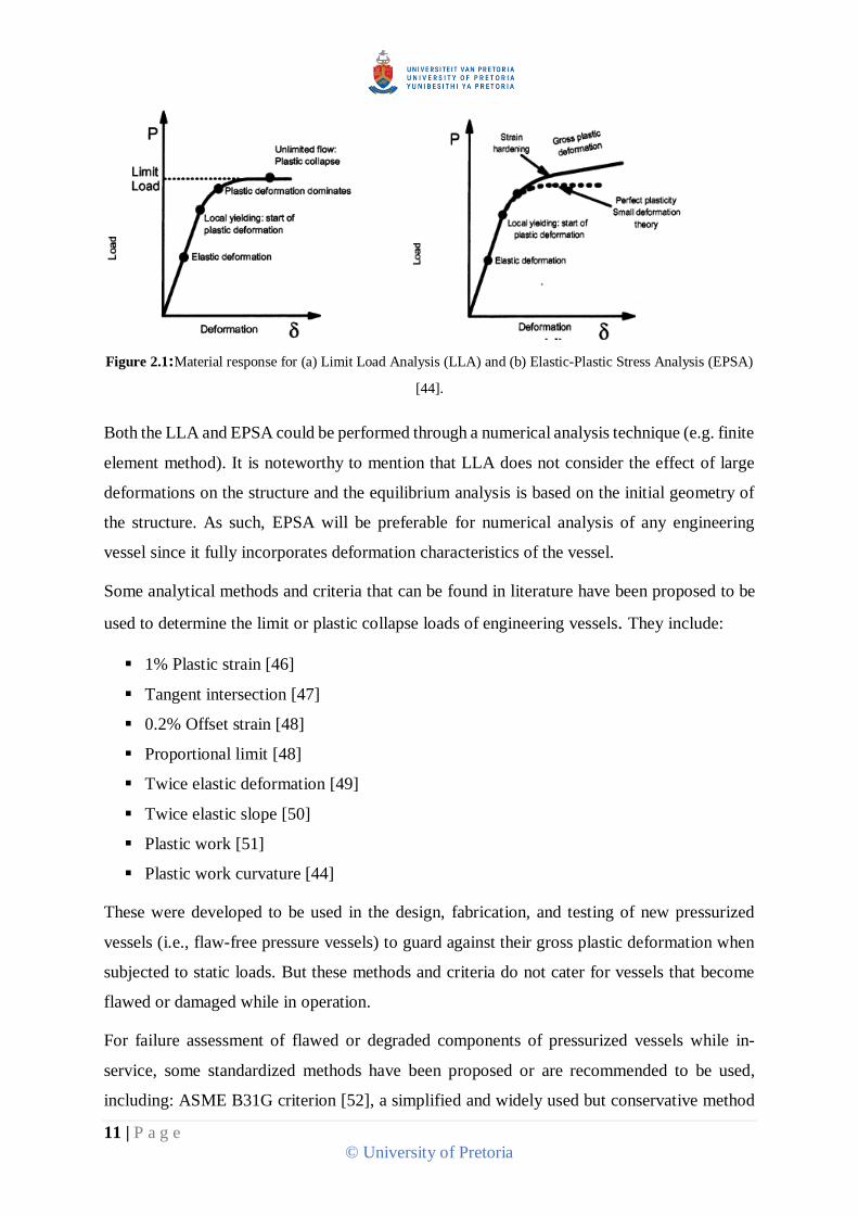
(ESA), Limit-Load Analysis (LLA) and Elastic-Plastic Stress Analysis (EPSA).

In ESA, stresses are obtained from an elastic analysis and classified into primary, secondary

and peak categories, which are then limited to specified allowable values such that plastic

collapse will not occur. Usually, this method gives a conservative prediction.

LLA assumes an ideal elastic-perfectly plastic material model and small (first order)

deformation theory. The material exhibits linear elasticity up to the yield stress, after which

small plastic strain develops followed by an unlimited plastic flow, occurring when it can no

longer maintain equilibrium with the externally applied load, as shown in Figure 2.1(a).

Accordingly, the limit load is therefore, the highest load that the structure can support before

there is a loss or violation of equilibrium between the external and internal forces [44,45]. The

allowable load that will prevent the plastic collapse of a vessel is then computed by applying a

design factor to the obtained lower bound limit load [34].

However, real engineering vessels (like boiler tubes) may behave differently to the LLA model

by exhibiting strain hardening and large deformations. In this situation, EPSA, incorporating

an elastic-plastic material model is used to obtain a plastic collapse load on which a design

factor is applied to obtain an allowable load that will prevent the onset of plastic collapse in

the vessel [34]. Based on this analysis, the material exhibits linear elasticity up to yield stress,

after which the stress and strain increase in a nonlinear manner supporting more loads beyond

the limit load without violating the vessel equilibrium, as shown in Figure 2.1(b). The plastic

load is determined as the load at which gross plastic deformation will occur within the vessel

[44].

11 | P a g e


Figure 2.1:Material response for (a) Limit Load Analysis (LLA) and (b) Elastic-Plastic Stress Analysis (EPSA)

[44].

Both the LLA and EPSA could be performed through a numerical analysis technique (e.g. finite

element method). It is noteworthy to mention that LLA does not consider the effect of large

deformations on the structure and the equilibrium analysis is based on the initial geometry of

the structure. As such, EPSA will be preferable for numerical analysis of any engineering

vessel since it fully incorporates deformation characteristics of the vessel.

Some analytical methods and criteria that can be found in literature have been proposed to be

used to determine the limit or plastic collapse loads of engineering vessels. They include:

1% Plastic strain [46]

Tangent intersection [47]

0.2% Offset strain [48]

Proportional limit [48]

Twice elastic deformation [49]

Twice elastic slope [50]

Plastic work [51]

Plastic work curvature [44]

These were developed to be used in the design, fabrication, and testing of new pressurized

vessels (i.e., flaw-free pressure vessels) to guard against their gross plastic deformation when

subjected to static loads. But these methods and criteria do not cater for vessels that become

flawed or damaged while in operation.

For failure assessment of flawed or degraded components of pressurized vessels while in-

service, some standardized methods have been proposed or are recommended to be used,

including: ASME B31G criterion [52], a simplified and widely used but conservative method

12 | P a g e


to predict the collapse (or burst) pressure and remaining strength of the vessels; Modified

ASME B31G criterion [53,54], an improved version of ASME B31G using a less conservative

flow stress, bulging factor and modified defect area; RSTRENG application program [53,55],

which computes the flaw area and uses the Modified ASME B31G to predict the failure

pressure of the vessels; PCORR [56–58], a finite element program that uses the 𝜎𝑢𝑡𝑠 and

ductile fracture criteria to assess the integrity of the vessels; DNV-RP-F101 [59], an assessment

guideline developed from a full-scale experimental test and FEA, and RPA [60], a method for

assessing the residual strength of the vessels. Other criteria and models developed by some

authors include: Chell limit load analysis [61], Kanninen axisymmetric shell theory model [62],

Ritchie and Last corrosion flaw criterion [63]. All these methods, models and criteria were

developed primarily to be used for fitness-for-service (FFS) assessment of corroded pipelines.

Failure Assessment of Locally Thinned Pressurized Vessels

For general cases of local metal loss, with reference mostly to internal metal loss, the following

assessment methodologies and criteria have been proposed by different authors:

2% Plastic Strain and the RSF Criteria

A parametric study was conducted by Sims et al. [64] using Elastic Plastic Finite Element

Analysis (EPFEA) on cylindrical and spherical shells with predominantly pressure loading and

containing round local thin areas (RTAs), which were remote from structural discontinuities

such as nozzles and head-to-shell junctions. An ideal elastic perfectly plastic model and a limit

of 2% plastic strain (𝑃2%) was used in this study to obtain a conservative estimate of the

collapse pressure. The data obtained from the study was used to compute a remaining strength

factor (RSF) to aid in the FFS evaluation of round thin areas in pressure vessels, piping and

storage tanks. The RSF was defined as:

RSF =Collapse Pressure of Flawed Component

Collapse Pressure of Unflawed Component (2.1)

An RSF of 0.9 or greater is considered to be acceptable. The study was extended to groove-

like local thin areas (GTAs) on spherical and cylindrical shells by Hantz et al. [65] using a

bilinear model with the yield stress set at 10% lower than the one used for the RTA case, and

the slope of the model set at a value equal to the yield strength at 𝑃2%. Results obtained from

the EPFEA were used to develop a screening/acceptance criterion for axial and circumferential

GTAs on cylinders and meridional GTAs on spheres.

13 | P a g e


Ultimate Tensile Strength (𝝈𝒖𝒕𝒔) and Ductile Fracture Criteria

Leis and Stephens [56] proposed assessing the integrity of corroded pipelines using the uniaxial

𝜎𝑢𝑡𝑠 as a reference failure stress. This produced more accurate prediction of failure pressures

compared to using the yield stress-based values in ASME B31G and RSTRENG methods, as

well as the uniaxial and multiaxial yield stress values. They used the work in [57] to develop

an alternative assessment criterion for metal-loss involving complex loadings, complex flaw

shapes, sizes and spacing via parametric analyses using a special purpose shell-based finite

element code known as PCORR and a ductile fracture criteria, which encapsulates the yield

stress ( 𝜎𝑦), 𝜎𝑢𝑡𝑠 and the fracture toughness of the pipe. Based on internal pressure loading,

the assessment method ranked the flaw depth and length as first order factors controlling the

failure behaviour of the eroded pipes, while the flaw width was ranked as a second order factor.

In another paper [58], the duo did a comparative investigation of the influence of material and

geometry factors on the failure pressure of blunt corrosion defects and local thin areas (LTAs)

in pipes. By employing existing experimental data, a ductile rupture criterion and parametric

FEA, they succeeded in ranking the relative contribution of each variable to the failure pressure

from most to least important as follows: Internal pressure, pipe diameter, wall thickness/flaw

depth, ultimate strength, flaw length, flaw shape characteristics, yield strength/strain hardening

characteristics, flaw width and fracture (Charpy) toughness.

Ultimate Tensile Stress ( 𝝈𝒖𝒕𝒔) and 95% 𝝈𝒖𝒕𝒔

Shim et al. [66,67] performed three dimensional FEA to simulate full-scale pipe tests conducted

for various wall-thinning geometries subjected to a combined loading (internal pressure and

bending moment). Failure was predicted by obtaining the maximum moment when the

equivalent stress in the thinned area reached the 𝜎𝑢𝑡𝑠. There was a good agreement when the

FEA results were compared with the experimentally generated maximum moment. Using the

same criterion, FEA were performed to investigate the effect of the internal pressure, wall-

thinned length, depth and angle on the maximum moment.

Fekete and Varga [68] investigated the load carrying capacity of transmission steel pipe lines

with external corrosion defects using a bilinear isotropic hardening material model in the

nonlinear FEA. The characteristic flaw was modelled as an ellipsoid shape on the surface of

the pipe. Burst pressure values were obtained from the analysis at the deepest point of the

corrosion defect, where the Von Mises equivalent stresses were equal to the 𝜎𝑢𝑡𝑠. These results

correlated well with the results obtained from experiment and semi-empirical methods. The

14 | P a g e


effect of the width to length ratio of flaws on the load carrying capacity of the pipes was also

examined.

Abdalla Filho and co-authors [69] used FEA to assess the accuracy of some analytical (semi-

empirical) models commonly used in the industry to predict the failure pressure of pipelines

containing wall reduction and isolated corrosion pit defects. An elastic-plastic model with

isotropic hardening and Von Mises yield criterion was used in their work. The pipe was

considered to have failed when the stress developed within the flawed area was equal to the

pipe 𝜎𝑢𝑡𝑠 or when local plastic collapse occurred. The corresponding pressure was taken as the

failure pressure. The semi-empirical models and finite element shell models were validated by

comparing their results to that of experimental data from the literature. The results show that

semi-empirical methods are generally conservative when applied on short corrosion defects.

The authors concluded that ASME B31G and RPA methods may be recommended for both

short and long flaws assessment, RSTRENG 0.85 dL methods for short defects assessment

only and the DNV RP-F101 model for long flaws assessment only.

Yeom et al. [70] established a corrosion defect assessment method for API X70 pipe via a full-

scale burst test and FEA. The burst pressure results of the FEA were compared with results

from popular analytical models used in the industry for different depth to thickness ratios at

25%, 50% and 75%. The failure behavior and burst pressures obtained from the full-scale test

and FEA (at the point which the internal pressure reaches 95% of the 𝜎𝑢𝑡𝑠) were analyzed and

compared, leading to the development of an integrity evaluation regression equation for the

defected area.

True Ultimate Tensile Strength (𝝈𝒕,𝒖𝒕𝒔) and 90 % 𝝈𝒕,𝒖𝒕𝒔

J. W. Kim et al. [71] did a series of tensile tests on notched bar specimens with varied notch

radii. This was followed by finite element simulations to evaluate the stress and strain within

the notched area of the specimens under internal pressure, which corresponds to their maximum

load and final failure. From the results, the authors developed two local failure criteria (stress-

and strain-based) that could be used to predict the maximum load carrying capacity and final

failure for local wall-thinning in piping components. The stress-based criterion is based on the

true ultimate tensile stress(𝜎𝑡,𝑢𝑡𝑠), while the strain-based criterion is a function of stress

triaxiality. Both criteria gave similar agreement with the experiment result, but the stress-based

criterion was more accurate than the strain-based criterion, which overestimated the failure

pressure of the pipes.

15 | P a g e


Ma et al. [72] carried out an assessment on the failure pressure of high strength pipelines (HSP)

with external corrosion defects. First, they developed a theory to deduce the failure pressure of

end-capped and unflawed pipes using the Von Mises failure criterion and Ramberg-Osgood

hardening stress-strain relationship. They proceeded to do an extensive FEA for different

geometrical sizes of the elliptical corrosion defect modelled on the pipe leading to a general

solution for assessment of corroded HSP. This was done by considering the variation trend (via

regression analysis) of the obtained burst pressure values when the Von Mises equivalent stress

reaches 𝜎𝑡,𝑢𝑡𝑠 of the steel. The outcome of their work was a new formula for predicting the

failure pressure of corroded HSP. Results from the FEM were validated using 79 burst test

samples involving low, mid, and high strength grade steel pipelines. The comparison showed

that the predicted failure pressure is much closer to the actual burst pressure in HSP and for the

mid-grade strength pipelines, but not reliable for low-grade strength pipelines.

Y.P Kim et al. [73] evaluated an X65 pipe that contained specially machined rectangular

corrosion defects via full scale burst tests and FEA. For the simulation, failure was assumed to

occur when the Von Mises stress at the defect area reached the reference stress value of 90%

of the 𝜎𝑡,𝑢𝑡𝑠 . The limit solution for corrosion defects within the girth weld and seam weld of

pipe was proposed as a function of corrosion length and depth based on the PCORR criterion

by applying regression analysis on the FEA results.

Flow Stress

Kamaya et al. [74] investigated the failure pressure of a straight pipe with wall thinning

subjected to internal pressure via 3D elastic-plastic FEA for small and large deformations.

Three kinds of materials were considered in the analyses (line pipe steel, carbon steel, and

stainless steel) and wall thinning was assumed to be of circumferentially uniform depth inside

the pipe. The line pipe steel was observed to have the lowest failure pressure after normalizing

its failure pressure by that of the unflawed pipe using flow stress (which is the average of the

𝜎𝑦 and 𝜎𝑢𝑡𝑠) as reference. The authors were able to show that with the assessment curves

generated for line pipe steel, conservative estimates could be made for carbon steel and

stainless steel. In another paper [75], they examined the influence of normalizing the flaw

length on the failure pressure of pipes with localized thinning by conducting burst tests and 3D

elastic-plastic FEA. The FEA was parameterized for various dimensions of pipes, flaw lengths

and depths to study their effects on the failure pressure of the pipe. It was observed that the

burst pressure decreases as the flaw length increases and in normalizing the effect of flaw

16 | P a g e


length on failure pressure, it was more appropriate to normalize the flaw length by the pipe

mean radius (𝑅) of the unflawed area rather than its shell parameter (√𝑅𝑡) with a pipe thickness

(𝑡), as is usually done.

Yield, Flow, and Ultimate Tensile Strengths

Choi, et al. [76] proposed limit load solutions for X65 steel-type corroded pipelines by

conducting a series of burst tests and finite element simulations. Two types of defect geometries

were considered (rectangular and elliptical shapes). Reference stresses were set to:

Yield Strength, 𝜎𝑦

Ultimate Tensile Strength, 𝜎𝑢𝑡𝑠

Flow Strength, 𝜎𝑓 , [𝜎𝑓 = (𝜎𝑦 + 𝜎𝑢𝑡𝑠) 2⁄ ]

80% and 90% of 𝜎𝑢𝑡𝑠

These were all used as failure criteria. Failure was assumed to occur when the Von Mises stress

distribution across the defected area reached the reference stress to which the corresponding

internal pressure was taken as the failure pressure. Resulting failure pressures were normalized

with corresponding experimental burst pressures. The best prediction for the elliptical shaped

defect was at the reference stress of 80% of 𝜎𝑢𝑡𝑠, and for the rectangular defect, 90% of 𝜎𝑢𝑡𝑠.

In comparison to the FEA solutions, the modified B31G results gave conservative estimates

for shallow and short corrosion flaws but was non-conservative for deep and long flaws.

Boiler Tubes Localized Erosion Failures

It is noteworthy that though failure assessment criteria and methodologies for localized

thinning or metal-loss in pressurized vessels have drawn a lot of attention over the years due

to the associated failure implications of engineering structures, many of these studies have been

focused on internal wall loss mechanisms associated with these vessels [55,62,65,69,76–80].

Only a few studies associated with developing failure criteria or methodology for localized

external erosions in boiler tubes have been done. A key contribution in this area has been the

scholarship of Zarrabi and colleagues [10,11,16,21].

Zarrabi [10,16,81] first developed a simple method to estimate the life of boiler tubes in fossil-

fuel power plants. The method applies in cases where the failure mode is dominated by creep

rupture and/or plastic collapse with fracture in the presence of tube thickness loss driven by

corrosion and/or erosion processes. He formulated a computation for the plastic collapse,

reference stress of the tube, its thinning rate and creep rupture time. He noted that in the absence

17 | P a g e


of creep, the reference stress will be equal to the flow stress, which is the average of 𝜎𝑦

and 𝜎𝑢𝑡𝑠. An algorithm for computing the remaining life of the tube was also documented. The

author also carried out a comparison with three other boiler tube life prediction methods, of

which the method he proposed was better at predicting the tube life.

Zarrabi and Zhang [21] performed an elastic-plastic finite element analyses (EPFEA) to obtain

primary stresses in the localized thinned area of a tube. From their study, they came up with a

parameter (P∗) that when multiplied with the primary stress in the unflawed area results in the

primary stress of the flawed area. P∗ was defined as:

P∗ = Plastic Collapse Pressure of a Tube with Uniform Thickness

Plastic Collapse Pressure of the Tube in the Local Thin Area (2.2)

It was computed from the EPFEA of a tube with a part-through rectangular slot (flaw) using

an elastic-perfectly plastic material model and a Von Mises yield criterion. P∗ values were also

computed for an elliptical flaw, triangular flaw and a double rectangular flaw. Results from

these analyses were compared using their plastic collapse pressures and radial displacements

at the deepest point of the flaw area. The triangular flaw had the highest collapse pressure

value.

Zarrabi and Zhang [11] also described a method for life and failure thickness assessment of

boiler tubes with localized pits and coded the method into a computer program referred to as

‘AUSI-TLI’. With this program, the tube remaining life, critical tube thickness and critical

stress were assessed and evaluated.

In the work of Zarrabi and Zhang, the estimated creep and plastic collapse life they computed

used a conservative reference failure stress derived from multiplying a semi-empirical non-

dimensional parameter to account for the variation of the scar geometry with the Von Mises

stresses of an undamaged tube, along with the tube material properties and operating conditions

[10,11,81]. This model cannot be relied upon because of its over-conservativeness.

Gong et al. [30] investigated some ruptured titanium tubes that were obtained from a power

plant by microscopic analyses and FEA. This was performed to evaluate the effect that stresses

from degradation processes (such as clogging, erosion and fretting) exerted on the wall of the

tubes. Also, from the result of the FEA, they were able to deduce the extent of degradation of

the tubes and suggest some preventive measures.

18 | P a g e


DePadova et al. [82] performed FEA on the local thin areas (narrow and wide grooves) on two

pressure vessels. The FEA results that included strain hardening reasonably predicted the

plastic strains associated with the failure of these vessels, which were in good agreement with

the test data, while the elastic perfectly plastic FEA results were conservative.

FEA was also used by Kim et al. [83], for the burst failure prediction of a plain seamed tube, a

second tube with a weldment, and a third one with a heat affected zone, all made to bulge under

combined internal pressure and axial loading. The outcome of their analyses showed some

feasibility of predicting an initial fracture initiation and bursting pressures of these tubes.

In a study by Othman et al. [84], superheater tubes were modelled, and the maximum stress

induced by the deformed tube was obtained. The results obtained had a good correlation with

those obtained from the power plant.

Visual examination and microscopic analyses that includes SEM, EDS and XRD were carried

out by Dini et al. [85] on some tubes with oxide scales. Numerical analysis of these tubes under

continuous annealing were also carried out to determine the effect of increased temperature on

the tube life as well as the extent of damage in the tubes. The result of the analysis indicated

the potential of the damaged region in the tubes to be prone to high temperature creep failure.

Purbolaksono et al. [86], carried out failure case studies on SA 213-T22 reheater and

superheater steel tubes. They used finite element simulations with iterative methods to estimate

the remaining life of the tubes. This was done by tracking the increased temperature and

decreased hardness due to cumulative creep damage, i.e., as oxide scales grow on their inner

surface of the tubes over a long period. The estimations obtained show some good agreement

with the experimental data retrieved from the reports on the failed tubes and could provide

forewarning to enable prior action to be taken before failure occurs. In a similar study,

Purbolaksono et al [87] used the average growth rate of the oxide scales in some reheater tubes

to model 2D axisymmetric geometries using MSC PATRAN/NASTRAN and some

measurements obtained from the tube samples. The results from the FEA were reported to be

in good agreement with the microscopic inspections carried out on the tubes.

Though the above works have showed some progress in using FEA for failure assessment of

boiler tubes, a focused study on which flaws in boiler tubes are most at risk of failure due to

plastic collapse has not been done. Detailed studies are needed to able to rank detected flaws

from most severe to least severe. This would allow operators to optimize the available

19 | P a g e


maintenance budget and focus attention where necessary, reducing the likelihood of

unexpected outages.

API-ASME Fitness-For-Service (FFS) Assessments

As noted earlier for common analytical methods and criteria, design codes and standards for

pressurized vessels that have been in existence often provide rules and analyses for the design,

manufacturing, inspection, and testing of new pressurized equipment (pressure vessels, pipes

and storage tanks) but do not provide rules for evaluating these equipment while they degrade

in service or become deficient due to the presence of a flaw or damage. But in recent years, the

American Petroleum Institute (API) and the American Society of Mechanical Engineers

(ASME) have made efforts to develop a standard document built from previous local thin area

(LTA) failure assessment criteria and methodologies that will provide some guidance towards

carrying out quantitative engineering assessments to demonstrate the structural integrity of

components of pressurized vessels, containing damage or a flaw while in use.

API 579 assessment guide

Anderson and Osage [88] presented an overview of the API Recommended Practice 579 [89],

which was the first document for FFS assessment guide for pressurized vessels. API 579 was

designed to provide guidance for conducting FFS assessments of a wide range of flaws and

damage mechanisms (such as brittle fracture, cracks, metal-loss, pitting corrosion, blisters,

weld misalignment, etc.) that usually occur in pressure vessels, piping, and storage tanks

encountered in petrochemical and other processing industries. The guidelines provided in API

579 were to enable plant inspectors and engineering personnel to make decisions to rerate,

repair, replace or retire the flawed component under assessment. The authors described the

organization of the API document, the three levels used in the assessment methodology and

the rerating and remaining life calculations. Similarly, Janelle and Osage in 2007 reviewed the

technical basis for the fitness-for-service assessment procedures for general and local metal

loss in API 579. Validation of the procedures and additional methods developed for analyzing

and evaluating LTAs were discussed and recommended to be included in the API 579 standard.

API 579-1/ASME FFS-1 and API 579-2/ASME FFS-2 assessment guides

The methodology and criteria documented in the API 579 Standard document were tailored for

structural components used in the refining and petrochemical industries. A few years after,

ASME and API jointly came up with one standard document in two parts (referred to as API

579-1/ASME FFS-1 and API 579-2/ASME FFS-2 assessment guides) [90,91] to provide

20 | P a g e


guidelines for FFS assessment for a wide range of in-service structural components used in

process, manufacturing, and power generation industries. The first part explains the

methodologies to be used for the FFS assessment while the second part documents some

practical example problems. A newer edition, which include some modifications and additional

assessments was released in 2016 [33].

The standard provides for three levels of assessment for evaluating LTAs, which are Level 1,

2 and 3, just like in the API 579. Generally, each level presents a balance between the

information required for the evaluation, conservatism, personnel skill performing the

evaluation and the complexity of the assessment being performed. Level 1 is the most

conservative. The procedures contained in this level are envisaged to provide conservative

assessment criteria that can be performed using a minimum amount of component information

and inspection. There is also a limiting flaw size that can be evaluated using this level, which

makes it unsuitable for components with complex geometry and/or complex loading. As it is

not a detailed analysis, a plant inspector or an engineering personnel could perform this level

assessment.

Level 2 assessment procedures are intended to present a more detailed evaluation that produces

less conservative outcomes compared to those from Level 1 evaluation. Similar amount of

component information and inspection with that of Level 1 assessment are required for this

level assessment, as well as more detailed calculations. Flaw geometries that could not be

assessed using Level 1 can be evaluated, though would still be limited for complex flaw

geometries. The Level 2 assessment is usually performed by plant engineers or engineering

specialists that are knowledgeable and experienced in conducting FFS evaluation.

The Level 3 assessment procedures are intended to provide the most accurate evaluation of all

the three levels. As the levels increase from 1 through to 3, the amount of conservatism

associated with their methodologies decreases, making the Level 3 assessment the most

precise. Level 3 assessment requires the most detailed component information and inspection,

with the proposed analysis to be based on a numerical technique (such as FEM) or experimental

technique if necessary. As such, engineering specialists that are skilled and experienced in

conducting FFS evaluation are usually those who would perform this level of assessment. From

the API-ASME FFS, protection against plastic collapse is typically a stress analysis method,

which could either be a linear or nonlinear stress analysis, similar to the procedures documented

in the recent ASME Design Standard [34] as reported earlier in Section 2.2.1, only with

additional difference since the analysis is to be carried out on flawed components.

21 | P a g e


In this case, the LLA employs numerical analysis using small displacement theory and an

elastic-perfectly plastic material model set at a specific yield strength of 1.5𝜎𝑎. The 𝜎𝑎 is the

allowable stress, which is typically a fraction of yield, tensile or rupture stress at room and

service temperatures. For the EPSA, an elastic plastic material model, large displacement

theory (to account for the effect of nonlinearity) and a true stress-strain hardening material

model, which is temperature dependent, are used. This ensures that in the model, the hardening

behavior gets up to the true ultimate tensile stress (𝜎𝑡,𝑢𝑡𝑠). Beyond this, the behaviour is

perfectly plastic. The EPSA provides a more accurate FFS assessment, as it considers the

redistribution of stress that occurs due to the plastic deformation of the flawed components,

and their deformation characteristics.

For the FFS assessment using nonlinear analysis, the concept of Load and Resistance Factor

Design (LRFD) is suggested as an alternative to be used instead of determining the plastic

collapse load of the vessel [33]. For the LRFD, different factored load combinations, based on

the loads the vessel is subjected to, are used for the numerical analysis. For the case of internal

or external pressure only, the required factored load combinations are given as follows:

Factored Load for Limit Load Analysis = 1.5. 𝑃𝑚𝑎𝑥 . 𝑅𝑆𝐹𝑎 (2.3)

Factored Load for Elastic Plastic Analysis = 𝛽. 𝑃𝑚𝑎𝑥 (2.4)

where 𝑃𝑚𝑎𝑥 is the Internal or External Maximum Allowable Working Pressure, 𝑅𝑆𝐹𝑎 is the

Allowable Remaining Strength Factor with a recommended value of 0.9 (the value can be more

or less conservative depending on the design codes used for the vessel construction, type of

loading and/or consequence of failure), and 𝛽 is the Load Factor Coefficient based on the factor

applied to the 𝜎𝑢𝑡𝑠 to obtain a design allowable stress, (the value varies for different

construction codes). For pressure vessels designed using ASME Section VIII, Division 2 prior

to the 2007 edition, 𝛽 = 3. 𝑅𝑆𝐹𝑎. Based on these guidelines, the factored load combinations to

be used for the limit load analysis becomes 1.35. 𝑃𝑚𝑎𝑥 and that of the Elastic Plastic Analysis

is 2.7. 𝑃𝑚𝑎𝑥.

The analyses are to be performed using these factored loads and if convergence is attained, that

indicates the component being analysed is stable under the applied load. If not, its thickness

shall be modified or the applied loads reduced, and the analysis is repeated until convergence

is attained.

22 | P a g e


Another approach described in the document for evaluating LTAs is using the Remaining

Strength Factor, RSF, which was first proposed by Sims [64]. This was expressed as:

𝑅𝑆𝐹 = Limit or Plastic Collapse Load of the Flawed Component

Limit or Plastic Collapse Load of the Unflawed Component (2.5)

Based on the outcome of the RSF, the component analysed can be recommended to continue

to be used as it is or to be repaired or the Maximum Allowable Working Pressure of the Flawed

Component (MAWP) evaluated and altered or rerated using the Maximum Allowable Working

Pressure of the Unflawed Component (𝑀𝐴𝑊𝑃𝑜). These quantities are as expressed [33]:

𝑀𝐴𝑊𝑃 = 𝑀𝐴𝑊𝑃𝑜 (RSF

RSFa) for 𝑅𝑆𝐹 < 𝑅𝑆𝐹𝑎 (2.6)

𝑀𝐴𝑊𝑃 = 𝑀𝐴𝑊𝑃𝑜 (RSF

RSFa) for 𝑅𝑆𝐹 ≥ 𝑅𝑆𝐹𝑎 (2.7)

A decision can also be made to retire the analysed tube if the RSF outcome is too low.

Challenges with the API 579 and ASME FFS Assessment Guides

Though the elastic-plastic analysis method as proposed in the FFS document is the most

reliable guide for localized thinning evaluation, it still presents some challenges. First, detailed

inspection and component information is required before doing the analysis, not only for level

3 assessment but for the other two levels as well. Second, cumbersome FEA simulation is

required each and every time you need to do an assessment for a particular flaw, which must

be performed by an experienced engineering specialist. In fact, before the level 3 assessment

will be performed, the detected localized flaw on the vessel would have undergone the rigors

of level 1 and 2 assessments and certified to have failed to meet their acceptability criteria.

These challenges are time consuming and financially expensive to cater for.

Also, with the concept of LRFD as suggested to be used for the FEA, there is still the rigor of

setting up and running a detailed FEA for each localized flaw to be assessed in this level. To

avoid computing plastic collapse loads, which could consume computational resources and

time, the factored loads that were proposed as reasonable estimates are empirical and as such,

has the capability to still give relatively conservative plastic collapse results.

Based on the above issues, there is, therefore, a need to develop a new, less complex and less

expensive methodology that could be used to rapidly categorize the severity of localized

external erosion flaws in boiler tubes and guide maintenance decisions on these critical assets.

23 | P a g e


Summary and Conclusions

In this chapter, the initial studies that led to the development of various criteria and

methodologies for assessing failures in pressure vessels were discussed. Previous studies from

a general perspective of failure analysis of pressurized vessels to studies on failure assessments

of flawed pressure vessels, as well as assessment of localized thinned vessels were all discussed

in details. The chapter also reviewed methodologies and criteria proposed by various authors

that could be used for evaluating pressurized vessels and guard against their plastic collapse

while in use. These criteria include:

2% Plastic strain

RSF Criteria

𝜎𝑢𝑡𝑠

95% 𝜎𝑢𝑡𝑠



Ductile Fracture Criteria

𝜎𝑡,𝑢𝑡𝑠

90 % 𝜎𝑡,𝑢𝑡𝑠

𝜎𝑦

Flow Stress, 𝜎𝑓.

Numerical studies that have been carried out on localized thinning in boiler tubes were

discussed. Though these finite element studies were performed to determine the root cause of

these failures and provide some preventive measures to avoid their reoccurrence, yet more

detailed study is needed to provide a rapid decision-making tool to guide in categorizing the

severity of these defects. The API-ASME fitness-for-service assessment guides recently

proposed to be used were also discussed and the challenges inherent in them were highlighted.

From the review, it is apparent that more detailed studies are needed to avoid replacing tubes

that could still be safe for continued operation, while also guarding against the failure of the

tubes, their emergency costly repairs and forced outages. The next chapter presents the

modeling procedures for some conceptualized flawed tubes, the geometric definition of the

modelled flaws and the technique that can be used to replicate real flawed tubes on these

conceptualized models.

24 | P a g e


3 MODELLING OF LOCALIZED THINNED TUBES AND

GEOMETRIC DEFINITIONS OF THE FLAWS

Introduction

The first procedure to carrying out a detailed investigation on localized external eroded tubes

is to create geometric models in a way that is sufficiently flexible and could reasonably capture

real flaw geometries that exist in practical scenarios. In this chapter, the modeling of some

conceptualized variants of tubes having geometrical shapes of localized external erosion that

could possibly occur in real scenarios is presented. The formulation of geometry functions from

these conceptualized models to enable the accurate modelling of real localized thinned tubes

and aid in their detailed failure assessment is documented. The process of replicating real tubes

on these developed geometries is also discussed.

Modelling of Conceptualized Flawed Tubes

Previous FEA studies on boiler tubes were done using flaw geometries such as: elliptical scar,

triangular scar, rectangular scar, double rectangular scar and part-through rectangular scar

[11,21,81] as can be seen in Figure 3.1. These flaw geometries do not resemble practical

scenarios of localized external erosion. Other defects modelled on erosion of titanium tubes in

heat exchangers [30] and as corrosion defects on pipes [68] were more suitable as seen in Figure

3.2.

Figure 3.1: (a) Various modelled flaw shapes on boiler tubes [21] and (b) Part-through rectangular modelled

flawed tube [21,81].

25 | P a g e


Figure 3.2: Modelled elliptical erosion defect of a titanium tube [30] and (b) corrosion defect on a pipe [68].

To mimic real types of localized thinned flaws that could possibly occur in practical scenarios,

three conceptualized variants of localized thinned areas having a specific flaw depth, 𝑓𝑑 are

created on an open-ended flawed tube modelled in ANSYS® using the DesignModeler. Figure

3.3 shows a modelled tube having a localized thinned area (LTA), with flaw length (𝑓𝑙) and

flaw width (𝑓𝑤) as the LTA dimensions.

Figure 3.3: Sample of a modelled tube showing the localized thinned area.

The three variants are created by sweeping a flat line, a concave and a convex elliptical surfaces

as described below in details.

The first variant referred to as the flat line flaw is made by first offsetting a plane, height, 𝐻

from the centre line of the tube and sketching a horizontal straight line at the specific flaw

depth, 𝑓𝑑 . The sketch is revolved about the x-axis from the position of the plane to slice and

cut the tube to the 𝑓𝑑 as shown in Figure 3.4 to Figure 3.6.

𝑓𝑙

𝑓𝑤

l

26 | P a g e


Figure 3.4: Schematic showing the modelling of a flat line flawed tube - cross-section

Figure 3.5: Pictorial representation in ANSYS® showing the plane axis offset from the centre line of the tube, the

sketched horizontal line and the flat line modelled flaw

𝑓𝑑

Centre line of tube

x

y

𝐻

27 | P a g e


Figure 3.6: A flat line flawed tube

The second modelled localized flaw on the tube is a u-shaped or scoop shaped flaw, created

by offsetting a plane from the centre line of the tube to a height, 𝐻, then sketching from the

mid-axis of the tube a convex ellipse with an axis offset by a height, 𝑧 from the tube centre

line. This makes the ellipse intersect the circular cross section of the tube in a u-shaped manner.

The sketch is revolved from the plane axis at 𝐻 in the horizontal direction to slice-cut the tube

to a specific 𝑓𝑑 as shown in Figure 3.7 to Figure 3.9.

The third variant referred to as the n-shaped or saddle shaped flaw is made by first offsetting

from the tube centre line to a height, 𝐻, then sketching a concave ellipse that is offset from the

base to a height, 𝑧 and also two vertical straight lines drawn from the plane to the vertices of

the ellipse. This causes the ellipse to intersect the circular cross section of the tube in an n-

shaped manner. The entire sketch is revolved about the x-axis from the vertical plane and

sliced-cut to the required flaw depth, 𝑓𝑑 on the tube as shown in Figure 3.10 to Figure 3.12.

28 | P a g e


Figure 3.7: Schematic showing the modelling of a u-shaped flawed tube - cross-section.

Figure 3.8: Pictorial representation in ANSYS® showing the plane axis offset from the centre line of the tube, the

sketched convex ellipse and the u-shaped flaw.

𝑧

Centre line of tube

x

y

𝐻

𝑓𝑑

29 | P a g e


Figure 3.9: A u-shaped flawed tube.

Figure 3.10: Schematic showing the modelling of an n-shaped flawed tube - cross-section.

𝐻

Centre line of tube

𝑓𝑑

z

x

y

30 | P a g e


Figure 3.11: Pictorial representation in ANSYS® showing the plane axis offset from the centre line of the tube,

the sketched concave ellipse and the n-shaped flaw.

Figure 3.12: An n-shaped flawed tube.

After the creation of the flaw geometry on the model, it is sliced three times through each of

the base planes (XY, ZX, and YZ Planes) in ANSYS. The outer flaw surface of the tube is then

deleted, and the flaw surface extruded through a slice operation in the reversed direction to a

31 | P a g e


depth greater than or relatively less than the tube thickness, depending on the shape of the flaw.

Based on symmetry conditions of the FEM, three quarter of the model is deleted, leaving a

quarter model to be used for the analysis as shown in Figure 3.13 (a). This is done to save

computation time during the analysis. The flaw area is further sliced from the YZ base plane

through the Z axis that is offset to half of the 𝑓𝑤 , to facilitate the easy application of mesh

control measures within the flaw area during the mechanical analysis. Figure 3.13 (b) shows

the sliced flawed tube.

Figure 3.13: Quarter n-shaped finite element model showing (a) the extruded flaw area and (b) the sliced flaw

area.

Geometric Definition of the Flaws

Having developed these conceptualized flawed tubes, it is necessary to generate some geometry

functions from these conceptualized models that will enable the accurate modelling of real

localized thinned tubes to carry out NLFEA and parametric studies for their failure assessment.

The mathematical expressions for the tube flaw geometries: the flaw length (𝑓𝑙), flaw

width (𝑓𝑤), and flaw depth (𝑓𝑑) are formulated for a tube with an outer diameter (𝐷𝑜) and tube

thickness (𝑡) using the following parameters:

Plane height from the centre line of the tube (𝐻)

Radius of the cutting plane from the plane axis (𝑅)

Horizontal dimension of the elliptical surface (𝑎)

Vertical dimension of elliptical surface (𝑏)

Remaining thickness of the tube (𝑡𝑟)

32 | P a g e


Computing the flaw length, 𝒇𝒍

The 𝑓𝑙 of the flawed tube, which is the same for all three variants is derived from the schematic

shown in Figure 3.14

Figure 3.14: Schematic showing the creation of the localized flaw length on the tube – side view.

The cutting radius, 𝑅 is given by:

𝑅 = 𝐻 – [(𝐷𝑜

2) − 𝑓𝑑] (3.1)

By Pythagorean Theorem,

𝑅2 = (𝑅− 𝑓𝑑)2 + (

𝑓𝑙

2)2 (3.2)

Rearranging to solve for 𝑓𝑙 ,

𝑓𝑙 = 2√𝑅2 − (𝑅− 𝑓𝑑)2 (3.3)

which simplifies to:

𝑓𝑙 = 2√2𝑅𝑓𝑑 − 𝑓𝑑2

(3.4)

Computing the flaw width, 𝒇𝒘 for the flat-line flaw

The 𝑓𝑤 of the flat line flaw is derived from the schematic showing the intersection of the flat

line with the circular cross section of the tube shown in Figure 3.15.

𝑡𝑟

Centre line of tube

𝐻

𝑅

𝑓𝑙

𝑅

𝑓𝑑 𝑡

33 | P a g e


Figure 3.15: Front view of the flat line flaw showing the cutting plane in red, intersected with the tube cross-

section.

Applying Pythagoras,

(𝐷𝑜

2)2 = ((

𝐷𝑜

2)− 𝑓𝑑)

2 + (𝑓𝑤

2)2 (3.5)

Rearranging to solve for 𝑓𝑤 ,

𝑓𝑤 = 2√(𝐷𝑜

2)2 − ((

𝐷𝑜

2)− 𝑓𝑑)2 (3.6)

which simplifies to:

𝑓𝑤 = 2√𝐷𝑜𝑓𝑑 − 𝑓𝑑2

(3.7)

Computing the flaw width, 𝒇𝒘 for both the u-shaped and n-shaped flaws

The 𝑓𝑤 of the u-shaped flaw is derived from the schematic showing the intersection of the

convex ellipse with the circular cross section of the tube as shown in Figure 3.17. While the 𝑓𝑤

of the n-shaped flaw is derived from the schematic showing the intersection of the concave

ellipse with the circular cross section of the tube as seen in Figure 3.16. Tubes with 𝑓𝑤 𝐷𝑜⁄

dimension ratio of less than 0.5 are u-shaped flaws while others above 0.5 are n-shaped flaws.

𝐻

𝑅

Centre line of tube

Plane Axis

𝐷𝑜2

𝑓𝑤

𝑓𝑑

34 | P a g e


Figure 3.16: Front view of the u-shaped flaw showing the cutting plane in red, intersected with the tube cross-

section.

From Figure 3.16,

𝑓𝑑 = 𝐷𝑜

2− (𝐻 − 𝑅) (3.8)

𝑓𝑑 = 𝐷𝑜

2− (𝑧 − 𝑏) (3.9)

𝑅 = 𝐻 − (𝑧 − 𝑏) (3.10)

Figure 3.17: Front view of the n-shaped flaw showing the cutting plane in red, intersected with the tube cross-

section.

𝑧

𝑏

𝑎

𝑓𝑤

𝐻

𝑅

𝑓𝑑

𝐷𝑜2

Plane Axis

Centre line of tube

𝑓𝑑

𝑧

𝑏

𝑎

𝐻

𝑅

𝑓𝑤

Plane Axis

Centre line of tube

𝐷𝑜

2

35 | P a g e


From Figure 3.17,

𝑓𝑑 = 𝐷𝑜

2− (𝐻 − 𝑅) (3.11)

𝑓𝑑 = 𝐷𝑜

2− (𝑧 + 𝑏) (3.12)

𝑅 = 𝐻 − (𝑧 + 𝑏) (3.13)

To formulate the mathematical expression for the 𝑓𝑤 , the point of intersection on the x-axis of

the circle and ellipse need to be determined. The two simultaneous equations below are

considered:

For the circle:

𝑥2 + 𝑦2 = 𝑟𝑜2 (3.14)

For the ellipse:

𝑥2

𝑎2+

(𝑦−𝑧)2

𝑏2= 1 (3.15)

By solving these two equations (as documented fully in Appendix A), the value of the 𝑓𝑤 in

terms of 𝑥 is obtained from:

𝑥 = √−𝐵±√(𝐵2−4𝐴𝐶)

2𝐴 (3.16)

𝑤ℎ𝑒𝑟𝑒 𝐴 = (1 −𝑏2

𝑎2)2

; 𝐵 =4𝑏2𝑧2

𝑎2+ 2(1 −

𝑏2

𝑎2) (𝑏2 + 𝑧2 − 𝑟𝑜

2); 𝐶 = (𝑏2 + 𝑧2 − 𝑟𝑜2)2 − 𝑏2𝑧2

From Eq. (3.16), 𝑓𝑤 of either the n-shaped flawed tube or the u-shaped flawed tube can be

computed as 𝟐𝒙 for their full dimension, as shown below:

2.

√

−4𝑏2𝑧2

𝑎2+ 2(1 −

𝑏2

𝑎2) (𝑏2 + 𝑧2 − 𝑟𝑜

2) ±√((4𝑏2𝑧2

𝑎2+ 2(1 −

𝑏2

𝑎2) (𝑏2 + 𝑧2 − 𝑟𝑜

2))

2

− 4(1−𝑏2

𝑎2)2

𝐶 = (𝑏2 + 𝑧2 − 𝑟𝑜2)2− 4𝑏2𝑧2)

2 (1−𝑏2

𝑎2)2

These developed mathematical expressions allow for the determination of the 𝑓𝑙, 𝑓𝑤 and 𝑓𝑑 , as

functions of the model parameters, which is instrumental for the failure assessment of the tubes.

36 | P a g e


Technique used to Extract Flaw Geometric Properties of Real Failed

Tubes.

The equations defined in Section 3.3 allow the flaw geometric properties (𝑓𝑤 , 𝑓𝑙, 𝑡𝑟) to be

determined from the parameters of the cutting ellipse (𝐻, 𝑅, 𝑎 and 𝑏). However, to model a

specific real flaw for which the flaw geometric properties are known, the cutting ellipse

parameters need to be determined. This is a simple inverse problem. A built-in optimization

nonlinear function in MATLAB® [92] known as fminsearch that can find the minimum of

a function of several variables in an unconstrained domain is used to obtain the flaw geometric

properties of real localized thinned tubes in order to precisely model them. The function

expression used is shown below:

[xopt,fopt]=fminsearch('FitPipeFnx',[H R a b]) (3.17)

where xopt is the returned optimized output, fopt holds the returned value of the objective

function, FitPipeFnx represents the function to be minimized, which in this case is the

error between the measured flawed tube geometric dimensions and the computed flawed

tube geometric dimensions from the derived mathematical expressions. H, R, a, b, are the

starting input variables used.

The codes for the implementation of this technique and the FitPipeFnx function can be

found in Appendix B. The program also contained codes that constructed the shape of the

flawed tubes as they solved, which helped in deducing whether the obtained solution is

realistic. A good initial estimate for the starting variables is needed in order to effectively use

it. Table 3.1 shows the flaw geometric properties obtained using this technique for three real

cases of failed tubes [93].

Table 3.1: Flaw geometric properties extracted from three real failed tubes using the optimization technique.

Tube

No

Tube and flaw properties Input parameters

𝐷𝑜 (mm)

𝑡 (mm)

𝑡𝑟

(mm)

𝑓𝑙 (mm)

𝑓𝑤

(mm) 𝐻

(mm) 𝑅

(mm) 𝑎

(mm) 𝑏

(mm)

1. 75.0 7.0 0.50 600 20 6957.333 6926.333 30.013 89.990 2. 50.8 4.4 0.30 80 25 218.477 197.177 105.101 114.305

3. 50.8 4.4 0.17 70 40 168.088 146.911 25.191 14.062

37 | P a g e



In this chapter, geometric variants of localized thinned tubes with real geometries, as could be

seen in actual scenarios were modelled. Geometric functions that could help to model real

localized thinned tubes were formulated from the developed models. The technique that could

be used to extract flaw geometric properties from real tubes so they could be effectively

replicated on conceptualized geometries was documented.

The next chapter presents the report of detailed investigations conducted on the developed

models to determine the factors that influence the failure of these tubes while in use.

38 | P a g e


4 INVESTIGATION OF FACTORS INFLUENCING THE FAILURE

OF BOILER TUBES UNDER LOCALIZED EXTERNAL EROSION

Introduction

Boiler tubes which have experienced a significant localized reduction in their wall thickness as

a consequence of external erosion become susceptible to gross plastic deformation, and

ultimately rupture [7–9,19,23]. In this chapter, comprehensive investigations by nonlinear

finite element analysis (NLFEA) are carried out to find out in what way and to what extent the

geometric and material properties of the tube play a role in the failure of the tubes. These will

be done by investigating the hoop stresses through the cross-section of the modelled flawed

tubes and examining the effect of flaw geometry on failure of the tubes. The strength properties

will also be varied and the effect of the flaw geometry for varied strength ratios of the flawed

tubes will be assessed. Finally, using a range of failure criteria from literature and additional

proposed criteria, pressures of the modelled tubes are compared to investigate which criteria

could be most suitable for failure assessment of these localized thinned tubes.

Material Properties and Models

Material properties to represent a 15Mo3 low-alloy heat resistant steel boiler tube used in coal

fired power plants is used for this study. The physical and strength properties are shown in

Table 4.1. For this first study, material properties at room temperature are used. The effect of

elevated temperature on the material properties is included in the next chapter. Two different

multilinear material models are implemented in ANSYS® R19.2 [94]. In the 5% plastic strain

hardening model (𝑀5%), the strain is chosen such that the stress reaches σ𝑢𝑡𝑠 when the

elongation is 5%. Similarly, in the 20% plastic strain hardening model (𝑀20%), the strain

reaches 𝜎𝑢𝑡𝑠 when the elongation is 20%. For both models, after 𝜎𝑢𝑡𝑠, the response is perfectly

plastic with no further work hardening allowed, as shown in Figure 4.1.

Table 4.1: Properties of the tube material

Properties Value Unit

Density, 𝜌 7.85E03 Kgm-3

Coefficient of thermal expansion, 𝛼 1.2E-05 C-1

Yield stress, σy 260 MPa

Ultimate tensile strength, σ𝑢𝑡𝑠 500 MPa

Elastic modulus, 𝐸 212 GPa

39 | P a g e


Figure 4.1: Material models used for this investigation.

Mesh, Load and Boundary Conditions

A quarter model with symmetry conditions is used in the FEM to reduce the computing time.

Meshing of the model is done using mostly hexahedral elements. Body sizing control is used

for the flaw area to obtain a finer mesh and soft edge sizing is used to create five sub-divisions

along the edge of the model, as shown in Figure 4.2. Mesh control is used to obtain high quality

results on the path created along the edge.

Figure 4.2: Samples of meshed u- and n-shaped flawed tubes respectively.

The maximum pressure applied as shown in Eq. (4.1) is derived from a modification of the

theoretical plastic collapse pressures for flaw-free cylindrical hollow tubes [95] to account for

an appropriate collapse pressure for the flawed tube based on its remaining tube thickness, 𝑡𝑟.

𝑀20%

𝜀 20% 𝐸𝑙𝑜𝑛𝑔𝑎𝑡𝑖𝑜𝑛 5% 𝐸𝑙𝑜𝑛𝑔𝑎𝑡𝑖𝑜𝑛

𝜎𝑦

𝜎𝑢𝑡𝑠

𝜎

𝑀5%

40 | P a g e


𝑃𝑎 = 2

√3𝜎𝑢𝑡𝑠

𝑡𝑟

𝑟𝑖 (4.1)

where 𝑡𝑟 and 𝑟𝑖 are the tube remaining thickness and inner radius respectively.

The pressure is applied on the inner surface of the tube and ramped from zero to the prescribed

value of 𝑃𝑎. Frictionless supports are applied along the symmetry boundaries of the model to

prevent any form of motion and deformation in the normal direction to the applied faces. A

displacement boundary condition is applied on the vertex at the lower tip of the model to

prevent rigid body motion of the tube. An axial force based on 𝑃𝑎 is applied on the far-left face

of the model (furthest from the flaw) to introduce the appropriate axial stress without modeling

end caps. The applied load and boundary conditions are shown in Figure 4.3. The simulations

are run with a step subdivided into 20 initial/minimum sub-steps and 1000 maximum sub-steps

using the ANSYS® built-in direct solver.

Figure 4.3: Load and boundary conditions of a u-shaped flawed tube.

41 | P a g e


Investigation of Factors Influencing the Failure of the Localized

Tubes

Investigation of the hoop stresses through the circumferential cross-section of the

modelled flaws

The n-shaped (saddle shaped) and u-shaped (scoop shaped) flaws are studied to investigate the

effect of the hoop stress (𝜎ℎ) through the tube’s circular cross-section. The n-shaped flaw

model has the following dimensions: 𝐷𝑜 = 60 mm, 𝑡 = 6 mm, 𝑓𝑑 = 3 mm, 𝐻 = 500 mm, 𝑎 =

55 mm, 𝑏 = 50 mm, and 𝑧 at -23 mm from the centre of the tube. The u-shaped model has the

same diameter and remaining thickness but 𝑎, 𝑏 and 𝑧 are set at 10 mm, 33 mm and 60 mm

respectively. Various paths are created from the centre of the tube to different points on the

tube’s circumference at small angular difference (𝜃 ≈ 12°) for n-shaped flaws and for u-

shaped flaws (𝜃 ≈ 3°), within the flaw area but with incremental angular difference within the

non-flaw area and other part of the tube cross-section, as shown in Figure 4.4 and Figure 4.5.

Using the boundary conditions and applied pressure, 𝑃𝑎 = 72.169 MPa (from Eq. (4.1)) for

post yielding study and 𝑃𝑎 = 7.2169 MPa for pre yielding study, the FEA is run to obtain hoop

stresses along various paths created through the cross-section of the tube. The results obtained

are shown in Figure 4.6.

Figure 4.4: Side view of the n-shaped flawed tube showing the paths created from the centre of the tube spaced

at different angles.

42 | P a g e


Figure 4.5: Front view of the n-shaped flawed tube showing the paths created from the centre of the tube spaced

at different angles.

This analysis allows for the comparison of the stresses in the u-shaped and n-shaped flaws,

when the remaining thickness, diameter and applied pressure are identical. Looking within the

flaw areas of the tubes, as shown in Figure 4.6, it can be observed that the u-shaped flaw tube

sustained higher hoop stresses within its flaw area compared to the n-shaped flawed tube. It

can also be seen that the hoop stresses sustained by the n-shaped flawed tube are more

distributed through the circumferential cross-section of the tube unlike in the u-shaped flawed

tube, where the stresses are more localized and concentrated within a small part of the

circumference. This implies that the n-shaped flawed tube shows the capacity of supporting

more deformation prior to failure than the u-shaped flaws.

Also, when the hoop stresses, 𝜎ℎ, are normalized by the hoop stresses at the far field (i.e.,

at 𝜃 = 180°), 𝜎ℎ𝑓𝑓, as seen in Figure 4.7, the stresses before yielding peaked at a ratio of 5.1

for the u-shaped flaw and 3.25 for the n-shaped flaw. But these are redistributed due to yielding,

decreasing the stress concentration within the flaw area to ratios of 2.25 and 2 for the u-shaped

and n-shaped flaws respectively.

Beyond the flaw area (within the non-flaw area), it can be noticed that the stress concentration

within the u-shaped tube still extends and get distributed through the circumference, as also

seen with the n-shaped tube. Also, the magnitude of the stresses is reduced drastically by one-

third for both flawed tubes, ascertaining the influence the localized flaw has on the tube

compared to other parts. As expected, for the other part of the tube cross-section, a constant

stress distribution through the circumference is observed. Prior to or after yielding, it can be

43 | P a g e


noticed that both flawed tubes have similar behavior within their flaw areas, after which the

stresses quickly dissipate beyond the flaw area.

Figure 4.6: Plot showing the peak hoop stresses obtained on each path created on the tube well before and well

after yielding.

Figure 4.7: Normalized hoop stresses obtained on each path created on the u-shaped and n-shaped flawed tube

(a) pre-yielding and (b) post-yielding.

Effect of flaw geometry on failure of the localized thinned tubes

The influence of the flaw geometry on failure of the localized thinned tubes are investigated in

three different assessments, which are as follows:

1. Effect of stress concentration on the failure of the tubes.

2. Effect of the flaw aspect ratios (𝑓𝑤 𝑓𝑑⁄ ) on failure of the tubes

3. Combined effect of the flaw width and depth variation on failure of the tubes.

44 | P a g e


Effect of stress concentration on the failure of the tubes

For the first assessment, the influence of the stress concentration on failure of the localized

thinned tubes is investigated by examining the elastic stress concentration factors (𝑆𝐶𝐹𝑠) for

14 modelled tubes with varied geometries. These tubes have constant flaw length (𝑓𝑙) and

varied flaw width (𝑓𝑤) for a specific flaw depth (𝑓𝑑). The dimensions of the finite element

models are as follows: 𝐷𝑜 = 100 mm, 𝑙 = 300 mm 𝑡 = 10 mm, 𝑓𝑑= 5 mm, H = 500 mm, 𝑧 = 5

mm (for n-shaped) and 𝑧 = 85 mm (for u-shaped), 𝑏 is held constant at 40 mm, while 𝑎 is varied

from 52 mm to 300 mm for both u and n-shaped flaw types, as shown in Table 4.2.

The resultant geometries of the models in relation to their geometry axes and across the length

of the tube can be seen in Figure 4.8, showing the effect of varying the aspect ratio of the

cutting ellipse. When viewed from the end and from the side, it can be seen that the flaws

modelled have varied widths and fixed constant length and depth. The models are run with

loads of 0.1𝑃𝑎, ensuring that the tube remained elastic.

The elastic stress concentration factors (𝑆𝐶𝐹) of the modelled tubes is computed using:

𝑆𝐶𝐹 =Peak Stress

Nominal Stress (4.2)

where the peak stress is the obtained hoop stress at the deepest point of the localized flaw area

in the tube and the nominal stress is given by:

Nominal stress =𝑃𝑟𝑖

𝑡𝑟 (4.3)

From the result of the hoop stress computation as seen in Table 4.2, the u-shaped tubes have

higher hoop stresses within the localized areas compared to that of n-shaped ones. It can also

be seen that for both flaw types, as the flaw aspect ratio increases, the hoop stress within the

flaw area decreases. These observed difference in the response of both flaws indicate that first,

the u-shaped flaws are more susceptible to failing before the n-shaped flaws, and second, the

larger the aspect ratios of both flaw types are, the less prone to failure they become.

45 | P a g e


Table 4.2: Geometric dimensions of the investigated finite element models

FEM a

(mm)

b

(mm) 𝑓𝑙

(mm)

𝑓𝑤

(mm)

𝑓𝑤/𝑓𝑑 Hoop Stress

(MPa)

U1

U2

U3

U4

U5

U6

U7 N1

N2

N3

N4

N5

N6

N7

52

55

60

70

85

120

300 300

120

85

70

60

55

52

40

40

40

40

40

40

40 40

40

40

40

40

40

40

134.54

134.54

134.54

134.54

134.54

134.54

134.54 134.54

134.54

134.54

134.54

134.54

134.54

134.54

33.43

34.21

35.34

37.11

38.90

41.06

43.16 44.03

46.60

50.32

54.88

61.91

69.21

77.08

6.686

6.842

7.068

7.422

7.780

8.212

8.632 8.806

9.320

10.064

10.976

12.382

13.842

15.416

107.79

107.06

106.04

104.52

103.05

101.34

99.76 99.11

97.28

94.81

91.98

88.03

84.37

80.93

Figure 4.8: Cross-sectional view of the geometry plots of both u- and n-shaped flaws at constant flaw length

and depth (above); Side view of the geometry plots for both flaws across the tube length (below).

Figure 4.9 ascertains this finding. The u-shaped tubes have higher 𝑆𝐶𝐹 compared to their n-

shaped counterparts. The 𝑆𝐶𝐹 decreases smoothly with the 𝑓𝑤/𝑓𝑑 for both flaw types,

beginning with the smallest u-shaped flaw, U1 (that has the smallest aspect ratio and highest

𝑆𝐶𝐹) to the largest n-shaped flaw, N7, with the largest aspect ratio and lowest 𝑆𝐶𝐹. This

implies that within similar operating environment, the n-shaped flaws will tend to be less severe

46 | P a g e


compared to the u-shaped ones. Within the family of the u-shaped flaws, the smaller ones are

likely to pose more threat compared to the larger ones because of their high 𝑆𝐶𝐹.

Figure 4.9: Stress concentration factors (𝑆𝐶𝐹) for flaw width to depth ratios of both u- and n-shaped flaws.

Effect of the flaw aspect ratios (𝒇𝒘 𝒇𝒅⁄ ) on failure of the localized thinned tubes

The second assessment is done to examine the effect of varying flaw width on failure of the

localized thinned tubes using 24 n- and u-shaped flawed tube samples having constant 𝑓𝑙 but

varied flaw width 𝑓𝑤 for a specific flaw depth 𝑓𝑑 . A flat-line modelled tube sample with the

same dimensions is also included. The dimensions for modelling the flawed tubes are as

follows: 𝐷𝑜 = 60 mm, 𝑡 = 6 mm, 𝑙 = 300 mm, 𝑓𝑑= 3 mm, 𝐻 = 500 mm, 𝑧 = -23 mm (for n-

shaped) and 𝑧 = 60 mm (for u-shaped), 𝑎 is varied for both u and n-shaped flaw types, while 𝑏

is held constant for both flaws. Figure 4.10 shows the resultant geometries of the cutting planes

relative to the tube cross-section. It can be seen that both flaw types have varied widths and

constant length and depths.

Table 4.3 and Table 4.4 reports the geometric dimensions of these tubes. It can be observed

that the n-shaped flaws have higher shape aspect ratios compared to the u-shaped ones, with

the flat line modelled flaw ratio in between them. The wide range of the flaw aspect ratios,

from the smallest ratio of 2.66 for the u-shaped flaw (TSU12) to the highest ratio of 15.38 for

the n-shaped flaw (TSN1), provides a broad spectrum to properly examine the effect of these

varied ratios on the tubes while in plasticity.

47 | P a g e


Figure 4.10: Geometric plots of the flaw widths for flat-line, n- and u-shaped flaws in relation to their shape

aspect ratios.

Table 4.3: Geometric dimensions and flaw aspect ratios of n-shaped and flat-line modelled flawed tubes

Tubes

no.

a

(mm)

b

(mm) 𝑓𝑙

(mm)

𝑓𝑤

(mm)

𝑓𝑤 𝑓𝑑⁄

TSN1 43 50 106.38 46.07 15.38

TSN2 44 50 106.38 44.44 14.71

TSN3 45 50 106.38 42.99 14.29

TSN4 46 50 106.38 41.71 13.89 TSN5 48 50 106.38 39.55 13.16

TSN6 49 50 106.38 38.65 12.82

TSN7 55 50 106.38 34.83 11.63

TSN8 60 50 106.38 32.92 10.99

TSN9 65 50 106.38 31.61 10.53

TSN10 70 50 106.38 30.67 10.20

TSN11 80 50 106.38 29.41 9.80

TSN12 120 50 106.38 27.47 9.17

TSF1 N/A N/A 106.38 26.15 8.70

Table 4.4: Geometric dimensions of u-shaped modelled flawed tubes

Tubes no. a

(mm)

b

(mm) 𝑓𝑙

(mm) 𝑓𝑤

(mm) 𝑓𝑤 𝑓𝑑⁄

TSU1 120 33 106.38 25.38 8.48

TSU2 80 33 106.38 24.48 8.13

TSU3 65 33 106.38 23.73 7.94

TSU4 50 33 106.38 22.37 7.46

TSU5 42 33 106.38 21.19 7.04 TSU6 35 33 106.38 19.71 6.58

TSU7 30 33 106.38 18.29 6.10

TSU8 25 33 106.38 16.49 5.50

TSU9 22 33 106.38 15.17 5.05

TSU10 16 33 106.38 11.97 3.98

TSU11 13 33 106.38 10.07 3.36

TSU12 10 33 106.38 7.97 2.66

48 | P a g e


The simulation is run using the 𝑀5% material model with the maximum pressure, 𝑃𝑎 = 72.169

MPa (obtained using Eq. (4.1)). The failure pressure is defined as the internal pressure that

results in a peak plastic strain of 5%, 𝑃𝑃5%. This is the point at which the stress reaches σ𝑢𝑡𝑠.

Previous literatures had reported on limit load analysis using an elastic perfectly plastic model

[11,21,69,76], with some also using a 2% plastic strain, 𝑃2% [64,65], as an upper limit, which

were considered quite conservative. Others have also only used the σ𝑢𝑡𝑠 [56,66,68,69,96],

without setting a limit on the amount of strain that should be allowed within the flaw area. In

this case, we use a combination of a stress reference failure criteria set at σ𝑢𝑡𝑠 and a more

realistic strain based criteria set at 5% plastic strain Figure 4.11 and Figure 4.12 show the plastic

strain distribution of an example of an n-shaped and a u-shaped flaw. It can be seen that the

modelled flawed tubes attained 5% plastic strain at the thinnest part of the defect.

Figure 4.11: Front view of the plastic strain distribution for both the TSN7 flaw and TSU1 flaw respectively.

Figure 4.12: Side view of the equivalent plastic strain distribution for the TSN7 flawed tube.

Figure 4.13 shows the effect of the geometry of the modelled flaws in contributing to the failure

of the tube. The failure pressure, 𝑃𝑃5%, increases from a low failure pressure of 49 MPa for the

u-shaped flaw with the lowest 𝑓𝑤/𝑓𝑑 ratios to a high failure pressure of 62 MPa for the n-shaped

49 | P a g e


flaw with the largest flaw characteristic ratios. This indicates that n-shaped flaws will be able

to withstand more pressure as they deform plastically for the same percentage elongation when

compared to their u-shaped counterparts. It can also be observed that both the n- and u-shaped

flaws with smaller aspect ratios tend to fail first before their larger ones, making them relatively

less prone to failure. Also, it can be seen that the flat-line flaw failure behaviour is in between

that of the n- and u-shaped flaws.

Figure 4.13: Failure pressure at 5% plastic strain for each flaw width to depth ratio of the modelled tubes at

constant 𝑓𝑙 and 𝑓𝑑 .

As previously observed, those flaws with small aspect ratios, and less material removal, are in

fact less safe than the ones with large aspect ratios and more material removal. From the

outcome of the previous assessment and this second one, it can be deduced that even after the

stress redistribution that occurs after yielding, the flaw geometry still significantly influences

the failure of the tube.

Combined effect of the flaw length, width and depth variation on failure of the tubes

The third assessment on the flaw geometry is to investigate the combined effect of varied width

and depth of the flaws on failure of the tube. This is performed by generating 10 flawed tubes

with the for varied 𝑓𝑙, 𝑓𝑤 and 𝑓𝑑 . The geometric dimensions of the modelled tubes are as

follows: 𝐷𝑜 = 60 mm, 𝑡 = 6 mm, 𝑙 = 300 mm, 𝐻 = 500 mm, with the flaw depth, 𝑓𝑑 varied

incrementally by 1 mm (from 1 mm to 5 mm), as well as 𝑧 from 5 mm to 1 mm (for n-shaped)

and from 62 mm to 58 mm (for u-shaped). Constant values of 𝑎 and 𝑏 are used for both the u-

50 | P a g e


and the n- shaped modelled flaws, as shown in Table 4.5. It can be seen that as both flaw types

become bigger in size in all dimensions (length, width and depth), the 𝑓𝑤/𝑓𝑑 decreases, truly

capturing their effects. It can also be noticed that the u-shaped flaws have relatively smaller

𝑓𝑤/𝑓𝑑 ratios compared to the n-shaped ones for the same 𝑡𝑟𝑒𝑚.

Table 4.5: Geometric dimensions of the investigated finite element models for varied width and depth

FEM 𝑎 (mm)

𝑏 (mm)

𝑓𝑙 (mm)

𝑓𝑤

(mm)

𝑓𝑑

(mm) 𝑡𝑟𝑒𝑚

𝑓𝑤/𝑓𝑑

UT1

UT2

UT3

UT4

UT5

NT1

NT2

NT3 NT4

NT5

24

24

24

24

24

33

33

33 33

33

33

33

33

33

33

24

24

24 24

24

61.35

86.81

106.38

122.90

137.48

61.35

86.81

106.38 122.90

137.48

25.74

35.15

41.53

46.21

49.75

9.36

13.18

16.07 18.48

20.57

1

2

3

4

5

1

2

3 4

5

0.833

0.667

0.500

0.333

0.167

0.833

0.667

0.500 0.333

0.167

9.360

6.590

5.357

4.620

4.114

25.740

17.575

13.843 11.553

9.950

Figure 4.14: Front view of the geometry plots of both u- and n-shaped flaws for varied width and depth

(above); Side view of the geometry plots for both flaws across the tube length (below).

51 | P a g e


Figure 4.14 shows the resultant geometries of the models in relation to their axes and across

the length of the tube. When viewed from both sides, it can be seen that both flaw types have

varied widths and incremental depths. With these tubes, the influence of the flaw width and

depth in terms of (𝑓𝑤 𝑓𝑑⁄ ) and the remaining thickness ratio (𝑡𝑟𝑒𝑚), which is the ratio of 𝑡𝑟

and 𝑡, on failure of the tubes is investigated. Internal pressure computed using Eq. (4.1) and the

𝑀5% material model are used for the simulation.

Figure 4.15 shows the failure pressure, 𝑃𝑃5%, plotted against the remaining thickness

ratio, 𝑡𝑟𝑒𝑚. A huge difference of about 80 MPa in the failure pressure between the tube with

the smallest remaining thickness and the one with the largest remaining thickness can been

seen, which indicates how severe the deeper flaws are compared to the shallow ones. It could

also be noticed that for each flaw remaining thickness, the n-shaped flaws can relatively sustain

more pressure before failure compared to the u-shaped flaws. Figure 4.16 correlates the

observation in Figure 4.15. It can be observed that the u-shaped flaws in (a) failed relatively

earlier than the n-shaped ones in (b), despite their larger aspect ratios. This again shows that

the u-shaped flaws have a higher likelihood of failing before their n-shaped counterparts, even

in scenarios of varied depths. These findings further suggest that beyond the usual amount of

material removal during localized thinning of the tubes, some other factors (as shown in all the

above investigations) do significantly influence the failure of the tubes.

Figure 4.15: Failure pressure at 5% plastic strain for the remaining thickness ratios of both u- and n-shaped

flaws

52 | P a g e


Figure 4.16: Failure pressure at 5% plastic strain for u-shaped flaw width to depth ratios; (b) Failure pressure at

5% plastic strain for n-shaped flaw width to depth ratios

In conclusion, all the studies reported under these sub-sections clearly show the effect of the

flaw geometry aspect ratios and the 𝑆𝐶𝐹 as key drivers responsible for failure of the tubes, in

spite of the material removal experienced during the local thinning of the tubes. From all these

assessments, it can generally be inferred that the flaw geometry along with stress redistribution

that occur after yielding plays a critical role in influencing the failure of boiler tubes with

localized thinning.

Effect of the flaw geometry on failure of the tubes for varied ratios of 𝛔𝐮𝐭𝐬 𝛔𝐲⁄

To account for the influence of flaw geometry on failure of the tubes with varied strength

conditions (as applicable in real scenarios), the effect of the flaw geometry for different ratios

of the tube strength parameters (𝜎𝑢𝑡𝑠 𝜎𝑦⁄ ) are examined. By varying the 𝜎𝑢𝑡𝑠 with respect to

the 𝜎𝑦 as shown in Figure 4.17, the strain hardening is varied.

Figure 4.17: Set-up for different ratios of strength parameters of the tubes studied.

𝜎

5% 𝐸𝑙𝑜𝑛𝑔𝑎𝑡𝑖𝑜𝑛 𝜀

𝜆 = 1.01

𝜆 = 1.5

𝜆 = 2

𝜆 = 3

𝜆 = 𝜎𝑢𝑡𝑠 𝜎𝑦⁄

𝜎𝑦

53 | P a g e


Figure 4.18 shows the same trend of the flaw aspect ratio (𝑓𝑤/𝑓𝑑), having a strong influence in

the failure of the tubes, except for the case of the very low ratio, which is an elastic perfectly

plastic approximation. As 𝜆 increases, the effect of the flaw geometry becomes more

pronounced, with flaws having small aspect ratios for both flaw types, becoming more prone

to failure compared to the larger flaws. It can also be noticed that as expected, the failure

pressure increases as 𝜆 increases. A huge difference of 50 MPa can be observed between the

closely elastic-perfectly plastic condition and the highest 𝜆.

When the failure pressure is normalized with respect to the 𝜎𝑢𝑡𝑠, as seen in Figure 4.19, it will

be observed that the normalized pressure gets to a high point for the elastic perfectly plastic

approximation due to the stress concentration that is still locally contained at low strain

hardening. But this changes as 𝜆 increases, with the normalized pressure declining, as the

stresses gets more distributed within the tubes with increase in their strain hardening. It will

also be noticed that the trend of each plot remains unchanged even with the normalization. This

reinforces the earlier result in Figure 4.18 that the influence of geometry on the vulnerability

of the flaws to failure increases with the strain hardening of the tubes.

Figure 4.18: Influence of the flaw geometry on failure of the tubes for different ratios of strength parameters.

54 | P a g e


Figure 4.19: Effect of normalized failure of the tubes for different ratios of strength parameters.

The general implication of these results is that the influence of the flaw geometry on the failure

of tubes transcends different strength conditions of the tube. This outcome reinforces the

inference that beyond the material removal associated with the plastic deformation of the tubes

during localized external erosion, the stress concentration and flaw geometry play critical roles

in influencing the failure of their strength conditions.

Analysing Failure Pressures of the Tubes Based on Various Failure

Criteria

Failure pressures of the modelled tubes are analysed based on some failure criteria from

literature, as earlier reported in Section 2.2.2. These criteria include: The 2% plastic strain

(𝑃2%) [64,65], 0.9. 𝜎𝑢𝑡𝑠 [73,76] and 0.8 𝜎𝑢𝑡𝑠 [76]. More criteria are proposed, which include:

20% plastic strain (𝑃20%), 15% plastic strain (𝑃15%), 10% plastic strain (𝑃10%), 7.5% plastic

strain (𝑃7.5%) and 5% plastic strain (𝑃5%) criteria. A large strain hardening model, the 𝑀20%,

as described in Section 4.2 is used for this study. This is done to effectively account for the

large percentage plastic strain these tubes could experience in reality. With the large strain

used, it is then possible to investigate the failure pressure of these tubes using the different

failure criteria so as to deduce which criteria could be most suitable for failure assessment of

these localized thinned tubes.

55 | P a g e


14 modelled tubes with dimensions as described in Section 4.4.2 are run with a ramped internal

pressure of 1.1𝑃𝑎 and their peak failure pressures based on each failure criteria are obtained.

Figure 4.20 shows the effect of the flaw geometry on the failure of the tubes based on the

criteria used. It can be first noticed that for all the failure criterion, except the lowest one (𝑃2%),

they follow the same pattern as had been reported from the outcome of the previous

investigations done, with the n-shaped flaws generally having higher failure pressure compared

the u-shaped ones.

Figure 4.20: Failure pressure for different flaw geometries of modelled tubes based on various failure criteria.

It can also be observed that the 𝑃2% criterion has a low failure pressure of 42.4 MPa compared

to the next failure criterion (𝑃5%) at 49.7 MPa, and quite so low when compared to the other

failure criteria. This clearly shows how conservative the criterion is for evaluating failure of

localized thinned tubes. 𝑃15% and 0.9.𝜎𝑢𝑡𝑠 criteria have failure pressures close to the extreme

benchmark criteria (𝑃20%), and as such cannot be recommended to be used, as this could be

risky. Between 0.8 𝜎𝑢𝑡𝑠 and 𝑃10% criteria and the highest criterion, an average of 15-25%

increase in failure pressure across all varied flaw geometries is seen. Any of these criteria seems

to be a fair option to consider, but one of the aims of this study is to refrain from situations in

56 | P a g e


which unexpected failures could occur, even while trying to avoid replacing tubes that could

still be safe for continued operation. Hence, care must be taken to stay away from any

precarious situation in which unexpected failures could possibly occur. Based on these, 0.8

𝜎𝑢𝑡𝑠 and 𝑃10% may not be safe failure criteria to recommend. If a kind of safety factor is to be

considered on the failure pressure of 0.8 𝜎𝑢𝑡𝑠 and 𝑃10% criteria, that criterion could stand a

better chance in terms of deciding to replace flawed tubes that can still be safe for continued

operation or not. When this is considered, the 𝑃7.5% or 𝑃5% criteria could be recommended,

even though there is about an average of 36-50% difference in failure pressures across all varied

flaw geometries between them and the extreme benchmark criterion. Yet, they are safer options

to guide against unexpected failures, while trying to also avoid being overly conservative with

using the 𝑃2%criterion.

Although the insights gained from the above study helped to arrive at some reasonable failure

criteria to consider for a more realistic failure assessment of localized boiler tubes, it will still

be imperative to further investigate these using real failed tubes. This will be considered in

subsequent chapters.


In this chapter, investigations were carried out using bilinear material models to examine the

hoop stresses through the circumferential cross-section of the tube. It was observed that within

the localized area of the tubes, the hoop stresses were more distributed through the

circumferential cross-section of the tube for the n-shaped flawed tubes unlike in the u-shaped

flawed tubes, where the stresses were more localized and concentrated within a small part of

the circumference. This implied that the n-shaped flawed tube showed capacity of supporting

more deformation prior to failure than the u-shaped flaws.

Also, more investigations were carried out on the models to determine the effect of the flaw

geometry on failure of the tube. It was observed from the effect of the elastic stress

concentration on the failure of the tubes that the 𝑆𝐶𝐹 decreases linearly with the flaw aspect

ratios ( 𝑓𝑤/𝑓𝑑) for both variants of flaw types, beginning with the smallest u-shaped flaw (that

had the smallest aspect ratio and highest 𝑆𝐶𝐹) to the largest n-shaped flaw with the largest

aspect ratio and lowest 𝑆𝐶𝐹. The implication of this is that within similar operating

environment, the u-shaped flaws will tend to be more severe compared to the n-shaped ones.

Within the family of the u-shaped flaws, the smaller flaws are likely to pose more threat

compared to the larger ones because of their high 𝑆𝐶𝐹.

57 | P a g e


A study on the effect of the flaw aspect ratios on the failure of the tubes while they deform

using different geometry offset values for n-shape flaws (which usually experience more

material removal) showed that the u-shaped flawed tubes failed quicker compared to the n-

shaped ones with more material removal. The n-shaped flawed tubes could withstand more

pressure as they deform plastically for the same percentage plastic strain than their u-shaped

counterparts. It was also observed that both flaws had high failure pressures for large flaw

aspect ratios, and as these ratios decreases, the failure pressure decreases. One would have

expected those flaws with small aspect ratios to be safer but contrary to that, they turned out to

pose more threat compared to the ones with large aspect ratios that suffer more material

removal.

Investigation on the combined effect of the flaw width and depth variation on failure of the

tubes also showed that u-shaped flaws had relatively lower failure pressure compared to the n-

shaped ones and as such will fail quicker. It was observed that for each flaw remaining

thickness, the n-shaped flaws can relatively sustain more pressure before failure compared to

the u-shaped flaws.

The effect of the flaw geometry on the failure of the tubes for different 𝜎𝑢𝑡𝑠 𝜎𝑦⁄ ratios revealed

that the u-shaped flaws were more susceptible to failure compared to the n-shaped flaws for

different 𝜎𝑢𝑡𝑠 𝜎𝑦⁄ ratios, except for the case of the very low ratio, which was almost elastic

perfectly plastic. Also, the flaws with smaller aspect ratios for both flaw types were more prone

to failure compared to the flaws with larger aspect ratios. The implication from this

investigation shows that the influence of the flaw geometry on failure tubes transcends different

strength conditions of the tube.

All the above outcomes from the investigations infer that beyond the material removal

associated with the plastic deformation of the tubes during localized external erosion, the stress

concentration and flaw geometry do play critical roles in influencing the failure of the tubes

while in service.

Using several failure criteria, obtained failure pressures of the modelled tubes were analysed

to determine which failure criteria will be best suited for the failure assessment of these

localized tubes. From the results obtained, 𝑃7.5% or 𝑃5% criteria were recommended because

they had lower pressures that were reasonably safe from the extreme benchmark failure

criterion of 𝑃20%, and as such were safer options to guide against unexpected failures of the

tubes, while trying to also avoid being overly conservative with using the lower 𝑃2%criterion.

58 | P a g e


Having performed these series of investigative studies to determine the factors that could

influence the failure of boiler tubes under localized external erosion, the insights gained from

these studies carried out on conceptualized variants of localized thinned tubes will now be

extended to real localized eroded tubes obtained from industry. This will be used to develop an

improved and efficient failure assessment methodology framework for heat resistant seamless

tubes while in service. The development of this methodology framework beginning with a

description of the realistic material modes used, will be discussed in the next chapter.

59 | P a g e


5 REALISTIC MATERIAL MODELS FOR ASSESSMENT OF REAL

TUBES WITH LOCALIZED EROSION DEFECTS

Introduction

Real scenarios of localized external erosion in boiler tubes are needed to develop a more efficient

and less expensive fitness-for service methodology. This could be used to avoid replacing tubes

that could still be safe for continued operation, while also guarding against unexpected failure of

tubes, their emergency costly repairs and forced outages. In this chapter, the outcome of detailed

research conducted on the strength and physical properties of commonly used heat resistant tubes

while in operation (under high temperature and pressure environment) is reported. Real tubes

which failed due to localized thinning are used as case studies for this study. A discussion on the

development of two material models based on the American Petroleum Institute and the

American Society of Mechanical Engineers and (API-ASME) is presented.

Real Failed Tubes used for this Study

A range of heat resistant seamless steel boiler tubes that failed due to localized thinning

obtained from industry is used for this study [93]. Table 5.1 provides an overview of their

grades and dimensions.

Table 5.1: Grades and dimensions of heat resistant seamless tubes used for this study

Tube

No

Tube Grades 𝐷𝑜 (mm)

𝑡 (mm)

𝑡𝑟

(mm)

𝑓𝑙 (mm)

𝑓𝑤

(mm)

1. BS 3059 Grade 360 75.0 7.0 0.50 600 20

2. BS 3059 Grade 360 50.8 4.4 0.30 80 25 3. BS 3059 Grade 360 50.8 4.4 0.17 70 40

4. SA 210 A1 47.5 5.4 1.20 400 45

5. SA 210 A1 50.8 6.3 0.38 150 50

6. BS 3059 Grade 440 63.5 6.6 0.80 240 30

7. BS 3059 Grade 440 38.0 3.8 0.30 155 32 8. BS 3059 Grade 440 38.0 3.8 0.30 110 28

9. BS 3059 Grade 440 63.5 6.1 0.63 600 50

10. BS 3059 Grade 440 63.0 5.4 0.42 310 60

11. BS 3059 Grade 440 38.0 3.8 0.45 500 35

12. DIN 17175 15Mo3 33.0 3.6 0.20 20 15

13. DIN 17175 15Mo3 44.5 5.6 0.41 225 35

14. DIN 17175 15Mo3 33.9 6.5 0.24 300 30

15. DIN 17175 15Mo3 44.5 5.2 0.50 140 44

16. BS 3059 Grade 620 34.9 4.2 0.20 300 30

60 | P a g e


Material Properties of Tubes

The strength and physical properties of the tubes used for this study, which operate within

high temperature and pressure environments are examined.

Strength properties

The heat resistant tubes are categorized into four main steel groups based on their material

composition. The strength properties of these tubes with their equivalent international

standards obtained from handbooks and design standards [97–104] are shown in Table 5.2.

These standards include: DIN (Standard of the German Institute for Standardization), BS

(British Standard), EN (European Standard) and ASTM/ASME (both American Standards).

Table 5.2: Yield and tensile strengths for heat resistant seamless tubes used for the study.

Steel Type Heat Resistant Seamless Steel Tubes and their Equivalent International Standards

Tube Standard Types and Grades Minimum 𝜎𝑦 (MPa) 𝜎𝑢𝑡𝑠 (MPa)

Carbon Steel DIN 17175 Gr. St 35.8

BS 3059: Part 2 Gr. 360

EN 10216 Part 2 Gr. P235GH

*ASTM/ASME A/SA 192

235

235

235

180

360 - 480

360 - 500

360 - 500

325

Medium Carbon Steel DIN 17175 Gr. St 45.8

BS 3059: Part 2 Gr. 440


ASTM/ASME A/SA 210 Gr. A1

255

245

265

255

410 - 530

440 - 580

410 - 570

415

Carbon-Molybdenum Alloy

Steel

(C-1/4Mo and C-1/2Mo)

DIN 17175 Gr. 15Mo3

BS 3059: Part 2 Gr. 243

EN 10216 Part 2 Gr. 16Mo3

ASTM/ASME A/SA 209 Gr. T1

270

275

280

207

450 - 600

480 - 630

450 - 600

380

Chromium-Molybdenum

Alloy Steel

(1Cr-1/2Mo)

DIN 17175 Gr. 13CrMo4-4

BS 3059: Part 2 Gr. 620

EN 10216 Part 2 Gr. 13CrMo4-5


290

180

290

220

440 - 590

460 - 610

440 - 590

415

*ASTM/ASME A/SA signifies ASTM and ASME standard steel grade names respectively

Considering the effect of temperature on the strength properties of the tubes while in operation,

three different approaches are used to examine the dependency of the materials yield strength

(𝜎𝑦) and ultimate tensile strengths (𝜎𝑢𝑡𝑠) with temperature. The first approach is to use the

strength values as they varied with temperature directly from the handbooks and design

standards. The second approach is to use the analytical expressions for the minimum specified

yield (MSYS) and tensile strength (MSUTS) values as a function of temperature, documented

in the material properties section of the FFS standard [33]. The third approach is to use the

minimum 𝜎𝑦 and 𝜎𝑢𝑡𝑠 values as a function of temperature obtained from data in API STD 530

[105] and documented in the material properties section of the FFS standard [33]. It is

61 | P a g e


necessary to use these different approaches because of the intricate nature of the case of

localized thinning considered in this study, which has to do with assessing the integrity of

degrading structural components (boiler tubes) while in-service. Exploring the use of these

approaches will help us evaluate the strength of these localized thinned tubes as a function of

temperature from different perspectives.

First Approach: For this approach, only the 𝜎𝑦 variation with temperature is reported as

provided by the handbooks and standards [97–104], with the exception of ASME that also

provides the 𝜎𝑢𝑡𝑠 temperature variation. The 𝜎𝑢𝑡𝑠 with respect to temperature as reported by

ASME is constant from room temperature to 350 – 370 ℃ for all tubes, after which their

strengths degrade slowly [102]. The 𝜎𝑦 of the tubes studied at various operating temperatures

are computed by interpolating between the strength values at two bounding temperatures to

obtain the specific value for each operating temperature considered. Table 5.3 summarizes the

𝜎𝑦 values of the tube grades studied (having wall thickness ≤ 16 mm) at room temperature

(𝑇𝑟𝑡) and their operating temperatures (𝑇𝑜𝑡).

Table 5.3: Yield strengths of specific tubes studied at Trt and Tot with their equivalent international standards

using the First Approach.

Steel Type

Tube

No

Heat Resistant Seamless Steel Tubes with their Equivalent International

Standards

Tube Standard Types and Grades 𝜎𝑦 (MPa)

at 𝑇𝑟𝑡

Operating

Temp. (℃) 𝜎𝑦 (MPa)

at 𝑇𝑜𝑡

Carbon Steel

1. *BS 3059: Part 2 Gr. 360 DIN 17175 Gr. St35.8


ASTM/ASME A/SA 192

235

235

235

180

384

384

384

384

114.56

113.20

114.56

126.52

2. BS 3059: Part 2 Gr. 360 DIN 17175 Gr. St35.8


ASTM/ASME A/SA 192

235

235

235

180

358

358

358

358

118.72

118.40

118.72

130.52

Medium

Carbon Steel

3. ASTM/ASME A/SA 210 Gr. A1

BS 3059: Part 2 Gr. 440

EN 10216 Part 2 Gr. P265GH DIN 17175 Gr. St 45.8

255

245

265

255

400

400

400

400

176.30

150.00

134.00

130.00

4. ASTM/ASME A/SA 210 Gr. A1 BS 3059: Part 2 Gr. 440


DIN 17175 Gr. St 45.8

255 245

265

255

390 390

390

390

178.50 151.60

135.40

132.00

5. BS 3059/45 or BS 3059: Part 2 Gr. 440 EN 10216 Part 2 Gr. P265GH

DIN 17175 Gr. St 45.8


245

265

255 255

417

417

417 417

146.60

131.96

128.30 172.91

62 | P a g e


*The bold entries are the specific tubes obtained from the study and used for this case study.

Second Approach: The MSYS and MSUTS values as a function of temperature are obtained

from the material properties section of the FFS [33] using the analytical equations follow from:

𝜎𝑦 = 𝜎𝑦𝑟𝑡 exp[𝐶0 + 𝐶1𝑇 + 𝐶2𝑇

2 + 𝐶3𝑇3 + 𝐶4𝑇

4 + 𝐶5𝑇5] (℃,MPa) (5.1)

𝜎𝑢𝑡𝑠 = 𝜎𝑢𝑡𝑠𝑟𝑡 exp[𝐶0 + 𝐶1𝑇 + 𝐶2𝑇

2 + 𝐶3𝑇3 + 𝐶4𝑇

4 + 𝐶5𝑇5] (℃,MPa) (5.2)

where 𝜎𝑦𝑟𝑡 and 𝜎𝑢𝑡𝑠

𝑟𝑡 are the MSYS and MSUTS values at room temperature, and 𝐶0 → 𝐶5 are

given material coefficients for computing the 𝜎𝑦 and 𝜎𝑢𝑡𝑠, and T is the temperature.

For the computation of the MSYS as a function of temperature, the coefficients used for each

steel type as provided in the FFS and seen in Appendix C. For the MSUTS computation as a

function of temperature, the coefficients used for each steel type can be seen in Appendix D.

Medium

Carbon Steel

6. BS 3059/45 or BS 3059: Part 2 Gr. 440 EN 10216 Part 2 Gr. P265GH

DIN 17175 Gr. St 45.8


245

265

255

255

367

367

367

367

155.28

138.62

136.60

183.63

7. BS 3059: Part 2 Gr. 440 EN 10216 Part 2 Gr. P265GH

DIN 17175 Gr. St 45.8


245

265

255

255

333

333

333

333

163.10

145.42

146.80

191.47

8. BS 3059: Part 2 Gr. 440

EN 10216 Part 2 Gr. P265GH DIN 17175 Gr. St 45.8


245

265

255

255

350

350

350

350

158.00

141.00

140.00

187.43

9. BS 3059: Part 2 Gr. 440


DIN 17175 Gr. St 45.8


245

265

255

255

250

250

250

250

195.00

171.00

185.00

216.91

Carbon-

Molybdenum

Alloy Steel

(C-1/4Mo and

C-1/2Mo)

10. DIN 17175 Gr. 15Mo3 EN 10216 Part 2 Gr. 16Mo3

BS 3059: Part 2 Gr. 243


270 280

275

207

414 414

414

414

158.60 158.60

174.88

156.64

11. DIN 17175 Gr. 15Mo3


BS 3059: Part 2 Gr. 243


270

280

275

207

370

370

370

370

166.00

157.80

178.40

162.85

12. DIN 17175 Gr. 15Mo3


BS 3059: Part 2 Gr. 243


270

280

275

207

400

400

400

400

160.00

156.00

176.00

159.08

13. DIN 17175 Gr. 15Mo3


BS 3059: Part 2 Gr. 243


270

280

275

207

405

405

405

405

159.50

155.40

175.60

158.21

Chromium-

Molybdenum

Alloy Steel (1Cr-1/2Mo)

14. BS 3059: Part 2 Gr. 620 DIN 17175 Gr. 13CrMo4-4

EN 10216 Part 2 Gr. 13CrMo4-5


180

290

290 220

431

431

431 431

176.28

183.80

170.28 157.34

63 | P a g e


Third Approach: The 𝜎𝑦 and 𝜎𝑢𝑡𝑠 values as a function of temperature are obtained from

analytical equations based on the data provided in API STD 530 and documented in the

material properties section of the FFS [33]. The expressions are:

𝜎𝑦 = 𝜎𝑦𝑇𝑚𝑖𝑛 exp[𝐴0 + 𝐴1𝑇 + 𝐴2𝑇

2 + 𝐴3𝑇3 + 𝐴4𝑇

4 + 𝐴5𝑇5] (℉,MPa) (5.3)

𝜎𝑢𝑡𝑠 = 𝜎𝑢𝑡𝑠𝑇𝑚𝑖𝑛 exp[𝐵0 + 𝐵1𝑇 + 𝐵2𝑇

2 + 𝐵3𝑇3 + 𝐵4𝑇

4 + 𝐵5𝑇5] (℉,MPa) (5.4)

where 𝜎𝑦𝑇𝑚𝑖𝑛 and 𝜎𝑢𝑡𝑠

𝑇𝑚𝑖𝑛 are values of the specified 𝜎𝑦 and 𝜎𝑢𝑡𝑠 values (which could be

minimum, average, maximum as desired) at the minimum temperature limit defined in

Appendix E, 𝐴0 → 𝐴5 and 𝐵0 → 𝐵5 are given material coefficients for computing 𝜎𝑦 and 𝜎𝑢𝑡𝑠

as can been seen in Appendix E, and T is the temperature.

Results of the computed 𝜎𝑦 and 𝜎𝑢𝑡𝑠 values at various operating temperatures using the first,

second and third approaches are shown in Table 5.4. From Table 5.4, it is observed that the

second approach gives higher yield strength values for all tube types except for the BS 3059

Gr. 620, while the first and third approaches provide relatively close strength values at yield.

Following this observation, only the tensile strengths for the second and third approaches are

computed as reported in Table 5.5. From the table, it is observed that the two approaches

produced fairly close tensile strengths for the carbon steel tubes, while those of the medium

carbon steel and chromium-molybdenum steel differ by about 20-50 MPa. It is also observed

that the second approach strength values are lower in comparison to those of the third

approach, except for the DIN tubes that have higher values. The unique strength values

obtained from these two approaches necessitated using both for the failure assessment study.

Table 5.4: Tubes yield strengths using the First, Second and Third Approaches.

Tube

Grades Min. 𝜎𝑦 (MPa)

at 𝑇𝑟𝑡

𝑇𝑜𝑡 (℃)

𝜎𝑦 (MPa) at 𝑇𝑜𝑡

computed using

First Approach

𝜎𝑦 (MPa) at 𝑇𝑜𝑡

computed using

Second Approach

𝜎𝑦 (MPa) at

𝑇𝑜𝑡 computed using

Third Approach

BS 3059 Grade 360 235 384 114.56 170.08 120.18

BS 3059 Grade 360 235 358 118.72 173.96 123.20

SA 210 A1 255 400 176.30 181.91 159.11

SA 210 A1 255 390 178.49 183.56 160.91

BS 3059 Grade 440 245 417 146.60 172.03 155.81 BS 3059 Grade 440 245 367 155.28 179.97 164.70

BS 3059 Grade 440 245 333 163.10 185.17 169.72

BS 3059 Grade 440 245 350 158.00 182.59 167.27

BS 3059 Grade 440 245 250 195.00 197.33 182.40

DIN 17175 15Mo3 270 414 158.60 240.27 156.75

DIN 17175 15Mo3 270 370 166.00 242.32 162.66

DIN 17175 15Mo3 270 400 160.00 241.17 158.74

DIN 17175 15Mo3 270 405 159.50 240.88 158.00

BS 3059 Grade 620 180 431 176.28 143.24 150.97

64 | P a g e


Table 5.5: Tubes tensile strengths using the Second and Third Approaches.

Tube Grades Min. 𝜎𝑢𝑡𝑠 (MPa) at 𝑇𝑟𝑡

𝑇𝑜𝑡 (℃)

𝜎𝑢𝑡𝑠 (MPa) at


Second Approach

𝜎𝑢𝑡𝑠 (MPa) at 𝑇𝑜𝑡 computed using

Third Approach

BS 3059 Grade 360 360 384 260.54 276.09

BS 3059 Grade 360 360 358 266.49 288.66

SA 210 A1 415 400 296.04 340.31

SA 210 A1 415 390 298.74 347.84

BS 3059 Grade 440 360 417 308.95 326.29

BS 3059 Grade 440 360 367 323.22 363.00 BS 3059 Grade 440 440 333 332.55 379.79

BS 3059 Grade 440 440 350 327.92 372.24

BS 3059 Grade 440 440 250 354.39 393.98

DIN 17175 15Mo3 450 414 400.45 359.66

DIN 17175 15Mo3 450 370 403.87 383.78

DIN 17175 15Mo3 450 400 401.95 367.60

DIN 17175 15Mo3 450 405 401.46 364.79

BS 3059 Grade 620 460 431 366.07 386.12

Physical properties

The tubes studied are all heat resistant tubes, therefore their physical properties are similar.

Tube density, 𝜌 = 7850 Kgm-3, and Poisson ratio, ν = 0.3 used are the same for all tubes,

obtained from BS 3059: Part 2, Appendix C [99]. The coefficient of thermal expansion, 𝛼, and

the Young’s modulus of elasticity, 𝐸, with respect to temperature change for all tubes are

shown in Table 5.6.

Table 5.6: Physical properties of the tubes with respect to temperature change.

Temperature (℃) 𝛼 (× 10−6 ℃−1) 𝐸 (GPa)

20 *11.50 212

100 11.90 206

200 12.60 198

300 13.10 191

400 13.70 183

500 14.10 174

*The 𝛼 value at room temperature is obtained from ASME [102], as the BS Standard does not provide it.

Material models

The Material Properties Council (MPC) stress-strain curve model from the API-ASME FFS

[33] is used for this assessment study. This allows the development of a realistic work

hardening using only information from the material datasheets. The effect of strain hardening

in the tubes as they deform is properly captured and appropriately considered. Previous studies

had not taken this into consideration [84–86] and some had used elastic-perfectly plastic

models [11,55,64,65]. The guideline of how to use the MPC model to produce a true stress-

strain hardening curve for the simulation is shown in Appendix F. This is effected in

MATLAB® [92] to develop the curve from zero to the true ultimate tensile strain (𝜀𝑡,𝑢𝑡𝑠) using

65 | P a g e


the derived strength properties (from the second and third approach) and an engineering strain

value (𝜀). The plastic region of the developed stress-strain curves is implemented in ANSYS®

[94] using the multilinear isotropic hardening toolbox of the engineering data for static

structural analysis.

Figure 5.1: True stress strain curve for the various grades of tubes at room temperature 𝑇𝑟𝑡.

Figure 5.2: True stress strain curve for the various tubes at 𝑇𝑜𝑡 using the second approach.

66 | P a g e


Figure 5.3: True stress strain curve for the various tubes at 𝑇𝑜𝑡 using the third approach.

Figure 5.1 shows the true stress-strain curves of different grades of the steel tubes at room

temperature. The SA 210 A1 tube is seen to have the largest strain of 0.267 at room

temperature and the BS 3059 Grade 440 has the lowest strain of 0.203. Figure 5.2 and Figure

5.3 show the true stress-strain curves for various operating temperatures using the second and

third approach strength property values, respectively. The strength degradation for the

different tubes from 𝑇𝑟𝑡 to their various 𝑇𝑜𝑡𝑠 can be noticed in Figure 5.2 and Figure 5.3.

From the second approach model in Figure 5.2, the pattern of strength deterioration for all the

tubes at 𝑇𝑟𝑡 and 𝑇𝑜𝑡 appear to be well aligned compared to those of the third approach model

in Figure 5.3. Also, in Figure 5.2, the variance in the strength of the tubes at 𝑇𝑟𝑡 and 𝑇𝑜𝑡 are

most pronounced with the medium carbon tubes, having a difference of about 150 MPa in

between their 𝑇𝑟𝑡 and 𝑇𝑜𝑡𝑠 for the SA 210 tubes and 105-160 MPa for the BS 3059 440 tubes.

This is followed by the BS 3059 360 tubes that have an approximate difference of 120 MPa in

between these temperatures. The 15 Mo3 and BS 3059 620 tubes have a difference of about

60 MPa in between their 𝑇𝑟𝑡 and 𝑇𝑜𝑡𝑠. It can also be seen that the true stress–strain curves for

the different grades of tubes at 𝑇𝑜𝑡 using this approach show some similarity in form with

those of the 𝑇𝑟𝑡.

67 | P a g e


In contrast, the third approach material model results depicted in Figure 5.3 show a

repositioning of the true stress-strain curve, such that the carbon steel tubes are distinctly

separated from the other tubes. It is also observed that when compared with the second

approach, the third approach curves have narrower elastic region and the true stresses are

relatively higher for all tube grades except for the 15 Mo3, making the model more

conservative for most of the tube grades. Since the stresses continue to increase as the strains

increase, the tubes have the potential to work harden during plastic flow. Hence, the

combination of the distinctive attributes of these two models (a second approach model that is

less conservative and a conservative third approach model) forms an all-inclusive model for a

comprehensive assessment of localized externally eroded tubes.


The initial procedures that are employed to develop a failure assessment methodology

framework for heat resistant seamless steel boiler tubes with localized external erosions was

presented in this chapter. First, a detailed assessment of the strength and physical properties

of a range of heat resistant boiler tubes commonly used in fossil-fuel industries, operating

within high temperature and pressure environment while in service was carried out. The study

involved the use of various handbooks and standards (BS, DIN, EN, ASTM, ASMI and API-

ASME FFS), which led to the adoption of two unique material properties approaches for 16

different tube grades used to develop the assessment framework. The material properties of

these localized thinned tubes were then used to generate two distinct true stress-strain

hardening material models based on the MPC stress-strain models. This was to ensure that the

effect of strain hardening in the tubes as they deform was properly captured in the failure

assessment. Using these generated material properties and models, the failure assessment of

real tubes with localized external erosion is conducted, as discussed in the next chapter.

68 | P a g e


6 FAILURE ASSESSMENT OF REAL TUBES WITH LOCALIZED

EROSION DEFECTS

Introduction

This chapter reports on the failure assessment conducted on a set of real failed tubes. The flaw

geometric properties of these tubes are used to effectively replicate them on the already

developed conceptualized models. Nonlinear finite element analysis (NLFEA) and

parameterized studies are performed on these models using the material properties and models

generated in the previous chapter. Results from the comprehensive investigations and

parametric studies on the modelled localized thinned tubes are presented, from which new

failure assessment criteria are deduced for these tubes. Finally, this developed methodology is

compared with the API-ASME fitness-for-service assessment and the outcome is reported.

Numerical Analysis and Validation using Real Failed Tubes

Flaw geometric properties of the real failed tubes

The flaw geometric properties of the real failed tubes obtained using the technique already

described in Section 3.4 are shown in Table 6.1. Tubes with 𝑓𝑤 𝐷𝑜⁄ dimension ratio of less

than 0.5 are u-shaped flaws while others above 0.5 are n-shaped flaws. No flat-line flawed

tube is present among the tubes. These are then used for the modeling of the tubes in ANSYS®

as described in Section 3.2.

69 | P a g e


Tab

le 6.1

: Flaw

geo

metric p

roperties o

btain

ed fro

m real lo

calized th

inn

ed tu

bes at th

eir respectiv

e op

erating tem

peratu

res and p

ressures u

sing th

e

op

timizatio

n tech

niq

ue

Tube

No

Tube G

rades

𝐷𝑜

(mm

)

𝑡

(mm

)

𝑡𝑟

(mm

)

𝑓𝑙

(mm

)

𝑓𝑤

(mm

)

𝑇𝑜𝑡

(℃)

P

(MP

a) 𝐻

(mm

)

𝑅

(mm

)

𝑎

(mm

)

𝑏

(mm

)

*1.

BS

3059 G

rade 3

60

75.0

7.0

0.5

0

60

0

20

3

84

12

.40

69

57

.33

3

69

26.3

33

30

.013

89.9

90

+*2.

BS

3059 G

rade 3

60

50.8

4.4

0.3

0

80

2

5

35

8

12

.40

21

8.4

77

19

7.1

77

105

.101

114.3

05

+3

. B

S 3

059

Grad

e 36

0

50

.8

4.4

0

.17

70

40

358

12

.00

16

8.0

88

14

6.9

11

25

.19

1

14

.06

2

4.

SA

210 A

1

47.5

5.4

1.2

0

40

0

45

4

00

19

.58

47

83

.56

0

47

64.0

10

24

.339

19.3

08

5.

SA

210 A

1

50.8

6.3

0.3

8

15

0

50

3

90

17

.50

49

7.2

82

47

7.8

05

25

.692

19.4

75

*6.

BS

3059 G

rade 4

40

63.5

6.6

0.8

0

24

0

30

4

17

20

.35

12

70

.22

2

12

44.2

77

65

.505

76.5

20

+7.

BS

3059 G

rade 4

40

38.0

3.8

0.3

0

15

5

32

3

67

20

.21

87

5.2

90

85

9.7

90

18

.336

10.2

69

+8.

BS

3059 G

rade 4

40

38.0

3.8

0.3

0

11

0

28

3

67

20

.21

44

9.3

99

43

3.8

99

20

.283

9.6

04

9.

BS

3059 G

rade 4

40

63.5

6.1

0.6

3

60

0

50

3

33

12

.10

82

55

.71

0

82

29.4

30

32

.090

17.9

82

10.

BS

3059 G

rade 4

40

63.0

5.4

0.4

2

31

0

60

3

50

11

.20

24

41

.16

0

24

14.6

40

32

.179

26.5

29

11.

BS

3059 G

rade 4

40

38.0

3.8

0.4

5

50

0

35

2

50

20

.00

93

45

.68

0

93

30.0

30

19

.193

14.0

00

*12.

DIN

17175 1

5M

o3

33.0

3.6

0.2

0

20

1

5

41

4

20

.91

29

.50

6

16.4

06

10

.789

14.3

25

13.

DIN

17

17

5 1

5M

o3

44

.5

5.6

0

.41

225

35

370

21

.81

12

38

.95

0

12

21

.89

0

25

.59

3

12

.27

9

14.

DIN

17175 1

5M

o3

33.9

6.5

0.2

4

30

0

30

4

00

19

.40

18

10

.95

0

18

00.2

60

22

.227

10.6

72

15.

DIN

17175 1

5M

o3

44.5

5.2

0.5

0

14

0

44

4

05

19

.00

54

1.1

80

52

3.6

30

22

.403

17.5

61

16.

BS

30

59

Grad

e 62

0

34

.9

4.2

0

.20

300

30

431

12

.10

28

27

.95

0

28

14

.50

0

18

.62

3

11

.12

9

*T

hese are th

e u-sh

aped

flawed

tubes, w

hile o

thers are th

e n-sh

aped

flawed

tubes.

+ H

ave sam

e operatin

g tem

peratu

res but w

ith d

ifferent flaw

geo

metries an

d so

are labelled

as (a) and (b

).

70 | P a g e


Parameterization, meshing and boundary conditions

In order to investigate other localized thinned tubes beyond the ones already reported,

additional models with remaining thicknesses greater than the 𝑡𝑟 of the failed tubes are created

through parameterization. For each of the tubes, 9 additional models with the same tube and

flaw dimensions but different remaining thicknesses are created from the initial 𝑡𝑟 to 𝑡𝑚𝑖𝑛,

which is the minimum remaining thickness of the tube based on allowable stress. This is

computed using [100]:

𝑡𝑚𝑖𝑛 = 𝑃.𝐷𝑜

2.𝜎𝑎+𝑃 (6.1)

where 𝑃 is the operating pressure and 𝜎𝑎 is the allowable stress at operating temperature.

Table 6.2 shows the allowable stress 𝜎𝑎 as obtained from their respective standards [100,102]

and the minimum allowable thickness 𝑡𝑚𝑖𝑛 as computed from Eq.(6.1).

Table 6.2: Minimum remaining thickness based on allowable stress for each tube

Tube Grades 𝑇𝑜𝑡 (℃) 𝜎𝑎 (MPa) at 𝑇𝑜𝑡 𝑃 (MPa) 𝑡𝑚𝑖𝑛 (mm)

BS 3059 Grade 360 384 80.88 12.40 5.34

BS 3059 Grade 360 358 85.56 12.40 3.43

BS 3059 Grade 360 358 85.56 12.00 3.33

SA 210 A1 400 89.03 19.58 4.71

SA 210 A1 390 95.37 17.50 4.27

BS 3059 Grade 440 417 100.30 20.35 5.85

BS 3059 Grade 440 367 104.30 20.21 3.36

BS 3059 Grade 440 367 104.30 20.21 3.36

BS 3059 Grade 440 333 110.42 12.10 3.30 BS 3059 Grade 440 350 106.00 11.20 3.16

BS 3059 Grade 440 250 134.00 20.00 2.64

*DIN 17175 15Mo3 414 116.44 20.91 2.72

DIN 17175 15Mo3 370 118.80 21.81 3.74

DIN 17175 15Mo3 400 117.00 19.40 2.60

**DIN 17175 15Mo3 405 116.80 19.00 2.80

BS 3059 Grade 620 431 117.52 12.10 1.71 *The 𝜎𝑎 for the 15 Mo3 tubes are obtained using the details of the equivalent steel grade in BS 3059, as the DIN 17175 standard does not

provide for it.

** Due to flaw size that is too large to be modelled using the computed 𝑡𝑚𝑖𝑛, a reduced 𝑡𝑚𝑖𝑛 that could accommodate the flaw size is used.

The flaw geometric properties of the 9 additional models for each tube type are also obtained

using the optimization technique as earlier explained in Section 3.4. Appendix G shows the

tube remaining thicknesses and flaw geometries of all the 160 models in total used for this

study.

The global meshing of the finite element models is performed using quadratic elements, 2 mm

in size. In order to have finer quadratic hexahedral meshes in the flaw area, local mesh control

measures are applied on the model. To ensure that the flaw area is dominated by quadratic

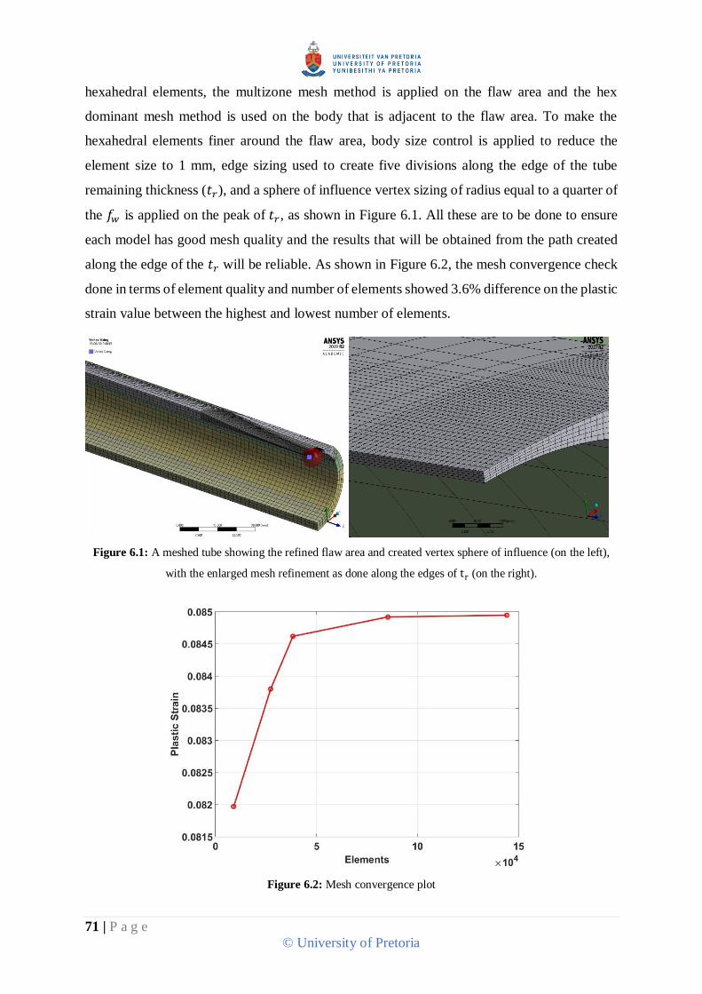
71 | P a g e


hexahedral elements, the multizone mesh method is applied on the flaw area and the hex

dominant mesh method is used on the body that is adjacent to the flaw area. To make the

hexahedral elements finer around the flaw area, body size control is applied to reduce the

element size to 1 mm, edge sizing used to create five divisions along the edge of the tube

remaining thickness (𝑡𝑟), and a sphere of influence vertex sizing of radius equal to a quarter of

the 𝑓𝑤 is applied on the peak of 𝑡𝑟, as shown in Figure 6.1. All these are to be done to ensure

each model has good mesh quality and the results that will be obtained from the path created

along the edge of the 𝑡𝑟 will be reliable. As shown in Figure 6.2, the mesh convergence check

done in terms of element quality and number of elements showed 3.6% difference on the plastic

strain value between the highest and lowest number of elements.

Figure 6.1: A meshed tube showing the refined flaw area and created vertex sphere of influence (on the left),

with the enlarged mesh refinement as done along the edges of tr (on the right).

Figure 6.2: Mesh convergence plot

72 | P a g e


For the boundary conditions, frictionless supports are applied on the symmetrical boundaries

of the models and to prevent rigid body motion, a displacement constraint is applied at the

vertex on the lower tip of the model as shown in Figure 6.3. Each FEM is solved with its

operating pressure (the pressure at which each tube failed in reality), which is applied by

surface effect on the inner part of the model and ramped from zero to the given value. Also, an

axial force based on the internal pressure is applied on the face of the model at the far-left side

as shown in Figure 6.3. This helps to introduce the appropriate axial stress without modeling

end cap effects. The model is solved using the direct solver type in ANSYS Mechanical using

initial and minimum sub-steps of 20 and maximum sub-steps of 1000.

Figure 6.3: One of the localized thinned tubes showing all the boundary conditions applied.

Results and Discussion

Results using the second approach material model

Using the second approach material model (less conservative model), failure evaluation of 160

modelled tubes from 16 different tube grades are assessed based on the maximum equivalent

plastic strain and Von Mises stress produced at the deepest point of the flaw area within each

of the tubes when subjected to their respective operating pressures at which they fail, as shown

in Figure 6.4.

73 | P a g e


Figure 6.4: (a) Maximum equivalent von Mises stress and (b) plastic strain produced at the deepest point of one

of the tubes flaw area.

Figure 6.5 depicts the results of the simulation, and it reveals that the plastic strain response

for the normalized remaining thickness of the tubes (with respect to 𝑡𝑚𝑖𝑛) shows a nearly zero

plastic strain for all the tube grades in the interval 𝑡𝑟 = 0.7 𝑡𝑚𝑖𝑛 up to 𝑡𝑚𝑖𝑛. This indicates how

safe these tubes could be within this range of remaining thickness while in service.

Figure 6.5: Plastic strain and normalized remaining thickness of the tubes based on the second material model

The result also indicates that the BS 3059 360 grades have relatively higher plastic failure

strains as compared to other tubes grades. In fact, tube 1 continues to sustain more strain beyond

30% that is well above the material model true ultimate tensile strain (𝜀𝑡,𝑢𝑡𝑠) of ~22%. The

other tube grades depending on their respective flaw geometries sustain broad range of plastic

74 | P a g e


strains (between 6.75% and 22.88%) before failing. Failure in this context means that the

analysis code fails to converge due to plastic strain localization and subsequent element

inversion. All the tubes exceed a minimum of 5% plastic strain (𝑃5%) before failure, with only

two tube grades failing below 10% plastic strain (𝑃10%). The implication of these results is that

a reasonable plastic strain limit that would be safe for these heat resistant seamless tubes while

in use can be deduced. Some earlier studies on localized thin areas had proposed a 𝑃2% limit,

which gave a conservative estimate of the real plastic collapse pressure for pressurized vessels

[19,59]. It could also be recalled that earlier results reported in Section 4.5 from analyzing

failure pressures of modeled conceptualized tubes based on various failure criteria indicated

𝑃5% or 𝑃7.5% as a safe limit criteria. Thus, a 𝑃5% limit as seen from this outcome from real tubes

is proposed as a more suitable failure criterion with reduced conservatism. Also, depending on

one’s appetite for risk, the criterion may be adjusted as deemed fit for different scenarios. For

instance, if a user chooses to use the 𝑃2%, the allowable remaining tube thickness that could be

considered safe will be 0.4 𝑡𝑚𝑖𝑛, while at 𝑃5%, a reduced tube thickness as low as 0.3 𝑡𝑚𝑖𝑛 is

seen to still be safe. By using the proposed strain limit and measuring the remaining thicknesses

of the tubes while in service, the flawed tubes could be ranked based on the severity of their

flaws, such that only the critical ones are repaired or replaced while others that could still be

safe for continued operation are left for the next planned maintenance of the tubes.

From Figure 6.6 and Figure 6.7, based on the different shades of the plots, the effect of the flaw

geometries on the tubes failure in terms of their 𝑓𝑙 𝑓𝑤⁄ and 𝑓𝑤 𝑓𝑑⁄ aspect ratios respectively can

be seen, with Tube 1 having the largest 𝑓𝑙 𝑓𝑤⁄ but the smallest 𝑓𝑤 𝑓𝑑⁄ . The influence of this

lengthy but narrow flaw is most likely one of the reasons Tube 1 is able to sustain continued

plastic strains beyond its 𝜀𝑡,𝑢𝑡𝑠, as earlier reported. In the same manner, other tube grades (like

Tubes 6, 14 and 16) with fairly large 𝑓𝑙 𝑓𝑤⁄ and small 𝑓𝑤 𝑓𝑑⁄ ratios also sustain large plastic

strains.

It can also be observed that tubes (like Tubes 3, 5, 7, 10, 15) with small 𝑓𝑙 𝑓𝑤⁄ but fairly large

𝑓𝑤 𝑓𝑑⁄ ratios equally sustain large plastic strain before failure. Interestingly, the two

observations demonstrate the influence of lengthy but small width flaws and small but fairly

large width flaws that potentially make these tubes sustain gross plastic strains before failing.

The reason for this is that the flaw geometry creates room for the surrounding material to absorb

some of the plastic strains and consequently helps to reduce the strain concentration produced

within the flaw area of the tubes. Thus, making the tubes to sustain more plastic strains before

they eventually fail.

75 | P a g e


Figure 6.6: Plastic strain and normalized remaining thickness of the tubes with respect to their 𝑓𝑙 𝑓𝑤⁄ aspect

ratios based on the second material model coloured from red to blue – the lines are coloured from red to blue,

where more red indicates a smaller value of 𝑓𝑙 𝑓𝑤⁄ and more blue indicates a larger value.

Figure 6.7: Plastic strain and normalized remaining thickness of the tubes with respect to their 𝑓𝑤 𝑓𝑑⁄ aspect

ratios based on the second material model coloured from red to blue - the lines are coloured from red to blue,

where more red indicates a smaller value of 𝑓𝑤 𝑓𝑑⁄ and more blue indicates a larger value.

76 | P a g e


It can be recalled from the Section 4.4.2 when the effect of 𝑓𝑑 𝑓𝑤⁄ and 𝑓𝑤 𝑓𝑑⁄ ratios on the

failure pressure of the tubes were investigated for cases of conceptualized variants of boiler

tubes under localized erosion flaws, the above findings were found to be true for large aspect

ratios. Hence, this current analysis on real tubes expounds and substantiates the previously

reported findings. It can now be seen that tubes with fairly large 𝑓𝑤 𝑓𝑑⁄ ratios and small

𝑓𝑙 𝑓𝑤⁄ will be able to sustain large plastic strains before failing, likewise tubes with a vice versa

flaw geometry.

Also, the above results reveal that the tubes which failed under 𝑃10% (Tube 12 with the smallest

flaw having the smallest 𝑓𝑙 𝑓𝑤⁄ and a small 𝑓𝑤 𝑓𝑑⁄ and Tube 4 with a mid-range 𝑓𝑙 𝑓𝑤⁄ and

𝑓𝑤 𝑓𝑑⁄ ratios), show the possibility for some tubes to fail in reality at quite low plastic strains.

Hence, these two real life examples present another motivation why a lower bound of 𝑃5%

could be a suitably safe strain limit criterion.

Figure 6.8 shows the peak Von Mises stress normalized with the 𝜎𝑢𝑡𝑠 . It can be seen that the

equivalent Von Mises stresses for all the tube grades at 𝑡𝑚𝑖𝑛 are about 0.3 𝜎𝑢𝑡𝑠 and continue up

until 0.9 𝜎𝑢𝑡𝑠 before any failure occurred. Most of the tubes remain intact beyond the 𝜎𝑢𝑡𝑠, with

only Tube 4 and Tube 12 failing at 0.95 𝜎𝑢𝑡𝑠.

Figure 6.8: Von Mises stress with respect to 𝜎𝑢𝑡𝑠 and normalized remaining thickness of the tubes based on the

second material model

Figure 6.9 also reveals that the equivalent Von Mises stresses normalized with respect to the

true ultimate tensile strength (𝜎𝑡,𝑢𝑡𝑠) shows all the tubes exceeding a minimum of 0.7 𝜎𝑡,𝑢𝑡𝑠.

77 | P a g e


Based on these findings, an equivalent Von Mises stress criterion can be deduced that could be

safe for these heat resistant tubes while in service. Previous studies on external eroded pipes

proposed the 𝜎𝑢𝑡𝑠 as their criteria limit [68,72]. Thus, 0.8 𝜎𝑢𝑡𝑠 as a deduced failure criterion

from the result obtained will be a reasonably safe limit for these tubes.

Figure 6.9: Von Mises stress with respect to 𝜎𝑡,𝑢𝑡𝑠 and normalized remaining thickness of the tubes based on

the second material model

Results using the third approach material model

The results of the assessment performed on the same modelled tubes but using the third

approach material model (conservative model) are presented. The maximum equivalent Von

Mises stress and plastic strain produced at the deepest point of the flaw area within each of the

tube are obtained. Considering the result of the plastic strains for the normalized remaining

thickness in Figure 6.10, it will be observed that for all the tube grades from when 𝑡𝑟 = 0.7 𝑡𝑚𝑖𝑛

to 𝑡𝑚𝑖𝑛, there is almost zero plastic strain. It can be recalled that the same was also seen with

the less conservative model in Section 6.3.1. This reinforces the earlier deduction in Section

6.3.1 that the tubes will be safe within the same range of remaining thickness while in

operation.

The result also shows that except for two of the BS 3059 360 grades that have relatively higher

plastic failure strains (beyond their material model 𝜀𝑡,𝑢𝑡𝑠), the other tube grades depending on

their respective flaw geometries sustain a broad range of plastic strains (between 6.76% and

78 | P a g e


22.35%) before failing. All the tubes exceeds a minimum of 𝑃5% before failure, with only Tube

4 failing below 𝑃10%, which indicates the possibility for a tube to fail at low plastic strain.

These results substantiate the earlier result in Section 6.3.1 that a plastic strain criterion that

could be safe for these tubes while in service can be deduced for either specific grades of tubes

or across all commonly used heat resistant seamless tubes in the power generation industry.

Thus, it is proposed that the lower bound 𝑃5% be used as a failure criterion, which can help

prevent replacing tubes that can still be safe for continued operation.

Figure 6.10: Plastic strain and normalized remaining thickness of the tubes based on the third material model

The influence of flaw geometries on the failure of the tubes in terms of their 𝑓𝑙 𝑓𝑤⁄ and 𝑓𝑤 𝑓𝑑⁄

aspect ratios respectively can be seen in Figure 6.11 and Figure 6.12. Here, it can be noticed

that because of the conservativeness of the third model, in addition to Tube 1 with the

largest 𝑓𝑙 𝑓𝑤⁄ but smallest 𝑓𝑤 𝑓𝑑⁄ (as seen in the case of the less conservative model), Tube 3

which has one of the smallest 𝑓𝑙 𝑓𝑤⁄ but fairly large 𝑓𝑤 𝑓𝑑⁄ continued to sustain large plastic

strains beyond their 𝜀𝑡,𝑢𝑡𝑠. Other tubes with fairly large 𝑓𝑙 𝑓𝑤⁄ and small 𝑓𝑤 𝑓𝑑⁄ ratios (like

Tubes 6 and 16), as well as those with small 𝑓𝑙 𝑓𝑤⁄ but fairly large 𝑓𝑤 𝑓𝑑⁄ (like Tubes 5, 8, 10,

15) ratios sustain relatively large plastic strain before failure, similar to what was observed in

Section 6.3.1. This again demonstrates the effect of a lengthy but small width flaw and a small

but fairly large width flaw that cause these tubes to sustain large plastic strains as explained in

Section 6.3.1.

79 | P a g e


Figure 6.11: Plastic strain and normalized remaining thickness of the tubes with respect to their 𝑓𝑙 𝑓𝑤⁄ aspect

ratios based on the third model coloured from red to blue - the lines are coloured from red to blue, where more

red indicates a smaller value of 𝑓𝑙 𝑓𝑤⁄ and more blue indicates a larger value.

Figure 6.12: Plastic strain and normalized remaining thickness of the tubes with respect to their 𝑓𝑤 𝑓𝑑⁄ aspect

ratios based on the third material model coloured from red to blue - the lines are coloured from red to blue,

where more red indicates a smaller value of 𝑓𝑤 𝑓𝑑 ⁄ and more blue indicates a larger value.

80 | P a g e


Based on the result of the equivalent Von Mises stresses as seen in Figure 6.13, it could be

observed that for all the tube grades, the stresses around the flaw area ranged from about

0.3 𝜎𝑢𝑡𝑠 to 0.9 𝜎𝑢𝑡𝑠 before one or two tubes failed. Most of the tubes continue to survive beyond

the 𝜎𝑢𝑡𝑠, with only Tube 4 and Tube 12 grades failing at 0.84 𝜎𝑢𝑡𝑠 and 0.96 𝜎𝑢𝑡𝑠 respectively.

For the equivalent Von Mises stresses with respect to the true ultimate tensile strength (𝜎𝑡,𝑢𝑡𝑠)

as seen in Figure 6.14, a similar observation shows all the tubes grades exceeding a minimum

of 0.7 𝜎𝑡,𝑢𝑡𝑠 . From all these findings, it is obvious that the result from this third material model

closely correlates with that of the second material model, only with Tube 4 failing quicker

because of the conservativeness of the model. In spite of this, the same earlier proposed

equivalent Von Mises stress criterion of 0.8 𝜎𝑢𝑡𝑠 is still adequate for the conservative model.

This will ensure that the tubes remain safe while in service and also avoid their early

replacement.

Figure 6.13: Von Mises stress with respect to 𝜎𝑢𝑡𝑠 and normalized remaining thickness of the tubes based on

the third material model

81 | P a g e


Figure 6.14: Von Mises stress with respect to 𝜎𝑡,𝑢𝑡𝑠 and normalized remaining thickness of the tubes based on

the third material model

Fitness-for-Service Assessment using the API-ASME FFS Standard

Having considered in detail the assessment of these real tubes, which have also been implicitly

validated since they were determined from the respective pressures at which the tubes failed,

it is still necessary to corroborate the proposed methodology and criteria by comparing them

with the fitness-for-service assessment (FFS) on the tubes using the API-ASME standard

[33,34].

FFS methodology

FFS analysis are performed on the 160 models used in this study. The nonlinear (elastic-plastic)

stress analysis of the API-ASME FFS standard considered as the most accurate method is

employed. In the standard, the concept of Load and Resistance Factor Design (LRFD) is to be

used to determine the global plastic collapse load of the pressurized vessel to ensure its

protection against plastic collapse. For the LRFD, different factored load combinations, based

on the loads the vessel is subjected to, are to be used for the numerical analysis. For the case

of internal pressure as applicable to the study presented in this study, the required factored load

combination is given as:

82 | P a g e


Factored Load for Elastic Plastic Stress Analysis = 𝛽. 𝑃 (6.2)

𝛽 is the load factor coefficient based on the factor applied to the 𝜎𝑢𝑡𝑠 to obtain a design

allowable stress, (the value varies for different construction codes) as seen in Table 6.3. RSFa

is the allowable remaining strength factor which by the standard has a recommended value of

0.9.

The FFS is to be performed using the factored load for the finite element analysis (FEA) and if

convergence is attained, it indicates that the boiler tube being analysed is stable globally under

the applied load. If the FE simulation does not converge, the tube thickness would be modified

(increased) or the applied loads reduced, and the analysis is repeated until convergence is

attained. The highest pressure at which the simulation converges is defined as the plastic

collapse pressure, 𝑃𝑝𝑐 . Note that if the simulation converges using the factored load, then the

actual plastic collapse pressure is not obtained, as it is known that plastic collapse would occur

at a greater pressure than is required by the standard.

It is clear from this discussion that determining the plastic collapse load requires many

simulations which do not converge, and consume a lot of computational resources, making this

a tedious procedure.

Table 6.3: Factored loads used for this study based on construction codes of the boiler tubes and applied loads

Construction Code 𝛽 Factored Load for Global Stability

PD 5500 2.35RSFa 2.12𝑃 EN 13345 2.40RSFa 2.16𝑃

ASME Section VIII, Division 2, prior to the 2007 Edition 3.00RSFa 2.70𝑃 Notes: The PD5500 represents the British specification for unfired, fusion welded pressure vessels, which the BS 3059 tubes fall under. While

the EN 13345 represents the EU Standard for unfired pressure vessels that can also be applicable for both the BS 3059 tubes and the DIN

17175 tubes. The SA 210 A1 tubes fall under the ASME Section VIII codes.

In addition to demonstrating the global stability of the tubes (i.e., protection against plastic

collapse) using the factored loads, the standard requires that the protection against local failure

should be satisfied. This is to be done in terms of a strain limit, if the flaw creates a significant

strain concentration within the tube. To ensure local stability for all the tube grades, an elastic

plastic stress analysis based on the plastic collapse load is to be performed to determine a

limiting triaxial strain, 𝜀𝑙𝑡. This will be compared with the sum of the total equivalent plastic

strain, 𝜀𝑝𝑠 within the flaw area and the forming strain, 𝜀𝑐𝑓 if present in the tubes. But since the

tubes all considered in this study are heat treated, the forming strain is taken as zero according

to the standard. Hence, the 𝜀𝑙𝑡 is only compared with the 𝜀𝑝𝑠.

The strain limit criteria to be satisfied is as follows:

83 | P a g e


𝜀𝑝𝑠 + 𝜀𝑐𝑓 < 𝜀𝑙𝑡 (6.3)

Note for heat treatment tubes, 𝜀𝑐𝑓 = 0. The limiting triaxial strain 𝜀𝑙𝑡 is obtained from

𝜀𝑙𝑡 = 𝜀𝑢 ∗ 𝑒𝑥𝑝 [−(𝛼𝑚𝑓

1+𝑚2) ({

𝜎1+𝜎2+𝜎3

3𝜎𝑒} −

1

3)] , (6.4)

where 𝜀𝑢 is the uniaxial strain limit, 𝛼𝑚𝑓 is the material factor for the multiaxial strain limit, 𝑚2

is the strain hardening exponent, 𝜎1, 𝜎2, 𝜎3 are the principal stresses, and 𝜎𝑒is the equivalent

Von Mises stress within the flaw area.

The computation for 𝜀𝑢 and 𝑚2, as well as the value of 𝛼𝑚𝑓 can be obtained from the standard.

Since the heat resistant seamless tubes studied in this research are ferritic steels, only the details

of these materials are provided in Table 6.4. It should be noted that if the elongation or

reduction in area of a tube is specified, then 𝜀𝑢 would be taken as the maximum value of any

of 𝑚2, elongation, and reduction of area. 𝑅𝑜 is the ratio of the minimum specified yield strength

to the minimum specified tensile strength of the tubes (i.e., 𝑅𝑜 = 𝜎𝑦 𝜎𝑢𝑡𝑠⁄ ), 𝐸𝑜 is the elongation

in percentage and RA is the reduction in area in percentage based on the material specification

of the tube.

Table 6.4: αmf value and details for computing 𝜀𝑢 and 𝑚2 from API-ASME FFS [33]

Material Maximum

Temperature 𝜀𝑢 𝛼𝑚𝑓

𝑚2 Elongation Specified Reduction of Area

Specified

Ferritic steel 480℃ 0.60(1.00 − 𝑅𝑜) 2 ∗ ln [1 +𝐸𝑜100

] ln [100

100 − 𝑅𝐴]

2.2

Comparing the proposed methodology and criteria with FFS

Failure assessment of the localized tubes based on the proposed methodology reported earlier

had been carried out using the operating pressure at which the tubes failed. From the assessment

outcome, a strain and stress limit criteria were deduced, which could be applied to the tubes to

ensure they remain safe for continued operation while avoiding their early replacement.

The proposed failure criteria of 5% plastic strain, 𝑃5% or the equivalent Von Mises stress

criterion of 0.8 𝜎𝑢𝑡𝑠 will now be compared to the outcome of the FFS assessment carried out

on the tubes. As explained in Section 6.4.1, FFS requires changing the tube geometry or applied

load in order for the tube to be globally stable under the required factored load. For the purpose

of this comparison, the tubes are not re-rated, but the plastic collapse pressure 𝑃𝑝𝑐 for each tube

is recorded. The load factor is defined as the ratio of the plastic collapse pressure, 𝑃𝑝𝑐 to the

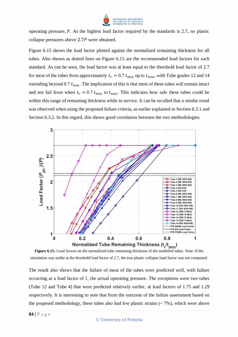
84 | P a g e


operating pressure, 𝑃. As the highest load factor required by the standards is 2.7, no plastic

collapse pressures above 2.7𝑃 were obtained.

Figure 6.15 shows the load factor plotted against the normalized remaining thickness for all

tubes. Also shown as dotted lines on Figure 6.15 are the recommended load factors for each

standard. As can be seen, the load factor was at least equal to the threshold load factor of 2.7

for most of the tubes from approximately 𝑡𝑟 = 0.7 𝑡𝑚𝑖𝑛 up to 𝑡𝑚𝑖𝑛, with Tube grades 12 and 14

extending beyond 0.7 𝑡𝑚𝑖𝑛. The implication of this is that most of these tubes will remain intact

and not fail from when 𝑡𝑟 = 0.7 𝑡𝑚𝑖𝑛 to 𝑡𝑚𝑖𝑛. This indicates how safe these tubes could be

within this range of remaining thickness while in service. It can be recalled that a similar trend

was observed when using the proposed failure criteria, as earlier explained in Section 6.3.1 and

Section 6.3.2. In this regard, this shows good correlation between the two methodologies.

Figure 6.15: Load factors on the normalized tube remaining thickness of the modelled tubes. Note: If the

simulation was stable at the threshold load factor of 2.7, the true plastic collapse load factor was not computed.

The result also shows that the failure of most of the tubes were predicted well, with failure

occurring at a load factor of 1, the actual operating pressure. The exceptions were two tubes

(Tube 12 and Tube 4) that were predicted relatively earlier, at load factors of 1.75 and 1.29

respectively. It is interesting to note that from the outcome of the failure assessment based on

the proposed methodology, these tubes also had low plastic strains (~ 7%), which were above

85 | P a g e


the 𝑃5% limit and failed at about 0.95 𝜎𝑢𝑡𝑠, above the 0.8 𝜎𝑢𝑡𝑠 stress limit. This corroborates

why the proposed plastic strain and stress limit were recommended, leaving allowance for some

uncertainty. A user may still choose a less conservative failure criterion as deemed fit for

different grades of tubes and different scenarios, like in a constrained economic environment

with ageing infrastructures.

However, the FFS failure prediction of all the tubes based on the three recommended load

factors (FFS ASME load factor, FFS EN load factor and FFS PD/BS load factor) occur much

earlier than the operating pressure at which they failed in reality, which is at a load factor of 1.

For instance, based on the FFS PD/BS load factor, which is at 2.12, all the tubes would have

been predicted to be globally unstable and susceptible to plastic collapse below the limit. But

from the result, the tubes continue to survive below that limit up until a load factor of 1. This

shows how conservative the FFS methodology is in predicting the failure of the tubes.

From Sections 2.2.5 and 6.4.1, the use of the FFS actually requires a detailed inspection of the

tube and much information for the assessment. Beyond the 𝜀𝑝𝑠 and 𝜎𝑒, the assessment also

requires the following input: 𝛽 and 𝜀𝑢 ,𝑚2, 𝛼𝑚𝑓, 𝜎1, 𝜎2, 𝜎3 to compute 𝜀𝑙𝑡 for level 3

assessment. The other two lower levels (level 1 and 2) that must be done before level 3

assessment require lot more of input information. Cumbersome FEA simulation is also required

each and every time you need to do an assessment for a particular flaw, which must be

performed by an experienced engineering specialist. All these could be very demanding from

time and cost perspectives.

Based on the challenges of using the FFS, it can be seen that in comparison to the proposed

methodology in this thesis, which involves using the minimum remaining thickness for a

specific tube grade and failure criteria values, given the operating pressure and temperature, a

lot of computation time and resources can be saved and still be able to predict the failure of the

tubes before they occur in reality.

How the Proposed Methodology will be used in Practice

The main requirements to conduct failure assessment on tubes under localized external erosion

using the proposed methodology are the boiler tube grades, the tube and flaw dimensions, and

the operating conditions (temperature and pressure) of the tubes to be assessed. Following the

procedures that have been documented in Chapter 5 and 6, a user can generate the normalized

remaining thickness curves for the plastic strains or normalized equivalent Von-Mises using a

86 | P a g e


set of localized external erosion flaws with the stated requirements. On that basis, they can then

categorize every other detected flaws from the most severe to the least severe, simply by

measuring the remaining tube thickness, 𝑡𝑟, of the tubes based on the proposed failure criteria

of 5% plastic strain, 𝑃5% or the equivalent Von Mises stress criterion of 0.8 𝜎𝑢𝑡𝑠. They may

also choose to adjust the criteria as deem fit to them. By so doing, they will be able to prioritise

the repair or replacement of more critical flawed tubes, judiciously use their maintenance

budget, and ultimately avoid unplanned outages that usually lead to loss of production and

costly emergency repairs.


A failure assessment methodology framework for heat resistant seamless steel boiler tubes with

localized external erosions was presented in this chapter. Flaw geometric properties of these

real failed tubes were obtained and used to accurately replicate the tubes on the already

developed conceptualized geometries. For a detailed failure assessment of the tubes, using the

optimization technique in MATLAB® and through parameterization in ANSYS®, 160 finite

element models with the same tube and flaw dimensions but different remaining thicknesses

(𝑡𝑟) were generated from the 16 tube grades from their initial 𝑡𝑟 to their 𝑡𝑚𝑖𝑛.

Using the MPC material models generated from material data, NLFEA investigations were

conducted on the 160 flawed tubes. These tubes were assessed based on the maximum

equivalent plastic strain and Von Mises stress produced at the deepest point of the flaw area

within each of the tubes when subjected to their respective operating pressures at which they

failed. The following outcomes were established from the failure assessment:

1. The results show a near zero plastic strain response for the normalized remaining

thickness of the tubes (with respect to 𝑡𝑚𝑖𝑛) for all the tube grades from when 𝑡𝑟 = 0.7

𝑡𝑚𝑖𝑛 up to 𝑡𝑚𝑖𝑛. The implication of this is that most of these tubes will remain intact

and not fail from when 𝑡𝑟 = 0.7 𝑡𝑚𝑖𝑛 to 𝑡𝑚𝑖𝑛, which indicates how safe these tubes

could be within this range of remaining thickness while in service.

2. Most of the tube grades sustained a broad range of plastic strains (between 6.75% and

22.88%) before failing, with some even extending beyond 23%. The implication of

these findings is that a reasonable plastic strain limit that could be safe for these heat

resistant seamless tubes while in use can be established. Some earlier studies on

localized thin areas had proposed a 𝑃2% limit, which gave a very conservative estimate

87 | P a g e


of the real plastic collapse pressure for pressurized vessels [19,59]. Thus, a 𝑃5% limit

as seen from this result is an improved failure criterion with reduced conservatism.

3. Tubes with fairly large 𝑓𝑙 𝑓𝑤⁄ and small 𝑓𝑤 𝑓𝑑⁄ aspect ratios and also small 𝑓𝑙 𝑓𝑤⁄ but

fairly large 𝑓𝑤 𝑓𝑑⁄ ratios all sustained large plastic strain before failure. This outcome

demonstrates the influence of lengthy but small width flaws and small but fairly large

width flaws that make these tubes sustain gross plastic strains before failing. The reason

for this is that the flaw geometry creates room for the surrounding material to absorb

some of the plastic strains and consequently helps to reduce the strain concentration

produced within the flaw area of the tubes. This allows the tubes to sustain more plastic

strains before they eventually fail. The possibility for some tubes to fail in reality at

quite low strains was noticed from two tubes that failed below 𝑃10%. Therefore, a lower

bound 𝑃5% limit was recommended as the failure criteria to be used.

4. The equivalent Von Mises stresses for all the tube grades at 𝑡𝑚𝑖𝑛, were about 0.3 𝜎𝑢𝑡𝑠

and continued up until 0.9 𝜎𝑢𝑡𝑠 before any failure occurred. Most of the tube grades

remained intact beyond the 𝜎𝑢𝑡𝑠, with only two tube grades failing at 0.95 𝜎𝑢𝑡𝑠. From

this result, an equivalent Von Mises stress criterion that could be safe for these heat

resistant tubes while in service was deduced as 0.8 𝜎𝑢𝑡𝑠. Previous studies on external

eroded pipes had used the 𝜎𝑢𝑡𝑠 as their criteria limit [68,72], hence, the deduced failure

criterion was considered as a reasonably safe limit for the tubes.

The strain and stress limit criteria deduced from the assessment framework can be employed

to heat resistant seamless tubes to ensure they remain safe for continued operation while

avoiding their early replacement. Even though the assessment results of the real tubes have

been implicitly validated since they were determined from the respective operating pressures

at which the tubes failed, it was still necessary to corroborate the proposed methodology and

criteria by checking and comparing them with the fitness-for-service assessment (FFS) using

the API-ASME standard. The outcomes of the comparison were as follows:

1. The results of the FFS show good correlation between the two methodologies. Similar

to the observations from the proposed methodology, the load factor was at least equal

to the maximum recommended load factor of 2.7 for most of the tubes from

approximately 𝑡𝑟 = 0.7 𝑡𝑚𝑖𝑛 up to 𝑡𝑚𝑖𝑛. This again indicates that most of these tubes

will remain intact and not fail from 𝑡𝑟 = 0.7 𝑡𝑚𝑖𝑛 to 𝑡𝑚𝑖𝑛, establishing how safe these

tubes will be within this range of remaining thickness while in service.

88 | P a g e


2. The result also shows that the failure of most of the tubes were predicted well except

for two tubes that were predicted relatively earlier when compared to their actual failure

pressures. This was similarly observed from the proposed methodology, where the

same tubes also had low plastic strains (~ 7%), which were above the 𝑃5% limit and

failed at about 0.95 𝜎𝑢𝑡𝑠, which was also above the 0.8 𝜎𝑢𝑡𝑠 limit. This corroborates the

choice of the plastic strain and stress limits, which allow room for some uncertainty. A

user may choose to use a less conservative failure criterion as deemed fit for different

grades of tubes and scenarios, such as a constrained economic environment with ageing

infrastructures.

3. However, the FFS failure prediction of all the tubes based on the three recommended

load factors by ASME, BS, and EN occur much earlier than the operating pressure at

which they failed in reality, which was at a load factor of 1. This shows how overly

conservative the FFS methodology is in predicting the failure of the tubes. The FFS

also requires a lot of input for the analysis and a more cumbersome FEA analysis, which

could be very demanding and expensive. Hence, in comparison with the proposed

methodology in this thesis (using the minimum remaining thickness for a specific tube

grade and the failure criteria values, given the operating conditions of the tubes), a lot

of computation time and resources would be saved, and the failure of the tubes would

still be predicted well on time.

The easy-to-use and more efficient failure assessment framework developed will help in

categorizing the severity of localized erosion defects in boiler tubes and consequently support

maintenance decisions, as well as prevent the replacement of tubes that can still be safe for

continued operation while in service. Having developed this failure assessment methodology,

it is also necessary to examine its sensitivity with regards to changes in the flaw geometry and

tube materials. Investigations carried out in this regard and their outcomes are reported in the

next chapter.

89 | P a g e


7 SENSITIVITY STUDY ON THE DEVELOPED METHODOLOGY

Introduction

Although the developed methodology has been validated and demonstrated to be in good

correlation with the established FFS Standard, a sensitivity study is needed to check if changes

in the flaw geometries and material factors could possibly influence the proposed methodology.

In this chapter, a report on how this study is carried out, the outcomes from the study and their

implications will be discussed.

Sensitivity Study Set-Up

Selection of tubes for the study

From the range of the tubes grades used to develop the failure assessment methodology, as

reported in Chapters 5 and 6, five different flawed tubes based on the variation of their flaw

geometries are selected for this study as reported in Table 7.1. The selected tubes reasonably

cover a broad range of scenarios. Figure 7.1 shows the flaw geometries of these flawed tubes.

Table 7.1: Selected localized thinned tubes used for the sensitive study, showing their dimensions, flaw geometric

properties and descriptions

Tubes No

𝐷𝑜 (mm)

𝑡 (mm)

𝑡𝑟

(mm)

𝑓𝑙 (mm)

𝑓𝑤

(mm) 𝑓𝑙 𝑓𝑤⁄ 𝑓𝑤 𝑓𝑑⁄ Flaw Description

1. 75.0 7.0 0.50 600 20 30 3.08 Longest & slender flaw 4. 47.5 5.4 1.20 400 45 8.89 10.71 Fairly large flaw

10. 63.0 5.4 0.42 310 60 5.17 12.05 Widest but short flaw

11. 38.0 3.8 0.45 500 35 14.29 10.45 Mid-range flaw

12. 33.0 3.6 0.20 20 15 4.41 1.33 Smallest flaw

Material properties modification for selected tubes

To carry out the sensitive study with respect to the tubes flaw geometry and material type, the

material properties of all the different tube grades considered in the course of this research will

have to be determined at one specific 𝑇𝑜𝑡 for all the selected tubes, to eliminate any temperature

variation in the material properties. It will be recalled from the previous chapter that these tube

grades were as follows: BS 3059 Grade 360, SA 210 A1, BS 3059 Grade 440, DIN 17175

15Mo3, BS 3059 Grade 360. The specific 𝑇𝑜𝑡 that will be used to conduct this study is at 350℃,

which is a reasonable operating temperature for most heat resistant tubes.

90 | P a g e


From the documentation on how to generate the strength properties of the tubes as a function

of temperature based on the second and third approaches, as seen in Section 5.3.1, the strength

values for each of the tubes based on this new configuration used for the sensitivity study are

shown in Table 7.2. While the physical properties of the tubes at the specific 𝑇𝑜𝑡 are deduced

from Section 5.3.2.

(a) (b)

(c) (d)

(e)

Figure 7.1. Flaw geometries used for the study (a) longest and slender flaw on Tube 1 (b) fairly large flaw on Tube 4 (c) widest but short flaw on Tube 10 (d) mid-range flaw on Tube 11 and (e) smallest flaw on Tube 12.

Table 7.2: Strength properties for selected tubes at specific 𝑇𝑜𝑡

Tube Grades 𝑇𝑜𝑡 (℃)

σy (MPa) at 𝑇𝑜𝑡

computed using Second Approach

σy (MPa) at

𝑇𝑜𝑡 computed using Third Approach

𝜎𝑢𝑡𝑠 (MPa) at


Second Approach

𝜎𝑢𝑡𝑠 (MPa) at 𝑇𝑜𝑡 computed using

Third Approach

BS 3059 Grade 360 350 175.14 124.08 268.30 291.92 SA 210 A1 350 190.04 167.27 309.29 372.24

BS 3059 Grade 440 350 182.59 167.27 327.92 372.24

DIN 17175 15Mo3 350 242.66 165.06 404.43 393.78

BS 3059 Grade 620 350 150.94 160.66 385.74 411.99

91 | P a g e


Material models used for the study

The material models used for the sensitivity study are generated as described in Section 5.4

using the second and third approach strength properties. The plastic region of the developed

stress-strain curves is then implemented in ANSYS® engineering data for static structural

analysis. From the material curves, depicted in Figure 7.2, it is obvious that all of the stress

values (except for the 15 Mo3 grades) based on the second approach strength properties are

relatively less conservative to that of the third approach. As was pointed out in Section 5.4,

using these two models will provide a unique advantage of having a two sided comprehensive

model (one that is conservative and the other less conservative) for a detailed sensitivity

analysis.

Figure 7.2: Material curves for various tube grades at the specific 𝑇𝑜𝑡 based on (a) Second approach and (b)

Third approach strength properties.

Sensitivity Analysis Using the Developed Methodology

To be able to correctly analyze these tubes based on the above stated configuration and using

the developed methodology, the previous P for each of the selected flawed tubes will have to

be modified based on the modified material properties at the specific 𝑇𝑜𝑡. From 𝑡𝑚𝑖𝑛 as seen

in. Eq. (6.1), the modified P can be computed using:

𝑃 = 2.𝑡𝑚𝑖𝑛.𝜎𝑎

𝐷𝑜−𝑡𝑚𝑖𝑛 (7.1)

Obtaining 𝜎 from respective standards of the tube grades and computing 𝑃 for each of the tube,

the complete tube parameters that are used for the sensitivity analysis are shown in Table 7.3.

Finite element models of the selected tubes along with their respective parameterized models

92 | P a g e


(details of the parameterized properties can be seen in Appendix G) are then solved using the

computed 𝑃 on ANSYS® Mechanical platform.

Table 7.3: Selected tubes parameters used for the sensitivity study

Tubes No 𝐷𝑜 (mm) 𝑡𝑚𝑖𝑛 (MPa) Tube Grades 𝜎𝑎(MPa) at 𝑇𝑜𝑡 𝑃 (MPa)

1. 75.0 5.34 BS 3059 Grade 360 87.00 13.34

SA 210 A1 115.42 17.70

BS 3059 Grade 440 106.00 16.25

DIN 17175 15Mo3 120.00 18.40

BS 3059 Grade 620 129.00 19.78

4. 47.5 4.71 BS 3059 Grade 360 87.00 19.15

SA 210 A1 115.42 25.41

BS 3059 Grade 440 106.00 23.34

DIN 17175 15Mo3 120.00 26.42

BS 3059 Grade 620 129.00 28.40

10. 63.0 3.16 BS 3059 Grade 360 87.00 9.19

SA 210 A1 115.42 12.19

BS 3059 Grade 440 106.00 11.20

DIN 17175 15Mo3 120.00 12.67

BS 3059 Grade 620 129.00 13.62

11. 38.0 2.64 BS 3059 Grade 360 87.00 12.99

SA 210 A1 115.42 17.23

BS 3059 Grade 440 106.00 15.83

DIN 17175 15Mo3 120.00 17.92

BS 3059 Grade 620 129.00 19.26

12. 33.0 2.72 BS 3059 Grade 360 87.00 15.63

SA 210 A1 115.42 20.74

BS 3059 Grade 440 106.00 19.04

DIN 17175 15Mo3 120.00 21.56

BS 3059 Grade 620 129.00 23.18

Results and Discussion

Based on the two material models used, the results of the sensitivity study are depicted in Figure

7.3 to Figure 7.6. These figures show that the third approach model is conservative, generally

predicting failure relatively earlier for all the tubes compared to the second approach model, as

expected. Considering the results from the less conservative model in Figure 7.3, it can be seen

that the normalized equivalent Von-Mises stress ratios and plastic strain response for the

normalized remaining thickness of the tubes with respect to 𝑡𝑚𝑖𝑛 do not really change with the

93 | P a g e


assessment result earlier reported in Section 6.3. Using the proposed 𝑃5% limit, failure can be

accurately predicted for all the tubes. Failure as earlier explained means that the analysis code

fails to converge due to plastic strain localization and subsequent element inversion. From

Figure 7.4, it can also be seen that the 0.8 𝜎𝑢𝑡𝑠 proposed criteria is a reasonably safe limit for

these tubes. Thus, it can be seen that in spite of changes in the flaw geometries and tube

materials, the proposed methodology is not affected.

The sensitivity results in Figure 7.3 and Figure 7.4 also reveal that the tubes with DIN 15 M03

tube grades fail at the lowest stress and strain. This is followed by the three BS 3059 tube

grades and the SA 210 tube grades, which though have relatively higher normalized equivalent

stress ratios than other tube grades. But based on the equivalent plastic strains, the BS 3059

620 grade exhibits the highest plastic strains at failure, except for Tube 1, which exceeds the

material model true ultimate tensile strain (𝜀𝑡,𝑢𝑡𝑠), running at high values due to ANSYS

computing capability. The plastic strain difference at failure between the BS 3059 620 and SA

210 grade for all the tubes ranges from ~2.5% to 4%, with Tube 12 at the upper bound, while

no difference is seen with Tube 4. The reason for this is traceable to the strain hardenability of

the grade, even at elevated temperature, as seen from the research on the strength properties of

the tubes in Section 5.3.1. The implication of this result is that for most of the heat resistant

tubes under localized erosion, those with BS 3059 620 grades due to their strain hardenability,

will be able to sustain relatively higher plastic strains compared to their counterpart grades.

Figure 7.3: Plastic strain and normalized remaining thickness sensitivity result based on the second material

model

94 | P a g e


Figure 7.4: Von Mises stress with respect to 𝜎𝑢𝑡𝑠 and normalized remaining thickness sensitivity result based

on the second material model

For the BS 3059 grades of the fairly large and mid-range flawed tubes (Tubes, 4, 10 and 11),

the sensitivity study shows that BS 3059 620 tube grade has the highest normalized stress ratio

and plastic strain, followed by the BS 3059 440 and the BS 3059 360 tube grades. This finding

can be attributed to the material composition of these tube grades. Also referring to the earlier

report from the research on strength properties of the tubes in Section 5.3.1, the BS 3059 360

grade is essentially carbon steel and has the lowest strain hardening capability, while the BS

3059 440 grade, a medium carbon steel and BS 3059 620 grade, an alloyed steel have better

strain hardenability.

The results so far give useful insights into the effect different grades of heat resistant tubes

could pose on the tubes as they deform in service, which will evidently help to provide guidance

with taking proactive measures for the maintenance of the tubes.

Based on the third approach model in Figure 7.5 and Figure 7.6, the results also showed no

appreciable changes with the outcomes of the assessment earlier reported in Section 6.3. Using

the proposed 𝑃5% and 0.8 𝜎𝑢𝑡𝑠, all the tubes are seen to be within the safe limit. This again

shows that proposed methodology is not affected by changes in the geometry of the flaws and

tube materials. The results also indicates that the BS 3059 620 tube grade sustained relatively

higher plastic strains at failure and normalized stress ratios than other tube grades, with the

exception of the BS 3059 360 grade for Tube 1, which exceeds the material model true ultimate

95 | P a g e


tensile strain (𝜀𝑡,𝑢𝑡𝑠), and continued solving at high plastic strain values due to ANSYS

computing capability. It could be recalled from the earlier report based on the less conservative

second approach model, that the BS 3059 620 grade also showed high plastic strain at failure

and stress ratios for most of the tubes. Based on this, the result from this conservative model,

thus, substantiates this finding.

Figure 7.5: Plastic strain and normalized remaining thickness sensitivity result based on the third material

model

Figure 7.6: Von Mises stress with respect to 𝜎𝑢𝑡𝑠 and normalized remaining thickness sensitivity result based

on the third material model

96 | P a g e


Equally, from Figure 7.5 and Figure 7.6, the results of the conservative third approach model,

which has less variation between the material curves demonstrates an improved safety

prediction for the DIN 15 M03 tube grades compared to that seen with the second approach

model. The BS 3059 620 tube grades also have the highest strain and stress ratios before failure

(as also seen with the second approach), followed by the DIN 15 Mo3, the SA210, the BS 3059

360, and the BS 3059 440 tube grades. This outcome can be attributed to the influence of the

conservative model on the strain hardenability of these tubes. Their strain hardenability become

quite conservative when compared to their (engineering strength values or the true stress values

of the less conservative model) at elevated temperature, as seen in Sections 5.3.1 and 5.4.

The distinction between Tube 12 and other flawed tubes is also visibly noticed in all the figures

(Figure 7.3 to Figure 7.6) from the two models used, with the flawed tube still able to sustain

itself at very low tube remaining thickness ratio of ~0.075 though at a lower normalized stress

and strain ratios. The rationale for this is ascribable to the flaw small size, which will first create

substantial strain concentration within the flaw area as the tube deforms while in use. But over

time, the concentration effect reduces, as it become largely absorbed by the substantial elastic

material around the flaw. This ends up reducing the stress and strain ratios within the tube,

while sustaining it in service before it eventually fails at a very low ratio of the tube remaining

thickness. In contrast, other flawed tubes are not able to attain this low ratio, as they all failed

at about 20% of their remaining thicknesses or more. Similar to the results in Chapter 4 and 6,

these findings give further understanding of how sensitive the tubes are to their flaw geometry.

The insights from this sensitivity analysis provides us with a deeper understanding of the

interplay between the various grades of commonly used heat resistant tubes and their failure

under localized external erosion.


This chapter presents the report of the sensitivity study based on the developed methodology

carried out on some carefully selected localized thinned tubes from the set of real flawed tubes

used as case study for this research. Five different flawed tubes based on the variation of their

flaw geometries were selected for this study. The tubes reasonably cover a broad range of

scenarios (from smallest through mid-range flaws to longest and slender flaws). The sensitivity

study was done to examine how the combination of the flaw geometry and material factors

could possibly influence the failure of the tubes while in use, using the developed methodology.

97 | P a g e


For the set-up of this study, the material properties of the five grades (BS 3059 Grade 360, SA

210 A1, BS 3059 Grade 440, DIN 17175 15Mo3, BS 3059 Grade 360) of the tubes were

modified at a fixed operating temperature 𝑇𝑜𝑡 of 350℃ to eliminate the effect of any

temperature variation on the material properties of the selected tubes. The modification of these

properties was carried out using two different approaches, from which two material models

(one that is conservative and the other less conservative) were generated and used for the

sensitivity analysis.

In order to analyze these tubes correctly based on the modified configuration and using the

already developed methodology, the previous P for each of the selected flawed tubes were

modified at the specific 𝑇𝑜𝑡. Finite element models of the selected tubes along with their

respective parameterized models were then solved using the modified 𝑃 in ANSYS®.

Based on the results from the sensitivity study using the two material models, it was seen that

changes in the flaw geometries and tube materials did not really affect the normalized Von-

Mises Stress ratios and plastic strain response for the normalized remaining thickness of the

tubes with respect to 𝑡𝑚𝑖𝑛. The proposed 𝑃5% limit correctly predicted the failure for all the

tubes. The 0.8 𝜎𝑢𝑡𝑠 proposed criteria also was a reasonably safe limit for the tubes.

The results from the second approach model (less conservative model) also indicated that the

DIN 15 M03 tube grades fail at the lowest stress and strain, which was followed by the three

BS 3059 tube grades and the SA 210 tube grades that had relatively higher normalized

equivalent stress ratios than other tube grades. However, the BS 3059 620 grade exhibits the

highest plastic strains at failure. Similarly, the results based on the third approach model

substantiated this finding, as the BS 3059 620 grade sustained relatively higher plastic strains

at failure and normalized equivalent stress ratios than the other tube grades. The reason for this

could be linked to the strain hardenability of the grade, even at elevated temperature. The

implication of this result is that for most heat resistant tubes under localized erosion, those with

BS 3059 620 grades, will be able to sustain relatively higher plastic strains compared to their

counterpart grades due to their improved strain hardenability.

From the less conservative model results of the BS 3059 grades of mid-range and fairly large

flawed tubes, the sensitivity study shows that BS 3059 360 had the lowest normalized stress

ratio and plastic strain, followed by the BS 3059 440 and then the BS 3059 620 grades. This

finding can be attributed to the material composition of these tube grades, in which the BS

3059 360 grades are carbon steel materials and had the lowest strain hardenability, while the

98 | P a g e


BS 3059 440 grades, a medium carbon steel and BS 3059 620, an alloyed steel had better strain

hardenability.

It is also worth mentioning that the results of the third approach model had improved safety

prediction for the DIN 15 M03 tube grades compared to that which was seen with the second

approach model. The BS 3059 620 tube grades, as was seen with the second approach model,

had the highest strain and stress ratios before failure, followed by the DIN 15 Mo3, the SA 210,

the BS 3059 360, and the BS 3059 440 tube grades. The outcome of this result was based on

the effect of the conservative model on the strain hardenability of these tube grades, making

them quite conservative when compared to their engineering strength values or the true stress

values of the second approach model at elevated temperature.

Finally, the distinction between the tube with the smallest flaw and other flawed tubes was

clearly seen from all the results of the two models used, with the tube still able to sustain itself

at very low tube remaining thickness ratio of ~0.075 though at a lower normalized stress and

strain ratio. This was due to the small size of the flaw, which will first create substantial elastic

strain concentration within the flaw area as the tube deforms while in use. But as the load

increases, the effect of this strong elastic stress concentration reduces due to the relatively large

surrounding material around the flaw that remains in the elastic domain. This ultimately

reduces the stress and strain ratios within the tube, while sustaining it in service before it

eventually fails at a very low ratio of the tube remaining thickness. Contrary, other flawed tubes

failed at about 20% of their remaining thicknesses and more. These findings give further

understanding of how sensitive the tubes are to their flaw geometry.

The above results from this study give useful insights into how sensitive the in-service behavior

of an externally eroded tube is when using different grades of heat resistant tubes. They provide

deeper understanding of the interplay around the various grades of commonly used heat

resistant tubes in relation to their failure under localized external erosion. These findings will

help to provide guidance with taking proactive measures for the maintenance of the tubes.

99 | P a g e


8 CONCLUSIONS AND RECOMMENDATIONS

Summary of Thesis

Boiler tubes used in power plants, manufacturing and processing industries usually operate in

an erosive-corrosive and high temperature environment and as such are exposed to a broad

range of failures while in use. One of the most common tube failure mechanisms in these

industries is localized external erosion, wherein the tube undergoes considerable loss of its wall

thickness within a localized area under the influence of some erosive components within the

plant. As time passes, the localized thinning of tube evolves into gross plastic deformation,

leading to the eventual bursting of the tube. This failure has been a leading cause of tube

leakages, availability loss and unscheduled boiler outages in the relevant industries, usually

resulting in loss of production and unplanned expensive repairs.

Even though this problem has received attention over the years, most of the studies on the tubes

have been centered on metallurgical failure investigations, visual inspections, chemical

composition and microstructural analyses to determine the root cause of the failure and in some

cases propose recommendations for preventive measures. A few studies have tried to estimate

to the tube remaining life, while others have proposed guidelines to prevent the erosive particles

from the combustion chamber of the plant from impinging on the tubes. In spite of these efforts,

the problem of localized external erosion in boiler tubes continues to be a leading cause of tube

leakages and unscheduled boiler outages in power plants and other utilities.

The American Petroleum Institute (API) and the American Society of Mechanical Engineers

(ASME) also developed a standard document to provide guidance in conducting fitness-for-

service assessments of pressurized vessels and their components, containing a damage or flaw

while in service. But this has also had its challenges, which includes: the assessment requiring

a detailed inspection and many input details, cumbersome FEA simulations that are needed for

the highest level of assessment, which is only considered as the most reliable for severe flaw

assessment, and also the concept of factored loads used for the assessment that have

possibilities of giving relatively conservative results, which could lead to replacing tubes that

still could continue to be safe for operation.

Based on the aforementioned, there has been, therefore, a need to approach this persistent

problem from a different perspective and engage in further studies that will lead to a rapid

100 | P a g e


decision making tool to assess the flaws and prioritize their repairs or replacement. This is

especially crucial in a constrained economic environment with ageing infrastructure, where one

does not want to replace flawed tubes that could still be safe for continued service, while also

avoiding their unexpected failure and all the already mentioned negative issues associated with

their failure. Therefore, a procedure is required that can rank detected flaws from most likely

to fail to least likely to fail. It is for this reason that a series of detailed studies were performed

and reported in this thesis to provide a pragmatic solution to this problem.

In the first chapter of the thesis, a general background and motivation for the study on localized

external erosion in boiler tubes was reported. The aims and research objectives were clearly

spelt out and the scope of the research was also well defined.

The second chapter gave an account of the literature on this topic, beginning with a review of

the initial studies that led to the development of different failure assessment methodologies and

criteria for pressure vessels. A detailed review of the methodologies and criteria that could

predict the failure of these vessels while in service was presented. In addition, previous

numerical studies on localized external erosion in boiler tubes were reported. The ASME and

API fitness-for-service assessment guides were also discussed and the challenges inherent in

them were discussed. From the literature review, it was evident that though metallurgical

investigations and finite element studies have been done to determine the root cause of these

failures and also provide some preventive measures to avoid their reoccurrence, a focused study

on which flaws in boiler tubes are most at risk of failure due to plastic collapse has not been

done.

Based on this background, it was apparent that more detailed studies were needed to able to

rank detected flaws from most severe to least severe. This would allow operators to optimize

the available budget to focus attention where necessary, reducing the likelihood of unexpected

outages. Thus, the third chapter of this thesis reported on the initial investigation of localized

external eroded tubes, which was the modelling of tubes with variants of conceptualized

localized external flaw geometries that exist in real scenarios. The geometric definitions of

these flaws to aid in the process of replicating real tubes on the conceptualized models was also

discussed.

Chapter Four presented the report on comprehensive studies carried out on the modelled

localized external eroded tubes. The outcome of these investigations provided useful insights

into the factors that influence the failure of these tubes while in use. It was inferred from the

101 | P a g e


studies that beyond the material removal associated with localized external erosion, the elastic

stress concentration and flaw geometry play critical roles in influencing the failure of tubes.

The failure pressures of the modelled tubes were analyzed using a range of failure criteria, to

determine which failure criterion would be best recommended for the failure assessment of the

locally flawed tubes. Based on the result, 7.5% plastic strain or 5% plastic strain criteria were

proposed because they had lower failure pressures that were reasonably safe from the extreme

benchmark failure criterion of 20% plastic strain. These criteria were safer options to guard

against unexpected failures of the tubes, while also trying to avoid being overly conservative

with using the lowest 2% plastic strain criterion.

Insights gained from the studies carried out on conceptualized variants of localized thinned

tubes in Chapter Four were extended to 16 real examples of failed externally eroded tubes

obtained from the power generation industry, representing 5 different tube materials. Chapter

Five reported on the methodology to obtain realistic material properties and models from

design codes. A detailed assessment of the strength and physical properties of a range of

commonly used heat resistant boiler tubes in fossil-fuel industries, operating within high

temperature and pressure environments while in service were carried out. The material

properties for each tube material were used to generate two distinct true stress-strain hardening

material models based on the Material Properties Council (MPC) stress-strain models. This

was to ensure that the effect of strain hardening in the tubes as they deform plastically was

properly captured in the failure assessment. Previous published papers had not taken this into

consideration, and some had used elastic-perfectly plastic models.

The Sixth chapter reported on how the failure assessment was performed. The failed tubes were

treated as an inverse problem and an optimization technique in MATLAB® was used to obtain

the geometric properties of the real flaws to effectively replicate them on the already developed

conceptualized geometries. For a thorough failure assessment of the tubes, 160 finite element

models with the same tube and flaw dimensions but varying remaining thicknesses (𝑡𝑟) were

generated from the 16 tubes. Using the generated MPC material models, comprehensive

Nonlinear Finite Element Analysis (NLFEA) investigations were conducted on the 160

modelled flawed tubes. These tubes were assessed based on the maximum equivalent plastic

strain and Von Mises stress produced at the deepest point of the flaw area within each of the

failed tubes when subjected to their respective operating pressures. The failure assessment

outcome revealed that most of the heat resistant tubes while in service will remain safe if their

remaining thicknesses 𝑡𝑟 are within the range of 0.7 𝑡𝑚𝑖𝑛 to 𝑡𝑚𝑖𝑛. A 5% plastic strain and

102 | P a g e


equivalent Von Mises stress criteria of 0.8 𝜎𝑢𝑡𝑠 were deduced as appropriate failure criteria to

guard against the failure of these tubes while in service, and also avoid their early replacement.

Though the assessment results of these real tubes were already implicitly validated since they

were determined from the respective operating pressures at which the tubes failed, the

developed methodology framework was checked and compared with the API-ASME FFS

standard and found to be in good agreement with it, being also less complex, efficient and less

conservative. The FFS assessment requires pressure vessels to be re-rated for a lower pressure

if they do not comply with the specified load factor, imposing a severe requirement on the

operator. In this analysis, rather than varying the operating pressure, the remaining tube

thickness was varied, and a thickness-based failure criterion was proposed.

Chapter Seven of the thesis reported on a sensitivity study to examine how the combination of

the flaw geometry and material factors could possibly influence the failure of the tubes while

in use, using the developed methodology. This sensitivity study aimed to demonstrate that the

results from Chapter Six are generalizable. This was carried out on five carefully selected

localized thinned tubes from the set of real flawed tubes that were used as case study for this

research. The selected tubes covered a broad range of flaw geometries (from small and deep,

through mid-range flaws to a long and slender flaw). These five flaw geometries were

combined with the five tube materials to generate 25 analyses. The material properties of the

five grades of the tubes used for the study were modified at a fixed operating temperature 𝑇𝑜𝑡

of 350℃ to eliminate the effect of any temperature variation on the material properties of the

selected tubes. Just as in chapter Four, two MPC material models (one that is conservative and

the other less conservative) were used for the sensitivity analysis.The previous operating

pressures P for each of the selected flawed tubes were modified at the specific 𝑇𝑜𝑡. Finite

element models of the selected tubes along with their respective parameterized models were

then solved using the modified 𝑃 in ANSYS®.

From the results of the sensitivity study using the two material models, it was seen that the

normalized stress ratio and the plastic strain response for the normalized remaining thickness

of the tubes with respect to 𝑡𝑚𝑖𝑛, were not remarkably affected by changes in the flaw

geometries and tube materials. The proposed 𝑃5% and 0.8 𝜎𝑢𝑡𝑠 limits accurately predicted the

failure for all the tubes and were reasonably safe limit for the tubes.

The results using the less conservative model (the second approach) also revealed that the DIN

15 Mo3 tube grades fail at the lowest stress ratios and strain, which was followed by the three

103 | P a g e


BS 3059 tube grades and the SA 210 tube grades. The BS 3059 620 tube grade (one of the BS

3059 tube grades) had the highest plastic strain at failure. The outcome of the result showed

that for most of the heat resistant tubes under localized erosion, those made from BS 3059 620

will be able to sustain relatively higher plastic strains compared to their counterparts due to the

higher strain hardenability. The effect of the strain hardenability for the BS 3059 360, 440 and

620 grades of mid-range and fairly large flawed tubes were also apparent. The conservative

results obtained using the third approach material model, which had less variation between the

material curves, accordingly, showed less variation in the stress ratios and strain at failure. The

highest values were observed with the BS 3059 620 material, followed by the DIN 15 Mo3,

the SA 210 and the BS 3059 360 tube grades. The BS 3059 440 tube grades had the lowest

values. Again, this was due to the variations in the strain hardenability of these materials.

The distinction between the tube with the smallest flaw and other flawed tubes was clearly seen

from both results, as the tube was able to sustain itself at very low tube remaining thickness

ratio of ~0.075 though at a lower normalized stress and strain ratios. Other flawed tubes failed

at about 20% of their remaining thicknesses.

In general, the sensitivity study clearly shows that the conclusions from the failure assessments

do not change if we use different geometries or materials. All the above gained insights from

this sensitivity study will help to support maintenance decisions on these tubes while in service.

Conclusions

In this thesis, detailed studies were performed and reported to provide a rapid decision making

tool for assessing and ranking localized external erosion defects in boiler tubes, so as to

prioritize their repairs or replacement.

The outcome of the comprehensive research done provided useful insights into the mechanical

behaviour of localized external erosion flaws and the factors that could possibly influence the

failure of the tubes. Conceptualized variants of localized thinned tubes with geometries that

could realistically occur in practical scenarios were modelled. Previous FEA studies on boiler

tubes were performed with less precise flaw geometries. Also, the insights gained from the

explicit investigations on these factors are useful in providing some guidance in categorizing

detected flaws on tubes while in use from most severe to least severe. This enables proper

planning of which flawed tubes should be repaired or replaced before the next scheduled shut

down of the plant. Consequently, this will help to optimize the available budget and

maintenance resources, and also focus attention where absolutely necessary.

104 | P a g e


A new, easy-to-use and efficient failure assessment methodology framework was developed

from extensive NLFEA investigations carried out on real failed tubes obtained from the power

plant. The failure assessment was conducted by treating the tubes as an inverse problem and

using an optimization technique to obtain the flaw geometric properties of the real tubes so as

to effectively replicate them on the developed conceptualized models. MPC material models

that enabled the effect of strain hardening to be properly captured in the tubes as they deform

were used for the analysis. The developed methodology is distinctive, as previous proposed

methods did not use this approach before nor captured the effect of strain hardening in the tubes

in this reported manner. The assessment outcome led to the establishment of a plastic strain

and stress limit criteria that can be employed to heat resistant seamless tubes to ensure they

remain safe for continued operation, while avoiding their early replacement. The methodology

proposed mainly require a minimum remaining thickness for a specific tube grade, the

operating pressure and temperature to perform a localized external erosion failure assessment

on the fitness-for-service of any tube in operation. The methodology was checked and

compared with the API-ASME fitness-for-service assessment and found to be in good

correlation with it, also easy to use, more efficient and with reduced conservatism.

Sensitivity studies were also conducted based on the developed methodology to examine how

the combination of the flaw geometry and material factors could possibly influence the failure

of the tubes while in use. The study outcome shows that there were no appreciable changes in

the normalized Von-Mises stress ratios and the plastic strain response for the normalized

remaining thickness of the tubes. The proposed 𝑃5% and 0.8 𝜎𝑢𝑡𝑠 limits accurately predicted the

failure for all the tubes and were reasonably safe limit for the tubes. Insights gained from the

strain hardenability of the tubes studied will also help with making timely and suitable

decisions on the maintenance of the tubes.

Finally, the technique that has been developed in this thesis will help to rank detected flaws

from most severe to least severe. So in a constrained economic climate, whatever the

maintenance budget permits, the technique will enable the most severe flaws to be repaired

first. This will hopefully enable the plant to operate until the next planned outage, or at least

maximize the time to failure.

Recommendations

For further implementation of this research, especially for the interest of the power generation

industry, it would be recommended that the developed methodology framework presented in

105 | P a g e


this thesis be configured into an app or a graphical user interface. So that by inputting the tube

and measured flaw geometry, as well as the material properties and operating conditions of the

tubes, the user can get a prompt feedback if the tube can be safe for continued operation or not.

Since this research was focused on providing a rapid decision making tool to aid in prioritizing

the repair and replacement to one of the prevalent problems associated with boiler tubes, there

are still other failures that should be attended to (such as, cracks, corrosion, fatigue, creep, etc.).

Further studies are needed to gain more insights on managing them effectively and also develop

easy-to-use and improved failure assessment methodology for them, just as it has been done

with localized external erosion.

106 | P a g e


References

[1] S. Chaudhuri, Some aspects of metallurgical assessment of boiler tubes — Basic

principles and case studies, Materials Science and Engineering A. 432 (2006) 90–99.

[2] Cleaver-Brooks Inc., Boiler Room Guide, 2013.

[3] A. ZG, Boiler and Vessels; Steam bolier manufacturers in Czech, ZG. (2015).

https://www.zgsteamboiler.com/project/steam-boiler-manufacturer-in-czech.html

(accessed September 14, 2018).

[4] C.B. Clifford, T.P.S. University, EGEE 439 Alternative Fuels from Biomass Sources:

Production of Steam - Fuel, Penn State College of Earth and Mineral Sciences, The J

A Dutton e-Educational Institute. (2018). https://www.e-

education.psu.edu/egee439/node/584 (accessed September 14, 2018).

[5] M.M. Rahman, J. Purbolaksono, J. Ahmad, Root cause failure analysis of a division

wall superheater tube of a coal-fired power station, Engineering Failure Analysis. 17

(2010) 1490–1494.

[6] D.N. French, Metallurgical failures in fossil fired boilers, John Wiley and Sons, Inc.

(1993).

[7] B. Dooley, P.S. Chang, The current state of boiler tube failures in fossil plants,

PowerPlant Chemistry. 2 (2000) 197–203.

[8] S.R. Bamrotwar, V.S. Deshpande, Root cause analysis and economic implication of

boiler tube failures in 210 MW thermal power plant, IOSR Journal of Mechanical and

Civil Engineering. (2014) 6–10.

[9] S.R.K. Dhamangaonkar, M.R. Nandgaonkar, A. Deshmukh, A. Deshmukh, S. Thakur,

Use of cold air velocity test (CAVT) to locate erosion prone zones in pulverized coal

fired utility boiler, in: Proceedings of the World Congress on Engineering, 2011.

[10] K. Zarrabi, Estimation of boiler tube life in presence of corrosion and erosion processes,

International Journal of Pressure Vessels & Piping. 53 (1993) 351–358.

[11] K. Zarrabi, H. Zhang, Creep and plastic collapse lives of scarred boiler tubes, Materials

at High Temperatures. 15 (1998) 389–393.

[12] ASM Handbook Committee, Failure Analysis and Prevention, 2002.

[13] J.F. Drennen, P. Kratina, Guidelines for control and prevention of fly ash erosion in

fossil fired power plants. Final report by EPRI, USA., 1994.

[14] J. Roy-Aikins, Challenges in meeting the electricity needs of South Africa, in:

107 | P a g e


Proceedings of the ASME 2016 Power and Energy Conference, 2016: p.

V001T05A002.

[15] G.P. Sullivan, R. Pugh, A.P. Melendez, W.D. Hunt, Operations and maintenance best

practices: A guide to achieving operational efficiency, 2010.

[16] K. Zarrabi, A comparison of several boiler tube life prediction methods, International

Journal of Pressure Vessels & Piping Vessels & Piping. 58 (1994) 197–201.

[17] S.W. Liu, W.Z. Wang, C.J. Liu, Failure analysis of the boiler water-wall tube, Case

Studies in Engineering Failure Analysis. 9 (2017) 35–39.

[18] M. Suckling, C. Allen, Critical variables in high temperature erosive wear, Wear. 203–

204 (1997) 528–536.

[19] P. Haribhakti, P.B. Joshi, R. Kumar, Failure Investigation of Boiler Tubes: A

Comprehensive Approach, ASM International, 2018.

[20] Electric Power Research Institute (EPRI), Guidelines for control and prevention of fly

ash erosion, 2011.

[21] K. Zarrabi, H. Zhang, Primary stress in scarred boiler tubes, International Journal of

Pressure Vessels and Piping. 65 (1996) 157–161.

[22] M. Suckling, High temperature erosive wear of a boiler tube steel, PhD Thesis,

University of Capetown. (1996) 190.

[23] R.D. Port, H.M. Herro, D. Robert, The Nalco Guide to Boiler Failure Analysis by Nalco

Chemical Company, 1991.

[24] ESKOM, BTFR mechanism short report: TUT/13/005/UCLF, 2012.

[25] F.-J. Chen, C. Yao, Z. Yang, Failure analysis on abnormal wall thinning of heat-transfer

titanium tubes of condensers in nuclear power plant Part II: Erosion and cavitation

corrosion, Engineering Failure Analysis. 37 (2014) 42–52.

[26] A.K. Pramanick, G. Das, S.K. Das, M. Ghosh, Failure investigation of super heater

tubes of coal fired power plant, Case Studies in Engineering Failure Analysis. 9 (2017)

17–26.

[27] J. Ahmad, J. Purbolaksono, L.C. Beng, A.Z. Rashid, A. Khinani, A.A. Ali, Failure

investigation on rear water wall tube of boiler, Engineering Failure Analysis. 16 (2009)

2325–2332.

[28] S.K. Dhua, Metallurgical investigation of failed boiler water-wall tubes received from

a thermal power station, Engineering Failure Analysis. 17 (2010) 1572–1579.

[29] N. Lee, S. Kim, B. Choe, K. Yoon, D. Kwon, Failure analysis of a boiler tube in USC

coal power plant, Engineering Failure Analysis. 16 (2009) 2031–2035.

108 | P a g e


[30] Y. Gong, Z. Yang, J. Yuan, Failure analysis of leakage on titanium tubes within heat

exchangers in a nuclear power plant. Part II : Mechanical degradation, Materials and

Corrosion. 63 (2012) 18–28.

[31] I. Klevtsov, H. Tallermo, T. Bojarinova, A. Dedov, Assessment of remaining life of

superheater austenitic steel tubes in oil shale PF boilers, Oil Shale. 23 (2006) 267–274.

[32] O. Nau, N.I. Rad, G. Baki, B. Raji, B. An, Prediction and prevention of boiler tubing

systems erosion in thermal plant, Tehnicka Dijagnostika. (2010) 3–9.

[33] American Petroleum Institute (API) and the American Society of Mechanical

Engineers (ASME), Fitness-For-Service API 579-1/ASME FFS-1, 2016.

[34] American Society of Mechanical Engineers (ASME), ASME Boiler and Pressure

Vessel Code, Division 2, Section VIII Rules for Construction of Pressure Vessels,

2015.

[35] M.S. Attia, M.M. Megahed, M.A. Darwish, S. Sundram, Assessment of corrosion

damage acceptance criteria in API579-ASME/1 code, International Journal of

Mechanics and Materials in Design. 12 (2016) 141–151.

[36] R. Peters, P. Kuhn, Burst strength of unstiffened pressure cylinders with slits, NACA

TN. 3993 (1957).

[37] E.S. Folias, The stresses in a cylindrical shell containing an axial crack, 1964.

[38] E.S. Folias, An axial crack in a pressurized cylindrical shell, International Journal of

Fracture Mechanics. 1 (1965) 104–113.

[39] A. Duffy, Studies of hydrostatic test levels and defect behavior, Proceedings of

Symposium on Line Pipe Research, AGA. (1965).

[40] R.B. Anderson, T.L. Sullivan, Fracture mechanics of through-cracked cylindrical

pressure vessels, NACA TN. D-3252 (1966).

[41] H. Kihara, K. Ikeda, H. Iwanaga, Brittle fracture initiation of line pipe, Presented at

International Institute of Welding, Delft. (1966).

[42] W. Crichlow, R. Wells, Crack propagation and residual static strength of fatigue-

cracked titanium and steel cylinders, ASTM STP 415, American Society for Testing

and Materials. (1967) 25.

[43] G.T. Hahn, M. Sarrate, A.R. Rosenfield, Criteria for crack extension in cylindrical

pressure vessels, International Journal of Fracture Mechanics. 5 (1969) 187–210.

[44] M. Muscat, D. Mackenzie, R. Hamilton, A work criterion for plastic collapse, 80 (2003)

49–58.

[45] P.M.A. Mackenzie, C.A. Walker, J. Mckelvie, A method for evaluating the mechanical

109 | P a g e


performance of thin-walled titanium tubes, Thin-Walled Structures. 45 (2007) 400–

406.

[46] C.H.A. Townley, G.E. Findlay, M.A. Goodman, P. Stanley, Elastic-Plastic

computations as a basis for design charts for torispherical pressure vessel ends,

Proceedings of the Institution of Mechanical Engineers. 185 63/71 (1971) 869–877.

[47] M. Save, Experimental verification of plastic limit analysis of torispherical and

toriconical heads, Pressure Vessels and Piping: Design Analysis. ASME Vol 1 (1972)

382–416.

[48] The American Society of Mechanical Engineers (ASME), American Society

Mechanical Engineers, New York, NY, USA, ASME Boiler and Pressure Vessel Code;

Section III. Division 1. (1971).

[49] The American Society of Mechanical Engineers (ASME), American Society of

Mechanical Engineers, New York, NY, USA, ASME Boiler and Pressure Vessel Code;

Section III. Division 1. (1974).

[50] ASME, American Society Mechanical Engineers, New York, NY, USA, ASME Boiler

and Pressure Vessel Code; Section III. Division 1. (2007).

[51] J.C. Gerdeen, A critical evaluation of plastic behaviour data and a united definition of

plastic loads for pressure components., WRC Bulletin. 254 (1979).

[52] ANSI-ASME B31G-1984, Manual for determining the remaining strength of corroded

pipelines, American Society of Mechanical Engineers, New York, NY, USA. (1984).

[53] J.F. Kiefner, P.H. Vieth, A modified criterion for evaluating the remaining strength of

corroded pipe, American Gas Association, PR-3-805, 1989.

[54] ANSI-ASME B31G-1991:, Manual for determining the remaining strength of corroded

pipelines, American Society of Mechanical Engineers, New York, NY, USA. (1991).

[55] D.R. Stephens, P. Krishnaswamy, R. Mohan, D. Osage, G.M. Wilkowski, A review of

analysis methods and acceptance criteria for local thinned areas in piping and piping

components, in: Fitness for Adverse Environments in Petroleum and Power Equipment

ASME PVP-Vol. 359, 1997: pp. 55–65.

[56] B.N. Leis, D.R. Stephens, An alternative approach to assess the integrity of corroded

line pipe - Part I : Current status, Proc. of the 7th International Offshore & Polar Eng.

Conf. IV (1997) 624–634.

[57] B.N. Leis, D.R. Stephens, An alternative approach to assess the integrity of corroded

line pipe - Part II : Alternative criterion, Proc. of the 7th International Offshore & Polar

Eng. Conf. IV (1997) 635–641.

110 | P a g e


[58] D.R. Stephens, B.N. Leis, Material and geometry factors controlling failure of

corrosion defects in piping, in: International Pressure Vessels and Piping Conference,

1997.

[59] Recommended Practice, DET NORSKE VERITAS, DNV-RP-F101, Corroded

Pipelines. (2004).

[60] E.Q. Andrade, A.C. Benjamin, Modified method for the assessment of the remaining

strength of corroded pipelines, IBP413-03, Rio Pipeline Conference & Exposition.

(2003).

[61] G. Chell, Application of the CEGB Failure Assessment Procedure, R6, to Surface

Flaws, Fracture Mechanics: Twenty-First Symposium. (2009) 525-525–20.

doi:10.1520/stp19012s.

[62] M. Kanninen, K. Pagalthivarthi, A theoretical analysis for the residual strength of

corroded gas and oil transmission pipelines, in: Proceedings of Symposium on

Corrosion Forms and Control for Infrastructure, 1991.

[63] D. Ritchie, S. Last, Burst criteria of corroded pipelines-defect acceptance criteria,

Proceedings of the EPRG/PRC 10th Biennial Joint Conference. (1995).

[64] J.R. Sims, B.F. Hantz, K.E. Kuehn, A basis for the fitness for service evaluation,

Pressure Vessel Fracture, Fatigue, and Life Managment, ASME PVP. 233 (1992) 51–

58.

[65] B.F. Hantz, J.R. Sims, C.T. Kenyon, T.A. Turbak, Fitness for service: Groove-like local

thin-areas on pressure vessels and storage tanks, Plant Systems/Components Aging

Management, ASME PVP. 252 (1993).

[66] D.-J. Shim, J. Choi, Y. Kim, Failure strength assessment of pipes with local wall

thinning under combined loading based on finite element analyses, Journal of Pressure

Vesssel Technology. 126 (2004) 179–183.

[67] D.-J. Shim, Y.-J. Kim, Y.-J. Kim, Reference stress based approach to predict failure

strength of pipes with local wall thinning under combined loading, Transactions of the

ASME. 127 (2005) 76–83.

[68] G. Fekete, L. Varga, The effect of the width to length ratios of corrosion defects on the

burst pressures of transmission pipelines, Engineering Failure Analysis. 21 (2012) 21–

30.

[69] J.E. Abdalla Filho, R.D. Machado, R.J. Bertin, M.D. Valentini, On the failure pressure

of pipelines containing wall reduction and isolated pit corrosion defects, Computers

and Structures. 132 (2014) 22–33.

111 | P a g e


[70] K.J. Yeom, Y.-K. Lee, K.-H. Oh, W.-S. Kim, Integrity assessment of a corroded API

X70 pipe with a single defect by burst pressure analysis, Engineering Failure Analysis.

57 (2015) 553–561.

[71] J.W. Kim, C.Y. Park, S.H. Lee, Local failure criteria for wall-thinning defect in piping

components based on simulated specimen and real-scale pipe tests, in: 20th

International Conference on Structural Mechanics in Reactor Technology (SMiRT 20),

2009: pp. 1–14.

[72] B. Ma, J. Shuai, D. Liu, K. Xu, Assessment on failure pressure of high strength pipeline

with corrosion defects, Engineering Failure Analysis. 32 (2013) 209–219.

[73] Y. Kim, Y. Lee, W. Kim, K. Oh, The evaluation of failure pressure for corrosion defects

within girth or seam weld in transmission pipelines, in: Proceedings of the Intenational

Pipeline Conf IPC2004-216, 2004: pp. 1–9.

[74] M. Kamaya, T. Suzuki, T. Meshii, Failure pressure of straight pipe with wall thinning

under internal pressure, International Journal of Pressure Vessels and Piping. 85 (2008)

628–634. doi:10.1016/j.ijpvp.2007.11.005.

[75] M. Kamaya, T. Suzuki, T. Meshii, Normalizing the influence of flaw length on failure

pressure of straight pipe with wall-thinning, Nuclear Engineering and Design. 238

(2008) 8–15.

[76] J.B. Choi, B.K. Goo, J.C. Kim, Y.J. Kim, W.S. Kim, Development of limit load

solutions for corroded gas pipelines, International Journal of Pressure Vessels and

Piping. 80 (2003) 121–128.

[77] J. Kiefner, A. Duffy, Summary of research to determine the strength of corroded areas

in line pipe, Public Hearing, US Dept of Transportation. (1971).

[78] M. Ahammed, Prediction of remaining strength of corroded pressurised pipelines,

International Journal of Pressure Vessels & Piping. (1997) 213–217.

[79] M.S.G. Chiodo, C. Ruggieri, Failure assessments of corroded pipelines with axial

defects using stress-based criteria: Numerical studies and verification analyses,

International Journal of Pressure Vessels and Piping. 86 (2009) 164–176.

[80] B. Ma, J. Shuai, J. Wang, K. Han, Analysis on the latest assessment criteria of ASME

B31G-2009 for the remaining strength of corroded pipelines, Journal of Failure

Analysis and Prevention. 11 (2011) 666–671.

[81] K. Zarrabi, Plastic collapse pressures for defected cylindrical vessels, International

Journal of Pressure Vessels & Piping. 60 (1994) 65–69.

[82] T.A. DePadova, J.R. Sims, Fitness for Service - Local thin areas comparison of finite

112 | P a g e


element analysis to physical test results, Fitness-for-Service and Decisions for

Petroleum and Chemical Equipment, ASME PVP. 315 (1995).

[83] J. Kim, Y. Kim, B. Kang, S. Hwang, Finite element analysis for bursting failure

prediction in bulge forming of a seamed tube, Finite Elements in Analysis and Design.

40 (2004) 953–966.

[84] H. Othman, J. Purbolaksono, B. Ahmad, Failure investigation on deformed superheater

tubes, Engineering Failure Analysis. 16 (2009) 329–339.

[85] G. Dini, S. Mahmoud, M. Vaghefi, M. Lotfiani, Computational and experimental

failure analysis of continuous-annealing furnace radiant tubes exposed to excessive

temperature, Engineering Failure Analysis. 15 (2008) 445–457.

[86] J. Purbolaksono, J. Ahmad, A. Khinani, A.A. Ali, A.Z. Rashid, Failure case studies of

SA213-T22 steel tubes of boiler through computer simulations, Journal of Loss

Prevention in the Process Industries. 23 (2010) 98–105.

[87] J. Purbolaksono, Y.W. Hong, S.S.M. Nor, H. Othman, B. Ahmad, Evaluation on

reheater tube failure, Engineering Failure Analysis. 16 (2009) 533–537.

[88] T.L. Anderson, D.A. Osage, API 579: A comprehensive fitness-for-service guide,

International Journal of Pressure Vessels and Piping. 77 (2000) 953–963.

[89] American Petroleum Institute (API), API 579 Recommended practice for Fitness-For-

Service, 2000.


Engineers (ASME), API 579-1/ASME Fitness-For-Service (API 579 Second Edition),

(2007).


Engineers (ASME), Fitness-For-Service Example Problem Manual, API 579-2/ASME

FFS-2, 2009.

[92] MathWorks, Matlab 2015a 8.5 Version, (2015).

[93] M. Hindley, I. Kalu, H. Inglis, S. Kok, Finite element analysis of boiler tubes under

localized thinning, in: Presented at the 10th South African Conference on Computation

and Applied Mechanics (SACAM) on 3rd October, 2016 in Northwest University,

Potchefstroom, South Africa., 2016.

[94] ANSYS® 2019 R2 Academic Research Version, (2019).

[95] H. Koboyashi, T. Ogawa, Evaluation of corroded and artificially flawed vessels, in:

High Presssure Technology at the Dawn of the New Millenium ASME PVP-VOL. 418,

2001: pp. 69–75.

113 | P a g e


[96] D.-J. Shim, Y.-J. Kim, Y.-J. Kim, Reference stress based approach to predict failure

strength of pipes with local wall thinning under combined loading, Journal of Pressure

Vessel Technology. 127 (2005) 76. doi:10.1115/1.1849228.

[97] J.E. Bringas, Handbook of comparative world steel standards, 3rd Ed., ASTM, 2002.

[98] D. Gandy, Carbon steel handbook, Electric Power Research Institute (EPRI), 2007.

[99] British Standards Institution (BSI), BS 3059: Part 2 British Standard on Steel boiler

and superheater tubes, 1990.

[100] British Standards Institution (BSI), Specification for design and manufacture of water-

tube steam generating plant (including superheaters, reheaters and steel tube

economizers) - BS 1113-1999, British Standards Institution, 2000.

[101] British Standards Institution (BSI), BS-EN-10216-Seamless steel tube for pressure

purposes - Part 2, 2002.

[102] American Society of Mechanical Engineers (ASME), ASME Boiler and Pressure

Vessel Code, Section II, Part D: Materials Properties, 2015.

[103] Deutsche Normen, DIN-17175 Seamless tubes of heat-resistant steels, 1979.

[104] TPS Technitube, Boiler tubes, furnace tubes and heat exchanger tubes, TPS Technitube

Rohrenwerke GMBH. (2017).

[105] American Petroleum Institute (API), API STD 530 Calculation of Heater-Tube

Thickness in Petroleum Refineries, 1996.

[106] T.A. Turbak, J.R. Sims, Comparison of local thin area sssessment methodologies, in:

Service Experience and Reliability Improvement: Nuclear, Fossil and Petrochemical

Plants, ASME-PVP 288, 1994: pp. 307–314.

114 | P a g e


To formulate the mathematical expression for the flaw width, 𝑓𝑤 , the point of intersection on

the x-axis of the circle and ellipse need to be determined, the two simultaneous equations

below are considered:

For the circle:

𝑥2 + 𝑦2 = 𝑟𝑜2 (E 1)

For the ellipse:

𝑥2

𝑎2+

(𝑦−𝑧)2

𝑏2= 1 (E 2)

From E 2,

𝑏2𝑥2 + 𝑎2(𝑦 − 𝑧)2 = 𝑎2𝑏2 (E 3)

𝑎2(𝑦 − 𝑧)2 = 𝑎2𝑏2 − 𝑏2𝑥2 (E 4)

(𝑦 − 𝑧)2 =𝑏2(𝑎2−𝑥2)

𝑎2 (E 5)

y =b√(a2−x2)

a+ z (E 6)

Substituting E 6 into E 1;

𝑥2 + (𝑏√(𝑎2−𝑥2)

𝑎+ 𝑧)

2

= 𝑟𝑜2 (E 7)

𝑥2 +𝑏2

𝑎2(𝑎2 − 𝑥2) + 𝑧2 +

2𝑏𝑧

𝑎√(𝑎2 − 𝑥2) = 𝑟𝑜

2 (E 8)

(1 −𝑏2

𝑎2)𝑥2 + 𝑏2 + 𝑧2 +

2𝑏𝑧

𝑎√(𝑎2 − 𝑥2) = 𝑟𝑜

2 (E 9)

(1 −𝑏2

𝑎2)𝑥2 + 𝑏2 + 𝑧2 − 𝑟𝑜

2 = −2𝑏𝑧

𝑎√(𝑎2 − 𝑥2) (E 10)

((1 −𝑏2

𝑎2) 𝑥2 + 𝑏2 + 𝑧2 − 𝑟𝑜

2)

2

= (−2𝑏𝑧

𝑎√(𝑎2 − 𝑥2))

2

(E 11)

(1 −𝑏2

𝑎2)2

𝑥4 + (𝑏2 + 𝑧2 − 𝑟𝑜2)2 + 2(1 −

𝑏2

𝑎2) 𝑥2(𝑏2 + 𝑧2 − 𝑟𝑜

2) =4𝑏2𝑧2

𝑎2(𝑎2 − 𝑥2) (E 12)

115 | P a g e


(1 −𝑏2

𝑎2)2

𝑥4 + [4𝑏2𝑧2

𝑎2+ 2(1 −

𝑏2

𝑎2) (𝑏2 + 𝑧2 − 𝑟𝑜

2)] 𝑥2 + [(𝑏2 + 𝑧2 − 𝑟𝑜2)2 − 4𝑏2𝑧2] = 0 (E 13)

Let 𝑡 = 𝑥2,

𝐴𝑡2 + 𝐵𝑡 + 𝐶 = 0 (E 14)

𝑡 =−𝐵±√(𝐵2−4𝐴𝐶)

2𝐴

(E 15)

𝑥 = √−𝐵±√(𝐵2−4𝐴𝐶)

2𝐴

(E 16)

𝑤ℎ𝑒𝑟𝑒 𝐴 = (1 −𝑏2

𝑎2)2

; 𝐵 =4𝑏2𝑧2

𝑎2+ 2(1 −

𝑏2

𝑎2) (𝑏2 + 𝑧2 − 𝑟𝑜

2); 𝐶 = (𝑏2 + 𝑧2 − 𝑟𝑜2)2 − 𝑏2𝑧2

Recall,

𝑓𝑤 = 2𝑥

Therefore,

𝑓𝑤 = 2.√−4𝑏2𝑧2

𝑎2+2(1−

𝑏2

𝑎2)(𝑏2+𝑧2−𝑟𝑜

2)±√((4𝑏2𝑧2

𝑎2+2(1−

𝑏2

𝑎2)(𝑏2+𝑧2−𝑟𝑜

2))

2

−4(1−𝑏2

𝑎2)2

𝐶=(𝑏2+𝑧2−𝑟𝑜2)2−4𝑏2𝑧2)

2(1−𝑏2

𝑎2)2

116 | P a g e


Optimization Technique Program

clc;clear global format long g

[xopt,fopt]=fminsearch ('FitPipeFnx', [916.68 894.43 29 21])

H1=xopt(1,1); R1=xopt(1,2); a1=xopt(1,3); b1=xopt(1,4);

z1=H1-R1-b1; %% For n-flaws % z1=H1-R1+b1; %% For u-flaws

Dimensions of Tubes Investigated (one at a time) D=75; t=7; t_rem=0.5; % BS 3059 Grade 360 tube_Fly ash erosion % D=50.8; t=4.4; t_rem=0.3; % BS 3059 Grade 360 tube_Fly ash erosion % D=50.8; t=4.4; t_rem=0.17; % BS 3059 Grade 360 tube_Fly ash erosion % D=47.5; t=5.4; t_rem=1.2; % SA 210 A1 tube_Fly ash erosion % D=50.8; t=6.3; t_rem=0.377; % SA 210 A1 tube_Fly ash erosion % D=63.5; t=6.6; t_rem=0.8; % BS 3059 Grade 440 tube_Falling Slag % D=38; t=3.8; t_rem=0.3; % BS 3059 Grade 440 tube_Fly ash erosion % D=38; t=3.8; t_rem=0.3; % BS 3059 Grade 440 tube_Fly ash erosion % D=63.5; t=6.1; t_rem=0.63; % BS 3059 Grade 440 tube_Soot blower erosion % D=63; t=5.4; t_rem=0.42; % BS 3059 Grade 440 tube_Fly ash erosion % D=38; t=3.8; t_rem=0.45; % BS 3059 Grade 440 tube_Fly ash erosion % D=33; t=3.6; t_rem=0.2; % 15 Mo3 tube_Soot blower erosion % D=44.5; t=5.6; t_rem=0.41; % 15 Mo3 tube_Soot blower erosion % D=33.9; t=6.5; t_rem=0.24; % 15 Mo3 tube_Fly ash erosion % D=44.5; t=5.2; t_rem=0.5; % 15 Mo3 tube_Fly ash erosion % D=34.9; t=4.2; t_rem=0.2; % BS 3059 620 tube_Fly ash erosion

f_D=t-t_rem; A1 = (1-(b1.^2./a1.^2)).^2; B1 = ((4.*b1.^2.*z1.^2)./a1.^2)+(2.*(z1.^2+b1.^2-(D/2).^2).*(1-

(b1.^2./a1.^2))); C1 = (z1.^2+b1.^2-(D/2).^2).^2 - 4*b1.^2.*z1.^2;

Width = 2*sqrt((-B1-(sqrt(B1.^2-4*A1.*C1)))./(2.*A1)) % Width of the n-

shaped flaw

% Width = 2*sqrt((-B1+(sqrt(B1.^2-4*A1.*C1)))./(2.*A1)) % Width of the u-

shaped flaw

Length = 2*sqrt((2*R1.*f_D)-((f_D).^2)) % Length of the

flaw (NB:Same for both n-and u-shaped flaws)

% Construction of ellipse_circle geometric plots (front view of the tube) r=D/2; % Outer radius of tube r2=D/2-t; % Inner radius of tube th = linspace(0,2*pi); % linspace for angles for circle th2 = linspace(0,pi,50); % linspace for angles for ellipse xunit = r * cos(th); % x coords for points on outer circle yunit = r * sin(th); % y coords for points on outer circle xunit2 = r2 * cos(th); % x coords for points on inner circle yunit2 = r2 * sin(th); % y coords for points on inner circle

117 | P a g e


figure(111); subplot(211) hold on plot(xunit, yunit,'k', xunit2, yunit2,'k'); axis equal; hold on ellxunit = a1*cos(th2); ellyunit = b1*sin(th2) + z1; % For n-flaws % ellyunit = -b1*sin(th2) + z1; % For u-flaws plot(ellxunit, ellyunit,'b', 'linewidth',2); % axis([-50 50 -100 100]) axis auto; xlabel('a-axis','FontSize',20) ylabel('b-axis','FontSize',20) set(gca,'FontSize',14) grid on box on

% Construction of rectangle-circle geometric plots (side view of the tube) l=1200; % Length of tube pos=[-l/2 -r l D]; figure(111) subplot(212) rectangle('Position',pos) hold on pos1=[-l/2 -r2 l, D-(2*t)]; rectangle('Position',pos1,'LineStyle','--') axis equal Dp=H1-R1; Dp_com=f_D+Dp; th=linspace(0,pi,50); xunit = Length*cos(th); yunit = -f_D*sin(th)+Dp_com; plot(xunit,yunit,'b', 'linewidth',2); xlabel('Tube Length','FontSize',20) ylabel('Tube Diameter','FontSize',20) set(gca,'FontSize',14) grid on hold off

Fit Pipe Function

function[Error]=FitPipeFnx(x) H=x(1); R=x(2); a=x(3); b=x(4);

% Dimensions of Tubes Investigated (one at a time)

D=75; t=7; t_rem=0.5; fl=600; fw=20; % BS 3059 Grade 360 tube_Fly ash

erosion

% D=50.8; t=4.4; t_rem=0.3; fl=80; fw=25; % BS 3059 Grade 360 tube_Fly ash

erosion % D=50.8; t=4.4; t_rem=0.17; fl=70; fw=40; % BS 3059 Grade 360 tube_Fly

ash erosion % D=47.5; t=5.4; t_rem=1.2; fl=400; fw=45; % SA 210 A1 tube_Fly ash

erosion % D=50.8; t=6.3; t_rem=0.377; fl=150; fw=50; % SA 210 A1 tube_Fly ash

erosion

118 | P a g e


% D=63.5; t=6.6; t_rem=0.8; fl=240; fw=30; % BS 3059 Grade 440

tube_Falling Slag % D=38; t=3.8; t_rem=0.3; fl=110; fw=28; % BS 3059 Grade 440 tube_Fly

ash erosion % D=38; t=3.8; t_rem=0.3; fl=155; fw=32; % BS 3059 Grade 440 tube_Fly

ash erosion % D=63.5; t=6.1; t_rem=0.63; fl=600; fw=50; % BS 3059 Grade 440 tube_Soot

blower erosion % D=63; t=5.4; t_rem=0.42; fl=310; fw=60; % BS 3059 Grade 440 tube_Fly

ash erosion % D=38; t=3.8; t_rem=0.45; fl=500; fw=35; % BS 3059 Grade 440 tube_Fly

ash erosion % D=33; t=3.6; t_rem=0.2; fl=20; fw=15; % 15 Mo3 tube_Soot blower

erosion % D=44.5; t=5.6; t_rem=0.41; fl=225; fw=35; % 15 Mo3 tube_Soot blower

erosion % D=33.9; t=6.5; t_rem=0.24; fl=300; fw=30; % 15 Mo3 tube_Fly ash erosion % D=44.5; t=5.2; t_rem=0.5; fl=140; fw=44; % 15 Mo3 tube_Fly ash erosion % D=34.9; t=4.2; t_rem=0.2; fl=300; fw=30; % BS 3059 620 tube_Fly ash

erosion

%%% For the n-shaped FEM % R = H-(z+b); % Sweeping Radius F_D = (D/2)-(H-R); % Flaw Depth % F_D = (D/2)-(z+b); % Flaw Depth

z=H-R-b; A = (1-(b.^2./a.^2)).^2; B = ((4.*b.^2.*z.^2)./a.^2)+(2.*(z.^2+b.^2-(D/2).^2).*(1-(b.^2./a.^2))); C = (z.^2+b.^2-(D/2).^2).^2 - 4*b.^2.*z.^2; F_W_n = 2*sqrt((-B-(sqrt(B.^2-4*A.*C)))./(2.*A)); % Width of the n-

shaped flaw

F_L = 2*sqrt((2*R.*F_D)-((F_D).^2)); % Length of the

flaw (NB:Same for both n-and u-shaped flaws)

%%% For the u-shaped FEM % R = H-(z-b); % Sweeping Radius % F_D = (D/2)-(H-R); % Flaw Depth % % F_D = (D/2)-(z-b); % Flaw Depth

% z=H-R+b; % A2 = (1-(b.^2./a.^2)).^2; % B2 = ((4.*b.^2.*z.^2)./a.^2)+(2.*(z.^2+b.^2-(D/2).^2).*(1-

(b.^2./a.^2))); % C2 = (z.^2+b.^2-(D/2).^2).^2 - 4*b.^2.*z.^2; % F_W_u = 2*sqrt((-B2+(sqrt(B2.^2-4*A2.*C2)))./(2.*A2)); % Width of the

u-shaped flaw

Error=(F_L-fl).^2+(F_W_n-fw).^2+(F_D-(t-t_rem)).^2; %% n-flaw % Error=(F_L-fl).^2+(F_W_u-fw).^2+(F_D-(t-t_rem)).^2; %% u-flaw End

119 | P a g e


Coefficient values obtained from the FFS Standard used for the Second Approach computation

of the minimum specific yield strength (MSYS) values for different steel grades

For C

arb

on

steels (h

avin

g y

ield str

en

gth

<2

75.9

MP

a), w

hich

app

lies for C

arbon

and M

ediu

m C

arbon

Steels as d

escribed

in th

is pap

er,

the co

efficient v

alues to

be u

sed are as fo

llow

s:

T

(Min

)

℃

T (M

ax)

℃

𝐶0

𝐶1

𝐶2

𝐶3

𝐶4

𝐶5

21

593

3.7

9335351E

-2

-1.8

638

59

65E

-3

6.6

94

70

07

9E

-6

-1.8

251

83

78E

-8

2.3

1521177E

-11

-1.2

2947

065E

-14

For S

teel ty

pe w

ith C

-1/2

Mo (C

arb

on

-Moly

bd

en

um

Allo

y S

teel), th

e coefficien

t valu

es to b

e used

are as follo

ws:

T

(Min

)

℃

T

(Max

)

℃

𝐶0

𝐶1

𝐶2

𝐶3

𝐶4

𝐶5

21

593

3.3

8037095E

-2

-1.7

355

43

80E

-3

8.3

26

38

09

7E

-6

-2.1

1471

664E

-8

3.2

9874

954E

-11

-2.6

932950

8E

-14

For S

teel ty

pe w

ith 1

-1/4

Cr-1

/2M

o (C

hrom

ium

-Moly

bd

en

um

Allo

y S

teel), th

e coefficien

t valu

es to b

e used

are as follo

ws:

T

(Min

)

℃

T

(Max

)

℃

𝐶0

𝐶1

𝐶2

𝐶3

𝐶4

𝐶5

21

593

4.3

8110535E

-2

-2.1

715

39

85E

-3

1.2

17

47

82

5E

-5

-3.8

9315

704E

-8

6.4

3532

344E

-11

-4.7

171

4972E

-14

120 | P a g e


Coefficient values obtained from the FFS Standard used for the Second Approach computation

of the minimum specific ultimate tensile strength (MSUTS) values for different steel grades.

For C

arb

on

steels (h

avin

g y

ield stre

ngth

<2

75

.9 M

Pa

), wh

ich ap

plies fo

r Carb

on

and M

ediu

m C

arbon

Steels as d

escribed

in th

is pap

er,

the co

efficient v

alues to

be u

sed are as fo

llow

s:

T

(Min

)

℃

T (M

ax)

℃

𝐶0

𝐶1

𝐶2

𝐶3

𝐶4

𝐶5

21

593

3.5

5835868E

-2

-8.8

753

19

86E

-4

-4.5

210

88

19E

-6

4.6

79

64

163E

-8

-1.0

78820

77E

-10

6.3

87

93289E

-14

For S

teel ty

pe w

ith C

-1/2

Mo (C

arb

on

-Moly

bd

en

um

Allo

y S

teel), th

e coefficien

t valu

es to b

e used

are as follo

ws:

T

(Min

)

℃

T

(Max

)

℃

𝐶0

𝐶1

𝐶2

𝐶3

𝐶4

𝐶5

21

593

5.6

3401650E

-2

-2.5

467

38

55E

-3

4.8

30

29

30

6E

-6

1.4

01

54

69

4E

-8

-3.8

5657189E

-11

1.4

771680

3E

-14

For S

teel ty

pe w

ith 1

-1/4

Cr-1

/2M

o (C

hrom

ium

-Moly

bd

en

um

Allo

y S

teel), th

e coefficien

t valu

es to b

e used

are as follo

ws:

T

(Min

)

℃

T

(Max

)

℃

𝐶0

𝐶1

𝐶2

𝐶3

𝐶4

𝐶5

21

593

3.3

5950169E

-2

-1.5

954

22

67E

-3

4.1

90

28

07

7E

-6

3.2

13

10

030E

-9

-2.1

4741795E

-11

9.8

535068

9E

-15

121 | P a g e


Table of values from API STD 530 used for the Third Approach computation of the minimum

yield and tensile strengths as documented in the FFS Standard.

Steel Type Temperature Limits and

Strength Values at the given

Minimum Temperature

For Computing Yield

Strength (MPa), 𝜎𝑦

For Computing Tensile

Strength (MPa), σuts

Carbon Steel

(Figure 4A in

API STD 530)

A 161

A192

𝑇𝑚𝑖𝑛 = 149℃

𝑇𝑚𝑎𝑥 = 621℃

𝜎𝑦𝑇𝑚𝑖𝑛 = 157 MPa

𝜎𝑢𝑡𝑠𝑇𝑚𝑖𝑛 = 298 MPa

𝐴0

𝐴1

𝐴2

𝐴3

𝐴4

𝐴5

1.6251089

-3.3124966E-3

5.0904910E-6

-3.3374441E-9

4.9690402E-13

0

𝐵0

𝐵1

𝐵2

𝐵3

𝐵4

𝐵5

1.1720989

-2.0580032E-3

7.6239020E-6

-9.9459690E-9

3.7189699E-12

0

Medium Carbon

Steel

(Figure 4B in

API STD 530)

A 53 Gr. B

A 106 Gr. B

A 210 Gr. A1

𝑇𝑚𝑖𝑛 = 149℃

𝑇𝑚𝑎𝑥 = 621℃



𝐴0

𝐴1

𝐴2

𝐴3

𝐴4

𝐴5

1.6434698

-3.5201715E-3

5.8080277E-6

-4.2398160E-9

8.7536764E-13

0

𝐵0

𝐵1

𝐵2

𝐵3

𝐵4

𝐵5

1.1872106

-2.2083065E-3

8.0934859E-6

-1.0510434E-8

3.9529036E-12

0

C-0.5Mo

(Figure 4C in

API STD 530)

A 161 Gr. T1

A 209 Gr. T1

A 335 Gr. P1

𝑇𝑚𝑖𝑛 = 149℃

𝑇𝑚𝑎𝑥 = 621℃



𝐴0

𝐴1

𝐴2

𝐴3

𝐴4

𝐴5

1.0875314

-2.1270293E-4

-4.4780776E-7

8.4688943E-10

-5.6614129E-13

0

𝐵0

𝐵1

𝐵2

𝐵3

𝐵4

𝐵5

-8.3107781E-2

6.7591546E-3

-1.3556423E-5

1.1122871E-8

-3.5429684E-12

0

1.25Cr-0.5Mo

(Figure 4D in

API STD 530)

A 213 Gr. T11

A 335 Gr. P11

A 200 Gr. T11

𝑇𝑚𝑖𝑛 = 149℃

𝑇𝑚𝑎𝑥 = 621℃



𝐴0

𝐴1

𝐴2

𝐴3

𝐴4

𝐴5

1.1345901

-4.8648764E-4

3.9401132E-8

4.2209296E-10

-3.8709072E-13

0

𝐵0

𝐵1

𝐵2

𝐵3

𝐵4

𝐵5

1.7526113

-7.0066393E-3

2.3037863E-5

-3.2685799E-8

2.0963053E-11

-5.2442438E-15

122 | P a g e


The Material Properties Council (MPC) stress-strain curve model used to produce a true

stress-strain hardening curve for the simulation is described as follows:

𝜀𝑡 =𝜎𝑡

𝐸+ 𝛾1 + 𝛾2 (D 1)

where, 𝜀𝑡 is the total true strain (elastic plus plastic); 𝐸 is the Young’s modulus; 𝜎𝑡 is the true

stress

𝛾1 =𝜀1

2(1 − 𝑡𝑎𝑛ℎ[𝐻]) (D 2)

𝛾2 =𝜀2

2(1 + 𝑡𝑎𝑛ℎ[𝐻]) (D 3)

𝜀1 = (𝜎𝑡

𝐴1)

1

𝑚1 (D 4)

𝐴1 =𝜎𝑦(1+𝜀𝑦)

(𝑙𝑛[1+𝜀𝑦])𝑚1 (D 5)

𝑚1 =𝑙𝑛[𝑅𝑜]+(𝜀𝑝+𝜀𝑦)

(𝑙𝑛[𝑙𝑛[1+𝜀𝑝]

𝑙𝑛[1+𝜀𝑦]])

(D 6)

𝜀2 = (𝜎𝑡

𝐴2)

1

𝑚2 (D 7)

𝐴2 =𝜎𝑢𝑡𝑠𝑒𝑥𝑝[𝑚2]

𝑚2𝑚2

(D 8)

𝐻𝑜 =2[𝜎𝑡−(𝜎𝑦+𝐾{𝜎𝑢𝑡𝑠−𝜎𝑦})]

𝐾(𝜎𝑢𝑡𝑠−𝜎𝑦) (D 9)

𝑅𝑜 =𝜎𝑦

𝜎𝑢𝑡𝑠 (D 10)

𝜀𝑦 = 0.002 (D 11)

𝐾 = 1.5𝑅𝑜1.5 − 0.5𝑅𝑜

2.5 − 𝑅𝑜3.5

(D 12)

Where 𝛾1 is the true strain in the micro-strain region of the stress-strain curve

𝛾2 is the true strain in the macro-strain region of the stress-strain curve

𝜀1 is the true plastic strain in the micro-strain region of the stress-strain curve

𝜀2 is the true plastic strain in the macro-strain region of the stress-strain curve

𝜀𝑝 is the stress-strain curve fitting parameter

123 | P a g e


𝜀𝑦 is the 0.2% engineering offset strain

𝑅𝑜 is the ratio of the engineering yield stress to the engineering tensile stress

𝐴1 is the curve fitting constant for the elastic region of the stress-strain curve

𝐴2 is the curve fitting constant for the plastic region of the stress-strain curve

𝑚1 is the curve fitting exponent for the stress-strain curve equal to the true strain at the

proportional limit and the strain hardening coefficient in the large strain region

𝑚2 is the curve fitting exponent for the stress-strain curve equal to the true strain at the true

ultimate stress

𝐻𝑜 is the stress-strain curve fitting parameter

𝜎𝑦 is the yield stress at temperature of interest

𝜎𝑢𝑡𝑠 is the engineering ultimate tensile stress at temperature of interest

𝐾 is the material parameter for the stress-strain curve model

𝜎𝑡 is to be evaluated using:

𝜎𝑡 = (1 + 𝜀)𝜎 (D 13)

Where ε is the engineering strain and σ is the engineering stress

The values of 𝑚2 and 𝜀𝑝 are obtained from the FFS standard. For ferritic steel (which the heat

resistant steels studied in this work fall under), at temperature limit of 480oC, these are given

as:

𝑚2 = 0.60(1− 𝑅𝑜) (D 14)

𝜀𝑝 = 2.0𝐸 − 5 (D 15)

Parameterized models with remaining tube thicknesses evenly divided from initial 𝑡𝑟 to 𝑡𝑚𝑖𝑛

for each tube used for the study. Group Tubes Tube remaining

thicknesses (mm)

𝐻

(mm)

𝑅

(mm)

𝑎

(mm)

𝑏

(mm)

*1. BS 3059 Grade 360 Initial 𝑡𝑟 0.50 6957.333 6926.333 30.013 89.990

BS 3059 Grade 360 𝑡𝑟2 0.69 7165.882 7134.692 40.806 162.400

BS 3059 Grade 360 𝑡𝑟3 0.87 7375.141 7343.771 44.935 190.290

BS 3059 Grade 360 𝑡𝑟4 1.06 7610.333 7578.773 35.096 110.535

BS 3059 Grade 360 𝑡𝑟5 1.24 7847.040 7815.300 40.138 139.600

BS 3059 Grade 360 𝑡𝑟6 1.43 8113.680 8081.750 35.095 101.603

BS 3059 Grade 360 𝑡𝑟7 1.61 8383.600 8351.490 30.035 70.669

BS 3059 Grade 360 𝑡𝑟8 1.98 8999.133 8966.653 38.944 109.216

BS 3059 Grade 360 𝑡𝑟9 3.66 13508.883 13474.723 60.927 146.145

BS 3059 Grade 360 𝑡𝑚𝑖𝑛 5.34 27145.103 27109.263 169.450 173.248


BS 3059 Grade 360 𝑡𝑟2 0.43 224.935 203.505 120.025 125.289

BS 3059 Grade 360 𝑡𝑟3 0.56 231.811 210.251 145.510 149.130

BS 3059 Grade 360 𝑡𝑟4 0.69 239.178 217.488 189.946 194.358

BS 3059 Grade 360 𝑡𝑟5 0.82 247.077 225.257 190.580 135.285

BS 3059 Grade 360 𝑡𝑟6 0.95 255.566 233.616 334.379 230.778

BS 3059 Grade 360 𝑡𝑟7 1.08 264.704 242.624 740.554 219.769

+BS 3059 Grade 360 𝑡𝑟8 1.34 285.31 262.970 57.912 9.702

+BS 3059 Grade 360 𝑡𝑟9 2.39 422.404 399.014 25.548 10.000

+BS 3059 Grade 360 𝑡𝑚𝑖𝑛 3.43 849.657 825.227 24.105 15.995

3. BS 3059 Grade 360 Initial 𝑡𝑟 0.17 168.088 146.911 25.191 14.062

BS 3059 Grade 360 𝑡𝑟2 0.29 172.372 151.082 25.637 15.045

BS 3059 Grade 360 𝑡𝑟3 0.41 176.914 155.504 25.376 14.961

BS 3059 Grade 360 𝑡𝑟4 0.53 181.730 160.200 25.145 14.909

BS 3059 Grade 360 𝑡𝑟5 0.74 190.920 169.180 25.151 15.451

BS 3059 Grade 360 𝑡𝑟6 0.88 197.650 175.770 25.011 15.574

BS 3059 Grade 360 𝑡𝑟7 1.02 204.937 182.917 25.478 16.722

BS 3059 Grade 360 𝑡𝑟8 1.30 221.430 199.130 25.153 16.877

BS 3059 Grade 360 𝑡𝑟9 2.32 318.831 295.511 25.258 19.685

BS 3059 Grade 360 𝑡𝑚𝑖𝑛 3.33 597.294 572.964 25.473 22.781

4. SA 210 A1 Initial 𝑡𝑟 1.20 4783.560 4764.010 24.339 19.308

SA 210 A1 𝑡𝑟2 1.28 4876.052 4856.422 24.355 19.485

SA 210 A1 𝑡𝑟3 1.36 4972.222 4952.512 24.319 19.510

SA 210 A1 𝑡𝑟4 1.44 5072.277 5052.487 24.275 19.509

SA 210 A1 𝑡𝑟5 1.51 5163.199 5143.339 24.244 19.530

SA 210 A1 𝑡𝑟6 1.59 5271.180 5251.240 24.208 19.550

SA 210 A1 𝑡𝑟7 1.67 5383.810 5363.790 24.238 19.767

SA 210 A1 𝑡𝑟8 1.82 5608.555 5588.385 24.264 20.085

SA 210 A1 𝑡𝑟9 3.27 9412.356 9390.736 24.018 21.649

SA 210 A1 𝑡𝑚𝑖𝑛 4.71 29008.912 28985.852 23.827 23.071

5. SA 210 A1 Initial 𝑡𝑟 0.377 497.282 477.805 25.692 19.475

SA 210 A1 𝑡𝑟2 0.53 509.955 490.325 25.602 19.842

125 | P a g e


SA 210 A1 𝑡𝑟3 0.68 523.035 503.255 25.669 19.773

SA 210 A1 𝑡𝑟4 0.87 540.644 520.674 25.655 19.961

SA 210 A1 𝑡𝑟5 1.06 559.522 539.362 25.641 20.146

SA 210 A1 𝑡𝑟6 1.23 577.600 557.270 25.569 20.518

SA 210 A1 𝑡𝑟7 1.40 596.933 576.433 25.622 20.496

SA 210 A1 𝑡𝑟8 1.74 639.900 619.060 25.601 20.839

SA 210 A1 𝑡𝑟9 3.15 916.682 894.432 25.524 22.245

SA 210 A1 𝑡𝑚𝑖𝑛 4.27 1409.852 1386.482 25.474 23.372


BS 3059 Grade 440 𝑡𝑟2 1.05 1326.300 1300.100 70.027 76.827

BS 3059 Grade 440 𝑡𝑟3 1.29 1385.030 1358.590 101.015 139.202

BS 3059 Grade 440 𝑡𝑟4 1.54 1452.145 1425.455 116.735 156.002

BS 3059 Grade 440 𝑡𝑟5 1.78 1523.116 1496.186 135.675 171.809

BS 3059 Grade 440 𝑡𝑟6 2.03 1604.957 1577.777 150.673 161.694

BS 3059 Grade 440 𝑡𝑟7 2.27 1692.400 1664.980 218.230 238.160

BS 3059 Grade 440 𝑡𝑟8 2.75 1900.000 1872.100 390.189 112.627

+BS 3059 Grade 440 𝑡𝑟9 4.30 3161.034 3131.584 44.804 25.415

+BS 3059 Grade 440 𝑡𝑚𝑖𝑛 5.85 9631.375 9600.375 32.761 27.184


BS 3059 Grade 440 𝑡𝑟2 0.47 471.555 455.885 20.997 11.089

BS 3059 Grade 440 𝑡𝑟3 0.64 496.055 480.215 20.418 11.007

BS 3059 Grade 440 𝑡𝑟4 0.81 523.355 507.345 19.981 11.046

BS 3059 Grade 440 𝑡𝑟5 0.97 552.030 535.860 19.549 11.007

BS 3059 Grade 440 𝑡𝑟6 1.14 586.258 569.918 19.155 11.007

BS 3059 Grade 440 𝑡𝑟7 1.30 622.766 606.266 19.003 11.287

BS 3059 Grade 440 𝑡𝑟8 1.63 714.922 698.092 20.627 15.003

BS 3059 Grade 440 𝑡𝑟9 2.50 1181.811 1164.111 19.515 16.005

BS 3059 Grade 440 𝑡𝑚𝑖𝑛 3.36 3456.282 3437.722 19.373 18.504


BS 3059 Grade 440 𝑡𝑟2 0.47 919.160 903.490 20.791 15.004

BS 3059 Grade 440 𝑡𝑟3 0.64 967.777 951.937 20.543 15.0025

BS 3059 Grade 440 𝑡𝑟4 0.81 1021.907 1005.897 20.311 15.007

BS 3059 Grade 440 𝑡𝑟5 0.97 1078.785 1062.615 20.075 14.956

BS 3059 Grade 440 𝑡𝑟6 1.14 1146.633 1130.293 20.068 15.371

BS 3059 Grade 440 𝑡𝑟7 1.30 1219.000 1202.500 20 15.632

BS 3059 Grade 440 𝑡𝑟8 1.63 1401.840 1385.010 19.855 16.1405

BS 3059 Grade 440 𝑡𝑟9 2.50 2328.446 2310.746 19.223 16.721

BS 3059 Grade 440 𝑡𝑚𝑖𝑛 3.36 6844.064 6825.504 19.031 18.129


BS 3059 Grade 440 𝑡𝑟2 0.75 8440.330 8413.930 31.524 17.470

BS 3059 Grade 440 𝑡𝑟3 0.87 8633.283 8606.763 29.969 15.491

BS 3059 Grade 440 𝑡𝑟4 0.99 8835.399 8808.759 29.969 15.758

BS 3059 Grade 440 𝑡𝑟5 1.10 9029.275 9002.525 30.060 16.140

BS 3059 Grade 440 𝑡𝑟6 1.22 9250.681 9223.811 30.120 16.502

BS 3059 Grade 440 𝑡𝑟7 1.34 9483.205 9456.215 30.011 16.604

BS 3059 Grade 440 𝑡𝑟8 1.57 9963.253 9936.033 31.939 20.251

BS 3059 Grade 440 𝑡𝑟9 2.44 12325.001 12296.911 31.148 21.110

126 | P a g e


BS 3059 Grade 440 𝑡𝑚𝑖𝑛 3.30 16101.778 16072.828 31.496 23.938


BS 3059 Grade 440 𝑡𝑟2 0.55 2505.883 2479.233 32.082 26.769

BS 3059 Grade 440 𝑡𝑟3 0.68 2574.168 2547.388 32.043 26.925

BS 3059 Grade 440 𝑡𝑟4 0.81 2646.307 2619.397 32.025 27.049

BS 3059 Grade 440 𝑡𝑟5 0.93 2716.625 2689.595 32.006 27.168

BS 3059 Grade 440 𝑡𝑟6 1.06 2797.187 2770.027 32.058 27.182

BS 3059 Grade 440 𝑡𝑟7 1.19 2882.722 2855.432 31.884 27.561

BS 3059 Grade 440 𝑡𝑟8 1.44 3062.973 3035.433 31.980 27.588

BS 3059 Grade 440 𝑡𝑟9 2.30 3904.955 3876.555 31.871 28.413

BS 3059 Grade 440 𝑡𝑚𝑖𝑛 3.16 5393.103 5363.843 31.756 29.267


BS 3059 Grade 440 𝑡𝑟2 0.59 9752.580 9736.790 19.506 15.029

BS 3059 Grade 440 𝑡𝑟3 0.73 10196.861 10180.931 19.485 15.2265

BS 3059 Grade 440 𝑡𝑟4 0.87 10683.384 10667.314 19.463 15.4185

BS 3059 Grade 440 𝑡𝑟5 1.01 11217.530 11201.320 19.357 15.387

BS 3059 Grade 440 𝑡𝑟6 1.15 11811.245 11794.895 19.247 15.335

BS 3059 Grade 440 𝑡𝑟7 1.29 12467.944 12451.454 19.198 15.439

BS 3059 Grade 440 𝑡𝑟8 1.55 13906.760 13890.010 19.218 15.937

BS 3059 Grade 440 𝑡𝑟9 2.10 18400.502 18383.202 19.140 16.640

BS 3059 Grade 440 𝑡𝑚𝑖𝑛 2.64 26958.075 26940.235 19.229 17.830

*12. DIN 17175 15Mo3 Initial 𝑡𝑟 0.20 29.506 16.406 10.789 14.325

DIN 17175 15Mo3 𝑡𝑟2 0.34 30.207 16.967 10.613 14.8315

DIN 17175 15Mo3 𝑡𝑟3 0.47 30.909 17.539 10.054 15.105

DIN 17175 15Mo3 𝑡𝑟4 0.61 31.727 18.217 9.915 15.808

DIN 17175 15Mo3 𝑡𝑟5 0.74 32.553 18.913 9.731 16.547

DIN 17175 15Mo3 𝑡𝑟6 0.88 33.522 19.742 9.061 17.1095

DIN 17175 15Mo3 𝑡𝑟7 1.01 34.512 20.600 8.814 18.1585

DIN 17175 15Mo3 𝑡𝑟8 1.28 36.892 22.712 7.242 20.214

+DIN 17175 15Mo3 𝑡𝑟9 2.00 46.950 32.050 37.364 9.977

+DIN 17175 15Mo3 𝑡𝑚𝑖𝑛 2.72 72.878 57.258 18.013 10.165

13. DIN 17175 15Mo3 Initial 𝑡𝑟 0.41 1238.950 1221.890 25.593 12.279

DIN 17175 15Mo3 𝑡𝑟2 0.58 1280.320 1263.090 24.706 11.863

DIN 17175 15Mo3 𝑡𝑟3 0.76 1327.294 1309.884 25.165 13.039

DIN 17175 15Mo3 𝑡𝑟4 0.94 1377.870 1360.280 26.156 14.989

DIN 17175 15Mo3 𝑡𝑟5 1.11 1429.357 1411.597 25.730 15.057

DIN 17175 15Mo3 𝑡𝑟6 1.28 1484.830 1466.900 25.270 15.035

DIN 17175 15Mo3 𝑡𝑟7 1.46 1548.678 1530.568 24.987 15.264

DIN 17175 15Mo3 𝑡𝑟8 1.80 1685.640 1667.190 24.649 15.921

DIN 17175 15Mo3 𝑡𝑟9 2.77 2256.921 2237.501 23.586 17.232

DIN 17175 15Mo3 𝑡𝑚𝑖𝑛 3.74 3423.537 3403.147 22.812 18.546

14. DIN 17175 15Mo3 Initial 𝑡𝑟 0.24 1810.950 1800.260 22.227 10.672

DIN 17175 15Mo3 𝑡𝑟2 0.36 1846.058 1835.248 21.172 9.912

DIN 17175 15Mo3 𝑡𝑟3 0.48 1882.680 1871.750 20.914 10.016

DIN 17175 15Mo3 𝑡𝑟4 0.61 1924.020 1912.960 20.580 10.042

DIN 17175 15Mo3 𝑡𝑟5 0.73 1963.805 1952.625 18.624 8.071

DIN 17175 15Mo3 𝑡𝑟6 0.85 2005.275 1993.975 19.593 9.552

127 | P a g e


DIN 17175 15Mo3 𝑡𝑟7 0.98 2052.233 2040.803 20.445 11.036

DIN 17175 15Mo3 𝑡𝑟8 1.22 2144.990 2133.320 18.926 9.6775

DIN 17175 15Mo3 𝑡𝑟9 1.91 2465.635 2453.275 18.106 10.153

DIN 17175 15Mo3 𝑡𝑚𝑖𝑛 2.60 2899.615 2886.565 18.560 12.544

15. DIN 17175 15Mo3 Initial 𝑡𝑟 0.50 541.180 523.630 22.403 17.561

DIN 17175 15Mo3 𝑡𝑟2 0.64 557.256 539.566 22.378 17.766

DIN 17175 15Mo3 𝑡𝑟3 0.77 573.088 555.268 22.363 17.929

DIN 17175 15Mo3 𝑡𝑟4 0.91 591.204 573.244 22.365 18.041

DIN 17175 15Mo3 𝑡𝑟5 1.04 609.111 591.021 22.378 18.102

DIN 17175 15Mo3 𝑡𝑟6 1.18 629.699 611.469 22.371 18.249

DIN 17175 15Mo3 𝑡𝑟7 1.32 651.750 633.380 22.364 18.391

DIN 17175 15Mo3 𝑡𝑟8 1.57 695.360 676.740 22.360 18.620

DIN 17175 15Mo3 𝑡𝑟9 2.46 915.040 895.530 22.326 19.505

DIN 17175 15Mo3 𝑡𝑚𝑖𝑛 2.80 1041.883 1022.033 22.315 19.847


BS 3059 Grade 620 𝑡𝑟2 0.32 2914.990 2901.420 19.871 11.129

BS 3059 Grade 620 𝑡𝑟3 0.45 3015.590 3001.890 19.032 13.580

BS 3059 Grade 620 𝑡𝑟4 0.57 3114.790 3100.970 19.155 14.000

BS 3059 Grade 620 𝑡𝑟5 0.69 3220.830 3206.890 19.307 14.018

BS 3059 Grade 620 𝑡𝑟6 0.81 3334.320 3320.260 19.123 14.026

BS 3059 Grade 620 𝑡𝑟7 0.93 3456.200 3442.020 18.653 13.545

BS 3059 Grade 620 𝑡𝑟8 1.17 3728.800 3714.380 18.360 12.979

BS 3059 Grade 620 𝑡𝑟9 1.44 4092.150 4077.460 18.039 12.999

BS 3059 Grade 620 𝑡𝑚𝑖𝑛 1.71 4534.277 4519.317 18.211 12.988

*These are the u-shaped flawed tubes, while others are the n-shaped flawed tubes

+These u-shaped flawed tubes initially had n-shaped geometry from 𝑡𝑚𝑖𝑛 to the marked 𝑡𝑟𝑠 but later transitioned

to a u-shaped configuration for the other unmarked 𝑡𝑟𝑠 .

failure assessment of boiler tubes under localized

Documents