factors affecting di stribution of adult … filefactors affecting di stribution of adult yellowfin...

WPTT01-10 IOTC Proceedings no. 4 (2001) page 336 -389

336

FACTORS AFFECTING DISTRIBUTION OF ADULT YELLOWFIN TUNA (THUNNUS ALBACARES) AND ITS REPRODUCTIVE ECOLOGY IN THE INDIAN OCEAN

BASED ON JAPANESE TUNA LONGLINE FISHERIES AND SURVEY INFORMATION

Inter-university Postgraduate Programme in Ecological Marine Management Faculty of Science

Thesis submitted in partial fulfillment for the degree of Master of Science in Ecological Marine Management

ABSTRACT

Environmental influence on yellowfin tuna (Thunnus albacares) distribution and reproductive ecology was analyzed using long line fisheries and oceanographic data in the Indian Ocean for the period of 1953 – 1997. Data were obtained from National Research Institute of Far Seas Fisheries and the National Oceanographic Data Center, respectively. Hooking rates, sexual maturity and larval density were compared with thermocline depth and depth-specific data on temperature, salinity, oxygen and nutrients using geographic information system (GIS) application and simple numerical analyses in order to describe their relationships. Results predicted optimum range for every environmental parameter at each respective life stages of yellowfin tuna. It was found out that water temperature, dissolved oxygen concentration and thermocline depth influenced the distribution of adult yellowfin tuna while, temperature and dissolve oxygen concentration influenced spawning activities. For the larvae, temperature, dissolved oxygen and thermocline depth were also considered important factors. Other environmental parameters studied had more influence on intermediary factors that affects the distribution as well.

ACKNOWLEDGEMENT

I want to start by expressing sincere gratitude to everyone who deserved to be included but was left out unintentionally. They are friends, colleagues, teachers and others who helped me in any way they could.

I would like to express my utmost gratitude to my promoter, Dr. Tom Nishida, for all the efforts he made to make this study possible in spite of the distance between us. Nothing could replace what he did for me. Domo arigato gozaimazu, Nishida-san.

I would also like to extend my thanks to people who willingly helped me during my stay in Japan especially Dr. Kiyoshi Itoh for guiding me on Marine Explorer 3.07 (marine GIS software) and Associate Prof. Masahiko Mohri (National Fisheries University, Shimonoseki) for providing special assistance on the subject matter. . Thanks also to the following scientists of the National Research Institute of the Far Seas Fisheries (including former staff), who assisted my trip to Japan and my study: Yasuhiko Simadzu, Kiyoshi Wakabayashi, Ziro Suzuki, Naizumi Miyabe, Denzo Inagake, Makoto Okazaki, Shyoji Ueyanagi, Yasuo Nishikawa, and Toshio Shiohama. Cheers to the people who made our acquaintances enjoyable even for a short while.

Special thanks to my co-promotor, Dr. Micky Tackx and to Prof. Marie -Hermande Daro for their professional and administrative support to make this thing happen. Thanks also to Ms. Christine Van De Wiele, Patrick Verraes and to my funding agency, Belgian Administration for Development Cooperation.

Thanks to my classmates who shared their insights and help especially David Gillikin who had been assisting me in my review. Thanks, man!

Thanks to my friends who were always there for me to share joy, hopes, encouragement and grief during this ordeal of education in Belgium. I would like to mention them one by one ‘coz who knows when and where we will meet again. They are Georgina Lacastesantos, Leah & Ariel Boven, Cecilia Borromeo, Oliva Idago, Lenny & Allan Ortega, Cristito Andales, Jo-Ann Muriel, Ada Almalvez, Paul Obade, Esther Mwangi, Yusuph Kajia, Anouk Verheyden, Dickson Misate, and the rest.

Last but not the least, I give thanks and love to my family and Luz.

Promotor: Tom Nishida, Ph.D. Research Coordinator of International Resources Management

National Research Institute of Far Seas Fsiheries, Japan

Co-promotor: Prof. Michele Tackx, Ph.D. Department of Biology Vrije Universiteit Brussel, Belgium

cccxliii

Table of Contents

Abstract ...................................................................................................................................................... 342

Acknowledgement ..................................................................................................................................... 342

Table of Contents................................ ................................ ................................ ................................ . cccxliii

List of Tables.........................................................................................................................................cccxliv

List of Figures .......................................................................................................................................cccxliv

List of GIS Maps.................................................................................................................................... cccxlv

1. Introduction.......................................................................................................................................... 1

2. Review ................................................................................................................................................... 1

2.1. BIOLOGY AND ECOLOGY................................................................................................................ 1 (1) Taxonomic description (Bonnaterre, 1788) ..................................................................................... 1 (2) Morphological Characteristics ........................................................................................................ 1 (3) Growth ............................................................................................................................................. 1 (4) Spawning and mode of reproduction ............................................................................................... 1 (5) Larval stage................................ ................................ ................................ ................................ ...... 2 (6) Feeding............................................................................................................................................. 2 (7) Physio logical adaptations................................................................................................................ 2 (8) Distribution................................ ................................ ................................ ................................ ...... 3

2.2. FISHERIES ..................................................................................................................................... 3 (1) General............................................................................................................................................. 3 (2) Longline fisheries ............................................................................................................................. 4

2.3. MARINE ENVIRONMENT................................ ................................ ................................ ................. 4 2.4. PREVIOUS STUDIES........................................................................................................................ 8

3. Information .......................................................................................................................................... 8

3.1. COMMERCIAL TUNA LONGLINE FISHERIES DATA. ................................ ................................ ........... 8 3.2. GONAD DATA................................................................................................................................ 8 3.3. LARVAL DATA ............................................................................................................................... 8 3.4. ENVIRONMENTAL DATA ................................................................................................................ 9

4. Methods ................................................................................................................................................ 9

4.1. DATA PREPARATION................................ ................................ ................................ ...................... 9 4.2. QUALITATIVE ANALYSES USING THE GEOGRAPHIC INFORMATION SYSTEM (GIS) .......................... 9 4.3. NUMERICAL ANALYSES................................ ................................ ................................ ...............11

5. Results.................................................................................................................................................12

5.1. QUALITATIVE ANALYSES USING GIS...........................................................................................12 (1) Hooking rates vs. Environmental factors.......................................................................................12 (2) Spawning activity vs. Environmental factors .................................................................................18 (3) Larval occurrence vs. Environmental factors................................................................................26

5.2. NUMERICAL ANALYSES................................ ................................ ................................ ...............34 (1) Hooking rates vs. Environmental factors (Fig. 10) .......................................................................34 (2) Spawning activities vs. Environmental factors (Fig. 12)................................ ...............................37 (3) Larval distribution vs. Environmental factors (Fig . 13)................................................................37 (4) Spectra of optimum rage of Environmental factors.......................................................................37

6. Discussion...........................................................................................................................................42

6.1. D ISTRIBUTION OF ADULT YFT ................................ ................................ ................................ ....42 6.2. SPAWNING ACTIVITIES.................................................................................................................43 6.3. LARVAL OCCURRENCE ................................................................................................................45 6.4. MIGRATION .................................................................................................................................45

7. Conclusion..........................................................................................................................................46

References................................ ................................ ................................ ................................ ....................47

Appendices ........................................................................................................Error! Bookmark not defined.

cccxliv

List of Tables TABLE 1. SUMMARY OF INFORMATION AND DEFINITIONS OF VARIABLES. ................................ ................................ ....9

TABLE 2. SPECIFICATION OF THE GIS THEMATIC MAPS TO INVESTIGATE SPATIAL CO RRELATION BETWEEN 3 DEPENDENT AND 5 INDEPENDENT

VARIABLES. ...............................................................................................................................................11

TABLE 3. SPECIFICATIONS OF THE GRAPHS (PLOTS) FOR THE NUMERICAL A NALYSES. ................................................12

TABLE 4. OPTIMUM RANGE OF OCEANOGRAPHIC PARAMETERS THAT PRODUCE FAVORABLE HOOKING RATES, SPAWNING ACTIVITIES AND

LARVAE DISTRIBUTION................................. ................................ ................................ .............................40

List of Figures

FIGURE 1. ILLUSTRATION OF A YELLOWFIN TUNA (THUNNUS ALBACARES) .............................................. 1

FIGURE 2. ILLUSTRATI ON ON THE TWO TYPES OF JAPANESE LONGLINE FISHING GEAR COMMONLY U SED. (ADAPTED FROM

MOHRI, 1998). ...................................................................................................................... 4

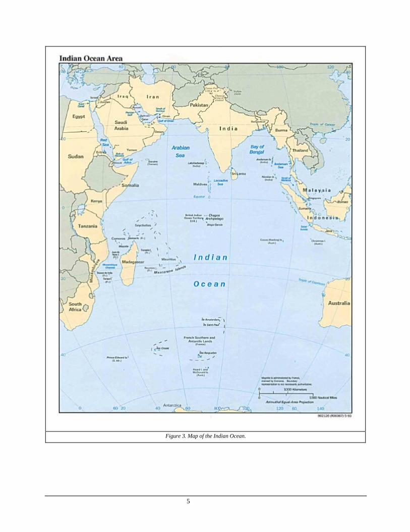
FIGURE 3. MAP OF THE INDIAN O CEAN. ................................................................................................. 5

FIGURE 4. PATTERNS OF SURFACE CURRENTS IN THE I NDIAN OCEAN BY MONSOON SEASON................... 6

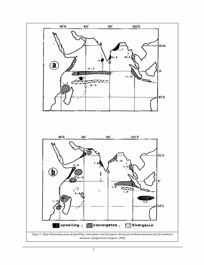
FIGURE 5. MAPS ILLUSTRATING AREAS OF UPWELLING, CONVERGENCE AND DIVERGENCE ..................... 6

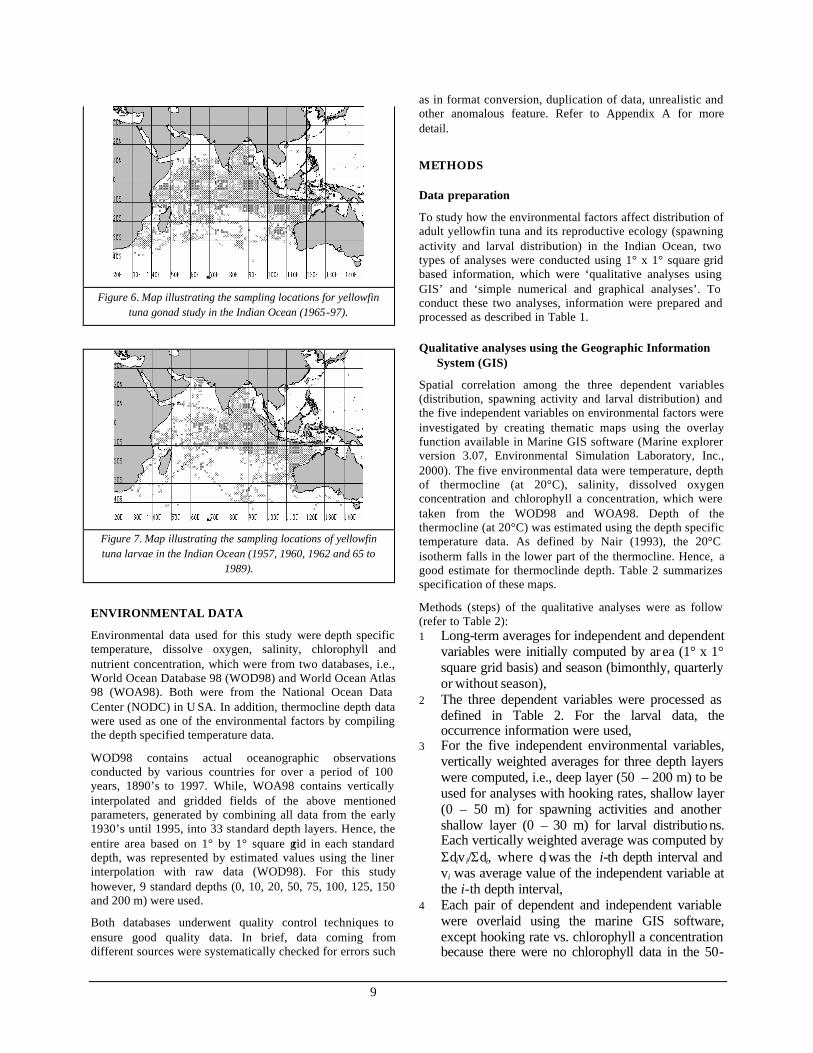
FIGURE 6. MAP ILLUSTRATING THE SAMPLING LOCATIONS FOR YELLOWFIN TUNA GONAD STUDY IN THE INDIAN O CEAN (1965-

97)................................. ................................ ................................ ................................ ....... 9

FIGURE 7. MAP ILLUSTRATING THE SAMPLING LOCATIONS OF YELLOWFIN TUNA LARVAE IN THE INDIAN OCEAN (1957, 1960,

1962 AND 65 TO 1989). ......................................................................................................... 9

FIGURE 8. EXAMPLE ILLUSTRATING APPROXIMATION OF OPTIMUM RANGE BASED ON RELATIONSHIP BETWEEN THE DEPENDENT

AND INDEPENDENT VARIABLES................................. ................................ ........................... 13

FIGURE 9 MAP ILLUSTRATING THE BIMONTHLY SAMPLING COVERAGE FOR YELLOWFI N TUNA GONADOSOMATIC STUDIES.

................................ ................................ ................................ ................................ ........... 20

FIGURE 10. MAP ILLUSTRATING THE BIMONTHLY SAMPLING COVERAGE FOR YELLOWFI N TUNA LARVAL SURVEY. 28

FIGURE 11. GRAPHS SHOWING THE RE LATIONSHIP BETWEEN H OOKING RATES AND ENVIRONMENTAL PARAMETERS IN THE 50-

200M DEPTH RANGE. ................................ ................................ ................................ ........... 36

FIGURE 12. GRAPHS SHOWING THE RE LATIONSHIP BETWEEN T HE COMPOSITION WHERE ≥41% ARE SEXUALLY MATURE

YELLOWFIN TUNA (YFT) AND ENVIRONMENTAL P ARAMETER IN THE 0-50M DEPTH RANGE. 38

FIGURE 13. GRAPHS SHOWING THE RELATIONSHIP BETWEEN LARVAL DENSITY AND ENVIRONMENTAL PARAMET ERS IN THE 0-

30M DEPTH RANGE . ............................................................................................................. 39

FIGURE 14. OPTIMUM SPECTRA OF VA RIOUS OCEANOGRAPHIC CONDITIONS THAT PRODUCE FAVORABLE HOOKING RATES (HR),

SPAWNING ACTIVITIES AND LARVAE DISTRIBUTION . ............................................................ 41

FIGURE 15. HYPOTHETICAL ILLUSTRA TION TO SHOW THE PRESENCE OF YELLOWFIN TUNA IN RELATION TO I SOBATHYTHERM OF

20°C (SOLID LINE). ............................................................................................................... 1

cccxlv

List of GIS Maps

Map 1a. (a) Map illustrating the overall distribution of yellowfin tuna with highest hooking rate (in X mark) overlaid on temperature (°C) profile at 50 m – 200 m deep in the Indian Ocean.Error! Bookmark not defined.

(b) Map illustrating the bimonthly distribution of yellowfin tuna with highest hooking rate (in X mark) overlaid on temperature (°C) profile at 50 m – 200 m deep in the Indian Ocean..............................14

Map 2 (a) Map showing the overall distribution of yellowfin tuna with highest hooking rate (in X mark) overlaid on salinity (psu) profile 50 m- 200 m deep in the Indian Ocean...............................................16

(b) Map illustrating bimonthly distribution of yellowfin tuna with highest hooking rate (in X mark) overlaid on salinity (psu) profile 50 m- 200 m deep in the Indian Ocean...............................................16

Map 3 (a) Map illustrating the overall distribution of yellowfin tuna with highest hooking rate (in X mark) overlaid on dissolved oxygen concentration (ml/L) profile at 50 m – 200 m deep in the Indian Ocean. Error! Bookmark not defined.

(b) Map illustrating the bimonthly distribution of yellowfin tuna with highest hooking rate (in X mark) overlaid on dissolved oxygen concentration (ml/L) profile at 50 m – 200 m deep in the Indian Ocean. 17

Map 4 (a) Map illustrating the overall distribution of yellowfin tuna with highest hooking rate (in X mark) overlaid on the isobath (m) of 20°C profile in the Indian Ocean. ...........................................................18

(b) Map illustrating the bimonthly distribution of yellowfin tuna with highest hooking rate (in X mark) overlaid on the isobath (m) of 20°C profile in the Indian Ocean. ................................ ......................19

Map 5 (a) Map illustrating the overall distribution of mature yellowfin tuna (in X mark) with more than 40% have GI ≥ 2.0 overlaid on the temperature ( °C) profile at 0 m –50 m deep in the Indian Ocean. ..............21

(b) Map illustrating the bimonthly distribution of mature yellowfin tuna (in X mark) with more than 40% have GI ≥ 2.0 overlaid on the temperature (°C) profile at 0 m –50 m deep in the Indian Ocean. ........22

Map 6 (a) Map showing the overall distribution of mature yellowfin tuna (in x mark) with more than 40% have GI ≥ 2.0 overlaid on salinity (psu) profile at 30 m – 50 m deep in the Indian Ocean........................22

(b) Map showing the bimonthly distribution of mature yellowfin tuna (in X mark) with more than 40% have GI ≥ 2.0 overlaid on the salinity (psu) profile at 30 m – 50 m deep in the Indian Ocean. ........23

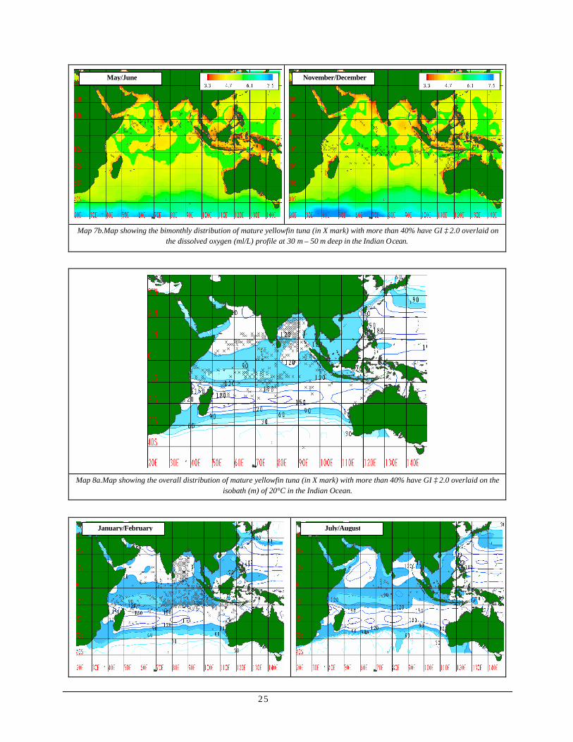
Map 7 (a) Map showing the overall distribution of mature yellowfin tuna (in X mark) with more than 40% have GI ≥ 2.0 overlaid on the dissolved oxygen (ml/L) profile at 30 m – 50 m deep in the Indian Ocean. 24

(b) Map showing the bimonthly distribution of mature yellowfin tuna (in X mark) with more than 40% have GI ≥ 2.0 overlaid on the dissolved oxygen (ml/L) profile at 30 m – 50 m deep in the Indian Ocean. 25

Map 8 (a) Map showing the overall distribution of mature yellowfin tuna (in X mark) with more than 40% have GI ≥ 2.0 overlaid on the isobath (m) of 20°C in the Indian Ocean.Error! Bookmark not defined.

(b) Map showing the bimonthly distribution of mature yellowfin tuna (in X mark) with more than 40% have GI ≥ 2.0 overlaid on the isobath (m) of 20°C depths in the Indian Ocean. ...............................26

Map 9 (a) Map showing the overall distribution of sexually mature yellowfin tuna (in X mark) with more than 40% have GI ≥ 2.0 overlaid on chlorophyll a (µg/L) concentration at 0 m deep in the Indian Ocean. Error! Bookmark not defined.

(b). Map showing the quarterly distribution of sexually mature yellowfin tuna (in X mark) with more than 40% have GI ≥ 2.0 overlaid on chlorophyll a (µg/L) concentration at 0 m deep in the Indian Ocean. 27

Map 10 (a) Map showing the overall occurrence of yellowfin tuna larvae overlaid on the temperature (°C) profile at 0 m – 30 m deep in the Indian Ocean. .........................................................................................29

(b) Map showing the bimonthly occurrence of yellowfin tuna larvae (in X mark) overlaid on the temperature (°C) profile at 0 m – 30 m deep in the Indian Ocean. ..........................................................30

Map 11 (a) Map showing the overall occurrence of yellowfin tuna larvae (in X mark) overlaid on the salinity (psu) profile at 0 m – 30 m deep in the Indian Ocean. ..................................................................30

(b) Map showing the bimonthly occurrence of yellowfin tuna larvae (in X mark) overlaid on the salinity (psu) profile at 0 m – 30 m deep in the Indian Ocean. ..................................................................31

Map 12 (a) Map showing the overall occurrence of yellowfin tuna larvae (in X mark) overlaid on the dissolve oxygen (mg/L) profile at 0 m- 30 m deep in the Indian Ocean.........................................................32

(b) Map showing the bimonthly occurrence of yellowfin tuna larvae (in X mark) overlaid on the dissolve oxygen (mg/L) profile at 0 m- 30 m deep in the Indian Ocean.........................................................33

cccxlvi

Map 13 (a) Map showing the overall occurrence of yellowfin tuna larvae (in X mark) overlaid on the isobath (m) of 20°C in the Indian Ocean...............................................................................................................33

(b) Map showing the bimonthly occurrence of yellowfin tuna larvae (in X mark) overlaid on the isobath (m) of 20°C in the Indian Ocean. ....................................................................................................34

Map 14 (a) Map showing the overall occurrence of yellowfin tuna larvae (in X mark) overlaid on chlorophyll a (µg/L) concentration at 0 m depth in the Indian Ocean...................................................................35

(b) Map showing the quarterly occurrence of yellowfin tuna larvae (in X mark) overlaid on chlorophyll a (µg/L) concentration at 0 m depth in the Indian Ocean...................................................................35

INTRODUCTION

The influence of the environment plays an important role, not only on its existence, but also on distribution, density and mortality of marine organisms as well. It predetermines the preferential habitat of different species whereby physiological adaptation is not subject to exceed its limits and tolerance. Though physical properties are not the only determinant, a good knowledge on this provides basis for understanding indirect effects on distribution such as availability of food.

Fisheries scientists are now considering ecological factors affecting major fisheries resources, indicative of their vulnerability to exploitation. For yellowfin tuna (Thunnus albacares), considerable work has been done to study their relationship with their habitat ranging from laboratory experiments to remote sensing or to real-time surveys. However, most of it is focused on distribution of catchable size and less attention at other life stages. Moreover, if not site specific, it is limited to smaller coverage area.

To date, only sea surface temperature data are mostly used to analyze the influence of environmental factors on yellowfin tuna distribution on a large-scale basis. Hence, it is necessary to study depth-specific environmental data, which corresponds to the depth range in different life stage (adult, spawners, larvae) of these species. Fortunately, the National Oceanic and Atmosp heric Administration through National Oceanographic Data Center (NODC) provides such depths specific oceanographic data in a long term period nearly for 100 years.

This paper is an attempt to describe environmental influences on the distribution of yellowfin tuna on an oceanic scale. Specifically, it will describe the influence of temperature, salinity, dissolved oxygen, thermocline depth, chlorophyll a and nutrients, on the distribution of adult, spawning activity and larvae of yellowfin tuna in the Indian Ocean. Further, it will attempt to predict optimal range of environmental parameters studied.

Limitation of the study includes none application of statistical tests to determine significance of influence of each environmental parameter. Also, few assumptions need to be considered for interpretation.

REVIEW

Biology and ecology

(1) Taxonomic description (Bonnaterre, 1788) Systematics

Class: Actinopterygii

Order: Perciformes

Family: Scombridae

Genus: Thunnus

Species: albacares

(2) Morphological Characteristics

Yellowfin tuna, Thunnus albacares (Bonnaterre, 1788), belongs to the family Scombridae. These fishes have elongated spindle-shaped (fusiform) bodies covered with small scales, having two separated dorsal fins, a deeply forked caudal fin and the presence of finlets behind the dorsal and anal fins. The second dorsal fin and anal fin are exceptionally long, and in some species may reach well over 20% of the fork length. The pectoral fin is moderately long, usually reaching beyond the second dorsal fin origin but not beyond the end of its base. Two small and one large keels are present in each side of the caudal peduncle. The color is black metallic, dark blue changing through yellow to silver on the belly. The dorsal and anal fins and finlets are bright yellow. The ventral side frequently has about 20 broken, almost vertical striation curved towards the rear (Figure 1).

Figure 1. Illustration of a yellowfin tuna (Thunnus albacares)

(3) Growth

Age and growth of yellowfin tuna have been studied through hardpart analysis (i.e. otolith, scales), weight and length frequency analysis by several authors (Stequert, 1989; Suzuki, 1994). Stequert (1989) cited that yellowfin tunas ages 1, 2, 3, 4 and 5 years have corresponding fork lengths 54 cm, 92 cm, 120 cm, 140 cm and 154 cm. Moreover, juveniles of 45-75 cm in fork length generally have the growth rate of 3 cm per month. In the Indian Ocean, a similar study showed that yellowfin tuna at 57-76 cm in fork length have the growth rate of 3 cm per month while 4.3 cm/mo at 88-101 cm. A review on the growth of yellowfin tuna revealed that the growth rate generally ranges from 2.7 to 3 cm/month at the size ranging from 30 cm to 100 cm (Ardill, 1993).

(4) Spawning and mode of reproduction

Yellowfin tunas attain sexual maturity at lengths ranging from 75.9 cm to 134.5 cm in fork length and age at first maturity is estimated to be 1.8 years (Froese, 1999).

Suzuki (1994) cited that the size of yellowfin tunas at first spawning (maturation) in the western and central Pacific has been studied through gonadosomatic indices (GSI), external features of the ovaries and microscopic examination of egg diameters. Results from one of the studies revealed that maturation ranges from 53 cm for males and 57 cm for females in Philippine waters while 70 -80 cm for females in the central Pacific. Another study also covering the area of western and central Pacific, revealed that maturation of females is attained at 80-110 cm in length.

2

Histological examination of ovaries revealed that the smallest female with mature ovaries in eastern tropical Pacific measured 84 cm in length. Studies from other authors, without histological examination, showed that the size at fifty percent maturity ranged from 110 cm to 120 cm in the western and central Pacific. Suzuki (1994) further cited that there were indications that yellowfin tunas caught by surface fisheries tended to be more mature than those taken by the longline fishery due to possible movement of mature individuals to the sur face layer. But, he stressed that there is a necessity for a detailed histological study on maturity covering both surface and longline data.

Stequert (1989), on the other hand, cited that an examination of yellowfin ovaries caught by longline fisheries in the Indian Ocean revealed that fifty percent of the fish observed reached first sexual maturity when measuring 120 cm to 140 cm and rarely at 80 cm in length. GSI levels of females in advanced ovarian development, range from 1.5 to 2.5. Plotting the distribution of mature females with GSI levels greater than 2, indicated spawning season and areas.

Yellowfin tunas have an external mode of fertilization (Froese, 1999). Eggs and sperm are released into the water column for fertilization. No parental care is given to the eggs or the young after spawning.

Yellowfin tunas spawn throughout the year in tropical and equatorial waters of three major oceans. At higher latitudes, spawning is seasonal, with peaks in summer. While at lower latitudes, it may continue throughout the year. There are also site specific seasonal peaks. In the western tropical Pacific, peak potentials are from December to January while April to May in the central tropical Pacific. Suzuki (1994) cited two authors whose studies revealed that there are two spawning peaks in the Philippines, a major peak in March to May and a lesser peak in October to December. Based on similarities between calculated birth date and other studies on gonad index, Stequert et al (1993) revealed that yellowfin tunas reproduce all year round with a peak between November and March in the Indian Ocean. In the previous study, Stequert (1989) specifically revealed that spawning intensifies from January to March in the central Indian Ocean as well as west off Sumatra and Seychelles. In the vicinity of Sri Lanka, it peaks from April to June, while it is October to December north off Australia and north of Madagscar.

Yellowfin tunas are multiple spawners and spawn every few days over the spawning period (Froese, 1999; Suzuki, 1994). In Suzuki’s review, yellowfin tunas in western Pacific spawned every 1.7 day while an interval of 1.3 days was observed in the eastern Pacific. Further, he cited that spawning occurs at 2000 to 2400 hours. He mentioned that some authors believe that spawning occurs during new moon and further suggested that it may be affected by the monsoon season, specifically in Philippine waters. Further, yellowfin tunas are multi-batch spawners (Timochina and Romanov 1991). They spawn 6–7 batches of eggs during spawning period in the western Indian Ocean. Sexual activity occurs during the months of November to February, while lasted inactivity from June to September.

(5) Larval stage

Larval stage in yellowfin tunas begins after hatching 1.34 to 1.85 days of egg development (Froese, 1999). The larvae live in the open ocean for a duration of 25 days. The optimum temperature is approximately 26.5°C. Suzuki (1994) further stated that the water temperature where the larvae are distributed ranges from 18.7°C to 31.9°C an d no larvae were found outside of that range. He also cited that there are two critical periods for larval mortality, 4 to 5 days and 11 days after hatching. The latter is associated with the change of prey from crustaceans to fish larvae. Kaji (1999), on the other hand, found that survival of tuna larvae was density dependent, observing a higher survival rate at high density and inversely for low density.

Suzuki (1994) cited from another source that yellowfin tuna larvae are more abundant at the surface first 50 m depth than in underlying subsurface water. He also cited that these larvae are more abundant during the night than during the day. Though he also mentioned that some believed that no diurnal differences occur, other studies indicate that larvae migrate to the surface during daytime.

(6) Feeding

Yellowfin tunas are a highly predatory species. Froese (1999) indicated that it has a trophic level ranging from 3.5 to 4.9 and feeds 11.6 times its body weight per year. They feed on a wide variety of prey species mainly nektons. Studies conducted using stomach content analysis revealed that yellowfin tunas prey on crustacean, cephalopods and finfishes (Froese 1999; Stequert, 1989). Suzuki (1994) cited that yellowfin tunas feed mostly during daytime and prey species composition varies with association with fish aggregating device (FAD). Some studies described that yellowfin tunas diet composition changes from one season to another while others indicated that there are no significant consumption rates between male and female. However, there is a high amount of juvenile yellowfin tunas being cannibalized.

In the western Indian Ocean, Roger (1993) conducted a study on the feeding behavior of surface tunas, in general, through stomach content analysis. His study also suggests that these tunas feed during the day foraging mainly on epipelagic prey fishes at prey-predator size ratio approximately 1:30. His study further suggests that tuna abundance is linked to plankton density due to intermediate characteristic of plankton feeding prey-fishes. Results also described that yellowfin tunas form small schools and feed on a wide variety of prey-fishes in poor areas. They just feed on what they meet in search for richer areas. Yellowfin tunas form large schools in rich areas, where they feed on large concentrations of a single type of prey-fish such as anchovies.

(7) Physiological adaptations

Yellowfin, as well as other tunas, continuously swim not only in search of prey but also to ventilate their gills and to maintain hydrostatic equilibrium. The intensity of swimming

3

activity consequently influences their oxygen demand. However, Stequert (1989) mentioned that the presence of a swim bladder among yellowfin tuna (which is not present in some genera) helps to regulate buoyancy and consequently ease the intensity of swimming activity, enabling them to reduce speed as well as oxygen intake.

Tuna’s unique aerobic locomotor (red) muscle, which power sustained swimming, has supporting vasculature that forms counter current heat exchangers. It conserves metabolic heat and acts as thermoregulation system. Stequert (1989) cited that juvenile tunas have to swim within narrower thermal boundaries due to underdeveloped thermoregulation system. Older individuals can penetrate deeper and colder waters.

Several laboratory experiments were conducted to examine yellowfin tuna’s physiological response to changes in temperature (Altringham, 1997), oxygen concentration and exercise (Korsmeyer, 1997). Field experiments through ultrasonic tagging were also conducted to ascertain ecophysiological preference of yellowfin tuna (Marsac, 1998; Brill, 1999; Block, 1997).

(8) Distribution

Horizontal distribution

There are numerous influences on the horizontal distribution of tunas in general. Hunter (1986) cited that aggregation of yellowfin tunas near the surface along oceanic provinces and other oceanic fronts are attributed to the abundance of food resources. He stressed that prediction of food abundance may depend on identification of the appropriate lag between the onset of a productivity event and tuna catches. Added to that, oceanographic processes such as divergent zones determine food production and distribution. He identified that tunas are rarely found in these zones. Instead, they frequented zones of convergence where laterally dispersed food are collected. The same is true for eddy motions which can create divergence or convergence depending on the direction of the flow and coriolis force. Moreover, he also mentioned that yellowfin tunas tend to remain in clear oceanic waters and avoid low visibility or turbid coastal waters.

Stequert (1989) further conveyed the implication of potential of tertiary productivity enhanced by primary and secondary productivity along upwelling regions. However, the concept remains theoretical due to the complexities in the maturation process of phytoplankton enriched water masses and effects of multiple predation. Added to that, he also pointed out that high metabolic activity of tunas force them to constantly engage in the search for suitable areas to ensure their survival. Hence, tunas, in general, are concentrated according to a hydrological route or optimum environment rather than areas of high primary productive. He also identified potential tuna concentration in the Indian Ocean based on physiological compatibility of tunas to zones of optimal temperature and dissolved oxygen levels.

Marsac (1998) discussed potential dwelling time of tunas to FAD. He mentioned that yellowfin tunas move closer to the

FAD during t he day than at night. He attributed his observations to an attraction effect exerted by the vertical anchor line. He further said that device aggregates other small prey species, which act as stimulus to retain the predator within the vicinity.

Suzuki (1994) cited seasonal movement to higher latitude during warm season and to lower latitude along major currents in the Pacific. The fact that several tagged yellowfin tunas in the equatorial Pacific were recovered in the temperate waters of Japan indicates pot ential long-distance migration. He also cited that distribution can be affected by oceanographic factors such as surface water temperature.

Vertical distribution

Generally, yellowfin tunas are found above or within the thermocline with an occasional dive beneath the thermocline (Cayre, 1993; Block, 1997). Carey et al (1993) pointed out that gradients of temperature and dissolved oxygen have greater effect on the vertical movement of yellowfin tuna. In western Indian Ocean, oxygen levels ranging from 3.6 to 4.2 ml O2 per liter can be considered threshold values that could affect the general activity of the species. Block (1997), on the other hand, found temperature to be the limiting factor rather than oxygen levels near the Hawaiian Islands. John (1995) in his study, further elaborated the relationship between thermal processes and catch per unit effort (CPUE) along the exclusive economic zone of India. He stated that CPUE based on longline fishing, is positively associated with mixed-layer depth and thermal gradients while negatively related to isotherm depth, column thickness, thermocline depth and thermocline thickness. He described that the preferred temperature zone is compressed when the vertical thermal gradient is high, resulting to a higher density of fish per unit volume.

Schooling is a common behavior of fishes to aggregate themselves purposely as a protection measure. Stequert (1989) described some patterns of deep-sea schooling detected by echo sounder in the Indian Ocean. Schools mostly detected below flotsam appear in one compact form and are comprised of mixed species of adult skipjack, juvenile yellowfin and bigeye tunas. Schools may also have two forms or groups, one on top of the other. The top part is usually compact in form, comprised of smaller individuals, while the underlying are elongated and composed of larger individuals. Schools displaying a single but extremely elongated form, are composed of larger individuals. The depth distribution of the three patterns of schooling ranges from 10 m to 70 m, 15 m to 130 m and 30 m to 130 m, respectively.

FISHERIES

(1) General

Tuna and tuna-like species are mostly caught with purse-seine, longline and pole-and-line in three major oceans. The purse seine and pole-and-line methods are used to catch fish found close to the surface (e.g. skipjack and relatively small

4

individuals of yellowfin, albacore and northern and southern bluefin tuna). The longline method, on the other hand, targets fish found at greater depths, e.g. large individuals of northern and southern bluefin tuna, bigeye tuna, yellowfin and albacore. Most purse seine and pole-and-line catches are canned, while longline catches, with the exception of those of albacore, are mainly sold on the sashimi market to be consumed raw, essentially in Japan. Other gears are troll lines, hand lines, driftnets, traps and harpoons. Natural or artificial FAD are often used in conjunction with purse seining or hand lining.

The global catch of yellowfin tuna is continuously increasing from 0.1 million metric tons in the 1950’s to 1.1 million metric tons in 1997. Twenty seven percent of the global yellowfin catch comes from the Indian Ocean, amounting to 305 thousand metric tons which the majority is landed by purse seine (41%) followed by longline (34%) and gillnet (11%).

(2) Longline fisheries

Longline fishing is a method of catching fish using baited hooks in a series of branch lines attached to a single mainline. Bottom and surface setting are two modes of operating the gear. For the former, the mainline is anchored at the seabed. The main target of this setting are demersal fishes and hence, it will not be dealt in this paper. In surface longlining on the other hand, the mainline is suspended in the water column using a floating device. It mainly targets adult tuna, swordfish and other large predatory fishes. The line is set as the boat moves forward. Once the line is fully extended, it is hauled in.

Japanese tuna longliners have two types of longlining practices (Koido, 1985; Mohri, 1998). The first is by the use regular gear structured longline. It is characterized by having eight or less branch lines or hooks per basket. While the second is the use of deep longline gear structure having nine or more hooks per basket (Figure 2).

Figure 2. Illustration on the two types of Japanese longline fishing gear commonly used. The left shows the regular longline, normally with hooks ≥ 8, while the right, for the deep longline, normally with

hooks ≥ 9 (adapted from Mohri, 1998).

MARINE EN VIRONMENT

The Indian Ocean is the smallest of the earth's three major oceans with total area of about 73.4 million km 2 (Figure 3). It is bounded on the west by the African continent, on the north by Asian continent, on the east by Australia and Indonesian Archipelago, and on the south by Antarctica. The ocean narrows toward the north, and is divided by the Indian peninsula into the Bay of Bengal on the east and the Arabian Sea on the west. The Arabian Sea sends two arms northward, the Persian Gulf and the R ed Sea. The average depth of the Indian Ocean is about 4,210 m (about 13,800 ft), or slightly greater than that of the Atlantic, and the deepest known point is about 7,725 m (about 25,344 ft), off the southern coast of the Indonesian island of Java. In general, the greatest depths are situated in the northeastern sector of the ocean, where about 129,500 km2 of the ocean floor lie at a depth of more than 5,486 m (18,000 ft).

The Indian Ocean contains numerous islands, the largest of which are Madagascar and Sri Lanka. Smaller islands include the Maldive atolls made by coral reefs and Mauritius. From Africa, the Indian Ocean receives the waters of the Limpopo and Zambezi Rivers, and from Asia those of the Irrawaddy, Brahmaputra, Ganges, Indus, and Shatt al Arab Rivers.

Environmental conditions in the Indian Ocean were best described by Stequert and Marsac (1989). In brief, the ocean is affected by two seasonal winds called monsoons, the northeast monsoon which prevails from December to March and the southwest monsoon which prevails from June to September. In between are inter -monsoon season which range from April to May and from October to November. The general current flow is shown in Figure 4. Figure 5 illustrates the upwelling, convergence and divergence ar eas.

5

Figure 3. Map of the Indian Ocean.

6

Figure 4. Patterns of surface currents in the Indian Ocean by monsoon season; (a) northeast monsoon and (b) southwest monsoon. (adapted from Nishida, 1991)

7

Figure 5. Maps illustrating areas of upwelling, convergence and divergence during (a) northeast monsoon and (b) southwest

monsoon. (adapted from Stequert, 1989)

8

PREVIOUS STUDIES

Majority of related studies focus mainly on environmental influences using mainly sea-surface temperature to yellowfin tuna distribution while spawning activities and larval ecology are dealt independently. There are no previous studies dealing with various depth-specific oceanographic parameters synthetically.

Dewar et al. (1994) conducted laboratory experiment to describe the reduction of potential limitations to distribution and the efficiency in exploiting cooler waters through physiological thermoregulation. However, their study was limited to physiological responses rather than distribution. Cayre et al. (1993), Block (1997) and Brill (1999) studied yellowfin tuna distribution related to environmental conditions through ultra-sonic tracking and CTD casts. Cayre (1993) conveyed that temperature gradients and dissolved oxygen explains the vertical distribution of young yellowfin tunas. Block (1997) on the other hand, revealed that yellowfin tuna with size ranging from approximately 4 kg to 110 kg have strong environmental preference whereby tracked specimen were consistently found above the thermocline in the surface mixed layer in waters near California, United States. Brill (1999) also relate temperature to be the limiting factor in his experiment near the Hawaiian Islands.

Kumari et al. (1993) and Nair et al. (1993) made use of fisheries data to study influences of environmental conditions on yellowfin tuna caught in the Indian waters. Kumari (1993) studied the distribution of tuna in general in response to sea surface temperature data from satellite imagery. He concluded that fishery optima lie between water temperature range of 27°C to 29°C. Nair (1993), on the other hand, studied the influence of temperature specifically on yellowfin tuna fishery through statistical analysis based from climatological data obtained from National Oceanographic Data Center. Mohri (2000), on the other hand, also made use of Japanese longline fisheries data in the Indian Ocean and relate it to temperature and dissolved oxygen concentration data obtained from their nat ional oceanographic data center.

Less attention is given on studies related to environmental influences on spawning activity. Shung (1973) revealed that yellowfin tuna’s sexual activity is not influenced by temperature since it remained high and low at temperature 26°C and above.

Likewise, studies on environmental influences on yellowfin tuna larval distribution are understudied. Boehlert (1994) studied larval distribution of tunas in general through ichthyoplankton surveys using multiple opening-closing net and environmental sensing system (MOCNESS) in Hawaiian waters. He discussed association of tuna larval distribution and physical characteristics of their habitat as defined by temperature. He also discussed the association of yellowfin tuna larvae and the presence of land.

In addition, no studies have conducted about the nutrients effects on different life stage of yellowfin tuna.

Information

Four types of information were used in this study, i.e., Japanese commercial tuna longline fisheries data, gonad (sexual maturity) data, larval data and environmental data. A detailed explanation of each of these information are given below.

Commercial tuna longline fisheries data.

The Japanese commercial tuna longline fisheries data were obtained from the database of the National Research Institute of Far Seas Fisheries (NRIFSF) of Japan. From this database, locations, operation months, catch (number) and effort (number of hooks) data from 1953 to 1997 in the Indian Ocean were extracted for this study. Only regular longline data were used and deep longline data were not used because deep longliners target bigeye tuna (Thunnus obesus), while the regular longliners target yellowfin tuna, hence their species compositions between these two gears were different. Therefore, only regular longline data were used to maintain homogeneous quality of the catch and effort data.

Gonad data

Gonad data were obtained from the survey data of the Japan Marine Fishery Resources Research Center (JAMARC) and also from the database of NRIFSF . The former data were collected from experimental longline fishing in the Indian Ocean conducted over the period of six years, 1981 to 1986. The latter data were collected from fisheries high school training vessel and prefecture fisheries experimental station vessel over the period of thirty-three years, 1965 to 1997. See Figure 6 for an overall sampling coverage.

Larval data

Larval data were from the NRIFSF database, including sampling date and time, locations, methods, and number of larvae sampled. Original data were collected by the research vessels belonging to the Fisheries Agency of Japan and other vessels (fishing high school training vessels and prefecture fisheries experimental station vessels) over the period of 28 years (1957, 1960, 1962 and 65 to 89). See Figure 7 for the sampling coverage.

All of the vessels used a conical larval net with identical mesh size of 1.7 mm at the anterior portion, two-third of the net and 0.5 mm at the posterior end. However, sampling conditions varied. The research vessels used a larger net of 2 m in diameter and 6m in length. Day and night tows were made horizontally at subsurface level of approximately 20-30 m deep. The high schools and training vessels, on the other hand, used a smaller net of 1.4 m in diameter and 4 m in length. Surface tows were done during the nighttime. Tows were generally made at an average speed of two knots. In the qualitative (GIS) analyses, information from both research and other vessels were used, while in the qualitative (numerical) analyses, information only from research vessels were used because of consistent method in data collection. Thus, they are high quality information.

9

Figure 6. Map illustrating the sampling locations for yellowfin tuna gonad study in the Indian Ocean (1965-97).

Figure 7. Map illustrating the sampling locations of yellowfin tuna larvae in the Indian Ocean (1957, 1960, 1962 and 65 to

1989).

ENVIRONMENTAL DATA

Environmental data used for this study were depth specific temperature, dissolve oxygen, salinity, chlorophyll and nutrient concentration, which were from two databases, i.e., World Ocean Database 98 (WOD98) and World Ocean Atlas 98 (WOA98). Both were from the National Ocean Data Center (NODC) in U SA. In addition, thermocline depth data were used as one of the environmental factors by compiling the depth specified temperature data.

WOD98 contains actual oceanographic observations conducted by various countries for over a period of 100 years, 1890’s to 1997. While, WOA98 contains vertically interpolated and gridded fields of the above mentioned parameters, generated by combining all data from the early 1930’s until 1995, into 33 standard depth layers. Hence, the entire area based on 1° by 1° square grid in each standard depth, was represented by estimated values using the liner interpolation with raw data (WOD98). For this study however, 9 standard depths (0, 10, 20, 50, 75, 100, 125, 150 and 200 m) were used.

Both databases underwent quality control techniques to ensure good quality data. In brief, data coming from different sources were systematically checked for errors such

as in format conversion, duplication of data, unrealistic and other anomalous feature. Refer to Appendix A for more detail.

METHODS

Data preparation

To study how the environmental factors affect distribution of adult yellowfin tuna and its reproductive ecology (spawning activity and larval distribution) in the Indian Ocean, two types of analyses were conducted using 1° x 1° square grid based information, which were ‘qualitative analyses using GIS’ and ‘simple numerical and graphical analyses’. To conduct these two analyses, information were prepared and processed as described in Table 1.

Qualitative analyses using the Geographic Information System (GIS)

Spatial correlation among the three dependent variables (distribution, spawning activity and larval distribution) and the five independent variables on environmental factors were investigated by creating thematic maps using the overlay function available in Marine GIS software (Marine explorer version 3.07, Environmental Simulation Laboratory, Inc., 2000). The five environmental data were temperature, depth of thermocline (at 20°C), salinity, dissolved oxygen concentration and chlorophyll a concentration, which were taken from the WOD98 and WOA98. Depth of the thermocline (at 20°C) was estimated using the depth specific temperature data. As defined by Nair (1993), the 20°C isotherm falls in the lower part of the thermocline. Hence, a good estimate for thermoclinde depth. Table 2 summarizes specification of these maps.

Methods (steps) of the qualitative analyses were as follow (refer to Table 2): 1 Long-term averages for independent and dependent

variables were initially computed by ar ea (1° x 1° square grid basis) and season (bimonthly, quarterly or without season),

2 The three dependent variables were processed as defined in Table 2. For the larval data, the occurrence information were used,

3 For the five independent environmental variables, vertically weighted averages for three depth layers were computed, i.e., deep layer (50 – 200 m) to be used for analyses with hooking rates, shallow layer (0 – 50 m) for spawning activities and another shallow layer (0 – 30 m) for larval distributions. Each vertically weighted average was computed by Σdiv i/Σdi, where di was the i-th depth interval and vi was average value of the independent variable at the i-th depth interval,

4 Each pair of dependent and independent variable were overlaid using the marine GIS software, except hooking rate vs. chlorophyll a concentration because there were no chlorophyll data in the 50-

10

200m depth range. Thus, 14 GIS maps (3 dependent x 5 independent - 1) were created,

5 For each pair of dependent and independent variables, two types of GIS maps were created, i.e.,

one for the overall average without season and the other for the seasonal maps (bi-monthly or quarterly).

Table 1. Summary of information and definitions of variables. Information and definition of variables

for the analyses

Types of variables

Description of

parameters

Name of variables

Depth range

(*) Qualitative analyses using GIS

Simple numerical and graphical analyses

Distribution

Hooking rates Mid-water (50-200m)

(Information) Japanese tuna longline database (NRIFSF) (Definition) number of fish/1000 hooks High hooking rates ≥ 13.4 (3rd quartile of hooking rates)

Spawning activities :

composition (%) of mature

YFT

Shallow (0-50m)

(Information) Larval data (JAMARC and NRIFSF) (Definition) (no. mature fish x 100) /(total no. of fish), where mature fish was defined by the gonad index (GI) > 2.0, GI=female gonad weight x 104 / L3

Larval distribution

(Information) Larval database (NRIFSF) (Definition) 1x1 area where at least one larvae found were mapped.

Dependent

Reproductive ecology

Larval density

Shallow (0-30m)

(Information) larval database, (NRIFSF) (Definition) Number of larvae per tow. Only research vessels data are used because of their accurate and consistent sampling methods

Temperature Salinity

Basic factors

Dissolve oxygen

Depth of thermocline

Thermocline depth

at 20oC

Three depth layers

(50-200m, 0-50m, 0-30m) Independent

(Environmental data)

Nutrients (primary

productivity)

Chlorophyll

Two shallow layers

(0-30m and 0-50m)

(Information) WOD98 & WOA98 (Definition) For the GIS mappings, variables were presented either by symbols or contours.

(Data) WOA98 (Definition ) Vertically weighted averages, for three depth layers were used to represent independent variables, which were computed by Σdivi/Σdi, where di

is the i-th depth interval and v i is average value of the independent variable at the i-th depth interval.

Three types of presentation techniques were used in representing parameters, which were ‘symbol’, ‘image’ and ‘contour’. ‘Symbol’ was used to present location and density of parameters. ‘Image’ was used for presenting matrix data (array data) such as remotely sensed images of satellite images. Though intervals can be manipulated, values were represented in raster form, occupying certain grids that corresponds to the coloration assigned. Contour maps, on t he

other hand, were produced from point data of actual observations and values. Isolines were then generated by kriging, a special interpolation technique (linear variogram) where estimates were computed based on known and existing values. In this study, these three presentation techniques were used to present each parameter effectively. Table 2 indicates how these presentation techniques were applied.

11

Table 2. Specification of the GIS thematic maps to investigate spatial correlation between 3 dependent and 5 independent variables.

Dependent

Variable

(DEP_V)

Hooking rates

(no. of YFT/1000 hooks)

Spawning activity

(%of mature YFT)

Larval distribution

(occurrence of YFT larvae)

Period (DEP_V) 45 years

(1953-97)

28 years

(1957, 60, 62, 65-89)

33 years

(1965-97)

Period (IND_V) Over 100 years (1890’s –1997) (more than 95% were from 1953-97)

Spatial scale

(pixel unit)

1x1 degree square grid area

Depth scale Deep (50-200m) Shallow (0-50m) Shallow (0-30m)

Presentation

In GIS maps

(DEP_V) symbol

(IND_V) image

(DEP_V) symbol

(IND_V) countour

(DEP_V) symbol

(IND_V) countour

Independent (environmental variables)

(IND_V)

Temperature

(oC)

Overall mean (Map 1a)

Bi-monthly mean (Map 1b)


Bi-monthly (Map 5b)



Salinity

(psu)



Overall (Map 6a)

Bi-monthly (Map 6b)



Oxygen

(ml/L)



Overall (Map 7a)

Bi-monthly (Map 7b)



Chlorophyll

(micro mol)

(not analyzed

because of no data)


Quarterly mean (Map 8b)(*)


Quarterly mean (Map 13b)(*)

Depth of thermocline

(m)(at 20oC)







(*) : Data only from surface (0m)

Numerical analyses

Simple numerical analyses were conducted to investigate quantitative relationships between the three dependent variables (hooking rates, spawning activities and larval distribution) and eight independent (environmental) variables by depth range. The eight environmental data were temperature, depth of thermocline (at 20°C), salinity, dissolved oxygen concentration, chlorophyll a concentration and nutrients (phosphate, silicate and nitrate), which were all taken from WOA98 (1° x 1° square grid basis interpolated data in nine standard depths i.e., 0, 10, 20, 30, 50, 75, 100, 150 and 200m). The depth of the thermocline data (at 20°C) was estimated using the depth specific temperature data.

The methods (steps) of the numerical analyses were as follow (refer to Table 3): 1 Long term averages of the independent and

dependent variables were initially computed by area (1° x 1° square grid basis), season (bimonthly or quarterly) and standard depth,

2 The three dependent variables were processed as defined in Table 1. For the larval data, the number of larvae per tow (sample) was used,

3 For the five independent environmental variables, vertically weighted averages for three depth layers

were computed, i.e., deep layer (50–200 m) to be used for analyses with hooking rates, shallow layer (0–50 m) for spawning activities and another shallow layer (0–30 m) for larval distributions. Each vertically weighted average was computed by ∑divi/∑di, where di was the i-th depth interval and vi was average value of the independent variable at the i-th depth interval,

4 The independent and the dependent variables were merged and matched by same time-area-depth layer unit. If there were missing values in some time-area-depth layer unit after the merge, they was not used,

5 Each independent variable was arranged in equal intervals sorting dependent variable in each respective interval,

6 Averages for each dependent variable were computed in each interval of the independent variables. This average values was referred to as ‘Observed’ values,

7 Further, an overall weighted average was computed for the three dependent variables and referred to as ‘Average’ values. This overall average was also the criterion or cut-off points in determining the optimum range of independent

12

variable that produce favorable effect on the dependent variables.

8 Then, both values were plotted on line graphs totaling to 23 graphs (see Table 3) that shows relationships between the dependent and independent variables,

9 Ranges of independent variables that produced more than the cut-off point values of the dependent variables were defined as the ‘optimum range’. Spectra of these ranges were created (see the illustration in Figure 8).

Table 3. Specifications of the graphs (plots) for the numerical analyses.

Dependent variables è Unit Hooking rates (*) (no. of fish/1000 hooks)

Spawning activities (%of mature YFT)

Larvae distribution (no. of larvae per tow)

Depth range Deep (50-200m) Shallow (0-50m) Shallow (0-30m)

Independen variables

Temperature (oC)

Depth of thermocline (20oC) (m)

Salinity (psu)

Dissolved Oxygen (ml/L)

Mo (Figure 9)

Chlorophyll (µM) NA

Mo (Figure 10) Mo (Figure 11)

Phosphate (µM)

Silicate (µM)

Nitrate (µM)

Q (Figure 9) Q (Figure 10) Q (Figure 11)

RESULTS

QUALITATIVE ANALYSES USING GIS

Hooking rates vs. Environmental factors

In order to delineate potential abundance of yellowfin tuna among the catches, only the high hooking rate was mapped against environmental factors. High hooking rate was defined by the extreme hooking rates with values greater than third quartile (13.4 fish/1000 hooks).

High hooking rates (>13.4 fish/1000hooks) vs. Temperature for the 50-200m depth range (Map 1)

Map 1a shows the overall occurrence of high hooking rates overlaid on temperature profile in the Indian Ocean. Density of hooking rates was localized a little south of the equator, inclined towards the western Indian Ocean and far reaching towards the northern portion of Mozambique Channel. Mass occurrence of high hooking rate was also observed along the Indian peninsula, surrounding waters of Sri Lanka and the Andaman Islands. Water temperature in these areas was approximately around 17.5°C. While high hooking rates were limited in the Arabian Sea and waters in between the 10oS and 30°S latitudes where water temperature was reaching warmer level. Dense high hooking rates occurring towards the western side of the basin, seemed to be associated with an observable stretch of much lower water temperature ranging from 17.5°C or below. found at 0o to 10oS and 50 oE to 80oE.

Map 1b shows the bimonthly distribution of high hooking rates overlaid on temperature profile in the Indian Ocean. The density of high hooking rates were likely to show an association with the profile of the water low temperature

found in the equatorial region. In January/February, the density of high hooking rates forms a semi-solid cluster within the range of the low water temperature area, 0-10 oS and 40-80 oE. In March/April, this cluster tended to loosen up as the low water temperature area elongated, spreading towards the eastern Indian Ocean. Also, occurrence of low water temperature draws in aggregation off the western coast of Sumatra, the Andaman Sea and northern part of Bay of Bengal. Apparent warming of the Arabian Sea seemed to limit the occurrence of high hooking rates sparsely distributed in the central portion.

In May/June, occurrence of high hooking rates was widely spread in the equatorial region stretching as far as the area of Bay of Bengal. Though occurrence was not observe in the warmer waters in the Arabian Sea at this period, a cluster seemed to appear in the warmer water of the eastern Indian coast. Density of occurrence reduced by July/August even though it remained scattered in the equatorial region.

In September/October, the low temperature area in the equatorial region further shrank back towards the eastern coast of Africa while density of high hooking rate diminished and scattered in the equatorial region. Also in this period, the optimum lower temperature region also seemed to shrink back with some low water temperature occurrence along west coast off Sumatra and the area within the vicinity of Sri Lanka. A noticeable difference in temperature profile was visible. A series of colder waters enclosed and separated a fairly cold water mass from warmer ambient waters in the western Indian Ocean, which was considered to be caused by the southwest monsoon. In November/ December, the density began to rebuild off the east African coast occupying a much compact region of low water temperature.

13

Figure 8. Example illustrating approximation of optimum range based on relationship between the dependent and independent

variables.

Map 1a. Map showing the overall distribution of yellowfin tuna with highest hooking rate (in X mark) overlaid

on temperature (°C) profile at 50–200 m deep in the Indian Ocean.

1 7 . 0 1 7 . 5 1 8 . 0 1 8 . 5 1 9 . 0 1 9 . 5 2 0 . 0 20.5 2 1 . 0 2 1 . 5 2 2 . 0 2 2 . 5 2 3 . 0 23.5 24.0 2 4 . 5 2 5 . 0 2 5 . 5 2 6 . 0 2 6 . 5 2 7 . 0 2 7 . 5 2 8 . 0 2 8 . 5 2 9 . 0 2 9 . 5 3 0 . 0

H R

( 5 0 - 2 0 0 m )

Cut-off points

14

Map 1b. Map showing the bimonthly distribution of yellowfin tuna with highest hooking rate (in X mark) overlaid on temperature (°C) profile at 50–200 m deep in the Indian Ocean.

November/December May/June

September/October March/April

July/August January/February

15

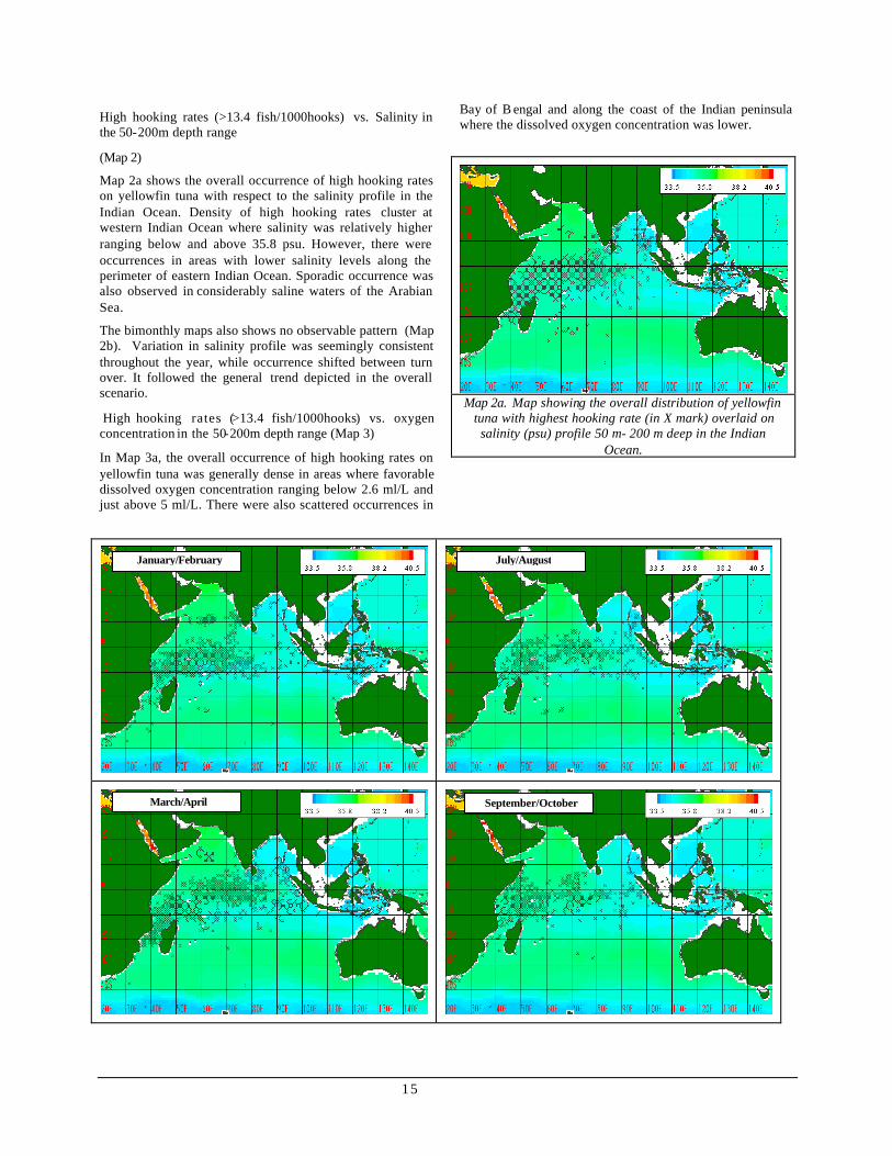
High hooking rates (>13.4 fish/1000hooks) vs. Salinity in the 50-200m depth range

(Map 2)

Map 2a shows the overall occurrence of high hooking rates on yellowfin tuna with respect to the salinity profile in the Indian Ocean. Density of high hooking rates cluster at western Indian Ocean where salinity was relatively higher ranging below and above 35.8 psu. However, there were occurrences in areas with lower salinity levels along the perimeter of eastern Indian Ocean. Sporadic occurrence was also observed in considerably saline waters of the Arabian Sea.

The bimonthly maps also shows no observable pattern (Map 2b). Variation in salinity profile was seemingly consistent throughout the year, while occurrence shifted between turn over. It followed the general trend depicted in the overall scenario.

High hooking rates (>13.4 fish/1000hooks) vs. oxygen concentration in the 50-200m depth range (Map 3)

In Map 3a, the overall occurrence of high hooking rates on yellowfin tuna was generally dense in areas where favorable dissolved oxygen concentration ranging below 2.6 ml/L and just above 5 ml/L. There were also scattered occurrences in

Bay of B engal and along the coast of the Indian peninsula where the dissolved oxygen concentration was lower.

Map 2a. Map showing the overall distribution of yellowfin

tuna with highest hooking rate (in X mark) overlaid on salinity (psu) profile 50 m- 200 m deep in the Indian

Ocean.



16

Map 2b. Map showing the bimonthly distribution of yellowfin tuna with highest hooking rate (in X mark) overlaid on salinity (psu) profile 50 m- 200 m deep in the Indian Ocean.

In bimonthly occurrence of high hooking rates overlaid on oxygen concentration (Map 3b), dense aggregation apparently followed the varying patterns of dissolved oxygen concentration. In January/February, a dense cluster was situated within the bounds of favorable range, around 2.6 ml/L to 5.0 ml/L dissolved oxygen concentration in the equatorial region, although there was some sporadic occurrences at Bay of B engal where there was lower level of dissolved oxygen concentration. In March/April, favorably oxygenated waters seem encroaching inward Arabian Sea while a lower dissolved oxygen concentration level dominated in the Bay of Bengal. In coherence, diminishing occurrence could be observed inner of Bay of Bengal at this period. Unlikely for May/June, the spread of favorable dissolved oxygen concentration level in the Arabian Sea did not show a similar density of aggregation. Moreover, dense aggregation appeared in the Bay of Bengal where lower

oxygen level prevailed, although there were spots of higher dissolved oxygen concentration on either side of the Bay. In July/August, evident non-occurrence was shown in areas of low dissolved oxygen level that prevails in the northern Indian Ocean. Same pattern could be found during September/October. In November/December, the dense aggregation was further pushed towards the equator as low dissolved oxygen level dominated the Arabian Sea and Bay of Bengal, though there were sparse occurrences within the Bay.

High hooking rates (>13.4 fish/1000hooks) vs. Thermocline depth (Map 4)

The overall occurrence of high hooking rates on yellowfin tuna with respect to the depth of thermocline (Map 4a) was widely distributed at different depths, though the bulk was situated within depths of 120 m and shallower along the

equator.

Map 4b shows the bimonthly occurrence of high hooking rates on yellowfin tuna with respect to the depth of thermocline. The spread of the high hooking rates vaguely followed the course of thermocline depth throughout each month. In January/February, preferred thermocline depth was generally situated along and southwest of the equatorial region with some occurrence in the middle of Arabian Sea. Density of high hooking rates also shows the same pattern. In March/April and May/June, shallow thermocline depth break down at the western side and seemed to shift its spread at the eastern side of the ocean just as the high hooking rates seemed to spread and becoming dens er at the eastern Indian Ocean. However, in the 2nd half of the year, the density of high hooking rates remaining in the equatorial region did not seem to be affected even though the range of the shallower thermocline depth extended northwards.


Map 3a. Map showing the overall distribution of yellowfin tuna with highest hooking rate (in X mark) overlaid on dissolved oxygen

concentration (ml/L) profile at 50–200 m deep in the Indian Ocean.

17

Map 3b. Map showing the bimonthly distribution of yellowfin tuna with highest hooking rate (in X mark) overlaid on dissolved oxygen

concentration (ml/L) profile at 50–200 m deep in the Indian Ocean.




18

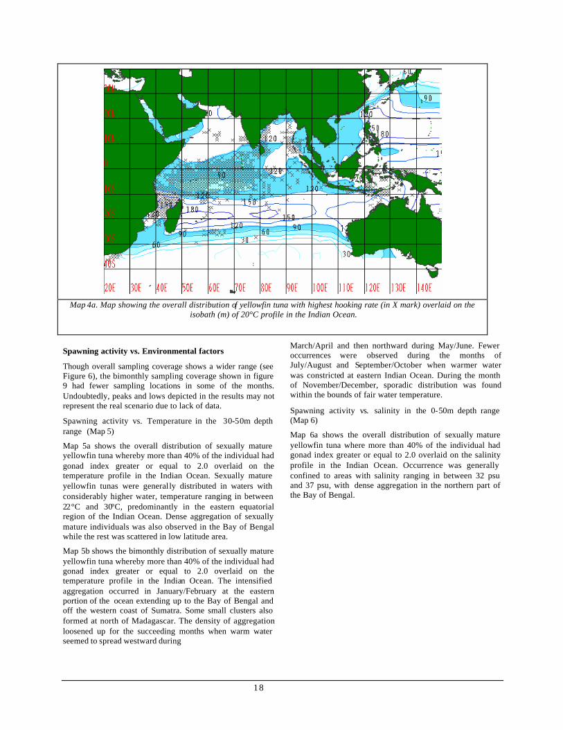
Map 4a. Map showing the overall distribution of yellowfin tuna with highest hooking rate (in X mark) overlaid on the

isobath (m) of 20°C profile in the Indian Ocean.

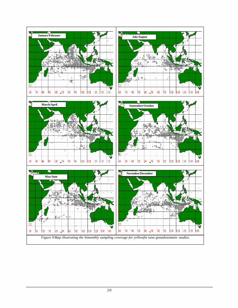
Spawning activity vs. Environmental factors

Though overall sampling coverage shows a wider range (see Figure 6), the bimonthly sampling coverage shown in figure 9 had fewer sampling locations in some of the months. Undoubtedly, peaks and lows depicted in the results may not represent the real scenario due to lack of data.

Spawning activity vs. Temperature in the 30-50m depth range (Map 5)

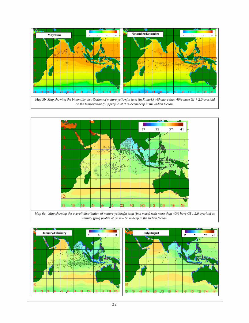
Map 5a shows the overall distribution of sexually mature yellowfin tuna whereby more than 40% of the individual had gonad index greater or equal to 2.0 overlaid on the temperature profile in the Indian Ocean. Sexually mature yellowfin tunas were generally distributed in waters with considerably higher water, temperature ranging in between 22°C and 30°C, predominantly in the eastern equatorial region of the Indian Ocean. Dense aggregation of sexually mature individuals was also observed in the Bay of Bengal while the rest was scattered in low latitude area.

Map 5b shows the bimonthly distribution of sexually mature yellowfin tuna whereby more than 40% of the individual had gonad index greater or equal to 2.0 overlaid on the temperature profile in the Indian Ocean. The intensified aggregation occurred in January/February at the eastern portion of the ocean extending up to the Bay of Bengal and off the western coast of Sumatra. Some small clusters also formed at north of Madagascar. The density of aggregation loosened up for the succeeding months when warm water seemed to spread westward during

March/April and then northward during May/June. Fewer occurrences were observed during the months of July/August and September/October when warmer water was constricted at eastern Indian Ocean. During the month of November/December, sporadic distribution was found within the bounds of fair water temperature.

Spawning activity vs. salinity in the 0-50m depth range (Map 6)

Map 6a shows the overall distribution of sexually mature yellowfin tuna where more than 40% of the individual had gonad index greater or equal to 2.0 overlaid on the salinity profile in the Indian Ocean. Occurrence was generally confined to areas with salinity ranging in between 32 psu and 37 psu, with dense aggregation in the northern part of the Bay of Bengal.

19

Map 4b. Map showing the bimonthly distribution of yellowfin tuna with highest hooking rate (in X mark) overlaid on

the isobath (m) of 20°C profile in the Indian Ocean.




20

Figure 9 Map illustrating the bimonthly sampling coverage for yellowfin tuna gonadosomatic studies.




21

Map 5a. Map showing the overall distribution of mature yellowfin tuna (in X mark) with more than 40% have GI ≥ 2.0 overlaid on

the temperature (°C) profile at 0 m –50 m deep in the Indian Ocean.



22

Map 5b. Map showing the bimonthly distribution of mature yellowfin tuna (in X mark) with more than 40% have GI ≥ 2.0 overlaid on the temperature (°C) profile at 0 m –50 m deep in the Indian Ocean.

Map 6a. Map showing the overall distribution of mature yellowfin tuna (in x mark) with more than 40% have GI ≥ 2.0 overlaid on salinity (psu) profile at 30 m – 50 m deep in the Indian Ocean.



23

Map 6b. Map showing the bimonthly distribution of mature yellowfin tuna (in X mark) with more than 40% have GI ≥ 2.0 overlaid on

the salinity (psu) profile at 30–50 m deep in the Indian Ocean.

Map 6b shows the bimonthly distribution of sexually mature yellowfin tuna where more than 40% of the individual had gonad index greater or equal to 2.0 overlaid on the salinity profile in the Indian Ocean. The trend followed the general pattern indicated in the overall distribution. Peak occurrence in January/February was found in eastern Indian Ocean where water with lower salinity prevails. The variation in occurrence of succeeding months seemed unaffected by almost consistent salinity profile.

Spawning activity vs. oxygen concentration in the 30-50m depth range (Map 7)

Map 7a shows the overall distribution of sexually mature yellowfin tuna where more than 40% of the individual had gonad index greater or equal to 2.0 overlaid on dissolved oxygen profile in the Indian Ocean. Generally, occurrence was fairly distributed in oxygen rich waters ranging above 4.7 ml/L to 6.1 ml/L O2.

Bimonthly distribution of sexually mature yellowfin tuna overlaid on dissolved oxygen profile (Map 7b) showed positive relationship to various changes in oxygen rich area. During January to April, occurrence intensified as areas of high oxygen concentration seemed to spread across Bay of

Bengal and the region 10°N and 10°S latitudes. Intensity, however, decreased as low oxygen area started to appear during May until October. During November/December, occurrence was regaining intensity within the bounds of oxygen rich waters though there were still patchy occurrences in low oxygenated areas.

Spawning activity vs. thermocline depth (Map 8)

Map 8a shows the overall distribution of mature yellowfin tuna whereby more than 40% of the individual had gonad index greater or equal to 2.0 overlaid on varying thermocline depth in the Indian Ocean. Occurrence of mature individual seemed to aggregate fairly on varying depth of thermocline.

Likewise, bimonthly (Map 8b) distribution did not show clear trend as the thermocline profile changed.

Spawning activity vs. chlorophyll in the 0-50m depth range (Map 9)

Map 9a shows the overall distribution of sexually mature yellowfin tuna whereby more than 40% of the individual had gonad index greater or equal to 2.0 overlaid on chlorophyll profile



24

Map 7a. Map showing the overall distribution of mature yellowfin tuna (in X mark) with more than 40% have GI ≥ 2.0 overlaid on the

dissolved oxygen (ml/L) profile at 30 m – 50 m deep in the Indian Ocean.



25

Map 7b.Map showing the bimonthly distribution of mature yellowfin tuna (in X mark) with more than 40% have GI ≥ 2.0 overlaid on

the dissolved oxygen (ml/L) profile at 30 m – 50 m deep in the Indian Ocean.

Map 8a.Map showing the overall distribution of mature yellowfin tuna (in X mark) with more than 40% have GI ≥ 2.0 overlaid on the

isobath (m) of 20°C in the Indian Ocean.



26

Map 8b.Map showing the bimonthly distribution of mature yellowfin tuna (in X mark) with more than 40% have GI ≥ 2.0 overlaid on

the isobath (m) of 20°C depths in the Indian Ocean.

in the Indian Ocean. Though occurrence abounded waters with chlorophyll a concentration lower than 0.34 µg/L, sexually mature individual seemed present near the areas where chlorophyll concentration was high such as surrounding waters of Sri Lanka, western portion of Bay of Bengal and Kenyan coast. However, presence was also observed in areas with relatively lower chlorophyll concentration such as the central Indian Ocean.

The bimonthly distribution of sexually mature yellowfin tuna overlaid on chlorophyll a concentration (Map 9b) showed the same trend as in the overall distribution. However, intensity of aggregation peaks during periods when chlorophyll concentration appeared to be fairly low in the 1st, 2nd and 4th quarters. Conversely, lower intensity of aggregation during periods when higher chlorophyll values were observed, 3rd quarter.

Larval occurrence vs. Environmental factors

Same case as in the spawning activity, the bimonthly sampling coverage showed in figure 10 had fewer sampling locations in some of the months. Peaks and lows depicted in the results may not represent the real score due to lack of data.

Larval occurrence vs. Temperature in the 0-30m depth range (Map 10)

Map 10a shows the overall occurrence of yellowfin tuna larvae overlaid on the temperature profile in the Indian Ocean. A dense cluster of occurrence appeared off the northern coast of Australia while scattered occurrence appeared both in the eastern and western Indian Ocean. Dense aggregation and scattered occurrence seemed to be found within warmer water ranging within 22°C and above, while none was found in cooler water below 30°S latitude.

Bimonthly distribution (Map 10b) showed intensified occurrence during the period of November to February while lower occurrence during March to October. Larval occurrence appeared in warmer water, predominantly in eastern Indian Ocean. Intensity of occurrence diminished as warmer water seemed to spread westward covering low latitude areas during March/April. Intensity of occurrence remained very low as the warmer water moved northwards during May to August. Cluster of aggregation off the coast of northern Australia begins to build up during November/December when warm water seemingly constricted eastward of Indian Ocean.



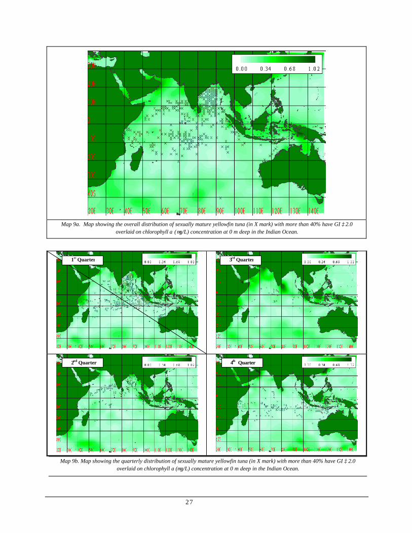
27

Map 9a. Map showing the overall distribution of sexually mature yellowfin tuna (in X mark) with more than 40% have GI ≥ 2.0

overlaid on chlorophyll a (µg/L) concentration at 0 m deep in the Indian Ocean.

Map 9b. Map showing the quarterly distribution of sexually mature yellowfin tuna (in X mark) with more than 40% have GI ≥ 2.0

overlaid on chlorophyll a (µg/L) concentration at 0 m deep in the Indian Ocean.

1st Quarter

4th Quarter 2nd Quarter

3rd Quarter

28

Figure 10.Map illustrating the bimonthly sampling coverage for yellowfin tuna larval survey.




29

Map 10a. Map showing the overall occurrence of yellowfin tuna larvae overlaid on the temperature (°C) profile at 0 m – 30 m deep

in the Indian Ocean.



30

Larval occurrence vs. salinity (0-30m)(Map 11)

Map 11a shows the overall occurrence of yellowfin tuna larvae overlaid on the salinity profile in the Indian Ocean. Yellowfin tuna larvae were found in waters with salinity ranging within and just above 32 psu, predominant in eastern and central Indian Ocean.

Map 11b shows the bimonthly occurrence of yellowfin tuna larvae overlaid on salinity profile in the Indian Ocean. Density of aggregation varies with season and independently from changing salinity profile.

Larval occurrence vs. oxygen concentration (0-30m) (Map 12)

Map 12a shows the overall occurrence of yell owfin tuna larvae overlaid on the dissolved oxygen profile in the Indian Ocean. Majority of the yellowfin tuna larvae occurred in oxygen rich waters ranging approximately in between 4.7 ml/L and 6.1 ml/L O 2.

Map 12b shows the bimonthly occurrence of yellowfin tuna larvae overlaid on the dissolved oxygen profile in the Indian Ocean. Oxygen rich waters prevailed almost in the entire Indian Ocean. The pattern of distribution vaguely followed the changes in oxygen profile. However, aggregation of larvae was never situated in waters with oxygen level below 4.7 ml/L O2.

Larval occurrence vs. chlorophyll (0-30m)(Map 13)

Map 13a shows overall occurrence of yellowfin tuna larvae overlaid on chlorophyll a concentration in the Indian Ocean. Generally, majority of

the yellowfin larvae was found in areas within chlorophyll a concentration ranging below 0.34 µg /L. Occurrence was also observed near high productive areas along the coast, surrounding the Bay of Bengal and western Sumatra. However, scattered occurrence could also be observed in less productive area like the dense aggregation off the northern coast of Australia.

Quarterly distribution (map 13b) showed a similar trend during the first quarter. Fewer occurrences were observed during the second and third quarter and regained intensity at the last quarter. Ironically, aggregation seemed intense during the lower chlorophyll concentration season (1st and 4th quarters) and less intense during high productive season (2nd and 3rd quarters).

Map 10b. Map showing the bimonthly occurrence of yellowfin tuna larvae (in X mark) overlaid on the temperature (°C) profile at 0

m – 30 m deep in the Indian Ocean.

Map 11a. Map showing the overall occurrence of yellowfin tuna larvae (in X mark) overlaid on the salinity (psu) profile at 0 m – 30 m deep in the Indian Ocean.


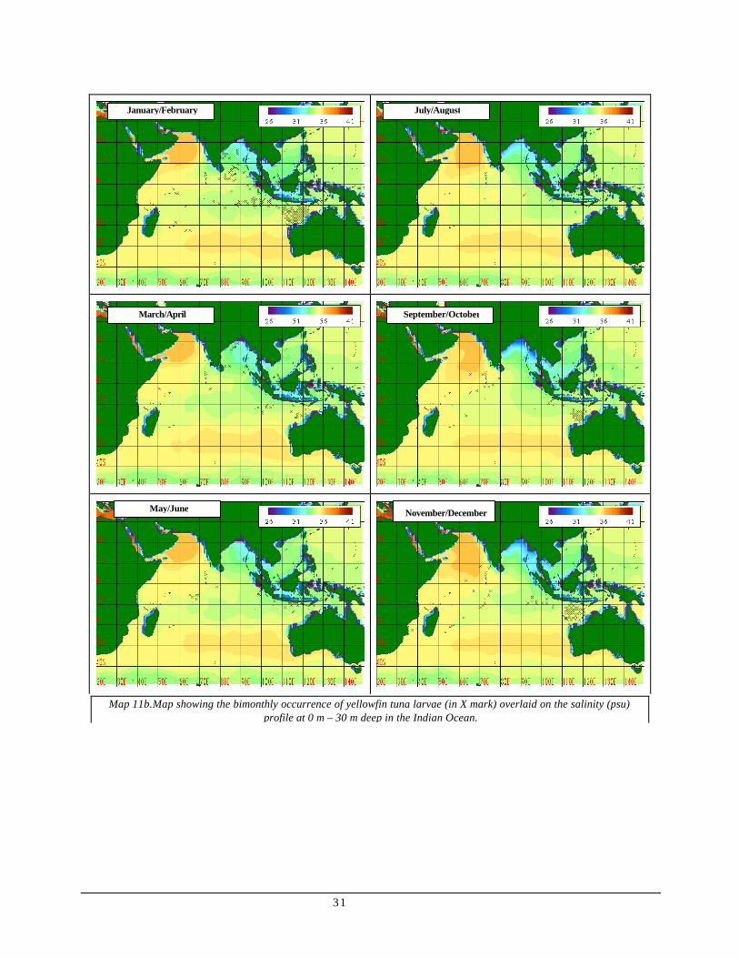
31

Map 11b.Map showing the bimonthly occurrence of yellowfin tuna larvae (in X mark) overlaid on the salinity (psu) profile at 0 m – 30 m deep in the Indian Ocean.



May/June November/December

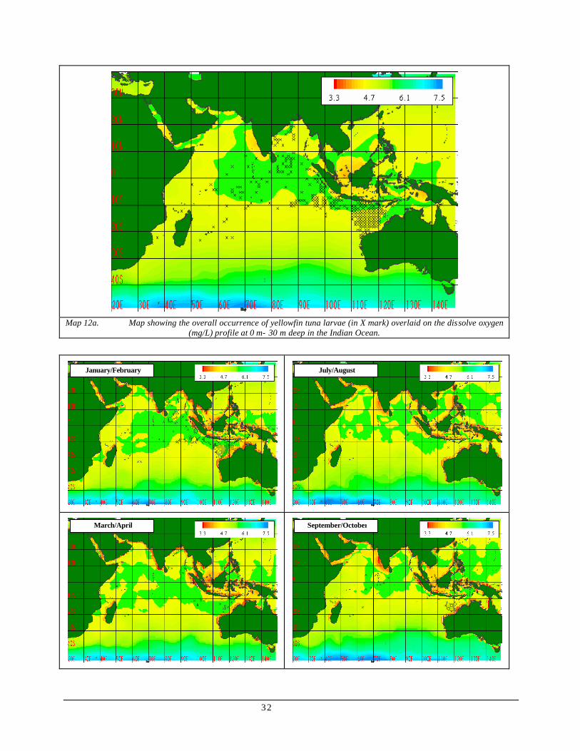
32

Map 12a. Map showing the overall occurrence of yellowfin tuna larvae (in X mark) overlaid on the dissolve oxygen

(mg/L) profile at 0 m- 30 m deep in the Indian Ocean.



33

Map 12b.Map showing the bimonthly occurrence of yellowfin tuna larvae (in X mark) overlaid on the dissolve oxygen

(mg/L) profile at 0 m -30 m deep in the Indian Ocean.

Map 13a.Map showing the overall occurrence of yellowfin tuna larvae (in X mark) overlaid on the isobath (m) of 20°C in

the Indian Ocean.



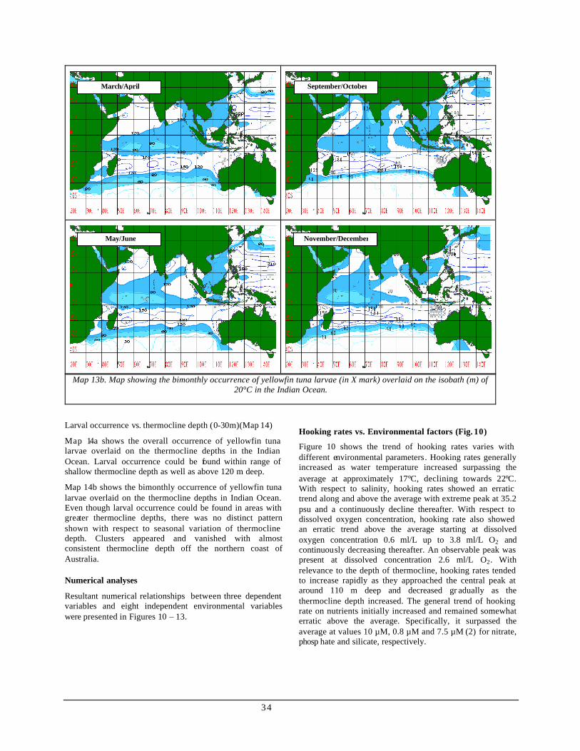
34

Map 13b. Map showing the bimonthly occurrence of yellowfin tuna larvae (in X mark) overlaid on the isobath (m) of

20°C in the Indian Ocean.

Larval occurrence vs. thermocline depth (0-30m)(Map 14)

Map 14a shows the overall occurrence of yellowfin tuna larvae overlaid on the thermocline depths in the Indian Ocean. Larval occurrence could be found within range of shallow thermocline depth as well as above 120 m deep.

Map 14b shows the bimonthly occurrence of yellowfin tuna larvae overlaid on the thermocline depths in Indian Ocean. Even though larval occurrence could be found in areas with greater thermocline depths, there was no distinct pattern shown with respect to seasonal variation of thermocline depth. Clusters appeared and vanished with almost consistent thermocline depth off the northern coast of Australia.

Numerical analyses

Resultant numerical relationships between three dependent variables and eight independent environmental variables were presented in Figures 10 – 13.

Hooking rates vs. Environmental factors (Fig. 10)

Figure 10 shows the trend of hooking rates varies with different environmental parameters. Hooking rates generally increased as water temperature increased surpassing the average at approximately 17°C, declining towards 22°C. With respect to salinity, hooking rates showed an erratic trend along and above the average with extreme peak at 35.2 psu and a continuously decline thereafter. With respect to dissolved oxygen concentration, hooking rate also showed an erratic trend above the average starting at dissolved oxygen concentration 0.6 ml/L up to 3.8 ml/L O2 and continuously decreasing thereafter. An observable peak was present at dissolved concentration 2.6 ml/L O2. With relevance to the depth of thermocline, hooking rates tended to increase rapidly as they approached the central peak at around 110 m deep and decreased gr adually as the thermocline depth increased. The general trend of hooking rate on nutrients initially increased and remained somewhat erratic above the average. Specifically, it surpassed the average at values 10 µM, 0.8 µM and 7.5 µM (2) for nitrate, phosp hate and silicate, respectively.



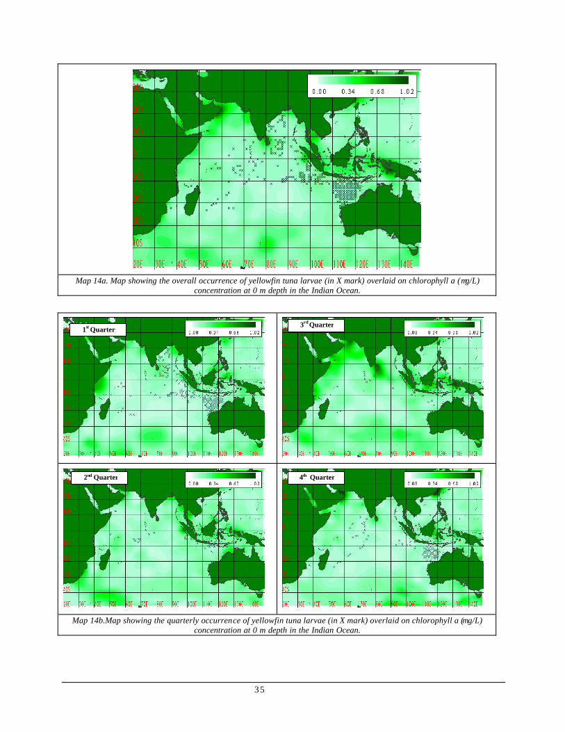
35

Map 14a. Map showing the overall occurrence of yellowfin tuna larvae (in X mark) overlaid on chlorophyll a (µg/L)

concentration at 0 m depth in the Indian Ocean.

Map 14b.Map showing the quarterly occurrence of yellowfin tuna larvae (in X mark) overlaid on chlorophyll a (µg/L) concentration at 0 m depth in the Indian Ocean.

1st Quarter

4th Quarter 2nd Quarter

3rd Quarter

36

Figure 11. Graphs showing the relationship between hooking rates and environmental parameters in the 50-200m depth range. The horizontal line represents the overall average (threshold value).

Hooking rate (HR) vs. nitrate concentration(n=9,944)

0

5

10

15

20

25

0 1 2 3 4 5 6 7 8 9 10 11 12 13 14 15 16 17 18 19 20 21 22 23 24

Nitrate (µM) concentration

Hoo

king

rate

(no.

of f

ish/

1000

hoo

ks)

Observed HRAverage HR

Hooking rate (HR) vs. phosphate concentration(n=9,928)

0

5

10

15

20

25

0.1 0.2 0.3 0.4 0.5 0.6 0.7 0.8 0.9 1 1.1 1.2 1.3 1.4 1.5 1.6 1.7 1.8

Phosphate (µM) concentration

Hoo

king

rate

(n

o. o

f fis

h/10

00 h

ooks

)


Hooking rate (HR) vs. silicate concentration(n=9,920)

0

2

4

6

8

10

12

14

16

18

20

1 3 5 7 9 11 13 15 17 19 21 23 25 27 29

Silicate (µM) concentration

Hoo

king

rate

(no.

of f

ish/

1000

hoo

ks)


Hooking rate (HR) vs. dissolve oxygen(n=23,204)

0

5

10

15

20

25

0.6 1 1.4 1.8 2.2 2.6 3 3.4 3.8 4.2 4.6 5 5.4 5.8 6.2

Dissolve oxygen (ml/L)

Hoo

king

rate

(n

o. o

f fis

h/10

00 h

ooks

) Observed HRAverage HR

Hooking rate (HR) vs Salinity(n=23,201)

0

5

10

15

20

25

34.2

34.3

34.4

34.5

34.6

34.7

34.8

34.9 35

35.1

35.2

35.3

35.4

35.5

35.6

35.7

35.8

35.9 36

36.1

36.2

Salinity (PSU)

Hoo

king

rate

(n

o. o

f fis

h/10

00 h

ooks

)


Hooking rate (HR) vs. depth of thermocline(n=17,700)

0

5

10

15

20

25

0 10 20 30 40 50 60 70 80 90

100

110

120

130

140

150

160

170

180

190

200

210

Depth (m) of thermocline at 20°C isotherm

Hoo

king

rate

(no.

of f

ish/

1000

hoo

ks)


Hooking rate (HR) vs. water temperature(n=23,200)

0

2

4

6

8

10

12

14

16

18

9 10 11 12 13 14 15 16 17 18 19 20 21 22 23

Temperature (°C)

Hoo

king

rate

(n

o. o

f fis

h/10

00 h

ooks

)

Observed HR

Average HR

37

Spawning activities vs. Environmental factors (Fig. 12)

Figure 12 shows the trend of the percentage of sexually mature yellowfin tuna expressed against environmental factors. Sexually mature yellowfin tunas were inclined towards warmer waters starting a rapid increase from 24oC, surpassing the average at 27°C and continuously increase thereafter. Preference on salinity, on the other hand, was strongly inclined with more than 60 percent at concentration starting 32.6 psu, increasing at 33 psu and decreasing rapidly thereafter. Percentage of sexually mature yellowfin tuna dropped below the average at 34.8 psu. With respect to dissolved oxygen concentration, percentage of sexually mature individual generally started off above the average at 4.0 ml/L O2 and continuously decreased after it reached a secondary peak at 4.5 ml/L O2. Percentage went below the average at 4.2 ml/L O2 and 4.7 ml/L O2 onwards. With respect to the depth of thermocline, sexually mature yellowfin tuna rapidly increased above average at thermocline depth of approximately 90 m and maintained a plateau up to 140 m deep where it began to decrease. With respect to chlorophyll a concentration, the percentage of sexually mature yellowfin tuna seemed erratic in between the 15 to 25 percent starting from 0.02 µg/L to 0.28 µg/L chlorophyll a concentration. While sexually mature yellowfin tunas generally increased with nutrient concentration. The percentage of sexu ally mature yellowfin tunas reached a peak of more than 60 percent at 3.5 µM nitrate concentration.

Larval distribution vs. Environmental factors (Fig. 13)

Figure 13 shows the trend of larval occurrence over a range of environmental parameters. Likewise, larval occurrences were inclined to warmer water temperature with abrupt increase starting 26°C to 29°C for which it remained at its highest occurrence. Preferential salinity peaked at 34.6 psu and continuously dropped to zero level with 35.4 psu. Larval

counts abruptly increased from 4.3 ml/L reaching its peak at around 4.5 ml/L dissolved oxygen concentrations where it decreased thereafter. With respect to thermocline depth, larval occurrences seem erratic initially. Then it increased starting at the depth of 120 m reaching its peak at 150 m where it was followed by an abrupt decrease at 160 m deep. With respect to chlorophyll a concentration, larval occurrence gradually increased, reaching its peak at 0.08 µg/L, followed by an abrupt decrease at 0.1 µg/L whereby it remained jagged below the average level. For nutrients, the larval occurrence showed a clear decreasing trend only with respect to nitrate with highest counts at zero nitrate concentration. Erratic patterns with extreme crest and trough were observed as a function of phosphate and nitrate concentration.

Spectra of optimum rage of Environmental factors

From the resultant graphs (Figures 12-13), the optimum range of environmental parameters that produce favorable hooking rates, spawning activities and larvae distribution (those values above the threshold values) were extracted and summarized in Table 4. Spectra of these optimum ranges were also depicted in Figure 14. Optimal water temperature for spawning adults and larvae were much higher than for adult yellowfin tunas. Optimal salinity for spawning adults, on the other hand, had a wider range, while larvae and adult yellowfin tunas were restricted to more saline waters. Optimal dissolved oxygen for common adults had a wider range than that for spawning adult and larvae, which were restricted to above 4.0 ml/L O2 concentration. Preferred thermocline depth of adult and larvae were on inverse partiality, the latter on the deeper side. Spawning adults, on the other hand, seemed to be in transition. Preferential chlorophyll a concentration for spawning adults had a wider range than that for the larvae, which was confined below 0.1 µg/L.

38

Figure 12.Graphs showing the relationship between the composition where ≥41% are sexually mature yellowfin tuna (YFT) and environmental parameter in the 0-50m depth range. The horizontal line represents overall average (threshold value).

Compostion of sexually mature YFT (%) vs. silicate concentration (n=3,558)

0

5

10

15

20

25

30

35

40

45

0 1 2 3 4 5 6 7 8 9 10 11

Silicate (µM) concentration

% o

f sex

ually

mat

ure

YF

Tw

ith G

I ≥

2.0

Observed %

Average %

Composition of sexually mature YFT (%) vs. phosphate concentration (n=3,562)

0

5

10

15

20

25

30

35

0 0.1 0.2 0.3 0.4 0.5 0.6


% o

f sex

ually

mat

ure

YF

Tw

ith G

I ≥

2.0

Observed %Average %

Composition of sexually mature YFT (%) vs. nitrate concentration (n=3,562)

0

10

20

30

40

50

60

70

0 0.5 1 1.5 2 2.5 3 3.5 4 4.5


% o

f sex

ually

mat

ure

YFT

w

ith G

I ≥

2.0

Observed %

Average %

Composition of sexually mature YFT (%) vs. Chlorophyll a (n=1,890)

0

5

10

15

20

25

0.02 0.04 0.06 0.08 0.1 0.12 0.14 0.16 0.18 0.2 0.22 0.24 0.26 0.28 0.3 0.32

Chlorophyll a concentration (µg/L) at water surface (0m)

% o

f sex

ually

mat

ure

YFT

with

GI

≥ 2

.0

Observed %Average %

Composition of sexually mature YFT (%) vs. depth of thermocline (n=4,520)

0

5

10

15

20

25

30

40 50 60 70 80 90 100 110 120 130 140 150 160 170 180 190 200

Depth (m) of thermocline at 20°C isotherm

% o

f sex

ually

mat

ure

YF

Tw

ith G

I ≥

2.0

Observed %

Average %

Composition of sexually mature YFT (%) vs. dissolved oxygen (n=5,425)

0

5

10

15

20

25

30

4 4.1 4.2 4.3 4.4 4.5 4.6 4.7 4.8 4.9 5 5.1 5.2 5.3 5.4 5.5

Dissolved oxygen (ml/L)

% o

f sex

ually

mat

ure

YF

T

with

GI

≥ 2.

0

Observed %

Average %

Composition of sexually mature YFT (%) vs. water temperature (n=5,439)

0

5

10

15

20

25

30

35

40

18 19 20 21 22 23 24 25 26 27 28 29 30

Temperature (°C)

% o

f sex

ually

mat

ure

YFT

with

GI

≥ 2.

0

Observed %Average %

Composition of sexually mature YFT (%) vs. salinity(n=5,436)

0

10

20

30

40

50

60

70

80

32.6

32.8 33 33

.233

.433

.633

.8 34 34.2

34.4

34.6

34.8 35 35

.235

.435

.635

.8 36

Salinity (PSU)

% o

f sex

ually

mat

ure

YF

T w

ith

GI ≥

2.0

Observed %Average %

39

Figure 13. Graphs showing the relationship between larval density and environmental parameters in the 0-30m depth

range. Horizontal line indicates the overall average (threshold value)

Larval density (LD) vs. phosphate concentration(n=210)

0

0.5

1

1.5

2

2.5

0.08 0.1 0.12 0.14 0.16 0.18 0.2 0.22


Num

ber o

f lar

vae

per t

ow

Observed LDAverage LD

Larval density (LD) vs. nitrate concentration(n=208)

0

0.5

1

1.5

2

2.5

3

3.5

4

4.5

0 0.1 0.2 0.3 0.4 0.5 0.6 0.7


Num

ber o

f lar

vae

per t

ow Observed LDAverage LD

Larval density (LD) vs. chlorophyll a(n=284)

0

0.5

1

1.5

2

2.5

3

3.5

4

0.04 0.05 0.06 0.07 0.08 0.09 0.1 0.11 0.12 0.13 0.14 0.15

Chlorophyll a concentration (µg/L)

Num

ber o

f lar

vae

per t

ow


Larval density (LD) vs. depth of thermocline(n=342)

0

0.5

1

1.5

2

2.5

3

60 70 80 90 100 110 120 130 140 150 160 170

Depth of thermocline (m) at 20°C isotherm

Larv

al c

ount

s


Larval density (LD) vs. dissolved oxygen(n=525)

0

0.5

1

1.5

2

2.5

3

4.3 4.4 4.5 4.6 4.7 4.8 4.9 5 5.1 5.2 5.3

Dissolved oxygen (ml/L)

Num

ber o

f lar

vae

per t

ow


Larval density (LD) vs. salinity(n=534)

0

0.5

1

1.5

2

2.5

3

34.2 34.4 34.6 34.8 35 35.2 35.4 35.6 35.8 36

Salinity (PSU)

Num

ber o

f lar

vae

per t

ow


Larval density (LD) vs. water temperature(n=534)

0

0.5

1

1.5

2

2.5

3

3.5

19 20 21 22 23 24 25 26 27 28 29 30

Temperature (°C)

Larv

al c

ount

s


Larval density (LD) vs. silicate concentration(n=210)

0

0.5

1

1.5

2

2.5

3

0.5 1 1.5 2 2.5 3 3.5 4 4.5

Silicate (uM) concentration

Larv

al c

ount

s


40

Table 4. Optimum range of oceanographic parameters that produce favorable hooking rates spawning activities and larvae distribution.

Dependent variables è Unit Hooking rates (**) (no. of fish/1000

hooks)

Spawning activities (%of mature YFT)

Larvae distribution (no. of larvae per sample)

Criteria (threshold value)

(*)

13.4 21.2 1.3

Depth range Deep (50-200m) Shallow (0-50m) Shallow (0-30m) Independent Parameters

Temperature

(oC) 17.0-20.5 Mo (n=23,200)

26.8-30.0 Mo (n=5,439)

27.5- Mo (n=534)

Salinity

(psu)

34.2-34.4 Mo (n=23,201)

32.6-34.7 Mo (n=5,436)

34.2-34.9 Mo (n=534)

Dissolved Oxygen

(ml/L)

0.6-1.7 & 2.1-3.9 Mo (n=23,204)

4.00-4.15 or 4.30-4.65

Mo (n=5,425)

4.4-4.7 Mo (n=525)

Depth of

thermocline(20oC)

(m) 75-130

Mo (n=17,700)

89-147

Mo(n=4,520)

128-157

Mo(n=342)

Chlorophyll

(µM)

NA 0.06-0.13 or 0.15-0.17

No (n=1,890)

0.055-0.090 No (n=284)

Nitrate

(µM

)

10-24

Q (n=9,944)

1.8-4.5

Q (n=3,562)

0-0.43

Q (n=208)

Phosphate

(µM)

0.8-1.4 & 1.6-1.8 Q (n=9,928)

0.33-0.60 Q (n=3,562)

0.080-0.175 & 0.185-0.210 Q (n=210)

Silicate

(µM

)

8-29

Q(n=9,920)

6-11

Q (n=3,558)

0.7-1.3 or 2.2-3.7

Q(n=210) (Abbreviations) Mo, Q or No: Time scales for the analyses were monthly (Mo), quarterly (Q)

or no time scale involved (No). n : Sample size NA : No analyses were conduced

Note (*) : Mean values were used as criteria that produce favorable vale of the dependent variables. Note (**) : 0 catch data in certain 1x1 degree grid area and month in analyzed (45) years were not used.

Part I Basic parameters

(Temperature)(oC) 17.0 17.5 18.0 18.5 19.0 19.5 2 0 .0 20.5 21.0 21.5 22.0 22.5 23.0 23.5 24.0 24.5 25.0 25.5 26.0 26.5 27.0 27.5 28.0 28.5 29.0 29.5 30.0

HR (50-200m)

Spawning (0- 50m)

Larvae (0- 30m)

(Depth of thermocline at 20oC)(m) 75 80 85 90 95 100 105 110 115 120 125 130 135 140 145 150 155 160

HR (50-200m)

Spawning (0-50m)

Larvae (0-30m)

41

(Salinity)(psu) 32.6 32.7 32.8 32.9 33.0 33.1 33.2 33.3 33.4 33.5 33.6 33.7 33.8 33.9 34.0 34.1 34.2 34.3 34.4 34.5 34.6 34.7 34.8 34.9 35.0 35.1 35.2 35.3

HR (50-200m)

Spawning (0- 50m)

Larvae (0- 30m)

(Dissolved oxygen) (ml/L) 0.6 0.8 1.0 1.2 1.4 1.6 1.8 2.0 2.2 2.4 2.6 2.8 3.0 3.2 3.4 3.6 3.8 4.0 4.2 4.4 4.6 4.8 HR (50-20m)

Spawning (0-50m)

Larvae (0-30m)

(Chlorophyll)(µg/L) 0.05 0.06 0.07 0.08 0.09 0.10 0.11 0.12 0.13 0.14 0.15 0.16 0.17 HR (NA) (50-200m)

Spawning (0-50m)

Larvae (0-30m)

(NA) : Not available Figure 14.Optimum spectra of various oceanographic condition that produced favorable hooking rates (HR), spawning

activ ities and larvae distribution.

Part (II) Nutrients

(Phosphate ) (µM) 0.1 0.2 0.3 0.4 0.5 0.6 0.7 0.8 0.9 1.0 1.1 1.2 1.3 1.4 1.5 1.6 1.7 1.8 HR (50-200m)

Spawning (0-50m)

Larvae (0-30m)

(Silicate) (µM) 0 1 2 3 4 5 6 7 8 9 10 11 12 13 14 15 16 17 18 19 20 21 22 23 24 25 26 27 28 29 HR (50-200m)

Spawning (0- 50m)

Larvae (0- 30m)

(Nitrate ) (µM) 0 1 2 3 4 5 6 7 8 9 10 11 12 13 14 15 16 17 18 19 20 21 22 23 24 HR (50-200m)

Spawning (0-50m)

Larvae (0-30m)

Figure 14. (cont’d)

42

DISCUSSION

Obscure to many, virtually all problems have a spatial dimension (Maeden, 1996). Method and analysis were made possible through the use of georeferenced Japanese longline fisheries information and NODC's oceanographic surveys. However, it is also important to consider good data qu ality as provided by above mentioned databases in order to ensure reliable results of analyses for interpretation.

Distribution of adult YFT

The results of the qualitative analyses suggest that the adult yellowfin tuna distribution follow the spatial and seasonal changes of water temperature profile in the Indian Ocean. Combined with numerical analyses, results showed that the preferential water temperature lies within the optimum range from 17°C to 24°C.

Capability of body thermoregulation among adult yellowfin tuna explains the tolerance to lower optimum water temperature range. Stequert (1989) cited that older individuals penetrate deeper and colder waters than juveniles.

Explanation on spatial variation as influenced by temperature may not be straightforward. Hunter (1986) described the concept of limits based from correlation between tuna catches and the physical environmental barriers indicated by temperature. However, he mentioned that this concept is not supported by laboratory work, as there are instances that exceed beyond the thermal barriers. Kumari (1993), on the other hand, suggested that the abundance of tuna, in general, within the preferential temperature range was indirectly related to the presence of tuna forage brought about by physical processes such as fronts. Nonetheless, results depicted in thematic maps did not elucidate association between thermal fronts and tuna abundance because the analyses were not meant for such detailed scrutiny, though it poses an interesting subject for future studies.

Resulting preferential water temperature, on the other hand, coincides with previous findings of Nair (1993) and Mohri (2000a).

Though adult yellowfin tuna was fairly distributed within areas with high salinity, qualitative analysis failed to show clear spatial relationship. Numerical analysis indicated an optimum range from 34.2 to 34.4 psu and 35 to 35.3 psu. These findings suggest that salinity had less influence on the distribution because no steady salinity range produced high hooking rates. The optimum range, on the other hand, may only describe their oceanic habitat that could provide an indirect explanation on their abundance.

The results of the qualitative analyses on distribution and dissolved oxygen suggest a spatial and seasonal relation between the two. However, numerical analysis indicated a wider optimum range, from very minimal concentration of 0.6 ml/L O2 to 3.8 ml/L O2. The findings imply that yellowfin tuna preferred but were not limited to areas with

an optimal dissolved oxygen concentration. More over, the bulk of aggregation was less apparent in areas with 0.6 ml/L O2 concentration. In fact, the resulting sample size found at the lower concentration was low. Values depicted in the results were not comparable with the threshold value suggested by Mohri (2000) because his study was focused on evaluating the minimum oxygen level while this study was based on a general distribution.

Though vaguely shown, results of the qualitative analyses suggest an association between the distribution of adult yellowfin tuna and the thermocline depth, especially the observable affinity of dense aggregation within shallow thermocline depth. Numerical analysis, on the other hand, depicted a wide optimum range from 75 m to 130 m, with a central tendency around 100 m deep.

These results confirmed John’s (1995) findings that the thermocline depth had a negative influence on hooking rates. After the central peak around 100 m deep, hooking rate continued to decline with increasing thermocline depth. Though these values could not ascertain if yellowfin tuna have preferential thermocline depth, it may be a good indicator of hydrological condition. A deeper thermocline may indicate a convergence zone, while the opposite for divergence. With respect to areas of convergence and divergence, the observable shallow thermocline depth found just above 10o S latitude in western Indian Ocean, can be compared to the divergence zone from December to July. In coherence, the cluster of high hooking rates appeared to be denser during the same period at the same location. Though vaguely depicted in the result, the area of convergence, with high hooking rate density, lies just above and adjacent to this shallow thermocline depth. Hunter (1986), in his publication, reasons out that this observation is related to areas of productivity. Divergence is an area associated with high primary productivity due to the rising up of nutrient rich deeper water known as upwelling. Consequently, grazers and prey fishes take advantage of food available. However, physical processes of convergent zone in proximity accumulate the laterally dispersed organisms thus, the potential abundance of tunas in this area.

Another circumstance that supports high abundance in convergence zones is the consistent presence of aggregation in the Mozambique Channel from January to August and the reduction during September to December. The presence and absence of aggregation coincides with the periodicity of convergence in the region.

Also, an observable aggregation in the western Indian Ocean is evidently situated along the wider isobath intervals while scarce in narrow ones. This observation may imply that yellowfin tuna prefer the zones with minimal difference in thermocline depth. However, no vertical profile has been analyzed to ascertain the claim. Nonetheless, this assumption may agree with John (1995) finding that hooking rate is negatively related to isotherm depth and positively related to thermal gradient as depicted in Figure 15.

43

Though there are no maps to show the spatial relation between yellowfin tuna distribution and nutrient concentration, the numerical analysis showed that the optimum range for nitrate concentration is 10 µM to 24 µM; phosphate is 0.8 µM to 1.8 µM; and silicate is 8 µM to 29 µM. These values reflect the typical nutrient profile of the oceanic water column based on surveys conducted in Geochemical Ocean Sections Study (GEOSECS). Nutrient concentration increases with depth, reaching a certain point where concentration is almost constant. However, there is an argument that such parameters are also indicator of yellowfin tuna abundance. Nutrients are absorbed by primary producers which are then grazed upon by secondary producer (zooplanktons), eaten by small fishes and finally preyed upon by predators such as yellowfin tuna. Though Roger (1993) indicated in his study that there is an immediate link between plankton, plankton feeding prey-fishes and tuna, there is no illusive study that could support the argument. More so because his study was limited to surface tunas. In fact, complexities in the trophic pathways should be taken into account. The classical foodchain depicted above may not be true in all forms, especially in a marine ecosystem. The network of producers, consumers and decomposers creates a food web (Kiorbae, 1993; Legendre and Rassoulzadegan, 1995). Perhaps, it would be an interesting prospect to study spatial correlation between nutrient concentration, phytoplankton, grazers, prey-species and yellowfin tuna distribution without bypassing one or more trophic levels.

Spawning activities

In order to have comparable results, it is important to consider a consistent sampling strategy. Patchiness in sampling coverage poses discrepancies and may affect the reliability of information produced. For this study overall sampling coverage was extensive enough but for the bimonthly sampling patchiness was observed especially in the western Indian Ocean during some of the months. Hence, results should be interpreted cautiously.

The majority of the studies on spawning activities of yellowfin tunas have been focused on seasonal variation. Only in rare circumstances where spawning activities are related to environmental conditions such as water temperature.

Results of the qualitative analysis imply that there is a spatial and seasonal relation between the distribution of spawners and water temperature. Spawners are strongly inclined to warmer water temperature with optimum range of 26.5°C to 30°C.

The optimum range agreed with the findings of Shun g (1973) that the sexual activity of yellowfin tunas caught by longline fishery in the Indian Ocean advances at a temperature of 26°C and greater. But, he also pointed out that these advances might not be dependent on temperature alone.

Results from the qualitative analyses suggest that spawning activity had no clear spatial relation with salinity. However, the numerical analysis revealed that spawners are found in a wider optimum range of 32.6 psu to 34.7 psu, which is less than that for none spawning adults. Since the majority of the spawners aggregate in eastern Indian Ocean and the Bay of Bengal, their habitat is subject to lower salinity due to freshwater inflow from three major rivers namely, Irrawaddy River which discharges in the Andaman Sea while, Brahmaputra and Ganga Rivers discharges in the Bay of Bengal.

Results of the qualitative analysis suggest that there is spatial relation between spawning activity and dissolved oxygen concentration. The optimum range for dissolved oxygen concentration is 4.0 ml/L to 4.6 ml/L O2. These values coincide with ranges cited by Stequert (1989) and threshold values proposed by Cayre (1993).

Spatial correlation implies that optimum oxygen concentration is crucial to the spawning activity. Biological condition during reproductive development may pose changes in physiological needs. Hence, preferential habitat differentiates from ordinary non-spawning yellowfin tuna. However, this claim should be supported by laboratory experiment.

Results do not show a spatial relation between spawning activity and thermocline depth. More over, spawners were abundant at the optimum range from 90 m to 150 m. Unlike in the case of non-spawning adults, this findings implies that there are other factors more influential than what the thermocline depth may indicate. Perhaps, this is due to physiological needs.

The results of the qualitative analyses showed no clear spatial relation between chlorophyll a concentration and spawning activity. However, it is noteworthy to mention that intensity of spawning activity is low during high productive season and vice versa. Nonetheless, the optimum range is 0.6 µg/L to 0.17 µg/L chlorophyll a concentration. The time lag between intense aggregation and period of high productivity may indicate strategy of the population to attain equilibrium as influence of the environmental condition. However, this concept is remote from what is indicated by low optimal chlorophyll a concentration. A possible explanation is the oligotrophic characteristic of tropical open ocean (Thurman, 1996). Though light is not a limiting factor in primary productivity, tropical oceans have permanent thermocline that produces stratification of water masses where by mixing is prevented between surface waters and nutrient-rich deeper waters. Murty (2000) studied chlorophyll maximums in the Bay of Bengal. He revealed that a chlorophyll maximum is found in depths 50–100 m at open sea.

The numerical analysis shows an optimum range for nitrate concentration have 2 µM to 5 µM; for phosphate from 0.3 µM to 0.6 µM; and for silicate 6 µM to 11 µM. The values presented also describes the typical nutrient profile oceanic water column, especially at near surface. Phytoplanktons abound near surface water column for sunlight and utilize available nutrient in this layer. Hence, eutrophication leads

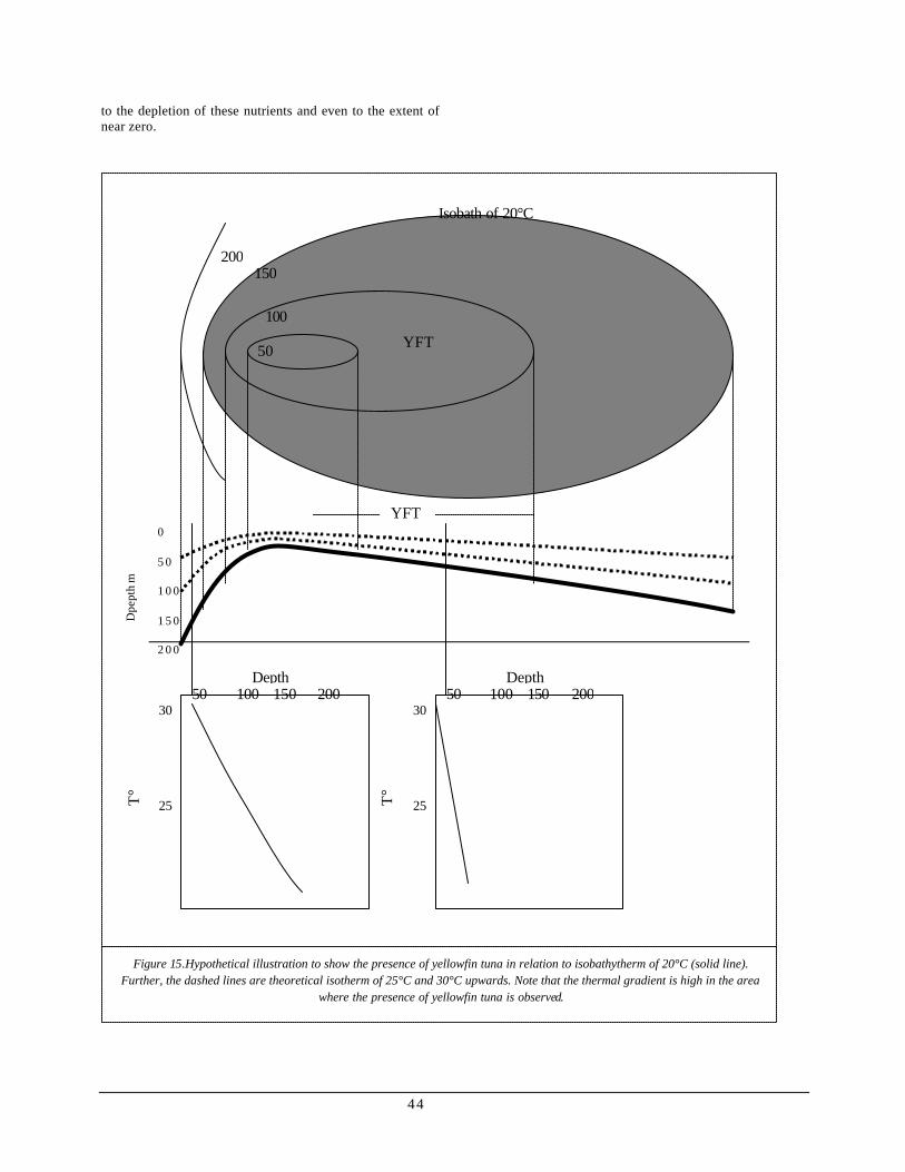
44

to the depletion of these nutrients and even to the extent of near zero.

YFT

Isobath of 20°C

T°

Depth 50 100 150 200

30 25

T° C

Depth 50 100 150 200

30 25

0

5 0

1 0 0

1 5 0Dpe

pth

m

2 0 0

YFT

200 150

100

50

Figure 15.Hypothetical illustration to show the presence of yellowfin tuna in relation to isobathytherm of 20°C (solid line). Further, the dashed lines are theoretical isotherm of 25°C and 30°C upwards. Note that the thermal gradient is high in the area

where the presence of yellowfin tuna is observed.

45

LARVAL OCCURRENCE

Likewise for larval data, sampling coverage is extremely patchy especially in the western Indian Ocean for both overall and bimonthly. This may be a possible explanation why most of the spatial analysis showed no respond, even though, areas near Sumatra and northwest of Australia were sampled considerably all year round.

Results of the qualitative analysis did not show a clear spatial relation between larval distribution and the temperature profile. However, the numerical analyses suggests that larvae are inclined towards warmer water temperature with an optimum range of 27.5°C to 30°C. This range agreed with the findings of Boehlert (1994) a temperature range greater than 24°C .

Results of the qualitative analysis did not show a clear spatial relation between larval distribution and salinity. The numerical analysis, however, showed that larvae were restricted towards higher salinity with an optimum range at 34.2 psu to 34.9 psu. A possible explanation for larval inclination to higher salinity is the role of viscosity on larval buoyancy. In the open ocean, temperature and salinity are two variables that affect viscosity (Thurman, 1996). Lower water temperature makes the water more viscous and inverse with salinity. Consequently, higher viscosity means greater buoyancy. Though temperature has a greater effect, salinity may pose more influence because of larval inclination to warmer waters. Hence, higher salinity facilitates in keeping yellowfin tuna larvae free floating.

Although results from qualitative analysis do not show a clear spatial relation between larval distribution and dissolved oxygen concentration, larvae are inclined towards high dissolved oxygen concentration. Optimum range depicted is at 4.4 ml/L to 4.8 ml/L O2. The findings exemplify the typical oxygen profile in open ocean as depicted in GEOSECS survey (Ross, 1988). Higher oxygen concentration is observed near water surface and decreases with depth until it reaches a minimum where it begins an almost constant profile.

Qualitative analyses did not show a clear spatial relation between larval distribution and depth of the thermocline. However, larvae were concentrated in areas with greater thermocline depth with optimum range at 130 m to 160 m deep.

The results of the numerical analyses imply that deeper thermocline depth favors larval survival on three counts. First, a deeper thermocline depth has a wider the mixed surface layer which creates a steady and rich environment. Second, a deeper thermocline also creates a wider water column with less thermal difference. Due to their undeveloped thermal regulatory system at this stage, larvae are not subject to abrupt changes in water temperature. Third, though remotely related, is the absence or lower density of adult yellowfin tuna in these areas that will somehow limit predation.

Results of the qualitative analyses do not show spatial relation between larval distribution and chlorophyll a concentration. Numerical analyses show that larvae are inclined at chlorophyll concentration at an optimum range of 0.05 µg/L to 0.09 µg/L. Though there is no apparent influence shown by the results, aggregation in the water northwest of Australia coincides with high zooplanktonic biomass present in these areas from August to September and February to March. Even though there are overlaps in time, intensified larval aggregation during the last and first quarter of the year may suggest that larvae opt to be influence by food availability. Further, it ensures higher survival rates even if spawning is assumed all year round. However, this speculative thought needs to be verified.

Numerical analyses showed that larval distribution are concentrated in areas where nutrient concentrations are extremely low to negligible. This is a typical chlorophyll a concentration at depth 0–30 m. As mentioned above, nutrient concentration at near surface water column may be depleted due to primary productivity.

No spatial correlation implies that distribution of yellowfin tuna larvae seemed to be influenced by environmental factors other than the above mentioned. Boehlert (1994) suggests that tuna larval distribution is initially established from spawning and dispersion by passive processes dependent on larval buoyancy. Highest aggregation density of spawners and larvae in the eastern Indian Ocean during January/February seemed to be coherent with his findings. He also mentioned that yellowfin tuna larvae had an affinity to land. This seems evident in the aggregation northwest of Australia and along the coast of Sumatra. However, there are also occurrences in mid -eastern Indian Ocean.

Migration

Expansion and constriction of high hooking rate aggregation suggest movement of yellowfin tuna with respect to environmental parameters. Yellowfin population may seem to be one homogenous stock located in the mid-western Indian Ocean. Based on changes in optimum environmental range indicated by temperature and oxygen, the population tends to spread out, going to the eastern Indian Ocean up to Bengal Bay and constrict after some time. As opposed to the findings of Nishida (1992) that there are two major yellowfin tuna stocks in the Indian Ocean, the homogeneity of the yellowfin population depicted in the result is not a good indicator for stock delineation. It is rather to illustrate the effect of environmental effect on the distribution.

Morhi (2000b) discussed the horizontal movement of yellowfin tuna in the Indian Ocean using longline catch data. His findings revealed that there is a distinct separation between the western and eastern high -fishing density area. The findings of this study do not show the same trend. Though he also identified that the center of high density fishing is located northern of Madagascar Island, this study found that the bulk of high hooking rate includes the same location but extends up to 80°E with some aggregation also found in the Sri Lanka’s coast, the Andaman Islands and south of Java. Unlike his findings, there was no profound

46

bulk in the north of Australia. Expansion in the western Indian Ocean coincides with the spread of high hooking rate during January to April and retracts from May to October. However, taking the Indian Ocean as a whole, retraction was only evident in the Arabian Sea and simultaneous expansion towards the eastern Indian Ocean reaching Bay of Bengal was evident during May/June. Further, there was no evident expansion in so called eastern area. In general, the finding of this paper does not delineate the yellowfin tuna population between western and eastern areas. The center of high density is located along Mozambique Channel and the area 0° to 10°S and 40°E to 80°E. Expansion occurred starting January to June moving northward and eastward. Lesser density was observed starting July to October especially in the Bay of Bengal, but no constriction was observed because aggregation remained along the equatorial region. Constriction is evident on November/December, when the high density in the aforementioned area is rebuilding in dense aggregation.

Homogeneity of the population in the Indian Ocean seemed to be evident, based on the spatial and temporal differences in aggregation of spawning and non-spawning adult yellowfin tuna. High Hooking rates as indicator of non-spawning adult is centralized in the western Indian Ocean, whereas sexually mature individuals are predominant in the eastern Indian Ocean. The first six months of the bimonthly profiles showed an observable progression of the displacement in areas of dominance between the two. In January, high hooking rates are predominant in the western side reaching up to the Arabian Sea but rare in the eastern side. While, sexually mature individuals are predominant in the eastern side reaching up to the Bay of Bengal. As the months advance, spawning adults in the eastern side diminish, while high hooking rates become denser in the eastern side. By May and June, high hooking rates prevail in both areas and spawning adults are scarce. This suggests that the expansion in the eastern portion is a movement of spawning adult eastward. Rare high hooking rates during peak spawning activity may just indicate lesser vulnerability of spawning adult to longline fisheries because it is presumed that they also move towards the surface during this period. The prevalence of high hooking in May and June, indicates that spawning activity is over and the fishes are going back to their regular habitat, which increases their vulnerability to longline fisheries. The second half indicates retraction to the western portion, where they start to become denser in November and December, to start the cycle.

CONCLUSION

The study demonstrates the use of secondary data that have been compiled for several decades by different sources and disciplines. Fisheries biologists and oceanographers are continuously collecting data with increasing efficiency in time. Coupled with advancing technology such as GIS, analyses using similar methods in this study profess a potential future. Perhaps this approach could be used, not just consolidating two disciplines but also others as well such economics and social sciences.

Though the approach is generally extensive, this is one of the first studies that has carried out analyses for three life stages of yellowfin tuna simultaneously relating it to depth specific five environmental factors in the Indian Ocean. Since the marine environment has a lot of interdependent factors, it will also be important to consider other factors such as bait, current and monsoon, which are of future concerns .

In spite of the fact that no statistical tests were attempted, results of this study suggest that various environmental factors are important to different life stage of yellowfin tuna.

For the distribution of adult yellowfin tuna, environmental variables namely water temperature, dissolved oxygen concentration and thermocline depth manifested direct influences. While, there are also indirect or less influential factors such as thermal fronts, thermal gradient and areas of convergence.

Temperature and dissolved oxygen concentration are the major factors that affect spawning activity.

For larval distribution, temperature, dissolved oxygen and thermocline depth are important factors.

It is further recommended to: 1 Conduct statistical tests to ascertain the findings

above and determine its significance.

2 Conduct further study in a smaller time scale than

using the totality of decades of data.

3 Consider other factors that may have potential

effect to yellowfin tuna distribution such as baits,

monsoon, physical processes and food abundance.

47

REFERENCES

ALTRINGHAM , JOHN D. AND BARBARA A. BLOCK. 1997. Why do tuna maintain elevated slow muscle temperatures? Power output of muscle isolated from endothermic and Ectothermic fish. The Journal of Experimental Biology 200:2617–2627.

ARDILL, J. D., (EDITOR). 1994. Proceedings of the expert consultation on Indian Ocean Tunas, 5th Session, Mahe, Seychelles, 4-8 October, 1993. IPTP Collective Volumes 8:275p.

BLOCK, B. A., J. E. KEEN, B. CASTILLO, E. V. FREUND, D. M. MARCINEK, R. W. BRILL AND C. FARWELL . 1997. Environmental preferences of yellowfin tuna (Thunnus albacares) at the northern extent of its range. Marine Biology 130:119-132.

BOEHLERT, GEORGE W. AND BRU CE C. MUNDY. 1994. Vertical and onshore-offshore distributional patterns of tuna larvae in relation to physical habitat features. Marine Ecology Progress Series, vol. 107:1-13.

BRILL, R. W., B. A. BLOCK, C. H. BOGGS, K. A. BIGELOW, E. V. FREUND AND D. J. MARCINEK. 1999. Horizontal movements and depth distribution of large adult yellowfin tuna (Thunnus albacares) near the Hawaiian Islands, recorded using ultrasonic telemetry: implications for the physiological ecology of pelagic fishes. Marine Bilology. 133:395-408.

CAYRE, P ATRICE AND FRANCIS MARSAC. 1993. Modelling the yellowfin tuna (Thunnus albacares) vertical distribution using sonic tagging results and local environmental parameters. Aquatic Living Resources 6: 1-14

DEWAR, H., J.B. GRAHAM AND R.W.BRI LL. 1994. Studies of tropical tuna swimming performance in a large water tunnel. II Thermoregulation. Journal on Experimental Biology 192:33-44.

ENVIRONMENTAL SIMULATION LABORATORY IN C. 2000. Manual on marine explorer ver. 3.07. 136p.

FROESE, R. AND D. PAULY. EDITORS. 2000. FishBase. World Wide Web electronic publication. www.fishbase.org, 16 August 2000

HUNTER, J., A. W. ARGUE, W. H. BAYLIFF, A.E. DIZON, A. FONTENEAU, D. GOODMAN AND G. R. SECKEL. 1986. The dynamics of tuna movements: an evalutation of past and future research. FAO Fisheries technical paper no. 277. Rome, Italy. FTP 277:23-33.

HUNTER, JOHN R., A. W. ARGUE, WILLIAM H. BAYLIFF, ANDREW E. D IZON, ALAIN FONTENEAU, DANIEL GOODMAN AND GUNTER R. SECKEL. 1986. The dynamics of tuna movements: an evaluation of past and future research. FAO Technical paper 277. Rome, Italy. FTP277:23-33.

JOHN, M.E. 1995. Some observations on the role of thermal processes on distribution of yellowfin tuna with refernece to longline fishing. Anganuzzi, A.A., K. A. Stobberup and N. J. Webb (eds).Proceedings of the expert consultation on Indian Ocean tunas, 6th session, Colombo, Sri Lanka. 136p.

KAJI, T ATSUYA, MASARU T ANAKA AND MASATOMO T AGAWA. 1999. Laboratory study of de nsity-dependent survival after handling in yolk-sac larvae of tunas and a grouper. Fisheries science. Tokyo. 65/3:482-483.

KIORBAE, T. 1993. Turbulence, phytoplankton cell size and the structure of the pelagic food chain. Adv.in Mar. Biol. 29:1-72.

KOIDO, TAKASHI. 1985. Comparison of fishing efficiency between regular and deep longline gears on bigeye and yellowfin tunas in the Indian Ocean. 1s t Expert consultation on stock assessment of tunas in the Indian Ocean, Colombo, Sri Lanka, 28 Nov – 2 Dec., 1985. Collective volume of working document. IPTP TWS/85/25:62-70.

KORSMEYER, KEITH E., N. CHIN LAI, ROBERT E. SHADWICK AND JEFFREY B. GRAHAM. 1997. Oxygen transport and cardiovascular responses to exercise in the yellowfin tuna Thunnus albacares. The Jour nal of Experimental Biology 200:1987–1997.

KUMARI, BEENA, M INI RAMAN, A. NARAIN AND T. E. SIVAPRAKASAM. 1993. Satellite remote sensing for tuna fishing in Indian waters. Sudarsan, D. and M. E. John, (eds). Tuna research in India.157-166 pp.

LEGENDRE, L. AND RASSOULZADEGAN. 1995. Plankton and nutrient dynamics in marine waters. Ophelia, 41:153-172.

MARSAC, FRANCIS AND PATRICE CAYRE. 1998. Telemetry applied to behaviour analysis of yellowfin tuna (Thunnus albacares, Bnnaterre, 1788) movements in a network of fish aggregating devices. Hydrobiologia. 371/372:155-171.

MOHRI, MASAHIKO. 1998. Distribution of bigeye tuna in the Indian Ocean based on the Japanese tuna longline fisheries and survey information. Ph.D. Thesis, National Fisheries University, Japan. 138p.

MOHRI, MASAHIKO . 2000a. Distribution of fishing of yellowfin tuna in the Indian Ocean – relations between water temperature and dissolved oxygen amount. (unpublished)

MOHRI, MASAHIKO, 2000b. Yellowfin tuna fishing distribution in the Indian Ocean – examination from horizontal and vertical direction. (unpublished)

MURTY, V. S. N., G. V. M. GUPTA, V. V. SARMA , V. V. RAO, D. JYOTHI, P. N. M. SHASTRI AND Y SUPRAVEENA. 2000. Effect of vertical stability and circulation on the depth of the chlorophyll maximum in the Bay of Bengal during May—June, 1996. Deep-Sea Research (Part 1, Oceanographic Research Papers) vol. 47, no. 5:859-873

NAIR, K. N. V. AND P. M. MURALEEDHARAN. 1993. Pattern of spatial and seasonal fluctuations in temperature profile in Indian EEZ and its influence on tuna fishing. Sudarsan, D. and M. E. John, (eds). Tuna research in India. 167-179.

NISHIDA, TSUTOMU. 1992. Considerations of stock structure of yellowfin tuna (Thunnus albacares) in the Indian Ocean. Fisheries Oceanography, vol. 1, no. 2:143-152

48

ROGER, CLAUDE. 1994. On feeding conditions for surface tunas (yellowfin, Thunnus albacares and skipjack, Katsuwonus plamis) in the western Indian Ocean. Ardill, J. D. (ed), Proceedings of the expert consultation on Indian Ocean Tunas, 5th Session, Mahe, Seychelles, 4-8 October, 1993. IPTP Collective Volumes 8:131-134.

ROSS, DAVID A. 1988. Introduction to Oceanography 4 th edition. Prentice Hall. New Jersey, USA. 478p.

SHUNG, SHING-HWA. 1973. The sexual activity of yellowfin tuna caught by the longline fishery in the Indian Ocean based on the examination of ovaries. Bulletin Far Seas Fisheries Res. Lab., no. 9:123-142.

STEQUERT, B. AND F. M ARSAC. 1989. Tropical tuna – surface fisheries in the Indian Ocean. FAO Fisheries technical pap er no. 282. Rome, Italy. FPT 282:7-77.

SUZUKI, Z IRO . 1994 A review of the biology and fisheries for yellowfin tuna ( Thunnus albacares) in the western and central Pacific Ocean. R. S. Shomura, J. Majkowski and S. Langi (eds). Interactions of Pacific tuna fisheries. FAO technical paper no. 336. Rome Itally. FTP 336:128-120.

THURMAN, HAROLD. 1996. Essentials of oceanography 5 th edition. Prentice hall. New Jersey, USA. 399p

TIMOCHINA, O. I. AND E. V. ROMANOV. 1991. Notes on reproductive biology of yellowfin tuna in the western Indian Ocean. IPTP. Collective Volume of Working Document 6. TWS/91/32:60-69.

factors affecting di stribution of adult … filefactors affecting di stribution of adult yellowfin...

Documents