Factorial, Gamma and Beta Functions

Reading Problems

Outline

Background . . . . . . . . . . . . . . . . . . . . . . . . . . . . . . . . . . . . . . . . . . . . . . . . . . . . . . . . . . . . . . . . . . . 2

Definitions . . . . . . . . . . . . . . . . . . . . . . . . . . . . . . . . . . . . . . . . . . . . . . . . . . . . . . . . . . . . . . . . . . . . . 3

Theory . . . . . . . . . . . . . . . . . . . . . . . . . . . . . . . . . . . . . . . . . . . . . . . . . . . . . . . . . . . . . . . . . . . . . . . . . 5

Factorial function . . . . . . . . . . . . . . . . . . . . . . . . . . . . . . . . . . . . . . . . . . . . . . . . . . . . . . . 5

Gamma function . . . . . . . . . . . . . . . . . . . . . . . . . . . . . . . . . . . . . . . . . . . . . . . . . . . . . . . . 7

Digamma function . . . . . . . . . . . . . . . . . . . . . . . . . . . . . . . . . . . . . . . . . . . . . . . . . . . . . 18

Incomplete Gamma function . . . . . . . . . . . . . . . . . . . . . . . . . . . . . . . . . . . . . . . . . .21

Beta function . . . . . . . . . . . . . . . . . . . . . . . . . . . . . . . . . . . . . . . . . . . . . . . . . . . . . . . . . . . 25

Incomplete Beta function . . . . . . . . . . . . . . . . . . . . . . . . . . . . . . . . . . . . . . . . . . . . . 27

Assigned Problems . . . . . . . . . . . . . . . . . . . . . . . . . . . . . . . . . . . . . . . . . . . . . . . . . . . . . . . . . . 29

References . . . . . . . . . . . . . . . . . . . . . . . . . . . . . . . . . . . . . . . . . . . . . . . . . . . . . . . . . . . . . . . . . . . . 32

1

Background

Louis Franois Antoine Arbogast (1759 - 1803) a French mathematician, is generally creditedwith being the first to introduce the concept of the factorial as a product of a fixed numberof terms in arithmetic progression. In an effort to generalize the factorial function to non-integer values, the Gamma function was later presented in its traditional integral form bySwiss mathematician Leonhard Euler (1707-1783). In fact, the integral form of the Gammafunction is referred to as the second Eulerian integral. Later, because of its great importance,it was studied by other eminent mathematicians like Adrien-Marie Legendre (1752-1833),Carl Friedrich Gauss (1777-1855), Cristoph Gudermann (1798-1852), Joseph Liouville (1809-1882), Karl Weierstrass (1815-1897), Charles Hermite (1822 - 1901), as well as many others.1

The first reported use of the gamma symbol for this function was by Legendre in 1839.2

The first Eulerian integral was introduced by Euler and is typically referred to by its morecommon name, the Beta function. The use of the Beta symbol for this function was firstused in 1839 by Jacques P.M. Binet (1786 - 1856).

At the same time as Legendre and Gauss, Cristian Kramp (1760 - 1826) worked on thegeneralized factorial function as it applied to non-integers. His work on factorials was in-dependent to that of Stirling, although Sterling often receives credit for this effort. He didachieve one “first” in that he was the first to use the notation n! although he seems not tobe remembered today for this widely used mathematical notation3.

A complete historical perspective of the Gamma function is given in the work of Godefroy4

as well as other associated authors given in the references at the end of this chapter.

1http://numbers.computation.free.fr/Constants/Miscellaneous/gammaFunction.html2Cajori, Vol.2, p. 2713Elements d’arithmtique universelle , 18084M. Godefroy, La fonction Gamma; Theorie, Histoire, Bibliographie, Gauthier-Villars, Paris (1901)

2

Definitions

1. Factorial

n! = n(n − 1)(n − 2) . . . 3 · 2 · 1 for all integers, n > 0

2. Gamma

also known as: generalized factorial, Euler’s second integral

The factorial function can be extended to include all real valued argumentsexcluding the negative integers as follows:

z! =

∫ ∞

0

e−t tz dt z �= −1, −2, −3, . . .

or as the Gamma function:

Γ(z) =

∫ ∞

0

e−t tz−1 dt = (z − 1)! z �= −1, −2, −3, . . .

3. Digamma

also known as: psi function, logarithmic derivative of the gamma function

ψ(z) =d ln Γ(z)

dz=

Γ′(z)

Γ(z)z �= −1, −2, −3, . . .

4. Incomplete Gamma

The gamma function can be written in terms of two components as follows:

Γ(z) = γ(z, x) + Γ(z, x)

where the incomplete gamma function, γ(z, x), is given as

3

γ(z, x) =

∫ x

0

e−t tz−1 dt x > 0

and its compliment, Γ(z, x), as

Γ(z, x) =

∫ ∞

x

e−t tz−1 dt x > 0

5. Beta

also known as: Euler’s first integral

B(y, z) =

∫ 1

0

ty−1 (1 − t)z−1 dt

=Γ(y) · Γ(z)

Γ(y + z)

6. Incomplete Beta

Bx(y, z) =

∫ x

0

ty−1 (1 − t)z−1 dt 0 ≤ x ≤ 1

and the regularized (normalized) form of the incomplete Beta function

Ix(y, z) =Bx(y, z)

B(y, z)

4

Theory

Factorial Function

The classical case of the integer form of the factorial function, n!, consists of the product ofn and all integers less than n, down to 1, as follows

n! =

n(n − 1)(n − 2) . . . 3 · 2 · 1 n = 1, 2, 3, . . .

1 n = 0(1.1)

where by definition, 0! = 1.

The integer form of the factorial function can be considered as a special case of two widelyused functions for computing factorials of non-integer arguments, namely the Pochham-mer’s polynomial, given as

(z)n =

z(z + 1)(z + 2) . . . (z + n − 1) =Γ(z + n)

Γ(z)n > 0

=(z + n − 1)!

(z − 1)!

1 = 0! n = 0

(1.2)

and the gamma function (Euler’s integral of the second kind).

Γ(z) = (z − 1)! (1.3)

While it is relatively easy to compute the factorial function for small integers, it is easy to seehow manually computing the factorial of larger numbers can be very tedious. Fortunatelygiven the recursive nature of the factorial function, it is very well suited to a computer andcan be easily programmed into a function or subroutine. The two most common methodsused to compute the integer form of the factorial are

direct computation: use iteration to produce the product of all of the counting numbersbetween n and 1, as in Eq. 1.1

recursive computation: define a function in terms of itself, where values of the factorialare stored and simply multiplied by the next integer value in the sequence

5

Another form of the factorial function is the double factorial, defined as

n!! =

n(n − 2) . . . 5 · 3 · 1 n > 0 odd

n(n − 2) . . . 6 · 4 · 2 n > 0 even

1 n = −1, 0

(1.4)

The first few values of the double factorial are given as

0!! = 1 5!! = 151!! = 1 6!! = 482!! = 2 7!! = 1053!! = 3 8!! = 3844!! = 8 9!! = 945

While there are several identities linking the factorial function to the double factorial, perhapsthe most convenient is

n! = n!!(n − 1)!! (1.5)

Potential Applications

1. Permutations and Combinations: The combinatory function C(n, k) (n choose k)allows a concise statement of the Binomial Theorem using symbolic notation and inturn allows one to determine the number of ways to choose k items from n items,regardless of order.

The combinatory function provides the binomial coefficients and can be defined as

C(n, k) =n!

k!(n − k)!(1.6)

It has uses in modeling of noise, the estimation of reliability in complex systems aswell as many other engineering applications.

6

Gamma Function

The factorial function can be extended to include non-integer arguments through the use ofEuler’s second integral given as

z! =

∫ ∞

0

e−t tz dt (1.7)

Equation 1.7 is often referred to as the generalized factorial function.

Through a simple translation of the z− variable we can obtain the familiar gamma functionas follows

Γ(z) =

∫ ∞

0

e−t tz−1 dt = (z − 1)! (1.8)

The gamma function is one of the most widely used special functions encountered in advancedmathematics because it appears in almost every integral or series representation of otheradvanced mathematical functions.

Let’s first establish a direct relationship between the gamma function given in Eq. 1.8 andthe integer form of the factorial function given in Eq. 1.1. Given the gamma functionΓ(z + 1) = z! use integration by parts as follows:

∫u dv = uv −

∫v du

where from Eq. 1.7 we see

u = tz ⇒ du = ztz−1 dt

dv = e−t dt ⇒ v = −e−t

which leads to

Γ(z + 1) =

∫ ∞

0

e−t tz dt =

[− e−t tz

]∞

0

+ z

∫ ∞

0

e−t tz−1 dt

7

Given the restriction of z > 0 for the integer form of the factorial function, it can be seenthat the first term in the above expression goes to zero since, when

t = 0 ⇒ tn → 0

t = ∞ ⇒ e−t → 0

Therefore

Γ(z + 1) = z

∫ ∞

0

e−t tz−1 dt︸ ︷︷ ︸Γ(z)

= z Γ(z), z > 0 (1.9)

When z = 1 ⇒ tz−1 = t0 = 1, and

Γ(1) = 0! =

∫ ∞

0

e−t dt =[−e−t

]∞0

= 1

and in turn

Γ(2) = 1 Γ(1) = 1 · 1 = 1!

Γ(3) = 2 Γ(2) = 2 · 1 = 2!

Γ(4) = 3 Γ(3) = 3 · 2 = 3!

In general we can write

Γ(n + 1) = n! n = 1, 2, 3, . . . (1.10)

8

The gamma function constitutes an essential extension of the idea of a factorial, since theargument z is not restricted to positive integer values, but can vary continuously.

From Eq. 1.9, the gamma function can be written as

Γ(z) =Γ(z + 1)

z

From the above expression it is easy to see that when z = 0, the gamma function approaches∞ or in other words Γ(0) is undefined.

Given the recursive nature of the gamma function, it is readily apparent that the gammafunction approaches a singularity at each negative integer.

However, for all other values of z, Γ(z) is defined and the use of the recurrence relationshipfor factorials, i.e.

Γ(z + 1) = z Γ(z)

effectively removes the restriction that x be positive, which the integral definition of thefactorial requires. Therefore,

Γ(z) =Γ(z + 1)

z, z �= 0, −1, −2, −3, . . . (1.11)

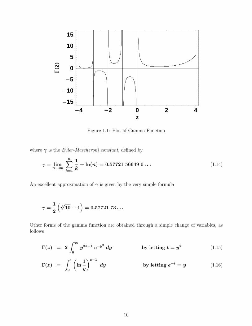
A plot of Γ(z) is shown in Figure 1.1.

Several other definitions of the Γ-function are available that can be attributed to the pio-neering mathematicians in this area

Gauss

Γ(z) = limn→∞

n! nz

z(z + 1)(z + 2) . . . (z + n), z �= 0, −1, −2, −3, . . . (1.12)

Weierstrass

1

Γ(z)= z eγ·z

∞∏n=1

(1 +

z

n

)e−z/n (1.13)

9

�4 �2 0 2 4z

�15

�10

�5

0

5

10

15

��z�

Figure 1.1: Plot of Gamma Function

where γ is the Euler-Mascheroni constant, defined by

γ = limn→∞

n∑k=1

1

k− ln(n) = 0.57721 56649 0 . . . (1.14)

An excellent approximation of γ is given by the very simple formula

γ =1

2

(3√

10 − 1)

= 0.57721 73 . . .

Other forms of the gamma function are obtained through a simple change of variables, asfollows

Γ(z) = 2

∫ ∞

0

y2z−1 e−y2

dy by letting t = y2 (1.15)

Γ(z) =

∫ 1

0

(ln

1

y

)z−1

dy by letting e−t = y (1.16)

10

Relations Satisfied by the Γ-Function

Recurrence Formula

Γ(z + 1) = z Γ(z) (1.17)

Duplication Formula

22z−1 Γ(z) Γ

(z +

1

2

)=

√π Γ(2z) (1.18)

Reflection Formula

Γ(z) Γ(1 − z) =π

sin πz(1.19)

Some Special Values of the Gamma Function

Using Eq. 1.15 or Eq. 1.19 we have

Γ(1/2) = (−1/2)! = 2

∫ ∞

0

e−y2

dy︸ ︷︷ ︸I

=√

π (1.20)

where the solution to I is obtained from Schaum’s Handbook of Mathematical Functions(Eq. 18.72).

11

Combining the results of Eq. 1.20 with the recurrence formula, we see

Γ(1/2) =√

π

Γ(3/2) =1

2Γ(1/2) =

√π

2

Γ(5/2) =3

2Γ(3/2) =

3

2

√π

2=

3√

π

4

...

Γ

(n +

1

2

)=

1 · 3 · 5 · · · (2n − 1)

2n

√π n = 1, 2, 3, . . .

For z > 0, Γ(z) has a single minimum within the range 1 ≤ z ≤ 2 at 1.46163 21450where Γ(z) = 0.88560 31944. Some selected 10 decimal place values of Γ(z) are found inTable 1.1.

Table 1.1: 10 Decimal Place Values of Γ(z) for 1 ≤ z ≤ 2

z Γ(z)

1.0 1.00000 000001.1 0.95135 076991.2 0.91816 874241.3 0.89747 069631.4 0.88726 381751.5 0.88622 692551.6 0.89351 534931.7 0.90863 873291.8 0.93138 377101.9 0.96176 583192.0 1.00000 00000

For other values of z (z �= 0, −1, −2. . . . ), Γ(z) can be computed by means of therecurrence formula.

12

Approximations

Asymptotic Representation of the Factorial and Gamma Functions

Asymptotic expansions of the factorial and gamma functions have been developed forz >> 1. The expansion for the factorial function is

z! = Γ(z + 1) =√

2πz zz e−z A(z) (1.21)

where

A(z) = 1 +1

12z+

1

288z2− 139

51840z3− 571

2488320z4+ · · · (1.22)

The expansion for the natural logarithm of the gamma function is

ln Γ(z) =

(z − 1

2

)ln z − z +

1

2ln(2π) +

1

12z− 1

360z3+

1

1260z5

− 1

1680z7+ · · · (1.23)

The absolute value of the error is less than the absolute value of the first term neglected.

For large values of z, i.e. as z → ∞, both expansions lead to Stirling’s Formula, given as

z! =√

2π zz+1/2 e−z (1.24)

Even though the asymptotic expansions in Eqs. 1.21 and 1.23 were developed for very largevalues of z, they give remarkably accurate values of z! and Γ(z) for small values of z. Table1.2 shows the relative error between the asymptotic expansion and known accurate valuesfor arguments between 1 ≤ z ≤ 7, where the relative error is defined as

relative error =approximate value − accurate value

accurate value

13

Table 1.2: Comparison of Approximate value of z! by Eq. 1.21 and Γ(z) by Eq. 1.23 withthe Accurate values of Mathematica 5.0

zz! Eq.1.21

z! Mathematicaerror

Γ(z) Eq.1.23

Γ(z) Mathematicaerror

1 0.99949 9469 −5.0 × 10−4 0.99969 2549 −3.1 × 10−4

2 0.99997 8981 −2.1 × 10−5 0.99999 8900 −1.1 × 10−6

3 0.99999 7005 −3.0 × 10−6 0.99999 9965 −3.5 × 10−8

4 0.99999 9267 −7.3 × 10−7 0.99999 9997 −2.8 × 10−9

5 0.99999 9756 −2.4 × 10−7 0.99999 9999 −4.0 × 10−10

6 0.99999 9901 −9.9 × 10−8 0.99999 9999 −7.9 × 10−11

7 0.99999 9954 −4.6 × 10−8 0.99999 9999 −2.0 × 10−11

The asymptotic expansion for Γ(z) converges very quickly to give accurate values for rela-tively small values of z. The asymptotic expansion for z! converges less quickly and doesnot yield 9 decimal place accuracy even when z = 7.

More accurate values of Γ(z) for small z can be obtained by means of the recurrence formula.For example, if we want Γ(1+z) where 0 ≤ z ≤ 1, then by means of the recurrence formulawe can write

Γ(1 + z) =Γ(n + z)

(1 + z)(2 + z)(3 + z) . . . (n − 1 + z)(1.25)

where n is an integer greater that 4. For n = 5 and z = 0.3, we have

Γ(1 + 0.3) =Γ(5.3)

(1.3)(2.3)(3.3)(4.3)= 0.89747 0699

This value can be compared with the 10 decimal place value given previously in Table 1.1.We observe that the absolute error is approximately 3 × 10−9. Comparable accuracy canbe obtained by means of the above equation with n = 6 and 0 ≤ z ≤ 1.

14

Polynomial Approximation of Γ(z + 1) within 0 ≤ z ≤ 1

Numerous polynomial approximations which are based upon the use of Chebyshev polyno-mials and the minimization of the maximum absolute error have been developed for varyingdegrees of accuracy. One such approximation developed for 0 ≤ z ≤ 1 due to Hastings8 is

Γ(z + 1) = z!

= 1 + z(a1 + z(a2 + z(a3 + z(a4 + z(a5 +

z(a6 + z(a7 + a8z))))))) + ε(z) (1.26)

where

|ε(z)| ≤ 3 × 10−7

and the coefficients in the polynomial are given as

Table 1.3: Coefficients of Polynomial of Eq. 1.26

a1 = −0.57719 1652 a5 = −0.75670 4078a2 = 0.98820 5891 a6 = 0.48219 9394a3 = −0.89705 6937 a7 = −0.19352 7818a4 = 0.91820 6857 a8 = 0.03586 8343

15

Series Expansion of 1/Γ(z) for |z| ≤ ∞

The function 1/Γ(z) is an entire function defined for all values of z. It can be expressed asa series expansion according to the relationship

1

Γ(z)=

∞∑k=1

Ckzk, |z| ≤ ∞ (1.27)

where the coefficients Ck for 0 ≤ k ≤ 26, accurate to 16 decimal places are tabulated inAbramowitz and Stegun1. For 10 decimal place accuracy one can write

1

Γ(z)=

19∑k=1

Ckzk (1.28)

where the coefficients are listed below

Table 1.4: Coefficients of Expansion of 1/Γ(z) of Eq. 1.28

k Ck k Ck

1 1.00000 00000 11 0.00012 805022 0.57721 56649 12 −0.00002 013483 −0.65587 80715 13 −0.00000 125044 −0.04200 26350 14 0.00000 113305 0.16653 86113 15 −0.00000 020566 −0.04219 77345 16 0.00000 000617 −0.00962 19715 17 0.00000 000508 0.00721 89432 18 −0.00000 000119 −0.00116 51675 19 0.00000 0000110 −0.00021 52416

16

Potential Applications

1. Gamma Distribution: The probability density function can be defined based on theGamma function as follows:

f(x, α, β) =1

Γ(α)βαxα−1e−x/β

This function is used to determine time based occurrences, such as:

• life length of an electronic component

• remaining life of a component

• waiting time between any two consecutive events

• waiting time to see the next event

• hypothesis tests

• confidence intervals

17

Digamma Function

The digamma function is the regularized (normalized) form of the logarithmic derivative ofthe gamma function and is sometimes referred to as the psi function.

ψ(z) =d ln Γ(z)

dz=

Γ′(z)

Γ(z)(1.29)

The digamma function is shown in Figure 1.2 for a range of arguments between −4 ≤ z ≤ 4.

�4 �2 0 2 4z

�20

�10

0

10

20

Ψ�z�

Figure 1.2: Plot of the Digamma Function

The ψ-function satisfies relationships which are obtained by taking the logarithmic derivativeof the recurrence, reflection and duplication formulas of the Γ-function. Thus

ψ(z + 1) =1

z+ ψ(z) (1.30)

ψ(1 − z) − ψ(z) = π cot(π z) (1.31)

ψ(z) + ψ(z + 1/2) + 2 ln 2 = 2ψ(2z) (1.32)

These formulas may be used to obtain the following special values of the ψ-function:

ψ(1) = Γ′(1) = −γ (1.33)

18

where γ is the Euler-Mascheroni constant defined in Eq. (1.14). Using Eq. (1.30)

ψ(n + 1) = −γ +n∑

k=1

1

kn = 1, 2, 3, . . . (1.34)

Substitution of z = 1/2 into Eq. (1.32) gives

ψ(1/2) = −γ − 2 ln 2 = −1.96351 00260 (1.35)

and with Eq. (1.30) we obtain

ψ(n + 1/2) = −γ − 2 ln 2 + 2n∑

k=1

1

2k − 1, n = 1, 2, 3, . . . (1.36)

Integral Representation of ψ(z)

The ψ-function has simple representations in the form of definite integrals involving thevariable z as a parameter. Some of these are listed below.

ψ(z) = −γ +

∫ 1

0

(1 − t)−1(1 − tz−1) dt, z > 0 (1.37)

ψ(z) = −γ − π cot(π z) +

∫ 1

0

(1 − t)−1(1 − t−z) dt, z < 1 (1.38)

ψ(z) =

∫ ∞

0

[e−t

t− e−zt

1 − e−t

]dt, z > 0 (1.39)

ψ(z) =

∫ ∞

0

[e−t − (1 + t)−z

] dt

t, z > 0

= −γ +

∫ ∞

0

[(1 + t)−1 − (1 + t)−z

] dt

t, z > 0 (1.40)

ψ(z) = ln z +

∫ ∞

0

[1

t− 1

1 − e−t

]e−zt dt, z > 0

= ln z − 1

2z−

∫ ∞

0

[1

1 − e−t− 1

t− 1

2

]e−zt dt, z > 0 (1.41)

19

Series Representation of ψ(z)

The ψ-function can be represented by means of several series

ψ(z) = −γ −∞∑

k=0

(1

z + k− 1

1 + k

)z �= −1, −2, −3, . . . (1.42)

ψ(x) = −γ − 1

x+ x

∞∑k=1

1

k(z + k)z �= −1, −2, −3, . . . (1.43)

ψ(z) = ln z −∞∑

k=0

[1

z + k− ln

(1 +

1

z + k

)]z �= −1, −2, −3, . . . (1.44)

Asymptotic Expansion of ψ(z) for Large z

The asymptotic expansion of the ψ-function developed for large z is

ψ(z) = ln z − 1

2z−

∞∑n=1

B2n

2nz2nz → ∞ (1.45)

where B2n are the Bernoulli numbers

B0 = 1 B6 = 1/42B2 = 1/6 B8 = −1/30B4 = −1/30 B10 = 5/66

(1.46)

The expansion can be expressed as

ψ(z) = ln z − 1

2z− 1

12z2+

1

120z4− 1

252z6+ · · · z → ∞ (1.47)

20

The Incomplete Gamma Function γ(z, x), Γ(z, x)

We can generalize the Euler definition of the gamma function by defining the incompletegamma function γ(z, x) and its compliment Γ(z, x) by the following variable limit integrals

γ(z, x) =

∫ x

0

e−t tz−1 dt z > 0 (1.48)

and

Γ(z, x) =

∫ ∞

x

e−t tz−1 dt z > 0 (1.49)

so that

γ(z, x) + Γ(z, x) = Γ(z) (1.50)

Figure 1.3 shows plots of γ(z, x), Γ(z, x) and Γ(z) all regularized with respect to Γ(z).We can clearly see that the addition of γ(z, x)/Γ(z) and Γ(z, x)/Γ(z) leads to a value ofunity or Γ(z)/Γ(z) for each value of z.

The choice of employing γ(z, x) or Γ(z, x) is simply a matter of analytical or computationalconvenience.

Some special values, integrals and series are listed below for convenience

Special Values of γ(z, x) and Γ(z, x) for “z” Integer (let z = n)

γ(1 + n, x) = n!

[1 − e−x

n∑k=0

xk

k!

]n = 0, 1, 2, . . . (1.51)

Γ(1 + n, x) = n! e−x

∞∑k=0

xk

k!n = 0, 1, 2, . . . (1.52)

Γ(−n, x) =(−1)n

n!

[Γ(0, x) − e−x

n−1∑k=0

(−1)kk!

xk+1

]n = 1, 2, 3 . . . (1.53)

21

0 2 4 6 8 10x

0.2

0.4

0.6

0.8

1

Γ�z

,x����z�

�z,x����z�, z � 1, 2, 3, 4 �

0 2 4 6 8 10x

0.2

0.4

0.6

0.8

1

��z

,x����z�

��z,x����z�, a � 1, 2, 3, 4 �

0 2 4 6 8 10x

0.2

0.4

0.6

0.8

1

��x����a�

��z����z�, a � 1, 2, 3, 4

Figure 1.3: Plot of the Incomplete Gamma Function whereγ(z, x)

Γ(z)+

Γ(z, x)

Γ(z)=

Γ(z)

Γ(z)

22

Integral Representations of the Incomplete Gamma Functions

γ(z, x) = xz cosec(π z)

∫ π

0

ex cos θ cos(zθ + x sin θ) dθ

x �= 0, z > 0, z �= 1, 2, . . . (1.54)

Γ(z, x) =e−xxz

Γ(1 − z)

∫ ∞

0

e−t t−z

x + tdt z < 1, x > 0 (1.55)

Γ(z, xy) = yze−xy

∫ ∞

0

e−ty (t + x)z−1 dt y > 0, x > 0, z > 1 (1.56)

Series Representations of the Incomplete Gamma Functions

γ(z, x) =∞∑

n=0

(−1)n xz+n

n! (z + n)(1.57)

Γ(z, x) = Γ(z) −∞∑

n=0

(−1)n xz+n

n! (z + n)(1.58)

Γ(z + x) = e−xxz

∞∑n=0

Lzn(x)

n + 1x > 0 (1.59)

where Lzn(x) is the associated Laguerre polynomial.

Functional Representations of the Incomplete Gamma Functions

γ(z + 1, x) = zγ(z, x) − xze−x (1.60)

Γ(z + 1, x) = zΓ(z, x) + xze−x (1.61)

Γ(z + n, x)

Γ(z + n)=

Γ(z, x)

Γ(z)+ e−x

n−1∑k=0

xz+k

Γ(z + k + 1)(1.62)

dγ(z, x)

dx= −dΓ(z, x)

dx= xz−1 e−x (1.63)

23

Asymptotic Expansion of Γ(z, x) for Large x

Γ(z, x) = xz−1 e−x

[1 +

(z − 1)

x+

(z − 1)(z − 2)

x2+ · · ·

]x → ∞ (1.64)

Continued Fraction Representation of Γ(z, x)

Γ(z, x) =e−x xz

z +1 − z

1 +1

x +2 − z

1 +2

x +3 − z

1 + . . .

(1.65)

for x > 0 and |z| < ∞.

Relationships with Other Special Functions

Γ(0, x) = −Ei(−x) (1.66)

Γ(0, ln 1/x) = −�i(x) (1.67)

Γ(1/2, x2) =√

π(1 − erf(x)) =√

π erfc(x) (1.68)

γ(1/2, x2) =√

π erf(x) (1.69)

γ(z, x) = z−1 xz e−x M(1, 1 + z, x) (1.70)

γ(z, x) = z−1 xz M(z, 1 + z, −x) (1.71)

24

Beta Function B(a, b)

Another definite integral which is related to the Γ-function is the Beta function B(a, b)which is defined as

B(a, b) =

∫ 1

0

ta−1 (1 − t)b−1 dt, a > 0, b > 0 (1.72)

The relationship between the B-function and the Γ-function can be demonstrated easily. Bymeans of the new variable

u =t

(1 − t)

Therefore Eq. 1.72 becomes

B(a, b) =

∫ ∞

0

ua−1

(1 + u)a+bdu a > 0, b > 0 (1.73)

Now it can be shown that

∫ ∞

0

e−pt tz−1 dt =Γ(z)

pz(1.74)

which is obtained from the definition of the Γ-function with the change of variable s = pt.Setting p = 1 + u and z = a + b, we get

1

(1 + u)a+b=

1

Γ(a + b)

∫ ∞

0

e−(1+u)t ta+b−1 dt (1.75)

and substituting this result into the Beta function in Eq. 1.73 gives

B(a, b) =1

Γ(a + b)

∫ ∞

0

e−t ta+b−1 dt

∫ ∞

0

e−ut ua−1 du

=Γ(a)

Γ(a + b)

∫ ∞

0

e−t tb−1 dt

=Γ(a) · Γ(b)

Γ(a + b)(1.76)

25

�4 �2 0 2 4y

�10

�5

0

5

10

15

B�y

,z�

Beta�y,.5�

Figure 1.4: Plot of Beta Function

All the properties of the Beta function can be derived from the relationships linking theΓ-function and the Beta function.

Other forms of the beta function are obtained by changes of variables. Thus

B(a, b) =

∫ ∞

0

ua−1 du

(1 + u)a+bby t =

u

1 − u(1.77)

B(a, b) = 2

∫ π/2

0

sin2a−1 θ cos2a−1 θ dθ by t = sin2 θ (1.78)

Potential Applications

1. Beta Distribution: The Beta distribution is the integrand of the Beta function. It canbe used to estimate the average time of completing selected tasks in time managementproblems.

Incomplete Beta Function Bx(a, b)

Just as one can define an incomplete gamma function, so can one define the incomplete betafunction by the variable limit integral

26

Bx(a, b) =

∫ x

0

ta−1 (1 − t)b−1 dt 0 ≤ x ≤ 1 (1.79)

with a > 0 and b > 0 if x �= 1. One can also define

Ix(a, b) =Bx(a, b)

B(a, b)(1.80)

Clearly when x = 1, Bx(a, b) becomes the complete beta function and

I1(a, b) = 1

The incomplete beta function and Ix(a, b) satisfies the following relationships:

Symmetry

Ix(a, b) = 1 − I1−x(b, a) (1.81)

Recurrence Formulas

Ix(a, b) = xIx(a − 1, b) + (1 − x)Ix(a, b − 1) (1.82)

(a + b − ax)Ix(a, b) = a(1 − x)Ix(a + 1, b − 1) + bIx(a, b + 1) (1.83)

(a + b)Ix(a, b) = aIx(a + 1, b) + bIx(a, b + 1) (1.84)

Relation to the Hypergeometric Function

Bx(a, b) = a−1xa F(a, 1 − b; a + 1; x) (1.85)

27

�4 �2 0 2 4y

�80

�60

�40

�20

0

20

40

B�x

,y,z�

Beta�.25, y, .5�

�4 �2 0 2 4y

�10

�5

0

5

10

B�x

,y,z�

Beta�.75, y, .5�

�4 �2 0 2 4y

�10

�5

0

5

10

15

B�x

,y,z�

Beta�1, y, .5�

Figure 1.5: Plot of the Incomplete Beta Function

28

Assigned Problems

Problem Set for Gamma and Beta Functions

1. Use the definition of the gamma function with a suitable change of variable to provethat

i)

∫ ∞

0

e−axxn dx =1

an+1Γ(n + 1) with n > −1, a > 0

ii)

∫ ∞

a

exp(2ax − x2) dx =

√π

2exp(a2)

2. Prove that

∫ π/2

0

sinn θ dθ =

∫ π/2

0

cosn θ dθ =

√π

2

Γ([1 + n]/2)

Γ([2 + n]/2)

3. Show that

Γ

(1

2+ x

)Γ

(1

2− x

)=

π

cos πx

Plot your results over the range −10 ≤ x ≤ 10.

4. Evaluate Γ

(−1

2

)and Γ

(−7

2

).

5. Show that the area enclosed by the axes x = 0, y = 0 and the curve x4 + y4 = 1 is

[Γ

(1

4

)]2

8√

π

Use both the Dirichlet integral and a conventional integration procedure to substantiatethis result.

29

6. Express each of the following integrals in terms of the gamma and beta functions andsimplify when possible.

i)

∫ 1

0

(1

x− 1

)1/4

dx

ii)

∫ b

a

(b − x)m−1(x − a)n−1 dx, with b > a, m > 0, n > 0

iii)

∫ ∞

0

dt

(1 + t)√

t

Note: Validate your results using various solution procedures where possible.

7. Compute to 5 decimal places

A

4ab=

1

2n

[Γ

(1

n

)]2

Γ

(2

n

)

for n = 0.2, 0.4, 0.8, 1.0, 2.0, 4.0, 8.0, 16.0, 32.0, 64.0, 100.0

8. Sketch x3 + y3 = 8. Derive expressions of the integrals and evaluate them in termsof Beta functions for the following quantities:

a) the first quadrant area bounded by the curve and two axesb) the centroid (x, y) of this areac) the volume generated when the area is revolved about the y−axisd) the moment of inertia of this volume about its axis

Note: Validate your results using various solution procedures where possible.

9. Starting with

Γ

(1

2

)=

∫ ∞

0

e−t dt√

t

and the transformation y2 = t or x2 = t, show that

30

[Γ

(1

2

)]2

= 4

∫ ∞

0

∫ ∞

0

exp[−(x2 + y2)

]dx dy

Further prove that the above double integral over the first quadrant when evaluatedusing polar coordinates (r, θ) yields

Γ

(1

2

)=

√π

31

References1. Abramowitz, M. and Stegun, I.A., (Eds.), “Gamma (Factorial) Function” and

“Incomplete Gamma Function.” §6.1 and §6.5 in Handbook of Mathematical Functionsand Formulas, Graphs and Mathematical Tables, 9th printing, Dover, New York, 1972,pp. 255-258 and pp 260-263.

2. Andrews, G.E., Askey, R. and Roy, R., Special Functions, Cambridge UniversityPress, Cambridge, 1999.

3. Artin, E. The Gamma Function, Holt, Rinehart, and Winston, New York, 1964.

4. Barnew, E.W., “The Theory of the Gamma Function,” Messenger Math., (2), Vol.29, 1900, pp.64-128..

5. Borwein, J.M. and Zucker, I.J., “Elliptic Integral Evaluation of the Gamma Func-tion at Rational Values and Small Denominator,” IMA J. Numerical Analysis, Vol.12, 1992, pp. 519-526.

6. Davis, P.J., “Leonhard Euler’s Integral: Historical profile of the Gamma Function,”Amer. Math. Monthly, Vol. 66, 1959, pp. 849-869.

7. Erdelyl, A., Magnus, W., Oberhettinger, F. and Tricomi, F.G., “The GammaFunction,” Ch. 1 in Higher Transcendental Functions, Vol. 1, Krieger, New York,1981, pp. 1-55.

8. Hastings, C., Approximations for Digital Computers, Princeton University Press,Princeton, NJ, 1955.

9. Hochstadt, H., Special Functions of Mathematical Physics, Holt, Rinehart and Win-ston, New York, 1961.

10. Koepf, W.. “The Gamma Function,” Ch. 1 in Hypergeometric Summation: AnAlgorithmic Approach to Summation and Special Identities, Vieweg, Braunschweig,Germany, 1998, pp. 4-10.

11. Krantz, S.C., “The Gamma and Beta Functions,” §13.1 in Handbook of ComplexAnalysis, Birkhauser, Boston, MA, 1999, pp. 155-158.

12. Legendre, A.M., Memoires de la classe des sciences mathematiques et physiques del’Institut de France, Paris, 1809, p. 477, 485, 490.

13. Magnus, W. and Oberhettinger, F., Formulas and Theorems for the Special Func-tions of Mathematical Physics, Chelsea, New York, 1949.

14. Saibagki, W., Theory and Applications of the Gamma Function, Iwanami Syoten,Tokyo, Japan, 1952.

15. Spanier, J. and Oldham, K.B., “The Gamma Function Γ(x)” and “The IncompleteGamma γ(ν, x) and Related Functions,” Chs. 43 and 45 in An Atlas of Functions,Hemisphere, Washington, DC, 1987, pp. 411-421 and pp. 435-443.

32