FEDERAL RESERVE BANK OF SAN FRANCISCO

WORKING PAPER SERIES

Factor Specificity and Real Rigidities

Carlos Carvalho PUC-Rio

Fernanda Nechio

Federal Reserve Bank of San Francisco

August 2016

Carvalho, Carlos, Fernanda Nechio. 2016. “Factor Specificity and Real Rigidities.” Federal Reserve Bank of San Francisco Working Paper 2013-31. http://www.frbsf.org/economic-research/publications/working-papers/wp2013-31.pdf The views in this paper are solely the responsibility of the authors and should not be interpreted as reflecting the views of the Federal Reserve Bank of San Francisco or the Board of Governors of the Federal Reserve System.

Working Paper 2013-31 http://www.frbsf.org/economic-research/publications/working-papers/wp2013-31.pdf

Factor Specificity and Real Rigidities∗

Carlos Carvalho

Central Bank of Brazil and PUC-Rio

Fernanda Nechio

Federal Reserve Bank of San Francisco

August, 2016

Abstract

We develop a multisector model in which capital and labor are free to move across

firms within each sector, but cannot move across sectors. To isolate the role of sec-

toral specificity, we compare our model with otherwise identical multisector economies

with either economy-wide or firm-specific factor markets. Sectoral factor specificity gen-

erates within-sector strategic substitutability and tends to induce across-sector strategic

complementarity in price setting. Our model can produce either more or less monetary

non-neutrality than those other two models, depending on parameterization and the dis-

tribution of price rigidity across sectors. Under the empirical distribution for the U.S.,

our model behaves similarly to an economy with firm-specific factors in the short-run, and

later on approaches the dynamics of the model with economy-wide factor markets. This

is consistent with the idea that factor price equalization might take place gradually over

time, so that firm-specificity may serve as a reasonable short-run approximation, whereas

economy-wide markets are likely a better description of how factors of production are

allocated in the longer run.

JEL classification codes: E22, J6, E12

Keywords: factor specificity, multisector model, heterogeneity, monetary non-neutrality

∗For comments and suggestions we thank seminar participants at ESEM 2014, SED 2014, NASM 2014.The views expressed in this paper are those of the authors and do not necessarily reflect the position of theFederal Reserve Bank of San Francisco, the Federal Reserve System or the Central Bank of Brazil. E-mails:cvianac@econ.puc-rio.br, fernanda.nechio@sf.frb.org. Corresponding author: fernanda.nechio@sf.frb.org.

1

1 Introduction

Much of the monetary economics literature tries to make sense of the extent of monetary non-

neutrality that is apparent in the data. An important part of this literature does so by resorting

to models in which prices (and sometimes wages) are sticky. A problem with bare bone versions

of these models is that the degree of price rigidity required to generate substantial non-neutrality

is at odds with the microeconomic evidence on the frequency of price changes. However, since

Ball and Romer (1990) and Kimball (1995), it is well-known that large real rigidities – which

can induce strategic complementarities in price-setting decisions – can generate substantial

endogenous persistence in the real effects of monetary shocks, and thus help bridge this gap.

In a series of contributions to our understanding of the sources of real rigidities, Woodford

(2003, chap.3), Sveen and Weinke (2005), and Woodford (2005) argue forcefully that factor

specificity matters. Woodford (2003, chap.3) focuses on firm-specific labor,1 whereas Sveen and

Weinke (2005) develop a model with firm-specific capital.2 In turn, Woodford (2005) studies a

model in which both capital and labor are specific to firms. He shows that capital and labor

specificity at the firm level are a powerful source of real rigidities.

The assumption of firm-level specificity contrasts sharply with the (usually unstated) as-

sumption that factors of production can move freely across firms, as in the Real Business Cycle

literature. Under standard assumptions about preferences and technology, such economy-wide

factor markets tend to induce strategic substitutability in price setting (e.g., Woodford, 2005,

chap.3), and thus generate a small degree of monetary non-neutrality (Chari, Kehoe and Mc-

grattan, 2000).

The two aforementioned assumptions about factor markets are, to some extent, unrealistic.

It is likely that factor price equalization takes place gradually over time, so that firm-specificity

might be a reasonable short-run approximation, whereas economy-wide markets might be a

better description of how factors of production are allocated in the longer run.

In this paper, we study whether the nature of factor specificity matters. To that end, we

develop a multisector model in which both capital and labor are free to move across firms within

each sector, but cannot move across sectors – i.e., factors of production are sector-specific. To

isolate the role of sectoral specificity, we compare our model with otherwise identical multisector

economies with either economy-wide or firm-specific factor markets.

1To be precise, Woodford (2003, 2005)’s models feature industry-specific labor coupled with assumptionsthat make it mathematically equivalent to a particular model with firm-specific labor markets, as will becomeclear subsequently.

2Other papers in the literature, such as Sveen and Weinke (2007a,b) and Altig et al. (2011), also find thatfirm-specific capital is an important ingredient for understanding the monetary transmission mechanism. Reiter,Sveen and Weinke (2013) analyze the role of capital specificity in a model with lumpy (S,s) investment.

2

It turns out that it matters a great deal whether factor markets are specific at the firm

or at the sector level. Using simplified versions of the three models, we illustrate analytically

how the degree of strategic complementarity or substitutability in pricing decisions differ across

the three models. As a result of different patterns of pricing interactions within and across

sectors, our model with sector-specific factor markets can produce rich aggregate dynamics.

Sectoral factor specificity generates within-sector strategic substitutability in pricing decisions.

This tends to reduce the degree of monetary non-neutrality relative to the case of firm-specific

factors. At the same time, sectoral relative price movements generate distributional effects that

induce strategic complementarity (or weaken strategic substitutability) in pricing decisions

across sectors – relative to the model with economy-wide factor markets. As a result of these

forces, our sector-specific factor model can produce either more or less monetary non-neutrality

than those other two models, depending on parameterization and the distribution of price

rigidity across sectors.

Turning back to the fully-specified versions of the three models, our results show that a

calibrated version of our model that matches the empirical distribution of price stickiness for

the U.S. behaves similarly to an economy with firm-specific factors in the short-run, and later

on approaches the dynamics of the model with economy-wide factor markets.

The differences in aggregate dynamics implied by the different assumptions on factor speci-

ficity can also be understood through the lens of the underlying New Keynesian Phillips curves.

We explicitly derive Phillips curves in our multisector economies with endogenous capital ac-

cumulation, under the three alternative assumptions regarding factor specificity.3

While the assumption that factors cannot move across sectors is also extreme, our model

is motivated by existing empirical evidence that both capital and labor have an important

degree of sector (or industry) specificity. For example, Ramey and Shapiro (1998) find that the

flow of capital across firms within the same industry is indeed large, while Ramey and Shapiro

(2001) provide evidence of significant sectoral specificity of capital, based on an industry case

study. Davis and Haltiwanger (1992) and Parent (2000) provide empirical evidence that labor

reallocation across sectors/industries is more limited than within sectors. More recently, Hobijn

(2012) finds similar results. Autor et al. (2014) show that the intensity of labor reallocation

within- versus across- sectors correlates with the level of wages. In particular, looking at the

effects of increasing import competition, they find that low-wage workers reallocate primarily

within industry, while high-wage workers appear to switch sectors more easily. Dix-Carneiro

(2014) estimates the effects of a trade liberalization shock in Brazil using a model with imperfect

3For an analysis of the implications of labor specificity for the New Keynesian Phillips Curve (NKPC) inone-sector models without capital accumulation, see the recent survey by Leahy (2011).

3

labor and capital mobility across sectors. He finds that these mobility frictions lead to a slower

response of the economy to shocks.

Different forms of input specificity can also be justified on theoretical grounds. In a series

of contributions, Caballero (2007), and Caballero and Hammour (1996, 1998, 2000) discuss the

possible sources and macroeconomic implications of input specificity. They show that speci-

ficity contributes to the slow adjustment of macroeconomic aggregates to shocks in the short

and medium run, with resources being underutilized, production suffering from “technological

sclerosis,” and recessions being excessively sharp in the transition to a new steady state.

Section 2 presents the reference model of our multisector economy with sector-specific factors

of production. It also presents the otherwise identical multisector models with either economy-

wide or firm-specific factor markets. Section 3 analyses in detail the different patterns of pricing

interactions produced by the three models, and presents the underlying new Keynesian Phillips

curves. Section 4 follows with a quantitative analysis of the effects of monetary shocks under

the three types of factor specificity. The last section concludes.

2 Three models of factor specificity

In this section, we consider three alternative sticky-price dynamic stochastic general equilibrium

(DSGE) models that differ in their assumptions about factor mobility. In all models, identical

infinitely-lived consumers supply labor and capital to intermediate firms that they own, invest

in a complete set of state-contingent financial claims, and consume a final good. The latter is

produced by competitive firms that bundle varieties of intermediate goods. The monopolisti-

cally competitive intermediate firms that produce these varieties are divided into sectors that

differ in their frequency of price changes. Labor and capital are the only variable inputs in the

production of intermediate goods. In the first model, presented in Section 2.1, we assume that

these inputs can be reallocated freely across firms in the same sector but cannot flow across

sectors, i.e., factors are sector-specific.4 Sections 2.2 and 2.3 consider two alternative cases in

which factors of production are, respectively, firm-specific or can move freely across firms and

sectors (“economy-wide” factor markets).

4Woodford sometimes refers to his assumption regarding labor markets as involving industry-specific (e.g.,Woodford, 2003, chap.3) or sector-specific (e.g., Woodford, 2005) labor markets. This is not the same asour assumption of sector-specificity. In Woodford’s work, an industry (or sector) is characterized by fullysynchronized price setting, so that his assumption is mathematically equivalent to firm-specific labor markets– as long as firms do not try to exploit their monopsony power and take wages as given. In contrast, in ourmodel, price changes are asynchronized within each sector.

4

2.1 Sector-specific factors

The representative consumer maximizes:

E0

∞∑t=0

βt

(C1−σt − 1

1− σ−

S∑s=1

ωsN1+γs,t

1 + γ

),

subject to the flow budget constraint:

PtCt + PtIt + Et [Θt,t+1Bt+1] ≤S∑s=1

Ws,tNs,t +Bt + Tt +S∑s=1

Zs,tKs,t,

the law of motion for the stocks of sector-specific capital:

Ks,t+1 = (1− δ)Ks,t + Φ (Is,t, Ks,t) Is,t, ∀ s

Is,t ≥ 0,∀s,

and a standard “no-Ponzi” condition. Et denotes the time-t expectations operator, Ct is con-

sumption of the final good, Ns,t denotes total labor supplied to firms in sector s, Ws,t is the

associated nominal wage rate, and ωs is the relative disutility of supplying labor to sector s.5

Is,t denotes investment in sector-s capital, It ≡∑S

s=1 Is,t, Ks,t is capital supplied to firms in

sector s, and Zs,t is the associated nominal return on capital. The final good can be used for

either investment or consumption, and sells at the nominal price Pt. Bt+1 accounts for the

state-contingent value of the portfolio of financial securities held by the consumer at the begin-

ning of t + 1. Under complete financial markets, agents can choose the value of Bt+1 for each

possible state of the world at all times, subject to the no-Ponzi condition and the budget con-

straint. Tt stands for profits received from intermediate firms. The absence of arbitrage implies

the existence of a nominal stochastic discount factor Θt,t+1 that prices in period t any financial

asset portfolio with state-contingent payoff Bt+1 at the beginning of period t + 1.6 Finally, β

is the time-discount factor, σ−1 denotes the intertemporal elasticity of substitution, γ−1 is the

Frisch elasticity of labor supply,7 δ is the rate of depreciation, and Φ (.) is the adjustment-cost

5As in Carvalho and Lee (2011), the relative labor disutility parameter ωs is only used to obtain a symmetricsteady state, and simplify the algebra. It does not play a role in any of our findings. Derivation details areavailable upon request.

6To avoid cluttering the notation, we omit explicit reference to the different states of nature.7Our approach to modeling labor specificity follows Woodford (2003) and hinges on introducing the convexity

of labor disutility at the level at which the specificity exists. This creates the possibility of wage dispersionarising at that level. Hence, in our model with sectoral factor markets, labor disutility is given by the sum ofconvex functions of sectoral labor supplies. Likewise, in the model with firm-specific labor (Section 2.2), suchconvexity applies to the amount of labor supplied to each firm. If convexity kicks in at the level of total labor

5

function.8 We follow Chari, Kehoe and Mcgrattan (2000) and assume:

Φ (Is,t, Ks,t) = Φ

(Is,tKs,t

)= 1− 1

2κ

(Is,tKs,t− δ)2

Is,tKs,t

,

which is convex and satisfies Φ (δ) = 1, Φ′ (δ) = 0, and Φ′′ (δ) = −κδ. For brevity, we present

the (standard) optimality conditions in the online Appendix.

A representative competitive firm produces the final good, which is a composite of varieties

of intermediate goods. Monopolistically competitive firms produce such varieties. The latter

firms are divided into sectors indexed by s ∈ {1, ..., S}, each featuring a continuum of firms.

Sectors differ in the degree of price rigidity, as we detail below. Overall, firms are indexed by

their sector s, and are further indexed by j ∈ [0, 1]. The distribution of firms across sectors is

given by sectoral weights fs > 0, with∑S

s=1 fs = 1.

The final good is used for both consumption and investment and is produced by combining

the intermediate varieties according to the technology:

Yt =

(∑S

s=1f

1ηs Y

η−1η

s,t

) ηη−1

, (1)

Ys,t =

(fθ−1θ

s

∫ 1

0

Yθ−1θ

s,j,t dj

) θθ−1

, (2)

where Yt is the final good, Ys,t is the aggregation of sector-s intermediate goods, and Ys,j,t is

the variety produced by firm j in sector s. The parameters η ≥ 0, and θ > 1 are, respectively,

the elasticity of substitution across sectors, and the elasticity of substitution within sectors.

The representative final-good-producing firm solves:

max PtYt −∑S

s=1fs

∫ 1

0

Ps,j,tYs,j,tdj

s.t. (1)-(2),

supply, wages are equalized – and this is what characterizes our model with an economy-wide labor market(Section 2.3).

8In the absence of (convex) adjustment costs, returns to capital (and Tobin’s qs) are equalized across sectors.Hence, our approach to modeling capital specificity hinges on introducing adjustment costs in the ”right place”,so as to allow for dispersion in returns to capital (across sectors in the sector-specific model, and across firmsin the firm-specific model of Section 2.2).

6

which yields as first-order conditions, for j ∈ [0, 1] and s = 1, ..., S:

Ys,j,t =

(Ps,j,tPs,t

)−θ (Ps,tPt

)−ηYt.

The price indices are given by:

Pt =(∑S

s=1fsP

1−ηs,t

) 11−η

,

Ps,t =

(∫ 1

0

P 1−θs,j,t dj

) 11−θ

,

where Pt is the price of the final good, Ps,t is the price index of sector-s intermediate goods,

and Ps,j,t is the price charged by firm j from sector s.

Monopolistically competitive firms produce varieties of the intermediate good by employing

capital and labor. For analytical tractability, we assume that intermediate firms set prices as in

Calvo (1983). The frequency of price changes varies across sectors, and it is the only source of

(ex-ante) heterogeneity. While in reality sectors certainly differ in many dimensions other than

heterogeneity in price stickiness, this assumption suits our purposes for the following reasons.

First, nominal rigidity is of interest, because our goal is to contribute to the literature on factor

specificity as a source of real rigidities that can amplify/propagate monetary shocks (e.g., Chari,

Kehoe and Mcgrattan, 2000 and Woodford, 2005). In this context, allowing for heterogeneity in

price stickiness is natural, because of the ample literature documenting that this is empirically

important, and that it matters for aggregate dynamics.9 In addition, in our model, any two

different sectors that have the same degree of price rigidity will respond to aggregate shocks

in the exact same way.10 Hence, our partition of the economy in terms of price rigidity may

encompass arbitrarily many “subsectors” within each sector.

In each period, each firm j in sector s changes its price independently with probability αs.

At each time a firm j from sector s adjusts its price, it chooses Xs,j,t to solve:

max Et

∞∑l=0

Θt,t+l (1− αs)l[Xs,j,tYs,j,t+l −Ws,t+lNs,j,t+l − Zs,t+lKs,j,t+l

]s.t. Ys,j,t =

(Ps,j,tPs,t

)−θ (Ps,tPt

)−ηYt (3)

Ys,j,t = (Ks,j,t)1−χ (Ns,j,t)

χ , (4)

9See, for example, the survey by Klenow and Malin (2011).10This would possibly cease to be the case if sectors differed in other dimensions as well.

7

where χ is the elasticity of output with respect to labor.

Optimal price setting implies:

Xs,j,t =θ

θ − 1

Et∑∞

l=0 Θt,t+l (1− αs)l Λs,t+l

(χK1−χ

s,j,t+lNχ−1s,j,t+l

)−1Ws,t+l

Et∑∞

l=0 Θt,t+l (1− αs)l Λs,t+l

,

where:

Λs,t =

(1

Ps,t

)−θ (Ps,tPt

)−ηYt.

From cost-minimization, real marginal cost can be expressed as:

MCs,j,t = MCs,t =1

χχ (1− χ)1−χ

(Ws,t

Pt

)χ(Zs,tPt

)(1−χ)

.

Note that marginal costs are equalized only within sectors. This is a direct implication of

the assumption of sectoral capital and labor markets. Finally, under that assumption, the

market-clearing conditions for capital and labor are:

Ks,t = fs

∫ 1

0

Ks,j,tdj, ∀ s,

Ns,t = fs

∫ 1

0

Ns,j,tdj, ∀ s.

2.2 Firm-specific factors

We now consider a variant of the previous model in which production inputs are firm-specific.

This version of the model generalizes Woodford (2005) to a multisector economy. It requires that

we reformulate the consumers’ and intermediate firms’ problems. The maximization problem

of final goods firms remains the same as in the model with sectoral factor markets.

The representative consumer maximizes:

E0

∞∑t=0

βt

(C1−σt − 1

1− σ−

S∑s=1

fs

∫ 1

0

N1+γs,j,t

1 + γdj

),

subject to the flow budget constraint:

PtCt + PtIt + Et [Θt,t+1Bt+1] ≤S∑s=1

fs

∫ 1

0

Ws,j,tNs,j,tdj +Bt + Tt +S∑s=1

fs

∫ 1

0

Zs,j,tKs,j,tdj,

8

the law of motion for the stocks of firm-specific capital:

Ks,j,t+1 = (1− δ)Ks,j,t + Φ (Is,j,t, Ks,j,t) Is,j,t,∀ s, j

Is,j,t ≥ 0,∀ s, j,

where Φ (Is,j,t, Ks,j,t) now takes the form:

Φ (Is,j,t, Ks,j,t) = Φ

(Is,j,tKs,j,t

)= 1− 1

2κ

(Is,j,tKs,j,t

− δ)2

Is,j,tKs,j,t

,

and a standard “no-Ponzi” condition.

The notation is the same as before, except that now Ns,j,t denotes total labor supplied to

firm j in sector s, and Ws,j,t is the associated nominal wage rate. Is,j,t denotes investment

allocated to firm j in sector s, It ≡∑S

s=1 fs∫ 1

0Is,j,tdj, Ks,j,t is capital supplied to firm j in

sector s, and Zs,j,t is the associated nominal return on capital.

Once we introduce firm-specific factor markets, the intermediate goods producer’s problem

also changes since wages and the return on capital will also be firm-specific:

max Et

∞∑l=0

Θt,t+l (1− αs)l[

Xs,j,tYs,j,t+l+

−Ws,j,t+lNs,j,t+l − Zs,j,t+lKs,j,t+l

]s.t. (3) and (4).

The solutions to the consumer and the intermediate firms problems yield first-order condi-

tions that are similar to those obtained for the sector-specific model except that the resulting

choices of labor, Ns,j,t, investment, Is,j,t, and capital Ks,j,t are firm-specific. This implies that

the return on labor and capital (Ws,j,t and Zs,j,t, respectively) and real marginal costs are also

firm-specific. Optimality conditions are presented in the online Appendix.

2.3 Economy-wide factor markets

Finally, we consider a version of the model in which labor and capital can move freely across

firms and sectors. This requires that we reformulate the consumers’ and intermediate firms’

problems once again. The maximization problem of final goods’ firms remains the same as

before.

9

The representative consumer maximizes:

E0

∞∑t=0

βt(C1−σt − 1

1− σ− N1+γ

t

1 + γ

),

subject to the flow budget constraint:

PtCt + PtIt + Et [Θt,t+1Bt+1] ≤ WtNt +Bt + Tt + ZtKt,

the law of motion for capital stocks:

Kt+1 = (1− δ)Kt + Φ (It, Kt) It,

It ≥ 0,

where Φ (It, Kt) now takes the form:

Φ (It, Kt) = Φ

(ItKt

)= 1− 1

2κ

(ItKt− δ)2

ItKt

,

and a standard “no-Ponzi” condition.

The notation is the same as before, except that Nt is total labor supply, Wt is the corre-

sponding nominal wage rate, It denotes investment, Kt stands for capital, Zt is the associated

nominal return on capital.

Under economy-wide capital and labor markets, the intermediate firm’s problem becomes:

max Et

∞∑l=0

Θt,t+l (1− αs)l[

Xs,j,tYs,j,t+l+

−Wt+lNs,j,t+l − Zt+lKs,j,t+l

]s.t. (3) and (4).

The first-order conditions for the economy-wide model yield returns to labor and capital

(Wt and Zt, respectively), and hence, real marginal costs (MCt) that equalize across all firms

and sectors. For optimality conditions, see online Appendix.

2.4 Monetary policy

In our baseline specification we assume that the growth rate of nominal aggregate demand

follows a first-order autoregressive, AR(1), process, thus leaving monetary policy implicit. This

is a common assumption in the literature (e.g. Mankiw and Reis, 2002). Denoting nominal

10

aggregate demand by Mt ≡ PtYt, we assume:

∆mt = ρm∆mt−1 + σεmεm,t,

where mt ≡ log (Mt), ρm determines the autocorrelation in nominal aggregate demand growth,

and εm,t is a purely monetary, uncorrelated, zero-mean, unit-variance i.i.d. shock.

We analyze the model using a loglinear approximation around the zero-inflation steady state.

While solving the models with sectoral and economy-wide factor markets is straightforward, the

model with firm-specific capital is more challenging. The reason is that firms can have different

capital-accumulation histories. We solve that model by generalizing the approach pioneered by

Woodford (2005) to the case of a multisector economy. Details of the solution are available in

the online Appendix.

3 The underlying New Keynesian Phillips curves

Each model of Section 2 gives rise to a distinct New Keynesian Phillips curve (NKPC), with

different implications for aggregate dynamics.11 As a first step to understand those differences,

we can develop some intuition by analyzing the so-called frictionless optimal prices in each

model – i.e., the prices that firms would set if they could change them continuously.

For simplicity, we work with versions of the model without capital (χ = 1).12 In that case,

the expressions for the frictionless optimal prices in the economy-wide, sector- and firm-specific

economies are given by, respectively:

Economy-wide: p∗s,j,t = (σ + γ)mt + (1− σ − γ) pt (5)

Sector-specific: p∗s,j,t = (σ + γ)mt + (1− σ − γ + ηγ) pt − ηγps,t (6)

Firm-specific: p∗s,j,t =σ + γ

1 + θγmt +

1− σ − γ + ηγ

1 + θγpt +

(θ − η) γ

1 + θγps,t, (7)

where p∗s,j,t is the frictionless optimal price of firm j in sector s.

The coefficients associated with the aggregate price level (pt) and with sectoral prices (ps,t)

indicate how a firm would like to respond to changes in those prices. That is, they determine the

nature of pricing interactions in the three economies. Note that, because these are multisector

economies, it is possible that firms’ pricing decisions interact differently, depending on whether

firms are in the same sector or in different sectors. We refer to the dependence of p∗s,j,t on ps,t

11Derivations are available upon request.12Hence, the analysis in this section is similar to that in Carvalho and Lee (2011).

11

as resulting from within-sector pricing interactions, and to the effect of pt on p∗s,j,t as resulting

from across-sector pricing interactions.13

A positive coefficient on the aggregate price level, say, implies that a firm’s frictionless

optimal price rises when other prices increase. That is, such a positive coefficient implies

a strategic complementarity with respect to the overall level of prices in the economy (i.e.,

across-sector complementarity). Likewise, a negative coefficient on the sectoral price index

implies strategic substitutability with respect to the prices of firms in the same sector (i.e.,

within-sector substitutability).

In order to think through the patterns of pricing interactions that the three models can

deliver, let us start with the case of economy-wide factor markets (equation 5). In that model,

in response to, say, an increase in the aggregate price level, a firm j in sector s will have an

incentive to increase, decrease, or to keep its price unchanged depending on whether (1− σ − γ)

is positive, negative, or zero, respectively. So, to fix ideas, let us consider as a benchmark the

parameterization under which the economy-wide model features strategic neutrality in price

setting – i.e., when σ + γ = 1. We can, then, more easily compare the three models.

When σ+γ = 1, both the sector- and the firm-specific models tend to induce strategic com-

plementarity in price setting across sectors. This happens as long as ηγ > 0 – that is, as long as

there is some substitution between varieties in different sectors (η > 0) and the Frisch elasticity

of labor supply is finite (γ > 0). Note also, that, as long as the latter condition holds (γ > 0),

the degree of across-sector pricing complementarities in the model with sector-specific labor is

larger than in the model with firm-specific labor: 1− σ− γ+ ηγ ≥ (1− σ − γ + ηγ) / (1 + θγ).

The two models of labor specificity, however, differ markedly in their implications for the

pattern of pricing interactions within sectors (assuming ηγ > 0). While the model with sector-

specific labor necessarily induces strategic substitutability within sectors, the firm-specific

model features within-sector strategic complementarity as long as the elasticity of substitu-

tion between varieties within any given sector exceeds the elasticity of substitution between

varieties across sectors (θ > η) – which seems plausible.

When σ + γ 6= 1, the pattern of pricing interactions can differ even more across the three

economies, depending on parameter values. Let us now turn to the economic mechanisms

underlying these possible patterns of pricing interactions. We rely on the usual thought exper-

iment of considering exogenous changes in aggregate or sectoral prices, while keeping nominal

aggregate demand constant.

We start with the economy-wide factors model. In this model, it is clear from equation

13Strictly speaking, this separation of the effects of ps,t and pt on p∗s,j,t only holds exactly if sectors havenegligible mass. Nevertheless, we adopt this terminology for expositional convenience.

12

(5) that sectoral prices have no effect on a firm’s frictionless optimal price. The reason is

that, in the labor-only models that we entertain in this section, that price is proportional to

the nominal wage. With an economy-wide labor market, the nominal wage only depends on

the aggregate price level, aggregate labor, and aggregate consumption. These are unaffected

by changes in sectoral prices that keep the aggregate price level constant (which is the right

thought experiment to isolate how sectoral prices affect a firm’s frictionless optimal price).

Turning to the effects of the aggregate price level on a firm’s frictionless optimal price, let us

consider an exogenous increase in the overall level of prices. With nominal aggregate demand

constant by assumption, consumption falls (in the proportion of the price increase) – and so

does labor. Whether the nominal wage ends up increasing, decreasing, or unchanged thus hinges

on the Frisch elasticity of labor supply and on the intertemporal elasticity of substitution in

consumption.14 If these elasticities are large (i.e., γ and σ are small), the real wage falls

relatively little. That is, the nominal wage – and hence, a firm’s frictionless optimal price –

moves closely with the aggregate price level. This explains why pricing decisions are strategic

complements when the Frisch elasticity of labor supply and/or the intertemporal elasticity of

substitution in consumption are large enough (so that γ + σ < 1). The knife-edge case of

strategic neutrality (γ + σ = 1) arises precisely when these elasticities are such that the drop

in consumption and labor exactly offset the aggregate price increase and keep nominal wages

unchanged.

We now take up the case of firm-specific labor. Once again, understanding the effects of

changes in aggregate or sectoral prices on a firm’s frictionless optimal price requires understand-

ing their effects on nominal wages. The difference is that, now, wages depend on aggregate con-

sumption and firm-level, as opposed to aggregate, employment. As before, let us first consider

an exogenous increase in the overall level of prices. With nominal aggregate demand constant

by assumption, consumption falls like before (in the proportion of the price increase). But, in

general, the level of labor employed by the firm under consideration can increase or decrease.

On the one hand, the drop in aggregate demand tends to lower that firm’s demand for labor,

just as in the economy-wide case. On the other hand, the assumed aggregate price increase

makes the firm’s variety relatively cheaper. This increases demand for its variety, and hence its

demand for labor. For parameter values that imply strategic neutrality in the economy-wide

model (γ + σ = 1), we can conclude that the nominal wage ends up increasing. The reason

is that, for those parameter values, the drop in aggregate consumption and its negative effect

on the firm’s labor demand exactly offset the aggregate price increase. So, the net effect on

14In the model with economy-wide factors, this can be easily seen from the optimality condition for labor:Wt

Pt= Nγ

t Cσt . For details, see the online Appendix.

13

the nominal wage the firm has to pay its workers is positive, and is dictated by the increase in

relative demand for its variety.15

Continuing with the model with firm-specific labor, let us now analyze the effects of a

change in the level of prices in a given sector (ps,t) on the frictionless optimal price of a firm

in that sector (p∗s,j,t). For concreteness, let us assume an increase in ps,t. What matters for

the effect of such a price change on the nominal wage that firm j has to pay its worker is

whether the firm ends up having to employ more or less labor. There are two opposite forces

at work. First, the increase in ps,t reduces the demand for varieties of all firms in sector s.

This effect is dictated by the elasticity of substitution between varieties across sectors (η).

The second effects arises because the assumed sectoral price increase makes firm j’s variety

relatively cheaper. This increases demand for its variety, and hence its demand for labor.

This effect is dictated by the elasticity of substitution between varieties in the same sector (θ).

Under the plausible assumption that the elasticity of substitution between varieties within any

given sector exceeds the elasticity of substitution between varieties across sectors (θ > η), the

net effect on firm j’s employment, and hence on the nominal wage it has to pay its workers,

is positive. Therefore, under this assumption, the firm-specific model features across-sector

strategic complementarities in price-setting decisions.

We now turn to the model with sector-specific labor markets. Like before, understanding the

effects of changes in aggregate or sectoral prices on a firm’s frictionless optimal price requires

understanding their effects on nominal wages. The difference is that, now, wages depend on

aggregate consumption and employment at the sector – as opposed to aggregate or firm – level.

Consider first an exogenous increase in the overall level of prices. With nominal aggregate

demand constant by assumption, consumption falls like before (in the proportion of the price

increase). But, in general, the level of labor employed in the sector under consideration can

increase or decrease. On the one hand, the drop in aggregate demand tends to lower the sector’s

demand for labor. On the other hand, the assumed aggregate price increase makes all varieties

in that sector relatively cheaper. This increases demand for that sector’s output, and hence its

demand for labor. For parameter values that imply strategic neutrality in the economy-wide

model (γ+σ = 1), we can conclude that the nominal wage in the sector at hand increases. The

reason is that, for those parameter values, the drop in aggregate consumption and its negative

effect on the sector’s labor demand exactly offset the aggregate price increase. So, the net effect

15More generally, a comparison between equations (5) and (7) shows that: i) if the economy-wide modelfeatures strategic substitutability in price setting, then the firm-specific model features less substitutabilityand may even imply across-sector strategic complementarities; ii) if the economy-wide model features strategiccomplementarity in price setting, then the firm-specific model will also feature across-sector strategic comple-mentarities, although they may be stronger or weaker than in the former model.

14

on the sector’s nominal wage is positive, and is dictated by the increase in relative demand for

that sector’s output.16

Finally, we analyze the effects of a change in the level of prices in a given sector (ps,t) on

the frictionless optimal price of a firm in that sector (p∗j,s,t), in the model with sectoral labor

markets. For concreteness, let us assume an increase in ps,t. Here the effect is straightforward.

The increase in ps,t reduces the demand for varieties of all firms in sector s, to an extent dictated

by the elasticity of substitution between varieties across sectors (η). This reduces the demand

for labor by firms in that sector, which decreases wages to an extent dictated by the inverse of

the Frisch elasticity of labor supply (γ). Therefore the model with sector-specific labor markets

unequivocally induces within-sector strategic substitutability in price-setting decisions.

3.1 Phillips curves

We start with the more familiar case of economy-wide capital and labor markets. It leads to

the following NKPC:

πt = βEtπt+1 + (σ + ω)

(S∑s=1

fsµs

)yt + η−1

S∑s=1

fsµs (ys,t − yt)− σ

(S∑s=1

fsµs

)ıt, (8)

where ω = (γ + 1− χ) /χ, σ = (Y/C)σ, µs = αs (1− β (1− αs)) / (1− αs), and variables with

a tilde superscript denote deviations from the underlying flexible-price equilibrium.17 The last

term on the right-hand-side of equation (8) is due to endogenous capital accumulation,18 and the

third term is reminiscent of multisector models with heterogeneity in price rigidity (Carvalho,

2006). The second term is the standard output gap component of the NKPC.19

Note that in a model without capital and with the same frequency of price changes in all

sectors (α, say), equation (8) collapses to the standard NKPC:

πt = βEtπt+1 + (σ + ω)µyt,

where µ = α (1− β (1− α)) / (1− α). The coefficient σ + ω that multiplies the output gap

16Unlike in the case of firm-specific labor markets, we can ascertain that the model with sectoral labor marketsfeatures stronger across-sector strategic complementarities (or weaker across-sector strategic substitutability)than the model with an economy-wide labor market.

17The flexible-price equilibrium is defined as in Woodford (2003, 2005), i.e., it assumes flexible prices goingforward, given the current capital stock.

18Investment is defined as percentage deviation from its steady state.19Due to heterogeneity in price stickiness, the coefficient associated with nominal price rigidities is a weighted

average of the associated sectoral coefficients(∑S

s=1 fsµs

).

15

term in (8) is thus seen to correspond to the Ball and Romer (1990) index of real rigidities.20

Turning to the model with firm-specific factors (Section 2.2), the underlying NKPC is given

by:

πt = βEtπt+1+σ

(S∑s=1

fsµsφs

)yt+ω

S∑s=1

fsµsφsys,t+η

−1S∑s=1

fsµsφs

(ys,t − yt)−σ

(S∑s=1

fsµsφs

)ıt, (9)

where φs is a function of structural parameters that is obtained (numerically) as the solution

of a system of nonlinear equations (see the online Appendix).

Equation (9) generalizes the NKPC derived in Woodford (2005) to the case of a multisec-

tor economy with heterogeneity in price rigidity. The main difference relative to the case of

economy-wide factor markets is that all “gaps” are now multiplied by φ−1s . As in Woodford

(2005), it is the case that φs > 1 under reasonable parameterizations. Thus, under those pa-

rameterizations, firm-specific factors are seen to mute the sensitivity of inflation to aggregate

and sectoral output gaps, and the investment gap. Firm-specificity is thus a source of real

rigidities in the Ball-Romer sense. This is most easily seen in a version of this model without

capital and with the same frequency of price changes in all sectors. In that case the NKPC

simplifies to:

πt = βEtπt+1 + (σ + ω)µ

φyt, (10)

where φ = 1 + θγ.

When capital and labor are sector-specific, the NKPC becomes:

πt = βEtπt+1+σ

(S∑s=1

fsµs

)yt+ω

S∑s=1

fsµsys,t+η−1

S∑s=1

fsµs (ys,t − yt)−σ

(S∑s=1

fsµs

)ıt. (11)

Note that this Phillips curve is almost identical to the one that obtains under firm-specific

factor markets (equation 9), with the crucial exception that there are no φ−1s coefficients mul-

tiplying the output and investment gaps. The reason is that factor prices are now equalized

within sectors, so that, in contrast to the model with firm-specific factors, individual firms’

pricing decisions have no impact on their marginal cost.

Note that, if sectors are identical in terms of price rigidity, the dynamics of sectoral output

gaps in response to an aggregate disturbance will be the same in all sectors (ys,t = yt), and

20For a thorough discussion of sources of real rigidities in the canonical New Keynesian model see Woodford(2003, chap.3).

16

equations (8) and (11) become identical, and simplify to:

πt = βEtπt+1 + (σ + ω)µyt − σµıt.

The same does not happen when factors are firm-specific, because of the effects of firms’ pricing

decisions on their own marginal costs, which make the Phillips curve flatter. The corresponding

equation with homogeneous price rigidity simplifies to:

πt = βEtπt+1 + (σ + ω)µ

φyt − σ

µ

φıt,

where the φ coefficient embeds the effects of firm specificity.21

When sectors are heterogeneous, the Phillips curve with sectoral specificities differs from the

Phillips curve under economy-wide factor markets only in that ω now multiplies sectoral output

gaps rather than the aggregate output gap. The reason for this difference is that factor prices

now also depend on sectoral conditions. The ω∑S

s=1 fsµsys,t term summarizes the effects of

sectoral conditions on marginal costs, keeping aggregate output constant. These effects operate

through increasing marginal disutility of labor and decreasing marginal product of capital –

which affect sectoral factor prices. The σ(∑S

s=1 fsµs

)yt term captures the effects of aggre-

gate conditions on marginal costs, which continue to operate through households’ decreasing

marginal utility of consumption. In the model with economy-wide factor markets, the first

effect hinges on the aggregate output gap, rather than on sectoral gaps.22

4 Quantitative analysis

In this section, we parameterize our three models and analyze their quantitative predictions. We

set the intertemporal elasticity of substitution σ−1 to 1/2, the (inverse) labor supply elasticity

γ to 0.5, and the elasticity of output with respect to labor to χ = 2/3. The consumer discount

factor β implies a time-discount rate of 4% per year.

We set the elasticity of substitution between varieties of the same sector to θ = 7. The

elasticity of substitution between varieties of different sectors should arguably be smaller than

within sectors. We rely on the estimates provided by Hobijn and Nechio (2015) to set the

elasticity of substitution across sectors to unity, η = 1 (i.e. the aggregator that converts

21Here we abuse notation because, due to capital accumulation, φ does not equal that in equation (10).22Incidentally, note that in equation (9), ω also multiplies sectoral output gaps. The reason is that the

solution of the model is such that the effects of firm specificity are subsumed in φs, and the model is in effectsolved by taking sectoral averages (see the online Appendix).

17

sectoral into final output is Cobb-Douglas).

To specify the process for nominal aggregate demand, the literature usually relies on esti-

mates based on nominal GDP, or on monetary aggregates such as M1 or M2. With quarterly

data, estimates of ρm typically fall in the range of 0.4 to 0.7,23 which maps into a range of

roughly 0.75 − 0.90 at a monthly frequency. We set ρm = 0.8, and the standard deviation of

the shocks σεm = 0.6% (roughly 1% at a quarterly frequency), in line with the same estimation

results.24

To calibrate investment adjustment costs, we follow an approach that is common in the real

business cycle literature (e.g., Chari, Kehoe and Mcgrattan, 2000) and calibrate the investment

adjustment-cost parameter (κ) to match the standard deviation of investment in the data

relative to the standard deviation of GDP. Whenever we analyze a different version of the

model, we redo the calibration.25

Finally, to specify the distribution of price rigidity across sectors, we resort to the avail-

able microeconomic evidence on price rigidity in the United States. In particular, we use the

statistics on the frequency of regular price changes – those that are not due to sales or product

substitutions – reported by Nakamura and Steinsson (2008). To make the model computation-

ally manageable, we build from the statistics for 271 categories of goods and services,26 and

aggregate those 271 categories into 67 expenditure classes. Each class is identified with a sector

in the model.27 The frequency of price changes for each expenditure class is obtained as the

weighted average of the frequencies for the underlying categories, using the expenditure weights

provided by Nakamura and Steinsson (2008). Expenditure-class weights are given by the sum

of the expenditure weights for those categories. The resulting average monthly frequency of

price changes is α =∑K

k=1 fkαk = 0.211, which implies that prices change on average once

every 4.7 months.

Figure 1 reports our main results. It shows impulse response functions (IRFs) to a monetary

shock for the three models (economy-wide, sectoral, and firm-specific factor markets). Focusing

first on the IRFs for GDP, the chart shows that the economy-wide factor model implies the

23See, for instance, Mankiw and Reis (2002).24All results for volatilities scale-up proportionately with σεm .25It turns out that the calibrations of the three versions of the model yield very similar values for the

investment adjustment-cost parameter (κ ≈ 40).26Nakamura and Steinsson (2008) report statistics for 272 categories. We discard the category “Girls’ Out-

erwear,” for which the reported frequency of regular price changes is zero. We renormalize the expenditureweights to sum to unity.

27As an example of what this aggregation entails, the resulting “New and Used Motor Vehicles” class consistsof the categories “Subcompact Cars”, “New Motorcycles”, “Used Cars”, “Vehicle Leasing” and “AutomobileRental”; the “Fresh Fruits” class comprises four categories: “Apples”, “Bananas”, “Oranges, Mandarins etc.”and “Other Fresh Fruits.”

18

smallest monetary non-neutrality. The sectoral and firm-specific factor models are more similar

on impact and during the first few months, featuring more sizable non-neutralities than the

economy-wide model. In the medium to long run, however, the model with sectoral specificity

quickly approaches the one with economy-wide factor markets. At the end of the day, the model

with firm-specific factors generates longer lasting effects of monetary shocks on real GDP than

the other two models.

The response of inflation in the three models displays a similar pattern. The short-run

response of the model with sector-specific factors resembles that of model with firm-specific

factors. Over time, the economy with sector specificity approaches the behavior of the model

with economy-wide factor markets. The remaining charts in Figure 1 report the impulse re-

sponse functions for other main variables in the three models.

Loosely speaking, if one analyzes the joint behavior of inflation and output in response to

a monetary shock, the economy with sector-specific factor markets behaves as if it featured a

Phillips curve that is as flat as the one from the firm-specific model at higher frequencies, and

as steep as the Phillips curve from the economy-wide model at lower frequencies.28 In Appendix

A.1 we provide support for this interpretation of the differences across the three models.

4.1 Robustness

In our previous analysis we postulated an exogenous stochastic process for nominal aggregate

demand. In this section, we consider a specification with an explicit description of monetary

policy. We assume that policy is conducted according to an interest-rate rule subject to persis-

tent shocks:

IRt = β

(PtPt−1

)φπ (GDPtGDP

)φYeυt ,

where IRt is the short-term nominal interest rate, GDPt is gross domestic product, GDP

denotes gross domestic product in steady state, φπ and φY are the parameters that determine

the sensitivity of interest rates to, respectively, inflation and economic activity, and υt is a

persistent shock with process υt = ρυυt−1 + σευευ,t, where ευ,t is a zero-mean, unit-variance

i.i.d. shock, and ρυ ∈ [0, 1). We set φπ = 1.5, φy = .5/12, and ρυ = 0.965.29 The remaining

parameter values are unchanged from the baseline specification.

Figure 2 shows that the main findings reported in the previous section are robust to modeling

28We thank Jeff Campbell for this insight.29Recall that the parameters are calibrated to the monthly frequency, and so this value for ρv corresponds

to an autoregressive coefficient of roughly 0.9 at a quarterly frequency. We specify the size of the shocks tobe consistent with the estimates of Justiniano, Primiceri and Tambalotti (2010), and thus set the standarddeviation to 0.2% at a quarterly frequency.

19

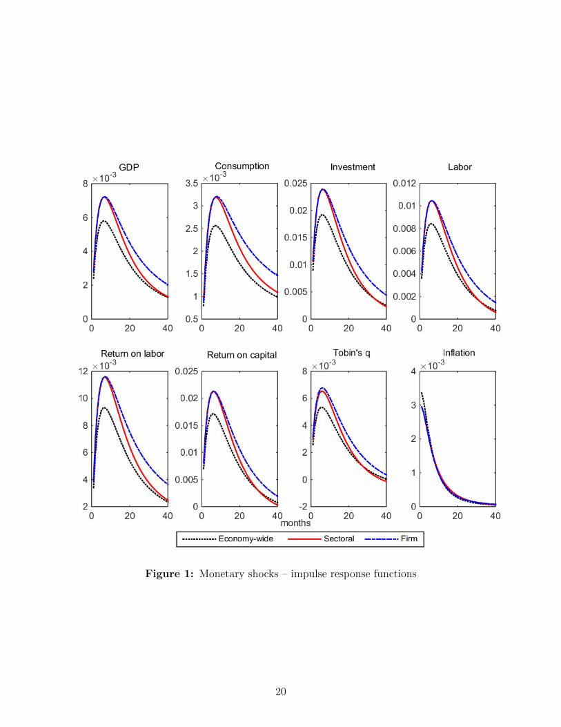
Figure 1: Monetary shocks – impulse response functions

20

Figure 2: Monetary shocks under a Taylor rule – impulse response functions

21

monetary policy with an explicit interest rate rule.30 In particular, focusing on the impulse

response functions for real GDP, the sector-specific factor model initially resembles the response

of the firm-specific factor model. Over time, its adjustment speeds up and the impulse response

function approaches that of the model with economy-wide factor markets. The real effects

of monetary shocks in the model with firm-specific factors are not only larger but also more

persistent. The same patterns hold for the remaining variables depicted in Figure 2.

Finally, in Appendix A.2 we analyze the role of the distribution of price stickiness. We

compare the dynamics of the three models under two arbitrary distributions. One represents

an economy skewed towards price flexibility and another an economy skewed towards price

rigidity. The results corroborate our discussion of Section 3 and show that, depending on the

distribution of price rigidity, the pattern of pricing interactions reflected in the NKPC under

sectoral-factor markets is rich enough to emulate the dynamics of both an economy with strong

real rigidities (such as the one with firm-specific factor markets) and an economy with strategic

substitutability in pricing decisions (such as the one with economy-wide factor markets).

5 Conclusion

Our results show that it matters a great deal whether specificity in factors of production arises

at the firm or at the sectoral level. In response to nominal shocks, our parameterized model

with sector-specific factor markets yields aggregate dynamics in the short run that resemble

those of a model with firm-specific factors. After one to two years, however, the behavior of

the model is already more similar to that of a model with economy-wide factor markets.

This result is consistent with the idea that factor price equalization might take place gradu-

ally over time, so that firm-specificity might be a reasonable short-run approximation, whereas

economy-wide markets might be a better description of how factors of production are allocated

in the longer run. Whether or not this happens in reality is, of course, an empirical question.

Existing empirical evidence that both capital (e.g., Ramey and Shapiro, 2001) and labor (e.g.,

Parent, 2000) have some degree of sector (or industry) specificity suggests that our model may

imply plausible aggregate dynamics.

Finally, one (possibly testable) implication of our parameterized model is that it behaves “as

if” its Phillips curve had a slope that is larger at higher frequencies than at lower frequencies

– when compared with the other two economies.

30Our findings about the implications of the model with sector-specific factor markets are robust to using amonetary policy rule with interest rate smoothing. The main difference relative to the results reported in Figure3 is that the overall level of persistence of real variables in response to the monetary shock is substantially lower(a result that is consistent with the findings of Carvalho and Nechio, 2015).

22

References

Altig, David, Lawrence J. Christiano, Martin Eichenbaum, and Jesper Lind. 2011.

“Firm-specific capital, nominal rigidities and the business cycle.” Review of Economic Dy-

namics, 14(2): 225 – 247.

Autor, David H., David Dorn, Gordon H. Hanson, and Jae Song. 2014. “Trade

Adjustment: Worker Level Evidence.” The Quarterly Journal of Economics, 129(4): 1799–

1860.

Ball, Laurence, and David Romer. 1990. “Real Rigidities and the Non-Neutrality of

Money.” The Review of Economic Studies, 57(2): 183–203.

Caballero, Ricardo J. 2007. “Specificity and the Macroeconomics of Restructuring.” MIT

Press.

Caballero, Ricardo J., and Mohamad L. Hammour. 1996. “On the Timing and Efficiency

of Creative Destruction.” The Quarterly Journal of Economics, 111(3): 805–852.

Caballero, Ricardo J., and Mohamad L. Hammour. 1998. “The Macroeconomics of

Specificity.” Journal of Political Economy, 106(4): 724–767.

Caballero, Ricardo J., and Mohamad L. Hammour. 2000. “Institutions, Restructuring,

and Macroeconomic Performance.” Invited Lecture at the XII World Congress of the Inter-

national Economic Association. Downloaded from http://economics.mit.edu/files/139.

Calvo, Guillermo. 1983. “Staggered Prices in a Utility Maximizing Framework.” Journal of

Monetary Economics, 12: 383–398.

Carvalho, Carlos. 2006. “Heterogeneity in Price Stickiness and the Real Effects of Monetary

Shocks.” Frontiers of Macroeconomics, 2(1): 1–58.

Carvalho, Carlos, and Fernanda Nechio. 2015. “Monetary Policy and Real Exchange Rate

Dynamics in Sticky-Price Models.” Federal Reserve Bank of San Francisco Working Paper

Series 2014-17.

Carvalho, Carlos, and Jae Won Lee. 2011. “Sectoral price facts in a sticky-price model.”

Federal Reserve Bank of New York Staff Reports 495.

Chari, V. V., Patrick J. Kehoe, and Ellen R. Mcgrattan. 2000. “Sticky Price Models

of the Business Cycle: Can the Contract Multiplier Solve the Persistence Problem?” Econo-

metrica, 68(5): 1151–1179.

23

Davis, Steven J., and John Haltiwanger. 1992. “Gross Job Creation, Gross Job Destruc-

tion, and Employment Reallocation.” The Quarterly Journal of Economics, 107(3): 819–863.

Dix-Carneiro, Rafael. 2014. “Trade Liberalization and Labor Market Dynamics.” Economet-

rica, 82(3): 825–885.

Hobijn, Bart. 2012. “The industry-occupation mix of U.S. job openings and hires.” Federal

Reserve Bank of San Francisco Working Paper Series 2012-09.

Hobijn, Bart, and Fernanda Nechio. 2015. “Sticker shocks: using VAT changes to estimate

upper-level elasticities of substitution.” Federal Reserve Bank of San Francisco Working Paper

Series 2015-17.

Justiniano, Alejandro, Giorgio E. Primiceri, and Andrea Tambalotti. 2010. “Invest-

ment shocks and business cycles.” Journal of Monetary Economics, 57(2): 132–145.

Kimball, Miles S. 1995. “The Quantitative Analytics of the Basic Neomonetarist Model.”

Journal of Money, Credit and Banking, 27(4): 1241–77.

Klenow, Peter J., and Benjamin A. Malin. 2011. “Microeconomic Evidence on Price-

Setting.” In Handbook of Monetary Economics. Vol. 3 of Handbook of Monetary Economics,

, ed. Benjamin M. Friedman and Michael Woodford, Chapter 6, 231–284. Elsevier.

Leahy, John. 2011. “A Survey of New Keynesian Theories of Aggregate Supply and Their

Relation to Industrial Organization.” Journal of Money, Credit and Banking, 43: 87–110.

Mankiw, N. Gregory, and Ricardo Reis. 2002. “Sticky Information versus Sticky Prices:

A Proposal to Replace the New Keynesian Phillips Curve.” The Quarterly Journal of Eco-

nomics, 117(4): 1295–1328.

Nakamura, Emi, and Jon Steinsson. 2008. “Five Facts about Prices: A Reevaluation of

Menu Cost Models.” The Quarterly Journal of Economics, 123(4): 1415–1464.

Parent, Daniel. 2000. “IndustrySpecific Capital and the Wage Profile: Evidence from the

National Longitudinal Survey of Youth and the Panel Study of Income Dynamics.” Journal

of Labor Economics, 18(2): 306–323.

Ramey, Valerie A., and Matthew D. Shapiro. 1998. “Capital Churning.” Manuscript.

Downloaded from http://econweb.ucsd.edu/~vramey/research/capchrn2.pdf.

24

Ramey, Valerie A., and Matthew D. Shapiro. 2001. “Displaced Capital: A Study of

Aerospace Plant Closings.” Journal of Political Economy, 109(5): 958–992.

Reiter, Michael, Tommy Sveen, and Lutz Weinke. 2013. “Lumpy investment and the

monetary transmission mechanism.” Journal of Monetary Economics, 60(7): 821 – 834.

Sheedy, Kevin D. 2007. “Inflation Persistence When Price Stickiness Differs Between Indus-

tries.” Centre for Economic Performance, LSE CEP Discussion Papers 0838.

Sveen, Tommy, and Lutz Weinke. 2005. “New perspectives on capital, sticky prices, and

the Taylor principle.” Journal of Economic Theory, 123(1): 21 – 39.

Sveen, Tommy, and Lutz Weinke. 2007a. “Firm-specific capital, nominal rigidities, and

the Taylor principle.” Journal of Economic Theory, 136(1): 729 – 737.

Sveen, Tommy, and Lutz Weinke. 2007b. “Lumpy investment, sticky prices, and the mon-

etary transmission mechanism.” Journal of Monetary Economics, 54(Supplement): 23 – 36.

Woodford, Michael. 2003. Interest and Prices: Foundations of a Theory of Monetary Policy.

Princeton University Press.

Woodford, Michael. 2005. “Firm-Specific Capital and the New Keynesian Phillips Curve.”

International Journal of Central Banking, 1(2).

25

A Appendix

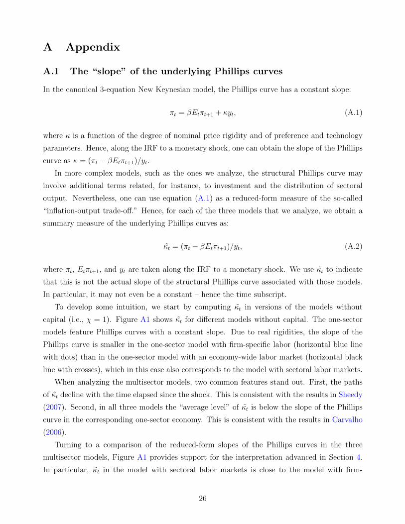
A.1 The “slope” of the underlying Phillips curves

In the canonical 3-equation New Keynesian model, the Phillips curve has a constant slope:

πt = βEtπt+1 + κyt, (A.1)

where κ is a function of the degree of nominal price rigidity and of preference and technology

parameters. Hence, along the IRF to a monetary shock, one can obtain the slope of the Phillips

curve as κ = (πt − βEtπt+1)/yt.

In more complex models, such as the ones we analyze, the structural Phillips curve may

involve additional terms related, for instance, to investment and the distribution of sectoral

output. Nevertheless, one can use equation (A.1) as a reduced-form measure of the so-called

“inflation-output trade-off.” Hence, for each of the three models that we analyze, we obtain a

summary measure of the underlying Phillips curves as:

κt = (πt − βEtπt+1)/yt, (A.2)

where πt, Etπt+1, and yt are taken along the IRF to a monetary shock. We use κt to indicate

that this is not the actual slope of the structural Phillips curve associated with those models.

In particular, it may not even be a constant – hence the time subscript.

To develop some intuition, we start by computing κt in versions of the models without

capital (i.e., χ = 1). Figure A1 shows κt for different models without capital. The one-sector

models feature Phillips curves with a constant slope. Due to real rigidities, the slope of the

Phillips curve is smaller in the one-sector model with firm-specific labor (horizontal blue line

with dots) than in the one-sector model with an economy-wide labor market (horizontal black

line with crosses), which in this case also corresponds to the model with sectoral labor markets.

When analyzing the multisector models, two common features stand out. First, the paths

of κt decline with the time elapsed since the shock. This is consistent with the results in Sheedy

(2007). Second, in all three models the “average level” of κt is below the slope of the Phillips

curve in the corresponding one-sector economy. This is consistent with the results in Carvalho

(2006).

Turning to a comparison of the reduced-form slopes of the Phillips curves in the three

multisector models, Figure A1 provides support for the interpretation advanced in Section 4.

In particular, κt in the model with sectoral labor markets is close to the model with firm-

26

Figure A1: Reduced-form slopes of Phillips curves – models without capital

Figure A2: Reduced-form slopes of Phillips curves – models with capital

27

specific labor in the short run. Later on, it approaches the value of κt in the model with an

economy-wide labor market.

While the pattern described in the previous paragraph emerges in models without capital,

Figure A2 shows that the same interpretation applies to versions of the three models of factor

specificity with both capital and labor.

A.2 Arbitrary distributions of price rigidity

Here we investigate whether the model with sectoral factor markets is indeed flexible enough

to generate either more or less monetary non-neutrality than the models with firm-specific or

economy-wide factor markets. To that end, we experiment with different arbitrary distributions

of price stickiness in economies with 3 sectors.

We entertain two alternative distributions of price rigidity. In both cases the frequencies of

price changes (αs) in sectors 1-3 are, respectively, 1, 1/12, and 1/30 – corresponding to price

changes of, on average, once a month, once a year, and once every 30 months. We differentiate

the two distributions by changing the sectoral weights.

Figure A3: IRFs of GDP to monetary shocks – arbitrary distributions of price rigidity

In the first distribution, which we term “flexible distribution,” the weights of sectors 1-3

28

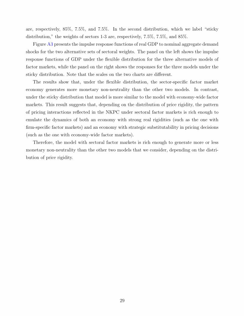
are, respectively, 85%, 7.5%, and 7.5%. In the second distribution, which we label “sticky

distribution,” the weights of sectors 1-3 are, respectively, 7.5%, 7.5%, and 85%.

Figure A3 presents the impulse response functions of real GDP to nominal aggregate demand

shocks for the two alternative sets of sectoral weights. The panel on the left shows the impulse

response functions of GDP under the flexible distribution for the three alternative models of

factor markets, while the panel on the right shows the responses for the three models under the

sticky distribution. Note that the scales on the two charts are different.

The results show that, under the flexible distribution, the sector-specific factor market

economy generates more monetary non-neutrality than the other two models. In contrast,

under the sticky distribution that model is more similar to the model with economy-wide factor

markets. This result suggests that, depending on the distribution of price rigidity, the pattern

of pricing interactions reflected in the NKPC under sectoral factor markets is rich enough to

emulate the dynamics of both an economy with strong real rigidities (such as the one with

firm-specific factor markets) and an economy with strategic substitutability in pricing decisions

(such as the one with economy-wide factor markets).

Therefore, the model with sectoral factor markets is rich enough to generate more or less

monetary non-neutrality than the other two models that we consider, depending on the distri-

bution of price rigidity.

29