factor and component analysis esp. principal component analysis (pca)

Factor and Component Analysis

esp. Principal Component Analysis (PCA)

• We study phenomena that can not be directly observed – ego, personality, intelligence in psychology– Underlying factors that govern the observed data

• We want to identify and operate with underlying latent factors rather than the observed data – E.g. topics in news articles – Transcription factors in genomics

• We want to discover and exploit hidden relationships– “beautiful car” and “gorgeous automobile” are closely related– So are “driver” and “automobile”– But does your search engine know this?– Reduces noise and error in results

Why Factor or Component Analysis?

• We have too many observations and dimensions– To reason about or obtain insights from– To visualize– Too much noise in the data– Need to “reduce” them to a smaller set of factors– Better representation of data without losing much information– Can build more effective data analyses on the reduced-

dimensional space: classification, clustering, pattern recognition

• Combinations of observed variables may be more effective bases for insights, even if physical meaning is obscure

Why Factor or Component Analysis?

• Discover a new set of factors/dimensions/axes against which to represent, describe or evaluate the data– For more effective reasoning, insights, or better visualization– Reduce noise in the data– Typically a smaller set of factors: dimension reduction – Better representation of data without losing much information– Can build more effective data analyses on the reduced-dimensional

space: classification, clustering, pattern recognition

• Factors are combinations of observed variables – May be more effective bases for insights, even if physical meaning is

obscure– Observed data are described in terms of these factors rather than in

terms of original variables/dimensions

Factor or Component Analysis

Basic Concept

• Areas of variance in data are where items can be best discriminated and key underlying phenomena observed– Areas of greatest “signal” in the data

• If two items or dimensions are highly correlated or dependent– They are likely to represent highly related phenomena– If they tell us about the same underlying variance in the data, combining them

to form a single measure is reasonable• Parsimony• Reduction in Error

• So we want to combine related variables, and focus on uncorrelated or independent ones, especially those along which the observations have high variance

• We want a smaller set of variables that explain most of the variance in the original data, in more compact and insightful form

Basic Concept• What if the dependences and correlations are not so strong or

direct?

• And suppose you have 3 variables, or 4, or 5, or 10000?

• Look for the phenomena underlying the observed covariance/co-dependence in a set of variables– Once again, phenomena that are uncorrelated or independent, and

especially those along which the data show high variance

• These phenomena are called “factors” or “principal components” or “independent components,” depending on the methods used– Factor analysis: based on variance/covariance/correlation– Independent Component Analysis: based on independence

Principal Component Analysis

• Most common form of factor analysis

• The new variables/dimensions– Are linear combinations of the original ones– Are uncorrelated with one another

• Orthogonal in original dimension space

– Capture as much of the original variance in the data as possible

– Are called Principal Components

Some Simple Demos

• http://www.cs.mcgill.ca/~sqrt/dimr/dimreduction.html

http://www.cs.mcgill.ca/~sqrt/dimr/dimreduction.html

http://www.cs.mcgill.ca/~sqrt/dimr/dimreduction.html

What are the new axes?

Original Variable A

Orig

inal

Var

iabl

e B

PC 1PC 2

• Orthogonal directions of greatest variance in data• Projections along PC1 discriminate the data most along

any one axis

Principal Components

• First principal component is the direction of greatest variability (covariance) in the data

• Second is the next orthogonal (uncorrelated) direction of greatest variability– So first remove all the variability along the first

component, and then find the next direction of greatest variability

• And so on …

Principal Components Analysis (PCA)

• Principle– Linear projection method to reduce the number of parameters – Transfer a set of correlated variables into a new set of uncorrelated

variables– Map the data into a space of lower dimensionality– Form of unsupervised learning

• Properties– It can be viewed as a rotation of the existing axes to new positions in the

space defined by original variables– New axes are orthogonal and represent the directions with maximum

variability

Computing the Components• Data points are vectors in a multidimensional space• Projection of vector x onto an axis (dimension) u is u.x• Direction of greatest variability is that in which the average

square of the projection is greatest– I.e. u such that E((u.x)2) over all x is maximized– (we subtract the mean along each dimension, and center the

original axis system at the centroid of all data points, for simplicity)– This direction of u is the direction of the first Principal Component

Computing the Components• E((u.x)2) = E ((u.x) (u.x)T) = E (u.x.x T.uT)

• The matrix C = x.xT contains the correlations (similarities) of the original axes based on how the data values project onto them

• So we are looking for w that maximizes uCuT, subject to u being unit-length

• It is maximized when w is the principal eigenvector of the matrix C, in which case– uCuT = uuT = if u is unit-length, where is the principal

eigenvalue of the correlation matrix C– The eigenvalue denotes the amount of variability captured along that

dimension

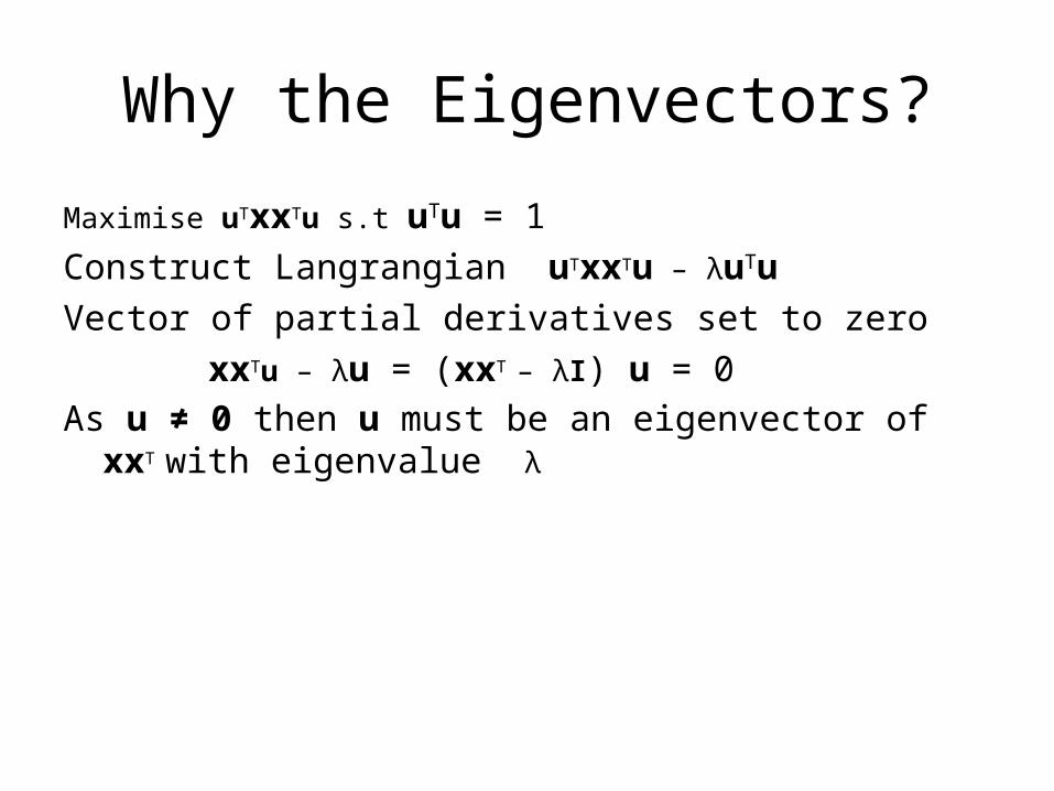
Why the Eigenvectors?

Maximise uTxxTu s.t uTu = 1

Construct Langrangian uTxxTu – λuTu

Vector of partial derivatives set to zero

xxTu – λu = (xxT – λI) u = 0

As u ≠ 0 then u must be an eigenvector of xxT with eigenvalue λ

Singular Value Decomposition

The first root is called the prinicipal eigenvalue which has an associated orthonormal (uTu = 1) eigenvector u

Subsequent roots are ordered such that λ1> λ2 >… > λM with rank(D) non-zero values.

Eigenvectors form an orthonormal basis i.e. uiTuj = δij

The eigenvalue decomposition of xxT = UΣUT

where U = [u1, u2, …, uM] and Σ = diag[λ 1, λ 2, …, λ M] Similarly the eigenvalue decomposition of xTx = VΣVT

The SVD is closely related to the above x=U Σ1/2 VT

The left eigenvectors U, right eigenvectors V, singular values = square root of eigenvalues.

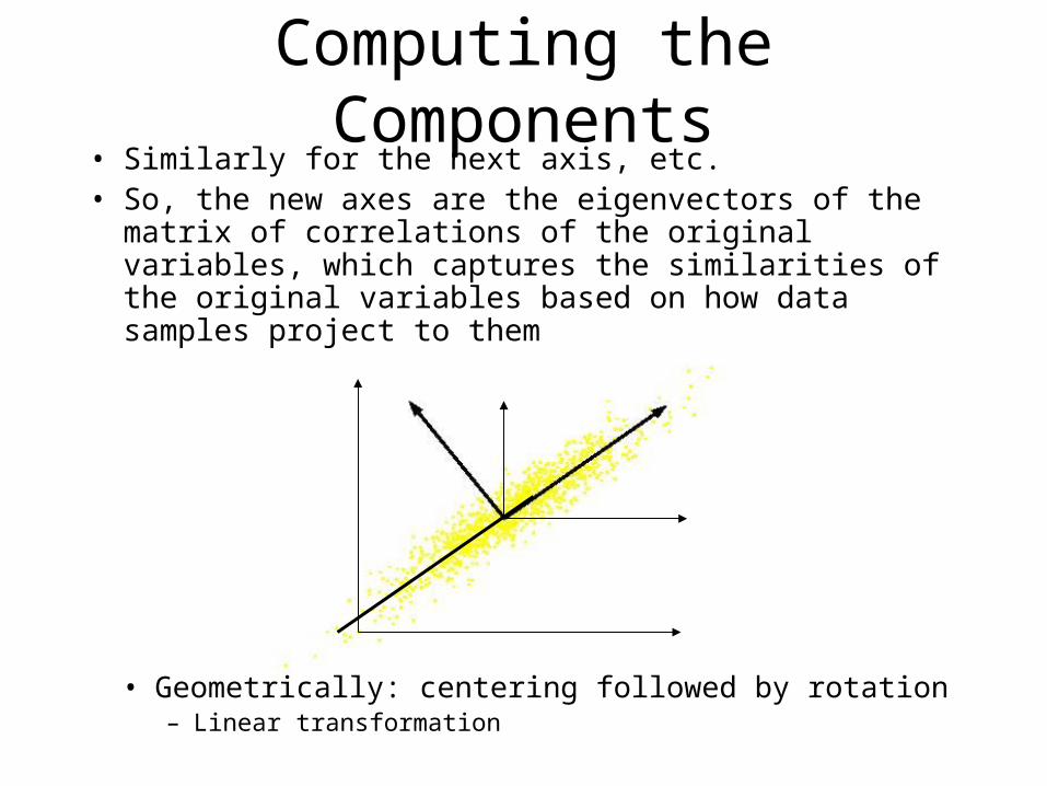
Computing the Components• Similarly for the next axis, etc. • So, the new axes are the eigenvectors of the matrix

of correlations of the original variables, which captures the similarities of the original variables based on how data samples project to them

• Geometrically: centering followed by rotation– Linear transformation

PCs, Variance and Least-Squares

• The first PC retains the greatest amount of variation in the sample

• The kth PC retains the kth greatest fraction of the variation in the sample

• The kth largest eigenvalue of the correlation matrix C is the variance in the sample along the kth PC

• The least-squares view: PCs are a series of linear least squares fits to a sample, each orthogonal to all previous ones

How Many PCs?

• For n original dimensions, correlation matrix is nxn, and has up to n eigenvectors. So n PCs.

• Where does dimensionality reduction come from?

0

5

10

15

20

25

PC1 PC2 PC3 PC4 PC5 PC6 PC7 PC8 PC9 PC10

Variance (%)

Dimensionality ReductionCan ignore the components of lesser significance.

You do lose some information, but if the eigenvalues are small, you don’t lose much– n dimensions in original data – calculate n eigenvectors and eigenvalues– choose only the first p eigenvectors, based on their eigenvalues– final data set has only p dimensions

Eigenvectors of a Correlation Matrix

Computing and Using PCA:Text Search Example

PCA/FA

• Principal Components Analysis– Extracts all the factor underlying a set of variables– The number of factors = the number of variables– Completely explains the variance in each variable

• Parsimony?!?!?!

• Factor Analysis– Also known as Principal Axis Analysis– Analyses only the shared variance

• NO ERROR!

Vector Space Model for Documents• Documents are vectors in multi-dim Euclidean space

– Each term is a dimension in the space: LOTS of them– Coordinate of doc d in dimension t is prop. to TF(d,t)

• TF(d,t) is term frequency of t in document d

• Term-document matrix, with entries being normalized TF values– t*d matrix, for t terms and d documents

• Queries are also vectors in the same space– Treated just like documents

• Rank documents based on similarity of their vectors with the query vector– Using cosine distance of vectors

Problems

• Looks for literal term matches• Terms in queries (esp short ones) don’t always capture

user’s information need well

• Problems:– Synonymy: other words with the same meaning

• Car and automobile

– Polysemy: the same word having other meanings• Apple (fruit and company)

• What if we could match against ‘concepts’, that represent related words, rather than words themselves

Example of Problems

-- Relevant docs may not have the query terms but may have many “related” terms-- Irrelevant docs may have the query terms but may not have any “related” terms

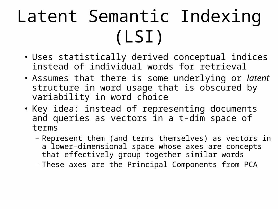
Latent Semantic Indexing (LSI)

• Uses statistically derived conceptual indices instead of individual words for retrieval

• Assumes that there is some underlying or latent structure in word usage that is obscured by variability in word choice

• Key idea: instead of representing documents and queries as vectors in a t-dim space of terms– Represent them (and terms themselves) as vectors in

a lower-dimensional space whose axes are concepts that effectively group together similar words

– These axes are the Principal Components from PCA

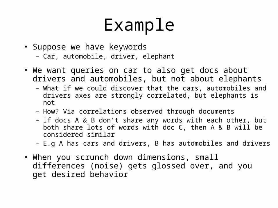
Example• Suppose we have keywords

– Car, automobile, driver, elephant

• We want queries on car to also get docs about drivers and automobiles, but not about elephants– What if we could discover that the cars, automobiles and drivers

axes are strongly correlated, but elephants is not– How? Via correlations observed through documents– If docs A & B don’t share any words with each other, but both

share lots of words with doc C, then A & B will be considered similar

– E.g A has cars and drivers, B has automobiles and drivers

• When you scrunch down dimensions, small differences (noise) gets glossed over, and you get desired behavior

LSI and Our Earlier Example

-- Relevant docs may not have the query terms but may have many “related” terms-- Irrelevant docs may have the query terms but may not have any “related” terms

LSI: Satisfying a query

• Take the vector representation of the query in the original term space and transform it to new space– Turns out dq = xq

t T -1

– places the query pseudo-doc at the centroid of its corresponding terms’ locations in the new space

• Similarity with existing docs computed by taking dot products with the rows of the matrix D2Dt

Latent Semantic Indexing

• The matrix (Mij) can be decomposed into 3 matrices (SVD) as follows: (Mij) = (U) (S) (V)t

• (U) is the matrix of eigenvectors derived from (M)(M)t

• (V)t is the matrix of eigenvectors derived from (M)t(M)• (S) is an r x r diagonal matrix of singular values

– r = min(t,N) that is, the rank of (Mij)– Singular values are the positive square roots of the eigen

values of (M)(M)t (also (M)t(M))

Example

term ch2 ch3 ch4 ch5 ch6 ch7 ch8 ch9

controllability 1 1 0 0 1 0 0 1

observability 1 0 0 0 1 1 0 1

realization 1 0 1 0 1 0 1 0

feedback 0 1 0 0 0 1 0 0

controller 0 1 0 0 1 1 0 0

observer 0 1 1 0 1 1 0 0

transfer function

0 0 0 0 1 1 0 0

polynomial 0 0 0 0 1 0 1 0

matrices 0 0 0 0 1 0 1 1

U (9x7) = 0.3996 -0.1037 0.5606 -0.3717 -0.3919 -0.3482 0.1029 0.4180 -0.0641 0.4878 0.1566 0.5771 0.1981 -0.1094 0.3464 -0.4422 -0.3997 -0.5142 0.2787 0.0102 -0.2857 0.1888 0.4615 0.0049 -0.0279 -0.2087 0.4193 -0.6629 0.3602 0.3776 -0.0914 0.1596 -0.2045 -0.3701 -0.1023 0.4075 0.3622 -0.3657 -0.2684 -0.0174 0.2711 0.5676 0.2750 0.1667 -0.1303 0.4376 0.3844 -0.3066 0.1230 0.2259 -0.3096 -0.3579 0.3127 -0.2406 -0.3122 -0.2611 0.2958 -0.4232 0.0277 0.4305 -0.3800 0.5114 0.2010

S (7x7) = 3.9901 0 0 0 0 0 0 0 2.2813 0 0 0 0 0 0 0 1.6705 0 0 0 0 0 0 0 1.3522 0 0 0 0 0 0 0 1.1818 0 0 0 0 0 0 0 0.6623 0 0 0 0 0 0 0 0.6487

V (7x8) = 0.2917 -0.2674 0.3883 -0.5393 0.3926 -0.2112 -0.4505 0.3399 0.4811 0.0649 -0.3760 -0.6959 -0.0421 -0.1462 0.1889 -0.0351 -0.4582 -0.5788 0.2211 0.4247 0.4346 -0.0000 -0.0000 -0.0000 -0.0000 0.0000 -0.0000 0.0000 0.6838 -0.1913 -0.1609 0.2535 0.0050 -0.5229 0.3636 0.4134 0.5716 -0.0566 0.3383 0.4493 0.3198 -0.2839 0.2176 -0.5151 -0.4369 0.1694 -0.2893 0.3161 -0.5330 0.2791 -0.2591 0.6442 0.1593 -0.1648 0.5455 0.2998This happens to be a rank-7 matrix

-so only 7 dimensions required

Singular values = Sqrt of Eigen values of AAT

T

Dimension Reduction in LSI

• The key idea is to map documents and queries into a lower dimensional space (i.e., composed of higher level concepts which are in fewer number than the index terms)

• Retrieval in this reduced concept space might be superior to retrieval in the space of index terms

Dimension Reduction in LSI• In matrix (S), select only k largest values• Keep corresponding columns in (U) and (V)t

• The resultant matrix (M)k is given by

– (M)k = (U)k (S)k (V)tk

– where k, k < r, is the dimensionality of the concept space

• The parameter k should be– large enough to allow fitting the characteristics of the data– small enough to filter out the non-relevant representational

detail

PCs can be viewed as Topics

In the sense of having to find quantities that are not observable directly

Similarly, transcription factors in biology, as unobservable causal bridges between experimental conditions and gene expression

Computing and Using LSI

=

=

mxnA

mxrU

rxrD

rxnVT

Terms

Documents

=

=

mxn

Âk

mxkUk

kxkDk

kxnVT

k

Terms

Documents

Singular ValueDecomposition

(SVD):Convert term-document

matrix into 3matricesU, S and V

Reduce Dimensionality:Throw out low-order

rows and columns

Recreate Matrix:Multiply to produceapproximate term-document matrix.Use new matrix to

process queriesOR, better, map query to

reduced space

M U S Vt Uk SkVk

t

Following the Example





feedback 0 1 0 0 0 1 0 0

controller 0 1 0 0 1 1 0 0

observer 0 1 1 0 1 1 0 0

transfer function

0 0 0 0 1 1 0 0

polynomial 0 0 0 0 1 0 1 0

matrices 0 0 0 0 1 0 1 1

U (9x7) = 0.3996 -0.1037 0.5606 -0.3717 -0.3919 -0.3482 0.1029 0.4180 -0.0641 0.4878 0.1566 0.5771 0.1981 -0.1094 0.3464 -0.4422 -0.3997 -0.5142 0.2787 0.0102 -0.2857 0.1888 0.4615 0.0049 -0.0279 -0.2087 0.4193 -0.6629 0.3602 0.3776 -0.0914 0.1596 -0.2045 -0.3701 -0.1023 0.4075 0.3622 -0.3657 -0.2684 -0.0174 0.2711 0.5676 0.2750 0.1667 -0.1303 0.4376 0.3844 -0.3066 0.1230 0.2259 -0.3096 -0.3579 0.3127 -0.2406 -0.3122 -0.2611 0.2958 -0.4232 0.0277 0.4305 -0.3800 0.5114 0.2010

S (7x7) = 3.9901 0 0 0 0 0 0 0 2.2813 0 0 0 0 0 0 0 1.6705 0 0 0 0 0 0 0 1.3522 0 0 0 0 0 0 0 1.1818 0 0 0 0 0 0 0 0.6623 0 0 0 0 0 0 0 0.6487

V (7x8) = 0.2917 -0.2674 0.3883 -0.5393 0.3926 -0.2112 -0.4505 0.3399 0.4811 0.0649 -0.3760 -0.6959 -0.0421 -0.1462 0.1889 -0.0351 -0.4582 -0.5788 0.2211 0.4247 0.4346 -0.0000 -0.0000 -0.0000 -0.0000 0.0000 -0.0000 0.0000 0.6838 -0.1913 -0.1609 0.2535 0.0050 -0.5229 0.3636 0.4134 0.5716 -0.0566 0.3383 0.4493 0.3198 -0.2839 0.2176 -0.5151 -0.4369 0.1694 -0.2893 0.3161 -0.5330 0.2791 -0.2591 0.6442 0.1593 -0.1648 0.5455 0.2998This happens to be a rank-7 matrix

-so only 7 dimensions required

Singular values = Sqrt of Eigen values of AAT

T

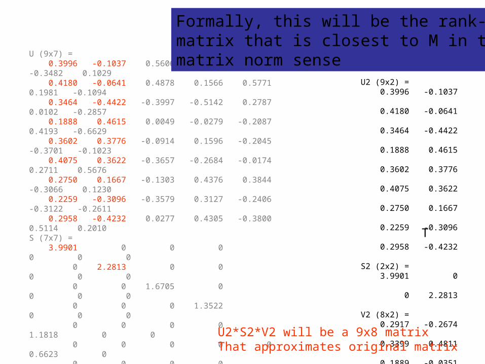
U2 (9x2) = 0.3996 -0.1037 0.4180 -0.0641 0.3464 -0.4422 0.1888 0.4615 0.3602 0.3776 0.4075 0.3622 0.2750 0.1667 0.2259 -0.3096 0.2958 -0.4232

S2 (2x2) = 3.9901 0 0 2.2813

V2 (8x2) = 0.2917 -0.2674 0.3399 0.4811 0.1889 -0.0351 -0.0000 -0.0000 0.6838 -0.1913 0.4134 0.5716 0.2176 -0.5151 0.2791 -0.2591

U (9x7) = 0.3996 -0.1037 0.5606 -0.3717 -0.3919 -0.3482 0.1029 0.4180 -0.0641 0.4878 0.1566 0.5771 0.1981 -0.1094 0.3464 -0.4422 -0.3997 -0.5142 0.2787 0.0102 -0.2857 0.1888 0.4615 0.0049 -0.0279 -0.2087 0.4193 -0.6629 0.3602 0.3776 -0.0914 0.1596 -0.2045 -0.3701 -0.1023 0.4075 0.3622 -0.3657 -0.2684 -0.0174 0.2711 0.5676 0.2750 0.1667 -0.1303 0.4376 0.3844 -0.3066 0.1230 0.2259 -0.3096 -0.3579 0.3127 -0.2406 -0.3122 -0.2611 0.2958 -0.4232 0.0277 0.4305 -0.3800 0.5114 0.2010S (7x7) = 3.9901 0 0 0 0 0 0 0 2.2813 0 0 0 0 0 0 0 1.6705 0 0 0 0 0 0 0 1.3522 0 0 0 0 0 0 0 1.1818 0 0 0 0 0 0 0 0.6623 0 0 0 0 0 0 0 0.6487V (7x8) = 0.2917 -0.2674 0.3883 -0.5393 0.3926 -0.2112 -0.4505 0.3399 0.4811 0.0649 -0.3760 -0.6959 -0.0421 -0.1462 0.1889 -0.0351 -0.4582 -0.5788 0.2211 0.4247 0.4346 -0.0000 -0.0000 -0.0000 -0.0000 0.0000 -0.0000 0.0000 0.6838 -0.1913 -0.1609 0.2535 0.0050 -0.5229 0.3636 0.4134 0.5716 -0.0566 0.3383 0.4493 0.3198 -0.2839 0.2176 -0.5151 -0.4369 0.1694 -0.2893 0.3161 -0.5330 0.2791 -0.2591 0.6442 0.1593 -0.1648 0.5455 0.2998

U2*S2*V2 will be a 9x8 matrixThat approximates original matrix

T

Formally, this will be the rank-k (2)matrix that is closest to M in the matrix norm sense





feedback 0 1 0 0 0 1 0 0

controller 0 1 0 0 1 1 0 0

observer 0 1 1 0 1 1 0 0

transfer function

0 0 0 0 1 1 0 0

polynomial 0 0 0 0 1 0 1 0

matrices 0 0 0 0 1 0 1 1





feedback 0 1 0 0 0 1 0 0

controller 0 1 0 0 1 1 0 0

observer 0 1 1 0 1 1 0 0

transfer function

0 0 0 0 1 1 0 0

polynomial 0 0 0 0 1 0 1 0

matrices 0 0 0 0 1 0 1 1

termterm ch2ch2 ch3ch3 ch4ch4 ch5ch5 ch6ch6 ch7ch7 ch8ch8 ch9ch9

controllabilitycontrollability 11 11 00 00 11 00 00 11

observabilityobservability 11 00 00 00 11 11 00 11

realizationrealization 11 00 11 00 11 00 11 00

feedbackfeedback 00 11 00 00 00 11 00 00

controllercontroller 00 11 00 00 11 11 00 00

observerobserver 00 11 11 00 11 11 00 00

transfer functiontransfer function

00 00 00 00 11 11 00 00

polynomialpolynomial 00 00 00 00 11 00 11 00

matricesmatrices 00 00 00 00 11 00 11 11

K=2

K=6

One component ignored

5 components ignored

U6S6V6T

U2S2V2T

USVT

0.52835834 0.42813724 0.30949408 0.0 1.1355368 0.5239192 0.46880865 0.5063048

0.5256176 0.49655432 0.3201918 0.0 1.1684579 0.6059082 0.4382505 0.50338876

0.6729299 -0.015529543 0.29650056 0.0 1.1381099 -0.0052356124 0.82038856 0.6471

-0.0617774 0.76256883 0.10535021 0.0 0.3137232 0.9132189 -0.37838274 -0.06253

0.18889774 0.90294445 0.24125765 0.0 0.81799114 1.0865396 -0.1309748 0.17793834

0.25334513 0.95019233 0.27814224 0.0 0.9537667 1.1444798 -0.071810216 0.2397161

0.21838559 0.55592346 0.19392742 0.0 0.6775683 0.6709899 0.042878807 0.2077163

0.4517898 -0.033422917 0.19505836 0.0 0.75146574 -0.031091988 0.55994695 0.4345

0.60244554 -0.06330189 0.25684044 0.0 0.99175954 -0.06392482 0.75412846 0.5795

1.0299273 1.0099105 -0.029033005 0.0 0.9757162 0.019038305 0.035608776 0.98004794

0.96788234 -0.010319378 0.030770123 0.0 1.0258299 0.9798115 -0.03772955 1.0212346

0.9165214 -0.026921304 1.0805727 0.0 1.0673982 -0.052518982 0.9011715 0.055653755

-0.19373542 0.9372319 0.1868434 0.0 0.15639876 0.87798584 -0.22921464 0.12886547

-0.029890355 0.9903935 0.028769515 0.0 1.0242295 0.98121595 -0.03527296 0.020075336

0.16586632 1.0537577 0.8398298 0.0 0.8660687 1.1044582 0.19631699 -0.11030859

0.035988174 0.01172187 -0.03462495 0.0 0.9710446 1.0226605 0.04260301 -0.023878671

-0.07636017 -0.024632007 0.07358454 0.0 1.0615499 -0.048087567 0.909685 0.050844945

0.05863098 0.019081593 -0.056740552 0.0 0.95253044 0.03693092 1.0695065 0.96087193

1.1630535 0.67789733 0.17131016 0.0 0.85744447 0.30088043 -0.025483057 1.0295205

0.7278324 0.46981966 -0.1757451 0.0 1.0910251 0.6314231 0.11810507 1.0620605

0.78863835 0.20257005 1.0048805 0.0 1.0692837 -0.20266426 0.9943222 0.106248446

-0.03825318 0.7772852 0.12343567 0.0 0.30284256 0.89999276 -0.3883498 -0.06326774

0.013223715 0.8118903 0.18630582 0.0 0.8972661 1.1681904 -0.027708884 0.11395822

0.21186034 1.0470067 0.76812166 0.0 0.960058 1.0562774 0.1336124 -0.2116417

-0.18525022 0.31930918 -0.048827052 0.0 0.8625925 0.8834896 0.23821498 0.1617572

-0.008397698 -0.23121 0.2242676 0.0 0.9548515 0.14579195 0.89278513 0.1167786

0.30647483 -0.27917668 -0.101294056 0.0 1.1318822 0.13038804 0.83252335 0.70210195

U4S4V4T

K=4

=U7S7V7T

3 components ignored

What should be the value of k?

Querying To query for feedback controller, the query vector would be q = [0 0 0 1 1 0 0 0 0]' (' indicates transpose),

Let q be the query vector. Then the document-space vector corresponding to q is given by: q'*U2*inv(S2) = DqPoint at the centroid of the query terms’ poisitions in the new space.For the feedback controller query vector, the result is: Dq = 0.1376 0.3678

To find the best document match, we compare the Dq vector against all the document vectors in the 2-dimensional V2 space. The document vector that is nearest in direction to Dq is the best match. The cosine values for the eight document vectors and the query vector are: -0.3747 0.9671 0.1735 -0.9413 0.0851 0.9642 -0.7265 -0.3805





feedback 0 1 0 0 0 1 0 0

controller 0 1 0 0 1 1 0 0

observer 0 1 1 0 1 1 0 0

transfer function

0 0 0 0 1 1 0 0

polynomial 0 0 0 0 1 0 1 0

matrices 0 0 0 0 1 0 1 1





feedback 0 1 0 0 0 1 0 0

controller 0 1 0 0 1 1 0 0

observer 0 1 1 0 1 1 0 0

transfer function

0 0 0 0 1 1 0 0

polynomial 0 0 0 0 1 0 1 0

matrices 0 0 0 0 1 0 1 1

termterm ch2ch2 ch3ch3 ch4ch4 ch5ch5 ch6ch6 ch7ch7 ch8ch8 ch9ch9

controllabilitycontrollability 11 11 00 00 11 00 00 11

observabilityobservability 11 00 00 00 11 11 00 11

realizationrealization 11 00 11 00 11 00 11 00

feedbackfeedback 00 11 00 00 00 11 00 00

controllercontroller 00 11 00 00 11 11 00 00

observerobserver 00 11 11 00 11 11 00 00

transfer functiontransfer function

00 00 00 00 11 11 00 00

polynomialpolynomial 00 00 00 00 11 00 11 00

matricesmatrices 00 00 00 00 11 00 11 11

-0.37 0.967 0.173 -0.94 0.08 0.96 -0.72 -0.38

U2 (9x2) = 0.3996 -0.1037 0.4180 -0.0641 0.3464 -0.4422 0.1888 0.4615 0.3602 0.3776 0.4075 0.3622 0.2750 0.1667 0.2259 -0.3096 0.2958 -0.4232

S2 (2x2) = 3.9901 0

0 2.2813

V2 (8x2) = 0.2917 -0.2674 0.3399 0.4811 0.1889 -0.0351

-0.0000 -0.0000 0.6838 -0.1913 0.4134 0.5716 0.2176 -0.5151 0.2791 -0.2591

Medline data

Within .40threshold

K is the number of singular values used

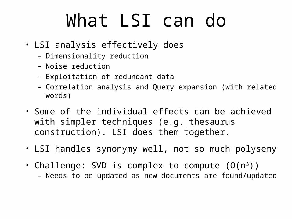
What LSI can do• LSI analysis effectively does

– Dimensionality reduction– Noise reduction– Exploitation of redundant data– Correlation analysis and Query expansion (with related words)

• Some of the individual effects can be achieved with simpler techniques (e.g. thesaurus construction). LSI does them together.

• LSI handles synonymy well, not so much polysemy

• Challenge: SVD is complex to compute (O(n3))– Needs to be updated as new documents are found/updated

SVD Properties• There is an implicit assumption that the observed data

distribution is multivariate Gaussian• Can consider as a probabilistic generative model – latent

variables are Gaussian – sub-optimal in likelihood terms for non-Gaussian distribution

• Employed in signal processing for noise filtering – dominant subspace contains majority of information bearing part of signal

• Similar rationale when applying SVD to LSI

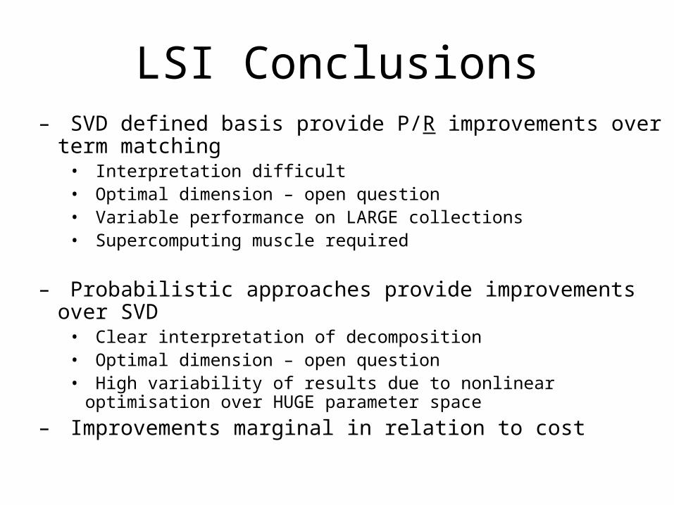
LSI Conclusions– SVD defined basis provide P/R improvements over term

matching• Interpretation difficult• Optimal dimension – open question• Variable performance on LARGE collections• Supercomputing muscle required

– Probabilistic approaches provide improvements over SVD• Clear interpretation of decomposition• Optimal dimension – open question• High variability of results due to nonlinear optimisation over HUGE

parameter space

– Improvements marginal in relation to cost

Factor Analysis (e.g. PCA) is not the most sophisticated

dimensionality reduction technique• Dimensionality reduction is a useful technique for any

classification/regression problem – Text retrieval can be seen as a classification problem

• There are many other dimensionality reduction techniques– Neural nets, support vector machines etc.

• Compared to them, LSI is limited in the sense that it is a “linear” technique– It cannot capture non-linear dependencies between original

dimensions (e.g. data that are circularly distributed).

Limitations of PCA

•Relevant Component Analysis (RCA)

•Fisher Discriminant analysis (FDA)

Are the maximal variance dimensions the relevant dimensions for preservation?

Limitations of PCA

Should the goal be finding independent rather than pair-wise uncorrelated dimensions

•Independent Component Analysis (ICA)

ICA PCA

PCA vs ICA

PCA(orthogonal coordinate)

ICA(non-orthogonal coordinate)

Limitations of PCA

• The reduction of dimensions for complex distributions may need non linear processing

• Curvilenear Component Analysis (CCA)– Non linear extension of PCA – Preserves the proximity between the points in the input

space i.e. local topology of the distribution– Enables to unfold some varieties in the input data – Keep the local topology

Example of data representation using CCA

Non linear projection of a horseshoe

Non linear projection of a spiral

PCA applications -Eigenfaces• Eigenfaces are

the eigenvectors of the covariance matrix of the probability distribution of the vector space of human faces

• Eigenfaces are the ‘standardized face ingredients’ derived from the statistical analysis of many pictures of human faces

• A human face may be considered to be a combination of these standard faces

PCA applications -Eigenfaces

To generate a set of eigenfaces:

1. Large set of digitized images of human faces is taken under the same lighting conditions.

2. The images are normalized to line up the eyes and mouths.

3. The eigenvectors of the covariance matrix of the statistical distribution of face image vectors are then extracted.

4. These eigenvectors are called eigenfaces.

PCA applications -Eigenfaces

• the principal eigenface looks like a bland androgynous average human face

http://en.wikipedia.org/wiki/Image:Eigenfaces.png

Eigenfaces – Face Recognition

• When properly weighted, eigenfaces can be summed together to create an approximate gray-scale rendering of a human face.

• Remarkably few eigenvector terms are needed to give a fair likeness of most people's faces

• Hence eigenfaces provide a means of applying data compression to faces for identification purposes.

• Similarly, Expert Object Recognition in Video

Eigenfaces

• Experiment and Results

Data used here are from the ORL database of faces. Facial images of 16 persons each with 10 views are used. - Training set contains 16×7 images.

- Test set contains 16×3 images.

First three eigenfaces :

Classification Using Nearest Neighbor• Save average coefficients for each person. Classify new face as

the person with the closest average.• Recognition accuracy increases with number of eigenfaces till 15.

　 Later eigenfaces do not help much with recognition.

Best recognition rates

Training set 99%

Test set 89%

0.4

0.6

0.8

1

0 50 100 150

number of eigenfaces

accuracy

validation set training set

PCA of Genes (Leukemia data, precursor B and T cells)

• 34 patients, dimension of 8973 genes reduced to 2

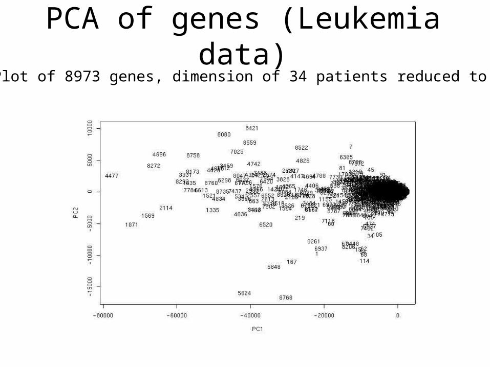
PCA of genes (Leukemia data)Plot of 8973 genes, dimension of 34 patients reduced to 2

Leukemia data - clustering of patients on original gene dimensions

Leukemia data - clustering of patients on top 100 eigen-genes

Leukemia data - clustering of genes

Sporulation Data Example

• Data: A subset of sporulation data (477 genes) were classified into seven temporal patterns (Chu et al., 1998)

• The first 2 PCs contains 85.9% of the variation in the data. (Figure 1a)

• The first 3 PCs contains 93.2% of the variation in the data. (Figure 1b)

Sporulation Data

• The patterns overlap around the origin in (1a).• The patterns are much more separated in (1b).

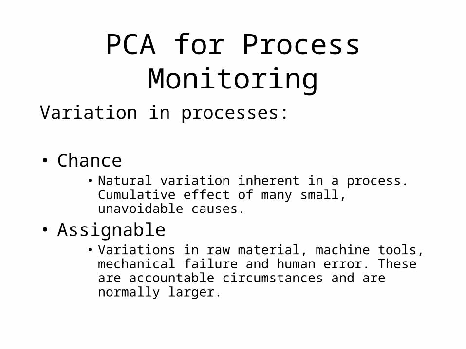
PCA for Process Monitoring

Variation in processes:

• Chance• Natural variation inherent in a process. Cumulative effect

of many small, unavoidable causes.

• Assignable• Variations in raw material, machine tools, mechanical

failure and human error. These are accountable circumstances and are normally larger.

PCA for process monitoring• Latent variables can sometimes be interpreted as

measures of physical characteristics of a process i.e., temp, pressure.

• Variable reduction can increase the sensitivity of a control scheme to assignable causes

• Application of PCA to monitoring is increasing– Start with a reference set defining normal operation

conditions, look for assignable causes– Generate a set of indicator variables that best describe the

dynamics of the process– PCA is sensitive to data types

Independent Component Analysis (ICA)

PCA(orthogonal coordinate)

ICA(non-orthogonal coordinate)

Cocktail-party Problem

• Multiple sound sources in room (independent)• Multiple sensors receiving signals which are

mixture of original signals• Estimate original source signals from mixture

of received signals• Can be viewed as Blind-Source Separation

as mixing parameters are not known

DEMO: BLIND SOURCE SEPARATION

http://www.cis.hut.fi/projects/ica/cocktail/cocktail_en.cgi

http://www.cis.hut.fi/projects/ica/cocktail/cocktail_en.cgi

• Cocktail party or Blind Source Separation (BSS) problem– Ill posed problem, unless assumptions are made!

• Most common assumption is that source signals are statistically independent. This means knowing value of one of them gives no information about the other.

• Methods based on this assumption are called Independent Component Analysis methods– statistical techniques for decomposing a complex data set into

independent parts.

• It can be shown that under some reasonable conditions, if the ICA assumption holds, then the source signals can be recovered up to permutation and scaling.

BSS and ICA

Source Separation Using ICA

W11

W21

W12

W22

+

+

Microphone 1

Microphone 2

Separation 1

Separation 2

Original　signals　(hidden　sources)　s1(t),　s2(t),　s3(t),　s4(t),　t=1:T

The ICA model

s1 s2s3 s4

x1 x2 x3 x4

a11

a12a13

a14

xi(t) = ai1*s1(t) + ai2*s2(t) + ai3*s3(t) + ai4*s4(t)

Here, i=1:4.

In vector-matrix notation, and dropping index t, this is x = A * s

This　is　recorded　by　the　microphones:　a　linear　mixture　of　

the　sources

xi(t)　=　ai1*s1(t)　+　ai2*s2(t)　+　ai3*s3(t)　+　ai4*s4(t)

Recovered　signals

BSS

• If we knew the mixing parameters aij then we would just need to solve a linear system of equations.

• We know neither aij nor si.

• ICA was initially developed to deal with problems closely related to the cocktail party problem

• Later it became evident that ICA has many other applications – e.g. from electrical recordings of brain activity from different

locations of the scalp (EEG signals) recover underlying components of brain activity

Problem:　Determine　the　source　signals　s,　given　only　the　

mixtures　x.

ICA Solution and Applicability

• ICA is a statistical method, the goal of which is to decompose given multivariate data into a linear sum of statistically independent components.

• For example, given two-dimensional vector , x = [ x1 x2 ] T , ICA

aims at finding the following decomposition

where a1, a2 are basis vectors and s1, s2 are basis coefficients.

Constraint: Basis coefficients s1 and s2 are statistically independent.

saasa

axx

222

121

21

11

2

1 ⎥⎦

⎤⎢⎣

⎡+⎥

⎦

⎤⎢⎣

⎡=⎥

⎦

⎤⎢⎣

⎡

2211 ss aax +=

Application domains of ICA

• Blind source separation • Image denoising• Medical signal processing – fMRI, ECG, EEG• Modelling of the hippocampus and visual cortex • Feature extraction, face recognition• Compression, redundancy reduction• Watermarking• Clustering• Time series analysis (stock market, microarray data)• Topic extraction• Econometrics: Finding hidden factors in financial data

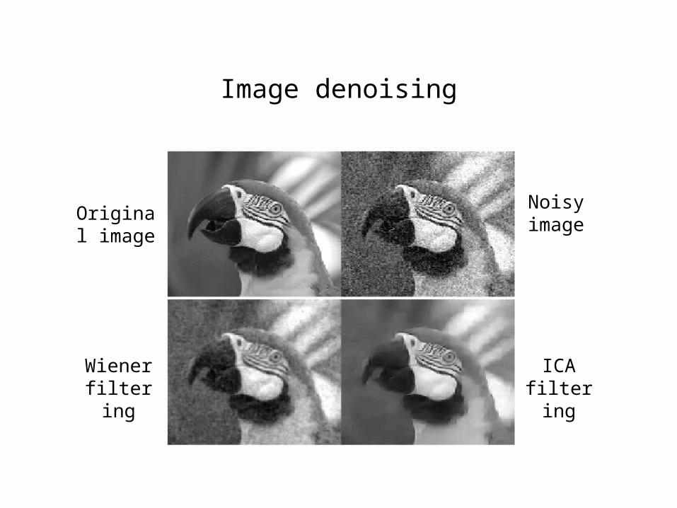
Image denoising

Wiener filtering

ICA filtering

Noisy image

Original image

Blind Separation of Information from Galaxy Spectra

0 50 100 150 200 250 300 350-0.2

0

0.2

0.4

0.6

0.8

1

1.2

1.4

Approaches to ICA

• Unsupervised Learning – Factorial coding (Minimum entropy coding, Redundancy

reduction)– Maximum likelihood learning– Nonlinear information maximization (entropy maximization)– Negentropy maximization– Bayesian learning

• Statistical Signal Processing– Higher-order moments or cumulants – Joint approximate diagonalization– Maximum likelihood estimation

Feature Extraction in ECG data (Raw Data)

Feature Extraction in ECG data (PCA)

Feature Extraction in ECG data (Extended ICA)

Feature Extraction in ECG data (flexible ICA)

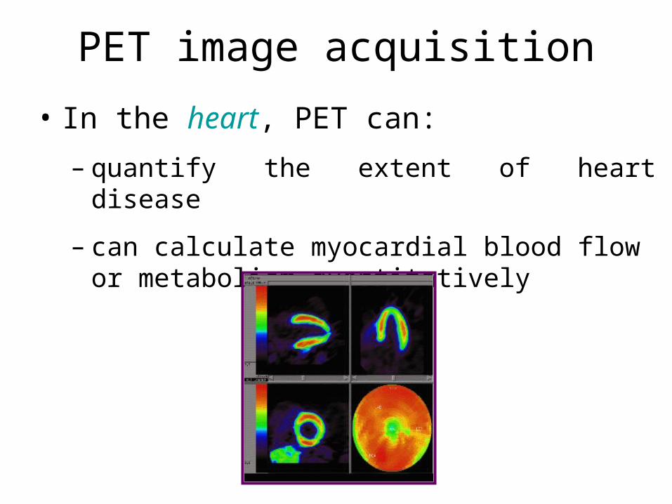
• In the heart, PET can:

– quantify the extent of heart disease

– can calculate myocardial blood flow or metabolism quantitatively

PET image acquisition

PET image acquisition

• Static image

– accumulating the data during the acquisition

• Dynamic image

– for the quantitative analysis

(ex. blood flow, metabolism)

– acquiring the data sequentially with a time interval

Dynamic Image Acquisition Using PET

tem

pora

l

spatial

frame 1

frame 2

frame 3

frame n

yN

Left Ventricle

Right Ventricle

Myocardium

Noise•　•　•

•　•　•

DynamicFrames

ElementaryActivities

IndependentComponents

•　•　•

Unmixing

•　•　•

Mixing

u1

u2

u3

uN

y1y2y3

•　•　•

g(u)

Independent Components

RightVentricle

LeftVentricle

Tissue

Other PET applications

• In cancer, PET can: • distinguish benign from malignant tumors

• stage cancer by showing metastases anywhere in body

• In the brain, PET can: • calculate cerebral blood flow or metabolism quantitatively.

• positively diagnose Alzheimer's disease for early intervention.

• locate tumors in the brain and distinguish tumor from scar tissue.

• locate the focus of seizures for some patients with epilepsy.

• find regions related with specific task like memory, behavior etc.

Factorial Faces for Recognition

Eigenfaces

Factorial　Faces

PCA/FA

Factorial　Coding/ICA

It　finds　a　linear　data　representation　thatbest　model　the　covariance　structure　of　face　image　data　(second-order　relations)

It　finds　a　linear　data　representation　thatBest　model　the　probability　distribution　of　Face　image　data　(high-order　relations)(IEEE　BMCV　2000)

Eigenfaces

PCALow　

Dimensional　Representat

ion

= a1× + a2× + a3× + a4× ++ + an×

Factorial Code Representation:Factorial Faces

Efficient Low Dimensional

Representation

PCA (Dimensionality

Reduction)

Factorial Code Representation

= b1× + b2× + b3× + b4× ++ + bn×

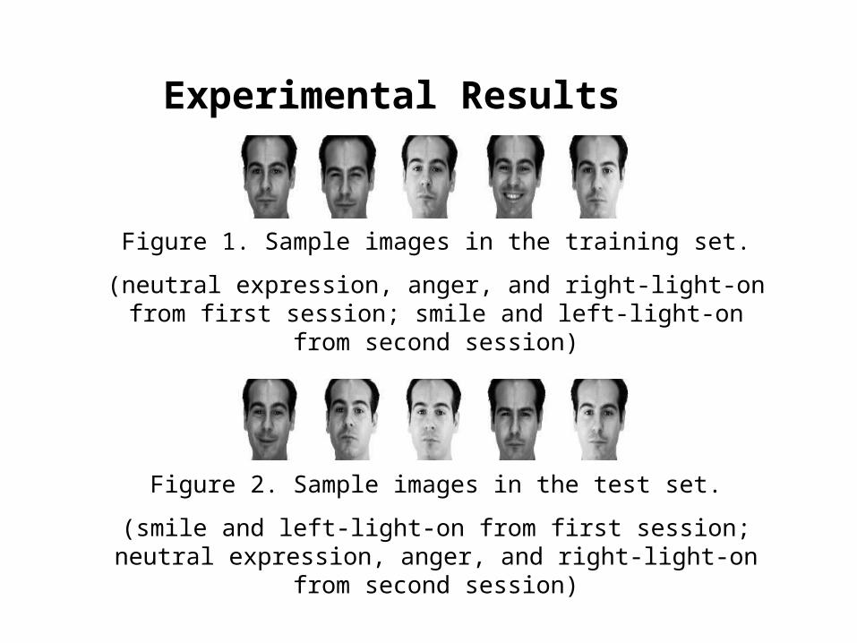
Experimental Results

Figure 1. Sample images in the training set.

(neutral expression, anger, and right-light-on from first session; smile and left-light-on from second session)

Figure 2. Sample images in the test set.

(smile and left-light-on from first session; neutral expression, anger, and right-light-on from second session)

Eigenfaces vs Factorial Faces

Figure 3. First 20 basis images: (a) in eigenface method; (b) factorial code. They are ordered by column, then, by row.

(a) (b)

Figure 1. The comparison of recognition performance using Nearest Neighbor: the eigenface method and Factorial Code Representation using 20 or 30 principal components in the snap-shot method;


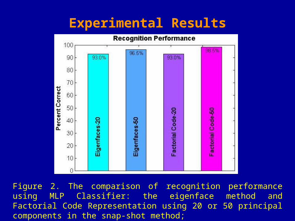
Figure 2. The comparison of recognition performance using MLP Classifier: the eigenface method and Factorial Code Representation using 20 or 50 principal components in the snap-shot method;


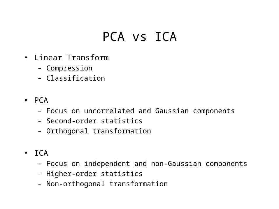
PCA vs ICA

• Linear Transform– Compression

– Classification

• PCA– Focus on uncorrelated and Gaussian components

– Second-order statistics

– Orthogonal transformation

• ICA– Focus on independent and non-Gaussian components

– Higher-order statistics

– Non-orthogonal transformation

Gaussians and ICA

• If some components are gaussian and some are non-gaussian.– Can estimate all non-gaussian components – Linear combination of gaussian components can be

estimated.– If only one gaussian component, model can be

estimated

• ICA sometimes viewed as non-Gaussian factor analysis