face recognition under angular constraint using …

FACE RECOGNITION UNDER ANGULAR CONSTRAINT USING

DISCRETE WAVELET TRANSFORM AND PRINCIPAL COMPONENT

ANALYSIS WITH SINGULAR VALUE DECOMPOSITION

BY

ENOCH SAKYI-YEBOAH

(10349736)

THIS THESIS IS SUBMITTED TO THE SCHOOL OF GRADUATE

STUDIES, UNIVERSITY OF GHANA IN PARTIAL FULFILMENT OF

THE REQUIREMENT FOR THE AWARD OF THE MASTER OF

PHILOSOPHY DEGREE IN STATISTICS

JULY 2017

University of Ghana http://ugspace.ug.edu.gh

i

DECLARATION

Candidate’s Declaration

This is to certify that, this thesis is the result of my own research work and that no part of it has

been presented for another degree in this University or somewhere else.

SIGNATURE: …………………………. DATE: ………………………..….

ENOCH SAKYI-YEBOAH

(10349736)

Supervisors’ Declaration

We hereby certify that this thesis was prepared from the candidate’s own work and supervised

in accordance with guidelines on supervision of thesis laid down by the University of Ghana.

SIGNATURE: …………………………. DATE………………………..….

DR. EZEKIEL NII NOYE NORTEY

(Principal Supervisor)

SIGNATURE: …………………………. DATE………………………..….

DR. LOUIS ASIEDU

(Co-Supervisor)


ii

ABSTRACT

The complexity of a face’s components originates from the incessant variations in the facial

component that occur with respect to time. Notwithstanding of these variations, humans recognise

a person very easily using physical characteristics such as faces, voice, gait, etc. In human

interactions, the articulation and perception of constraints; like head-poses, facial expression form

a communication channel that is additional to voice and that carries crucial information about

mental, emotional and even physical states of a conversation. Automatic face recognition deals

with extracting these essential features from an image, placing them into a suitable representation

and performing some kind of recognition on them. This study presents a statistical assessment of

the performance of modify Discrete Wavelet Transform and Principal Component Analysis with

Singular Value Decomposition (DWT-PCA/SVD) under angular constraints

(4°, 8°, 12°, 16°, 20°, 24°, 28°and 32°). 80 head-pose images from 10 individuals were captured

into the study database. The study dataset extracted from Massachusetts Institute of Technology

Database (2003-2005) were considered for recognition runs. A Friedman Sum Rank was used to

ascertain whether significant difference exist between the median recognition distances of the

varying constraints from their straight-pose ( 0°). Recognition rate and runtime was adopted as

the numerical evaluation methods to assess the performance of the study algorithm. All numerical

and statistical computations were done using Matlab. The results of the Friedman Sum Rank test

show that the higher the degrees of head-pose, the larger the recognition distances and that at 20°

and above, the recognition distances become profoundly larger compared to the 4° head-pose.

The numerical evaluations show that, DWT-PCA/SVD face recognition algorithm has an

appreciable average recognition rate (87.5%) when used to recognise face images under angular

constraints. Also the recognition rate decreases for head-poses greater than 20°. DWT is

recommended as a feasible noise removal tool that should be implemented during image pre-

processing phase.


iii

DEDICATION

This research work (thesis) is dedicated to the Almighty God, my Mother Dorcas Akosua Mansah

Adjei, my Aunt Comfort Sakyi, my Felicia Sakyi and my Dad Samuel Sakyi-Yeboah of blessed

memory.


iv

ACKNOWLEDGEMENT

My sincerest thankfulness spirits to the Almighty God for his Divine Grace, Mercy and Favour

upon my Life throughout my stay in the University of Ghana. Without Him I wouldn’t have come

this far.

I want to use this golden chance to express my considerate appreciation, sincere gratitude and

bottomless esteems to my hard working supervisors, Dr. Ezekiel Nii Noye Nortey and Dr. Louis

Asiedu for their exemplary supervision, monitoring, and continuous inspiration during the course

of this research work. From the initial stages (deciding and choosing a topic) of this research

work, to the late day of submission, I owe an immense obligation of gratitude to my distinguish

supervisors. Their sound advice, encouragement and careful guidance were invaluable.

I am indebted to Dr. Felix Okoe Mettle and Mr. Issah Seidu, for their affectionate support,

valuable information, explanation and guidance, which aided me in completing this task through

various stages of my research work.

I am very grateful to Dr. Samuel Iddi, Mrs. Charlotte Chapman Wardy, Asaa Gyebi-Adjei, Benita

Odoi, Derek K. Degbedzui, Alberta Adoma Bawuah, Jacklyn Asiedua Korankye and Abeku Atta

Asare-Kumi, for the assistances provided by them in their relevant fields. I am obliged for their

care, co-operation and support during the course of my research work.

Finally, I thank My Mother, Auntie, Sibling, Cousins, Roommates (Seth Attah Armah, Francis

Dogodzi and Kwaku Kyere Appiah) and Colleagues (Emmanuel Kojo Aidoo, Stephen Nkrumah,

Obu Amponah Amoah, Fred Fosu Agyarko, Millicent Narh) for their constant encouragement

and support, without which this research work would not have been possible.

Thank you all for this immeasurable support. May the Almighty richly bless you all in abundant.


v

TABLE OF CONTENT

Contents

DECLARATION ............................................................................................................................ i

ABSTRACT ...................................................................................................................................ii

DEDICATION ............................................................................................................................. iii

ACKNOWLEDGEMENT ............................................................................................................ iv

TABLE OF CONTENT ................................................................................................................. v

LISTS OF FIGURES ................................................................................................................. viii

LISTS OF PLATES ...................................................................................................................... ix

LISTS OF TABLES ....................................................................................................................... x

ABBREVIATION......................................................................................................................... xi

CHAPTER ONE ............................................................................................................................ 1

INTRODUCTION ......................................................................................................................... 1

1.1 Background of the Study ...................................................................................................... 1

1.2 Problem Statement ............................................................................................................... 4

1.3 Objectives ............................................................................................................................. 5

1.4 Significance of the Study ..................................................................................................... 5

1.5 Brief Methodology ............................................................................................................... 6

1.6 Scope .................................................................................................................................... 7

1.7 Limitation of the study ......................................................................................................... 7

1.8 Analytic Tools Used for the Study ....................................................................................... 7

1.9 Organization of the study ..................................................................................................... 7

CHAPTER TWO ........................................................................................................................... 9

LITERATURE REVIEW .............................................................................................................. 9

2.1 Introduction .......................................................................................................................... 9

2.2 Reviews of Face Recognition Works ................................................................................... 9

2.2.1 Face Recognition Approaches ..................................................................................... 13


vi

2.2.2 Face Recognition Techniques ...................................................................................... 14

2.3 Feature Extraction Method ................................................................................................. 15

2.4 Haar Transform .................................................................................................................. 26

2.5 Conclusion .......................................................................................................................... 30

CHAPTER THREE ..................................................................................................................... 31

METHODOLOGY ...................................................................................................................... 31

3.1 Introduction ........................................................................................................................ 31

3.1.1 Data Acquisition .......................................................................................................... 31

3.2 RECOGNITION PROCEDURE ........................................................................................ 32

3.2.1 Preprocessing Stage ..................................................................................................... 32

3.2.2 Feature Extraction Technique ...................................................................................... 42

3.2.3 Recognition Stage ........................................................................................................ 47

3.3 Statistical Testing Approach .............................................................................................. 49

3.3.1 Assessing Multivariate Normality Based on the Euclidean Distance ......................... 50

3.3.2 Repeated Measures Design .......................................................................................... 52

3.3.3 Friedman Rank Sum Test ............................................................................................ 55

CHAPTER FOUR ........................................................................................................................ 60

DATA ANALYSIS ...................................................................................................................... 60

4.1 Introduction ........................................................................................................................ 60

4.1.1 Data Description .......................................................................................................... 60

4.2 Result .................................................................................................................................. 61

4.2.1 Preprocessing Stage ..................................................................................................... 61

4.2.3 Feature Extraction Stage .............................................................................................. 63

4.2.3 Recognition Procedure Stage....................................................................................... 69

4.3 Statistical Evaluation of the Euclidean Distance................................................................ 70

4.3.1 Assessing for Normality .............................................................................................. 70

4.3.2 Test for Multivariate Normality .................................................................................. 71


vii

4.3.3 Friedman Rank Sum Test ............................................................................................ 72

4.3.4 Recognition Rate ......................................................................................................... 73

4.3.5 Recognition Curve ....................................................................................................... 74

CHAPTER FIVE ......................................................................................................................... 76

Summary, Conclusion and Recommendation .............................................................................. 76

5.1 Introduction ........................................................................................................................ 76

5.2 Summary ............................................................................................................................ 76

5.3 Conclusions and Recommendations................................................................................... 77

REFERENCE ............................................................................................................................... 78

APPENDIX I ............................................................................................................................... 85

APPENDIX II .............................................................................................................................. 87


viii

LISTS OF FIGURES

Figure 3.1: Research Design ........................................................................................................ 32

Figure 3.2: Summary of face recognition process of the study ................................................... 48

Figure 4.1: A display of covariance matrix of the train image .................................................... 64

Figure 4.2: Image unit of eigenvector U ...................................................................................... 66

Figure 4.3: Image of the diagonal matrix of the train image ....................................................... 66

Figure 4.6: Proportion of the variance explained by the principal components .......................... 67

Figure 4.4: A graph of observed data quantiles against the normal quantiles ............................. 72

Figure 4.5: Displayed the recognition curve ................................................................................ 75

This implies that adopting a DWT-PCA/SVD algorithm, the recognition rate decline for the

varying angular constraint above 20 . ......................................................................................... 75


ix

LISTS OF PLATES

Plate 3.1: Original images generated from 3D models for all ten subject ................................... 31

Source: [Weyrauch, Huang, Heisele & Blanz (2004)] ................................................................ 31

Comprehensive description of the data used has been presented in the subsequent chapter

(Chapter 4). .................................................................................................................................. 31

Plate 4.1: The display of the ten train image ............................................................................... 60


Plate 4.2: Example of the test image under the various angular pose.......................................... 61


Plate 4.3: Preprocessed image from DWT ................................................................................... 63

Plate 4.4: Image of the eigenface of the trained image ................................................................ 68

Plate 4.5: Example of correctly recognised individual across all angular poses ........................ 75



x

LISTS OF TABLES

Table 1.1: consist of some application to face recognition system................................................ 6

Table 3.1: Discrete Wavelet Transform decomposition of an image using 3-level pyramid where

1, 2, 3 represent Decomposition levels, H represent High Frequency Bands and L represent Low

Frequency Bands .......................................................................................................................... 36

Table 3.2: Data display for the Friedman Two-Way Anova by ranks ......................................... 57

Table 4.1: The euclidean distance for the ten image in the train dataset. .................................... 70

Table 4.3: Friedman Test ............................................................................................................. 72

Table 4.4: Pairwise comparisons (Post hoc of the Friedman Test).............................................. 73

Table 4.5: Recognition Rate ........................................................................................................ 74


xi

ABBREVIATION

AFR……………………………… Automatic Face Recognition

ANN……………………………… Artificial Neural Network

BFLD …………………………… Block-based Fisher’s linear discriminant

BFR……………………………… Biometric Face Recognition

CWT…………………………… Continuous Wavelet Transform

DFT…………………………… Discrete Fourier Transform

DLDA………………………... Direct Linear Discriminant Analysis

DWT. ………………………… Discrete Wavelet Transform

FFT…………………………… Fast Fourier Transform

FRVT…………………………. .Face Recognition Vendor Tests

FWT ………………………… Fast Wavelet Transform

GF…………………………… Gabor Feature

IALDA………………………… Illumination Adaptive Linear Discriminant Analysis

ICA……………………………. Independent Component Analysis

ID……………………………… Identification Number

IDWT………………………… Inverse Discrete Wavelet Transform

KLT………………………….. Karhumen-Loeve transformation

KPCA………………………… Kernel Principal Component Analysis

LDA…………………………... Linear Discriminant Analysis


xii

LFA…………………………… Local Feature Analysis

LMBP…………………………….. Levenberg-Marquardt backpropagation

MIT…………………………… Massachusetts Institute of Technology

MPCA………………………… Modified Principal Component Analysis

MRA…………………………… Multiresolution Analysis

MVN…………………………... Multivariate Normality

NDA…………………………… Non-Parametric Discriminant Analysis

PCA…………………………… Principal Component Analysis

PDF……………………………. Probability Distribution Function

PINS…………………………… Person Identification Number

SURF…………………………... Speeded Up Robust Feature

SVD……………………………. Singular Value Decomposition

SVM…………………………… Support Vector Machine

WHT…………………………. Walsh-Hadamard Transform

WMPCA……………………. Weighted Modular Principal Component Analysis


1

CHAPTER ONE

INTRODUCTION

1.1 Background of the Study

The human brain has a sensory organ (specialised nerve cells) that permit an individual’s to

recognise features such as angles, lines, edges or movement. These nerve cells operate 24 hours

after birth (Wagner, 2012). However, the complexity of a face’s components originates from the

incessant variations in the facial component that occur with respect to time. Notwithstanding of

these variations, humans recognise a person very easily using physical characteristics such as

faces, voice, gait, etc. Automatic face recognition deals with extracting these essential features

from a face image, placing them into a suitable representation and executing some kind of

recognition on them (Wagner, 2012). The knowledge of mimicking this skill characteristic in

individuals by machines can be very worthwhile, however the innovation emerging from an

intelligent and self-learning system may necessitate the provision of adequate data for the

machine to operate. A well-organised and robust face recognition technique is valuable in a

number of application areas. These include, criminal identification, access management, law

enforcement, information security and entertainment or leisure. Recently, Face recognition has

become a relevant technique that we employ in our day by day lives and this has received

blooming attention among researchers and the general public. This can be attributed to its

application in various areas such as terrorisms, robberies, thefts, assassinations, mob justice,

credit card fraud, etc., committed across the globe. Albeit, researchers argued that face

recognition is the most challenging problem associated with computer vision and posited that face

recognition applications are far from restricted to security system as perceived and portrayed by

the general public (Sahu and Tiwari, 2015).


2

The primary aim of using a face recognition framework is for both verification (of this situation,

the framework essentials affirm or dismiss the identity of the individual in the query database

“input face”) and identification (in this situation, the framework consist of unidentified face, and

this process report back to determine identity from a database of identifying faces) purposes.

For many years, people have been utilizing physical human attributes, for example, gait

(movement), facial expression, voice, height, weight, shadow and many more mechanisms to

recognise an individual. The set of facial features that relate to an individual constitutes their

respective identity. With the introduction of computers in the nineteenth century, the scientific

community was interested in using computer software applications to identify or verify an

individual’s identity. This led to face recognition studies which present an individual facial image

with targeted facial characteristics (such as the mouth, eye, ear and nose) and tends to measure a

face image at a time.

The process of using face recognition, works with individuals’ images in addition to tackling

many stimulating real-world uses such as de-duplication of identity documents (for example,

National Health Insurance Scheme , passport, voter ID, driver license, national ID and many

others), access control and video surveillance (Liao, Jain, & Li, 2013).

Chellappa, Wilson, and Sirohey (1995) and Woodward Jr, Horn, Gatune, and Thomas (2003) in

their respective research findings, concluded that face recognition is a fundamental part of

biometrics, which aids the automatic recognition of an individual utilizing recognised traits of the

same individual.

The face recognition techniques involve two ways which are based on the various criteria,

namely; an appearance-based model (could also refer as photometric-based) and feature-based

(could also be refer as geometrical-based) model. The appearance-based model utilises the entire

or specific areas of the face for recognition and verification. The application of appearance-based


3

model is achieved by extracting the facial feature from the facial image. The feature-based uses

the geometrical components of the face images which includes the position of the ear, mouth, eye

and nose. The feature-based focus on assessing the geometric distance among the position of eyes,

ratio of geometric distance among the position of the nose and eye. Thus, face recognition which

employs feature-based model of a face image is presumably the natural way to deal face

recognition.

Current researchers revealed that there are two approaches in the face recognition system: the

first approach is the face recognition framework which utilises facial characteristics such as

mouth, eye, nose, ear and chin to recognise an image; the second approach utilises the entire face

to recognise an individual image. In the first approach, Belhumeur, Jacobs, Kriegman, and Kumar

(2013) portrayed that the local method of face recognition calculates the descriptor of the facial

characteristics of the face image and assembles images into a single descriptor. Some examples

of the feature-based methods are: Local Feature Analysis (LFA), Garbor Features (GF), Elastic

Bunch Graph Matching (EBGM) and Local Binary Pattern Feature (LNPF). In the second

approach, the idea of the entire face technique is to develop a subspace using Principal

Component Analysis (PCA), Linear Discriminant Analysis (LDA), Independent Component

Analysis (ICA) and Random Projection (RP) or Non-negative Matrix Factorization (NMF) as a

feature extraction technique. These dimensionality reduction (mainly feature extraction)

techniques lessen the huge dimensional space of the face image information (matrix) to an

intrinsic low dimensional space with approximately the same face image information for

recognition purposes (Belhumeur et al., 2013).

Wagner (2012) stated that the automatic face recognition approach utilised the extracted features

of a face image. Thus putting the face images into a vital representation of the extracted facial

feature and performing the recognition. This kind of approach improves the recognition rate of

face recognition systems. Liao et al. (2013) argued that despite the fact that the automatic face


4

recognition algorithm has improved recognition rate significantly, there exist many problems

associated to the performance of a face recognition algorithm under environmental constraint

(which involves facial expression, pose variation, occlusion, ageing and extreme ambient

illumination). Also, developing an algorithm for a face recognition system is quite a challenging

task since human faces are multifaceted, multi-dimensional and react to visual stimuli (Sahu &

Tiwari, 2015) . Many researchers have designed an algorithm to tackle face recognition problems,

but there is little work on face recognition under angular constraint. Lately, angular constraints

have generated a lot discussion among the scientific community. Since the face images captured

by any digital devices are somehow tilted, many researchers have advocated for extensive

research work directed towards angular constraints. The study focused on recognizing face

images under angular constraints using DWT-PCA/SVD algorithm.

1.2 Problem Statement

The problems associated with face recognition continue to attract researchers from various

disciplines due to the numerous application of face recognition. Currently, face recognition is

categorised on model based schemes which are derived from the number of typical algorithm

presented. Weyrauch, Heisele, Huang, and Blanz (2004) posited that, variations in the frontal

view pose mainly lead to the variations in the position of the facial component which called for

the flexibility of the geometric model. Murugan, Arumugam, Rajalakshmi, and Manish (2010)

stated that after many years of invention of various software packages and exploration, face

recognition remains a challenging field of study. The authors argued that face recognition are

sensitive to variation based on an individual image pose position. Passalis, Perakis, Theoharis,

and Kakadiaris (2011) presented a three-dimension model to tackle frontal head pose of the face

recognition algorithm. Their study revealed that angular constraints pose a great challenge to face

recognition algorithm especially in real-world biometric applications. Beham and Roomi (2012)


5

suggested that there are numerous issues that requires an extensive research in the area of face

recognition algorithm. These issues also speak to the need for further improvement in facial

recognition to address challenges of angular variation.

This study will try to fill the gap by assessing the performance of a modified algorithm (DWT-

PCA/SVD) under angular constraints.

1.3 Objectives

This study measure the performance of a modified face recognition algorithm (DWT-PCA/SVD)

under angular constraints. Specifically the study seeks to;

i. Modify PCA/SVD algorithm using DWT at preprocessing phase.

ii. Assess whether a significance difference exists in the average recognition distance of the

various angular constraints.

iii. Assess the performance of the modified algorithm under angular constraints through the

computation of the recognition rate.

1.4 Significance of the Study

An efficient and resilient face recognition algorithm is significant in addressing most of the real

life problems in application areas displayed in Table (1.1).

Thus, this study serves as a catalyst to breed interest and further research into the other aspects of

biometrics in Ghana.


6

Table 1.1: consist of some application to face recognition system

1.5 Brief Methodology

The study used a secondary database which was extracted from Massachusetts Institute of

Technology (2003-2005) Database. This database consists of various angular faces of ten

individuals (both male and female) in a morphable model. The angular face image data served as

an input for the proposed model. Ten face images from 10 individuals with head pose (0°) were

captured into the training image database to be trained by the study algorithm. The test image

database consist of 80 face images from 10 individuals each of which is captured under eight

angular constraints ( 4°, 8°, 12°, 16°, 20°, 24°, 28°and 32°). The facial image of these individuals

were captured and resized to 100 × 100 pixel resolution dimension for the recognition.

Areas Application of Face Recognition

Information Security

Accessing Security, Data Privacy, User authentication, Intranet security,

Application security, File encryption, Securing trading terminal, Medical

records, Internet access, TV-Parental control, Personal device log on,

Access Management Secure Access Authentication,

Biometric

Personal Identification (National ID, Passport, Driver’s licenses,)

Welfare fraud, Entitlement programs Immigration, voter registration,

multimedia communication (synthetics face),

Law Enforcement

Advanced Video surveillance, Forensic Reconstruction of Face remains,

CCTV Control, Portal control, Post event analysis, Ship lifting, Suspect

trading and Investigation

Entertainment, Leisure

Virtual reality, Photo camera, Training program, Human-robot

interaction, Human-computer-interaction and home video games


7

Several literatures have revealed that face recognition is executed in three essential phases,

namely the pre-processing phase, extraction (dimension reduction) of facial features phase and

classification (recognition) stage. The research focused on running a template-based (DWT-

PCA/SVD) face recognition algorithms which is constructed on a face frontal database and

subsequently evaluated the performance of the study algorithm for recognition.

1.6 Scope

The study relies on recognizing the frontal face images in the adopted database under varying

head pose.

1.7 Limitation of the study

This study is limited to assessment under angular constraints.

Face images captured under any other constraints except the aforementioned were not

considered in the study.

1.8 Analytic Tools Used for the Study

The analytical tool that was used for the image training and recognition is the Matlab [version

R2015a]. The Matlab software was also used for all numerical computation.

Also, R software was used for all statistical analysis.

1.9 Organization of the study

The study of face recognition under angular constraints using DWT-PCA/SVD consist of five

chapters. The first chapter consists of an introduction of the study, which involves background of

the study, problem statement, objectives, the significance (some application of the face

recognition system), brief methodology, scope of the study, limitation, analytic software used and

chapter organization including general overview of face recognition algorithm used.

The Chapter Two covers empirical and theoretical review of articles, journals and related issues

on face recognition. This includes an automatic face recognition techniques and approaches

involving the PCA/SVD and wavelet transform.


8

Chapter Three provides concrete theories and the underlying assumption that was employed in

this study. This chapter entails the discussion of Discrete Wavelet Transform and Principal

Component Analysis with Singular Value Decomposition (DWT-PCA/SVD) in face recognition

stages. The chapter also discusses the preprocessing techniques, recognition procedure and

feature extraction methods in face recognition algorithm.

In Chapter Four, the study presents the analysis of the data results and discussion on facial

recognition system. A computational model for the frontal view of images which is based on

statistical technique is developed. The PCA/SVD was modified and evaluated under angular

constraints using MIT database. The frontal view of face recognition algorithms is extended to

angular constraint.

Chapter Five presents the findings, conclusions and recommendation of the study.


9

CHAPTER TWO

LITERATURE REVIEW

2.1 Introduction

This chapter focuses on the empirical and theoretical appraisal of articles, journals and related

issues on face recognition using Discrete Wavelet Transform and Principal Component Analysis

with Singular Value Decomposition (DWT-PCA|SVD). This includes an automatic face

recognition techniques and approaches involving the PCA|SVD, wavelet transform and other

statistical approach.

2.2 Reviews of Face Recognition Works

The earliest study of face recognition can be traced as far back as the 1870s. Darwin (1872)

initiated the earliest studies in the works on facial expression of emotions in man and animals.

Galton (1892) works on facial profile-based biometrics aimed at personal identification. The

study discovered an independent feature suitable for hereditary investigation that aided personal

identification. The study was limited to parentage and next of kingship, but failed to address the

variation in similarity image, pose, illumination, occlusion, etc. It was also around the 1950’s that

automated face recognition was developed.

Bruner and Tagiuri (1954) pioneered the first research studies into the automated face recognition

system in a psychology research. In engineering, Bledsoe (1964) adopted existing literature

methods to design and implement a semi- automated system. The short-comings were attributed

to recognition on a huge database of face images and photographs. The challenge was to select a

small set of records from the image database such that one of the image records matched the

photograph. In addition, Bledsoe’s work received a little publicity due to the fact that the work

was fully funded by an unnamed intelligence agency.

In 1970s, Kelly (1970) and Kanade (1973) presented seminars in which an semi-automated face

recognition technique were adopted to map a person’s face image onto a global template using a


10

facial template scheme. However, their method required high computational time because

locations and measurements were done manually. Literature revealed that after the studies of

Kelly (1970) and Kanade (1973), research work related to face recognition system became

dormant until the mid-1980s, when researchers concentrated on automated face recognition

techniques which employed facial component (such as the eye, nose and mouth) to recognise an

individual image. Sirovich and Kirby (1987) initiated the methods of representing a facial image

in a picture format (dimension). Their study indicates that within a specified framework, a face

represented in a picture form is unique. Further, they also stated that the characterization of a

face, within an error bound of relative low dimensional vectors, is limited when significant scale

and illumination variation are present. Kohonen (1989) used simple neural networks to perform

face recognition for aligning and normalizing face images. Their study employed computer face

descriptor to approximate the eigenvectors of the face image autocorrelation matrix. Kohonen’s

procedure seemed good because of the need for precise alignment and normalization, but his

procedure was practically unsuccessful.

Later in the 1990’s, face recognition techniques saw a perceptible upsurge in the number of

articles and journals in various research blogs. The design of different algorithms to evaluate face

recognition have emerged from various disciplines such as Engineering (Electrical & Computer),

Mathematics, Statistics, Computer Science, Psychology, etc. Among them are PCA, ICA, LDA,

Neural Network and their derivatives (Asiedu, Adebanji, Oduro, & Mettle, 2015). Kirby and

Sirovich (1990) focused on a well-defined human face and employed the Karhunen–Loeve

Transform (KLT) expansion framework. This approach was classified as unsuccessful as it

proved that fewer than 100 values were essential to precisely code suitably aligned and

normalised images. The outcome of the study projected face onto an optimal basis. The shortfall

of this study is that Eigen function of the covariance matrix was manually computed.


11

Turk and Pentland (1991) states that the application of the information theory motivated their

study to adopt an eigenface approach to provide practical solutions to face recognition problem.

The eigenface approach adopted to face recognition is relatively simple, very fast and performed

better under constrained environment. Even though the eigenface approach was restricted by

constrained environment, it still created significant framework in advancing the developments of

automatic face recognition systems.

The development stage for face recognition began a century ago, but it was made available

commercially in the 1990’s. Public attention was drawn to the trial version of face recognition

technology in January 2001 at USA Super Bowl event. During the Super Bowl event, surveillance

face images were captured and compared to digital mugshot database. Research revealed that

many people across the globe heard of the face recognition technologies after September 11 th,

2001 disaster (Vijg, 2011).

In 2006, the National Science and Technology Council (NSTC) report revealed that face

recognition technology was first introduced at the 2004 Super Bowl event. This work, involving

face recognition technologies, initiated an ultimate attention on the technology to support natural

needs while being considerate of public social and privacy concern.

Recent years have countersigned an emergent concentration of researchers in the field of face

recognition. The significant attentiveness is based on the increasing application areas of the face

recognition system. Among these application areas are the Information Security (Data privacy,

User authentication), Biometric system (National IDs, Passport checks, School ID, Staff ID, etc.),

Law enforcement agency (video surveillance, forensic reconstruction of face, criminal

investigation, etc.), and Image and Film processing. The ability of a face recognition system to

suitably recognise the face image depends on a variation of variables, including illumination,

head pose, lighting (Gross & Brajovic, 2003), expressions of the facial features (Georghiades,


12

Belhumeur, & Kriegman, 2001), quality of the image (Shan, Gong, & McOwan, 2009) and tilted

angular image.

Currently, face recognition technologies are used to combat crime such as passport fraud,

credit/debit card fraud, support law enforcement, identify missing individuals and reduce

benefit/identity fraud. It is also an undeniable fact that many researchers have addressed the

problems associated with face recognition; by proposing various types of algorithms and

techniques which are equivalent to the ability of the human brain (from different point of views).

Face recognition algorithms are classified into two categories: image template-based or geometry

feature-based. The geometric featured-based method analyses the localised facial component and

establishes a geometrical relationship. The geometrics facial features includes that eye brow,

mouth, chin, cheeks, etc. A typical example of this method is the Elastic Bunch Graph Modelling

algorithm.

Carrera and Marques (2010) stated that geometric approach employed a set of fiducial point for

face recognition. The geometric features are generated by segments, perimeters and some areas

by the fiducial points. However, this approach is less often used since there are developed

algorithm that use the whole face (template-based) approach. The Template-based methods

(Appearance-based method) utilise the facial feature of the entire face to perform face

recognition. Template-based methods calculates a measure of correlation between original faces

and a set of template models to assess the face identity (Guillamet & Vitria, 2002). Independent

Component Analysis (ICA), Linear Discriminant Analysis (LDA), Principal Component Analysis

(PCA), Singular Value Decomposition (SVD) and the Non-Negative Matrix Factorization (NMF)

are some example of template based method.

These algorithms are typically dimensional reduction (feature extraction technique) algorithms

which seek to lessen the dimensions of the face space, thereby bringing out only important points


13

on the face for recognition and identification purposes. In face recognition works, the dimension

of the face images are very huge and this requires a substantial amount of computational time

(runtime) for recognition (classification) (Thakur, Sing, Basu, Nasipuri, & Kundu, 2008).

2.2.1 Face Recognition Approaches

According to Brunelli and Poggio (1993) and N. A. Singh, Kumar, and Bala (2016) there are

three face recognition approaches namely:

Geometrical (feature) based approach

Holistic based approach

Hybrid approach

2.2.1.1 Face Recognition using Features Based Approach

The method of using geometrical features in face recognition implies that recognition of facial

components such as nose, eye and hair. These facial components are partitioned into segments

for faster and easy recognition of a face image. The process uses an input data for recognition of

face image by matching input images with available database images.

For the feature component-based methods, the fundamental principle is to recompense for pose

variations by permitting a flexible geometrical relation among the features in the recognition

phase (Reddy, Babu, & Kishore, 2011). Brunelli and Poggio (1993) performed a face recognition

task by adopting a matching template of facial features (eye, nose and mouth) independently. The

facial features classification of the feature-based model was limited since the procedure fails to

consider the factors associated with variations arising from visual stimuli.

Though the feature component perform better under the conditions of lighting, it falls short under

environmental constraints, the feature points are not precisely examined outside the face region.


14

2.2.1.2 Face Recognition using Holistic Based Approach

Holistic approaches, also known as appearance-based approach, uses eigenfaces and fisherfaces

in face recognition. This technique has been demonstrated to be effective in testing with huge

databases. This processing of adopting the holistic approaches requires using either entire faces

as components (features) or Gabor wavelet filtered whole faces (Beham & Roomi, 2012).

The study adopted a holistic approach for face recognition in which the facial images are pre-

processed (DWT) to enhance the recognition performance. Thus, the entire face image is resized

and normalised, afterward it is de-noised though Discrete Wavelet Transform (DWT) to extract

facial features such as the mouth, eye and nose.

2.2.1.3 Face Recognition using Hybrid Method

The hybrid method in face recognition is the combination of holistic-based approach and feature-

based approach (Reddy et al., 2011). Harandi, Ahmadabadi, and Araabi (2009) argue that holistic

approach is not the only form of recognizing a face image in a database but there exist

combination of other approaches. Their study presented a hybrid recognition approach which

consist of holistic and geometrical component based methods. Their method sought to determine

the behaviour of face recognition by uniquely combining the facial features in a task of

performing recognition. Their face recognition utilised the weighted strategy to link the outcomes

of the facial component classifier and the entire image, adopting a simulation studies which gave

a better performance compared to that of eigenface approach.

Kakade (2016) study revealed that using hybrid method enhanced face recognition algorithm. His

study assessed face recognition algorithms using the statistical approaches (ANN, LDA, PCA,

and SVM) which yielded better recognition performance.

2.2.2 Face Recognition Techniques


15

According to Singh et al., (2016), face recognition techniques are classified as follows:

Artificial Neural Network

Template based matching

Geometrical feature matching

Fisherface

2.3 Feature Extraction Method

Some literature refer to feature extraction method as dimensional reduction technique. Haykin,

Haykin, Haykin, and Haykin (2009) state that feature extraction is simply transforming face space

into a geometrical vector (feature space). In the geometrical vector, the face image database is

characterised by a lesser number of facial features and retains most of the significant component

of the original facial image. Bellakhdhar, Loukil, and Abid (2013) state that face recognition

algorithm performance depends on how it extracts feature vector and recognise a facial image

correctly. The feature extraction method is a vital tool in determining the performance of

recognition rate of a face recognition algorithm.

In this section, the study principally focused on the PCA/SVD as a face dimensional reduction

(feature extraction) technique. Other dimensional techniques are LDA, ICA, etc.

2.3.1 Face Recognition by Principal Component Analysis (PCA)

2.3.1.1 Theoretical Approach

PCA was first proposed in 1901 by Karl Pearson and in 1933 by Harold Hotelling to turn a set of

practicably orthogonal variables into a smaller set of uncorrelated variables (Turk & Pentland,

1991). PCA is one of the widely used holistic approaches (appearance-based) for dimensional

reduction and upstream (feature extraction stage) than other algorithms to enhance the outcomes


16

of application for face recognition problems. The primary aim of PCA includes feature extraction,

compression of data, removal of data redundancy, etc. The fundamental idea of a face recognition

system is to construct and convert two-dimension facial image into one dimension vector of

values consisting of compact principal component of the feature space. This idea implies that,

PCA determines the vectors which best account for the face image distribution within the entire

image space and aims to extract a subspace where the variance is maximised (Moghaddam &

Pentland, 1997).

In face recognition system, the PCA is a statistical approach that is adopted to explain the

variance-covariance structure of an image dataset. Based on the variance-covariance matrix

generated from the image dataset, the PCA technique is employed to compute the eigenvalues

and eigenvectors respectively, and project the original image datasets onto a reduced dimensional

feature space. This involves a numerical procedure that transforms an orthogonal basis vector of

a number of uncorrelated variables into a smaller correlated form called principal component,

which maximises the scatter of all the projected samples.

According to A. Singh, Singh, and Tiwari (2012) the PCA process can be achieved if the training

(query/probe) and testing (gallery) images have the same dimensioned size and undergoes

normalization of the face image in both datasets. Thus, normalization involves lining up the eye,

nose and mouth of the subjects whining the face image. Each of the face image is then illustrated

as the weighted sum of geometrical space (feature vector) of eigenfaces which are in a unit

dimensional space array. This procedure compares the training image against testing image by

computing the euclidean distances between their respective geometrical space (fiducial points on

the face) which leads to recognizing the face image in the dataset.

Mathematically, let 𝑻𝑗 = [𝑇1, 𝑇2, … , 𝑇𝑀] represent 𝑀 normalised training images in a data set.

Each of the training image 𝑻𝑗 is represented as feature vector.


17

11 12 13 1N

21 22 23 2N

31 32 33 3N

N1 N2 N3 NN

t t t . . . t

t t t . . . t

t t t . . . t

. . . . . . .

. . . . . . .

. . . . . . .

t t t . . . t

jT

11

12

13

NN

t

t

t

.

.

.

t

(2.1)

𝑁 × 𝑁 Dimensional matrix

Determine the mean of the vectorised training image

1

1 M

j j

jM

T T (2.2)

Subtract the vectorised average (mean) face image from each of the original face image

j j jS = T - T (2.3)

Compute for the covariance matrix

M

T

j=1

= j jC S S (2.4)

Thus,

Let 1 2 MA = S ,S , ...,S

TC = AA (2.5a)

where 2 2N N C and 2N M A

Thus, dimensional space for the covariance matrix C is huge. Therefore, there is the need to

reduce the high dimension space to an intrinsic low dimension space.

Various studies have re-defined covariance matrix based on dimension reduction as:

TC = A A (2.5b)


18

Using the covariance matrix C to determine the eigenvalue and the eigenvectors.

This procedure can be deduced as singular value decomposition (SVD). Thus, covariance matrix

can be decompose as:

TC = UDV (2.6)

where the columns of U and V are orthonormal matrices their respective dimensional space

given as (𝑚 × 𝑘) and (𝑘 × 𝑛). D is a diagonal matrix with (𝑘 × 𝑘) dimensional space and a real

positive values. The diagonal element of matrix is termed as singular values, 𝑚 row of the matrix

U and 𝑛 row V are termed as left- singular vectors and right-singular vectors respectively.

Let (𝑣1, 𝑣2, 𝑣3, 𝑣4, … 𝑣𝑘) represent a left singular vectors as a results of SVD. It has been proven

that

v=1

argmax1v = Av (2.6a)

v^v1

v=1

argmax2v = Av

v^v1v^v2

3v=1

argmaxv = Av

. .

. .

. .

v^v1v^v =1k

v=1

argmaxkv = Av (2.6b)

Based on the above equation, it can be deducted that A1 1σ = Av is the diagonal element of D .

Now eigenvector and eigenvalue computed using the Jacobian transformation as follow:


19

j jU = AV (2.7)

Compute the weight of each training image as

T

j j jp = U S (2.8)

Compute the individual weight vector for each training image

1

2

3

j

N

p

p

p

.

.

.

p

η = (2.9)

For example;

Let A, B and C represent a matrices of a face image in a database with dimension 2 2 .

3 3

2 4A

9 5

3 3B

7 8

4 9C

Vectorised the face image in the data (reshape into one matrix)

3 9 7

2 3 4

3 5 8

4 3 9

jT

Recall (2.2): Mean of the vectorised face image

3 5 7jT

Recall (2.3): Mean Centered


20

0 4 0

1 2 3

1 0 1

0 2 2

jS

Recall (2.4): Covariance matrix

2 2 4

2 24 2

4 2 14

c

Singular value decomposition

-0.1248 0.2569 -0.9583

-0.9659 -0.2521 0.0582

-0.2266 0.9329 0.2796

U

24.7278 0 0

0 14.5611 0

0 0 0.7109

D

-0.1248 0.2569 -0.9583

-0.9659 -0.2521 0.0582

-0.2266 0.9329 0.2796

V

Eigenvalues

1.81e+02 2.32e+01 -2.31e-16

Eigenvector

0.0524 0.1897 0.9804

-0.9362 0.3508 -0.0178

0.3473 0.9169 -0.1960

2.3.1.2 Empirical Approach

Many scholarly works in face recognition system adopted the PCA as a dimension reduction

mechanism. The study considered the most recent work using PCA in a face recognition system


21

Nicholl and Amira (2008) adopted the PCA (eigenfaces) approach in face recognition. They

presented discrete wavelet transform with principal component analysis (DWT/PCA) to

automatically calculate the most discriminative coefficients in a face image. The most

discriminative coefficient was determined based on their respective intra-class and inter-class

variations of the training set of eigenface weighted vectors. Even though the method improved

the performance of face recognition algorithm, the study failed to address the pose variation and

illumination in the training face image datasets.

Kshirsagar, Baviskar, and Gaikwad (2011) applied an information theory (coding and decoding

of the face image) to address face recognition problems. The method used PCA and Back

Propagation Neural Network (BPNN) for feature extraction and recognition respectively. Their

method was described as the effective approach to determine the lower dimensional space. Their

study revealed that eigenfaces approach possess the properties that significantly extract face

features and BPNN lessen the input size of face image. The study concentrated on dimension

reduction of the face image, but its performance is limited to constrained environment.

Abdullah, Wazzan, and Bo-Saeed (2012) employed PCA (eigenvalues) as a data representation

and dimension reduction techniques in solving face recognition problems. The aim of their study

was to measure the effect of run time in performance of face recognition algorithms. The results

show that for small database size the eigenfaces approach has no relationship with time

complexity in face recognition. However, this approach has drawback of high computation time

especially for large database size.

Luo, Swamy, and Plotkin (2003) proposed modified principal component analysis (MPCA) for

a face recognition and compared it with PCA and LDA approaches. They used Yale face database

and the results revealed that MPCA perform better than the conventional PCA and LDA

approaches. The computational cost remained the same as that of the PCA, and much less than


22

that of the LDA. Later studies revealed that both the PCA and LDA do not increase the

computational cost.

Paul and Al Sumam (2012) focused on applying statistical approach to construct a face

recognition system. They employed the PCA approach to reduce the high-dimensional space to

an intrinsically low- dimensional space. In doing that, they splitted the dataset into training and

test datasets. The eigenvalues (eigenvectors) were deduced from the covariance matrix of the

training set and the eigenfaces measured the linear combination of weighted eigenvectors.

Recognition was achieved by projecting a test image onto the subspace spanned by the eigenfaces

and then classification was performed by measuring minimum euclidean distance. However, this

study failed to address the problem of real time in recognition rate.

Baah (2013), employed eigenfaces approach, as an application of principal component analysis

to facial images. This provided a real-time solution that tackled face recognition problem. The

researcher argued that, based on the result, PCA is very fast in a runtime, relatively easy, and

performs well in a constrained environment.

Bellakhdhar et al., (2013) used a Gabor wavelet, PCA and Support Vector Machine (SVM) to

develop face recognition algorithm. Their method focused on joining the Gabor wavelet to

extract a face characteristics vector, and used the PCA algorithm for recognition and SVM to

classify faces. However, this approach is limited compared to the performance of the current

face recognition system in terms of reliability and real time.

Dhoke and Parsai (2014) performed face recognition using PCA and Back Propagation Neural

Network (BPNN) for identification and verification purposes. Their study adopted PCA as a

dimensional reduction technique (feature extraction) and BPNN was used for recognition and

classification. The results revealed that their face image recognition and classification was

computationally very fast and provides high precision rate.


23

Kadam (2014) presented a hybrid combination of principal component analysis (PCA) and

discrete cosine transform (DCT) to address issues related to face recognition system. The

DCT/PCA technique was found to be highly efficient in extracting meaningful features with high

recognition rate.

Asiedu et al., (2015) employed statistical techniques that assessed the performance of two face

recognition algorithms, namely PCA/SVD and FFT-PCA/SVD, under varying facial expressions.

The study findings indicated that FFT-PCA/SVD comparatively exhibit low variation and better

recognition rate than PCA/SVD algorithm in the recognition of facial images under varying

expressions. The researchers posited that FFT is a viable noise filtering technique that should be

employed in the preprocessing stage of face recognition.

Goyal and Batra (2016) adopted PCA with neural network in a face recognition system and

applied photometric nominalization for comparison. The study results indicated that euclidean

distance classifier gives a high precision using original face images, although employing

histogram equalization techniques on the face image does not yield much impact to the

performance of the face recognition system under unconstrained environment.

Ramalingam and Dhanushkodi (2016) focused on recognizing occlusion and facial expression.

Their study employed PCA and Haar wavelet technique to detect facial features on the input

image and extract from the detected facial features. Although this approach yielded high

recognition rate in the face recognition performance, the approach failed to address illumination

and head pose constraints.

2.3.2 Other Form of Feature Extraction Approach

The study considered other form of dimensional reduction techniques.


24

2.3.2.1 Linear Discriminant Analysis (LDA)

It is mainly used as a feature extraction stage before classification and provides dimensionality

reduction of feature vectors without a loss of information (Johnson & Wichern, 1998). Also, LDA

is usually used to examine linear groups (fisher face) of features while maintaining the separation

of classes which are also known as Fisherface. LDA is a supervised learning method that uses

more than one training image for each class (Barnouti, Al-Dabbagh, Matti, & Naser, 2016).

The original work of the Fisherface projection method is to solve the illumination problem by

maximizing the ratio of between-class scatter to within-class scatter. Fisherface is less sensitive

to pose, lighting, and expression variations. LDA optimizes the low dimensional representation

of the objects (Bhattacharyya & Rahul, 2013).

In LDA, the face images are divided and labeled into between-class and within-class. Between-

class captures the image variations of the same individual. While, within-class captures the image

variations among classes of individuals. Unlike PCA, LDA attempts to model the differences

among classes. LDA obtains different projection vectors for each class. Multi-class LDA, which

is widely used in biometric systems, can be performed on more than two classes (Sahu, Singh, &

Kulshrestha, 2013).

Theoretically, the LDA divides the scatter matrix into two matrix classes namely: within-class

scatter matrix (SW) and the between-class scatter matrix (SB). The SW and SB are represented

in the equations as follows:

𝑆𝐵 = ∑ ∑(𝑌𝑖𝑡 − 𝜇𝑡)(𝑌𝑖

𝑡 − 𝜇𝑡)′

𝑙𝑡

𝑖=1

𝑁

𝑗=1

𝑆𝑊 = ∑ (𝜇𝑡 − 𝜇)(𝜇𝑡 − 𝜇)′𝑙𝑡𝑖=1 (2.10)

where 𝒀𝒊𝒕 is the 𝑖𝑡ℎ observation in the sample from class t , 𝝁𝒕 is the mean of class t , N is the

size of the classes, 𝒍𝒕 is the number sample from class t and 𝝁 is the mean of all classes.


25

The Fisherface technique is outlined in the following steps:

Train the PCA model for 𝑌 and linearly project 𝑌 into a 𝑘 dimensionality.

Calculate the scatter matrix SW and SB of 𝑌.

Determine the eigenvalues of inverse of SW and SB, select all the eigenvector of the basis 𝑌.

Liu, Zhou, and Jin (2010) employed an illumination adaptive linear discriminant analysis

(IALDA) approach to address illumination problem in face recognition. Their method was

effective in dealing with illumination in face images.

Singh et al., (2016) employed a novel model that comprise of LDA and Speeded up Robust

Feature (SURF) to tackle illumination and pose variations. This novel method in face recognition

improves the quality parameters using SURF and LDA to optimize the result and feature matching

respectively.

Small sample size problem is a critical issue during the use of LDA. This can be resolved by using

PCA during pre-possessing stage and performing LDA afterwards. This ensures that

dimensionality reduction occurs at the PCA step. Additionally, LDA has a high computational

cost in cases of huge data (Murtaza, Sharif, Raza, & Shah, 2014).

2.3.2.2 Independent Component Analysis (ICA)

In research, the basic face recognition is finding a seemly representation of the large random

vectors or multivariate data. The aim of using Independent Component Analysis (ICA) is to

transform the data as linear combinations of statistically independent data points and to reveal

hidden factors that bring about sets of random variables, measurements, or signals. ICA is defined

by using statistical “latent variables” model (Hyvärinen, Karhunen, & Oja, 2004). ICA is

basically a method for extracting individual signals from mixtures. For conceptual simplicity and

computation purpose, a linear transformation of the original data is required. ICA is one of such

linear transformation that seek to separate the original data into independent component that


26

project the distinct features of the original data. In a Gaussian source model, PCA can be derived

as special case of ICA.

Bartlett, Movellan, and Sejnowski (2002) stated that ICA is a generalization of the PCA approach

and it is derived from the principle of optimal information transfer through sigmoidal neurons.

The researchers argued that in ICA, face images and pixels can either be treated as random

variables or outcomes interchangeable. The results of their study found a spatially local basis and

produced a factorial face code for face images. The performance of their approach were superior

to representation based on PCA for recognizing faces across days and change in facial expression.

Draper, Baek, Bartlett, and Beveridge (2003) presents a comparison of the ICA and PCA

algorithms in the context of a baseline face recognition system. The study stated that both the

ICA and PCA algorithms’ performances depend on a subspace distance metric and evaluates the

algorithms using recognition rate criterion.

Kabir, Hossain, and Islam (2016) revealed that both ICA and PCA algorithms worked for face

recognition, however PCA algorithm perform better that ICA algorithm. They concluded that

PCA algorithm represents intelligent suction of a random search within a short time and it can

detect to solve the problem.

In general, the ICA is a good statistical technique for face recognition system but the variance

and the order of the ICA cannot be determined.

2.4 Haar Transform

Chang, Yu, and Vetterli (2000) employed the Haar transformation technique to form a wavelet.

Haar wavelet transform is described as the simplest wavelet transformation method and can

efficiently support the study interests.


27

The Haar transform cross-multiplies a function against the Haar wavelet with various shifts and

stretches, like the Fourier transform cross-multiplies a function against a sine wave with two

phases and many stretches.

The N Haar functions can be sampled at m

tN

, where 0,1,..., 1m N . This constitute a

N N matrix for discrete Haar transform where t represents the signal in the Haar function.

For example, when 2N , the study of the discrete Haar transform derived from the Haar

matrix is shown as:

2

1 11=

1 -12

H (2.11)

Also, when 4N ,

4

1 1 1 1

1 1 -1 -11=

2 - 2 0 02

0 0 2 - 2

H (2.12)

Furthermore, when 8N

8

1 1 1 1 1 1 1 1

1 1 1 1 -1 -1 -1 -1

2 2 - 2 - 2 0 0 0 0

1 0 0 0 0 2 2 - 2 - 2=

8 2 -2 0 0 0 0 0 0

0 0 2 -2 0 0 0 0

0 0 0 0 2 -2 0 0

0 0 0 0 0 0 2 -2

H (2.13)

Haar transform portrays details in signal of different frequencies and time location. Thus the

matrix are both real and orthogonal: this implies


28

.that is* -1 T THH = HH , = H , H = I

where I is defined as the identity matrix.

In case where N = 4 , we have

44

-1

4 4

T= HH H H =

1 1 2 0

1 1 - 2 01

2 1 -1 0 2

1 -1 0 - 2

1 1 1 1

1 1 -1 -11

2 - 2 0 02

0 0 2 - 2

(2.14)

This results into:

44

-1

4 4

T= HH H H =

1 0 0 0

0 1 0 0

0 0 1 0

0 0 0 1

(2.15)

In general, an N N discrete Haar matrix can be represented in terms of its row vectors where

, 0,1,..., 1m m N h as follows:

0

1

1

h

h

.

.

.

hN

H (2.16)

Then, the inverse and the transpose of the Haar matrix is given as

T T T

0 1 N-1= = h h . . . h -1 TH H (2.17)

where T

mh is the thm row vector of the matrix.

The Haar transform of a given signal vector:


29

0 ,..., -1y y N y (2.18)

is

T T T

0 1 N-1h h . . . h Y = Hy = y (2.19)

with the thm column of Y being

T

mhmY = 0,1,2,..., 1m N (2.20)

which is the thm transform coefficient, the projection of the signal vector y onto the thm row

vector of the transform H matrix.

The inverse transform is given as:

T T T

0 1 -1

Y 0

.

h h . . h .

.

Y -1

N

N

-1 Ty = H Y = H Y = (2.21)

-1 Ty = H Y = H Y =

-1

=0

Y hN

m

m

m (2.22)

That is, the signal is expressed as a linear combination of the row vectors of H .

Comparing this Haar transform matrix with all transform matrices such as Fourier transform, Fast

Fourier transform (FFT), Cosine transform involves Direct Cosine Transform (DCT), Continuous

Cosine Transform (CCT) and Walsh-Hadamard Transform (WHT). Studies have revealed that

there exist significant differences among them.

The row vectors of all preceding transform methods represent different frequency (or sequency)

components, including zero frequency or the average or DC component (first row 0m ), and the

progressively higher frequencies (sequencies) in the subsequent rows ( 1,2,..., 1m N ).

However, the row vectors in Haar transform matrix represent progressively smaller scales


30

(narrower width of the square waves) and their different positions. It possesses the proficiency to

represent different positions as well as different scales (corresponding different frequencies) that

distinguish Haar transform from the above mentioned transforms. This capability is also the main

advantage of wavelet transform over other orthogonal transforms.

2.5 Conclusion

Presently, the problems of face recognition continue to attract more research effort from the

scientific community, due to the wide spread of face recognition application. Although face

recognition has proven to be a difficult task for frontal face images, certain algorithm has been

proposed to be performing well under constrained environments.

Research has revealed that eigenface method is the most prominent method used in tackling face

recognition problem. Many researchers in the scientific community have applied eigenface

method with various technique such as PCA-SVM, PCA-ICA, PCA-BPNN and so on. However,

most of the performances of face recognition algorithms are limited to constrained environments

such as head pose, occlusion, etc. Literature have revealed that there is little or no work done at

all on angular constraints.

This study seeks to fill the gap of assessing the performance of face recognition algorithm on face

with angular constraints.


31

CHAPTER THREE

METHODOLOGY

3.1 Introduction

This chapter concentrates on the theory of the concept used, derivation and methods of analyzing

the available data to satisfy the research aims of the study. The underlying objective of this

research work focuses on a detailed review of a modify DWT-PCA/SVD in constructing face

recognition algorithm. The face recognition procedure comprises using: DWT as a noise filtering

in the preprocessing phase, PCA/SVD as feature extraction (dimension reduction technique)

phase and recognition distance in the recognition phase.

3.1.1 Data Acquisition

The study employed a secondary database which was extracted from Massachusetts Institute of

Technology (2003-2005) database. This database comprises of the varying angular faces of

individuals images.

Plate 3.1 shows the original images of individuals used in the study. The angular poses of each

individual were captured along 0°, 4°, 8°, 12°, 16°, 20°, 24°, 28°and 32°rotation of the head.

Plate 3.1: Original images generated from 3D models for all ten subject

Source: [Weyrauch, Huang, Heisele & Blanz (2004)]

Comprehensive description of the data used has been presented in the subsequent chapter

(Chapter 4).


32

3.2 RECOGNITION PROCEDURE

The study focused on employing DWT-PCA/SVD recognition technique on a created MIT face

image database under angular constraints. The database comprising of facial images (in both the

training and testing datasets) served as input images for the face recognition module. The inputted

facial images are operationally transformed into uniform dimension and a compatible format for

image processing.

The research design is illustrated in Figure 3.1.

Figure 3.1: Research Design

3.2.1 Preprocessing Stage

The principle for using pre-processing tool is to enhance the quality of the face image in order to

improve the performance of the face recognition algorithm. Pre-processing stage is a useful phase

in face image representation and serves as a noise removal mechanism as stated by Asiedu et al.

(2015). Pre-processing stage is an effective way of suppressing the unwanted distortion of image

feature for further processing. This helps to reduce the noise level in the face image data set and

makes the estimation process simpler and better conditioned for an improved recognition rate in

face recognition system.


33

Based on the suggestion of Asiedu et al., (2015) , the study employed Discrete Wavelet Transform

(DWT) at preprocessing stage as de-noise/filtering technique before extracting features from face

images.

The study adopted two stages in the preprocessing phase namely:

Resizing of the face image

Image denoising of the face image

3.2.1.1 Resizing of the face image

Resizing involves reshaping the images to a preferred size. Each face image from the database

was imported into the Matlab software. The face images were resized into a uniform dimension

of 100 × 100. Reddy et al. (2011) stated that the resizing of face image helps to reduce the

lighting effect associated with visual images, thus makes them best suited for PCA in image

processing. The study adopted this procedure to lessen the mathematical complexity in the feature

extraction of a face image.

3.2.1.2 Image de-noising

Many researchers have revealed that face images by nature exhibit the characteristics of a

Gaussian noise due to the presents of illumination variations. For a face image in the dataset to

be de-noise (filter), the study adopted a pixel based filtering technique. In this study, Discrete

Wavelet Transforms (DWT) was applied to eliminate noise in the face image and retain vital

facial feature for recognition. DWT has been proven to be a viable tool for removing noise in an

image data. According to Chang et al., (2000), DWT is a very easy and fast approach to denoising

a face image.

3.2.1.4.1 Wavelet Transform

Wavelets transform are filters that localise a signal into constituent part which includes space and

frequency; and are defined based on a hierarchy scales. The wavelet transform is classified as


34

time-compact wave and double index. It is a time-frequency localization analysis which has the

capacity to convert local features into time and frequency domains. With wavelet transform,

analyzing low-frequency components for a short duration with wide band of the signal and high

frequency component for a long duration with a narrow band are done easily while

simultaneously looking at high-frequency components with high time resolution (Szeliski, 2010).

The application of wavelet transform is a very popular tool in signal decomposition such as

transient signal analysis, communication system, image analysis, pattern recognition and

computer vision. Daubechies, Mallat, and Willsky (1992) states that wavelet transform primarily

classifies functions, data, or operators into different frequency components and then analyses

each component with a resolution matched to its scale.

Mostly, the wavelet transform is given by the subsequent equation:

( , ), a bF a b f x x dx

(3.1)

where the * is the complex conjugate symbol and function is an arbitrarily function when

certain rules are satisfied.

The generation of the wavelet basis function can be defined as:

,

1a b

x bx

a a

(3.2)

where a andb are both real numbers which quantify the scaling and translation factors respectively

(Poularikas, 1999).

Wavelet transform decomposes a signal into a set of basic functions. These basic functions are

obtained from a mother wavelet by scaling, translation and dilation of a known function .


35

Meanwhile, in order to right improve the original signal, the mother wavelet basis has to fulfill

this three assumptions:

0x dx

(3.3)

0| 0 (3.4)

The wavelet transforms are applicable in many different situations based on the function used for

its calculation. Thus, it takes an infinite set of different transform based time-domain.

This study shows only the time-signal (frequency) decomposition based on the wavelet

orthogonality (orthonormal). There are two forms of wavelet transform: namely, orthonormal

wavelets (for discrete wavelet transform) and non-orthonormal wavelets (for continuous wavelet

transform). The study considered the former, which is discussed presently.

3.2.1.4.2 Discrete Wavelet Transform (DWT)

In wavelet analysis, the Discrete Wavelet Transform (DWT) decomposes a signal into a set of

mutually orthogonal wavelet basis functions. These functions differ from sinusoidal basis

functions in that they are spatially localised – that is, nonzero over only part of the total signal

length. Furthermore, wavelet functions are dilated, translated and scaled versions of a common

function φ, known as the mother wavelet. As is the case in Fourier analysis, the DWT is invertible,

so that the original signal can be completely recovered from its DWT representation (Bultheel,

1995).

The DWT is a linear transformation that operates on a data vector whose length is an integer

power of two, transforming it into a numerically different vector of the same length (Kociołek,

Materka, Strzelecki, & Szczypiński, 2001). DWT is basically a technique that aids in

transforming image pixels into wavelet, which are then used for wavelet-based compression and


36

coding. Also, the DWT is a tool that separates data into different frequency components, and then

studies each component with resolution matched to its scale (Kociołek et al., 2001).

As indicated earlier, the measured advantage of using DWT is that, it captures both frequency

and location information. DWT is a transform based on frequency domain (the distributions of

the frequency are transformed in each step of DWT), where L represents Low frequency band, H

represents High frequency band and subscript behind them represents the number of layers of

transforms. LL sub graph represents the lower resolution estimate of the original value, while

mid-frequency and high-frequency details sub graphs HL, LH and HH represent horizontal edge,

vertical edge and diagonal edge details respectively.

Most of the energy is concentrated in low frequency sub-band. Table 3.1 depicts DWT

decomposition of an image using 3- level pyramid.

Table 3.1: Discrete Wavelet Transform decomposition of an image using 3-level pyramid where

1, 2, 3 represent Decomposition levels, H represent High Frequency Bands and L represent Low

Frequency Bands

H= High Frequency Bands

L= Low Frequency Bands

1, 2, 3 – Decomposition Levels

Of the four sub-bands, only the LL component represents the approximate coefficients of the

decomposition used to produce the next level of decomposition. As the LL sub-band contains

3LL

3LH

2LH

1LH

3HL

3HH

2HL 2HH

1HL

1HH


37

only the low-frequency components of the image, it is relatively free of noise in comparison to

the other three sub-bands. The sub-band HL represents major facial expression features. The sub-

band LH depicts face pose features. The sub-band HH is the unstable band in all sub bands

because it is easily disturbed by noises, expressions and poses. In view of these, the sub band LL

is the most stable sub band (Lai, Yuen, & Feng, 2001).

Unlike the Discrete Fourier Transform (DFT), the DWT refers not just to a single transform, but

rather a set of transforms, each with a different set of wavelet basis functions. Two of the most

common are the Haar wavelets and the Daubechies set of wavelets. The other form of wavelets

includes the Morlet, Coiflets, Biorthogonal and Mexican Hat Symlets. The study concentrated

on the Haar Transform.

3.2.1.4.2.1 Haar Transform

A Haar wavelet is the simplest type of wavelet which is discontinuous, while all other Daubechies

wavelets are continuous. The Haar wavelet transform is a generally used technique that has a

recognised name as a simple and powerful technique for the multi-resolution decomposition of

time series. In discrete form, Haar wavelets are related to a mathematical operation called the

Haar transform. The Haar transform serves as a prototype for all other wavelet transforms. Haar

transform can be used for compressing image signals and for removing noise.

Consider a time series 1 2, ,..., Nv v v v where N is even. The single-level Haar transform

decompose v into two signal of the length 2

N. They are the mean coefficient vector 1u , with

component

2 1 2( )

2 2

m mm

v vu 1,2,...,

2

Nm (3.5)

and details coefficient vector 1b , with component


38

2 1 2( )

2 2

m mm

v vb 1,2,...,

2

Nm (3.6)

Each term in the equation represents variation between successive elements of the time series that

is on a time scale t . Each form in the mean vector is a mean across a time scale 2 t . These can

be concatenated into another N vector, which can be regarded as a linear matrix transformation

of v .

1 1 1|f u b (3.7)

Clearly, the transform can be inverted to get v from f , as follows

2 12 2

i ii

u bv

, 22 2

i ii

u bv

1,2,...,2

Ni (3.8)

Like the Fourier transform, the Haar transform is power-censoring (2-norm conserving)

22

1 2 2

1

N

m m

m

f u b

(3.9)

22

1

2 1 2 2 1 2

1

N

m m m m

m

f v v v v

(3.10)

22

1 2 2

2 1 2

1

N

m m

m

f v v

(3.11)

2

1 2f v (3.12)

This implies that the Haar transform was regarded as partitioning the power between different

time scales and time ranges.


39

3.2.1.4.2.3 Haar Wavelet

The Haar wavelet is a sequence of rescaled (square shaped) functions. For an input represented

by a list of n2 numbers, the Haar wavelet transform may be considered to pair up input values,

storing the difference and passing the sum. This process is repeated recursively, pairing up the

sums to provide the next scale, which leads to n2 -1 differences and a final sum. The technical

disadvantage of the Haar wavelet is that it is not continuous, and therefore not differentiable. This

property can, however, be an advantage for the analysis of signals with sudden transitions, such

as monitoring of tool failure in machines. The Haar wavelet transform has a number of

advantages:

It is conceptually simple and fast.

It is memory efficient, since it can be calculated in place without a temporary array.

It is exactly reversible without the edge effects that are problems with other wavelet

transforms.

The detail components was written as an inner product of the time series with the 'thm level-1.

Haar Wavelet is represented by '

mW .

'

m mb W v (3.13)

where


40

1

1

1 1, ,0,0,...,0,0

2 2W

1

2

1 10,0, , ,...,0,0

2 2W

. .

. .

. .

1

2

1 10,0,0,0,...,0,0, ,

2 2NW

(3.14)

Each level-1 Haar Wavelet are;

A translation 1

1W by an even number of units.

Orthogonal to all other Haar wavelets.

Similarly, the mean component is given as

1

mU X v (3.15)

where


41

1

1

1 1, ,0,0,........,0,0

2 2X

1

2

1 10,0, , ,........,0,0

2 2X

. .

. .

. .

1

2

1 10,0,0,0,...,0,0, ,

2 2NX

(3.16)

are the level-1 Haar scaling signals, which are also translations of each other that are mutually

orthogonal and orthogonal to all the level-1 wavelets. Using this notation, the study illustrate the

signal in terms of components proportional to the wavelets and scaling signals:

1 1v U B (3.17)

where

N

21 1N/2 N/21 1 2 2

m m

m=1

u uu u u uU = , , , ,..., , = u X

2 2 2 2 2 2

(3.18a)

N

21 1N/2 N/21 1 2 2

m m

m=1

b bb -b b -bB = , , , ,,,,, , = b W

2 2 2 2 2 2

(3.19a)

These can be simplified as

N

21-1 121 1 2 2 N N m m

2 2 m=1

U =2 u ,u ,u ,u ,...,u ,u = u X (3.18b)


42

N

21-1 121 1 2 2 N N m m

2 2 m=1

B =2 b ,-b ,b ,-b ,...,b ,-b = b W (3.19b)

This describes the inverse transform for getting signal from the coefficients to the original time

series.

3.2.2 Feature Extraction Technique

In this study, dimensional reduction techniques was employed after using DWT at a preprocessing

phase. Thus feature extraction related to dimension reduction technique. The extracted feature of

the face image are expected to contain important information through the input data .This implies

that the desired task can be executed by reduced representation in place of the comprehensive

initial data. This process involves reducing the amount of resource required to label a large set of

data.

In the feature extraction phase, the study adopted PCA/SVD approach as a data reduction

techniques.

3.2.2.1 Singular Valued Decomposition (SVD)

The study considers SVD of a matrix 𝑿 defined as the factorization of 𝑿 into the product of three

matrices. Let 𝑿 represent a 𝑛 × 𝑚 a real valued-data of rank 𝑟, without loss of generality n m ,

and hence r n . Let 𝑼 and 𝑽𝑇 be orthonormal matrices where 𝑼 = 𝑛 × 𝑚 and 𝑽 = 𝑚 × 𝑚.

Thus, assuming that matrix 𝑿 is real, implies the singular values are always real numbers, and

thus matrix 𝑼 and matrix 𝑽 are also real.

The equation for Singular Valued Decomposition of 𝑿 can be stated as:

X = UΣV (3.20)

where ∑ is the diagonal matrix with diagonal entries such as 0jj , 1,2,3,...,j m and

11 22 33, , ,..., mm .


43

Equation 3.26 display the matrix representation of the SVD.

[

𝑥11 ⋯ 𝑥1𝑚

⋮ ⋱ ⋮𝑥𝑛1 ⋯ 𝑥𝑛𝑚

]=[

𝑢11 ⋯ 𝑢1𝑚

⋮ ⋱ ⋮𝑢𝑛1 ⋯ 𝑢𝑛𝑚

] [𝜎11 ⋯ 0

⋮ ⋱ ⋮0 ⋯ 𝜎𝑛𝑚

] [

𝑣11 ⋯ 𝑣1𝑚

⋮ ⋱ ⋮𝑣𝑛1 ⋯ 𝑣𝑛𝑚

] (3.21)

3.2.2.1.1 Theorem

Define matrix X as a matrix with dimension × 𝑛 , (𝑚 ≥ 𝑛).

Then

The matrices n n

X X and m m

XX are symmetric with real and nonnegative

eigenvalues.

If λ is a nonzero e m m

X X eigenvalue of X X corresponding to the eigenvector X ,

then λ is also an eigenvalue of XX with corresponding eigenvector X . In other words,

X X and XX have the same nonzero eigenvalues.

3.2.2.1.2 Properties of SVD

SVD properties that are used in this study are presented as follow:

The singular values 𝜎11, 𝜎22, … , 𝜎𝑚𝑚 are unique.

X X = UΣΣV , the matrix U and the matrix V are calculated from the eigenvector of

X X and XX respectively.

The rank of the matrix X is equal to the number of its non-zero singular values.

3.2.2.2 Principal Component Analysis (PCA)

In this study, PCA technique adopted primarily focused on data reduction and interpretation

which explains the variance-covariance structure of a set of variables though they are fewer linear

combination of these variables. This procedure changed high dimensional image in every two-

dimensional picture into a dimensional vector. The study concentration lies in the components

that explains most of the information required.


44

In face recognition, the eigenface approach is one of the most simplest and effective in extracting

facial features of face images. The eigenface approach transforms face images into a small set of

facial features, which constitute the central component of the initial set of training dataset.

Mathematically, PCA is computed as follow;

A two-dimensional facial image illustrate as unit dimension by concatenating each column or row

into a long thin vector.

Let m be vectors of size M (row of image column of image) signifying a set of sampled face

images. iP represents values of the camera pixel.

Define an image matrix iP as

𝑷𝒊 = (𝑃𝑖𝑗𝑘) 𝑗, 𝑘 = 1,2, … , 𝑛 𝑖 = 1,2, … , 𝑚

𝑷𝒊= (pi1, pi2 ,…,pis) , where 𝑝𝑖𝑘 = (𝑝𝑖1𝑘 , 𝑝𝑖2𝑘 , … 𝑝𝑖𝑠𝑘)′

𝑿𝒊 = (𝑝𝑖1 ,′ 𝑝𝑖2

′ , … , 𝑝𝑖𝑠′ )′ (3.22)

where s is the order of the image matrix and m is the number of image to be trained.

From equation (3.31), let iX be a column vector of dimension M given by

1i ij M

X X

(3.23)

whereijX replaces the

ijkp position-wise.

The pre-processing phase are based on the sample 1 2, ,... mX X X X whose members are the

vectorised form of the individual images in the study.

Let the training set be denoted by 1 2, ,... mX X X X

3.3.1.2.1 Mean Centering

The Mean face is defined as the arithmetic mean of the training image vectors at each pixel point

and its dimensional size is 1M .


45

This is a simple pre-processing phase, performed by the difference in the mean. Thus i iEp X

of the data , 1, 2,3,...,iX i m through the data.

1

1 M

i ij

jM

p X (3.24)

1 1

1 n n

i ijk

j k

pM

p where 1,2,3,...,i m (3.25)

where M n n , length=(row of imagecolumn of image )of the image data, iP .

Let define iX is a constant column vector of the order n n with all members equivalent as ip

1,2,3,...,i m

The mean (average) centering is illustrated by 1 2( , ,..., )mZ z z z . Subtract the mean image from

the training image.

i Z X X (3.26)

Feature Extraction Stage

Mathematically, the mean centered images are then subjected to PCA, which pursues a set of m

orthogonal vector ie , which best account the distribution of the image data.

The tht vector 𝒆𝒊 is selected such that

2

1

1 m

i i i

im

e Z (3.27)

is maximum with respect to the orthogonal restrictions.

1, if

0,

i t

it

e e i t

otherwise

(3.28)

The vector ie and the scalars i are the deduced through covariance matrix by representing

eigenvectors and eigenvalues, respectively.


46

1

1 1m

i i i

im m

Z Z ZZ (3.29)

where the matrix 1 2, ,..., mz z zZ

The size of dimension 2 2M M is huge and computing the eigenvalues and eigenvectors is an

intractable task for distinctive image sizes. For instance 100 100 create a covariance matrix of

size 10000 10000 .

Literature have stated that the scalars t and vectors ie are obtained through the computation of

the eigenvalues of Z Zrespectively.

i i iμ α = ZZα (3.30)

Where i and i are the eigenvalues and eigenvectors respectively of matrix Z Z .

By post-multiplying both by Z , we can deduce that

i i iμ Zα = ZZ Zα (3.31)

which implies that the initial 1m eigenvectors ie and eigenvalues i of TZZ are given by iZ

and i respectively. Thus iZ is normalised so that it become equivalent to ie and covariance

matrix ranks cannot exceed 1m (the negative one was deducted as a result of the average vector

m ).

Hence;

1

m

i i i

i

e z

(3.32)

where i and iz are the column matrices of U and Z respectively and 1,2,3,4,...,i m .


47

The principal component of the trained image set is deduced by;

T

i i ie x p (3.33)

1 2, ,..., m (3.34)

The huge dimension of the correlated face image are finally reduced to smaller uncorrelated

fundamental dimension which exhibit an advantageous features of the image set.

3.2.3 Recognition Stage

This segment gives a stage by stage approach to recognizing an unknown face in the trained

database. After formulizing the representation of each face, the final phase is to recognise the

identities of these faces.

An unknown input face is passed from the phase below before recognition. The face image

datasets contains 10 individuals straight image pose (0°) and the angular poses of each individual

were captured along 4°, 8°, 12°, 16°, 20°, 24°, 28°and 32°rotation of the head and their frontal face

component are extracted and stored in the database.

Therefore when an input face image is place in dataset, the face image undergoes a preprocessing

stage and dimensional reduction process, and compare its component to each face class stored in

the database for recognition.

3.2.3.1 Euclidean (Recognition) Distance

The most common recognition rule is the use of the Euclidean distance. Euclidean distance

calculates the distance from the query image and database images.

Following the procedures in the dimensional reduction phase, a new face from the test image

databases is transformed into its eigenface components.


48

Firstly, the input image is compared with the mean face image (trained images mean) in memory

and their difference is multiplied with each eigenvector from ie .

Each value represents a weight and is saved on a vector i .

Recall, from equation (3.47) and (3.48) T

i i ie x p and 1 2, ,..., m

i account for the impact of each eigenface in depicting the face image by treating the eigenfaces

as a basis set for facial images.

The i -dimension Euclidean (recognition) distance between them is computed as stated below;

i i (3.35)

where i is a vector describing the thi face class and Γ is a feature space of the database image.

If i is chosen as the distances at which a test image is recognised in the trained image database.

Flow Chart for PCA

Figure 3.2: Summary of face recognition process of the study


49

3.2.3.2 Recognition Rate

Computationally, the face recognition algorithm is evaluated through their recognition rate and

run time (computational time). The recognition rate of a face recognition algorithm is expressed

as the ratio of the total summation of face images recognised by the algorithm to the total

summation of face images in the test dataset for a single experimental run. The performance of

this recognition has many measurement standards.

Mathematically, the rate of face recognition is expressed

Number of Face Recognized (n )Recognition Rate = ×100

Number of Face Present (n )

r

t

(3.36)

Thus, numerically the average recognition rate as stated by Thakur et al., (2008) is given as:

20

1100

j

cls

j

avg

tot

n

Rq n

(3.37)

where q represent the total number of experimental runs, totn is the total number of faces under

test in each run and j

clsn represent the number of correct face recognise in the thj run .

Therefore, the mean error rate is computed as

100avg avgER RR (3.38)

The precision of a face recognition algorithm is a vital part in the analysis process of image

processing. The highest similarity measure is the lowest distance of a resultant image.

3.3 Statistical Testing Approach

The study evaluated the face recognition algorithm based on a statistical technique. The study

employed the parametric or non-parametric distribution measures, grounded on the assumptions

of the underlying distribution of the adopted statistical test.


50

3.3.1 Assessing Multivariate Normality Based on the Euclidean Distance

Per the study data structure, the appropriate statistical test that can be used to achieve this

objective is the repeated measure design. Repeated measure design test is relatively subtle to the

assumption that the study data should conform to multivariate normality. Upon violation of this

assumption, the nonparametric counterpart of the repeated measures design (Friedman Test)

would adopted. The Generalised Squared Distance approach was used to assess multivariate

normality assumption

Based on the study dataset, eight-variates are collected through the recognition distance between

the various head pose o o o o o o o o4 , 8 ,12 , 16 ,20 , 24 , 28 and 32 and straight pose 0 .

For the face recognition algorithm, define dataset ijX where 1,2,...,j q and 1,2,...i n , where

j is the number of constraint aside the straight pose and i is the number of individual in the

research database.

It is important to assess whether statistical significant difference exist between the average

recognition distance of various head pose o o o o o o o o4 ,8 ,12 ,16 ,20 ,24 ,28 and 32 and straight pose

0 when being recognised by the study algorithm.

Reviewed literature revealed that there are several statistical test for multivariate normality such

as Royston test, Mardia test, Henze-Zirkler’s test, chi-square plot procedure, etc. Unfortunately,

there is no well-known uniformly most powerful (UMP) test and; it is therefore appropriate to

perform several test to assess multivariate normality. However, the study adopted chi-square plot

to assess multivariate normality test since the test exhibit a statistical consistency property.


51

3.3.1.2 Generalised Square Distance Approach

Defined the Generalised square distance as

/

2 1

ij ij j ij jd X X X X (3.39)

where 1

1 n

j ij

jn

X X and 1,2,...,j q ; 1 2 nX ,X ,...,X are the sample of the recognition distance at

varying angular constraints. Also X is an n q data matrix of recognition distance of constraints

and X is an n q matrix with thj 1, 2,...,j q column consisting of elements each of which is

the same as the mean thj variable in the data matrix X .

Define2 2

i ijd d , for i j . That is 2

id as the diagonal entry of the thi individual from matrix 2

ijd .

To construct a Gamma/Chi-square Plot;

The square distance from the least to the highest distance value as are ordered stated as;

2 2 2

1 2 ... id d d .

Plot the graph of

2

,

1

,c i ij

in

q dn

where

,

1

c i

in

qn

is the 1

2100

i

n

quantile of

the 2 - distribution with i degree freedom.

Note that

,

1

c i

in

qn

=

2 2

12

,i i

n id

n

, where

2

12

i

n i

n

are the upper

quartile of the chi-square distribution.

The plot takes the form of a straight line from the origin having a unit slope is an indication

of multivariate normality.


52

An orderly curve pattern serve as indicator to reject normality test. In this case, at most

two points far above the line indicate a large distance or outlying observations, which

warrant further attention.

3.3.2 Repeated Measures Design

In a repeated measures design, each group member in an experiment is tested for multiple

conditions over time or under different conditions. This test is used to compare experimental

treatments which take measurements on the same subject over successive time or under different

conditions. For this study, the treatments are seen as an angular facial constraints in the

recognition database. The rationale of using repeated measure design test is to determine whether

for the euclidean distance for the study algorithm, there exist a significant difference between the

minimum euclidean distances of the tilted frontal view pose (angular poses) from their straight

pose.

The study assumes that each subject is measured q times in row. Each measurement corresponds

to a specific angular pose. The thi observation is given as

i1

i2

i

iq

X

X

.X =

.

.

X

(3.40)

where i=1,2,...,q , ikX is the measure of the thk constraint on the thi individual.

For comparative purpose, the study consider contrasts of the components of iu E X . The

successive difference comparison used is given as


53

2 1 1

3 2 2

1

1 1 0 . . 0

0 1 1 . . 0

. .. . . . . .

. .. . . . . .

. .. . . . . .

0 0 . . 1 1q q q

Cμ (3.41)

where 𝑪 is called the contrast matrix because the rows constitutes linearly independent and each

row is known as a contrast vector. The nature of the repeated test design removes much influence

of the unit to unit difference on the various head pose comparisons (Johnson & Wichern, 1998).

The study randomise the order in which the various head pose are presented to each individual

(subject).

3.3.2.1 Assumption

The assumption for multivariate repeated measure design is stated as follow;

The samples must satisfied multivariate normality assumption.

The observation from varying angular pose (different variable) are independent to each

other.

The samples must satisfied the sphericity assumption (homogeneity of covariance)

There must no outliers in the datasets.

3.3.2.2 Test for Equality of Treatments

All contrast matrices 𝑪 are with 𝑞 − 1 linearly independent orthogonal rows. The contrast matrix

𝑪 can either be categories as a Baseline comparison or Successive differences.

The Baseline comparison is given as:


54

1 2 1

1 3 2

1

1 1 0 . . . 0

1 0 1 . . . 0

. .. . . . . . .

. .. . . . . . .

. .. . . . . . .

1 0 0 . . . 1q q

(3.42a)

The Successive difference is given as:

2 1 1

3 2 2

1

1 1 0 . . . 0

0 1 1 . . . 0

. .. . . . . . .

. .. . . . . . .

. .. . . . . . .

0 0 . . . 1 1q q q

(3.52b)

3.3.2.2.1 Hypotheses

Let 𝑋~𝑁𝑞(𝜇, ∑)and let 𝑪 be a contrast matrix.

The null hypothesis (𝐻0), claims that, there exist no significance differences in treatments

(Equal treatment means).

The alternative (𝐻1) , claims that, there exist significance difference in treatments.

𝐻0: 𝑪𝝁 = 𝟎 (3.43a)

𝐻1: 𝑪𝝁 ≠ 𝟎 (3.43b)

The test statistics (Hotelling 2T ) is given as

2T n Cx Cμ CSC Cx Cμ (3.44)

where 1

1 k

ik

in

X X and 1

1=

1

n

i i

in

S X X X X is the arithmetic mean and covariance

matrix respectively for the study algorithm.


55

Critical region is stated as

, 1, 1

1 1

1k n k

n kF

n k

(3.45)

where 𝛼 is the level of significance, , 1, 1k n kF is the upper 100th

percentile of an F-

distribution with 𝑘 − 1 and 𝑛 − 𝑘 + 1 degree of freedom..

Decision Rule state that reject the null hypothesis if the test statistics (Hotelling 2T ) exceed the

critical region at level of significance. Otherwise we fail to reject the null hypothesis.

'2 '

, 1, 1

1 1

1k n k

n kT n F

n k

Cx Cμ CSC Cx Cμ (3.46)

3.3.2.2.3 Confidence Region

A confidence region for contrasts Cμ , is obtained by the set of all Cμ such that:

'2 '

, 1, 1

1 1

1k n k

n kT n F

n k

Cx Cμ CSC Cx Cμ (3.47)

100 1 % Simultaneous confidence intervals for single contrasts c μ for any contrast vector

of interest is given as;

, 1, 1

1 1

1

i ii k n k

n kF

n k n

c Scc μ c x (3.48)

where 𝑪𝒊 𝑖 = 1,2,3 … , 𝑘 − 1, is the thi row vector of the contrast 𝑪.

3.3.3 Friedman Rank Sum Test

The Friedman Rank Sum test is a non-parametric counterpart of repeated measure design. The

test is used to detect difference among treatment (varying angular constraints) effects. The


56

purpose of the test is to determine whether there exist statistical significant difference between

the median recognition distances of the varying head-poses through their straight pose. The study

perform calculations on ranks, which may be derived from observations measured on a higher

scale or may be the original observations themselves.

3.3.3.1 Assumptions

The Friedman two-way analysis of variance by ranks is based on the following assumptions;

The sample of k subjects has been randomly selected from the population it represents.

The observations within each block may be ranked in ascending/descending order.

The data consist of b mutually independent samples (blocks) each of size k .

The variable of interest is continuous.

There is no interaction between blocks and treatments.

3.3.3.2 Model

The linear Friedman Rank Sum test model is given as

ij i j ijy M , 1,2,...,ij k (3.49)

where j is the thj level of the block and iM is the thi level of the treatment.

3.3.3.3 Hypotheses

The null hypothesis states that the median euclidean distance are the same across the repeated

measures and the alternative hypothesis state that the median euclidean distance repeated

measures across are different

𝐻0=𝑀1 = 𝑀2 = ⋯ = 𝑀𝑘 (3.50a)

𝐻1 = 𝑀𝑖 ≠ 𝑀𝑗 for at least one i j (3.51b)

The level of significance (𝛼 = 0.05)


57

Table 3.2: Data display for the Friedman Two-Way Anova by ranks

Block 1 2 3 . . . I . . . b

1 𝑋11 𝑋12 𝑋13 . . . 𝑋1𝑖 . . . 𝑋1𝑏

2 𝑋21 𝑋22 𝑋23 . . . 𝑋2𝑖 . . . 𝑋2𝑏

3 𝑋31 𝑋23 𝑋33 . . . 𝑋3𝑖 . . . 𝑋3𝑏

. . . . . . . . . . .

. . . . . . . . . . .

. . . . . . . . . . .

I 𝑋𝑖1 𝑋𝑖2 𝑋𝑖3 . . . 𝑋𝑖𝑖 . . . 𝑋𝑖𝑏

. . . . . . . .

. . . . . . . .

. . . . . . . .

B 𝑋𝑏1 𝑋𝑏2 𝑋𝑏3 . . . 𝑋𝑏𝑖 . . . 𝑋𝑏𝑏

Testing Procedure

Firstly, rank the original observations unless it is already rank.

Rank each block within each observation independently in ascending order, so that each

block contains a separate set of k ranks.

Obtain the sum of rank jR in each column.

The test statistics is computed as follows:

2

2

1

12 ( 1)

( 1) 2

k

R j

j

b kR

bk k

(3.62a)

Alternatively,


58

2 2

1

2 2

12 3 1

3 1

k

i

i

R b k k

Wb k k

(3.62b)

where 1

2

b k is the mean of the sum of the ranks when the null hypothesis is true. The Friedman

statistics is approximately 2

R distributed and the null hypothesis is rejected if2 2

1,R r .

Theoretically, the study expects no ties in the ranking of the euclidean distance under angular

constraints in a face recognition system. Thus, the median recognition distance is ranked on an

ordinal measure and assumed to continuous. In practice, there may be cases of ties, in that

situation where there are ties in the ranking of the median recognition distance, the study assigns

the ties observation the average of the rank position for which the variable are tied.

The test statistics for the tie Friedman two way-analysis of variance test is defined as

2 2

1

2 2 3

12 3 1

3 1

k

i

i

R b k k

Wb k k b t t

(3.53)

3.3.3.4 Pairwise Comparison

The study compares all possible differences between pairs of samples, when the experiment wise

error rate is . The assumption for the post-hoc Friedman two-way Anova test is that, it requires

a balanced design (𝑛1, 𝑛2, … . , 𝑛𝑘 = 𝑛) for each treatment (𝑘 = 10) and a ranking of the variable

whose value is in the dataset.

The critical difference refers to mean rank sums (|𝑅�̅� − 𝑅�̅�|)

|𝑅�̅� − 𝑅�̅�| >𝑞∞;𝑘;𝛼

√2 √

𝑘(𝑘+1)

6𝑛 (3.54)


59

where 𝑘 refer to number of individual, 𝑛 is the number of angular constraints in the dataset and

𝑞∞ is based on the 1r with 𝑟 − 1 degree of freedom.


60

CHAPTER FOUR

DATA ANALYSIS

4.1 Introduction

This chapter presents a comprehensive computational work of the study. The subject area focus

on face recognition algorithm on the available database using DWT-PCA/SVD under angular

constraint discussed in the said chapter. The chapter further explains the rationale behind every

method used and the outcome of the analysis.

4.1.1 Data Description

The data were extracted from Massachusetts Institute of Technology (MIT) Database (2003-

2005). The study generates 3D face model based on ten training image of each individual with

eight angular (00, 40, 8°, 12°, 16°, 20°, 24°, 28°, 32°) image constraints. 80 head pose images from

10 individuals’ were captured into the study database

10 face images (0° head pose) from 10 individuals were captured into the train image database.

Noting that, both the train and test images were resize to 100 100 dimensional unit.

Recall, Plate 3.1 displayed the original frontal image of the dataset.

Plate 4.1: The display of the ten train image


61


70 head pose from 10 individuals across (4°, 8°, 12°, 16°, 20°, 24°, 28°, 32° ) were captured into

the test image database.

Plate 4.2: Example of the test image under the various angular pose


4.2 Result

The result of the two-dimension face image is divided into three stages as stated in the research

methodology.

4.2.1 Preprocessing Stage

Prior to measuring the training and testing distance, a preprocessing stage is applied to remove

noise artifact constructed in the database before collecting the sample image values for analysis.

Reviewed literature has revealed pre-processing phase significantly increase the consistency of a

visual examination and improve the performance of a face recognition algorithm. In the

preprocessing stage, the study applied a discrete wavelet transform on the images in the database.


62

Thus, Discrete Wavelet Transform (DWT) serve as the noise reducing mechanism, making the

computation process simpler and better conditioned for recognition. More so, the DWT technique

is easy to implement on the computer (Asiedu, Adebanji, Oduro & Mettle, 2015a).

From the experimental runs of Haar Discrete Wavelet Transform, the real components of the

transformed images are extracted for the feature extraction stage whereas the imaginary

components are treated as noise. Plate 4 shows the DWT preprocessed images of the one angular

images shown in Plate 3.

The Discrete Wavelet Transform (DWT) is a viable noise reduction mechanism during image

pre-processing phase. The DWT is a computationally efficient algorithm used to compute the

Inverse Discrete Wavelet Transform (IDWT).

The Gaussian filter was adopted for filtering the noise after DWT before the Inverse Discrete

Wavelet Transform (IDWT) was performed to reconstruct the image. Figure 4.1 is an

illustration of the DWT and IDWT procedure.


63

Plate 4.3: Preprocessed image from DWT

4.2.3 Feature Extraction Stage

The feature extraction starts after the image decomposition ends. Wavelet decomposition dealt in

extracting the features for better processing.

When a test face dataset information are calculated according to the described process and its

principal components are extracted.

Procedures

The study displays the result of the first six train image in the databased;

Step One

Consider six train image in the database Recall from (3.32);

Given the training set of images, 1i ij M

X X

and 1 2, ,... mX X X X

Define an image matrix iP as

i ijkP p , 1,2,...,j k m 1,2,...,i m

1 2, ,...,i i i isP p p p where 1 2, ,...,T

ik i k i k iskp p p p

1 2, ,...,T

T T T

i i i isX p p p

Step Two

Vectorised the train images and reshape.

The trained images are reshape from 2D to 1D in order to construct the face database with each

row depicting the train image of an individual. The dimension of the constructed row vector is

given as 1 x 10000.


64

Reshaping the image from 2D to 1D is done by the code line:

The outcome of reshaping the train image as display in fig 4 leads to the vectorised image after

Figure 4.1 has been transform into 1D image.

The process in steps 1 and 2 are repeated for all face images in the training dataset.

Step Three

Compute the mean of the reshape train image

Step Four

Determine the mean centered.

Step Five

The covariance matrix for the train image is given as;

0.0184 -0.0045 -0.0097 0.0052 -0.0090 -0.0005

-0.0045 0.0315 -0.0125 -0.0033 -0.0063 -0.0049

-0.0097 -0.0125 0.0331 -0.0080 -0.0000 -0.0028

0.0052 -0.0033 -0.0080 0.0215 -0.0100 -0.0055

-0.0090 -0.0063 -0.0000 -

c

0.0100 0.0289 -0.0035

-0.0005 -0.0049 -0.0028 -0.0055 -0.0035 0.0171

Figure 4.1: A display of covariance matrix of the train image


65

Next, was to run a singular value decomposition (SVD) of the matrix 'C USV to ascertain its

eigenvalues and their corresponding eigenvectors, as seen from equation (3.34). This will split

the covariance matrix C into two orthogonal matrices U and V and a diagonal matrix S .

Step Six

The Singular Value Decomposition of the covariance matrix;

-0.3067 0.3718 -0.2349 0.1029 0.7316 0.4082

-0.4473 -0.6424 0.4642 -0.0302 0.0645 0.4082

0.6495 0.2382 0.5720 -0.1121 0.1229 0.4082

-0.3356 0.4137 -0.0699 -0.5148 -0.5288 0.4082

0.4132 -0.4631 -0.6204 -0.2508 0.0168 0.4082

0.

U

0270 0.0818 -0.1109 0.8050 -0.4069 0.4082

0.0503 0 0 0 0 0

0 0.0369 0 0 0 0

0 0 0.0285 0 0 0

0 0 0 0.0223 0 0

0 0 0 0 0.0127 0

0 0 0 0 0 0.0000

S

-0.3067 0.3718 -0.2349 0.1029 0.7316 0.4082

-0.4473 -0.6424 0.4642 -0.0302 0.0645 0.4082

0.6495 0.2382 0.5720 -0.1121 0.1229 0.4082

-0.3356 0.4137 -0.0699 -0.5148 -0.5288 0.4082

0.4132 -0.4631 -0.6204 -0.2508 0.0168 0.4082

0.

V

0270 0.0818 -0.1109 0.8050 -0.4069 0.4082

Figure (4.1) depict the image of the eigenvectors of the covariance matrix C. The extent of

variability carried by each value is seen from the level of their brightness. The brighter the image,

the greater the importance attached to the value in variability.

This simply means the bright portions contains important information about the covariance matrix

C than the dark portions. The hierarchy of importance is determined by the level of brightness.


66

Figure 4.2: Image unit of eigenvector U

The diagonal values of the matrix S are the eigenvalues of the covariance matrix C and their

corresponding unit eigenvectors are the elements of the matrix U. Here, the eigenvalues are

arranged in descending order and this accounts for why portion of brightness fades as the values

become smaller. This is illustrated in plate 3.7.

Figure 4.3: Image of the diagonal matrix of the train image

Step Seven

The eigenvalue for the train image is deduced from the solution of the equation C Ι , where C

is the covariance matrix, Ι is the identity matrix and is the eigenvalue. The result of the

eigenvalue is arranged in the order of magnitude.

5.05e-04 2.72e-04 1.62e-04 9.90e-05 3.21e-05 4.26e-20eigenvalues


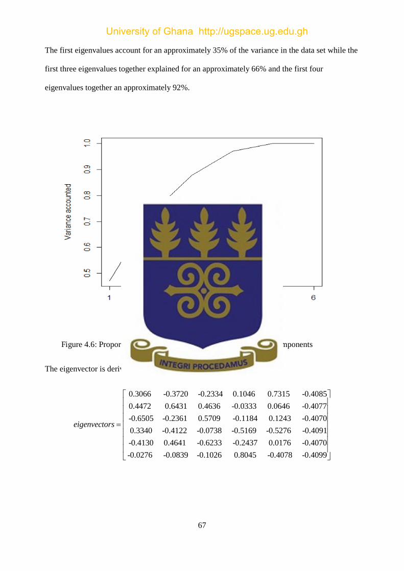
67

The first eigenvalues account for an approximately 35% of the variance in the data set while the

first three eigenvalues together explained for an approximately 66% and the first four

eigenvalues together an approximately 92%.

Figure 4.6: Proportion of the variance explained by the principal components

The eigenvector is derived from cv v where v is the eigenvector:

0.3066 -0.3720 -0.2334 0.1046 0.7315 -0.4085

0.4472 0.6431 0.4636 -0.0333 0.0646 -0.4077

-0.6505 -0.2361 0.5709 -0.1184 0.1243 -0.4070

0.3340 -0.4122 -0.0738 -0.5169 -0.5276 -0.4091

-0.4130 0.4641 -0.6

eigenvectors

233 -0.2437 0.0176 -0.4070

-0.0276 -0.0839 -0.1026 0.8045 -0.4078 -0.4099


68

Step Eight: Eigenface

The eigenfaces are computed as;

Eigen Face= Eigen vector mean centered

Plate 4.4 shows the eigenfaces corresponding to the six train images

Plate 4.4: Image of the eigenface of the trained image

Step Nine: (Principal Component Analysis)

The principal component of the trained is given as

Faces (Γ) =Eigenface mean centered

-160.3687 -242.0858 335.1241 -170.9149 223.9642 14.2811

136.4290 -238.6740 88.7261 152.3101 -169.0179 30.2267

-63.7019 140.9452 158.3819 -18.7857 -184.9114 -31.9281

23.8370 -4.1111 -26.2442 -114.2033 -58.2758 178faces

.9974

93.4786 10.7522 14.2499 -66.5693 -0.3244 -51.5870

0.0000 -0.0000 -0.0000 -0.0000 -0.0000 0.0000

Image of the principal component display of the trained image


69

Figure 4.6 Image of principal component

Again, their brightness is tagged directly to their level of importance in describing the variability

in the image. This means high level of brightness corresponds to high variability and therefore

high importance of that point in carrying information about the image characteristics.

4.2.3 Recognition Procedure Stage

This stage accounts for a step by step approach to recognizing an unknown face in the trained

database.

Recall equation (3.59), the recognition was determined.

4.2.4 Recognition (Euclidean) Distance

The recognition (euclidean) distance for the various angular pose from their straight position is

display in the Table (4.1).


70

Table 4.1: The euclidean distance for the ten image in the train dataset.

4 8 12 16 20 24 28 32

10.405 16.209 21.806 27.581 32.392 36.737 39.489 38.596

11.134 10.727 15.062 21.341 28.049 36.304 44.245 51.687

7.5496 9.4757 12.376 16.377 21.669 27.687 34.071 40.492

9.6804 13.774 17.912 22.623 25.976 28.416 30.41 32.614

4.3542 8.3438 12.55 16.485 20.331 24.798 29.166 33.122

6.9719 12.342 18.608 24.375 30.413 35.756 38.254 37.399

8.3455 13.808 20.139 27.335 34.3 40.567 45.087 46.734

10.03 16.551 22.694 28.339 33.091 34.614 32.337 30.516

7.3898 11.584 18.223 26.311 35.853 45.343 52.993 59.356

7.8737 7.2926 15.341 24.917 35.449 46.21 56.213 61.881

Source: Matlab Output

From Table (4.1), it is obvious that as an individual increase the angular position of the head pose

as the recognition (euclidean) distance increases.

4.3 Statistical Evaluation of the Euclidean Distance

The face recognition algorithms under study is the DWT-PCA/SVD with a Gaussian filter. To

assess whether significant difference exist between the various angular pose from the straight,

repeated measures design was adopted. This statistical technique requires the study dataset to be

multivariate normality distributed.

4.3.1 Assessing for Normality

Normality test is a juxtapose assumption to identify a particular distribution. Since the dataset has

multiple angular pose, the study investigate to identify whether the euclidean distance from the

train image follow a parametric distribution or non-parametric distribution.


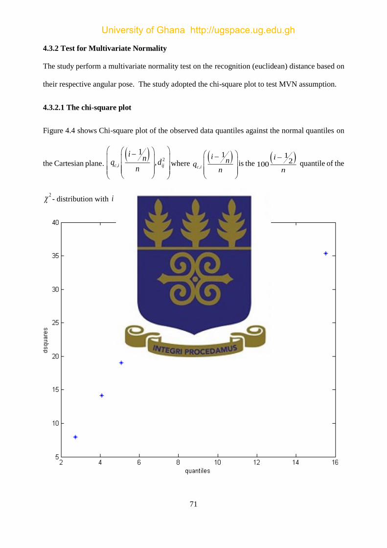
71

4.3.2 Test for Multivariate Normality

The study perform a multivariate normality test on the recognition (euclidean) distance based on

their respective angular pose. The study adopted the chi-square plot to test MVN assumption.

4.3.2.1 The chi-square plot

Figure 4.4 shows Chi-square plot of the observed data quantiles against the normal quantiles on

the Cartesian plane.

2

,

1

,c i ij

in

q dn

where

,

1

c i

in

qn

is the 1

2100

i

n

quantile of the

2 - distribution with i degree freedom.


72

Figure 4.4: A graph of observed data quantiles against the normal quantiles

It can be seen from Figure 4.4 that, the graph consistently deviates from the unit slope. Also using

the correlation test, the correlation, r, value between the observed data quantiles and the normal

quantiles is 0.8386. This value (0.8386) is less than the expected 0.9198 for a sample size of n =

10 and a significance level of 5%. It can therefore be concluded that the assumption of

multivariate normality is not tenable at 5% level of significance. It should however be noted that

there is no absolutely definitive method for testing multivariate normality.

The non-parametric counterpart (Friedman Rank Sum Test) is explored as a substitute for the

repeated measure design.

4.3.3 Friedman Rank Sum Test

The Friedman test was used to evaluate median differences among the angular frontal pose of the

trained image. The results are displayed in the Table (4.3).

Table 4.3: Friedman Test

Friedman Rank Sum Test

chi-square DF P-Value

6.6367 7 7.99E-12

Source: R output

The result from Table (4.3) reject the null hypothesis and states that there is enough evidence to

support the claim that there exist significant difference in the median euclidean distances among

the angular pose (2 6.6367R ; p-value 127.99 10 ). The study further did a pairwise

comparison to investigate which angular pose position causes a significant difference in the

median recognition (euclidean) distance.

The results of the pairwise comparison (Friedman Rank Sum test) is shown in Table (4.4) which

revealed that at 5% level of significance, the pair angular position at 4 , 20 , 4 , 24 ,


73

4 , 28 and 4 ,32 ; angular position pose at 8 ,24 , 8 ,28 and 8 ,32 ; angular

position pose at 12 ,28 and 12 ,32 ; angular position pose at 16 ,32 are statistical

significantly different in median recognition distance.

It can therefore be concluded that recognition distances of head-poses 4 and 8 are significantly

lower than those of head-poses 20 and above, when these constraints are being recognised by

the study algorithm. Recognition distances of head-pose 12 is significantly lower that those of

head-poses 28 and above, when these constraints are being recognised by the study algorithm

whereas recognition distances for head-pose 16 is significantly lower than that head-pose 32 ,

when these constraints are being recognised by the study algorithm. It can be inferred from

submission below that, the higher the degrees of head-pose the larger the recognition distances

and that at 20 and above, the recognition distances become profoundly larger compared to the

4 head pose.

Table 4.4: Pairwise comparisons (Post hoc of the Friedman Test)

4 8 12 16 20 24 28

8 0.99939 - - - - - -

12 0.7239 0.95797 - - - - -

16 0.1723 0.47609 0.98494 - - - -

20 0.00635* 0.04024* 0.47609 0.95797 - - -

24 0.00014* 0.00152* 0.06841** 0.47609 0.98494 - -

28 2.00E-06* 3.60E-05* 0.00451* 0.0877** 0.66454 0.99196 -

32 2.50E-07* 5.40E-06* 0.00104* 0.03036* 0.41504 0.93595 0.99996 * implies significance difference exist between angular constraints at 5% significance level

** implies significance difference exist between angular constraints at 10% significance level

4.3.4 Recognition Rate

The Massachusetts Institute Technology (MIT) database is used to test the performance of the

recognition rate adopting the modify DWT-PCA/SVD under angular constraints.


74

Recall, equation (3.51), the total number of correct recognition 20

1

70q

j

cls

j

n

for algorithm, the

total number of experimental runs 20q and the total number of face images in a single

experimental runs 4totn .

The average (mean) recognition rate of the face algorithm is

70

100 87.5%20 4

avgR

The average error rate of the face algorithm is

100 87.5 12.5%avgE

The average runtime of the face algorithm in the recognition of the 80 face images is

approximately 4 seconds.

Table 4.5: Recognition Rate

4 8 12 16 20 24 28 32

100% 100% 100% 100% 100% 90% 60% 50%

Source: R output

With reference to Table (4.5), there is an evidence that the modify DWT-PCA/SVD algorithm

recognition rate obtained an 100% precision for the angular constraints 4 ,8 ,12 ,16 and 20

but decline steeply for all angular constraints that exceed 20 .

4.3.5 Recognition Curve

The study displayed the graphical representation of the recognition rate with respect to the angular

pose.


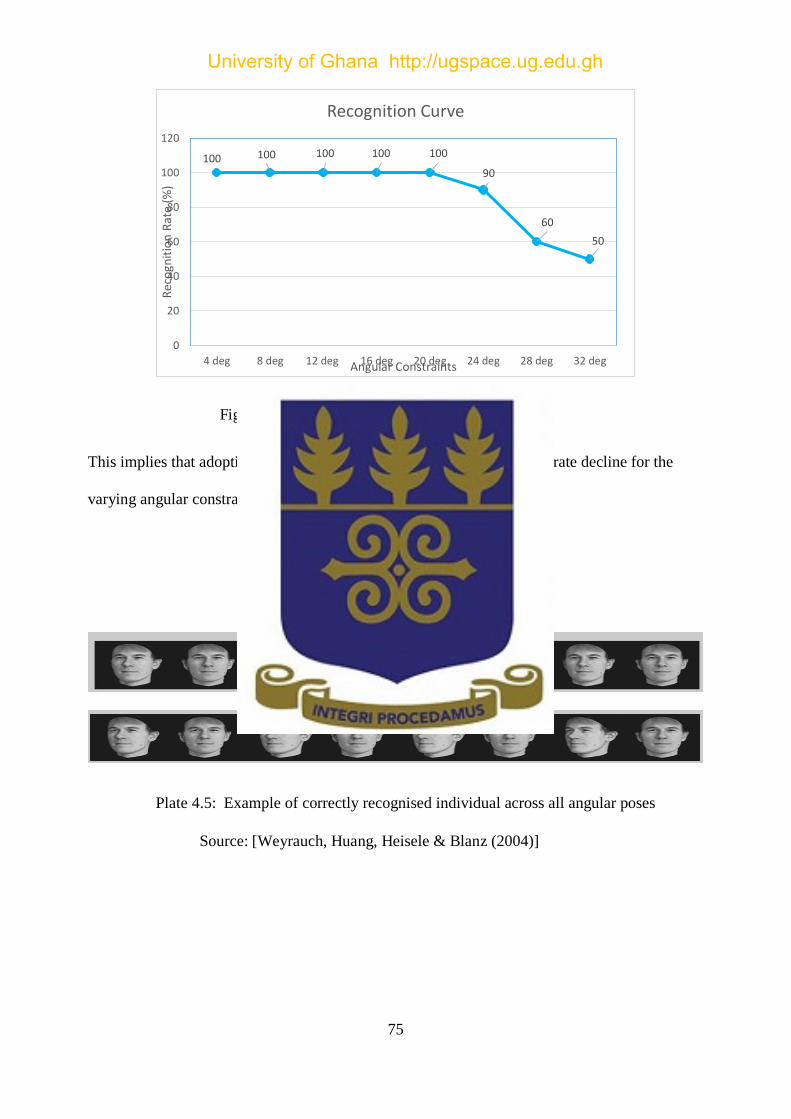
75

Figure 4.5: Displayed the recognition curve

This implies that adopting a DWT-PCA/SVD algorithm, the recognition rate decline for the

varying angular constraint above 20 .

Plate 4.5: Example of correctly recognised individual across all angular poses


100 100 100 100 100

90

60

50

0

20

40

60

80

100

120

4 deg 8 deg 12 deg 16 deg 20 deg 24 deg 28 deg 32 deg

Rec

ogn

itio

n R

ate

(%)

Angular Constraints

Recognition Curve


76

CHAPTER FIVE

Summary, Conclusion and Recommendation

5.1 Introduction

This is the final chapter of the study and also makes recommendations for future thesis work to

be done in this field.

5.2 Summary

The study provided a concrete application of face recognition algorithm using Discrete Wavelet

Transform and Principal Component Analysis with Singular Value Decomposition (DWT-

PCA/SVD) under angular constraint. The study used ten images with an angular constraint from

Massachusetts Institute of Technology database (2002-2005).

From the numerical evaluations in the previous chapter, the recognition rates of Principal

Component Analysis with Singular Value Decomposition (PCA/SVD) with Discrete Wavelet

Transform as a noise removal technique in preprocessing stage (DWT-PCA/SVD) is 87.5% and

a mean error rate is 12.5%.

The average runtime of the modify DWT-PCA/SVD algorithm in the recognition of the 80 face

images in the dataset is approximately 4 seconds. The time used by DWT-PCA/SVD algorithm

in preprocessing accounts for the algorithm’s runtime (speed).

It can be concluded from the results of the Friedman Rank Sum test design that, statistically there

exist statistical significance difference in the recognition distances between the varying angular

constraints o o o o o o o o4 ,8 ,12 ,16 ,20 ,24 ,28 and 32 and their straight-pose 0 . The post hoc

revealed that median euclidean distance for the angular pose position, there exists a significance

difference whenever the angular position are far apart.


77

5.3 Conclusions and Recommendations

The study successfully modified the Principal Component Analysis and Singular Value

Decomposition (PCA/SVD) algorithm by using Discrete Wavelet Transform as noise removal

mechanisms during the face image pre-processing stage.

Adopting the study numerical evaluation, it can be concluded that, DWT-PCA/SVD has an

appreciable performance when used to recognise face images under angular constraints.

A non-parametric statistical technique (Friedman Rank Sum test) has been used to assess whether

statistical significant difference exist between the mean recognition distances of the varying

angular head pose and their straight pose when recognised by DWT-PCA/SVD. From the study

finding, it is highly probable that the face images captured with angular constraints less than or

equal to 20 can be recognise by the study algorithm (DWT-PCA/SVD). Discrete Wavelet

Transform is therefore suggested as a feasible de-noise technique, which ought to be employed

throughout pre-processing stages in image processing.

Future studies should be carried out to analyse the effect of other noise removal mechanism.

Another area for future research could be a study on other constraints like, ageing, occlusions,

face images in glasses and lightening conditions.


78

REFERENCE

Abdullah, M., Wazzan, M., & Bo-Saeed, S. (2012). Optimizing face recognition using pca. arXiv

preprint arXiv:1206.1515.

Asiedu, L., Adebanji, A. O., Oduro, F., & Mettle, F. O. (2015). Statistical evaluation of face

recognition techniques under variable environmental constraints. International Journal of

Statistics and Probability, 4(4), 93.

Baah, G. S. (2013). Face Recognition Using Principal Component Analysis. Knustspace.

Barnouti, N. H., Al-Dabbagh, S. S. M., Matti, W. E., & Naser, M. A. S. (2016). Face Detection

and Recognition Using Viola-Jones with PCA-LDA and Square Euclidean Distance.

International Journal of Advanced Computer Science and Applications (IJACSA), 7(5).

Bartlett, M. S., Movellan, J. R., & Sejnowski, T. J. (2002). Face recognition by independent

component analysis. IEEE Transactions on neural networks, 13(6), 1450-1464.

Beham, M. P., & Roomi, S. M. M. (2012). Face recognition using appearance based approach:

A literature survey. Paper presented at the Proceedings of International Conference &

Workshop on Recent Trends in Technology, Mumbai, Maharashtra, India.

Belhumeur, P. N., Jacobs, D. W., Kriegman, D. J., & Kumar, N. (2013). Localizing parts of faces

using a consensus of exemplars. IEEE Transactions on pattern analysis and machine

intelligence, 35(12), 2930-2940.

Bellakhdhar, F., Loukil, K., & Abid, M. (2013). Face recognition approach using Gabor

Wavelets, PCA and SVM. International Journal of Computer Science Issues, 10(2), 201-

207.

Bhattacharyya, S. K., & Rahul, K. (2013). Face recognition by linear discriminant analysis.

International Journal of Communication Network Security, 2(2), 31-35.

Bledsoe, W. (1964). The model method in facial recognition, Panoramic Research Inc., Palo Alto:

CA, Technical Report, Technical Report PRI: 15.


79

Brunelli, R., & Poggio, T. (1993). Face recognition: Features versus templates. IEEE

Transactions on pattern analysis and machine intelligence, 15(10), 1042-1052.

Bruner, J. S., & Tagiuri, R. (1954). The perception of people. In" Handbook of Social Psychology,

vol. II.(Lindzey, G., ed.): Cambridge, Mass: Addison-Wesley.

Bultheel, A. (1995). Learning to swim in a sea of wavelets. Bulletin of the Belgian Mathematical

society-simon stevin, 2(1), 1-45.

Chang, S. G., Yu, B., & Vetterli, M. (2000). Adaptive wavelet thresholding for image denoising

and compression. IEEE transactions on image processing, 9(9), 1532-1546.

Chellappa, R., Wilson, C. L., & Sirohey, S. (1995). Human and machine recognition of faces: A

survey. Proceedings of the IEEE, 83(5), 705-741.

Darwin, C. (1872). The expression of the emotions in man and animals John Murray: London.

Daubechies, I., Mallat, S., & Willsky, A. S. (1992). Special issue on wavelet transforms and

multiresolution signal analysis-introduction: IEEE-INST ELECTRICAL

ELECTRONICS ENGINEERS INC 345 E 47TH ST, NEW YORK, NY 10017-2394.

De Carrera, P. F., & Marques, I. (2010). Face recognition algorithms. Master's thesis in Computer

Science, Universidad Euskal Herriko.

Dhoke, P., & Parsai, M. (2014). Amatlab based face recognition using PCA with back

propagation neural network. Int. J. Innov. Res. Comput. Commun. Eng, 2(8).

Draper, B. A., Baek, K., Bartlett, M. S., & Beveridge, J. R. (2003). Recognizing faces with PCA

and ICA. Computer vision and image understanding, 91(1), 115-137.

Galton, F. (1892). Finger prints: Macmillan and Company.

Georghiades, A. S., Belhumeur, P. N., & Kriegman, D. J. (2001). From few to many: Illumination

cone models for face recognition under variable lighting and pose. IEEE Transactions on

pattern analysis and machine intelligence, 23(6), 643-660.


80

Goyal, S., & Batra, N. (2016). Using 3G Dongle, Recognition and Reporting based on Pervasive

Computing. International Journal of Computer Science and Information Security, 14(10),

907.

Gross, R., & Brajovic, V. (2003). An image preprocessing algorithm for illumination invariant

face recognition. Paper presented at the AVBPA.

Guillamet, D., & Vitria, J. (2002). Non-negative matrix factorization for face recognition. CCIA,

2, 336-344.

Harandi, M. T., Ahmadabadi, M. N., & Araabi, B. N. (2009). Optimal local basis: A

reinforcement learning approach for face recognition. International Journal of Computer

Vision, 81(2), 191-204.

Haykin, S. S., Haykin, S. S., Haykin, S. S., & Haykin, S. S. (2009). Neural networks and learning

machines (Vol. 3): Pearson Upper Saddle River, NJ, USA:.

Hyvärinen, A., Karhunen, J., & Oja, E. (2004). Independent component analysis (Vol. 46): John

Wiley & Sons.

Johnson, R. A., & Wichern, D. (1998). Multivariate analysis. Wiley StatsRef: Statistics Reference

Online.

Kabir, M. S., Hossain, M. S., & Islam, R. (2016). PERFORMANCE ANALYSIS BETWEEN

PCA AND ICA IN HUMAN FACE DETECTION.

Kadam, K. D. (2014). Face Recognition using Principal Component Analysis with DCT.

International Journal of Engineering Research and General Science, ISSN, 2091-2730.

Kakade, S. D. (2016). A review paper on face recognition techniques. International Journal for

Research in Engineering Application & Management (IJREAM).

Kanade, T. (1973). Computer Recognition of Human Faces, Birkhauser, Basel, Switzerland and

Stuttgart: Germany.


81

Kelly, M. D. (1970). Visual identification of people by computer: STANFORD UNIV CALIF

DEPT OF COMPUTER SCIENCE.

Kirby, M., & Sirovich, L. (1990). Application of the Karhunen-Loeve procedure for the

characterization of human faces. IEEE Transactions on pattern analysis and machine

intelligence, 12(1), 103-108.

Kociołek, M., Materka, A., Strzelecki, M., & Szczypiński, P. (2001). Discrete wavelet transform-

derived features for digital image texture analysis. Paper presented at the International

Conference on Signals and Electronic Systems.

Kohonen, T. (1989). Self-organization and associative memory (Vol. 8): Springer Science &

Business Media.

Kshirsagar, V., Baviskar, M., & Gaikwad, M. (2011). Face recognition using Eigenfaces. Paper

presented at the Computer Research and Development (ICCRD), 2011 3rd International

Conference on.

Lai, J. H., Yuen, P. C., & Feng, G. C. (2001). Face recognition using holistic Fourier invariant

features. Pattern Recognition, 34(1), 95-109.

Liao, S., Jain, A. K., & Li, S. Z. (2013). Partial face recognition: Alignment-free approach. IEEE

Transactions on pattern analysis and machine intelligence, 35(5), 1193-1205.

Liu, Z., Zhou, J., & Jin, Z. (2010). Face recognition based on illumination adaptive LDA. Paper

presented at the Pattern Recognition (ICPR), 2010 20th International Conference on.

Luo, L., Swamy, M., & Plotkin, E. I. (2003). A modified PCA algorithm for face recognition.

Paper presented at the Electrical and Computer Engineering, 2003. IEEE CCECE 2003.

Canadian Conference on.

Moghaddam, B., & Pentland, A. (1997). Probabilistic visual learning for object representation.

IEEE Transactions on pattern analysis and machine intelligence, 19(7), 696-710.


82

Murtaza, M., Sharif, M., Raza, M., & Shah, J. (2014). Face recognition using adaptive margin

fisher’s criterion and linear discriminant analysis. International Arab Journal of

Information Technology, 11(2), 1-11.

Murugan, D., Arumugam, S., Rajalakshmi, K., & Manish, T. (2010). Performance evaluation of

face recognition using Gabor filter, log Gabor filter and discrete wavelet transform.

International journal of computer science & information Technology (IJCSIT), 2(1).

Nicholl, P., & Amira, A. (2008). DWT/PCA face recognition using automatic coefficient

selection. Paper presented at the Electronic Design, Test and Applications, 2008. DELTA

2008. 4th IEEE International Symposium on.

Passalis, G., Perakis, P., Theoharis, T., & Kakadiaris, I. A. (2011). Using facial symmetry to

handle pose variations in real-world 3D face recognition. IEEE Transactions on pattern

analysis and machine intelligence, 33(10), 1938-1951.

Paul, L. C., & Al Sumam, A. (2012). Face recognition using principal component analysis

method. International Journal of Advanced Research in Computer Engineering &

Technology (IJARCET), 1(9), pp: 135-139.

Poularikas, A. (1999). The Hankel transform. The Handbook of Formulas and Tables for Signal

Processing.

Ramalingam, P., & Dhanushkodi, S. (2016). Recognizing Expression Variant and Occluded Face

Images Based on Nested HMM and Fuzzy Rule Based Approach. Circuits and Systems,

7(06), 983.

Reddy, K. R. L., Babu, G., & Kishore, L. (2011). Face recognition based on eigen features of

multi scaled face components and artificial neural network. International Journal of

Security and Its Applications, 5(3), 23-44.


83

Sahu, G., & Tiwari, A. (2015). Training Free Face Recognition and Cropping using Skin

Identification Algorithm. International Journal of Scientific & Engineering Research,

6(3).

Sahu, K., Singh, Y. P., & Kulshrestha, A. (2013). A Comparative Study of Face Recognition

System Using PCA and LDA. International Journal of IT, Engineering and Applied

Sciences Research, 2(10).

Shan, C., Gong, S., & McOwan, P. W. (2009). Facial expression recognition based on local binary

patterns: A comprehensive study. Image and Vision Computing, 27(6), 803-816.

Singh, A., Singh, S. K., & Tiwari, S. (2012). Comparison of face Recognition Algorithms on

Dummy Faces. The International Journal of Multimedia & Its Applications, 4(4), 121.

Singh, N. A., Kumar, M. B., & Bala, M. C. (2016). Face Recognition System based on SURF and

LDA Technique. International Journal of Intelligent Systems and Applications, 8(2), 13.

Sirovich, L., & Kirby, M. (1987). Low-dimensional procedure for the characterization of human

faces. Josa a, 4(3), 519-524.

Szeliski, R. (2010). Computer vision: algorithms and applications: Springer Science & Business

Media.

Thakur, S., Sing, J. K., Basu, D. K., Nasipuri, M., & Kundu, M. (2008). Face recognition using

principal component analysis and RBF neural networks. Paper presented at the Emerging

Trends in Engineering and Technology, 2008. ICETET'08. First International Conference

on.

Turk, M., & Pentland, A. (1991). Eigenfaces for recognition. Journal of cognitive neuroscience,

3(1), 71-86.

Vijg, J. (2011). The American Technological Challenge: Stagnation and Decline in the 21st

Century: Algora Publishing.


84

Wagner, P. (2012). Face recognition with python. Tersedia dalam: www. bytefish. de [diakses

pada 16 Februari 2015].

Weyrauch, B., Heisele, B., Huang, J., & Blanz, V. (2004). Component-based face recognition

with 3D morphable models. Paper presented at the Computer Vision and Pattern

Recognition Workshop, 2004. CVPRW'04. Conference on.

Woodward Jr, J. D., Horn, C., Gatune, J., & Thomas, A. (2003). Biometrics: A look at facial

recognition: RAND CORP SANTA MONICA CA.


85

APPENDIX I

CODES

Imdata <- read.csv(file.choose(),header = TRUE)

Imdata

attach(Imdata)

names(Imdata)

Imdata <- as.matrix(Imdata)

names(Imdata)

shapiro.test(Imdata[,1])








a=cbind(c(0.0184,-0.0045,-0.0097,0.0052,-0.0090,-0.0005),c(-0.0045,0.0315,-0.0125,-0.0033,-

0.0063,-0.0049),c(-0.0097,-0.0125,0.0331,-0.0080,-0,-0.0028),c(0.0052,-0.0033,-

0.0080,0.0215,-0.010,-0.0055),c(-0.0090,-0.0063,-0,-0.01,0.0289,-0.0035),c(-0.0005,-0.0049,-

0.0028,-0.0055,-0.0035,0.0171))

a

eigen(a, symmetric, only.values = FALSE, EISPACK = FALSE)

Eigenvalues <- eigen(cov(a))

g=sort(Eigenvalues$values)

g


86

attach(g)

q=sort(g, decreasing=TRUE)

q

t=q/sum(q)

t

plot(cumsum(t),type="l",xlab="No. of eigenvalues", ylab="Variance accounted")


87

APPENDIX II

Univariate normal test for varying angular constraints

4 8 12 16 20 24 28 32

0.6684 0.8023 0.628 0.1372 0.2469 0.6082 0.4598 0.2476


88


face recognition under angular constraint using …

Documents