Face Poser: Interactive Modeling of 3D Facial Expressions Using Facial Priors

Manfred Lau1,3 Jinxiang Chai2 Ying-Qing Xu3 Heung-Yeung Shum3

1Carnegie Mellon University 2Texas A&M University 3Microsoft Research Asia

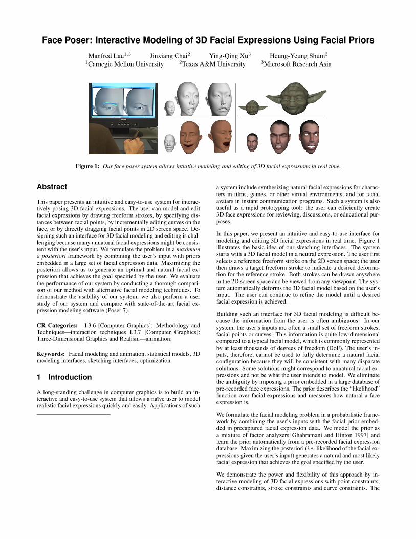
Figure 1: Our face poser system allows intuitive modeling and editing of 3D facial expressions in real time.

Abstract

This paper presents an intuitive and easy-to-use system for interac-tively posing 3D facial expressions. The user can model and editfacial expressions by drawing freeform strokes, by specifying dis-tances between facial points, by incrementally editing curves on theface, or by directly dragging facial points in 2D screen space. De-signing such an interface for 3D facial modeling and editing is chal-lenging because many unnatural facial expressions might be consis-tent with the user’s input. We formulate the problem in a maximuma posteriori framework by combining the user’s input with priorsembedded in a large set of facial expression data. Maximizing theposteriori allows us to generate an optimal and natural facial ex-pression that achieves the goal specified by the user. We evaluatethe performance of our system by conducting a thorough compari-son of our method with alternative facial modeling techniques. Todemonstrate the usability of our system, we also perform a userstudy of our system and compare with state-of-the-art facial ex-pression modeling software (Poser 7).

CR Categories: I.3.6 [Computer Graphics]: Methodology andTechniques—interaction techniques I.3.7 [Computer Graphics]:Three-Dimensional Graphics and Realism—animation;

Keywords: Facial modeling and animation, statistical models, 3Dmodeling interfaces, sketching interfaces, optimization

1 Introduction

A long-standing challenge in computer graphics is to build an in-teractive and easy-to-use system that allows a naıve user to modelrealistic facial expressions quickly and easily. Applications of such

a system include synthesizing natural facial expressions for charac-ters in films, games, or other virtual environments, and for facialavatars in instant communication programs. Such a system is alsouseful as a rapid prototyping tool: the user can efficiently create3D face expressions for reviewing, discussions, or educational pur-poses.

In this paper, we present an intuitive and easy-to-use interface formodeling and editing 3D facial expressions in real time. Figure 1illustrates the basic idea of our sketching interfaces. The systemstarts with a 3D facial model in a neutral expression. The user firstselects a reference freeform stroke on the 2D screen space; the userthen draws a target freeform stroke to indicate a desired deforma-tion for the reference stroke. Both strokes can be drawn anywherein the 2D screen space and be viewed from any viewpoint. The sys-tem automatically deforms the 3D facial model based on the user’sinput. The user can continue to refine the model until a desiredfacial expression is achieved.

Building such an interface for 3D facial modeling is difficult be-cause the information from the user is often ambiguous. In oursystem, the user’s inputs are often a small set of freeform strokes,facial points or curves. This information is quite low-dimensionalcompared to a typical facial model, which is commonly representedby at least thousands of degrees of freedom (DoF). The user’s in-puts, therefore, cannot be used to fully determine a natural facialconfiguration because they will be consistent with many disparatesolutions. Some solutions might correspond to unnatural facial ex-pressions and not be what the user intends to model. We eliminatethe ambiguity by imposing a prior embedded in a large database ofpre-recorded face expressions. The prior describes the “likelihood”function over facial expressions and measures how natural a faceexpression is.

We formulate the facial modeling problem in a probabilistic frame-work by combining the user’s inputs with the facial prior embed-ded in precaptured facial expression data. We model the prior asa mixture of factor analyzers [Ghahramani and Hinton 1997] andlearn the prior automatically from a pre-recorded facial expressiondatabase. Maximizing the posteriori (i.e. likelihood of the facial ex-pressions given the user’s input) generates a natural and most likelyfacial expression that achieves the goal specified by the user.

We demonstrate the power and flexibility of this approach by in-teractive modeling of 3D facial expressions with point constraints,distance constraints, stroke constraints and curve constraints. The

constraints are specified in the 2D screen space. We thereby avoidthe need for complex 3D interactions, which are common in meshediting software and can be cumbersome for a naıve user. We havefound that a first-time user can learn to use the system easily andquickly and be able to create desired facial expressions within min-utes. Figure 1 shows some examples of facial expressions generatedby novices.

We demonstrate potential applications of our system in trajectorykeyframing, face expression transfer between different subjects,and expression posing from photos. We evaluate the quality ofsynthesized facial expressions by comparing against ground truthdata. In addition, we perform a thorough comparison of our methodwith alternative data-driven facial modeling techniques. Finally, weevaluate the usability of our system by performing a user study andcomparing it against Poser 7.

1.1 Contributions

An initial version of our facial modeling framework has appearedpreviously in [Lau et al. 2007]. While this paper uses the same un-derlying probabilistic framework and the point/stroke constraintsdescribed in that paper, this paper is a major improvement overthe original one (approximately half of the material in this paperis new). More specifically, this paper incorporates the followingmajor contributions/improvements over the original one:

• We have added three new constraints (fixed constraints, curveconstraints, and distance constraints) for facial modeling andediting. These constraints were specifically added in responseto comments by the users who previously tested our sys-tem. We show why each of these constraints is important bydemonstrating what each one can do that others cannot. Theseconstraints all together contributes to a usable and completesystem. In addition, they are all designed to fit within a unifiedprobabilistic framework.

• We have conducted a thorough comparison of our methodagainst state-of-the-art facial modeling techniques, includingblendshape interpolation, optimization with blendshapes, op-timization in the PCA subspace, optimization in the PCA sub-space with multivariate Guassian priors, and locally weightedregression. We compared cross validation results for differenttypes of constraints, different numbers of constraints, and dif-ferent error measurements. These results not only evaluate theperformance of our whole system, they also justify our use ofthe MFA model. Such a thorough comparison is also valuableto the whole facial modeling and animation community.

• We have introduced two new applications for our system, in-cluding facial expression transfer between different subjectsand expression posing from photos.

• We have performed a user study to demonstrate the usabil-ity of our method and to compare with state-of-the-art facialmodeling software (Poser 7). In addition, we have tested thesystem on two additional facial models: “Yoda” and “Simon”.

2 Background

In this section, we will discuss related work in sketching interfacesfor 3D object modeling. Because we use prerecorded facial datain our system, we will also review research utilizing examples formodeling.

Our work is inspired by sketch-based systems that interpret theuser’s strokes for creating and editing 3D models [Zeleznik et al.

1996; Igarashi et al. 1999]. Zeleznik and his colleagues [1996] in-troduced a sketch-based interface to create and edit rectilinear ob-jects. Igarashi and his colleagues [1999] developed the first sketch-ing interface to interactively model and edit free-form objects. Re-cently, a number of researchers have explored sketch-based inter-faces for mesh editing [Nealen et al. 2005; Kho and Garland 2005].For example, Nealen and his colleagues [2005] presented a sketch-ing interface for laplacian mesh editing where a user draws refer-ence and target curves on the mesh to specify the mesh deforma-tion. Kho and Garland [2005] demonstrated a similar interface forposing the bodies and limbs of 3D characters. Yang and his col-leagues [2005] presented a 3D modeling system to construct 3Dmodels of particular object classes by matching the points andcurves of a set of given 2D templates to 2D sketches. However,direct application of previous sketch-based modeling techniques infacial expression modeling might not work because facial expres-sion is a fine-grained deformation and even the slightest deviationfrom the truth can be immediately detected.

We present an easy-to-use sketching interface for 3D facial mod-eling and editing. Chang and Jenkins [2006] recently presented asimilar sketching interface for facial modeling. However, their in-terface works only for strokes drawn as lines on the screen. Ourstroke interface is more general, allowing for drawing any line,curve, shape, or region on the screen from any viewpoint. Moreimportantly, our system learns facial priors from a large set of pre-recorded facial expression data and uses them to remove the mod-eling ambiguity.

Our work builds upon the success of example-based facial modelingsystems. Previous systems are often based on weighted combina-tions of examples in the original space [Parke 1972; Lewis et al.2000; Sloan et al. 2001] or eigen-space [Blanz and Vetter 1999;Blanz et al. 2003]. These systems first compute weights from user-specified constraints or image data and then use the weights to lin-early interpolate example data.

Zhang and his colleagues [2004] developed an example-based sys-tem for facial expression editing by interactively dragging pointson the face. Their face model is represented as a linear combina-tion of pre-acquired 3D face scans. Several researchers [Joshi et al.2003; Zhang et al. 2003] also proposed to segment a face modelinto multiple regions and represented each subregion as a convexlinear combination of blend shapes. Recently, Meyer and Ander-son [2007] applied Principle Component Analysis (PCA) to a num-ber of facial deformation examples and used them to select a smallnumber of key points for facial deformation control. Example-based approaches have also been applied to edit skeletal mesh struc-tures. For example, Sumner and Popovic [2005] and Der and hiscolleagues [2006] learned a reduced deformable space from a smallset of example shapes, and used an inverse kinematics approach tooptimize the mesh in a reduced deformable space. Their system al-lows the user to interactively deform a skeletal model by posing justa few vertices. Most recently, Feng and his colleagues [2008] com-bined a deformation regression method based on kernel CanonicalCorrelation Analysis (CCA) and a Poisson-based translation solv-ing technique for easy and fast example-based deformation control.

An alternative way to compute the weights of examples is to re-construct them directly from images or video [Blanz and Vetter1999; Pighin et al. 1999; Blanz et al. 2003]. Blanz and his col-leagues [1999; 2003] built a morphable model from 3D scans viaPrincipal Component Analysis (PCA) [Bishop 1996] and appliedthe morphable model to reconstruct a 3D model from a single im-age. Pighin and his colleagues [1999] demonstrated that they canestimate the weights of 3D morphed face models directly from im-ages or video. Chai and his colleagues presented a real-time vision-based performance interface for facial animation, which transforms

a small set of automatically tracked facial features into realistic fa-cial animation by interpolating the closest examples in a databaseat runtime [Chai et al. 2003].

The main difference between our work and previous example-basedmodeling systems is that we automatically learn a nonlinear prob-abilistic distribution function from a large set of prerecorded facialexpression data. With a collection of locally linear sub-models, ourmodel (mixture of factor analyzers) can efficiently capture a non-linear structure that cannot be modeled by existing linear modelssuch as blendshapes or eigen-shapes. In addition, we formulate thefacial modeling problem in a probabilistic framework by combin-ing the user’s inputs with the priors. This enables us to use a widevariety of intuitive constraints for facial modeling and editing, a ca-pability that has not been demonstrated in previous facial modelingsystems.

A number of researchers have also developed statistical models tosolve the inverse kinematics problem for articulated human char-acters. For example, Grochow and his colleagues [Grochow et al.2004] applied a global nonlinear dimensionality reduction tech-nique to human motion data and used the learned statistical posemodel to compute poses from a small set of user-defined con-straints. GPLVM works well for a small set of example data.However, its performance deteriorates rapidly as the size and het-erogeneity of the database increases. Local statistical models aresufficient if the user provides continuous control signals (the per-formance animation problem). Recently, Chai and his colleaguesconstructed a series of local statistical pose models at runtime andreconstructed full body motion from continuous, low-dimensionalcontrol signals obtained from video cameras [Chai and Hodgins2005]. Online local models are more appropriate for creating an-imations (a sequence of poses) from constraints that are known inadvance, for example, when only the hand position will be con-strained. They are not appropriate for our application because theuser’s input is not predefined and could be enforced at any facialpoints. We significantly extend the idea by constructing a statisti-cal model from a large set of facial expression data and using it forinteractive facial modeling and editing.

3 Overview

The main idea of our approach is that facial priors learned from pre-recorded facial expression data can be used to create natural facialexpressions that match the constraints specified by the user. Thecombination of the facial priors and the user-defined constraintsprovide sufficient information to produce 3D facial expressionswith natural appearances.

3.1 Data Preprocessing

We set up a Vicon motion capture system [Vicon Systems 2007]to record facial movements by attaching 55 reflective markers tothe face of a motion capture subject. We captured the subject per-forming a wide variety of facial actions, including basic facial ex-pressions such as anger, fear, surprise, sadness, joy and disgust, aswell as other common facial actions such as speaking and singing.We scanned the 3D model of the subject and then converted therecorded marker motions into a set of deforming mesh models[Chai et al. 2003]. We translated and rotated each frame of thedata to a default position and orientation because facial expressionmodels should be irrelevant of head poses. We collected data fortwo subjects.

We denote a captured facial example in the database as x ∈ Rd,where x is a long vector stacking the 3D positions of all facial ver-tices and d is three times the number of vertices in a facial model.

Figure 2: System overview.

Let M be the total number of facial examples for each subject.We first use Principal Component Analysis (PCA) [Bishop 1996]to preprocess the captured data and obtain a reduced subspace rep-resentation for x:

x = B·p + x (1)

where the vector p ∈ Rr is a low-dimensional representation of afacial model x ∈ Rd. The matrix B is constructed from the eigen-vectors corresponding to the largest eigenvalues of the covariancematrix of the data, and x is the mean of all the examples. Due tothe large dimensions of x, we perform PCA by an incremental SVDmethod described by Brand [2002].

3.2 Problem Statement

We formulate our facial modeling problem in a maximum a poste-riori (MAP) framework. From Bayes’ theorem, the goal of MAP isto infer the most likely facial model p given the user’s input c:

arg maxp pr(p|c) = arg maxppr(c|p)pr(p)

pr(c)

∝ arg maxp pr(c|p)pr(p)(2)

where pr(c) is a normalizing constant, ensuring that the posterioridistribution on the left-hand side is a valid probability density andintegrates to one.

In our implementation, we minimize the negative log of pr(p|c),yielding the following energy minimization problem for facial ex-pression modeling:

p = arg minp − ln pr(c|p)︸ ︷︷ ︸ + − ln pr(p)︸ ︷︷ ︸Elikelihood Eprior

(3)

where the first term, Elikelihood, is the likelihood term that mea-sures how well a face model p matches the user-specified con-straints c, and the second term, Eprior , is the prior term that de-scribes the prior distribution of the facial expressions. The priorterm is used to constrain the generated facial model to stay close tothe training examples. Maximizing the posteriori produces a natu-ral facial mesh model that achieves the goal specified by the user.

(a) (b)

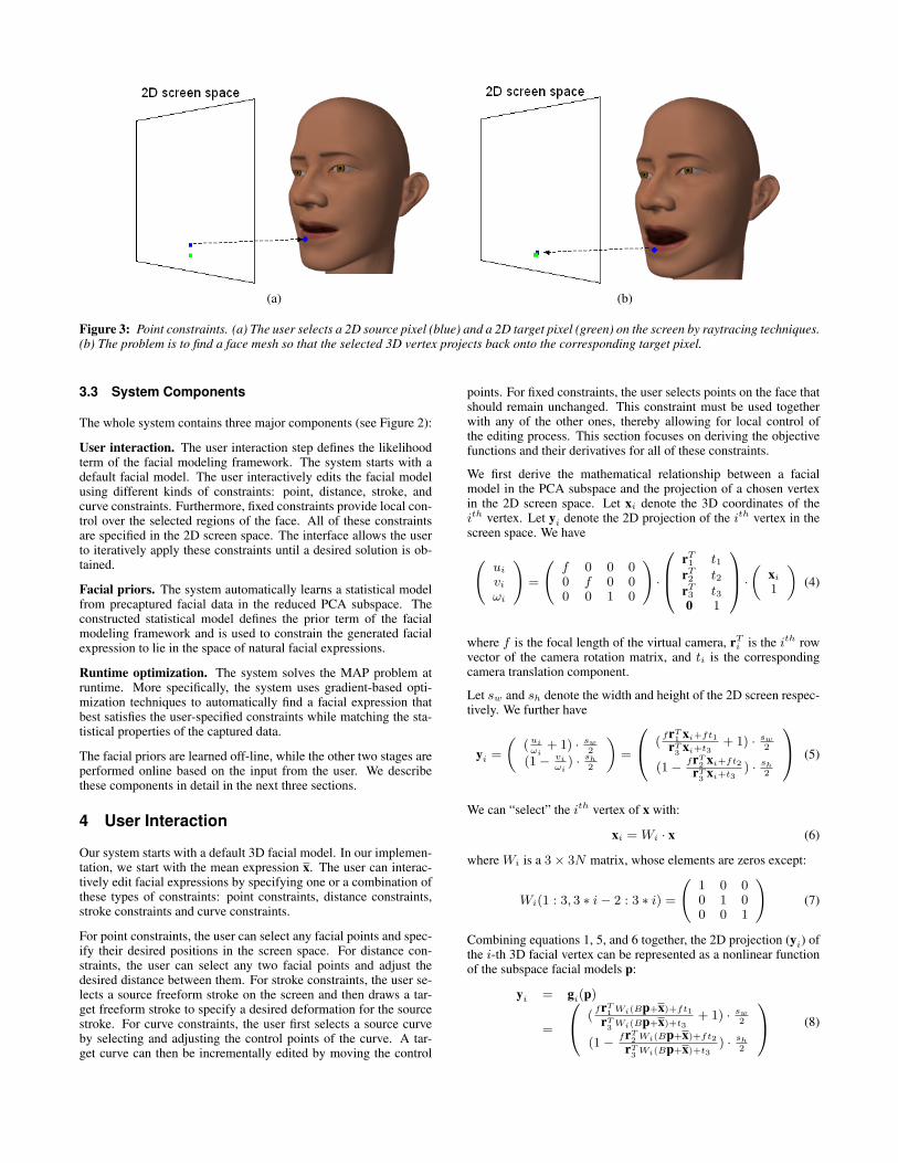
Figure 3: Point constraints. (a) The user selects a 2D source pixel (blue) and a 2D target pixel (green) on the screen by raytracing techniques.(b) The problem is to find a face mesh so that the selected 3D vertex projects back onto the corresponding target pixel.

3.3 System Components

The whole system contains three major components (see Figure 2):

User interaction. The user interaction step defines the likelihoodterm of the facial modeling framework. The system starts with adefault facial model. The user interactively edits the facial modelusing different kinds of constraints: point, distance, stroke, andcurve constraints. Furthermore, fixed constraints provide local con-trol over the selected regions of the face. All of these constraintsare specified in the 2D screen space. The interface allows the userto iteratively apply these constraints until a desired solution is ob-tained.

Facial priors. The system automatically learns a statistical modelfrom precaptured facial data in the reduced PCA subspace. Theconstructed statistical model defines the prior term of the facialmodeling framework and is used to constrain the generated facialexpression to lie in the space of natural facial expressions.

Runtime optimization. The system solves the MAP problem atruntime. More specifically, the system uses gradient-based opti-mization techniques to automatically find a facial expression thatbest satisfies the user-specified constraints while matching the sta-tistical properties of the captured data.

The facial priors are learned off-line, while the other two stages areperformed online based on the input from the user. We describethese components in detail in the next three sections.

4 User Interaction

Our system starts with a default 3D facial model. In our implemen-tation, we start with the mean expression x. The user can interac-tively edit facial expressions by specifying one or a combination ofthese types of constraints: point constraints, distance constraints,stroke constraints and curve constraints.

For point constraints, the user can select any facial points and spec-ify their desired positions in the screen space. For distance con-straints, the user can select any two facial points and adjust thedesired distance between them. For stroke constraints, the user se-lects a source freeform stroke on the screen and then draws a tar-get freeform stroke to specify a desired deformation for the sourcestroke. For curve constraints, the user first selects a source curveby selecting and adjusting the control points of the curve. A tar-get curve can then be incrementally edited by moving the control

points. For fixed constraints, the user selects points on the face thatshould remain unchanged. This constraint must be used togetherwith any of the other ones, thereby allowing for local control ofthe editing process. This section focuses on deriving the objectivefunctions and their derivatives for all of these constraints.

We first derive the mathematical relationship between a facialmodel in the PCA subspace and the projection of a chosen vertexin the 2D screen space. Let xi denote the 3D coordinates of theith vertex. Let yi denote the 2D projection of the ith vertex in thescreen space. We have(

uiviωi

)=

(f 0 0 00 f 0 00 0 1 0

)·

rT1 t1rT2 t2rT3 t30 1

·( xi1

)(4)

where f is the focal length of the virtual camera, rTi is the ith rowvector of the camera rotation matrix, and ti is the correspondingcamera translation component.

Let sw and sh denote the width and height of the 2D screen respec-tively. We further have

yi =

((uiωi

+ 1) · sw2

(1− viωi

) · sh2

)=

(frT

1 xi+ft1

rT3 xi+t3

+ 1) · sw2

(1− frT2 xi+ft2

rT3 xi+t3

) · sh2

(5)

We can “select” the ith vertex of x with:

xi = Wi · x (6)

where Wi is a 3× 3N matrix, whose elements are zeros except:

Wi(1 : 3, 3 ∗ i− 2 : 3 ∗ i) =

(1 0 00 1 00 0 1

)(7)

Combining equations 1, 5, and 6 together, the 2D projection (yi) ofthe i-th 3D facial vertex can be represented as a nonlinear functionof the subspace facial models p:

yi = gi(p)

=

(frT

1 Wi(Bp+x)+ft1

rT3 Wi(Bp+x)+t3

+ 1) · sw2

(1− frT2 Wi(Bp+x)+ft2

rT3 Wi(Bp+x)+t3

) · sh2

(8)

Figure 4: Distance constraints. As input, the user selects pairs ofvertices and specifies the distances between each pair.

4.1 Point Constraints

Point constraints allow the user to change the positions of individ-ual vertices on the mesh. This enables the user to have detailedcontrol over the final result. The user first selects a set of 3D sourcevertices {xi|i = 1, ..., N} and then specifies a corresponding setof 2D target pixels {zi|i = 1, ..., N} of where the vertices shouldmap to on the screen (Figure 3(a)). The user selects each 3D pointby picking a pixel in the 2D screen. We perform ray tracing withthis pixel to choose the point on the mesh. Given these inputs, theproblem is to find a face model so that each selected 3D vertex (xi)projects onto the corresponding 2D screen position (zi) in the cur-rent camera view (Figure 3(b)).

Assuming Gaussian noise with a standard deviation of σpoint forthe i-th point constraint zi, we can define the likelihood term forthe i-th point constraint as follows:

Epoint = − ln pr(zi|p)

= − ln 1√2π

exp−‖yi−zi‖2

σ2point

∝ ‖gi(p)−zi‖2

σ2point

.

(9)

A good match between the generated facial model (p) and the user’sinput (zi) results in a low value for the likelihood term.

4.2 Distance Constraints

This constraint allows the user to select two facial vertices xi andxj , and edit the distance between them in the 2D screen space. Thisis particularly useful for changing the width and height of the eyesor mouth. Figure 4 shows an example of the user’s input. The userselects the 3D vertices by selecting 2D pixels in the same way asthe point constraints. The current distances between the pairs ofvertices are displayed, and the user can dynamically adjust the dis-tances.

Let d denote the user-defined target distance, and let xi and xj mapto yi and yj respectively. Similarly, we assume Gaussian noise witha standard deviation of σdist for the distance constraint d, and wedefine the following likelihood term for the distance constraints:

Edistance = − ln pr(d|p)

= − ln 1√2π

exp−(‖yi−yj‖−d)

2

σ2dist

∝(‖gi(p)−gj(p)‖−d)2

σ2dist

.

(10)

Figure 5: Stroke constraints: different examples of source strokes(blue) and target strokes (green).

Figure 6: If the source and target strokes are originally far awayfrom each other, the objective function in Equation 12 does not al-low the two strokes to “move toward” each other. This motivatesthe need for the additional distance term for stroke constraints.

4.3 Stroke Constraints

This constraint allows the user to select a group of 3D points andspecify where these points should collectively project to on thescreen. This is designed to allow the user to make large-scalechanges to the mesh with minimal user interaction. More specif-ically, the user first draws a 2D source stroke to select a set of 3Dpoints (xs’s) on the mesh. Then the user draws a 2D target stroke toprovide a region of pixels (zj’s) where the 3D points should projectto. Figure 5 shows some examples of user-drawn strokes.

Given a source stroke in the 2D screen space, we need to find thecorresponding 3D points on the mesh efficiently. We ray traced thepixels of the source stroke in a hierarchical manner. We first con-sider the selected pixel region as blocks of 15 by 15 pixels, and findthe triangles that intersect with each block. We then consider theseblocks as 3 by 3 pixels, and find the triangles that intersect witheach block. For each 3 by 3 block, we only test the triangles thatintersected with the corresponding 15 by 15 block. Finally, we raytraced each pixel by testing only the triangles in the corresponding3 by 3 block. This process selects the xs’s on the mesh. This pro-cess is necessary in order to allow for interactive selection of thepoints on the mesh. Without this hierarchical selection, it can takeup to tens of seconds to select the points for each source stroke.

Since the selected 3D points on the mesh do not have to be theoriginal vertices of the mesh, we store the barycentric coordinatesof each xs. The position of each xs depends on the positions of thethree vertices of the triangle (xu, xv , xw) that it belongs to. Whenthe face mesh deforms, the position of each xs is recomputed as:

xs = u · xu + v · xv + w · xw (11)

where u, v, and w are the barycentric coordinates. For a given xs,these barycentric coordinates are fixed, while the vertices (xu, xv ,xw) may deform.

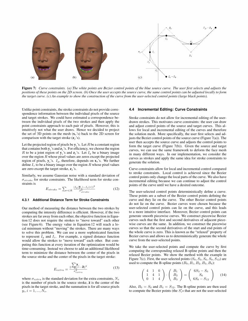
Figure 7: Curve constraints. (a) The white points are Bezier control points of the blue source curve. The user first selects and adjusts thepositions of these points on the 2D screen. (b) Once the user accepts the source curve, the same control points can be adjusted locally to formthe target curve. (c) An example to show the construction of the curve from the user-selected control points (large black points).

Unlike point constraints, the stroke constraints do not provide corre-spondence information between the individual pixels of the sourceand target strokes. We could have estimated a correspondence be-tween the individual pixels of the two strokes and then apply thepoint constraints approach to each pair of pixels. However, this isintuitively not what the user draws. Hence we decided to projectthe set of 3D points on the mesh (xs’s) back to the 2D screen forcomparison with the target stroke (zj’s).

Let the projected region of pixels be yi’s. LetR be a constant regionthat contains both yi’s and zj’s. For efficiency, we choose the regionR to be a joint region of yi’s and zj’s. Let Iy be a binary imageover the region R whose pixel values are zeros except the projectedregion of pixels, yi’s. Iy , therefore, depends on xs’s. We furtherdefine Iz to be a binary image over the regionR whose pixel valuesare zero except the target stroke, zj’s.

Similarly, we assume Gaussian noise with a standard deviation ofσstroke for stroke constraints. The likelihood term for stroke con-straints is

Estroke =∑

r∈R(Iy(yi)−Iz(r))2

σ2stroke

(12)

4.3.1 Additional Distance Term for Stroke Constraints

Our method of measuring the distance between the two strokes bycomputing the intensity difference is efficient. However, if the twostrokes are far away from each other, the objective function in Equa-tion 12 does not require the strokes to “move toward” each other(see Figure 6). The energy value in Equation 12 will reach a lo-cal minimum without “moving” the strokes. There are many waysto solve this problem. We can use a more sophisticated functionto represent Iy and Iz . For example, a signed distance functionwould allow the strokes to “move toward” each other. But com-puting this function at every iteration of the optimization would betime-consuming. Instead we choose to add an additional likelihoodterm to minimize the distance between the center of the pixels inthe source stroke and the center of the pixels in the target stroke:

Eextra =‖

∑yi

Ns−z‖2

σ2extra

(13)

where σextra is the standard deviation for the extra constraints, Nsis the number of pixels in the source stroke, z is the center of thepixels in the target stroke, and the summation is for all source pixelsyi, i = 1, ..., Ns.

4.4 Incremental Editing: Curve Constraints

Stroke constraints do not allow for incremental editing of the user-drawn strokes. This motivates curve constraints: the user can drawand adjust control points of the source and target curves. This al-lows for local and incremental editing of the curves and thereforethe solution mesh. More specifically, the user first selects and ad-justs the Bezier control points of the source curve (Figure 7(a)). Theuser then accepts the source curve and adjusts the control points toform the target curve (Figure 7(b)). Given the source and targetcurves, we can use the same framework to deform the face meshin many different ways. In our implementation, we consider thecurves as strokes and apply the same idea for stroke constraints togenerate the solution.

Curve constraints allow for local and incremental control comparedto stroke constraints. Local control is achieved since the Beziercontrol points only change the local parts of the curve. We also haveincremental editing because we can continue to adjust the controlpoints of the curve until we have a desired outcome.

The user-selected control points deterministically define a curve.These points are a subset of the Bezier control points defining thecurve and they lie on the curve. The other Bezier control pointsdo not lie on the curve. Bezier curves were chosen because theuser-selected control points can lie on the curve, and this leadsto a more intuitive interface. Moreover, Bezier control points cangenerate smooth piecewise curves. We construct piecewise Beziercurves such that the first and second derivatives of adjacent piece-wise curves are the same. In addition, we construct the piecewisecurves so that the second derivatives of the start and end points ofthe whole curve is zero. This is known as the “relaxed” property ofBezier curves and allows us to deterministically generate the wholecurve from the user-selected points.

We take the user-selected points and compute the curve by firstcomputing the corresponding relaxed B-spline points and then therelaxed Bezier points. We show the method with the example inFigure 7(c). First, the user-selected points (S0, S3, S6, S9, S12) areused to compute the B-spline points (B0, B1, B2, B3, B4):(

4 1 01 4 10 1 4

)·

(B1

B2

B3

)=

(6S3 − S0

S6

6S9 − S12

)(14)

Also, B0 = S0 and B4 = S12. The B-spline points are then usedto compute the Bezier points (the S′is that are not the user-selected

(a) (b) (c)

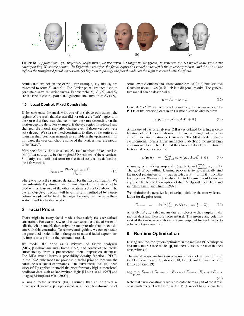
Figure 8: Applications. (a) Trajectory keyframing: we use seven 2D target points (green) to generate the 3D model (blue points arecorresponding 3D source points). (b) Expression transfer: the facial expression model on the left is the source expression, and the one on theright is the transferred facial expression. (c) Expression posing: the facial model on the right is created with the photo.

points) that are not on the curve. For example, B0 and B1 aretri-sected to form S1 and S2. The Bezier points are then used togenerate piecewise Bezier curves. For example, S0, S1, S2, and S3

are the Bezier control points that generate the curve from S0 to S3.

4.5 Local Control: Fixed Constraints

If the user edits the mesh with one of the above constraints, theregions of the mesh that the user did not select are “soft” regions, inthe sense that they may change or stay the same depending on themotion capture data. For example, if the eye region is selected andchanged, the mouth may also change even if those vertices werenot selected. We can use fixed constraints to allow some vertices tomaintain their positions as much as possible in the optimization. Inthis case, the user can choose some of the vertices near the mouthto be “fixed”.

More specifically, the user selectsNF total number of fixed vertices(xi’s). Let xi original be the original 3D positions of these vertices.Similarly, the likelihood term for the fixed constraints defined onthe i-th vertex is

Efixed =‖xi−xi original‖2

σ2fixed

(15)

where σfixed is the standard deviation for the fixed constraints. Wecan substitute Equations 1 and 6 here. Fixed constraints must beused with at least one of the other constraints described above. Theoverall objective function will have this term multiplied by a user-defined weight added to it. The larger the weight is, the more thesevertices will try to stay in place.

5 Facial Priors

There might be many facial models that satisfy the user-definedconstraints. For example, when the user selects one facial vertex toedit the whole model, there might be many results that are consis-tent with this constraint. To remove ambiguities, we can constrainthe generated model to lie in the space of natural facial expressionsby imposing a prior on the generated model.

We model the prior as a mixture of factor analyzers(MFA) [Ghahramani and Hinton 1997] and construct the modelautomatically from a pre-recorded facial expression database.The MFA model learns a probability density function (P.D.F.)in the PCA subspace that provides a facial prior to measure thenaturalness of facial expressions. The MFA model has also beensuccessfully applied to model the prior for many high-dimensionalnonlinear data such as handwritten digits [Hinton et al. 1997] andimages [Bishop and Winn 2000].

A single factor analyzer (FA) assumes that an observed r-dimensional variable p is generated as a linear transformation of

some lower q-dimensional latent variable τ∼N (0, I) plus additiveGaussian noise ω∼N (0,Ψ). Ψ is a diagonal matrix. The genera-tive model can be described as:

p = Aτ + ω + µ (16)

Here,A ∈ Rr×q is a factor loading matrix. µ is a mean vector. TheP.D.F. of the observed data in an FA model can be obtained by:

pr(p; Θ) = N (µ,AAT + Ψ) (17)

A mixture of factor analyzers (MFA) is defined by a linear com-bination of K factor analyzers and can be thought of as a re-duced dimension mixture of Gaussians. The MFA model extractsq-dimensional locally linear manifolds underlying the given highdimensional data. The P.D.F. of the observed data by a mixture offactor analyzers is given by:

pr(p; Θ) =∑K

k=1πkN (µk, AkA

Tk + Ψ) (18)

where πk is a mixing proportion (πk > 0 and∑K

k=1πk = 1).

The goal of our offline learning process is to automatically findthe model parameters Θ = {πk, µk, Ak,Ψ|k = 1, ...,K} from thetraining data. We use an EM algorithm to fit a mixture of factor an-alyzers. The detailed description of the EM algorithm can be foundin [Ghahramani and Hinton 1997].

We minimize the negative log of pr(p), yielding the energy formu-lation for the prior term:

Eprior = − ln∑K

k=1πkN (µk, AkA

Tk + Ψ) (19)

A smaller Eprior value means that p is closer to the samples in themotion data and therefore more natural. The inverse and determi-nant of the covariance matrices are precomputed for each factor toachieve a faster runtime.

6 Runtime Optimization

During runtime, the system optimizes in the reduced PCA subspaceand finds the 3D face model (p) that best satisfies the user-definedconstraints (c).

The overall objective function is a combination of various forms ofthe likelihood terms (Equations 9, 10, 12, 13, and 15) and the priorterm (Equation 19):

arg minp∈Rr

Epoint+Edistance+Estroke+Eextra+Efixed+Eprior

(20)Note that curve constraints are represented here as part of the strokeconstraints term. Each factor in the MFA model has a mean face

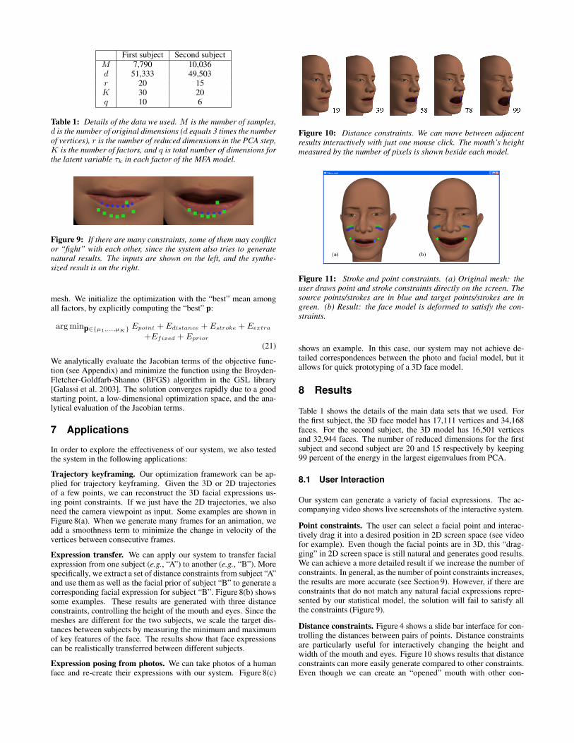
First subject Second subjectM 7,790 10,036d 51,333 49,503r 20 15K 30 20q 10 6

Table 1: Details of the data we used. M is the number of samples,d is the number of original dimensions (d equals 3 times the numberof vertices), r is the number of reduced dimensions in the PCA step,K is the number of factors, and q is total number of dimensions forthe latent variable τk in each factor of the MFA model.

Figure 9: If there are many constraints, some of them may conflictor “fight” with each other, since the system also tries to generatenatural results. The inputs are shown on the left, and the synthe-sized result is on the right.

mesh. We initialize the optimization with the “best” mean amongall factors, by explicitly computing the “best” p:

arg minp∈{µ1,...,µK} Epoint + Edistance + Estroke + Eextra+Efixed + Eprior

(21)

We analytically evaluate the Jacobian terms of the objective func-tion (see Appendix) and minimize the function using the Broyden-Fletcher-Goldfarb-Shanno (BFGS) algorithm in the GSL library[Galassi et al. 2003]. The solution converges rapidly due to a goodstarting point, a low-dimensional optimization space, and the ana-lytical evaluation of the Jacobian terms.

7 Applications

In order to explore the effectiveness of our system, we also testedthe system in the following applications:

Trajectory keyframing. Our optimization framework can be ap-plied for trajectory keyframing. Given the 3D or 2D trajectoriesof a few points, we can reconstruct the 3D facial expressions us-ing point constraints. If we just have the 2D trajectories, we alsoneed the camera viewpoint as input. Some examples are shown inFigure 8(a). When we generate many frames for an animation, weadd a smoothness term to minimize the change in velocity of thevertices between consecutive frames.

Expression transfer. We can apply our system to transfer facialexpression from one subject (e.g., “A”) to another (e.g., “B”). Morespecifically, we extract a set of distance constraints from subject “A”and use them as well as the facial prior of subject “B” to generate acorresponding facial expression for subject “B”. Figure 8(b) showssome examples. These results are generated with three distanceconstraints, controlling the height of the mouth and eyes. Since themeshes are different for the two subjects, we scale the target dis-tances between subjects by measuring the minimum and maximumof key features of the face. The results show that face expressionscan be realistically transferred between different subjects.

Expression posing from photos. We can take photos of a humanface and re-create their expressions with our system. Figure 8(c)

Figure 10: Distance constraints. We can move between adjacentresults interactively with just one mouse click. The mouth’s heightmeasured by the number of pixels is shown beside each model.

Figure 11: Stroke and point constraints. (a) Original mesh: theuser draws point and stroke constraints directly on the screen. Thesource points/strokes are in blue and target points/strokes are ingreen. (b) Result: the face model is deformed to satisfy the con-straints.

shows an example. In this case, our system may not achieve de-tailed correspondences between the photo and facial model, but itallows for quick prototyping of a 3D face model.

8 Results

Table 1 shows the details of the main data sets that we used. Forthe first subject, the 3D face model has 17,111 vertices and 34,168faces. For the second subject, the 3D model has 16,501 verticesand 32,944 faces. The number of reduced dimensions for the firstsubject and second subject are 20 and 15 respectively by keeping99 percent of the energy in the largest eigenvalues from PCA.

8.1 User Interaction

Our system can generate a variety of facial expressions. The ac-companying video shows live screenshots of the interactive system.

Point constraints. The user can select a facial point and interac-tively drag it into a desired position in 2D screen space (see videofor example). Even though the facial points are in 3D, this “drag-ging” in 2D screen space is still natural and generates good results.We can achieve a more detailed result if we increase the number ofconstraints. In general, as the number of point constraints increases,the results are more accurate (see Section 9). However, if there areconstraints that do not match any natural facial expressions repre-sented by our statistical model, the solution will fail to satisfy allthe constraints (Figure 9).

Distance constraints. Figure 4 shows a slide bar interface for con-trolling the distances between pairs of points. Distance constraintsare particularly useful for interactively changing the height andwidth of the mouth and eyes. Figure 10 shows results that distanceconstraints can more easily generate compared to other constraints.Even though we can create an “opened” mouth with other con-

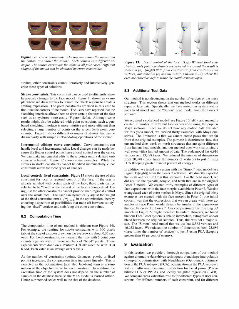
Figure 12: Curve constraints. The top row shows the inputs andthe bottom row shows the results. Each column is a different ex-ample. The source curves are the same in all four cases. Differentshapes of the mouth can be obtained by curve constraints.

straints, other constraints cannot iteratively and interactively gen-erate these types of solutions.

Stroke constraints. This constraint can be used to efficiently makelarge-scale changes to the face model. Figure 11 shows an exam-ple where we draw strokes to “raise” the cheek regions to create asmiling expression. The point constraints are used in this case tofine-tune the corners of the mouth. The users have reported that thesketching interface allows them to draw certain features of the facesuch as an eyebrow more easily (Figure 1(left)). Although someresults might also be achieved with point constraints, such a pen-based sketching interface is more intuitive and more efficient thanselecting a large number of points on the screen (with point con-straints). Figure 5 shows different examples of strokes that can bedrawn easily with simple click-and-drag operations of the mouse.

Incremental editing: curve constraints. Curve constraints canhandle local and incremental edits. Local changes can be made be-cause the Bezier control points have a local control over the curve.We can make incremental edits to these points until a desired out-come is achieved. Figure 12 shows some examples. While thestrokes in stroke constraints cannot be edited incrementally, curveconstraints allow for these types of changes.

Local control: fixed constraints. Figure 13 shows the use of thisconstraint for local or regional control of the face. If the user isalready satisfied with certain parts of the face, those parts can beselected to be “fixed” while the rest of the face is being edited. Us-ing just the other constraints cannot provide such regional controlover the whole face. The user can dynamically adjust the weightof the fixed constraint term (1/σ2

fixed) in the optimization, therebychoosing a spectrum of possibilities that trade off between satisfy-ing the “fixed” vertices and satisfying the other constraints.

8.2 Computation Time

The computation time of our method is efficient (see Figure 14).For example, the runtime for stroke constraints with 900 pixels(about the size of a stroke drawn on the eyebrow) is about 0.35 sec-onds. For fixed constraints, we measure the time with 5 point con-straints together with different numbers of “fixed” points. Theseexperiments were done on a Pentium 4 3GHz machine with 1GBRAM. Each value is an average over 5 trials.

As the number of constraints (points, distances, pixels, or fixedpoints) increases, the computation time increases linearly. This isexpected as the optimization (and also Jacobian) term is a sum-mation of the objective value for each constraint. In addition, theexecution time of the system does not depend on the number ofsamples in the database because the MFA model is learned offline.Hence our method scales well to the size of the database.

Figure 13: Local control of the face. (Left) Without fixed con-straints: only point constraints are selected in (a) and the result isshown in (b). (Right) With fixed constraints: fixed constraint (redvertices) are added in (c) and the result is shown in (d), where theeyes are closed as before while the mouth remains open.

8.3 Additional Test Data

Our method is not dependent on the number of vertices or the meshstructure. This section shows that our method works on differenttypes of face data. Specifically, we have tested our system with ayoda head model and the “Simon” head model from the Poser 7software.

We acquired a yoda head model (see Figure 15(left)), and manuallycreated a number of different face expressions using the popularMaya software. Since we do not have any motion data availablefor this yoda model, we created thirty examples with Maya our-selves. The limitation is that we cannot create poses that are farfrom these original examples. The purpose is therefore to show thatour method does work on mesh structures that are quite differentfrom human head models, and our method does work surprisinglywell even with a limited amount of data. The yoda model has 6,916vertices and 13,788 faces. We reduced the number of dimensionsfrom 20,748 (three times the number of vertices) to just 5 usingPCA (keeping greater than 98 percent of energy).

In addition, we tested our system with the “Simon” head model (seeFigure 15(right)) from the Poser 7 software. We directly exportedthe mesh and texture from this software. For the head model, wedid not use the eyeballs, tongue, and teeth that are in the originalPoser 7 model. We created thirty examples of different types offace expressions with the face morphs available in Poser 7. We alsotriangulated each of these meshes in Maya. Since the original thirtyexamples are created with the face morphs in Poser 7, one initialconcern was that the expressions that we can create with these ex-amples in Face Poser would already be similar to the expressionsthat can be created in Poser 7. Our comparison of the resulting 3Dmodels in Figure 22 might therefore be unfair. However, we foundthat our Face Poser system is able to interpolate, extrapolate and/orblend between the original samples. Thus, this was not a major is-sue. The “Simon” head model that we use has 8,562 vertices and16,952 faces. We reduced the number of dimensions from 25,686(three times the number of vertices) to just 5 using PCA (keepinggreater than 99 percent of energy).

9 Evaluation

In this section, we provide a thorough comparison of our methodagainst alternative data-driven techniques: blendshape interpolation(Interp-all), optimization with blendshapes (Opt-blend), optimiza-tion in the PCA subspace (PCA), optimization in the PCA subspacewith a multivariate Gaussian distribution for facial priors (Proba-bilistic PCA or PPCA), and locally weighted regression (LWR).We compare cross validation results for different types of user con-straints, for different numbers of each constraint, and for different

Runtime for Point Constraints

0

50

100

150

200

250

300

0 5 10 15 20

number of points

time

(ms)

Runtime for Distance Constraints

0

50

100

150

200

250

300

350

400

0 5 10 15 20

number of distances

time

(ms)

Runtime for Stroke Constraints

0

50

100

150

200

250

300

350

400

450

0 200 400 600 800 1000 1200

number of pixels in source or target stroke

time

(ms)

Runtime for Fixed Constraints

0

50

100

150

200

250

300

0 5 10 15 20

number of fixed pointstim

e (m

s)

Figure 14: Computation time for each constraint. As the number of constraints increases, the computation time increases linearly.

Figure 15: These results show that our method works on a variety of face data. (Left) We can edit a 3D yoda model by sketching on the 2Dscreen. (Right) Our system works with the “Simon” head model from the Poser 7 software.

error measurements.

9.1 Explanation of Other Techniques, Cross Valida-tion, 3D and 2D Error

We compare the MFA model used in this work against other meth-ods. The alternative techniques can be classified into two groups:

Interpolation. “Interp-all” takes all the examples in the database,uses the objective function (i.e. Equation 9 for point constraints) tocompute an appropriate weight for each example, and blends the ex-amples with the computed weights [Parke 1972; Lewis et al. 2000;Sloan et al. 2001]. “LWR” extends the idea of “Interp-all” by con-sidering closest examples in the database [Chai et al. 2003]. It findsk examples that are closest to the user’s input and performs a locallyweighted regression based on the closest examples.

Optimization. “Opt-blend” represents the solution as a weighted

combination of examples in the database and optimizes the weightsbased on user-defined constraints [Zhang et al. 2004]. “PCA” sig-nificantly reduces the solution space of “opt-blend” by performingan optimization in the PCA subspace [Blanz and Vetter 1999; Blanzet al. 2003]. “PPCA” further reduces the solution space by incorpo-rating a “Gaussian” prior term into the objective function. “PPCA”assumes that the examples in the database are represented by a mul-tivariate Gaussian distribution. All optimization methods start withthe same initial pose.

For cross validation tests, we use new face models as testing data.We start from a neutral pose and select the source constraints(points, distances, strokes). The corresponding target constraintsare automatically generated based on the ground truth test data. Forexample, if 3D point x is chosen and it maps to the 2D pixel y forthe test data, y is used as the target constraint for the original neutralpose. Given the source and target, we can then generate the solutionand compare it against the ground truth data (i.e. the test data).

Comparison of Techniques - Point Constraints

0.06

0.08

0.10

0.12

0.14

0.16

0.18

0.20

0 2 4 6 8

number of point constraints

3D e

rror

(fro

m c

ross

val

idat

ion)

Opt-blendInterp-allPPCAPCALWRMFA (our method)

Comparison of Techniques - Point Constraints

0

20

40

60

80

100

120

140

0 2 4 6 8

number of point constraints

2D e

rror

Opt-blendInterp-allPPCAPCALWRMFA (our method)

Comparison of Techniques - Distance Constraints

0.13

0.14

0.15

0.16

0.17

0 2 4 6 8

number of distance constraints

3D e

rror

(fro

m c

ross

val

idat

ion)

Opt-blendInterp-allPPCAPCALWRMFA (our method)

Comparison of Techniques - Distance Constraints

0

10

20

30

40

0 2 4 6 8

number of distance constraints

2D e

rror

Opt-blendInterp-allPPCAPCALWRMFA (our method)

Comparison of Techniques - Stroke Constraints

0.13

0.14

0.15

0.16

0.17

0.18

0 100 200 300 400 500

number of pixels

3D e

rror

(fro

m c

ross

val

idat

ion)

Opt-blendInterp-allPPCAPCALWRMFA (our method)

Comparison of Techniques - Stroke Constraints

0.60

0.65

0.70

0.75

0.80

0.85

0.90

0 100 200 300 400 500

number of pixels

2D e

rror

(nor

mal

ized

) Opt-blendInterp-allPPCAPCALWRMFA (our method)

Figure 16: Comparison with other techniques. (Top) Point constraints. (Middle) Distance constraints. (Bottom) Stroke constraints. Figuresin the left and right show 3D and 2D errors respectively.

The 3D error is the average of the Euclidean distances between eachvertex of the ground truth mesh and the synthesized mesh. Forpoint constraints, the 2D error is the difference between the pro-jected pixel (from the selected source vertex) and the target pixel.If there is more than one pair of source vertices and target pixels,we average these differences. This is essentially Equation 9 with pbeing the solution mesh. The 2D error for the other constraints arecomputed similarly by their respective optimization objective func-tions. Each value reported for 3D error, 2D error, and runtime is anaverage over 10 trials.

9.2 Comparison of 3D Reconstruction Error

The left side of Figure 16 show the comparison results of 3D errorsfor point, distance, and stroke constraints respectively. As the num-ber of constraints increases (in all cases), the 3D error decreases.This is because the increase in the number of constraints providesmore information about the ground truth sample. This leads to amore accurate result in the solution mesh compared to the groundtruth, and therefore the 3D error decreases.

“Opt-blend” and “Interp-all” do not produce good results becausethe solution depends on all the samples in the database. PCA pro-duces a larger error because the number of user specified constraintsis usually small even when compared to the reduced dimensions ofthe PCA subspace. Hence the constraints are not sufficient to fullydetermine the weights of p. PPCA can remove the mapping am-biguity from the low-dimensional constraints to the reduced sub-space dimensions by the facial prior. However, the face models arenot as well approximated by a multivariate Gaussian distribution.For LWR, the model provided by the k closest samples are usuallynot sufficient because they do not provide any temporal coherence.Our method (MFA) produces a smaller 3D error both across thethree types of constraints and across the different number of points,distances, and pixels for each constraint.

LWR and PCA tend to be closest to our method in terms of thecross validation 3D errors. We therefore present some visual re-sults of these two techniques compared with our method. Figures17, 18, 19, and 20 show the side-by-side comparisons for differentexamples: MFA can produce better perceptual results than LWRand PCA.

Figure 17: A side-by-side comparison of cross validation results for point constraints. (a) Ground truth. (b) MFA. (c) LWR.

Figure 18: A side-by-side comparison of cross validation results for point constraints. (a) Ground truth. (b) MFA. (c) PCA.

Figure 19: A side-by-side comparison of cross validation results for stroke constraints. (a) Ground truth. (b) MFA. (c) LWR.

Figure 20: A side-by-side comparison of cross validation results for stroke constraints. (a) Ground truth. (b) MFA. (c) PCA.

Figure 21: A side-by-side comparison of results for MFA and PCA. The same inputs are used in both cases. (a) MFA has a larger 2D error,but the solution is natural. (b) PCA has a zero 2D error, but the result is not natural.

Figure 22: Example inputs and results from the user study. The top row shows the case for “disgust” expressions, and the bottom row showsthe case for “surprise” expressions. Parts (a) show the images or photo shown to the users. Parts (b) and (c) show the 3D models created byusers with Face Poser and Poser 7, respectively.

9.3 Comparison of 2D Fitting Error

The right side of Figure 16 show the comparison results of 2D fit-ting errors for point, distance, and stroke constraints respectively.As the number of constraints increases (in all cases), the 2D errorremains approximately the same. This is because the 2D error isan average over the number of points, distances, and pixels for thethree types of constraints.

LWR and PCA also tend to be closest to our method in terms ofthe 2D errors. We again refer to figures 17, 18, 19, and 20 to showMFA can produce better visual results than LWR and PCA.

In particular, the 2D error for PCA is usually smaller than MFA.This is because PCA exactly tries to minimize this error withoutconsidering how natural the result might be. Figure 21 shows anexample where PCA has a zero 2D error, but it produces an unnatu-ral result. For the same inputs, MFA has a 2D error that is relativelylarge, but it produces a natural solution. Therefore, even thoughPCA can have a lower 2D error than MFA, the visual solutions thatit produces may not be desirable.

9.4 Comparison of Runtime

We show a comparison of the runtime of point, distance, and strokeconstraints for all the techniques (Table 2). We use 4 points, 4 dis-tances, and 450 pixels for each constraint respectively. The runtimefor MFA is comparable to PCA and PPCA, while being signifi-cantly better than the other three techniques.

“Interp-all” and LWR are very inefficient since these methods haveto iterate through every sample in the database. “Opt-blend” is evenmore inefficient because the number of parameters in the optimiza-

Time (ms) for each constraintPoint Distance Stroke

Opt-blend 73,741 72,526 142,836Interp-all 63,539 68,648 78,187PPCA 59 84 92PCA 58 78 104LWR 30,086 32,057 51,797MFA 114 147 159

Table 2: Comparison of runtime for different techniques and dif-ferent constraints.

tion problem is equal to the total number of samples. PPCA, PCA,and MFA optimize in a low-dimensional space and are much moreefficient. These three methods learn the models of the data offline,and therefore can scale to the size of the database. MFA is slightlyslower than PPCA and PCA; this might be due to the more complexmodel that is used by MFA to represent the data.

9.5 User Study

The goal of our user study is: (i) to compare our system with acommon existing software tool for creating and editing face expres-sions; and (ii) to ask users to identify any main strengths and weak-nesses of our system that we may not be aware of. We comparedour system with “Poser 7”. This software tool is used by anima-tors and artists for animating, modeling, and rendering human-likefigures. For the purpose of face modeling, this software allows theuser to adjust face morphs to edit specific parts of the face. For ex-ample, one can set the value for “Smile” from 0.0 to 1.0 to create a“smiling” expression on the face.

Figure 23: Comparison with Poser 7. (Left) We asked the users to give a score (1-9) of how easy it is to create each expression with eachsystem. This graph shows the results of these scores. (Right) We recorded the time it takes the users to create each expression with eachsystem. This graph shows the timing results.

For the user study, we first briefly show each user the functions ofboth Poser 7 and our Face Poser system. We then give the usersexamples of face expressions, and ask them to create these expres-sions (starting from a neutral expression) using both systems. Theseexamples are in the form of images or photos of faces. Figure 22(a)shows some examples. These are meant to serve as a guideline forthe users. We decided to give these images or photos as guidelinesinstead of specific descriptions such as “happy” or “surpise”, sincedifferent people may have different interpretations of these terms.We tested fifteen users, and each user has either little or no previousexperience with 3D modeling. We asked each user to create theseexpressions: joy, angry, digust, fear, and surprise. Figure 22(b) and(c) show examples of models created by users. After creating eachexpression with each system, we asked the user to provide a score(from 1 to 9) of how easy it is to create that expression with thatsystem. We also recorded the time it took the user to create eachexpression.

The results show that the 3D models created by the users with eitherPoser 7 or Face Poser are similar. This can be seen in Figure 22(b)and (c). The “easiness score” and “time to create each expression”are averaged over seventy-five cases (fifteen users and five expres-sions each). Figure 23(left) shows the average easiness score pro-vided by the users for each system. For Poser 7, the average scoreis 5.6 and the standard deviation is 1.6. For Face Poser, the aver-age score is 7.3 and the standard deviation is 1.3. Figure 23(right)shows the average time to create each expression for each system.For Poser 7, the average time is 4.0 minutes and the standard devia-tion is 1.2. For Face Poser, the average score is 2.4 minutes and thestandard deviation is 1.2. At the end of each user session, we askedeach user to provide qualitative comments about the strengths andweaknesses of each system. The following is a summary of thesecomments:

• Poser 7: If the user knows the morph parameters well, thissystem is useful. However, some morph parameters are notintuitive. It is difficult to know what values to set for someof the morphs, and the editing process is sometimes based ona series of trial-and-error. There are many morph parame-ters: the advantage is that it is possible to make many types ofchanges, while the disadvantage is that it might be confusingto decide which sets of morphs should be used.

• Face Poser: This method takes less time to create or edit aface expression. It is nice that there are no menus, and oneonly needs to sketch “on the 3D model”. It is sometimes dif-

ficult to make changes to some specific parts of the face. Itis good that we do not have to know what the morphs do inadvance.

Our results show that if an animator already has expertise with 3Dface modeling and am trying to edit face expressions on a specific3D model, then the Poser 7 system would be a good choice. Thereason is that the morphs can be defined in advance for that specific3D model, and the animator can spend time to adjust the morphsuntil the desired deformation is achieved. However, if a user issomeone who has little or no experience with 3D modeling andhe/she needs to edit face expressions on one or more models that isunfamiliar to him/her, then our Face Poser system would be a goodchoice. The reason is that the sketching interface is fast and re-quires almost no learning time. After just one demonstration of thesketching interface, users can immediately sketch new expressionson their own.

10 Discussion

We have presented an approach for generating facial models fromdifferent kinds of user constraints (point, distance, stroke, curve,fixed) while matching the statistical properties of a database of ex-ample models. The system first automatically learns a statisticalmodel from example data and then enforces this as a prior to gen-erate/edit the model. The facial prior, together with user-definedconstraints, comprise a problem of maximum a posteriori estima-tion. Solving the MAP problem in a reduced subspace yields anoptimal, natural face model that achieves the goal specified by theuser.

The quality of the generated model depends on both facial priorsand user-defined constraints. Without the use of the facial priors,the system would not generate natural facial expressions unless theuser accurately specifies a very detailed set of constraints. One lim-itation of the approach, therefore, is that an appropriate databasemust be available. If a facial expression database does not includehighly detailed facial geometry such as wrinkles, our system willnot generate wrinkles on the face model.

The quality of the generated facial model also depends on the nat-uralness of the constraints. Constraints are “natural” when thereexists at least one natural facial model consistent with them. Theuser might not create a natural facial expression if the constraintsdo not match any natural expression in the database or if the con-straints are not consistent with each other.

The appearance of the final facial model is also influenced by theweight of the facial prior term, which provides a tradeoff betweenthe prior and the user-defined constraints. Instead of choosing afixed weight, we allow the user to choose this weight dynamically;we can provide this capability because of the speed of the system.

The system allows for a “click done” mode and a “dragging” modeto create and edit a facial model. The user can choose the de-sired constraints and then click a button to generate the solutionwith the current constraints. This allows for placing multiple pointsand/or strokes in one optimization step. This can lead to large scalechanges, but all the constraints may not be satisfied if they come inconflict with allowing for natural poses. The “dragging” mode pro-vides a manipulation interface where the user can see the changescontinuously. It allows for more detailed changes over the localregion of the dragged point.

Our system allows the user to generate facial models from varioustypes of user-defined constraints. Any kinematic constraints canbe integrated into our statistical optimization framework as long asthe constraints can be expressed as a function of 3D positions ofvertices.

We tested our system with a keyboard/mouse interface and an elec-tronic pen/tablet interface. The system is simple and intuitive,and appeals to both beginning and professional users. Our systemgreatly reduces the time needed for creating natural face modelscompared to existing 3D mesh editing software. The system canwork with other types of input devices. For example, the user canspecify the desired facial deformation by dragging multiple facialpoints on a large touch screen or tracking a small set of facial pointsusing a vision based interface.

A possible future extension is to model the face as separate re-gions, generate each region separately, and blend the regions backtogether. This might allow for fine-grained control over local ge-ometry and improve the generalization ability of our model.

Appendix: Jacobian Evaluation

In this section, we show the derivations of the Jacobian terms. Theircorresponding optimization terms are shown in the “User Interac-tion” section.

The Jacobian matrix Ji(p) can be evaluated as follows:

Ji(p) =∂yi∂p

=∂yi∂xi· ∂xi∂p

(22)

where the first Jacobian term can be computed as follows:

∂yi∂xi

=

sw2· frT

1 ·(rT3 xi+t3)−rT

3 ·(frT1 xi+ft1)

(rT3 xi+t3)2

− sh2· frT

2 ·(rT3 xi+t3)−rT

3 ·(frT2 xi+ft2)

(rT3 xi+t3)2

(23)

and the second Jacobian term is∂xi∂p = Wi ·B (24)

The Jacobian matrix for Epoint is

∂Epoint

∂p =∂(‖gi(p)−zi‖2)

∂p=

∂‖yi−zi‖2

∂yi· ∂yi∂p

= 2(yi − zi)T · Ji(p)

(25)

The Jacobian matrix for Edistance can be computed as follows:

∂Edistance∂p

=∂(‖yi−yj‖−d)

2

∂p= 2(‖yi − yj‖ − d) · 1

2√

(yi−yj)T (yi−yj)·∂(yi−yj)T (yi−yj)

∂p

=(‖yi−yj‖−d)√

(yi−yj)T (yi−yj)· (2(yi − yj)

T ·∂(yi−yj)

∂p )

=2(‖yi−yj‖−d)(yi−yj)T√

(yi−yj)T (yi−yj)· (Ji(p)− Jj(p))

(26)

The Jacobian matrix for Estroke can be evaluated as follows:

∂Estroke∂p = 2 ·

∑r∈R[

(Iy(yi)−Iz(r))

σ2stroke

· ( ∂Iy(yi)

∂yi· ∂yi∂xs· ∂xs∂p )]

(27)where the partial derivative ∂Iy(yi)

∂yiis the image gradient computed

by the Sobel operator [Duda and Hart 1973]. We use Equation 23to compute the partial derivative ∂yi

∂xs.

Finally based on Equation 11, ∂xs∂p can be computed as follows:

∂xs∂p = u · ∂xu

∂p + v · ∂xv∂p + w · ∂xw

∂p (28)

where the partial derivatives on the right side of this equation canbe substituted with Equation 24.

The Jacobian matrix for Eextra is

∂Eextra∂p = 2

σ2extra

· (∑

yi

Ns− z)T ·

∂(

∑yi

Ns)

∂p

= 2σ2

extraNs· (∑

yi

Ns− z)T ·

∑(∂yi∂xs· ∂xs∂p )

(29)where ∂yi

∂xscan be evaluated with Equation 23 and ∂xs

∂p can be eval-uated with Equation 28.

The Jacobian matrix for Efixed is

∂Efixed

∂p =(xi−xi original)

T

σ2fixed

·WiB (30)

The Jacobian matrix of the prior term Eprior can be computed asfollows:

∂Eprior∂p

=∑k

πkN (µk, AkATk + Ψk)(p− µk)T (AkA

Tk + Ψk)

−1∑K

k=1πkN (µk, AkATk + Ψk)

(31)

References

BISHOP, C. M., AND WINN, J. M. 2000. Non-linear bayesianimage modeling. In Proceedings of ECCV. 3–17.

BISHOP, C. 1996. Neural Network for Pattern Recognition. Cam-bridge University Press.

BLANZ, V., AND VETTER, T. 1999. A morphable model for thesynthesis of 3d faces. In Proceedings of ACM SIGGRAPH. 187–194.

BLANZ, V., BASSO, C., POGGIO, T., AND VETTER, T. 2003.Reanimating faces in images and video. In Computer GraphicsForum. 22(3):641–650.

BRAND, M. 2002. Incremental singular value decomposition ofuncertain data with missing values. In Proceedings of ECCV.707–720.

CHAI, J., AND HODGINS, J. 2005. Performance animationfrom low-dimensional control signals. In ACM Transactions onGraphics. 24(3):686–696.

CHAI, J., XIAO, J., AND HODGINS, J. 2003. Vision-basedcontrol of 3d facial animation. In Proceedings of ACMSIGGRAPH/Eurographics Symposium on Computer Animation.193–206.

CHANG, E., AND JENKINS, O. C. 2006. Sketching articula-tion and pose for facial animation. In Proceedings of ACMSIGGRAPH/Eurographics Symposium on Computer Animation.271-280.

DER, K. G., SUMNER, R. W., AND POPOVIC, J. 2006. Inversekinematics for reduced deformable models. In ACM Transac-tions on Graphics. 25(3):1174–1179.

DUDA, R., AND HART, P. 1973. Pattern Classification and SceneAnalysis. John Wiley and Sons.

FENG, W.-W., KIM, B.-U., AND YU, Y. 2008. Real-time datadriven deformation using kernel canonical correlation analysis.In ACM Transactions on Graphics. 27(3): Article No. 91.

GALASSI, M., DAVIES, J., THEILER, J., GOUGH, B., JUNGMAN,G., BOOTH, M., AND ROSSI, F. 2003. GNU Scientific LibraryReference Manual - Revised Second Edition. Network TheoryLtd. ISBN 0954161734.

GHAHRAMANI, Z., AND HINTON, G. E., 1997. The EM algorithmfor mixtures of factor analyzers.

GROCHOW, K., MARTIN, S. L., HERTZMANN, A., ANDPOPOVIC, Z. 2004. Style-based inverse kinematics. In ACMTransactions on Graphics. 23(3):522–531.

HINTON, G. E., DAYAN, P., AND REVOW, M. 1997. Modeling themanifolds of images of handwritten digits. In IEEE Transactionson Neural Networks. 8(1):65–74.

IGARASHI, T., MATSUOKA, S., AND TANAKA, H. 1999. Teddy:a sketching interface for 3d freeform design. In Proceedings ofACM SIGGRAPH. 409–416.

JOSHI, P., TIEN, W. C., DESBRUN, M., AND PIGHIN, F. 2003.Learning controls for blendshape based realistic facial anima-tion. In Proceedings of ACM SIGGRAPH/Eurographics Sympo-sium on Computer Aimation. 187–192.

KHO, Y., AND GARLAND, M. 2005. Sketching mesh deforma-tions. In Proceedings of ACM Symposium on Interactive 3DGraphics and Games. 147–154.

LAU, M., CHAI, J.-X., XU, Y.-Q., AND SHUM, H.-Y. 2007. Faceposer: Interactive modeling of 3d facial expressions using modelpriors. In 2007 ACM SIGGRAPH / Eurographics Symposium onComputer Animation. 161–170.

LEWIS, J. P., CORDNER, M., AND FONG, N. 2000. Posespace deformation: A unified approach to shape interpolationand skeleton-driven deformation. In Proceedings of ACM SIG-GRAPH. 165–172.

MEYER, M., AND ANDERSON, J. 2007. Key point subspace ac-celeration and soft caching. In ACM Transactions on Graphics.26(3): Article No. 74.

NEALEN, A., SORKINE, O., ALEXA, M., AND COHEN-OR, D.2005. A sketch-based interface for detail-preserving mesh edit-ing. In ACM Transactions on Graphics. 24(3):1142–1147.

PARKE, F. I. 1972. Computer generated animation of faces. InProc. ACM National Conference. 1:451–457.

PIGHIN, F., SZELISKI, R., AND SALESIN, D. 1999. Resynthesiz-ing facial animation through 3d model-based tracking. In Inter-national Conference on Computer Vision. 143–150.

SLOAN, P.-P., ROSE, C., AND COHEN, M. F. 2001. Shape byexample. In ACM Symposium on Interactive 3D Graphics. 135-143.

SUMNER, R. W., ZWICKER, M., GOTSMAN, C., AND POPOVIC,J. 2005. Mesh-based inverse kinematics. In ACM Transactionson Graphics. 24(3):488–495.

VICON SYSTEMS, 2007. http://www.vicon.com.

YANG, C., SHARON, D., AND VAN DE PANNE, M. 2005. Sketch-based modeling of parameterized objects. In 2nd EurographicsWorkshop on Sketch-Based Interfaces and Modeling.

ZELEZNIK, R. C., HERNDON, K. P., AND HUGHES, J. F. 1996.Sketch: an interface for sketching 3d scenes. In Proceedings ofACM SIGGRAPH. 163–170.

ZHANG, Q., LIU, Z., GUO, B., AND SHUM, H. 2003. Geometry-driven photorealistic facial expression synthesis. In Proceedingsof ACM SIGGRAPH/Eurographics Symposium on Computer An-imation. 177-186.

ZHANG, L., SNAVELY, N., CURLESS, B., AND SEITZ, S. M.2004. Spacetime faces: high resolution capture for modeling andanimation. In ACM Transactions on Graphics. 23(3):548–558.