face detection and recognition - computer sciencelazebnik/research/spring08/lec20_face.pdf · face...
TRANSCRIPT

Face detection and recognition
Many slides adapted from K. Grauman and D. Lowe
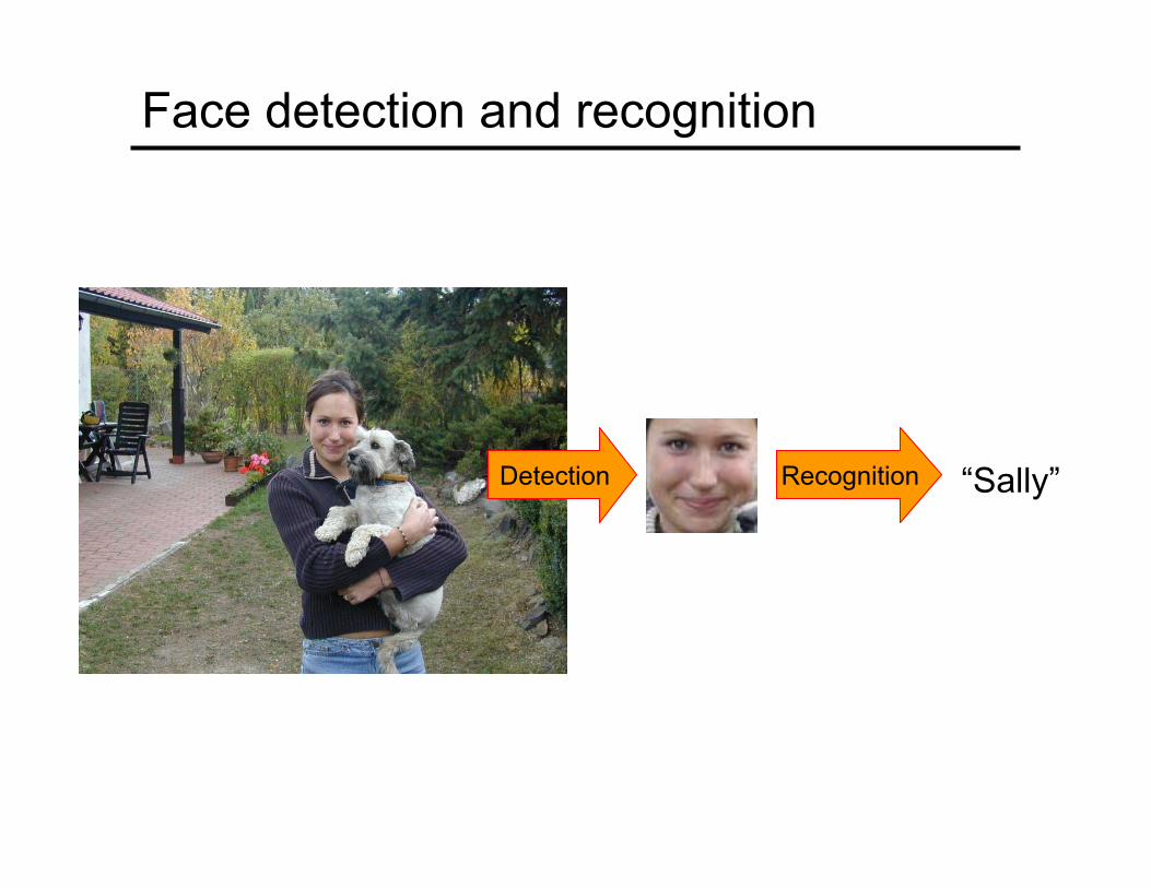
Face detection and recognition
Detection Recognition “Sally”
History
• Early face recognition systems: based on features and distances Bledsoe (1966), Kanade (1973)
• Appearance-based models: eigenfacesSirovich & Kirby (1987), Turk & Pentland (1991)
• Real-time face detection with boosting Viola & Jones (2001)
Outline• Face recognition
• Eigenfaces
• Face detection• The Viola & Jones system
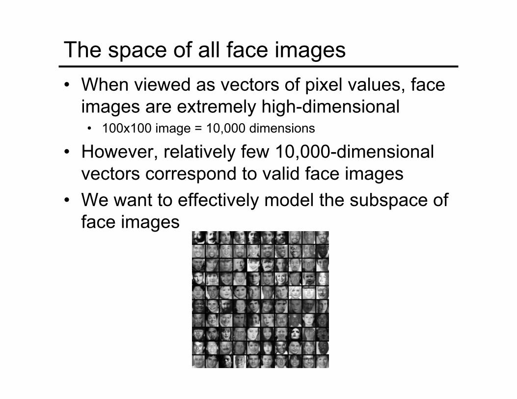
The space of all face images• When viewed as vectors of pixel values, face
images are extremely high-dimensional• 100x100 image = 10,000 dimensions
• However, relatively few 10,000-dimensional vectors correspond to valid face images
• We want to effectively model the subspace of face images

The space of all face images• We want to construct a low-dimensional linear
subspace that best explains the variation in the set of face images

Principal Component Analysis• Given: N data points x1, … ,xN in Rd
• We want to find a new set of features that are linear combinations of original ones:
u(xi) = uT(xi – µ)(µ: mean of data points)
• What unit vector u in Rd captures the most variance of the data?
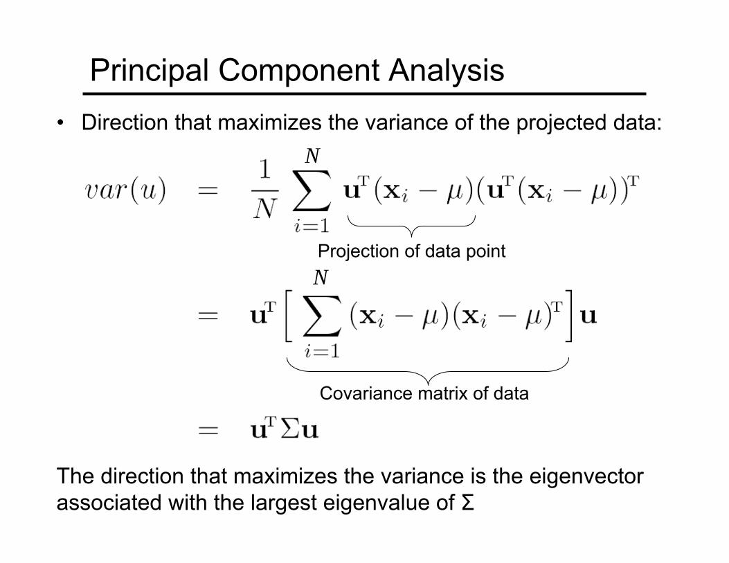
Principal Component Analysis• Direction that maximizes the variance of the projected data:
Projection of data point
Covariance matrix of data
The direction that maximizes the variance is the eigenvector associated with the largest eigenvalue of Σ
N
N

Eigenfaces: Key idea• Assume that most face images lie on
a low-dimensional subspace determined by the first k (k<d) directions of maximum variance
• Use PCA to determine the vectors u1,…ukthat span that subspace:x ≈ μ + w1u1 + w2u2 + … + wkuk
• Represent each face using its “face space”coordinates (w1,…wk)
• Perform nearest-neighbor recognition in “face space”
M. Turk and A. Pentland, Face Recognition using Eigenfaces, CVPR 1991
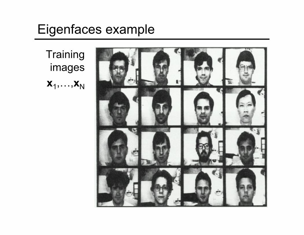
Eigenfaces example
Training images
x1,…,xN

Eigenfaces example
Top eigenvectors:u1,…uk
Mean: μ

Eigenfaces example• Face x in “face space” coordinates:
=

Eigenfaces example• Face x in “face space” coordinates:
• Reconstruction:
= +
µ + w1u1 + w2u2 + w3u3 + w4u4 + …
=
x̂ =
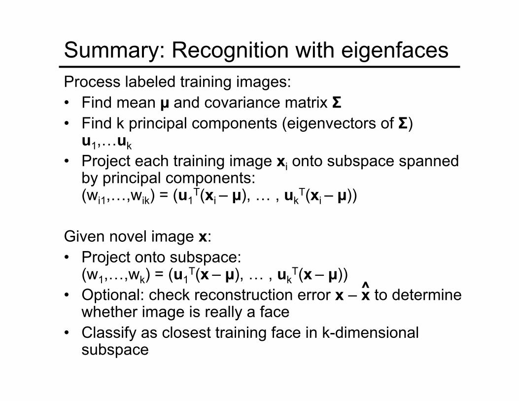
Summary: Recognition with eigenfacesProcess labeled training images:• Find mean µ and covariance matrix Σ• Find k principal components (eigenvectors of Σ)
u1,…uk• Project each training image xi onto subspace spanned
by principal components:(wi1,…,wik) = (u1
T(xi – µ), … , ukT(xi – µ))
Given novel image x:• Project onto subspace:
(w1,…,wk) = (u1T(x – µ), … , uk
T(x – µ))• Optional: check reconstruction error x – x to determine
whether image is really a face• Classify as closest training face in k-dimensional
subspace
^
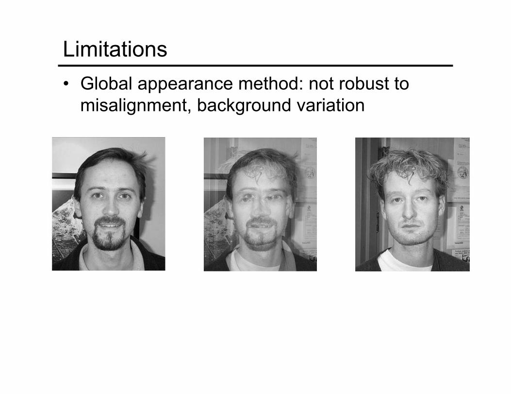
Limitations• Global appearance method: not robust to
misalignment, background variation

Limitations• PCA assumes that the data has a Gaussian
distribution (mean µ, covariance matrix Σ)
The shape of this dataset is not well described by its principal components

Limitations• The direction of maximum variance is not
always good for classification

• Basic idea: slide a window across image and evaluate a face model at every location
Face detection

Challenges of face detection• Sliding window detector must evaluate tens of
thousands of location/scale combinations• This evaluation must be made as efficient as possible
• Faces are rare: 0–10 per image• At least 1000 times as many non-face windows as face windows• This means that the false positive rate must be extremely low• Also, we should try to spend as little time as possible on the non-
face windows

The Viola/Jones Face Detector• A “paradigmatic” method for real-time object
detection • Training is slow, but detection is very fast• Key ideas
• Integral images for fast feature evaluation• Boosting for feature selection• Attentional cascade for fast rejection of non-face windows
P. Viola and M. Jones. Rapid object detection using a boosted cascade of simple features. CVPR 2001.

Image Features
“Rectangle filters”
Value =
∑ (pixels in white area) –∑ (pixels in black area)
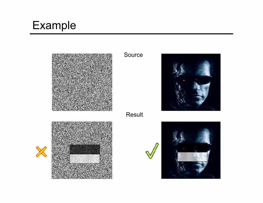
Example
Source
Result
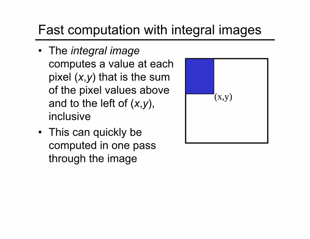
Fast computation with integral images• The integral image
computes a value at each pixel (x,y) that is the sum of the pixel values above and to the left of (x,y), inclusive
• This can quickly be computed in one pass through the image
(x,y)
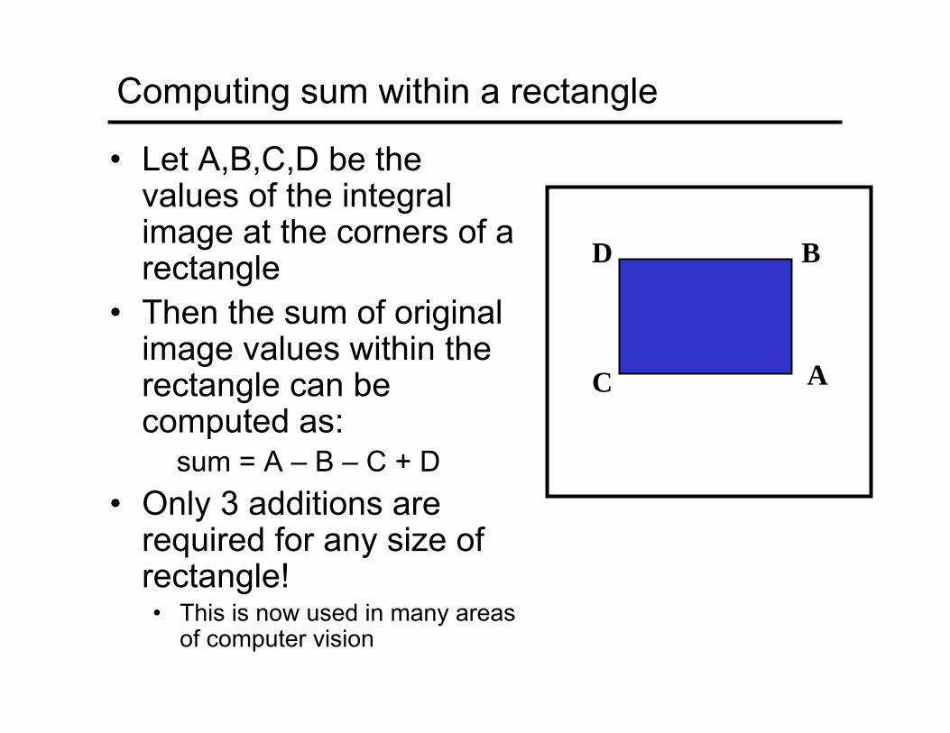
Computing sum within a rectangle
• Let A,B,C,D be the values of the integral image at the corners of a rectangle
• Then the sum of original image values within the rectangle can be computed as:
sum = A – B – C + D• Only 3 additions are
required for any size of rectangle!• This is now used in many areas
of computer vision
D B
C A

Example
-1 +1+2-1
-2+1
Integral Image
(x,y)(x,y)

Feature selection• For a 24x24 detection region, the number of
possible rectangle features is ~180,000!
Feature selection• For a 24x24 detection region, the number of
possible rectangle features is ~180,000! • At test time, it is impractical to evaluate the
entire feature set • Can we create a good classifier using just a
small subset of all possible features?• How to select such a subset?

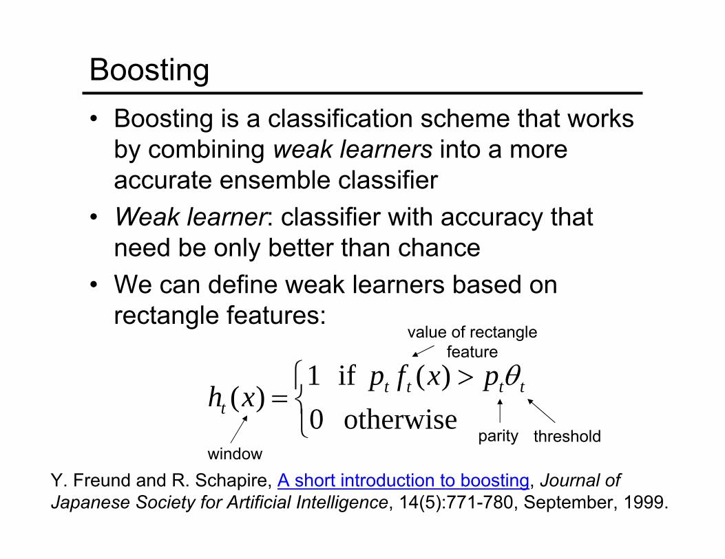
Boosting• Boosting is a classification scheme that works
by combining weak learners into a more accurate ensemble classifier
• Weak learner: classifier with accuracy that need be only better than chance
• We can define weak learners based on rectangle features:
Y. Freund and R. Schapire, A short introduction to boosting, Journal of Japanese Society for Artificial Intelligence, 14(5):771-780, September, 1999.
⎩⎨⎧ >
=otherwise 0
)( if 1)( tttt
t
pxfpxh
θ
window
value of rectangle feature
parity threshold

Boosting outline• Initially, give equal weight to each training
example• Iterative training procedure
• Find best weak learner for current weighted training set• Raise the weights of training examples misclassified by current
weak learner
• Compute final classifier as linear combination of all weak learners (weight of each learner is related to its accuracy)
Y. Freund and R. Schapire, A short introduction to boosting, Journal of Japanese Society for Artificial Intelligence, 14(5):771-780, September, 1999.

Boosting
Weak Classifier 1

Boosting
WeightsIncreased

Boosting
Weak Classifier 2

Boosting
WeightsIncreased
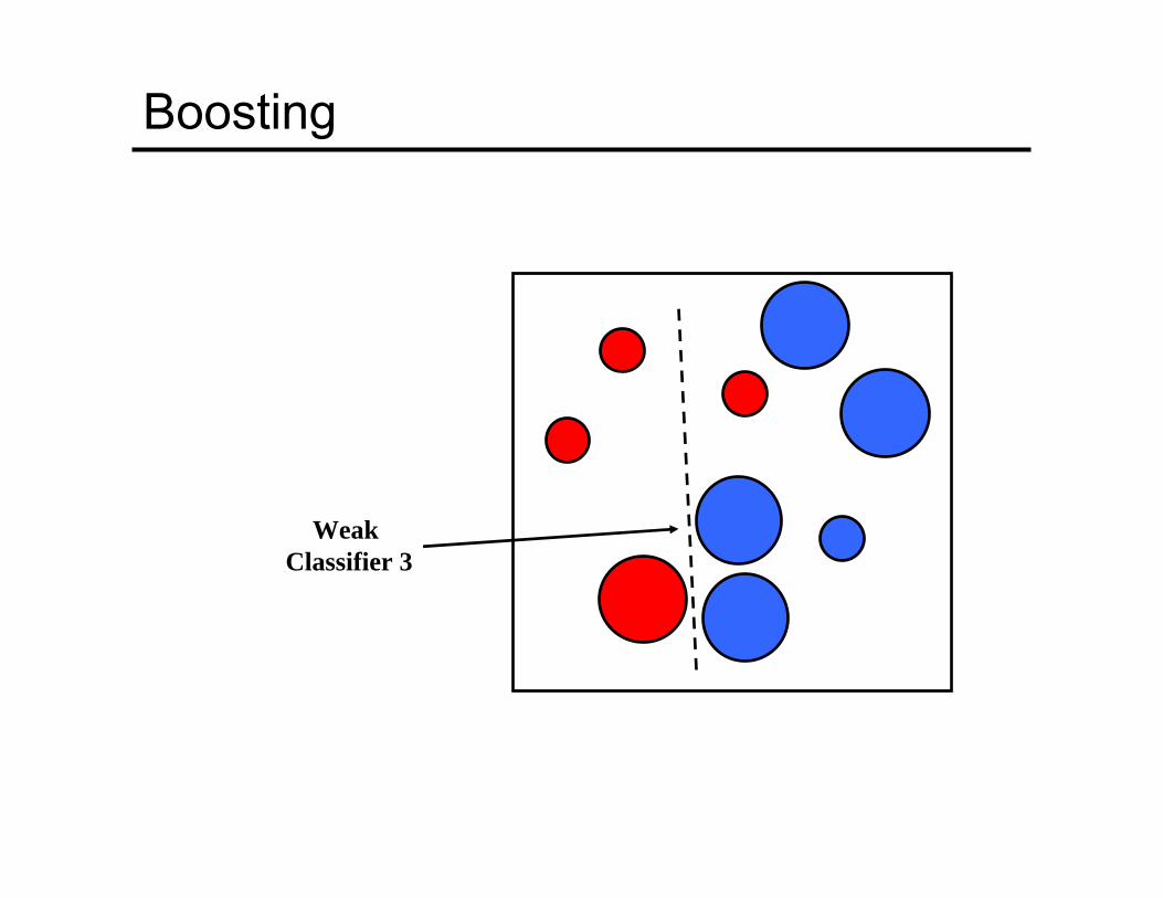
Boosting
Weak Classifier 3
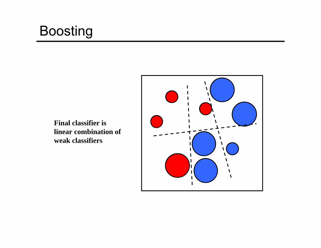
Boosting
Final classifier is linear combination of weak classifiers
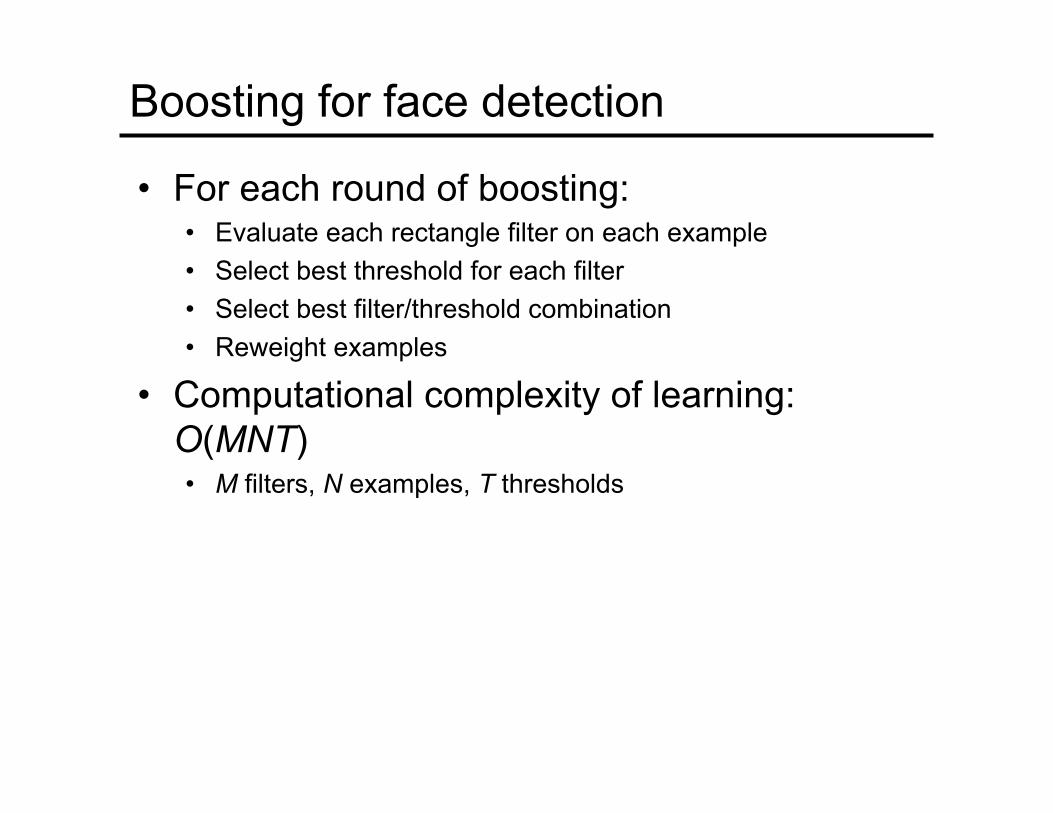
• For each round of boosting:• Evaluate each rectangle filter on each example• Select best threshold for each filter • Select best filter/threshold combination• Reweight examples
• Computational complexity of learning: O(MNT)• M filters, N examples, T thresholds
Boosting for face detection
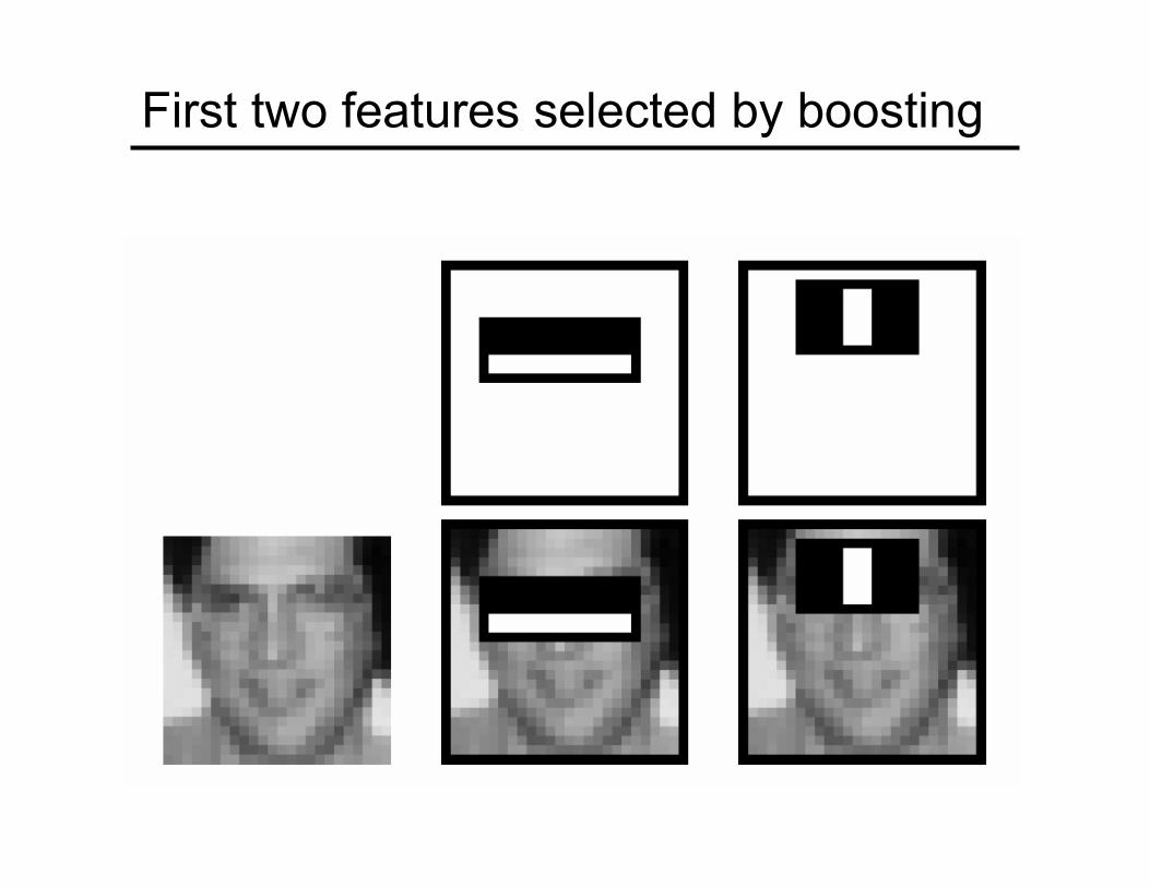
First two features selected by boosting
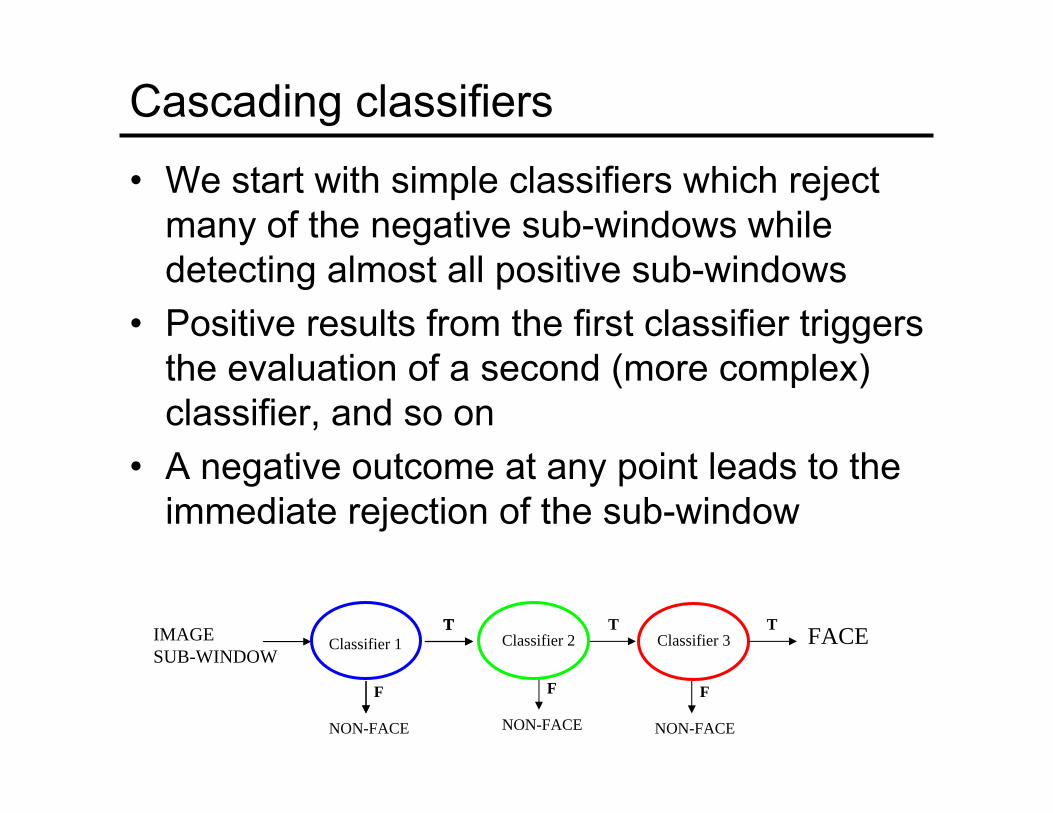
Cascading classifiers
• We start with simple classifiers which reject many of the negative sub-windows while detecting almost all positive sub-windows
• Positive results from the first classifier triggers the evaluation of a second (more complex) classifier, and so on
• A negative outcome at any point leads to the immediate rejection of the sub-window
FACEIMAGESUB-WINDOW
Classifier 1T
Classifier 3T
F
NON-FACE
TClassifier 2
T
F
NON-FACE
F
NON-FACE

Cascading classifiers
• Chain classifiers that are progressively more complex and have lower false positive rates: vs false negdetermined by
% False Pos
% D
etec
tion
0 50
50
100
FACEIMAGESUB-WINDOW
Classifier 1T
Classifier 3T
F
NON-FACE
TClassifier 2
T
F
NON-FACE
F
NON-FACE
Receiver operating characteristic
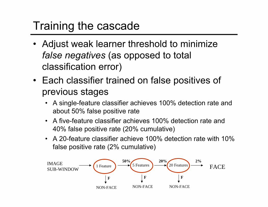
Training the cascade• Adjust weak learner threshold to minimize
false negatives (as opposed to total classification error)
• Each classifier trained on false positives of previous stages• A single-feature classifier achieves 100% detection rate and
about 50% false positive rate• A five-feature classifier achieves 100% detection rate and
40% false positive rate (20% cumulative)• A 20-feature classifier achieve 100% detection rate with 10%
false positive rate (2% cumulative)
1 Feature 5 Features
F
50%20 Features
20% 2%FACE
NON-FACE
F
NON-FACE
F
NON-FACE
IMAGESUB-WINDOW

The implemented system
• Training Data• 5000 faces
– All frontal, rescaled to 24x24 pixels
• 300 million non-faces– 9500 non-face images
• Faces are normalized– Scale, translation
• Many variations• Across individuals• Illumination• Pose
(Most slides from Paul Viola)
System performance• Training time: “weeks” on 466 MHz Sun
workstation• 38 layers, total of 6061 features• Average of 10 features evaluated per window
on test set• “On a 700 Mhz Pentium III processor, the
face detector can process a 384 by 288 pixel image in about .067 seconds”• 15 Hz• 15 times faster than previous detector of comparable
accuracy (Rowley et al., 1998)

Output of Face Detector on Test Images

Other detection tasks
Facial Feature Localization
Male vs. female
Profile Detection

Profile Detection

Profile Features

Summary: Viola/Jones detector• Rectangle features• Integral images for fast computation• Boosting for feature selection• Attentional cascade for fast rejection of
negative windows