F5

Performance Management

The exam

• Five compulsory questions: 20 marks

each

• Time allowed: 3hours plus 15 minutes

reading time

• Balance typically 50:50 between

calculations and discussion aspects

The examiner’s key concerns

• Students need to be able to interpret any numbers they calculate and see the limitations of their financial analysis.

• In particular financial performance indicators may give a limited perspective and NFPIs are often needed to see the full picture.

• Questions will be practical and realistic, so will not dwell on unnecessary academic complications.

• Many questions will be designed so discussion aspects can be attempted even if students have struggled with calculation aspects.

1. Advanced costing methods

• ABC.

• Target costing.

• Lifecycle costing.

• Throughput accounting.

• Environmental Accounting

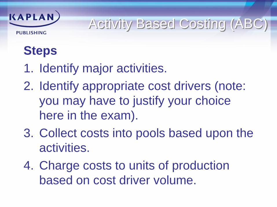
Activity Based Costing (ABC)

Steps

1. Identify major activities.

2. Identify appropriate cost drivers (note:

you may have to justify your choice

here in the exam).

3. Collect costs into pools based upon the

activities.

4. Charge costs to units of production

based on cost driver volume.

Activity Based Costing (ABC)

Cost driver rate = total driver pool cost

cost driver volume

Advantages of ABC

• More realistic costs.

• Better insight into cost drivers, resulting in better cost control.

• Particularly useful where overhead costs are a significant proportion of total costs.

• ABC recognises that overhead costs are not all related to production and sales volume.

• ABC can be applied to all overhead costs, not just production overheads.

• ABC can be used just as easily in service costing as in product costing.

Criticisms of ABC

• It is impossible to allocate all overhead

costs to specific activities.

• The choice of both activities and cost

drivers might be inappropriate.

• ABC can be more complex to explain to

the stakeholders of the costing exercise.

• The benefits obtained from ABC might

not justify the costs.

Implications of ABC

• Pricing - more realistic costs improve

cost-plus pricing.

• Sales strategy - more realistic margins

can help focus sales strategy.

• Decision making – for example,

research and development can be

directed at products with better margins.

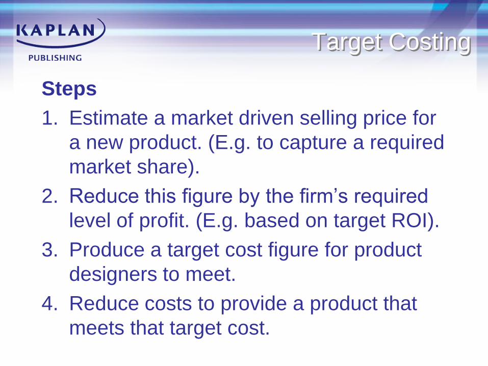
Target Costing

Steps

1. Estimate a market driven selling price for

a new product. (E.g. to capture a required

market share).

2. Reduce this figure by the firm‟s required

level of profit. (E.g. based on target ROI).

3. Produce a target cost figure for product

designers to meet.

4. Reduce costs to provide a product that

meets that target cost.

Closing the target cost gap

• Value analysis

• Focus is on reducing cost without

compromising perceived value.

• Can labour savings be made?

• Can productivity be improved?

• What production volume is needed to

achieve economies of scale?

Closing the target cost gap –

cont.

• Could cost savings be made by

reviewing the supply chain?

• Can any materials be eliminated?

• Can a cheaper material be substituted

without affecting quality?

• Can part-assembled components be

bought in to save on assembly time?

• Can the incidence of the cost drivers be

reduced?

Implications of target

costing• Pricing – might identify sufficient cost

savings to reduce the target price.

• Cost control – target cost motivates

managers to find new ways of saving

costs.

Lifecycle costing

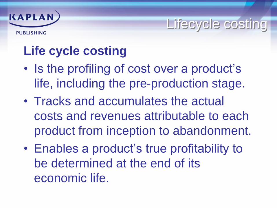
Life cycle costing

• Is the profiling of cost over a product‟s

life, including the pre-production stage.

• Tracks and accumulates the actual

costs and revenues attributable to each

product from inception to abandonment.

• Enables a product‟s true profitability to

be determined at the end of its

economic life.

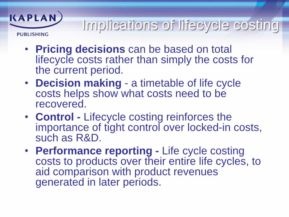
Implications of lifecycle costing

• Pricing decisions can be based on total lifecycle costs rather than simply the costs for the current period.

• Decision making - a timetable of life cycle costs helps show what costs need to be recovered.

• Control - Lifecycle costing reinforces the importance of tight control over locked-in costs, such as R&D.

• Performance reporting - Life cycle costing costs to products over their entire life cycles, to aid comparison with product revenues generated in later periods.

Throughput

Background

• Application of key factor analysis to

production bottlenecks.

• The only totally variable costs are the

purchase cost of raw materials /

components

• Direct labour costs are not wholly

variable.

Throughput

Multi-product decisions

• Rank products by looking at the

throughput per hour of bottleneck

resource time

• Throughput = Revenue – Raw Material

Costs

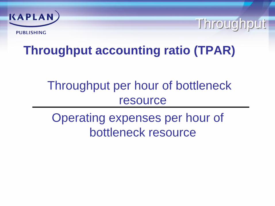
Throughput

Throughput accounting ratio (TPAR)

Throughput per hour of bottleneck

resource

Operating expenses per hour of

bottleneck resource

Throughput

How to improve the TPAR

• Increase the sales price to increase the

throughput per unit.

• Reduce total operating expenses, to

reduce the cost per hour.

• Improve productivity, reducing the time

required to make each unit of product.

Contribution = Sales Value – All Variable Costs

Units 0 100 500 1000 1500

Contribution(£) 0 1000 5000 10000 15000

Fixed Costs(£) (10000) (10000) (10000) (10000) (10000)

Profit(£) (10000) (9000) (5000) 0 5000

Profit = (Contribution per unit x units) - Fixed Costs

A product has a sales price of £20 and a variable cost of £10 per unit

Contribution per unit 10 10 10 10

Profit per unit 0 (90) (10) 50

2. CVP Analysis

Environmental costs

Environmental costs

Internal costs directly impact on the income statement of a company.

improved systems

waste disposal

costs

product take back

costs

regulatory costs

upfront costs

backend

Costs

External Costs are imposed on society at large but not borne by the company that generates the cost in the first instance

carbon emissions

usage of energy and

water

forest degradation

health care costs

social welfare costs

Break-even analysis

The Break-even chart

£

Output (units)

Fixed Costs

Breake

ven

Point

Breakeven point:

The point where

total costs = total

sales revenueand

Where there is

neither a profit or

loss

B/E Point (units) = Fixed Costs

Contribution per Unit

Chapter 4

The Margin of Safety

£

Fixed Costs

Sales Revenue

Total Costs

Breakeven

Output

Budgeted

Output

Margin of safety

The Margin of Safety represents the level by which output can fall

before the organisation makes a loss

Margin of Safety = Budgeted Output – Breakeven Output

Budgeted Output

X 100%

Chapter 4

Contribution to Sales ratio

Chapter 4

Contribution to Sales Ratio (C/S ratio)

=

(Contribution per unit) / Unit Sales Price

Breakeven Point in Sales Value

=

Fixed Costs / C/S ratio

Sales for a certain level of profit = Fixed Costs + Required Profit

Contribution per Unit

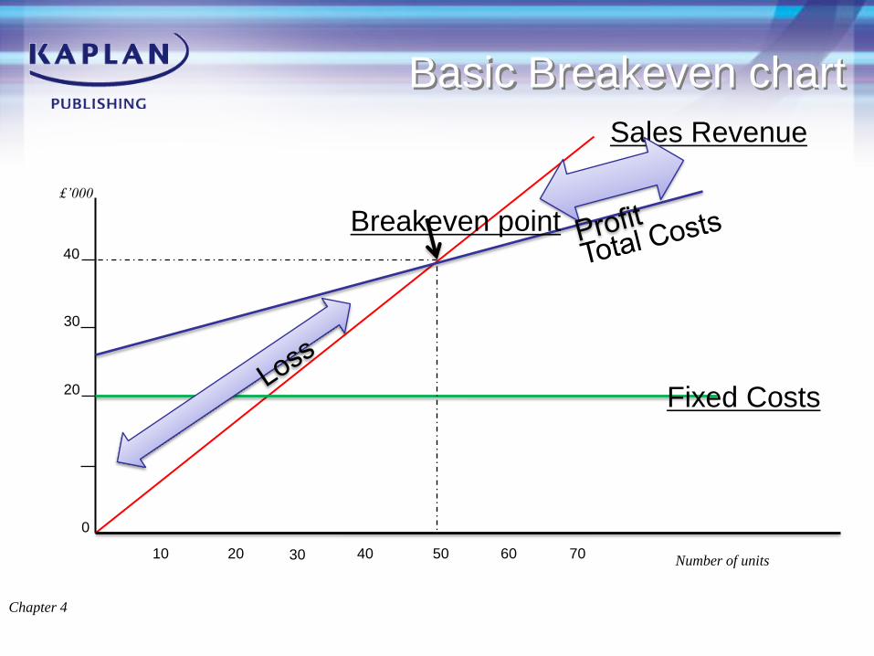
Basic Breakeven chart

Chapter 4

0

Sales Revenue

10

20

30

Fixed Costs

40

Breakeven point

20 30 40 50 60 70Number of units

£’000

Contribution Breakeven chart

Sales Revenue

10

Variable Costs

Breakeven point

20 30 40 50 60 70Number of units

£’000

Fixed Costs

Contribution

Chapter 4

The Profit-Volume Chart

The profit-volume chart presents information in a way that clearly shows

the change in the level of profit – using data from the previous data table:

0

+£5000

-£10000

1000 1500

Profit

Output

Page 30

Chapter 4

Limitations/Assumptions of

CVP

Costs behaviour is assumed to be linear

Revenue is assumed to be linear

Volume Produced = Volume Sold

Ignores inflation

Assumes a constant sales mix

Chapter 4

3. Planning with limited factors

• Key factor analysis – one resource

in short supply

• Linear Programming – two or more

scarce resources

Key factor analysis

1. Calculate contribution per unit.

2. Calculate contribution per unit of the

limiting factor.

3. Rank in order.

4. Allocate resources – make first up to

max demand, then second,...

Linear programming

1. Define variables

2. Define the objective

3. Set out constraints

4. Draw graph showing constraints and

identify the feasible region

5. Identify optimal point

6. Solve for optimal solution

7. Answer the question

Linear programming

Assumptions

• A single quantifiable objective.

• Each product always uses the same

quantity of the scarce resources per

unit.

• The contribution per unit is constant.

• Products are independent – e.g. sell A

not B.

• The scenario is short term.

Linear programming

Slack

• Slack is the amount by which a

resource is under utilized. It will occur

when the optimum point does not fall on

the given resource line.

Linear programming

Shadow (or dual) prices

• The extra contribution that results from

having one extra unit of a scarce

resource.

• The max premium (i.e. over the normal

cost) that the firm should be willing to

pay for one extra unit of each constraint.

• Non-critical constraints will have zero

shadow prices as slack exists already.

Linear programming

Calculating dual prices

1. Add one unit to the constraint

concerned, while leaving the other

critical constraint unchanged.

2. Solve the revised equations to derive a

new optimal solution.

3. Calculate the revised optimal

contribution. The increase is the

shadow price

Linear programming

Range of applicability of dual prices

• The dual price only applies as long as

extra resources improve the optimal

solution

• i.e. the constraint line concerned moves

out increasing the size of the feasible

region and moving the optimal point.

• Eventually other constraints become

critical.

4. Pricing

• Factors to consider when pricing.

• Calculation aspects.

• Pricing approaches.

Factors to consider when pricing

• Costs

• Competitors

• Corporate objectives

• Customers

Calculation aspects

Price elasticity of demand (PED)

• PED = % change in demand / %

change in price.

• PED >1 (elastic) revenue increases if

the price is cut.

• PED <1 (inelastic) revenue increases if

the price is raised.

Calculation aspects

Equation of a straight line demand

curve

• P = a – bQ

• “a” = the price at which demand would

fall to zero

• “b” = gradient = change in price/change

in demand

• Calculate “b” first

Calculation aspects

Equation of a cost curve

• C = F + vQ

• Volume based discounts

Pricing approaches

• Cost plus pricing

• Price skimming

• Penetration pricing

• Linking pricing decisions for different

products

• Volume discounts

• Price discrimination

• Relevant cost pricing

Cost plus pricing

• Establish cost per unit – options include

MC, TAC, prime cost

• Calculate price using target mark-up or

margin

• Often used as a starting point even

when using other methods

Cost plus pricing

Advantages

• Widely used and accepted.

• Simple to calculate if costs are known.

• Selling price decision may be delegated

to junior management.

• Justification for price increases.

• May encourage price stability.

Cost plus pricing

Disadvantages

• Ignores link between price and demand.

• No attempt to establish optimum price.

• Which absorption method?

• Does not guarantee profit

• Which cost?

• Inflexibility in pricing.

• Circular reasoning.

Price skimming

• Set a high initial price to „skim off‟

customers who are willing to pay extra.

• Prices fall over time.

• Suitability?

Penetration pricing

• Set a low initial price to gain market

share

• If a high volume is achieved, the low

price could be sustainable.

• Suitability?

Linking pricing decisions for

different products

• Basic idea: product A is cheap to attract

customers who then also buy the higher

margin product B.

• Key issue is the extent to which

customer must buy the other products.

• Suitability?

Volume discounts

• Discount for individual large order.

• Cumulative quantity discounts.

• Suitability?

Price discrimination

• Have different prices in different

markets for the same product.

• Suitability?

Relevant cost pricing

• Price = net incremental cash flow.

• Suitability?

5. Make v buy and other short

term decisions

• Relevant costing principles.

• Make v buy decisions.

• Shut down decisions.

• Joint products – the further processing

decision.

Relevant costing principles

• Include

– Future incremental cash flows.

– Opportunity costs

• Exclude

– Depreciation.

– Sunk costs.

– Unavoidable costs.

– Apportioned fixed overheads.

– Financing cash flows (e.g. interest).

Make v buy

Decision

• Look at future incremental cash flows.

• Watch out for opportunity costs –

especially whether or not spare capacity

exists and alternative uses for capacity.

• Practical factors?

Shut down decisions

Decision

• Look at future incremental cash flows.

– Apportioned overheads not relevant

– Closure costs – e.g. redundancies.

– Alternative uses for resources?

• Practical factors?

Joint products

The further processing decision

• Look at future incremental cash flows:

– sell at split off v process further and then

sell.

• Pre-separation (“joint”) costs not

relevant

– only include post split-off aspects.

6. Risk and uncertainty

• Basic concepts.

• Research techniques.

• Scenario planning.

• Simulation.

• Expected values.

• Sensitivity.

• Payoff tables.

Basic concepts

• Risk = variability in future returns.

• Investors‟ risk aversion

• Upside v downside

• Risk v uncertainty

• Risk = probability x impact

Research techniques

• Desk research

– Company records.

– General economic intelligence.

– Specific market data.

• Field research

– Opinion v motivation v measurement

– Questionnaires, experiments, observation.

– Group interviews, triad testing, focus

groups.

Scenario planning

1 Identify high-impact, high-uncertainty

factors.

2 Identify different possible futures.

3 Identify consistent future scenarios.

4 “Write the scenario”.

5 For each scenario identify and assess

possible courses of action for the firm.

6 Monitor reality.

7 Revise scenarios and strategic options

Simulation

1 Apply probabilities to key factors in

scenario analysis.

2 Use random numbers to select a

particular scenario and calculate

outcome.

3 Repeat until build up a picture of

possible outcomes

4 Make decision based on risk aversion.

Expected values

• EV = Σ outcome × probability.

• Make decision based on best EV.

Expected values

Advantages

• Recognises that there are several

possible outcomes.

• Enables the probability of the different

outcomes to be taken into account.

• Leads directly to a simple optimising

decision rule.

• Calculations are relatively simple.

Expected values

Disadvantages

• probabilities used are subjective.

• EV is the average payoff. Not useful for

one-off decisions.

• EV gives no indication of risk

• Ignores the investor‟s attitude to risk.

Sensitivity

• Identify key variables by calculating how

much an estimate can change before

the decision reverses.

• Can only vary one estimate at a time.

Payoff tables

• Prepare table of profits based on

different decision choices and different

possible scenarios.

• Four different ways of making a

decision.

– 1 Expected values

– 2 Maximax

– 3 Maximin

– 4 Minimax regret

7. Budgeting I

• The purposes of budgeting.

• Budgets and performance

management.

• The behavioural aspects of budgeting.

• Conflicting objectives.

The purpose of budgets

• Forecasting

• Planning

• Control

• Communication

• Co-ordination

• Evaluation

• Motivation

• Authorisation and delegation

Budgets and performance

management

Responsibility accounting

• Responsibility accounting divides the

organisation into budget centres, each

of which has a manager who is

responsible for its performance.

• The budget is the target against which

the performance of the budget centre or

the manager is measured.

Management by exception

1 Set up standard costs, prepare budgets

and set targets.

2 Measure actual.

3 Compare actual to budget (e.g. via

variances).

4 Investigate reasons for differences and

take action.

Behavioural aspects of budgeting

Key issues

– Dysfunctional behaviour – want goal

congruence.

– Budgetary slack.

Management styles (Hopwood)

– Budget constrained

– Profit conscious

– Non-accounting

Target setting and motivation

• Expectations v aspirations

• Ideal target?

• Targets should be:

– communicated in advance

– dependent on controllable factors

– based on quantifiable factors

– linked to appropriate rewards

– chosen to ensure goal congruence.

Participation

Advantages of participative budgets

• Increased motivation

• Should contain better information,

• Increases managers‟ understanding and

commitment

• Better communication

• Senior managers can concentrate on

strategy.

Participation

Disadvantages of participative budgets

• Loss of control

• Inexperienced managers

• Budgets not in line with objectives

• Budget preparation slower and disputes

can arise

• Budgetary slack

• Certain environments may preclude

participation

Conflicting objectives

• Company v division

• Division v division

• Short-termism

• Individualism

8. Budgeting II

• Rolling v periodic.

• Incremental budgeting.

• Zero based budgeting (ZBB).

• Activity based budgeting (ABB).

• Feedforward control.

• Flexible budgeting.

• Selecting a budgetary system.

• Dealing with uncertainty.

• Use of spreadsheets.

Rolling v periodic budgeting

Periodic budgets

• The budget is prepared for typically one

year at a time. No alterations once the

budget has been set.

• Suitable for stable businesses where

forecasting is easy and where tight

control is not necessary.

Rolling v periodic budgeting

Rolling (continuous) budgets

• A budget kept continuously up to date

by adding another accounting period

when the earliest period has expired.

• Aim: to keep tight control and always

have an accurate budget for the next 12

months.

• Suitable if accurate forecasts cannot be

made, or if need tight control.

Incremental budgeting

• Start with the previous period‟s budget

or actual results and add (or subtract)

an incremental amount to cover inflation

and other known changes.

• Suitable for stable businesses where

costs are not expected to change

significantly. There should be good cost

control and limited discretionary costs.

Zero based budgeting

Preparing a budget from a zero base,

justifying all expenditure.

1 Identify all possible services and then cost

each service (decision packages)

2 Rank the decision packages

3 Identify the level of funding that will be

allocated to the department.

4 Use up the funds in order of the ranking

until exhausted.

Activity based budgeting

• Use ABC for budgeting purposes:

1 Identify cost pools and cost drivers.

2 Calculate a budgeted cost driver rate

3 Produce a budget for each department or

product by multiplying the budgeted cost

driver rate by the expected usage.

Feed forward control

• Feed-forward control is defined as the

„forecasting of differences between

actual and planned outcomes and the

implementation of actions before the

event, to avoid such differences.

• E.g. using a cash-flow budget to

forecast a funding problem and as a

result arranging a higher overdraft well

in advance of the problem.

Flexible budgeting

• Fixed Budgets

• Flexible Budgets

• Flexed Budgets

Selecting a budgetary system

Determinants

• Type of organisation.

• Type of industry.

• Type of product and product range.

• Culture of the organisation.

Changing a budgetary system

Factors to consider

• Time consuming

• Are suitably trained staff are available to

implement the change successfully?

• Management time

• Training needs.

• Cost v benefits for the new system:

Incorporating risk and uncertainty

• Flexible budgeting.

• Rolling budgets.

• Scenario planning.

• Sensitivity analysis.

• “What if” analysis using spreadsheets

9. Quantitative analysis

• High-low.

• Regression and correlation.

• Time series analysis.

• Learning curves.

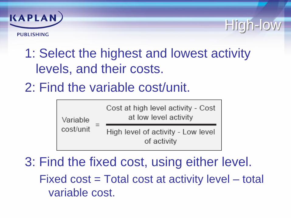
High-low

1: Select the highest and lowest activity

levels, and their costs.

2: Find the variable cost/unit.

3: Find the fixed cost, using either level.

Fixed cost = Total cost at activity level – total

variable cost.

Regression and correlation

y = a + bx

22 x)(-xn

yx-xyn

n

xb

n

y

)y)(-y(n )x)(-xn

yx-xyn

2222

r =

Time series analysis

• Four components:

1 the trend

2 cyclical variations

3 seasonal variations

4 residual variations.

• Additive model

Actual = Trend + Seasonal Variation

• Multiplicative model

Actual = Trend x Seasonal Variation

Learning curves

• As cumulative output doubles, the

cumulative average time per unit falls to

a fixed % (the learning rate) of the

previous average.

• Y = axb

y = average cost per batch

a = cost of first batch

x = total number of batches produced

b = learning factor (log LR/log 2)

10. Standard costing and basic

variances

• Standard costing.

• Recap of basic variances from F2.

• Labour variances with idle time.

• Variance investigation.

Standard costing

• A pre-determination of what a product is

expected to cost under specific working

conditions.

Standard costing

Advantages

– Annual detailed examination

– Performance appraisal

– Management by exception

– Simplifies bookkeeping

• Disadvantages / problems

– Standards not updated

– Cost

– Unrealistic standards can demotivate staff

Types of standard

• Attainable

• Ideal

• Basic

• Current

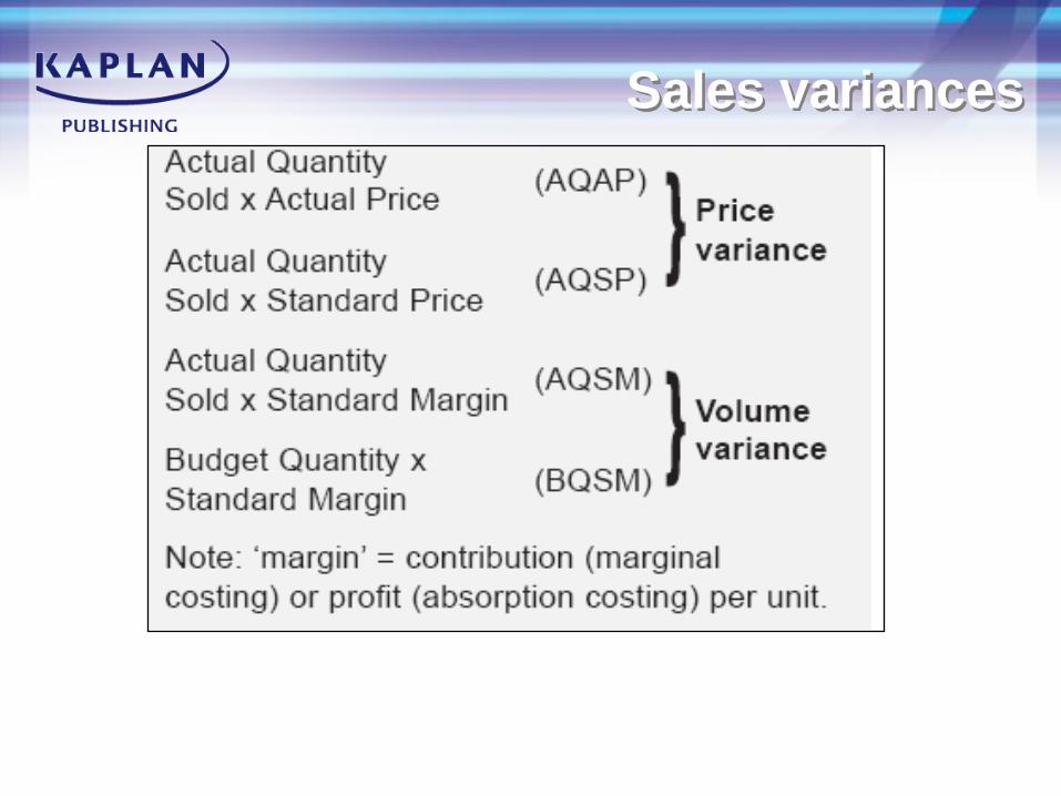
Sales variances

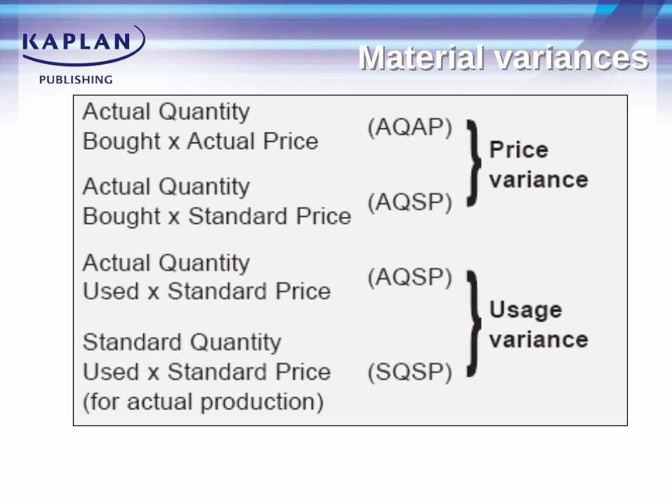
Material variances

Labour variances (basic)

Variable overhead variances

Fixed overhead variances

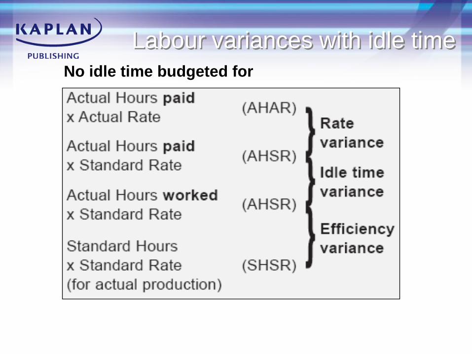
Labour variances with idle time

No idle time budgeted for

Idle time budgeted for

Variance investigation

11. Advanced variances

• Materials mix and yield variances.

• Other targets for controlling production.

• Planning and operational variances.

• Modern manufacturing environments.

Materials mix and yield variances

• Only use where materials can be

substituted for each other.

Other targets for controlling

production processes

• Detailed timesheets, % idle time.

• Productivity, % yield, % waste.

• Quality measures e.g. reject rate.

• Average cost of inputs, output.

• Average margins.

• % on-time deliveries.

• Customer satisfaction ratings.

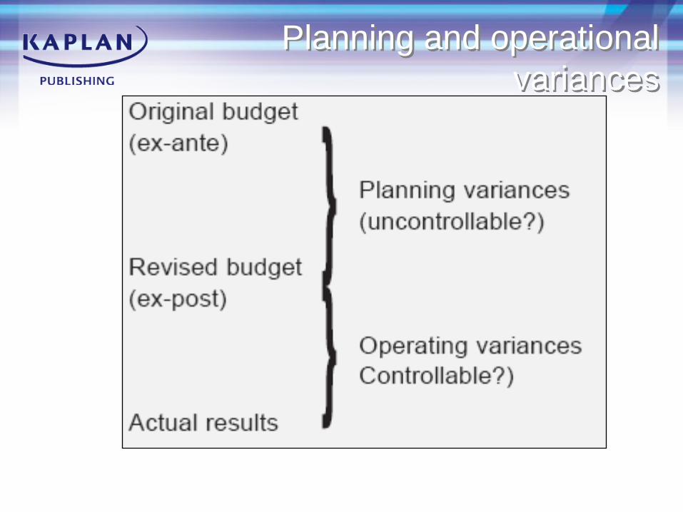
Planning and operational

variances

Market size and market

shares variances

Planning and operating cost

variances

Modern manufacturing

environments

Total Quality Management (TQM)

• TQM is the continuous improvement in

quality, productivity and effectiveness

through a management approach

focusing on both process and the

product.

Modern manufacturing

environments

Just-in–time (JiT)

• JIT is a pull-based system of planning

and control.

• Pulling work through the system in

response to customer demand.

• Goods are only produced when they are

needed.

• This eliminates large inventories of

materials and finished goods.

12. Performance

measurement and control

• Ratio analysis.

• NFPIs.

• Behavioural considerations.

Ratio analysis

Preliminaries

• Ratios may not be representative of the

position throughout a period.

• Need a basis for comparison.

• Ratios can be manipulated

• Ratios indicate areas for further

investigation rather than giving answers.

Profitability ratios

• ROCE = Operating Profit x 100%

Capital Employed

• Gross margin = Gross profit x 100%

Sales

• Net margin = Net profit x 100%

Sales

• Asset turnover = Sales / capital employed

• ROCE = asset turnover x net margin

Liquidity / working capital ratios

• Current ratio = current assets / current liabilities

• Quick ratio = quick assets/ current liabilities

Quick assets = current assets – inventory

• Receivables days = receivables / sales x 365

• Payables days = payables / purchases x 365

• Inventory days = inventory / cost of sales x 365

Ratios to measure risk

• Financial gearing = debt/equity

• Financial gearing = debt / (debt + equity)

• Dividend cover = PAT / total dividend

• Interest cover = PBIT / interest

• Operating gearing = fixed costs / variable costs

• Operating gearing = contribution / PBIT

Non-financial performance

indicators

• Financial performance appraisal often

reveals the ultimate effects of

operational factors and decisions but

non-financial indicators are needed to

monitor causes.

• Critical success factors often non-

financial

• Stakeholder objectives may also be

non-financial

The balanced scorecard

(Kaplan and Norton)

The building block model

(Fitzgerald et al)

Behavioural aspects

• Measures designed to assess

performance should:

– provide incentives to promote goal

congruence.

– only incorporate factors for which the

manager can be held responsible.

– recognise both financial and non financial

aspects of performance.

– recognise longer-term, as well as short

term, objectives.

Behavioural aspects

• Potential problems with inappropriate

measures

– manipulation of information provided by

managers

– demotivation and stress-related conflict

– excessive concern for control of short term

costs, possibly at the expense of longer-

term profitability.

• Transfer pricing.

• Divisional performance measurement.

13. Transfer pricing and

divisional

Performance measurement

Transfer pricing

Objectives

• Goal congruence

• Performance measurement.

• Autonomy.

• Minimising global tax liability.

• To record the movement of goods and

services.

• Fair split of profit between divisions.

Transfer pricing

- Exam questions

Will often be given a TP and asked to

comment. Look at the following.

• Implications for divisional performance –

e.g. is a target ROI achieved?

• Resulting manager behaviour - does it

give dysfunctional decision making –

e.g. will a manager reject a new product

that is acceptable to the company as a

whole?

Transfer pricing

- General rule

• TP = marginal cost + opportunity cost

• In a perfectly competitive market,

TP = market price.

• If spare capacity exists,

TP = marginal cost.

• With production constraints,

TP = marginal cost + opportunity cost of not

using those resources elsewhere.

Practical transfer pricing

systems

• Market price

• Production cost + mark-up

• Negotiation

Divisional performance

measurement

Key considerations

• Manager or division?

• Type of division.

– Cost centre

– Profit centre

– Investment centre

Return on Investment (ROI)

Residual Income (RI)

RI = Pre tax controllable profits – imputed

charge for controllable invested capital

14. Performance measurement

in not-for-profit organisations

• Objectives.

• Performance Measurement.

Objectives

Planning for NFPs usually more complex.

• Multiple objectives

• Difficult to quantify objectives

• Conflicts between stakeholders

• Difficult to measure performance

• Different ways to achieve the same

objective

• Objectives may be politically driven

Performance measurement

Value for money (VFM)

• Effectiveness

• Efficiency

• Economy