f undamen tals of plasma ph ysicsgedalin/teaching/mater/plasma3.pdf · "c j.d callen, f...
TRANSCRIPT
Fundamentals of
Plasma Physics
James D. CallenUniversity of Wisconsin, Madison
June 3, 2003
PREFACE
Plasma physics is a relatively new branch of physics that became a maturescience over the last half of the 20th century. It builds on the fundamental areasof classical physics: mechanics, electrodynamics, statistical mechanics, kinetictheory of gases, and fluid mechanics. The distinguishing feature of the plasmamedium is that its properties are determined by the nature of the interactionsbetween the charged particles in it — collective rather than binary and weakcompared to their thermal motions.
The collective but weak interactions in a plasma embody many physicalprocesses over a wide range of length and time scales: predominantly deter-ministic particle motion which however may be diffusive on long time scales,internal generation of microscopically irregular but macroscopically smooth elec-tromagnetic fields, both adiabatic and inertial (or fluidlike) plasma responses,dielectric medium type electrical properties, and various flow regimes (laminar,transitional, shock and turbulent). These processes lead to a wide variety ofinteresting collective phenomena, e.g., dielectric shielding of charges, waves inthe medium, transfer of energy from waves to particles (via Landau damping, a“collisionless” wave-particle resonance effect), transfer of energy from a distribu-tion of particles into waves (instabilities), and turbulence in the six-dimensional(three real plus three velocity space coordinates) phase space.
Increased understanding of plasma physics has both been stimulated by, andpaced, the development of its many important applications, e.g., magnetic andinertial approaches to fusion, space and astrophysical plasmas, plasma process-ing of materials, and coherent radiation generation (typically via acceleration ofbeams of electrons or ions). Thus, plasma physics has developed in large partas a branch of applied or engineering physics — “science with a purpose.”
The primary objective of this book is to present and develop the fundamen-tals and principal applications of plasma physics, with an emphasis on whatis usually called high-temperature plasma physics where the plasma is nearlyfully ionized with nearly negligible effects of neutral particles on the plasmabehavior. The level is meant to be suitable for senior undergraduate studentsthrough advanced graduate students and active researchers. Pedagogically, itbegins from an elemental or microscopic description, then uses this to developmacroscopic models of plasmas, and finally uses these models to discuss prac-tical applications. A variety of applications of plasma physics are discussedthroughout the text; many others are covered in the problems at the end ofeach chapter. In concert with the modern trend in the physical sciences, SI(Systeme International d’Unites) or mks units are used throughout.
This book has evolved primarily from lecture notes developed while teach-ing various plasma physics courses at the University of Wisconsin-Madison overmore than two decades (1979–2003) and in part from teaching three years atMassachusetts Institute of Technology (1969–1972). My own research and teach-ing has been predominantly in magnetic fusion research, which has been thedominant driving force behind the development of the science of plasma physicsover this period. However, because plasma physics has grown into a mature
i
PREFACE ii
science whose principles are broadly applicable, I attempt to develop the fun-damental concepts in an application-independent manner. In addition, manydifferent types of applications of plasma physics are discussed throughout thebook.
The science of plasma physics draws heavily on many areas of classicalphysics and applied mathematics. Typically, not all of these subjects are wellknown to the wide variety of students (from physics, engineering physics, elec-trical engineering, nuclear engineering and other undergraduate curricula) whobegin studies of plasma physics. Also, most of the needed background materialis not readily available in concise, accessible forms. Thus, a number of Ap-pendices have been written to provide relevant summaries; they give importantsupplementary information that is an integral part of this textbook. Finally,“Appendix Z” (to be placed on pages inside book covers) provides sets of ba-sic formulas that are useful throughout the book — vector relations, vectordifferentiation operators, physical constants, and key plasma formulas.
This book is designed for teaching plasma physics at a variety of levels.(It may also serve as a useful reference book for active researchers in plasmaphysics.) For example, it could be used as the basis for a two (or more) semestergraduate-level course on plasma physics, at the rate of approximately one chap-ter section per one hour lecture. However, it could also be used for teachinga fast-paced, one-semester introductory course on plasma physics by coveringonly the sections at the first of most of the chapters. Intermediate-level subjectsthat could be omitted without compromising understanding of later sections areindicated by an asterisk (*) at the end of the respective section titles. Advancedmaterial, which is relevant mostly for research purposes, is similarly indicatedby a plus sign (+). Bibliographies at the end of each of the chapters and appen-dices provide information on other textbooks and research literature that shouldbe consulted for further details or supplementary course material. Individualchapters of this book will be made available (in draft form) via my public webpage (http://www.cae.wisc.edu/∼callen) as soon as they are available.
The large number of problems at the end of each chapter are graduated inlevel of difficulty commensurate with the various levels and styles of courses thatmight be taught from the book. Specifically, the levels of the problems are clas-sified according to their nature and consequent degree of difficulty: evaluational(/), application development (//) and conceptual development (///). Also, thelevel of material involved in solving the problem is indicated: basic (no mark),intermediate (*), or advanced (+).
(Detailed acknowledgements of help by others and assistance in the prepa-ration of this manuscript will be written later.)
DRAFT 10:38June 3, 2003
PREFACEc©J.D Callen, Fundamentals of Plasma Physics
iii
Introduction
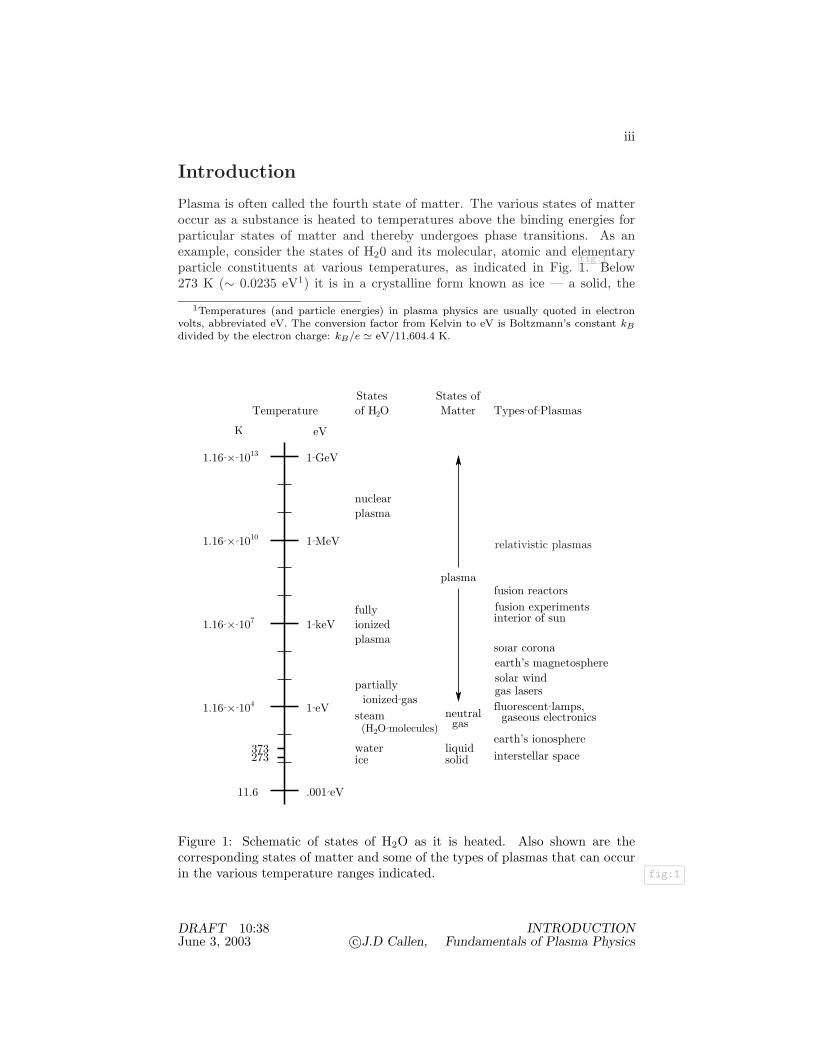
Plasma is often called the fourth state of matter. The various states of matteroccur as a substance is heated to temperatures above the binding energies forparticular states of matter and thereby undergoes phase transitions. As anexample, consider the states of H20 and its molecular, atomic and elementaryparticle constituents at various temperatures, as indicated in Fig.
fig:11. Below
273 K (∼ 0.0235 eV1) it is in a crystalline form known as ice — a solid, the
1Temperatures (and particle energies) in plasma physics are usually quoted in electronvolts, abbreviated eV. The conversion factor from Kelvin to eV is Boltzmann’s constant kB
divided by the electron charge: kB/e ! eV/11,604.4 K.
K
1.16!×!104
11.6
1.16!×!107
1.16!×!1010
1.16!×!1013
273373
eV
1!GeV
1!MeV
1!keV
1!eV
.001!eV
TemperatureStatesof H2O
States ofMatter Types!of!Plasmas
nuclearplasma
fullyionizedplasma
partially ionized!gas
liquidsolid
interior of sun
earth’s magnetospheresolar corona
solar windgas lasers
earth’s ionosphereinterstellar space
plasma
icewater
neutralgas
steam(H2O!molecules)
fusion reactorsfusion experiments
fluorescent!lamps, gaseous electronics
relativistic plasmas
Figure 1: Schematic of states of H2O as it is heated. Also shown are thecorresponding states of matter and some of the types of plasmas that can occurin the various temperature ranges indicated. fig:1
DRAFT 10:38June 3, 2003
INTRODUCTIONc©J.D Callen, Fundamentals of Plasma Physics

INTRODUCTION iv
first state of matter, which is a strongly coupled medium (binding energy largecompared to thermal energy). At temperatures between 273 K and 373 K thecrystalline bonds are broken, but large scale molecular structures exist and H20is called water — a liquid, the second state of matter, which is also a stronglycoupled medium. At temperatures above 373 K (∼ 0.032 eV) the long-scalemolecular structure bonds are broken and the independent H20 molecules form agas, which is commonly known as steam. Upon further heating to a temperatureof the order of the molecular binding energy (∼ 0.3 eV), the molecules dissociateinto independent hydrogen and oxygen atoms. While this is no longer steam,it is still a gas in which the elemental constituents (H2 and 02) are electricallyneutral. This third state of matter is a neutral gas, which is a weakly coupledmedium — on average, interactions between particles are weak, compared totheir thermal motions.
We finally reach the plasma or fourth state of matter when we heat the gasto the point where a significant fraction of the atoms are dissociated (atomicbonds broken) into negatively charged electrons and positively charged ions toform an ionized gas. The fraction of the atoms that are dissociated is calledthe degree of ionization. The binding energy of the most weakly bound electronin atoms of all types is typically of the order of the 13.6 eV binding energy ofan electron in the hydrogen atom. As discussed in Section 7 of Appendix A(Section A.7), when the temperature increases to a significant fraction (∼ 0.02–1) of the electron binding energy, collisions between the atoms in their thermalmotion cause a nonnegligible fraction of the atoms to become ionized. Electrontemperatures in the few eV range typically produce a partially ionized gas.
An ionized gas is in the plasma state if the charged particle interactions arepredominantly collective rather than just binary. (Binary interaction collisionsare one-at-a-time interactions with other individual charged particles or neutralatoms and are the dominant ones in neutral gases.) In a plasma the inter-actions are collective because many charged particles interact simultaneously,but weakly, through their “long-range” electromagnetic fields, and in particulartheir Coulomb electric fields. Thus, a plasma is a collective but weakly coupledmedium in which interaction energies are much smaller than thermal energies.
At temperatures above a few eV the ionization becomes essentially complete.At this point, it is an almost completely ionized gas and it is nearly always inthe plasma state; hence it is then usually called a fully ionized plasma. Furtherheating of a collection of such particles would successively break nuclear bonds(∼ MeV) and quark bonds (∼ GeV). These result in nuclear and quark-gluonplasmas, respectively. However, such states are beyond the scope of normalplasma physics and will not be treated in this book.
The word plasma, which comes from the Greek πλασµα, means somethingmolded. It was introduced by Tonks and Langmuir in 1929 to describe thebehavior of the ionized gas in an electrical discharge tube, which they foundcould be manipulated by a magnetic field. While most plasmas can indeed bemanipulated by magnetic fields to some degree, their collective behavior oftenresembles that of an electrically charged, shapeless, structureless fluid that oozesabout mostly of its own accord, as one might imagine an electrically active
DRAFT 10:38June 3, 2003
INTRODUCTIONc©J.D Callen, Fundamentals of Plasma Physics
INTRODUCTION v
lump of jelly would. Thus, the name plasma is only partially appropriate — itexpresses a hope but perhaps not always the reality.
Some common types of plasmas are indicated on the right side of Fig.fig:11. Par-
tially ionized plasmas include various types of gas discharges (fluorescent lamps,gas lasers, arc discharges, plasmas for materials processing) and the earth’s iono-sphere. The earth’s magnetosphere and the solar corona are prominent spacephysics examples of nearly fully ionized plasmas. Since most of the vastness ofinterstellar space is in the plasma state, it is often said that 99% of the universeis governed by plasma physics. (However, since the interiors of stars are also inthe plasma state, the actual fraction of particles in the universe that are in theplasma state is much closer to unity.)
The most prominent examples of high temperature, essentially fully ionizedplasmas are those in the solar wind and in fusion experiments. The latterexperiments seek to confine plasmas either with magnetic fields or inertiallyat temperatures of about 10 keV or greater together with a product of theplasma density and the plasma confinement time of more than 1020 m−3· s. Theobjective of creating such plasmas is to develop an environmentally attractivenew energy source based on the exothermic fusion of light ions. For example,the fusion of deuterium and tritium (isotopes of hydogen) nuclei produces 14.06MeV of energy, which is much larger than the 4.65 keV of collision energythat is required to overcome the Coulomb potential barrier. In addition tothese thermal plasma examples, many types of modern devices for generatingcoherent radiation are governed by the collective interactions of plasma physics:free electron lasers, ion beams, relativistic electron beams, and gyrotrons.
This book concentrates on the physics of fully ionized, nonrelativistic plas-mas composed of electrons and ions, which usually means temperatures andparticle energies ranging from about 10 eV to 100 keV. The physics of partiallyionized plasmas, which combines plasma and atomic physics, and chemistry, iscovered only partially through a few examples and problems. Quantum me-chanical effects are mostly neglected because, while there are various types ofquantum mechanical plasmas, for the plasmas of interest here the most relevantinteraction distances are usually much longer than the de Broglie wavelength.
The fundamental processes in a plasma are governed primarily by classicalphysics. The motion and interactions of charged particles are described by theusual equations of classical mechanics and electrodynamics — see Appendix A.While relativistic effects in mechanics are important for radiative processes andin very hot, “relativistic” plasmas where the electron temperature becomes asignificant fraction of the electron rest mass energy (511 keV), they can mostlybe neglected for the plasmas of interest here.
The distribution of the charged particles in the relevant six-dimensionalphase space (three spatial and three velocity space coordinates) is governedby a plasma kinetic equation that takes account of the motion of charged parti-cles in the extant electromagnetic fields, and of the Coulomb collisions betweenthe charged particles in the plasma. While the velocity distribution of chargedparticles in a plasma is often close to the collisional equilibrium Maxwellian dis-tribution, ordinary statistical mechanics is not usually applicable to plasmas —
DRAFT 10:38June 3, 2003
INTRODUCTIONc©J.D Callen, Fundamentals of Plasma Physics

INTRODUCTION vi
because collisional relaxation processes in plasmas are quite slow (compared tovarious physical processes in plasmas), and because plasmas are often in “unsta-ble” and hence strongly nonequilibrium states. In unstable plasmas small per-turbations grow exponentially in time by transferring energy from the chargedparticle distribution into collective motions of the plasma. Non-equilibrium sta-tistical mechanics descriptions have been developed for some particular plasmasituations; however, it has not been possible to give a general description ofplasmas using this approach.
When the velocity distribution is close to a Maxwellian, it is often sufficientto use fluid moment descriptions (e.g., plasma density, momentum, and energyequations). Then, the description of plasmas becomes analogous to descriptionsof ordinary neutral fluids. However, the effects of electromagnetic fields onthe charged particles and the separate (and often different) behavior of theelectron and ion components in a plasma make these fluid moment descriptionsmuch more complicated. Nonetheless, plasmas exhibit a rich variety of thetypes of phenomena usually associated with neutral fluids — wave propagation,instabilities, turbulence, and turbulent transport.
This book is organized broadly as follows. Part I develops descriptions ofthe fundamental processes in plasmas — collective phenomena, Coulomb col-lisions, structure of magnetic fields, charged particle motion, and the variousmodels [kinetic, two-fluid, and magnetohydrodynamics (MHD)] that are usedto describe plasmas. Then, Part II discusses the various types of waves that oc-cur in stable plasmas. Plasma kinetic theory and its applications are discussedin Part III. The plasma transport processes induced by Coulomb collisions in astable plasma and their effects on plasma confinement are discussed in Part IV.The equilibrium and stability properties of a plasma are developed in Part V.Finally, Part VI provides an introduction to nonlinear plasma theory, and toplasma turbulence and the anomalous transport it induces.
DRAFT 10:38June 3, 2003
INTRODUCTIONc©J.D Callen, Fundamentals of Plasma Physics
Part I
Fundamental Processes inPlasmas
1

2
A general definition of a plasma is: plasma is an ionized gas or other mediumin which charged particle interactions are predominantly collective. By an “ion-ized” gas we mean that there are significant numbers of “free” (unbound)electrons and electrically charged ions in addition to the neutral atoms andmolecules normally present in a gas. In a neutral gas the particle interactionsare dominated by isolated, distinct two-particle (binary) collisions. In contrast,in a plasma the charged particles interact simultaneously and hence collectivelywith many other nearby charged particles in the plasma. However, the typicalparticle interaction energies are small compared to the thermal energies of theparticles. Thus, a plasma’s behavior is determined by the collective but weakinteractions between large numbers of nearby charged particles in it.
Charged particles interact collectively in most plasmas through their electro-magnetic fields. In collective interactions many charged particles interact simul-taneously — because the Coulomb electric field force induced by each chargedparticle is a “long range force” that decreases as only the reciprocal of the squareof the distance from the charged particle. Thus, a “test” charged particle expe-riences the sum of the electric field forces from many nearby charged particles.The interaction is collective because the nearby particles also experience andrespond to the electric field forces from all the other nearby charged particles,as well as that of the test particle. Hence, a plasma is a highly polarizablemedium. These collective rather than binary charged particle interactions in aplasma lead to a wide variety of interesting phenomena — collective (Debye)shielding of individual charges, oscillations at the “plasma” frequency, dielectricmedium responses to perturbations, and wave propagation. Chapter 1 developsdescriptions of these fundamental collective phenomena and their consequences.
Collisions of charged particles in plasmas are quite different from normalneutral particle collisions. Neutral particles move independently along straight-line trajectories between distinct collision events, which are typically “strong,”inelastic events that cause the neutral to be scattered in an approximately ran-dom direction. In contrast, a charged test particle moving through a plasmasimultaneously experiences (and is deflected by) the weak Coulomb electric fieldforces around all the nearby charged particles as it passes by each of them.Since the electric fields around the individual charged particles are quite weakand Coulomb collisions are elastic (energy-conserving), they individually lead totypically only very small deflections in the direction of motion of the initial testparticle. Thus, the trajectory of a charged test particle is influenced by manysimultaneous, small angle deflections in its direction of motion, with occasionallarger deflections when it passes close to another charged particle. Becausecharged particles in an ionized gas are usually essentially randomly distributedin space, the deflections produced by Coulomb collisions are random and leadto a diffusive or random walk (Brownian motion) process in the direction of mo-tion (or velocity vector) of a charged particle. The properties of the cumulativeeffects of many Coulomb collisions on a single charged test particle, includingthe effective collision frequency for 90 deflection of its velocity vector, and thenet collisional effects on a near Maxwellian distribution of such particles aredeveloped in Chapter 2.

3
In some of the most important applications of plasma physics a quasi-stationary magnetic field permeates the plasma — e.g., in magnetic confinementdevices for fusion, the solar corona, and in the earth’s magnetosphere. Thesemagnetic fields can have quite complicated behavior (e.g., curvature, shear) andstructures (e.g., magnetic islands). Since we will want to investigate the prop-erties of plasmas imbedded in such magnetic fields, in Chapter 3 we discuss thegeneral structure (kinematics) of magnetic fields and the mathematical models(local and global) used to describe them.
Charged particles in plasmas move along trajectories governed by a combi-nation of inertia (m dv/dt = 0 =⇒ x = x0 +vt — “straight-line” trajectories)and the acceleration induced by the Lorentz force on the charged particle. TheLorentz force in turn depends on the electromagnetic fields in the plasma. TheLorentz force due to an electric field accelerates positively charged particles inthe electric field direction, and can trap charged particles in an electric field’spotential well. A quasi-stationary magnetic field causes a charged particle toexecute a cyclotron or Larmor orbit about a magnetic field line. If the mag-netic field is inhomogeneous or an electric field is present, there are, in addition,charged particle drifts in directions perpendicular to the magnetic field direc-tion. Since the overall behavior of a plasma is governed by the sum of what allits constituent charged particles are doing, in Chapter 4 we investigate the tra-jectories of charged particles moving in various types of electromagnetic fields.
Having established in Chapters 1–4 the fundamental processes in plasmas(collective phenomena, Coulomb collisions, magnetic structure, charged particlemotion), in Chapters 5 and 6 we present the most commonly used descriptionsof plasmas — kinetic, two-fluid, and (one-fluid) magnetohydrodynamics (MHD)— and use them to discuss the most fundamental plasma responses to pertur-bations. Chapter 5 discusses how to obtain the plasma kinetic equation startingfrom a microscopic description. Then, various levels of simplified fluid momentdescriptions and approximate plasma responses are deduced — e.g., inertial(fluidlike) for rapid processes and adiabatic for slow processes. Also, generalconditions for stability against growing collective perturbations of the plasmaare noted there. Chapter 6 discusses the main properties of the MHD modelof plasmas — equations, equilibrium, Alfven waves and magnetic reconnectionvia the small electrical resistivity in a plasma. This chapter also introduces theimportant magnetized plasma parameter β, which is the ratio of plasma pres-sure to magnetic energy density, and discusses some of its effects. Finally, boththese chapters conclude with discussions of the types of plasma models that areused to describe the behavior of both stable and unstable plasmas on varioustime and length scales.
REFERENCES AND SUGGESTED READING
The standard introductory level textbook for plasma physics isChen, Introduction to Plasma Physics and Controlled Fusion (1974, 84) [?].
Some recently published plasma physics textbooks that are useful complementsor supplements to this standard introductory textbook and this book are

4
Bittencourt, Fundamentals of Plasma Physics (1986) [?].
Chakraboty, Principles of Plasma Mechanics (1978, 90) [?].
Dendy, Plasma Dynamics (1990) [?].
Golant, Zhilinsky and Sakharov, Fundamentals of Plasma Physics (1980) [?].
Goldston and Rutherford, Introduction to Plasma Physics (1995) [?].
Hazeltine and Waelbroeck, The Framework of Plasma Physics (1998) [?].
Nicholson, Introduction to Plasma Theory (1983) [?].
Nishikawa and Wakatani, Plasma Physics, Basic Theory with Fusion Applica-tions (1990) [?].
Schmidt, Physics of High Temperature Plasmas (1966, 79) [?].
Some of the early, influentual textbooks on plasma physics were
Spitzer, Physics of Fully Ionized Gases (1956, 62) [?].
Chandrasekhar, Plasma Physics (1960) [?].
Thompson, An Introduction to Plasma Physics (1962) [?].
Krall and Trivelpiece, Principles Of Plasma Physics (1973) [?].
Longmire, Elementary Plasma Physics (1963) [?].
Arzimovich, Elementary Plasma Physics (1965) [?].
Other textbooks that contain introductory-level discussions of plasma physicsinclude
Boyd and Sanderson, Plasma Dynamics (1969) [?].
Clemmow and Dougherty, Electrodynamics of Particles and Plasmas (1969) [?].
Hellund, The Plasma State (1961) [?].
Holt and Haskell, Plasma Dynamics (1965) [?].
Ichimaru, Basic Principles of Plasma Physics, A Statistical Approach (1973) [?].
Rosenbluth and Sagdeev, eds., Handbook of Plasma Physics (1983) [?].
Shohet, The Plasma State (1971) [?].
Seshadri, Fundamentals of Plasma Physics (1973) [?].
Tannenbaum, Plasma Physics (1967) [?].
. Useful compendia of plasma physics formulas include:
Book, NRL Plasma Formulary (1977, 1990) [?].
Anders, A Formulary for Plasma Physics (1990) [?].
DRAFT 8:36August 11, 2003 c©J.D Callen, Fundamentals of Plasma Physics

CHAPTER 1. COLLECTIVE PLASMA PHENOMENA 1
Chapter 1
Collective PlasmaPhenomena
The properties of a medium are determined by the microscopic processes in it.In a plasma the microscopic processes are dominated by collective, rather thanbinary, charged particle interactions — at least for sufficiently long length andtime scales.
When two charged particles are very close together they interact throughtheir Coulomb electric fields as isolated, individual particles. However, as thedistance between the two particles increases beyond the mean particle separa-tion distance (n−1/3, in which n is the charged particle density), they interactsimultaneously with many nearby charged particles. This produces a collectiveinteraction. In this regime the Coulomb force from any given charged parti-cle causes all the nearby charges to move, thereby electrically polarizing themedium. In turn, the nearby charges move collectively to reduce or “shieldout” the electric field due to any one charged particle, which in the absence ofthe shielding decreases as the inverse square of the distance from the particle.In equilibrium the resultant “cloud” of polarization charge density around acharged particle has a collectively determined scale length — the Debye shield-ing length — beyond which the electric field due to any given charged particle iscollectively shielded out. That is, the “long range force” of the Coulomb electricfield is actually limited to a distance of order the Debye length in a plasma.
On length scales longer than the Debye length a plasma responds collectivelyto a given charge, charge perturbation, or imposed electric field. The Debyeshielding distance is the maximum scale length over which a plasma can departsignificantly from charge neutrality. Thus, plasmas, which must be larger than aDebye length in size, are often said to be quasineutral — on average electricallyneutral for scale lengths longer than a Debye length, but dominated by thecharge distribution of the discrete charged particles within a Debye length.
Most plasmas are larger than the Debye shielding distance and hence are notdominated by boundary effects. However, boundary effects become important
DRAFT 10:26August 12, 2003 c©J.D Callen, Fundamentals of Plasma Physics

CHAPTER 1. COLLECTIVE PLASMA PHENOMENA 2
within a few Debye lengths of a material limiter or wall. This boundary region,which is called the plasma sheath region, is not quasineutral. Material probesinserted into plasmas, which are called Langmuir probes after their developer(in the 1920s) Irving Langmuir, can be biased (relative to the plasma) anddraw currents through their surrounding plasma sheath region. Analysis ofthe current-voltage characteristics of such probes can be used to determine theplasma density and electron temperature.
If the charge density in a quasineutral plasma is perturbed, this induces achange in the electric field and in the polarization of the plasma. The smallbut finite inertia of the charged particles in the plasma cause it to respondcollectively — with Debye shielding, and oscillations or waves. When the char-acteristic frequency of the perturbation is low enough, both the electrons andthe ions can move rapidly compared to the perturbation and their responses areadiabatic. Then, we obtain the Debye shielding effect discussed in the precedingparagraphs.
As the characteristic frequency of the perturbations increases, the inertiaof the charged particles becomes important. When the perturbation frequencyexceeds the relevant inertial frequency, we obtain an inertial rather than adi-abatic response. Because the ions are much more massive than electrons (theproton mass is 1836 times that of an electron — see Section A.8 in AppendixA), the characteristic inertial frequency is usually much lower for ions than forelectrons in a plasma. For intermediate frequencies — between the characteris-tic electron and ion inertial frequencies — electrons respond adiabatically butions have an inertial response, and the overall plasma responds to perturbationsvia ion acoustic waves that are analogous to sound waves in a neutral fluid.For high frequencies — above the electron and ion inertial frequencies — bothelectrons and ions exhibit inertial responses. Then, the plasma responds byoscillating at a collectively determined frequency called the plasma frequency .Such “space charge” oscillations are sometimes called Langmuir oscillations afterIrving Langmuir who first investigated them in the 1920s.
In this chapter we derive the fundamental collective processes in a plasma:Debye shielding, plasma sheath, plasma oscillations, and ion acoustic waves.For simplicity, in this chapter we consider only unmagnetized plasmas — onesin which there is no equilibrium magnetic field permeating the plasma. At theend of the chapter the length and time scales associated with these fundamentalcollective processes are used to precisely define the conditions required for beingin the plasma state. Discussions of applications of these fundamental conceptsto various basic plasma phenomena are interspersed throughout the chapter andin the problems at the end of the chapter.
1.1 Adiabatic Response; Debye Shielding
To derive the Debye shielding length and illustrate its physical significance, weconsider the electrostatic potential φ around a single, “test” charged particle ina plasma. The charged particles in the plasma will be considered to be “free”
DRAFT 10:26August 12, 2003 c©J.D Callen, Fundamentals of Plasma Physics

CHAPTER 1. COLLECTIVE PLASMA PHENOMENA 3
charges in a vacuum. Thus, the electrostatic potential in the plasma can bedetermined from
∇· E = −∇2φ = ρq/ε0, Poisson equation, (1.1)
which results from writing the electric field E in terms of the electrostatic po-tential, E = −∇φ, in Gauss’s law — see (??) and (??) Section A.2. The chargedensity ρq is composed of two parts: that due to the test charge being consid-ered and that due to the polarization of the plasma caused by the effect of thetest particle on the other charged particles in the plasma. Considering the testparticle of charge qt to be a point charge located at the spatial position xt andhence representable1 by δ(x − xt), the charge density can thus be written as
ρq(x) = qt δ(x − xt) + ρpol(x) (1.2)
in which ρpol is the polarization charge density.The polarization charge density results from the responses of the other
charged particles in the plasma to the Coulomb electric field of the test charge.For slow processes (compared to the inertial time scales to be defined more pre-cisely in Section 1.4 below), the responses are adiabatic. Then, the density ofcharged particles (electrons or ions) with charge2 q and temperature T in thepresence of an electrostatic potential φ(x) is given by [see (??) in Section A.3]
n(x) = n0e−qφ(x)/T , Boltzmann relation (adiabatic response), (1.3)
where n0 is the average or equilibrium density of these charged particles in theabsence of the potential. The potential energy qφ of our test particle will besmall compared to its thermal energy, except perhaps quite close to the testparticle. Thus, we expand (1.3) assuming qφ/T << 1:
n $ n0(1 − qφ
T+
12
q2φ2
T 2· · · ), perturbed adiabatic response. (1.4)
The validity of this expansion will be checked a posteriori — at the end of thissection. To obtain the desired polarization charge density ρpol caused by theeffect of the potential φ on all the charged particles in the plasma, we multiply(1.4) by the charge q for each species s (s = e, i for electrons, ions) of chargedparticles and sum over the species to obtain
ρpol ≡∑
s
nsqs = −∑
s
n0sq2s
Tsφ
[1 + O
(qsφ
Ts
)](1.5)
in which the “big oh” O indicates the order of the next term in the seriesexpansion. In obtaining this result we have used the fact that on average a
1See Section B.2 in Appendix B for a discussion of the Dirac delta function δ(x).2Throughout this book q will represent the signed charge of a given plasma particle and
e ! 1.602 × 10⁻¹⁹ coulomb will represent the magnitude of the elementary charge. Thus, forelectrons we have qe = −e, while for ions of charge Zi we have qi = Zie.
DRAFT 10:26August 12, 2003 c©J.D Callen, Fundamentals of Plasma Physics
CHAPTER 1. COLLECTIVE PLASMA PHENOMENA 4
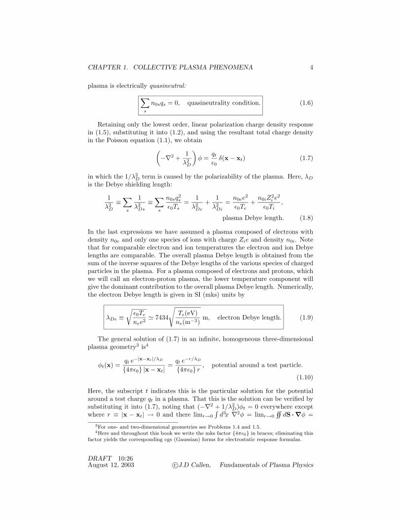
plasma is electrically quasineutral:∑s
n0sqs = 0, quasineutrality condition. (1.6)
Retaining only the lowest order, linear polarization charge density responsein (1.5), substituting it into (1.2), and using the resultant total charge densityin the Poisson equation (1.1), we obtain(
−∇2 +1λ2
D
)φ =
qt
ε0δ(x − xt) (1.7)
in which the 1/λ2D term is caused by the polarizability of the plasma. Here, λD
is the Debye shielding length:
1λ2
D
≡∑
s
1λ2
Ds
≡∑
s
n0sq2s
ε0Ts=
1λ2
De
+1λ2
Di
=n0ee2
ε0Te+
n0iZ2i e2
ε0Ti,
plasma Debye length. (1.8)
In the last expressions we have assumed a plasma composed of electrons withdensity n0e and only one species of ions with charge Zie and density n0i. Notethat for comparable electron and ion temperatures the electron and ion Debyelengths are comparable. The overall plasma Debye length is obtained from thesum of the inverse squares of the Debye lengths of the various species of chargedparticles in the plasma. For a plasma composed of electrons and protons, whichwe will call an electron-proton plasma, the lower temperature component willgive the dominant contribution to the overall plasma Debye length. Numerically,the electron Debye length is given in SI (mks) units by
λDe ≡√ε0Te
nee2$ 7434
√Te(eV)
ne(m−3)m, electron Debye length. (1.9)
The general solution of (1.7) in an infinite, homogeneous three-dimensionalplasma geometry3 is4
φt(x) =qt e−|x−xt|/λD
4πε0 |x − xt| =qt e−r/λD
4πε0 r, potential around a test particle.
(1.10)
Here, the subscript t indicates this is the particular solution for the potentialaround a test charge qt in a plasma. That this is the solution can be verified bysubstituting it into (1.7), noting that (−∇2 + 1/λ2
D)φt = 0 everywhere exceptwhere r ≡ |x − xt| → 0 and there limr→0
∫d3x ∇2φ = limr→0
∫©∫
dS · ∇φ =3For one- and two-dimensional geometries see Problems 1.4 and 1.5.4Here and throughout this book we write the mks factor 4πε0 in braces; eliminating this
factor yields the corresponding cgs (Gaussian) forms for electrostatic response formulas.
DRAFT 10:26August 12, 2003 c©J.D Callen, Fundamentals of Plasma Physics

CHAPTER 1. COLLECTIVE PLASMA PHENOMENA 5
bmin n-1/3
Debye!!!!!!shielding
φCoul
φt
φ
Figure 1.1: Potential φt around a test particle of charge qt in a plasma andCoulomb potential φCoul, both as a function of radial distance from the testparticle. The shaded region represents the Debye shielding effect. The charac-teristic distances are: λD, Debye shielding distance; n−1/3
e , mean electron sep-aration distance; bcl
min = q2/(4πε0T ), classical distance of “closest approach”where the eφ/T << 1 approximation breaks down.
−qt/ε0. The solution given in (1.10) is also the Green function for the equation(−∇2 + 1/λ2
D)φ = ρfree/ε0 — see Problem 1.6.The potential around a test charge in a plasma, (1.10), is graphed in Fig. 1.1.
Close to the test particle (i.e., for r ≡ |x − xt| << λD), the potential is sim-ply the “bare” Coulomb potential φCoul = qt/ (4πε0 |x − xt|) around the testcharge qt. For separation distances of order the Debye length λD, the expo-nential factor in (1.10) becomes significant. For separations large compared tothe Debye length the potential φt becomes exponentially small and hence is“shielded out” by the polarization cloud surrounding the test charge. Overall,there is no net charge Q ≡ ∫V d3x ρq from the combination of the test chargeand its polarization cloud — see Problem 1.7. The difference between φt andthe Coulomb potential is due to the collective Debye shielding effect.
We now use the result obtained in (1.10) to check that the expansion (1.4)was valid. Considering for simplicity a plasma with Ti >> Te [so the electronDebye length dominates in (1.8)], the ratio of the potential around an electrontest charge to the electron temperature at the mean electron separation distanceof |x − xt| = n−1/3
e can be written as
eφt
Te
∣∣∣∣|x−xt|= n−1/3
e
=exp[−1/(neλ3
De
)1/3]
4π (neλ3De)2/3
$ 14π (neλ3
De)2/3. (1.11)
DRAFT 10:26August 12, 2003 c©J.D Callen, Fundamentals of Plasma Physics
CHAPTER 1. COLLECTIVE PLASMA PHENOMENA 6
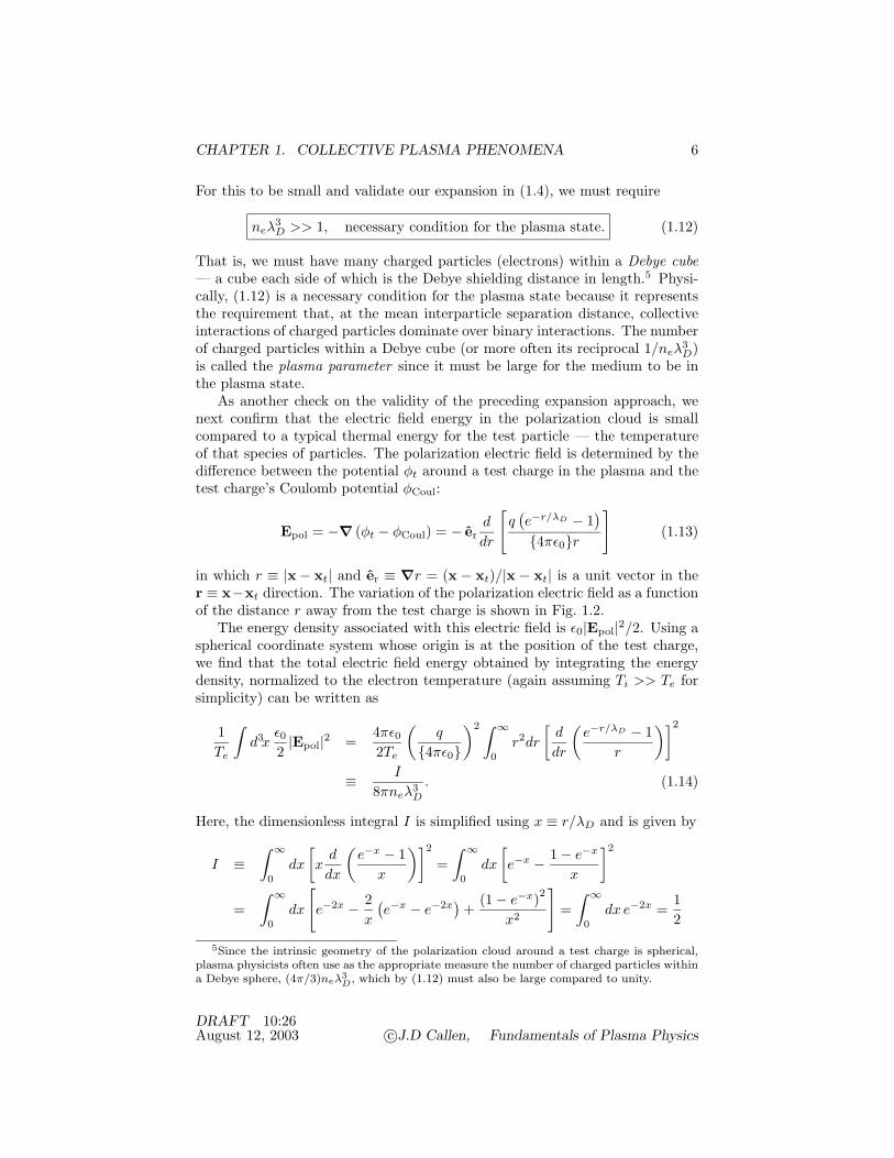
For this to be small and validate our expansion in (1.4), we must require
neλ3D >> 1, necessary condition for the plasma state. (1.12)
That is, we must have many charged particles (electrons) within a Debye cube— a cube each side of which is the Debye shielding distance in length.5 Physi-cally, (1.12) is a necessary condition for the plasma state because it representsthe requirement that, at the mean interparticle separation distance, collectiveinteractions of charged particles dominate over binary interactions. The numberof charged particles within a Debye cube (or more often its reciprocal 1/neλ3
D)is called the plasma parameter since it must be large for the medium to be inthe plasma state.
As another check on the validity of the preceding expansion approach, wenext confirm that the electric field energy in the polarization cloud is smallcompared to a typical thermal energy for the test particle — the temperatureof that species of particles. The polarization electric field is determined by thedifference between the potential φt around a test charge in the plasma and thetest charge’s Coulomb potential φCoul:
Epol = −∇ (φt − φCoul) = − erd
dr
[q(e−r/λD − 1
)4πε0r
](1.13)
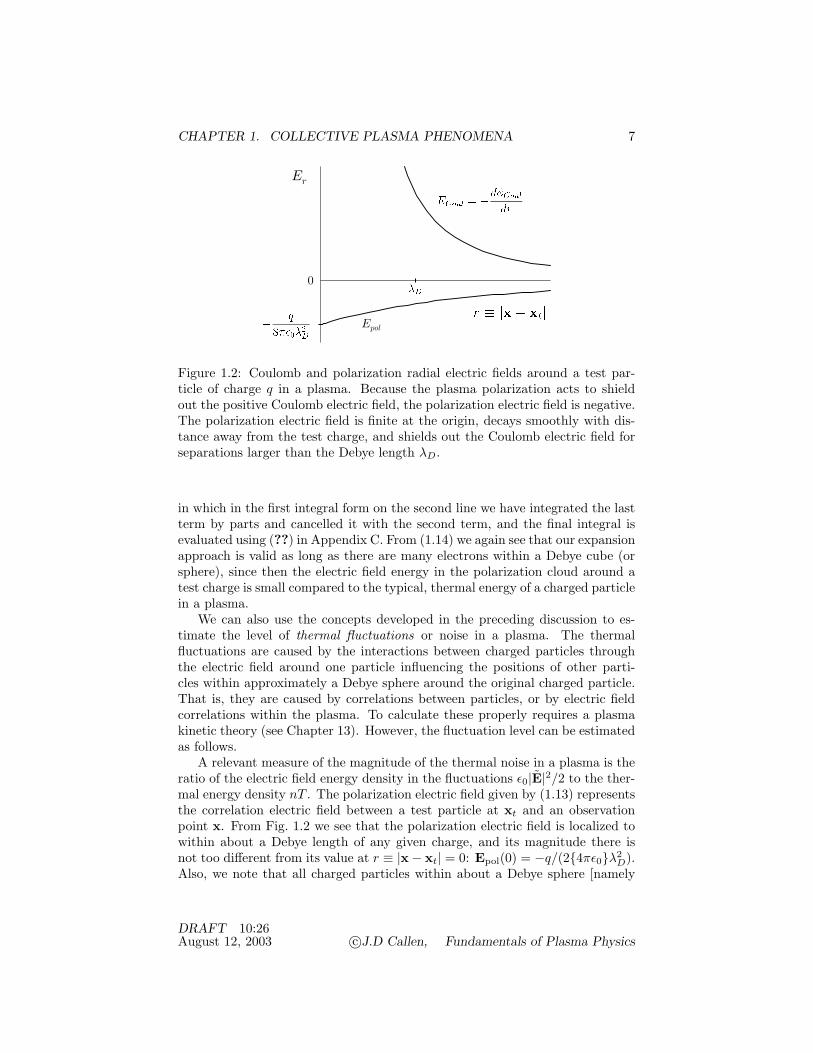
in which r ≡ |x − xt| and er ≡ ∇r = (x − xt)/|x − xt| is a unit vector in ther ≡ x−xt direction. The variation of the polarization electric field as a functionof the distance r away from the test charge is shown in Fig. 1.2.
The energy density associated with this electric field is ε0|Epol|2/2. Using aspherical coordinate system whose origin is at the position of the test charge,we find that the total electric field energy obtained by integrating the energydensity, normalized to the electron temperature (again assuming Ti >> Te forsimplicity) can be written as
1Te
∫d3x
ε02|Epol|2 =
4πε02Te
(q
4πε0)2 ∫ ∞
0r2dr
[d
dr
(e−r/λD − 1
r
)]2≡ I
8πneλ3D
. (1.14)
Here, the dimensionless integral I is simplified using x ≡ r/λD and is given by
I ≡∫ ∞
0dx
[x
d
dx
(e−x − 1
x
)]2=∫ ∞
0dx
[e−x − 1 − e−x
x
]2=∫ ∞
0dx
[e−2x − 2
x
(e−x − e−2x
)+
(1 − e−x)2
x2
]=∫ ∞
0dx e−2x =
12
5Since the intrinsic geometry of the polarization cloud around a test charge is spherical,plasma physicists often use as the appropriate measure the number of charged particles withina Debye sphere, (4π/3)neλ3
D, which by (1.12) must also be large compared to unity.
DRAFT 10:26August 12, 2003 c©J.D Callen, Fundamentals of Plasma Physics
CHAPTER 1. COLLECTIVE PLASMA PHENOMENA 7
Er
Epol
0
Figure 1.2: Coulomb and polarization radial electric fields around a test par-ticle of charge q in a plasma. Because the plasma polarization acts to shieldout the positive Coulomb electric field, the polarization electric field is negative.The polarization electric field is finite at the origin, decays smoothly with dis-tance away from the test charge, and shields out the Coulomb electric field forseparations larger than the Debye length λD.
in which in the first integral form on the second line we have integrated the lastterm by parts and cancelled it with the second term, and the final integral isevaluated using (??) in Appendix C. From (1.14) we again see that our expansionapproach is valid as long as there are many electrons within a Debye cube (orsphere), since then the electric field energy in the polarization cloud around atest charge is small compared to the typical, thermal energy of a charged particlein a plasma.
We can also use the concepts developed in the preceding discussion to es-timate the level of thermal fluctuations or noise in a plasma. The thermalfluctuations are caused by the interactions between charged particles throughthe electric field around one particle influencing the positions of other parti-cles within approximately a Debye sphere around the original charged particle.That is, they are caused by correlations between particles, or by electric fieldcorrelations within the plasma. To calculate these properly requires a plasmakinetic theory (see Chapter 13). However, the fluctuation level can be estimatedas follows.
A relevant measure of the magnitude of the thermal noise in a plasma is theratio of the electric field energy density in the fluctuations ε0|E|2/2 to the ther-mal energy density nT . The polarization electric field given by (1.13) representsthe correlation electric field between a test particle at xt and an observationpoint x. From Fig. 1.2 we see that the polarization electric field is localized towithin about a Debye length of any given charge, and its magnitude there isnot too different from its value at r ≡ |x − xt| = 0: Epol(0) = −q/(24πε0λ2
D).Also, we note that all charged particles within about a Debye sphere [namely
DRAFT 10:26August 12, 2003 c©J.D Callen, Fundamentals of Plasma Physics

CHAPTER 1. COLLECTIVE PLASMA PHENOMENA 8
∼ (4π/3)neλ3D particles] will contribute to the electric field fluctuations at any
given point. Hence, omitting numerical factors, we deduce that the scaling ofthe relative electric field fluctuation energy from “two-particle” correlations ina plasma is given by
ε02|E|2
neTe∼
(4π3
neλ3D
)[ε02|Epol(0)|2
]neTe
∼ 1neλ3
D
<< 1,
thermal fluctuation level. (1.15)
We thus see that, as long as (1.12) is satisfied, the thermal fluctuation level issmall compared to the thermal energy density in the plasma and again our basicexpansion approach is valid. The thermal fluctuations occur predominantly atscale-lengths of order the Debye length or smaller. The appropriate numericalfactor to be used in this formula, and the frequency and wave-number depen-dence of the thermal fluctuations in a plasma, can be obtained from plasmakinetic theory. They will be discussed and determined in Chapter 13.
1.2 Boundary Conditions; Plasma Sheath
A plasma should be larger than the Debye shielding distance in order not tobe dominated by boundary effects. However, at the edge of a plasma whereit comes into contact with a solid material (e.g., a wall, the earth), boundaryeffects become important. The region where the transformation from the plasmastate to the solid state takes place is called the plasma sheath.
The role of a plasma sheath can be understood as follows. First, note thatfor comparable electron and ion temperatures the typical electron speed, whichwill be taken to be the electron thermal speed vTe ≡ √2Te/me [see (??) inSection A.3], is much larger than the typical (thermal) ion speed (vTe/vTi ∼√
mi/me>∼ 43 >> 1). Since the electrons typically move much faster than
the ions,6 electrons tend to leave a plasma much more rapidly than ions. Thiscauses the plasma to become positively charged and build up an equilibriumelectrostatic potential that is large enough [∼ a few Te/e, see (1.23) below]to reduce the electron loss rate to the ion loss rate — so the plasma can bequasineutral in steady state. The potential variation is mostly localized to theplasma sheath region, which is of order a few Debye lengths in width becausethat is the scale length on which significant departures from charge neutralityare allowed in a plasma. Thus, a plasma in contact with a grounded wall will:charge up positively, and be quasineutral throughout most of the plasma, buthave a positively charged plasma sheath region near the wall.
We now make these concepts more concrete and quantitative by estimatingthe properties of a one-dimensional sheath next to a grounded wall using a simpleplasma model. Figure 1.3 shows the specific geometry to be considered along
6Many people use an analogy to remember that electrons have much larger thermal veloc-ities than ions: electrons are like fast moving, lightweight ping pong balls while ions are likeslow-moving, more massive billiard balls — for equal excitation or thermal energies.
DRAFT 10:26August 12, 2003 c©J.D Callen, Fundamentals of Plasma Physics

CHAPTER 1. COLLECTIVE PLASMA PHENOMENA 9
plasmasheath
presheath bulk!plsama
ion!richregion transition quasi-neutral!plasma
φ∞
φs
φ
n
n
0
0
xs
xs
ni
ne
x
x
Figure 1.3: Behavior of the electrostatic potential and electron and ion densitiesin the sheath, presheath (or transition) and bulk plasma regions of a plasmain contact with a grounded wall. For the case shown Te/miV 2∞ = 0.9. Thesheath parameters determined in the text are Φ∞ $ 3 Te/e and xS $ 2λDe.The long-dash line in the top figure indicates the approximation given in (1.26).
with the behavior of the potential, and electron and ion densities in the plasmasheath and bulk plasma regions, as well as in the presheath (or transition) regionbetween them.
The electron density is determined from the Boltzmann relation (1.3):
ne(x) = n∞ exp
e [Φ(x) − Φ∞]Te
(1.16)
in which Φ(x) indicates the equilibrium potential profile in the plasma, and the∞ subscript indicates evaluation of the quantities in the bulk plasma regionfar from the wall (i.e., beyond the plasma sheath and presheath regions whoseproperties we will determine). (In using this equation it is implicitly assumedthat the background electron velocity distribution is Maxwellian.)
For simplicity, we consider an electron-proton plasma with negligible ion
DRAFT 10:26August 12, 2003 c©J.D Callen, Fundamentals of Plasma Physics

CHAPTER 1. COLLECTIVE PLASMA PHENOMENA 10
thermal motion effects (eΦ >> Ti). The potential variation in and near thesheath produces an electric field that increases the flow of ions toward the wall,which will be assumed to be grounded. The ion flow speed Vi in the x directionis governed by conservation of energy for the “cold” (eΦ >> Ti) ions:
12miV
2i (x) + eΦ(x) = constant =
12miV
2∞ + eΦ∞ (1.17)
in which we have allowed for a flow of ions from the bulk of the plasma into thepresheath region so as to ultimately balance the electron flow to the wall. Theion flow at any given point is given by
Vi(x) =√
V 2∞ +2e
mi[Φ∞ − Φ(x)] =
√2e
mi
[Φ∞ +
miV 2∞2e
− Φ(x)].
The spatial change in the ion flow speed causes the ion density to change aswell — a high flow speed produces a low ion density. The ion density variationis governed, in a steady equilibrium, by the continuity or density conservationequation [see (??) in Appendix A] for the ion density: d(niVi)/dx = 0, orni(x)Vi(x) = constant. Thus, referencing the ion density to its value n∞ in thebulk plasma (x → ∞), it can be written as
ni(x) = n∞
1 +2e [Φ∞ − Φ(x)]
miV 2∞
−1/2
. (1.18)
Substituting the electron and ion densities into Poisson’s equation (1.1), weobtain the equation that governs the spatial variation of the potential in thesheath, presheath and plasma regions:
d2Φdx2
= − e
ε0(ni − ne)
= − n∞e
ε0
[1 +
2e [Φ∞ − Φ(x)]miV 2∞
−1/2
− exp− e [Φ∞ − Φ(x)]
Te
].(1.19)
While numerical solutions of this equation can be obtained, no analytic solutionis available. However, limiting forms of the solution can be obtained near thewall (x << xS) and in the bulk plasma (x >> xS). Even though a simplesolution is not available in the transition region, solutions outside this regioncan be used to define the sheath position xS and the conditions needed forproper sheath formation.
In the quasineutral plasma far from the plasma sheath region (x >> xS) thepotential φ(x) is very close to its asymptotic value Φ∞. In this region we approx-imate the electron and ion densities in the limits 2e [Φ∞ − Φ(x)] /miV 2∞<<1 ande [Φ∞ − Φ(x)] /Te<<1, respectively:
ne(x) $ n∞
1 − e [Φ∞ − Φ(x)]Te
+ · · ·
,
ni(x) $ n∞
1 − e [Φ∞ − Φ(x)]miV 2∞
+ · · ·
.
DRAFT 10:26August 12, 2003 c©J.D Callen, Fundamentals of Plasma Physics

CHAPTER 1. COLLECTIVE PLASMA PHENOMENA 11
Keeping only linear terms in Φ∞ − Φ(x), (1.19) can thus be simplified to
d2 [Φ∞ − Φ(x)]dx2
$ 1λ2
De
(1 − Te
miV 2∞
)[Φ∞ − Φ(x)] . (1.20)
Here, λDe is the electron Debye length evaluated at the bulk plasma density n∞.For miV 2∞ < Te the coefficient of Φ∞ − Φ(x) on the right would be negative;this would imply a spatially oscillatory solution that is not physically realis-tic for the present plasma model, which implicitly assumes that the potentialis a monotonic function of x. Thus, a necessary condition for proper sheathformation in this model is
|V∞| ≥√
Te/mi , Bohm sheath criterion. (1.21)
Since this condition need only be satisfied marginally and the ion flow intothe sheath region typically assumes its minimum value, it is usually sufficientto make this criterion an equality. The Bohm sheath criterion implies that ionsmust enter the sheath region sufficiently rapidly to compensate for the electroncharge leakage through the sheath to the wall. In general, what is required forproper sheath formation is that, as we move toward the wall, the local chargedensity increases as the potential decreases: ∂ρq/∂Φ < 0 for all x. Also, sincewe will later find (see Section 1.4) that
√Te/mi is the speed of ion acoustic
waves in a plasma (for the plasma model being considered), the Bohm sheathcriterion implies that the ions must enter the presheath region at a supersonicspeed relative to the ion acoustic speed.
As long as the Bohm sheath criterion is satisfied, solutions of (1.19) will bewell-behaved, and exponentially damped in the presheath region: for x >> xS
we have Φ∞−Φ(x) $ C exp(−x/h) where h = λDe(1−Te/miV 2∞)−1/2 and C isa constant of order Φ∞ − ΦS . Thus, for this plasma model, in the typical casewhere V∞ is equal to or slightly exceeds
√Te/mi, the presheath region where the
potential deviates from Φ∞ extends only a few Debye lengths into the plasma. Inmore comprehensive models for the plasma, and in particular when ion thermaleffects are included, it is found that the presheath region can be larger and thepotential variation in this region is influenced by the effects of sheath geometry,local plasma sources, collisions and a magnetic field (if present). However, theBohm sheath criterion given by (1.21) remains unchanged for most physicallyrelevant situations, as long as the quantity on the right side is interpreted to bethe ion acoustic speed in the plasma model being used.
We next calculate the plasma potential Φ∞ that the plasma will rise to inorder to hold back the electrons so that their loss rate will be equal to the ion lossrate from the plasma. The flux of ions to the wall is given by −niV∞, whichwhen evaluated at the Bohm sheath criterion value given in (1.21) becomes−n∞
√Te/mi. (The flux is negative because it is in the negative x direction.)
A Maxwellian distribution of electrons will produce (see Section A.3) a randomflux of electrons to the wall on the left side of the plasma of −(1/4)neve =−(n∞/4) exp(−eΦ∞/Te)
√8Te/πme. Thus, the net electrical current density to
DRAFT 10:26August 12, 2003 c©J.D Callen, Fundamentals of Plasma Physics
CHAPTER 1. COLLECTIVE PLASMA PHENOMENA 12
the wall will be given by
J = Ji − Je = − e(niV∞ − neve)
= − en∞[√
Te/mi − (1/4)√
8Te/πme exp (−eΦ∞/Te)]. (1.22)
Since in a quasineutral plasma equilibrium we must have J = 0, the plasmapotential Φ∞ is given in this plasma model by
Φ∞ =Te
eln√
mi
2πme≥ 2.84
Te
e$ 3
Te
e, plasma potential, (1.23)
where after the inequality we have used the proton to electron mass ratio mi/me
= 1836. In the original work in this area in 1949, Bohm argued that a potentialdrop of Te/2e extending over a long distance into the plasma (much furtherthan where we are calculating) is required to produce the incoming ion speedV∞ ≥√Te/mi at the sheath edge. In Bohm’s model the density n∞ is e−1/2 =0.61 times smaller than the bulk plasma ion density and thus the ion currentJi is smaller by this same factor. For this model, the potential Φ∞ in (1.23)increases by 0.5 Te/e to 3.34 Te/e. Since lots additional physics (see end ofpreceding paragraph) needs to be included to precisely determine the plasmapotential for a particular situation, and the plasma potential does not changetoo much with these effects, for simplicity we will take the plasma potential Φ∞to be approximately 3Te/e.
Finally, we investigate the form of Φ(x) in the sheath region near the wall(x << xS). In this region the potential is much less than Φ∞ and the electrondensity becomes so small relative to the ion density that it can be neglected. Theequation governing the potential in this ion-rich region can thus be simplifiedfrom (1.19) to
d2Φ(x)dx2
$ − en∞ε0
[miV 2∞/2e
Φ∞ + miV 2∞/2e − Φ(x)
]1/2
. (1.24)
This equation can be de-dimensionalized by multiplying through by e/Te. Thus,defining a dimensionless potential variable χ by
χ(x) ≡ e[Φ∞ + miV 2∞/2e − Φ(x)
]Te
, (1.25)
the equation can be written as
d2χ
dx2$ 1δ2√χ
.
in which δ ≡ λDe/(miV 2∞/2Te)1/4.To integrate this equation we multiply by dχ/dx and integrate over x us-
ing (dχ/dx)(d2χ/dx2) = (1/2)(d/dx)(dχ/dx)2 and dx(dχ/dx)/√χ = dχ/√χ =
2d√χ to obtain
DRAFT 10:26August 12, 2003 c©J.D Callen, Fundamentals of Plasma Physics

CHAPTER 1. COLLECTIVE PLASMA PHENOMENA 13
12
(dχ
dx
)2
$ 2δ2
√χ + constant.
Since both χ and dχ/dx are small near xS , this equation is approximately validfor the x < xS region if we take the constant in it to be zero. Solving theresultant equation for dχ/dx, we obtain
dχ
dx$ − 2χ1/4
δ=⇒ 4
3d(χ3/4) $ − 2dx
δ.
Integrating this equation from x = 0 where χ = χ0 ≡ (eΦ∞ + miV 2∞/2)/Te tox where χ = χ(x), we obtain
χ3/4(x) − χ3/40 $ − 3x
2δ,
or
Φ(x) $ (Φ∞ + miV2∞/2e)[1 − (1 − x/xS)4/3]. (1.26)
Here, we have defined
xS ≡ 2δχ3/40
3=
25/4
3
(Te
miV 2∞
)1/4(eΦ∞ + miV 2∞/2Te
)3/4
λDe,
sheath thickness. (1.27)
Equation (1.26) is valid in the sheath region near the wall (0 < x << xS). Wehave identified the scale length in (1.27) with the sheath width xS because thisis the distance from the wall at which the potential Φ(x) extrapolates to theeffective plasma potential in the bulk plasma, Φ∞ + miV 2∞/2e.
Using the value for Φ∞ given in (1.23) and V∞ $ √Te/mi, the sheaththickness becomes xS $ 2λDe. Thus, as shown in Fig. 1.3, for this model theplasma charges to a positive potential of a few Te/e and is quasineutral upto the non-neutral plasma sheath region, which extends a few Debye lengths(∼ 2 xS ∼ 4λDe in Fig. 1.3) from the grounded wall into the plasma region.
1.3 Langmuir Probe Characteristics*
To further illuminate the electrical properties of a static or equilibrium plasma,we next determine the current that will be drawn out of a probe inserted into aninfinite plasma and biased to a voltage or potential ΦB . Such probes providedsome of the earliest means of diagnosing plasmas and are called Langmuir probes,after Irving Langmuir who developed much of the original understanding oftheir operation. The specific situation to be considered is sketched in Fig. 1.4.For simplicity we assume that the probe is small compared to the size of theplasma and does not significantly disturb it. The probe will be assumed tohave a metallic (e.g., molybdenum) tip and be electrically connected to theoutside world via an insulated tube through the plasma. Probes of this type are
DRAFT 10:26August 12, 2003 c©J.D Callen, Fundamentals of Plasma Physics

CHAPTER 1. COLLECTIVE PLASMA PHENOMENA 14
plasmaISe
I
φI
φp φ
BISiφ
B
Figure 1.4: Schematic of Langmuir probe inserted into a plasma and its idealizedcurrent-voltage characteristics: current I drawn out of the probe as a functionof the bias voltage or potential ΦB . The labeled potentials and currents are:Φf , floating potential; Φp, plasma potential; ISi, ion saturation current; ISe,electron saturation current.
often used in laboratory plasmas that have modest parameters (Te<∼ 10 eV,
ne<∼ 1019 m−3 — probes tend to get burned up at higher plasma parameters).Since the bias potential ΦB on the probe will not affect the incoming ion
flow speed V∞ (for ΦB < Φ∞), following the discussion leading to (1.22) the ioncurrent out of the probe will be given by
Ii = ASJi = −n∞e√
Te/mi AS ≡ −ISi, ion saturation current (ISi), (1.28)
where AS is the area of the probe plus sheath over which the ions are collectedby the probe. For the electrons we must take account of the bias potential ΦB
on the probe. The electron current into the probe is given by
Ie = ApJe =
n∞e√
Te/2πme Ap ≡ ISe, ΦB ≥ Φp,
n∞e√
Te/2πme Ap exp [− e(Φp − ΦB)/Te] , ΦB < Φp,
(1.29)
in which Ap is the area of the probe and Φp is the plasma potential — the voltageat which all electrons heading toward the probe are collected by it. (Whereasthe effective area for ions to be collected by the probe encompasses both theprobe and the sheath, for ΦB < Φp the relevant area Ap for electrons is just theprobe area since only those electrons surmounting the sheath potential makeit to the probe — see Fig. 1.3. However, when ΦB > Φp the relevant area,and consequent electron current, grows slightly and roughly linearly with bias
DRAFT 10:26August 12, 2003 c©J.D Callen, Fundamentals of Plasma Physics

CHAPTER 1. COLLECTIVE PLASMA PHENOMENA 15
voltage, which is then attracting electrons and modifying their trajectories inthe vicinity of the probe. In the idealized current-voltage curve in Fig. 1.4 wehave neglected this latter effect.)
The total current I = Ii + Ie drawn to the probe is shown in Fig. 1.4as a function of the bias voltage or potential ΦB . For a large negative biasthe electron current becomes negligible and the current is totally given by theion current ISi, which is called the ion saturation current. The potential Φf
at which the current from the probe vanishes is called the floating potential ,which is zero for our simple model. However, it is often slightly negative in realplasmas, unless there is secondary electron emission from the probe, in whichcase it can become positive. For potentials larger than the plasma potentialΦp all electrons on trajectories that intercept the probe are collected and thecurrent is given by the electron saturation current ISe. Except for differencesin the charged particle collection geometry (typically cylindrical or sphericalprobes versus a planar wall), in the sheath thickness (relative to probe size)effects and perhaps in secondary electron emission, the difference between theplasma and floating potentials is just the naturally positive plasma potentialthat we derived in (1.23). That is, Φp − Φf $ Φ∞ ∼ 3 Te/e.
In a real plasma the idealized current-voltage characteristic that is indicatedin Fig. 1.4 gets rounded off and distorted somewhat due to effects such as chargedparticle orbit effects in the sheath, probe geometry, secondary electron emissionfrom the probe and other effects. Indeed, because of the practical importance ofLangmuir probes in measuring plasma parameters in many laboratory plasmas,as we will discuss in the next paragraph, there is a large literature on thecurrent-voltage characteristics of various types of probes in real plasmas (seereferences and suggested reading at the end of the chapter). Nonetheless, thebasic characteristics are as indicated in Fig. 1.4.
For bias potentials that lie between the floating and plasma potentials, thecurrent from the probe increases exponentially with bias potential ΦB . Thus,the electron temperature can be deduced from the rate of exponential growth inthe current as the bias potential is increased: Te/e $(I − ISi)/(dI/dΦB). Alter-natively, one can use a “double probe” to determine the electron temperature —see Problem 1.11. If the electron temperature is known, the plasma ion densitycan be estimated from the ion saturation current: n∞ $ ISi/(eAS
√Te/Mi).
Langmuir probes are thus important diagnostics for measuring the plasma den-sity and electron temperature in laboratory plasmas with modest parameters.
The thickness of the plasma sheath changes as the bias potential ΦB isvaried. The derivation of the sheath thickness xS given in (1.24) to (1.27) canbe modified to account for the present biased probe situation by replacing thepotential Φ∞ with Φp − ΦB . Thus, setting miV 2∞/Te to unity to satisfy theBohm sheath criterion (1.21), the sheath thickness around a biased probe in aplasma is given approximately by
xS $ 25/4
3
(Φp + 0.5 − ΦB
Te/e
)3/4
λDe, sheath thickness. (1.30)
DRAFT 10:26August 12, 2003 c©J.D Callen, Fundamentals of Plasma Physics

CHAPTER 1. COLLECTIVE PLASMA PHENOMENA 16
This formula is valid for e(Φp+0.5−ΦB) >> Te — small or negative bias voltagesΦB − Φp. As the bias potential ΦB increases toward the plasma potential Φp,the plasma sheath becomes thinner; it disappears for e(Φp − ΦB) <∼ 0.5 Te.
For large negative bias potentials (|ΦB | >> Te/e), the electrical currentdensity flowing through the ion-rich sheath region is limited by “space charge”effects and given by the Child-Langmuir law — see Problem 1.13. However, tran-siently the current density can be larger that indicated by the Child-Langmuirlaw — see Problem 1.14.
1.4 Inertial Response; Plasma Oscillations
In the preceding sections on Debye shielding and its effects we considered theadiabatic or static response of charged particles and a plasma to the Coulombelectric field around a charged particle in the plasma. Next, we discuss theinertial (or dynamic) response of a plasma. To do this we consider the electricpolarization response of charged particles and a plasma to a small electric fieldperturbation, which may be externally imposed or be collectively generatedwithin the plasma.
First, we calculate the motion of a charged particle in response to an electricfield. The velocity v of a charged particle of mass m and charge q subjectedto an electric field perturbation7 E(x, t) is governed by Newton’s second law(F = ma) with force qE:
mdvdt
= q E(x, t). (1.31)
The electric field perturbation will be assumed to be small enough and suffi-ciently slowly varying in space so that nonlinear and translational motion effectsare negligible. Thus, it will be sufficient to evaluate the electric field at the ini-tial position x0 and neglect the small variation in the electric field induced bythe motion x(t) of the charged particle. This approximation will be discussedfurther after the next paragraph.
Integrating (1.31) over time, the velocity perturbation v(t) induced by theelectric field perturbation for a particle with initial velocity v0 is given by
v(t) ≡ v(t) − v0 =q
m
∫ t
0dt′ E[x′(t′), t′] $ q
m
∫ t
0dt′ E(x0, t
′). (1.32)
Integrating once more over time, we find that the motion induced by the electricfield perturbation becomes
x(t) ≡ x(t) − (x0 + v0t) $ q
m
∫ t
0dt′∫ t′
0dt′′ E(x0, t
′′), inertial response.
(1.33)7Perturbations to an equilibrium will be indicated throughout the book by a tilde over
the symbol for the perturbed quantity. Equilibrium quantities will be indicated by 0 (zero)subscripts.
DRAFT 10:26August 12, 2003 c©J.D Callen, Fundamentals of Plasma Physics

CHAPTER 1. COLLECTIVE PLASMA PHENOMENA 17
Because the response of the particle to the electric field force is limited by theinertial force ma = m dv/dt, this is called an inertial response. Note that thisresponse is inversely proportional to the mass of the charged particle; thus,the lighter electrons will give the primary inertial response to an electric fieldperturbation in a plasma.
We check our approximation of evaluating the electric field at the initialposition x0 by expanding the electric field in a Taylor series expansion aboutthe charged particle trajectory given by
E [x(t), t] = E (x0, t) + (x + v0t) · ∇E |x0 + · · · (1.34)
Our approximation is valid as long as the second (and higher order) terms inthis expansion are small compared to the first term:
(x + v0t) · ∇E << E. (1.35)
Thus, the electric field perturbation must vary sufficiently slowly in space (i.e.,the gradient scale length |(1/|E|)∇E|−1 must be long compared to the distance|x + v0t|), be small enough (so the nonlinear term x · ∇E is small compared toE) and the elapsed time must not be too long. These approximations will bechecked a posteriori — at the end of this section.
The inertial motion x of a charged particle in response to the electric fieldperturbation creates an electric dipole moment qx. A uniform density n0 of suchcharged particles leads to an electric polarization density P = n0qx. Summingover the species of charged particles in the plasma, the total plasma polarizationdensity becomes
P =∑
s
n0sqsxs = ε0∑
s
ω2ps
∫ t
0dt′∫ t′
0dt′′ E (t′′) (1.36)
in which for each charged species s
ω2ps ≡ n0sq2
s
msε0, square of species plasma frequency, (1.37)
is the inertial or plasma frequency for a species s, whose physical significancewill be discussed below.
Because the ions are so much more massive than the electrons (the ratio ofthe proton to electron mass is 1836), they have much more inertia. Thus, theirplasma frequency is much smaller than that for the electrons — for example,for protons ωpi/ωpe =
√me/mp $ 1/43 << 1. Since the electrons give the
dominant contribution to the plasma polarization and have the largest plasmafrequency, we have ∑
s
ω2ps = ω2
pe + ω2pi $ ω2
pe. (1.38)
DRAFT 10:26August 12, 2003 c©J.D Callen, Fundamentals of Plasma Physics

CHAPTER 1. COLLECTIVE PLASMA PHENOMENA 18
Numerically, the electron plasma frequency is given by
ωpe ≡√
nee2
meε0$ 56
√ne(m−3) rad/sec, radian plasma frequency, (1.39)
or
fpe ≡ ωpe/2π $ 9√
ne(m−3) Hz, plasma frequency. (1.40)
The plasma polarization in (1.36) causes [see(??) and (??) Section A.2] a po-larization charge density ρpol given by the negative of the divergence of thepolarization P:
ρpol(E) = −∇· P = − ε0∑
s
ω2ps
∫ t
0dt′∫ t′
0dt′′ ∇· E(t′′). (1.41)
Now, to calculate the perturbed electric field E in a plasma we need to useGauss’s law, which is given in (1.1). For the charge density ρq we imagine thatthere are polarization charge densities due to both the electric field perturbationwe have been considering, and an externally imposed electric field Eext whichsatisfies the same conditions as E — namely condition (1.35). Thus, the relevantform of Gauss’s law becomes
∇· E =1ε0ρpol = −
∑s
ω2ps
∫ t
0dt′∫ t′
0dt′′ ∇ ·
[E(t′′) + Eext(t′′)
]. (1.42)
This differential and integral equation in space and time, respectively, can bereduced to a simpler, completely differential form by taking its second partialderivative with respect to time to yield
∇ ·[∂2E∂t2
+∑
s
ω2ps
(E + Eext
)]= 0. (1.43)
Using the approximation in (1.38), we thus find that taking into account theinertial effects of charged particles (mostly electrons), nontrivial (i.e., nonvan-ishing) electric field perturbations satisfying condition (1.35) are governed bythe differential equation
∂2E∂t2
+ ω2peE = −ω2
peEext. (1.44)
This is a linear, inhomogeneous differential equation of the harmonic oscilla-tor type with frequency ωpe for the perturbed electric field E induced by theexternally applied electric field Eext.
The “complementary” (in the current langauge of mathematics) solutions ofthe homogeneous part of this equation are of the form
Eh = Cc cosωpet + Cs sinωpet, (1.45)
DRAFT 10:26August 12, 2003 c©J.D Callen, Fundamentals of Plasma Physics
CHAPTER 1. COLLECTIVE PLASMA PHENOMENA 19
L
plasma
V(t)
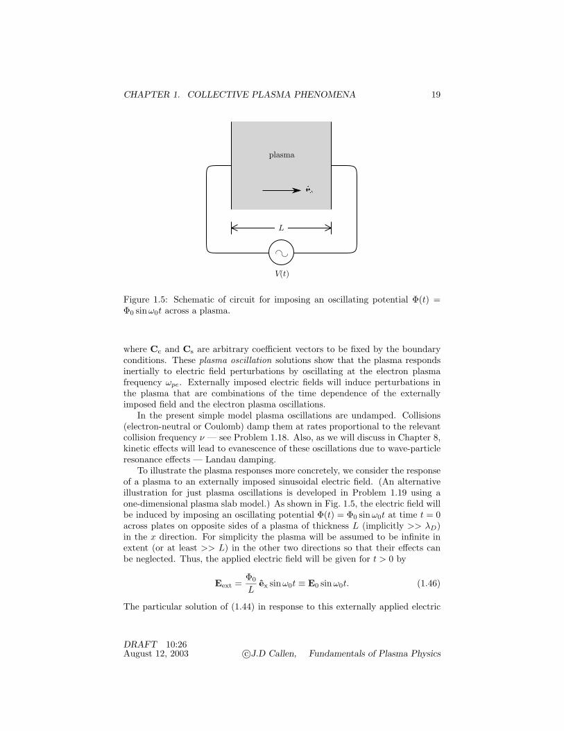
Figure 1.5: Schematic of circuit for imposing an oscillating potential Φ(t) =Φ0 sinω0t across a plasma.
where Cc and Cs are arbitrary coefficient vectors to be fixed by the boundaryconditions. These plasma oscillation solutions show that the plasma respondsinertially to electric field perturbations by oscillating at the electron plasmafrequency ωpe. Externally imposed electric fields will induce perturbations inthe plasma that are combinations of the time dependence of the externallyimposed field and the electron plasma oscillations.
In the present simple model plasma oscillations are undamped. Collisions(electron-neutral or Coulomb) damp them at rates proportional to the relevantcollision frequency ν — see Problem 1.18. Also, as we will discuss in Chapter 8,kinetic effects will lead to evanescence of these oscillations due to wave-particleresonance effects — Landau damping.
To illustrate the plasma responses more concretely, we consider the responseof a plasma to an externally imposed sinusoidal electric field. (An alternativeillustration for just plasma oscillations is developed in Problem 1.19 using aone-dimensional plasma slab model.) As shown in Fig. 1.5, the electric field willbe induced by imposing an oscillating potential Φ(t) = Φ0 sinω0t at time t = 0across plates on opposite sides of a plasma of thickness L (implicitly >> λD)in the x direction. For simplicity the plasma will be assumed to be infinite inextent (or at least >> L) in the other two directions so that their effects canbe neglected. Thus, the applied electric field will be given for t > 0 by
Eext =Φ0
Lex sinω0t ≡ E0 sinω0t. (1.46)
The particular solution of (1.44) in response to this externally applied electric
DRAFT 10:26August 12, 2003 c©J.D Callen, Fundamentals of Plasma Physics

CHAPTER 1. COLLECTIVE PLASMA PHENOMENA 20
field is
Ep =ω2
pe
ω20 − ω2
pe
E0 sinω0t. (1.47)
Adding together the homogeneous, particular and externally applied electricfield components (E = E+Eext = Eh + Ep +Eext) of the solution of (1.44), andsubjecting them to the boundary conditions that E(t = 0) = 0 and dE/dt |t=0
= dEext/dt |t=0 = ω0E0, we find Cc = 0 and Cs = − [ω0ωpe/(ω2
0 − ω2pe
)]E0.
Hence, the total electric field E driven by Eext is given for t > 0 by
E(t) =ω0ωpe
ω20 − ω2
pe
E0 sinωpet +ω2
pe
ω20 − ω2
pe
E0 sinω0t + E0 sinω0t
= − ω0ωpe
ω20 − ω2
pe
E0 sinωpet +ω2
0
ω20 − ω2
pe
E0 sinω0t
≡ Eplasma sinωpet + Edriven sinω0t. (1.48)
The frequency dependences of the net driven response Edriven oscillating atfrequency ω0 and of the response Eplasma oscillating at the plasma frequencyωpe are shown in Fig. 1.6. For ω0 much less than the electron inertial or plasmafrequency ωpe, we find that Edriven is of order −ω2
0/ω2pe compared with the
externally applied electric field E0 sinω0t, and hence tends to be small. Inthis limit the electrons have little inertia (ω0 << ωpe) and they develop astrong polarization response that tends to collectively shield out the externallyapplied electric field from the bulk of the plasma. In the opposite limit ω2
0 >>ω2
pe, the inertia of the electrons prevents them from responding significantly,their polarization response is small, and the externally imposed electric fieldpermeates the plasma — in this limit E $ Eext since E << Eext. The singularityat ω0 = ωpe indicates that when the driving frequency ω0 coincides with thenatural plasma oscillation frequency ωpe the linear response is unbounded. InChapters 7 and 8 we will see that collisions or kinetic effects bound this responseand lead to weak damping effects for ω0 $ ωpe. Nonlinear effects can also leadto bounds on this response.
The Eplasma response in (1.48), which oscillates at the plasma frequency, iscaused by the electron inertia effects during the initial turn-on of the externalelectric field. Note that it vanishes in both the low and high frequency limits —because for low ω0 the excitation is small for the nearly adiabatic (ω0 << ωpe)turn-on phase, while for high ω0 the electron inertial response is small during thevery brief (δt ∼ 1/ω0 << 1/ωpe) turn-on phase. Like the driven response, theplasma response becomes unbounded in this simple plasma model for ω0 → ωpe.
Finally, we go back and determine the conditions under which the approxi-mation (1.35) that we made in calculating the plasma polarization induced byan electric field is valid. Referring to the physical situation shown in Fig. 1.5, wetake the gradient scale length of the electric field perturbation |(1/|E|)∇E|−1
to be of order the spacing L between the plates. We first estimate the conditionimposed by the particle streaming indicated by the term v0t in (1.35). To make
DRAFT 10:26August 12, 2003 c©J.D Callen, Fundamentals of Plasma Physics

CHAPTER 1. COLLECTIVE PLASMA PHENOMENA 21
0
collectiveshielding
dielectricmedium
wpe w
E0
Figure 1.6: Frequency dependence of the electric field components oscillat-ing at the driven frequency ω0 (Edriven, solid lines) and the plasma frequencyωpe(Eplasma, dashed lines) induced in a plasma by Eext = E0 sinω0t, as indi-cated in Fig. 1.5. The driven frequency response is shielded out for ω0 << ωpe;it approaches the imposed electric field for ω0 >> ωpe. The plasma frequencyresponse is induced by the process of turning on the external electric field; itbecomes small when ω0 is very different from ωpe. The singular behavior forω0 → ωpe results from driving the system at the natural oscillation frequency ofthe plasma, the plasma frequency; it is limited in more complete plasma modelsby collisional, kinetic or nonlinear effects.
this estimate we take v0 to be of order the most probable electron thermal speedvTe ≡√2Te/me [see (??) in Section A.3]. Also, we estimate t by 1/ω. However,since the most important plasma effects occur for ω ∼ ωpe (see Fig. 1.6), wescale ω to ωpe. Then, since vTe/ωpe =
√2λDe, the particle streaming part of
(1.35) leads, neglecting numerical factors, to the condition
L >> λDe (ωpe/ω) . (1.49)
That is, for ω ∼ ωpe the plasma must be large compared to the electron Debyelength.
For validity of the nonlinear condition x · ∇E << E we consider a situationwhere E = (Φ/L) sinωt. Then, again neglecting numerical factors, we find thatto neglect the nonlinearities we must require
eΦTe
<<L2
λ2De
(ω2
ω2pe
). (1.50)
Since we can anticipate from physical considerations that potential fluctuationsΦ are at most of order some modest factor times the electron temperature in aplasma, the nonlinear criterion is usually well satisfied as long as the streaming
DRAFT 10:26August 12, 2003 c©J.D Callen, Fundamentals of Plasma Physics
CHAPTER 1. COLLECTIVE PLASMA PHENOMENA 22
criterion in (1.49) is. Hence, our derivation of the plasma polarization is gen-erally valid for ω ∼ ωpe plasma oscillation phenomena as long as the plasmaunder consideration is much larger than the electron Debye length.
We can also use the preceding logic to specify the temporal and spatialscales on which the inertial response and effects discussed in this section applyin an infinite, homogeneous plasma — versus the conditions where the adiabaticresponse in the first section of this chapter apply. (For a general discussion ofinertial and adiabatic responses — for a harmonic oscillator — see Appendix E.)For ω ∼ ωpe, as long as the scale length L ∼ δx of interest is long compared to theelectron Debye length λDe, conditions (1.35), (1.49) and (1.50) are all satisfied.Then, the inertial and electron plasma oscillation effects we have discussed arerelevant since ω >> vTe/δx, which is the inverse of the time required for athermal electron to move a distance δx. However, for low frequencies ω << ωpe
such that δx << λDe(ω/ωpe), or for scale lengths δx << λDe with ω ∼ ωpe, theinequality conditions become reversed and the approximations we have usedin this section break down. Then, instead of an inertial response, we obtainan adiabatic response for ω << vTe/δx and the Debye shielding effects wediscussed in the first section of this chapter. Intermediate situations with δx ∼λDe(ωpe/ω) ∼ vTe/ω must be treated kinetically — see Chapter 8.
1.5 Plasma as a Dielectric Medium
In general, any vector field such as the electric field perturbation E is com-posed of both longitudinal (irrotational, ∇· E ,= 0) and transverse (solenoidal,∇· E = 0) parts — see Section D.5 of Appendix D. From the form of (1.43) itis clear that we have been discussing the longitudinal component of the electricfield perturbation. This component is derivable from a potential, E = −∇φ,and represents the electrostatic component of the electric field perturbation.Since we have ∇· E = −∇2φ ,= 0, we see from Gauss’s law (1.1) that these elec-trostatic perturbation components correspond to charge density perturbationsin the plasma. Thus, the electron plasma oscillations we have been discussingare electrostatic “space charge” oscillations in which the longitudinal componentof the electric field and plasma polarization oscillate out of phase with respectto each other, i.e., ∂2(∇· E)/∂t2 = −ω2
pe∇· E = − ∂2(∇· P)/∂t2.The polarizability of the plasma by an electric field perturbation can also be
interpreted by considering the plasma to be a dielectric medium. To illustratethis viewpoint, we note that in a dielectric medium Gauss’s law becomes [see(??) in Section A.2]
∇· D = ρfree, (1.51)
where
D ≡ εE (1.52)
is the displacement vector, ρfree is the charge density of the free charges (i.e.,those not contributing to the plasma dielectric), and ε is the dielectric constant of
DRAFT 10:26August 12, 2003 c©J.D Callen, Fundamentals of Plasma Physics
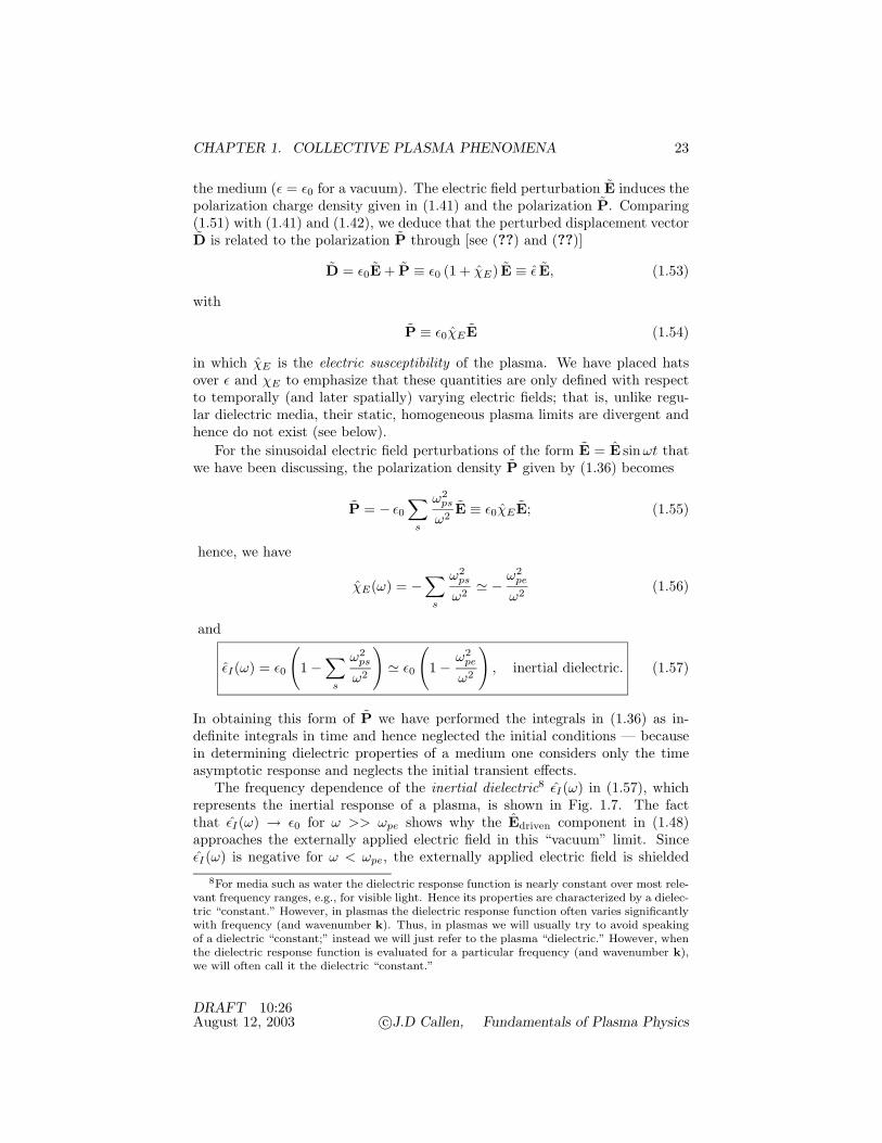
CHAPTER 1. COLLECTIVE PLASMA PHENOMENA 23
the medium (ε = ε0 for a vacuum). The electric field perturbation E induces thepolarization charge density given in (1.41) and the polarization P. Comparing(1.51) with (1.41) and (1.42), we deduce that the perturbed displacement vectorD is related to the polarization P through [see (??) and (??)]
D = ε0E + P ≡ ε0 (1 + χE) E ≡ ε E, (1.53)
with
P ≡ ε0χEE (1.54)
in which χE is the electric susceptibility of the plasma. We have placed hatsover ε and χE to emphasize that these quantities are only defined with respectto temporally (and later spatially) varying electric fields; that is, unlike regu-lar dielectric media, their static, homogeneous plasma limits are divergent andhence do not exist (see below).
For the sinusoidal electric field perturbations of the form E = E sinωt thatwe have been discussing, the polarization density P given by (1.36) becomes
P = − ε0∑
s
ω2ps
ω2E ≡ ε0χEE; (1.55)
hence, we have
χE(ω) = −∑
s
ω2ps
ω2$ − ω2
pe
ω2(1.56)
and
εI(ω) = ε0
(1 −∑
s
ω2ps
ω2
)$ ε0
(1 − ω2
pe
ω2
), inertial dielectric. (1.57)
In obtaining this form of P we have performed the integrals in (1.36) as in-definite integrals in time and hence neglected the initial conditions — becausein determining dielectric properties of a medium one considers only the timeasymptotic response and neglects the initial transient effects.
The frequency dependence of the inertial dielectric8 εI(ω) in (1.57), whichrepresents the inertial response of a plasma, is shown in Fig. 1.7. The factthat εI(ω) → ε0 for ω >> ωpe shows why the Edriven component in (1.48)approaches the externally applied electric field in this “vacuum” limit. SinceεI(ω) is negative for ω < ωpe, the externally applied electric field is shielded
8For media such as water the dielectric response function is nearly constant over most rele-vant frequency ranges, e.g., for visible light. Hence its properties are characterized by a dielec-tric “constant.” However, in plasmas the dielectric response function often varies significantlywith frequency (and wavenumber k). Thus, in plasmas we will usually try to avoid speakingof a dielectric “constant;” instead we will just refer to the plasma “dielectric.” However, whenthe dielectric response function is evaluated for a particular frequency (and wavenumber k),we will often call it the dielectric “constant.”
DRAFT 10:26August 12, 2003 c©J.D Callen, Fundamentals of Plasma Physics

CHAPTER 1. COLLECTIVE PLASMA PHENOMENA 24
wwpe
ε0
0
Figure 1.7: Frequency dependence of inertial response plasma dielectric.
out of the plasma or “cut off” in this frequency range. The vanishing of εI forω = ωpe indicates that this is a “normal mode” of oscillation of the plasma, asis evident from the plasma oscillator equation (1.44) — driven electric fields atfrequencies where the dielectric vanishes lead to unbounded resonant responsesin linear theory, as can be inferred from (1.51) and (1.52). Also, since εI is smallfor ω close to ωpe, the transient plasma frequency response Eplasma is largestin this frequency range. Finally, we note that εI(ω) is divergent in the ω → 0or static limit. Thus, the inertial dielectric response of a plasma can only bedefined for temporally varying processes.
Because the polarization of the plasma is 180 out of phase with respectto the electric field perturbations for all real ω, the inertial plasma response isreactive (i.e., not dissipative) for all frequencies ω. That there is no dissipationcan be demonstrated explicitly by calculating the average Joule heating E · Jwith J = n0ev over an oscillation period 2π/ω and showing that it vanishes.If dissipative effects, such as collisons, are added, they lead to wave dampingthrough the joule heating they induce in the plasma — see Problem 1.18
The energy density of plasma oscillations is composed of two parts: thevacuum electric field energy density ε0|E|2/2 and the polarization energy den-sity wpol = − 1
2 P · E = − 12ε0χE |E|2. For an electric field perturbation E
oscillating at frequency ω the polarization is given in (1.55). Thus, we findwpol = (ε0/2)(ω2
pe/ω2)|E|2. Hence, the total energy density [see (??)] in an
electrostatic plasma oscillation is given by
wE ≡ 12(E · D) =
ε02|E|2 + wpol =
ε02
(1 +
ω2pe
ω2
)|E|2, wave energy density.
(1.58)
For low frequencies (ω << ωpe), for which an externally imposed electricfield is shielded out of the plasma, the polarization energy density is dominant.
DRAFT 10:26August 12, 2003 c©J.D Callen, Fundamentals of Plasma Physics
CHAPTER 1. COLLECTIVE PLASMA PHENOMENA 25
In contrast, for high frequencies (ω >> ωpe) the electron inertia effects causethe polarization to be small; then, the energy density is predominantly just thatresiding in the electric field perturbation itself. The fact that the energy densitycaused by electric field perturbations can have a significant (or even dominant,as occurs for ω << ωpe) component due to the polarizability of the plasma is avery important aspect of plasma oscillations.
1.6 Ion Acoustic Waves
In the preceding sections we have implicitly assumed that the electrons andions both exhibit either adiabatic or inertial responses. However, because theions are much heavier, they have a much lower inertial or plasma frequencyand, for the typical case where Te ∼ Ti, a much lower thermal speed thanelectrons. Thus, for a given length scale δx there is an intermediate frequencyregime vTi/δx << ω << vTe/δx in which the ions respond inertially while theelectrons respond adiabatically. We will now determine the equation governingelectric field perturbations in a plasma in this regime.
The perturbed electron density for an adiabatic (ω << vTe/δx) responseinduced by a potential perturbation φ of a quasineutral plasma equilibrium(∑
s n0sqs = 0) is obtained from the perturbed Boltzmann relation (1.4):
ne = n0eeφ
Te. (1.59)
The perturbed ion density for an inertial (ω >> vTi/δx) response induced byan electric field perturbation E is obtained from the ion polarization part of thetotal plasma charge density given in (1.41):
ni = − ε0qiω2
pi
∫ t
0dt′∫ t′
0dt′′ ∇· E(t′′). (1.60)
The overall perturbed charge density in this intermediate frequency regime isthus given by
ρq
ε0=∑
s
nsqs
ε0= − ω2
pi
∫ t
0dt′∫ t′
0dt′′ ∇· E(t′′) − n0ee2
ε0Teφ
= + ω2pi
∫ t
0dt′∫ t′
0dt′′ ∇2φ(t′′) − φ
λ2De
(1.61)
in which we have specialized to electrostatic perturbations for which E = −∇φand ∇· E = −∇2φ.
Substituting this perturbed charge density into Poisson’s equation (1.1), weobtain
−(∇2 − 1
λ2De
)φ = ω2
pi
∫ t
0dt′∫ t′
0dt′′ ∇2φ(t′′).
DRAFT 10:26August 12, 2003 c©J.D Callen, Fundamentals of Plasma Physics

CHAPTER 1. COLLECTIVE PLASMA PHENOMENA 26
Or, taking the second partial derivative with respect to time, this yields
−(∇2 − 1
λ2De
)∂2φ
∂t2= ω2
pi∇2φ. (1.62)
Considering perturbations whose scale lengths are long compared to the electronDebye length
(∇2 << 1/λ2De
), the equation governing potential perturbations
in the intermediate frequency regime becomes simply
∂2φ
∂t2− c2
S∇2φ = 0, ion acoustic wave equation, (1.63)
in which
c2S = ω2
pi λ2De =
Te
mi
niq2i
neq2e
=ZiTe
mi. (1.64)
As indicated in the last equality, for a plasma with a single ion componentniq2
i = Zinee2 so that c2S = ZiTe/mi. The quantity cS has the units of a speed
and as we will see below is the speed of ion acoustic (or sound) waves in aplasma. It is given numerically by
cS ≡√
ZiTe
mi$ 104
√ZiTe(eV)
Aim/s, ion acoustic speed, (1.65)
in which Ai is the atomic mass of the ions in the plasma: Ai ≡ mi/mp. Here,we have used the subscript S on c to indicate that these ion acoustic wavesare the natural “sound” (S) waves that occur in a plasma. The relation of ionacoustic waves to normal sound waves in a neutral gas are discussed at the lastof this section, and their relation to the sound waves in a magnetohydrodynamicdescription of a plasma is discussed in Section 7.2.
Equation (1.63) is a wave equation. In one dimension, say the x direction,general solutions of it are given by a linear combination of arbitrary functionsf1, f2 of its mathematical characteristics ϕ± ≡ x ∓ cSt:
φ(x, t) = C1f1(x − cSt) + C2f2(x + cSt),
where C1 and C2 are arbitrary constants to be fixed by the boundary conditions.A point of constant phase in this solution moves at the phase speed Vϕ of thewave: dϕ± = 0 = dx ∓ cSdt =⇒ Vϕ = dx/dt = ±cS along the mathematicalcharacteristics x = x0 ± cSt.
For wave-like equations such as those in (1.62) or (1.63) we usually seeksolutions of the form
φ (x, t) = φ ei(k·x−ωt) (1.66)
in which φ is a constant, k is the (vector) wavenumber and ω is the frequencyof the wave. Substituting this Ansatz (proposed form) into (1.62), we find[− (−k2 − 1/λ2
De
) (−ω2)
+ ω2pik
2]φ = 0.
DRAFT 10:26August 12, 2003 c©J.D Callen, Fundamentals of Plasma Physics

CHAPTER 1. COLLECTIVE PLASMA PHENOMENA 27
k
w
wpi
Figure 1.8: Dispersion diagram for ion acoustic waves in an electron-protonplasma with Te >> Ti. For kλDi << 1 the ion acoustic waves propagate atthe ion acoustic speed: ω/k $ cS . The dispersion curve ω = ω(k) is shown asa dashed line for kλDi
>∼ 1 because in this region the ion response is no longerinertial (kinetic effects become important) and the present analysis becomesinvalid.
For nontrivial solutions with φ ,= 0, we must have
ω2 =k2c2
S
1 + k2λ2De
=ω2
pi
1 + 1/ (k2λ2De)
, ion acoustic wave dispersion relation.
(1.67)
This is called a dispersion relation because it givess the dependence of ω on k— here for electrostatic ion acoustic waves propagating in a plasma.
The dispersion diagram (ω versus k) for ion acoustic waves is shown inFig. 1.8. For k2λ2
De << 1 (long scale lengths compared to the electron Debyelength) we have ω/k = ±cS — the phase speed Vϕ ≡ ω/k of the wave is theion acoustic speed cS . Since we have assumed that the ions have an inertialresponse, taking δx ∼ 1/k we must have vTi/δx ∼ kvTi << ω $ kcs. Thiscondition is satisfied and ion acoustic waves exist in an electron-proton plasmaonly if the ion acoustic speed cS ≡√Te/mi is much larger than the ion thermalspeed vTi =
√2Ti/mi, which occurs only if Te >> 2Ti. As can be discerned
from (1.67), the wave frequency ω increases for increasing kλDe and asymptotesto ωpi for kλDe >> 1. However, to satisfy the required condition for an ioninertial response we must have kvTi << ω ∼ ωpi or kλDi << 1. We can satisfykλDe >> 1 >> kλDi only if Te >> Ti, which is the same as the condition notedpreviously in this paragraph for the existence of ion acoustic waves.
As we discussed in the preceeding section, plasma responses can also bedescribed terms of the plasma giving a dielectric response ε. For waves of the
DRAFT 10:26August 12, 2003 c©J.D Callen, Fundamentals of Plasma Physics
CHAPTER 1. COLLECTIVE PLASMA PHENOMENA 28
form given in (1.66) the polarization corresponding to the perturbed chargedensity in (1.61) becomes
P = ε0
(−ω
2pi
ω2+
1k2λ2
De
)E, (1.68)
in which we have used E = −ikφ and ∇· E = −∇2φ = k2φ. Using the defini-tions for the interrelationships between P, χE and ε given in (1.53), (1.54), wefind that in the intermediate frequency regime we are considering the plasmadielectric response is given by
εS (k,ω) = ε0
(1 − ω2
pi
ω2+
1k2λ2
De
), ion acoustic dielectric. (1.69)
Setting this εS to zero to obtain the normal modes of the plasma readilyyields the dispersion relation for ion acoustic waves given in (1.67). This di-electric function diverges for either ω → 0 or k → 0. Thus, again, the plasmadielectric is only a meaningful quantity for temporal and spatially varying per-turbations, i.e., not for an infinite, homogeneous equilibrium. Also, since εSis real for all real k,ω (i.e.,the electron and ion components of the polariza-tion are in phase or 180 out of phase with the electric field perturbation), thisintermediate frequency response is also totally reactive (i.e., not dissipative).
Ion acoustic waves are similar to but somewhat different from ordinary soundwaves in a neutral gas. Ordinary sound waves are compressible (∇·V ,= 0where V is the perturbed flow velocity) mass density perturbations induced bymomentum perturbations propagated by the collisionally coupled flow of theneutral gas molecules or atoms in response to pressure perturbations — seeSection A.6. They propagate at a “hydrodynamic” (H) phase speed given bycHS =
√Γpn/ρm =
√ΓTn/mn in which Γ = (N + 2)/N is the ratio of the
specific heats, N is the number of degrees of freedom, and pn, ρm, Tn and Mn
are the neutral gas pressure, mass density, temperature and mass, respectively.In an electron-proton plasma with Te >> Ti, ion acoustic waves propagate vialongitudinal (∇· E ,= 0) electric field perturbations, which as we will see inSection 7.2 also lead to compressible flow perturbations ∇·V ,= 0, in whichthe adiabatic electron polarization charge density is balanced by an inertialion polarization charge density. Ion acoustic waves propagate at a phase speedcS =
√Te/mi with the electron temperature coming from the adiabatic electron
Debye shielding and the ion mass coming from the ion inertia. Thus, the physicalmechanism responsible for ion acoustic wave propagation in a plasma is differentfrom that of sound waves in a neutral gas even though they are both carried byincompressible flow perturbations — collisions couple the atoms or molecules ina neutral gas whereas the electric field couples electrons and ions together in aplasma. The ion acoustic speed in a Te >> Ti plasma does not, like ordinarysound waves, depend on the ratio of specific heats or dimensionality of thesystem — because it is a “one-demensional” electric field perturbation rather
DRAFT 10:26August 12, 2003 c©J.D Callen, Fundamentals of Plasma Physics

CHAPTER 1. COLLECTIVE PLASMA PHENOMENA 29
than the collisionally-coupled flow in a neutral gas that propagates ion acousticwaves in a plasma.
1.7 Electromagnetic Waves in Plasmas
In the preceding three sections we explored the properties of longitudinal (elec-trostatic) electric field perturbations in an unmagnetized plasma. In this sectionwe develop the properties of transverse (solenoidal) electric field perturbationsfor which ∇×E ,= 0 but ∇· E = 0 — see Sections A.2 and D.5. These types ofperturbations are often referred to as electromagnetic (em) waves in a plasmaand become light waves in the vacuum limit where the plasma effects are negli-gible.
To investigate electromagnetic waves in a plasma we begin from the twoMaxwell equations that involve time-derivatives [see (??) in Section A.2]:
∇×B = µ0
(J + ε0
∂E∂t
), Ampere’s law, (1.70)
∇×E = − ∂B∂t
, Faraday’s law. (1.71)
We combine these equations by taking the partial time derivative of Ampere’slaw and substitute in ∂B/∂t from Faraday’s law to obtain
−∇× (∇×E) = µ0∂J∂t
+1c2
∂2E∂t2
in which we have used the fact that µ0ε0 = 1/c2, where c is the speed of lightin a vacuum. Since −∇× (∇×E) = ∇2E − ∇ (∇· E), for transverse electricfields Et (∇· Et = 0) this can be written as
∂2Et
∂t2− c2∇2Et = − 1
ε0
∂J∂t
. (1.72)
This is a wave equation for the transverse electric field Et. The inhomogeneousterm on the right represents the plasma effects. The general Green functionsolution of this equation, including the plasma inertial response effects, is de-veloped in Problem 1.23.
Because electromagnetic waves in a plasma are relatively fast (high fre-quency) phenomena, we can anticipate that the plasma response will be in-ertial. Thus, the current perturbation induced by the effect of an electric fieldperturbation Et on the charged particles in a plasma is given by
J =∑
s
n0sqsvs (1.73)
in which vs is the particle velocity perturbation given in (1.32). Taking thepartial derivative of this current with respect to time, we obtain
1ε0
∂J∂t
=∑
s
n0sq2s
msε0Et =
∑s
ω2psEt $ ω2
peEt. (1.74)
DRAFT 10:26August 12, 2003 c©J.D Callen, Fundamentals of Plasma Physics

CHAPTER 1. COLLECTIVE PLASMA PHENOMENA 30
[This result can also be obtained by considering the plasma to be a dielectricmedium with the inertial dielectric given by (1.57) and calculating the timederivative of the displacement current and subtracting off the vacuum contribu-tion: (1/ε0)∂2Dt/∂t2 − ∂2Et/∂t2 = −ω2(εI/ε0 − 1)Et = ω2
peEt.]Substituting the resultant inertial plasma response into (1.72), we obtain
∂2Et
∂t2+ ω2
peEt − c2∇2Et = 0. (1.75)
This equation is the same as (1.44), which we obtained for electrostatic (orlongitudinal electric field) perturbations, except for the presence of the c2∇2Et
term, which leads to light wave solutions for ω2pe → 0. Thus, (1.75) embodies
a combination of charged particle inertial (plasma frequency) and light waveeffects in a plasma.
To explore the properties of electromagnetic waves in a plasma we considerwave solutions of the form
Et(x, t) = Et ei(k·x−ωt). (1.76)
Substituting this Ansatz (proposed form) for Et into (1.75) yields(−ω2 + ω2pe + k2c2
)Et = 0.
Nontrivial (Et ,= 0) solutions are possible for electromagnetic waves that satisfy
ω2 = ω2pe + c2k2, or k = ±
√ω2 − ω2
pe / c, em wave dispersion relation.
(1.77)
This dispersion relation is plotted in Fig. 1.9. Since for these waves ω/k isgreater than the speed of light and hence, for a nonrelativistic plasma, the ther-mal speeds of both the ions and electrons, it was valid for us to use the inertialresponse that we utilized in (1.74). In the short wavelength limit (k >> c/ωpe)the inertial plasma effects become negligible and we have regular light waveswith ω $ ±ck. For longer wavelengths (k <∼ ωpe/c), but still high enough fre-quency so that ω > ωpe, the waves have the dispersion characteristics shownin Fig. 1.9. For ωpe/c >> k, the waves become electromagnetic plasma oscilla-tions with ω $ ωpe. For ω < ωpe, the wavenumber k becomes imaginary; thisindicates that transverse electric field perturbations are spatially evanescent inthis regime. In the limit ω << ωpe we have k $ ± iωpe/c.
To make the properties of electromagnetic waves in a plasma more concrete,we consider the propagation of electromagnetic waves from a vacuum into aplasma. As shown in Fig. 1.10, we consider a situation in which the infinitehalf-space where x > 0 is filled with plasma while the infinite half-space wherex < 0 is a vacuum. A wave of frequency ω is launched from x = −∞ in the +xdirection toward the plasma and is incident (I) on the plasma at x = 0. It will
DRAFT 10:26August 12, 2003 c©J.D Callen, Fundamentals of Plasma Physics

CHAPTER 1. COLLECTIVE PLASMA PHENOMENA 31
k
w
wpe
c
Figure 1.9: Dispersion diagram for electromagnetic waves in a plasma. Forkc << ωpe the waves become electromagnetic plasma oscillations with ω $ ωpe.For kc >> ωpe the waves become ordinary light waves with ω $ ck.
be taken to be of the form:
incident wave: Et = EIeikI ·x−iωt, EI = EI ey,
kI = k0ex, k0 = ω/c (1.78)
in which for simplicity we have assumed that the incident wave has linear po-larization in the y direction.
In general, part of this wave will be transmitted into the plasma at thevacuum-plasma interface at x = 0. We take the transmitted (T ) wave to be ofthe form
transmitted wave: Et = ET eikT ·x−iωt, ET = ET ey,
kT = kT ex, kT =√ω2 − ω2
pe / c (1.79)
in which the polarization has again been taken to be in the y direction becausethe presence of the plasma does not change the wave polarization. In addition,part of the wave will be reflected; we take the reflected (R) wave to be of theform
reflected wave: Et = EReikR·x−iωt, ER = ERey,
kR = −k0ex, k0 = ω/c. (1.80)
The magnetic field accompanying each of these waves is obtained from Fara-day’s law (1.71) for wave solutions of the form (1.76): iωB = ik×Et =⇒ Bz =ez · (k×ey) Ey/ω = kEy/ω. The boundary conditions at the vacuum-plasmainterface (x = 0) are that the electric field Ey and magnetic field Bz must be
DRAFT 10:26August 12, 2003 c©J.D Callen, Fundamentals of Plasma Physics

CHAPTER 1. COLLECTIVE PLASMA PHENOMENA 32
kI
kR
kTkI
kR
Vacuum!Region Plasma!Region
x!=!0
w!<<!wpe
w!>>!wpe
Figure 1.10: Propagation of an incident (I) electromagnetic wave from a vacuuminto a plasma. For ω >> ωpe the wave is transmitted (T) into the plasma withlittle reflection (R); the wavenumber k is reduced from ω/c in the vacuum to(ω2 − ω2
pe)1/2/c in the plasma. For ω << ωpe the wave is mostly reflectedfrom the plasma; the part that does penetrate into the plasma is exponentiallyevanescent in the electromagnetic skin depth distance c/ωpe
.
DRAFT 10:26August 12, 2003 c©J.D Callen, Fundamentals of Plasma Physics

CHAPTER 1. COLLECTIVE PLASMA PHENOMENA 33
continuous there. They lead to the two conditions
EI + ER = ET ,
(k0/ω)(EI − ER
)= (kT /ω) ET .
Solving these equations for the relative magnitudes of the transmitted and re-flected waves, we find
transmitted:ET
EI
=2k0
k0 + kT=
2ω
ω +√ω2 − ω2
pe
,
reflected:ER
EI
=k0 − kT
k0 + kT=ω −√ω2 − ω2
pe
ω +√ω2 − ω2
pe
.
The properties of the transmitted and reflected electromagnetic waves areshown in Fig. 1.10 for two extreme limits: ω >> ωpe and ω << ωpe. For veryhigh frequencies (ω >> ωpe) the incident electromagnetic is transmitted into theplasma with very little reflection and only a slight reduction in the wavenumberk. As the frequency of the incident wave is decreased, the wavenumber decreasesto kT ≡
√ω2 − ω2
pe/c. At the point where ω = ωpe, the transmitted wave haskT = 0 and becomes just an electromagnetic plasma oscillation. For ω < ωpe
the wavenumber becomes imaginary, kT = ±i√ω2
pe − ω2/c. The plus sign isthe physically relevant solution since it leads to evanescence (spatial decay notdue to a dissipative process) in space for x > 0. In the limit ω << ωpe theincident wave is mostly reflected and the small component of the wave that istransmitted into the plasma is given by
Et $ ET exp[−x/(c/ωpe) − iωt], ω << ωpe. (1.81)
This electric field perturbation is exponentially evanescent in the distance δegiven by
δe ≡ c/ωpe, electromagnetic skin depth. (1.82)
Thus, for ω > ωpe electromagnetic waves are partially reflected at thevacuum-plasma interface and propagate into plasmas with some reduction inthe wavenumber k. However, for ω < ωpe the plasma (and in particular theelectron) inertial response to an electromagnetic wave causes the wave to bemostly reflected at the vacuum-plasma interface and prevents the wave frompenetrating into a plasma more than a distance of about c/
√ω2
pe − ω2, whichbecomes just the electromagnetic skin depth c/ωpe in the limit ω << ωpe.
A major diagnostic application of the properties of electromagnetic waves ina plasma is their use in a microwave interferometer to determine the density of
DRAFT 10:26August 12, 2003 c©J.D Callen, Fundamentals of Plasma Physics
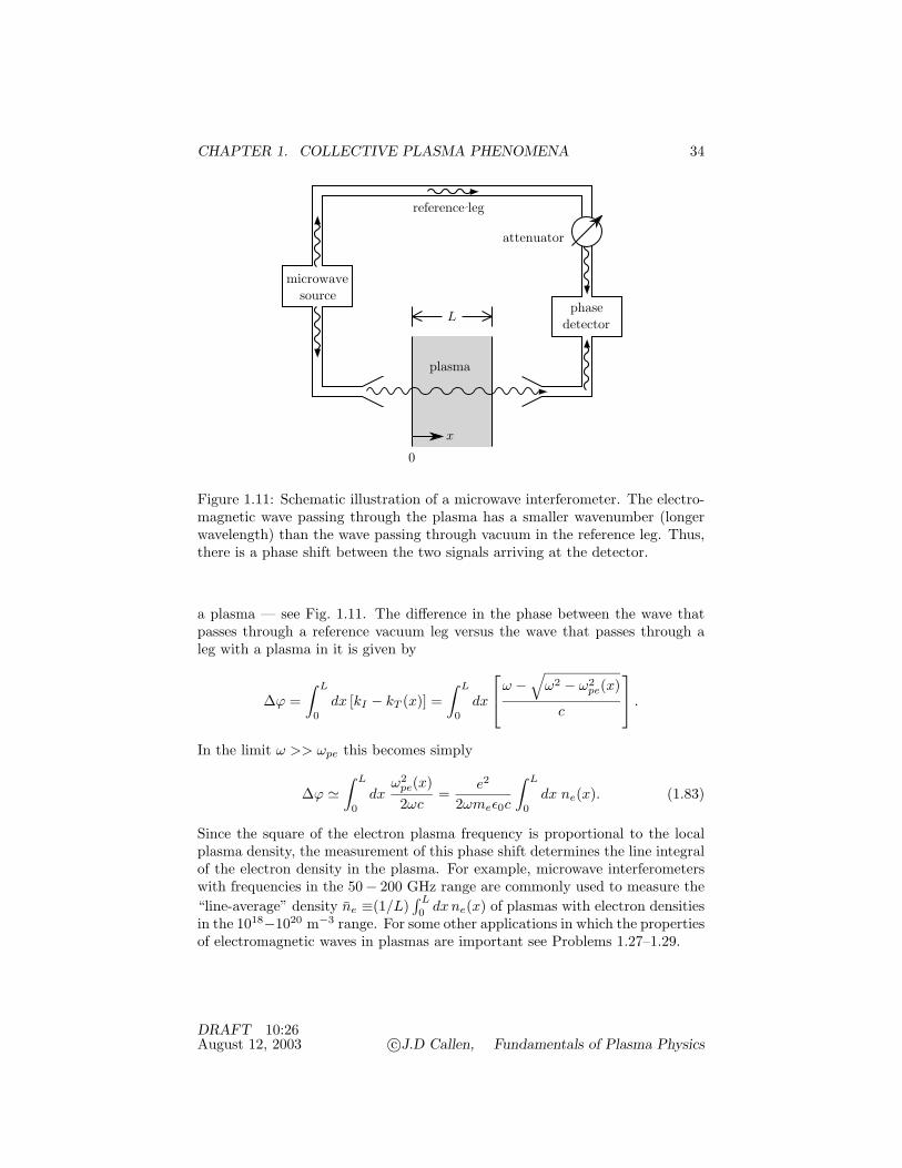
CHAPTER 1. COLLECTIVE PLASMA PHENOMENA 34
microwavesource
phasedetector
plasma
reference!leg
attenuator
L
x
0
Figure 1.11: Schematic illustration of a microwave interferometer. The electro-magnetic wave passing through the plasma has a smaller wavenumber (longerwavelength) than the wave passing through vacuum in the reference leg. Thus,there is a phase shift between the two signals arriving at the detector.
a plasma — see Fig. 1.11. The difference in the phase between the wave thatpasses through a reference vacuum leg versus the wave that passes through aleg with a plasma in it is given by
∆ϕ =∫ L
0dx [kI − kT (x)] =
∫ L
0dx
ω −√ω2 − ω2
pe(x)
c
.
In the limit ω >> ωpe this becomes simply
∆ϕ $∫ L
0dx
ω2pe(x)2ωc
=e2
2ωmeε0c
∫ L
0dx ne(x). (1.83)
Since the square of the electron plasma frequency is proportional to the localplasma density, the measurement of this phase shift determines the line integralof the electron density in the plasma. For example, microwave interferometerswith frequencies in the 50− 200 GHz range are commonly used to measure the“line-average” density ne ≡(1/L)
∫ L0 dx ne(x) of plasmas with electron densities
in the 1018−1020 m−3 range. For some other applications in which the propertiesof electromagnetic waves in plasmas are important see Problems 1.27–1.29.
DRAFT 10:26August 12, 2003 c©J.D Callen, Fundamentals of Plasma Physics

CHAPTER 1. COLLECTIVE PLASMA PHENOMENA 35
1.8 Plasma Definition and Responses
Now that we have elucidated the basic length (Debye length λD) and time(plasma period 1/ωpe) scales for collective phenomena in plasmas, we can specifyquantitatively the criteria that must be satisfied for matter to exist in the plasmastate. As we discussed in the introduction to this chapter, a general criterion forthe existence of a plasma is that charged particle interactions be predominantlycollective rather than binary in the medium. For this general criterion to besatisfied, we must require that it be satisfied in charged-particle interactions, aswell on the relevant length and time scales for collective phenomena:
1. nλ3D >> 1. The number of charged particles within a Debye cube (or
sphere) must be large so that: a) collective interactions dominate overbinary interactions at the mean interparticle separation distance; b) theenergy density embodied in the polarization electric field around a givencharged particle is small compared to a typical particle’s kinetic energy;and c) the thermal noise level is small — see (1.11), (1.14) and (1.15),respectively.
2. L >> λD. The spatial extent of a collection of charged particles mustbe large compared to the collective interaction scale length for plasmas,the Debye length λD, so that: a) the collective interactions are dominatedby bulk plasma rather than boundary effects; and b) inertial effects aredetermined locally — see (1.27) and Fig. 1.3, and (1.49), respectively.
3. ωpe >> νen. The collective inertial response frequency in a plasma, theelectron plasma frequency ωpe, must be large compared to the electron-neutral collision frequency νen, so that the fundamental inertial responses,the electrostatic electron plasma oscillations in (1.45) and the plasma os-cillation effects on electromagnetic waves in (1.75), are not damped bydissipative neutral particle collision effects.
While we have derived the basic collective phenomena in an unmagnetizedplasma, the same physical phenomena occur in magnetized plasmas (primar-ily along the magnetic field direction); hence these criteria for the existence ofthe plasma state apply to magnetized plasmas as well.
Among the three criteria for existence of the plasma state, the first one,the requirement that there are many charged particles in a Debye cube, is thenecessary condition and the most critical. After this fundamental criterion issatisfied, the second and third criteria are just checks (sufficient conditions)that the behavior of the medium will be dominated by collective plasma phe-nomena on the basic plasma length and time scales. The fundamental plasmaparameter, the number of charged particles in a Debye cube, depends on theplasma temperature and charged-particle density, i.e., nλ3
D ∝ T 3/2/n1/2. Thus,as shown in Fig. 1.12, we can exhibit the various types of plasmas that occur innature by showing where they lie relative to lines of constant nλ3
D in a plot ofelectron temperature versus electron plasma density. As shown in this figure,
DRAFT 10:26August 12, 2003 c©J.D Callen, Fundamentals of Plasma Physics

CHAPTER 1. COLLECTIVE PLASMA PHENOMENA 36
Electron!Density!(m-3)
Plasma!Frequency!fpe!(Hz)
100 105 1010 1015 1020 1025 1030 103510-2
1
102
104
106102 104 106 108 1010 1012 1014 1016 1018
Tem
pera
ture!(
eV)
inte
rste
llar
glow
disc
harg
es
flam
es
eart
h’s
mag
neto
-sp
here
inte
rpla
neta
ry
iono
-sp
here
alka
li!m
etal
plas
mas
mag
neti
c!co
nfin
emen
tex
peri
men
tsm
agne
tic
fusi
on
partially
ionized
10-11!m
1010
=!104!m
105
100
sola
r!at
mos
pher
eM
HD
gene
rato
rs
sola
rco
rona
101!m 10-2!m 10-5!m 10-8!m
iner
tial
conf
inem
ent
expe
rim
ents
iner
tial
fusi
on
Figure 1.12: Ranges of electron temperature and density for various types of lab-oratory and extraterrestial plasmas. Also shown are the characteristic plasmaparameters: electron Debye length λDe (constant along the dashed lines), num-ber of charged particles in a Debye cube neλ3
De (constant along solid lines), andelectron plasma frequency ωpe (constant along vertical lines). Also indicated isthe electron temperature range below which the medium is not fully ionized,which is determined from the Saha equation [see Section A.7 and in particular(??) and (??)].
DRAFT 10:26August 12, 2003 c©J.D Callen, Fundamentals of Plasma Physics

CHAPTER 1. COLLECTIVE PLASMA PHENOMENA 37
the plasma state spans an enormous parameter range — 26 orders of magnitudein density and 7 orders of magnitude in temperature!
Almost all plasmas are electrically quasineutral (i.e., ρq =∑
s nsqs $ 0) onlength scales longer than the Debye length λD. (Notable exceptions are theelectron-rich, non-neutral magnetized plasmas — see references listed below.)On length scales shorter than a Debye length the local charge density and po-tentials are dominated by the effects of the discrete charged particles. However,on length scales longer than the Debye length the collective, plasma polariza-tion effects dominate and the plasma is quasineutral. The use of a quasineutralapproximation for scale lengths longer than a Debye length is often called the“plasma approximation.”
Slow processes (ω << vT /δx ∼ kvT ) in a plasma are governed by the adia-batic response, as discussed in Section 1.1. Fast processes (ω >> vT /δx ∼ kvT )are governed by the inertial response, as discussed in Section 1.4. Becausethe electron thermal speed is usually much greater than the ion thermal speed(vTe ∼ √mi/me vTi ∼ 43 vTi >> vTi for Te ∼ Ti), the electrons and ions ina plasma can respond differently to perturbations — for kvTi << ω << kvTe
electrons respond adiabatically while the ions respond inertially, as discussed inSection 1.4.
The response of the plasma to electric field perturbations leads to polariza-tion of the plasma, and hence to a dielectric response for the plasma medium.The plasma responses in the various frequency regimes can be summarized interms of the density and dielectric responses to small (i.e., linearizable) wavelikeperturbations of the form exp (ik · x− iωt) in an infinite, homogeneous electron-ion plasma as follows:
Adiabatic (A) electrons and ions: ω / kvTi, kvTe; Debye shielding;
nA $ − qφ
Tn0; εA (k,ω) $ ε0
[1 +
1k2
(1λ2
De
+1λ2
Di
)]. (1.84)
Adiabatic electrons, inertial ions: kvTi / ω / kvTe; ion acoustic waves;
neA $ eφ
Ten0e,
ZieniI
ε0$ − ω2
pi
ω2∇· E; εS(k,ω) $ ε0
[1 +
1k2λ2
De
− ω2pi
ω2
].
(1.85)
Inertial (I) electrons and ions: kvTi, kvTe / ω; plasma oscillations;
qsnsI
ε0$ − ω2
ps
ω2∇· E; εI(k,ω) $
[1 − ω2
pe
ω2− ω2
pi
ω2
]. (1.86)
As can be seen from these various responses, a plasma is an electrically ac-tive medium with a frequency- and wavenumber-dependent polarizability anddielectric response function. As discussed before, these responses are only ap-plicable for spatially and temporally varying perturbations — they all divergefor ω,k → 0.
DRAFT 10:26August 12, 2003 c©J.D Callen, Fundamentals of Plasma Physics

CHAPTER 1. COLLECTIVE PLASMA PHENOMENA 38
Within the approximations employed in this chapter, all the basic phenom-ena in plasmas that we have discussed are reactive with no dissipation. Dissi-pation would be caused by polarization components that are 90 out of phasewith the electric field perturbations, which for exp (ik · x − iωt) perturbationswould be indicated by an imaginary part of the dielectric ε.
Implicitly, we have been considering the plasma to be “collisionless.” Pre-suming collisions with neutrals are negligible (ωp >> νn), there are two typesof effects that lead to evanescence of waves in a plasma — Coulomb collisions,which will be discussed in Chapter 2, and wave-particle resonance effects (Lan-dau damping), which will be discussed in Chapter 8. Since the thermal noisefluctuation energy induced by two-particle correlations (or Coulomb collisions)in a plasma is only a small fraction 1/
(nλ3
D
)<< 1 of the thermal energy in
a plasma, we can anticipate that the average Coulomb collision frequency willalso be small: ν ∼ ωp/
(nλ3
D
)<< ωp. Cumulative small-angle Coulomb colli-
sions enhance the Coulomb collision rate ν by a factor of order ln(nλ3
D
)— see
Chapter 2 — but do not change the basic conclusion that the Coulomb collisionrate is slow in a plasma as long as nλ3
D >> 1. The wave-particle resonanceeffects will be largest when ω ∼ kvT , i.e., when the wave phase speed ω/k isof order the most probable thermal speed vT ≡ √2T/m of one of the speciesof charged particles in a plasma. Thus, wave-particle resonance effects will leadto evanescence of waves (Landau damping) for ω/k ∼ vTi or vTe. These wavephase speeds and corresponding frequencies are between the frequency rangeswe have considered in this chapter and require a kinetic plasma description.Wave-particle resonance effects and Landau damping are discussed in Chapter8, and in particular in Section 8.2.
REFERENCES AND SUGGESTED READING
Discussions of plasma sheath and Langmuir probe theory can be found in
D. Bohm in Characteristics of Electrical Discharges in Magnetic Fields, A.Guthrie and R.K. Wakerling, eds. (1949) [?].
F.F. Chen, “Electrical Probes,” in Plasma Diagnostic Techniques, R.H. Huddle-stone and S.L. Leonard, eds. (1965), Chapt. 4 [?].
L. Schott and R.L.F. Boyd in Plasma Diagnostics, W. Lochte-Holtgreven, ed.(1968) [?].
J.D. Swift and M.J.R. Schwar, Electric Probes for Plasma Diagnostics (1971)[?].
P.M. Chung, L. Talbot and K.J. Touryan, Electric Probes in Stationary andFlowing Plasmas (1975) [?].
P.C. Stangeby, “The Plasma Sheath,” in Physics of Plasma-Wall Interactionsin Controlled Fusion, D.E. Post and R. Behrisch, eds. (1985), Vol. 131, p. 41[?].
Hutchinson, Principles of Plasma Diagnostics (1987), Chapt. 3 [?].
N. Hershkowitz, “How Langmuir Probes Work,” in Plasma Diagnostics, O. Au-ciello and D.L. Flamm, eds., (1990) [?].
DRAFT 10:26August 12, 2003 c©J.D Callen, Fundamentals of Plasma Physics
CHAPTER 1. COLLECTIVE PLASMA PHENOMENA 39
Recent books that discuss the various types of plasmas indicated in Fig. 1.12,some of which are beyond the scope of this book, include
Magnetically confined plasmas for controlled fusion:
Rose and Clark, Jr., Plasmas and Controlled Fusion (1961) [?].
Miyamoto, Plasma Physics for Nuclear Fusion (1980) [?].
Miyamoto, Fundamentals of Plasma Physics and Controlled Fusion (1997) [?].
Stacey, Fusion Plasma Analysis (1981) [?].
Teller, ed., Fusion (1981), Vol. I, Parts A & B [?].
Nishikawa and Wakatani, Plasma Physics, Basic Theory with Fusion Applica-tions (1990) [?].
Hazeltine and Meiss, Plasma Confinement (1992) [?].
White, Theory of Tokamak Plasmas (1989) [?].
Goldston and Rutherford, Introduction to Plasma Physics (1995) [?].
Laser-produced plasmas for inertial confinement fusion:
Kruer, The Physics of Laser Plasma Interactions (1988) [?].
Lindl, Inertial Confinement Fusion (1995) [?].
Space plasmas:
Parks, Physics of Space Plasmas, An Introduction (1991) [?].
Gombosi, Physics of the Space Environment (1998) [?].
Cosmic plasmas:
Alfven and Falthammer, Cosmical Electrodynamics, Fundamental Principles(1963) [?].
Parker, Cosmical Magnetic Fields, Their Origin And Their Activity (1979) [?].
Sturrock, Plasma Physics, An introduction to the theory of astrophysical, geo-physical, and laboratory plasmas (1994) [?].
Choudhuri, The Physics of Fluids and Plasmas, An Introduction for Astrophysi-cists (1998) [?].
Partially ionized plasmas and plasma processing:
Chapman, Glow Discharge Processes (1980) [?].
Lieberman and Lichtenberg, Principles of Plasma Discharges and Materials Pro-cessing (1994) [?].
Nonneutral plasmas:
Davidson, Physics of Nonneutral Plasmas (1990) [?].
Marshall, Free Electron Lasers (1985) [?].
DRAFT 10:26August 12, 2003 c©J.D Callen, Fundamentals of Plasma Physics

CHAPTER 1. COLLECTIVE PLASMA PHENOMENA 40
PROBLEMS
1.1 Evaluate the scale lengths bclmin, n−1/3
e and λDe for an electron-proton plasmain a typical small-scale magnetic confinement experiment (e.g., a university-based tokamak) with ne = 2 × 10¹⁹ m−3, Te = Ti = 300 eV. Compare themto the Bohr radius, de Broglie wavelength, and the classical electron radiusre = e2/(4πε0mec
2). Discuss the physical significance of each of these scalelengths. Over what length scale will collective effects occur in such a plasma? /
1.2 Calculate the plasma parameter nλ3D for the plasma described in the preceding
problem. Estimate the effective temperature for thermal noise in such a plasma.Compare this thermal noise temperature to normal room temperature. /
1.3 Consider a hypothetical situation in which all the electrons in a homogeneousand quasineutral but bounded plasma are displaced a small distance x in the ex
direction. Show that in the bulk of the plasma the electric field is unchanged,but that in a layer of width x at the plasma edge there is an electric field.How large a displacement x induces a maximum potential change equal to theelectron temperature in the plasma? Compare this length to the electron Debyelength λDe and discuss why such a comparison is relevant. //
1.4 Determine the one-dimensional potential distribution in a plasma around aninfinite sheet charge with a one-dimensional surface “test” charge density givenby ρq = σtδ(x − xt). ///
1.5 Show that for a two-dimensional situation of an appropriately modified form of(1.7) the potential around a line charge in a plasma is given by
φt(x) = (2λt/4πε0)K0(|x − xt|/λD)
in which λt is the line charge density (coulombs/m) for a line charge of infinitelength placed at x = xt and K0 is the modified Bessel function of the secondkind of order zero. ///
1.6 Show that the potential given by (1.10) is the Green function for the adiabatic(Debye shielding) response to a free charge density ρfree(x) in an infinite, homo-geneous plasma, and thus that the general potential solution is given by
φ(x) =
∫d3x′ ρfree(x
′) exp(−|x − x′|/λD)4πε0 |x − x′| .
Discuss the physical scale lengths over which this Green’s function solution isvalid. Compare this result to the corresponding potential induced by a chargedensity in vacuum given in (??). ///
1.7 Show that the combination of the charge of a test particle and the polarizationcharge density it induces produces a vanishing net charge Q in the plasma. //
1.8 A spherical spacecraft orbiting the earth in a geostationary orbit finds itselfimmersed in a plasma that typically has an electron density of about 106 m−3
and temperature of about 100 eV. Sketch the spatial variation of the electricpotential around the spacecraft, indicating the magnitudes of the potential andspatial scale lengths involved. To what potential does the spacecraft charge uprelative to its surroundings? /
DRAFT 10:26August 12, 2003 c©J.D Callen, Fundamentals of Plasma Physics

CHAPTER 1. COLLECTIVE PLASMA PHENOMENA 41
1.9 A spherical probe 3 mm in diameter is inserted into a fully ionized electron-proton plasma generated by microwave heating power applied to a hydrogen gasand has ne = 1015 m−3, Te = 10 eV, Ti = 1 eV. What is the Debye length insuch a plasma? Is it large or small compared to the probe size? If the probe isbiased to −10 V, how much current would it draw? /*
1.10 It is proposed to put a wire screen into the plasma described in the precedingproblem and bias it so as to exclude plasma from the region behind the screen.Taking account of sheath effects, how closely spaced must the screen wires beso as to block a substantial fraction of the plasma? To what potential shouldthe probe be biased? /*
1.11 The electron temperature in low energy density plasmas can be measured with a“double probe” — a single assembly with two identical but differentially biasedLangmuir probes that electrically floats and draws no net current from theplasma. Show that the current flowing between the two probes is given by
I = 2 ISi tanh (e∆Φ/2Te)
in which ∆Φ is the potential difference (voltage) between the two probes. //*
1.12 The “static” electrical admittance Y (inverse of impedance Z) of a sheath isgiven by ∂I/∂ΦB . At what bias potential ΦB should this partial derivativebe evaluated? Show that the sheath admittance is given approximately byY # I/(Te/e). Up to what frequency will this estimate be valid? //*
1.13 For large negative “wall” potentials (|ΦW | >> Te/e) applied between two gridsin a planar diode the electrical current is limited by space charge effects. De-rive the Child-Langmuir law for this limiting current for a grid separation d asfollows. First, using (1.27) show that when the sheath thickness xS → d andΦ∞ → ΦW , the ion speed V∞ that corresponds to the space-charge-limited ionflow at the sheath edge can be written in terms of the wall potential ΦW andthe grid separation d. Then, show that the (ion) current density into the sheathregion between the grids is given by
J =49
√2emi
ε0|ΦW |3/2
d2= (neeVW )
(49
)(λ2
DΦ
d2
)in which VW ≡ (2e|ΦW |/mi)
1/2 is the ion speed at the wall, and λDΦ =(ε0|ΦW |/nee)
1/2 is an effective Debye length. //*
1.14 In the Plasma Source Ion Implantation (PSII) technique [J.R. Conrad, J.L.Radtke, R.A. Dodd, F.J. Worzola, N.C. Tran, J. Appl. Phys. 62, 4591 (1987)],the target to be bombarded is inserted into a plasma with parameters ne ∼109cm−3 and Te ∼ 2 eV, and a natural sheath is allowed to form around it.Then, the target is rapidly biased to a very large (≥ 30 kV) negative potentialΦB . This expels the lighter electrons from the region around the object, whichin turn causes an “ion matrix” to be formed there. On what time scales arethe electrons expelled, and the new sheath formed? What is the approximatemaximum energy and current density of the ions bombarding the target beforethe new sheath forms? Compare this current density to that given by the Child-Langmuir law discussed in the preceding problem. Finally, estimate the fluence(ions/cm2) per pulse and the number of pulses required to inject an atomicmonolayer of ions in the target. ///*
DRAFT 10:26August 12, 2003 c©J.D Callen, Fundamentals of Plasma Physics

CHAPTER 1. COLLECTIVE PLASMA PHENOMENA 42
1.15 Consider an impure laboratory plasma composed of a number of different typesof ions: protons with np = 3 ×10¹⁹ m−3, fully ionized carbon ions with 10% ofthe proton density and iron ions that are 23 times ionized (Lithium-like chargestates) with 1% of the proton density. What is the electron density and theoverall plasma frequency in this plasma? Also, what is the dielectric “constant”for 90 GHz electrostatic fluctuations in this plasma? /
1.16 Consider electrostatic plasma oscillations in an electron-positron plasma, suchas could occur in interstellar space, with ne− = ne+ = 106 m−3. What is theplasma frequency for such oscillations? Assume the electrons and positrons havetemperatures of 100 eV and that the cross-section for an annihilation interactionbetween them is given by π times the square of the classical electron radiusre = e2/(4πε0mec
2), i.e., σan ∼ π r2e . What is their annihilation reaction
rate? Compare this annihilation rate to the plasma frequency. /
1.17 Consider a situation where an oscillating potential is applied across two plateson either side of a plasma such as that described in Problem 1.9. Assume theplates are separated by 10 cm and that the potential oscillates at 100 kHz.What is the dielectric “constant” for these oscillations? What is the ratio ofthe energy density in the plasma polarization fluctuations to that in the electricfield fluctuations? /
1.18 Calculate the weak dissipation induced by Coulomb collisions (ν << ωpe) of ω ∼ωpe electrostatic oscillations in a plasma as follows. Add a collisional dynamicalfriction force − ν mev [cf., (??)] to (1.31) and show that for E = E sinωt theperturbed velocity of electrons is then given for t >> 1/ν by
v # eEωme
[cosωt − (ν/ω) sinωt].
Next, calculate the average of the Joule heating in the plasma by the oscillationsover an oscillation period 2π/ω, i.e., 〈J · E〉ωt. Finally, use a wave energy balanceequation [cf., (??)] to show that
1〈wE〉ωt
∂〈wE〉ωt
∂t= − 〈J · E〉ωt
〈wE〉ωt# − 2ν
1 + ω2/ω2pe
in which 〈wE〉ωt is the average of the electrostatic wave energy density in theplasma over an oscillation period. ///
1.19 Consider a hypothetical situation in which all the electrons in a thin slab aredisplaced a small distance x0 in the ex direction. Show that the electric fieldinduced by this displacement is given by E = (n0e/ε0) x ex in the region wherethe electrons are displaced. Then, show from Newton’s second law that thisforce causes the position of the slab of displaced electrons to oscillate at theelectron plasma frequency. //
1.20 Taking account of plasma sheath effects, sketch the spatial variation of thepotential Φ(x) between the plates of a capacitor filled with plasma assumingthe capacitor has a potential Φ ∼ 3 Te/e applied across it. Next, consider acase where an oscillating potential Φ = Φ0 sinωt is applied across the plasmacapacitor with Φ0 = 10 Te/e and ω = ωpe/10. If the capacitor plate separationis L (>> λD), how large is the electric field component oscillating at frequencyω in the body of the plasma? //
DRAFT 10:26August 12, 2003 c©J.D Callen, Fundamentals of Plasma Physics

CHAPTER 1. COLLECTIVE PLASMA PHENOMENA 43
1.21 Show that for a one-dimensional wave perturbation in a plasma with E(x, t) =E ex sin(kx−ωt) the nonlinear terms in (1.31) are negligible in (1.32) when thewave-induced velocity “jitter” in the particle motion, vjitter ≡ qE/mω, is smallcompared to the wave phase speed ω/k, or alternatively when kxjitter << 1. //
1.22 Consider the propagation of ion acoustic waves in a typical hollow cathode arcdischarge composed of electrons and doubly charged Argon ions with ne = 1019
m−3, Te = 10 eV, Ti = 1 eV. Discuss why the conditions for propagation ofion acoustic waves are satisfied in this plasma. What is the ion acoustic speedin this plasma? Compare it to the speed of sound in air at the earth’s surface.With what wavelength and phase speed will externally imposed waves with afrequency of 100 MHz propagate in this plasma? /
1.23 Show that the transverse electric field Et induced by a small free current Jfree
in a plasma is governed by the equation(∇2 − ω2
pe
c2
)Et − 1
c2
∂2Et
∂t2= µ0
∂Jfree
∂t.
Then, show that a Green’s function solution of this equation in an infinite,homogeneous plasma which satisfies this equation is
Et = −µ0
4π
∫d3x′
[∂Jfree(x
′, t′)/∂t′
|x − x′| exp
(− |x − x′|
c/ωpe
)]ret
in which the square bracket [ ]ret means that the time t′ is to be evaluated atthe retarded time t′ = t − |x − x′|/c. ///
1.24 Use the solution in the preceding problem to calculate the transverse electricfield Et caused by the current qtvδ[x − x(t)] produced by a nonrelativistic testparticle moving along the trajectory x = x(t) in a plasma. Show that thistransverse electric field points in the direction of test particle motion. Also,show that for |x − x(t)| < λD its magnitude is of order v2/c2 << 1 comparedto the longitudinal electric field produced by the electrostatic potential φt in(1.10). ///
1.25 Plot the wave dispersion diagrams for electrostatic ion acoustic waves and elec-tromagnetic plasma waves (i.e., Figs. 1.8 and 1.9) in the plasma described inProblem 1.22 on a single ω versus k diagram with approximately linear scales.Indicate in which regions of this diagram adiabatic and inertial responses forthe electrons and ions are applicable. /
1.26 A 140 GHz microwave interferometer set up across a 30 cm thick column ofplasma measures a phase shift of 240. What is the “line-average” plasmadensity in the column? /
1.27 Amateur radio operators routinely communicate via shortwave radio over longdistances around the earth. Since communication by direct line of sight is notpossible because of the curvature of the earth’s surface, the waves must be re-flected from the ionosphere above the earth’s surface. What frequency rangecorresponds to the 10 to 40 meter free space wavelength range used by ama-teur radio operators for these communications? What is the minimum electrondensity and height of the ionosphere above the earth’s surface for single-bouncecommunications over the approximately 6000 km from the United States toWestern Europe? /
DRAFT 10:26August 12, 2003 c©J.D Callen, Fundamentals of Plasma Physics

CHAPTER 1. COLLECTIVE PLASMA PHENOMENA 44
1.28 During reentry of satellites into the earth’s upper atmosphere, microwave com-munications in the 300 MHz frequency range are “blacked out” by the plasmaformed in the heated air around the satellite. How high must the plasma den-sity be around the satellite and how thick must the plasma be to cause thecommunications blackout? /
1.29 In one type of inertial fusion experiment, intense light from a laser is shined ona frozen hydrogen pellet. As the laser light is absorbed it heats up the pelletand produces a plasma on its surface. Light from a Neodynium glass laser (λ =1.06 µm) is ultimately observed to be reflected from the pellet. How high mustthe density of “free” electrons be in the plasma around the pellet? Comparethis density to the original solid density of the pellet. How thick must the layerof free electrons be to reflect (or refract) the light waves? Compare this lengthto a typical pellet radius of 3 mm. /
1.30 In plasma processing of materials for the semiconductor industry an inert, lowpressure gas is partially ionized by radiofrequency waves in a vacuum chamber.Consider a case where the initial gas is Argon at a pressure of 10−4 mm Hg (a760 mm column of mercury corresponds to atmospheric pressure), the electrondensity is 107 cm−3, the electron temperature is 3 eV and the temperature of thesingly charged Argon ions is 0.1 eV. What is the degree of ionization in this gas?Estimate the electron-neutral collision frequency νen using an electron-neutralcross-section of 103πa2
0 where a0 is the Bohr radius. Does this medium satisfyall the criteria for being a plasma? How large must it be to satisfy the lengthcriterion? /
1.31 An oscillating potential of 3 volts at a frequency of 1 MHz is applied to a probeinserted into the plasma described in Problem 1.9. Over what distance rangesfrom the probe can adiabatic or inertial responses be used for the electrons andfor the ions in this plasma? /
1.32 What is the dielectric “constant” for externally imposed waves with a frequencyof 1 MHz and a wavelength of 5 cm in the plasma described in problem 1.9?What would the dielectric “constant” be if the wavelength was increased to 500cm? /
DRAFT 10:26August 12, 2003 c©J.D Callen, Fundamentals of Plasma Physics
CHAPTER 2. COULOMB COLLISIONS 1
Chapter 2
Coulomb Collisions
The characteristics and effects of Coulomb collisions between charged particlesin a plasma are very different from those of the more commonly understoodcollisions of neutral particles. The fundamental differences can be illustrated byexamining trajectories of neutral and charged particles as they move through apartially ionized gas. As shown in Fig. 2.1, neutral particles move independentlyalong straight-line trajectories between distinct collision events. Collisions occurwhen neutral atoms or molecules come within an atomic radius (of order 1 A=10−10 m — see Section A.7) of another particle (a neutral or a charged particle)and the electric field force associated with the atomic potential (of order eV) isoperative; the resultant “strong,” typically inelastic, collision causes the initialneutral to be scattered in an approximately random direction.
In contrast, as a charged “test” particle moves through an ionized gas it si-multaneously experiences the weak Coulomb electric field forces surrounding allthe nearby charged particles, and its direction of motion is deflected as it passesby each of them, with the closest encounters producing the largest deflections— see Fig. 2.2. As was discussed in Section 1.2, the Coulomb potential aroundany particular background charged particle in a plasma is collectively shieldedout at distances beyond a Debye length. Thus, the only background particlesthat exert a significant force on the test particle’s motion are those within abouta Debye length. However, because plasmas usually have a very large numberof particles within a Debye sphere [(4π/3)nλ3
D >> 1], even in traversing onlya Debye length the test particle’s motion is influenced by a very large numberof background particles. The Coulomb electric field forces produced by indi-vidual background particles are small and can be assumed to be experiencedrandomly by the test particle as it passes close to individual background parti-cles — as indicated in the electron trajectory shown in Fig. 2.2. The effect ofmany successive, elastic Coulomb “collisions” of a test particle with backgroundcharged particles leads to a random walk (Brownian motion) process. Thus,the effects of the many cumulative small-angle, elastic Coulomb collisions arediffusion of the test particle’s direction of motion (at constant energy in thecenter-of-momentum frame) and consequently deceleration of the test particle’s
DRAFT 14:53August 25, 2003 c©J.D Callen, Fundamentals of Plasma Physics

CHAPTER 2. COULOMB COLLISIONS 2
+
+
+ ++
++
+
+
+
+
++
+
+ +
+
+
+
+
+
+
+
+
++
+
+
+
+
++ +
+
+
+
+
++
+
+
+
+ +
+
++
+
+
+
+
+
+
+
+
+
+
++
-
-
-
-
-
-
-
-
-
-
--
-
-
- --
-
-
-
-
-
-
-
-
-- --
- -
-
-
-
---
--
-
--
-
-
-
-
-
-
-
-
-
-
-
-
-
-
-
-
-oooo o
oo
o
o
o
o
o
o
o
o
o
o
o
o
Figure 2.1: The trajectory of a neutral particle in a partially ionized gas exhibits“straight-line” motion between abrupt atomic collisions. In this and the nextfigure, the (assumed stationary) random positions of “background” particles inthe partially ionized plasma that the incident “test” particle could interact withare indicated as follows: neutral particles (circles), electrons (minus signs) andions (plus signs).
+
+
+ ++
++
+
+
+
+
++
+
+ +
+
+
+
+
+
+
+
+
++
+
+
+
+
++ +
+
+
+
+
++
+
+
+
+ +
+
++
+
+
+
+
+
+
+
+
+
+
++
-
-
-
-
-
-
-
-
-
-
--
-
-
- --
-
-
-
-
-
-
-
-
-- --
- -
-
-
-
---
--
-
--
-
-
-
-
-
-
-
-
-
-
-
-
-
-
-
-
-o
ooo o
oo
o
o
o
o
o
o
o
o
o
o
o
_
Figure 2.2: The trajectory of a “test” charged particle (electron) in a partiallyionized gas exhibits continuous small-angle deflections or scatterings of its di-rection of motion. The largest deflections occur when a charged particle passesclose to another charged particle.
DRAFT 14:53August 25, 2003 c©J.D Callen, Fundamentals of Plasma Physics
CHAPTER 2. COULOMB COLLISIONS 3
initial, directed velocity. Exploration of these Coulomb collision effects is themain subject of this chapter.
Because electrons have less inertia and typically have larger speeds thanions, their collision rates are usually the largest in plasmas. Thus, we first con-sider the momentum loss and velocity-space diffusion of a test electron as itmoves through a plasma. Electron collisions are investigated using the Lorentz(simplest) collision model in which their collisions are assumed to occur onlywith a background of stationary ions. Next, since the collisional effects de-crease with electron speed, we determine the energy (usually on the high energytail of a Maxwellian distribution) at which electrons “run away” in response toan electric field; also, the plasma electrical resistivity is determined by balanc-ing, for the backgound electron distribution, the average collisional decelerationagainst the electron acceleration induced by an electric field. Then, we discussphenomenologically the various Coulomb collisional processes (momentum loss,energy exchange and their time scales) that occur between electrons and ions ina plasma. The chapter concludes with sections that develop a more completemodel of Coulomb collision effects that takes into account collisions with alltypes of background charged particles that are also in motion. Finally, applica-tions of this more complete model to the thermalization of a fast ion in a plasmaand to the evolution of the velocity of any type of test particle are discussed.
2.1 Lorentz Collision Model
To illustrate Coulomb collision effects, we first consider the momentum loss andvelocity diffusion of a test electron moving through a randomly distributed back-ground of plasma ions that have charge Zie and are stationary. (The particlesin the background that are being collided with are sometimes called field par-ticles.) The background plasma electrons, which must be present for quasineu-trality, will be neglected except insofar as they provide Debye shielding of theCoulomb potentials around the background ions. However, the “test” electroncan be thought of as being just one particular electron in the plasma. Thissimplest and most fundamental model of collisional processes in a plasma iscalled the Lorentz collision model . It provides a reasonably accurate descrip-tion of electron-ion collisional processes and, in the limit Zi >> 1 (see Section2.8) where electron-electron collisional effects become negligible, for electronCoulomb collision processes as a whole.
The electron test particle velocity v will be assumed to be large compared tothe change ∆v due to any individual Coulomb interaction with an ion. Hence,the test electron will be only slightly deflected from its straight-line trajectoryduring a single collision. Figure 2.3 shows a convenient geometry for describingthe Coulomb collision process.1 In the rest frame of the electron, the backgroundion, which we place at the origin of the coordinate system, is seen to be moving
1The geometry shown in Fig. 2.3 and the pedagogical approach we use for exploringCoulomb collision processes follows that developed in Chapter 13 of Jackson, Classical Elec-trodynamics, 1st and 2nd Editions (1962, 1975).
DRAFT 14:53August 25, 2003 c©J.D Callen, Fundamentals of Plasma Physics

CHAPTER 2. COULOMB COLLISIONS 4
electron
ion
b!cos!φ
b!sin!φ
b
y
z
x
vt
φ
v
Figure 2.3: Geometry for considering the Coulomb collision of an electron havingcharge qe = −e with an ion of charge qi = Zie. The ion is placed at the originof the coordinate system, which in the electron rest frame is moving in the −ez
direction at the electron speed v. The electron passes the ion at a distance b atthe closest point, which occurs at t = 0.
with a velocity −v ez along a straight-line trajectory x(t) = −vt ez. The electronis instantaneously at the position
x = b (ex cosϕ + ey sinϕ) + vt ez, |x| =(b2 + v2t2
)1/2, (2.1)
in which b is known as the impact parameter . It is the distance of closestapproach, which by assumption will occur at time t = 0. The electrostaticpotential around the ion is the Coulomb potential φ(x) = Zie/(4πε0|x|).Thus, the electric field force experienced by the test electron with charge qe = −eat its position x is
F = qeE = − (−e)∇(
Zie
4πε0|x|)
= − Zie2x4πε0|x|3 . (2.2)
Next, we calculate the momentum impulse me∆v on the test electron as itpasses the background ion. Integrating Newton’s second law (m dv/dt = F)over time from long before (t → −∞) to long after (t → +∞) the Coulomb“collision” that takes place during the time t where |t| ∼ ∆t ∼ b/v, we see thata single electron-ion Coulomb collision induces:
me∆v =∫ ∞
−∞dt qeE = −
∫ ∞
−∞dt
Zie2x4πε0|x|3 . (2.3)
DRAFT 14:53August 25, 2003 c©J.D Callen, Fundamentals of Plasma Physics

CHAPTER 2. COULOMB COLLISIONS 5
Using the specification of x in (2.1), we find
∆v⊥ = − Zie2b
4πε0me(ex cosϕ + ey sinϕ)
∫ ∞
−∞
dt
(b2 + v2t2)3/2
= − 2Zie2
4πε0mebv(ex cosϕ + ey sinϕ) . (2.4)
(This expression is relativistically correct if me is replaced by the relativisticmass γ me = me/
√1 − v2/c2.) Note that the perturbation of the electron ve-
locity is in a direction perpendicular to its direction of motion. There is nocomponent along the direction of particle motion (ez direction), at least in thisfirst order where the particle trajectory is the unperturbed one — because the zcomponent of the Coulomb force is an odd function of z or t. Hence, to this firstor lowest order there is no momentum loss by the particle. Rather, a typicalelectron is only deflected by a small angle ∆ϑ ∼ ∆v⊥/v << 1 in velocity space.Using a typical impact parameter b ∼ n−1/3
e , the average inter-particle spacingin the plasma, and a typical electron speed v ∼ vTe, the typical deflection angleis ∆ϑ ∼ 1/[4π(neλ3
D)2/3] << 1.Since the background ion is at rest in the Lorentz collision model, the electron
energy is conserved during the elastic Coulomb collision process. Thus, we haveme|v|2/2 = me|v + ∆v|2/2 = m(|v|2 + 2v · ∆v + ∆v · ∆v), from which we findthat the component of ∆v parallel to v can be determined from
v · ∆v = − 12
∆v · ∆v & − 12
∆v⊥· ∆v⊥, (2.5)
as indicated in Fig. 2.4. That is, for electron energy conservation the change ofelectron velocity along its direction of motion is given by half of the negative ofthe square of the transverse deflection. The net velocity change along the ez orparallel (‖) direction of electron motion which is induced by a single Coulombcollision with a background ion is thus (v · ∆v ≡ v ∆v‖)
∆v‖ & − 12v
∆v⊥· ∆v⊥ = − 2Z2i e4
4πε02m2eb
2v3. (2.6)
Note that while ∆v⊥ is a first order quantity in terms of the weak Coulombelectric field between the two particles given in (2.2), ∆v‖ is a second orderquantity, as evidenced by the square of the 4πε0 factor in the denominator.The result in (2.6) can also be obtained directly by integrating the Coulombelectric field force along a perturbed (by the Coulomb collision) trajectory ratherthan the straight-line electron trajectory that was assumed in the precedinganalysis — see Problem 2.5.
Next, we take account of the entire background distribution of ions, assumingthat the electron collisions with individual ions are statistically random andthus that their effects can be summed independently. For a density ni of ions,adopting a cylindrical geometry in which the radius is b and the azimuthal angleis ϕ, the number of ions passed by the electron per unit time is ni
∫d3x/dt =
DRAFT 14:53August 25, 2003 c©J.D Callen, Fundamentals of Plasma Physics

CHAPTER 2. COULOMB COLLISIONS 6
constantenergysurface
v!+!∆v
v
∆v ∆v⊥
∆v‖
Figure 2.4: Change in electron velocity vector from v before the Coulomb colli-sion to v + ∆v afterward. The change takes place at constant electron energy,which means constant radius in this diagram, and hence results in ∆v‖ < 0.
ni (dz/dt)∫
dA = ni v∫
dϕ∫
b db (cf., Fig. 2.2). Hence, the net or ensembleaverage2 Coulomb collisional force in the direction of electron motion is givenby
〈F‖〉 ≡ me〈∆v‖〉
∆t= niv
∫ 2π
0dϕ
∫ ∞
0b db me∆v‖ = − 4π niZ2
i e4
4πε02mev2
∫db
b. (2.7)
Here, ∆t is a typical interaction time for individual Coloumb collisions (∆t ∼b/v ∼ 1/[ωpe(neλ3
D)1/3]), which is short compared to the time for the test elec-tron to traverse a Debye sphere (∼ λDe/v ∼ λDe/vTe ∼ 1/ωpe), and certainlyshort compared to the time scale on which the test particle velocity v changessignificantly due to Coulomb collisions [∆t << 1/ν, where ν is the collisionfrequency defined in (2.14) below].
The integral over the impact parameter b in (2.7) is divergent at both itsupper and lower limits:
∫ ∞0 d b/b =⇒ ln(∞/0) ?! We restrict its range of inte-
gration through physical considerations that can be more rigorously justified bydetailed analyses. The maximum impact parameter will be taken to be the De-bye length since the Coulomb electric field force decays exponentially in space
2In an ensemble average one averages over an infinite number of similar plasmas (“realiza-tions”) that have the same number of particles and macroscopic parameters (e.g., density n,temperature T ) but whose particle positions vary randomly from one realization to the next— see Section A.5.
DRAFT 14:53August 25, 2003 c©J.D Callen, Fundamentals of Plasma Physics
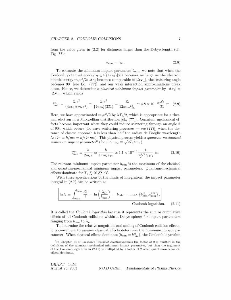
CHAPTER 2. COULOMB COLLISIONS 7
from the value given in (2.2) for distances larger than the Debye length (cf.,Fig. ??):
bmax = λD. (2.8)
To estimate the minimum impact parameter bmin, we note that when theCoulomb potential energy qeqi/(4πε0|x|) becomes as large as the electronkinetic energy mev2/2: ∆v‖ becomes comparable to |∆v⊥|, the scattering anglebecomes 90o [see Eq. (??)], and our weak interaction approximations breakdown. Hence, we determine a classical minimum impact parameter by
∣∣∆v‖∣∣ =
|∆v⊥|, which yields
bclmin =
Zie2
4πε0(mev2)& Zie2
4πε0(3Te)=
Zi
12πneλ2De
& 4.8 × 10⁻¹⁰ Zi
Tem. (2.9)
Here, we have approximated mev2/2 by 3Te/2, which is appropriate for a ther-mal electron in a Maxwellian distribution [cf., (??)]. Quantum mechanical ef-fects become important when they could induce scattering through an angle ϑof 90o, which occurs [for wave scattering processes — see (??)]) when the dis-tance of closest approach b is less than half the radian de Broglie wavelengthλh/2π ≡ h/mv = h/(2πmv). This physical process yields a quantum-mechanicalminimum impact parameter3 (for v & vTe ≡ √
2Te/me )
bqmmin ≡ h
2mev& h
4πmevTe& 1.1 × 10⁻¹⁰ 1
T 1/2e (eV)
m. (2.10)
The relevant minimum impact parameter bmin is the maximum of the classicaland quantum-mechanical minimum impact parameters. Quantum-mechanicaleffects dominate for Te
>∼ 20 Z2i eV.
With these specifications of the limits of integration, the impact parameterintegral in (2.7) can be written as
ln Λ ≡∫ bmax
bmin
db
b= ln
(λD
bmin
), bmin = max
bclmin, bqm
min
,
Coulomb logarithm. (2.11)
It is called the Coulomb logarithm because it represents the sum or cumulativeeffects of all Coulomb collisions within a Debye sphere for impact parametersranging from bmin to λD.
To determine the relative magnitude and scaling of Coulomb collision effects,it is convenient to assume classical effects determine the minimum impact pa-rameter. When classical effects dominate (bmin = bcl
min), the Coulomb logarithm3In Chapter 13 of Jackson’s Classical Electrodynamics the factor of 2 is omitted in the
definition of the quantum-mechanical minimum impact parameter, but then the argumentof the Coulomb logarithm in (2.11) is multiplied by a factor of 2 when quantum-mechanicaleffects dominate.
DRAFT 14:53August 25, 2003 c©J.D Callen, Fundamentals of Plasma Physics

CHAPTER 2. COULOMB COLLISIONS 8
becomes
ln Λcl = ln(λD
bclmin
)& ln
(12π neλ3
De
Zi
). (2.12)
Since the definition of a plasma (cf., Section 1.8) requires that neλ3De >>>> 1,
plasmas have ln Λcl >> 1. For example, typical magnetic fusion experiments inlaboratory plasmas have nλ3
D ∼ 106, and hence ln Λ ∼ 17.Having defined the impact parameter integral in (2.7), the total Coulomb
collisional force on a test electron along its direction of motion thus becomes
medv‖dt
= 〈F‖〉 = me〈∆v‖〉
∆t= −
[4πniZ2
i e4
4πε02m2ev
3ln Λ
]mev‖ = − ν mev‖. (2.13)
The Coulomb collisional drag force in the last form of this equation is called thedynamical friction force — because it is proportional to the test particle velocity.Here, we have defined a net momentum loss or slowing down4 Coulomb collisionfrequency for a particle of speed v in the Lorentz collision model:
ν(v) ≡ 4π neZie4 ln Λ4πε02m2
ev3
& ωpeln (12π neλ3
De/Zi)4π neλ3
De/Zi
(Te
mev2
)3/2
,
Lorentz collision frequency. (2.14)
Here, compared to the form given in the next to last form in (2.13), we havetaken into account the condition for quasineutrality in a plasma: ne = Zini.Note from the last form in (2.14) that the electron collision frequency is smallerthan the electron plasma frequency by a very large factor [∝ 1/(neλ3
De), whichis by definition a small number in a plasma]. The Lorentz collision frequencycan also be shown to be given by ν(v) = niσmv in which σm = 4π (bcl
min)2 ln Λis a momentum transfer cross-section — see Problems 2.6, 2.7. It can also bededuced from the Langevin equation in which the stochastic force is due toCoulomb collisions — see Problem 2.8.
For classical “hard” collisions with b < bclmin, the maximum parallel mo-
mentum transfer is given by max(∆v‖) = 2v. The collision frequency for hardcollisions can be estimated using a cross section of σhard & π(bcl
min)2: νhard =niσhard max(∆v‖) & 2πniv(bcl
min)2, which is smaller than the collision frequencyin (2.14) by a factor of 1/(2 ln Λ) << 1. Thus, the net Coulomb collision fric-tional force is dominated by the cumulative small angle collisions with impactparameters b ranging between bmin and λD that are embodied in the ln Λ inte-gral in (2.11). That is, the Coulomb logarithm represents the degree to whichcumulative small-angle collisions dominate over hard collisions for the Coulombcollision processes in plasmas.
Detailed treatments of the physical phenomena of hard collisions for b ≤ bmin
(see Problems 2.7, 2.24) and of the Debye shielding process (see Chapter 13) for4Note that in the Lorentz collision model there is no energy transfer and only loss of
directed momentum — see Problem 2.4 It is thus unfortunate and rather misleading that theLorentz collision frequency is often called a ”slowing down” frequency in plasma physics.
DRAFT 14:53August 25, 2003 c©J.D Callen, Fundamentals of Plasma Physics

CHAPTER 2. COULOMB COLLISIONS 9
b >∼ bmax = λD yield order unity corrections to the ln Λ ≡ ln (bmax/bmin) factorin (2.14). However, because these corrections are small and quite complicated,it is customary to neglect them in most plasma physics calculations. Thus,the Coulomb collision momentum loss frequency given in (2.14) and the otherCoulomb collision processes calculated in this chapter should be assumed to beaccurate to within factors of order 1/(ln Λ) ∼ 5 − 10%; evaluation of Coulombcollision processes and their effects to greater accuracy is unwarranted.
Finally, we use our result for the Coulomb collision frictional force 〈F‖〉 on asingle electron to calculate the net frictional force on a “drifting” Maxwellian dis-tribution of electrons flowing slowly (compared to their thermal speed) througha background of fixed, immobile ions. For a small net flow speed V‖ in the ez
direction, the appropriate flow-shifted Maxwellian distribution for electrons is5
fMe(v) = ne
(me
2πTe
)3/2
exp(− me|v − V‖ez|2
2Te
)& ne
(me
2πTe
)3/2
e−mev2/2Te
[1 +
mev‖V‖Te
+ · · ·]
=ne e−v2/v2
T e
π3/2v3Te
[1 +
2 v‖V‖v2
Te
+ · · ·]
, (2.15)
in which in the last form we have used the convenient definition of the electronthermal speed vTe ≡ √
2Te/me. Multiplying (2.13) by this distribution andintegrating over the relevant spherical velocity space (v‖ ≡ vζ = v cosϑ), theMaxwellian-average (indicated by the bar over F‖) of the Coulomb collisionalfrictional force density on the drifting electron fluid becomes
ne〈F‖〉 ≡∫
d3v fMe(v) 〈F‖〉
≡ −∫ 2π
0dϕ
∫ 1
−1dζ
∫ ∞
0v2dv ν(v) mevζ
2vζV‖v2
Te
nee−v2/v2T e
π3/2v3Te
= − νemeneV‖. (2.16)
Here, we have defined the Maxwellian-averaged electron-ion collision frequency
νe ≡ 43√πν(vTe) =
4√
2π niZ2i e4 ln Λ
4πε02 3 m1/2e T 3/2
e
& 5 × 10⁻¹¹neZi
[Te(eV)]3/2
(ln Λ17
)s−1,
fundamental electron collision frequency. (2.17)
This is the average momentum relaxation rate for the slowly flowing Maxwelliandistribution of electrons. Since many transport processes arise from collisionalrelaxations of flows in a plasma, this average or reference electron collision
5Here, and throughout this text, a capital letter V (V) will indicate the average flow speed(velocity) of an entire species of particles while a small letter v (v) will indicate the speed(velocity) of a particular particle, or a particular position in velocity space.
DRAFT 14:53August 25, 2003 c©J.D Callen, Fundamentals of Plasma Physics

CHAPTER 2. COULOMB COLLISIONS 10
frequency is often the fundamental collision frequency that arises — in theplasma electrical conductivity (see Section 2.3 below) and plasma transportstudies (cf., Problem 2.10).
Since a typical, thermal electron moves at the thermal speed vTe, it is con-venient to define the characteristic length scale over which the momentum in aflowing distribution of electrons is damped away by
λe ≡ vTe
νe& 1.2 × 10¹⁶ [Te((eV )]2
ne Zi
(17
ln Λ
), electron collision length. (2.18)
Note that (in contrast to neutral particle collisions) it is not appropriate tocall this length a collision “mean free path” — because a very large numberof random small-angle Coulomb collisions deflect particles’ velocities and causethe net momentum loss over this length scale. [The total number of collisionsinvolved is of order nλ3
D as a test electron traverses a Debye length times afactor of λe/λD & nλ3
D/ ln Λ, or of order (nλ3D)2/ ln Λ >>>>>> 1.] For the
relevant length and time scales in some typical plasmas, see Problems 2.1–2.3
2.2 Diffusive Properties of Coulomb Collisions
The Coulomb collision process causes more than just momentum loss by the elec-trons. As indicated in Fig. 2.4, the dominant collisional process in individualcollisions is deflection of the test particle velocity in a random direction per-pendicular to the original direction of motion. The net perpendicular Coulombcollision force defined analogously to the net parallel force in (2.7) vanishes:
〈F⊥〉 ≡ m〈∆v⊥〉
∆t= niv
∫ 2π
0dϕ
∫ bmax
bmin
b db me∆v⊥ = 0.
While the ensemble average perpendicular force vanishes, because of the ran-domness of the impact angle ϕ, velocity-space deflections caused by Coulombcollisions do have an effect in the perpendicular direction. Namely, they leadto diffusion of the test particle velocity v. For a general discussion of diffusiveprocesses see Section A.5.
The temporal evolution of the velocity of a test particle as it undergoes ran-dom Coulomb collisions with background ions is illustrated in Fig. 2.5. While forlong times (many Coulomb collisions) the average of the perpendicular velocitycomponent vx vanishes (〈vx〉 = 0), its square and the reduction of the velocitycomponent in the original direction of motion increase approximately linearlywith time — 〈v2
x〉 & (〈∆v2x〉/∆t) t [see Eq. (??)] and v0 − vz ∼ (〈∆v‖〉/∆t) t.
The fact that the average of v2x increases linearly with time while the average
of vx vanishes indicates a diffusive process for the x (perpendicular) componentof the test particle velocity. Because there is no preferred direction in the planeperpendicular to the original direction of motion, we have 〈v2
x〉 = 〈v2y〉 = 〈v2
⊥〉/2= (1/2)(〈∆v2
⊥〉/∆t) t; hence there is velocity diffusion equally in both the x andy directions.
DRAFT 14:53August 25, 2003 c©J.D Callen, Fundamentals of Plasma Physics

CHAPTER 2. COULOMB COLLISIONS 11
Figure 2.5: Temporal evolution of vx, v2x and vz components of the test particle
velocity as it undergoes random Coulomb collisions with background ions. Notethat for times long compared to an individual Coulomb collision time the averageof vx vanishes, but v2
x and v0 − vz increase approximately linearly with time t.
DRAFT 14:53August 25, 2003 c©J.D Callen, Fundamentals of Plasma Physics
CHAPTER 2. COULOMB COLLISIONS 12
To mathematically describe the diffusion in velocity space, we calculate themean square deflection of the test electron as it moves through the backgroundions by the same ensemble-averaging procedure as that used in obtaining theaverage parallel force in (2.7). We obtain
〈∆v2⊥〉
∆t≡ niv
∫ 2π
0dϕ
∫ bmax
bmin
b db ∆v⊥· ∆v⊥ =8π niZ2
i e4
4πε02m2vln Λ = 2 ν v2.
(2.19)
Thus, as can be inferred from (2.5), and from Figs. 2.4 and 2.5, in the Lorentzscattering model the rate of velocity diffusion (〈∆v2
⊥〉/v2∆t) for the test electronis twice the rate of momentum loss (〈∆v‖〉/v∆t). Note that for the collisionalprocess being considered the velocity diffusion takes place at constant energyand in directions perpendicular to the test particle velocity v; there is no speed(energy) diffusion in the Lorentz collision model because the background parti-cles (ions here) are assumed to be immobile and hence to not exchange energywith the test electron.
In the spherical velocity space we are using, the “pitch-angle” throughwhich the random scattering, deflections and diffusion take place is definedby sinϑ ≡ v⊥/v =
√v2
x + v2y /v. Since the Coulomb collision process is a small-
angle random walk or diffusion process, the time required to diffuse the testparticle velocity vector through a small angle ϑ & v⊥/v << 1 is much less thanthe Lorentz collision model (momentum loss) time 1/ν, which is effectively thetime scale for scattering through 90 — see Problem 2.12 for a specific example.From (2.19) we can infer that collisional scattering through an angle ϑ << 1(but ϑ must be greater than the ∆ϑ for any individual Coulomb interaction soa diffusive description applies) occurs in a time [see Fig. 2.5 and (??)]
t ∼ (v⊥/v)2/ν ∼ ϑ2/ν << 1/ν, time to diffuse through ϑ << 1. (2.20)
As time progresses, a test particle’s “pitch-angle” ϑ in velocity space is randomlydeflected or scattered. Thus, over time the pitch-angle of a test particle assumesa probability distribution that is of width ϑ ∼ √
νt.It can be shown (see Section 11.2) that the probability distribution for a test
particle with an initial velocity v0 [f(v, t = 0) ≡ δ(v − v0)] is given for shorttimes by
ft(v,ϑ, t) & δ(v − v0)2πv2
0
(e−ϑ2/2νt
νt
)=
δ(v − v0)2πv2
0
(e− v2
⊥/(2v2νt)
νt
)for νt << 1.
(2.21)
This distribution function is normalized to represent one test particle:∫
d3vft =1. The delta function in speed, δ(v − v0), represents the fact that the testparticle speed stays constant at the initial speed |v0| ≡ v0 — because the testparticle energy (speed) is constant in the Lorentz collision model. The factore−ϑ2/2νt/(νt) represents the diffusion in pitch-angle ϑ that takes place in a time
DRAFT 14:53August 25, 2003 c©J.D Callen, Fundamentals of Plasma Physics

CHAPTER 2. COULOMB COLLISIONS 13
t; it indicates that ft is reduced by a factor of e−1/2 & 0.61 for diffusion overa pitch-angle of ϑ << 1 in the short time t ∼ ϑ2/ν indicated in (2.20). Thevelocity-space diffusion properties of Coulomb collision processes are exploredin greater detail in Chapter 11.
The dynamical friction and diffusion coefficients for the Lorentz collisionmodel can be written in a coordinate-independent, vectorial form as follows.First, note that the parallel or z direction here is defined to be in the initialelectron velocity direction: ez ≡ v/v. Thus, we can write the dynamical frictionforce coefficient due to Coulomb collisions in the form
〈∆v〉∆t
=〈∆v‖〉
∆tez = − ν(v)v. (2.22)
Similarly, because velocity diffusion occurs equally in all directions perpendicu-lar to v, we have 〈∆v2
x〉/∆t = 〈∆v2y〉/∆t = (1/2)〈∆v2
⊥〉/∆t; hence the (secondrank tensor) diffusion coefficient can be written as
〈∆v ∆v〉∆t
=〈∆v2
x〉∆t
exex +〈∆v2
y〉∆t
eyey =12〈∆v2
⊥〉∆t
(exex + eyey)
= ν(v) (v2I − vv) (2.23)
in which I is the identity tensor [see Eq. (??)]. These forms for 〈∆v〉/∆t and〈∆v∆v〉/∆t will be useful in Section 11.1 where we will develop a LorentzCoulomb collision operator for use in plasma kinetic theory.
2.3 Runaway Electrons and Plasma Resistivity
Next, we consider the combined effects of a macroscopic electric field E and thedynamical friction due to Coulomb collisions on test electrons in a plasma. Usingthe dynamical friction force given in (2.13) using the vectorial form indicatedin (2.22), Newton’s second law for this situation can be written in the form
medvdt
= qeE − ν mev. (2.24)
The electric field may be externally imposed, or arise from a collective responsein the plasma. The electric field E, which we take to be in the −ez direc-tion accelerates electrons (qe = −e) in the −E or +ez direction; Coulombcollisions exert a dynamical friction force that opposes this acceleration. Ina more complete Coulomb collision model that includes electron-electron col-lisions (see Section 2.7 below), the Lorentz collision frequency ν gets replacedby a “slowing down” (subscript S) electron (momentum relaxation) collisionfrequency νe
S = νe/eS + νe/i
S , in which νe/eS and νe/i
S are the momentum loss ratesfor electron-electron and electron-ion collisions, which will be derived explictlybelow, in Section 2.8. For electron-ion collisions, since electron speeds are typ-ically much greater than the ion thermal speed and little energy is transferredduring the collisions because of the large disparity in masses, the ions are es-sentially immobile during the Coulomb collision process. Thus, the Lorentz
DRAFT 14:53August 25, 2003 c©J.D Callen, Fundamentals of Plasma Physics
CHAPTER 2. COULOMB COLLISIONS 14
collision model is applicable and the relevant electron-ion collision frequency issimply the Lorentz collision frequency: νe/i
S = ν(v), as given in (2.14). Electron-electron collisions are in general more complicated — because during collisionsboth particles are in motion and energy is transferred. With these simplifica-tions and adaptations, the equation governing the velocity of a single electronin the ez direction, (2.24) can be rewritten in the more precise one-dimensionalform
medv‖dt
= (−e)(−E) − (νe/eS + νe/i
S ) mev‖ = eE − νeS mev‖. (2.25)
We first consider the combined electric field and Coulomb collision effectson energetic test electrons in the high energy tail of a Maxwellian distribution.For these energetic test electrons the background electrons can be consideredat rest and the electron-electron momentum loss collision frequency is simplyνe/e
S = 2 ν(v)/Zi — the factor of two comes from the inverse dependence onthe reduced electron rest mass [see (2.56) below] and the 1/Zi factor eliminatesthe dependence on the ion Zi in the Lorentz model collision frequency. Thetotal momentum loss collision frequency for these energetic electrons can thusbe written as
νeS = (1 + 2/Zi) ν(v) = (1 + 2/Zi) ν(vTe) v3
Te/v3 for v >> vTe. (2.26)
Here, the unity multiplicative factor (on ν) represents electron-ion collisionsand the 2/Zi factor represents electron-electron collisions. Note that in thelimit Zi >> 2 this overall electron momentum relaxation rate becomes simplythe Lorentz model collision frequency and electron-electron collision effects arenegligible.
The dynamical friction force νeS(v)mev‖ in (2.25) with the νe
S given in (2.26)decreases as v−2 for electrons in the high energy tail of a Maxwellian distribu-tion. The dependence of the electric field and dynamical friction forces on thespeed v of a tail electron are illustrated in Fig. 2.6. As indicated, when theelectric field force exceeds the dynamical friction force, electrons are freely ac-celerated by the electric field. Such electrons are called runaway electrons. Theenergy range for which runaway electrons occur is determined by eE > νe
Smev:
mev2
2 Te> (2 + Zi)
ED
|E| , (2.27)
where
ED ≡ 2πnee3 ln Λ4πε02Te
=e ( 1
2 ln Λ)4πε0λ2
De
=mevTeν(vTe)
eZi, Dreicer field (2.28)
is a critical electric field strength, which, as indicated, is often called the Dreicerfield.6 For weak electric fields (|E| << ED), the energy at which electron
6H. Dreicer, Proceedings of the Second United Nations International Conference on thePeaceful Use of Atomic Energy (United Nations, Geneva, 1958), Vol. 31, p. 57. See also,Phys. Rev. 115, 238 (1959).
DRAFT 14:53August 25, 2003 c©J.D Callen, Fundamentals of Plasma Physics

CHAPTER 2. COULOMB COLLISIONS 15
Force
v
e|E|
runawayelectrons
Figure 2.6: Relative strengths of the electric field e|E| and dynamical frictionνe
S(v)mev forces on an electron as a function of the electron speed v. Runawayelectrons occur when the electric field force exceeds the dynamical friction force.
runaways occur is far out on the high energy tail of the Maxwellian electrondistribution and only an exponentially small fraction of electrons run away — seeProblem 2.13. [For relativistic electron energies the dynamical friction decreasesless rapidly than 1/v2 and no runaways are produced for a weak electric fieldsatisfying |E|/ED < 2Te/(mec2) — see Problem 2.14.] High Zi ions increase theenergy for electron runaway relative to that for protons — because they increasethe frictional drag due to Coulomb collisions. Note also from the middle formof the critical electric field defined in (2.28) that its magnitude is roughly (towithin a factor of 1
2 ln Λ ∼ 10) what is required to substantially distort theCoulomb electric field around a given ion [cf., (2.2)] at distances of order theDebye length. Alternatively, it can be seen from the last form in (2.28) thatthe Dreicer field is approximately the electric field strength at which typical,thermal energy electrons with v ∼ vTe in a Maxwellian distribution becomerunaways — see Problem 2.15 for a more precise estimate. Thus, when theelectric field is larger than the Dreicer field, the entire distribution of electronsresponds primarily to the electric field and collisional effects are small.
For weak electric fields |E| << ED, most of the plasma electrons will be onlyslightly accelerated by the E field before Coulomb collisions relax the momentumthey gain. However, the velocity distribution of electrons will acquire a net flowVe in response to the E field. Since the electric field has much less effect onthe more massive ions, the plasma ions will acquire a much smaller [by a factor∼ (me/mi)1/2 <∼ 1/43 << 1] flow, which can be neglected. Thus, the electronflow in response to the electric field will correspond to an electric current flowingin the plasma. The proportionality constant between the current and the electricfield is the plasma electrical conductivity, which we will now determine.
For electrons with a flow-shifted Maxwellian distribution as in (2.15) that
DRAFT 14:53August 25, 2003 c©J.D Callen, Fundamentals of Plasma Physics
CHAPTER 2. COULOMB COLLISIONS 16
have a flow velocity Ve relative to the ions (V‖ez → Ve−Vi), the average (overthe Maxwellian distribution) frictional force is given in (2.16). Adding electricfield force and electron inertia effects yields the electron momentum densityequation
menedVe
dt= − eneE − meneνe(Ve − Vi), (2.29)
in which νe is the fundamental electron collision frequency defined in (2.17). Inequilibrium (t >> 1/νe, d/dt → 0) we obtain the current induced by an electricfield:
J = −nee(Ve − Vi) = σ0E, Ohm’s law (2.30)
in which
σ0 =nee2
meνe≡ 1
η, reference (subscript 0) plasma electrical conductivity,
(2.31)
where η is the plasma resistivity. The electron collision frequency that entersthis formula is νe, which is the (electron-ion) Lorentz collision frequency (2.14)averaged over a flowing Maxwellian distribution of electrons given in (2.17). (Inthis analysis the electron Coulomb collision frequency is assumed to be muchgreater than the electron-neutral collision frequency. See Problems 2.19, 2.20for situations where this assumption is not valid and the electrical conductivityis modified.) Note also that since ne/νe ∝ T 3/2
e , the electrical conductivity in aplasma increases as T 3/2
e — an inverse dependence compared to solid conductorswhose electrical conductivity decreases with temperature. The conductivity inplasmas increases with electron temperature because the noise level [see (??)]and collision frequency [see (2.17)] decrease with increasing electron temperatureand Debye length. For some perspectives on the magnitude and effects of theelectrical conductivity in plasmas, see Problems 2.16–2.18.
In a more complete, kinetic analysis with the Lorentz collision model (seeSection 11.4), the electric field distorts the electron distribution function morethan indicated by the simple flow effect in (2.15). Specifically, we can inferfrom (2.25) and (2.26) that higher energy electrons receive larger momentuminput from the electric field because the Coulomb collision dynamical frictionforce decreases as v−2. Thus, the current is carried mainly by higher energy(v ∼ 2 vTe), more collisionless electrons than is embodied in the simple flow-shifted Maxwellian distribution. Since the collision frequency decreases as 1/v3,the average collision frequency is reduced, by a factor of 3π/32 & 0.2945 ≡ αe;hence the electrical conductivity in a kinetic Lorentz collision model is increasedrelative to that given in (2.31) by the factor 1/αe.
Electron-electron collisions are momentum conserving for the electron dis-tribution function as a whole. Thus, they do not contribute directly to themomentum loss process or the plasma electrical conductivity. However, since in
DRAFT 14:53August 25, 2003 c©J.D Callen, Fundamentals of Plasma Physics

CHAPTER 2. COULOMB COLLISIONS 17
a kinetic description the electric field distorts the electron distribution functionaway from a flow-shifted Maxwellian, electron-electron collisions have an indi-rect effect of reducing the net flow (and electrical conductivity) in response tothe electric field — as they try to force the electron distribution to be as closeto a Maxwellian as possible. Details of this process will be discussed in Section12.3.
The net result of these kinetic and electron-electron effects, which is obtainedfrom a complete, kinetic analysis that was first solved numerically by Spitzerand Harm,7 is that the effective electron collision frequency is reduced by ageneralized factor αe. Thus, the electrical conductivity becomes
σSp =nee2
meαeνe=
σ0
αe, Spitzer electrical conductivity. (2.32)
The generalized factor αe ranges from 0.5129 for Zi = 1 to 3π/32 & 0.2945for Zi → ∞ (Lorentz kinetic model). A later analytic fluid moment analysis8has shown that this factor can be approximated to three significant figures (seeSection 12.3?), which is much more accuracy than warranted by the intrinsicaccuracy (∼ 1/ ln Λ <∼ 10%) of the Coulomb collision operator, by
αe & 1 + 1.198Zi + 0.222Z2i
1 + 2.966Zi + 0.753Z2i
. (2.33)
2.4 Effects of Coulomb Collisions
So far we have concentrated on the electron momentum relaxation effects ofCoulomb collisions using a Lorentz collision model. In this section we discussphenomenologically more general Coulomb collision effects on electrons as wellas the collisonal effects on ions, and between ions and electrons. A complete,rigorous treatment of Coulomb collision effects begins in Section 2.6.
The Lorentz collision model takes into account electron-ion collisions butneglects electron-electron collisions. However, these two collisional processesoccur on approximately the same time scale, at least for ions with a Zi that isnot too large. As indicated in the preceding section, electron-electron collisionstend to relax the electron velocity distribution toward a Maxwellian distribu-tion function. They do so on approximately the fundamental electron collisiontime scale 1/νe. However, as indicated in (2.25) and (2.26), the relaxation ofelectrons in the high energy tail of the distribution is slower. The characteris-tic time τ for tail electrons to equilibrate toward a Maxwellian distribution isτ ∼ (v/vTe)3/νe for v >> vTe. (For an application where this effect is impor-tant see Problem 2.21.) In contrast, all electrons with v <∼ vTe relax toward aMaxwellian distribution on the same time scale as the bulk: τ ∼ 1/νe.
7L. Spitzer and R. Harm, Phys. Rev. 89, 977 (1953).8S.P. Hirshman, Phys. Fluids 20, 589 (1977).
DRAFT 14:53August 25, 2003 c©J.D Callen, Fundamentals of Plasma Physics

CHAPTER 2. COULOMB COLLISIONS 18
As indicated in (2.16) and (2.29), the net Coulomb collisional force densityon a Maxwellian distribution of electrons flowing relative to the ions is
Re ≡ −meneνe(Ve − Vi) =neeJσ
, collisional friction force density.
(2.34)
This is the electron force density that was introduced in the electron fluid mo-mentum balance given in (2.29). Note also from a temporal solution of (2.29)that the electron flow (momentum) will relax exponentially to its equilibriumvalue at the rate νe, i.e., on the electron time scale τe = 1/νe. Because Coulombcollisions are momentum conserving, any momentum lost from the electronsmust be gained by the ions. Thus, the Coulomb collisional force density on ionsis given by
Ri = −Re. (2.35)
Ion-ion collisions are analogous to electron-electron collisions and compli-cated — during Coulomb collisions both particles are in motion and energy isexchanged between them. Nonetheless, considering a Lorentz-type model forion-ion collisions using the framework developed in Section 2.1, it is easy tosee that the appropriate ion collision frequency should scale inversely with thesquare of the ion mass and the cube of the ion speed. A detailed analysis (seeSections 2.6–2.8) of the effects of ion-ion collisions yields a flowing-Maxwellian-averaged ion collision frequency given by
νi =4√π niZ4
i e4 ln Λ
4πε02 3 m1/2i T 3/2
i
=(
me
mi
)1/2 (Te
Ti
)3/2 Z2i√2
νe,
fundamental ion collision frequency. (2.36)
The√
2 factor (in the denominator at the end of the second formula) en-ters because of the combined effects of the reduced mass [see (2.56) below]and the motion of both particles during ion-ion collisions. Note that for anelectron-proton (Zi = 1) plasma with Te ∼ Ti the ion collision frequency issmaller than the electron collision frequency by a square root of the mass ratio:νi/νe ∼ (me/2mi)1/2 <∼ 1/60 << 1. Because of their very disparate masses,ion-electron collisional effects are typically smaller than ion-ion collisional ef-fects by a factor of (me/mi)1/2 <∼ 1/43 << 1; hence they are negligible for ioncollisional effects. As for electrons, ion collisions drive the velocity distribu-tion of ions toward a Maxwellian distribution on the ion collisional time scaleτi = 1/νi ∼ (2mi/me)1/2/νe >> 1/νe. In addition, like electrons, ions in thehigh energy tail of the distribution relax toward a Maxwellian distribution moreslowly: τ ∼ (v/vTi)3/νi for v >> vTi.
We now determine the small energy transfer from electrons to ions duringCoulomb collisions which we have heretofore neglected. Momentum is conservedduring a Coulomb collision. Thus, if an electron acquires an impulse me∆ve
DRAFT 14:53August 25, 2003 c©J.D Callen, Fundamentals of Plasma Physics

CHAPTER 2. COULOMB COLLISIONS 19
during a electron-ion collision, the ion acquires an impulse determined frommomentum conservation:
me∆ve + mi∆vi = 0 =⇒ ∆vi = − (me/mi) ∆ve.
The energy exchange from electrons to ions initially at rest during a Coulombcollision will thus be
mi
2∆vi · ∆vi =
mi
2
(me
mi
)2
∆ve · ∆ve &(
me
mi
)me
2∆v2
⊥.
The net energy exchange from a test electron moving through the backgoundstationary ions can thus be evaluated using (2.19):
mi
2〈∆vi · ∆vi〉
∆t=
(me
mi
)mev
2 ν(v). (2.37)
Note that this energy exchange rate is slower than the basic Lorentz collisionfrequency ν by a factor of me/mi
<∼ 10−3 << 1, due to the large disparitybetween the electron and ion masses.
Integrating this last result over a Maxwellian distribution of the electrons,the Maxwellian-averaged rate of energy (ε) density transfer from electrons toinitially stationary background ions (≡ νe/i
ε in Section 2.7) becomes∫d3v fMe
mi
2〈∆vi · ∆vi〉
∆t≡ νe/i
ε neTe = 3me
miνe neTe.
A more complete analysis (see Section 2.8) shows that if the background ionshave a Maxwellian velocity distribution (instead of being stationary and immo-bile as they are in the Lorentz model) Te → Te −Ti in this formula, as would beexpected physically. Thus, the rate of ion energy density increase from Coulombcollisions with electrons is
Qi ≡ νe/iε ne(Te − Ti) = 3
me
miνe ne(Te − Ti), ion collisional heating density.
(2.38)
In the absence of other effects, the equation governing ion temperature evolution[see (??)] becomes
32
nidTi
dt= Qi = 3
me
miνe ne(Te − Ti). (2.39)
Here, (3/2)(nidTi/dt) represents the rate of increase of ion internal energy in theplasma. From (2.39) we see that for a constant electron temperature the charac-teristic time scale on which Coulomb collisions equilibrate the ion temperatureto the electron temperature is τi−e = 3/(2 νe/i
ε ) = (mi/2me)/νe>∼ 103/νe >>
1/νe. (For a more precise determination of the temporal evolution of the colli-sional equilibration of the electron and ion temperatures in a plasma, see Prob-lem 2.23.)
DRAFT 14:53August 25, 2003 c©J.D Callen, Fundamentals of Plasma Physics
CHAPTER 2. COULOMB COLLISIONS 20
Because energy is conserved in the elastic Coulomb collisions, energy gainedby the ions is lost from the electrons. In addition, the electrons are heated by thework they do per unit time in flowing relative to the ions against the collisionalfriction force density Re given in (2.34). Thus, the total electron heating dueto Coulomb collisions is given by
Qe = − (Ve − Vi) · Re − Qi = J2/σ − Qi. (2.40)
In the absence of other effects and using 1/σ = η, the electron temperatureevolution equation becomes
32
nedTe
dt= Qe = ηJ2 − Qi. (2.41)
In these equations ηJ2 is the joule or ohmic heating induced by a current densityJ flowing in a plasma with resistivity η. Because the plasma resistivity scalesas T−3/2
e , for a constant current density the joule heating rate of a plasmadecreases as it is heated. Thus, joule heating becomes less effective as theelectron temperature increases. Note also that despite the complexity of thedependence of νe on Te, the characteristic time scale for Coulomb collisionalrelaxation of the electron temperature to its equilibrium value is roughly thesame as the ion temperature equilibration time scale τi−e.
2.5 Numerical Example of Collisional Effects*
In order to illustrate the evaluation of and numerical values for these variouscollisional processes, we will work them out for a particular plasma example.The plasma example will be chosen to be typical of laboratory experimentsfor magnetic fusion studies, but the plasma will be assumed to be infinite anduniform, and in equilibrium — so there will not be any spatial or temporalinhomogeneity effects. For the plasma electrons we assume an electron densityne = 2× 10¹⁹ m−3 and electron temperature Te = 1 keV. For these parametersthe electron plasma period [inverse of electron plasma frequency from (??)] is1/ωpe = 1/[56(2×1019)1/2] & 4×10⁻¹² s−1, the electron Debye length from (??)is λDe = 7434[103/(2 × 1019)]1/2 & 5.3 × 10⁻⁵ m, and the number of electronsin an electron Debye cube is neλ3
De & 3× 10⁶. These parameters clearly satisfythe criterion neλ3
De >> 1 for the plasma state.The ions in laboratory plasmas often include impurities in addition to the
desired hydrogenic species. We will take into account an impurity species toshow how the various plasma collision rates presented in the preceding sectionsneed to be modified to take into account multiple species of ions, and in partic-ular impurities. For our example laboratory plasma we will assume a dominantdeuterium (atomic weight AD = 2, charge ZD = 1) ion species with relativedensity nD/ne = 0.64 and fully ionized carbon (AC = 12, ZC = 6) impuritieswith a relative density of nC/ne = 0.06. Note that even though the carbon iondensity is only 6% of the electron density the carbon ions supply 36% of the ion
DRAFT 14:53August 25, 2003 c©J.D Callen, Fundamentals of Plasma Physics

CHAPTER 2. COULOMB COLLISIONS 21
charge needed for charge neutrality:∑
i niZi = [0.64 + (0.06)(6)]ne = ne. Boththe deuterium and carbon ion temperatures will be assumed to be 0.5 keV.
In order to calculate the ln Λ factor for the fundamental electron collision ratewe first need to determine the maximum and minimum collisional impact pa-rameters bmax and bmin. The maximum impact parameter is the overall plasmaDebye length in the plasma which is defined in (??). For our multi-speciesplasma the plasma Debye length can be calculated from the electron Debyelength by taking out common factors in the ratio of λD to λDe:
λD ≡ λDe
[∑s
ns
ne
Te
TsZ2
s
]−1/2
, (2.42)
which for our plasma yields λD = λDe/[1 + (0.64)(2) + (0.06)(2)(62)]1/2 &λDe/2.6 & 2 × 10⁻⁵ m. Classical and quantum mechanical minimum im-pact parameters for electron-deuteron collisions in this plasma are estimatedfrom (2.9) and (2.10): bcl
min = 4.8 × 10⁻¹⁰/103 = 1.4 × 10⁻¹² m and bqmmin =
1.1 × 10⁻¹⁰/(103)1/2 = 3.5 × 10⁻¹² m. Since the quantum mechanical impactparameter is larger, we use it for bmin and thus have ln Λ ≡ ln(λD/bqm
min) &ln[(2 × 10⁻⁵)/(3.5 × 10−12)] & ln(5.7 × 10⁶) & 16. Since the Coulomb collisionfrequency is only accurate to order 1/ ln Λ & 1/16 & 0.06, in the following wewill give numerical values to only about 6% accuracy; more accuracy is unwar-ranted and misleading.
In calculating the electron collision frequency we need to take account of allthe ion species. From (2.17) we see that the electron-ion collision frequency isproportional to niZ2
i . Thus, for impure plasmas it is convenient to define
Zeff ≡∑
i niZ2i∑
i niZi=
∑i niZ2
i
ne, effective ion charge (2.43)
in which the sum is over all ion species in the plasma. Hereafter in this section,we will designate the main ions with a subscript i and the impurities witha subscript Z. Then, for our example plasma Zeff ≡ (niZ2
i + nZZ2Z)/ne =
0.64(12) + (0.06)(62) = 2.8. The overall electron collision frequency νe definedin (2.17) for an electron-ion plasma can be written for an impure plasma interms of the electron-deuterium (dominant ion with Zi = 1) collision frequencyνe/Zi=1
e as follows:
νe = Zeff νe/Zi=1e , (2.44)
in which
νe/Zi=1e ≡ 4
√2π nee4 ln Λ
4πε02 3 m1/2e T 3/2
e
& 5 × 10⁻¹¹ ne
[Te(eV)]3/2
(ln Λ17
)s−1. (2.45)
For our example plasma νe/Zi=1e & (5 × 10⁻¹¹)(2 × 10¹⁹)(16/17)/(103)3/2 &
3 × 10⁴ s−1, which gives νe = (2.8)(3 × 10⁴) & 8.4 × 10⁴. Hence, for ourexample plasma the time scale on which the electron distribution becomes a
DRAFT 14:53August 25, 2003 c©J.D Callen, Fundamentals of Plasma Physics
CHAPTER 2. COULOMB COLLISIONS 22
Maxwellian and electron flows come into equilibrium is τe ≡ 1/νe & 12 µs.The distance typical electrons travel in this time is the electron collision length(2.18) λe ≡ vTe/νe, which is about 230 m for our plasma. Finally, the referenceelectrical resistivity calculated from (2.31) is about 1.5×10⁻⁷ Ω ·m. For impureplasmas it is appropriate to replace the Zi in (2.33) by Zeff , which then yieldsαe & 0.4 for Zeff & 2.8. Thus, the Spitzer electrical resistivity for our exampleplasma becomes 6× 10⁻⁸ Ω ·m. For reference, the resistivity of copper at roomtemperature is about 1.7 × 10⁻⁸ Ω ·m, a factor of about 3.5 smaller.
To calculate the ion collision frequency for the dominant ions (subscript i)in an impure plasma we need to include both their self-collisions and their colli-sions with impurities (subscript Z). Since the masses of impurity ions are ratherdisparate from the dominant ions (mi << mZ → AD << AC for our exam-ple plasma), the
√2 rest mass factor is not appropriate for collisions between
dominant ions and impurities. Thus, the appropriate collision frequency for thedominant ions in an impure plasama becomes
νi = fi νi/ii (2.46)
with
νi/ii ≡ 4
√π niZ4
i e4 ln Λ
4πε02 3 m1/2i T 3/2
i
=(
niZ4i
ne
) (me
mi
)1/2 (Te
Ti
)3/2 νe/Zi=1e√
2, (2.47)
fi ≡ 1 +√
2(
nZZ2Z
niZ2i
) (mi
mZ
)1/2
, ion collisions impurity factor. (2.48)
For multiple impurity species (Z) one just sums the second term in fi overthem. For our example plasma fi = 1 +
√2 [(0.06)(62)/0.64](2/12)1/2 & 3, and
νi & 3(0.64)(1/3672)1/223/2(3 × 104)/√
2 & 1.9 × 10³ s−1. Thus, the ions willrelax toward a Maxwellian distribution and their equilibrium flow on the ioncollisional time scale τi = 1/νi & 530 µs. The ion collision length defined byλi = vTi/νi is about 120 m for our plasma, which is about a factor of two lessthan the electron collision length λe.
Finally, we calculate the longest time scale process — ion-electron energyexchange. We must again take account of impurities in the calculation. Here,since an electron-ion mass ratio is involved, we obtain
νe/iε = fi−e
(3
me
mi
) (niZ2
i
ne
)νe/Zi=1
e (2.49)
in which the relevant factor to include impurity effects is
fi−e = 1 +(
nZZ2Z
ni
) (mi
mZ
), ion-electron energy exchange impurity factor.
(2.50)
Again, for multiple impurity species (Z) one just sums the second term in fi−e
over them. For our example plasma fi−e = 1 + [(0.06)(62)/(0.64)](2/12) &
DRAFT 14:53August 25, 2003 c©J.D Callen, Fundamentals of Plasma Physics

CHAPTER 2. COULOMB COLLISIONS 23
1.6. In the presence of impurities the time scale for ion-electron temperatureequilibration becomes [see discussion after (2.39)] τi−e ≡ 3/(2 νe/i
ε ), which forour plasma is τi−e = (3672/2)/[(1.6)(0.64)(3 × 104)] & 60 ms.
In summary, the electron, ion and ion-electron collision times in our exampleplasma are τe : τi : τi−e & 12 : 530 : 60 000 µs. Their ratios are in roughaccord with their anticipated mass ratio scalings of 1 : (mi/me)1/2 : mi/me
= 1 : 61 : 3672. Note also that all these collision time scales are much muchlonger (by a factor ∼ neλ3
De & 3×10⁶ >> 1) than the plasma oscillation period1/ωpe & 4 × 10⁻⁶ µs.
Implicit in the preceding analysis is the assumption that no other physicalprocesses operate on the charged particles in the plasma on these character-istic collision time (& τe − τi−e ∼ 10 − 104 µs) or length (& λe,λi
>∼ 100 m)scales. In practice, in most plasmas many other processes (for example, tem-poral variations, gyromotion in magnetic fields, and spatial inhomogeneities)vary more rapidly than one or more of these collisional effects and modify orimpede the collisional processes. Such combined collision and geometric effectswill be discussed later, particularly in Part IV: Transport. Note, however, thateven in the limit of very short time scales (compared to τe) Coulomb collisioneffects are not insignificant; as indicated by (2.20), in a time t they diffusivelyspread the velocity vectors of charged particles in a plasma through a pitch-angleϑ & v⊥/v & (νt)1/2. This velocity diffusion effect is important in smoothing outsharp gradients in velocity space and leads to collisional boundary layers inotherwise “collisionless” plasmas. Thus, Coulomb collisions will often play asignificant role even in “collisionless” plasmas. In fact, as we will see in laterchapters, Coulomb collisions provide the fundamental irreversibility (entropyproducing relaxation mechanisms) in plasmas.
2.6 Collisions with a Moving Background+
The most general Coulomb collision processes are those where a test particlespecies (s) collides with an arbitrary background species (s′) of plasma particlesthat are in motion, which we now consider. The test particle charge, mass,position and velocity vectors will be taken to be qs, ms,x and v while the corre-sponding quantities for the background particles will be qs′ , ms′ ,x′ and v′. Thebackground particles will be assumed to have an arbitrary velocity distributiongiven by fs′(v′).
The procedure we follow to determine the Coulomb collision processes forthis general case follows that used in the Lorentz collision model except thatnow the basic interaction is most conveniently calculated in a center-of-mass (orreally -momentum) frame. To develop the equations of motion in a center-of-momentum frame, we first note that the equations of motion of the interactingtest and background particles are given by
msdvdt
= qsE(x) =qsqs′
4πε0x − x′
|x − x′|3 , (2.51)
DRAFT 14:53August 25, 2003 c©J.D Callen, Fundamentals of Plasma Physics

CHAPTER 2. COULOMB COLLISIONS 24
ms′dv′
dt= qs′E(x′) =
qsqs′
4πε0x′ − x
|x′ − x|3 . (2.52)
Note that the forces in these equations are equal and opposite — because of theconservative nature of the Coulomb force. Defining the center-of-momentumposition and velocity vectors as
R =msx + ms′x′
ms + ms′, U =
msv + ms′v′
ms + ms′, (2.53)
and the corresponding relative position and velocity vectors
r = x − x′, u = v − v′, (2.54)
we find the equations of motion in (2.51), (2.52) become
dUdt
= 0, mss′dudt
=qsqs′r
4πε0|r|3 , (2.55)
in which mss′ is defined by
mss′ ≡ msms′
ms + ms′, reduced mass. (2.56)
From the first relation in (2.55) we find that the center-of-momentum velocity Uis constant through the Coulomb collision interaction of the test and backgroundparticles.
The equation describing the force on the relative velocity u ≡ v − v′ in(2.55) is analogous to that in (2.2) for the Lorentz collision model. Adoptinga coordinate system analogous to that in Fig. 2.3 in which v is replaced byu ≡ |v − v′|, we readily find that the change ∆u in a single Coulomb collisioninteraction between a test particle (s) and background particle (s′) is
∆u⊥ =1
mss′
∫ ∞
−∞dt
qsqs′r4πε0r3
=2qsqs′
4πε0mss′bu(ex cosϕ + ey sinϕ) . (2.57)
Since the total energy is constant in the center-of-momentum frame for an elas-tic Coulomb collision, using a geometry analogous to that in Fig. 2.4, with vreplaced by the relative velocity u, and relations (2.5), (2.6), we obtain
u · ∆u = − 12
∆u · ∆u & − 12
∆u⊥ · ∆u⊥ =⇒ ∆u‖ = − 2q2sq2
s′
4πε02m2ss′b2u3
.
(2.58)
Next, we want to determine the dynamical friction and diffusion coefficients〈∆v〉s/s′
and 〈∆v∆v〉s/s′for test particles s colliding with background particles
s′. To do so we must relate ∆v to the relative ∆u determined above. Utilizingthe momentum conservation relations arising from U = constant in (2.53) with
DRAFT 14:53August 25, 2003 c©J.D Callen, Fundamentals of Plasma Physics

CHAPTER 2. COULOMB COLLISIONS 25
v → v + ∆v, v′ → v′ + ∆v′ and u → u+ ∆u from before to after the collision,we find
∆v′ = − ms
ms′∆v, ∆v =
mss′
ms∆u. (2.59)
Then, taking account of the velocity distribution fs′(v′) of the background par-ticles, we define the average vectorial dynamical friction and tensorial velocitydiffusion coefficients to be
〈∆v〉s/s′
∆t≡
∫d3v′ fs′(v′) u
∫dϕ
∫b db
mss′
ms∆u, (2.60)
〈∆v∆v〉s/s′
∆t≡
∫d3v′ fs′(v′) u
∫dϕ
∫b db
m2ss′
m2s
∆u∆u. (2.61)
Using (2.57) and (2.58), the integrations in (2.60) and (2.61) can be per-formed with a specification of the impact parameter integral in (2.11) general-ized to a test particle (s) colliding with a moving background (s′) as follows:
ln Λss′ ≡∫ bmax
bmin
db
b= ln
(λD
bmin
), bmin = max
bclmin, bqm
min
(2.62)
in whichbclmin ≡ qsqs′
4πε0mss′u2, bqm
min =h
4πmss′√
u2. (2.63)
The u2 indicates an average of u2 over the distribution of background particles;an appropriate typical value for this quantity is given in (2.99) below. In whatfollows we will implicitly assume that ln Λss′ is independent of v′ so that it can bebrought outside the v′ integration in equations (2.60) and (2.61); retaining theln Λ inside the v′ integration would only yield negligible (additional) correctionsof order 1/ ln Λ to the results we obtain below.
Thus, performing the integrations in (2.60) and (2.61) utilizing the impactparameter integral in (2.62) and the facts that
∂u
∂v=
uu
,∂
∂v1u
= − uu3
,∂2u
∂v∂v=
u2I − uuu3
=1u
(exex + eyey) , (2.64)
for our present velocity space coordinate system we obtain (for an alternatederivation using the Rutherford differential scattering cross section see Prob-lem 2.24):
〈∆v〉s/s′
∆t= − ms
mss′
(4πq2
sq2s′ ln Λss′
4πε02m2s
)∫d3v′fs′(v′)
uu3
≡ Γss′∂Hs′(v)
∂v, (2.65)
〈∆v∆v〉s/s′
∆t=
(4πq2
sq2s′ ln Λss′
4πε02m2s
)∫d3v′fs′(v′)
u2I − uuu3
≡ Γss′∂2Gs′(v)∂v∂v
, (2.66)
in which
DRAFT 14:53August 25, 2003 c©J.D Callen, Fundamentals of Plasma Physics
CHAPTER 2. COULOMB COLLISIONS 26
Γss′ ≡ 4πq2sq2
s′ ln Λss′
4πε02m2s
, (2.67)
Gs(v) ≡∫
d3v′ fs′(v′) |v − v′|, (2.68)
Hs′(v) ≡ ms
mss′
∫d3v′
fs′(v′)|v − v′| =
(1 +
ms
ms′
) ∫d3v′
fs′(v′)|v − v′| . (2.69)
The G and H functions are formally similar to the electrostatic potential due toa distributed charge density for which Poisson’s equation −∇2φ = ρq(x)/ε0 hasthe solution φ(x) =
∫d3x′ ρq(x′)/(4πε0|x − x′|). They are called Rosenbluth
potentials9. Using the facts that
∇2v1u≡
(∂
∂v· ∂
∂v
)1u
= − 4πδ(u) = − 4πδ(v − v′), (2.70)
∇2vu =
∂
∂v· ∂u
∂v=
∂
∂v·
(uu
)=
2u
, (2.71)
the Rosenbluth potentials can be shown to satisfy the relations
∇2vHs′(v) = − 4π(1 + ms/ms′)fs′(v),
∇2vGs′(v) = 2Hs′(v)/(1 + ms/ms′),
∇2v∇2
vGs′(v) = − 8πfs′(v).
(2.72)
Note that since the second of these equations shows that Hs′ is proportional toa Laplacian velocity space derivative of Gs′ , the Rosenbluth potential Gs′ is thefundamental one from which all needed quantities can be derived.
From the analogy of the first of the forms in (2.72) to electrostatics andthe definition of 〈∆v〉/∆t in (2.65) in terms of the Rosenbluth potential Hs′ ,we see that the dynamical friction 〈∆v〉/∆t tries to relax the test particle ve-locity to the centroid of the velocity distribution of the background particlesfs′(v) — see Problems 2.25 and 2.26. However, the velocity space diffusion〈∆v∆v〉/∆t causes the velocity distribution of the test particles to maintain athermal spread comparable to that of the background particles. The dynamicalbalance between these two collisional processes on an entire distribution of testparticles determines their collisional distribution function — see Chapter 11.
Finally, noting that
∂
∂v·
(u2I − uu
u3
)=
∂
∂v· ∂2u
∂v∂v= ∇2
v∂u
∂v= 2
∂
∂v
(1u
)= − 2
u2
∂u
∂v, (2.73)
we find that for Coulomb collisions the dynamical friction and velocity diffusioncoefficients are related by the important relation
〈∆v〉s/s′
∆t=
ms
2mss′
∂
∂v· 〈∆v∆v〉s/s′
∆t=
(1 + ms/ms′
2
)∂
∂v· 〈∆v∆v〉s/s′
∆t.
(2.74)9M.N. Rosenbluth, W. MacDonald and D. Judd, Phys. Rev. 107, 1 (1957).
DRAFT 14:53August 25, 2003 c©J.D Callen, Fundamentals of Plasma Physics
CHAPTER 2. COULOMB COLLISIONS 27
The total collisional effects on a test particle due to Coulomb collisions withall types of background particles are obtained by simply adding the contributionsfrom each species of background particles:
〈∆v〉s∆t
=∑s′
〈∆v〉s/s
∆t,
〈∆v∆v〉s∆t
=∑s′
〈∆v∆v〉s/s′
∆t. (2.75)
Note also that the combination of this summation of species effects and, moreimportantly, of the fact that the Rosenbluth potentials are integrals over thebackground distribution functions, means that the dynamical friction and ve-locity diffusion coefficients are not sensitively dependent on detailed features offs′(v). (Recall the analogous weak dependence of an electrostatic potential tothe distribution of charges inside a surface.) Thus, evaluation of the Rosen-bluth potentials for Maxwellian background distributions will be useful bothin describing test particle collisional processes in Maxwellian plasmas and inother plasmas of interest where the distribution functions are reasonably closeto Maxwellians.
2.7 Collisions with a Maxwellian Background+
Specific test particle collisional effects due to dynamical friction and velocitydiffusion can be worked out in the rest frame of the background particles for anisotropic Maxwellian velocity distribution of the background particles:
fMs′(v) = ns′
(ms′
2πTs′
)3/2
e−ms′v2/2Ts′ =
ns′e−v2/v2T s′
π3/2v3Ts′
. (2.76)
Here, we have defined a “typical” thermal speed [see (??)]
vTs′ ≡ (2Ts′/ms′)1/2. (2.77)
Note that this speed is not the average speed [see (??)] for a Maxwellian dis-tribution, which is (8Ts′/πms′)1/2; however, it is the most probable speed [see(??)] and it is mathematically convenient.
For a Maxwellian velocity distribution the Rosenbluth potential Gs′(v) de-fined in (2.68) can be evaluated in a spherical coordinate system in the relativevelocity space u = v − v′ as follows:
DRAFT 14:53August 25, 2003 c©J.D Callen, Fundamentals of Plasma Physics

CHAPTER 2. COULOMB COLLISIONS 28
Gs′(v) ≡ ∫d3v′ fs′(v′) |v − v′| =
∫d3u fs′(u + v)u
=ns′
π3/2v3Ts′
∫ ∞
02πu2du
∫ 1
−1d(cosϑ)u e−(v2+u2+2uv cos ϑ)/v2
T s′
= − ns′v2Ts′√π v
∫ ∞
0
u2du
v3Ts′
[e−(v+u)2/v2
T s′ − e−(v−u)2/v2T s′
]= − ns′vTs′√
x
1√π
[−4
√x
∫ ∞√
xdy ye−y2 − 2
∫ √x
0dy (y2 + x)e−y2
]
=ns′vTs′√
x
2√π
[2√
x
∫ ∞√
xdy ye−y2
+∫ √
x
0dy y2e−y2
+ x
∫ √x
0dy e−y2
](2.78)
in which√
x ≡ v/vTs′ . The integrals in the last forms of (2.78) are relatedto the error function or probability integral (cf., Problem 2.27), but are mostconveniently written in terms of the Maxwell integral defined by
ψ(x) ≡ 2√π
∫ x
0dt
√t e−t, (2.79)
which has the properties
ψ′ ≡ dψ
dx=
2√π
√x e−x, ψ + ψ′ =
2√π
∫ √x
0dy e−y2 ≡ erf (
√x ). (2.80)
Physically, the Maxwell integral is the normalized integral of a Maxwellian ve-locity distribution out to a sphere of radius v. Utilizing these definitions, wefind that the Rosenbluth potential Gs′(v) for a Maxwellian distribution of back-ground particles can be written as
Gs′(v) = ns′vTs′1√x
[(x + 1)ψ′(x) + (x + 1/2)ψ(x)] , (2.81)
in which
x ≡ xs/s′=
ms′v2
2Ts′=
v2
v2Ts′
(2.82)
is the square of the ratio of the test particle speed to the thermal speed of thebackground particles of species s′.
Thus, for an isotropic Maxwellian velocity distribution of background parti-cles the Rosenbluth potential Gs′(v)=Gs′(v); that is, it depends only on the testparticle speed v, not its velocity v. Then, as can be shown from (2.66), 〈∆v∆v〉is a diagonal tensor with elements 〈∆v2
x〉 = 〈∆v2y〉 = 〈∆v2
⊥〉/2 and 〈∆v2‖〉. Fur-
ther, it can be shown that 〈∆v〉 is in the ez or v direction. [These properties arevalid for any distribution function for which the Rosenbluth potential Gs′(v)
DRAFT 14:53August 25, 2003 c©J.D Callen, Fundamentals of Plasma Physics
CHAPTER 2. COULOMB COLLISIONS 29
depends only on the test particle speed v.] Substituting the Rosenbluth poten-tial in (2.81) into (2.65) and (2.66), and utilizing (2.72) or (2.74), we find thatthe relevant dynamical friction and velocity diffusion coefficients are given by
〈∆v‖〉s/s′
∆t= Γss′
ms
2mss′
∂
∂v
[1v2
∂
∂v
(v2 ∂Gs′
∂v
)]= −
[ms
mss′ψ (x)
]νs/s′0 v, (2.83)
〈∆v2⊥〉s/s′
∆t= Γss′
2v
∂Gs′
∂v= 2
[ψ(x)
(1 − 1
2x
)+ ψ′(x)
]νs/s′0 v2, (2.84)
〈∆v2‖〉s/s′
∆t= Γss′
∂2Gs′
∂v2=
[ψ(x)
x
]νs/s′0 v2. (2.85)
Note that in contrast to the Lorentz collision model, we now find 〈∆v2‖〉 1= 0
— because the background particles are of finite mass and in motion, and hencecan exchange energy with the test particle during a Coulomb collision. The netrate of change of the test particle energy, which is given by (m/2)〈∆v2〉/∆t ≡(m/2)〈(v + ∆v) · (v + ∆v)− v2〉/∆t, can be determined from these coefficientsas well:
〈∆v2〉s/s′
∆t= 2v
〈∆v‖〉s/s′
∆t+
〈∆v2⊥〉s/s′
∆t+
〈∆v2‖〉s/s′
∆t
= − 2 [(ms/ms′)ψ(x) − ψ′(x)] νs/s′0 v2. (2.86)
The reference collision frequency for all these processes is defined by
νs/s′0 (v) ≡ ns′Γss′
v3=
4π ns′q2sq2
s′
4πε02m2sv
3ln Λss′
& (6.6 × 10⁻¹¹s−1)ns′Z2
s Z2s′
(ms/me)1/2 (Es/eV)3/2
(ln Λss′
17
), (2.87)
which is a straightforward generalization of the collision frequency ν(v) derivedfor the Lorentz collision model in (2.14).
These dynamical friction and velocity diffusion coefficients can be utilized toelucidate the rates at which the various Coulomb collision processes affect thetest particle velocity. Thus, we define the rates for momentum loss or slowingdown (νS), perpendicular diffusion (ν⊥), parallel or speed diffusion (ν‖) andenergy loss (νε) resulting from collisions of a test particle s on a Maxwellian
DRAFT 14:53August 25, 2003 c©J.D Callen, Fundamentals of Plasma Physics
CHAPTER 2. COULOMB COLLISIONS 30
velocity distribution of background particles s′ as follows:10
d
dt(msv) = − νs/s′
S msv ≡ ms〈∆v〉s/s′
∆t= −
[(1 +
ms
ms′
)ψ
]νs/s′0 msv,
d
dt|v − v|2⊥ = νs/s′
⊥ v2 ≡ 〈∆v2⊥〉s/s′
∆t= 2
[ψ + ψ′ − ψ
2x
]νs/s′0 v2,
d
dt|v − v|2‖ = νs/s′
‖ v2 ≡ 〈∆v2‖〉ss′
∆t=
[ψ
x
]νs/s′0 v2,
d
dtεs = − νs/s′
ε εs ≡ ms
2〈∆v2〉s/s′
∆t= − 2
[ms
ms′ψ − ψ′
]νs/s′0 εs
(2.88)
in which v is the average test particle velocity (see Section 2.10 for a detailedspecification of v), εs ≡ msv2/2 is the test particle energy, and |v − v|2⊥,|v−v|2‖ indicate the diffusional spread of the test particle velocity in directionsperpendicular, parallel to its direction of motion. From the definitions in (2.86)through (2.88) we see that νε is not an independent quantity:
νε = 2 νS − ν⊥ − ν‖. (2.89)
The total collisional effects due to all background particles are obtained bysumming over s′ as indicated in (2.75). The overall picture of how these Coulombcollision effects slow down and diffuse the test particle velocity are indicatedschematically in Fig. 2.7.
Equations (2.82)–(2.88) provide a very complete and useful description ofthe evolution of the velocity of a test particle of species s suffering Coulombcollisions with Maxwellian background particles s′ — see Problems 2.28–2.33for some illustrative applications of them. In addition, they can be used todevelop a Monte Carlo scattering operator for numerical studies of the effects ofCoulomb collisions on the velocity of a test particle — see Section 2.10. Finally,as we did for the Lorentz collision model [cf., (2.22), (2.23)], we can write thedynamical friction and velocity diffusion coefficients for Coulomb collisions oftest particles of species s with a species s′ of Maxwellian background particlesin the coordinate-independent vectorial form
〈∆v〉s/s′
∆t= − νs/s′
S v, (2.90)
〈∆v∆v〉s/s′
∆t=
12νs/s′⊥ (v2I − vv) + νs/s′
‖ vv. (2.91)
10For an alternative representation of these various collisional processes using the notationand functions Chandrasekhar introduced for stellar collisions see Problem 2.27.
DRAFT 14:53August 25, 2003 c©J.D Callen, Fundamentals of Plasma Physics
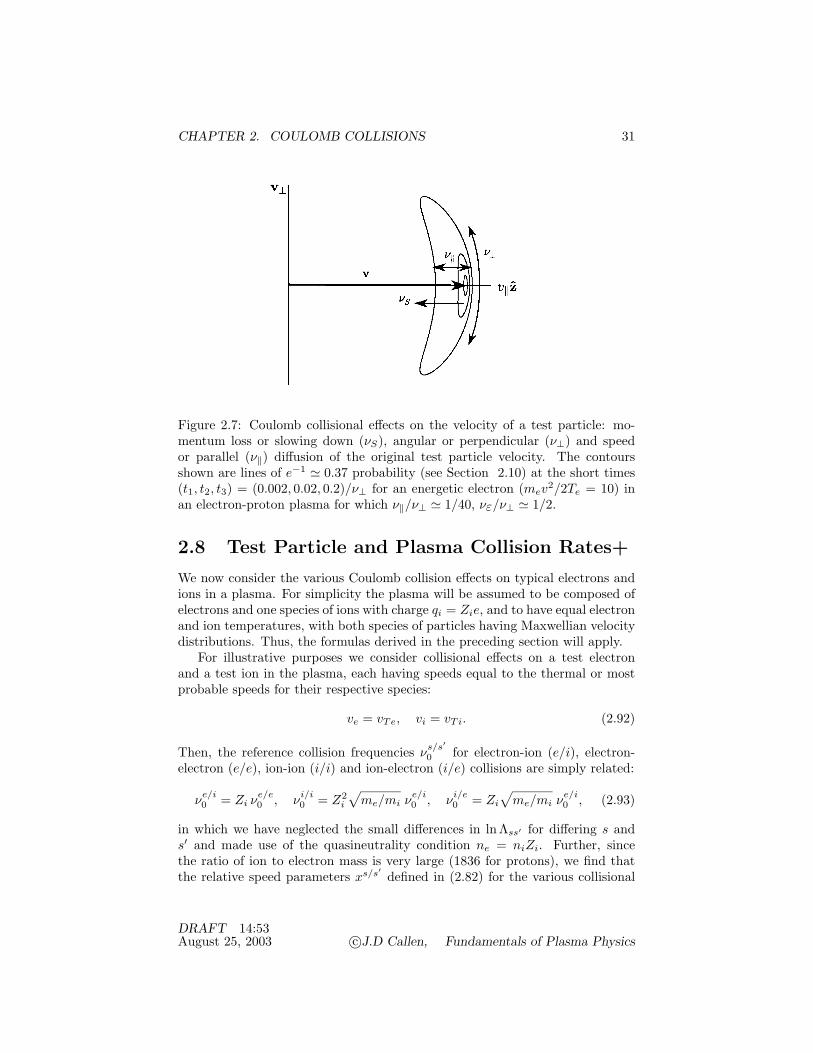
CHAPTER 2. COULOMB COLLISIONS 31
Figure 2.7: Coulomb collisional effects on the velocity of a test particle: mo-mentum loss or slowing down (νS), angular or perpendicular (ν⊥) and speedor parallel (ν‖) diffusion of the original test particle velocity. The contoursshown are lines of e−1 & 0.37 probability (see Section 2.10) at the short times(t1, t2, t3) = (0.002, 0.02, 0.2)/ν⊥ for an energetic electron (mev2/2Te = 10) inan electron-proton plasma for which ν‖/ν⊥ & 1/40, νε/ν⊥ & 1/2.
2.8 Test Particle and Plasma Collision Rates+
We now consider the various Coulomb collision effects on typical electrons andions in a plasma. For simplicity the plasma will be assumed to be composed ofelectrons and one species of ions with charge qi = Zie, and to have equal electronand ion temperatures, with both species of particles having Maxwellian velocitydistributions. Thus, the formulas derived in the preceding section will apply.
For illustrative purposes we consider collisional effects on a test electronand a test ion in the plasma, each having speeds equal to the thermal or mostprobable speeds for their respective species:
ve = vTe, vi = vTi. (2.92)
Then, the reference collision frequencies νs/s′0 for electron-ion (e/i), electron-
electron (e/e), ion-ion (i/i) and ion-electron (i/e) collisions are simply related:
νe/i0 = Zi ν
e/e0 , νi/i
0 = Z2i
√me/mi ν
e/i0 , νi/e
0 = Zi
√me/mi ν
e/i0 , (2.93)
in which we have neglected the small differences in ln Λss′ for differing s ands′ and made use of the quasineutrality condition ne = niZi. Further, sincethe ratio of ion to electron mass is very large (1836 for protons), we find thatthe relative speed parameters xs/s′
defined in (2.82) for the various collisional
DRAFT 14:53August 25, 2003 c©J.D Callen, Fundamentals of Plasma Physics

CHAPTER 2. COULOMB COLLISIONS 32
Figure 2.8: Maxwell integral ψ(x) and related functions.
processes are given by
xe/i =mi
me>> 1, xe/e = 1, xi/i = 1, xi/e =
me
mi<< 1. (2.94)
Thus, we will need both small and large argument expansions of the Maxwellintegral ψ(x) and its derivative ψ′(x), as well as evaluation of them at theparticular value of unity.
The behavior of ψ(x) and other functions of interest are sketched in Fig. 2.8.For x = 1, we have ψ = 0.4276, ψ′ = 0.4151 and ψ+ψ′−ψ/2x = 0.6289. Smalland large argument expansions of interest in evaluating νS , ν⊥, ν‖, and νε are:
x << 1
ψ(x) & (4x3/2/3√π )(1 − 3x/5 + 3x2/14 − · · · ),
ψ′ = (2√
x e−x/√π ) & (2x1/2/
√π)(1 − x + x2/2 − · · · ),
ψ + ψ′ − ψ/2x & (4x1/2/3√π )(1 − x/5 + 3x2/70 − · · · ),
(2.95)
x >> 1
ψ(x) & 1 − (2√
x e−x/√π )(1 + 1/2x − 1/4x2 + · · · ),
ψ′(x) = 2√
x e−x/√π,
ψ + ψ′ − ψ/2x & 1 − 1/2x + (e−x/√π x3/2)(1 − 1/x + · · · ).
(2.96)
Using only the lowest order of these approximations in (2.87)–(2.88), we findthe relationships between various collisional processes listed in Table 2.1. Therates are all referred to the electron-ion collision frequency νe/i
0 , which is the
DRAFT 14:53August 25, 2003 c©J.D Callen, Fundamentals of Plasma Physics

CHAPTER 2. COULOMB COLLISIONS 33
Table 2.1: Relative Coulomb collision rates for thermal speed test electrons andions in a Maxwellian plasma with Te = Ti.
e/i e/e i/i i/e
slowingdown νs/s′
S / νe/i0 1 0.86/Zi 0.86Z2
i
√me
mi0.75Zi
me
mi
perpendiculardiffusion νs/s′
⊥ / νe/i0 2 1.26/Zi 1.26Z2
i
√me
mi1.50Zi
me
mi
speeddiffusion νs/s′
‖ / νe/i0
me
mi0.43/Zi 0.43Z2
i
√me
mi0.75Zi
me
mi
energyloss νs/s′
ε / νe/i0 2
me
mi0.03/Zi 0.03Z2
i
√me
mi− 0.75Zi
me
mi
same as the Lorentz collision frequency in (2.14). The νe/iS and νe/i
⊥ componentsof the first (e/i) column are the same as those given by the Lorentz collisionmodel [cf., (2.13) and (2.19)]. All the other electron processes indicated in thetable arise from the finite mass ratio between the electrons and ions, and the factthat the background particles are in motion. Note that in this general collisionmodel the electron-ion parallel (speed) diffusion (νe/i
‖ ) and energy loss (νe/iε )
are of order me/mi << 1 compared to the Lorentz collision model processes —because of the inefficiency of energy transfer in collisions of particles with verydisparate masses.
From Table 2.1 we see that the various collisional processes naturally splitinto three groups of rates: νe/i
0 , Z2i
√me/mi ν
e/i0 , and Zi(me/mi) ν
e/i0 . The
fastest of these rates is the Lorentz collision rate; however, all the electron-electron collisional processes also occur at roughly the same rate and so shouldalso be taken into account in investigations of electron collisional processes. (Theelectron-electron collision processes are small in a plasma where the ions all havehigh charge states Zi >> 1 since then νe/i
0 = Zi νe/e0 >> νe/e
0 .) Physically, onthis fastest time scale of 1/νe/i
0 , electron momentum is relaxed by collisionson both electrons and ions, and the electrons relax within themselves throughall the processes. The electron-electron collisions relax the electrons toward aMaxwellian distribution (see Chapter 11). On the next lower rate or longertime scale — by a factor of order
√mi/me
>∼ 43 >> 1 — ion-ion collisionsrelax the ions toward a Maxwellian distribution. Finally, on the longest timescale, which is a factor of about mi/me
>∼ 1836 >> 1 slower than 1/νe/i0 , there
is energy transfer between the electrons and ions, and ion momentum loss to theelectrons. [The energy loss rate νi/e
ε is negative here because we are evaluating
DRAFT 14:53August 25, 2003 c©J.D Callen, Fundamentals of Plasma Physics

CHAPTER 2. COULOMB COLLISIONS 34
it for a test particle whose energy is below the average particle energy in theplasma, mv2/2 = 3T/2 — see (??)].
Next, we consider the overall plasma electron and ion species collisionalrelaxation rates. First, we consider the temperature equilibration rate for aMaxwellian distribution of test particles of species s colliding with a Maxwelliandistribution of background particles s′. Multiplying the νs/s′
ε defined in the lastline of (2.88) by an isotropic Maxwellian velocity distribution of test particles sin the form given in (2.76) and using the first property of ψ given in (2.80) tointegrate the ψ contribution to νε by parts once, we find
32ns
dTs
dt= − νs/s′
ε ns(Ts − Ts′), (2.97)
where
nsνs/s′ε = ns
ms
ms′
[4√πνs/s′0 (vTss′)
]= ns′ νs′/s
ε =4√π
4π nsns′q2sq2
s′ ln Λss′
4πε02msms′v3Tss′
,
(2.98)
is the average energy density exchange rate between the species in which
vTss′ ≡ [2(Ts/ms + Ts′/ms′)]1/2 =√
v2Ts + v2
Ts′ (2.99)
is the appropriate mean thermal velocity for a combination of test and back-ground particles, both with Maxwellian distributions. From the equality ofnsν
s/s′ε and ns′ νs/s′
ε , it is obvious that
nsdTs
dt= −ns′
dTs′
dt, (2.100)
as required by energy conservation — energy lost from the test particle species isgained by the (dissimilar) background species with which it suffers Coulomb col-lisions. For a couple of applications of these temperature equilibration formulassee Problems 2.35 and 2.36.
For the special case of the electron-ion plasma we have been considering, ifwe assume Te/me >> Ti/mi (vTe >> vTi), (2.97) becomes [cf., (2.38)]
32ne
dTe
dt= − νe/i
ε ne(Te − Ti) = − 3me
mineνe(Te − Ti) ≡ −Qi. (2.101)
In the last expression we have used the νe defined in (2.17). The relevant formulafor the electron-ion energy transfer rate νe/i
ε in a plasma with impurities (seeProblem 2.37) was given previously in (2.49) and (2.50).
Finally, we calculate the momentum relaxation rate for two Maxwellian dis-tributions of particles that are drifting (flowing) slowly relative to each otherwith velocity V ≡ Vs − Vs′ , assuming |V| << vTss′ . In the rest frame of thebackground particles (s′), the drifting test particle (s) distribution function canbe written as in (2.15):
DRAFT 14:53August 25, 2003 c©J.D Callen, Fundamentals of Plasma Physics
CHAPTER 2. COULOMB COLLISIONS 35
fs(v) = ns
(ms
2πTs
)3/2
exp(− ms|v − V|2
2Ts
)& nse−v2/v2
T s
π3/2v3Ts
[1 +
2v ·Vv2
Ts
+ · · ·]
. (2.102)
Multiplying the momentum loss rate formula in the first line of (2.88) by thisdistribution function and integrating over velocity space, again integrating onceby parts and using the first relation in (2.80), we find
msnsdVs
dt= − νs/s′
S msns(Vs − Vs′), (2.103)
where
msnsνs/s′S = msns
[4
3√π
ms
mss′νs/s′0 (vTss′)
]=
43√π
4π nsns′q2sq2
s′ ln Λss′
4πε02mss′v3Tss′
(2.104)
is the average momentum density exchange rate between the s and s′ species ofparticles, and vTss′ is the average thermal velocity defined in (2.99). From thesymmetric form of msnsν
s/s′S in terms of the species labels s and s′, it is clear
that the momentum lost from the s species is gained by the s′ species and thusmomentum is conserved in the Coulomb collisional interactions between the twospecies of particles: msnsdVs/dt = −ms′ns′dVs′/dt.
Specializing again to an electron-ion plasma and assuming as usual thatvTe >> vTi, we find that (2.103) and (2.104) reduce to [cf., (2.34)]
menedVe
dt= −meneνe(Ve − Vi) ≡ Re, (2.105)
where
νe = νe/iS =
43√πνe/i0 (vTe) =
4√
2π neZie4 ln Λ
4πε02 3 m1/2e T 3/2
e
≡ 1τe
. (2.106)
This electron momentum relaxation rate is the same as that obtained in (2.17)for the Lorentz collision model and shows that the fundamental Maxwellian-averaged electron-ion collision frequency νe is in fact νe/i
S . Electron-electroncollisions do not contribute to the momentum relaxation process because theyare momentum conserving for the electron species as a whole. Note also thatthe collisional momentum relaxation process acts on the difference between theelectron and ion flow velocities. Thus, the net effect of Coulomb collisions is torelax the electron flow to the ion flow velocity. Finally, the relevant formula forthe electron-ion collisional “slowing down” rate νe/i
S in a plasma with impurities(see Problem 2.38) was given in (2.44).
For the slightly fictitious case of two ion species with charge qi = Zie thathave equal temperatures but are drifting relative to each other with velocity V,the ion momentum relaxation rate is given by
DRAFT 14:53August 25, 2003 c©J.D Callen, Fundamentals of Plasma Physics

CHAPTER 2. COULOMB COLLISIONS 36
minidVdt
= −miniνiV, (2.107)
where [cf., (2.36)]
νi = νi/iS =
4√π niZ4
i e4 ln Λ
4πε02 3 m1/2i T 3/2
i
≡ 1τi
. (2.108)
As can be anticipated from the νi/iS entry in Table 2.1, this momentum relaxation
rate is a factor of order Z2i
√me/mi slower than that for electrons. Also, the
ion-electron collisional effects due to νi/eS have been neglected in the average ion
momentum loss rate because they are a factor of order√
me/mi smaller thanthe ion-ion collisional effects. The numerical factor in (2.108) is
√2 smaller than
that in (2.106) because of the rest mass and average thermal velocity factorsfor this equal mass case. Finally, the relevant formula for the ion-ion collisional“slowing down” rate νi/i
S in a plasma with impurities (see Problem 2.39) wasgiven in (2.46).
2.9 Fast Ion Thermalization+
In attempting to heat plasmas one often introduces “fast” ions (through ab-sorption of energetic neutrals, from radiofrequency wave heating, or directly asenergetic charged fusion products such as α particles), which have speeds in-termediate between the ion and electron thermal speeds. These fast ions heatthe plasma by transferring their energy to the background plasma electrons andions during the Coulomb collisional slowing down process. This fast ion slowingdown and energy transfer process will now be considered in some detail.
For simplicity we consider an electron-hydrogenic (proton, deuteron or triton— mi = 1, 2 or 3 but Zi = 1) background plasma in which both species havea Maxwellian velocity distribution. The electron and ion temperatures will beassumed to be unequal, but comparable in magnitude. The fast or test ionwill be allowed to have a mass (mf ) and charge (qf = Zfe) different fromthe background ions. Because the fast ion speed is intermediate between theelectron and ion thermal speeds, the relative speed parameters in (2.82) for thefast ion-ion (f/i) and fast ion-electron (f/e) collisions are given by
xf/i =miv2
2Ti=
v2
v2Ti
>> 1, xf/e =mev2
2Te=
v2
v2Te
<< 1, (2.109)
in which v is the fast ion speed. Further, the reference collision frequencies νf/s′0
are equal for the electron-hydrogenic ion background plasma:
νf/i0 = νf/e
0 . (2.110)
Using the approximations (2.109) in (2.95) and (2.96), we find that the fastion transfers energy to the plasma electrons and ions at the rates defined in the
DRAFT 14:53August 25, 2003 c©J.D Callen, Fundamentals of Plasma Physics
CHAPTER 2. COULOMB COLLISIONS 37
last equation in (2.88), which are given to lowest significant order by
νf/iε & 2
mf
miνf/i0 , (2.111)
νf/eε & 2
mf
me
4(xf/e)3/2
3√π
νf/e0 = 2
mf
me
43√π
v3
v3Te
νf/e0 . (2.112)
From the definition of νf/s′0 in (2.87) we see that it depends on v−3. Thus,
νf/iε also depends on v−3. However, νf/e
ε is independent of the fast ion speedv — because the appropriate relative speed for fast ion-electron collisions withvTe >> v is the electron thermal speed.
Adding together the fast ion energy losses via collisions with backgroundplasma ions and electrons, the total fast ion energy loss rate becomes
dεdt
= −(νf/eε + νf/i
ε
)ε, (2.113)
in which
ε = mfv2/2 (2.114)
is the instantaneous fast ion energy. Since νf/eε is independent of the fast ion
energy, it is convenient to define a fast ion slowing down time τS in terms of it:
τS ≡ 2
νf/eε
& 1
νf/eS
=mf
me
4πε02 3 m1/2e T 3/2
e
(4√
2π) neZ2fe4 ln Λ
=(
mf
me
)1νe
. (2.115)
Here, the approximate equality to 1/νf/eS follows because for mf/me >> 1 the
fast ions are not significantly scattered by the electrons; thus, they lose energyto the plasma electrons at twice the rate they lose momentum to them. The rateof transfer of fast ion energy to plasma ions can be referenced to the transferrate to the electrons in terms of a critical energy εc ≡ mfv2
c/2 as follows:
νf/iε
νf/eε
=(εc
ε
)3/2
=v3
c
v3, (2.116)
where
εc ≡ mfv2c
2= Te
[3√π
4
√mf
me
mf
mi
]2/3
& 14.8 Te
(mf
m1/3p m2/3
i
)(2.117)
in which mp is the proton mass. (For the appropriate modifications when mul-tiple species of ions are present, see Problems 2.40 and 2.50.) In terms of thiscritical energy, (2.113) can be written as
dεdt
= − 2 ετS
[1 +
(εc
ε
)3/2]
. (2.118)
DRAFT 14:53August 25, 2003 c©J.D Callen, Fundamentals of Plasma Physics

CHAPTER 2. COULOMB COLLISIONS 38
Figure 2.9: Fast ion energy transfer rate versus energy ε. The energy transferis primarily to electrons for ε > εc, but to ions for ε < εc.
The fast ion energy transfer rates as a function of energy are illustrated in Fig.2.9. For fast ion energies greater than εc the energy transfer is primarily toelectrons, while for ε < εc it is primarily to ions.
Since (2.118) applies for all fast ion speeds between the electron and ionthermal speeds, it will be valid for all fast ion energies during the thermalizationprocess. Thus, its solution will give the fast ion energy as a function of time as ittransfers its energy to the background plasma. To solve (2.118) it is convenientto convert it to an equation for the fast ion speed v ≡ √
2ε/mf , for which itbecomes
dv
dt= − v
τS
[1 +
v3c
v3
], (2.119)
vc ≡√
2 εc
mf=
[3√π
4me
mi
]1/3
vTe. (2.120)
Multiplying (2.119) by v2 and integrating over time from t = 0 where the initialfast ion speed will be taken to be v0 to the current time t where it has speed v(assumed > vTi), we obtain
t =τS
3ln
(v30 + v3
c
v3 + v3c
), (2.121)
orv3(t) = (v3
0 + v3c ) e−3t/τS − v3
c . (2.122)
The fast ion energy ε(t) = mfv2(t)/2 during the slowing down process can bereadily obtained from this last result.
DRAFT 14:53August 25, 2003 c©J.D Callen, Fundamentals of Plasma Physics

CHAPTER 2. COULOMB COLLISIONS 39
E/Ec
t/τs
0 0.5 1.1
.3
1
3
10
Figure 2.10: Decay of fast ion energy ε versus time during thermalization intoa background plasma for various initial ratios of ε to the critical energy εc.
The decay of the fast ion energy with time is illustrated in Fig. 2.10. Notethat for initial energies much greater than the critical energy εc the fast ionenergy decays exponentially in time at a rate 2/τS = νf/e
ε due to collisions withelectrons, as is apparent from (2.118). However, when the energy drops belowεc the energy transfer is predominantly to the ions and the fast ion energydecays much faster than exponentially. The total lifetime for thermalization (tov & vTi << vc) of the fast ion into the background plasma ions is
τf & (τS/3) ln [1 + (ε0/εc)3/2] = (τS/3) ln [1 + v30/v3
c ]. (2.123)
A couple of applications of these fast ion slowing down effects and formulas aredeveloped in Problems 2.41–2.42.
Next, we calculate the fraction of the fast ion energy that is transferred tothe background plasma electrons and ions over the entire fast ion slowing downprocess. Since in many plasma situations the fast ions are also susceptible toother, direct loss processes such as charge-exchange, we introduce a probabilityexp(−t/τcx) that the fast ion will remain in the plasma for a time t againstcharge-exchange losses at rate 1/τcx. Then, the fraction Ge of the total fastion energy ε0 ≡ mfv2
0/2 transferred to the electrons during the thermalizationprocess is given by
Ge ≡ 1ε0
∫ τf
0dt
(− dε
dt
)νf/eε e−t/τcx
νf/eε + νf/i
ε=
2v20
∫ v0
0
v3 v dv
v3 + v3c
[v3 + v3
c
v30 + v3
c
]τS/3τcx
. (2.124)
Similarly, the fraction Gi of fast ion energy transferred to the ions is (for thesimpler case where τcx → ∞, see also the form given in Problem 2.43)
Gi ≡ 1ε0
∫ τf
0dt
(− dε
dt
)νf/iε e−t/τcx
νf/eε + νf/i
ε=
2v20
∫ v0
0
v3c v dv
v3 + v3c
[v3 + v3
c
v30 + v3
c
]τS/3τcx
. (2.125)
DRAFT 14:53August 25, 2003 c©J.D Callen, Fundamentals of Plasma Physics

CHAPTER 2. COULOMB COLLISIONS 40
0.1 0.2 0.5 1 2 5 100
0.2
0.4
0.6
0.8
1
01
310
0
1
3
10
τsτcx
____ =
electrons
ions
Eo/Ec
Gi,!Ge
Figure 2.11: Fraction of the fast ion energy ε0 that is transferred to the back-ground plasma electrons (Ge) and ions (Gi) as a function of the ratio of theinitial energy ε0 to the critical energy εc. The variation with the parameterτS/τcx indicates the influence of direct fast ion losses (at rate 1/τcx) during thethermalization process.
The fraction of fast ion energy lost due to charge-exchange is 1 − Gi − Ge.However, a portion of this energy may be absorbed in the plasma if some of thefast neutrals produced by charge-exchange are reabsorbed before they leave theplasma.
The variation of the fractions Ge, Gi of fast ion energy transferred to plasmaelectrons and ions during the thermalization process are illustrated in Fig. 2.11.Note that the integrated fractions become equal for ε0
<∼ 2.5 εc, which is abovethe value of ε0 & εc where the instantaneous energy transfer rates are equal.Also, charge-exchange losses become significant for τS/τcx >∼ 1, and can greatlydiminish the fast ion energy transfer to the plasma for τS/τcx >> 1. For sometypical applications of fast ion slowing down and energy transfer processes andtheir effects on plasmas, see Problems 2.44–2.47.
In addition to energy loss, the fast ions experience perpendicular and paralleldiffusion in velocity space during their thermalization. The relative importanceof the various Coulomb collision processes on the fast ion for the conditionsgiven in (2.109) are indicated in Table 2.2. From this table we see that forε >> εc the momentum and energy losses by the fast ions to the electronsare the dominant processes because then the velocity space diffusion effectsindicated by ν⊥, ν‖ are small. However, for ε < εc the fast ions lose energyprimarily to the background ions and their perpendicular or angular diffusionrate in velocity space becomes equal to their energy loss rate. For some typicalapplications of fast ion scattering processes and their effects on plasmas, seeProblems 2.48–2.50.
The energy or speed diffusion process indicated by ν‖ is negligible untilthe fast ion energy is reduced to approximately the ion temperature in the
DRAFT 14:53August 25, 2003 c©J.D Callen, Fundamentals of Plasma Physics

CHAPTER 2. COULOMB COLLISIONS 41
Table 2.2: Relative Coulomb collision rates for fast ions with vTi << v << vTe
slowing down in a plasma with Maxwellian electrons and ions (εc ∼ 14.8 Te).f/i f/e
slowingdown νf/s′
S / νf/e0
(1 +
mf
mi
)mf
me
43√π
(v
vTe
)3
=(
εεc
)3/2
perpendiculardiffusion νf/s′
⊥ / νf/e0 2
83√π
(v
vTe
)<< 1
speeddiffusion νf/s′
‖ / νf/e0
Ti
mfv2/2<< 1
43√π
(v
vTe
)<< 1
energyloss νf/s′
ε / νf/e0 2
mf
mi
mf
me
83√π
(v
vTe
)3
= 2(
εεc
)3/2
background plasma. Since the energy diffusion process is thus negligible duringthe fast ion thermalization process, and the perpendicular diffusion has no effecton the energy transfer rates, our characterization of the fast ion slowing downprocess as one of a monotonic decrease in the fast ion energy is a reasonablyaccurate one. A kinetic description that allows for pitch-angle (ϑ) scatteringalong with the fast ion energy slowing down is developed in Section 11.4.
2.10 Evolution of Velocity of a Test Particle+
To further illustrate the Coulomb collision effects, we examine the collisionalevolution of the velocity of a test particle for short times where the velocitychanges are small. The test particle will be assumed to be colliding with aplasma whose components have Maxwellian distributions. Thus, the results ofSection 2.7 will be applicable.
A test particle of species s will be taken to have an initial velocity v0 in theez or parallel direction (cf., Fig. 2.4). Integrating the first equation of (2.88)over a short time t >> ∆t (for validity of the dynamical friction and velocitydiffusion coefficients), we find that the mean parallel or ez component of thetest particle velocity after a time t is
v‖ = v0(1 − νSt), νS = νsS ≡
∑s′
νs/s′S (v0). (2.126)
This result is valid for νSt << 1 and indicates the monotonic decrease in testparticle momentum due to Coulomb collisons. Similarly, the test particle energyafter a short time t can be obtained directly by integrating the last equation of
DRAFT 14:53August 25, 2003 c©J.D Callen, Fundamentals of Plasma Physics
CHAPTER 2. COULOMB COLLISIONS 42
(2.88) over time:
12mv2 =
12mv2
0(1 − νεt), νε = νsε ≡
∑s′
νs/s′ε (v0). (2.127)
Thus, the average test particle speed v, which will be used below, will be definedby
v ≡√
v2 & v0(1 − νεt/2). (2.128)
Similar to (2.126), these formulas are only valid for νεt << 1.The angular (perpendicular) velocity and speed (parallel) diffusion processes
in velocity space indicated by ν⊥ and ν‖ have to be treated differently. Becausethese Coulomb collision effects are random in character and diffusive, they leadto a Gaussian probability distribution P (v−v0) of the velocity about the initialtest particle velocity v0. Since the diffusion results from purely random pro-cesses, we can anticipate (and will derive in Chapter 11) that this probabilitydistribution will be Gaussian and of the form:
P (v − v0) =1
2π v2
(e−ϑ2/2σ2
⊥
σ2⊥
) (e−(v−v)2/2σ2
‖√2π σ‖
). (2.129)
Here, ϑ2 ≡ [arcsin−1(v⊥/v)]2 & (v2x + v2
y)/v2 and v is as was defined in (2.128).Taking velocity-space averages of various quantities A(v) over this probabilitydistribution [A ≡ ∫ ∞
0 2πv2 dv∫ π0 sinϑ dϑ P (v − v0)A(v)], we find that while
the average of the diffusive deflections vanish [vx = vy = 0, v‖ − v‖ = 0], thediffusive spreads in the perpendicular and parallel (to v0) directions are
v2 − v20 & v2
⊥ = v2x + v2
y = 2σ2⊥v2
0 , (v‖ − v0)2 = (v‖ − v‖)2 = σ2‖. (2.130)
To determine the probability variances σ⊥ and σ‖ for the diffusive Coulombcollisional processes, we integrate the middle two equations in (2.88) over a shorttime t, and obtain
v2⊥ = (ν⊥t) v2
0 , ν⊥ = νs⊥ ≡
∑s′
νs/s′⊥ (v0) (2.131)
(v‖ − v‖)2 = (ν‖t) v20 , ν‖ = νs
‖ ≡∑s′
νs/s′
‖ (v0). (2.132)
Comparing (2.130), (2.132) and (2.132), we see that for Coulomb collisions
σ⊥ =√ν⊥t/2, σ‖ =
√ν‖t v0. (2.133)
The relative collisional spreads (half-widths in velocity space to points wherethe probability distribution drops to e−1/2 & 0.61 of its peak value) of the testparticle velocity in the directions perpendicular and parallel (i.e., for speed orenergy diffusion) relative to its initial velocity v0 are given by
δϑ & δv⊥/v0 ≡ σ⊥ =√ν⊥t/2, δv/v0 ≡ σ‖/v0 =
√ν‖t. (2.134)
DRAFT 14:53August 25, 2003 c©J.D Callen, Fundamentals of Plasma Physics

CHAPTER 2. COULOMB COLLISIONS 43
Note that in comparing the perpendicular diffusion factor in (2.129) for whichσ⊥ =
√ν⊥t/2 with the perpendicular diffusion in the Lorentz model as given
in (2.21), we need to realize that ν⊥ = 2 ν and hence that σ⊥ =√νt for
the Lorentz collision model. These formulas indicate that, even for very hightemperature plasmas with nλ3
D >> 1 where the Coulomb collision rates are veryslow, only a short time is required to diffuse the test particle velocity througha small δv << v0. For example, as indicated in (2.20), the time required todiffuse a particle’s velocity through a small angle ϑ & δv⊥/v0 << 1 is onlyt & 2ϑ2/ν⊥ << 1/ν⊥ [or, t & ϑ2/ν << 1/ν for the Lorentz collision model].Thus, because of the diffusive nature of Coulomb collisions, it takes much lesstime to scatter through an angle ϑ << 1 in velocity space than it does to scatterthrough 90 (ϑ ∼ 1). The various diffusive collisional effects are illustrated inFig. 2.7. There, the contours shown indicate where the probability distributionP in (2.129) is equal to e−1 & 0.37 of its peak value for ν⊥t = 0.002, 0.02, 0.2,for a typical set of test particle parameters.
The change in the average energy mv2/2 can also be obtained using (2.126),(2.130) and (2.133). This procedure yields, correct to first order in νt << 1,
12mv2 = 1
2m[v2‖ + v2
⊥]
= 12m
[v‖2 + 2(v‖ − v‖)v‖ + (v‖ − v‖)2 + v2
⊥]
& 12m[v2
0(1 − 2νSt) + σ2‖ + 2σ2
⊥] = 12mv2
0 [1 − (2νS − ν⊥ − ν‖)t].
This result is the same as (2.127) because of the relation between the variouscollisional processes given in (2.89).
The formulas developed in this section also provide a basis for a probablistic(Monte Carlo) numerical approach for inclusion of Coulomb collision effects inother plasma processes such as single particle trajectories. Thus far we havefound that after a short time t a test particle’s velocity and speed decreaseaccording to (2.126) and (2.128). However, the test particle also acquires adiffusive spread in the perpendicular and parallel directions as given by (2.129)with the spreads (variances) defined in (2.133). Further, the velocity spacelatitudinal angle ϕ [cf., (2.1)] is completely randomized by successive individualCoulomb collisions — in a time scale t >> ∆t. Hence, defining a randomvariable ξ to be evenly distributed between 0 and 1, and independent randomvariables η1, η2 sampled from a normal probability distribution [i.e., Gaussiansuch as indicated in the σ‖ part of (2.129)] with zero mean and a mean squareof unity (i.e., η1 = η2 = 0 but η2
1 = η22 = 1), we find that the total velocity
vector v after a short time t (νt << 1) can be written as
v = v0 (1 − νεt/2)[ez ( 1 + η1
√ν‖t ) + |η2|
√ν⊥t/2 (ex cos 2πξ + ey sin 2πξ)
].
(2.135)
This form can be used to develop a Monte Carlo algorithm for advancingthe test particle velocity v taking into account the Coulomb collision dynam-ical friction and velocity space diffusion effects occurring over the short timet << 1/ν. Since (2.135) implies a change in the velocity of the test particle,
DRAFT 14:53August 25, 2003 c©J.D Callen, Fundamentals of Plasma Physics

CHAPTER 2. COULOMB COLLISIONS 44
in order to preserve the momentum and energy conserving properties of theelastic Coulomb collision process, the velocity of the background particles mustalso change, at least on average. Hence, in order to develop a complete MonteCarlo-based Coulomb collision operator we should consider simultaneously botha test and a background particle. Then, the change in velocity δv ≡ v − v0
for the test particle is determined from (2.135), and that for the backgroundparticle is given by δv′ = − (ms/ms′)δv — see (2.59).
REFERENCES AND SUGGESTED READING
The basic Coulomb collision processes were first worked out in the analogous con-text (see Problem 2.9) of the gravitational interaction of stars:
Chandrasekhar, Principles of Stellar Dynamics (1942).
S. Chandrasekhar, Rev. Mod. Phys. 15, 1 (1943).
A comprehensive application to Coulomb collisions in a plasma was first presented in
Spitzer, Physics of Fully Ionized Gases (1962).
The most general development of the dynamical friction and velocity diffusion coeffi-cients for a plasma in terms of the Rosenbluth potentials originated in the paper
M.N. Rosenbluth, W. MacDonald and D. Judd, Phys. Rev. 107, 1 (1957).
The most comprehensive treatments of the Coulomb collision effects on test particlesin a plasma are found in
B.A. Trubnikov, “Particle Interactions in a Fully Ionized Plasma,” in Reviews ofPlasma Physics, M.A. Leontovich, ed. (Consultants Bureau, New York, 1965),Vol. I, p. 105.
D.V. Sivukhin, “Coulomb Collisions in a Fully Ionized Plasma,” in Reviews ofPlasma Physics, M.A. Leontovich, ed. (Consultants Bureau, New York, 1966),Vol. IV, p. 93.
A brief, but very useful summary of the important Coulomb collision formulas in thischapter is given in
Book, NRL Plasma Formulary (1990), p. 31.
A book devoted almost entirely to the subject of Coulomb collision effects in a plasmawith numerous examples worked out is
Shkarofsky, Johnston and Bachynski, The Particle Kinetics of Plasmas (1966).
Also, most books on plasma physics have chapters devoted to discussions of Coulombcollision effects. Among the most descriptive and useful are those in
Spitzer, Physics of Fully Ionized Gases (1962), Chapter 5
Rose and Clark, Plasmas and Controlled Fusion (1961), Chapter 8.
Schmidt, Physics of High Temperature Plasmas (1979), Chapter 11.
Krall and Trivelpiece, Principles of Plasma Physics (1973), Chapter 6.
Golant, Zhilinsky and Sakharov, Fundamentals of Plasma Physics (1980), Chap-ter 2.
The original theory of runaway electrons was developed in
H. Dreicer, Proceedings of the Second United Nations International Conferenceon the Peaceful Use of Atomic Energy (United Nations, Geneva, 1958), Vol. 31,p. 57. See also, Phys. Rev. 115, 238 (1959).
DRAFT 14:53August 25, 2003 c©J.D Callen, Fundamentals of Plasma Physics

CHAPTER 2. COULOMB COLLISIONS 45
The thermalization of a fast ion in a Maxwellian plasma was first developed in
D.J. Sigmar and G. Joyce, Nuclear Fusion 11, 447 (1971).
T.H. Stix, Plasma Physics 14, 367 (1972).
Inclusion of charge-exchange loss and geometry effects on neutral-beam-injected fastions are discussed in
J.D. Callen, R.J. Colchin, R.H. Fowler, D.G. McAlees and J.A. Rome, “NeutralBeam Injection into Tokamaks,” Plasma Physics and Controlled Nuclear FusionResearch 1974 (IAEA, Vienna, 1975), Vol. I, p. 645.
The Monte Carlo computational approach to including Coulomb collisional effects hasbeen developed primarily in the context of investigating transport processes in
R. Shanny, J.M. Dawson and J.M. Greene, Phys. Fluids 10, 1281 (1967).
K.T. Tsang, Y. Matsuda and H. Okuda, Phys. Fluids 18, 1282 (1975).
T. Takizuka and H. Abe, J. Comput. Phys. 25, 205 (1977).
A.H. Boozer and G. Kuo-Petravic, Phys. Fluids 24, 851 (1981).
PROBLEMS
2.1 Consider the length scales relevant for electron Coulomb collision processes in atypical university-scale magnetic fusion plasma experiment that has ne = 2×10¹³
cm−3 and Te = Ti = 1 keV. Calculate: a) the distance of closest approach bmin;b) the average interparticle spacing; c) the maximum interaction distance bmax;and d) the average collision length λe = vTe/νe for electrons in this plasma.What is the ratio of each of these lengths to the mean interparticle spacing? /
2.2 Consider the length scales relevant for electron Coulomb collision processes ina laser-produced electron-proton plasma that has ne = 1029 m−3 and Te = Ti
= 1 keV. Calculate: a) the distance of closest approach bmin; b) the averageinterparticle spacing; c) the maximum interaction distance bmax; and d) theaverage collision length λe = vTe/νe for electrons in this plasma. What is theratio of each of these lengths to the mean interparticle spacing? /
2.3 Estimate the time scales relevant for electron Coulomb collision processes in theearth’s ionosphere at a point where ne = 1012 m−3, Te = 1 eV. For simplicity,use a Lorentz collision model and assume the ions have Zi = 1 and Ti " Te.Calculate the times for: a) a typical Coulomb interaction at the average inter-particle spacing; b) an electron to traverse the Debye shielding cloud; and c) theaverage electron collision time τe = 1/νe. How long (or short) are each of thesetimes compared to the “plasma period” ω−1
pe ? /
2.4 a) Show that for a Lorentz collision model an electron with an initial velocity v0
loses momentum exponentially in time at a decay rate given by ν(v0). b) Whatis the electron energy after its momentum is totally depleted? c) Calculate thedistance the electron travels in its original direction of motion while losing itsmomentum. d) Evaluate the momentum decay rate and distance the electrontravels for a plasma with Zi = 5, ne = 1019m−3, Te = Ti = 100eV , and aninitial electron “test particle” energy of 1 keV. [Hint: Be careful to distinguishbetween an electron’s velocity (a directional, vector quantity) and its speed (ascalar quantity).] //
2.5 In Section 2.1 we derived the momentum impulse ∆v for a single Coulombcollision in the Lorentz collision model by integrating me(dv/dt) = qeE over an
DRAFT 14:53August 25, 2003 c©J.D Callen, Fundamentals of Plasma Physics

CHAPTER 2. COULOMB COLLISIONS 46
unperturbed “straight-line” trajectory to determine ∆v⊥ and then used ∆v‖ "−∆v⊥ · ∆v⊥/2v. Show that the result for ∆v‖ given in (2.6) can be obtaineddirectly by integrating E[x(t)] along a perturbed electron trajectory x(t) = x+xthat includes the first order effects x due to the E field of the ion on the electrontrajectory. [Hint: First calculate the perturbed velocity v, and then make useof the fact that
∆v‖ = ez · qe
me
∫ ∞
−∞dt E(x + x) =
qe
me
∫ ∞
−∞dt ez ·
[E(x) + x · ∂E
∂x
∣∣∣∣x
+ · · ·]
=e
me
∫ ∞
−∞dt v ·∇
∫ t
−∞dt′ Ez(t
′) =Zie
2
4πε0mev
∫ ∞
−∞dt v‖
t
(b2 + v2t2)3/2.] ///
2.6 Show that the Lorentz collision frequency ν can be derived from the Rutherforddifferential scattering cross-section dσ = (dσ/dΩ)dΩ given in (??) and Prob-lem 2.24. First, show that for the Lorentz collision model the scattering angle ϑis given for typical small-angle Coulomb collisions by ϑ " 2Zie
2/(4πε0mv2b)= 2bcl
min/b, and that the differential scattering cross-section kernal is dσ/dΩ= |(b db dϕ)/(dϕ d cosϑ)| " (b/ϑ)|db/dϑ| = 4(bcl
min)2/ϑ4. Then, determine theeffective cross-section for momentum transfer σm, which is defined by
σm ≡∫
dΩ (dσ/dΩ) (1 − cosϑ).
In performing this integral discuss the maximum, minimum scattering anglesϑmax, ϑmin in terms of the bmin, bmax interaction distances. Finally, show thatν = niσmv yields the Lorentz model collision frequency given in (2.14). ///
2.7 Use the full Rutherford differential scattering cross-section and the procedureoutlined in the preceding problem to give an alternate derivation of the Lorenzcollision frequency that takes into account classical “hard,” or large angle colli-sions; i.e., do not initially assume ϑ << 1. ///
2.8 The Lorentz collision frequency ν can also be determined from the Langevinequation
medvdt
= −meν v + ∆F(t)
in which −meν v is the dynamical friction force, and ∆F(t) is a stochastic force,which for Coulomb collisions is that given by (2.2). Assuming ν is constant intime, use an integrating factor eνt in solving the Langevin equation to determinethe particle velocity v(t) after its initialization to v0 at t = 0. Next, calculatethe ensemble average of the electron kinetic energy as a function of time, andshow that it yields
〈v2(t)〉 " v20 e−2νt +
1 − e−2νt
2ν
∫ ∞
−∞dτ
〈∆F(0) · ∆F(τ)〉m2
e.
Show that for times long compared to the duration of individual Coulomb col-lisions but short compared to the momentum loss collision time (b/v << t <<1/ν), the electron kinetic energy is constant through terms of order νt when
ν ≡ 12m2
ev2
∫ ∞
−∞dτ 〈∆F(0) · ∆F(τ)〉.
DRAFT 14:53August 25, 2003 c©J.D Callen, Fundamentals of Plasma Physics
CHAPTER 2. COULOMB COLLISIONS 47
Thus, ν is proportional to the autocorrelation function of the Coulomb colli-sion force ∆F. Next, show that for Coulomb collisions between electrons anda stationary background of randomly distributed ions this formula yields theLorentz collision frequency given by (2.14). Finally, making use of the equi-librium (νt → ∞) statistical mechanics (thermodynamics) property that forrandom (Brownian) motion due to a stochastic force ∆F the ensemble-averagekinetic energy me〈v2〉/2 of a particle is Te/2, note that this last result yields
ν =me
2 Te
∫ ∞
−∞dτ
〈∆F(0) · ∆F(τ)〉m2
e, fluctuation-dissipation theorem,
which is also related to Nyquist’s theorem for noise in electric circuits. [Hints:a) Here, 〈f〉 ≡ ni
∫d3x f = ni
∫ ∞−∞ dz
∫b db
∫ 2π
0dϕ f ; b) The electron position
for an ion at x = zez at time t = 0 is x = b(ex cosϕ+ ey sinϕ)− (z − vt)ez. ///
2.9 Consider cumulative small-angle collisional interactions of a test star of mass Mt
and velocity v in a galaxy for which the gravitational force between it and groupsof field stars with density nf and mass Mf is given by [cf., (??) in Section A.6]FG = −GMtMf (xt−xf )/|xt−xf |3 — an attracive inverse square law force likethat for Coulomb collisions of oppositely charged particles. Develop a modelfor collisions of this test star with other, background stars and show that thereference gravitational collision frequency analogous to (2.14) is
νG =4πG2nfM2
f
v3ln
[D0u2
G(Mt + Mf )
],
where bmax has been taken to be D0, the mean distance between stars (∼ n−1/3f )
and bmin has been taken to be the minimum interaction distance given by anexpression analogous to that implied by (2.9). Estimate the time in (years) forthe velocity of our sun to scatter through 90, assuming that our sun is a typicalstar in our galaxy which has a mass of 2 × 1030 kg, a velocity of 20 km/s anda mean separation from other stars in our galaxy of 1 parsec (" 3 × 10¹³ km).Will you be concerned about this scattering process in your lifetime? ///
2.10 Estimate the diffusion coefficient D for a Fick’s law representation (Γ = −D∇n)of the particle flux Γ due to electron-ion Coulomb collision effects in an inho-mogeneous plasma as follows. For simplicity, use a Lorentz collision modeland assume the electrons have a density gradient but no temperature gradient.Then, show by balancing the pressure gradient force density −∇pe = −Te∇ne
against the frictional drag induced by Coulomb collisions that D = Te/meνe
= νeλ2e/2. Estimate the magnitude of this diffusion coefficient for the plasma
described in Problem 2.3 and compare the result to the viscous diffusion coeffi-cient for molecules of air at the earth’s surface. Why is the diffusivity of chargedparticles in a plasma so much larger? //
2.11 Estimate the D-D fusion reaction rate (use σfv " 10−17 cm3/s) for a plasmawith Te = Ti = 40 keV, and ne = 1020 m−3. Compare this rate to typicalelectron and ion Coulomb collision rates in this fusion plasma. How many timesdo electrons and ions scatter through 90 during a typical D-D fusion in thisplasma? How far do typical electrons and ions travel in a characteristic fusionreaction time? /
2.12 Consider the angular scattering of a beam of 100 eV electrons introduced intoan Argon laboratory plasma that has Te = 3 eV, Ti = 1 eV, Zi = 3 and an
DRAFT 14:53August 25, 2003 c©J.D Callen, Fundamentals of Plasma Physics

CHAPTER 2. COULOMB COLLISIONS 48
electron density ne = 1019 m−3. Using the Lorentz collision model, estimatethe distance over which the beam electrons are: a) scattered through an angleof 6; b) scattered via small angle collisions through an angle of about 90; andc) deflected 90 via hard collisions. Finally, d) estimate the angle ∆ϑ throughwhich a beam electron is scattered in a typical Coulomb interaction when theimpact parameter b is given by the mean interparticle spacing of ions. //
2.13 Determine the energy at which electrons “run away” in response to an electricfield in an impure plasma as follows. Assume that a nearly Maxwellian plasma(Ti ∼ Te) is composed of electrons and various species of ions with charge Zi,for which charge neutrality requires ne =
∑i niZi. Calculate the frictional
drag force on electrons in the high energy tail (mev2/2 >> Te) of the electron
distribution. Show that the energy at which electrons run away is given by(2.27) with Zi now replaced by the Zeff defined in (2.43). Also, estimate thefraction of electrons that are runaways for |E|/ED = 0.1 and Zeff = 2. //
2.14 As electrons become relativistic (v → c) the dynamical friction force decreasesless rapidly than the 1/v2 indicated in (2.25) and Fig. 2.6. In fact, it becomesnearly constant for γ ≡ (1 − v2/c2)−1/2 >> 1. Then, if the electric field isweak enough, there are no runaway electrons. Determine the dynamical frictionforce on relativistic electrons in a nonrelativistic plasma composed of electronsand ions of charge Zi as follows. First, show that the change in perpendicularmomentum (p ≡ γmev) in a single Coulomb collision is given by
∆p⊥ = − 2Zie2
4πε0bv (ex cosϕ+ ey sinϕ).
Next, use the relativistic form of the total particle energy (ε =√
m2ec4 + p2c2)
to show that for Coulomb scattering (constant energy) collisions between highenergy electrons and background electrons or ions of mass mi the change inparallel momentum is
∆p‖ " − ∆p⊥ · ∆p⊥2p
[1 + γ
me
mi
].
Show that the frictional force induced by Coulomb collisions of the high energyelectron with the background plasma is thus
〈F‖〉 " − 4π nee4 ln Λ
4πε02mev2
(1 +
1 + Zi
γ
)Finally, show that for a weak electric field satisfying
|E|/ED < 2Te/(mec2)
no runaway electrons will be produced in the plasma. ///+
2.15 Estimate the electric field strength at which the entire electron distributionfunction runs away as follows. First, assume the ions are at rest and theelectrons are described by a shifted Maxwellian as defined in (2.102). Then,transform to the electron rest frame where V = 0. In this frame the ions allhave a velocity −V. Show that the frictional force on a test ion is given by(mi/me) miν
i/e0 (v)ψi/e(x)V in which xi/e = V 2/v2
Te. Find the maximum ofthis frictional force as a function of V/vTe (cf., Fig. 2.8). Then, use the fact
DRAFT 14:53August 25, 2003 c©J.D Callen, Fundamentals of Plasma Physics

CHAPTER 2. COULOMB COLLISIONS 49
that this frictional force must be equal and opposite to the maximum force onthe electron distribution to estimate the critical electric field strength (in termsof the Dreicer field) for total electron runaway. Also, show that at this electricfield strength an average electron is accelerated to roughly its thermal speed inan appropriate electron collision time. //+
2.16 At what electron temperature is the electrical resistivity of an electron-protonplasma with ln Λ ∼ 17 the same as that of copper at room temperature for whichη " 1.7 × 10⁻⁸ Ω ·m? /
2.17 In a typical university-scale tokamak experiment an electron-proton plasma withln Λ ∼ 17 is heated to a temperature of about 300 eV by the joule or “ohmic”heating induced by an electric field of about 0.5 V/m. What current density(in A/cm2) does this electric field induce in such a plasma? What is the jouleheating rate (in W/cm3)? /
2.18 Determine the plasma electrical impedance to an oscillating electric field as fol-lows. First, assume a sinusoidal electric field oscillating at a (radian) frequencyω: E(t) = E e−iωt. Then, solve an appropriate electron fluid momentum densityequation and show that the frequency-dependent electrical conductivity can bewritten as
σ(ω) =nee
2
me(νe − iω).
Over what frequency range is the plasma resistive (dissipative) and over whatrange is it reactive? What frequency ranges (in Hz) are these in the earth’sionosphere for the parameters of Problem 2.3? //
2.19 The plasma electrical conductivity is modified in a plasma with neutral par-ticles. Add a neutral friction force −meneνenVe, where νen = nnσenv is theMaxwellian-averaged electron-neutral collision frequency, to the right of (2.29)and show that in equilibrium the modified electrical resistivity is given by
η =me(νe + νen)
nee2. //
2.20 Determine the neutral density range over which the effects of neutral particleson the electrical conductivity can be neglected using the result given in thepreceding problem as follows. The reaction-rate σenv for ionization of atomichydrogen by electrons is given approximately (to within about a factor of two)by
σenv " 1.5 × 10⁻⁸ cm3/s for 10 eV ≤ Te ≤ 104 eV.
How small must the ratio of the neutral to electron density (nn/ne) be to ne-glect electron-neutral collision effects in an electron-proton plasma for Te =10, 102, 103, and 104 eV? Explain why this density ratio varies so dramaticallywith electron temperature. /
2.21 In high neutral pressure, low temperature, partially ionized plasmas (e.g., in the“glow discharge” in fluorescent light bulbs), electron-neutral collisions competewith Coulomb collisions. In particular, they can become dominant in the highenergy tail of the electron distribution function, thereby causing it to effectivelyvanish for energies above a “cut-off” energy. Estimate the cut-off energy fora Te = 3 eV, ne = 1010 cm−3 electron-proton plasma that has a hydrogenneutral density determined by a 3 mm Hg filling pressure, assuming an electron-ionization rate coefficient σenv = 10−10 cm3/s for this Te = 3 eV plasma. /
DRAFT 14:53August 25, 2003 c©J.D Callen, Fundamentals of Plasma Physics

CHAPTER 2. COULOMB COLLISIONS 50
2.22 Sketch the variation of the energy transfer rate Qi in (2.38) from electrons toions in a Maxwellian electron-proton plasma as a function of Te/Ti. Find thevalue of Te/Ti at which the maximum energy transfer occurs. Explain physicallywhy the energy transfer rate decreases for increasing Te/Ti >> 1. /
2.23 Consider the thermal equilibration of an electron-ion plasma with Te > Ti.Eliminating Ti in favor of the final temperature T∞ = (Te + Ti)/2, show that inthe absence of joule heating, Eq. (2.41), which governs the electron temperatureevolution, can be reduced to
dzdt
= − z − 1
τ∞ z3/2, τ∞ =
mi
me
τe
41
z3/2=
mi
me
4πε02 3 m1/2e T 3/2
∞16
√2π neZie4 ln Λ
in which z ≡ Te/T∞. Integrate this equation to obtain in general
− tτ∞
= ln
∣∣∣∣z1/2 − 1
z1/2 + 1
∣∣∣∣ +23z3/2 + 2 z1/2 + C,
where C is a constant to be determined from the initial conditions. Estimate therange over which Te decays exponentially in time toward T∞ and indicate thedecay rate. Discuss the relationship of this decay rate to a simple one derivablefrom (2.39) with Te fixed and τe = constant. //
2.24 Utilize the Rutherford differential scattering cross-section
dσdΩ
=q2
sq2s′
4u4m2ss′
1
sin4 ϑ/2, tan
ϑ2
=qsqs′
mss′u2b=
bclmin
b,
in which ϑ is the scattering angle, to give an alternate derivation of the frictionaldrag and velocity diffusion coefficients 〈∆v〉s/s′/∆t and 〈∆v∆v〉s/s′/∆t definedin (2.60), (2.61) that takes into account classical “hard,” or large angle collisions.Show that the results obtained this way reduce to those given in (2.65) and (2.66)in the limit ln Λ >> 1. [Hint: bdb dϕ = dσ = (dσ/dΩ) dΩ = (dσ/dΩ) sinϑ dϑ dϕand after the collision the test particle velocity in the center-of-momentum frameis given by u + ∆u = (ex sinϑ cosϕ + ey sinϑ sinϕ + ez cosϑ) u.] ///+
2.25 Show that the rate of momentum and energy loss of a test particle of species sby collisions with background particles having an arbitrary velocity distributionfs′(v) can be written, in analogy with electrostatics, as
msdvdt
= −Qs∂Φ∂v
,ddt
(msv
2
2
)= Qs
(−v · ∂Φ
∂v− mss′
msΦ
),
where the analogous potential Φ and charge Qs are defined by
Φ(v) ≡ −Hs′(v) = − ms
mss′
∫d3v′ fs′(v
′)|v − v′| , Qs ≡ msΓss′ .
Show that for an infinitely massive, immobile background (Lorentz collisionmodel) these formulas reduce, in analogy with an electrostatic point charge Qs
at the origin of velocity space, to
msdvdt
= −Qsns′
v3v = −msν(v)v,
ddt
(msv
2
2
)= 0. ///+
DRAFT 14:53August 25, 2003 c©J.D Callen, Fundamentals of Plasma Physics
CHAPTER 2. COULOMB COLLISIONS 51
2.26 Use the formulas derived in the preceding problem to consider collisions of atest particle s with a spherically symmetric velocity distribution of backgroundparticles that all have the same speed V : fs′(v) = (ns/4πV 2)δ(v − V ). Showthat for these collisional processes the analogous potential Φ is given by
Φ =ms
mss′ns′
1/V, v < V,1/v, v > V.
Calculate the momentum and energy loss rates for test particle (s) speeds v <V , and v > V . Discuss the results obtained in analogy with electrostatics,and in particular explain by analogy with electrostatics why the test particle sexchanges no momentum with the background when v < V. ///+
2.27 In the original work on stellar collisions Chandrasekhar introduced the function
G(z) ≡ Φ(z) − zΦ′(z)2z2
, where Φ(z) ≡ 2√π
∫ z
0
dy e−y2= erf (z).
Show that this “Chandrasekhar function” G is related to the Maxwell integralψ by
G(√
x ) =ψ(x) v2
Ts′
2v2=
ψ2x
,
and hence that the various collision frequencies for Coulomb collisions of a testparticle of species s with a Maxwellian distribution of background particles ofspecies s′ can be written as
νs/s′S = νss′
(2Ts
Ts′
) (1 +
ms′
ms
)G(v/vTs′)(v/vTs)
,
νs/s′⊥ = 2 νss′ [Φ(v/vTs′) − G(v/vTs′)] (v
3Ts/v3),
νs/s′‖ = 2 νss′G(v/vTs′)(v
3Ts/v3)
in which
νss′ ≡ νs/s′0 (v)
v3
v3Ts
=4π ns′q
2sq2
s′ ln Λss′
m2sv3
Ts
is the reference collision frequency, which has the advantage of being independentof the particle speed v. //+
2.28 Discuss the changes that occur in Problem 2.4 when general Coulomb collisionsare allowed for instead of the Lorentz collision model. In particular, indicate theapproximate magnitude and direction of changes in the momentum decay rate,the distance traveled and the rate of energy transfer to the ions for the plasmaparameters indicated. //+
2.29 Consider the Coulomb collision scattering processes on a D−T fusion-producedα particle (ε = 3.52 MeV) in a thermonuclear plasma (50% D, 50% T , Te = Ti
= 10 keV, ne = 1020 m−3). Calculate the collision rates for slowing down (νS),perpendicular diffusion (ν⊥), parallel diffusion (ν‖) and energy loss (νε) of theα particle in the plasma. Discuss which of the collisional processes (α/e, α/D,or α/T ) dominate each of these rates and why. How long will it take such afusion-produced α particle to deposit half of its energy in the plasma? /+
DRAFT 14:53August 25, 2003 c©J.D Callen, Fundamentals of Plasma Physics

CHAPTER 2. COULOMB COLLISIONS 52
2.30 The direction of energy transfer in Coulomb collisions of test particles witha background plasma depends on the test particle energy and other parame-ters. Estimate the particular test particle energies at which there is no energyexchange between test electrons, test protons and a Maxwellian backgroundelectron-proton plasma that has Te ,= Ti, but Te of the same order of magnitudeas Ti. /+
2.31 Evaluate the ratio of energy diffusion to energy loss for electrons on the highenergy tail (mev
2/2 > Te) of a Maxwellian electron distribution function. Usethis result to: a) find the probability that a tail electron will gain rather thanlose energy; and b) discuss phenomenologically how the energy dependence ofthe Maxwellian tail of the electron distribution function is determined. //+
2.32 Consider a test electron with an energy of 10% of the electron temperature in aplasma. Show that the electron gains energy approximately linearly with timefrom a Maxwellian background of electrons. Estimate the time required (interms of τe) for the test electron to acquire an energy approximately equal tothe plasma electron temperature. //+
2.33 It is of interest to drive the current in a tokamak plasma by means other thanvia the usual inductive electric field. Thus, one often seeks [see N.J. Fisch,Rev. Mod. Phys. 59, 175 (1987)] to drive currents by radiofrequency wavesthat impart momentum to a selected group of suprathermal (v >> vTe) elec-trons. Coulomb collision effects relax these suprathermal electrons back intothe background distribution and thus limit the current produced. Estimatethe steady-state “efficiency” J/Pd for such a process as follows. Consider asuprathermal electron that has a large velocity v0 relative to the thermal speedof background electrons which will be assumed to have a Maxwellian velocitydistribution. Assume the ions in the plasma have charge Zi, a Maxwellian distri-bution, and a comparable temperature to the background electrons. Show thatthe z-directed velocity component and speed of the suprathermal electron aregoverned by dvz/dt = −(2 + Zi)ν
e/e0 (v) vz and dv/dt = −νe/e
0 (v) v, respectively.Combine these equations and show that for vTe < v < v0 their solution can bewritten as vz = vz0[v(t)/v0]
2+Zi . Then, show that the current induced in theplasma by one suprathermal electron over the time it takes for it to slow downto the thermal energy of the background electrons is
Jz = qe
∫dt vz " qevz0
νe/e0 (v0)
15 + Zi
.
However, show that the sum over an isotropic distribution of such suprathermalelectrons yields no net current in the plasma. Next, consider the effect of asmall momentum input via radiofrequency waves at v0 = v0ez that increasesthe electron velocity to (v0 + δv)ez where δv << v0. Calculate the ratio of theperturbed current δJ to the power (energy) input δPd from the wave needed toproduce this change and show it is given by
δJδPd
=4
5 + Zi
qe
me νe/e0 (v0) v0
∝ v20 .
Also consider wave momentum input in directions perpendicular to the initialsuprathermal velocity direction z with vz0 ,= 0; show that it too can induce cur-rent in the z direction (with reduced efficiency) and explain physically how this is
DRAFT 14:53August 25, 2003 c©J.D Callen, Fundamentals of Plasma Physics
CHAPTER 2. COULOMB COLLISIONS 53
possible. Finally, show that when the current and power dissipated are normal-ized to neqevTe and nemev
2Teν
e/e0 (vTe), respectively, the normalized steady-state
“current-drive efficiency” for z-directed momentum input is given by
JPd
=4
5 + Zi
(v0
vTe
)2
.
In what range of speeds is this type of current drive most efficient? How doesit compare to the normalized efficiency J/Pd for the usual ohmic current-driveby an electric field with |E| << ED? ///+
2.34 Show that for test electrons with energies much larger than the electron temper-ature in an electron-ion plasma with Ti ∼ Te that νe
ε " [2/(2 + Zi)]νeS and that
the velocity friction and diffusion coefficients can be written to lowest order as
〈∆v〉e∆t
= −(2 + Zi) νe/e0 v,
〈∆v∆v〉e∆t
= νe/e0 [(1 + Zi)(v
2I − vv) + (v2Te/v2)vv].
How large are the most significant terms that have been neglected for the beamelectrons in Problem 2.12 /+
2.35 A hydrogen ice pellet is injected into a hot Maxwellian electron-proton plasmawith Te = Ti = 2 keV and ne = 5 × 10¹⁹ m−3. Assume the pellet doublesthe plasma density. Neglecting the energy expended in the ionization processes(∼ 30 – 100 eV), what is the temperature the hot plasma and the cold, pelletproduced plasma (at say 10 eV) will equilibrate to? Estimate the time scaleson which the electron and ion plasma components become Maxwellians at theirnew temperatures, and equilibrate to a common temperature. //+
2.36 It is usually difficult to measure directly the ion temperature of hydrogenic ions(protons, deuterons, tritons) in a hot plasma. However, it is often possible todetermine the temperature of trace amounts of impurity ions in hot plasmasby measuring the Doppler broadening of the line radiation produced by the de-excitation of excited, highly ionized states of the impurity ions. Show that theimpurity temperature is close to the ion temperature in Maxwellian plasmaswith comparable electron (e), ion (i), and impurity (Z) temperatures as follows.First, assume for simplicity that the impurities are heated only through Coulombcollisions with the hot plasma electrons and the dominant, hydrogenic ions.Then, write down an energy balance equation for the impurity species. Next,show that in equilibrium since the impurity mass is much closer to that of thehydrogenic ions than to that of the electrons, the impurity temperature can bewritten as
TZ " Ti −(νZ/e
ε /νZ/iε
)(Ti − Te)
= Ti −(
ne
niZ2i
) (me
mi
)1/2 (Ti
Te
)3/2
(Ti − Te).
Finally, estimate the difference between the impurity and ion temperatures forTi = 10 keV, Te = 5 keV in a predominantly electron-deuteron plasma. //+
2.37 Using the formulas in Section 2.8, show that the impurity factor fi−e given in(2.50) is correct. /+
DRAFT 14:53August 25, 2003 c©J.D Callen, Fundamentals of Plasma Physics

CHAPTER 2. COULOMB COLLISIONS 54
2.38 Using the formulas in Section 2.8, show that the total electron collision frequencyνe for a muliple ion species, impure plasma is as given in (2.44). /+
2.39 Using the formulas in Section 2.8, show that the impurity factor fi given in(2.48) is correct. /+
2.40 Show that for a fast ion of mass mf and charge Zfe with vTi << vf << vTe
slowing down in a plasma composed of a mixture of ions of mass mi and chargeZie the slowing down is governed by (2.118), with the fast ion slowing downtime τS unchanged, but that the critical speed vc is now given by
v3c ≡ 3
√π
4v3
Te
∑i
niZ2i /ne
(mi/me)≡ 3
√π
4me
mf[Z]mv3
Te, [Z]m ≡∑
i
niZ2i /ne
(mi/mf ).
Here, [Z]m is a mass-weighted effective Zi for energy transfer processes for animpure plasma. For the parameters of Problem 2.29, what fraction of the alphaparticle energy is transferred to the ions and what fraction to electrons? //+
2.41 Estimate the distance traveled by a fusion-produced 3.52 MeV α particle in slow-ing down in an infinite, homogeneous thermonuclear plasma as follows. First,calculate the alpha particle energy loss rate per unit distance traveled (dε/dz)in terms of quantities derived in Section 2.9. Then, integrate to obtain the totaldistance z the alpha particle travels in slowing down from its initial velocity tothe thermal velocity of the background plasma. Finally, estimate the distancetraveled for the parameters of Problem 2.29 using the formulas developed inProblem 2.40. //+
2.42 Calculate the current driven in a tokamak plasma by the fast ions introduced byenergetic netral beam injection [T. Ohkawa, Nuclear Fusion 10, 185 (1970)], asfollows. First, consider introducing a beam of fast ions of density nf , and chargeZfe with velocity Vf such that vc << Vf << vTe. Calculate the relative flowVe − Vi induced by the beam ions for a plasma having ions of charge Zi anddensity ni. Assume nf << ne and that the beam ions transfer their momentumonly to plasma electrons for simplicity. Show that the net current in the plasmadue to the three plasma components is given by J = nfZfeVf (1 − Zf/Zi).Explain physically why there is no current when the fast beam ions have the samecharge as the background ions, which is sometimes called a plasma shieldingeffect. [Hint: The beam momentum input to the electrons is the same as the lossof fast ion momentum by collisions with the Maxwellian electron background,namely mfnf ν
f/eS Vf .] //+
2.43 For the case where there are no direct particle losses during fast ion slowingdown (τcx → ∞), show that the fraction of fast ion energy transferred to thebackground plasma ions can be written as
Gi =2x2
[−1
6ln
(1 + x)2
1 − x + x2+
1√3
arctan2x − 1√
3+
1√3
arctan1√3
]in which x ≡ v0/vc. //+
2.44 For the parameters of the Problem 2.29, calculate the fast ion slowing downcharacteristics for a D-T fusion-produced alpha particle: a) the critical energyεc, and b) the total lifetime from birth to thermalization in the backgroundD-T plasma. Also, estimate the fraction of the alpha particle energy that willbe transferred to the background plasma electrons and to the plasma ions. /+
DRAFT 14:53August 25, 2003 c©J.D Callen, Fundamentals of Plasma Physics

CHAPTER 2. COULOMB COLLISIONS 55
2.45 In the early, 1970s experiments that injected energetic neutral beams into toka-mak plasmas there was concern that charge-exchange of the injected fast ionswith neutrals in the plasma would cause the fast ions to be lost from the plasmabefore they could deposit their energy in the background electrons and ions.Consider 40 keV deuterium beam injection into a ne = 2 × 1013 cm−3, Te = 1.3keV, Ti = 0.5 keV electron-deuteron plasma. What are the critical energy εc,slowing down time τS and fast ion lifetime τf for fast ions in this plasma?In the absence of charge-exchange losses, what fraction of the fast ion en-ergy is transferred to the backgound plasma electrons, and ions? Assuminga charge-exchange cross section of σcx = 7 × 10⁻¹⁶ cm−2 and a neutral densityof nn = 2 × 108 cm−3, what is τcx at the initial fast ion energy? (Since σcxvis approximately constant below 20 keV per nucleon, τcx is nearly independentof energy.) How much does charge-exchange reduce the fractions of fast ion en-ergy transferrred to the background plasma electrons and ions? Which transferfraction is affected the most? Why? /+
2.46 Energetic neutral atoms from neutral beams are absorbed in plasmas via theatomic collision processes of electron ionization, proton ionization and chargeexchange. The ionization processes are ∼ σion/(σcx + σion) probable (∼ 30%for the parameters of the preceding problem). They produce an electron whoseinitial speed is approximately the same as the injected fast neutral atom butwhose kinetic energy is much lower. For the parameters of the preceding prob-lem, what is the energy of such electrons? Since such electrons are born withlow energies and take energy from the backgound plasma as they are heated tothe plasma electron temperature, they represent an initial heat sink. Approx-imately how long does it take for these electrons to be heated by the plasmato the background electron temperature of 1.3 keV? (Hint: See Problem 2.32.)How does this time compare to the fast ion slowing down time τS? About howlong does it take for the injected energetic neutral beam to add net energy tothe plasma? //+
2.47 In the “wet wood burner” approach to controlled thermonuclear fusion [J.M.Dawson, H.P. Furth and F.H. Tenney, Phys. Rev. Letters 26, 1156 (1971)] it isproposed to obtain energy multiplication through fusion reactions of energeticdeuterons as they slow down in a background triton plasma. Show that theenergy multiplication factor F , which is defined as the ratio of fusion energyproduced to the initial deuteron energy ε0, can be written as
F =
(εf
εo
)(nτS)
∫ v0
0
v3 dvv3 + v3
cσf (v) ≡
(εf
ε0
)(nτS)σfv
in which εf is the energy produced per fusion and σf (v) is the speed- (energy-)dependent fusion cross section. For D-T fusion with εf = 22.4 MeV (17.6 MeVfrom the reaction products and 4.8 MeV from assuming energy multiplicationby neutrons absorbed in a surrounding lithium blanket) and σfv " 2.8 × 10⁻²²
m3/s for 120 keV deuterons, find the minimum electron temperature at whichenergy multiplication is possible. For this “critical” temperature, what is theprobability that a deuteron will undergo a fusion reaction during its slowingdown? //+
2.48 Consider the angular or perpendicular diffusion of a fast proton with energy 40keV injected into a Maxwellian electron-proton plasma that has Te = Ti = 1keV and ne = 3 × 10¹⁹ m−3. Estimate the time at which Coulomb collisions
DRAFT 14:53August 25, 2003 c©J.D Callen, Fundamentals of Plasma Physics

CHAPTER 2. COULOMB COLLISIONS 56
scatter the velocity space angle of the fast proton through δϑ = δv⊥/v = 0.1(∼ 6). Compare this time to the fast ion slowing down time τS defined in(2.115), and discuss the physical reason why one of these times is much shorterthan the other. /+
2.49 Consider the proposition that an electric field E is applied to keep fast ionswith vTi << v << vTe from slowing down in a plasma. First, calculate themomentum loss rate of the fast ion and find its minimum as a function of thefast ion speed v. Next, calculate the minimum electric field [in terms of theDreicer field defined in (2.28)] required to prevent fast ions from slowing down.Discuss the degree to which such an electric field would cause runaway electrons.Finally, estimate the rates of perpendicular and parallel diffusion at the fast ionspeed at which the minimum momentum loss rate occurs, and discuss the effectsthese processes might have on the proposed scheme (cf., Fig. 2.7). //+
2.50 Show that for a fast ion slowing down in the plasma described in Problem 2.40the velocity friction and diffusion coefficients can be written to lowest order as
〈∆v〉f∆t
= −(
[Z]m + (Zeff + [Z]m)v3
c
v3
)vτS
〈∆v∆v〉f∆t
=1τS
(Zeff
v3c
v3(v2I − vv) +
2[Te + Teff(v3c/v3)]
mf
vvv2
)in which the angular scattering Zeff is defined in (2.43), the energy transfer ormass-weighted [Z]m is defined in Problem 2.40 and the effective ion temperatureis defined by
Teff ≡ 1[Z]m
∑i
niZ2i /ne
(mi/mf )Ti.
How large is the most significant term that has been neglected in these approx-imate results and where does it contribute for fast ions slowing down for thesituation described in Problem 2.48? //+
2.51 Write a Monte Carlo type computer code for exploring the Coulomb scatteringof energetic test electrons in an electron-proton plasma. Use it to determinenumerically the answers to parts a) and b) of Problem 2.12. //+
2.52 Write a Monte Carlo type computer code for exploring the Coulomb collisionprocesses for fast ions slowing down in an electron-ion plasma. Use it to deter-mine numerically the answers to the questions in Problem 2.48. ///+
DRAFT 14:53August 25, 2003 c©J.D Callen, Fundamentals of Plasma Physics
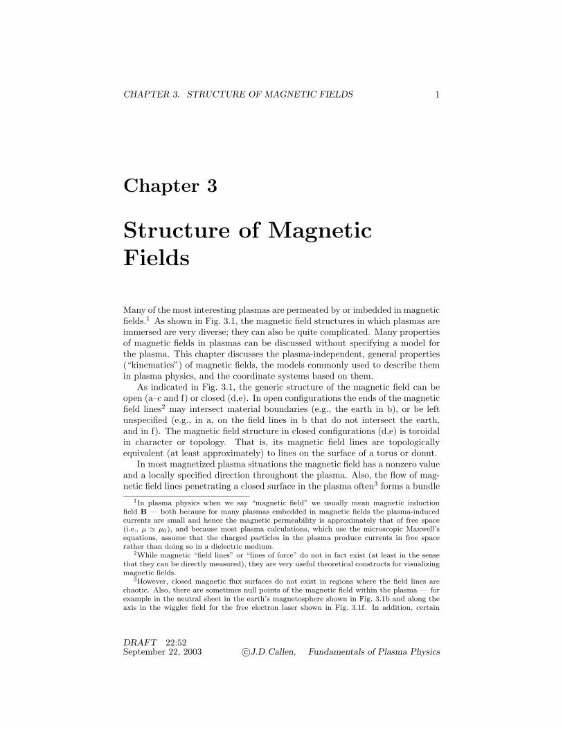
CHAPTER 3. STRUCTURE OF MAGNETIC FIELDS 1
Chapter 3
Structure of MagneticFields
Many of the most interesting plasmas are permeated by or imbedded in magneticfields.1 As shown in Fig. 3.1, the magnetic field structures in which plasmas areimmersed are very diverse; they can also be quite complicated. Many propertiesof magnetic fields in plasmas can be discussed without specifying a model forthe plasma. This chapter discusses the plasma-independent, general properties(“kinematics”) of magnetic fields, the models commonly used to describe themin plasma physics, and the coordinate systems based on them.
As indicated in Fig. 3.1, the generic structure of the magnetic field can beopen (a–c and f) or closed (d,e). In open configurations the ends of the magneticfield lines2 may intersect material boundaries (e.g., the earth in b), or be leftunspecified (e.g., in a, on the field lines in b that do not intersect the earth,and in f). The magnetic field structure in closed configurations (d,e) is toroidalin character or topology. That is, its magnetic field lines are topologicallyequivalent (at least approximately) to lines on the surface of a torus or donut.
In most magnetized plasma situations the magnetic field has a nonzero valueand a locally specified direction throughout the plasma. Also, the flow of mag-netic field lines penetrating a closed surface in the plasma often3 forms a bundle
1In plasma physics when we say “magnetic field” we usually mean magnetic inductionfield B — both because for many plasmas embedded in magnetic fields the plasma-inducedcurrents are small and hence the magnetic permeability is approximately that of free space(i.e., µ ! µ0), and because most plasma calculations, which use the microscopic Maxwell’sequations, assume that the charged particles in the plasma produce currents in free spacerather than doing so in a dielectric medium.
2While magnetic “field lines” or “lines of force” do not in fact exist (at least in the sensethat they can be directly measured), they are very useful theoretical constructs for visualizingmagnetic fields.
3However, closed magnetic flux surfaces do not exist in regions where the field lines arechaotic. Also, there are sometimes null points of the magnetic field within the plasma — forexample in the neutral sheet in the earth’s magnetosphere shown in Fig. 3.1b and along theaxis in the wiggler field for the free electron laser shown in Fig. 3.1f. In addition, certain
DRAFT 22:52September 22, 2003 c©J.D Callen, Fundamentals of Plasma Physics
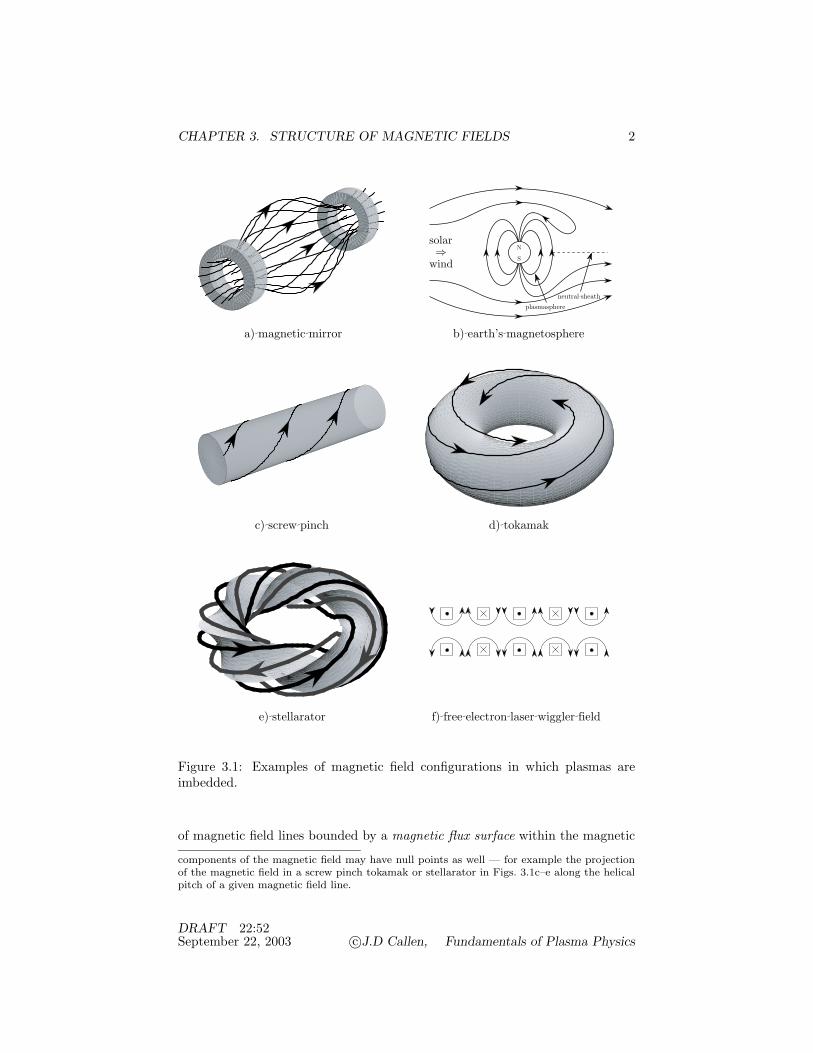
CHAPTER 3. STRUCTURE OF MAGNETIC FIELDS 2
plasmasphereneutral!sheath
N
S
solar⇒
wind
a)!magnetic!mirror b)!earth’s!magnetosphere
c)!screw!pinch d)!tokamak
e)!stellarator f)!free!electron!laser!wiggler!field
Figure 3.1: Examples of magnetic field configurations in which plasmas areimbedded.
of magnetic field lines bounded by a magnetic flux surface within the magnetic
components of the magnetic field may have null points as well — for example the projectionof the magnetic field in a screw pinch tokamak or stellarator in Figs. 3.1c–e along the helicalpitch of a given magnetic field line.
DRAFT 22:52September 22, 2003 c©J.D Callen, Fundamentals of Plasma Physics

CHAPTER 3. STRUCTURE OF MAGNETIC FIELDS 3
configuration. When nested magnetic flux surfaces exist, they usually providethe most natural magnetic-field-based coordinate system because most plasmaprocesses (charged particle motion, flows, transport) are much more rapid alongmagnetic field lines and within flux surfaces than across them.
The key magnetic field variations are evident in the magnetic field configura-tions illustrated in Fig. 3.1. Namely, while magnetic field lines point in a givendirection at any specified point, they can curve and twist, and their density canvary in space. The general properties of curves along a vector field such as themagnetic field are summarized in Section D.6.
The first section of this chapter introduces simple models (quadratic andsinusoidal magnetic well, and sheared slab magnetic field) that include the fourmost important local magnetic field properties for plasma physics (namely, par-allel and perpendicular gradients, curvature and shear). These simple modelswill be used to explore the most fundamental effects of magnetic fields in manyareas of plasma physics throughout the remainder of this book. The secondsection introduces the global magnetic field representations and magnetic-field-based coordinate systems that are used in modeling plasma processes on (longer)time scales where charged particles travel significant distances along magneticfields. While the magnetic fields in which plasmas are imbedded are seldomstraight in Cartesian coordinates, one can develop coordinate systems in whichthe magnetic field lines are straight. Such coordinates greatly facilitate analysesof magnetized plasmas. The third section develops the basic ideas of magneticisland structures that can form in the sheared slab model when a resonantperturbation is added. The next three sections discuss the simplest forms andproperties of magnetic field coordinate systems for open (Section 3.4) and closed(Sections 3.5, 3.6) magnetic field systems. Finally, Section 3.7 gives the generalforms of all the local differential propoerties of the vector magnetic field — gra-dients, divergence, curvature, shear and torsion, and the general expansion ofthe magnetic field B in terms of them.
3.1 Local Properties
The SI (mks) units for the magnetic field strength are webers/m2; thus, we canthink of the magnetic field strength as representing the number of magneticfield lines (webers) per unit area (m2). Typically, the magnetic field strengthvaries as we move along a magnetic field line. We can distinguish the effectsof variations in the magnetic field strength from the effects of changes in itsdirection by representing the magnetic field as
B = B(x) b, with b ≡ B/B, (3.1)
in which B ≡ |B| ≡ √B · B is the magnetic field strength and b is the local unit
vector along B, both at the point x. Since there are no magnetic monopoles innature, a magnetic field must be divergence free. (Such a vector field is calleda solenoidal field.) Thus, using the representation of B given in (3.1) and the
DRAFT 22:52September 22, 2003 c©J.D Callen, Fundamentals of Plasma Physics

CHAPTER 3. STRUCTURE OF MAGNETIC FIELDS 4
vector identity (??), we must have
0 = ∇· B = b ·∇B(!) + B ∇· b. (3.2)
An equation governing the variation of the magnetic field strength B along anyfield line can be determined by rearranging this equation to yield
∂B
∂!≡ b ·∇B = −B ∇· b, (3.3)
in which ! is the distance along a magnetic field line. Hence, if the magneticfield strength (number of field lines per unit area) is increasing (∂B/∂! > 0)as one moves along a magnetic field line, the local unit vectors along magneticfield lines must be converging (∇· b < 0); conversely, for a decreasing magneticfield strength (∂B/∂! < 0) the field line unit vectors diverge (∇· b > 0).
We will often be interested in describing mathematically the parallel (‖)variation of the magnetic field strength B. Near a minimum in the magneticfield strength along a magnetic field line the field strength B can be representedby a quadratic approximation:
Bqw = Bmin
(1 +
!2
L2‖
), quadratic well (qw) model, (3.4)
in which at B = Bmin where ! = 0 we have ∂B/∂!|!=0 = 0 and ∂2B/∂ !2|!=0 > 0,and by definition
L‖ ≡√
2 B
∂2B/∂!2
∣∣∣∣B=Bmin
. (3.5)
The characteristic scale length L‖ is the parallel distance over which the mag-netic field strength doubles — in this lowest order approximation.
The magnetic field strength often varies sinusoidally along a magnetic fieldline. A convenient model for this variation is
Bsin(!) = Bmin +(
Bmax − Bmin
2
)[1 − cos
(2π!L!
)]= Bmin +∆B sin2 π!
L!, sinusoidal (sin) model. (3.6)
Here, Bmax is the maximum field strength along a field line which occurs at! = ±L!/2 in this model, and ∆B ≡ Bmax − Bmin is the amplitude of thevariation of B along a field line within the periodicity length L!. The ! variationof Bsin near its minimum can be represented by the parabolic well model in(3.4) with L‖ = (Bmin/∆B)1/2L!/π. The ratio of the maximum to minimummagnetic field strength along a field line is:
Rm ≡ Bmax
Bmin= 1 +
∆B
Bmin, magnetic mirror ratio. (3.7)
DRAFT 22:52September 22, 2003 c©J.D Callen, Fundamentals of Plasma Physics

CHAPTER 3. STRUCTURE OF MAGNETIC FIELDS 5
Mirror ratios range from values of order 2 to 10 or more for typical magneticmirrors (Fig. 3.1a) and the earth’s magnetosphere (Fig. 3.1b), to only slightlygreater than unity in toroidal devices (Fig. 3.1d,e) where the magnetic fieldstrength varies only slightly as we move along the helical magnetic field linesfrom the outside to the inside of the torus. Note from (3.3) that at an extremum(minimum or maximum) of the magnetic field strength where ∂B/∂! = 0 thelocal unit vectors along field lines are divergence-free — they neither convergenor diverge.
The magnetic field can also vary — both in magnitude and direction —in directions perpendicular (transverse) to the magnetic field direction. Thesheared slab model, which we now discuss, approximates the local perpendicularvariations of typical magnetic field structures that are most important in plasmaphysics. In it a local Cartesian coordinate system is constructed at a given point.The z axis is taken to be along the magnetic field at the point where a magneticfield line passes through the origin of the coordinate system. The x axis istaken to be in the “radial” (across flux surface) direction in which the mostsignificant variations (in plasma parameters and in the density of magnetic fieldlines) occur in the plane perpendicular to the magnetic field. The y axis istaken to be in the azimuthal (or within flux surface) direction of least variation;i.e., it is the “ignorable” coordinate, at least approximately. For example, fora cylindrical magnetized plasma we anticipate mainly a radial variation in theplasma parameters: for this case the sheared slab model x, y, z coordinateswould correspond to r − r0, r0θ and z where r = r0 is the cylindrical radius ofthe magnetic field line that passes through the origin of the sheared slab model.The word slab in the title of the model indicates that only a thin “radial” (x)slice of the magnetic configuration is being considered.
A local expansion of the magnetic field that captures its most importantperpendicular variations is
Bss = B0
[(1 +
x
LB
)ez +
z
RCex +
x
LSey
], sheared slab (ss) model,
(3.8)
in which B0 is the strength of the magnetic field (or density of magnetic fieldlines) at the origin where x ≡ (x, y, z) = (0, 0, 0). Here, as indicated in Fig. 3.2,the ez term represents the lowest order magnetic field (the unity) and the per-pendicular spatial gradient of its magnitude (1/LB), the ex term represents themagnetic field curvature (1/RC), and the ey term represents the differentialtwisting (shear, 1/LS) of the magnetic field lines. These fundamental magneticfield properties will be explained and defined more precisely below and in thefollowing sections. [Torsion (uniform twisting — see Section 3.7 below and D.6)of magnetic field lines such as in a uniform helical twist of the field lines in thescrew pinch shown in Fig. 3.1c is not included in the sheared slab model becausethe ez vector is taken to be in a locally fixed rather than rotating direction.]Since the model represents a Taylor series expansion of the magnetic field abouta given point, it is only valid for small distances from the origin — |x/LB | << 1,
DRAFT 22:52September 22, 2003 c©J.D Callen, Fundamentals of Plasma Physics

CHAPTER 3. STRUCTURE OF MAGNETIC FIELDS 6
x
x
x
y
y
y
z
z
zB
B
B
x0
x0
x0
x(!)
y(!,!x)
d!
d!
∥
∥
∥ Rc
Ls
∥
∇B0
Figure 3.2: Magnetic field line characteristics included in the sheared slab mag-netic field model. Each sketch indicates the behavior of magnetic field lineswhen only the indicated coefficient does not vanish.
|z/RC | << 1, |x/LS | << 1.Calculating the magnitude of the magnetic field using B ≡ |B| =
√B · B,
we find, to lowest order in the distance from the origin,
Bss ≡ |Bss| = B0
(1 +
x
LB+ O
x2
L2B
,x2
L2S
,z2
R2C
)& B0
(1 +
x
LB
). (3.9)
DRAFT 22:52September 22, 2003 c©J.D Callen, Fundamentals of Plasma Physics
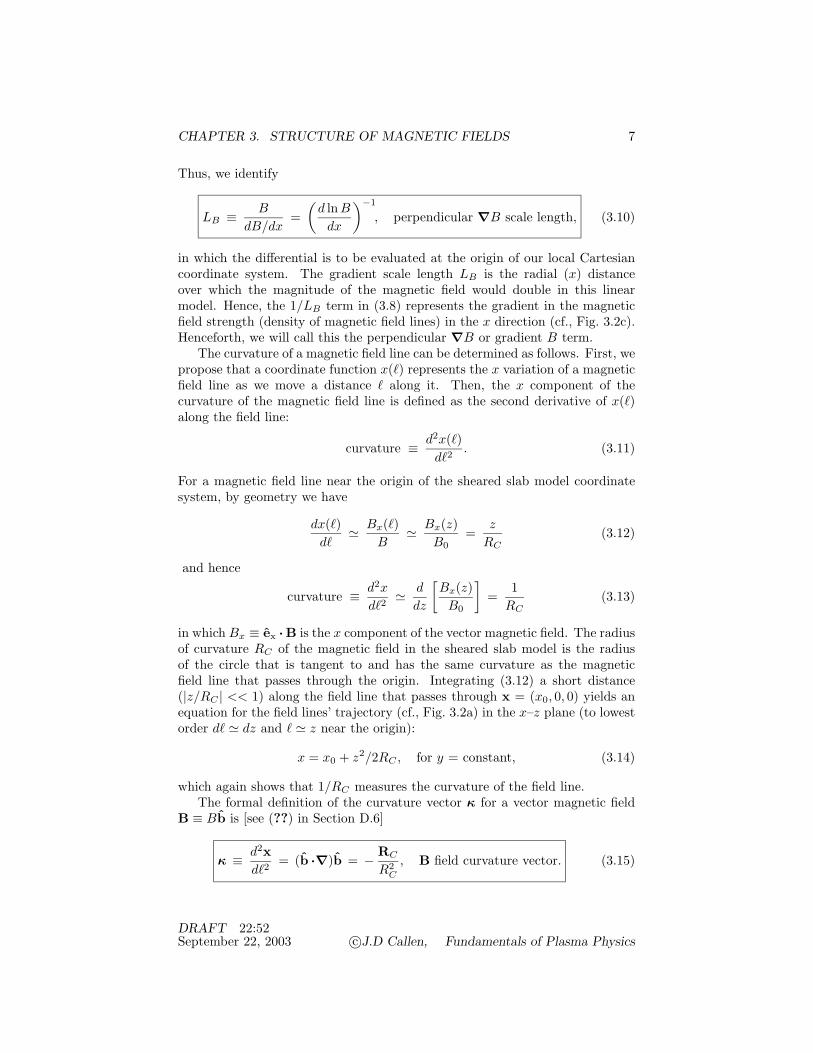
CHAPTER 3. STRUCTURE OF MAGNETIC FIELDS 7
Thus, we identify
LB ≡ B
dB/dx=
(d lnB
dx
)−1
, perpendicular ∇B scale length, (3.10)
in which the differential is to be evaluated at the origin of our local Cartesiancoordinate system. The gradient scale length LB is the radial (x) distanceover which the magnitude of the magnetic field would double in this linearmodel. Hence, the 1/LB term in (3.8) represents the gradient in the magneticfield strength (density of magnetic field lines) in the x direction (cf., Fig. 3.2c).Henceforth, we will call this the perpendicular ∇B or gradient B term.
The curvature of a magnetic field line can be determined as follows. First, wepropose that a coordinate function x(!) represents the x variation of a magneticfield line as we move a distance ! along it. Then, the x component of thecurvature of the magnetic field line is defined as the second derivative of x(!)along the field line:
curvature ≡ d2x(!)d!2
. (3.11)
For a magnetic field line near the origin of the sheared slab model coordinatesystem, by geometry we have
dx(!)d!
& Bx(!)B
& Bx(z)B0
=z
RC(3.12)
and hence
curvature ≡ d2x
d!2& d
dz
[Bx(z)
B0
]=
1RC
(3.13)
in which Bx ≡ ex · B is the x component of the vector magnetic field. The radiusof curvature RC of the magnetic field in the sheared slab model is the radiusof the circle that is tangent to and has the same curvature as the magneticfield line that passes through the origin. Integrating (3.12) a short distance(|z/RC | << 1) along the field line that passes through x = (x0, 0, 0) yields anequation for the field lines’ trajectory (cf., Fig. 3.2a) in the x–z plane (to lowestorder d! & dz and ! & z near the origin):
x = x0 + z2/2RC , for y = constant, (3.14)
which again shows that 1/RC measures the curvature of the field line.The formal definition of the curvature vector κ for a vector magnetic field
B ≡ Bb is [see (??) in Section D.6]
κ ≡ d2xd!2
= (b ·∇)b = − RC
R2C
, B field curvature vector. (3.15)
DRAFT 22:52September 22, 2003 c©J.D Callen, Fundamentals of Plasma Physics

CHAPTER 3. STRUCTURE OF MAGNETIC FIELDS 8
Evaluating this expression for the sheared slab model magnetic field in (3.8),we obtain (near the origin where d! & dz and |x| << LB)
κ =∂b∂!
& ∂
∂z
[ez +
(z/RC) ex + (x/LS) ey
1 + x/LB
]& 1
RCex ≡ κxex. (3.16)
Thus, RC is the inverse of the (normal, x direction) curvature of the magneticfield:
RC ≡ 1/|κx|, radius of curvature. (3.17)
Note that the absolute value is needed because vectorially the radius of curvaturevector RC points in the opposite direction from the curvature vector: κ =−RC/R2
c — see Fig. ?? and Eq. (??) in Section D.6. Thus, for the shearedslab model the vectorial radius of curvature is RC ≡ −κ/|κ|2 = −RC ex, whichpoints from the point x = (RC , 0, 0) to the origin.
The magnetic field line curvature vector κ can in general be written in a moreillustrative and useful form (for situations where currents flow in the plasma)using b ≡ B/B and the magnetostatic Ampere’s law ∇×B = µ0J:
κ ≡ (b ·∇)b = − b×(∇×b) = − b×(∇×B/B)= − b×[∇(1/B)×B] − b×(∇×B)/B = − b×(b×∇ lnB) + µ0J×B/B2
= (1/B)[∇ − b(b ·∇)]B + µ0J×B/B2, (3.18)
in which the vector identities (??), (??), and (??) have been used in successivesteps. Defining
∇⊥ ≡ ∇ − b (b ·∇) = − b×(b×∇), gradient perpendicular to B, (3.19)
to represent the components of the gradient operator in directions perpendicularto the magnetic field B, we can write the final form in (3.18) in general as
κ = ∇⊥ lnB +µ0J×B
B2, relation of curvature to ∇⊥B and J. (3.20)
Near the origin of the sheared slab model, the ex component of this equationyields
κx ≡ 1RC
=1B
dB
dx+
µ0Jy
B=
1LB
+µ0Jy
B. (3.21)
When there is no current in the ey direction in the sheared slab model, we have1/RC = 1/LB .
The shear in a magnetic field can be understood as follows. A magnetic fieldline can rotate about the z axis because of torsion (twisting at a constant angularrate) and shear (differential twisting) — see Section D.6. As noted above, thesheared slab model does not include torsion. The shear in the magnetic field
DRAFT 22:52September 22, 2003 c©J.D Callen, Fundamentals of Plasma Physics

CHAPTER 3. STRUCTURE OF MAGNETIC FIELDS 9
can be defined for our Cartesian coordinate system through the x derivative ofthe y(!) coordinate variation along a magnetic field line:
shear ≡ d
dx
[dy(!)d!
]. (3.22)
For a magnetic field line near the origin of the sheared slab model coordinatesystem, by geometry we have
dy(!)d!
& By
B0& x
LS.
Thus, in the sheared slab model we have
shear ≡ d
dx
(dy
d!
)& d
dx
[By(x)
B0
]& 1
LS. (3.23)
The shear length LS is the linear extrapolation distance in the x direction overwhich the magnetic field would differentially twist through an angle of one radian(i.e., to where By = B0). Integrating (3.22) a short distance (|z/LS | << 1) alongthe field line that passes through the point x = (x, y0, 0) yields an equation forits trajectory (cf., Fig. 3.2b) in the y–z plane:
y = y0 + x z/LS , for x = constant, (3.24)
which shows that 1/LS measures the differential twisting of the field lines outof the the x–z plane and hence the shear in the magnetic field lines.
The formal definition of the local shear ς in a vector field B ≡ Bb is [see(3.151) below and (??) in Section D.6]
ς ≡ (b×∇ψ) · ∇×(b×∇ψ)|b×∇ψ|2 =
(B×∇ψ) · ∇×(B×∇ψ)B2|∇ψ|2 , local shear
(3.25)
in which ∇ψ is the gradient of an assumed magnetic flux function ψ and forthe last form we have used (3.1) and vector identities (??), (??) and (??). Forour sheared slab model ψ → x, ∇ψ → ∇x = ex and thus b×∇ψ → b×ex =ey − ez(x/LS)/(1 +x/LB). Note that near the origin of the sheared slab modelgeometry |b| & 1 and |b×∇ψ| & 1. Thus, evaluating the shear definition in(3.25) for the sheared slab model we obtain
ς & ey · ∇×(b×ex) & 1/LS . (3.26)
By construction, the magnetic field in the sheared slab model satisfies thesolenoidal or no magnetic monopole condition for a magnetic induction field,i.e., ∇· Bss = 0. However, its curl (rotation) does not vanish:
∇×Bss = B0
[(1
RC− 1
LB
)ey +
1LS
ez
]. (3.27)
DRAFT 22:52September 22, 2003 c©J.D Callen, Fundamentals of Plasma Physics

CHAPTER 3. STRUCTURE OF MAGNETIC FIELDS 10
In equilibrium situations where the magnetostatic Ampere’s law ∇×B = µ0Japplies, the full generality of the sheared slab model is appropriate only if elec-trical currents flow in the plasma. For vacuum or very low plasma pressuresituations where no significant currents flow in a magnetized plasma, we musthave 1/RC = 1/LB and 1/LS = 0. The curvature (1/RC) can deviate from theinverse gradient length (1/LB) only if electrical current flows in the y direction,as indicated by both (3.21) and (3.27). Since for strong magnetic fields it isharder for charged particles and hence plasma currents to flow across magneticfields compared to along them, the y component of the current is typically smalland usually 1/RC & 1/LB . Magnetic shear (1/LS) is possible (in this torsion-free model) only if current flows in the z (magnetic field) direction. These pointswill be made more quantitatively explicit in Sections 3.7, 5.3 and 20.1.
The parallel quadratic well, sinusoidal and sheared slab models represent themost important spatial variations of the magnetic field around a given point.Any given physical situation can be modeled with these models by specifyingthe characteristic scale lengths for the local properties of the magnetic field:parallel gradient B scale lengths L‖ and L!, perpendicular gradient B length LB ,curvature radius RC and shear length LS . While these models provide suitablelowest order “local” descriptions for most magnetized plasma situations, theyare not the most general magnetic field descriptions. In particular, they do notallow for torsion or all the possible magnetic field variations in the y and zdirections. The most general local expansion of a magnetic field is discussed inSection 3.7. Also, the local expansions do not in general provide global (i.e., validover all space) descriptions of the magnetic field. The remaining sections of thischapter develop more complete, but correspondingly more complex, magneticfield models.
3.2 Magnetic Field Representations and Coor-dinate Systems
In the preceding section we developed local Taylor series expansions of a mag-netic field B about a given point. While these expansions are very useful forunderstanding the local differential properties (gradients, curvature, shear) of amagnetic field, in general they do not provide a global description of it. Chargedparticles in plasmas move over long distances along magnetic field lines for mosttime scales of interest. Also, they typically move much more rapidly along mag-netic field lines than perpendicular to them; this causes the properties of amagnetized plasma to be very anisotropic relative to the magnetic field direc-tion. In order to develop compact descriptions of magnetized plasmas it is mostconvenient to use coordinate systems based on the global structure of the mag-netic field — so-called magnetic field line or magnetic flux coordinate systems.Magnetic flux coordinates are curvilinear coordinates that are chosen so thatthe equation of a magnetic field line is a straight line in the chosen coordi-nates. They are the most useful coordinates because they facilitate separation
DRAFT 22:52September 22, 2003 c©J.D Callen, Fundamentals of Plasma Physics

CHAPTER 3. STRUCTURE OF MAGNETIC FIELDS 11
of plasma effects along and perpendicular to magnetic field lines. This sectiondiscusses calculations of magnetic field lines, and magnetic field representationsand coordinate systems that describe the entire magnetic field structure.
The global structure of the magnetic field can in principle be obtained bysimply integrating the differential equations of a curve that follows a magneticfield line. Defining x(!) to be the trajectory along a magnetic field line, thevector dx(!)/d! that is locally tangent to the magnetic field is given by
dx(!)d!
∣∣∣∣along B
=BB
= b, field line equation. (3.28)
This is the fundamental definition of a magnetic field line that we will usethroughout the remainder of this book. Taking the ex, ey, and ez projectionsof this fundamental field line definition, we obtain
dx
Bx=
dy
By=
dz
Bz=
d!
B. (3.29)
Note that these field line differential equations can also be obtained from thecondition that a vector differential length d" along the magnetic field B mustbe parallel to it: d"×B = 0.
For simple magnetic field systems we can directly integrate the three inde-pendent equations in (3.29) to obtain a mathematical description of the mag-netic field. For example, we performed such integrations for the sheared slabmodel in the special cases of no shear and little perpendicular gradient B orcurvature — see (3.14) and (3.24). For such systems the constants of integra-tion provide labels for the magnetic field lines — x0 and y0 for the two specialsheared slab model cases. However, it is often impractical or impossible toobtain a global magnetic field description by directly integrating the equationsthat describe a magnetic field line trajectory. For example, integrating the threeequations for the complete sheared slab model in (3.8) results in a set of threeinterrelated, implicit equations for which a closed solution is not possible, exceptin the vicinity of the origin (see Problem 3.7).
For a magnetic field in free space (i.e., in a vacuum), or in the limit wherethe currents flowing in the plasma are negligible, the equilibrium Ampere’s lawbecomes simply ∇×B = 0. This equation can be satisfied by writing themagnetic field in terms of a scalar potential ΦM :
B = −∇ΦM , vacuum magnetic field representation. (3.30)
For this case the solenoidal (no magnetic monopoles) condition ∇· B = 0 be-comes the Laplace equation
∇2ΦM = 0. (3.31)
Methods for solving the Laplace equation in various geometries are available inmany books on electromagnetic theory and other areas of physics. For magne-tized plasmas such solutions are useful mainly in vacuum regions outside the
DRAFT 22:52September 22, 2003 c©J.D Callen, Fundamentals of Plasma Physics

CHAPTER 3. STRUCTURE OF MAGNETIC FIELDS 12
plasma, or as the lowest order magnetic field structure for cases where currentsin the plasma do not significantly change the magnetic field. However, for manyimportant magnetized plasma situations the electrical currents flowing in theplasma are significant, and in fact very important, in determining the structureand even topology of the magnetic field. Thus, solutions of (3.31) for vacuummagnetic fields are not always useful for magnetized plasmas and we must lookelsewhere for broadly applicable descriptions.
Like any vector field subject to the solenoidal condition (∇· B = 0), themagnetic induction field B can be written in terms of a vector potential A:
B = ∇×A. (3.32)
For example, an appropriate vector potential for the sheared slab model is
Ass = B0
(x +
x2
2LB− z2
2RC
)ey − B0
x2
2LSez, (3.33)
as can be verified by substituting it into (3.32) and comparing the result to(3.8).
Alternatively (see Section D.5), the magnetic field can be written as
B = ∇α×∇β, Clebsch representation, (3.34)
in which α(x) and β(x) are scalar stream functions (i.e., functions that areconstant along the vector field B) since B ·∇α = B ·∇β = 0. Note that therepresentations of B in (3.32) and (3.34) are equivalent if we define
A = α∇β, or A = −β∇α, (3.35)
since using vector identities (??), (??), and (??), we have ∇×α∇β = ∇α×∇βand −∇×β∇α= −∇β×∇α= ∇α×∇β. Note also that the vector potential Aand the stream functions α,β are somewhat arbitrary since they yield the samemagnetic induction field B under the gauge transformations A → A + ∇χ(x),and α → α + f1(β) or β → β + f2(α) (but not both f1, f2 simultaneously) inwhich χ, f1, and f2 are arbitrary scalar functions of the variables indicated.While the stream functions α,β must be continuous, they can be multivalued(e.g., they can involve angular or cyclic variables). For examples of α and βstream functions, see Problem 3.7, which develops them for the sheared slabmodel, and the following sections.
The Clebsch representation of the magnetic field can be used as a basis fora coordinate system that represents the global magnetic field structure — theClebsch magnetic coordinate system. Along magnetic field lines, which followthe curve given by (3.28), we have dα/d! = (dx/d!) ·∇α = (B ·∇α)/B = 0and similarly dβ/d! = 0. Thus, magnetic field lines lie within α(x) = constantand β(x) = constant surfaces. Further, since ∇α×∇β points in the direction of(and is equal to) B, the intersection of the α,β surfaces defines a given magneticfield line. Hence, α and β are labels for a particular magnetic field line.
DRAFT 22:52September 22, 2003 c©J.D Callen, Fundamentals of Plasma Physics
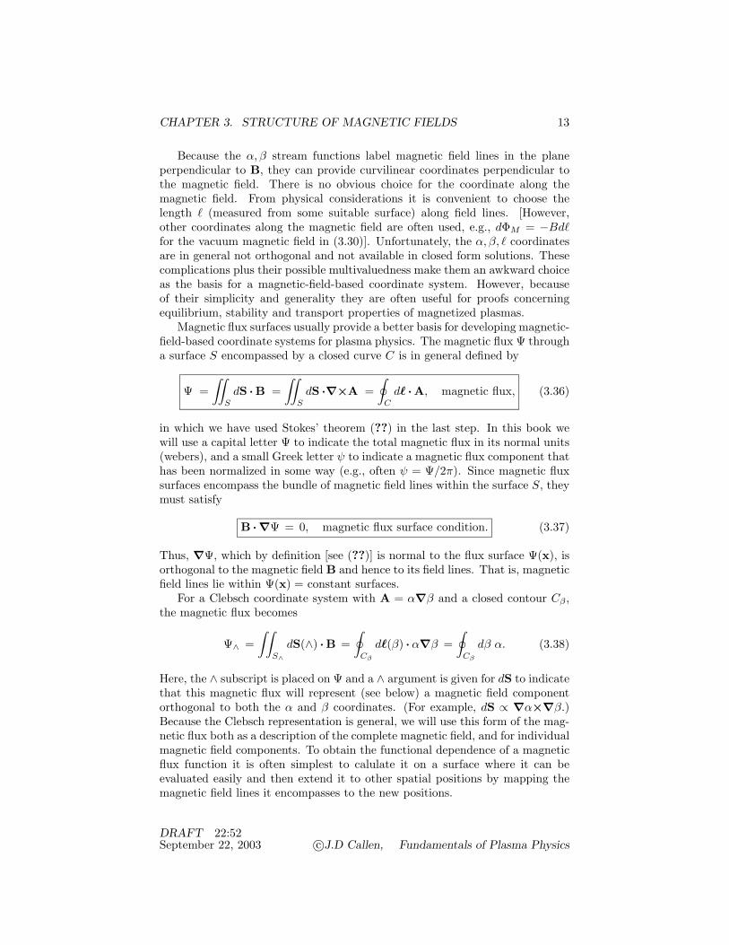
CHAPTER 3. STRUCTURE OF MAGNETIC FIELDS 13
Because the α,β stream functions label magnetic field lines in the planeperpendicular to B, they can provide curvilinear coordinates perpendicular tothe magnetic field. There is no obvious choice for the coordinate along themagnetic field. From physical considerations it is convenient to choose thelength ! (measured from some suitable surface) along field lines. [However,other coordinates along the magnetic field are often used, e.g., dΦM = −Bd!for the vacuum magnetic field in (3.30)]. Unfortunately, the α,β, ! coordinatesare in general not orthogonal and not available in closed form solutions. Thesecomplications plus their possible multivaluedness make them an awkward choiceas the basis for a magnetic-field-based coordinate system. However, becauseof their simplicity and generality they are often useful for proofs concerningequilibrium, stability and transport properties of magnetized plasmas.
Magnetic flux surfaces usually provide a better basis for developing magnetic-field-based coordinate systems for plasma physics. The magnetic flux Ψ througha surface S encompassed by a closed curve C is in general defined by
Ψ =∫∫
SdS · B =
∫∫S
dS ·∇×A =∮
Cd" · A, magnetic flux, (3.36)
in which we have used Stokes’ theorem (??) in the last step. In this book wewill use a capital letter Ψ to indicate the total magnetic flux in its normal units(webers), and a small Greek letter ψ to indicate a magnetic flux component thathas been normalized in some way (e.g., often ψ = Ψ/2π). Since magnetic fluxsurfaces encompass the bundle of magnetic field lines within the surface S, theymust satisfy
B · ∇Ψ = 0, magnetic flux surface condition. (3.37)
Thus, ∇Ψ, which by definition [see (??)] is normal to the flux surface Ψ(x), isorthogonal to the magnetic field B and hence to its field lines. That is, magneticfield lines lie within Ψ(x) = constant surfaces.
For a Clebsch coordinate system with A = α∇β and a closed contour Cβ ,the magnetic flux becomes
Ψ∧ =∫∫
S∧dS(∧) · B =
∮Cβ
d"(β) · α∇β =∮
Cβ
dβ α. (3.38)
Here, the ∧ subscript is placed on Ψ and a ∧ argument is given for dS to indicatethat this magnetic flux will represent (see below) a magnetic field componentorthogonal to both the α and β coordinates. (For example, dS ∝ ∇α×∇β.)Because the Clebsch representation is general, we will use this form of the mag-netic flux both as a description of the complete magnetic field, and for individualmagnetic field components. To obtain the functional dependence of a magneticflux function it is often simplest to calulate it on a surface where it can beevaluated easily and then extend it to other spatial positions by mapping themagnetic field lines it encompasses to the new positions.
DRAFT 22:52September 22, 2003 c©J.D Callen, Fundamentals of Plasma Physics

CHAPTER 3. STRUCTURE OF MAGNETIC FIELDS 14
Magnetic flux surfaces can be constructed easily for magnetic configurationsor magnetic field components in which there is symmetry (i.e., no dependenceon a coordinate) in a direction perpendicular to the magnetic field. Then,we choose β to be that symmetry coordinate, and the magnetic flux and thecorresponding vector potential become
Ψ∧ = α∮
dβ, Aβ = α∇β =Ψ∧∮dβ
∇β, for symmetry in β. (3.39)
When there is symmetry in the β direction, the magnetic field component pro-duced by the component of the vector potential in the ∇β direction can berepresented in terms of the corresponding magnetic flux by
B∧ = ∇×Aβ = ∇(Ψ∧∮dβ
)×∇β, for symmetry in β. (3.40)
This component of the magnetic field is labeled with a vector cross productsubscript (∧) because it is orthogonal to both the symmetry coordinate and theflux coordinate directions: B∧ · ∇β = 0, and B∧ · ∇Ψ∧ = 0. Note that Ψ∧ isclearly a magnetic flux function since it satisfies (3.37). As a simple example ofhow to directly use these formulas for a single component magnetic field, Section3.4 develops the magnetic flux (and Clebsch) coordinates for an axisymmetricmagnetic mirror.
These formulas can be used to develop magnetic flux coordinates for thesheared slab model as follows. In the absence of magnetic shear (i.e., for 1/LS →0), the sheared slab model is symmetric in the y direction. For this case, thedominant or “main” magnetic field component in the sheared slab model canbe calculated by taking β = y,
∮dβ = y0. Then, we use the rectangular
surface in the z = 0 plane specified by (see Fig. 3.3a) 0 ≤ x ≤ x0 and 0 ≤y ≤ y0 for calculating the magnetic flux in the z direction to yield Ψz|z=0 =∫ x0
0 dx∫ y0
0 dy Bz = (x0 +x20/2LB)y0B0 at z = 0. This magnetic flux is extended
to other (small) z values using the field line label x0 = x− z2/2RC from (3.14)to yield:
Ψz &(
x +x2
2LB− z2
2RC
)y0B0 & x y0B0, Ay ≡ Ψy
y0∇y,
Bmain = ∇×Ay = ∇(Ψz
y0
)× ey & B0
[(1 +
x
LB
)ez +
z
RCex
]. (3.41)
To determine a similar magnetic flux form for the “auxiliary” magnetic shearcomponent in the sheared slab model, we consider the case where the perpen-dicular gradient in B and curvature are absent (i.e., 1/LB = 0 and 1/RC = 0),and the field line label simplifies to x0 = x. Then, there is symmetry in thez direction, and we take β = z,
∮dβ = z0. Using the rectangular surface in
the y = 0 plane specified by (see Fig. 3.3b) 0 ≤ x ≤ x0 and 0 ≤ z ≤ z0, weobtain Ψy|y=0 = − ∫ x0
0 dx∫ z0
0 dz By = − (x20/2LS)z0B0. (The Ψy magnetic flux
DRAFT 22:52September 22, 2003 c©J.D Callen, Fundamentals of Plasma Physics

CHAPTER 3. STRUCTURE OF MAGNETIC FIELDS 15
x
x
yy
zz
By(x)B
x0
y0
z0
x0
a)!!main!magnetic!flux!ym b)!!auxiliary!magnetic!flux!y*
Figure 3.3: Geometry of the surfaces through which the (a) main (Ψz) and (b)auxiliary (Ψy) magnetic fluxes are calculated for the sheared slab magnetic fieldmodel.
is negative because dS ≡ d"x×d"z = exdx×ezdz = −eydxdz.) Using x0 = x,this yields
Ψy = − x2
2LSz0B0, Az ≡ Ψy
z0∇z,
Baux = ∇×Az = ∇(Ψy
z0
)× ez = B0
x
LSey. (3.42)
The total magnetic field in the sheared slab model can be represented interms of its y and z magnetic flux components by adding these two results:
Bss = Bmain + Baux = ∇(Ψz/y0)×∇y + ∇(Ψy/z0)×∇z. (3.43)
Neglecting terms of order x2 and z2, the two components in (3.43) can becombined into a single form B & ∇B0(x+x2/2LB−z2/2RC)×∇(y−x z/LS) =∇Ψz×∇y0 using (3.24), which is in the Clebsch form given in (3.34). However,in general the two magnetic flux forms cannot be combined into a single Clebschform. For the sheared slab model the natural curvilinear coordinates near theorigin that can be deduced from this magnetic flux model of the magnetic fieldare Ψz, y0 ≡ y − x z/LS and ! & z. Note that despite the presence of magneticshear, curvature and a perpendicular gradient of B, magnetic field lines are, asdesired, straight to first order in this magnetic flux coordinate system: dΨz/d! =0, dy0/d! = 0, and d! & dz along field lines.
Many physically relevant situations are more complicated, either becausethey are fully three-dimensional and have no symmetry direction (e.g., the outerparts of the earth’s magnetosphere in Fig. 3.1b and the stellarator in Fig. 3.1e),or because there is a magnetic field component in the symmetry direction(s)
DRAFT 22:52September 22, 2003 c©J.D Callen, Fundamentals of Plasma Physics

CHAPTER 3. STRUCTURE OF MAGNETIC FIELDS 16
(e.g., the screw pinch in Fig. 3.1e and the tokamak in Fig. 3.1d). When thereis more than one magnetic field component and one of the components is in asymmetry direction, the magnetic induction field B can be written in terms ofthe magnetic flux components associated with a main (parallel to a symmetryor periodicity direction) and an auxiliary (perpendicular to the dominant sym-metry direction, or due to shear, torsion) component of the magnetic field. Eachmagnetic field component can be written in terms of the relevant magnetic fluxin a Clebsch form using (3.40).
In general, representations of B fields can always be constructed with twomagnetic flux functions. They are quite useful in plasma physics. A single ortotal Clebsch form can be developed from them whenever the two flux functionsare single valued functions of each other, which happens when they representconfigurations with closed, nested toroidal magnetic flux surfaces. Examples ofsuch systems include axisymmetric toroidal configurations (see Section 3.6) andsome regions of stellarators.
For toroidal magnetic configurations with helical magnetic field lines thereare two natural cyclic coordinates: the toroidal (long way around the torus) andpoloidal (short way) angles ζ and θ. For the moment these will be arbitrarily-defined angles; they are only required to span their respective spaces. Then, inanalogy with (3.41) and (3.42), it can be shown in general that the magneticfield can be written in the form of toroidal (tor) and poloidal (pol) magneticfield and flux components:
B = Btor + Bpol = ∇(Ψtor/2π)×∇θ + ∇ζ×∇(Ψpol/2π). (3.44)
The natural sign of the poloidal magnetic flux Ψpol would be negative for thisgeometry because of the choice of Ψ, θ, ζ as a right-handed set of coordinates;however, by convention its sign is changed in this definition. The magnetic axis(origin) for the poloidal angle coordinate θ is defined to be the line on whichBpol ≡ ∇ζ×∇(Ψpol/2π) vanishes.
In regions where a set of nested toroidal magnetic flux surfaces exist, thepoloidal flux function is a single-valued (monotonic) function of the toroidalflux function and hence can be written in terms of it: Ψpol = Ψpol(Ψtor). Then,the poloidal and toroidal angles can be modified (θ → θf and ζ → ζf), so thatmagnetic field lines are “straight” in them (hence, the f subscript indicatingproper flux surface coordinates). (See Section 3.6 for the development of suchstraight-field-line coordinates for axisymmetric toroidal configurations.) Thus,for toroidal configurations with nested flux surfaces, the magnetic field in (3.44)can be written compactly in the Clebsch form
B = ∇(Ψtor
2π
)×∇
[θf −
( ι2π
)ζf
], toroidal flux surfaces B field,
(3.45)
DRAFT 22:52September 22, 2003 c©J.D Callen, Fundamentals of Plasma Physics

CHAPTER 3. STRUCTURE OF MAGNETIC FIELDS 17
where we have defined
ι(Ψtor) ≡ 2π(
dΨpol
dΨtor
), rotational transform angle (degrees), (3.46)
which is the slope (dθf/dζf) of the magnetic field lines in the θf–ζf plane. Here,ι is the small Greek letter iota; it is divided by 2π in many formulas to representthe angle of field line rotation (per toroidal transit) in radians. For this modelmagnetic field we identify the Clebsch coordinates as α = Ψtor/2π and β =θf−(ι/2π) ζf . Along magnetic field lines we have dα = dΨtor/2π = 0 and dβ = 0or dθf = (ι/2π) dζf =⇒ θf = (ι/2π) ζf + constant. Thus, magnetic field lines arestraight in the Ψtor =constant, θf– ζf plane. For such toroidal configurations thenatural magnetic field curvilinear coordinates are those based on the magneticflux coordinates Ψtor, θf , and ζf , which unfortunately are not usually orthogonal.Nonetheless, since ι/2π is typically not a rational number (ratio of integers,see Section 3.6), the magnetic flux coordinates usually provide a more usefuldescription than the Clebsch coordinates — because of the multivaluedness ofthe β coordinate in θf and ζf and because ! (or some other coordinate along fieldlines) is not one of the natural coordinates of the magnetic field description.
3.3 Magnetic Islands
This section will explain how an error magnetic field can create a magnetic islandin a sheared magnetic field model — it is yet to be written and inserted. Themain point of this section will be to show that when a resonant magnetic fieldperturbation of the type Bx = −Bx sin ky is added to the sheared slab modelit produces a magnetic island of width w = 4 (LSBx/kB0)1/2 and to elucidatevarious properties of field lines in and around the magnetic island structure.
3.4 Open Magnetic Configurations*
There are many types of open magnetic configurations: a cylindrical columnof magnetized plasma, magnetic mirrors (Fig. 3.1a), the earth’s magnetosphere(Fig. 3.1b), the interplanetary magnetic field, solar flares, cusps (produced bypairs of mirror coils in which the coil currents flow in opposite directions),and so-called divertor regions on open field lines that are outside the closedflux surfaces in toroidal configurations. The simplest and conceptually mostimportant open configurations are of the axisymmetric magnetic mirror type,as shown in Fig. 3.4.
We consider first an axisymmetric magnetic mirror composed of two identicalcurrent-carrying solenoidal coils separated by a distance L, as shown in Fig. 3.4a.This “simple mirror” is an important paradigm for discussing many effects ofgeometry on magnetized plasmas. Since there is symmetry in the azimuthal (θ)
DRAFT 22:52September 22, 2003 c©J.D Callen, Fundamentals of Plasma Physics
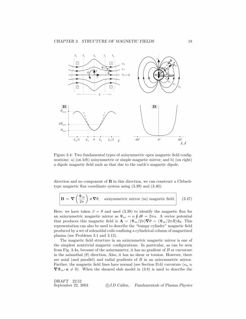
CHAPTER 3. STRUCTURE OF MAGNETIC FIELDS 18
∥
!0 !1 !2-!2 -!1
ψ0!=!0
ψ1
ψ2
L
∇ψ ∇!
M
z
S
Nϑ
ϕ
r0ψ0
ψ1ψ2
r
B
∇ψ
|B|
-60° 60°0°
|B|Bmax
Bmin
2Bmin
-L!/2 -L‖ L‖ L!/20 !
BR
Z
Figure 3.4: Two fundamental types of axisymmetric open magnetic field config-urations: a) (on left) axisymmetric or simple magnetic mirror; and b) (on right)a dipole magnetic field such as that due to the earth’s magnetic dipole.
direction and no component of B in this direction, we can construct a Clebsch-type magnetic flux coordinate system using (3.39) and (3.40):
B = ∇(Ψm
2π
)×∇θ, axisymmetric mirror (m) magnetic field. (3.47)
Here, we have taken β = θ and used (3.39) to identify the magnetic flux foran axisymmetric magnetic mirror as Ψm = α
∮dθ = 2πα. A vector potential
that produces this magnetic field is A = (Ψm/2π)∇θ = (Ψm/2πR) eθ. Thisrepresentation can also be used to describe the “bumpy cylinder” magnetic fieldproduced by a set of solenoidal coils confining a cylindrical column of magnetizedplasma (see Problems 3.1 and 3.12).
The magnetic field structure in an axisymmetric magnetic mirror is one ofthe simplest nontrivial magnetic configurations. In particular, as can be seenfrom Fig. 3.4a, because of the axisymmetry, it has no gradient of B or curvaturein the azimuthal (θ) direction, Also, it has no shear or torsion. However, thereare axial (and parallel) and radial gradients of B in an axisymmetric mirror.Further, the magnetic field lines have normal (see Section D.6) curvature (κN ∝∇Ψm· κ -= 0). When the sheared slab model in (3.8) is used to describe the
DRAFT 22:52September 22, 2003 c©J.D Callen, Fundamentals of Plasma Physics

CHAPTER 3. STRUCTURE OF MAGNETIC FIELDS 19
local magnetic field in a simple mirror, we make the following associations:(x, y, z) → (Ψm, θ, !), 1/RC = κx → ∇Ψm · κ/|∇Ψm|, 1/LB = (1/B)(dB/dx)→ |∇Ψm|(1/B)(∂B/∂Ψm), 1/LS → 0.
In a simple mirror the magnetic field strength varies significantly along mag-netic field lines. It is smallest at the midplane (Z = 0) between the mirrors andmaximum in the mirror “throats” (Z = ±L/2) of the two coils. Since the vari-ation of |B| along magnetic field lines is approximately sinusoidal between themirror coils, it is commonly represented by the sinusoidal model in (3.6). Nearthe midplane at ! = Z = 0, to lowest order the variation of the magnetic fieldstrength is quadratic in ! and can be represented by the quadratic well model(3.4). The mirror ratio Rm ≡ Bmax/Bmin increases with minor radius R fromits minimum on the axis of symmetry (R = 0). When the mirror coils areseparated by approximately their diameters, its on-axis value is about 2–3.
The magnetic flux coordinate system Ψm, θ, ! for a simple mirror can berelated to a cylindrical coordinate system R, θ, Z constructed about the sym-metry axis of the magnetic mirror. For simplicity we define ! = 0, Z = 0 at themidplane between the two mirror coils. We calculate the relation between thedistance ! along a field line and the axial cylindrical coordinate Z as follows.First, we take the dot product of the field line equation (3.28) with eZ ≡ ∇Zto obtain
dZ
d!=
BZ
B. (3.48)
Since there is no azimuthal magnetic field component (Bθ ≡ eθ · B = 0) andnear the axis of symmetry (R = 0) we can see from Fig. 3.4a that BR << BZ ,we have
B =√
B2Z + B2
R & BZ [1 + (1/2)(B2R/B2
Z) + · · · ]. (3.49)
Now, the cylindrical coordinate form of ∇· B = 0 is
1R
∂
∂R(RBR) +
∂BZ
∂Z= 0.
Integrating this equation over a small distance R at constant Z away from R = 0where BR = 0 (by axisymmetry) assuming that, as will be demonstrated below,BZ depends only weakly on R, yields
BR & − R
2∂BZ
∂Z& −R
2∂B
∂!& − R!
L2‖Bmin. (3.50)
Here, we have anticipated from (3.49) that B & BZ and ! & Z near R =0, Z = 0, and in the last form we have used the quadratic well approximationof (3.4). The radial magnetic field component BR is nonzero and negative toprovide the needed (for ∇· B = 0) convergence (dR/d! ∝ BR < 0) of the fieldlines as the magnetic field strength increases away from the mirror midplane
DRAFT 22:52September 22, 2003 c©J.D Callen, Fundamentals of Plasma Physics

CHAPTER 3. STRUCTURE OF MAGNETIC FIELDS 20
(∂B/∂! > 0) — see discussion after (3.3). Using (3.50) in (3.48), the length !along a magnetic field line is given for small R (<< L‖) and ! (<< L‖) by
d!
dZ= 1 +
12
B2R
B2Z
+ · · · =⇒ ! = Z[1 + R2Z2/6L4‖ + · · · ],
∇! = eZ(1 + R2Z2/2L4‖ + · · · ) + eR(RZ3/3L4
‖ + · · · ). (3.51)
Note that for R -= 0 the distance ! along field lines is longer than the axialdistance Z, and that this lengthening effect increases with the cylindrical radiusR. Note also that for this simple mirror ∇! does not point in the same directionas B since the coefficient of eR in ∇! is positive while BR < 0.
The total magnetic flux Ψm within a cylindrical radius R can be determinedapproximately at the Z = 0 plane by neglecting the slight variation of B withR, and then extended along field lines using R → R(!) and B(Z = 0) → B(!):
Ψm ≡∫∫
Z=0dS · B =
∫ 2π
0dθ
∫ R
0R′dR′B & πR2B(Z = 0) = πR2(!)B(!).
(3.52)
The gradient of Ψm, which defines one of the directions in the magnetic fluxcoordinate system, is
∇(Ψm/2π) & BR ∇R + (R2/2)(∂B/∂Z)∇Z & BR [ eR + (RZ/L2‖) eZ ].
Using this result together with ∇θ = eθ/R in (3.47) yields the desired magneticfield direction and magnitude variation along field lines for an axisymmetricmirror near R = 0, Z = 0.
The magnetic flux within a given bundle of magnetic field lines is conserved(since B ·∇Ψm = 0) as we move along the field lines and the magnetic fieldstrength varies. Thus, the radius R(!) of a given magnetic flux surface (or fieldline) can be determined from (3.52),
R(!) &√
Ψm
πB(!)= R(0)
√Bmin
B(!), radius of flux surface. (3.53)
Hence, the radius of a flux surface varies inversely with the square root of thefield strength — flux surfaces get smaller in radius R as we move toward themirror throats.
The normal (∇Ψm or radial direction) curvature of the magnetic field linescan be obtained from the second derivative of R(!) along a field line: κR ≡d2R(!)/d!2. Near the axis of symmetry and midplane of a simple mirror it isgiven by
κR & −R/L2‖, for R, |Z| << L‖. (3.54)
[This result can also be obtained from the definition κR ≡ d(BR/B)/d! from(3.15) — see Problem 3.11]. Thus, as is obvious physically from the axisymmet-ric magnetic mirror geometry, the radius of curvature RC ≡ 1/|κR| is infinite onthe symmetry axis (R = 0), but is finite for R -= 0 and decreases as R increases.
DRAFT 22:52September 22, 2003 c©J.D Callen, Fundamentals of Plasma Physics

CHAPTER 3. STRUCTURE OF MAGNETIC FIELDS 21
The variation of |B| in the radial (R) direction can be estimated from themagnetic field curvature as follows. First, we recall that for small R, Z themagnetic field can be expanded as indicated in (3.49). Next, we assume thatthe plasma electrical current in the θ direction is small and can be neglected.Then, the θ component of the equilibrium (∂/∂t → 0) Ampere’s law becomes
0 = eθ ·∇×B =∂BR
∂Z− ∂BZ
∂R& BZ(κR − ∂ lnBZ
∂R).
Thus, as we could also have deduced from (3.18), we have
∂ lnBZ
∂R& κR & − R
L2‖
=⇒ BZ & Bmin
(1 +
Z2
L2‖− R2
2L2‖
). (3.55)
Using this result in the expression for |B| in (3.49), we find
|B| & Bmin
[(1 +
!2
L2‖
)(1 − R2
2L2‖
)+ · · ·
]. (3.56)
Hence, as can be discerned by looking at the density of the field lines sketchedin Fig. 3.4a, there is a saddle point in the magnetic field strength at the center(R = 0, Z = ! = 0) of the simple mirror — |B| increases along field lines(∂2B/∂!2 > 0 near |Z| = 0), but decreases radially (∂B/∂R < 0, for R -=0). Within the axisymmetric model of the magnetic mirror field, |B| alwaysdecreases with radius R; hence the region near R = 0, Z = 0 is a “magnetic hill”radially, but a “magnetic well” axially. It will turn out (see Chapter 21) that formacroscopic plasma stability we need to place the plasma in a global magneticwell (∂B/∂R > 0, ∂2B/∂Z2 > 0). A “minimum-B” or “magnetic well” mirrorconfiguration can be created by adding nonaxisymmetric, multipolar magneticfields that are produced by currents in alternating directions in a set of axialwires (“Ioffe bars”) outside the mirror coils (see Section 21.1).
Next, we consider the axisymmetric magnetic field generated by the earth’smagnetic dipole, as indicated in Fig. 3.4b. Since the electrical currents in theplasma near the earth are too weak to significantly affect the magnetic field,we need only calculate the vacuum field induced by the earth’s dipole magneticmoment µE ≡ −Md ez. The magnetic potential Φd induced by a point magneticdipole is given by (µ0/4π → 1 for mks → cgs units)
Φd =µ0
4π
µE · x|x|3 , magnetic potential for dipole field. (3.57)
Using the spherical coordinate system shown in Fig. 3.4b, outside the earth(r > RE) the magnetic potential becomes
Φd = −µ0
4π
Md ez· x|x|3 = −
µ0
4π
Md sinλr2
(3.58)
DRAFT 22:52September 22, 2003 c©J.D Callen, Fundamentals of Plasma Physics

CHAPTER 3. STRUCTURE OF MAGNETIC FIELDS 22
in which |x| = r is the distance from the center of the earth. Here, we have usedez · x = z = r cosϑ = r sinλ in which λ = π/2 − ϑ is the angle characterizingthe latitude from the equatorial plane (ϑ = π/2, λ = 0).
Evaluating the components of B = −∇Φd in r,λ,ϕ spherical coordinates,we obtain
Br = −µ0
4π
2 Md sinλr3
, Bλ =µ0
4π
Md cosλr3
, Bϕ = 0, diplole field.
(3.59)
The Bϕ component vanishes because of the axisymmetry about the earth’smagnetic axis. The total magnetic field strength is thus given by
B =√
B2r + B2
λ =µ0
4π
Md (1 + 3 sin2λ)1/2
r3, (3.60)
which shows that the magnetic field strength increases with latitude λ anddecreases with radial distance (as 1/r3).
The magnetic flux Ψd for a dipole (subscript d) magnetic field can be calcu-lated from the magnetic field penetrating downward through a disk in the z =constant plane that extends radially outward from r to infinity using dS(z) ∝− ez, and B · (− ez) = −Bλ cosλ:
Ψd =∫∫
dS(z) · B = −∫ ∞
rr′dr′
∫ 2π
0dϕ cosλBλ = −
µ0
4π
2πMd cos2 λr
.
(3.61)
The direction of dS(z) and sign of Ψd were chosen so that ∇Ψd is in the er
(radially outward) direction at λ = 0. The variation of the radius of a fieldline as λ changes can be obtained from the constancy of the magnetic flux Ψd
along field lines: r(λ) = r0 cos2λ in which r0 is the radius of the field line inthe equatorial plane. Using this field line result in (3.60), we find that along amagnetic field line |B| ∝ (1 + 3 sin2 λ)1/2/ cos6λ, which increases rapidly awayfrom the equator (λ = 0) — see Fig. 3.4b. Near the equatorial plane themagnetic field strength can be modeled by the quadratic well model of (3.4)with ! & r0λ and L‖ = (
√2/3)r0 (see Problem 3.14). Since ∂B/∂! > 0 for
! > 0, magnetic field unit vectors converge (Br < 0, ∇· b < 0) as we movealong field lines vertically, above and away from the equatorial plane, towardthe earth’s polar regions where the magnetic field strength is largest.
For a Clebsch-type magnetic flux representation of the dipole magnetic fieldwe take β → ϕ and α→ Ψ/2π, and thus have
B = ∇(Ψd
2π
)×∇ϕ, dipole magnetic field. (3.62)
That this form reproduces the field components in (3.59) can be shown using∇ϕ = eϕ/(r cosλ), er×eϕ = eλ, eλ×eϕ = − er (because λ = π/2 − ϑ). Note
DRAFT 22:52September 22, 2003 c©J.D Callen, Fundamentals of Plasma Physics

CHAPTER 3. STRUCTURE OF MAGNETIC FIELDS 23
also that the dipole magnetic field can be represented by the vector potentialA = (Ψd/2π)∇ϕ = (Ψd/2πr) eϕ.
Like the simple mirror, the earth’s dipole magnetic field has no shear ortorsion. However, there is normal (radial) curvature and, since this is a nearlyvacuum field, a concomitant radial gradient of |B|. Using (3.60) and J & 0 in(3.20), we find for all λ
κr =∂
∂rlnB = − 3
r, LB = RC =
r
3, curvature of vacuum dipole field.
(3.63)
Note that for the dipole field the radius of curvature is independent of latitudeλ and equal to its obvious value of − 3/r in the equatorial plane (λ = 0). Whenthe sheared slab model in (3.8) is used to describe the local magnetic field inthe earth’s dipole field, we make the following associations: (x, y, z) → (Ψ,ϕ, !),1/LB → κr, κx → κr, and 1/LS = 0.
Since mathematical descriptions of nonaxisymmetric open magnetic con-figurations usually depend on the specifics of the particular case, we will notdevelop any in detail. While the characteristics of particular open magneticconfigurations can be quite important for specific effects, the lowest order ormost fundamental properties of open configurations are usually dominated bythe open rather than closed nature of the field lines, the magnetic mirrors alongB, and the ∇B and curvature of the field lines. These latter properties are allincluded in the axisymmetric models developed above. Thus, the axisymmetricsimple mirror or dipole field models provide appropriate lowest order magneticfield models for all open configurations.
3.5 Screw Pinch Model*
There are a number of types of axisymmetric toroidal magnetic field configura-tions used for plasma confinement: tokamaks (Fig. 3.1d), spherical tokamaks,spheromaks and reversed field pinches — devices whose interrelationships arediscussed at the end of this and the next section. The paradigm for the ax-isymmetric toroidal class of configurations is the tokamak, both because it isthe simplest axisymmetric toroidal magnetic configuration with two magneticfield components, and because so many experimental tokamaks have been builtand operated worldwide in the pursuit of the magnetic confinement approachto controlled fusion. In turn, the tokamak magnetic geometry is often approx-imated by a periodic cylinder (see Fig. 3.1c), which is called the screw pinchmodel and the focus of this section. In this section and the following one wedevelop the screw pinch and axisymmetric toroidal models in general, and thenindicate the lowest order tokamak forms in the usual large aspect ratio (thindonut) expansion after approximate equalities (&). The use and forms of thesegeneral magnetic field structures for other axisymmetric toroidal configurationsare discussed at the end of the sections: reversed field pinches at the end of thissection, and spherical tokamaks and spheromaks at the end of the next section.
DRAFT 22:52September 22, 2003 c©J.D Callen, Fundamentals of Plasma Physics

CHAPTER 3. STRUCTURE OF MAGNETIC FIELDS 24
Figure 3.5: Screw pinch model of tokamak magnetic field geometry. The axialperiodicity length 2πR0 represents the periodicity of the tokamak in the toroidaldirection.
The key parameter that describes the degree of toroidicity in all toroidalmagnetic configurations is the reciprocal of the aspect ratio. The aspect ratio Ais defined as the ratio of the major (R0) to minor (r) radius of a given magneticflux surface in the torus. The degree of toroidicity in toroidal configurations isindicated by the parameter
ε ≡ r
R0=
1A
, inverse aspect ratio. (3.64)
This is a “small” number for magnetic flux surfaces inside most standard toka-maks whose aspect ratios at the plasma edge typically range from 2.5 to 5. Thus,it will be used as an expansion parameter in the analysis of tokamak magneticfield systems.
There are two classes of intrinsically toroidal effects in tokamaks that needto be taken into account for small but finite ε. First, there are the effects dueto the toroidal curvature: the toroidal curvature of the magnetic field lines andthe differences in the magnetic field strength on the inner (small R) and outer(large R) sides of the torus [see Eq. (3.110) in the next section]. Second, andmost importantly, there is the double periodicity of the system — in the toroidal(long way around the torus) and poloidal (short way) angle variables ζ and θ.
In the screw pinch (periodic cylinder) model of the tokamak the doubleperiodicity is taken into account, but the toroidal curvature effects are neglected.This model uses an r, θ, z cylindical geometry, as indicated in Fig. 3.5. In thescrew pinch model, r reresents the minor radius (or flux surface label) and θ
DRAFT 22:52September 22, 2003 c©J.D Callen, Fundamentals of Plasma Physics

CHAPTER 3. STRUCTURE OF MAGNETIC FIELDS 25
represents the poloidal angle in the tokamak. The tokamak’s periodicity in thetoroidal angle ζ is modeled by requiring periodicity in the axial coordinate zover the toroidal length of the torus, 2πR0. Thus, the axial distance z in thescrew pinch is associated with the tokamak toroidal angle ζ through
z = ζ R0. (3.65)
The magnetic field in a tokamak has two components. The main, toroidal(ζ, z) magnetic field Btor is produced by electrical currents flowing poloidally —mainly in coils wrapped poloidally around the torus, but also within the plasma.The smaller (for ε << 1) poloidal (θ) magnetic field Bpol is produced by thetoroidal component of current flowing in the plasma. In the screw pinch modelboth components can depend on the minor radius r, although the variationof |Btor| with r is weak for typical tokamaks. Thus, the magnetic field in atokamak is modeled by
B = Btor + Bpol ≡ Bz(r) ez + Bθ(r) eθ, screw pinch model field. (3.66)
Note that in the screw pinch model there is symmetry in the z, θ directions andmagnetic field lines lie on constant radius (r) surfaces (er · dx/d! = Br/B = 0).
The poloidal magnetic field is related to the axial component of the currentdensity J through the axial component of the equilibrium Ampere’s law:
ez · ∇×B = µ0 ez· J =⇒ 1r
d
dr[ rBθ(r) ] = µ0Jz(r). (3.67)
Integrating this equation using the boundary condition (by symmetry) thatBθ = 0 at r = 0 yields
Bθ(r) =µ0
r
∫ r
0r′dr′Jz(r′) =
µ0Iz(r)2πr
, poloidal magnetic field, (3.68)
in which Iz(r) ≡ ∫∫dS(z) · J is the axial current flowing within a radius r.
Similarly, the radial variation of the toroidal magnetic field Bz is related tothe poloidal current density through eθ · ∇×B = µ0Jθ =⇒ − dBz/dr = µ0Jθ,which upon integration using the boundary condition that the currents in theexternal poloidal coils and the plasma produce a toroidal magnetic field strengthof Bz(0) ≡ B0 on the axis (r = 0) yields
Bz(r) = B0
[1 − µ0
B0
∫ r
0dr′Jθ(r′)
]& B0, toroidal magnetic field. (3.69)
In order to determine the radial dependence of Bz, we need a specific plasmamodel for the poloidal current density Jθ. However, as indicated by the approx-imate equality, the magnetic field induced by the poloidal current in a tokamakis usually small — because the helical pitch [see (3.73) below] of the field linesis small, and because the plasma-pressure-induced currents are small for lowpressure plasmas.
DRAFT 22:52September 22, 2003 c©J.D Callen, Fundamentals of Plasma Physics
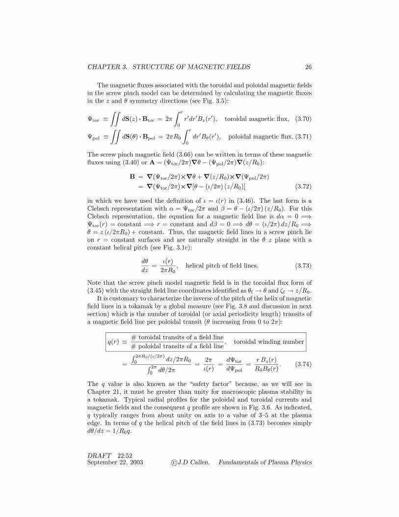
CHAPTER 3. STRUCTURE OF MAGNETIC FIELDS 26
The magnetic fluxes associated with the toroidal and poloidal magnetic fieldsin the screw pinch model can be determined by calculating the magnetic fluxesin the z and θ symmetry directions (see Fig. 3.5):
Ψtor ≡∫∫
dS(z) · Btor = 2π∫ r
0r′dr′Bz(r′), toroidal magnetic flux, (3.70)
Ψpol ≡∫∫
dS(θ) · Bpol = 2πR0
∫ r
0dr′Bθ(r′), poloidal magnetic flux. (3.71)
The screw pinch magnetic field (3.66) can be written in terms of these magneticfluxes using (3.40) or A = (Ψtor/2π)∇θ − (Ψpol/2π)∇(z/R0):
B = ∇(Ψtor/2π)×∇θ + ∇(z/R0)×∇(Ψpol/2π)= ∇(Ψtor/2π)×∇[θ − (ι/2π) (z/R0)] (3.72)
in which we have used the definition of ι = ι(r) in (3.46). The last form is aClebsch representation with α = Ψtor/2π and β = θ − (ι/2π) (z/R0). For thisClebsch representation, the equation for a magnetic field line is dα = 0 =⇒Ψtor(r) = constant =⇒ r = constant and dβ = 0 =⇒ dθ = (ι/2π) dz/R0 =⇒θ = z (ι/2πR0) + constant. Thus, the magnetic field lines in a screw pinch lieon r = constant surfaces and are naturally straight in the θ–z plane with aconstant helical pitch (see Fig. 3.1c):
dθ
dz=ι(r)
2πR0, helical pitch of field lines. (3.73)
Note that the screw pinch model magnetic field is in the toroidal flux form of(3.45) with the straight field line coordinates identified as θf → θ and ζf → z/R0.
It is customary to characterize the inverse of the pitch of the helix of magneticfield lines in a tokamak by a global measure (see Fig. 3.8 and discussion in nextsection) which is the number of toroidal (or axial periodicity length) transits ofa magnetic field line per poloidal transit (θ increasing from 0 to 2π):
q(r) ≡ # toroidal transits of a field line# poloidal transits of a field line
, toroidal winding number
=∫ 2πR0/(ι/2π)0 dz/2πR0∫ 2π
0 dθ/2π=
2πι(r)
=dΨtor
dΨpol=
r Bz(r)R0Bθ(r)
. (3.74)
The q value is also known as the “safety factor” because, as we will see inChapter 21, it must be greater than unity for macroscopic plasma stability ina tokamak. Typical radial profiles for the poloidal and toroidal currents andmagnetic fields and the consequent q profile are shown in Fig. 3.6. As indicated,q typically ranges from about unity on axis to a value of 3–5 at the plasmaedge. In terms of q the helical pitch of the field lines in (3.73) becomes simplydθ/dz = 1/R0q.
DRAFT 22:52September 22, 2003 c©J.D Callen, Fundamentals of Plasma Physics
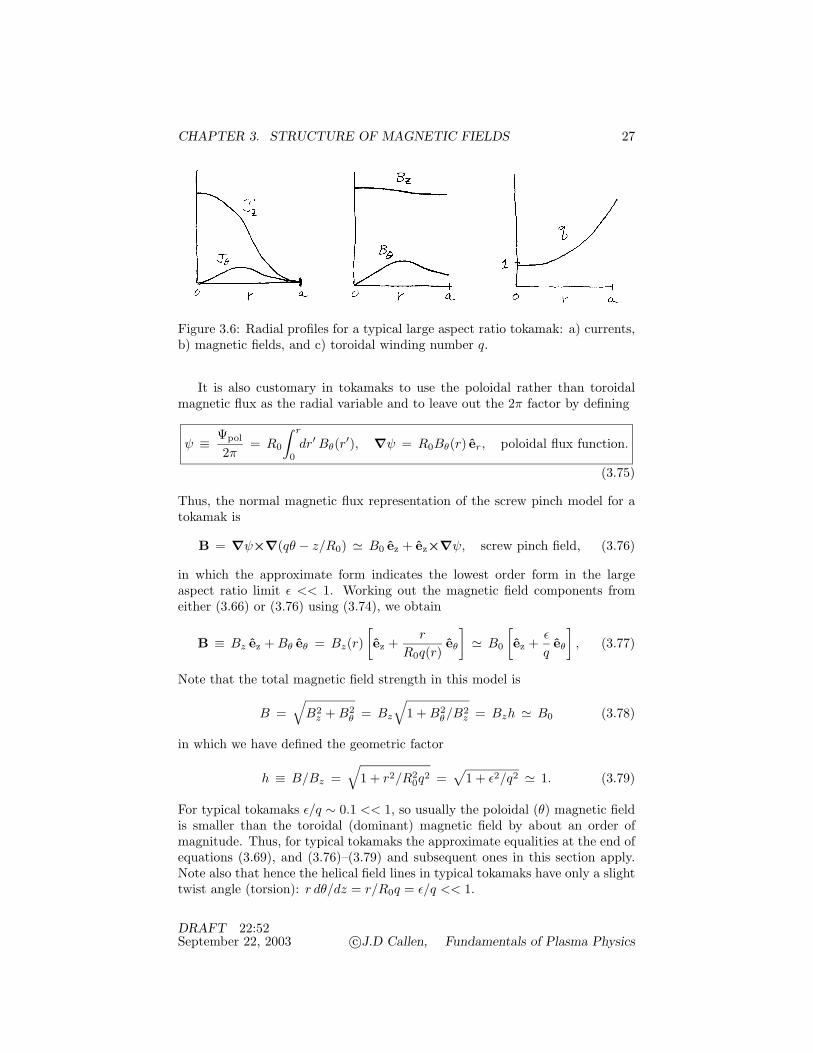
CHAPTER 3. STRUCTURE OF MAGNETIC FIELDS 27
Figure 3.6: Radial profiles for a typical large aspect ratio tokamak: a) currents,b) magnetic fields, and c) toroidal winding number q.
It is also customary in tokamaks to use the poloidal rather than toroidalmagnetic flux as the radial variable and to leave out the 2π factor by defining
ψ ≡ Ψpol
2π= R0
∫ r
0dr′ Bθ(r′), ∇ψ = R0Bθ(r) er, poloidal flux function.
(3.75)
Thus, the normal magnetic flux representation of the screw pinch model for atokamak is
B = ∇ψ×∇(qθ − z/R0) & B0 ez + ez×∇ψ, screw pinch field, (3.76)
in which the approximate form indicates the lowest order form in the largeaspect ratio limit ε << 1. Working out the magnetic field components fromeither (3.66) or (3.76) using (3.74), we obtain
B ≡ Bz ez + Bθ eθ = Bz(r)[ez +
r
R0q(r)eθ
]& B0
[ez +
ε
qeθ
], (3.77)
Note that the total magnetic field strength in this model is
B =√
B2z + B2
θ = Bz
√1 + B2
θ/B2z = Bzh & B0 (3.78)
in which we have defined the geometric factor
h ≡ B/Bz =√
1 + r2/R20q
2 =√
1 + ε2/q2 & 1. (3.79)
For typical tokamaks ε/q ∼ 0.1 << 1, so usually the poloidal (θ) magnetic fieldis smaller than the toroidal (dominant) magnetic field by about an order ofmagnitude. Thus, for typical tokamaks the approximate equalities at the end ofequations (3.69), and (3.76)–(3.79) and subsequent ones in this section apply.Note also that hence the helical field lines in typical tokamaks have only a slighttwist angle (torsion): r dθ/dz = r/R0q = ε/q << 1.
DRAFT 22:52September 22, 2003 c©J.D Callen, Fundamentals of Plasma Physics
CHAPTER 3. STRUCTURE OF MAGNETIC FIELDS 28
In the screw pinch model the magnetic field strength is constant along amagnetic field line; hence from (3.3) the screw pinch model magnetic field unitvectors b ≡ B/B neither converge or diverge. However, the magnetic field inthis model does have torsion, curvature, a perpendicular gradient and shear.For the screw pinch model the unit vector along the magnetic field is
b ≡ BB
=1h
(ez +
r
R0qeθ
)&
(ez +
ε
qeθ
). (3.80)
Using the definition of the torsion in (??) with a unit normal N = ∇ψ/|∇ψ| =er, we find that for the screw pinch model
τ = − (b ·∇)(b×er) = − r
hR0q(eθ ·∇)
eθ
h=
1h2R0q
eθ, torsion. (3.81)
Here, we have used the vector identities (??), (??) and (??) along with ∇θ =eθ/r to show that
(eθ ·∇)eθ = − eθ×(∇×eθ) = − eθ×(∇×r∇θ) = − eθ×(er×eθ)/r = − er/r;(3.82)
hence er · (eθ ·∇)eθ = −1/r. Thus, the distance along a magnetic field line overwhich it twists helically through one radian in the screw pinch model is
Lτ = 1/τr = h2R0q & R0q, torsion length. (3.83)
The torsion vector τ can also be written in terms of the magnetic field com-ponents as τ = (BθBz/rB2) er — see Problem 3.19. Note also that in thetokamak limit of ε/q << 1 the helical pitch of the field lines given in (3.73)becomes simply the torsion τr.
The curvature in the screw pinch model is worked out similarly using thevector identities (??) and (3.82):
κ ≡ (b ·∇)b =r
hR0q(eθ ·∇)
r
hR0qeθ = − r
(hR0q)2er, curvature. (3.84)
The curvature of magnetic field lines in the screw pinch model can be writ-ten in terms of the magnetic field components as κ = −(B2
θ/rB2) er — seeProblem 3.19. The curvature length RC ≡ 1/|κr| = (hR0q)2/r & R0q(q/ε) ismuch longer than the torsion length Lτ & R0q in the screw pinch model of atokamak because the curvature is produced only by the poloidal motion of thesmall pitch helical field lines. The perpendicular (radial) gradient scale length[LB ≡ B/(dB/dr)] is of the order of the curvature radius RC . However, sincethe difference depends on the current and plasma pressure profiles, it will notbe worked out until Chapter 20. Note also that since the curvature is only inthe radial direction there is only normal curvature. Because the magnetic fieldlines do not have curvature within a magnetic flux surface, there is no geodesiccurvature — see (??) in Section D.6.
DRAFT 22:52September 22, 2003 c©J.D Callen, Fundamentals of Plasma Physics
CHAPTER 3. STRUCTURE OF MAGNETIC FIELDS 29
Finally, it can be shown (see Problem 3.25) that for the screw pinch modelthe local magnetic shear defined in (??) and (3.25) becomes (see Problem 3.19for the form of the magnetic shear in terms of the magnetic field componentsBθ and Bz):
ς ≡ (b×er) ·∇×(b×er) =1
LS=
r
h2R0
d
dr
(1q
). (3.85)
Note that in the screw pinch model the shear is constant on a magnetic flux sur-face (r = constant). Recalling from (3.74) that 1/q is just the radian rotationaltransform ι/2π of the helical field lines, the local shear can be written as
ς =1
LS=
r
2πh2R0
dι
dr= − r
h2R0q2
dq
dr= − s
h2R0q& − s
R0q, magnetic shear,
(3.86)
in which
s(r) ≡ r
q
dq
dr, magnetic shear parameter, (3.87)
is an order unity magnetic shear parameter commonly used in stability analysesof tokamak plasmas. There is magnetic shear in large aspect ratio tokamaksonly if the axial current density Jz varies with radius r since ι ∝ Bθ(r)/r ∝(1/r2)
∫ r0 r′dr′Jz(r′). By convention, in tokamak plasma analyses the sign of
the shear is reversed so that s > 0 indicates positive or “normal” magneticshear, and s < 0 indicates reversed or abnormal shear.
Having delineated the local differential properties in the screw pinch model,we can now develop a sheared slab model for it. At finite r since the curvatureand perpendicular gradient scale lengths are so long (compared to the torsionand shear lengths) their effects are usually neglected in the simplest slab models.As indicated previously, the sheared slab model does not include torsion effects.Thus, the local sheared slab model for the screw pinch model of a tokamak neara field line at a radius r0 is simply
Bss = B0 b + b×∇ψaux = B0 [ b + (x/LS) e∧]. (3.88)
in which
ψaux ≡ B0x2
2LS, and e∧ ≡ b×er =
1h
(eθ − ε
qez
)&
(eθ − ε
qez
).
(3.89)
Here, the sheared slab model coordinates x, y, z correspond to r − r0, r0[θ −(ε/q)(z/R0)], z + (ε/q)r0θ and we identify the directions in terms of the cylin-drical coordinate directions through the directions indicated in the unit vector bin (3.80) and a unit vector e∧ that is perpendicular to b within the r = constant(magnetic flux) surface.
The preceding discussion focused on the screw pinch model for tokamaks.The screw pinch model can also be used to represent reversed field pinch (RFP)
DRAFT 22:52September 22, 2003 c©J.D Callen, Fundamentals of Plasma Physics
CHAPTER 3. STRUCTURE OF MAGNETIC FIELDS 30
plasmas. In RFPs the toroidal and poloidal currents are much larger than thosein a tokamak (by a factor ∼ 1/ε ∼ A >> 1). In particular, the poloidal currentJθ is so large that it causes the toroidal magnetic field to reverse direction in theedge of the plasma [see (3.69)] — hence the name of the confinement concept.The toroidal current in an RFP produces a poloidal magnetic field Bθ that isso large that q ∼ ε and the small ε/q expansion that is used for tokamaks isinappropriate. Such a large poloidal magnetic field also produces an order unityhelical pitch of the magnetic field lines; magnetic field lines in an RFP rotatepoloidally and toroidally on about the same length scales, and even become areversed direction helix (q < 0) in the edge of the plasma. For such a magneticfield structure the curvature is clearly dominated by the poloidal motion ofthe field lines; the toroidal curvature effects are higher order. Thus, to lowestorder the general [before the approximate equalities (&)] screw pinch modeldeveloped in this section is often used to approximately describe reversed fieldpinch plasmas. When a more precise description including toroidicity effectsis needed the full magnetic flux description developed in the following sectionmust be used.
3.6 Axisymmetric Toroidal Configurations*
For toroidal magnetic field plasma confinement systems with two magnetic fieldcomponents (toroidal, poloidal) a tremendous simplication occurs when the sys-tem is symmetric in the toroidal direction. Then, axisymmetric magnetic fluxsurfaces are guaranteed to exist and both a Clebsch and flux surface representa-tion are available. The resulting magnetic field system is the simplest, nontrivialtoroidal magnetic field system and is the basic paradigm for all types of toroidalmagnetic confinement systems.
In this section we develop the commonly used axisymmetric toroidal mag-netic field descriptions and coordinate systems in general — without using alarge aspect ratio expansion. We also show the relationship of the descriptionsand coordinates to the large aspect ratio tokamak and screw pinch models. Atthe end of the section we discuss how the general axisymmetric toroidal modelcan be used to describe other axisymmetric toroidal magnetic configurations.
The geometry we consider for an axisymmetric tokamak is shown in Fig. 3.7.Since the toroidal magnetic field is in the direction of axisymmetry (ζ) and∇ζ = eζ/R in which R is the major radius, it can be written as
Btor = Btoreζ = R Btor∇ζ ≡ I ∇ζ, toroidal magnetic field, (3.90)
in which we have defined
I ≡ R Btor, toroidal field function. (3.91)
Because of the axisymmetry, I must be independent of ζ: ∂I/∂ζ = 0. Thetoroidal field function I can be related to the current flowing in the poloidal (θ)direction. The poloidal curent flowing through a disk of (major) radius R that
DRAFT 22:52September 22, 2003 c©J.D Callen, Fundamentals of Plasma Physics

CHAPTER 3. STRUCTURE OF MAGNETIC FIELDS 31
Figure 3.7: Axismmetric tokamak coordinates (ψ, θ, ζ) and geometry for calcu-lating the poloidal current and magnetic flux.
is perpendicular to the axis of symmetry, as shown in Fig. 3.7, is given, usingAmpere’s magnetostatic law ∇×B = µ0J and Stokes’ theorem (??), by
Ipol ≡∫∫
SdS(θ) · J =
∮C
d" · B/µ0 = −∫ 2π
0R dζ Btor/µ0
= − (2π/µ0)RBtor = − (2π/µ0) I. (3.92)
Here, the minus sign occurs because the differential line element on the curveC along the perimeter of the surface S is in the − ζ direction: d" ≡ − eζdζ.Thus, the toroidal field function I represents the poloidal current Ipol flowingin the plasma and coils outside it. For isotropic pressure plasmas I = I(ψ), i.e.,∂I/∂θ = 0.
In the limit of no current flowing in the plasma, the toroidal field functionI is constant and determined by the poloidal currents flowing in the toroidalmagnetic field coils around the plasma. Then, as can be inferred [see (??)] fromthe magnetic field caused by current flowing in an infinite wire on the symmetryaxis (R = 0), the vacuum toroidal magnetic field strength decreases as one over
DRAFT 22:52September 22, 2003 c©J.D Callen, Fundamentals of Plasma Physics

CHAPTER 3. STRUCTURE OF MAGNETIC FIELDS 32
the major radius R:
Btor = I0/R = B0R0/R, vacuum toroidal magnetic field strength, (3.93)
in which B0 and R0 are the magnetic field strength and major radius at themagnetic axis.
Next, we develop a form for the poloidal magnetic field Bpol. Using themagnetic flux definition in (3.36) and taking account of the axisymmetry in thetoroidal (ζ) direction, the poloidal magnetic flux can be written in terms of thetoroidal component of the vector potential (Ator ≡ eζ · A = R ∇ζ · A):
Ψpol =∫∫
SdS(θ) · B =
∮C
d" · A = −∫ 2π
0R dζ Ator = − 2πR Ator. (3.94)
For simplicity in the final tokamak magnetic field represention, it is convenientto define a normalized poloidal magnetic flux function:
ψ ≡ Ψpol/2π = −R Ator, poloidal flux function. (3.95)
Since by definition ∂ψ/∂ζ = 0, the poloidal flux fuction ψ is independent ofthe toroidal angle ζ but in general depends on the cylindrical-like coordinatesin a ζ = constant plane: ψ = ψ(r, θ). In terms of this poloidal flux functionthe toroidal component of the vector potential can be written Ator = −ψ/R,or vectorially as Ator = −(ψ/R) eζ = −ψ∇ζ. Thus, using (3.40), the magneticfield component produced by this magnetic flux becomes
Bpol = ∇×Ator = ∇ζ×∇ψ, poloidal magnetic field. (3.96)
The strength of the poloidal magnetic field is
Bpol = |∇ζ×∇ψ| = |∇ψ|/R, poloidal magnetic field strength, (3.97)
which shows that |∇ψ| = RBpol. The magnetic axis of the tokamak is definedto be where Bpol = 0 and hence ∇ψ = 0.
Adding the two components of the magnetic field, the total magnetic fieldbecomes simply
B = Btor + Bpol = I∇ζ + ∇ζ×∇ψ, axisymmetric magnetic field.(3.98)
While this form is quite compact, it is unfortunately in neither a Clebsch formnor a two component magnetic flux form. Also, it is not written in terms ofstraight-field-line coordinates, and it is a mixed covariant and contravariantform — see Section D.8. Nonetheless, because this representation is compactand rigorously valid it is heavily used in analyses of axisymmetric toroidal andin particular tokamak plasmas.
Since by axisymmetry the poloidal flux function must be independent of thetoroidal angle (i.e., ∂ψ/∂ζ = 0), taking the dot product of B with ∇ψ we obtain
B ·∇ψ = (Btor + Bpol) ·∇ψ = I∇ζ · ∇ψ + ∇ζ×∇ψ ·∇ψ = 0. (3.99)
DRAFT 22:52September 22, 2003 c©J.D Callen, Fundamentals of Plasma Physics

CHAPTER 3. STRUCTURE OF MAGNETIC FIELDS 33
Thus, the poloidal flux function ψ satisfies the flux surface condition (3.37);hence, magnetic field lines in axisymmetric toroidal systems lie on ψ = con-stant surfaces and ψ will be a convenient magnetic flux surface label and radialcoordinate. Note that, by construction and because of axisymmetry, ψ is a suit-able magnetic flux function for both the toroidal and poloidal magnetic fields.Thus, we can develop a combined magnetic fluxes and Clebsch magnetic fieldrepresentation like (3.45) based on it.
So far we have identified two useful curvilinear coordinates for describingthe tokamak magnetic field: the axisymmetry angle ζ for the toroidal angle andthe poloidal magnetic flux function ψ for the “radial” variable. Next, we needto identify a useful poloidal angle variable. We would like to have a poloidalangle coordinate in which magnetic field lines are straight. Thus, we would likea poloidal angle such that the magnetic field representation could be put in thecombined Clebsch and magnetic flux representation given by (3.45), with ι/2πreplaced by 1/q and Ψtor/2π replaced by ψ for a tokamak representation.
In order to put the tokamak magnetic field (3.98) in the form of (3.45), thetoroidal magnetic field (3.90) must be put into the straight-field-line form
Btor = ∇ψ×∇(qΘ) =⇒ B = ∇ψ×∇(qΘ− ζ) (3.100)
in which θf → Θ (tokamak convention) is the desired straight field line poloidalangle. Taking the dot product of the two forms of Btor given in (3.90) and(3.100) with ∇ζ and equating them, we obtain
Btor · ∇ζ = I∇ζ · ∇ζ = I/R2
= ∇ψ×∇(qΘ) · ∇ζ = q (∇ζ×∇ψ) · ∇Θ = q Bpol · ∇Θ (3.101)
in which we have used ∇q×∇ψ = 0 [because q is only a function of ψ — see(3.105) below] and the order of the vector operations has been rearranged using(??) and (??). Equating the results on the two lines of (3.101), we find
Bpol · ∇Θ = I/qR2 = B · ∇Θ, (3.102)
where the last equality follows from the fact that since by axisymmetry theangle Θ must be independent of ζ, Btor · ∇Θ = 0; thus, B · ∇Θ = Bpol · ∇Θ.Defining a differential length d!pol in the poloidal direction on a magnetic fluxsurface, the last form of (3.101) yields
∂Θ∂!pol
=1
B · ∇!pol
I
qR2=⇒ Θ =
1q
∫ !pol d!pol
B · ∇!pol
I
R2, (3.103)
in which the integration is to be performed at constant ψ, ζ. The poloidal lengthvariable !pol can be defined in terms of the ordinary cylindrical angle θ about themagnetic axis. Taking the dot product of the field line equation (3.28) with ∇θand ∇!pol, we find that the poloidal length variable is related to the cylindricalangle bydx · ∇θ
d!=
B · ∇θB
,dx · ∇!pol
d!=
B · ∇!pol
B=⇒ dθ
B · ∇θ =d!pol
B · ∇!pol.
(3.104)
DRAFT 22:52September 22, 2003 c©J.D Callen, Fundamentals of Plasma Physics

CHAPTER 3. STRUCTURE OF MAGNETIC FIELDS 34
Integrating the last form of (3.103) over one complete poloidal traversal ofthe flux surface, which we define to be Θ = 2π, we obtain an expression for thetoroidal winding number:
q(ψ) =12π
∮d!pol
B · ∇!pol
I
R2=
12π
∮dθ
B · ∇θI
R2
or,
q(ψ) =12π
∮dθ
B · ∇ζB · ∇θ & 1
2π
∮dθ
rBtor
RBpol& rBtor
RBpol[1 + Oε2]. (3.105)
Here, we have used I/R2 = B · ∇ζ from (3.101) and indicated in the approxi-mate equalities (here and below) the forms that result in the large aspect ratiolimit (ε << 1). Note that the lowest order, approximate form for q agrees withthe screw pinch model result (3.74).
The toroidal winding number q may be an integer or the ratio of two integers(e.g., q = m/n); then, a magnetic field line on that surface would close on itselfafter an integer number of poloidal (n) and toroidal (m) transits around thetorus — see (3.74) and Fig. 3.8. Such a surface is called a rational surface.All magnetic field lines on a rational surface rotate with the same rotationaltransform ι, running forever parallel to adjacent field lines on the flux surface;hence, they sample only a given field line on the flux surface. On the other hand,if q is not the ratio of two integers, then the flux surface is called irrational. Thus,we define (see Fig. 3.8)
q(ψ) = m/n, rational flux surface,
q(ψ) -= m/n, irrational flux surface,(3.106)
in which m, n are integers. Magnetic field lines on an irrational flux surfacedo not close on themselves; however, if they are followed long enough, theyfill the entire flux surface. This is called ergodic behavior since all points onthe surface are then equally sampled — at least statistically in an asymptoticlimit. Note that the vast majority of flux surfaces are irrational; they form adense set. Rational surfaces are “infrequent,” separated radially (i.e., in ψ) andof measure zero. Nonetheless, they are very important in magnetized toroidalplasmas because physical processes taking place on adjacent rational field linesare mostly isolated from each other, and because they are degenerate field linesthat are especially vulnerable to resonant nonaxisymmetric perturbations thatcan produce magnetic island structures like those discussed in Section 3.3.
An explicit expression for Θ will now be obtained. Using the rigorous formof the definition of q in (3.105) and defining Θ like the simple geometric angleθ to be zero on the outer midplane of the torus, we can develop from (3.104)explicit expressions for the straight-field-line poloidal angle:
Θ ≡ 1q
∫ !θ
0
d!θB · ∇!θ
I
R2=
1q
∫ θ
0
dθ
B · ∇θI
R2=
1q
∫ θ
0dθ
B · ∇ζB · ∇θ . (3.107)
DRAFT 22:52September 22, 2003 c©J.D Callen, Fundamentals of Plasma Physics

CHAPTER 3. STRUCTURE OF MAGNETIC FIELDS 35
Figure 3.8: “Puncture plots” of magnetic field lines in a ζ = constant plane ona magnetic flux surface in an axisymmetric torus. The numbers listed indicatethe number of toroidal transits executed by a field line. On rational surfacesfield lines retrace the same trajectory after m toroidal transits whereas on anirrational surface a single field line is ergodic and (eventually) samples the entiresurface.
It can be shown using steps like the last few ones in (3.105) that, to lowest orderin a large aspect ratio expansion (e.g., near the magnetic axis), the straight fieldline coordinate Θ is equal to the local cylindrical coordinate θ:
Θ = θ −Oε sin θ. (3.108)
The order ε sinusoidal variations of Θ with θ depend on the currents flowingin the plasma; their evaluation will be deferred until Chapter 20 where we usethe macroscopic force balance equations in a finite-pressure tokamak plasma todetermine the currents in a tokamak plasma and the shape of the ψ(x) surfaces.
As can be seen from Fig. 3.1d, the magnetic field in a tokamak has paralleland perpendicular gradients, curvature (both normal and geodesic), and localtorsion and shear that are not constant along the magnetic field. Below, we willgive general expressions for each of these properties both in general, and also intheir lowest order forms in a large aspect ratio (ε << 1), low plasma pressureexpansion. To lowest (zeroth) order the magnetic flux surfaces become circlesabout the magnetic axis. (To first order in ε the flux surfaces are still circles, buttheir centers are shifted outward slightly in major radius — see Section 20.4.)Thus, to lowest order we will use the r, θ, z coordinates of a cylinder whose zaxis lies on the magnetic axis of the tokamak, of a type shown in Fig. 3.1d. Tolowest order the model will mostly reduce to the screw pinch model discussedin the preceding section — compare Fig. 3.5 with Fig. 3.7.
The major radius R to any point in the plasma will be given in terms of the
DRAFT 22:52September 22, 2003 c©J.D Callen, Fundamentals of Plasma Physics

CHAPTER 3. STRUCTURE OF MAGNETIC FIELDS 36
major radius of the magnetic axis (R0) and the local cylindrical coordinates by
R = R(ψ,Θ) & R0 [ 1 + ε cos θ + Oε2]. (3.109)
Using this approximate representation in the equation for the vacuum magneticfield strength variation with R given in (3.93) and the fact that in our tokamakmodel B & Btor [ 1 + Oε2/q2], we obtain
B = B(ψ,Θ) & B(r, θ) & B0 [ 1 − ε cos θ + Oε2], tokamak field strength.
(3.110)
The magnetic field strength in a tokamak varies approximately sinusoidallyalong a helical magnetic field line from its minimum on the outside (θ = 0 whereBmin/B0 & 1− ε) to its maximum on the inside (θ = π where Bmax/B0 & 1+ ε)of the torus. Thus, it can be represented by the sinusoidal model in (3.6) using! → R0q θ and L! → 2πR0q. The magnitude of the variation along a magneticfield line is usually small: ∆B ≡ Bmax −Bmin & 2εB0 << B0. Hence, the mag-netic mirror ratio defined in (3.7) is usually only slightly greater than unity:Rm ≡ Bmax/Bmin & 1 + 2ε. In summary, the variation of the magnetic fieldstrength along field lines in large aspect ratio tokamaks can be modeled by (3.6)with
Bmin & (1 − ε)B0, ∆B & 2εB0, !→ R0q θ, L! → 2πR0q,
tokamak Bsin model parameters. (3.111)
To calculate the perpendicular gradient, curvature and shear in the tokamakmagnetic field we need to explicitly relate the tokamak magnetic flux systemcoordinates ψ,Θ, ζ, which are unfortunately not orthogonal (∇Θ · ∇ψ -= 0), tothe local cylindrical coordinates (r, θ, z) about the magnetic axis:
∇ψ & BpolR ∇r & BpolR0 er, ψ(r) &∫ r
0dr BpolR0, (3.112)
∇Θ & ∇θ & eθ
r, B ·∇Θ =
I
qR2& Bpol
r& B0
R0q, (3.113)
∇ζ =eζ
R& eζ
R0[ 1 − ε cos θ + Oε2]. (3.114)
The poloidal magnetic field strength oscillates slightly with poloidal angle:
Bpol ≡ |∇ψ|/R & (ε/q)B0 [ 1 + Oε cos θ]. (3.115)
In calculating gradients of various quantities in tokamak system coordinates,we just use chain rule differentiation:
∇⊥B
B=
1B
(∇ψ∂B∂ψ
+ ∇⊥Θ∂B
∂Θ
)& 1
R0[− er cos θ + eθ sin θ + Oε] .
(3.116)
DRAFT 22:52September 22, 2003 c©J.D Callen, Fundamentals of Plasma Physics

CHAPTER 3. STRUCTURE OF MAGNETIC FIELDS 37
in which we have used (3.93) and ∂/∂ζ terms vanish by axisymmetry. In a toka-mak with low plasma pressure and hence a small poloidal current (see Chapter20) the J×B contribution to the curvature is small. Thus, using (3.20) thecurvature is given by
κ =∇⊥B
B+ µ0
J×BB2
& 1B
(∇ψ ∂B
∂ψ+ ∇⊥Θ
∂B
∂Θ
)& 1
R0[− er cos θ + eθ sin θ + Oε] , tokamak curvature vector. (3.117)
To this lowest order the curvature is simply the toroidal curvature of the system.Note that a tokamak has both normal (perpendicular to the flux surface, κN &κr = − cos θ/R0) and geodesic (within the flux surface, κB & κθ = sin θ/R0)curvature — see Section D.6. Note further that, because of the inclusion oftoroidicity effects, the tokamak curvature is one order in ε larger than that inthe screw pinch model (3.84); however, its sign oscillates with the poloidal angleθ and its average is of the same order as the curvature in the screw pinch model.To determine the Oε terms in (3.117) we need to take account of the plasmapressure and current profiles in the tokamak — see Chapter 20.
Using a number of vector identities and other manipulations (see Problem3.29), it can be shown that the normal torsion in a tokamak can be written as
τN =I |∇ψ|B2R
(B ·∇Θ)[∂
∂ψ
(qR|∇ψ|
I
)+∂
∂Θ
(qR|∇ψ|
I
∂Θ∂ψ
)]& 1
R0q[ 1 + Oε cos θ], tokamak local torsion, (3.118)
which to the lowest order is the same as in the screw pinch model — see (3.81).Similarly, the magnetic shear in a tokamak becomes (see Problem 3.31):
ςy = − |∇ψ|2B2
(B ·∇)[∂
∂ψ(qΘ)
]= − |∇ψ|2
B2(B ·∇Θ)
[dq
dψ+ q
∂
∂Θ
(∂Θ∂ψ
)]& − 1 + O(ε cos θ)
R0q[ s −Oε cos θ], tokamak local shear, (3.119)
which again to lowest order is the same as in the screw pinch model — see(3.86). [The convention in the tokamak literature is to reverse the sign of theshear — so that it is positive for normal tokamaks in which q increases withradius (see Fig. 3.6).] Note that both the local torsion and local shear have orderε sinsoidal variations along a magnetic field line as it moves from the outside toinside of the torus — but their averages over a magnetic flux surface (i.e., overθ) are approximately given by their respective values in the screw pinch model.Again, to obtain the next order (ε) terms correctly we need to take account ofplasma currents and pressures, which we defer until Chapter 20.
In this section we have developed the magnetic field representation and prop-erties of axisymmetric toroidal magnetic field systems in general, and then in-dicated the lowest order results in the large aspect ratio expansion (ε ≡ r/R0 =
DRAFT 22:52September 22, 2003 c©J.D Callen, Fundamentals of Plasma Physics
CHAPTER 3. STRUCTURE OF MAGNETIC FIELDS 38
1/A << 1) after an approximate equality sign (&). While the discussion has fo-cused on the tokamak magnetic field structure, the general development appliesto any axisymmetric toroidal system. Thus, it applies to spherical tokamaks[very low aspect ratio (A ∼ 1.1–1.5) tokamaks], spheromaks [effectively unityaspect ratio tokamaks without toroidal field coils] and reversed field pinches[effectively tokamaks with very low q ∼ ε << 1]. For spherical tokamaks andspheromaks the full generality of the magnetic flux coordinates must be usedbecause a large aspect ratio expansion is invalid — except for small radius fluxsurfaces near the magnetic axis where a large aspect ratio expansion can beused. As indicated at the end of the preceding section, the general screw pinchmodel represents reversed field pinches except for the purely toroidal effects(variation of B from the outer to inner edge of the torus and toroidal curva-ture of field lines). These latter effects are included in the general magneticflux model developed in this section. In summary, the general magnetic fluxsurface model developed in this section is appropriate for describing all types ofaxisymmetric toroidal magnetic field configurations — tokamaks, reversed fieldpinches, spherical tokamaks, and spheromaks.
3.7 Local Expansion of a Magnetic Field+
In order to develop a comprehensive picture of all the possible first derivativeproperties of a magnetic field, in this section we carry out a formal Taylor seriesexpansion of the magnetic induction vector field B(x). The expansion will becarried out at an arbitrary point in the magnetic configuration where the originof a local Cartesian coordinate system will be placed. Thus, our local Taylorseries expansion (subscript le) becomes
Ble(x) = B0 + x ·∇B0 + . . . , (3.120)
in which B0 is the magnetic induction field at the chosen point, x is the vectordistance from this point, and ∇B0 represents the evaluation of the tensor ∇B atthis point. The second and higher order terms in (3.120) will be neglected sincewe are interested here only in the local properties of non-pathological magneticfields for which the first derivatives provide a sufficient description.
This section uses a number of vector differentiation identities and seeks toconnect the local magnetic field derivatives to the common definitions of mostof these properties for arbitrary vector fields. These subjects are summarizedbriefly in Appendix D, and in particular in the Section D.6. Readers are en-couraged to read the relevant sections in Appendix D in conjunction with thissection.
As usual we decompose the magnetic induction field B(x) into its vectordirection and scalar magnitude components at any spatial point x by writing
B(x) = B b = B(x) b(x), (3.121)
DRAFT 22:52September 22, 2003 c©J.D Callen, Fundamentals of Plasma Physics
CHAPTER 3. STRUCTURE OF MAGNETIC FIELDS 39
in which
B(x) ≡ |B(x)| =√
B · B, magnetic field strength, (3.122)b(x) ≡ B(x)/B(x) = B/B, unit vector along B(x). (3.123)
Using this decomposition, we can write the tensor ∇B0 as
∇B0 ≡ (∇B b)0 = b0∇B0 + B0∇b0, (3.124)
in which b0 is the unit vector b evaluated at the origin (point of interest) and∇B0, ∇b0 are ∇B, ∇b evaluated at this same point.
To work out the various components of the ∇b and hence ∇B tensors wecan use a local Cartesian coordinate system whose z axis is aligned along bat x = (0, 0, 0) (i.e., b0) and which has its x axis in a particular directionperpendicular to b0, which we will specify later. Thus, the orthonormal triadof unit vectors characterizing this local coordinate system will be ez = b0, ex,ey ≡ b0×ex. For notational simplicity, in what follows we omit the subscriptzero on the magnetic field unit vector b.
Consider first the components locally parallel to the magnetic field:
(∇b)zz ≡ b · (b ·∇)b = − b · b×(∇×b) = 0,(∇b)zx ≡ [(b ·∇)b] · ex = ex· (b ·∇)b -= 0,(∇b)zy ≡ [(b ·∇)b] · ey = ey· (b ·∇)b -= 0,(∇b)xz ≡ b · (ex·∇)b = 1
2 (ex·∇)(b · b) = 0,(∇b)yz ≡ b · (ey·∇)b = 1
2 (ey·∇)(b · b) = 0,
(3.125)
in which we have used the fact that since b is a unit vector, we have b · b = 1,and the vector identity,
12
∇(b · b) = 0 = b×(∇×b) + (b ·∇)b. (3.126)
For the components locally perpendicular to the magnetic field we have
(∇b)xx ≡ ex· (ex·∇)b,(∇b)yy ≡ ey· (ey·∇)b,(∇b)xy ≡ ey· (ex·∇)b = + ey·∇×ey − ex· (b ·∇)ey,(∇b)yx ≡ ex· (ey·∇)b = − ex·∇×ex + ex· (b ·∇)ey,
(3.127)
in which we have worked out the last two cross terms using vector differentiationidentities (??) and (??) as follows:
ey· (ex·∇)b = ey· [−∇×(ex×b) + ex(∇· b) − b (∇· ex) + (b ·∇)ex]= ey·∇×ey + ey· (b ·∇)ex = ey·∇×ey − ex· (b ·∇)ey,
(3.128)
and similarly for (∇b)yx.
DRAFT 22:52September 22, 2003 c©J.D Callen, Fundamentals of Plasma Physics
CHAPTER 3. STRUCTURE OF MAGNETIC FIELDS 40
Taking the derivative of the equation along a magnetic field line given in(3.28) yields the second derivative of the field line’s coordinate and hence thelocal curvature of the magnetic field [d/d! ≡ (b ·∇)]:
κ ≡ d2b(!)d!2
= (b ·∇)b = − b×(∇×b), curvature vector, (3.129)
which is perpendicular to the local magnetic field (b · κ = 0). The zx, zycomponents of the tensors ∇b can be written in terms of the x, y componentsof the curvature vector:
(∇b)zx = ex· (b ·∇)b = ex· κ ≡ κx,(∇b)zy = ey· (b ·∇)b = ey· κ ≡ κy.
(3.130)
The x component of the curvature vector is the same as the κx in the shearedslab model given by (3.16) and (3.21). From geometrical considerations theradius of the curvature vector RC is antiparallel to the curvature vector κ.Hence it is given by
RC = −κ/κ2, or κ = −RC/R2C , radius of curvature. (3.131)
The torsion of a vector field is by convention defined to be the negative of theparallel derivative of the binormal vector, which for our geometry is b×ex = ey:
τ = − (b ·∇) (b×ex) = − (b ·∇) ey, torsion vector. (3.132)
The x component of this vector is given by
τx ≡ − ex· (b ·∇)ey = ey· (b ·∇)ex, (3.133)
which is a quantity that appears in xy and yx components of the tensor ∇b.Physically, the torsion vector measures the change in direction (or twist) of thebinormal b×ex as one moves along the magnetic field.
Shear of a vector field can be defined for the two directions perpendicular tothe magnetic field by
ςx ≡ ex·∇×ex = (b×ey) ·∇×(b×ey), shear in surface perpendicular to x,(3.134)
ςy ≡ ey·∇×ey = (b×ex) ·∇×(b×ex), shear in surface perpendicular to y.(3.135)
That these quantities represent the local shear in the vector field B can beseen by realizing that, for example, b×ex represents the surface locally per-pendicular to ey, ∇×(b×ex) represents the tangential motion (see Fig. ??) ordifferential twisting of this surface, and (b×ex) ·∇×(b×ex) is the componentof this differential twisting in the original direction ey. Note that if ex (or ey)
DRAFT 22:52September 22, 2003 c©J.D Callen, Fundamentals of Plasma Physics

CHAPTER 3. STRUCTURE OF MAGNETIC FIELDS 41
were a unit vector corresponding to a contravariant base vector ∇ui in a curvi-linear coordinate system (see Section D.8), then ei = ∇ui/|∇ui| and hence ςi ≡ei·∇×ei = (∇ui·∇×∇ui)/|∇ui|2 = 0. Thus, there is no shear in a directiondescribed by the gradient of a scalar function (e.g., a magnetic flux function) —because the gradient of a scalar is an irrotational quantity (∇×∇f = 0). Thecorresponding parallel “shear” b ·∇×b (or parallel component of the vorticityin the vector field B) can be written in terms of the x component of the torsionvector and the two perpendicular shear components as follows:
ςz ≡ b ·∇×b = 2 τx + ςx + ςy, parallel component of vorticity in B field.(3.136)
In the absence of shear, this relation is analogous to the component of rotationof a rigidly rotating fluid in its direction of flow, i.e., 1
2V·∇×V.The xy and yx or cross components of the ∇b tensor can be written in
terms of the x, y components of the torsion and shear as follows:
(∇b)xy = ςy + τx,(∇b)yx = ςx + τx.
(3.137)
The divergence of the unit vector b can be written as [using (??)]
∇· b = ex· (ex·∇)b + ey· (ey·∇)b +
0︷ ︸︸ ︷b · (b ·∇)b . (3.138)
Thus, the xx and yy (or diagonal matrix element) components of the ∇b tensorrepresent the x and y components of the divergence of the unit vector b. Wedefine these divergence (δ) components of the vector field B as follows:
δx ≡ ex· (ex·∇)b = (1/B)[ex· (ex·∇)B],
δy ≡ ey· (ey·∇)b = (1/B)[ey· (ey·∇)B].(3.139)
Collecting together the various components of the tensor ∇b we thus find,in matrix form,
∇b = (ex ey b)
δx τx + ςy 0−τx − ςx δy 0κx κy 0
ex
ey
b
. (3.140)
Further, using this result in (3.124), we find that the tensor ∇B can be similarlywritten as
∇B ≡(ex ey b
) ∂Bx/∂x ∂By/∂x ∂Bz/∂x∂Bx/∂y ∂By/∂y ∂Bz/∂y∂Bx/∂z ∂By/∂z ∂Bz/∂z
ex
ey
b
= B0
(ex ey b
) δx τx + ςy γx−τx − ςx δy γyκx κy δz
ex
ey
b
,
(3.141)
DRAFT 22:52September 22, 2003 c©J.D Callen, Fundamentals of Plasma Physics
CHAPTER 3. STRUCTURE OF MAGNETIC FIELDS 42
in which the differential parameters of the magnetic field, including some newgradient (γ) ones which we have introduced here, are defined by:
δx ≡ 1B [ex· (ex·∇)B], δy ≡ 1
B [ey· (ey·∇)B],δz ≡ 1
B (b ·∇)B, divergence,κx ≡ ex· (b ·∇)b, κy ≡ ey· (b ·∇)b, curvature,τx ≡ −ex· (b ·∇)ey, τy ≡ −ey· (b ·∇)ex = −τx, torsion,ςx ≡ ex·∇×ex, ςy ≡ ey·∇×ey, shear,γx ≡ ex·∇ lnB, γy ≡ ey·∇ lnB,γz ≡ b ·∇ lnB0 = δz, gradient B.
(3.142)
Using the expression for ∇B in (3.120) yields the following Taylor series expan-sion for the magnetic induction field B:
Ble & B0 [ b ( 1 + x ·∇ lnB) lowest order + gradient (∇B)+ z κ curvature, κ ≡ (b ·∇)b = κxex + κyey
+ τx (x ey − y ex) torsion, x ey − y ex = 12 b×∇(x2 + y2)
+ (x ςyey − y ςxex) shear+ (x δxex + y δyey) ] divergence
(3.143)
= B0 [ b ( 1 + xγx + yγy + zγz)+ ex(zκx − yτx − yςx + xδx) + ey(zκy + xτx + xςy + yδy)].
Note that this general result simplifies to the sheared slab model (3.8) when theparameters γy, γz, κy ςx, τx, δx, δy and δz all vanish, i.e., when the magneticfield does not vary in the y, z directions, and there is no shear in the x directionand no torsion of the magnetic field lines.
The solenoidal condition (∇· B = 0) will be satisfied by this local expansionas long as
0 =1B
∇· Ble =1B
[ex·(ex·∇)B] +1B
[ey·(ey·∇)B] + b ·∇ lnB = δx + δy + δz.
(3.144)
Thus, the three diagonal components of the matrix of ∇B tensor elements arenot independent; there are only 8 independent components of the ∇B tensor.
The curl of our local approximation of the magnetic induction field B isgiven by
∇×Ble = B0 [ b×(−∇ lnB + κ) + b (b ·∇×b) ], (3.145)
in which we have made use of (3.136). As in the sheared slab model, for plasmaequilibrium situations where the magnetostatic Ampere’s law applies, the cur-rents flowing in the plasma provide further constraint relations between thevarious local differential parameters involved in (3.145). In particular, since cur-rents perpendicular to magnetic fields are typically small, usually κ & ∇⊥ lnB
DRAFT 22:52September 22, 2003 c©J.D Callen, Fundamentals of Plasma Physics
CHAPTER 3. STRUCTURE OF MAGNETIC FIELDS 43
≡ −b×(b×∇ lnB), i.e., the curvature vector is approximately equal to theperpendicular gradient of the magnetic field strength. Also, the parallel “shear”(parallel component of vorticity in the magnetic field b ·∇×b = µ0B · J/B2) isnonzero only if current flows along the magnetic field, i.e, B · J -= 0.
The curvature, shear and perpendicular gradient properties of a magneticfield were discussed in the context of the sheared slab model in Section 3.1.They are illustrated in Fig. 3.2 and their effects mathematically described in(3.14) and (3.24). The additional magnetic field line properties of torsion anddivergence can be understood as follows.
Eliminating all but the torsion terms in (3.143), the x, y, z equations govern-ing the trajectory of a magnetic field line deduced from (3.28) become simply
dx
d!= − y τx,
dy
d!= x τx,
dz
d!= 1 =⇒ ! = z.
Dividing the second equation by the first yields
dy
dx= − x
y=⇒ d (x2 + y2) = 0,
whose solution is
x2 + y2 = x20 + r2
0 ≡ r20 = constant.
This result can be used to reduce the equation for dx/d! = dx/dz to one in onlytwo variables:
dx
dz= − y τx = − (r2
0 − x2)1/2τx =⇒ arcsinx
r0= − z τx + constant.
The equations governing a field line with torsion τx that passes through thepoint x0, y0 are thus given by
x = r0 sin(−zτx + ϕ0), y = r0 cos(−zτx + ϕ0), ϕ0 ≡ arctan(y0/x0).(3.146)
These equations show that torsion means that as one moves along a magneticfield line it undergoes circular motion through an angle of one radian in an axialdistance of τ−1
x ≡ Lτ in the plane perpendicular to the magnetic field — seeFigure 3.9a. Comparing the field line trajectory equations for torsion with thatderived previously for shear, (3.24), or Fig. 3.9a with 3.9b, we see that whereastorsion represents “rigid body” rotation or twisting of the field lines in theplane perpendicular to the magnetic field, shear (ςx = 0, ςy -= 0 for Fig. 3.2b)represents differential twisting of field lines out of a plane (the x–z plane forςy -= 0). Thus, whereas the torsion terms can be removed by transforming to arotating coordinate system, the effects of magnetic shear cannot be removed bysuch coordinate transformations.
To explore the divergence of magnetic field lines we eliminate all but the δxand δz terms in (3.143), and take δz = − δx so as to satisfy the solenoidal con-dition (3.144). Then, the equations governing the magnetic field line trajectory
DRAFT 22:52September 22, 2003 c©J.D Callen, Fundamentals of Plasma Physics

CHAPTER 3. STRUCTURE OF MAGNETIC FIELDS 44
Figure 3.9: Additional magnetic field line characteristics. In each sketch thenature of magnetic field lines are indicated when only the identified coefficient(s)do not vanish.
in the x–z plane become
dx
d!= x δx,
dz
d!& 1.
Integrating the first equation a short distance (z δx << 1) along the magneticfield line that passes through the point x = (x0, 0, 0) yields
x(z) = x0 eδxz = x0 e−δzz = x0 exp[− z
d lnB
dz
]& x0 B(0)
B(z). (3.147)
This result shows that the divergence (δx > 0) in the x–z plane (cf., Fig. 3.9b)is accompanied by a decrease in the magnetic field strength [δz ≡ d lnB/dz < 0,B(z) < B(0) for z > 0], as is required by the solenoidal condition ∇· B = 0 —see (3.2) and (3.144). The divergence scale length δ−1
x (or equivalently |δz|−1)is the linear extrapolation distance along a field line over which the density ofmagnetic field lines would decrease (increase for δx < 0, δz > 0) in magnitudeby a factor of two and the field lines diverge (converge) by a factor of e.
We can also develop a Taylor series expansion of the magnetic induction fieldB(x) about a given magnetic field line. Here, we define x⊥ = −b×(b×x) as the“small” vectorial distance off a given magnetic field line in the x, y plane locallyperpendicular to the field line. The axial distance along the magnetic field lineis parameterized by the length ! along it from an initial reference point. Thus,
DRAFT 22:52September 22, 2003 c©J.D Callen, Fundamentals of Plasma Physics

CHAPTER 3. STRUCTURE OF MAGNETIC FIELDS 45
the desired expansion is
Ble(x⊥, !) = B0(!) b0(!) + x⊥·∇B0(!)
= B0(!)(b0(!) [ 1 + x⊥·∇ lnB0(!) ]
+ 12τxb0(!)×∇(x2 + y2) + [x ςyey − y ςxex] + [x δxex + y δyey]
)(3.148)
in which all quantities are now evaluated on a particular field line (i.e., atx⊥ = 0), but the functional dependence on ! remains. Compared to the expan-sion about a point given in (3.143), we see that the curvature (κ) and parallelgradient (γz) or divergence (δz) terms are missing from the expansion about afield line — because these effects are included via b0(!) and B0(!). Note alsothat this field line expansion for B satisfies the solenoidal condition ∇· B = 0 aslong as (3.144) is satisfied, and yields the result given in (3.145) for ∇×B. Sincecharged particles in a plasma usually move much more easily (and hence traversemuch longer distances) along magnetic field lines than perpendicular to them,the expansion about a field line is usually more useful, at least conceptually, forplasma physics applications.
As discussed in Sections 3.2, 3.4–3.6, often in plasma physics there exista set of nested magnetic flux surfaces ψ(x) that surround nested bundles ofmagnetic field lines. When such surfaces exist, ∇ψ is locally perpendicular tothe magnetic field and it can be used to specify the directions of the unit vectorsin the plane locally perpendicular to the magnetic field:
ex ≡ ∇ψ/|∇ψ|, ey ≡ b×∇ψ/|b×∇ψ| = b×∇ψ/|∇ψ|. (3.149)
For such cases it is customary to call the curvature component in the directionperpendicular to the magnetic flux surfaces (i.e., in the ∇ψ direction) the normalcurvature and the curvature component within the magnetic flux surface (i.e.,in the b×∇ψ direction) the geodesic curvature:
κx = κψ ≡ κ ·∇ψ/|∇ψ|, normal (∇ψ) curvature,
κy = κb×∇ψ ≡ κ · b×∇ψ/|∇ψ|, geodesic (b×∇ψ) curvature.(3.150)
Since this x coordinate direction is in the direction of the gradient of a scalar,the shear in the x direction vanishes: ςx = ∇ψ ·∇×∇ψ/|∇ψ|2 = 0. However,there can still be shear in the y direction; it can be written as
ςy =(b×∇ψ) ·∇×(b×∇ψ)
|b×∇ψ|2 , shear for ex ∝ ∇ψ. (3.151)
The torsion for this situation where magnetic flux surfaces are assumed to existcan be written as
τx = − ∇ψ · (b ·∇)(b×∇ψ)|∇ψ|2 , torsion for ex ∝ ∇ψ. (3.152)
DRAFT 22:52September 22, 2003 c©J.D Callen, Fundamentals of Plasma Physics

CHAPTER 3. STRUCTURE OF MAGNETIC FIELDS 46
Using these relations in (??) along with the fact that for ex ∝ ∇ψ we haveςx ≡ ex·∇×ex = (∇ψ/|∇ψ|) ·∇×(∇ψ/|∇ψ|) = 0, we can write the parallelshear in the magnetic field as
σ ≡ b ·∇×b = µ0B · J/B2 = ςy + 2 τx, parallel shear for ex ∝ ∇ψ.(3.153)
Note that this relation provides a relationship between the parallel current andthe torsion and shear in the magnetic field. It is the parallel current analogyto the relationship between the curvature vector, ∇⊥ lnB and perpendicularcurrent given in (3.20). Finally, the x and y field line divergence parameterscan be written as
δx = − b · (ex·∇)ex = (b×ex) ·∇(|∇ψ|−1)×∇ψ = − (b ·∇) ln |∇ψ|, (3.154)
δy = − δx − δz = (b ·∇) ln |∇ψ|− (b ·∇) lnB, divergences with ex ∝ ∇ψ.(3.155)
These simplified formulas for the situation where the x coordinate is taken tobe in the magnetic flux surface gradient direction are the most commonly usedones in plasma physics.
REFERENCES AND SUGGESTED READINGPlasma physics books that discuss some aspects of the structure of magnetic fields
include
Bittencourt, Fundamentals of Plasma Physics, Chapt. 3 (1986) [?]
Hazeltine and Meiss, Plasma Confinement, Chapt. 3 (1992) [?]
Miyamoto, Plasma Physics for Nuclear Fusion, Chapt. 2 (1980) [?]
Schmidt, Physics of High Temperature Plasmas (1966,79) [?]
White, Theory of Tokamak Plasmas, Chapts. 1–2 (1989) [?]
Comprehensive treatments of the structure of magnetic fields for plasma physics ap-plications are given in
Morozov and Solov’ev, “The Geometry of the Magnetic Field” in Reviews ofPlasma Physics, M.A. Leontovich Ed., Vol.2, p.1 (1966). [?]
D’haeseleer, Hitchon, Callen and Shohet, Flux Coordinates and Magnetic FieldStructure (1991) [?]
PROBLEMS
3.1 The magnetic field strength inside a solenoidal magnet composed of a series ofcircular coils can be characterized by a uniform magnetic field B = B0ez plusa small ripple field whose magnitude on axis is given by δB = B sin(2πz/L) inwhich L is the axial distance between the magnets and B << B. Develop asinusoidal model of the type given by (3.6) for this situation; that is, specifyall the parameters of the sinusoidal model for this “bumpy cylinder” magneticfield. Sketch the behavior of the field lines inside the solenoid using (3.3). /
DRAFT 22:52September 22, 2003 c©J.D Callen, Fundamentals of Plasma Physics
CHAPTER 3. STRUCTURE OF MAGNETIC FIELDS 47
3.2 First, show that the magnetic field around a wire carrying a current I in the zdirection is given by B = [µ0I/(2πr)]eθ, where r is the radius from the centerof the wire. Next, show that the curvature vector for this magnetic field isκ = −er/r and hence that the radius of curvature of the magnetic field lines isr. Finally, show that for the simple magnetic field κ = ∇⊥B. /
3.3 Show by direct calculation starting from (3.15) that for a vacuum (J = 0)magnetic field which can be represented by B = −∇ΦM one obtains κ =∇⊥ ln B, as follows from (3.20) for this situation. //
3.4 Integrate the field line equation dx/dz = Bx/Bz for the sheared slab model toobtain the field line trajectory in the y = constant plane. Why is the resultslightly different from that in (3.14)? /
3.5 Use (3.31) to determine a potential representation for the bumpy cylinder mag-netic field given in Problem 3.1 in the form of ΦM = ΦM0(z) + ΦM (r, z). Checkyour result by calculating |B| for your model and comparing it to the desiredresult. //
3.6 Propose a suitable magnetic flux and a vector potential for a cylindrical modelof an infinite, homogeneous magnetic field, and show that they yield the desiredmagnetic field. /
3.7 Calculate Clebsch α, β and % coordinates for the sheared slab model as follows.First, write down three independent field line equations for dx/dz, dy/dz, anddz/d%. Integrate the first two of these equations to obtain
α(x) = B0
(x + x2/2LB − z2/2RC
)= constant =⇒ x = x(z,α)
β(x) = y − 1LS
∫ z
0
dz′ x(z′,α)1 + x(z′,α)/LB
= constant =⇒ y = y(z,α,β).
Show that the indicated field line equations reduce to (3.14) and (3.24) near theorigin. In which directions do ∇α and ∇β point? Also, show that ∇α×∇βyields the slab model field given in (3.8). Next, integrate the third field lineequation to obtain an expression for % that is correct through first order. Calcu-late ∇%; in what direction does it point? Finally, calculate B · ∇%; explain whyyour result is (or is not) physically reasonable. //
3.8 For the sheared slab model, why is the field line equation in (3.14) different fromthat implied by constancy of the Ψz in (3.41) or the α given in the precedingproblem? /
3.9 Show that the toroidal and poloidal magnetic field components given in (3.44)give the respective toroidal and poloidal magnetic fluxes. //
3.10 Show that when closed toroidal magnetic flux surfaces exist the toroidal andpoloidal magnetic fluxes can be calculated from 2πΨtor =
∫d3x ∇· ζ B and
2πΨpol =∫
d3x ∇· θB in which the volume integrals are taken over a closedtoroidal flux surface. [Hint: A relevant volume for the toroidal surface Ψtor
encloses a torus defined by Ψ surfaces that satisfy B ·∇Ψ = 0, but has a cut ata ζ = constant plane.] ///
3.11 Obtain the radial curvature κR from a definition like (3.13) for an axisymmetricmagnetic mirror. /*
3.12 Develop a magnetic flux representation in the form Ψ(R, θ) = Ψ0(R) + Ψ(R, Z)for the bumpy cylinder magnetic field given in Problem 3.1. Check your resultby calculating |B| for your model and comparing it to the desired result. //*
DRAFT 22:52September 22, 2003 c©J.D Callen, Fundamentals of Plasma Physics
CHAPTER 3. STRUCTURE OF MAGNETIC FIELDS 48
3.13 Give an approximate equation for the variation of the radius of a field line inthe bumpy cylinder magnetic field given in Problem 3.1 when B << B0. /*
3.14 Write down the relevant field line equation for a dipole magnetic field. Integratethis equation to determine r = r(λ) along a magnetic field line in terms of theradius r0 at the equatorial plane. Substitute your result into (3.60) to obtainthe variation of the magnetic field strength with λ along field lines. What is themagnetic mirror ratio to a latitude of 45o? Finally, show that near the equatorialplane the magnetic field strength can be represented by the quadratic well modelwith L‖ = (
√2/3)r0. //*
3.15 Consider a screw pinch model situation where current only flows parallel to themagnetic field. Assume the parallel current density is given by J = J‖(r)b withJ‖(r) ≥ 0 for 0 ≤ r ≤ a. What are the axial and poloidal current densitiesfor such a situation? Develop an expression for the toroidal magnetic fieldstrength from (3.69) for such a situation. Show that the poloidal current effecton Bz in the large aspect ratio tokamak limit where ε/q ∼ 0.1 << 1 is oforder (ε/q)2 ∼ 10−2 << 1. Does the flowing current produce a diamagnetic orparamagnetic effect in the region where the current J‖ is flowing? — that is,does it decrease or increase Bz inside the plasma? Finally, give an expressionfor the radial variation of the total magnetic field strength for such a case. //*
3.16 Show for the screw pinch model of a large aspect ratio tokamak with Bz(r) ' B0
which has a well-behaved current density profile near the magnetic axis (i.e.,dJz/dr = 0 at r = 0 so that Jz ' J0 + r2J ′′
0 /2), that q increases with radius andcan be approximated by q(r) = q(0)/(1 − r2/r2
J) near the magnetic axis. Whatis the sign of J ′′
0 for a profile peaked at r = 0? Determine expressions for q(0)and rJ in terms of J0 and J ′′
0 . ///*
3.17 The value of q usually decreases with radius away from the magnetic axis in areversed field pinch. Use the combination of the two preceding models to obtainthe necessary conditions on the current profile for this to occur. ///*
3.18 Consider a “box” axial current proflile given by Jz(r) = J0 H(r0 − r) in whichH(x) is the Heaviside step function defined in (??). Calculate and sketch theq(r) profile for this current profile in a screw pinch model of a tokamak for0 ≤ r ≤ a ≡ 2 r0. Why does q increase as r2 outside the current-carrying region(i.e., for r0 ≤ r)? /*
3.19 Determine the forms of the magnetic field curvature vector κ, torsion vectorτ and local shear ς for the screw pinch model in terms of the magnetic fieldcomponents using b ≡ B/B = (Bz ez + Bθeθ)/B in the appropriate definitionsof these properties of a magnetic field. Show that the results can be written as
κ = − B2θ
rB2er, τ =
BθBz
rB2er, ς =
Bz
Bddr
(Bθ
B
)− Bθ
rBddr
(rBz
B
).
Also, show that these results reduce to the forms given in (3.84), (3.81) and(3.85), respectively. //*
3.20 In a reversed field pinch (RFP) the value of q(r) vanishes at the reversal surfacerrev )= 0 and it might seem from (3.86) and (3.87) that the magnetic shear isundefined there. For the screw pinch model show that the magnetic shear canbe written as
shear =1
LS= −
(r/R0
q2 + r2/R20
)dqdr
.
DRAFT 22:52September 22, 2003 c©J.D Callen, Fundamentals of Plasma Physics

CHAPTER 3. STRUCTURE OF MAGNETIC FIELDS 49
What is magnetic shear length LS where q = 0? Evaluate this formula for LS
at the reversal surface for a model profile q(r) = q0 − (q0 − qedge) r2/a2 withq0 = 0.2, qedge = −0.1125 for an RFP with R0 = 1.6 m and a = 0.5 m. //*
3.21 For tokamak plasmas with noncircular cross-sections (in the ζ = constant plane)it is customary to define an effective cylindrical winding number or safety factor:qcyl ≡ 2ApolBtor0/(µ0R0Itor) in which Apol is the cross-sectional area and Itor isthe toroidal current through that area. Show that in the circular cross-section,large aspect ratio tokamak limit qcyl reduces to the q given in (3.74). /*
3.22 Use projections of the field line definition (3.28) to obtain equations for d%/dzand d%/dθ along a field line in the screw pinch model. Integrate the field lineequations to determine expressions for the length of a field line in terms of theaxial distance z and the poloidal angle θ traversed by the field line: % = %(r, z)and % = %(r, θ). //*
3.23 Attempt to obtain a sheared slab model around a radius r = r0 for the screwpinch model by expanding the screw pinch model magnetic field in (3.77) takingthe slab model ez to be in the direction of the b in (3.80) evaluated at r = r0.Explain why the shear parameter obtained this way is different from the ς =1/LS indicated in the sheared slab model given in (3.86). //*
3.24 Show that for the screw pinch model magnetic field
(b ·∇)f =1B
(Bθ
r∂f∂θ
+ Bz∂f∂z
)=
1h
(1
R0q∂f∂θ
+∂f∂z
)' 1
R0q
(∂f∂θ
+ q∂f∂ζ
)in which f = f(x) is any differentiable scalar function of space. /*
3.25 Give the steps used in obtaining the shear for the screw pinch given in (3.85).[Hint: First show from (3.25) that ς = (b×er) · ∇×(b×er) using the vectoridentity (??). Then, show that b×er = (r/h)∇θ− (r/hR0q)∇z and use vectoridentities (??), (??) and (??) in evaluating the shear ς.] //*
3.26 Use the magnetostatic Ampere’s law and Stokes’ theorem to obtain an expressionfor the toroidal current flowing inside of a magnetic flux suface ψ in terms of anintegral of the poloidal magnetic field in the axisymmetric toroidal model. Takethe large aspect ratio tokamak limit of your result and compare it to (3.68). /*
3.27 Use projections of the field line definition (3.28) to obtain equations for d%/dζand d%/dΘ along a field line in the axisymmetric toroidal model. Show thatthe ratio of these equations gives the tokamak field line equation dζ = q(ψ) dΘ.Integrate the field line equations to determine general expressions for the lengthof a field line in terms of the toroidal and poloidal angles ζ and Θ traversed bythe field line: % = %(ψ, ζ) and % = %(ψ,Θ). Show that in the large aspect ratiotokamak expansion % ' R0 ζ = R0 q(ψ)Θ and indicate the order of the lowestorder corrections to these results. ///*
3.28 Show that for the axisymmetric toroidal magnetic field given in (3.27)
b ·∇f =
(B ·∇Θ
B∂f∂Θ
+I
BR2
∂f∂ζ
)=
IBR2q
(∂f∂Θ
+ q∂f∂ζ
)in which f = f(x) is any differentiable function of space. [Hint: Use chainrule rule differentiation to write ∇ = (∇ψ)∂/∂ψ + (∇Θ)∂/∂Θ + (∇ζ)∂/∂ζ.]Also, show that in the large aspect tokamak expansion this result reduces to thesimilar screw pinch limit result obtained in Problem 3.24. //*
DRAFT 22:52September 22, 2003 c©J.D Callen, Fundamentals of Plasma Physics

CHAPTER 3. STRUCTURE OF MAGNETIC FIELDS 50
3.29 Work out the general expression for the torsion for an axisymmetric toroidalconfiguration given in (3.118). [Hint: First show that for the axisymmetrictoroidal magnetic field the normal torsion can be written in the form τN =− (I/B2|∇ψ|2)∇ψ · [(∇ζ×∇ψ) · ∇(∇ζ×∇ψ)] using the first form of (b ·∇)from the preceding problem, and (??). Next, show using (??) and (??) thatτN = −(I/B2R2)∇ψ · (ey · ∇ey) = (I/B2R2)∇ψ · (ey×∇×ey) in which ey ≡∇ζ×∇ψ/|∇ζ×∇ψ| = (qR|∇ψ|/I)[∇Θ − (∇ψ)(∇Θ · ∇ψ)/|∇ψ|2]. Finally,work out the last form of τN using (??), (??) and (??).] ///*
3.30 Show that the large aspect ratio tokamak expansion of the general expressionfor local torsion yields the result indicated after the ' in (3.118). //*
3.31 Work out the general expression for the magnetic shear in an axisymmetrictoroidal configuration given in (3.119). [Hint: Use the form of B in (3.100) andwork out B×∇ψ to a form with terms proportional to ∇(qΘ), ∇ψ and ∇ζ.Next, obtain ∇×(B×∇ψ) using (??) and (??). Finally, work out the last formof (3.25) using the vector identity (??) to rearrange terms and ∇ζ×∇ψ ·∇ =B ·∇ = (B ·∇Θ) ∂/∂Θ.] ///*
3.32 Show that the large aspect ratio tokamak expansion of the general expressionfor local shear yields the result indicated after the ' in (3.119). //*
DRAFT 22:52September 22, 2003 c©J.D Callen, Fundamentals of Plasma Physics
CHAPTER 5. PLASMA DESCRIPTIONS I: KINETIC, TWO-FLUID 1
Chapter 5
Plasma Descriptions I:Kinetic, Two-Fluid
Descriptions of plasmas are obtained from extensions of the kinetic theory ofgases and the hydrodynamics of neutral fluids (see Sections A.4 and A.6). Theyare much more complex than descriptions of charge-neutral fluids because ofthe complicating effects of electric and magnetic fields on the motion of chargedparticles in the plasma, and because the electric and magnetic fields in theplasma must be calculated self-consistently with the plasma responses to them.Additionally, magnetized plasmas respond very anisotropically to perturbations— because charged particles in them flow almost freely along magnetic fieldlines, gyrate about the magnetic field, and drift slowly perpendicular to themagnetic field.
The electric and magnetic fields in a plasma are governed by the Maxwellequations (see Section A.2). Most calculations in plasma physics assume thatthe constituent charged particles are moving in a vacuum; thus, the micro-scopic, “free space” Maxwell equations given in (??) are appropriate. For someapplications the electric and magnetic susceptibilities (and hence dielectric andmagnetization responses) of plasmas are derived (see for example Sections 1.3,1.4 and 1.6); then, the macroscopic Maxwell equations are used. Plasma effectsenter the Maxwell equations through the charge density and current “sources”produced by the response of a plasma to electric and magnetic fields:
ρq =∑
s
nsqs, J =∑
s
nsqsVs, plasma charge, current densities. (5.1)
Here, the subscript s indicates the charged particle species (s = e, i for electrons,ions), ns is the density (#/m3) of species s, qs the charge (Coulombs) on thespecies s particles, and Vs the species flow velocity (m/s). For situations wherethe currents in the plasma are small (e.g., for low plasma pressure) and themagnetic field, if present, is static, an electrostatic model (E = −∇φ, ∇ · E =ρq/ε0 =⇒ −∇2φ = ρq/ε0) is often appropriate; then, only the charge density
DRAFT 11:54January 21, 2003 c©J.D Callen, Fundamentals of Plasma Physics

CHAPTER 5. PLASMA DESCRIPTIONS I: KINETIC, TWO-FLUID 2
ρq is needed. The role of a plasma description is to provide a procedure forcalculating the charge density ρq and current density J for given electric andmagnetic fields E,B.
Thermodynamic or statistical mehanics descriptions (see Sections A.3 andA.5) of plasmas are possible for some applications where plasmas are close toa Coulomb collisional equilibrium. However, in general such descriptions arenot possible for plasmas — because plasmas are usually far from a thermody-namic or statistical mechanics equilibrium, and because we are often interestedin short-time-scale plasma responses before Coulomb collisional relaxation pro-cesses become operative (on the 1/ν time scale for fluid properties). Also, sincethe lowest order velocity distribution of particles is not necessarily an equi-librium Maxwellian distribution, we frequently need a kinetic decsription todetermine the velocity as well as the spatial distribution of charged particles ina plasma.
The pedagogical approach we employ in this Chapter begins from a rigor-ous microscopic description based on the sum of the motions of all the chargedparticles in a plasma and then takes successive averages to obtain kinetic, fluidmoment and (in the next chapter) magnetohydrodynamic (MHD) descriptionsof plasmas. The first section, 5.1, averages the microscopic equation to developa plasma kinetic equation. This fundamental plasma equation and its propertiesare explored in Section 5.2. [While, as indicated in (5.1), only the densities andflows are needed for the charge and current sources in the Maxwell equations,often we need to solve the appropriate kinetic equation and then take velocity-space averages of it to obtain the needed density and flow velocity of a particlespecies.] Then, we take averages over velocity space and use various approxi-mations to develop macroscopic, fluid moment descriptions for each species ofcharged particles within a plasma (Sections 5.3*, 5.4*). The properties of atwo-fluid (electrons, ions) description of a magnetized plasma [e.g., adiabatic,fluid (inertial) responses, and electrical resistivity and diffusion] are developedin the next section, 5.5. Then in Section 5.6*, we discuss the flow responses ina magnetized two-fluid plasma — parallel, cross (E×B and diamagnetic) andperpendicular (transport) to the magnetic field. Finally, Section 5.7 discussesthe relevant time and length scales on which the kinetic and two-fluid modelsof plasmas are applicable, and hence useful for describing various unmagnetizedplasma phenomena. This chapter thus presents the procedures and approxima-tions used to progress from a rigorous (but extremely complicated) microscopicplasma description to succesively more approximate (but progressively easier touse) kinetic, two-fluid and MHD macroscopic (in the next chapter) descriptions,and discusses the key properties of each of these types of plasma models.
5.1 Plasma Kinetics
The word kinetic means “of or relating to motion.” Thus, a kinetic descriptionincludes the effects of motion of charged particles in a plasma. We will beginfrom an exact (albeit enormously complicated), microscopic kinetic description
DRAFT 11:54January 21, 2003 c©J.D Callen, Fundamentals of Plasma Physics

CHAPTER 5. PLASMA DESCRIPTIONS I: KINETIC, TWO-FLUID 3
that is based on and encompasses the motions of all the individual charged par-ticles in the plasma. Then, since we are usually interested in average rather thanindividual particle properties in plasmas, we will take an appropriate averageto obtain a general plasma kinetic equation. Here, we only indicate an out-line of the derivation of the plasma kinetic equation and some of its importantproperties; more complete, formal derivations and discussions are presented inChapter 13.
The microsopic description of a plasma will be developed by adding up thebehavior and effects of all the individual particles in a plasma. We can considercharged particles in a plasma to be point particles — because quantum mechan-ical effects are mostly negligible in plasmas. Hence, the spatial distribution ofa single particle moving along a trajectory x(t) can be represented by the deltafunction δ[x − x(t)] = δ[x − x(t)] δ[y − y(t)] δ[z − z(t)] — see B.2 for a discus-sion of the “spikey” (Dirac) delta functions and their properties. Similarly, theparticle’s velocity space distribution while moving along the trajectory v(t) isδ[v−v(t)]. Here, x,v are Eulerian (fixed) coordinates of a six-dimensional phasespace (x, y, z, vx, vy, vz), whereas x(t),v(t) are the Lagrangian coordinates thatmove with the particle.
Adding up the products of these spatial and velocity-space delta functiondistributions for each of the i = 1 to N (typically ∼ 1016–1024) charged particlesof a given species in a plasma yields the “spikey” microscopic (superscript m)distribution for that species of particles in a plasma:
fm(x,v, t) =N∑
i=1
δ[x − xi(t)] δ[v − vi(t)], microscopic distribution function.
(5.2)The units of a distribution function are the reciprocal of the volume in the six-dimensional phase space x,v or # /(m6s−3) — recall that the units of a deltafunction are one over the units of its argument (see B.2). Thus, d3x d3v f isthe number of particles in the six-dimensional phase space differential volumebetween x,v and x+dx,v+dv. The distribution function in (5.2) is normalizedsuch that its integral over velocity space yields the particle density:
nm(x, t) ≡∫
d3v fm(x,v, t) =N∑
i=1
δ[x − xi(t)], particle density (#/m3).
(5.3)Like the distribution fm, this microscopic density distribution is very singularor spikey — it is infinite at the instantaneous particle positions x = xi(t) andzero elsewhere. Integrating the density over the volume V of the plasma yieldsthe total number of this species of particles in the plasma:
∫V d3x n(x, t) = N .
Particle trajectories xi(t),vi(t) for each of the particles are obtained fromtheir equations of motion in the microscopic electric and magnetic fields Em,Bm:
m dvi/dt = q [Em(xi, t) + vi×Bm(xi, t)], dxi/dt = vi, i = 1, 2, . . . , N.(5.4)
DRAFT 11:54January 21, 2003 c©J.D Callen, Fundamentals of Plasma Physics
CHAPTER 5. PLASMA DESCRIPTIONS I: KINETIC, TWO-FLUID 4
(The portion of the Em,Bm fields produced by the ith particle is of course omit-ted from the force on the ith particle.) In Eqs. (5.2)–(5.4), we have suppressedthe species index s (s = e, i for electrons, ions) on the distribution function fm,the particle mass m and the particle charge q; it will be reinserted when needed,particularly when summing over species.
The microscopic electric and magnetic fields Em,Bm are obtained from thefree space Maxwell equations:
∇ · Em = ρmq /ε0, ∇×Em = −∂Bm/∂t,
∇ · Bm = 0, ∇×Bm = µ0(Jm + ε0∂Em/∂t).(5.5)
The required microscopic charge and current sources are obtained by integratingthe distribution function over velocity space and summing over species:
ρmq (x, t) ≡
∑s
qs
∫d3v fm
s (x,v, t) =∑
s
qs
N∑i=1
δ[x − xi(t)],
Jm(x, t) ≡∑
s
qs
∫d3v vfm
s (x,v, t) =∑
s
qs
N∑i=1
vi(t) δ[x − xi(t)].
(5.6)
Equations (5.2)–(5.6) together with initial conditions for all the N particlesprovide a complete and exact microscopic description of a plasma. That is,they describe the exact motion of all the charged particles in a plasma, theirconsequent charge and current densities, the electric and magnetic fields theygenerate, and the effects of these microscopic fields on the particle motion — allof which must be calculated simultaneously and self-consistently. In principle,one can just integrate the N particle equations of motion (5.4) over time andobtain a complete description of the evolving plasma. However, since typicalplasmas have 1016–1024 particles, this procedure involves far too many equa-tions to ever be carried out in practice1 — see Problem 5.1. Also, since thisdescription yields the detailed motion of all the particles in the plasma, it yieldsfar more detailed information than we need for practical purposes (or couldcope with). Thus, we need to develop an averaging scheme to reduce this mi-croscopic description to a tractable set of equations whose solutions we can useto obtain physically measurable, average properties (e.g., density, temperature)of a plasma.
To develop an averaging procedure, it would be convenient to have a singleevolution equation for the entire microscopic distribution fm rather than having
1However, “particle-pushing” computer codes carry out this procedure for up to millionsof scaled “macro” particles. The challenge for such codes is to have enough particles in eachrelevant phase space coordinate so that the noise level in the simulation is small enoughto not mask the essential physics of the process being studied. High fidelity simulationsare often possible for reduced dimensionality applications. Some relevant references for thisfundamental computational approach are: J.M. Dawson, Rev. Mod. Phys. 55, 403 (1983);C.K. Birdsall and A.B. Langdon, Plasma Physics Via Computer Simulation (McGraw-Hill,New York, 1985); R.W. Hockney and J.W. Eastwood, Computer Simulation Using Particles(IOP Publishing, Bristol, 1988).
DRAFT 11:54January 21, 2003 c©J.D Callen, Fundamentals of Plasma Physics
CHAPTER 5. PLASMA DESCRIPTIONS I: KINETIC, TWO-FLUID 5
to deal with a very large number (N) of particle equations of motion. Such anequation can be obtained by calculating the total time derivative of (5.2):
dfm
dt≡
[∂
∂t+
dxdt
· ∂∂x
+dvdt
· ∂∂v
] N∑i=1
δ[x − xi(t)] δ[v − vi(t)]
=N∑
i=1
[∂
∂t+
dxi
dt· ∂∂x
+dvi
dt· ∂∂v
]δ[x − xi(t)] δ[v − vi(t)]
=N∑
i=1
[−dxi
dt· ∂∂x
− dvi
dt· ∂∂v
+dxi
dt· ∂∂x
+dvi
dt· ∂∂v
]δ[x − xi(t)] δ[v − vi(t)]
= 0. (5.7)
Here in successive lines we have used three-dimensional forms of the propertiesof delta functions given in (??), and (??): x δ(x−xi) = xi δ(x−xi) and v δ(v−vi) = vi δ(v − vi), and (∂/∂t) δ[x − xi(t)] = −dxi/dt · (∂/∂x) δ[x − xi(t)] and(∂/∂t) δ[v−vi(t)] = −dvi/dt · (∂/∂v) δ[v−vi(t)]. Substituting the equations ofmotion given in (5.4) into the second line of (5.7) and using the delta functionsto change the functional dependences of the partial derivatives from xi,vi tox,v, we find that the result dfm/dt = 0 can be written in the equivalent forms
dfm
dt≡ ∂fm
∂ t+
dxdt
· ∂fm
∂ x+
dvdt
· ∂fm
∂ v
=∂fm
∂t+ v · ∂f
m
∂x+
q
m[Em(x, t) + v×Bm(x, t)] · ∂f
m
∂v= 0. (5.8)
This is called the Klimontovich equation.2 Mathematically, it incorpo-rates all N of the particle equations of motion into one equation because themathematical characteristics of this first order partial differential equation inthe seven independent, continuous variables x,v, t are dx/dt = v, dv/dt =(q/m)[Em(x, t) + v×Bm(x, t)], which reduce to (5.4) at the particle positions:x → xi, v → vi for i = 1, 2, . . . , N . That is, the first order partial differen-tial equation (5.8) advances positions in the six-dimensional phase space x,valong trajectories (mathematical characteristics) governed by the single particleequations of motion, independent of whether there is a particle at the particularphase point x,v; if say the ith particle is at this point (i.e., x = xi, v = vi),then the trajectory (mathematical characteristic) is that of the ith particle.
Equations (5.2), (5.5), (5.6) and (5.8) provide a complete, exact descriptionof our microscopic plasma system that is entirely equivalent to the one givenby (5.2)–(5.6); this Klimintovich form of the equations is what we will averagebelow to obtain our kinetic plasma description. These and other properties ofthe Klimontovich equation are discussed in greater detail in Chapter 13.
2Yu. L. Klimontovich, The Statistical Theory of Non-equilibrium Processes in a Plasma(M.I.T. Press, Cambridge, MA, 1967); T.H. Dupree, Phys. Fluids 6, 1714 (1963).
DRAFT 11:54January 21, 2003 c©J.D Callen, Fundamentals of Plasma Physics

CHAPTER 5. PLASMA DESCRIPTIONS I: KINETIC, TWO-FLUID 6
The usual formal procedure for averaging a microscopic equation is to takeits ensemble average.3 We will use a simpler, more physical procedure. We beginby defining the number of particles N6D in a small box in the six-dimensional(6D) phase space of spatial volume ∆V ≡ ∆x∆y∆z and velocity-space volume∆Vv ≡ ∆vx ∆vy ∆vz: N6D ≡ ∫
∆V d3x∫∆Vv
d3v fm. We need to consider boxsizes that are large compared to the mean spacing of particles in the plasma [i.e.,∆x >> n−1/3 in physical space and ∆vx >> vT /(nλ3
D)1/3 in velocity space] sothere are many particles in the box and hence the statistical fluctuations in thenumber of particles in the box will be small (δN6D/N6D ∼ 1/
√N6D << 1).
However, it should not be so large that macroscopic properties of the plasma(e.g., the average density) vary significantly within the box. For plasma applica-tions the box size should generally be smaller than, or of order the Debye lengthλD for which N6D ∼ (nλ3
D)2 >>>> 1 — so collective plasma responses on theDebye length scale can be included in the analysis. Thus, the box size should belarge compared to the average interparticle spacing but small compared to theDebye length, a criterion which will be indicated in its one-dimensional spatialform by n−1/3 < ∆x < λD. Since nλ3
D >> 1 is required for the plasma state, alarge range of ∆x’s fit within this inequality range.
The average distribution function 〈fm〉 will be defined as the number ofparticles in such a small six-dimensional phase space box divided by the volumeof the box:
〈fm(x,v, t)〉 ≡ limn−1/3<∆x<λD
N6D
∆V ∆Vv= lim
n−1/3<∆x<λD
∫∆V d3x
∫∆Vv
d3v fm∫∆V d3x
∫∆Vv
d3v,
average distribution function. (5.9)
From this form it is clear that the units of the average distribution function arethe number of particles per unit volume in the six-dimensional phase space, i.e.,#/(m6 s−3). In the next section we will identify the average distribution 〈fm〉as the fundamental plasma distribution function f .
The deviation of the complete microscopic distribution fm from its average,which by definition must have zero average, will be written as δfm:
δfm ≡ fm − 〈fm〉, 〈δfm〉 = 0, discrete particle distribution function.(5.10)
The average distribution function 〈fm〉 represnts the smoothed properties of theplasma species for ∆x >∼ λD; the microscopic distribution δfm represents the“discrete particle” effects of individual charged particles for n−1/3 <∼ ∆x < λD.
This averaging procedure is illustrated graphically for a one-dimensionalsystem in Fig. 5.1. As indicated, the microscopic distribution fm is spikey— because it represents the point particles by delta functions. The averagedistribution function 〈fm〉 indicates the average number of particles over length
3In an ensemble average one obtains “expectation values” by averaging over an infinitenumber of similar plasmas (“realizations”) that have the same number of particles and macro-scopic parameters (e.g., density n, temperature T ) but whose particle positions vary randomly(in the six-dimensional phase space) from one realization to the next.
DRAFT 11:54January 21, 2003 c©J.D Callen, Fundamentals of Plasma Physics

CHAPTER 5. PLASMA DESCRIPTIONS I: KINETIC, TWO-FLUID 7
Figure 5.1: One-dimensional illustration of the microscopic distribution functionfm, its average 〈fm〉 and its particle discreteness component δfm.
scales that are large compared to the mean interparticle spacing. Finally, thediscrete particle distribution function δfm is spikey as well, but has a baselineof −〈fm(x)〉, so that its average vanishes.
In addition to splitting the distribution function into its smoothed and dis-crete particle contributions, we need to split the electric and magnetic fields,and charge and current densities into their smoothed and discrete particle partscomponents:
Em = 〈Em〉 + δEm, Bm = 〈Bm〉 + δBm,
ρmq = 〈ρm
q 〉 + δρmq , Jm = 〈Jm〉 + δJm.
(5.11)
Substituting these forms into the Klimontovich equation (5.8) and averagingthe resultant equation using the averaging definition in (5.9), we obtain ourfundamental plasma kinetic equation:
∂〈fm〉∂t
+ v · ∂〈fm〉
∂x+
q
m[〈Em〉 + v×〈Bm〉] · ∂〈f
m〉∂v
=
− q
m
⟨[δEm + v×δBm] · ∂δf
m
∂v
⟩. (5.12)
The terms on the left describe the evolution of the smoothed, average distribu-tion function in response to the smoothed, average electric and magnetic fieldsin the plasma. The term on the right represents the two-particle correlationsbetween discrete charged particles within about a Debye length of each other. Infact, as can be anticipated from physical considerations and as will be shown indetail in Chapter 13, the term on the right represents the “small” Coulomb col-lision effects on the average distribution function 〈fm〉, whose basic effects werecalculated in Chapter 2. Similarly averaging the microscopic Maxwell equa-tions (5.5) and charge and current density sources in (5.6), we obtain smoothed,average equations that have no extra correlation terms like the right side of(5.12).
5.2 Plasma Kinetic Equations
We now identify the smoothed, average [defined in (5.9)] of the microscopicdistribution function 〈fm〉 as the fundamental distribution function f(x,v, t)for a species of charged particles in a plasma. Similarly, the smoothed, averageof the microscopic electric and magnetic fields, and charge and current densities
DRAFT 11:54January 21, 2003 c©J.D Callen, Fundamentals of Plasma Physics

CHAPTER 5. PLASMA DESCRIPTIONS I: KINETIC, TWO-FLUID 8
will be written in their usual unadorned forms: 〈Em〉 → E, 〈Bm〉 → B, 〈ρmq 〉 →
ρq, and 〈Jm〉 → J. Also, we write the right side of (5.12) as C(f) — a Coulombcollision operator on the average distribution function f which will be derivedand discussed in Chapter 11. With these specifications, (5.12) can be writtenas
df
dt=∂f
∂ t+ v · ∂f
∂ x+
q
m[E + v×B] · ∂f
∂ v= C(f), f = f(x,v, t),
PLASMA KINETIC EQUATION. (5.13)
This is the fundamental plasma kinetic equation4 we will use thoughout theremainder of this book to provide a kinetic description of a plasma. To completethe kinetic description of a plasma, we also need the average Maxwell equations,and charge and current densities:
∇ · E =ρq
ε0, ∇×E = −∂B
∂t, ∇ · B = 0, ∇×B = µ0
(J + ε0
∂E∂t
). (5.14)
ρq(x, t) ≡∑
s
qs
∫d3v fs(x,v, t), J(x, t) ≡
∑s
qs
∫d3v vfs(x,v, t). (5.15)
Equations (5.13)–(5.15) are the fundamental set of equations that provide acomplete kinetic description of a plasma. Note that all of the quantities inthem are smoothed, average quantities that have been averaged according tothe prescription in (5.9). The particle discreteness effects (correlations of parti-cles due to their Coulomb interactions within a Debye sphere) in a plasma aremanifested in the Coulomb collsion operator on the right of the plasma kineticequation (5.13). In the averaging procedure we implicitly assume that the par-ticle discreteness effects do not extend to distances beyond the Debye lengthλD. Chapter 13 discusses two cases (two-dimensional magnetized plasmas andconvectively unstable plasmas) where this assumption breaks down. Thus, whilewe will hereafter use the average plasma kinetic equation (5.13) as our funda-mental kinetic equation, we should keep in mind that there can be cases wherethe particle discreteness effects in a plasma are not completely represented bythe Coulomb collision operator.
For low pressure plasmas where the plasma currents are negligible and themagnetic field (if present) is constant in time, we can use an electrostatic ap-proximation for the electric field (E = −∇φ). Then, (5.13)–(5.15) reduce to
∂f
∂ t+ v · ∂f
∂ x+
q
m[−∇φ+ v×B] · ∂f
∂ v= C(f), (5.16)
4Many plasma physics books and articles refer to this equation as the Boltzmann equa-tion, thereby implicity indicating that the appropriate collision operator is the Boltzmanncollision operator in (??). However, the Coulomb collision operator is a special case (smallmomentum transfer limit — see Chapter 11) of the Boltzmann collision operator CB , andimportantly involves the cumulative effects (the lnΛ factor) of multiple small-angle, elasticCoulomb collsions within a Debye sphere that lead to diffusion in velocity-space. Also, theBoltzmann equation usually does not include the electric and magnetic field effects on thecharged particle trajectories during collisions or on the evolution of the distribution function.Thus, this author thinks it is not appropriate to call this the Boltzmann equation.
DRAFT 11:54January 21, 2003 c©J.D Callen, Fundamentals of Plasma Physics
CHAPTER 5. PLASMA DESCRIPTIONS I: KINETIC, TWO-FLUID 9
−∇2φ =ρq
ε0, ρq =
∑s
qs
∫d3vf(x,v, t), (5.17)
which provides a complete electrostatic, kinetic description of a plasma.Some alternate forms of the general plasma kinetic equation (5.13) are also
useful. First, we derive a “conservative” form of it. Since x and v are inde-pendent Eulerian phase space coordinates, using the vector identity (??) wefind
∂
∂ x· vf = v · ∂f
∂ x+ f
(∂
∂ x· v
)= v · ∂f
∂ x.
Similarly, for the velocity derivative we have
∂
∂ v· q
m[E + v×B] f =
q
m[E + v×B] · ∂f
∂ v,
since ∂/∂v · [E + v×B] = 0 because E,B are both independent of v, and∂/∂v · v×B = 0 using vector identities (??) and (??). Using these two resultswe can write the plasma kinetic equation as
∂f
∂ t+∂
∂ x· [vf ] +
∂
∂ v·
[ q
m(E + v×B) f
]= C(f),
conservative form of plasma kinetic equation,(5.18)
which is similar to the corresponding neutral gas kinetic equation (??). Like forthe kinetic theory of gases, we can put the left side of the plasma kinetic equationin a conservative form because (in the absence of collisions) motion (of particlesor along the characteristics) is incompressible in the six-dimensional phase spacex,v: ∂/∂x · (dx/dt) + ∂/∂v · (dv/dt) = ∂/∂x · v + ∂/∂v · (q/m)[E + v×B] = 0— see (??).
In a magnetized plasma with small gyroradii compared to perpendiculargradient scale lengths ((∇⊥ << 1) and slow processes compared to the gyrofre-quency (∂/∂t << ωc), it is convenient to change the independent phase spacevariables from x,v phase space to the guiding center coordinates xg, εg, µ. (Thethird velocity-space variable would be the gyromotion angle ϕ, but that is av-eraged over to obtain the guiding center motion equations — see Section 4.4.)Recalling the role of the particle equations of motion (5.4) in obtaining theKlimintovich equation, we see that in terms of the guiding center coordinatesthe plasma kinetic equation becomes ∂f/∂t + dxg/dt · ∇f + (dµ/dt) ∂f/∂µ +(dεg/dt) ∂f/∂εg = C(f). The gyroaverage of the time derivative of the mag-netic moment and ∂f/∂µ are both small in the small gyroradius expansion;hence their product can be neglected in this otherwise first order (in a smallgyroradius expansion) plasma kinetic equation. The time derivative of the en-ergy can be calculated to lowest order (neglecting the drift velocity vD) usingthe guiding center equation (??), writing the electric field in its general formE = −∇Φ− ∂A/∂t and d/dt = ∂/∂t + dxg/dt · ∂/∂x + ∂/∂t + v‖∇‖:
dεg
dt=
d
dt
(mv2
‖2
)+ q
dΦdt
+ µdB
dt+ q
∂Φ∂t
+ µ∂B
∂t− qv‖b · ∂A
∂t. (5.19)
DRAFT 11:54January 21, 2003 c©J.D Callen, Fundamentals of Plasma Physics
CHAPTER 5. PLASMA DESCRIPTIONS I: KINETIC, TWO-FLUID 10
Thus, after averaging the plasma kinetic equation over the gyromotion angle ϕ,the plasma kinetic equation for the gyro-averaged, guiding-center distributionfunction fg can be written in terms of the guiding center coordinates (to lowestorder — neglecting vD‖) as
∂fg
∂ t+ v‖ b ·∇fg + vD⊥·∇fg +
dεg
dt
∂fg
∂εg= 〈C(fg)〉ϕ, fg = f(xg, εg, µ, t),
drift-kinetic equation, (5.20)
in which the collision operator is averaged over gyrophase [see discussion before(??)] and the spatial gradient is taken at constant εg, µ, t, i.e., ∇ ≡ ∂/∂x |εg,µ,t.This lowest order drift-kinetic equation is sufficient for most applications. How-ever, like the guiding center orbits it is based on, it is incorrect at second orderin the small gyroradius expansion [for example, it cannot be put in the conserva-tive form of (5.18) or (??)]. More general and accurate “gyrokinetic” equationsthat include finite gyroradius effects ((∇⊥ ∼ 1) have also been derived; theyare used when more precise and complete equations are needed.
For many plasma processes we will be interested in short time scales duringwhich Coulomb collision effects are negligible. For these situations the plasmakinetic equation becomes
df
dt=∂f
∂ t+ v · ∂f
∂ x+
q
m[E + v×B] · ∂f
∂ v= 0,
Vlasov equation. (5.21)
This equation, which is also called the collisionless plasma kinetic equation,was originally derived by Vlasov5 by neglecting the particle discreteness effectsthat give rise to the Coulomb collisional effects — see Problem 5.2. Becausethe Vlasov equation has no discrete particle correlation (Coulomb collision)effects in it, it is completely reversible (in time) and its solutions follow thecollisionless single particle orbits in the six-dimensional phase space. Thus, itsdistribution function solutions are entropy conserving (there is no irreversiblerelaxation of irregularities in the distribution function), and, like the particleorbits, incompresssible in the six-dimensional phase space — see Section 13.1.
The nominal condition for the neglect of collisional effects is that the fre-quency of the relevant physical process(es) be much larger than the collisionfrequency: d/dt ∼ −iω >> ν, in which ν is the Lorentz collision frequency(??). Here, the frequency ω represents whichever of the various fundamen-tal frequencies (e.g., ωp, plasma; kcS , ion acoustic; ωc, gyrofrequency; ωb,bounce; ωD, drift) are relevant for a particular plasma application. However,since the Coulomb collision process is diffusive in velocity space (see Section2.1 and Chapter 11), for processes localized to a small region of velocity spaceδϑ ∼ δv⊥/v << 1, the effective collision frequency (for scattering out of thisnarrow region of velocity space) is νeff ∼ ν/δϑ2 >> ν. For this situation therelevant condition for validity of the Vlasov equation becomes ω >> νeff . Often,
5A.A. Vlasov, J. Phys. (U.S.S.R.) 9, 25 (1945).
DRAFT 11:54January 21, 2003 c©J.D Callen, Fundamentals of Plasma Physics

CHAPTER 5. PLASMA DESCRIPTIONS I: KINETIC, TWO-FLUID 11
the Vlasov equation applies over most of velocity space, but collisions must betaken into account to resolve singular regions where velocity-space derivativesof the collisionless distribution function are large.
Finally, we briefly consider equilibrium solutions of the plasma kinetic andVlasov equations. When the collision operator is dominant in the plasma ki-netic equation (i.e., ν >> ω), the lowest order distribution is the Maxwelliandistribution [see Chapter 11 and (??)]:
fM (x,v, t) = n( m
2πT
)3/2exp
(−m|vr|2
2T
)=
ne−v2r/v2
T
π3/2v3T
, vr ≡ v − V,
Maxwellian distribution function. (5.22)
Here, vT ≡ √2T/m is the thermal velocity, which is the most probable speed
[see (??)] in the Maxwellian distribution. Also, n(x, t) is the density (units of#/m3), T (x, t) is the temperature (J or eV) and V(x, t) the macroscopic flowvelocity (m/s) of the species of charged particles being considered. Note thatthe vr in (5.22) represents the velocity of a particular particle in the Maxwelliandistribution relative to the average macroscopic flow velocity of the entire dis-tribution of particles: V ≡ ∫
d3v vfM/n. It can be shown (see Chapter 13) thatthe collisionally relaxed Maxwellian distribution has no free energy in velocityspace to drive (kinetic) instabilities (collective fluctuations whose magnitudegrows monotonically in time) in a plasma; however, its spatial gradients (e.g.,∇n and ∇T ) provide spatial free energy sources that can drive fluidlike (asopposed to kinetic) instabilities — see Chapters 21–23.
If collisions are negligible for the processes being considered (i.e., ω >> νeff),the Vlasov equation is applicable. When there exist constants of the singleparticle motion ci (e.g., energy c1 = ε, magnetic moment c2 = µ, etc. whichsatisfy dci/dt = 0), solutions of the Vlasov equation can be written in terms ofthem:
f = f(c1, c2, · · ·), ci = constants of motion, Vlasov equation solution,
=⇒ df
dt=
∑i
dci
dt
∂f
∂ ci= 0. (5.23)
A particular Vlasov solution of interest is when the energy ε is a constantof the motion and the equilibrium distribution function depends only on it:f0 = f0(ε). If such a distribution is a monotonically decreasing function of theenergy (i.e., df0/dε < 0), then one can readily see from physical considerationsand show mathematically (see Section 13.1) that this equilibrium distributionfunction has no free energy available to drive instabilities — because all possiblerearrangements of the energy distribution, which must be area-preserving in thesix-dimensional phase space because of the Vlasov equation df/dt = 0, wouldraise the system energy
∫d3x
∫d3v (mv2/2)f(ε) leaving no free energy available
to excite unstable electric or magnetic fluctuations. Thus, we have the statement
f0 = f0(ε), with df0/dε < 0, is a kinetically stable distribution. (5.24)
DRAFT 11:54January 21, 2003 c©J.D Callen, Fundamentals of Plasma Physics

CHAPTER 5. PLASMA DESCRIPTIONS I: KINETIC, TWO-FLUID 12
Note that the Maxwellian distribution in (5.22) satisfies these conditions if thereare no spatial gradients in the plasma density, temperature or flow velocity.However, “confined” plasmas must have additional dependencies on spatial co-ordinates6 or constants of the motion — so they can be concentrated in regionswithin and away from the plasma boundaries. Thus, most plasmas of inter-est do not satisfy (5.24). The stability of such plasmas has to be investigatedmostly on a case-by-case basis. When instabilities occur they usually providethe dominant mechanisms for relaxing plasmas toward a stable (but unconfinedplasma) distribution function of the type given in (5.24).
5.3 Fluid Moments*
For many plasma applications, fluid moment (density, flow velocity, tempera-ture) descriptions of a charged particle species in a plasma are sufficient. This isgenerally the case when there are no particular velocities or regions of velocityspace where the charged particles behave differently from the typical thermalparticles of that species. In this section we derive fluid moment evolution equa-tions by calculating the physically most important velocity-space moments of theplasma kinetic equation (density, momentum and energy) and discuss the “clo-sure moments” needed to close the fluid moment hierarchy of equations. Thissection is mathematically intensive with many physical details for the variousfluid moments; it can skipped since the key features of fluid moment equationsfor electrons and ions are summarized at the beginning of the section after thenext one.
Before beginning the derivation of the fluid moment equations, it is con-venient to define the various velocity moments of the distribution function wewill need. The various moments result from integrating low order powers of thevelocity v times the distribution function f over velocity space in the laboratoryframe:
∫d3v vjf, j = 0, 1, 2. The integrals are all finite because the distribution
function must fall off sufficiently rapidly with speed so that these low order,physical moments (such as the energy in the species) are finite. That is, wecannot have large numbers of particles at arbitrarily high energy because thenthe energy in the species would be unrealistically large or divergent. [Note thatvelocity integrals of all algebraic powers of the velocity times the Maxwelliandistribution (5.22) converge — see Section C.2.] The velocity moments of thedistribution function f(x,v, t) of physical interest are
density (#/m3) : n ≡∫
d3v f, (5.25)
flow velocity (m/s) : V ≡ 1n
∫d3v vf, (5.26)
6One could use the potential energy term qφ(x) in the energy to confine a particular speciesof plasma particles — but the oppositely charged species would be repelled from the confiningregion and thus the plasma would not be quasineutral. However, nonneutral plasmas can beconfined by a potential φ.
DRAFT 11:54January 21, 2003 c©J.D Callen, Fundamentals of Plasma Physics

CHAPTER 5. PLASMA DESCRIPTIONS I: KINETIC, TWO-FLUID 13
temperature (J, eV) : T ≡ 1n
∫d3v
mv2r
3f =
mv2T
2, (5.27)
conductive heat flux (W/m2) : q ≡∫
d3v vr
(mv2
r
2
)f, (5.28)
pressure (N/m2) : p ≡∫
d3vmv2
r
3f = nT, (5.29)
pressure tensor (N/m2) : P ≡∫
d3v mvrvrf = pI + π, (5.30)
stress tensor (N/m2) : π ≡∫
d3v m
(vrvr − v2
r
3I
)f, (5.31)
in which we have defined and used
vr ≡ v − V(x, t), vr ≡ |vr|, relative (subscript r) velocity, speed. (5.32)
By definition, we have∫
d3v vrf = n(V − V) = 0. For simplicity, the speciessubscript s = e, i is omitted here and thoughout most of this section; it isinserted only when needed to clarify differences in properties of electron and ionfluid moments.
All these fluid moment properties of a particular species s of charged particlesin a plasma are in general functions of spatial position x and time t: n = n(x, t),etc. The density n is just the smoothed average of the microscopic density (5.3).The flow velocity V is the macroscopic flow velocity of this species of particles.The temperature T is the average energy of this species of particles, and ismeasured in the rest frame of this species of particles — hence the integrandis (mv2
r/2)f instead of (mv2/2)f . The conductive heat flux q is the flow ofenergy density, again measured in the rest frame of this species of particles. Thepressure p is a scalar function that represents the isotropic part of the expansivestress (pI in P in which I is the identity tensor) of particles since their thermalmotion causes them to expand isotropically (in the species rest frame) awayfrom their initial positions. This is an isotropic expansive stress on the speciesof particles because the effect of the thermal motion of particles in an isotropicdistribution is to expand uniformly in all directions; the net force (see below)due to this isotropic expansive stress is −∇ · pI = − I ·∇p−p∇· I = −∇p (in thedirection from high to low pressure regions), in which the vector, tensor identities(??), (??) and (??) have been used. The pressure tensor P represents the overallpressure stress in the species, which can have both isotropic and anisotropic(e.g., due to flows or magnetic field effects) stress components. Finally, thestress tensor π is a traceless, six-component symmetric tensor that representsthe anisotropic components of the pressure tensor.
In addition, we will need the lowest order velocity moments of the Coulombcollision operator C(f). The lowest order forms of the needed moments can beinferred from our discussion of Coulomb collisions in Section 2.3:
density conservation in collisions : 0 =∫
d3v C(f), (5.33)
DRAFT 11:54January 21, 2003 c©J.D Callen, Fundamentals of Plasma Physics
CHAPTER 5. PLASMA DESCRIPTIONS I: KINETIC, TWO-FLUID 14
frictional force density (N/m3) : R ≡∫
d3v mv C(f), (5.34)
energy exchange density (W/m3) : Q ≡∫
d3vmv2
r
2C(f). (5.35)
As indicated in the first of these moments, since Coulomb collisions do notcreate or destroy charged particles, the density moment of the collision op-erator vanishes. The momentum moment of the Coulomb collision operatorrepresents the (collisional friction) momentum gain or loss per unit volumefrom a species of charged particles that is flowing relative to another species:Re + −meneνe(Ve −Vi) = neeJ/σ and Ri = −Re from (??) and (??). Here,rigorously speaking, the electrical conductivity σ is the Spitzer value (??). (Theapproximate equality here means that we are neglecting the typically small ef-fects due to temperature gradients that are needed for a complete, precise theory— see Section 12.2.) The energy moment of the collision operator represents therate of Coulomb collisional energy exchange per unit volume between two speciesof charged particles of different temperatures: Qi = 3(me/mi)νene(Te−Ti) andQe + J2/σ − Qi from (??) and (??). In a magnetized plasma, the electricalconductivity along the magnetic field is the Spitzer value [σ‖ = σSp from (??)],but perpendicular to the magnetic field it is the reference conductivity [σ⊥ = σ0
from (??)] (because the gyromotion induced by the B field impedes the perpen-dicular motion and hence prevents the distortion of the distribution away froma flow-shifted Maxwellian — see discussion near the end of Section 2.2 and inSection 12.2). Thus, in a magnetized plasma Re = nee(bJ‖/σ‖ + J⊥/σ⊥) andQe = J2
‖/σ‖ + J2⊥/σ⊥ − Qi.
As in the kinetic theory of gases, fluid moment equations are derived bytaking velocity-space moments of a relevant kinetic equation, for which it issimplest to use the conservative form (5.18) of the plasma kinetic equation:∫
d3v g(v)[∂f
∂ t+∂
∂ x· vf +
∂
∂ v· q
m(E + v×B)f − C(f)
]= 0 (5.36)
in which g(v) is the relevant velocity function for the desired fluid moment.We begin by obtaining the density moment by evaluating (5.36) using g = 1.
Since the Eulerian velocity space coordinate v is stationary and hence is inde-pendent of time, the time derivative can be interchanged with the integral overvelocity space. (Mathematically, the partial time derivative and
∫d3v opera-
tors commute, i.e., their order can be interchanged.) Thus, the first integralbecomes (∂/∂t)
∫d3v f = ∂n/∂t. Similarly, since the
∫d3v and spatial deriva-
tive ∂/∂x operators commute, they can be interchanged in the second term in(5.36) which then becomes ∂/∂x · ∫
d3v vf = ∂/∂x · nV ≡ ∇ · nV. Since theintegrand in the third term in (5.36) is in the form of a divergence in velocityspace, its integral can be converted into a surface integral using Gauss’ theo-rem (??):
∫d3v ∂/∂v · (dv/dt)f =
∫dSv · (dv/dt)f = 0, which vanishes because
there must be exponentially few particles on the bounding velocity space sur-face |v| → ∞ — so that all algebraic moments of the distribution function are
DRAFT 11:54January 21, 2003 c©J.D Callen, Fundamentals of Plasma Physics

CHAPTER 5. PLASMA DESCRIPTIONS I: KINETIC, TWO-FLUID 15
finite and hence exist. Finally, as indicated in (5.33) the density moment of theCoulomb collision operator vanishes.
Thus, the density moment of the plasma kinetic equation yields the densitycontinuity or what is called simply the “density equation:”
∂n
∂t+ ∇ · nV = 0 =⇒ ∂n
∂t= −V · ∇n − n∇ · V =⇒ dn
dt= −n∇ · V.
(5.37)Here, in obtaining the second form we used the vector identity (??) and the lastform is written in terms of the total time derivative (local partial time derivativeplus that induced by advection7 — see Fig. 5.2a below) in a fluid moving withflow velocity V:
d
dt≡ ∂
∂t
∣∣∣∣x
+ V · ∇, total time derivative in a moving fluid. (5.38)
This total time derivative is sometimes called the “substantive” derivative. Fromthe middle form of the density equation (5.37) we see that at a fixed (Eulerian)position, increases (∂n/∂t > 0) in the density of a plasma species are causedby advection of the species at flow velocity V across a density gradient froma region of higher density into the local one with lower density (V · ∇n <0), or by compression (∇ · V < 0, convergence) of the flow. Conversely, thelocal density decreases if the plasma species flows from a lower into a locallyhigher density region or if the flow is expanding (diverging). The last formin (5.37) shows that in a frame of reference moving with the flow velocity V(Lagrangian description) only compression (expansion) of the flow causes thedensity to increase (decrease) — see Fig. 5.2b below.
The momentum equation for a plasma species is derived similarly by takingthe momentum moment of the plasma kinetic equation. Using g = mv in(5.36), calculating the various terms as in the preceding paragraph and usingvv = (vr + V)(vr + V) in evaluating the second term, we find
m ∂(nV)/∂t + ∇ · (pI + π + mnVV) − nq [E + V×B] − R = 0. (5.39)
In obtaining the next to last term we have used vector identity (??) to writev ∂/∂v · [(dv/dt)f ] = ∂/∂v · [v(dv/dt)f ] − (dv/dt)f · (∂v/∂v), which is equalto ∂/∂v · [v(dv/dt)f ] − (dv/dt)f since ∂v/∂v ≡ I and dv/dt · I = dv/dt; theterm containing the divergence in velocity space again vanishes by conversionto a surface integral, in this case using (??). Next we rewrite (5.38) using (5.37)to remove the ∂n/∂t contribution and ∇ · mnVV = mV(∇ · nV)+mnV · ∇Vto obtain
mndVdt
= nq [E + V×B] − ∇p − ∇ · π + R (5.40)
in which the total time derivative d/dt in the moving fluid is that defined in(5.38). Equation (5.40) represents the average of Newton’s second law (ma = F)
7 Many plasma physics books and articles call this convection. In fluid mechanics advectionmeans transport of any quantity by the flow velocity V and convection refers only to the heatflow (5/2)nTV induced by the fluid flow. This book adopts the terminology of fluid mechanics.
DRAFT 11:54January 21, 2003 c©J.D Callen, Fundamentals of Plasma Physics
CHAPTER 5. PLASMA DESCRIPTIONS I: KINETIC, TWO-FLUID 16
over an entire distribution of particles. Thus, the mn dV/dt term on the leftrepresents the inertial force per unit volume in this moving (with flow velocityV) charged particle species. The first two terms on the right give the average(over the distribution function) force density on the species that results fromthe Lorentz force q [E + v×B] on the charged particles. The next two termsrepresent the force per unit volume on the species that results from the pressuretensor P = pI + π, i.e,, both that due to the isotropic expansive pressure p andthe anisotropic stress π. The R term represents the frictional force density onthis species that results from Coulomb collisional relaxation of its flow V towardthe flow velocities of other species of charged particles in the plasma.
Finally, we obtain the energy equation for a plasma species by taking theenergy moment of the plasma kinetic equation. Using g = mv2/2 in (5.36) andproceeding as we did for the momentum moment, we obtain (see Problem 5.??)
∂
∂t
(32nT +
12mnV 2
)+ ∇·
[q +
(52nT +
12nmV 2
)V + V · π
]−nqV · E − Q − V · R = 0. (5.41)
Using the dot product of the momentum equation (5.40) with V to removethe ∂V 2/∂t term in this equation and using the density equation (5.37), thisequation can be simplified to
32∂p
∂t= −∇ ·
(q +
52pV
)+ V · ∇p − π : ∇V + Q,
or,32
dp
dt+
52p∇ · V = −∇ · q − π : ∇V + Q (5.42)
The first form of the energy equation shows that the local (Eulerian) rate of in-crease of the internal energy per unit volume of the species [(3/2)nT = (3/2)p]is given by the sum of the net (divergence of the) energy fluxes into the localvolume due to heat conduction (q), heat convection [(5/2)pV — (3/2)pV in-ternal energy carried along with the flow velocity V plus pV from mechanicalwork done on or by the species as it moves], advection of the pressure from alower pressure region into the local one of higher pressure (V · ∇p > 0), anddissipation due to flow-gradient-induced stress in the species (−π : ∇V) andcollisional energy exchange (Q).
The energy equation is often written in the form of an equation for thetime derivative of the temperature. This form is obtained by using the densityequation (5.37) to eliminate the ∂n/∂t term implicit in ∂p/∂t in (5.42) to yield
32n
dT
dt= −nT (∇ · V) − ∇ · q − π : ∇V + Q, (5.43)
in which d/dt is the total time derivative for the moving fluid defined in (5.38).This form of the energy equation shows that the temperature T of a plasmaspecies increases (in a Lagrangian frame moving with the flow velocity V)due to a compressive flow (∇ · V < 0), the divergence of the conductive heat
DRAFT 11:54January 21, 2003 c©J.D Callen, Fundamentals of Plasma Physics

CHAPTER 5. PLASMA DESCRIPTIONS I: KINETIC, TWO-FLUID 17
flux (−∇ · q), and dissipation due to flow-gradient-induced stress in the species(−π : ∇V) and collisional energy exchange (Q).
Finally, it often useful to switch from writing the energy equation in termsof the temperature or pressure to writing it in terms of the collisional entropy.The (dimensionless) collisional entropy s for f + fM is
s ≡ − 1n
∫d3v f ln f + ln
(T 3/2
n
)+ C =
32
ln( p
n5/3
)+ C, collisional entropy,
(5.44)in which C is an unimportant constant. Entropy represents the state of disorderof a system — see the discussion at the end of Section A.3. Mathematically,it is the logarithm of the number of number of statistically independent statesa particle can have in a relevant volume in the six-dimensional phase space.For classical (i.e., non-quantum-mehanical) systems, it is the logarithm of theaverage volume of the six-dimensional phase space occupied by one particle.That is, it is the logarithm of the inverse of the density of particles in thesix-dimensional phase space, which for the collisional equilibrium Maxwelliandistribution (5.22) is + π3/2v3
T /n ∝ T 3/2/n. Entropy increases monotonicallyin time as collisions cause particles to spread out into a larger volume (andthereby reduce their density) in the six-dimensional phase space, away from anoriginally higher density (smaller volume, more confined) state.
An entropy equation can be obtained directly by using the density and energyequations (5.37) and (5.43) in the total time derivative of the entropy s for agiven species of particles:
nTds
dt=
32n
dT
dt− T
dn
dt= −∇ · q − π : ∇V + Q. (5.45)
Increases in entropy (ds/dt > 0) in the moving fluid are caused by net heatflux into the volume, and dissipation due to flow-gradient-induced stress in thespecies and collisional energy exchange. The evolution of entropy in the movingfluid can be written in terms of the local time derivative of the entropy densityns by making use of the density equation (5.37) and vector identity (??):
nTds
dt= T
[d(ns)
dt− s
dn
dt
]= T
[∂(ns)∂t
+ ∇ · nsV]. (5.46)
Using this form for the rate of entropy increase and ∇ · (q/T ) = (1/T )[∇ · q−q · ∇ lnT ] in (5.45), we find (5.45) can be written
∂(ns)∂t
+ ∇ ·(nsV +
qT
)= θ ≡ − 1
T(q · ∇ lnT + π : ∇V − Q). (5.47)
In this form we see that local temporal changes in the entropy density [∂(ns)/∂t]plus the net (divergence of) entropy flow out of the local volume by entropy con-vection (nsV) and heat conduction (q/T ) are induced by the dissipation in thespecies (θ), which is caused by temperature-gradient-induced conductive heatflow [−q · ∇ lnT = −(1/T )q · ∇T ], flow-gradient-induced stress (−π : ∇V),and collisional energy exchange (Q).
DRAFT 11:54January 21, 2003 c©J.D Callen, Fundamentals of Plasma Physics

CHAPTER 5. PLASMA DESCRIPTIONS I: KINETIC, TWO-FLUID 18
The fluid moment equations for a charged plasma species given in (5.37),(5.40) and (5.43) are similar to the corresponding fluid moment equations ob-tained from the moments of the kinetic equation for a neutral gas — (??)–(??).The key differences are that: 1) the average force density nF on a plasma speciesis given by the Lorentz force density n[E+V×B] instead the gravitational force−m∇VG; and 2) the effects of Coulomb collisions between different species ofcharged particles in the plasma lead to frictional force (R) and energy exchange(Q) additions to the momentum and energy equations. For plasmas there is ofcourse the additional complication that the densities and flows of the variousspecies of charged particles in a plasma have to be added according to (5.1)to yield the charge ρq and current J density sources for the Maxwell equationsthat then must be solved to obtain the E,B fields in the plasma, which thendetermine the Lorentz force density on each species of particles in the plasma.
It is important to recognize that while each fluid moment of the kineticequation is an exact equation, the fluid moment equations represent a hierarchyof equations which, without further specification, is not a complete (closed)set of equations. Consider first the lowest order moment equation, the densityequation (5.37). In principle, we could solve it for the evolution of the densityn in time, if the species flow velocity V is specified. In turn, the flow velocityis determined from the next order equation, the momentum equation (5.40).However, to solve this equation for V we need to know the species pressure(p = nT ) and hence really the temperature T , and the stress tensor π. Thetemperature is obtained from the isotropic version of the next higher ordermoment equation, the energy equation (5.43). However, this equation dependson the heat flux q.
Thus, the density, momentum and energy equations are not complete be-cause we have not yet specified the highest order, “closure” moments in theseequations — the heat flux q and the stress tensor π. To determine them,we could imagine taking yet higher order moments of the kinetic equation[g = v(mv2
r/2) and m(vrvr − (v2r/3)I) in (5.36) ] to obtain evolution equa-
tions for q,π. However, these new equations would involve yet higher ordermoments (vvv, v2vv), most of which do not have simple physical interpreta-tions and are not easily measured. Will this hierarchy never end?! Physically,the even higher order moments depend on ever finer scale details of the distribu-tion function f ; hence, we might hope that they are unimportant or negligible,particularly taking account of the effects of Coulomb collisions in smoothingout fine scale features of the distribution function in velocity-space. Also, sincethe fluid moment equations we have derived so far provide evolution equationsfor the physically most important (and measurable) properties (n,V, T ) of aplasma species, we would like to somehow close the hierarchy of fluid momentequations at this level.
DRAFT 11:54January 21, 2003 c©J.D Callen, Fundamentals of Plasma Physics

CHAPTER 5. PLASMA DESCRIPTIONS I: KINETIC, TWO-FLUID 19
5.4 Closure Moments*
The general procedure for closing a hierarchy of fluid moment equations isto obtain the needed closure moments, which are sometimes called constitu-itive relations, from integrals of the kinetic distribution function f — (5.28)and (5.31) for q and π. The distribution function must be solved from akinetic equation that takes account of the evolution of the lower order fluidmoments n(x, t),V(x, t), T (x, t) which are the “parameters” of the lowest or-der “dynamic” equilibrium Maxwellian distribution fM specified in (5.22). Theresultant kinetic equation and procedure for determining the distribution func-tion and closure moments are known as the Chapman-Enskog8 approach. Inthis approach, kinetic distortions of the distribution function are driven by thethermodynamic forces ∇T and ∇V — gradients of the parameters of the low-est order Maxwellian distribution, the temperature (for q) and the flow velocity(for π), see (??) in Appendix A.4. For situations where collisional effects aredominant (∂/∂t ∼ −iω << ν, λ∇ << 1), the resultant kinetic equation canbe solved asymptotically via an ordering scheme and the closure moments q, πrepresent the diffusion of heat and momentum induced by the (microscopic) col-lisions in the medium. This approach is discussed schematically for a collisionalneutral gas in Section A.4. It has been developed in detail for a collisional,magnetized plasma by Braginskii9 — see Section 12.2. While these derivationsof the needed closure relations are beyond the scope of the present discussion,we will use their results. In the following paragraphs we discuss the physicalprocesses (phenomenologies) responsible for the generic scaling forms of theirresults.
In a Coulomb-collision-dominated plasma the heat flux q induced by a tem-perature gradient ∇T will be determined by the microscopic (hence the super-script m on κ) random walk collisional diffusion process (see Section A.5):
q ≡ −κm∇T = −nχ∇T, χ ≡ κm
n∼ (∆x)2
2∆t, Fourier heat flux, (5.48)
in which ∆x is the random spatial step taken by particles in a time ∆t. ForCoulomb collisional processes in an unmagnetized plasma, ∆x ∼ λ (collisionlength) and ∆t ∼ 1/ν (collision time); hence, the scaling of the heat diffusivity isχ ∼ νλ2 = v2
T /ν ∝ T 5/2/n. [The factor of 2 in the diffusion coefficient is usuallyomitted in these scaling relations — because the correct numerical coefficients(“headache factors”) must be obtained from a kinetic theory.] In a magnetizedplasma this collisional process still happens freely along a magnetic field (aslong as λ∇‖ << 1), but perpendicular to the magnetic field the gyromotionlimits the perpendicular step size ∆x to the gyroradius (. Thus, in a collisional,
8Chapman and Cowling, The Mathematical Theory of Non-Uniform Gases (1952).9S.I. Braginskii, “Transport Processes in a Plasma,” in Reviews of Plasma Physics, M.A.
Leontovich, Ed. (Consultants Bureau, New York, 1965), Vol. 1, p. 205.
DRAFT 11:54January 21, 2003 c©J.D Callen, Fundamentals of Plasma Physics

CHAPTER 5. PLASMA DESCRIPTIONS I: KINETIC, TWO-FLUID 20
magnetized plasma we have
q‖ = −nχ‖b∇‖T, χ‖ ∼ νλ2, parallel heat conduction,
q⊥ = −nχ⊥∇⊥T, χ⊥ ∼ ν(2, perpendicular heat conduction.(5.49)
Here, as usual, ∇‖ ≡ b · ∇ and ∇⊥ = ∇− b∇‖ = −b×(b×∇) with b ≡ B/B.The ratio of the perpendicular to parallel heat diffusion is
χ⊥/χ‖ ∼ ((/λ)2 ∼ (ν/ωc)2 << 1, (5.50)
which is by definition very small for a magnetized plasma — see (??). Thus, ina magnetized plasma collisional heat diffusion is much smaller across magneticfield lines than along them, for both electrons and ions. This is of course thebasis of magnetic confinement of plasmas.
Next we compare the relative heat diffusivities of electrons and ions. Fromformulas developed in Chapters 2 and 4 we find that for electrons and ionswith approximately the same temperatures, the electron collision frequency ishigher [νe/νi ∼ (mi/me)1/2 >∼ 43 >> 1], the collision lengths are comparable(λe ∼ λi), and the ion gyroradii are larger [(i/(e ∼ (mi/me)1/2 >∼ 43 >> 1].Hence, for comparable electron and ion temperatures we have
χ‖e
χ‖i∼
(mi
me
)1/2>∼ 43 >> 1,
χ⊥e
χ⊥i∼
(me
mi
)1/2<∼
143
<< 1. (5.51)
Thus, along magnetic field lines collisions cause electrons to diffuse their heatmuch faster than ions but perpendicular to field lines ion heat diffusion is thedominant process.
Similarly, the “viscous” stress tensor π caused by the random walk collisionaldiffusion process in an unmagnetized plasma in the presence of the gradient inthe species flow velocity V is (see Section 12.2)
π ≡ −2µmW,µm
nm∼ (∆x)2
2∆t, viscous stress tensor. (5.52)
Here, W is the symmeterized form of the gradient of the species flow velocity:
W ≡ 12
[∇V + (∇V)T] − 1
3I(∇ · V), rate of strain tensor, (5.53)
in which the superscript T indicates the transpose. Like for the heat flux, themomentum diffusivity coefficient for an unmagnetized, collisional plasma scalesas µm/nm ∼ νλ2. Similarly for a magnetized plasma we have
π‖ = −2µm‖ W‖, µm
‖ /nm ∼ νλ2, π⊥ = −2µm⊥W⊥, µm
⊥/nm ∼ ν(2. (5.54)
Since the thermodynamic drives W‖ ≡ b(b · W · b)b and W⊥ are tensor quanti-tites, they are quite complicated, particularly in inhomogeneous magnetic fields— see Section 12.2. Like for heat diffusion, collisional diffusion of momentum
DRAFT 11:54January 21, 2003 c©J.D Callen, Fundamentals of Plasma Physics
CHAPTER 5. PLASMA DESCRIPTIONS I: KINETIC, TWO-FLUID 21
along magnetic field lines is much faster than across them. Because of the massfactor in the viscosity coefficient µm, for comparable electron and ion tempera-tures the ion viscosity effects are dominant both parallel and perpendicular toB:
µm‖e
µm‖i
∼(
me
mi
)1/2<∼
143
<< 1,µm⊥e
µm⊥i
∼(
me
mi
)3/2<∼ 1.3 × 10⁻⁵ <<<<< 1.
(5.55)Now that the scalings of the closure moments have been indicated, we
can use (5.45) to estimate the rate at which entropy increases in a collisionalmagnetized plasma. The contribution to the entropy production rate ds/dtfrom the divergence of the heat flux can be estimated by −(∇ · q)/nT ∼(χ‖∇2
‖T + χ⊥∇2⊥T )/T ∼ (ν/T )(λ2∇2
‖ + (2∇2⊥)T . Similarly, the estimated rate
of entropy increase from the viscous heating is −(π : ∇V)/nT ∼ (µm‖ |∇‖V|2 +
µm⊥ |∇⊥V|2)/nT ∼ ν(|λ∇‖V/vT |2 + |(∇⊥V/vT |2). Finally, the rate of entropy
increase due to collisional energy exchange can be esimated from Qi/niTi ∼νe(me/mi) and Qe/neTe ∼ νe(me/mi) + J2/σ ∼ νe[me/mi + (V‖e − V‖i)2/v2
Te].For many plasmas the gyroradius ( is much smaller than the perpendicular scalelengths for the temperature and flow gradients; hence, the terms proportionalto the gyroradius are usually negligible compared to the remaining terms. Thisis particularly true for electrons since the electron gyroradius is so much smallerthan the ion gyroradius. We will see in the next section that in the small gyro-radius approximation the flows are usually small compared to their respectivethermal speeds; hence the flow terms are usually negligibly small except perhapsfor the ion ones. Thus, the rates of electron and ion entropy production for acollision-dominated magnetized plasma are indicated schematically by
dse
dt+ νe max
λ2
e∇2‖Te
Te,
∣∣∣∣λe∇‖Ve
vTe
∣∣∣∣2, me
mi,
(V‖e − V‖i
vTe
)2
<< νe, (5.56)
dsi
dt+ νi max
λ2
i∇2‖Ti
Ti,
∣∣∣∣λi∇‖Vi
vTi
∣∣∣∣2, ∣∣∣∣(i∇⊥Vi
vTi
∣∣∣∣2, (me
mi
)1/2
<< νi. (5.57)
As shown by the final inequalities, these contributions to entropy production areall small in the small gyroradius and collision-dominated limits in which theyare derived. Hence, the maximum entropy production rates for electrons andions are bounded by their respective Coulomb collision frequencies. For morecollisionless situations or plasmas, the condition λ∇‖ << 1 is usually the firstcondition to be violated; then, the “collisionless” plasma behavior along mag-netic field lines must be treated kinetically and new closure relations derived.Even with kinetically-derived closure relations, apparently the entropy produc-tion rates for fluidlike electrons and ion species are still approximately boundedby their respective electron and ion collision frequencies νe and νi. However,in truly kinetic situations with important fine-scale features in velocity space(localized to δϑ ∼ δv⊥/v << 1), the entropy production rate can be much faster(ds/dt ∼ νeff ∼ ν/δϑ2), at least transiently.
DRAFT 11:54January 21, 2003 c©J.D Callen, Fundamentals of Plasma Physics

CHAPTER 5. PLASMA DESCRIPTIONS I: KINETIC, TWO-FLUID 22
When there is no significant entropy production on the time scale of interest(e.g., for waves with radian frequency ω >> ds/dt), entropy is a “constant of thefluid motion.” Then, we obtain the “adiabatic” (in the thermodynamic sense)equation of state (relation of pressure p and hence temperature T to density n)for the species:
ds
dt≡ 1
Γ− 1d
dtln
p
nΓ+ 0 ⇐⇒ p ∝ nΓ, T ∝ nΓ−1,
isentropic equation of state. (5.58)
Here, we have definedΓ = (N + 2)/N, (5.59)
in which N is the number of degrees of freedom (dimensionality of the system).We have been treating the fully three dimensional case for which N = 3, Γ = 5/3and Γ−1 = 2/3 — see (5.44). Corresponding entropy functionals and equationsof state for one- and two-dimenional systems are explored in Problems 5.11 and5.12. Other equations of state used in plasma physics are
p ∝ n, T = constant, isothermal equation of state (Γ = 1), (5.60)p + 0, T + 0, cold species equation of state, (5.61)
∇ · V = 0, n = constant, incompressible species flow (Γ → ∞). (5.62)
The last equation of state requires some explanation. Setting ds/dt in (5.58) tozero and using the density equation (5.37), we find
1p
dp
dt= −Γ
1n
dn
dt= Γ∇ · V ⇐⇒ ∇ · V =
1Γ
1p
dp
dt. (5.63)
From the last form we see that for Γ → ∞ the flow will be incompressible(∇ · V = 0), independent of the pressure evolution in the species. Then, thedensity equation becomes dn/dt = ∂n/∂t + V · ∇n = −n(∇ · V) = 0. Hence,the density is constant in time on the moving fluid element (Lagrangian picture)for an incompressible flow; however, the density does change in time in anEulerian picture due to the advection (via the V · ∇n term) of the fluid intospatial regions with different densities. Since the pressure (or temperature) isnot determined by the incompressible flow equation of state, it still needs to besolved for separately in this model.
When one of the regular equations of state [(5.58), (5.60),or (5.61)] is used,it provides a closure relation relating the pressure p or temperature T to thedensity n; hence, it replaces the energy or entropy equation for the species.When the incompresssible flow equation of state (5.62) is used, it just acts as aconstraint condition on the flow; for this case a relevant energy or entropy equa-tion must still be solved to obtain the evolution of the pressure p or temperatureT of the species in terms of its density n and other variables.
DRAFT 11:54January 21, 2003 c©J.D Callen, Fundamentals of Plasma Physics

CHAPTER 5. PLASMA DESCRIPTIONS I: KINETIC, TWO-FLUID 23
5.5 Two-Fluid Plasma Description
The density, momentum (mom.) and energy or equation of state equationsderived in the preceding section for a given plasma species can be specializedto a “two-fluid” set of equations for the electron (qe = −e) and ion (qi = Zie)species of charged particles in a plasma:
Electron Fluid Moment Equations (de/dt ≡ ∂/∂t + Ve · ∇):
density:dene
dt= −ne(∇ · Ve) ⇐⇒ ∂ne
∂t+ ∇ · neVe = 0, (5.64)
mom.: menedeVe
dt= −nee [E + Ve×B] − ∇pe − ∇ · πe + Re, (5.65)
energy:32ne
deTe
dt= −neTe(∇ · Ve) − ∇ · qe − πe : ∇Ve + Qe, (5.66)
or eq. of state: Te ∝ nΓ−1e . (5.67)
Ion Fluid Moment Equations (di/dt ≡ ∂/∂t + Vi · ∇):
density,dini
dt= −ni(∇ · Vi) ⇐⇒ ∂ni
∂t+ ∇ · niVi = 0, (5.68)
mom., minidiVi
dt= niZie [E + Vi×B] − ∇pi − ∇ · πi + Ri, (5.69)
energy,32ni
diTi
dt= −niTi(∇ · Vi) − ∇ · qi − πi : ∇Vi + Qi, (5.70)
or eq. of state: Ti ∝ nΓ−1i . (5.71)
The physics content of the two-fluid moment equations is briefly as follows.The first forms of (5.64) and (5.68) show that in the (Lagrangian) frame of themoving fluid element the electron and ion densities increase or decrease accord-ing to whether their respective flows are compressing (∇ · V < 0) or expanding(∇ · V > 0). The second forms of the density equations can also be written as∂n/∂t|x = −V · ∇n − n∇ · V using the vector identity (??); thus, at a given(Eulerian) point in the fluid, in addition to the effect of the compression orexpansion of the flows, the density advection10 by the flow velocity V increasesthe local density if the flow into the local region is from a higher density region(−V · ∇n > 0). Density increases by advection and compression are illustratedin Fig. 5.2. In the force balance (momentum) equations (5.65) and (5.69) theinertial forces on the electron and ion fluid elements (on the left) are balancedby the sum of the forces on the fluid element (on the right) — Lorentz forcedensity (nq[E + V×B]), that due to the expansive isotropic pressure (−∇p)and anisotropic stress in the fluid (−∇ · π), and finally the frictional force den-sity due to Coulomb collisional relaxation of flow relative to the other species(R). Finally, (5.66) and (5.70) show that temperatures of electrons and ionsincrease due to compressional work (∇ · V < 0) by their respective flows, thenet (divergence of the) heat flux into the local fluid element (−∇ · q), viscous
10See footnote at bottom of page 15.
DRAFT 11:54January 21, 2003 c©J.D Callen, Fundamentals of Plasma Physics

CHAPTER 5. PLASMA DESCRIPTIONS I: KINETIC, TWO-FLUID 24
Figure 5.2: The species density n can increase due to: a) advection of a fluidelement by flow velocity V from a higher to a locally lower density region, orb) compression by the flow velocity V.
dissipation (−π : ∇V) and collisional heating (Q) from the other species. Al-ternatively, when appropriate, the electron or ion temperature can be obtainedfrom an equation of state: isentropic (Γ = 5/3), isothermal (Γ = 1) or “cold”species (T + 0).
As written, the two-fluid moment description of a plasma is exact. However,the equations are incomplete until we specify the collisional moments R and Q,and the closure moments q and π. Neglecting the usually small temperaturegradient effects, the collisional moments are, from Section 2.3:
Electrons: Re + −meneνe(Ve − Vi) = neeJ/σ, Qe + J2/σ − Qi, (5.72)
Ions: Ri = −Re, Qi = 3me
miνene(Te − Ti). (5.73)
For an unmagnetized plasma, the electrical conductivity σ is the Spitzer elec-trical conductivity σSp defined in (??) and (??). In a magnetized plasma theelectrical conductivity is different along and perpendicular to the magnetic field.The general frictional force R and Qe for a magnetized plasma is written as
R = −nq
(J‖σ‖
+J⊥σ⊥
), Qe =
J2‖σ‖
+J2⊥σ⊥
− Qi, magnetized plasma, (5.74)
in which nq is −nee (electrons) or niZie = nee (ions), J‖ ≡ J‖b = (B · J/B2)B,J⊥ ≡ J − J‖b = −b×(b×J), σ‖ ≡ σSp and σ⊥ ≡ σ0. Here, σ0 is the referenceelectrical conductivity which is defined in (??): σ0 ≡ nee2/meνe = 1/η, whereη is the plasma resistivity.
The closure moments q and π are calculated from moments of the distribu-tion function as indicated in (5.28) and (5.31). The distribution function f mustbe determined from an appropriate kinetic theory. The closure moments can becalculated rigorously for only a few special types of plasmas, such as for plas-mas where Coulomb collision effects dominate (∂/∂t ∼ −iω << ν, λ∇ << 1 ingeneral together with ν << ωc, (∇⊥ << 1 for magnetized plasmas) — see Sec-tion 12.2. Then, they represent the diffusive transport processes induced by the(microscopic) Coulomb collision processes in a plasma. For such a plasma theparametric dependences of the closure moments q, π on the collision frequencyν and length λ, and gyroradius ( are indicated in (5.48)–(5.55) above for bothunmagnetized and magnetized plasmas.
We will now illustrate some of the wide range of phenomena that are includedin the two-fluid model by using these equations to derive various fundamental
DRAFT 11:54January 21, 2003 c©J.D Callen, Fundamentals of Plasma Physics

CHAPTER 5. PLASMA DESCRIPTIONS I: KINETIC, TWO-FLUID 25
Figure 5.3: Density distributions of electrons and ions in adiabatic response toa potential φ(x).
plasma responses to perturbations. The procedure we will use is to identify therelevant equation for the desired response, discuss the approximations used tosimplify it and then finally use the reduced form to obtain the desired response.Since most of these phenomena can occur for either species of charged particlesin a plasma, the species subscript is omitted in most of this discussion.
We begin by considering unmagnetized (B = 0) plasmas. First, considerthe “Boltzmann relation” adiabatic response (??) to an electrostatic pertur-bation, which was used in deriving Debye shielding in Section 1.1. It canbe obtained from the momentum equation (5.40), (5.65) or (5.69). Physi-cally an adiabatic description is valid when the thermal motion (pressure inthe two-fluid model) is rapid compared to temporal evolution and dissipativeprocesses — ω, ν << vT /δx ∼ kvT in the language of Section 1.6. Divid-ing the momentum equation by mnvT and assuming for scaling purposes that|V| ∼ vT , d/dt ∼ −iω, qφ ∼ T, |∇| ∼ 1/δx ∼ k, its various terms are foundto scale as ω (inertia), kvT (E = −∇φ electrostatic field force), kvT (pressureforce), ν(kλ)2 (stress force), and ν (frictional force). Thus, for ω, ν << kvT (adi-abatic regime) and kλ << 1 (collisional species), the lowest order momentumequation is obtained by neglecting the inertial force (mn dV/dt) and dissipativeforces due to viscous stress (∇ · π) and collisional friction (R):
0 = −nq∇φ− ∇p. (5.75)
If we assume an isothermal species [Γ = 1 in (5.60), (5.67) or (5.71)], the temper-ature is constant and hence ∇p = T ∇n. Then, we can write the adiabatic forcedensity balance equation in the form ∇[(qφ/T ) + lnn] = 0, which in completeand perturbed form yields
n(x) = n0e−qφ(x)/T0 ,
n
n0= −qφ
T0, isothermal adiabatic response, (5.76)
This is the usual Boltzmann relation: (??), (??) or (??). As indicated in Fig. 5.3,in an adiabatic response a potential φ(x) causes the electron (qe = −e < 0)density to peak where the potential is highest and the ion (qi = Zie > 0)density to be at its minimum there. Thus, for an adiabatic response a potentialhill confines electrons but repels ions, whereas a potential valley confines ionsbut repels electrons. The adiabatic response for a general isentopic equationof state [(5.58), (5.67) or (5.71)] is somehat different, although the perturbedresponse is the same as (5.76) with the temperature changed to ΓT0 — seeProblem 5.13. In addition, the density equation [(5.37), (5.64) or (5.68)] shows
DRAFT 11:54January 21, 2003 c©J.D Callen, Fundamentals of Plasma Physics

CHAPTER 5. PLASMA DESCRIPTIONS I: KINETIC, TWO-FLUID 26
that perturbed flows are nearly incompressible (∇ · V + 0) in the (adiabatic)limit of slow changes.
Next, we consider the inertial response, which in the two-fluid context isusually called the fluid response. It is obtained from a combination of the den-sity and momentum equations. Physically, an inertial response obtains for fast(short time scale) processes (ω >> vT /δx ∼ kvT ) for which the response toforces is limited by the inertial force nm dV/dt. Using the same ordering ofthe contributions to the momentum equation as in the preceding paragraph,but now assuming ω >∼ kvT >> ν, the lowest order perturbed (linearized) mo-mentum equation becomes mn0 ∂V/∂t = −n0q∇φ−∇p. For a plasma specieswith a spatially homogeneous density (i.e., ∇n0 = 0), the perturbed densityequation [(5.37), (5.64) or (5.68)] becomes ∂n/∂t = −n0∇ · V. Thus, in thedissipationless, inertial (fluid) limit the density and momentum equations for ahomogeneous plasma species become
∂n
∂t= −n0∇ · V, mn0
∂V∂t
= −n0q∇φ− ∇p. (5.77)
These equations can be combined into a single density response equation bytaking the partial time derivative of the density equation and substituting inthe perturbed momentum equation to yield
∂2n
∂t2= −∇ · n0
∂V∂t
=n0q
m∇2φ+
1m∇2p, inertial (fluid) response. (5.78)
The potential fluctuation term represents the inertial polarization charge densityderived earlier in (??): ∂2ρpol/∂t2 = −(n0q2/m)∇ · E = −ε0ω2
p∇ · E. Thesecond term on the right of (5.77) represents the modification of this polarizationresponse due to the thermal motion (pressure) of the species — see Problem 5.15.Alternatively, if we neglect the polarization response, and use a general equationof state [(5.58), (5.67) or (5.71)], then (5.77) becomes ∂2n/∂t2−(Γp0/n0)∇2n =0 which represents a sound wave with a sound wave speed cS ≡ (Γp0/n0)1/2 —see (??), (??). Note that in the inertial (fluid) limit the perturbed densityresponse is due to the compressibility of the perturbed flow (∇ · V 0= 0).
We next consider plasma transport processes in a collision-dominated limit.Specifically, we consider the electron momentum equation (5.65) in a limit wherethe electric field force is balanced by the frictional force (R) and the pressureforce:
0 = −neeE − ∇pe − meneνe(Ve − Vi) = −neeE − ∇pe + neeJ/σ. (5.79)
Here, we have neglected the inertia and viscous stress in the collisional limit byassuming d/dt ∼ −iω << νe and λe∇ << 1. In a cold electron limit (Te → 0)the last form of this equation becomes
J = σE, Ohm’s law. (5.80)
Neglecting the ion flow Vi and using an isothermal equation of state [Γ = 1 in(5.67)], we can obtain the electron particle flux (units of #/m2 s) from the first
DRAFT 11:54January 21, 2003 c©J.D Callen, Fundamentals of Plasma Physics

CHAPTER 5. PLASMA DESCRIPTIONS I: KINETIC, TWO-FLUID 27
Figure 5.4: Unmagnetized plasma particle flux components due to electron dif-fusion (De) and mobility (for E = −∇φ).
form in (5.79):
Γe ≡ neVe = −De∇ne + µMe neE, De ≡ Te
meνe, µM
e ≡ − e
meνe,
electron diffusion, mobility particle fluxes. (5.81)
The first term represents the particle flux due to the density gradient which isin the form of a Fick’s law (??) with a diffusion coefficient De ≡ Te/meνe =v2
Te/2νe = νeλ2e/2. The contribution to the particle flux induced by the electric
field is known as the mobility flux (superscript M). The directions of these diffu-sive and mobility particle flux components for an equilibrium (Γe + 0) electronspecies are shown in Fig. 5.4. Note that the electron collision length λe = vTe/νe
must be small compared to the gradient scale length (i.e., |λe∇ lnne| << 1) forthis collisional plasma analysis to be valid. In general, the ratio of the dif-fusion coefficient to the mobility coefficient is known as the Einstein relation:D/µM = T/q → De/µM
e = −Te/e. The Einstein relation is valid for manytypes of collisional random walk processes besides Coulomb collisions.
Finally, we consider the transport properties embodied in the energy equa-tion for an unmagnetized plasma. Neglecting flows and temperature equilibra-tion between species, the energy equation [(5.43), (5.66) or (5.70)] becomes
32n∂T
∂t= −∇ · q, =⇒ ∂T
∂t=
23χ∇2T, temperature diffusion. (5.82)
Here, in the second form we have used the general Fourier heat flux closure re-lation (5.48) and for simplicity assumed that the species density and diffusivityare constant in space (∇n = 0, ∇χ = 0). In a single dimension this equationbecomes a one-dimensional diffusion equation (??) for the temperature T withdiffusion coefficient D = 2χ/3 ∼ νλ2. Diffusion equations relax gradients in thespecies parameter operated on by the diffusion equation — here the tempera-ture gradient for which LT is the temperature gradient scale length defined by1/LT ≡ (1/T )|dT/dx|. From (??) or (5.82) in the form T/τ ∼ χT/L2
T we inferthat the transport time scale τ on which a temperature gradient in a collisionalplasma (λ << LT ) will be relaxed is τ ∼ (LT /λ)2/ν >> 1/ν.
As we have seen, the two-fluid equations can be used to describe responsesin both the adiabatic (ω << kvT ) and inertial (ω >> kvT ) limits. In between,where ω ∼ kvT , neither of these limits apply and in general we must use a kineticequation to describe the responses. Also, we have illustrated the responses fora collisional species. When Coulomb collision lengths become of order or longer
DRAFT 11:54January 21, 2003 c©J.D Callen, Fundamentals of Plasma Physics

CHAPTER 5. PLASMA DESCRIPTIONS I: KINETIC, TWO-FLUID 28
Figure 5.5: Flow components in a magnetized plasma.
than the gradient scale lengths (λ∇ >∼ 1), the heat flux and viscous stress can nolonger be neglected. However, simultaneously the conditions for the derivationof these closure relations break down. Thus, for λ∇ >∼ 1 we usually need touse a kinetic equation or theory — at least to derive new forms for the closurerelations.
5.6 Two-Fluid Magnetized-Plasma Properties*
We next explore the natural responses of a magnetized plasma using the two-fluid model. Because the magnetic field causes much different particle motionsalong and across it, the responses parallel and perpendicular to magnetic fieldlines are different and must be examined separately. The equation for the evo-lution of the parallel flow V‖ ≡ b · V is obtained by taking the dot productof the momentum equation [(5.40), (5.65) or (5.69)] with b ≡ B/B and usingb · dV/dt = dV‖/dt − V · db/dt:
mndV‖dt
= nqE‖ −∇‖p − b ·∇· π − R‖ + mnV · dbdt
. (5.83)
Here, the parallel (‖) subscript indicates the component parallel to the magneticfield: i.e., E‖ ≡ b · E, ∇‖p ≡ b · ∇p, R‖ ≡ b · R = −nqJ‖/σ‖. The responsesalong the magnetic field are mostly just one-dimensional (parallel direction)forms of the responses we derived for unmagnetized plasmas. However, manyplasmas of practical interest are relatively “collisionless” along magnetic fieldlines (λ∇‖ lnB >∼ 1); for them appropriate parallel stress tensor and heat fluxclosure relations must be derived and taken into account, or else a kinetic de-scription needs to be used for the parallel responses. [See the discussion in theparagraphs after (??) and (??) in Section 6.1 for an example: the effects of“neoclassical” closures for axisymmetric toroidal magnetic systems.]
When the magnetic field is included in the momentum equation [(5.40),(5.65) or (5.69)], the nqV×B term it adds scales (by dividing by mnvT ) to beof order ωc; hence, it is the largest term in the equation for a magnetized plasmain which ωc >> ω, ν, kvT . Thus, like for the determination of the perpendicularguiding center drifts in Section 4.4*, the perpendicular flow responses are ob-tained by taking the cross product of the momentum equation [(5.40), (5.65) or(5.69)] with the magnetic field B. Adding the resultant perpendicular flows tothe parallel flow, the total flow can be written (see Fig. 5.5)
V = V‖ + εV∧ + ε2V⊥, with (5.84)
DRAFT 11:54January 21, 2003 c©J.D Callen, Fundamentals of Plasma Physics

CHAPTER 5. PLASMA DESCRIPTIONS I: KINETIC, TWO-FLUID 29
V‖ = V‖b ≡ (B · V)BB2
, (5.85)
V∧ = VE + V∗ ≡ E×BB2
+B×∇p
nqB2, (5.86)
V⊥ = Vp + Vη + Vπ ≡ B×mn dV/dt
nqB2+
R×BnqB2
+B×∇ · π
nqB2. (5.87)
Here, the ε indicates the ordering of the various flow components in terms of thesmall gyroradius expansion parameter ε ∼ (∇⊥ ∼ (ω, ν)/ωc << 1 — see (??)and (??). As indicated, the “cross” (subscript ∧) flow is first order in the smallgyroradius expansion, while the “perpendicular” (subscript ⊥) flow is secondorder — compared to the thermal speed vT of the species. For example,
V∗vT
=B×∇p
nqB2vT∼ T/m
(qB/m)vT
∇⊥p
p∼ (∇⊥ ln p ∼ ε << 1. (5.88)
For the scaling of the other contributions to V∧ and V⊥, see Problems 5.19 and5.20.
The first order flow V∧ ≡ VE + V∗ is composed of E×B and diamagneticflows. The very important E×B flow is the result of all the particles in a givenspecies drifting with the same E×B drift velocity (??):
VE ≡ E×BB2
E=−∇Φ=⇒ B×∇ΦB2
+ 1B0
dΦdx
ey, E×B flow velocity. (5.89)
Here and below, the approximate equality indicates evaluation in the shearedslab model of Section 3.1 with B + B0ez and for which plasma parameters (andthe potential Φ) only vary in the x direction. The diamagnetic flow V∗ is
V∗ ≡ B×∇p
nqB2+ T
qB0
(1p
dp
dx
)ey = − T (eV)
(q/e)B0Lpey,
diamagnetic flow velocity, (5.90)
in whichLp ≡ −p/(dp/dx), pressure-gradient scale length, (5.91)
which is typically approximately equal to the plasma radius in a cylindricalmodel. (The definition of the pressure gradient scale length has a minus signin it because the plasma pressure usually decreases with radius or x for a con-fined plasma.) The last form in (5.90) gives a formula for numerical evaluation(in SI units, except for T in eV). The V∗ flow is called the diamagnetic flowbecause the current density nqV∗ it produces causes a magnetic field that re-duces the magnetic field strength in proportion to the species pressure p [seeProblem 5.??], which is a diamagnetic effect. Note that the diamagnetic flowsof electrons and ions are comparable in magnitude and in opposite directions.Hoewever, the electrical current densities they produce are in the same direc-tion. These diamagnetic currents in the cross (ey in slab model) direction cause
DRAFT 11:54January 21, 2003 c©J.D Callen, Fundamentals of Plasma Physics
CHAPTER 5. PLASMA DESCRIPTIONS I: KINETIC, TWO-FLUID 30
charge buildups and polarization of the plasma, which are very important ininhomogeneous magnetized plasmas.
Of particular importance is the electron diamagnetic flow obtained from(5.90) with q = −e:
V∗e = − B×∇pe
neeB2+ − Te
eB0
(1pe
dpe
dx
)ey =
Te(eV)B0Lpe
ey,
electron diamagnetic flow velocity. (5.92)
This is a fundamental flow in a plasma; flows in a plasma are usually quotedrelative to its direction.
The E×B and diamagnetic flows are called “cross” flows because they flowin a direction given by the cross product of the magnetic field and the “radial”gradients of plasma quantities. Thus, they flow in what tends to be the ignorablecoordinate direction — the ey direction in the sheared slab model, the azimuthaldirection in a cylindrical model, or perpendicular to B but within magneticflux surfaces in mirror and toroidal magnetic field systems. Since they have nocomponent in the direction of the electric field and pressure gradient forces (i.e.,VE · E = 0 and V∗ · ∇p = 0), they do no work and hence produce no increasein internal energy of the plasma [i.e., no contributions to (5.41) or (5.42)].
The presence of the E×B and diamagnetic flows in a plasma introduces twoimportant natural frequencies for waves in an inhomogeneneous plasma:
ωE ≡ k · VE + ky
B0
dΦdx
+ kyT
qB0
d
dx
(qΦT
), E×B frequency, (5.93)
ω∗ ≡ k · V∗ + kyT
qB0
(1p
dp
dx
)= −ky(
vT
2Lp, diamagnetic frequency. (5.94)
The last approximate form of ωE is for T = constant. In the last form of ω∗we have used the definitions of the thermal speed vT ≡ √
2T/m and gyroradius( ≡ vT /ωc (??). The electron diamagnetic frequency is often written as
ω∗e + − kyTe
eB0
(1pe
dpe
dx
)= ky(S
cS
Lpe=
kyTe(eV)B0Lpe
,
electron diamagnetic frequency. (5.95)
in which cS ≡ √Te/mi is the ion acoustic speed (??) and (S ≡ cS/ωci.
The significance of the E×B frequency is that it is the Doppler shift fre-quency for waves propagating in the cross direction in a plasma. The significanceof the electron diamagnetic frequency is that it is the natural frequency for animportant class of waves in inhomogeneous plasmas called drift waves (see Sec-tion 7.6). Both electron and ion diamagnetic frequency drift waves can becomeunstable for a wide variety of plasma conditions (see Section 23.3). Becausedrift wave instabilities tend to be ubiquitous in inhomogeneneous plasmas, theyare often called “universal instabilities.” The presence of the ky( factor in thediamagnetic frequencies highlights the significance for drift waves of finite gyro-radius effects, mostly due to the ions — see (??)–(??). The maximum frequency
DRAFT 11:54January 21, 2003 c©J.D Callen, Fundamentals of Plasma Physics

CHAPTER 5. PLASMA DESCRIPTIONS I: KINETIC, TWO-FLUID 31
Figure 5.6: The diamagnetic flow velocity V∗ can be interpreted physically asdue to either: a) a net ey flow due to the inhomogeneous distribution of guidingcenters because p = p(x), or b) the combination of the particle guiding centerdrifts and magnetization current due to the magnetic moments of the entirespecies.
of drift waves is usually limited by finite ion gyroradius effects. For example,for electron drift waves maxω + vTi/(4
√πLpi) for Te = Ti (see Section 8.6).
Figure 5.6 illustrates two different physical interpretations of the diamag-netic flow. In the “fluid, gyromotion” picture shown in Fig. 5.6a, because thedensity of guiding centers decreases as the radial variable x increases, in a fulldistribution of ions executing their gyromotion orbits, more ions are movingdownward (−ey direction) than upward at any given x; hence, dp/dx < 0 in amagnetized plasma with B + B0ez induces an ion diamagnetic flow in the −ey
direction — see Problem 5.23. In the “particle” picture shown in Fig. 5.6b, theflow is produced by a combination of the particle drifts in the inhomogeneneousmagnetic field and the magnetization current due to the magnetic moments ofthe charged particles gyrating in the magnetic field, both integrated over theentire distribution of particles in the species. The electrical current induced bythe guiding center drift velocity dxg/dt = vD ≡ vD⊥+vD‖b from (??) and (??),integrated over an isotropic Maxwellian distribution function fM of particles is
nqvD ≡ q
∫d3v vDf = nq
E×BB2
+B×p (∇ lnB + κ)
B2+
p
Bb(b·∇×b). (5.96)
Here, we have used (??) in evaluating the two types of velocity-space integrals:∫d3v (mv2
⊥/2)fM =∫
d3v (m/2)(v2x + v2
y)fM = nT = p and∫
d3v mv2‖fM =
nT = p. The (macroscopic) magnetization due to an entire species of particleswith magnetic moments µ defined in (??) is given by
M =∫
d3v µfM = −∫
d3vmv2
⊥2B
bfM = − p
Bb. (5.97)
The electrical current caused by such a magnetization is
JM = ∇×M =B×∇p
B2+
B×p (∇ lnB + κ)B2
− p
Bb(b · ∇×b). (5.98)
Here, we have used the vector identity (??) and ∇×b = b(b·∇×b) + b×κ,which can be proved by splitting ∇×b into its parallel and perpendicular (toB) components using (??)–(??). Comparing these various current components,we find
nq(VE + V∗) = nqvD + ∇×M. (5.99)
DRAFT 11:54January 21, 2003 c©J.D Callen, Fundamentals of Plasma Physics

CHAPTER 5. PLASMA DESCRIPTIONS I: KINETIC, TWO-FLUID 32
Thus, for a single species of charged particles in a magnetized plasma, the (fluid,gyromotion picture) cross (∧) current induced by the sum of the E×B and dia-magnetic (V∗) flows is equal to the (drift picture) sum of the currents inducedby the guiding center particle drifts and the magnetization induced by the mag-netic moments of all the particles in the species. Note that no single particlehas a drift velocity that corresponds in any direct way to the diamagnetic flowvelocity V∗.11 Rather, the diamagnetic flow velocity is a macroscopic flow of anentire species of particles that is a consequence of the (radially) inhomogeneousdistribution of charged particles in a magnetized plasma. Finally, note that thenet flow of current of a species in or out of an infinitesimal volume does notinvolve the magnetization: ∇ · nq(VE + V∗) = ∇ · nqvD since ∇ · ∇×M = 0.Thus, the net flow of (divergence of the) currrent can be calculated from eitherthe fluid or particle picture, whichever is more convenient.
Next, we discuss the components of the second order “perpendicular” flowvelocity V⊥ ≡ Vp + Vη + Vπ defined in (5.87). The polarization flow Vp
represents the effect of the polarization drifts (??) of an entire species of particlesand to lowest order in ε is given by:
Vp =B×mn dV∧/dt
nqB2+ − 1
ωc
∂
∂t
1B0
(dΦdx
+T
q
1p
dp
dx
)ex,
polarization flow velocity. (5.100)
Simlarly, we use the first order perpendicular flow V∧ in evaluating thefrictional-force-induced flow Vη due to the perpendicular component of the fric-tional force R defined in (5.74):
Vη =R×BnqB2
=B×Jσ⊥B2
+ B×[−nee(V∧e − V∧i)]σ⊥B2
= − neeB×(V∗e − V∗i)σ⊥B2
= − ∇⊥(pe + pi)σ0B2
= − νe(2e2
∇⊥(pe + pi)neTe
+ −νe(2e
(Te + Ti
2Ti
)1ne
dne
dxex,
classical transport flow velocity. (5.101)
Here, for simplicity in the evaluation for the sheared slab model form we haveassumed that the electron and ion temperatures are uniform in space and onlythe density varies spatially (in the x direction in the sheared slab model). Thisflow velocity is in the form of a Fick’s diffusion law (??) particle flux
Γ⊥ ≡ nVη = −D⊥∇⊥ne, classical particle flux, (5.102)
D⊥ ≡ νe(2e
(Te + Ti
2Te
)+ 5.6 × 10⁻²² neZi
B2[Te(eV )]1/2
(lnΛ17
)m2/s,(5.103)
This is called “classical” transport because its random walk diffusion processresults from and scales with the (electron) gyroradius: ∆x ∼ (e. The scaling
11Many plasma physics books and articles call V∗ the “diamagnetic drift velocity.” Thisnomenclature is very unfortunate since no particles “drift” with this velocity. Throughoutthis book we will call V∗ the diamagnetic flow velocity to avoid confusion about its origin.
DRAFT 11:54January 21, 2003 c©J.D Callen, Fundamentals of Plasma Physics

CHAPTER 5. PLASMA DESCRIPTIONS I: KINETIC, TWO-FLUID 33
of the particle diffusion coefficient D⊥ with collision frequency and gyroradiusis the same as that for the perpendicular electron heat diffusion coefficient χ⊥e
— see (5.49). The particle flux in (5.103) leads to a particle density equationof the form ∂ne/∂t = −∇ · neVe = D⊥∇2ne and hence to perpendicular (toB) diffusion of particles — see (5.82), Fig. 5.4 and (??). It is important tonote that the particle flux (and consequent transport) is the same for eitherspecies of particles (electrons or ions). Therefore, it induces no net chargeflow perpendicular to magnetic field lines; hence, it is often said that classicaltransport is intrinsically ambipolar — electrons and ions diffuse together andinduce no polarization or charge buildup perpendicular to B.
The final perpendicular flow component is:
Vπ ≡ B×∇·πnqB2
, viscous-stress-induced flow velocity. (5.104)
For a collisional, magnetized species (λ∇‖ << 1, (∇⊥ << 1), this flow issmaller than the classical transport flow velocity Vη. However, in more col-lisionless plasmas where λ∇‖ >∼ 1 this flow represents “neoclassical” transportdue to the effects of particles drifting radially off magnetic flux surfaces and itcan be larger than classical transport. For example, for an axisymmetric, largeaspect ratio tokamak, collisions of particles on banana dift orbits (see Section4.8*) induce a radial particle flux similar to (5.103) with Dr ∼ νe(2eq
2ε−3/2
in which q >∼ 1 is the toroidal winding number of the magnetic field lines andε = r/R0 << 1 is the inverse aspect ratio — see Chapter 16.
All of the components of the perpendicular flow V⊥ have components inthe x or radial (across magnetic flux surface) direction. The polarization flowleads to a radial current in the plasma and hence to radial charge buildup andpolarization. Because it is due to an inertial force, it is reversible. The radialflows induced by the frictional and viscous stress forces are due to (microscopic)collisions and hence yield entropy-producing radial transport fluxes that tendto relax the plasma toward a (homogeneous) thermodynamic equilibrium.
Finally, it is important to note that like the species flow velocity V, the heatflow q and stress tensor π have similarly ordered parallel, cross (diamagnetic-type) and perpendicular components:
q = q‖ + εq∧ + ε2q⊥, total conductive heat flux, (5.105)
π = π‖ + επ∧ + ε2π⊥, total stress tensor. (5.106)
The scalings of the parallel and pependicular fluxes q‖, q⊥ and π‖, π⊥ withcollision frequency and gyroradius are indicated in (5.49) and (5.54). The crossheat flux is
q∧ ≡ q∗ =52
nTB×∇T
qB2≡ nχ∧b×∇T, χ∧ =
52
T
qB, diamagnetic heat flux.
(5.107)Like the diamagnetic flow, this cross heat flux produces no dissipation [see (5.47)]since q∧ · ∇T = 0. Similarly, the cross stress tensor is a diamagnetic-type tensor
DRAFT 11:54January 21, 2003 c©J.D Callen, Fundamentals of Plasma Physics

CHAPTER 5. PLASMA DESCRIPTIONS I: KINETIC, TWO-FLUID 34
Table 5.1: Phenomena, Models For An Unmagnetized Plasma
Time, Species,Physical Process Length Scales Plasma Model Consequences
plasma oscillations 1/ωpe ∼ 10−11 s inertial ρq + 0, ω < ωpe
Debye shielding λD ∼ 10−5 m adiabatic ρq + 0, kλD < 1
cold plasma waves ω/k > vT , two-fluid oscillations,ω/k + cS > vTi (T + 0, ν = 0) dielectric const.
hot plasma waves ν < Imω <∼ ωp Vlasov dielectric const.Landau damping ν < Imω <∼ ωp Vlasov wave dampingvelocity-space inst. ν < Imω <∼ ωp Vlasov NL, via collisions
Coulomb collisions ω ∼ ν, kλ ∼ 1 plasma two-fluid modelfrequency 1/ν ∼ 10−7s kineticlength λ ∼ 0.1 m equation
plasma transport τ ∼ (L/λ)2/ν two-fluid loss of plasma
of the form π∧ ∼ mnµm∧ b×∇V and produces no dissipation [see (5.47)] sinceπ∧ : ∇V = 0 — see Section 12.2. The cross stress tensor π∧ is often calledthe gyroviscous stress tensor. Since the gyroviscous effects are comparable tothose from V∗ and q∗, π∧ must be retained in the momentum equations whendiamagnetic flow effects are investigated using the two-fluid equations.
5.7 Which Plasma Description To Use When?
In this section we discuss which types of plasma descriptions are used for de-scribing various types of plasma processes. This discussion also serves as anintroduction to most of the subjects that will be covered in the remainder ofthe book. The basic logic is that the fastest, finest scale processes require ki-netic descriptions, but then over longer time and length scales more fluidlike,macroscopic models become appropriate. Also, the “equilibrium” of the fastertime scale processes often provide constraint conditions for the longer time scale,more macroscopic processes.
We begin by discussing the models used to describe an unmagnetized plasma.For specific parameters we consider a plasma-processing-type plasma with Te =3 eV, ne = 1018 m−3 and singly-charged ions (Zi = 1). An outline of thecharacteristic phenomena, order of magnitude of relevant time and length scales,and models used to describe unmagnetized plasmas is shown in Table 5.1. Asindicated in the table, the fastest time scale plasma phenomenon is oscillationat the electron plasma frequency (Section 1.3) which is modeled with an inertial
DRAFT 11:54January 21, 2003 c©J.D Callen, Fundamentals of Plasma Physics

CHAPTER 5. PLASMA DESCRIPTIONS I: KINETIC, TWO-FLUID 35
electron response (5.78). The shortest length scale plasma process is Debyeshielding (Section 1.1), which is produced by an adiabatic response (5.76).
Cold plasma waves (electon plasma and ion acoustic waves) are modeled bythe two-fluid equations by neglecting collisional effects and considering thermaleffects to be small and representable by fluid moments. These natural oscilla-tions result from the dielectric medium responses of the plasma — see Chapters1 and 7. The corresponding hot plasma (kinetic) waves and dielectric functions,which include wave-particle interaction effects, are modeled with the Vlasovequation (5.21) and discussed in Chapter 8. Consequences of this kinetic modelof an unmagnetized plasma include the phenomena of “collisionless” Landaudamping (Section 8.2) of waves and velocity-space instabilities (Chapter 19).The use of the Vlasov equation is justified because the natural growth or damp-ing rates [Imω] for these phenomena are larger than the effective collisionfrequency. However, velocity-space diffusion due to collisions is required for ir-reversibility of the wave-particle interactions involved in Landau damping (seeSection 10.2) and to produce a steady state saturation or bounded cyclic be-havior during the nonlinear (NL) evolution of velocity-space instabilities (seeSections 10.3, 24.1, 25.1).
On longer time scales (ω <∼ νeff), Coulomb collisions become important andare modeled using the plasma kinetic equation (5.13). Finally, on transporttime scales τ ∼ (L/λ)2/ν (see Section A.5) long compared to the collision time1/ν and length scales L long compared to the collision length λ = vT /ν, theelectron and ion species can be described by the two-fluid equations (5.64)–(5.71). Plasma radiation (caused by particle acceleration via Coulomb collisionsor from atomic line radiation — see Chapter 14) can also beome relevant on theplasma transport time scale. Modeling of plasma particle and energy transportin collisional plasmas is discussed in Section 17.1.
A similar table and discussion of the relevant phenomena and plasma de-scriptions on various time and length scales for magnetized plasmas is deferredto Section 6.8 in the following chapter — after we have discussed the importantfast time scale physical effects in a MHD description of a plasma, and in par-ticular Alfven waves.
REFERENCES AND SUGGESTED READINGPlasma physics books that provide discussions of various plasma descriptions are
Schmidt, Physics of High Temperature Plasmas (1966,1979), Chapts. 3,4 [?]
Krall and Trivelpiece, Principles of Plasma Physics (1973), Chapts. 2.3 [?]
Nicholson, Introduction to Plasma Theory (1983), Chapts. 3-8 [?]
Sturrock, Plasma Physics, An Introduction to the Theory of Astrophysical, Geo-physical & Laboratory Plasmas (1994), Chapts. 11,12 [?]
Hazeltine and Waelbroeck, The Framework of Plasma Physics (1998), Chapts.3–6 [?]
Plasma books that provide extensive discussions of plasma kinetic theory are
Klimontovich, The Statistical Theory of Non-equilibrium Processes in a Plasma(1967) [?]
DRAFT 11:54January 21, 2003 c©J.D Callen, Fundamentals of Plasma Physics

CHAPTER 5. PLASMA DESCRIPTIONS I: KINETIC, TWO-FLUID 36
Montgomery and Tidman, Plasma Kinetic Theory (1964) [?]
Montgomery, Theory of the Unmagnetized Plasma (1971) [?]A comprehensive development of the fluid moment equations is given in
S.I. Braginskii,“Transport Processes in a Plasma,” in Reviews of Plasma Physics,M.A. Leontovich, Ed. (Consultants Bureau, New York, 1965), Vol. 1, p. 205 [?]
PROBLEMS
5.1 In the year 2000, single computer processor units (CPUs) were capable of about109 floating point operations per second (FLOPs). Assume a “particle push-ing” code needs about 100 FLOPs to advance a single particle a plasma period(1/ωpe) and that the CPU time scales linearly with the number of particles. Howlong would a year 2000 CPU have to run to simulate 0.03 m3 of plasma witha density of ne = 3 × 10¹⁸ m−3 for 10−3 seconds by advancing all the particlesin a plasma? Taking account of Moore’s (empirical) law which says that CPUspeeds double every 18 months, how long will it be before such a simulation canbe performed in a reasonable time — say one day — on a single CPU? Do youexpect such plasma simulations to be possible in your lifetime? /
5.2 Consider a continuum (“mush”) limit of the plasma kinetic equation. In thislimit charged particles in a plasma are split in two and distributed randomlywhile keeping the charge density, mass density and species pressure constant.Then, the particles are split in two again, and the splitting process repeated aninfinite number of times. What are the charge, mass, density and temperatureof particles in one such split generation relative to the previous one? Show thatin this limiting process the plasma frequency and Debye length are unchangedbut that the term on the right of the averaged Klimontovich equation (5.12)becomes negligibly small compared to the terms on the left. Use these results todiscuss the role of particle discreteness versus continuum effects in the Vlasovequation and the plasma kinetic equation. //
5.3 Show that for a Lorentz collision model the right side of the averaged Klimon-tovich equation (5.12) becomes the Lorentz collision operator:
CL(f) =∂∂v
· 〈∆v∆v〉2∆t
· ∂f∂v
in which 〈∆v∆v〉/∆t is given by (??). [Hint: First subtract the averagedKlimontovich equation (5.12) from the full Klimontovich equation (5.8) and showthat dδfm/dt = −(q/m) δEm· ∂f/∂v. Then, for an ensemble average defined by
〈g〉 = ni
∫d3x g = ni
∫v dt
∫b db
∫dϕ g show that (q/m)2 〈δEm
∫ t
−∞ dt′ δEm〉 =
〈∆v∆v〉/2∆t.] ///
5.4 Use the Lorentz collision operator defined in the preceding problem to show thatfor a Maxwellian distribution with a small flow (|V|/vT << 1) the Coulombcollision frictional force density on an electron species in the ion rest frame is
Re = −meneνeVe. //
5.5 Show that the partial time derivative of the Maxwellian distribution (5.22) is
∂fM
∂t=
[1n
∂n∂t
+1T
∂T∂T
(mv2
r
2T− 3
2
)+
mT
vr · ∂V∂t
]fM .
Also, derive similar expressions for ∇fM ≡ ∂fM/∂x and ∂fM/∂v. //
DRAFT 11:54January 21, 2003 c©J.D Callen, Fundamentals of Plasma Physics

CHAPTER 5. PLASMA DESCRIPTIONS I: KINETIC, TWO-FLUID 37
5.6 Write down a one-dimensional Vlasov equation governing the distribution func-tion along a magnetic field line neglecting particle drifts. What are the constantsof the motion for this situation? What is the form of the general solution of thisVlasov equation? Discuss what dependences of the distribution function on theconstants of the motion are needed to represent electrostatic and magnetic fieldconfinement of the charged particles in a plasma along B. //
5.7 Show the integration and other steps needed to obtain the energy equation(5.41). [Hint: For the velocity derivative term derive and use the vector identity
mv2
2∂∂v
· A(v) =∂∂v
· mv2
2A(v) − mv · A(v).]
Also, use the origin of the energy flux (5/2)nTV to show that it represents acombination of the convection of the internal energy and mechanical work doneon or by the species moving with a flow velocity V. //*
5.8 Show the steps in going from the first energy equation (5.41) to the second(5.42). [Hint: Use vector identities (??) and (??).] //*
5.9 Parallel electron heat conduction often limits the electron temperature that canbe obtained in a collisional magnetized plasma that comes into contact withthe axial end walls. a) Develop a formula for estimating the equilibrium centralelectron temperature Te(0) produced by a power source supplying QS watts perunit volume in a plasma of length 2L that loses energy to the end walls primarilyby parallel electron heat conduction. For simplicity, neglect the variation of theparallel heat conduction with distance & along a magnetic field line and assumea sinusoidal electron temperature distribution along a magnetic field line givenby Te(&) = Te(0) cos(π&/2L). b) How does Te(0) scale with QS? c) For a plasmawith singly-charged ions and ne = 1012 cm−3 in a chamber with an axial lengthof 1 m, what Te(0) can be produced by a power source that supplies 0.1 W/cm3
to the plasma electrons? d) How large would QS need to be achieve a Te(0) of25 eV? //*
5.10 The irreducible minimum level of perpendicular heat transport is set by classicalplasma transport. Consider an infinitely long cylinder of magnetized plasma.Estimate the minimum radius of a 50% deuterium, 50% tritium fusion plasmaat Te = Ti = 10 keV, ne = 1020 m−3 in a 5 T magnetic field that is required toobtain a plasma energy confinement time of 1 s. //*
5.11 Write down one- and two-dimensional Maxwellian distribution functions. Usethe entropy definition in (5.44) to obtain entropy functionals for these two dis-tributions. Show that the entropy functions are as indicated in (5.58). //*
5.12 First, show that in N dimensions the energy equation (5.42) can be written, inthe absence of dissipative effects, as
N2
∂p∂t
= −∇ ·(
N + 22
pV)
+ V · ∇p.
Then, show that in combination with the density equation (5.37) this equationcan be rearranged to yield the isentropic equation of state in (5.58). //*
5.13 Derive the adiabatic response for an isentropic equation of state. Show that theperturbed adiabatic response is n/n0 & − qφ/ΓT0 in which T0 ≡ p0/n0. //
DRAFT 11:54January 21, 2003 c©J.D Callen, Fundamentals of Plasma Physics

CHAPTER 5. PLASMA DESCRIPTIONS I: KINETIC, TWO-FLUID 38
5.14 Use the ion fluid equations (5.68)–(5.71) to derive the ion energy conservationrelation (??) that was used in the analysis of a plasma sheath in Section 1.2.Discuss the various approximations needed to obtain this result. //
5.15 Use the inertial electron fluid response (5.78) with a general isentropic equationof state to obtain the thermal speed corrections to the electron plasma wavedielectric εI (??). Set the dielectric function to zero and show that the normalmodes of oscillation satisfy the dispersion relation
ω2 = ω2pe + (Γ/2) k2v2
Te. //
5.16 Use the two-fluid equations (5.64)–(5.71) to obtain the ion sound wave equation(??). Also, use the two-fluid equations and an isothermal equation of state forthe ions to obtain the ion thermal corrections to the ion acoustic wave dispersionrelation (??). //
5.17 Show how to use the electron fluid equations to derive the electromagnetic skindepth defined in (??). /
5.18 Consider a collisional unmagnetized plasma where the electron density distribu-tion ne(x) is determined by some external means, for example by a combinationof wave heating and ionization of neutrals. Use the equilibrium Ohm’s law (elec-tron momentum equation) in (5.79) to determine the potential distribution Φ(x)(for E = −∇Φ) required to obtain no net current flowing in the plasma. Forsimplicity assume isothermal electrons. Then, use this potential to show thatthe equilibrium distribution of isothermal ions of charge Zi in this plasma is
ni(x)/ni(0) = [ne(0)/ne(x)]ZiTe/Ti.
What is the role of the potential Φ(x) here? Explain why the ion density issmallest where the electron density is the largest in this plasma situation. //
5.19 Show that for qΦ ∼ T the E×B flow is order ε relative to the thermal speed ofthe species in the small gyroradius expansion. /
5.20 Show that all the terms in the V⊥ defined in (5.87) are of order ε2 (or smaller)relative to the thermal speed of the species in the small gyroradius expansion.[Hint: Use the first order E×B and diamagnetic cross flows to estimate thevarious contributions to V⊥.] //
5.21 Suppose a drift-wave has a real frequency of 0.5 ω∗i in the E×B rest frame andthat niqi∇⊥Φ = −2 ∇⊥pi, ky = 0.1 cm−1 and dΦ/dx = 100 V/cm with a mag-netic field of 2.5 T. What is the frequency (in rad/s and Hz) of the wave in thelaboratory frame? Does the wave propagate in the electron or ion diamagneticflow direction in the laboratory frame? /
5.22 Calculate the diamagnetic flow velocity in a uniform magnetic field from a sim-ple kinetic model as follows. First, note that since the relevant constants of themotion are the guiding center position xg = x + vy/ωc from (??) and energyεg, an appropriate solution of the Vlasov equation is f = f(xg,εg). Assumea Maxwellian energy distribution and expand this distribution in a small gyro-radius expansion. Show that the flow velocity in this expanded distribution isthe diamagnetic flow velocity (5.90). Discuss how this derivation quantifies theillustration of the diamagnetic flow in Fig. 5.6a. //
DRAFT 11:54January 21, 2003 c©J.D Callen, Fundamentals of Plasma Physics

CHAPTER 5. PLASMA DESCRIPTIONS I: KINETIC, TWO-FLUID 39
5.23 Consider electron and ion pressure profiles peaked about x = 0 in a sheared slabmagnetic field model with no curvature or shear. a) Sketch the directions ofthe diamagnetic flows of the electrons and ions. b) Show that the currents theyinduce are in the same direction. c) Show that these currents have a diamagneticeffect on the magnetic field strength. d) Finally show that for each species theinduced diamagnetic change in the magnetic field energy density is proportionalto the pressure of the species. /
5.24 Consider a plasma species with an anistropic Maxwellian-type distribution thathas different temperatures parallel and perpendicular to the magnetic field butno dependence on the gyrophase angle ϕ. a) Show that for this anisotropicdistribution the pressure tensor is P = p⊥(I− bb) + p‖bb. b) Show that for ananisotropic species the diamagnetic flow velocity is
V∗ ≡ B×∇· PnqB2
=B×[∇p⊥ + (p‖ − p⊥)κ]
nqB2.
c) Calculate the velocity-space-average drift current nqvD, magnetization Mand magnetization current JM for an anisotropic species. d) Show that yourresults reduce to (5.96)–(5.98) for isotropic pressure. e) Finally, show that (5.99)is also satisfied for a plasma species with an anisotropic pressure. ///
5.25 In the derivation of (5.99) we neglected the guiding center drift due to thedirection of the magnetic field changing in time — the ∂b/∂t contribution.Show how, when this drift is included in vD, (5.99) must be modified by addingthe part of the polarization flow Vp caused by V‖ to its left side to remain valid.(Assume for simplicity that the magnetic field is changing in direction slowlycompared to the gyrofrequency [(1/ωc)|∂b/∂t| << 1] so the small gyroradiusexpansion used to derive the guiding center orbits is valid.) //
5.26 Show that classical diffusion is automatically ambipolar for a plasma with mul-tiple species of ions. [Hint: Note that because of momentum conservation inCoulomb collisions Re = −∑
iRi.] //
DRAFT 11:54January 21, 2003 c©J.D Callen, Fundamentals of Plasma Physics
CHAPTER 6. PLASMA DESCRIPTIONS II: MHD 1
Chapter 6
Plasma Descriptions II:MHD
The preceding chapter discussed the microscopic, kinetic and two-fluid decsrip-tions of a plasma. But we would actually like a simpler model — one that wouldinclude most of the macroscopic properties of a plasma in a “one-fluid” model.The simplest such model is magnetohydrodynamics (MHD), which is a combi-nation of a one-fluid (hydrodynamic-type plus Lorentz force effects) model forthe plasma and the Maxwell equations for the electromagnetic fields. The mainequations, properties and applications of the MHD model are developed in thischapter.
In the first section, we further approximate and combine the two-fluid de-scription in Section 5.5 to obtain a “one-fluid” magnetohydrodynamics (MHD)description of a magnetized plasma. Section 6.2 presents the MHD equations invarious forms and discusses their physical content. Subsequent sections discussgeneral properies of the MHD model – (force-balance) equilibria (Section 6.3),boundary and shock conditions (Section 6.4), dynamical responses (Section 6.5),and the Alfven waves (Section 6.6) that result from them. Then, Section 6.7 dis-cusses magnetic field diffusion in the presence of a nonvanishing plasma electricalresistivity. Finally, Section 6.8 discusses the relevant time and length scales onwhich the kinetic, two-fluid and MHD models of magnetized plasmas are appli-cable, and hence usable for describing various magnetized plasma phenomena.This chapter thus presents the final steps in the procedures and approximationsused to progress from the two-fluid plasma model to a macroscopic description,and discusses the key properties of the resultant MHD plasma model.
6.1 Magnetohydrodynamics Model*
Magnetohydrodynamics (MHD) is the name given to the nonrelativistic singlefluid model of a magnetized (ω, νi << ωci), small gyroradius (#i∇⊥ << 1)plasma. The MHD description is derived in this section by adding appropri-
DRAFT 10:31January 28, 2003 c©J.D Callen, Fundamentals of Plasma Physics

CHAPTER 6. PLASMA DESCRIPTIONS II: MHD 2
ately the two-fluid equations [(??)–(??)] to obtain a “one-fluid” description andthen making suitable approximations. The philosophy of the “ideal MHD” de-scription is to obtain density, momentum and equation of state equations thatgovern the macroscopic behavior of a magnetized plasma on “fast” time scaleswhere dissipative processes are negligible and entropy is conserved. Thus, idealMHD processes are isentropic. The philosophy of “resistive MHD” is to extendthe time scale beyond the electron collision time scale (∼ 1/νe) by adding toideal MHD the irreversible, dissipative effects due to the electrical resistivity inthe plasma.
The pedagogical approach we will use is to first define the MHD plasmavariables and next obtain conservation equations for these quantities. Then, wediscuss the approximations used in obtaining the MHD plasma equations, andfinally (in the next Section) we summarize the equations that constitute theMHD model of a plasma and its electromagnetic fields. We begin by definingthe one-fluid “plasma” variables of MHD:
mass density (kg/m3): ρm ≡∑
s
msns = mene + mini $ mini (6.1)
mass flow velocity (m/s): V ≡∑
s msnsVs∑s msns
=meneVe + miniVi
ρm$ Vi
(6.2)
current density (A/m2): J ≡∑
s
nsqsVs = −nee(Ve − Vi) (6.3)
plasma pressure (N/m2): P ≡∑
s
[ps +
nsms
3|Vs|2
]$ pe + pi (6.4)
stress tensor (N/m2): Π =∑
s
[πs + nsms
(VsVs − 1
3I |Vs|2
)]$ πe + πi, (6.5)
in which Vs ≡ Vs − V is the species flow velocity relative to the mass flowvelocity V of the entire plasma. Here, the forms on the right indicate first thegeneral form as a sum over the species index s, second the electron-ion two-fluidform, and finally, after an appoximate equality, the usual, approximate formsfor me/mi
<∼ 1/1836 <<< 1, comparable Ve and Vi, and |Vi| << vTi. Byconstruction, the pressure and stress tensor are defined in the flow velocity restframe, which is often called the center-of-mass (really momentum) frame — seeProblem 6.1.
A one-fluid mass density (continuity) equation for the plasma is obtainedby multiplying the electron and ion density equations (??) and (??) by theirrespective masses to yield ∂ρm/∂t+∇·ρmV = 0. Multiplying the density equa-tions by their respective charges qs and summing over species yields the chargecontinuity equation ∂ρq/∂t + ∇· J = 0. In MHD the plasma is presumed tobe quasineutral because we are interested in plasma behavior on time scaleslong compared to the plasma period (ω << ωp) and length scales long com-pared to the Debye shielding distance (λD/δx ∼ kλD << 1). Mathematically,
DRAFT 10:31January 28, 2003 c©J.D Callen, Fundamentals of Plasma Physics

CHAPTER 6. PLASMA DESCRIPTIONS II: MHD 3
quasineutrality in the plasma means ρq ≡ ∑s nsqs = e(Zini − ne) $ 0. Thus,
in the MHD model the charge continuity equation simplifies to ∇· J = 0. Notethat this equation is also consistent with the divergence of Ampere’s law whenthe displacement current is neglected — see (??). Hence, the charge continuityequation ∇· J = 0 is also consistent with a nonrelativistic MHD description ofparticles and waves in a plasma. Since MHD plasmas are quasineutral and haveno net charge density (ρq = 0), the Gauss’ law Maxwell equation ∇· E = ρq/ε0cannot be used to determine the electric field in the plasma. Rather, sincea plasma is a highly polarizable medium, in MHD the electric field E is deter-mined self-consistently from Ohm’s law, Ampere’s law and the charge continuityequation (∇· J = 0).
A one-fluid momentum equation (equation of motion) for a plasma is ob-tained by simply adding the electron and ion momentum equations (??) and(??) (see Problem 6.2 for the structure of the inertia term ρmdV/dt):
ρmdVdt
= ρqE + J×B − ∇P − ∇·Π, (6.6)
in which Π $ πe + πi is the total plasma stress tensor in the center-of-massframe defined in (6.5). The electric field term is eliminated in MHD by theassumption of quasineutrality in the plasma: ρq $ 0. In a collisional plasmathe viscosity effects of the ions are dominant in the stress tensor Π [see (??)].The dissipative effects due to ion viscosity become important on time scaleslong compared to the relatively slow ion collision time scale [see (??)]. For lowcollisionality plasmas in axisymmetric toroidal magnetic systems these parallelion viscosity effects (due to b ·∇· π‖i) represent the viscous drag on the parallel(poloidal) ion flow carried by untrapped ions due to their collisions with thestationary trapped ions, and are included in a model called neoclassical MHD;there they result in damping of the poloidal ion flow at a rate proportional tothe ion collision frequency νi and consequently to an increased perpendicularinertia and dielectric response for t >> 1/νi — see Chapter 16. In ideal andresistive MHD it is customary to neglect the viscous stress effects and thus setΠ = 0 in (6.6). This assumption is usually valid for time scales shorter thanthe ion collision time scale: d/dt ∼ −iω >> νi.
Since the magnetic field causes the plasma responses to be very differentalong and transverse to the magnetic field direction, it is useful to explore theresponses in different directions separately. Taking the dot product of b ≡ B/Bwith the plasma momentum equation (6.6) and neglecting ρqE (quasineutralityassumption) and the stress tensor Π, the parallel plasma momentum equationbecomes
ρmdV‖dt
= −∇‖P − ρmV· dbdt
. (6.7)
in which ∇‖ ≡ b ·∇ = ∂/∂). The last term is important only when the magneticfield direction is changing in time or in inhomogeneous plasmas when the flowvelocity V is large. Neglecting this term, (6.7) in combination with the plasmamass density (continuity) equation leads to compressible flows due to plasma
DRAFT 10:31January 28, 2003 c©J.D Callen, Fundamentals of Plasma Physics
CHAPTER 6. PLASMA DESCRIPTIONS II: MHD 4
pressure perturbations and hence to sound waves along the magnetic field —see (??)–(??) in Section A.6 and (6.89) below.
Taking the cross product of B with the momentum equation and using thebac− cab vector identity (??), again neglecting ρqE and the stress tensor Π, weobtain the two perpendicular components of the current:
J∗ ≡ B×∇P
B2, diamagnetic current density, (6.8)
Jp ≡ B×ρmdV/dt
B2, polarization current density. (6.9)
The diamagnetic current is the sum of the currents produced by the diamag-netic currents due to flows in the various species of charged particles in theplasma: J∗ =
∑s nsqsV∗s. Like the species diamagnetic flows, it is called a
“diamagnetic” current because it produces a magnetic field that reduces themagnetic field strength — in proportion to the plasma pressure P (see Problem6.13). The electric field produces no perpendicular current in MHD becausethe E×B flows of all species are the same; hence, they produce no current:∑
s nsqsVEs = (∑
s nsqs)VE = ρqVE $ 0.Like for the individual species diamagnetic flows [see (??) and Fig. ??], the
(fluid picture) diamagnetic current is equal to the (particle picture) current dueto the combination of the particle guiding center drifts and the magnetizationproduced by the magnetic moments (µ) of all the charged particles gyrating inthe B field:
J∗ = JD + ∇×M, (6.10)
in which the particle drift (D) and the magnetization (M) currents are
JD ≡∑
s
nsqsvDs =B×P (∇ lnB + κ)
B2+
P
Bb(b ·∇×b), (6.11)
JM ≡ ∇×M, M ≡∑
s
∫d3v µsfMs = − b
B
∑s
ps = −P
Bb. (6.12)
Note that since the (dimensionless) magnetic susceptibility χM is defined byM = χMB/µ0 [see (??)], in the MHD model of the plasma χM = −(µ0P/B2).The negative sign of χM indicates the diamagnetism effect of the magneticmoments of the gyrating particles in a magnetized plasma. As an illustration ofthe magnitude of this diamagnetism effect, when the plasma pressure P is equalto the magnetic energy density [see (??)] B2/2µ0, the magnetic field strengthis halved.
The polarization current is the current produced by the sum of the currentsdue to the polarization flows of the various species: Jp =
∑s nsqsVp. Since
the ion mass is so much larger than the electron mass, the ion polarization flowdominates: Jp $ niZieVpi. There is no resistivity-driven current (i.e., no Jη)because the classical diffusion induced by the plasma resistivity η is ambipolar[see (??)]. Also, there is no viscosity-induced current (i.e., no Jπ) in MHDbecause the stress tensor effects are neglected, assuming ω >> νi.
DRAFT 10:31January 28, 2003 c©J.D Callen, Fundamentals of Plasma Physics

CHAPTER 6. PLASMA DESCRIPTIONS II: MHD 5
The total current in MHD is a combination of the parallel current, and thediamagnetic and polarization perpendicular currents:
J = J‖ + J∗ + Jp = J‖BB
+B×∇P
B2+
B×ρmdV/dt
B2. (6.13)
The parallel component of the current density is defined by J‖ ≡ b · J =(B · J)B. Quasineutrality of the highly polarizable, magnetized plasma is en-sured in MHD through
0 = ∇· J = (B ·∇)(J‖/B) + ∇· J∗ + ∇· Jp,
MHD charge continuity equation, (6.14)
which is a very important equation for analyzing MHD equilibria and instabil-ities. The derivative of the parallel current has been simplified here using thevector identity (??) and the Maxwell equation ∇· B = 0:
∇· J‖ = ∇· (J‖/B)B = (B ·∇)(J‖/B)+(J‖/B)∇· B = (B ·∇)(J‖/B). (6.15)
Taking the divergence of the diamagnetic current equation (6.20), we obtain(see Problem 6.3)
∇· J∗ = ∇· JD =B×(∇ lnB + κ)
B2· ∇P +
1B
(b ·∇P )(b ·∇×b),
= −J∗· (∇ lnB + κ) + (b ·∇P )(µ0J‖/B2). (6.16)
Here, we have used vector identities (??) and (??) to evaluate the divergenceof J∗ and Ampere’s law to write b ·∇×b = µ0J · B/B2 = µ0J‖/B — seediscussion after (??). Thus, like for the individual species current contributions,the net (divergence of the) electrical current flow in or out of an infinitesimalvolume can be computed from either the divergence of the diamagnetic current(fluid picture) or the divergence of the particle drift current (particle picture).
The important effects of the (mostly radial) pressure gradients in the MHDmodel of a magnetized plasma are manifested through the diamagnetic cur-rent J∗ it induces and, for inhomogeneous magnetic fields, the net charge flowsinduced [see (6.16)]. For the MHD charge continuity equation (6.14) to be sat-isfied, compensating parallel (J‖) or polarization (Jp) currents must flow in theplasma. These electrical currents can lead, respectively, to modifications of theMHD equilibrium (Chapter 20) and pressure-gradient-driven MHD instabilities(Chapter 21).
Next, we obtain an Ohm’s law for MHD. A one-fluid “generalized Ohm’slaw” is obtained by multiplying the electron and ion momentum equations byqs/ms and summing them to produce an equation for ∂J/∂t — see Problem 6.4.However, we proceed more physically and directly from the electron momentumequation. Using Ve = Vi − J/nee $ V − J/nee and the anisotropic frictionalforce R in (??), and dividing the electron momentum equation (??) by −nee,
DRAFT 10:31January 28, 2003 c©J.D Callen, Fundamentals of Plasma Physics
CHAPTER 6. PLASMA DESCRIPTIONS II: MHD 6
we find it can be written (to lowest order in me/mi) as
me
e2
d
dt
(Je
ne
)= E + V×B −
(J‖σ‖
+J⊥σ⊥
)− J×B − ∇pe − ∇· πe
nee,
generalized Ohm’s law. (6.17)
Here, we have neglected an ion flow inertia term on the left because it is orderme/mi
<∼ 1/1836 smaller than the inertial flow contribution coming from theJp×B term evaluated using the polarization current (6.9). While the first andthird terms on the right indicate a simple Ohm’s law E = J/σ, there are anumber of additional terms. To understand the role and magnitude of theseother contributions to the generalized Ohm’s law and obtain an MHD Ohm’slaw, we need to explore separately their contributions along and perpendicularto the magnetic field direction.
The parallel component (b · ) of the generalized Ohm’s law is:
(me/e2) b · de(J/ne)/dt = E‖ − J‖/σ‖ + (∇‖pe + b ·∇· πe)/nee. (6.18)
The electron inertia term on the left is small compared to E‖ for scale lengthslonger than the electromagnetic skin depth (see Section 1.5): |(c/ωpe)∇| ∼kc/ωpe << 1 — see Problem 6.5. Since c/ωpe is typically a very short distance(c/ωpe $ 10−3 m = 1 mm for ne $ 3×10¹⁹ m−3), this is usually a good approx-imation in MHD which seeks to provide a plasma description on macroscopicscale lengths. Also, since 1/σ‖ ∼ meνe/nee2, the electron inertia term is ofof order ω/νe compared to the parallel friction force term J‖/σ‖. In resistiveMHD it is assumed that ω << νe so the electron inertia can be neglected in theparallel Ohm’s law.
The parallel electron pressure gradient term is neglected in MHD because ofa fundamental approximation in MHD that electric field effects are larger thanpressure gradient effects:
|E‖| >> |∇‖P |/nee, |E⊥| >> |∇⊥P |/nee, MHD approximations. (6.19)
Physically, the MHD model describes situations in which collective electric fieldeffects are more important than the thermal motion (pressure) effects of bothelectrons and ions. Mathematically, this approximation is appropriate (bothalong and across magnetic field lines — see Problem 6.6) when the E×B flowvelocity VE is large compared to the diamagnetic flow velocities V∗e,V∗i andhence for ω,ωE >> ω∗e, ω∗i.
Finally, we consider the contribution due to the parallel component of theviscous stress. While this term is negligible compared to J‖/σ‖ in a colli-sional plasma [see (??)], it can be important in more collisionless plasmas whereλe∇‖ >∼ 1 in which λe = vTe/νe is the electron collision length. For low colli-sionality plasmas in axisymmetric toroidal magnetic systems these parallel elec-tron viscosity effects (from b ·∇· π‖e) represent the viscous drag on the parallelelectron flow carried by untrapped electrons due to their collisions with thestationary trapped electrons and ions, and they are included in a model called
DRAFT 10:31January 28, 2003 c©J.D Callen, Fundamentals of Plasma Physics
CHAPTER 6. PLASMA DESCRIPTIONS II: MHD 7
neoclassical MHD; there they result in order unity modifications of the parallelOhm’s law (see Chapter 16) — reductions in the parallel electrical conductivityand a so-called “bootstrap current” parallel to B induced by the radial gradientof the plasma pressure. In ideal and resistive MHD the parallel electron inertia,pressure gradient and viscosity effects are all neglected and the parallel Ohm’slaw becomes simply E‖ = J‖/σ‖.
Next, we consider the perpendicular component of the generalized Ohm’slaw. It is obtained by operating on (6.17) with −b×(b× ):
0 = E⊥ + V×B + J⊥/σ⊥ − [J×B − ∇⊥pe − (∇· πe)⊥]/nee (6.20)
in which the ⊥ subscript indicates the component perpendicular to B [see (??)].The perpendicular electron inertia term has been neglected here because it is afactor of at least ω/ωce = (ωci/ωce)(ω/ωci) <∼ (1/1836)(ω/ωci) <<< 1 smallerthan the E⊥ term and hence negligible in MHD — see Problem 6.7. The firsttwo terms on the right give the dominant part of the perpendicular Ohm’s lawand when set to zero yield a perpendicular plasma flow velocity V⊥ = VE =E×B/B2. The J×B term on the right is known as the Hall term; it indicatesa perpendicular electric field caused by current flowing transverse to a magneticfield. In MHD the perpendicular current is composed of the diamagnetic andpolarization currents defined in (6.8) and (6.9). The diamagnetic Hall termcomponent J∗×B = ∇⊥P , and the ∇⊥pe and (∇· π∧e)⊥ terms are comparablein magnitude; they are all neglected in MHD because of the perpendicular partof the MHD approximation (6.19). Finally, the ratio of the polarization currentcontribution in the Hall term to the electric field term is |Jp×B|/(nee|E⊥|) ∼(ρm/nee)|dV⊥/dt|/|E⊥| ∼ (1/ωci)|dE⊥/dt|/|E⊥| ∼ ω/ωci, which is small inthe small gyroradius expansion necessary for the validity of MHD. Thus, ourperpendicular Ohm’s law in MHD becomes simply E⊥ + V×B = J⊥/σ⊥.
The perpendicular Ohm’s law can be combined with the MHD parallel Ohm’slaw to yield
E + V×B = J‖/σ‖ + J⊥/σ⊥, complete MHD Ohm’s law. (6.21)
The parallel electrical conductivity σ‖ is at most a factor [see (??)] of 1/αe ≤32/3π $ 3.4 greater than the perpendicular conductivity σ⊥ = σ0. Thus, itis customary in resistive MHD to not distinguish the electrical conductivityalong and transverse to the magnetic field, but instead to just use an isotropicelectrical resistivity defined by η ≡ 1/σ0 = meνe/nee2. Hence, the MHD Ohm’slaw is usually written as simply E + V×B = ηJ.
In MHD the Ohm’s law is used to write the electric field in terms of the flowvelocity V and current J. Taking the cross product of the Ohm’s law with themagnetic field B, we obtain the perpendicular MHD mass flow velocity V⊥:
V⊥ =E×BB2
+B×ηJ
B2= VE + Vη. (6.22)
Thus, the perpendicular MHD mass flow velocity is the sum of the E×B flowvelocity (??) and the (ambipolar) classical transport flow velocity (??), which
DRAFT 10:31January 28, 2003 c©J.D Callen, Fundamentals of Plasma Physics

CHAPTER 6. PLASMA DESCRIPTIONS II: MHD 8
although small is kept because it is a consequence of including resistivity inthe Ohm’s law. [The diamagnetic flow velocity V∗ does not appear in theperpendicular MHD mass flow velocity V⊥ because of the MHD approximation(6.19); the polarization flow Vp and viscosity-driven flow Vπ are not included inthe MHD V⊥ because they are higher order in the small gyroradius expansion.]
The parallel (b · ) component of the MHD Ohm’s law (??) yields
E‖ = ηJ‖. (6.23)
In the ideal MHD limit where η → 0, this equation requires E‖ = 0, whichfor a general E = −∇φ − ∂A/∂t is satisfied in equilibrium by the equilibriumpotential Φ being constant along the magnetic field, and in perturbations by theparallel gradient of the potential being balanced by a parallel inductive (vectorpotential) component: E‖ = −∇‖φ− ∂A‖/∂t = 0.
Finally, we need a one-fluid energy equation or equation of state to closethe hierarchy of MHD equations. In MHD it is customary to use an isentropicequation of state (d/dt) ln(P/ρΓ
m) $ 0. Using P = pe+pe, 3/2 =⇒ 1/(Γ−1) andworking out the time derivative in terms of the time derivatives of the electronand ion entropies given in (??), (??), (??) and (??), we obtain
d
dtln
P
ρΓm
=Γ− 1
P
(pe
dse
dt+ pi
dsi
dt
)$ Γ− 1
P
(−∇ · qe − ∇Vi : πi + ηJ2).
(6.24)The last, approximate form indicates the dominant contributions to the overallplasma entropy production rate. Its last term indicates entropy production byjoule heating; while this rate is usually small [$ νe(|J|/neevTe)2 << νe, of orderone over the plasma confinement time], it should be kept in resistive MHD forconsistency with the inclusion of resistivity in the Ohm’s law. As discussedafter (??), the ion viscous dissipation rate is at most of order the ion collisionfrequency νi for fluidlike ions; thus, like the ion viscous stress tensor effectsin the plasma momentum equation, it is usually neglected assuming d/dt ∼−iω >> νi.
Most problematic for an isentropic plasma equation of state is the electronheat conduction. In a collisional plasma, parallel electron heat conduction leadsto a plasma entropy production rate of order νe(λe∇‖)2 << νe, which is oftensmaller than MHD wave frequencies and hence negligible. However, in lowcollisionality plasmas where λe∇‖ >∼ 1, parallel electron heat conduction cancause entropy production rates of order νe or perhaps larger [see disussion after(??)], which can be of order MHD wave frequencies. On the other hand, if theelectron fluid responds totally collisionlessly, there is no entropy production fromelectron heat conduction (or any other collisionless electron process). In MHDit is customary to neglect the electron heat conduction contributions to entropyproduction on the basis that either: 1) d/dt ∼ −iω >> νe; 2) parallel electrontemperature gradients are quite small because of parallel heat conduction andthus lead to a negligible entropy production rate [ω >> νeλ2
e(∇2‖T )/T ]; or 3) the
relevant electron response is totally collisionless and hence leads to no entropy
DRAFT 10:31January 28, 2003 c©J.D Callen, Fundamentals of Plasma Physics
CHAPTER 6. PLASMA DESCRIPTIONS II: MHD 9
production. However, there could be circumstances where entropy-producingparallel electron heat conduction effects are important on MHD wave time scales.
6.2 MHD Equations
The equations used to describe the MHD model of a magnetized plasma andthe associated electric and magnetic fields are thus given by
MHD Plasma Description (Ideal, η → 0; Resistive, η ,= 0):
mass density:∂ρm
∂t+ ∇·ρmV = 0, (6.25)
charge continuity: ∇· J = 0, (6.26)
momentum: ρmdVdt
= J×B − ∇P, (6.27)
Ohm’s law: E + V×B = ηJ, (6.28)
equation of state:d
dtln
P
ρΓm
= (Γ− 1)ηJ2
P$ 0, (6.29)
total time derivative:d
dt≡ ∂
∂t+ V·∇. (6.30)
Maxwell Equations for MHD:
Faraday’s law:∂B∂t
= −∇×E, (6.31)
no magnetic monopoles: ∇· B = 0, (6.32)nonrelativistic Ampere’s law: µ0J = ∇×B. (6.33)
Gauss’ law (∇· E = ρq) does not appear in the list of Maxwell equations becausein the MHD model plasmas are highly polarizable, quasineutral (ρq $ 0) fluids inwhich the electric field is determined self-consistently from Ohm’s law, Ampere’slaw and the charge continuity equation ∇· J = 0.
The MHD model describes a very wide range of phenomena in small gyrora-dius, magnetized plasmas — macroscopic plasma equilibrium and instabilities,Alfven waves, magnetic field diffusion. It is the fundamental, lowest order modelused in analyzing magnetized plasmas.
The physics content of the MHD plasma description is briefly as follows.The equation for the mass density (ρm $ mini) is also called the continuityequation and can be written in the form ∂ρm/∂t = −V·∇ρm − ρm∇·V. Whenwritten in the latter form, it describes changes in mass density due to advection(V·∇ρm) and compressibility (∇·V ,= 0) by the mass flow velocity V — seeFig. ??. The charge continuity equation is the quasineutral (ρq $ 0) form ofthe general charge continuity equation ∂ρq/∂t + ∇· J = 0 that results fromadding equations for the charge densities of the electron and ion species inthe plasma. [While ∇· J = 0 also results from taking the divergence of thenonrelativistic (i.e., without displacement current) Ampere’s law, it is oftenbetter to think of it as the equation that ensures quasineutrality of the plasma
DRAFT 10:31January 28, 2003 c©J.D Callen, Fundamentals of Plasma Physics
CHAPTER 6. PLASMA DESCRIPTIONS II: MHD 10
in the MHD model — as indicated in (6.14).] The momentum equation, whichis also known as the equation of motion, provides the force density balance fora fluid element (infinitesimal volume of fluid) that is analogous to ma = F fora particle: the inertial force (ρmdV/dt) is equal to the magnetic force (J×B)plus the (expansive) pressure gradient force (−∇P , where P = pe + pi is thetotal plasma pressure) on a fluid element. The MHD Ohm’s law, which is asimplified form of the electron momentum equation, is just the basic laboratoryframe Ohm’s law E′ = ηJ for a fluid moving with plasma mass flow velocityV: E′ = E + V×B. The MHD equation of state is an isentropic (adiabaticin thermodynamics) equation of state except for the small entropy productionrate by joule heating (∼ ηJ2/P ∼ 1/τE), which is usually negligibly small butis retained for consistency with inclusion of resistivity in Ohm’s law. The totaltime derivative in (6.30) indicates that time-differentiated quantities changeboth because of local (Eulerian) temporal changes (∂/∂t|x) and because of beingcarried along (advected) with the MHD fluid (V·∇) at the velocity V.
After some manipulations, it can be shown (see Problems 6.8–6.9) that theMHD equations yield the following conservative forms of total MHD systemmass, momentum and energy relations:
MHD system mass equation:∂ρm
∂t+ ∇·ρmV = 0, (6.34)
MHD system momentum equation:∂(ρmV)
∂t+ ∇·T = 0, (6.35)
MHD system energy equation:∂w
∂t+ ∇· S = 0, (6.36)
in which
MHD stress tensor: T ≡ ρmVV +(
P +B2
2µ0
)I − BB
µ0, (6.37)
MHD energy density: w ≡ ρmV 2
2+
P
Γ− 1+
B2
2µ0, (6.38)
MHD energy flux: S ≡(ρmV 2
2+
ΓΓ− 1
P
)V +
E×Bµ0
. (6.39)
Here, the contributions to the MHD system stress tensor are due to the flow(ρmVV, Reynolds stress), isotropic pressure (P I) and both isotropic expansion[(B2/2µ0)I] and tension (−BB/µ0) stresses in the magnetic field — see (??).The Reynolds stress is only important in systems with large flow; it is negligiblein MHD systems with strongly subsonic flows (ρmV 2/2P ∼ V 2/c2
S << 1). Thesystem energy density is composed of the densities of the kinetic (flow) energy(ρmV 2/2), internal energy (3P/2 for a three-dimensional system with Γ = 5/3)and the magnetic field energy density (B2/2µ0). Joule heating (ηJ2) does notappear in the MHD system energy density equation because energy lost from theelectromagnetic fields by joule heating [see (??)] increases the internal energy inthe plasma [see (6.29)]; thus, the total MHD energy density, which sums theseenergies, remains constant. The terms in the MHD energy flux represent the
DRAFT 10:31January 28, 2003 c©J.D Callen, Fundamentals of Plasma Physics

CHAPTER 6. PLASMA DESCRIPTIONS II: MHD 11
flow of kinetic (ρmV 2/2) and internal [P/(Γ−1)] energies with the flow velocityV, mechanical work done on or by the plasma as it moves (PV), and energyflow by the electromagnetic fields (E×B/µ0) [Poynting vector — see (??)].
To illutrate the usefulness of these MHD system conservation equations,consider the system energy equation (6.36). Integrating this equation over thevolume V of an isolated plasma, the divergence term can be converted usingGauss’ theorem (??) into a surface integral that vanishes if there is no flow ofplasma or electromagnetic energy across the surface that bounds the volume.For such an isolated system the integral of the system energy over the volumemust be independent of time:∫
Vd3x
(ρmV 2
2+
P
Γ− 1+
B2
2µ0
)≡ Wk + Wp = constant, (6.40)
in which
Wk =∫
Vd3x
ρmV 2
2, plasma kinetic energy, (6.41)
Wp =∫
Vd3x
(P
Γ− 1+
B2
2µ0
), MHD potential energy. (6.42)
Thus, in the MHD model while there can be exchanges of energy between theplasma kinetic, and internal and magnetic energies, their sum must be constant.For a plasma motion to grow monotonically (as in a collective instability), in-creases in plasma kinetic energy due to dynamical motion of the plasma mustbe balanced by reductions in the potential (plasma internal plus magnetic field)energy in the plasma volume. In Chapter 21 the constancy of the total systemenergy in MHD will be used as the basis for developing a variational (“energy”)principle for plasma instability, which can occur for a plasma perturbation thatreduces the system potential energy Wp.
6.3 MHD Equilibrium
In this section we discuss the equilibrium (∂/∂t = 0) consequences of the systemconservation relations for MHD (6.34)–(6.36). In equilibrium the mass densityequation yields ∇·ρmV = 0. In one dimension (x), this equilibrium continu-ity equation yields ρm(x)Vx(x) = constant. Thus, in a one-dimensional flowsituation the mass density will be higher (lower) where the flow velocity V islower (higher). Equilibrium flows are negligible in MHD for many plasma situa-tions; then the equilibrium continuity equation is trivially satisfied for any massdensity profile ρm(x).
Next, consider the stress-induced forces which contribute to the system mo-mentum conservation equation (6.35). Consider first the magnetic (subscriptB) contribution that is represented by the J×B force density in the momen-tum equation (6.27) and the magnetic field part of the system stress tensor Tin (6.37). The stress in the magnetic field exerts a force density fB on a fluid
DRAFT 10:31January 28, 2003 c©J.D Callen, Fundamentals of Plasma Physics

CHAPTER 6. PLASMA DESCRIPTIONS II: MHD 12
Figure 6.1: Schematic illustration of the stresses and force densities on a fluidelement of plasma in the MHD model: a) isotropic expansive pressure stressTP = P I, b) anisotropic magnetic stresses TB , c) pressure gradient force densityfP = −∇P , and d) magnetic force density fB in the normal (N ∝ curvature)and binormal (B) directions.
element (infinitesimal volume of MHD plasma fluid) given by
fB ≡ J×B =1µ0
(∇×B)×B = − B
µ0b×(∇×Bb)
= − B
µ0b×(∇B×b) − B2
µ0b×(∇×b)
= −∇⊥(
B2
2µ0
)+
B2
µ0κ = −∇· B2
2µ0
(I − bb
2
)≡ −∇·TB , (6.43)
in which we have used vector identities (??), (??), (??), (??), (??), (??) and(??). The corresponding force density fP due to the plasma pressure is
fP ≡ −∇P = −∇·P I ≡ −∇·TP . (6.44)
These stresses and force densities are illustrated schematically in Fig. 6.1 anddiscussed in the next few paragraphs.
Consider first the stresses. Adopting ex, ey, b ≡ B/B as the base vectors fora local magnetic field coordinate system, the sum of the pressure and magneticstress tensors can be written (in matrix notation) as
TP + TB ≡(ex ey b
) P + B2/2µ0 0 00 P + B2/2µ0 00 0 P − B2/2µ0
ex
ey
b
= exT⊥⊥ex + eyT⊥⊥ey + bT‖‖b, (6.45)
with T⊥⊥ ≡ P + B2/2µ0, T‖‖ ≡ P − B2/2µ0.
(For simplicity of presentation, often the directional vectors are omitted andonly the elements of the matrix of tensor coefficients are shown.) The plasmapressure produces an isotropic tensor (I) expansive (positive) stress, which repre-sents the thermal motion of particles expanding uniformly in all directions. Themagnetic stress is anisotropic. From TB and (6.45), we see that the magneticstress is expansive (positive) in directions ex, ey perpendicular to the magneticfield B = Bb, but in tension (negative) along magnetic field lines. Physically,
DRAFT 10:31January 28, 2003 c©J.D Callen, Fundamentals of Plasma Physics

CHAPTER 6. PLASMA DESCRIPTIONS II: MHD 13
the magnetic field can be thought of as providing a magnetic “pressure” B2/2µ0
perpendicular to magnetic field lines, and tension along field lines — as if themagnetic field lines are elastic cords with tension stress of B2/µ0 along B press-ing against the plasma fluid, which is trying to expand perpendicular to themagnetic field lines due to the combination of the pressure and magnetic energydensity expansive forces.
The force density on an MHD fluid element is given (for subsonic flows wherethe Reynolds stress tensor ρmVV is negligible) by the divergence of this stresstensor:
fP + fB ≡ −∇P + J×B = −∇· (TP + TB)
= −∇P − ∇(
B2
2µ0
)+
(B ·∇)Bµ0
= −∇P − ∇⊥(
B2
2µ0
)+
B2
µ0κ. (6.46)
In the last form, the −∇P term represents the isotropic, pressure gradient force,the next term represents the perpendicular (to B) force due to the magnetic“pressure” B2/2µ0 and the last term represents the force due to the paralleltension of magnetic field lines, as if each “magnetic cord” presses on the fluidwith a force density of (B2/µ0)κ = −(B2/µ0)RC/R2
C where RC is the localradius of curvature vector [see (??)] of a magnetic field line.
An MHD fluid element will be in force balance equilibrium, which is usuallyjust called “equilibrium” in MHD, if the force density fP + fB vanishes. Then,there is no net force to drive an inertial force response via the MHD momentumequation (6.27) and the system momentum conservation equation (6.35) is sat-ified in equilibrium [∂(ρmV)/∂t = 0]. When there is no gradient in the plasmapressure (an unconfined plasma), the force balance equilibrium becomes
fB = J×B = 0, force-free equilibrium with ∇P = 0. (6.47)
In order for a magnetic field system to be able to support a pressure gradient inforce balance equilibrium, the current and magnetic field must not be parallelto each other; rather, their cross product must satisfy
J×B = ∇P, MHD force-balance equilibrium. (6.48)
Taking the cross product of B with this equation, we obtain the diamagneticcurrent J∗ = (B×∇P )/B2 in (6.8), which is the sum of the diamagnetic flowsof all species of charged particles in the plasma given in (??). The perpendicular[−b×(b× )] component of the MHD force-balance equation can also be written[from the last form of (6.46)] as
κ = ∇⊥ lnB +µ0
B2∇⊥P, perpendicular equilibrium in MHD. (6.49)
This formula is the same as (??) given previously in Chapter 3 for the magneticfield curvature if we use the MHD equilibrium condition J×B = ∇⊥P .
DRAFT 10:31January 28, 2003 c©J.D Callen, Fundamentals of Plasma Physics
CHAPTER 6. PLASMA DESCRIPTIONS II: MHD 14
Because the force density on the plasma is different in different directions, itis of interest to explore its forms and implications in various relevant directions.Since the magnetic field direction and curvature are two obviously importantdirections, a convenient coordinate system is the Frenet coordinate system whoseorthogonal base vectors for a vector field (B here) are (see Section D.6)
T ≡ b ≡ B/B, N ≡ κ/κ, B ≡ T×N = b×κ/κ, (6.50)
which are unit vectors in the tangent (T), normal (N, or curvature) and binormal(B) directions of the B field. Decomposing the MHD force density on a fluidelement into its components in these orthogonal directions, we find
fP + fB = − b (b ·∇P ) − N
[(N ·∇)(P +
B2
2µ0) − B2
µ0κ
]− B (B ·∇)
(P +
B2
2µ0
).
(6.51)The conditions for MHD force-balance equilibrium are thus (see Fig. 6.1)
along B: 0 = b ·∇P =∂P
∂), (6.52)
curvature direction: 0 = N ·∇(
P +B2
2µ0
)− B2
µ0κ, (6.53)
binormal direction: 0 = B ·∇(
P +B2
2µ0
). (6.54)
Since there is no magnetic force along the magnetic field (B·fB = B·J×B =0), in order to satisfy the first (parallel) MHD force balance condition the plasmapressure P must be constant along magnetic field lines. (The axial confinementof plasma in a magnetic mirror is achieved via anisotropic pressure — see Prob-lem 6.11.) When nested magnetic flux surfaces exist (see end of Section 3.2),∂P/∂) = 0 requires that the pressure be a function only of the magnetic flux ψ:
P = P (ψ) =⇒ B ·∇P = (B ·∇ψ)dP
dψ= 0, (6.55)
which vanishes (assuming finite dP/dψ), by virtue of the condition for the ex-istence of a magnetic flux function (??): B ·∇ψ = 0. Further, from the dotproduct of the current J with the MHD equilibrium force-balance condition(6.48) we find
J ·∇P = 0. (6.56)
From these last two equations we see that the vector fields J and B both liewithin, and do not penetrate, magnetic flux surfaces. Further, we see from(6.48) that in force balance equilibrium the cross product of these two vectorsin the flux surface must equal the pressure gradient, which is perpendicular tothe flux surface (see Fig. 6.2):
J×B = ∇P (ψ) = ∇ψdP
dψ. (6.57)
DRAFT 10:31January 28, 2003 c©J.D Callen, Fundamentals of Plasma Physics

CHAPTER 6. PLASMA DESCRIPTIONS II: MHD 15
Figure 6.2: In ideal MHD equilibrium the cross product of the current density Jand magnetic field B vectors within a flux surface is equal to ∇P = (dP/dψ)∇ψ,which is normal to the flux surface.
Figure 6.3: Pressure P and magnetic energy density B2/2µ0 profiles for: a)β << 1, and b) β $ 1.
When there is no magnetic field curvature, the force balance equilibriumcondition is the same in all directions perpendicular to the magnetic field:
∇⊥(
P +B2
2µ0
)= 0, MHD equilibrium with no B field curvature. (6.58)
To illustrate the implications of this equation, consider the MHD equilibrium ofa localized plasma placed in a uniform magnetic field B = B0b = B0ez, For agiven plasma pressure profile P (x⊥) that varies in directions (x⊥) perpendicularto the magnetic field but does not extend to infinite dimensions, (6.58) yields
∂
∂x⊥
(B2
2µ0
)= − ∂P
∂x⊥=⇒ B(x⊥) = B0
√1 − β(x⊥) . (6.59)
Here, we have defined the very important MHD parameter β by
β(x⊥) ≡ P (x⊥)B2
0/2µ0= 4.0 × 10⁻²⁵
( ne
B2
) [Te(eV) +
ni
neTi(eV)
],
ratio of plasma pressure to magnetic energy density. (6.60)
Thus, in an MHD equilibrium, for a situation where the magnetic field Bhas no curvature, the plasma digs a magnetic well (region of reduced magneticenergy density) that is just deep enough so that the sum of the plasma pres-sure P and magnetic field energy density B2/2µ0 is constant (at B2
0/2µ0) inall directions perpendicular to the magnetic field. This result is illustrated inFig. 6.3 for a cylindrical plasma where the plasma pressure vanishes at r = a fortwo cases: small β and near unity β. The cylindrical form of (6.59) can also beobtained directly (see Problem 6.14) from the radial force balance equation bycalculating the radial variation of the magnetic field Bz(r) using the azimuthalcomponent of Ampere’s law.
When the magnetic field has curvature, the force balance condition in thenormal (curvature) direction is changed to condition (6.53). Then, the pressure
DRAFT 10:31January 28, 2003 c©J.D Callen, Fundamentals of Plasma Physics
CHAPTER 6. PLASMA DESCRIPTIONS II: MHD 16
gradient in the curvature direction can be supported in force balance equilibriumby either the curvature-induced force density (κB2/µ0) or the gradient in themagnetic energy density, or by some combination thereof. When the plasmapressure is low (β << 1), the magnetic field curvature is equal to the gradientof the magnetic field energy density [the situation for a vacuum magnetic field —see (??)] plus a small correction due to the plasma pressure. In the limit wherethe magnetic field curvature is weak (radius of curvature RC much greater thanthe presssure gradient scale length LP ≡ P/|∇⊥P |), the curvature effects aresmall and the variation in magnetic field strength is still approximately as givenin (6.59). [In an axisymmetric tokamak both of these small corrections to (6.59)are unfortunately comparable in magnitude — see Chapter 20.] In the binormaldirection, (6.54) shows that in force balance equilibrium, even with curvaturein the magnetic field B, P + B2/2µ0 is constant in the binormal direction —increases in the plasma pressure P in the binormal direction are balanced bydecreases in magnetic energy density B2/2µ0, like in (6.59).
From the preceding discussion is is clear that the parameter β characterizesthe relative importance of the plasma pressure P versus the magnetic field B.For β << 1 the plasma pressure has a small effect on the MHD equilibriumand the magnetic field structure is approximately that determined from a vac-uum magnetic field representation (??). Also, the diamagnetic current is small(J∗ $ B×∇β/2µ0), as is the (diamagnetic) magnetic susceptibility due to theplasma magnetization produced by the magnetic moments of all the chargedparticles in the plasma gyrating in the magnetic field [χM $ −β/2 — see dis-cussion after (6.12)]. Since the magnetic field is much stronger than the plasmapressure in this regime, it can be used to provide a “magnetic bottle” for plasmaconfinement. In the opposite limit (β >> 1) where the the plasma pressure inmuch larger than the magnetic energy density, in general the plasma “pushes themagnetic field around” and carries it along with its natural motions (pressureexpansion plus flows). A key question for magnetic fusion confinement systemsis the maximum β they can stably confine in equilibrium; the β ∼ 5–10% that isneeded for economically viable deuterium-tritium fusion reactors is apparentlyaccessible in many types of toroidal confinement systems — see Chapter 21.
It is often asked: can a finite pressure plasma support itself entirely with thediamagnetic current and the magnetic field it produces, without any externallyimposed magnetic field? That is, can a plasma organize itself into a closedmagnetic equilibrium that has no connection to the outside world? In orderto examine this question, we consider the equilibrium [∂(ρmV)/∂t = 0] MHDsytem momentum (or force balance) equation obtained from (6.35): ∇·T = 0.Taking the dot product of this equation with the position vector x from thecentroid of the plasma system (to obtain a measure of the MHD system potentialenergy density), we obtain the relation
0 = x ·∇·T = ∇· (x ·T) − ∇x : T = ∇· (x ·T) − trT, (6.61)
in which we have used vector identities (??), (??) and (??). Integrating this
DRAFT 10:31January 28, 2003 c©J.D Callen, Fundamentals of Plasma Physics
CHAPTER 6. PLASMA DESCRIPTIONS II: MHD 17
last form over a volume larger than the proposed isolated plasma, we obtain∫©∫
SdS · (x ·T) =
∫d3x trT, (6.62)
in which we have used the tensor form of Gauss’ divergence theorem (??) toconvert the volume integral to a surface integral. We now examine the integralson the left and right separately. For the integral on the left we assume negligibleflows (V → 0) and use (6.37) for T. Then, the integral on the left can be writtenas ∫
©∫
dS · (x ·T) =∫©∫
dS ·[x
(P +
B2
2µ0
)− (x · B)B
µ0
]∼ 1
r3
r→∞=⇒ 0.
(6.63)As indicated at the end, in the limit of large radial distances r from the isolatedplasma this integral vaishes — because since there are apparently no magneticmonopoles in the universe, the magnetic field B must decrease like that for adipole field does (|B| ∼ 1/r3) so the integrand scales as 1/r5 and when integratedover the surface (|dS| → 4πr2) one finds that the integral decreases at least asfast as 1/r3. Next, we consider the integral on the right. Using the matrixdefinition of the stress tensor T given in (6.45), we find (for an isolated plasmawithin a finite volume V )∫
Vd3x trT =
∫V
d3x
(3P +
B2
2µ0
)=⇒ constant. (6.64)
The only way this last integral can vanish, as is required by the combinationof (6.62) and (6.63), is if the plasma pressure P and magnetic energy den-sity B2/2µ0 (both of which are intrinsically positive quantities) vanish. Thus,we have found a contradiction: no isolated finite-pressure plasma can by it-self develop a self-confining magnetic field in force balance equilibrium. Thisproof and analysis is sometimes called a virial theorem (because it results from∫
d3x x · f =∫
d3x x ·∇·T = 0) and was first derived by V.D. Shafranov.1
6.4 Boundary Conditions and Shock Relations
The basic subject to be discussed here are the jump conditions at a disconti-nuity in a plasma or at a plasma-vacuum interface, and then the correspondingbounday conditions at a vacuum wall or around coils for a “free-boundary” equi-librium. See Section 3.2 of the Freidberg book. These same equations becomethe shock conditions in a plasma. This section will be written later.
6.5 MHD Dynamics
To explore the elementary dynamical (evolution in time) properties of a plasmain the MHD model, we first assume that the plasma fluid moves with a velocity
1V.D. Shafranov, in Reviews of Plasma Physics, edited by M.A. Leontovich (ConsultantsBureau, New York, 1966), Vol. II.
DRAFT 10:31January 28, 2003 c©J.D Callen, Fundamentals of Plasma Physics
CHAPTER 6. PLASMA DESCRIPTIONS II: MHD 18
V(x, t) and determine the changes in the mass density ρm, pressure P and mag-netic field B induced by V. Then, these responses are used in the momentumequation (6.27) which is then solved self-consistently to determine the mass flowvelocity V.
We begin by considering the temporal evolution of the mass density in re-sponse to V, which is governed by (6.25):
∂ρm/∂t|x = −V·∇ρm + ρm∇·V ⇐⇒ dρm/dt = −ρm∇·V, (6.65)
in which we have used the vector identity (??) in obtaining the first form and thetotal time derivative definition in (6.30) in obtaining the second form. Here, asshown in Fig. ??, in the Eulerian (fixed position) picture [first form of (6.65)], theflow causes changes in the mass density at a fixed point by advecting (−V·∇ρm)the mass flow at velocity V into a region of different mass density, or by com-pressibility (∇·V ,= 0) of the flow. In the Lagrangian (moving with fluid ele-ment) picture [second form of (6.65)], the mass density only changes due to thecompressibility of the flow (∇·V ,= 0).
The pressure evolution can be determined from the isentropic form of theMHD equation of state [i.e., (6.29) neglecting the small entropy production dueto joule heating]:
d
dtln
P
ρΓm
=1P
dP
dt− Γρm
dρm
dt=
1P
dP
dt+ Γ∇·V = 0, (6.66)
in which (6.65) has been used to obtain the last form. With the total timederivative definition (6.30), this yields
∂P
∂t= −V·∇P − ΓP∇·V = −V·∇P − c2
S ρm∇·V (6.67)
in whichcS ≡
√ΓP/ρm, MHD sound speed (m/s). (6.68)
Thus, like the mass density, the plasma pressure changes in MHD are due toadvection (V·∇P ) and flow compression (∇·V ,= 0). The presence of the soundspeed in the last form of (6.67) shows that the compressiblity of the flow leads topressure changes that move at the MHD sound speed through the plasma. Thus,the fluid motion at velocity V causes advection and compressibility changes inthe mass density ρm and plasma pressure P , which are scalar quantities.
Note that the MHD sound speed is different from the ion acoustic speed(??) in Section 1.4 — because in a MHD description both the electrons and ionshave fluidlike (inertial) responses whereas for ion acoustic waves while the ionshave a fluidlike response the electrons respond adiabatically. Unfortunately,inplasma physics the same symbol is usually used for both wave speeds — whichis meant is usually clear from the context. Also note that for most plasmaswith comparable electron and ion temperatures these two speeds are close inmagnitude.
The next question is: what is the effect of the fluid motion on the magneticfield B(x, t), which is a vector field? Physically, we know that plasmas have
DRAFT 10:31January 28, 2003 c©J.D Callen, Fundamentals of Plasma Physics
CHAPTER 6. PLASMA DESCRIPTIONS II: MHD 19
a very high electrical conductivity (low resistivity). In the ideal MHD modelwe set the resistivity to zero and hence effectively assume infinite electricalconductivity; thus, the plasma is a “superconductor” in ideal MHD. From theproperties of a superconducting wire of finite cross-section, we know that themagnetic field is “frozen” into it and moves with the wire as it is moved. Thus,we can intuitively anticipate that a fluid element in our superconducting idealMHD plasma will carry the magnetic field (or at least the bundle of magneticfield lines penetrating it) with it wherever it moves — and will always contain thesame amount of magnetic flux (number of field lines2). We can also anticipatethat the addition of resistivity in the resistive MHD model will allow someslippage of the magnetic field lines relative to the fluid element.
We now develop mathematical representations of the idea that the magneticfield is mostly frozen into an MHD fluid element and moves with it. Considerthe time derivative of the magnetic flux Ψ ≡ ∫∫
S B · dS [see (??)] though anopen surface S in the fluid that moves with the fluid at velocity V:
dΨdt
=d
dt
∫∫SB · dS =
∫∫S
[dBdt
· dS + B · d
dt(dS)
]. (6.69)
The total time derivative is appropriate here because we are seeking the changein the magnetic flux penetrating a (changing) surface whose boundary is dis-torted in time as it moves with the fluid velocity V(x, t), which is in generalnonuniform. The time derivative of the (vectorial) differential surface area dSrepresents changes due to changes in its constituent differential line elementsinduced by the nonuniform flow — see Section D.4. Using (??) for this timederivative and the definition of the total time derivative in (6.30), we find
dΨdt
=∫∫
S
[(∂B∂t
+ V·∇B)
+ B (∇·V) − B ·∇V]· dS
=∫∫
S
[∂B∂t
− ∇×(V×B)]· dS, (6.70)
in which we have used vector identity (??) and the Maxwell equation ∇· B = 0in going from the first to the second line.
For the evolution of the magnetic field B we use Faraday’s law (6.31) togetherwith the MHD Ohm’s law (6.28) to specify the electric field E:
∂B∂t
= −∇×E = ∇×(V×B) − ∇×ηJ $ ∇×(V×B) +η
µ0∇2B
MHD magnetic field evolution. (6.71)
Here, in the last, approximate form we have used J = ∇×B/µ0 (Ampere’s law),neglected ∇η for simplicity, and used the vector identity (??) and the Maxwell
2While magnetic field lines do not really exist since their properties cannot be measured,they are a useful concept for visualizing the behavior of the magnetic field B.
DRAFT 10:31January 28, 2003 c©J.D Callen, Fundamentals of Plasma Physics

CHAPTER 6. PLASMA DESCRIPTIONS II: MHD 20
equation ∇· B = 0. Substituting this magnetic field evolution into (6.70), usingAmpere’s law for J again and Stokes’ theorem (??), we finally obtain
dΨdt
= −∫∫
SdS · ∇×ηJ = −
∮C
d# · η
µ0B. (6.72)
In ideal MHD where η → 0, this becomes
dΨdt
= 0, ideal MHD frozen flux theorem.3 (6.73)
Thus, in the absence of resistivity the magnetic flux (number of field lines)through an open surface that moves with the fluid velocity V is “frozen” intothe fluid and hence constant: the magnetic field moves with the superconductingideal MHD fluid just as we wanted to prove! The key ingredient in this derivationis the V×B term in the MHD Ohm’s law. It led to the ∇×(V×B) term inthe magnetic field evolution equation (6.71) and causes the magnetic field to becarried along with the ideal MHD fluid. Hence, this ∇×(V×B) term representsthe advection of the vector field B by the flow velocity V; note that this vectorfield advection operator is different in structure from the advection operatorfor scalar quantities such as the mass density (−V·∇ρm). Since the MHDOhm’s law is an approximation to the electron momentum balance equation, itis fundamentally the electron fluid into which magnetic field is frozen (despitethe fact that the advection is induced by the overall plasma mass flow velocityV).
By taking the limit of an infintesimally small surface S in the precedingderivation, one can show that an individual magnetic field line is carried alongwith the superconducting ideal MHD plasma. This can also be shown directlyby examining the conditions under which the time derivative of the definitionsof magnetic field lines vanish — see Problems 6.15 and 6.16. However, it isimportant to note that all these derivations have some ambiguity because thelabeling of a magnetic field line is not unique [see discussion after (??)] andthe properties of magnetic field lines cannot be measured. Thus, while we canmark infintesimal elements of a fluid (e.g., with radioactive nuclei or fluorescingpartially ionized atoms), and know that the magnetic field is frozen into the idealMHD fluid elements as they move, the association with a particular magneticfield line from one instant in time to the next is not unique. The “frozen flux”methodology provides a prescription for labeling field lines as they move. Whileit is not a unique prescription, it represents a very important tool for visualizingthe motion of magnetic fields in a moving plasma in the MHD model.
The frozen flux theorem provides a very strong constraint on the motionsof the magnetic field in an ideal MHD plasma. In particular, in this modeladjacent magnetic field lines and flux bundles that are originally adjacent toeach other will forever remain adjacent. Also, magnetic flux bundles and fluid
3This theorem is also known as the Alfven frozen flux theorem. It is the magnetic fieldanalogue of the Kelvin circulation theorem (??) for the constancy of the circulation or vorticityflux in a vortex in an inviscid neutral fluid.
DRAFT 10:31January 28, 2003 c©J.D Callen, Fundamentals of Plasma Physics

CHAPTER 6. PLASMA DESCRIPTIONS II: MHD 21
Figure 6.4: Possible MHD evolution of a set of field lines in a sheared slabmagnetic field model: a) initial sheared magnetic field equilibrium, b) sinusoidalperturbation in ideal MHD (η = 0), and c) resistive MHD (η ,= 0) with magneticfield reconnection into magnetic island structures.
elements are tied together, cannot break up or tear, and cannot interchangepositions relative to each other. Thus, as illustrated in Figure 6.4, in the idealMHD model the topology of magnetic field lines and flux surfaces is conserved— nested magnetic flux surfaces remain forever nested (even though their shapemay become highly distorted), and plasma in regions “inside” (or “outside”) agiven magnetic flux surface remain inside (outside) forever. The inclusion ofresistivity in the MHD model allows diffusion of the magnetic field relative tothe plasma, and hence reconnection of the magnetic field lines and changes inthe magnetic topology — for example by forming a magnetic island such asindicated in Figure 6.4c. In section 6.7 we discuss the relative importance ofresistivity in MHD analyses of plasmas.
The most convenient form of the MHD momentum equation (6.27) for dy-namical analyses uses the middle form of the force density fB in (6.46) and isgiven by
ρmdVdt
= −∇(
P +B2
2µ0
)+
(B ·∇)Bµ0
. (6.74)
Note that we have now reduced the full MHD equation set (6.25)–(6.44) tojust three (or seven component) equations — the scalar pressure equation in(6.67), the vector magnetic field evolution equation in (6.71) and this last vectormomentum equation (6.76). These equations are usually all we need to describethe linear and nonlinear dynamics of plasmas in the MHD model. [The massdensity equation (6.65) is only needed when the equilibrium mass density isinhomogeneneous.] Note that for these MHD dynamical model equations thecharge continuity equation ∇· J = 0 is automatically satisfied by our havingused Ampere’s law to replace the current J with ∇×B/µ0, which is divergencefree. Also, the electric field E does not appear because it was replaced by−V×B + ηJ using the MHD Ohm’s law.
6.6 Alfven Waves
To illustrate the fundamental wave responses of plasmas in the MHD model(Alfven waves — named after their discoverer), we consider plasma responsesto small perturbations in the simplest possible plasma and magnetic field model.Namely, for the equilibrium we consider a uniform, nonflowing (V0 = 0) plasmain an infinite, homogeneous magnetic field B0 = B0ez = B0b. This model
DRAFT 10:31January 28, 2003 c©J.D Callen, Fundamentals of Plasma Physics
CHAPTER 6. PLASMA DESCRIPTIONS II: MHD 22
trivially satisfies the MHD equilibrium force balance condition (6.48) sinceµ0J0 = ∇×B0 = 0 and ∇P = 0 because both the equilibrium magnetic fieldB0 and pressure P0 are uniform in space. For perturbed responses we assume
ρm = ρm0 + ρm, P = P0 + P , V = V, B = B0 + B, (6.75)
in which the zero subscript indicates equilibrium quantities and the tilde overquantities indicates perturbed variables. Decomposing the perturbed mag-netic field into its parallel [B‖ = b(b · B) = B‖b] and perpendicular [B⊥ ≡−b×(b×B)] components, we find the square of the magnetic field strength Bis
B2 ≡ (B0 + B) · (B0 + B) = B20 + 2B0B‖ + B2
‖ + |B⊥|2 $ B20 + 2B0B‖. (6.76)
We will use the last expression, which is the linearized form (i.e., it neglectsterms that are second order in the perturbation amplitudes).
Substituting the equilibrium plus perturbed quantities in (6.75) and (6.76)into the ideal MHD equations for the evolution of the pressure (6.67), flowvelocity (6.74) and magnetic field [(6.71) with η → 0] and linearizing (neglectsecond and higher order terms in the perturbation amplitudes), we obtain
∂P
∂t= −ΓP0∇·V, (6.77)
ρm0∂V∂t
= −∇(
P +B0B‖
µ0
)+
1µ0
(B0·∇)B, (6.78)
∂B∂t
= ∇×(V×B0) = −B0(∇·V) + (B0·∇)V. (6.79)
In the last equation we used vector identity (??) and set to zero terms involvinggradients of the homogeneous equilibrium magnetic field B0. Equations for theparallel and perpendicular components of the magnetic field are obtained fromthe corresponding projections of the magnetic field evolution equation:
∂B‖/∂t = −B0(∇·V) + (B0·∇)V‖, (6.80)
∂B⊥/∂t = (B0·∇)V⊥. (6.81)
These equations can be combined into a single (vector) equation by taking thepartial derivative of the perturbed momentum equation (6.78) and substitutingin the needed partial derivatives from the other equations (see Problem 6.20):
∂2V∂t2
= (c2S + c2
A)∇(∇·V) + c2A[∇2
‖V⊥ − ∇⊥∇‖V‖ − b∇‖(∇·V)] (6.82)
in which
cA ≡ B0√µ0ρm0
$ 2.2 × 10¹⁶ B0√niAi
m/s, Alfven speed. (6.83)
DRAFT 10:31January 28, 2003 c©J.D Callen, Fundamentals of Plasma Physics

CHAPTER 6. PLASMA DESCRIPTIONS II: MHD 23
Here, Ai ≡ mi/mp is the atomic mass value of the ions, the perpendicular (⊥)and parallel (‖) subscripts indicate the respective components of the quantitiesas defined in (??)–(??). The magnitude of the Alfven speed can be appreciatedby noting its relationship to the sound speed defined in (6.68):
c2S
c2A
=ΓP0/ρm0
B2/µ0ρm0=
Γ2β. (6.84)
Thus, for β < 1 the Alfven speed is a factor of about 1/√β greater than the
MHD sound speed.While (6.82) clearly has a wavelike structure, it is a quite complicated and
anisotropic wave equation. We consider here only some special cases to illustratethe basic waves involved. (Section 7.6* provides a comprehensive analysis.)
First, consider waves propagating purely perpendicular to the magnetic fieldby setting ∇‖ = 0. Then, taking the divergence of (6.82) we obtain[
∂2
∂t2− (c2
A + c2S)∇2
⊥
](∇⊥· V⊥) = 0 =⇒ ω2 = k2
⊥(c2A + c2
S),
compressional Alfven waves. (6.85)
This wave equation describes “fast” compressional Alfven waves. In the lastform we assumed a wave-like response V⊥ ∼ exp[i(k·x−ωt)] to obtain the wavedispersion relation. Compressional Alfven waves propagate perpendicular tothe magnetic field with a wave phase speed given by Vϕ⊥ ≡ ω/k⊥ =
√c2A + c2
S ,which is the fastest MHD wave phase speed. These waves propagate by per-pendicular flow compression (∇⊥ · V⊥ ,= 0) and also involve magnetic fieldcompression [B‖ ,= 0 — see (6.80)] and pressure perturbations [P ,= 0 — see(6.85)]. Adding the pressure perturbation (6.77) and B0/µ0 times the magneticperturbation (6.80) with ∇‖ = 0, one can show that
∂2
∂t2
(P +
B0B‖µ0
)= −(c2
A + c2S)∇⊥· ρm0
∂V⊥∂t
= (c2A + c2
S)∇2⊥
(P +
B0B‖µ0
)(6.86)
in which for the last form we have used (6.78) with ∇‖ = 0. Thus, the compress-ibility in the perpendicular flow also causes the sum of the perturbed pressureand magnetic field energy density to satisfy a compressional Alfven wave equa-tion. Physically, as can be noted from the importance of the perpendicularcomponent of (6.78) in these waves, the compressional Alfven waves are theresponses of the plasma to imbalances in the perpendicular (to B) force balancein the plasma. Thus, on “equilibrium” time scales (after these wave responseshave propagated away), MHD plasma responses will be in radial force balanceequilibrium and not have any driving sources for compressional Alfven waves:
J0×B0 = ∇⊥P0, ∇⊥· V⊥ = 0, P + B0B‖/µ0 = 0. (6.87)
These are the lowest order conditions for equilibria and perturbations in anMHD plasma (even in inhomogeneous magnetic fields — see Chapter 21); they
DRAFT 10:31January 28, 2003 c©J.D Callen, Fundamentals of Plasma Physics
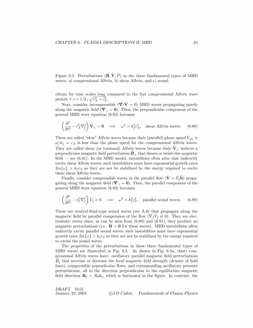
CHAPTER 6. PLASMA DESCRIPTIONS II: MHD 24
Figure 6.5: Perturbations (B, V, P ) in the three fundamental types of MHDwaves: a) compressional Alfven, b) shear Alfven, and c) sound.
obtain for time scales long compared to the fast compressional Alfven waveperiod: t >> 1/k⊥
√c2A + c2
S .Next, consider incompressible (∇·V = 0) MHD waves propagating purely
along the magnetic field (∇⊥ = 0). Then, the perpendicular component of thegeneral MHD wave equation (6.82) becomes(
∂2
∂t2− c2
A∇2‖
)V⊥ = 0 =⇒ ω2 = k2
‖c2A, shear Alfven waves. (6.88)
These are called “slow” Alfven waves because their (parallel) phase speed Vϕ‖ ≡ω/k‖ = cA is less than the phase speed for the compressional Alfven waves.They are called shear (or torsional) Alfven waves because their V⊥ induces aperpendicular magnetic field perturbation B⊥ that shears or twists the magneticfield — see (6.81). In the MHD model, instabilities often arise that indirectlyexcite shear Alfven waves; such instabilities must have exponential growth ratesImω > k‖cA so they are not be stabilized by the energy required to excitethese shear Alfven waves.
Finally, consider compressible waves in the parallel flow (V = V‖b) propa-gating along the magnetic field (∇⊥ = 0). Then, the parallel component of thegeneral MHD wave equation (6.82) becomes(
∂2
∂t2− c2
S∇2‖
)V‖ = 0 =⇒ ω2 = k2
‖c2S , parallel sound waves. (6.89)
These are neutral-fluid-type sound waves (see A.6) that propagate along themagnetic field by parallel compression of the flow (∇‖V‖ ,= 0). They are elec-trostatic waves since, as can be seen from (6.80) and (6.81), they produce nomagnetic perturbations (i.e., B = 0 for these waves). MHD instabilities oftenindirectly excite parallel sound waves; such instabilities must have exponentialgrowth rates Imω > k‖cS so they are not be stabilized by the energy requiredto excite the sound waves.
The properties of the perturbations in these three fundamental types ofMHD waves are illustrated in Fig. 6.5. As shown in Fig. 6.5a, (fast) com-pressional Alfven waves have: oscillatory parallel magnetic field perturbationsB‖ that increase or decrease the local magnetic field strength (density of fieldlines), compressible pependicular flows, and corresponding oscillatory pressureperturbations, all in the direction perpendicular to the equilibrium magneticfield direction B0 = B0ez, which is horizontal in the figure. In contrast, the
DRAFT 10:31January 28, 2003 c©J.D Callen, Fundamentals of Plasma Physics
CHAPTER 6. PLASMA DESCRIPTIONS II: MHD 25
(slow) shear Alfven waves (Fig. 6.5b) have: oscillatory perpendicular magneticfields B⊥ and oscillatory perpendicular flows V⊥ along the magnetic field, butno pressure perturbation (because these perurbed flows are incompressible). Fi-nally, as shown in Fig. 6.5c, the parallel sound waves have: no magnetic fieldperturbation (because they are electrostatic), an oscillatory compressible paral-lel flow V‖ and corresponding pressure P perturbations along the magnetic fielddirection.
In the more general case of propagation of MHD waves at arbitrary anglesto the magnetic field direction, these three types of waves become coupled (seeSection 7.6). These waves also become coupled in inhomogeneous magnetic fields— because the parallel and perpendicular directions vary spatially. Nonetheless,the basic wave characteristics we have discussed are usually still evident in thesemore complicated situations.
6.7 Magnetic Field Diffusion in MHD
In order to examine the effect of electrical resistivity on a plasma in the MHDmodel, consider first the evolution of the magnetic field in (6.71) without theadvection term:
∂B∂t
=η
µ0∇2B, magnetic field diffusion equation. (6.90)
This equation describes the diffusion (see Section A.5) of the magnetic field(both its magnitude and directional components) that is caused by the electricalresistivity of a plasma. The diffusion coefficient is
Dη =η
µ0=
meνe
µ0nee2$ 1.4 × 10³
(Zi
Te(eV)]3/2
) (lnΛ17
)m2/s
magnetic field diffusivity. (6.91)
Phenomenologically, since we can write Dη = νe(c/ωpe)2, magnetic field diffu-sion can be thought of [via D ∼ (∆x)2/∆t — see (??)] as emanating from arandom walk process in which magnetic field lines step a collisionless skin depth(∆x ∼ c/ωpe) in an electron collision time (∆t ∼ 1/νe). The relative magnitudeof the magnetic field diffusivity can be ascertained from its relationship to theclassical diffusivity D⊥ defined in (??):
D⊥η/µ0
=νe#2
e
νe(c/ωpe)2
(Te + Ti
2Te
)=
ne(Te + Ti)c2ε0B2
=β
2. (6.92)
Thus, for a plasma with β < 1 particles diffuse classically across magneticfield lines slower than the magnetic field lines themselves diffuse relative tothe plasma! However, in most plasmas of interest microscopic turbulence inplasmas causes an anomalous perpendicular transport that is rapid comparedto the magnetic field diffusion; hence one can usually consider the magnetic fieldto be stationary for calculations of anomalous transport.
DRAFT 10:31January 28, 2003 c©J.D Callen, Fundamentals of Plasma Physics

CHAPTER 6. PLASMA DESCRIPTIONS II: MHD 26
To illustrate the spatial and temporal scale lengths involved in magnetic diff-ision, consider the distance an electromagnetic wave can penetrate (see Section1.5) into a resistive medium in which the magnetic field behavior is governed by(6.90). For wavelike perturbations B ∼ exp[i(k·x − ωt)], the diffusion equationbecomes
−iωB = −k2(η/µ0)B =⇒ k =√
iωµ0/η = (1 + i)√
(ω/2)(µ0/η). (6.93)
To use the analysis of Section 1.5, we identify this complex wavenumber k asthe transmitted wavenumber kT in (??). Thus, an electromagnetic wave will bedissipated and damped exponentially, as it oscillates spatially (due to RekT )and propagates into a resistive medium, with a characteristic decay length of
δη ≡ 1Im(kT =
√2ω
η
µ0, resistive skin depth. (6.94)
It is called a “skin” depth because of its analogy with the problem of deter-mining how far an oscillating magnetic field (e.g., due to 60 Hz AC electricity)penetrates into a cylindrical wire of finite radius. This skin depth formula isappropriate for radian frequencies ω < νe, while the collisionless skin depth for-mula (??) is appropriate for higher frequencies — see Problem 6.25. For Te =2000 eV, which gives η/µ0 $ 0.016 m2/s (close to the resistivity of copper atroom temperature of η/µ0 $ 0.135 m2/s), the resistive skin depth ranges from0.07 mm for f = ω/2π = 104 Hz (ω = 2π × 104) to about 1 cm for 60 Hz.
Another way of illustrating the temporal behavior of magnetic field diffusionin a magnetized plasma is to ask: on what time scale τ will a magnetic fieldcomponent diffuse away from being localized to a region of width L⊥? Becausefor diffusive processes the diffusion coefficient scales with spatial and temporalsteps as D ∼ (∆x)2/∆t ∼ L2
⊥/τ (see Appendix A.5), we can estimate phe-nomenologically that τ ∼ L2
⊥/(η/µ0). One often considers a cylindrical modelconsisting of a column of magnetized plasma with radius a that initially carriesan axial current. For such a cylindrical model the resistivity-induced decay timeof the current (and induced azimuthal magnetic field) is (see Section A.5)
τη $ a2
6 η/µ0, resistive skin diffusion time. (6.95)
Here, the numerical factor of 6 is a cylindrical geometry factor which more pre-cisely is the square of the first zero of the J0 Bessel function: j2
0,0 $ 2.4052 $ 5.78— see Appendix A.5 and (??). However, the additional accuracy is unwarrantedboth because of the approximations involved in the simple model used to deriveτη and because of the intrinsic accuracy of the electrical resistivity ($ 1/ lnΛ ∼5–10%). For a plasma of radius a = 0.3 m with Te = 2000 eV, which givesη/µ0 $ 0.016 m2/s, the skin time is τη ∼ 1 s.
Finally, we discuss the relative importance of the two contributions to mag-netic field evolution (6.71) in the MHD model: advection of the magnetic fieldby ∇×(V×B), and resistive diffusion by (η/µ0)∇2B. The relative importance
DRAFT 10:31January 28, 2003 c©J.D Callen, Fundamentals of Plasma Physics
CHAPTER 6. PLASMA DESCRIPTIONS II: MHD 27
of these two terms is indicated by the scaling properties of their ratio:
S =|∇×(V×B)||(η/µ0)∇2B| ∼ cA/L‖
(η/µ0)/a2$ 1.6 × 10¹³ a2B[Te(eV)]3/2
L‖Zi√
niAi
(17
lnΛ
),
Lundquist number.4 (6.96)
Here, we have taken the typical velocity to be the Alfven speed cA and assumedscale lengths L‖ [e.g., periodicity scale length along B — see (6.81)] for theadvection process and a (e.g., plasma radius) for the magnetic diffusion. TypicalLundquist numbers range from 102 for cold, resistive plasmas, to 105–1010 forthe earth’s magnetosphere and magnetic fusion experiments, to 1010–1014 forthe sun’s corona and astrophysical plasmas.
Because the Lundquist number is large for almost all magnetized plasmasof interest (and extremely large for high temperature plasmas), one might betempted to just set the resistivity to zero (S → ∞) and always use the idealMHD model. Indeed, throughout most of a plasma the magnetic field is frozeninto and moves with the plasma fluid. However, a small resistivity can bevery important in resistive boundary layers. The boundary layers occur inthe vicinity of magnetic field lines where the parallel derivative (B0·∇)V⊥ in(6.81) vanishes so the B⊥ evolution becomes dominated by resistive evolutionof B⊥, rather than by advection. The width of these resistive boundary layersscales inversely with a fractional power of the Lundquist number (S−1/3 orS−2/5) and hence is not negligible — see Chapter 22. Since resistivity allows themagnetic field lines to slip relative to the plasma fluid, they relax (in the resistivelayers) the frozen flux constraint and thereby allow new types of instabilities— resistive MHD instabilities, which are described in Chapter 22. Since theresistivity only relaxes the frozen flux constraint in thin layers, resistive MHDinstabilities grow much slower (by factors of S−1/3 or S−3/5) than ideal MHDinstabilities. However, resistive MHD instabilities are quite important, becausethey can lead to turbulent plasma transport (see Section 25.3) and becausein these narrow resistive boundary layers the magnetic field lines can tear orreconnect and thereby lead to changes in the magnetic topology (see Section22.3). For example, they can nonlinearly evolve into a magnetic island structurelike that shown in Fig. 6.4c.
6.8 Which Plasma Description To Use When?
In this section we discuss which types of plasma descriptions are used for describ-ing various types of plasma processes in magnetized plasmas. This discussionalso serves as an introduction to most of the subjects that will be covered in theremainder of the book. The basic logic is that the fastest, finest scale processes
4Many plasma physics textbooks refer to this as the “magnetic Reynolds number.” How-ever, S is the ratio of linear advection to a dissipative process rather than the ratio of nonlinearadvection to a dissipative process, as the neutral fluid Reynolds number is — see (??). Wewill call S the Lundquist number to avoid the implication that this dimensionless number isindicative of nonlinear processes that always lead to turbulence when it is large.
DRAFT 10:31January 28, 2003 c©J.D Callen, Fundamentals of Plasma Physics
CHAPTER 6. PLASMA DESCRIPTIONS II: MHD 28
require kinetic descriptions, but then over longer time and length scales morefluidlike, macroscopic models become appropriate. Also, the “equilibrium” ofthe faster time scale processes often provide constraint conditions for the longertime scale, more macroscopic processes.
In a magnetized plasma there are many more relevant parameters, and theirrelative magnitudes and consequences can vary from one application to another.Thus, to provide a table similar to Table ?? for magnetized plasmas, we need tospecify the parameters for a particular application. We will choose parameterstoward the edge (r/a = 0.7) of a typical 1990s “large-scale” tokamak plasma(e.g., the Tokamak Fusion Test Reactor: TFTR): Te = Ti = 1 keV, ne = 3×10¹⁹
m−3, B = 4 T, deuterium ions, Zeff = 2, L‖ = R0q $ 6 m, a = 0.8 m, Lp = 0.5m. In a magnetized plasma the unmagnetized phenomena listed in Table ??still occur; however, their effects only influence responses along the magneticfield direction. Parameters for the gyromotion, bounce motion and drift motionof charged particles in this tokamak magnetic field structure are approximatelythe same as those indicated in (??) and (??).
Table 6.1 presents an outline of magnetized-plasma-specific plasma phenom-ena, and their relevant time scales, appropriate models and possible conse-quences for the tokamak plasma parameters indicated in the preceding para-graph. In it time scales are indicated in “half order of magnitudes” (100.5 =3.16 · · · ∼ 3). As indicated, the fastest magnetic-specific process in magnetizedplasmas is the gyromotion of particles about the magnetic field, for which the ap-propriate model is the Vlasov equation. The ion gyromotion leads to cyclotron(Bernstein) waves, finite ion gyroradius (FLR) effects and a perpendicular di-electric response (Sections 7.5, 7.6). There are of course also electron cyclotronmotion and waves. The propagation of (electron and ion) cyclotron-type wavesin plasmas and their use for wave heating of magnetized plasmas are discussedin Chapters 9 and 10. If the electron or ion distribution function is peaked at anonzero energy (so ∂f0/∂ε > 0), it can lead to cyclotron instabilities (Chapter18) whose nonlinear evolution to a steady state or bursting situation is oftendetermined by collisions (Section 24.1).
The next fastest time scales are typically those associated with the the Alfvenwave and sound wave frequencies which are described by the ideal MHD model:(6.25)–(6.39) with η → 0. As indicated in Table 6.1, in the usual situationwhere compressional Alfven waves are stable, their effect is to impose radial (⊥to B) force balance equilbrium [(6.48) and Chapter 20] on the plasma and lowerfrequency perturbations in the plasma. The shear Alfven and sound wavescan lead to virulent macroscopic current-driven (kink) and pressure-gradient-driven (interchange) instabilities (Chapter 21). The nonlinear consequencesof an ideal MHD instability is often dramatic movement or catastrophic lossof the plasma in a few to ten instability growth times; hence most magneticconfinement systems are designed to provide ideal MHD stability for the plasmasplaced in them.
Next, we turn to the sequentially slower particle and plasma motions along(‖), across (∧) and perpendicular (⊥) to the magnetic field B. The fastestmotion along a magnetic field line is the electron bounce motion, which is de-
DRAFT 10:31January 28, 2003 c©J.D Callen, Fundamentals of Plasma Physics

CHAPTER 6. PLASMA DESCRIPTIONS II: MHD 29
Table 6.1: Phenomena, Models For A Magnetized Plasma
Species,Physical Process Time Scales Plasma Model Consequences
cyclotron waves 1/ωci ∼ 10−8 s Vlasov dielectric resp.cyclotron inst. 1/ωci ∼ 10−8 s Vlasov NL, via collisions
Alfven waves ideal MHDcompressional a/cA ∼ 10−7 s ∇P = J×Bshear L‖/cA ∼ 10−6 s J-driven inst.
sound waves a/cS ∼ 10−5.5 s ideal MHD ∇P -driven inst.
parallel (‖) to B parallel kineticelectron bounce 1/ωbe∼10−6.5 s ‖ Vlasov ne, Te const. ‖Belectron collisions 1/νe ∼ 10−5 s drift kinetic η, q‖e, b ·∇· π‖e
ion bounce 1/ωbi∼10−4.5 s ‖ Vlasov ni, Ti const. ‖B
Ohm’s law in MHD >1/νe∼10−5 s resistive MHD resistive inst.
cross (∧) to Bdiamagnetic flow 1/ω∗ <∼ 10−5 s gyrokinetic drift wave inst.cross flow equil. 1/νi ∼ 10−3 s drift kinetic cross flow damp.
perp. (⊥) to Bplasma transport τE ∼ a2/4χ⊥ two-fluid loss of plasmaB field evolution τη ∼ a2µ0/6η res./neo. MHD B field diffusion,
magnetic islands
scribed by a parallel motion version of the Vlasov equation [the drift kineticequation (??) without the collision operator and drift velocity vD]. On timescales longer than the electron bounce time (1/ωbe), the lowest order distributionfunction becomes constant along field lines (∇‖f0e = 0 and hence density andtemperature become constant along B), and distinctions between trapped anduntrapped electrons and their differing particle orbits become evident. For theparameters chosen, we have an electron collision length λe = vTe/νe $ 200 m∼ 33L‖ and hence λe∇‖ ∼ 33 >> 1. This is a typical toroidal plasma which isoften (confusingly) called “collisionless” — because the collision length is longcompared to the parallel periodicity length. Since the electron gyroradius isnegligibly small, the collisional evolution of the electron species on the collisiontime scale (1/νe) is governed by the (electron) drift kinetic equation (??). Its so-lution for axisymmetric toroidal plasmas is discussed in Section 16.2*. For timeslong compared to the electron collision time the plasma acquires its electricalresistivity η and the collisions of untrapped electrons produce entropy through
DRAFT 10:31January 28, 2003 c©J.D Callen, Fundamentals of Plasma Physics

CHAPTER 6. PLASMA DESCRIPTIONS II: MHD 30
“neoclassical” heat conduction (q‖e) and parallel viscosity (b ·∇· π‖e) — seeChapter 16. Similarly, the lowest order ion distribution function, density andtemperature become constant along magnetic field lines for time scales longerthan the ion bounce time (1/ωbi) and their collisional effects (in relaxing crossflows within a magnetic flux surface) become evident on the ion collision timescale (1/νi).
The plasma exhibits an electrical resistivity for time scales longer than theelectron collision time (1/νe). Its introduction into MHD leads to the resistiveMHD model: (6.25)–(6.39). Since the introduction of resistivity relaxes theideal MHD frozen flux constraint (in narrow layers), it can lead to resistiveMHD instabilities related to their ideal MHD counterparts (kink → tearing,∇P -driven “interchange” → resistive interchange), which, however, grow moreslowly and hence are less virulent — see Chapter 22.
The next set of phenomena concern the effects of particle drifts and plasmaspecies flows in the cross direction (∧ — perpendicular to B and within a fluxsurface if it exists). On this time scale a global (as opposed to local) descriptionof the magnetic field is usually required. The diamagnetic flows of electronsand ions lead to drift-wave-type oscillations (Sections 7.4* and 8.6*) and insta-bilities (Section 23.3*). Since these “universal” instabilities involve modes withsignificant ion gyroradius (FLR) effects (#i∇⊥ ∼ k⊥#i ∼ 1), the gyrokineticequation is used to describe their nonlinear evolution into microsopic plasmaturbulence (Chapter 25) that leads to anomalous radial transport (Chapter 26)of the plasma. On the same time scales the combination of the E×B and dia-magnetic flows come into “equilibrium” (a steady state saturation or boundedcyclic behavior); flow components within a magnetic flux surface in directionsin which the magnetic field is inhomogeneous (e.g., the poloidal direction in anaxisymmetric tokamak) are damped on the ion collision time scale (1/νi) — seeSection 16.3*. Steady-state net radial transport fluxes can only be properly cal-culated after the flows within magnetic flux surfaces are determined and relaxedto their equilibium values. Also, in determining transport fluxes it is implicitlyassumed that nested magnetic flux surfaces exist and that “radial” transport isto be calculated relative to them.
Finally, we reach the transport time scales on which the plasma and mag-netic field diffuse radially out of the plasma confinement region, and radiation(Chapter 14) can be significant. Plasma transport (relative to the magneticfield) is usually modeled with two-fluid equations averaged over magnetic fluxsurfaces to yield equations that govern the transport of plasmas perpendicularto magnetic flux surfaces — see Chapter 17. However, the radial particle andheat diffusion coefficients D⊥, χ⊥ are usually assumed to be the sum of thoseproduced by anomalous transport (Chapter 26) and those due to classical [(??),(??) and Chapter 15] and neoclassical (Chapter 16) transport processes. For acylindrical-type plasma model the characteristic time scale for the usally dom-inant plasma energy loss is (see Section 17.3) approximately τE ∼ a2/4χ⊥ inwhich a is the plasma radius; for the plasma parameters we are considering itis of order 0.1 s. Simultaneously, the magnetic field is diffusing. The character-istic time scale for diffusive transport of magnetic field lines out of a cylindrical
DRAFT 10:31January 28, 2003 c©J.D Callen, Fundamentals of Plasma Physics
CHAPTER 6. PLASMA DESCRIPTIONS II: MHD 31
plasma is τη ∼ a2/(6η/µ0); for the plasma parameters we are considering it is oforder 1 s. If resistive or neoclassical MHD tearing-type instabilities are present,they can reconnect magnetic field lines on rational magnetic flux surfaces andevolve nonlinearly by forming magnetic islands which grow (to saturation ortotal plasma loss) on a fraction (∼ 0.1) of the magnetic field diffusion time scaleτη. Since the magnetic field typically diffuses more slowly than energy is lost viaanomalous transport (i.e., τη >> τE or η/µ0 << χ⊥), it is usually reasonableto assume that the magnetic field is stationary and the plasma moves relativeto it via Coulomb-collision-induced or anomalous plasma transport processes.
REFERENCES AND SUGGESTED READINGThe MHD description of a plasma and its properties are presented in
Schmidt, Physics of High Temperature Plasmas (1966,1979), Chapts. 3,4 [?]
Krall and Trivelpiece, Principles of Plasma Physics (1973), Chapts. 2.3 [?]
Freidberg, Ideal Magnetoydrodynamics (1987) [?]
Sturrock, Plasma Physics, An Introduction to the Theory of Astrophysical, Geo-physical & Laboratory Plasmas (1994), Chapts. 11,12 [?]
Hazeltine and Waelbroeck, The Framework of Plasma Physics (1998), Chapts.3–6 [?]
Bateman, MHD Instabilities (1980) [?]
Biskamp, Nonlinear Magnetohydodynamics (1993) [?]
The neoclassical MHD model for axisymmetric toroidal plasmas is described in
J.D. Callen, W.X. Qu, K.D. Siebert, B.A. Carreras, K.C. Shaing and D.A.Spong,“Neoclassical MHD Equations, Instabilities and Transport in Tokamaks,”in Plasma Physics and Controlled Nuclear Fusion Research 1986 (IAEA, Vienna,1987), Vol. II, p. 157 [?]
PROBLEMS
6.1 Use the definition of the pressure in (??) with vr ≡ v − V to show that theisotropic pressure of a species in the center-of-mass frame (V) of an MHD plasmais
pCMs = ps + (nsms/3)|Vs − V|2. /∗
6.2 Show that the plasma momentum equation (6.6) obtained by adding the electronand ion momentum equations is exact (i.e., it does not involve an me/mi << 1approximation). [Hint: To obtain the inertia term on the left it is easiest to use(??) for the electron and ion momentum equations. Also, first show that∑
s
msnsVsVs = ρmVV +∑
s
msns(Vs − V)(Vs − V)
in which V is the MHD mass flow velocity defined in (6.19).] //*
6.3 Evaluate ∇· JD and show that it is equal to ∇· J∗, and to the terms on theright of (6.16). Explain the physical significance of the equality of these twoquantities. //*
DRAFT 10:31January 28, 2003 c©J.D Callen, Fundamentals of Plasma Physics

CHAPTER 6. PLASMA DESCRIPTIONS II: MHD 32
6.4 Multiply the electron and ion momentum balance equations (??) by qe/me andqi/mi and add them to obtain the exact generalized Ohm’s law
∂J∂t
+ ∇· (JV + VJ − ρqVV) = ε0ω2p
E + V×B −
(J‖σ‖
+J⊥σ⊥
)− (1 − Zime/mi)J×B − ∇· [PCM
e − Zi(me/mi)PCMi ]
(1 + Zime/mi)nee
in which PCM
s ≡ psI + πs + nsms(Vs − V)(Vs − V) is the pressure tensor ofa species in the center-of-mass frame (V) of the plasma. Show that this resultsimplifies to (6.17) for me/mi << 1 and strongly subsonic relative species flows(|Vs −V|/vTs << 1). [Hint: Use ne/ni = qi/e = Zi for this two species plasmaand
Ve = V − mini(J/nee)
mene + mini, Vi = V +
mene(J/nee)
mene + mini.] ///∗
6.5 Show that the electron inertia term is negligible compared to the electric fieldin the parallel generalized Ohm’s law for kc/ωpe << 1. [Hint: Use the parallelcomponent of the nonrelativistic Ampere’s law: ∇2A‖ = −µ0J‖ from (??).] //*
6.6 Show that for a wavelike perturbation in a sheared slab model magnetic fieldthe perturbed electron pressure gradient is negligible in the parallel generalizedOhm’s law when (6.19) is satisfied and ω >> ω∗e. [Hint: When the magneticfield is perturbed in MHD B → B0 + ∇×A & B0 + ∇A‖×b and ∇‖ ≡ b ·∇is changed accordingly.] //*
6.7 Show that the perpendicular electron inertia term is a factor of at least ω/ωce
smaller than E⊥ in (6.20) and hence negligible in MHD. [Hint: Show that for thediamagnetic and polarization MHD currents the electron inertia term is smallerthan that due to the electron polarization flow (??).] //*
6.8 Derive the MHD system momentum density equation (6.35). [Hint: Rewrite themomentum equation (6.27) using Ampere’s law and vector identities (??), (??)and (??).] //
6.9 Derive the MHD system energy density equation (6.36). [Hint: Take the dotproduct of V with the MHD momemtum equation (6.45), and simplify the resultusing Ohm’s law in the form V×B = ηJ − E, vector identities (??) and (??),and
V·∇P =1
Γ− 1∂P∂t
+Γ
Γ− 1∇·PV − ηJ2,
which is obtained from a combination of the equation of state (6.29) and themass density equation (6.25).] //
6.10 Use the tensor form of Gauss’ theorem (??) to calculate the force on a volumeof MHD fluid in terms of a surface integral over the stress tensor. Use aninfinitesimal volume form of your result to discuss the components of the forcein the ex, ey, b directions. //
6.11 The pressure tensor in an open-ended magnetic mirror is anisotropic becauseof the loss-cone. a) Show that for species distribution functions fs which donot depend on the gyroangle ϕ the pressure tensor is in general of the formP = P⊥(I − bb) + P‖bb in which P⊥ = P⊥(α,β, B) and P‖ = P‖(α,β, B). b)
DRAFT 10:31January 28, 2003 c©J.D Callen, Fundamentals of Plasma Physics
CHAPTER 6. PLASMA DESCRIPTIONS II: MHD 33
Work out ∇· P. c) Show that the condition for force balance along a magneticfield (b ·∇· P = 0) can be reduced to
∂P‖∂B
∣∣∣∣α,β
=P‖ − P⊥
B.
d) Discuss how this result indicates confinement of plasma along the magneticfield in a magnetic mirror. ///
6.12 Obtain the angle between J and B in a screw pinch equilibrium as a functionof a relevant plasma β. //*
6.13 Consider a pressure profile given by P (x)/P (0) = exp(−x2/a2) in a sheared slabmagnetic field model with no curvature or shear. a) Calculate the diamagneticcurrent. b) Determine the Bz(x) profile induced by this diamagnetic current.c) Show that the plasma pressure produces a diamagnetic effect. d) Show thatyour Bz(x) agrees with (6.59). //
6.14 Consider the MHD radial force balance equilibrium of a cylindrical plasma witha pressure profile P (r) that vanishes for r ≥ a which is placed in a uniformmagnetic field B = B0ez. Use the azimuthal component of Ampere’s law for Jθ
and solve the resultant force balance equation for Bz(r). Show that your resultagrees with (6.59). /
6.15 One definition of a magnetic field line is d#×B = 0. Show that its time deriva-tive yields the magnetic evolution equation (6.71). How does this show that amagnetic field line is advected with the moving plasma in the ideal MHD limit?[Hint: Use vector identities (??) for (d/dt)d# and (??), (??).] //
6.16 Show that for a Clebsch magnetic field representation B = ∇α×∇β the idealMHD evolution equation (6.71) is satisfied by dα/dt = dβ/dt = 0. Why doesthis show that a magnetic field line is advected with an ideal MHD plasma? //
6.17 Derive the canonical flux invariant for an isentropic plasma species that is acombination of the magnetic flux and species vorticity flux which is deducedfrom the canonical momentum (??) ps = msv + qsA as follows. a) First,average the canonical momentum over a Maxwellian distribution to obtain ps =msVs + qsA. b) Next, use this result to define a species canonical flux invariant
ψ#s ≡∫∫
S
dS ·∇×(
A +ms
qsVs
)=
∫∫S
dS ·(
B +ms
qs∇×Vs
).
c) Obtain dψ#s/dt and use the species momentum equation (??) to show that
dψ#s
dt= −
∫∫S
dS ·∇×(∇ps + ∇· πs − Rs
nsqs
).
d) Show that dψ#s/dt = 0 for an isentropic plasma species. e) Discuss how thecanonical flux invariant ψ#s combines the ideal MHD frozen flux theorem (6.73)and the Kelvin circulation theorem (??). f) Indicate the physical processesthat can cause net transport of a plasma species relative to the canonical fluxsurfaces ψ#s. g) Why doesn’t inertia contribute to transport relative to the ψ#s
surfaces? [Hint: Use vector identities (??), (??) and (??) in part c).] ///*
DRAFT 10:31January 28, 2003 c©J.D Callen, Fundamentals of Plasma Physics

CHAPTER 6. PLASMA DESCRIPTIONS II: MHD 34
6.18 Show that for the MHD model the electron and ion canonical fluxes defined inthe preceding problem are, to lowest order in (me/mi)
1/2 << 1,
ψ#e &∫∫
S
dS ·(
1 − c2
ω2pe
∇2
)B, ψ#i &
∫∫S
dS ·(
B + Bcωpi
∇× VcA
).
Use these two relations to discuss the degree to which the magnetic field is frozeninto the electron and ion fluids in an ideal MHD plasma. //*
6.19 Show that the total mass M of an MHD plasma in a volume V that moves withthe plasma flow velocity V will be conserved if the mass density satisfies themass density equation (6.25). [Hint: Determine the condition for dM/dt = 0and use vector identity (??) for (d/dt)d3x.] //
6.20 Work out the terms on the right of (6.82). [Hint: Since B = B0b is spatiallyuniform, it commutes with the ∇‖ ≡ b ·∇ and ∇⊥ = ∇ − b∇‖ operators.] //
6.21 Work out formulas for the ratio of the electron and ion thermal speeds to theAlfven speed in terms of βe ≡ 2µ0pe/B2 and βi ≡ 2µ0pi/B2. What are theseratios for a β = 0.08, Te = Ti, electron-deuteron plasma? /
6.22 How large would the magnetic field strength B have to be for the Alfven speedto be equal to the speed of light for ne = 1020 m−3 and Ai = 2? /
6.23 Show that for perturbations on the equilibrium time scale for compressionalAlfven waves
B‖/B0 = − (β/2) (P /P0). /
6.24 Since to lowest order in me/mi << 1 the MHD momentum equation results fromthe ion momentum equation, on the equilibrium time scale for compressionalAlfven waves the radial component of the ion momentum equation should be inequilibrium. Show that the equilibrium radial ion momentum (force) balanceequation in a screw pinch plasma yields the following relation for the axial flowin terms of the radial electric field, pressure gradient and poloidal flow:
Viz = − 1Bθ
(dΦ0
dr+
1n0iqi
dp0i
dr− ViθBz
). /∗
6.25 Determine the frequency ranges where an electromagnetic wave impinging onan unmagnetized plasma: a) propagates through it, b) is evanescent on a c/ωpe
length scale, and c) dissipatively decays in a resistive skin depth (6.94)? [Hint:review Section 1.5 and consider a time-dependent electrical conductivity.] //
6.26 Show that the Lundquist number can be written in terms of fundamental mi-croscopic variables as
S =ωce
νe
ac/ωpi
aL‖
Should S always be a large number for a magnetized MHD plasma? /
DRAFT 10:31January 28, 2003 c©J.D Callen, Fundamentals of Plasma Physics

APPENDIX A. PHYSICS EQUATIONS, UNITS, AND CONSTANTS 1
Appendix A
Physics Equations, Units,and Constants
This appendix provides a summary of the fundamental physical laws from otherareas of physics, as they are commonly used in plasma physics. Key equations,units and physical constants are given for mechanics, electrodynamics, statisticalmechanics, kinetic theory of gases, stochastic diffusion processes, fluid mechan-ics and quantum mechanical effects. While the procedures for deriving theseequations are given in outline form, details are omitted. Readers should con-sult the textbook references listed at the end of each section for more detailedexplanations and theoretical developments. In some parts of this appendixextensive use is made of the vector algebra and calculus relations given in Ap-pendix D. The International System of Units (Systeme International d’Unites),often called mks units, are used throughout this appendix, and the book. Phys-ical constants and SI unit interrelationships are given in tables in Section A.8at the end of this Appendix.
A.1 Mechanics
Newton’s second law states that the mass m times the acceleration a of a particleis given by the force F (in units of newtons or kg ·m/s2)
ma = F, Newton’s second law. (A.1)
A conservative force is one that is derivable from the gradient of a potentialthat is independent of time:
F = −∇V (x), conservative force. (A.2)
Since the acceleration in (A.1) is just the time derivative of the particle velocity,a ≡ dv/dt, taking the dot product of the velocity v with Newton’s second law
DRAFT 11:16September 2, 2003 c©J.D Callen, Fundamentals of Plasma Physics

APPENDIX A. PHYSICS EQUATIONS, UNITS, AND CONSTANTS 2
for a conservative force yields:
d
dt
[mv2
2+ V (x)
]= 0 =⇒ ε =
mv2
2+ V (x) = constant,
energy conservation, (A.3)
where mv2/2 ≡ m(v · v)/2 ≡ T is the particle kinetic energy and V (x) is thepotential energy. The SI unit of energy is the joule (J), which is equal to anewton ·meter (N ·m). In plasma physics particle energies are usually quotedin electron volts (eV), which is the energy in joules divided by the elementarycharge [ eV ≡ J/e = J/(1.602 × 10−19) ].
The force on a particle of charge q subjected to an electric field E(x, t) anda magnetic induction field B(x, t) is
F = q (E + v×B) , Lorentz force. (A.4)
For electrostatic situations with no magnetic field, the electric field can be writ-ten in terms of the electrostatic potential φ(x) : E = −∇φ. Then, the Lorentzforce becomes conservative [see (A.2)] with V (x) = −qφ(x), and the energyconservation relation (A.3) is applicable.
When only a magnetic field is present, the combination of Newton’s secondlaw and the Lorentz force becomes
mdvdt
= qv×B =⇒ dvdt
= ωc×v, (A.5)
where
ωc ≡ − qB/m, the angular velocity, (A.6)
for gyromotion of the charged particle in the magnetic field. The negative signis needed in this vectorial definition so that charged particles gyrate accordingto the right-hand rule with the thumb pointing in the direction of ωc. Themagnitude of ωc gives the radian frequency (rad/s) for the gyromotion:
ωc = qB/m, gyrofrequency, (A.7)
which is also called the cyclotron (the source of the subscript c) or Larmor1frequency. This formula is unchanged for relativistic particles except for thefact that then the mass becomes the relativistic mass: m → m/
√1 − v2/c2.
Since the dot product of (A.5) with the velocity v vanishes, the particle kineticenergy is constant — a magnetic field does no work on a charged particle in itsgyromotion. In gyromotion a charged particle executes a circular motion aboutthe magnetic field B with a radius of
# ≡ v⊥/ωc, gyroradius, (A.8)
in which v⊥ is the magnitude of the velocity component perpendicular to themagnetic field direction [v⊥ ≡ −B×(B×v)/B2].
1Actually, the Larmor frequency is defined to be half the cyclotron frequency.
DRAFT 11:16September 2, 2003 c©J.D Callen, Fundamentals of Plasma Physics

APPENDIX A. PHYSICS EQUATIONS, UNITS, AND CONSTANTS 3
For situations where both electric and magnetic fields are present, it is conve-nient to write them in terms of the scalar potential φ(x, t) and vector potentialA(x, t): E = −∇φ−∂A/∂t, B = ∇×A — see (A.55). Then, Newton’s secondlaw (A.1) for a nonrelativistic charged particle subjected to the Lorentz force(A.4) can be written as
mdvdt
= − ∂U∂x
+d
dt
(∂U
∂v
), U = qφ− q(v · A) (A.9)
in which U is a generalized potential energy, ∂U/∂x ≡ ∇U , ∂U/∂v ≡ ∇vU ,where ∇v is the gradient in velocity space. The single particle Lagrangian, whichhas units of energy and is given by the kinetic energy minus the generalizedpotential energy, is defined by
L(x,v, t) ≡ T − U =mv2
2− qφ+ q(v · A), Lagrangian, (A.10)
where again T = mv2/2 is the particle kinetic energy. The vector equation ofmotion for a charged particle (i.e., Newton’s second law with the Lorentz force)can be written in terms of the Lagrangian as
d
dt
(∂L
∂v
∣∣∣∣t,x
)− ∂L
∂x
∣∣∣∣t,v
= 0, Lagrangian equations of motion. (A.11)
For an orthogonal coordinate system with unit base vectors ek, the orthogonalprojections of this vector equation yield
d
dt
(∂L
∂qk
)− ∂L
∂qk= 0, k = 1, 2, 3 Lagrange’s equations. (A.12)
Here, the spatial coordinates are qk ≡ ek · x and the velocity coordinates areqk ≡ ek · v = ek · dx/dt. Note that, like Newton’s second law, Lagrange’sequations are in general second order ordinary differential equations in time.
It is often convenient to change the charged particle equation of motion intotwo coupled first order differential equations. To effect this change one firstdefines
p ≡ ∂L
∂v= mv + qA, canonical momentum, (A.13)
in which v ≡ dq/dt. Next, the single particle Hamiltonian function H, whichalso has units of energy, is defined through the Legendre transformation:
H(x,p, t) ≡ p · dxdt
− L =|p − qA|2
2m+ qφ ≡ T + V, Hamiltonian. (A.14)
It is the sum of the kinetic energy (T = |p − qA|2/2m = mv2/2) and thepotential energy (V = qφ), and by construction is independent of velocity:∂H/∂v|x,p,t = 0. The equation of motion for a charged particle can be written
DRAFT 11:16September 2, 2003 c©J.D Callen, Fundamentals of Plasma Physics
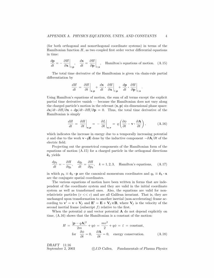
APPENDIX A. PHYSICS EQUATIONS, UNITS, AND CONSTANTS 4
(for both orthogonal and nonorthogonal coordinate systems) in terms of theHamiltonian function H, as two coupled first order vector differential equationsin time:
dpdt
= − ∂H
∂x
∣∣∣∣t,p
,dxdt
=∂H
∂p
∣∣∣∣t,x
, Hamilton’s equations of motion. (A.15)
The total time derivative of the Hamiltonian is given via chain-rule partialdifferentiation by
dH
dt=∂H
∂t
∣∣∣∣x,p
+dxdt
· ∂H∂x
∣∣∣∣t,p
+dpdt
· ∂H∂p
∣∣∣∣t,x
.
Using Hamilton’s equations of motion, the sum of all terms except the explicitpartial time derivative vanish — because the Hamiltonian does not vary alongthe charged particle’s motion in the relevant (x,p) six-dimensional phase space:dx/dt · ∂H/∂x + dp/dt · ∂H/∂p = 0. Thus, the total time derivative of theHamiltonian is simply
dH
dt=∂H
∂t
∣∣∣∣x,p
= − ∂L
∂t
∣∣∣∣x,v
= q
(∂φ
∂t− v · ∂A
∂t
), (A.16)
which indicates the increase in energy due to a temporally increasing potentialφ and due to the work v · qE done by the inductive component −∂A/∂t of theelectric field.
Projecting out the geometrical components of the Hamiltonian form of theequations of motion (A.15) for a charged particle in the orthogonal directionsek yields
dpk
dt= − ∂H
∂qk,
dqk
dt=∂H
∂pk, k = 1, 2, 3, Hamilton’s equations, (A.17)
in which pk ≡ ek · p are the canonical momentum coordinates and qk ≡ ek · xare the conjugate spatial coordinates.
The various equations of motion have been written in forms that are inde-pendent of the coordinate system and they are valid in the initial coordinatesystem as well as transformed ones. Also, the equations are valid for non-relativistic particles (v << c) and are all Galilean invariant. That is, they areunchanged upon transformation to another inertial (non-accelerating) frame ac-cording to v′ = v + Vf and E′ = E + Vf×B, where Vf is the velocity of thesecond inertial frame (subscript f) relative to the first.
When the potential φ and vector potential A do not depend explicitly ontime, (A.16) shows that the Hamiltonian is a constant of the motion:
H =|p − qA|2
2m+ qφ =
mv2
2+ qφ = ε = constant,
for∂φ
∂t= 0,
∂A∂t
= 0, energy conservation. (A.18)
DRAFT 11:16September 2, 2003 c©J.D Callen, Fundamentals of Plasma Physics

APPENDIX A. PHYSICS EQUATIONS, UNITS, AND CONSTANTS 5
In such conservative systems the particle energy and time are canonical conju-gate Hamiltonian coordinates: p = ε and q = t.
When the gradient of the Hamiltonian vanishes in a particular direction ek,(A.15) shows that the conjugate canonical momentum in the same direction isa constant of the motion:
pk ≡ ek · p = ek · (mv + qA) = constant for ek · ∂H∂x
= 0,
canonical momentum conservation. (A.19)
In an orthogonal coordinate system the base vector ek becomes the unit vectorek; then, the criterion for canonical momentum conservation in the ek directionbecomes simply ∂H/∂qk = 0 (i.e., H independent of the coordinate qk, whichimplies symmetry in the ek direction).
Lagrange’s or Hamilton’s equations of motion can be derived (by consideringvariations with x and v ≡ dx/dt or p as the independent variables, respectively)from Hamilton’s variational principle of least action (time integral of differencebetween kinetic and potential energy): δ
∫L dt = 0. It can also be shown using
(A.14) that for a conservative system where the Hamiltonian is a constant of themotion [see (A.18)], the action
∫p · dq is a variational quantity along a particle
trajectory.For periodic motion in a given coordinate qi it is convenient to introduce as
a variable the action integral over a cycle:
Ji =12π
∮pi · dqi =
12π
∫ 2π
0dθi pi · ∂qi
∂θi, action variable. (A.20)
The action variable, which is a momentum-like quantity, is the “area” in pi, qi
phase space encompassed by the periodic motion. The canonically conjugateaction-angle θi is the angular or cyclic variable corresponding to periodic motionaround the perimeter of this area. Hamilton-Jacobi theory (see references at endof this section) can usually be used to determine the action angle coordinateqi ≡ θi. Writing the Hamiltonian in terms of the action variable Ji, the Hamiltonequation dqi/dt = ∂H/∂pi [see (A.17)] becomes:
dθidt
=∂H
∂Ji≡ ωi, action angle evolution equation. (A.21)
The period of the oscillatory motion can be determined in general from
τi ≡∮
dt =∮
dqi
dqi/dt=∮
dqi
∂H/∂pi, oscillation period. (A.22)
The radian frequency for the periodic motion is
ωi(Ji) = 2π/τi, oscillation frequency. (A.23)
The Hamiltonian for a periodic system in action-angle variables is thus simply
Hi = ωiJi, action-angle Hamiltonian. (A.24)
DRAFT 11:16September 2, 2003 c©J.D Callen, Fundamentals of Plasma Physics

APPENDIX A. PHYSICS EQUATIONS, UNITS, AND CONSTANTS 6
For nearly periodic motion in situations where the generalized potential Uin (A.9) varies slowly and aperiodically in space and time (compared to theoscillations), the action in (A.20) is nearly constant and given by the ratio ofthe oscillation energy to the oscillation frequency:
Ji ' Hi
ωi=
εi
ωi, action for nearly periodic motion. (A.25)
For slow, temporal changes that are characterized by a parameter a(t) and arenot themselves periodic, it can be shown that, while the slow variations cause“linearly small,” oscillatory [∼ (a/ωia) sinωit << 1] changes in J , the averageof dJ/dt over an oscillation period τ is “quadratically small” in the rate oftemporal change:⟨
dJi
dt
⟩θi
≡ 1τ
∮dθi
θi
dJi
dt= 0 + O
(a
ωia
)2
,a
ω2i a
Ji
τ, (A.26)
where the dots over quantities indicate their time derivatives. For such situ-ations the action Ji is called an adiabatic invariant; it is often a very usefulapproximate constant of the motion. When the small variations in the poten-tial oscillate at a slow frequency ωi >> ωa ≡ √−(1/a) ∂2a/∂t2, harmonics ofthis slower oscillation that are resonant with the fundamental oscillations (i.e.,ωi = nωa, n ≡ an integer) can lead to secular changes in the action Ji that growslowly in time. Hence they can break the constancy of the adiabatic invariantover a long time period. This usually occurs when the slow oscillations exceed asmall critical amplitude (typically ∼ 0.1 of the main oscillations). The relevantmultiple time scale analysis and conditions for such breakdowns of adiabaticityare discussed in E.6.
As an example of the use of mechanics theory, consider the “central-force”problem of determining the scattering angle ϑ and elastic cross-section σ for aCoulomb collision of two non-relativistic, charged particles. Assume a chargedparticle of species s with charge qs, mass ms and initial velocity v experiences aCoulomb collision (i.e., interaction via the Coulomb electric field force) with an-other charged particle of species s′ with parameters qs′ , ms′ and v′. Multiplyingthe force balance equations obtained from (A.1) and (A.4) for each particle bythe mass of the other particle and subtracting, taking account of the equal andoppositely directed electric field forces on the two particles due to the Coulombpotential [qE = −q∇φ, φ = q/(4πε0|x|) — see (A.33)], yields the equationof motion for the two-particle system in the center-of-momentum coordinatesystem:
mss′d
dt(v − v′) = − qsqs′
4πε0∇ 1|x − x′| (A.27)
in which mss′ = msms′/(ms + ms′) is the “reduced” mass for the two particlesystem.
Initially, when the particles are very far apart, one can define the impactspeed as u = |v−v′| and the collision impact parameter as b (distance of closest
DRAFT 11:16September 2, 2003 c©J.D Callen, Fundamentals of Plasma Physics
APPENDIX A. PHYSICS EQUATIONS, UNITS, AND CONSTANTS 7
approach if the Coulomb electric field did not deflect the particles). Further,one defines the classical (i.e., not quantum mechanical) minimum distance ofclosest approach as
bclmin ≡ qsqs′
4πε0mss′u2, classical minimum impact parameter (A.28)
at which the center-of-momentum kinetic energy is half the Coulomb potentialenergy [qsqs′/(4πε0bcl
min)] and below which large-angle deflections (> 90) canbe expected to occur.
Since the collision takes place in a plane defined by the vectors x − x′ andv − v′, it is convenient to define instantaneous radial and angular coordinatesin the center-of-momentum frame by the radial separation of the particles r ≡|x − x′| and by the angle θ that the line x − x′ makes with the line |x − x′|when the particles were initially very far apart. In these coordinates the angularmomentum pθ [constant because of symmetry of the Coulomb potential in theθ direction — see (A.19)] and total energy ε [constant because the potential φdoes not depend explicitly on time — see (A.18)] can be written as
pθ = mss′r2θ = mss′bu,
ε = T + V =12mss′
(r2 + r2θ2
)+
qsqs′
4πε0r =12mss′u2.
Solving the second (energy conservation) equation for r and dividing by the θobtained from the first equation yields
dr
dθ= ±r
b
√r2 − 2 r bcl
min − b2,
where the sign is negative when the particles are approaching each other andpositive as they recede.
At the minimum or closest approach distance rm, dr/dθ = 0. The angle θmat this point is given by
θm =∫ ∞
rm
dr
dr/dθ= − arctan
(bclmin
b
)+π
2.
In the center-of-momentum frame the angular deflection ϑ caused by the colli-sion is given by π − 2θm and hence
tanϑ
2=
bclmin
b=
qsqs′
4πε0mss′u2b, scattering angle. (A.29)
Thus, b > bclmin causes Coulomb scattering by less than 90 (ϑ < π/2), while
b < bclmin induces more than 90 scattering.
The differential cross-section dσ (measured in meters2 or barns ≡ 10−28 m2)by which Coulomb collisions of incoming charged particles of species s withimpact parameter b and azimuthal angle ϕ scatter off of charged particles of
DRAFT 11:16September 2, 2003 c©J.D Callen, Fundamentals of Plasma Physics
APPENDIX A. PHYSICS EQUATIONS, UNITS, AND CONSTANTS 8
species s′ into spherical angles ϑ,ϕ within the differential solid angle dΩ ≡sinϑ dϑ dϕ is thus given [using (A.29) to write b(ϑ) = bcl
min/ tan(ϑ/2)] by
dσ = b db dϕ =b
sinϑ
∣∣∣∣ db
dϑ
∣∣∣∣ dΩ =(
bclmin
2 sin2 ϑ/2
)2
dΩ
or,
dσ
dΩ=(
bclmin
2 sin2 ϑ/2
)2
=(
qsqs′
24πε0mss′u2 sin2 ϑ/2
)2
,
Rutherford differential scattering cross-section. (A.30)
Standard intermediate level mechanics textbooks, which include extensionsto relativistic systems, are:
Symon, Mechanics (1971) [?].
Barger and Olsson, Classical Mechanics: A Modern Perspective (1973) [?].
The standard advanced level mechanics textbook is:Goldstein, Classical Mechanics (1950, 1980) [?].
A.2 Electrodynamics
An electrostatic theory is appropriate for time-independent charge density distri-butions ρq(x), electric fields E(x), and magnetic induction fields B(x). In elec-trostatics the irrotational (∇×E = 0) electric field E with units of volts/meteris written in terms of the scalar potential φ(x) with units of volts, E ≡ −∇φ,and related to the charge density distribution:
∇· E = ρq/ε0, Gauss’ law, (A.31)
−∇2φ = ρq/ε0, Poisson’s equation. (A.32)
The charge density distribution has units of coulombs/meter3. For localizedcharge density distributions [lim|x|→∞ ρq(x) → 0] the general (Green-function-type) solution of Poisson’s equation in an infinite medium is [see also (??)]
φ(x) =∫
d3x′ ρq(x′)4πε0 |x′ − x| . (A.33)
For a point charge at x = x0 the charge distribution is ρq(x) = q δ(x− x0) andthe potential becomes
φ(x) =q
4πε0 |x − x0| , Coulomb potential. (A.34)
Here and throughout this book the mks factor 4πε0 is written in braces;eliminating this factor yields the corresponding cgs forms of these electrostaticresponse formulas.
DRAFT 11:16September 2, 2003 c©J.D Callen, Fundamentals of Plasma Physics

APPENDIX A. PHYSICS EQUATIONS, UNITS, AND CONSTANTS 9
In a dielectric (ponderable) medium the charge density ρq is composed of apart ρfree due to “free” charges and a part due to a polarization charge density,ρpol = −∇· P where P ≡ ε0χEE is the presumed linear and isotropic polariza-tion (units of coulomb/meter2) of the medium induced by the electric field Eand χE is the dimensionless electric susceptibility of the medium:
ρq = ρfree + ρpol = ρfree − ∇· P = ρfree − ∇· ε0χEE. (A.35)
Thus, in an isotropic dielectric medium Gauss’ law becomes Coulomb’s law:
∇· D = ρfree, D ≡ ε0E + P = ε0(1 + χE)E = εE (A.36)
in which the medium’s dielectric constant ε ≡ ε0(1 + χE) is the constituitiverelation between the displacement vector D and the electric field E.
A magnetostatic theory is appropriate for time-independent current densitydistributions J(x) and magnetic induction fields B(x). In magnetostatics thesolenoidal (transverse, ∇· B = 0) magnetic induction field B which has unitsof weber/meter2 or tesla can be written in terms of the vector potential A, i.e.,B = ∇×A, and related to the current density distribution J which has unitsof ampere/meter2:
∇×B = µ0J =⇒ −∇2A = µ0J, static Ampere’s law (A.37)
in which ∇·A = 0 (the Coulomb gauge) has been assumed in the last form. Forlocalized current density distributions [lim|x|→∞ J(x) = 0], the general (Green-function-type) solution for A in an infinite medium is [see also (??)]
A(x) =µ0
4π
∫d3x′ J(x′)
|x′ − x| . (A.38)
The magnetic field around an infinite wire carrying a current I (amperes) alongthe z axis of a cylindrical coordinate system can obtained from this equationusing B = ∇×A and a current density J = ez(I/2πr) lima→0 δ(r − a):
B =µ0I
2πreθ, magnetic field around a current-carrying wire. (A.39)
To obtain the corresponding cgs form of this and other magnetic field responseequations, eliminate the µ0/4π factor and replace J by J/c, or replace µ0Jby 4πJ/c.
In a magnetizable medium the current density J is composed of a part Jfree
due to the current induced by “free” charges and a magnetization current den-sity Jmag = ∇×M where M ≡ χMH is the presumed linear and isotropicmagnetization (units of ampere-turns/meter) of the medium induced by themagnetic field H (units of ampere-turns/meter) and χM is the dimensionlessmagnetic susceptibility of the medium:
J = Jfree + Jmag = Jfree + ∇×M = Jfree + ∇×(χMH). (A.40)
DRAFT 11:16September 2, 2003 c©J.D Callen, Fundamentals of Plasma Physics

APPENDIX A. PHYSICS EQUATIONS, UNITS, AND CONSTANTS 10
Thus, in an isotropic, magnetizable medium the static Ampere’s law becomes
∇×H = µ0J, H = B/µ0 − M, B = µ0(1 + χM )H = µH (A.41)
in which µ = µ0(1 + χM ) is the magnetic permeability of the medium andB = µH is the constituitive relation between the magnetic induction B and themagnetic field H.
The microscopic Maxwell or electromagnetic (em) equations for determiningtime-varying electric and magnetic fields caused by charge and current densitydistributions ρq(x, t) and J(x, t), respectively, in free space are
Maxwell Equations
name
differential form integral form
Gauss’ law
∇· E =ρq
ε0
∫©∫
SdS · E =
∫V
d3xρq
ε0(A.41a)
Faraday’s law
∇×E = − ∂B∂t
∮C
d" · E = − ∂
∂t
∫∫S
dS · B (A.41b)
no magnetic monopoles
∇· B = 0∫©∫
SdS · B = 0 (A.41c)
Ampere’s law
∇×B = µ0
(J + ε0
∂E∂t
) ∮C
d" · B = µ0
∫∫S
dS ·(J + ε0
∂E∂t
)(A.41d)
(A.42)
Here, ε0 is the electric permittivity of free space which has units of farad/meter= coulomb/(volt ·meter) = joule/(volt2·meter), µ0 is the magnetic permeabil-ity of free space which has units of henry/meter = weber/(ampere ·meter) =weber2/(joule ·meter) and µ0ε0 = 1/c2 where c is the speed of light in free space.Taking the divergence of Ampere’s law and making use of Gauss’ law yields
∂ρq
∂t+ ∇· J = 0, continuity equation for charge and current. (A.43)
In Ampere’s law the displacement current ε0∂E/∂t was introduced by Maxwellto make the electrodynamics equations consistent with the charge and currentcontinuity equation (A.43).
DRAFT 11:16September 2, 2003 c©J.D Callen, Fundamentals of Plasma Physics

APPENDIX A. PHYSICS EQUATIONS, UNITS, AND CONSTANTS 11
The physical significance of the source terms on the right of the integralforms of the Maxwell equations are:
∫V d3x ρq ≡ Q, net charge (in coulombs)
within the volume V ;∫∫
S dS · B ≡ ψ, magnetic flux (in webers) penetratingthe surface S;
∫∫S dS · J ≡ I, the total electric current (in amperes) flowing
through the surface S. The Maxwell equations are relativistically invariant; inparticular, they are invariant under Lorentz transformations, which preserve theconstancy of the speed of light, independent of the motion of the source, upontransformation to another inertial rest frame.
The corresponding macroscopic Maxwell equations in an isotropic, polariz-able, magnetizable medium are written in terms of D ≡ εE = ε0E + P and themagnetic field H ≡ B/µ0 − M, and free charge, current densities ρfree,Jfree:
∇· D = ρfree, ∇×E = − ∂B/∂t, ∇ · B = 0, ∇×H = Jfree + ∂D/∂t.(A.44)
The total rate at which the electromagnetic (em) fields do work on a mediumin a finite volume V is
∫V d3x Jfree· E — the magnetic field does no work since
the magnetic force qv×B on charged particles is perpendicular to the velocity.Using the macroscopic Maxwell equations to calculate the rate of doing workyields the energy conservation law for electromagnetic fields:
∂wem
∂t+ ∇· Sem = −Jfree· E, em field energy conservation, (A.45)
where
wem ≡ wE + wB ≡ 12
(E · D + B · H), em energy density (J/m3), (A.46)
Sem = E×H, Poynting vector (flux of em energy) (J/m2· s), (A.47)
Jfree· E = joule heating (W/m3 = J/m3· s = V·A/m3), (A.48)
in which the energy densities in the electric and magnetic fields are defined by
wE ≡ 12
(E · D), electric field energy density (J/m3), (A.49)
wB ≡ 12
(B · H), magnetic field energy density (J/m3). (A.50)
A corresponding momentum conservation equation for electromagnetic fieldscan be deduced, for situations where charge and current densities are present infree space, from the microscopic Maxwell equations:
∂gem
∂t+ ∇·Tem = ρqE + J×B, em field momentum conservation, (A.51)
DRAFT 11:16September 2, 2003 c©J.D Callen, Fundamentals of Plasma Physics
APPENDIX A. PHYSICS EQUATIONS, UNITS, AND CONSTANTS 12
where
gem ≡ 1c2
E×B, momentum density in em fields, (A.52)
Tem = ε0[ |E|2
2I − EE
]+
1µ0
[ |B|22
I − BB]
em stress tensor, (A.53)
ρqE + J×B = momentum input to em fields from medium. (A.54)
Here, the electromagnetic stress tensor is defined to be opposite in sign fromthe usual Maxwell stress tensor in electrodynamic theory [see Eq. (6.119) inJackson, Classical Electrodynamics, 3rd Edition (1999)[?]] — so that the elec-tromagnetic stress can be added to the pressure tensor P to obtain the total forcedensity in a plasma in the form F = −∇· (P + Tem). For a dielectric mediumthe conservation of momentum for electromagnetic fields depends somewhat onthe medium considered because of the possible ambiguity as to which parts ofρqE + J×B belong to the dielectric and which parts represent free charge andcurrent densities.
Since the magnetic induction field B is a solenoidal or transverse field (∇· B= 0), it can be represented in terms of a vector potential A, i.e., B = ∇×A.Using this representation, Faraday’s law can be written as ∇×(E+∂A/∂t) = 0,which indicates that E+∂A/∂t can be represented in terms of the gradient of ascalar potential φ. Thus, the electromagnetic fields E and B can be representedin terms of the potentials φ (units of volts) and A (units of weber ·meter):
E = −∇φ− ∂A/∂t, B = ∇×A, em fields in terms of potentials. (A.55)
In terms of the potentials φ,A the inhomogeneous, microscopic Maxwell equa-tions (Gauss’ and Ampere’s laws) become (µ0ε0 = 1/c2)(
∇2 − 1c2
∂2
∂t2
)φ = − ρq
ε0,
(∇2 − 1
c2
∂2
∂t2
)A = −µ0J, (A.56)
in which
∇·A +1c
∂φ
∂t= 0, Lorentz gauge condition, (A.57)
which provides a constraint relation between the potentials, has been used. [Ifthe Coulomb gauge (∇·A = 0) is used, the equations (A.56) are different.]
For a dielectric medium [i.e., a medium that is polarizable (ρq = −∇· P)and magnetizable (J = ∇×M) but not significantly conducting which wouldimply J = σE], equations (A.56) become scalar wave equations of the form(
∇2 − µε∂2
∂t2
)u(x, t) = S(x, t), dielectric medium wave equation. (A.58)
DRAFT 11:16September 2, 2003 c©J.D Callen, Fundamentals of Plasma Physics

APPENDIX A. PHYSICS EQUATIONS, UNITS, AND CONSTANTS 13
Sinusoidal plane wave solutions of this equation are in general of the form
u(x, t) = uk,ω ei(k·x−ωt) ≡ u eiϕ, Fourier plane wave Ansatz, (A.59)
where by convention u is a complex constant for a given k,ω and physical wavesu(x, t) are obtained by taking the real part: u(x, t) ≡ Reu eiϕ. Substitutingthis Ansatz into the sourceless (S = 0) wave equation yields the dispersionrelation (relationship between ω and k) for nontrivial (normal mode) solutions:
ω2 =k2
µε=
k2c2
n2=⇒ ω = ±k c
n, light waves in a dielectric, (A.60)
in whichn ≡ c k
ω, index of refraction. (A.61)
The index of refraction is the ratio of the speed of light in vacuum to that inthe medium.
For a given k,ω, a point of constant wave phase in u(x, t), which is definedby 0 = dϕ/dt = k · dx/dt − ω ≡ k ·Vϕ − ω, moves at
Vϕ ≡ ω
kek, wave phase velocity, (A.62)
in which ek ≡ k/k is the unit vector along k. The phase velocity for light wavesin a dielectric medium is the speed of light in the medium in the direction ofwave propagation (k): Vϕ = ± (c/n) ek. Since a steady, monochromatic (singlek,ω) “carrier” wave carries no information, the wave phase speed can be greaterthan the speed of light. A wave packet, which results from superposing wavesof different k,ω, carries information at
Vg ≡ ∂ω
∂k= ∇k ω(k), wave group velocity, (A.63)
whose magnitude must, by causality, be less than or equal to the speed of light.For nondispersive media [∂n/∂k = 0 =⇒ n = n(ω)], the group velocity is thesame as the phase velocity. Thus, the group velocity of light waves in typical(nondispersive) dielectric media (e.g., water for visible light) is the same as theirphase velocity. Since plasmas are typically dispersive media for ranges of k,ω ofinterest, the group velocities of waves in plasmas are often different from theirphase velocities.
The electric field for the most general homogeneous transverse (k×E = 0)plane wave propagating in the direction k can be represented by
E(x, t) = (ε1E1 + ε2E2) ei(k·x−ωt), polarization representation. (A.64)
Here, ε1, ε2 are mutually orthogonal “wave polarization” unit vectors in direc-tions perpendicular to the direction of wave propagation (ε1×ε2 ≡ ek) andE1, E2 are in general complex numbers. If E1 and E2 have the same complexphase, the wave is linearly polarized. If E1 and E2 have the same magnitude, but
DRAFT 11:16September 2, 2003 c©J.D Callen, Fundamentals of Plasma Physics

APPENDIX A. PHYSICS EQUATIONS, UNITS, AND CONSTANTS 14
differ in phase by 90 degrees the wave is circularly polarized. A representationthat is useful for circularly and elliptically polarized waves is
E(x, t) = (E+ε+ + E−ε−) ei(k·x−ωt), alternative representation, (A.65)
in which E+ and E− are complex amplitudes and
ε± ≡ 1√2
(ε1 ± iε2), rotating polarization unit vectors. (A.66)
The E+ ≡ |E+|eiϕ+ term represents a positive angular momentum and helicity(“left circularly polarized” in optics2) wave that rotates (for decreasing phaseϕ ≡ k · x − ωt + ϕ+ at a fixed point in space) in the clockwise direction rel-ative to the k direction since ReE(x, t)+ = (|E+|/
√2)(ε1 cosϕ − ε2 sinϕ).
Conversely, the E− term represents a negative angular momentum and helicity(“right circularly polarized”) wave that rotates in the opposite direction. Circu-larly polarized waves are represented by either E+ or E−, depending on whetherthey have positive or negative helicity. A wave is elliptically polarized if it hasboth E+ and E− components and they are dissimilar — when E+/E− = ±1,one reverts to a linearly polarized wave.
Standard intermediate level textbooks for electrodynamics, or electricity andmagnetism as it has been called historically, are:
Reitz, Milford and Christy, Foundations of Electromagnetic Theory (1979) [?]
Lorrain, Corson and Lorrain, Electromagnetic Fields and Waves (??) [?]
Barger and Olsson, Classical Electricity and Magnetism: A Contemporary Per-spective (1987) [?].
The standard advanced level textbooks are:
Jackson, Classical Electrodynamics (1962, 1975) [?]
Panofsky and Phillips, Classical Electricity and Magnetism (1962) [?].
A.3 Statistical Mechanics
A closed system of particles is in equilibrium in a statistical mechanics senseif for subsystems thereof all relevant macroscopic parameters are equal to theirmean values to a high degree of accuracy. The particles in a system are weaklyinteracting and thus statistically independent if the total system Hamiltonianis approximately just the sum of the Hamiltonians for the individual particles.That is, the part of the total system Hamiltonian that represents interactionsbetween particles must be small, or vanishing, except for infrequent collisions.
2In optics the rotation direction is determined by the direction of polarization rotationthat would be seen by an observer facing into the oncoming wave. This direction of rotationis opposite to the modern physics definition which is determined by the direction of rotationrelative to the wavevector k.
DRAFT 11:16September 2, 2003 c©J.D Callen, Fundamentals of Plasma Physics

APPENDIX A. PHYSICS EQUATIONS, UNITS, AND CONSTANTS 15
Liouville’s theorem, which follows from the incompressibility [see (A.79)] ofthe x,p Hamiltonian phase space for particle trajectories, states that the den-sity of a system of N particles in their 6N -dimensional phase space is constantalong the particle phase space trajectories. A consequence of Liouville’s the-orem is that the probability density in the 6N dimensional phase space mustbe expressible entirely in terms of constants of the motion. In the macroscopicrest frame (where the average momentum and angular momentum vanish) of asystem of weakly interacting particles, the only relevant constant (or additiveintegral) of the motion is the single particle Hamiltonian.
Statistical mechanics predicts that the most probable distribution of a sub-system of a large number of weakly interacting, free (i.e., monoatomic gas orunbound) particles in equilibrium with an even larger system of such particlesat a thermodynamic temperature3 T will have a probability density distributionin the macroscopic rest frame of the system that is given by
ρ (p,q) = ρ0 e−H(p,q)/T , Gibb’s distribution (A.67)
in which ρ0 is a constant and H is the Hamiltonian for a single particle. Theconstant ρ0 is the density of particles in the six-dimensional phase space, which isobtained from the normalization
∫d3p∫
d3q ρ (p,q) = 1. Thus, for example, themost probable distribution function for weakly interacting charged particles inthe presence of a potential φ that is constant in time or slowly varying (comparedto the rate for thermal motion over a relevant scale length — for an adiabaticresponse, subscript A) is
fA(x,v) = n0
( m
2πT
)3/2e−H/T = n0
( m
2πT
)3/2e−mv2/2T−qφ/T , (A.68)
in which n0 is the equilibrium density (m−3) of charged particles in the absenceof the potential φ. The normalization here has been chosen such that integratingf over the three-dimensional velocity space yields the density distribution
nA(x) ≡∫
d3v f(x,v) = n0 e−qφ(x)/T , Boltzmann relation. (A.69)
This result is applicable for adiabatic processes, i.e., ones that vary slowly com-pared to the reversible inertial or oscillatory time scales. As an example ofan application of the Boltzmann relation, the gravitational potential near theearth’s surface (qφ → V = mgx) confines neutral molecules in the atmospherenear the earth’s surface according to the law of atmospheres — see (A.137).
In the absence of a potential, (A.68) becomes the Maxwell distribution func-tion:
fM (v) = n0
( m
2πT
)3/2e−mv2/2T =
n0e−v2/v2T
π3/2v3T
, Maxwellian distribution,
(A.70)3Temperatures (and particle energies) in plasma physics are usually quoted in electron
volts, abbreviated eV, and the Boltzmann factor kB that usually multiplies the temperatureT in equations such as (A.67)–(A.75) is usually omitted for simplicity.
DRAFT 11:16September 2, 2003 c©J.D Callen, Fundamentals of Plasma Physics
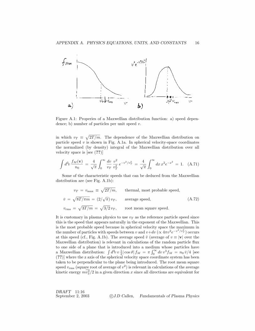
APPENDIX A. PHYSICS EQUATIONS, UNITS, AND CONSTANTS 16
Figure A.1: Properies of a Maxwellian distribution function: a) speed depen-dence; b) number of particles per unit speed v.
in which vT ≡ √2T/m. The dependence of the Maxwellian distribution onparticle speed v is shown in Fig. A.1a. In spherical velocity-space coordinatesthe normalized (by density) integral of the Maxwellian distribution over allvelocity space is [see (??)]∫
d3vfM (v)
n0=
4√π
∫ ∞
0
dv
vT
v2
v2T
e−v2/v2T =
4√π
∫ ∞
0dx x2e−x2
= 1. (A.71)
Some of the characteristic speeds that can be deduced from the Maxwelliandistribution are (see Fig. A.1b):
vT = vmax ≡ √2T/m, thermal, most probable speed,
v =√
8T/πm = (2/√π) vT , average speed,
vrms =√
3T/m =√
3/2 vT , root mean square speed.
(A.72)
It is customary in plasma physics to use vT as the reference particle speed sincethis is the speed that appears naturally in the exponent of the Maxwellian. Thisis the most probable speed because in spherical velocity space the maximum inthe number of particles with speeds between v and v+dv (∝ 4πv2e−v2/v2
T ) occursat this speed (cf., Fig. A.1b). The average speed v (average of v ≡ |v| over theMaxwellian distribution) is relevant in calculations of the random particle fluxto one side of a plane that is introduced into a medium whose particles havea Maxwellian distribution:
∫d3v v 1
2 | cosϑ| fM = π∫∞0 dv v3fM = n0 v/4 [see
(??)] where the z axis of the spherical velocity space coordinate system has beentaken to be perpendicular to the plane being introduced. The root mean squarespeed vrms (square root of average of v2) is relevant in calculations of the averagekinetic energy mv2
x/2 in a given direction x since all directions are equivalent for
DRAFT 11:16September 2, 2003 c©J.D Callen, Fundamentals of Plasma Physics

APPENDIX A. PHYSICS EQUATIONS, UNITS, AND CONSTANTS 17
an isotropic Maxwellian distribution (v2x = v2
y = v2z = v2
T /2 = v2/3 ≡ v2rms/3):
mv2x
2≡ 1
n0
∫d3v
(mv2
x
2
)fM (v) =
mv2rms
6=
T
2,
one-dimensional particle thermal energy. (A.73)
The total thermal energy of a particle is given by
mv2
2≡ 1
n0
∫d3v
(mv2
2
)fM (v) =
mv2rms
2=
3 T
2,
three-dimensional particle thermal energy. (A.74)
Finally, the kinetic pressure embodied in the Maxwellian distribution is
p ≡∫
d3v (mv2x)fM (v) =
∫d3v
(mv2
3
)fM (v) =
nv2rms
3= n T,
kinetic pressure. (A.75)
Entropy is the state of disorder of a closed system. It never decreaseswith time: it remains constant for reversible (e.g., Hamiltonian dynamics) pro-cesses, but increases for irreversible processes. Irreversible increases in theentropy of a system are caused by dissipative processes such as the cumula-tive effects of a large number of random collisions. For a system of weaklyinteracting, free particles the entropy is given by the logarithm of the aver-age volume [= 1/ρ0 — see (A.67)] of six-dimensional phase space occupied bya single particle, i.e., s = ln(1/ρ0). [For quantum mechanical systems it isthe logarithm of the number of statistically independent states, which is quan-tized to be the number of states that fit in the relevant phase space volume:Nqm =
∫d3Np d3Nq e−H(p,q)/T /(N !h3N ) in which h is Planck’s constant and
N is the number of degrees of freedom for the system being considered.] Thus,neglecting constants and using ρ0 = n0(m/2πT )3/2 ∼ n0/v3
T for an x,v phasespace, for classical systems one has
s = ln (1/ρ0) = ln (T 3/2/n0) + constant, entropy. (A.76)
For a volume V of uniform density (i.e., n0 = 1/V ) monotonic gas, the entropyis given by
s = lnV + (3/2) lnT + constant,
which, when multiplied by the molar gas constant R = kBNA is the conventionalform of the entropy for an ideal gas. Alternatively, writing T = p/n0 in (A.76)so that s = (3/2) ln(pV 5/3) + constant, one obtains the constant entropy (isen-tropic) equation of state pV Γ = constant for an ideal gas in a three-dimensionalsystem where Γ = 5/3.
Standard intermediate level textbooks for statistical mechanics are:
Kittel, Elementary Statistical Physics (1958) [?]
DRAFT 11:16September 2, 2003 c©J.D Callen, Fundamentals of Plasma Physics

APPENDIX A. PHYSICS EQUATIONS, UNITS, AND CONSTANTS 18
Reif, Fundamentals of Statistical and Thermal Physics (1965) [?]
Callen, Thermodynamics (1960) [?]
Kittel and Kroemer, Thermal Physics (1960). [?]
Some advanced level books on statistical mechanics are:Huang, Statistical Mechanics (1963) [?]
Tolman, The Principles of Statistical Mechanics (1938) [?]
Landau and Lifshitz, Statistical Physics (1959) [?]
Prigogine, Introduction to Thermodynamics of Irreversible Processes (1961). [?]
A.4 Kinetic Theory of Gases
Kinetic theory is a rigorous formalism that is used to provide a description ofthe behavior of a large collection of neutral molecules (or atoms) in a gas, partic-ularly when the assumptions of equilibrium statistical mechanics are not valid.In kinetic theory d3x d3v f(x,v, t) is the (assumed large) number of moleculeslocated in the six-dimensional (x,v) phase space with spatial positions lyingbetween x and x + dx and velocity vectors lying between v and v + dv, attime t. The quantity f(x,v, t), which has units of #/(m3·m3/s3), is called thedistribution function. It is governed by the equation
d f(x,v, t)dt
=∂f
∂ t+ v·∇f +
Fm
·∇vf =δf
δ t
)c
, kinetic equation (A.77)
in which F/m is the acceleration of a molecule due to the force F [e.g., theconservative force in (A.2)], ∇v ≡ ∂/∂v|x,t is the gradient in velocity space,and δf/δ t)c ∼ −νf represents the effects of “abrupt,” binary (microscopic)collisions at rate ν that result from force fields not included in F.
The (mathematical) characteristics of the first order differential operator (inthe 7 variables x,v, t) on the left of (A.77) represent the trajectories of themolecules in the absence of collision effects. The first order differential equa-tions governing the trajectories of the particles can be most generally writtenusing Hamilton’s equations. Thus, the kinetic equation for f(q,p, t), where p isthe canonical momentum defined in (A.13) and q is the canonically conjugateposition vector or for f(z, t) where z ≡ (q,p) = (x,p) is a six-dimensional vari-able that represents all of phase space, can be written most generally in termsof the Hamiltonian variables:
d f(q,p, t)dt
=∂f
∂ t+
dqdt
· ∂f∂q
+dpdt
· ∂f∂p
=∂f
∂ t+
dzdt
· ∂f∂z
=δf
δ t
)c
,
or, using Hamilton’s equations [see (A.15)], as
d f(q,p, t)dt
=∂f
∂ t+∂H
∂p· ∂f∂q
− ∂H∂q
· ∂f∂p
=δf
δ t
)c
, kinetic equation,
(A.78)
DRAFT 11:16September 2, 2003 c©J.D Callen, Fundamentals of Plasma Physics

APPENDIX A. PHYSICS EQUATIONS, UNITS, AND CONSTANTS 19
Particle motion in the z ≡ (p,q) six-dimensional Hamiltonian phase space isincompressible:
∂
∂z· dz
dt=∂
∂x· dx
dt+∂
∂p· dp
dt=∂
∂x· ∂H∂p
− ∂
∂p· ∂H∂x
= 0,
phase space incompressibility. (A.79)
Thus, the kinetic equation can also be written in the “conservative” form
d f(q,p, t)dt
=∂f
∂ t+∂
∂q·(
dqdt
f
)+∂
∂p·(
dpdt
f
)=∂f
∂ t+∂
∂z·(
dzdt
f
)=δf
δ t
)c
.
(A.80)
In the absence of collisions, or for time scales shorter than the collision time,the solution of (A.77) or (A.78) is that f must be a function of the constants ofthe motion — see (A.18), (A.19). For “collisionless” cases where the potentialsφ,A do not change in time and the Hamiltonian is the only constant of motion,the solution is f = f [H(p,q)] = f [H(z)]. Assuming further that there are alarge number of molecules which are interacting weakly (e.g., via collisions) withan even larger number of molecules that have a thermodynamic temperature T ,and hence that the requirements for the validity of statistical mechanics aresatisfied, the distributions given in (A.67) and (A.68) can be derived from thekinetic theory of gases.
The microscopic binary collision effects are most generally represented by
δf
δ t
)c
= CBf(x,v, t)
≡∫
d3v′∫
dΩdσ
dΩ| v − v′| [ f(v1)f(v′
1) − f(v)f(v′) ] ,
Boltzmann collision operator, (A.81)
in which v,v′ and v1,v′1 are the velocities of the colliding particles before and
after the collision and dσ/dΩ is the differential scattering cross-section for thecollisions [cf., (A.30)]. Here, for simplicity f(x,v, t) has been written as f(v)inside the collision operator. In deriving the Boltzmann collision operator it isassumed that the force F on the left of (A.77) is negligible during the collisionprocess, that the gas is sufficiently dilute so that binary or two-body collisionprocesses are predominant (i.e., three-body and many-body collisions or collec-tive particle interactions are negligible), and that the collisions only change thevelocity vectors of the particles (i.e., the collisions abruptly scatter the veloc-ity vectors of the particles at a given “point” x, t along a particle trajectory).The Boltzmann collision operator is a bilinear [because of f(v)f(v′)], integraloperator in velocity space. In the absence of radiative effects, since binary colli-sions conserve particle number, momentum mv and energy mv2/2, so does theBoltzmann collision operator:∫
d3vΨ(v) CB(f) = 0 for Ψ(v) = 1, mv, mv2/2. (A.82)
DRAFT 11:16September 2, 2003 c©J.D Callen, Fundamentals of Plasma Physics
APPENDIX A. PHYSICS EQUATIONS, UNITS, AND CONSTANTS 20
The functions Ψ(v) are sometimes called summational invariants because linearcombinations of them are also invariants of the collision operator.
For homogeneous (∇f = 0) gases in equilibrium (∂f/∂ t = 0) with noexternal forces on the molecules (F = 0), the kinetic equation (A.77) becomes
0 =δf
δ t
)c
= CB(f0), (A.83)
where the subscript zero on f indicates the equilibrium or lowest order solution.The general solution of this equation is
f0 = fM (v) = n0
(m
2πT0
)3/2
e−m|v−V0|2/2T0 =n0e−|v−V0|2/v2
T
π3/2v3T
,
Maxwellian distribution. (A.84)
This Maxwellian differs from the statistical mechanics result in (A.70) only byits explicit inclusion of the macroscopic flow velocity V0 of the gas (V0 ≡∫
d3v vf0/n0), which is not present in (A.70) because that result is obtainedin the rest frame of the gas (i.e., in the V0 rest frame). However, the result isarrived at by different methodologies in statistical mechanics and kinetic theory.Kinetic theory provides the more extendable framework for investigating morecomplicated situations that do not satisfy the assumptions used in deriving(A.70) and (A.84).
The Boltzmann collision operator also has the important property of irre-versibility: entropy increases until the distribution function is given by (A.84).Specifically, taking the entropy functional to be −f ln f and defining HB ≡∫
d3v f ln f , it can be shown that
dHB
dt=∫
d3v∂f
∂ t(1 + ln f) =
∫d3v CB(f) ln f ≤ 0,
Boltzmann H-theorem, (A.85)
with the equal sign being applicable only when f becomes equal to the equilib-rium, Maxwellian distribution given in (A.84).
In situations close to thermodynamic equilibrium the lowest order distribu-tion is the Maxwellian given by (A.84) and the distortions of the distributionfunction are higher order and small. In order to understand he nature of thesedistortions and to obtain approximate solutions of the kinetic equation (A.77)for this situation, consider the expansion of the distribution in a combination ofLaguerre and Legendre polynominials (see Appendix B), which are the completeorthogonal basis functions for speed (with the weighting function v2e−v2/v2
T thatcomes from the lowest order Maxwellian distribution in spherical velocity space)
DRAFT 11:16September 2, 2003 c©J.D Callen, Fundamentals of Plasma Physics
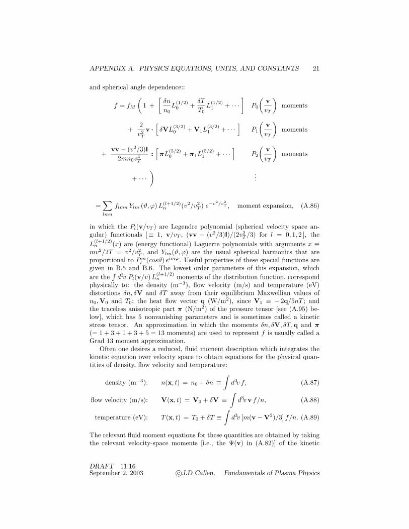
APPENDIX A. PHYSICS EQUATIONS, UNITS, AND CONSTANTS 21
and spherical angle dependence::
f = fM
(1 +
[δn
n0L(1/2)
0 +δT
T0L(1/2)
1 + · · ·]
P0
(vvT
)moments
+2v2
T
v ·[δVL(3/2)
0 + V1L(3/2)1 + · · ·
]P1
(vvT
)moments
+vv − (v2/3)I
2mn0v4T
:[πL(5/2)
0 + π1L(5/2)1 + · · ·
]P2
(vvT
)moments
+ · · ·) ...
=∑lmn
flmn Ylm (ϑ,ϕ) L(l+1/2)n (v2/v2
T ) e−v2/v2T , moment expansion, (A.86)
in which the Pl(v/vT ) are Legendre polynomial (spherical velocity space an-gular) functionals [≡ 1, v/vT , (vv − (v2/3)I)/(2v2
T /3) for l = 0, 1, 2 ], theL(l+1/2)
n (x) are (energy functional) Laguerre polynomials with arguments x ≡mv2/2T = v2/v2
T , and Ylm(ϑ,ϕ) are the usual spherical harmonics that areproportional to Pm
l (cosϑ) eimϕ. Useful properties of these special functions aregiven in B.5 and B.6. The lowest order parameters of this expansion, whichare the
∫d3v Pl(v/v)L(l+1/2)
n moments of the distribution function, correspondphysically to: the density (m−3), flow velocity (m/s) and temperature (eV)distortions δn, δV and δT away from their equilibrium Maxwellian values ofn0,V0 and T0; the heat flow vector q (W/m2), since V1 ≡ − 2q/5nT ; andthe traceless anisotropic part π (N/m2) of the pressure tensor [see (A.95) be-low], which has 5 nonvanishing parameters and is sometimes called a kineticstress tensor. An approximation in which the moments δn, δV, δT,q and π(= 1 + 3 + 1 + 3 + 5 = 13 moments) are used to represent f is usually called aGrad 13 moment approximation.
Often one desires a reduced, fluid moment description which integrates thekinetic equation over velocity space to obtain equations for the physical quan-tities of density, flow velocity and temperature:
density (m−3): n(x, t) = n0 + δn ≡∫
d3v f, (A.87)
flow velocity (m/s): V(x, t) = V0 + δV ≡∫
d3v v f/n, (A.88)
temperature (eV): T (x, t) = T0 + δT ≡∫
d3v [m(v − V2)/3] f/n. (A.89)
The relevant fluid moment equations for these quantities are obtained by takingthe relevant velocity-space moments [i.e., the Ψ(v) in (A.82)] of the kinetic
DRAFT 11:16September 2, 2003 c©J.D Callen, Fundamentals of Plasma Physics
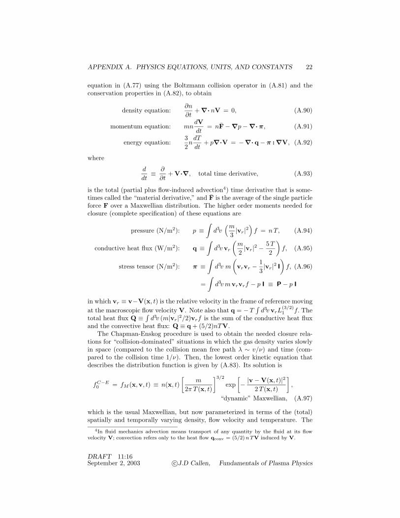
APPENDIX A. PHYSICS EQUATIONS, UNITS, AND CONSTANTS 22
equation in (A.77) using the Boltzmann collision operator in (A.81) and theconservation properties in (A.82), to obtain
density equation:∂n
∂t+ ∇· nV = 0, (A.90)
momentum equation: mndVdt
= nF − ∇p − ∇· π, (A.91)
energy equation:32n
dT
dt+ p∇·V = −∇· q − π : ∇V, (A.92)
where
d
dt≡ ∂
∂t+ V·∇, total time derivative, (A.93)
is the total (partial plus flow-induced advection4) time derivative that is some-times called the “material derivative,” and F is the average of the single particleforce F over a Maxwellian distribution. The higher order moments needed forclosure (complete specification) of these equations are
pressure (N/m2): p ≡∫
d3v(m
3|vr|2
)f = n T, (A.94)
conductive heat flux (W/m2): q ≡∫
d3v vr
(m
2|vr|2 − 5 T
2
)f, (A.95)
stress tensor (N/m2): π ≡∫
d3v m
(vrvr − 1
3|vr|2 I
)f, (A.96)
=∫
d3v mvrvrf − p I ≡ P − p I
in which vr ≡ v−V(x, t) is the relative velocity in the frame of reference movingat the macroscopic flow velocity V. Note also that q = −T
∫d3v vrL
(3/2)1 f. The
total heat flux Q ≡ ∫ d3v (m|vr|2/2)vrf is the sum of the conductive heat fluxand the convective heat flux: Q ≡ q + (5/2)nTV.
The Chapman-Enskog procedure is used to obtain the needed closure rela-tions for “collision-dominated” situations in which the gas density varies slowlyin space (compared to the collision mean free path λ ∼ v/ν) and time (com-pared to the collision time 1/ν). Then, the lowest order kinetic equation thatdescribes the distribution function is given by (A.83). Its solution is
fC−E0 = fM (x,v, t) ≡ n(x, t)
[m
2π T (x, t)
]3/2
exp[− |v − V(x, t)|2
2 T (x, t)
],
“dynamic” Maxwellian, (A.97)
which is the usual Maxwellian, but now parameterized in terms of the (total)spatially and temporally varying density, flow velocity and temperature. The
4In fluid mechanics advection means transport of any quantity by the fluid at its flowvelocity V; convection refers only to the heat flow qconv = (5/2) n TV induced by V.
DRAFT 11:16September 2, 2003 c©J.D Callen, Fundamentals of Plasma Physics

APPENDIX A. PHYSICS EQUATIONS, UNITS, AND CONSTANTS 23
conductive heat flux q and anisotropic stress π vanish for fC−E0 . Thus, in order
to determine these needed closure relations, it is necessary to determine the firstorder distortion of the distribution function: δf ≡ f − fC−E
0 . (Note that, byconstruction, since the total density n flow velocity V and temperature T arebuilt into fC−E
0 , the density, momentum and energy moments of δf vanish:∫d3v δf = 0,
∫d3v mv δf = 0,
∫d3v (mv2/2) δf = 0, C-E consraints.
(A.98)
The kinetic equation for δf is obtained by substituting the definition f =fC−E0 + δf into (A.77), making use of the density, momentum and energy con-
servation equations to remove the dependences on ∂n/∂ t, ∂V/∂ t and ∂T/∂ t.Neglecting higher order corrections that are inversely proportional to the colli-sion frequency, the result is
CB(δf) '[(
m|vr|22T
− 52
)vr ·(
1T
∇T
)+
m
TW :(vrvr − |vr|2
3I
)]fC−E0 ,
(A.99)
in which, as above, vr ≡ v − V(x, t), and
W ≡ 12[∇V + (∇V)T
]− 13
I (∇·V) , rate of strain tensor, (A.100)
which is caused by gradients in the flow velocity V and has units of per sec-ond. The normalized temperature gradient ∇ lnT and rate-of-strain tensor Ware called thermodynamic forces — because they induce distortions δf of thedistribution function away from a dynamic Maxwellian and hence away fromthermodynamic equilibrium. Note that beacause of the invariants of the Boltz-mann collision operator given in (A.82), a proper solution of (A.99) for δf willsatisfy the Chapman-Enskog constraints in (A.98).
The Boltzmann collision operator needs to be specified in detail in orderto properly solve (A.99). However, the nature of the solution for δf can beexhibited by using an approximate collision model:
CK(δf) = − ν δf ≡ − ν (f − fC−E0 ), Krook-type collision operator
(A.101)
in which
ν ≡ nσv, collision frequency, (A.102)
where the overbar indicates the “reaction rate” σv has been averaged over aMaxwellian distribution. Using this collision operator in (A.99), solving forδf and using the definitions in (A.95) and (A.96) yields the needed closure(constituitive) relations for the fluid moment equations (A.90)–(A.92):
q = −κm∇T, κm ≡ nχm, χm =54
v2T
ν=
54νλ2, conductive heat flux,
(A.103)
DRAFT 11:16September 2, 2003 c©J.D Callen, Fundamentals of Plasma Physics

APPENDIX A. PHYSICS EQUATIONS, UNITS, AND CONSTANTS 24
which is in the form of a Fourier law for the heat flux and
π = − 2 µmW, µm =12
nmv2
T
ν=
12
nm νλ2, viscous stress, (A.104)
in which
λ ≡ vT /ν, collision mean free path, (A.105)
has been defined for thermal molecules. In these closure relations, κm is theheat conduction coefficient, χm is the heat diffusivity and µm is the viscositycoefficient. The superscript m on the various coefficients indicate that theyarise from the micoscopic (molecular) processes of discrete collisions in the gas.Equations (A.103) and (A.104) give the thermodynamic fluxes q,π inducedby the thermodynamic forces ∇T,W. If the appropriate Boltzmann collisionoperator is used instead of the approximate Krook-type model of (A.101), thescaling of the κm, χm, and µm “molecular diffusion” coefficients with collisionfrequency and thermal speed remains the same; however the numerical factorsin (A.103) and (A.104) change slightly.
The reference cross section σ for atomic and molecular collisions is σ0 ≡πa2
0 ∼ 10−20 m2 in which a0 is the Bohr (atomic) radius (A.154). For standardtemperature and pressure (STP) air at the earth’s surface, the average crosssection for molecular collisions is σ ∼ 40σ0 ∼ 4× 10⁻¹⁹ m2, the density is nn ∼2.5× 1025 m−3, and the thermal speed is vT ∼ 300 m/s. Thus, for standard airν ∼ nσvT ∼ 3×10⁹ s−1, λ ∼ vT /ν ∼ 10−7 m, and µm/nm ∼ νλ2/2 ∼ 1.5×10⁻⁵
m2/s, χm ∼ (5/2)(µm/nm).The Chapman-Enskog analysis is valid as long as the collision mean free
path is short compared to the gradient scale lengths (i.e., λ |∇ lnT | << 1,λ |∇V|/|V| << 1) and temporal variations are slow compared to the collisiontime [e.g., ν−1(∂ lnn/∂t) << 1]. Substituting the closure relations given in(A.103) and (A.104) into the momentum and energy conservation equationsyields (neglecting for simplicity the small effects due to gradients of the transportcoefficients κm and µm):
mndVdt
= nF − ∇(
p − µm
3∇·V
)+ µm∇2V, (A.106)
32
dT
dt+ T (∇·V) = χm∇2T + 2
µm
n|W|2 . (A.107)
The diffusive components of these equations indicate that the “molecular” diffu-sion coefficients for momentum (viscous) and heat diffusion are µm/nm and χm,both of which scale as νλ2 and have units of m2/s. A physical interpretation ofthe processes and parametric scalings that underly these diffusion coefficientsare given in the next section.
An equation can also be developed for the evolution of the collisional entropys which is dimensionless and is defined in kinetic theory for f ' fC−E
0 by
s ≡ − 1n
∫d3v f ln f = ln
(T 3/2
n
)+ constant, collisional entropy. (A.108)
DRAFT 11:16September 2, 2003 c©J.D Callen, Fundamentals of Plasma Physics

APPENDIX A. PHYSICS EQUATIONS, UNITS, AND CONSTANTS 25
Note that this entropy is the negative of the Boltzmann HB function [see (A.85)]and yields the same result as that obtained from equilibrium statistical mechan-ics [see (A.76)]. Taking the total time derivative of this equation yields, uponsubstituting in (A.90) and (A.92),
nTds
dt=
32n
dT
dt− T
dn
dt= T
[∂(ns)∂t
+ ∇· (nsV)]
= −∇· q − π :∇V, entropy evolution. (A.109)
Alternatively, since the flow of entropy density (entropy flux) is nsV + q/T ,after using the density conservation relation (A.90) and the rate-of-strain tensordefinition (A.100),
∂(ns)/∂t + ∇· (nsV + q/T ) = θ ≡ − (1/T ) [q ·∇ lnT + π : W ] (A.110)
in which θ represents the rate of entropy production due to dissipative (irre-versible) processes, which is positive definite and caused by the thermodynamicfluxes q,π flowing in response to the thermodynamic forces ∇ lnT , W.
For the closure relations given in (A.103) and (A.104) the entropy produc-tion rate simplifies to (again neglecting gradients in the transport coefficientsκm, µm):
θ = nχm |∇ lnT |2 + 2 µm |W|2 , entropy production rate. (A.111)
Thus, entropy is produced by the microcopic collisional processes that diffusivelyrelax the gradients of the temperature and flow velocity in the gas. The entropyproduction rate is small under the Chapman-Enskog approximations (large ν,small λ = vT /ν): ds/dt ∼ νλ2 |∇ lnT |2 << ν if heat conduction effects aredominant, or ds/dt ∼ νλ2 |∇V|2 /v2
T << ν if viscous flow damping is domi-nant. Hence, for processes that are rapid compared to the collisional entropyproduction rate and where the entropy flow induced by the conductive heatflux q is negligible (e.g., in a constant temperature gas), it is sufficient to usethe “adiabatic” or isentropic (i.e., non-dissipative, constant entropy) equationof state for an ideal gas obtained from setting ds/dt = 0:
d
dtln(
T 3/2
n
)=
d
dtln(
p3/2
n5/2
)= 0 =⇒ p
nΓ= constant,
isentropic (“adiabatic”) equation of state, (A.112)
where Γ is 5/3 for the three-dimensional system being considered, but in generalis given by Γ = (N + 2)/N in which N is the number of degrees of freedom inthe system. [In thermodynamics Γ ≡ cP /cV is the ratio of the heat capacity(≡ ∂u/∂T ) at constant pressure to that at constant volume.] Note that for aconstant density gas of volume V = 1/n, (A.112) becomes the familiar equationof state for an ideal gas: pV Γ = constant. The adiabatic or isentropic equationof state can be used in place of the energy balance equation (A.92) or (A.107)for studies of rapid, isentropic processes because there is no significant entropyproduction or heat flow for such processes.
DRAFT 11:16September 2, 2003 c©J.D Callen, Fundamentals of Plasma Physics
APPENDIX A. PHYSICS EQUATIONS, UNITS, AND CONSTANTS 26
Most of the previously noted standard textbooks on statistical mechanicsprovide intermediate level descriptions of the kinetic theory of gases. Advancedlevel textbooks and monographs that deal specifically with the kinetic theoryof gases include:
Chapman and Cowling, The Mathematical Theory of Non-Uniform Gases (1952)[?]
H. Grad, “Principles of the Kinetic Theory of Gases,” in Handbuch der Physik ,Volume 12 (Springer-Verlag, Berlin, 1957) [?]
R. Herdan and B. S. Liley, “Dynamical Equations and Transport Relationshipsfor a Thermal Plasma,” Rev. Mod. Phys. 32, 731 (1960). [?]
A.5 Stochastic Processes, Diffusion
The heat and momentum diffusion produced by the collision-induced randomsteps or motions of molecules in a gas can be understood in terms of a stochasticor random walk process. Such processes are often called Brownian motion (aftera botanist Robert Brown who, in 1827, observed irregular motions of smallcolloidal size particles immersed in a fluid), or more formally a Markoff process(no memory of previous history or steps).
For a simple one-dimensional mathematical model of the random walk pro-cess, assume that between collisions (or another random process) a moleculemoves a distance ∆x in a random direction (to the right or left) in a time ∆t.For such a process the position xn of a molecule after the nth step is related tothe position xn−1 after the previous step by
xn = xn−1 + Rn ∆x (A.113)
in which Rn is randomly ±1. Using this mapping equation as a recursion rela-tion, one finds that after N random steps the difference of the final position xN
from the initial position x0 becomes
xN = x0 + ∆xN∑
n=1
Rn. (A.114)
In the limit of a large number N of random steps one obtains:
limN→∞
∣∣∣∣xN − x0
N∆x
∣∣∣∣ = limN→∞
|∑n Rn|N
= limN→∞
O(1)N
= 0, (A.115)
because Rn is randomly ±1. Thus, after a large number N of random stepsthe average position of a molecule does not deviate much (<< N∆x) from itsinitial position x0.
However, as illustrated in Fig. A.2, the random steps do have an effect:they cause such molecules to wander randomly in the x direction, to ever largerdistances from x0 as the number N of random steps increases. Thus, after a largenumber of random steps the position of a molecule is described by a probability
DRAFT 11:16September 2, 2003 c©J.D Callen, Fundamentals of Plasma Physics
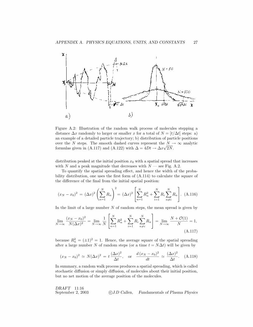
APPENDIX A. PHYSICS EQUATIONS, UNITS, AND CONSTANTS 27
Figure A.2: Illustration of the random walk process of molecules stepping adistance ∆x randomly to larger or smaller x for a total of N = [t/∆t] steps: a)an example of a detailed particle trajectory; b) distribution of particle positionsover the N steps. The smooth dashed curves represent the N → ∞ analyticformulas given in (A.117) and (A.122) with ∆ = 4Dt → ∆x
√2N .
distribution peaked at the initial position x0 with a spatial spread that increaseswith N and a peak magnitude that decreases with N — see Fig. A.2.
To quantify the spatial spreading effect, and hence the width of the proba-bility distribution, one uses the first form of (A.114) to calculate the square ofthe difference of the final from the initial spatial position:
(xN − x0)2 = (∆x)2(
N∑n=1
Rn
)2
= (∆x)2 N∑
n=1
R2n +
N∑i=1
Ri
N∑n '=i
Rn
. (A.116)
In the limit of a large number N of random steps, the mean spread is given by
limN→∞
(xN − x0)2
N(∆x)2= lim
N→∞1N
N∑n=1
R2n +
N∑i=1
Ri
N∑n '=i
Rn
= limN→∞
N + O(1)N
= 1,
(A.117)
because R2n = (±1)2 = 1. Hence, the average square of the spatial spreading
after a large number N of random steps (or a time t = N∆t) will be given by
(xN − x0)2 ' N(∆x)2 = t(∆x)2
∆t, or
d (xN − x0)2
dt' (∆x)2
∆t. (A.118)
In summary, a random walk process produces a spatial spreading, which is calledstochastic diffusion or simply diffusion, of molecules about their initial position,but no net motion of the average position of the molecules.
DRAFT 11:16September 2, 2003 c©J.D Callen, Fundamentals of Plasma Physics
APPENDIX A. PHYSICS EQUATIONS, UNITS, AND CONSTANTS 28
However, in an inhomogeneous medium there is, on average, a net motionor flux of particles. The particle transport flux produced by a large numberof molecules undergoing such random walk processes in a neutral gas with aspatially varying density n = n(x) can obtained as follows. In a time ∆t theplane x = x0 will be traversed by the half (on average) of the molecules thatexperience collisions in the layer between x0−∆x and x0, and which are movingto the right (+). Thus, the flux (Γ ≡ nV = n dx/dt) of molecules moving to theright is
Γ+ =12
∫ x0
x0−∆xn(x)
dx
∆t=
∆x
2∆t
[n(x0) − ∆x
2dn
dx
∣∣∣∣x0
+ · · ·]
in which the density n(x) has been expanded in a Taylor series about x0. Sim-ilarly, the flux of molecules moving through the x = x0 plane to the left (−)is
Γ− =12
∫ x0+∆x
x0
n(x)dx
∆t=
∆x
2∆t
[n(x0) +
∆x
2dn
dx
∣∣∣∣x0
+ · · ·]
.
The net particle flux is the difference between these two fluxes:
Γ = Γ+ − Γ− = −Ddn
dx
∣∣∣∣x0
, Fick’s diffusion law. (A.119)
For the simple model being considered D is given by
D =(∆x)2
2∆t, diffusion coefficient, (A.120)
which has units of m2/s. Thus, the diffusion coefficient D is half the rate ofspatial spreading for a random walk process — see (A.118).
The natural step size ∆x for the motion of molecules between collisions ina neutral gas is λ, the collision mean free path. The characteristic time ∆tbetween collisions of molecules is 1/ν. Thus, one infers from (A.120) that thescaling of diffusivities induced by molecular collisions should be D ∼ νλ2, whichwas what was obtained in (A.103) and (A.104) in the preceding section. In amonoatomic neutral gas there are heat and momentum diffusivities but there isno particle diffusivity (or particle flux Γ) because, while two colliding moleculesexchange energy and momentum during the molecular collisions, the density ofmolecules is usually unchanged as a result of the collisions.
In more realistic situations different molecules may have different ∆x and∆t values; then one must take an appropriate average and D = 〈(∆x)2〉/(2∆t).Since the parametric scaling of the diffusion coefficient is quite general, but ap-propriate averages are often difficult to formulate or evaluate for various physicalprocesses, the expression for D in (A.120) is mostly used to infer the scalingof the diffusion coefficient with physical parameters. Then, kinetic calculationsare used to obtain the relevant numerical coefficients — the “headache factors.”
DRAFT 11:16September 2, 2003 c©J.D Callen, Fundamentals of Plasma Physics

APPENDIX A. PHYSICS EQUATIONS, UNITS, AND CONSTANTS 29
In the presence of this random walk process induced by molecular collisions,the equation for the density n(x, t) [see (A.90] becomes ∂n/∂t+∂(nVx)/∂x = 0.Using the Fick’s diffusion law (A.116) for nVx = Γ yields a one-dimensionaldiffusion equation:
∂n
∂t=∂
∂xD∂n
∂x, diffusion equation. (A.121)
To illustrate the properties of solutions of this equation, imagine that a smallnumber δN of molecules are added to the medium at the position x0: n(x, 0) =δNδ(x−x0). After a short time, the appropriate (Green-function-type) solutionof (A.121) is
n(x, t) = δNe−(x−x0)
2/4Dt
√π√
4Dt, short-time diffusive distribution, (A.122)
as can be verified by direct substitution. Note that this distribution of particleshas the desired properties for a random walk process and represents it well inthe N → ∞ limit — see Fig. A.2b. In particular, it is peaked at x = x0 andspreads spatially and decreases in magnitude as time progresses. In a time t(assumed >> ∆t) the average spreading of the molecules in the x direction is
(x − x0)2 ≡∫∞−∞ dx (x − x0)2 n(x, t)∫∞
−∞ dx n(x, t)= 4Dt
∫∞0 dy y2e−y2∫∞0 dy e−y2 = 2Dt =
(∆x)2
∆tt
(A.123)
in which y ≡ (x − x0)/√
4Dt and the integrals have been evaluated using (??).Note that this rate of spatial spreading of the density agrees with that inferredabove for the random walk process of a molecule — (A.118).
The Gaussian character of this distribution can be emphasized by writingthe short time diffusive density response in (A.122) in the form
n(x, t) = δNe−(x−x0)
2/∆2
√π∆
, ∆ ≡ √4Dt. (A.124)
In this form one readily sees from (??) that in the t → 0 limit the solutionbecomes a delta function (see Section B.2) at x = x0: limt→0 n(x, t)=δN δ(x −x0), which was the initial condition. Also, in terms of ∆ the root mean squarespatial spread becomes simply
δxrms ≡(
(x − x0)2)1/2
=√
2Dt =∆√2
= ∆x
√t
∆t= ∆x
√N,
root mean square spatial spread. (A.125)
The last result shows that, as indicated in Fig. A.2, the spatial spreading isproportional to the square root of the number of random walk steps.
DRAFT 11:16September 2, 2003 c©J.D Callen, Fundamentals of Plasma Physics

APPENDIX A. PHYSICS EQUATIONS, UNITS, AND CONSTANTS 30
Using these formulas, note also that the average time t required for moleculesto diffuse a distance δx ≡ x − x0 from the initial position x0 is
t ∼ (δx)2
2 D∼(δx
∆x
)2
∆t, time to diffuse a distance δx. (A.126)
Hence, the time t required to diffuse a short distance δx is the product of the ba-sic random walk time ∆t times (δx/∆x)2 — the square of the number of randomwalk steps ∆x in the distance δx to be traversed. This quadratic dependenceof the spreading time on the spreading distance is an intrinsic property of dif-fusive processes. As a caveat on this analysis, note that the solution (A.122)is only valid for short times: t < L2
n/D ∼ (Ln/∆x)2∆t — so the backgroundmedium density and diffusion coefficient are reasonably constant over the dis-tance ∆/
√2 =
√2Dt = ∆x
√t/∆t that typical particles spread over in the time
t [i.e., (∆/n)(dn/dx) ≡ ∆/Ln << 1 and (∆/D)(dD/dx) << 1].In a finite box, as time progresses molecules eventually diffuse to the bound-
aries of the box where it will be assumed the molecules are absorbed. Thequestion then becomes: what is the average confinement time for molecules inthe box? Assume for simplicity that: the diffusion coefficient is constant inspace; a one-dimensional treatment is sufficient; δN molecules are inserted atthe center (x = 0) of a box of width 2L (assumed >> ∆x = λ) at time t = 0;and the density of molecules vanishes at the box boundaries (x = ±L). Then,the solution of the diffusion equation (A.121) for this boundary value problemcan be shown (by separation of variables, expansion in sinusoidal eigenfunctions)to be
n(x, t) =δN
L
∞∑j=0
e−t/τj cos(λj
x
L
), with λj ≡ (2j + 1)π
2, τj ≡ L2
λ2jD
. (A.127)
For short times (t << τ0) the box boundaries at x = ±L are unimportantand this solution reduces to (A.124), which is a more convenient form then.For intermediate times (t ∼ τj) the sinusoidal eigenfunctions (up to at least2j) must be summed to obtain the response. In the time asymptotic limit(t > τ0 > τ1 > τ2 · · · ) the lowest order eigenmode solution dominates:
n(x, t)t>τ0' δN
Le−t/τ0 cos
(π2
x
L
). (A.128)
Thus, an average ”confinement time” for molecules in the box can be identifiedas
τ0 ≡ L2
λ20D
=L2
(π/2)2D' L2
2.5D, confinement time. (A.129)
Note that upon using D = (∆x)2/2∆t one obtains τ0 = (2/λ20)(L/∆x)2∆t,
which quantifies (for this specific case where δx → L, t → τ0) the “headachefactors” in the scaling relation (A.126). For cylindrical, spherical “boxes” the
DRAFT 11:16September 2, 2003 c©J.D Callen, Fundamentals of Plasma Physics

APPENDIX A. PHYSICS EQUATIONS, UNITS, AND CONSTANTS 31
eigenfunctions are Bessel, spherical Bessel functions and the lowest order eigen-values are λ0 ' 2.405,λ0 = π, respectively. Then, using a as the radius of the“box,” one obtains confinement times of τ0 ' a2/6D, a2/10D for cylindrical,spherical systems, respectively.
Many of the references noted at the end of the two preceding sections havediscussions of random walk (Brownian motion) and stochastic diffusion pro-cesses. The classic and ageless reference for such processes is:
S. Chandrasekhar, “Stochastic Problems in Physics and Astronomy,” Rev. Mod.Phys. 15, 1 (1943). [?]
A.6 Fluid Mechanics
The equations of “hydrodynamics” used to describe the behavior of a fluid arethe fluid moment equations obtained from the kinetic theory of gases — (A.90),(A.91) and (A.112). However, they are usually modified by writing them interms of the mass density ρm ≡ n m, which has units of kg/m3:
mass continuity equation:∂ρm
∂t+ ∇· ρmV = 0, (A.130)
Navier-Stokes equation: ρmdVdt
= ρmFm
− ∇p′ + µm∇2V, (A.131)
(momentum balance)
isentropic equation of state:d
dtln(
p
ρΓm
)= 0, (A.132)
in which p′ ≡ p − (µm/3)∇·V. (The equation of state is often called the“adiabatic” equation of state in hydrodynamics.) In these equations d/dt is thetotal time derivative taking account both of the direct temporal derivative andthe effects of the advection by the flow velocity V in the fluid:
d
dt≡ ∂
∂t+ V·∇, total time derivative. (A.133)
For gases or liquids in the earth’s atmosphere the relevant force on moleculesis the gravitational force, which is a conservative force:
FG = FG = −m∇VG ' −mg ex ≡ mg, gravitational force, (A.134)
where VG = −MEG/R is the gravitational potential. In the last expression usehas been made of the fact that near the earth’s surface (x ≡ R − RE << RE ,radius of the earth) one has VG ' −(MEG/R2
E)(RE − x + · · · ). Also, here,g ≡ (MEG/R2
E) ' 9.81 m/s2 is the gravitational acceleration at the earth’ssurface.
The velocity flow field V can in general be decomposed into parts repre-sentable in terms of scalar, vector potentials ψ, C (see Section D.5):
V = −∇ψ + ∇×C, potential representation of a flow field. (A.135)
DRAFT 11:16September 2, 2003 c©J.D Callen, Fundamentals of Plasma Physics

APPENDIX A. PHYSICS EQUATIONS, UNITS, AND CONSTANTS 32
The scalar potential part represents the longitudinal, irrotational or compress-ible part of the flow since ∇·V = −∇·∇ψ = −∇2ψ. The vector potentialpart is incompressible since ∇·∇×C = 0. However, this component represents“rotation” or vorticity5 (units of s−1) in the flow:
ω ≡ ∇×V = ∇×(∇×C), vorticity. (A.136)
The properties of sound waves in a fluid can be illustrated by consideringcompressible perturbations of air in the earth’s atmosphere. The equilibriumpressure distribution is determined from the “hydrostatic” force balance equi-librium, which is the equilibrium (∂/∂t = 0) and small viscosity limit of theNavier-Stokes equation that in the absence of equilibrium flows (V0 = 0) be-comes simply:
0 = − ρm0∇VG − ∇p0.
Assuming for simplicity that the temperature T is constant, taking x to bethe vertical distance above the earth’s surface, and using p = nT = ρm0T/m(Boyle’s law for this situation), the hydrostatic equilibrium becomes
0 = − ρm0g − T
m
dρm0
dx=⇒ ρm0(x) = ρm0(0) e−mgx/T ,
law of atmospheres. (A.137)
Thus, in equilibrium the density of air decreases with distance above the surfaceof the earth on a scale length of T/mg = v2
T /2g ∼ 104 m.To exhibit the properties of sound waves consider perturbations of the com-
pressible air in this equilibrium:
ρm = ρm0 + ρm, V = V, p = p0 + p, perturbed equilibrium, (A.138)
in which the tilde over a quantity indicates the perturbation in that quantity.Substituting these forms into the fluid equations (A.130)–(A.132) yields, uponneglecting the effect of gravity for simplicity and linearizing the equations (i.e.,neglecting all quantities that are quadratic or higher order in the perturbations):
∂ρm
∂t+ ρm0∇·V + V·∇ρm0 = 0, ρm0
∂V∂t
= −∇p + µm∇2V, p = cHS
2ρm
where
cHS ≡
√Γp0/ρm0 =
√ΓT/m, hydrodynamic sound speed, (A.139)
which is typically about 340 m/s at the earth’s surface. Note that for a neutralgas cH
S =√Γ/2 vT . For an equilibrium that is approximately homogeneous
over the collision mean free path λ (λ |∇ ln ρm0| << 1), a perturbed density5A physical example of vorticity is the circular flow of water around a drain in a bathtub
as it is being emptied.
DRAFT 11:16September 2, 2003 c©J.D Callen, Fundamentals of Plasma Physics

APPENDIX A. PHYSICS EQUATIONS, UNITS, AND CONSTANTS 33
response ρm exists only for compressible perturbations (∇·V 0= 0). For suchperturbations these equations can be combined to yield
∂2ρm
∂t2− ∇·
(cHS
2∇ρm − µm∇2V)
= 0.
Considering perturbations that are localized relative to the scale length of theequilibrium density gradient so that the ∇cH
S2 and ∇µm terms can be neglected,
but longer scale than the collision mean free path (typically ∼ 10−7 m for air atthe earth’s surface) so the viscosity can be neglected (i.e., cH
S2/g ∼ 104 m >>
perturbation scale length >> λ ∼ 10−7 m), this equation becomes simply
∂2ρm
∂t2− cH
S2∇2ρm = 0, sound wave equation. (A.140)
Thus, density perturbations compress (∇·V < 0) and rarefy (∇·V > 0) thefluid as they propagate through it adiabatically (with negligible entropy pro-duction) at the sound speed cH
S defined in (A.139).To exhibit the properties of the most fundamental type of fluid instabilities,
the Rayleigh-Taylor (R-T) instabilities, consider perturbations of nearly incom-pressible liquids, in a case where a heavy liquid is above a lighter liquid andthe two fluids are immiscible. For incompressible (∇·V → 0) perturbations thelinearized continuity equation becomes
∂ρm
∂t= − V·∇ρm0, advective response, (A.141)
which indicates the change in local mass density caused by a perturbed flowin the direction of the gradient in the equilibrium mass density. Combiningthis advective response with the partial time derivative of the linearized Navier-Stokes equation yields
ρm0∂2V∂t2
=(V·∇ρm0
)∇VG − ∇∂p
∂t.
Taking the curl of this equation to eliminate the perturbed pressure gradient andhence the coupling to sound waves, and neglecting gradients in the equilibriumcompared to those in the perturbations (ρm0∇×V >> ∇ρm0×V) and viscosityeffects (valid for perturbation scale lengths long compared to the collision meanfree path λ), yields for the perturbed flow vorticity ω ≡ ∇×V:
ρm0∂2ω
∂t2= ∇
(V·∇ρm0
)×∇VG.
Considering a coordinate system where x is directed vertically upward and y, zare in a plane parallel to the earth’s surface, and assuming wavelike pertur-bations of the type V = ∇×C = − ez×∇Cz, in which C = Czez, Cz ∼exp(ik·x − iωt) with kx << ky is a stream function [see (??,??)], so thatω = − ez∇2
⊥Cz ' ezk2yCz, yields an equation for the perturbation frequency:
ω2 ' −∇VG ·∇ ln ρm0 = g ·∇ρm. (A.142)
DRAFT 11:16September 2, 2003 c©J.D Callen, Fundamentals of Plasma Physics
APPENDIX A. PHYSICS EQUATIONS, UNITS, AND CONSTANTS 34
When ∇VG ·∇ρm0 < 0 (light liquid above heavy liquid since ∇VG ≡ −g isupward), ω2 is positive and two benign, oscillating waves occur. (Adding vis-cosity effects causes the waves to be damped.) However, when a heavy liquid isplaced over a light liquid (∇VG ·∇ρm0 = −g ·∇ρm0 > 0) the ω2 < 0 indicatescomplex conjugate roots, one of which will be growing exponentially in time atrate:
γ ≡ Imω ' (−g ·∇ ln ρm0)1/2, R-T instability growth rate (A.143)
This is the Rayleigh-Taylor (or interchange) instability by which the interfaceregion between the upper heavy fluid and the lower lighter fluid develops growingundulations that lead ultimately to interchange of the positions of the heavy andlight fluids.
The overall process of the interchange of the two fluids can be thought ofas consisting of the following steps. First, thermal fluctuations excite a modestundulation of the boundary between the two liquids. If the heavy fluid is on top,this spontaneous perturbation grows exponentially in time at the rate indicatedby (A.143). The undulations grow to a large amplitude where the linearizationprocedure used to derive (A.142) becomes invalid. Lagrangian coordinates (i.e.,coordinates that follow particular fluid elements as they move rather than theusual fixed position Eulerian ones) can be used to explore the growth of thestructures into the slightly nonlinear regime. However, ultimately the vortex-like collective motions of the fluids become highly nonlinear, very contorted andlarge enough to encounter adjacent vortices and/or the boundaries of the regionsoccupied by the fluids. Then, turbulence in the fluid develops and it cascadesthe large vortices into smaller ones, turbulently mixing the two fluids until theheavier one is on the bottom.
In order to describe the behavior of the vortices as they evolve nonlinearlytoward the turbulent state, consider the total time derivative of the circulationCK ≡ ∮C d" ·V in the rotational part of the flow V, which is responsible for thevortex, over the closed curve C within the fluid:
dCK
dt≡ d
dt
∮C
d" ·V =d
dt
∫∫S
dS · ∇×V
=∫∫
SdS · [(∂/∂t + V·∇) (∇×V)] +
∫∫S(dS/dt) ·∇×V
=∫∫
SdS · ∇×(∂V/∂t) − ∇× [V× (∇×V)]
=∫∫
SdS · [∂ω/∂t − ∇×(V×ω)] (A.144)
in which use has been made of Stokes’ theorem (??), S is the open surfacebounded by the closed curve C that moves with the encompassed fluid, dS/dt =(∇·V)dS − ∇V· dS [see (??)], and the vector identity in (??) has been used.Dividing the Navier-Stokes equation (A.131) with a conservative force F by ρm
DRAFT 11:16September 2, 2003 c©J.D Callen, Fundamentals of Plasma Physics
APPENDIX A. PHYSICS EQUATIONS, UNITS, AND CONSTANTS 35
and taking its curl to obtain an equation for ∇×∂V/∂t yields, after makinguse of (??):
dCK
dt=∫∫
SdS ·(
1ρ2m
∇ρm×∇[p − µm
3(∇·V)
]+ ∇×µm
ρm∇2V
). (A.145)
For an adiabatic equation of state (A.132), p ∝ ρmΓ and hence ∇ρm×∇p = 0.
Thus, the circulation CK is constant in time, except for the dissipative effectsdue to viscosity that are small for all but very short scale lengths of the order ofthe collision mean free path λ because µm/ρm ∼ νλ2. Thus, on most relevantscale lengths
dCK
dt= 0 for µm → 0, Kelvin’s circulation theorem, (A.146)
for inviscid (zero viscosity) fluids.What this theorem shows is that a vortex tube moves with (or is “frozen
into”) the fluid as it evolves, and that the amount of circulation CK in the flowfield V remains constant — except for the effects of viscosity, which becomesimportant in boundary layers near the edge of the fluid or at the edge of vorticesthat come close to other vortices. However, the derivation relied on the use ofStokes’s theorem, which required that the topology of the closed curve C becontinuous and that it remain so. Thus, the invariance of CK could be brokenby nonlinear interactions between vortex structures that break or reconnect thetopology by causing the bounding curve C, which is expected to always movewith the fluid and encompass the same vorticity flux
∫∫S dS ·∇×V, to become
discontinuous. To the extent that the topology of the surfaces of vorticity fluxremains intact there is no motion (or transport) of fluid relative to these surfaces.However, the flux surfaces of the vorticity can distort in shape as they movearound in the fluid. Thus, vortex tubes or eddies are relatively robust objectsin low viscosity fluids.
The nonlinear evolution and interactions of vortices in a fluid are governedby the vorticity evolution equation
∂ω
∂t= ∇×(V×ω) − ω (∇·V) +
µm
ρm∇2ω (A.147)
or,dω
dt≡(∂
∂t+ V·∇
)ω = ω ·∇V +
µm
ρm∇2ω. (A.148)
These equations are obtained by taking the curl of (A.131), which eliminates thecoupling to sound waves, and assuming for simplicity that the mass density isconstant. The ∇×(V×ω) term in (A.147) represents the advection of the vor-ticity vector ω by the flow velocity V — as indicated by the last line of (A.144).The ω ·∇V term on the right of (A.148) represents vortex tube stretching bygradients in the velocity flow; it vanishes for two-dimensional flows. In three-dimensional flows the vortex tube stretching term reduces the area of a vortex
DRAFT 11:16September 2, 2003 c©J.D Callen, Fundamentals of Plasma Physics

APPENDIX A. PHYSICS EQUATIONS, UNITS, AND CONSTANTS 36
but also increases its vorticity — to keep the vorticity flux CK constant asrequired by Kelvin’s circulation theorem.
The ratio of the nonlinear advection of vorticity [∇×(V×ω), a nonlinear“inertia” term] to the viscous dissipation of vorticity (µm∇2ω) is
Re =∇×(V×ω)
(µm/ρm)∇2ω∼ ρm0V0L0
µm, Reynolds number, (A.149)
in which V0, L0 are typical flow speeds and gradient scale lengths in the fluid.When the vorticity evolution equation is written in terms of dimensionless vari-ables, the reciprocal of the Reynolds number is the only dimensionless parameterin the equation — as the coefficient of the viscous dissipation term. For example,for incompressible flows (i.e., ones that do not excite sound waves and are dom-inated by vorticies), Eq. (A.147) can be written in terms of the dimensionlessvariables t ≡ (V0/L0)t, V ≡ V/V0, and ∇ ≡ L0∇ as
∂ω
∂ t= ∇×(V×ω) +
1Re
∇2ω. (A.150)
Thus, all incompressible flows with the same Reynolds number and the same flowgeometry will have the same flow properties. At low Reynolds numbers (Re <∼ 1)the flow is laminar. For not too large Reynolds numbers vortex structuresinduced by the particular geometrical situation (e.g., flow past a fixed body)tend to dominate the flow pattern. For high Reynolds numbers (Re >∼ 103) thenonlinear vorticity advection overwhelms the viscous dissipation and the flowbecomes turbulent.
In fully developed turbulence (Re >> 103) there is a cascade of energyfrom macroscopically-induced large-scale vortices through nonlinear interactionsof turbulent eddies of successively smaller dimensions until the scale lengthsbecome so small that the energy in the eddies is viscously dissipated. (Theeffective Reynolds number is close to unity for the dissipative scale eddies.)Since the dominant eddy interaction term is the vortex stretching term ω ·∇V in(A.148), successive “generations” of the turbulent eddies become longer, thinnerand have larger vorticities. Thus, the mean square vorticity, which is known asthe enstrophy (Ω ≡ |ω|2), increases during the cascade.
For sufficiently large Reynolds numbers there is a large “inertial” range ofspatial scale lengths for which the vortex interactions are predominantly non-linear (i.e., where the large-scale “stirring” and small-scale viscous dissipationeffects are negligible). In the inertial range the turbulent eddies are self-similar(i.e., of the same structure, independent of scale size, from one generation to thenext one). The energy flow per unit mass ε = (V·∇)(V 2/2) from one wavenum-ber range k to the next smaller one can be estimated by εk ∼ kV 3
k ∼ V 2k /τk
in which τk ∼ (kVk)−1 is the turbulent decorrelation or eddy turnover timeat a given k. Since energy is input via “stirring” at large scales and dissi-pated at small scales, in steady-state the energy transfer rate from one scaleto the next smaller one in the inertial range must be nearly constant. Thus,εk ' ε ∼ V 3
0 /L0, a constant for a given externally driven situation, and hence
DRAFT 11:16September 2, 2003 c©J.D Callen, Fundamentals of Plasma Physics

APPENDIX A. PHYSICS EQUATIONS, UNITS, AND CONSTANTS 37
Vk ∼ (ε/k)1/3. The energy E(k) in the turbulent fluctuations between k and2k is given approximately by
∫dk E(k) ∼ k E(k) ∼ V 2
k or E(k) ∼ ε2/3k−5/3,which is the Kolomogorov spectrum for turbulence within a large inertial range.The successively smaller scale eddies have smaller velocities and energies, butlarger vorticity and faster turnover rates [τk ∼ (kVk)−1 ∼ (εk2)−1/3] to keepthe energy flow rate in k-space constant.
In the inertial range the turbulent eddies lose their momentum on a mixinglength scale ∆k ∼ Vkτk ∼ 1/k. This leads to a Prandtl mixing length esti-mate for the effective diffusion coefficient [cf., (A.120)] for turbulent viscosityin the fluid of Deff ∼ µeff/ρm ∼ ∆2
k/τk ∼ ε1/4/k4/3. However, this turbu-lent mixing is actually dissipationless; all it does is transfer the momentumand energy to shorter scale lengths. Eventually, the eddies reach the (Kolo-mogorov) dissipation scale k−1
d at which 1/τkd ∼ (µm/ρm) k2d, which yields
kd ∼ ε1/4/(µm/ρm)3/4 ∼ (Re)3/4/L0.Because the effects of viscosity are negligible in the inertial range and because
the viscous dissipation scale length is so short [k−1d ∼ L0/(Re)3/4 << L0], it
is tempting to neglect it entirely. However, while its effects can be neglectedfor inertial range scale lengths (1/L0 << k << kd), it must be retained ingeneral because it: 1) increases the order of the differential equation governingvorticity; 2) is important in boundary layers near material objects and othernearby vortices; and, 3) most importantly for computer simulation, providesthe only energy sink (at high k) for turbulent fluctuations in a neutral fluid.
Most of the previously noted standard textbooks on mechanics, statisticalmechanics and kinetic theory of gases contain introductory or intermediate leveldescriptions of fluid mechanics. Advanced level monographs and textbooks thatspecifically deal with fluid mechanics include:
Batchelor, Introduction to Fluid Dynamics (1967) [?]
Tennekus and Lumley, A First Course in Turbulence (1972) [?].
A.7 Quantum Mechanical Effects
The fundamental concept in quantum mechanics is that, owing to the wavelikenature of particles on small scale lengths, a particle’s position q and canonicallyconjugate momentum p cannot simultaneously be known to arbitrarily high ac-curacy. Rather, the product of the uncertainties in the position and momentum,δq and δp, respectively, must be Planck’s constant or greater:
δp · δq ≥ h, Heisenberg uncertainty principle. (A.151)
This relation shows the limit of applicability of mechanical causality. The un-certainty principle holds for any pair of canonically conjugate variables. Thus,it applies for energy and time, which for conservative systems are canonicallyconjugate variables (p = H = ε and q = t), as well:
δε δt ≥ h. (A.152)
DRAFT 11:16September 2, 2003 c©J.D Callen, Fundamentals of Plasma Physics
APPENDIX A. PHYSICS EQUATIONS, UNITS, AND CONSTANTS 38
By Heisenberg’s uncertainty principle, the position of a nonrelativistic particlemoving with velocity v in a force-free region (so that its canonical momentump is simply mv) cannot be known to within
λh = h/mv, de Broglie wavelength. (A.153)
In the Bohr model of the hydrogen atom an electron gyrates at constantradius a0 around the proton nucleus of the atom. Since the rotational angle ϕ isa symmetry coordinate and hence totally uncertain, the Heisenberg uncertaintyprinciple requires that the canonically conjugate action J be quantized to integermultiples (n) of Planck’s constant:
J =∮
p · dq =∮
pϕ dϕ = 2πme a20 ω0 = n h
in which the angular momentum pϕ ≡ me a20 ω0 where ω0 ≡ dϕ/dt is the con-
stant rotation frequency. The equilibrium radial force balance between theelectric field force e2/(4πε0a2
0) and the centripital acceleration force me a0 ω20
on the electron yields the equation
e2
4πε0a20
= me a0 ω20 .
Solving these two simultaneous equations for a0 in the ground state (n = 1)case yields the characteristic radius of the hydrogen atom:
a0 = 4πε0 (h/2π)2
me e2' 0.529×10⁻¹⁰ m, Bohr radius. (A.154)
This is the characteristic scale length for the “size” of all atoms — the rangeover which their electrostatic force field extends. The corresponding range overwhich nuclear forces extend is
re =e2
4πε0mec2' 2.82×10⁻¹⁵ m, classical electron radius, (A.155)
which is inferred from equating the electric potential energy ∼ e2/(4πε0re)from a distributed electron charge to the electron rest mass energy mec2.
The binding energy of an electron in a Bohr atom in its ground (lowestenergy) state is given by the (negative of the) potential energy of the electronwhen it is located at the Bohr radius from the proton plus the kinetic energy ofthe electron:
EH∞ =
e2
4πε0a0− me
2a20ω
20 =
14πε02
mee4
2(h/2π)2' 13.6 eV,
Bohr atom binding energy, (A.156)
which is also called the Rydberg energy. For electrons in the nth quantumstate the orbit radius increases by a factor of n2 and the rotation frequency
DRAFT 11:16September 2, 2003 c©J.D Callen, Fundamentals of Plasma Physics
APPENDIX A. PHYSICS EQUATIONS, UNITS, AND CONSTANTS 39
ω0 decreases by a factor of 1/n3; consequently, the binding energy of the statedecreases by a factor of 1/n2. For electrons gyrating around an ion of charge Zi,the potential and consequently the electric field force increases by a factor of Zi.This causes the Bohr radius to decrease by a factor of 1/Zi and the ionizationenergy to increase by a factor of Z2
i . Thus, neglecting fine-structure effects, thebinding energy of an outer electron in a level labeled by the quantum numbern (≥ 1) which is gyrating around an ion of charge Zi is given by
EZ∞(n) ' Z2
i EH∞/n2, outer electron binding energy. (A.157)
Note that for a nucleus with a high atomic number Z the binding energy ofthe most tightly bound (n = 1, ground state) electron, which is the last oneto be removed as an atom is ionized, can be very large. For example, for iron(Z = 26) the binding energy of the last electron is ∼ 9 keV while for tungsten(Z = 74) it is ∼ 75 keV.
The degree of ionization in a plasma can be estimated from the Saha equationwhich gives the population density of a particular ionization and quantum stateof an atom in a gas in thermodynamic equilibrium. It can be obtained by equat-ing the rates of ionization [∝ nn exp(−Ui/Te)] and recombination [∝ ni(neλ3
h)]for ions in a partially ionized gas:
ni
nn' 2
ne
(2πmeTe
h2
)3/2
e−Ui/Te = 25/2 neλ3De
(nea30)1/2
e−Ui/Te
' 6 × 1027
ne(m−3)[Te(eV)]3/2 e−Ui/Te , Saha equation, (A.158)
in which ne, ni and nn are the electron, ion and neutral density, respectively,Ui is the ionization potential and Te is the temperature in electron volts of theassumed Maxwellian distribution of electrons. The ionization potential Ui forionization of an atom from its ground (neutral) state to the first ionized stateis given by the electron binding energy in the atom [cf., Eq. (A.157)]. It rangesfrom 3.9 eV for Cesium atoms to 24.6 eV for Helium.
The fractional ionization [≡ ni/(nn +ni)] is exponentially small for electrontemperatures Te much lower than the ionization potential Ui. The electrontemperature required to attain a small degree of ionization (∼ ni/nn << 1) canbe estimated by solving the Saha equation iteratively for Te:
Te|ion ' Ui
ln(
6 × 1027 [Te(eV)]3/2
(ni/nn)ne(m−3)
) ∼ (0.02–1) Ui, (A.159)
where in the last form the smallest number correponds to interplanetary densi-ties (∼ 106 m−3) and the largest to solid densities (∼ 1029 m−3). The Te requiredto produce a fully ionized state (ni/nn >> 1) is not much larger. Thus, for ex-ample, a nitrogen gas (Ui = 14.5 eV) at a density of 2.5×1025 m−3 (the densityof room temperature air) becomes 1% ionized at Te ' 1.4 eV, and fully ionizedfor Te
>∼ 2.2 eV. At lower densities the electron temperature range over which
DRAFT 11:16September 2, 2003 c©J.D Callen, Fundamentals of Plasma Physics
APPENDIX A. PHYSICS EQUATIONS, UNITS, AND CONSTANTS 40
the transition from a partially to fully ionized gas takes place is even narrower.For some examples of the variation with electron density of the Te required forcomplete ionization, see Fig. ?? at the end of Chapter 1.
Note however that the ions might not be fully stripped of their electrons. Inparticular, for Te ∼ 0.1–10 keV, high Z ions might not be fully stripped becauseof the very large binding energy of their most tightly bound electrons. Suchions would have an ion charge Zi < Z.
Some standard introductory level quantum mechanics textbooks are:
Krane, Modern Physics ( ) [?]
Sproul and Phillips, Modern Physics ( ) [?]
Tipler, Modern Physics ( ) [?]
Gasiorowicz, Quantum Physics ( ) [?]
Powell and Crasemann, Quantum Mechanics ( ) [?].
DRAFT 11:16September 2, 2003 c©J.D Callen, Fundamentals of Plasma Physics

APPENDIX A. PHYSICS EQUATIONS, UNITS, AND CONSTANTS 41
A.8 Physical Constants
Fundamental Physical ConstantsRelativeUncertainty
Quantity Symbol Best Value6 (×10−6)
electron mass me 9.109 389 7 × 10⁻³¹ kg 0.59proton mass mp 1.672 623 1 × 10⁻²⁷ kg 0.59elementary charge e 1.602 177 33 × 10−19 C 0.30speed of light in vacuum c 299 792 458 m/s exact7permeability of vacuum µ0 4π × 10−7 H/m exactpermittivity of vacuum ε0 1/µ0c2 F/m exactgravitational constant G 6.672 59 × 10−11 N ·m2/kg2 128Planck constant h 6.626 075 5 × 10⁻³⁴ J · s 0.60Boltzmann constant kB 1.380 658 ×10−23 J/K 8.5
SI Units And Their Abbreviations, Interrelationships
Quantity Name Symbol In Terms Of Other Units
length meter m 102 cm = 1010 Amass kilogram kg 103 gtime second selectric current ampere A C/stemperature kelvin K ' 1/11 604.4 eVamount of substance mole molatomic unit of energy electron volt eV ' 1.602 177 33 × 10−19 Jatomic unit of mass amu u ' 1.660 540 2 × 10⁻²⁷ kgfrequency hertz Hz s−1 (cycles per second)force newton N m · kg · s−2
pressure, stress pascal Pa N/m2 = m−1· kg · s−2
energy, work joule J N ·m = m2· kg · s−2
power watt W J/s = m2· kg · s−3
electric charge coulomb C s ·Aelectric potential volt V W/A = m2· kg · s−3·A−1
capacitance farad F C/V = m−2· kg−1· s4·A2
electrical resistance ohm Ω V/A = m2· kg · s−3·A−2
magnetic flux weber Wb V · s = m2· kg · s−2·A−1
magnetic flux density8 tesla T Wb/m2 = kg · s−2·A−1
inductance henry H Wb/A = m2· kg · s−2·A−2
6E.R. Cohen and B.N. Taylor, Physics Today, August 1998, BG7 [?].7The speed of light fixes the length of the meter in terms of the second.8In plasma physics magnetic field strengths are often quoted in Gauss: 1 Tesla ≡ 10 kGauss.
DRAFT 11:16September 2, 2003 c©J.D Callen, Fundamentals of Plasma Physics
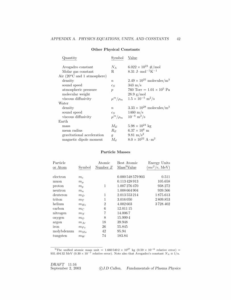
APPENDIX A. PHYSICS EQUATIONS, UNITS, AND CONSTANTS 42
Other Physical Constants
Quantity Symbol Value
Avogadro constant NA 6.022 × 10²³ #/molMolar gas constant R 8.31 J ·mol−1K−1
Air (20oC and 1 atmosphere)density n 2.49 × 1025 molecules/m3
sound speed cS 343 m/satmospheric pressure p 760 Torr = 1.01 × 10⁵ Pamolecular weight 28.9 g/molviscous diffusivity µm/ρm 1.5 × 10⁻⁵ m2/s
Waterdensity n 3.33 × 1028 molecules/m3
sound speed cS 1460 m/sviscous diffusivity µm/ρm 10−6 m2/s
Earthmass ME 5.98 × 1024 kgmean radius RE 6.37 × 10⁶ mgravitational acceleration g 9.81 m/s2magnetic dipole moment Md 8.0 × 10²² A ·m2
Particle Masses
Particle Atomic Best Atomic Energy Unitsor Atom Symbol Number Z Mass9Value (mc2/e, MeV)
electron me 0.000 548 579 903 0.511muon mµ 0.113 428 913 105.658proton mp 1 1.007 276 470 938.272neutron mn 1.008 664 904 939.566deuteron mD 1 2.013 553 214 1 875.613triton mT 1 3.016 050 2 809.853helium mHe 2 4.002 603 3 728.402carbon mC 6 12.011 15nitrogen mN 7 14.006 7oxygen mO 8 15.999 4argon mAr 18 39.948iron mFe 26 55.845molybdenum mMo 42 95.94tungsten mW 74 183.84
9The unified atomic mass unit = 1.660 540 2 × 1027 kg (0.59 × 10⁻⁶ relative error) =931.494 32 MeV (0.30 × 10⁻⁷ relative error). Note also that Avogadro’s constant NA ≡ 1/u.
DRAFT 11:16September 2, 2003 c©J.D Callen, Fundamentals of Plasma Physics

APPENDIX B. SPECIAL FUNCTIONS 1
Appendix B
Special Functions
Key properties of special functions as they are often used in plasma physics aresummarized in this appendix.
B.1 Heaviside Step Function
The Heaviside step function is usually just called the step function. It was intro-duced by Oliver Heaviside in the late 1800s to represent the idealized switchingon (in time) of a voltage or other source in electrical engineering problems. Itis defined by
H(x − x0) =
1, x > x0,0, x < x0.
(B.1)
At x = x0, H is in general undefined (because it is discontinuous there), butwill be taken to be 1/2 there so that it is equal to its average value at this jumpdiscontinuity. The derivative of the Heaviside step function is the Dirac deltafunction:
H ′(x − x0) = δ(x − x0) (B.2)
in which the prime denotes differentiation with respect to the argument. The xdependence of the step and delta functions are shown schematically in Fig. B.1.
B.2 Dirac Delta Function
The Dirac delta function, which is usually just called the delta function, is aconcentrated “spike” or impulse of unit area. It was introduced by P.A.M. Diracin the 1920s in the context of developing a physical interpretation of quantummechanics. The delta function is often used in plasma physics to represent thespatial distribution of “point” charged particles. It also arises naturally fromintegrals that yield singular responses to resonant perturbations.
DRAFT 22:15February 2, 2002 c©J.D Callen, Fundamentals of Plasma Physics

APPENDIX B. SPECIAL FUNCTIONS 2
Figure B.1: Schematic of x dependence of the Heaviside step function and Diracdelta function.
The one-dimensional delta function is defined by the following properties:
δ(x − x0) = 0 for x #= x0,∫ b
adx f(x) δ(x − x0) =
f(x0), a < x0 < b,0, otherwise, (B.3)
for any function f(x) that is continuous at x = x0. Thus, the delta functionis zero except at the point where its argument vanishes; there it is so large(i.e., singular) that the integral of it over that point (its area) is unity [i.e., forf(x) = 1 we have
∫ ba dx δ(x − x0) = 1]. Note that hence the delta function has
units of one over the units of its argument.The delta function is a mathematically improper function — because it is
unbounded where its argument vanishes. However, it is a generalized functionwhose integral can be defined through a limiting process in distribution theory.Specifically, for a unity area distribution function w(x), one defines a deltasequence w(x;∆) which becomes progressively more peaked (height ∼ 1/∆)and narrower (width ∼ ∆) in the limit that ∆→ 0 such that it becomes a unitarea “spike.” In terms of such a delta sequence, one defines∫ b
adx δ(x) f(x) ≡ lim
∆→0
∫ b
adx w(x;∆) f(x) = f(0). (B.4)
Symbolically, we can write
δ(x) .= lim∆→0
w(x;∆), (B.5)
which is only valid in evaluating integrals in the form given in (B.4).A function w(x) is a suitable basis for a delta sequence if it is nonnegative
and has unity area [∫ ∞−∞ dx w(x) = 1]. Oscillatory, unity area functions that
decay as their argument increases [lim|x|→∞ |w(x)| → 0] are also suitable basisfunctions for delta sequences. For a suitable distribution function w(x), a deltasequence is defined by w(x;∆) ≡ w(x/∆)/∆. Examples of delta sequences basedon Gaussian [wG = e−x2
/√
π ], Lorentzian [wL = 1/π(x2 + 1)] and correlation
DRAFT 22:15February 2, 2002 c©J.D Callen, Fundamentals of Plasma Physics
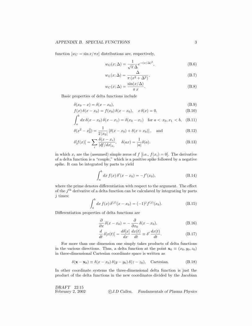
APPENDIX B. SPECIAL FUNCTIONS 3
function [wC = sinx/πx] distributions are, respectively,
wG(x;∆) =1√π∆
e−(x/∆)2 , (B.6)
wL(x;∆) =∆
π (x2 +∆2), (B.7)
wC(x;∆) =sin(x/∆)
π x. (B.8)
Basic properties of delta functions include
δ(x0 − x) = δ(x − x0), (B.9)f(x) δ(x − x0) = f(x0) δ(x − x0), x δ(x) = 0, (B.10)∫ b
adx δ(x − x0) δ(x − x1) = δ(x0 − x1) for a < x0, x1 < b, (B.11)
δ(x2 − x20) =
12 |x0| [δ(x − x0) + δ(x + x0)] , and (B.12)
δ[f(x)] =∑
i
δ(x − xi)|df/dx|xi
, δ(ax) =1|a|δ(a). (B.13)
in which xi are the (assumed) simple zeros of f [i.e., f(xi) = 0]. The derivativeof a delta function is a “couple,” which is a positive spike followed by a negativespike. It can be integrated by parts to yield∫ b
adx f(x) δ′(x − x0) = −f ′(x0), (B.14)
where the prime denotes differentiation with respect to the argument. The effectof the jth derivative of a delta function can be calculated by integrating by partsj times: ∫ b
adx f(x) δ(j)(x − x0) = (−1)jf (j)(x0). (B.15)
Differentiation properties of delta functions are
∂
∂xδ(x − x0) = − ∂
∂x0δ(x − x0), (B.16)
d
dtδ[x(t)] =
dδ[x]dx
dx(t)dt
≡ δ′dx(t)
dt. (B.17)
For more than one dimension one simply takes products of delta functionsin the various directions. Thus, a delta function at the point x0 ≡ (x0, y0, z0)in three-dimensional Cartesian coordinate space is written as
δ(x − x0) ≡ δ(x − x0) δ(y − y0) δ(z − z0), Cartesian. (B.18)
In other coordinate systems the three-dimensional delta function is just theproduct of the delta functions in the new coordinates divided by the Jacobian
DRAFT 22:15February 2, 2002 c©J.D Callen, Fundamentals of Plasma Physics
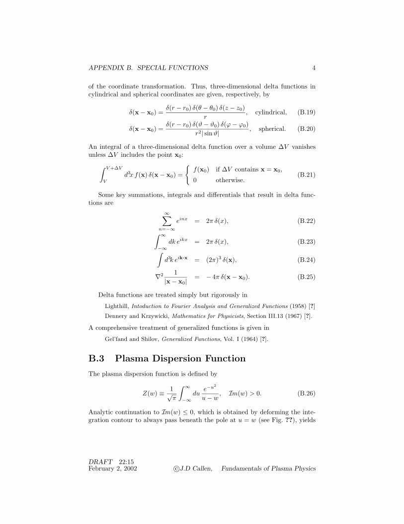
APPENDIX B. SPECIAL FUNCTIONS 4
of the coordinate transformation. Thus, three-dimensional delta functions incylindrical and spherical coordinates are given, respectively, by
δ(x − x0) =δ(r − r0) δ(θ − θ0) δ(z − z0)
r, cylindrical, (B.19)
δ(x − x0) =δ(r − r0) δ(ϑ − ϑ0) δ(ϕ − ϕ0)
r2| sinϑ| , spherical. (B.20)
An integral of a three-dimensional delta function over a volume ∆V vanishesunless ∆V includes the point x0:∫ V +∆V
Vd3x f(x) δ(x − x0) =
f(x0) if ∆V contains x = x0,
0 otherwise.(B.21)
Some key summations, integrals and differentials that result in delta func-tions are
∞∑n=−∞
einx = 2π δ(x), (B.22)∫ ∞
−∞dk eikx = 2π δ(x), (B.23)∫
d3k eik·x = (2π)3 δ(x), (B.24)
∇2 1|x − x0| = − 4π δ(x − x0). (B.25)
Delta functions are treated simply but rigorously in
Lighthill, Intoduction to Fourier Analysis and Generalized Functions (1958) [?]
Dennery and Krzywicki, Mathematics for Physicists, Section III.13 (1967) [?].
A comprehensive treatment of generalized functions is given in
Gel’fand and Shilov, Generalized Functions, Vol. I (1964) [?].
B.3 Plasma Dispersion Function
The plasma dispersion function is defined by
Z(w) ≡ 1√π
∫ ∞
−∞du
e−u2
u − w, Im(w) > 0. (B.26)
Analytic continuation to Im(w) ≤ 0, which is obtained by deforming the inte-gration contour to always pass beneath the pole at u = w (see Fig. ??), yields
DRAFT 22:15February 2, 2002 c©J.D Callen, Fundamentals of Plasma Physics
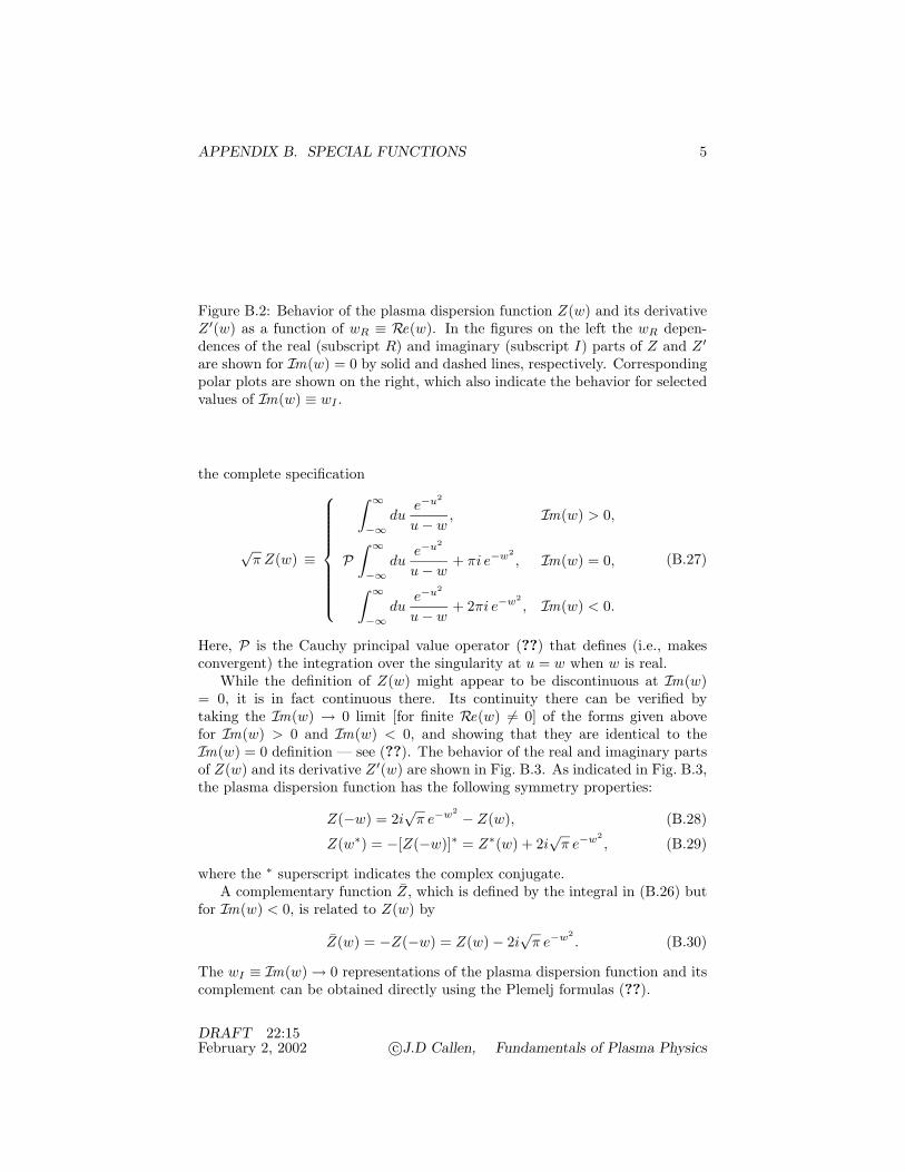
APPENDIX B. SPECIAL FUNCTIONS 5
Figure B.2: Behavior of the plasma dispersion function Z(w) and its derivativeZ ′(w) as a function of wR ≡ Re(w). In the figures on the left the wR depen-dences of the real (subscript R) and imaginary (subscript I) parts of Z and Z ′are shown for Im(w) = 0 by solid and dashed lines, respectively. Correspondingpolar plots are shown on the right, which also indicate the behavior for selectedvalues of Im(w) ≡ wI .
the complete specification
√π Z(w) ≡
∫ ∞
−∞du
e−u2
u − w, Im(w) > 0,
P∫ ∞
−∞du
e−u2
u − w+ πi e−w2
, Im(w) = 0,∫ ∞
−∞du
e−u2
u − w+ 2πi e−w2
, Im(w) < 0.
(B.27)
Here, P is the Cauchy principal value operator (??) that defines (i.e., makesconvergent) the integration over the singularity at u = w when w is real.
While the definition of Z(w) might appear to be discontinuous at Im(w)= 0, it is in fact continuous there. Its continuity there can be verified bytaking the Im(w) → 0 limit [for finite Re(w) #= 0] of the forms given abovefor Im(w) > 0 and Im(w) < 0, and showing that they are identical to theIm(w) = 0 definition — see (??). The behavior of the real and imaginary partsof Z(w) and its derivative Z ′(w) are shown in Fig. B.3. As indicated in Fig. B.3,the plasma dispersion function has the following symmetry properties:
Z(−w) = 2i√
π e−w2 − Z(w), (B.28)
Z(w∗) = −[Z(−w)]∗ = Z∗(w) + 2i√
π e−w2, (B.29)
where the ∗ superscript indicates the complex conjugate.A complementary function Z, which is defined by the integral in (B.26) but
for Im(w) < 0, is related to Z(w) by
Z(w) = −Z(−w) = Z(w) − 2i√
π e−w2. (B.30)
The wI ≡ Im(w) → 0 representations of the plasma dispersion function and itscomplement can be obtained directly using the Plemelj formulas (??).
DRAFT 22:15February 2, 2002 c©J.D Callen, Fundamentals of Plasma Physics

APPENDIX B. SPECIAL FUNCTIONS 6
An alternative definition of Z(w) that is valid for all finite Im(w) is
W (w) =Z(w)i√
π=
2 e−w2
√π
∫ ∞
−iwdt e−t2 = e−w2
[1 − erf(−iw)] ≡ e−w2erfc(−iw),
(B.31)which indicates the close relationship to the error function. This is the formof the plasma dispersion function most commonly used in the Russian plasmaphysics literature, and in error function reference books.
The plasma dispersion function satisfies the differential equation
Z ′(w) ≡ dZ
dw= − 2 [ 1 + w Z(w) ]. (B.32)
This differential equation can be used to write higher order derivatives in termsof lower order derivatives:
Z(n) ≡ dnZ
dwn= − 2
dn−1(wZ)dwn−1
= − 2[(n − 1)Z(n−2) + wZ(n−1)] for n ≥ 2.
(B.33)The plasma dispersion function has a power series expansion about w = 0
given by
Z(w) = i√
π e−w2 − w√
π∞∑
n=0
(−w2)n
Γ(n + 1/2)
= i√
π e−w2 − 2w
(1 − 2w2
3+
4w4
15− 8w6
105+ · · ·
). (B.34)
Its asymptotic expansion for |w| >> 1 is
Z(w) ∼ iσ√
π e−w2 − 1√π
∞∑n=0
w−(2n+1) Γ(n − 1/2)
= iσ√
π e−w2 − 1w
(1 +
12w2
+3
4w4+
158w6
+ · · ·)
(B.35)
where
σ ≡ 0, Im(w) > 0,
1, Im(w) = 0,2, Im(w) < 0.
(B.36)
Corresponding power series and asymptotic expansions for the derivative of theplasma dispersion function are given, respectively, by
Z ′ = −2iw√
π e−w2 − 2(1 − 2w2 + · · ·) for |w| << 1 and (B.37)
Z ′ ∼ −2iσw√
π e−w2+
1w2
(1 +
32w2
+ · · ·)
for |w| >> 1. (B.38)
Related, but more complicated integrals of the form
Zn(w) ≡ 1√π
∫ ∞
−∞du
un e−u2
u − w, n ≥ 0, (B.39)
DRAFT 22:15February 2, 2002 c©J.D Callen, Fundamentals of Plasma Physics

APPENDIX B. SPECIAL FUNCTIONS 7
can be calculated in terms of derivatives of Z(w) as follows. First, taking nsuccessive derivatives of Z(w) and integrating by parts n times one obtains
Z(n)(w) ≡ dnZ(w)dwn
=n!√π
∫ ∞
−∞du
e−u2
(u − w)n+1=
1√π
∫ ∞
−∞
du
u − w
dn(e−u2)
dun.
From the Rodrigues formula for Hermite polynomials Hn(u),
dn
dun(e−u2
) = (−1)n e−u2Hn(u),
it is clear that the nth derivative of Z(w) can be written as
dnZ(w)dwn
=(−1)n
√π
∫ ∞
−∞du
Hn(u) e−u2
u − w. (B.40)
Now, any power of the variable u can be expressed in terms of a series of Hermitepolynomials with orders up to and including the power of u through the relation
un =12n
M∑m=0
dm(n) Hn−2m(u), (B.41)
in which dm(n) are the coefficients given in Table 22.12 of Abromowitz andStegun [?] and the upper limit of the sum is M ≡ [n/2], the largest integer lessthan or equal to n/2. Substituting (B.41) into (B.39) and utilizing (B.40) yields
Zn(w) =12n
[n/2]∑m=0
(−1)n−2mdm(n)dn−2mZ(w)
dwn−2m.
The first four of these functions are
Z0(w) = Z (B.42)Z1(w) = −(1/2)Z ′ = 1 + wZ, (B.43)Z2(w) = (1/4)[2Z + Z ′′] = −(w/2)Z ′ = w + w2Z, (B.44)Z3(w) = −(1/8)[6Z ′ + Z ′′′] = (1/2)[1 + 2w2(1 + wZ)], (B.45)
in which the primes denote differentiation with respect to the argument and inthe last equalities we have made use of the definitions of differentials of Z givenin (B.32) and (B.33).
The plasma dispersion function is tabulated inFried and Conte, The Plasma Dispersion Function (1961) [?].
B.4 Bessel Functions
Bessel functions arise naturally from second order differential equations in theradial coordinate for a cylindrical geometry. Their governing differential equa-tion is
z2 d2y
dz2+ z
dy
dz+ (z2 − n2) y = 0 (B.46)
DRAFT 22:15February 2, 2002 c©J.D Callen, Fundamentals of Plasma Physics

APPENDIX B. SPECIAL FUNCTIONS 8
Figure B.3: Variation of the basic and modified Bessel functions with theirarguments.
in which z is the independent (radial coordinate) variable and n is an integer.The basic (fundamental) solution of this differential equation is y = Jn(z), whichis the Bessel function of the first kind of order n. The linearly independentsolution Yn(z) of (B.46) is called the Bessel function of the second kind oforder n. It is singular at z = 0. Hence it is not a valid solution for mostcylindrical geometry problems where the response must be finite at the origin ofthe cylindrical geometry (z ≡ r = 0). The z dependence of Jn for n = 0, 1, 2 isshown in Fig. B.4. The first few zeros [Jn(jn,i) ≡ 0] of the fundamental Besselfunctions are (for i = 1, 2, 3, · · ·)
j0,i = 2.405, 5.520, 8.654, · · · , j1,i = 3.832, 7.016, 10.173, · · · . (B.47)
Changing z from a real to an imaginary argument (z → iz) in (B.46) changesthe sign of the z2 term in the defining differential equation. The correspondingsolutions of this modified differential equation are the modified Bessel functionsof the first and second kind of order n, respectively: In(z) and Kn(z). Thevariation of e−zIn(z) with the argument z is shown for n = 0, 1, 2 in Fig. B.4.
Useful recursion relations for the basic Bessel functions include
Jn−1(z) + Jn+1(z) =2 n
zJn(z), (B.48)
Jn−1(z) − Jn+1(z) = 2J ′n ≡ 2
dJn(z)dz
, (B.49)
J−n(z) = (−1)nJn(z). (B.50)
Analogous recursion relations for the modified Bessel functions are:
In−1(z) − In+1(z) =2 n
zIn(z), (B.51)
In−1(z) + In+1(z) = 2 I ′n ≡ 2dIn(z)
dz, (B.52)
I−n(z) = In(z). (B.53)
A fundamental (generating function) identity that is useful for calculatingthe effects on plane waves of the gyromotion of charged particles about a mag-
DRAFT 22:15February 2, 2002 c©J.D Callen, Fundamentals of Plasma Physics
APPENDIX B. SPECIAL FUNCTIONS 9
netic field is
e±iz sin ϕ =∞∑
n=−∞Jn(z) e±inϕ. (B.54)
The product of this equation with its complex conjugate yields
1 =∑m,n
Jm(z)Jn(z) e±i(m−n)ϕ. (B.55)
Integrating this equation over ϕ from 0 to 2π yields the summation relation
1 =∞∑
n=−∞J2
n(z). (B.56)
Multiplying (B.55) by cosϕ and then integrating over ϕ and using (B.48) gives
0 =∞∑
n=−∞n J2
n(z). (B.57)
By similar means it can be shown that
0 =∑
n
(−1)nn J2n =
∑n
JnJ ′n =
∑n
n JnJ ′n =
∑n
(−1)nn JnJ ′n, (B.58)
12
=∑
n
(J ′n)2 , (B.59)
z2
2=
∑n
n2J2n. (B.60)
The fundamental integration identity that is useful in calculating velocity-space integrals over the product of two Bessel functions times a Maxwellianspeed distribution is∫ ∞
0dx x e−p2x2
Jn(ax)Jn(bx) =1
2p2exp
(−a2 + b2
4p2
)In
(ab
2p2
)(B.61)
which, for a = b = s and p = 1, becomes simply∫ ∞
0dx x e−x2
J2n(sx) =
12e−s2/2In
(s2
2
). (B.62)
Summing this equation, and n times it, over n from −∞ to ∞ utilizing (B.56)and (B.57) yields
1 =∞∑
n=−∞In
(s2
2
), (B.63)
0 =∞∑
n=−∞n In
(s2
2
). (B.64)
DRAFT 22:15February 2, 2002 c©J.D Callen, Fundamentals of Plasma Physics
APPENDIX B. SPECIAL FUNCTIONS 10
Integrals of Bessel functions with higher powers of the integration variable inthe integrand can be calculated by differentiating (B.61) with respect to p2. Forexample, with a = b = s we obtain∫ ∞
0dx x3e−x2
J2n(sx) = − lim
p2→1
∂
∂p2
∫ ∞
0dx x e−p2x2
J2n(sx)
=12e−s2/2
[(1 − s2
2
)In
(s2
2
)+
(s2
2
)I ′n
(s2
2
)].(B.65)
Power series representations (rapidly convergent for z << n) of the Besselfunctions are
Jn(z) =(z
2
)n ∞∑m=0
(−1)m (z/2)2m
m! (m + n)!=
1n!
(z
2
)n− 1
1!(n + 1)!
(z
2
)n+2+ · · · ,
(B.66)
In(z) =(z
2
)n ∞∑m=0
(z/2)2m
m!(m + n)!=
1n!
(z
2
)n+
11!(n + 1)!
(z
2
)n+2+ · · · . (B.67)
Specific power series expansions of particular interest in plasma physics include:
J0(z) = 1 − z2
4+
z4
64− · · · , (B.68)
J1(z) = −J ′0(z) =
z
2− z3
16+ · · · , (B.69)
e−zI0(z) = 1 − z +3z2
4− · · · , (B.70)
e−zI1(z) =z
2− z2
2+
5z3
16− · · · . (B.71)
Asymptotic expansions for large arguments compared to the order (|z| >> n)are
Jn(z) ∼√
2πz
cos
(z − nπ
2− π
4
)+ O
(1|z|
), (B.72)
e−zIn(z) ∼ 1√2πz
1 − 4n2 − 1
8z+ O
(1
|z|2)· · ·
. (B.73)
The classic, comprehensive reference for Bessel functions is:
Watson, A Treatise on the Theory of Bessel Functions (1962), 2nd Edition [?]
B.5 Legendre Polynomials
Legendre polynomials are the natural (orthogonal basis) polynomials in whichto expand the latitude angle (ϑ) part of a distribution function in spherical
DRAFT 22:15February 2, 2002 c©J.D Callen, Fundamentals of Plasma Physics
APPENDIX B. SPECIAL FUNCTIONS 11
velocity space — see (??). Legendre polynomials are governed by the differentialequation (ζ ≡ cosϑ)
d
dζ
[(1 − ζ2)
dPl(ζ)dζ
]+ l(l + 1) Pl(ζ) = 0 (B.74)
and satisfy the symmetry and boundary conditions
Pl(−ζ) = (−1)lPl(ζ), Pl(1) = 1. (B.75)
Legendre polynomials are given in general by
Pl(ζ) =12l
M∑m=0
(−1)m (2l − 2m)!m! (l − m)! (l − 2m)!
ζl−2m =1
2l l!dl
dζl(ζ2 − 1)l (B.76)
in which the upper limit of the sum is M ≡ [l/2], the largest integer less thanor equal to l/2. The lowest order Legendre polynomials are
P0 = 1, P1 = ζ, P2 = (3ζ2 − 1)/2, P3 = (5ζ3 − 3ζ)/2. (B.77)
Useful recurrence relations are
(l + 1)Pl+1(ζ) + l Pl−1(ζ) = (2l + 1) ζ Pl(ζ), (B.78)
l ζ Pl(ζ) − l Pl−1(ζ) = (ζ2 − 1)dPl(ζ)
dζ. (B.79)
The orthgonality and values of relevant angular integrals of products of Legendrepolynomials are given in (??). A useful expansion of a delta function in termsof Legendre polynomials is
δ(ζ − ζ0) =∞∑
l=0
Pl(ζ) Pl(ζ0). (B.80)
B.6 Laguerre Polynomials
Laguerre polynomials are the natural (orthogonal basis) energy weighting func-tions in which to expand a distribution function in spherical velocity space —see (??). The relevant forms for kinetic theory and plasma physics are definedin general by
L(l+1/2)n (x) =
n∑m=0
Γ(n + l + 3/2) (−x)m
m! (n − m)! Γ(m + l + 3/2)=
ex
n! xl+1/2
dn
dxn
(e−xxn+l+1/2
)(B.81)
in which (x ≡ mv2/2T = v2/v2T ) is the normalized kinetic energy variable and
l is the integer subscript of the (Legendre) polynomial expansion in spherical
DRAFT 22:15February 2, 2002 c©J.D Callen, Fundamentals of Plasma Physics
APPENDIX B. SPECIAL FUNCTIONS 12
velocity space. These “generalized” Laguerre polynomials satisfy the differentialequation
xd2L(l+1/2)
n
dx2+ (l − x + 3/2)
dL(l+1/2)n
dx+ n L(l+1/2)
n = 0. (B.82)
They have a generating function given by
1(1 − z)l+3/2
exp(
xz
z − 1
)=
∞∑n=0
L(l+1/2)n (x) zn, for |z| < 1. (B.83)
Laguerre polynomials are closely related to Hermite polynomials (their Carte-sian velocity space equivalents) and Sonine polynomials (reversed indices, dif-ferent normalization). The lowest order (n = 0, 1, 2 and l = 0, 1, 2) Laguerrepolynomials are
L(1/2)0 = 1, L(1/2)
1 =32− x, L(1/2)
2 =158
− 5x
2+
x2
2, · · ·
L(3/2)0 = 1, L(3/2)
1 =52− x, L(3/2)
2 =358
− 7x
2+
x2
2, · · ·
L(5/2)0 = 1, L(5/2)
1 =72− x, L(5/2)
2 =638
− 9x
2+
x2
2, · · · .
(B.84)
The orthogonality and values of relevant energy integrals of products of theseLaguerre polynomials are given in (??) and (??).
REFERENCES
Some general compendia of properties of special functions are:
Abromowitz and Stegun, Handbook of Mathematical Functions (1965) [?]
Magnus, Oberhettinger and Soni, Formulas and Theorems for the Special Func-tions of Mathematical Physics (1966) [?]
Jahnke and Emde, Table of Functions (1945) [?].
DRAFT 22:15February 2, 2002 c©J.D Callen, Fundamentals of Plasma Physics

APPENDIX C. USEFUL DEFINITE INTEGRALS 1
Appendix C
Useful Definite Integrals
Definite integrals that often arise in plasma physics are summarized in thisappendix.
C.1 Integrals Involving A Decaying Exponential
Integrals over temporally or spatially decaying processes (e.g., collisional damp-ing at rate ν ≡ 1/τ) often result in integrals of the form∫ ∞
0dt tne−t/τ = τn+1
∫ ∞
0dx xn e−x (C.1)
in which x ≡ t/τ . The most general definite, dimensionless integral involvingpowers of a variable x and the exponential e−x is that given by the gamma(factorial) function, which is defined by Euler’s integral:
Γ(z) ≡∫ ∞
0dx xz−1 e−x, for Re(z) > 0. (C.2)
Integrating by parts, one obtains the important recursion relation
Γ(z + 1) = z Γ(z). (C.3)
Using this relation recursively, the gamma function for any argument z > 1 canbe evaluated in terms of Γ(z) for 0 < z ≤ 1.
Two values of the argument z of fundamental interest for gamma functionsare z = 1 and z = 1/2. For z = 1 the gamma function becomes simply theintegral of a decaying exponential:
Γ(1) =∫ ∞
0dx e−x = 1. (C.4)
For z = 1/2, using the substitution x = u2 the gamma function becomes theintegral of a Gaussian distribution over an infinite domain:
Γ( 12 ) = 2
∫ ∞
0du e−u2
=√
π. (C.5)
DRAFT 10:50February 3, 2002 c©J.D Callen, Fundamentals of Plasma Physics
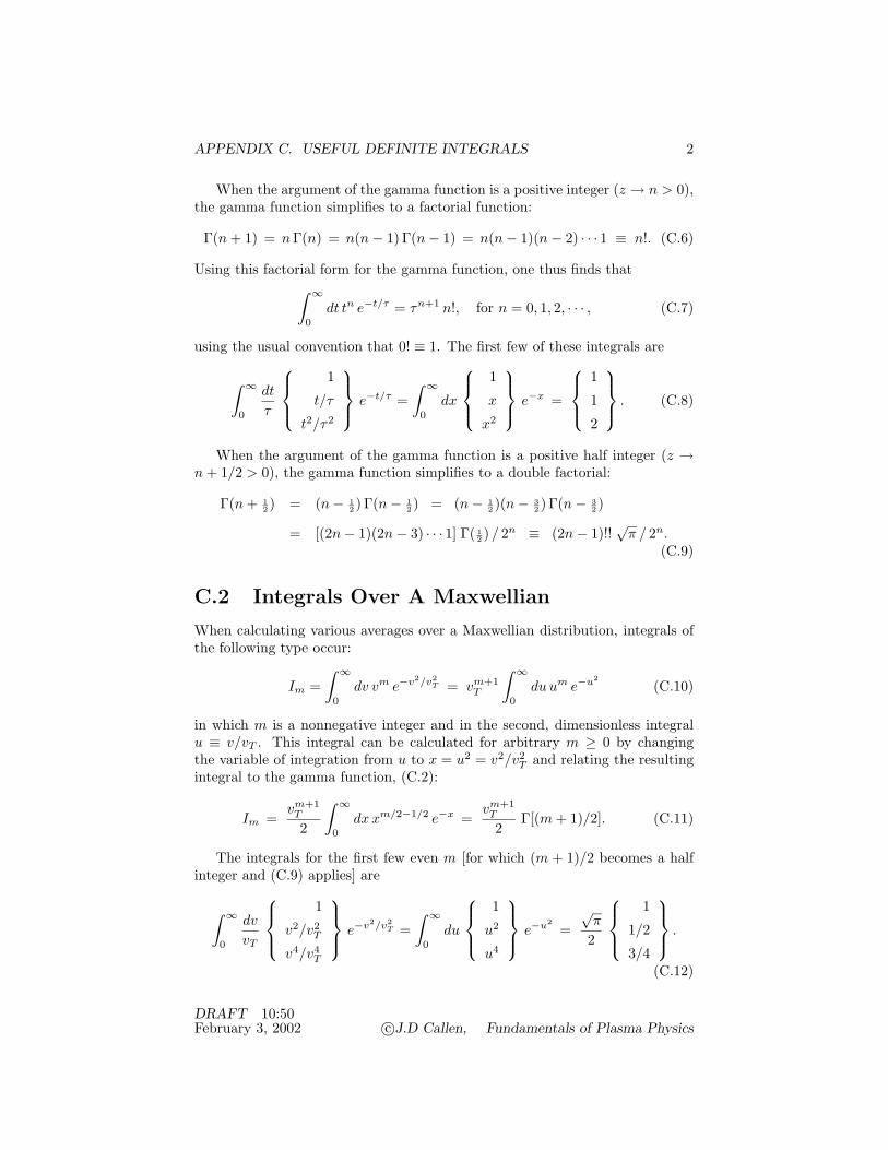
APPENDIX C. USEFUL DEFINITE INTEGRALS 2
When the argument of the gamma function is a positive integer (z → n > 0),the gamma function simplifies to a factorial function:
Γ(n + 1) = nΓ(n) = n(n − 1)Γ(n − 1) = n(n − 1)(n − 2) · · · 1 ≡ n!. (C.6)
Using this factorial form for the gamma function, one thus finds that∫ ∞
0dt tn e−t/τ = τn+1 n!, for n = 0, 1, 2, · · · , (C.7)
using the usual convention that 0! ≡ 1. The first few of these integrals are
∫ ∞
0
dt
τ
1
t/τ
t2/τ2
e−t/τ =∫ ∞
0dx
1
x
x2
e−x =
1
1
2
. (C.8)
When the argument of the gamma function is a positive half integer (z →n + 1/2 > 0), the gamma function simplifies to a double factorial:
Γ(n + 12 ) = (n − 1
2 )Γ(n − 12 ) = (n − 1
2 )(n − 32 )Γ(n − 3
2 )
= [(2n − 1)(2n − 3) · · · 1] Γ( 12 ) / 2n ≡ (2n − 1)!!
√π / 2n.
(C.9)
C.2 Integrals Over A Maxwellian
When calculating various averages over a Maxwellian distribution, integrals ofthe following type occur:
Im =∫ ∞
0dv vm e−v2/v2
T = vm+1T
∫ ∞
0du um e−u2
(C.10)
in which m is a nonnegative integer and in the second, dimensionless integralu ≡ v/vT . This integral can be calculated for arbitrary m ≥ 0 by changingthe variable of integration from u to x = u2 = v2/v2
T and relating the resultingintegral to the gamma function, (C.2):
Im =vm+1
T
2
∫ ∞
0dx xm/2−1/2 e−x =
vm+1T
2Γ[(m + 1)/2]. (C.11)
The integrals for the first few even m [for which (m + 1)/2 becomes a halfinteger and (C.9) applies] are
∫ ∞
0
dv
vT
1
v2/v2T
v4/v4T
e−v2/v2T =
∫ ∞
0du
1
u2
u4
e−u2=
√π
2
1
1/2
3/4
.
(C.12)
DRAFT 10:50February 3, 2002 c©J.D Callen, Fundamentals of Plasma Physics

APPENDIX C. USEFUL DEFINITE INTEGRALS 3
The integrals for the first few odd m [for which (m + 1)/2 becomes an integerand (C.6) applies] are
∫ ∞
0
dv
vT
v/vT
v3/v3T
v5/v5T
e−v2/v2T =
∫ ∞
0du
u
u3
u5
e−u2=
1/2
1/2
1
. (C.13)
The natural (orthogonal basis) energy weighting functions for expandingdistribution functions in terms of fluid moments are the Laguerre polynomialsLl+1/2
n (x), which are defined and discussed in Section B.6. The relevant di-mensionless integral of products of Laguerre polynomials that indicates theirorthogonality and normalization is∫ ∞
0dx xl+1/2 e−x L(l+1/2)
n (x) L(l+1/2)n′ (x)
= δnn′Γ(l + n + 3/2)Γ(n + 1)
= δnn′ [2(n + l) + 1]!!√
π
2n+l+1 n!
(C.14)
in which x ≡ v2/v2T = mv2/2T , and δnn′ is the Kronecker delta, which is unity
for n = n′ and vanishes if n (= n′. The lowest order (n = 0, 1, 2 and l = 0, 1, 2)integrals of interest are
∫ ∞
0dx x1/2e−x
[L(1/2)
0 ]2 [L1/21 ]2 [L1/2
2 ]2
x[L(3/2)0 ]2 x[L(3/2)
1 ]2 x[L(3/2)2 ]2
x2[L(5/2)0 ]2 x2[L(5/2)
1 ]2 x2[L(5/2)2 ]2
=√
π
2
1 3/2 15/4
3/2 15/4 105/8
15/8 105/16 945/32
.
(C.15)
C.3 Integrals Over Sinusoidal Functions
Averaging linear and nonlinear quantities made up of sinusoidally oscillatingcomponents result in integrals of the form
〈sinmϕ cosnϕ〉ϕ ≡ 12π
∫ 2π
0dϕ sinmϕ cosnϕ. (C.16)
Trigonometric identities that are useful in reducing these integrals to simplerforms are
2 sin ϕ cos ϕ = sin 2ϕ, (C.17)2 sin2ϕ = (1 − cos 2ϕ), (C.18)2 cos2ϕ = (1 + cos 2ϕ), (C.19)
DRAFT 10:50February 3, 2002 c©J.D Callen, Fundamentals of Plasma Physics
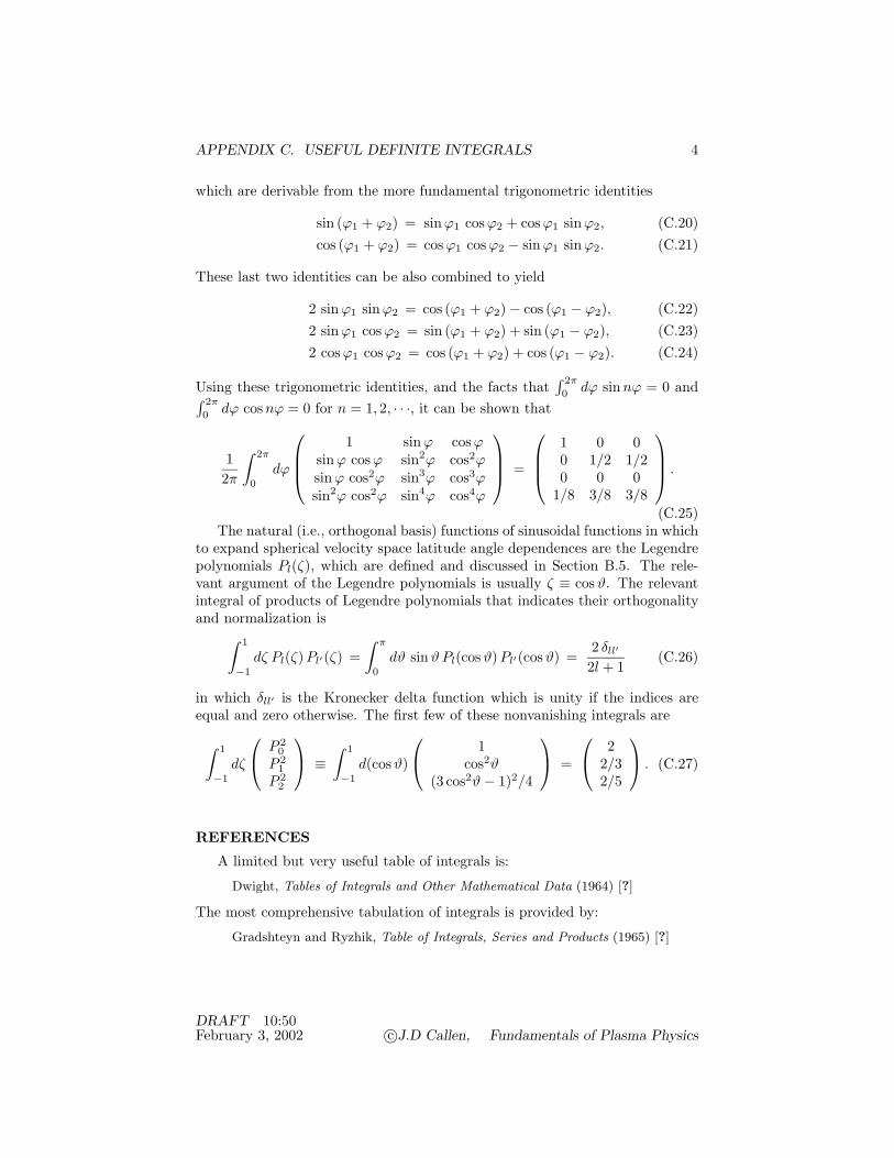
APPENDIX C. USEFUL DEFINITE INTEGRALS 4
which are derivable from the more fundamental trigonometric identities
sin (ϕ1 + ϕ2) = sinϕ1 cos ϕ2 + cos ϕ1 sinϕ2, (C.20)cos (ϕ1 + ϕ2) = cos ϕ1 cos ϕ2 − sinϕ1 sinϕ2. (C.21)
These last two identities can be also combined to yield
2 sin ϕ1 sinϕ2 = cos (ϕ1 + ϕ2) − cos (ϕ1 − ϕ2), (C.22)2 sin ϕ1 cos ϕ2 = sin (ϕ1 + ϕ2) + sin (ϕ1 − ϕ2), (C.23)2 cos ϕ1 cos ϕ2 = cos (ϕ1 + ϕ2) + cos (ϕ1 − ϕ2). (C.24)
Using these trigonometric identities, and the facts that∫ 2π0 dϕ sin nϕ = 0 and∫ 2π
0 dϕ cos nϕ = 0 for n = 1, 2, · · ·, it can be shown that
12π
∫ 2π
0dϕ
1 sinϕ cos ϕ
sinϕ cos ϕ sin2ϕ cos2ϕsinϕ cos2ϕ sin3ϕ cos3ϕsin2ϕ cos2ϕ sin4ϕ cos4ϕ
=
1 0 00 1/2 1/20 0 0
1/8 3/8 3/8
.
(C.25)The natural (i.e., orthogonal basis) functions of sinusoidal functions in which
to expand spherical velocity space latitude angle dependences are the Legendrepolynomials Pl(ζ), which are defined and discussed in Section B.5. The rele-vant argument of the Legendre polynomials is usually ζ ≡ cos ϑ. The relevantintegral of products of Legendre polynomials that indicates their orthogonalityand normalization is∫ 1
−1dζ Pl(ζ)Pl′(ζ) =
∫ π
0dϑ sinϑ Pl(cos ϑ)Pl′(cos ϑ) =
2 δll′
2l + 1(C.26)
in which δll′ is the Kronecker delta function which is unity if the indices areequal and zero otherwise. The first few of these nonvanishing integrals are
∫ 1
−1dζ
P 20
P 21
P 22
≡∫ 1
−1d(cos ϑ)
1cos2ϑ
(3 cos2ϑ − 1)2/4
=
22/32/5
. (C.27)
REFERENCES
A limited but very useful table of integrals is:
Dwight, Tables of Integrals and Other Mathematical Data (1964) [?]
The most comprehensive tabulation of integrals is provided by:
Gradshteyn and Ryzhik, Table of Integrals, Series and Products (1965) [?]
DRAFT 10:50February 3, 2002 c©J.D Callen, Fundamentals of Plasma Physics

APPENDIX D. VECTOR ANALYSIS 1
Appendix D
Vector Analysis
The following conventions are used in this appendix and throughout the book:
f, g,φ,ψ are scalar functions of x, t;A,B,C,D are vector functions of x, t;A = |A| ≡ √
A · A is the magnitude or length of the vector A;eA ≡ A/A is a unit vector in the A direction;x is the vector from the origin to the point (x, y, z);T,W, AB, etc., are dyad (second rank tensor) functions of x, t that will
be called simply tensors;I is the identity tensor or unit dyad;TT is the transpose of tensor T (interchange of indices of the tensor
elements), a tensor;tr(T) is the trace of the tensor T (sum of its diagonal elements), a scalar;det(T) ≡ ‖T‖ is the determinant of the tensor T (determinant of the
matrix of tensor elements), a scalar.
D.1 Vector Algebra
Basic algebraic relations:
A + B = B + A, commutative addition (D.1)A + (B + C) = (A + B) + C, associative addition (D.2)A − B = A + (−B), difference (D.3)fA = Af, commutative scalar multiplication (D.4)(f + g)A = fA + gA, distributive scalar multiplication (D.5)f(A + B) = fA + fB, distributive scalar multiplication (D.6)f(gA) = (fg)A, associative scalar multiplication (D.7)
DRAFT 11:26October 11, 2002 c©J.D Callen, Fundamentals of Plasma Physics
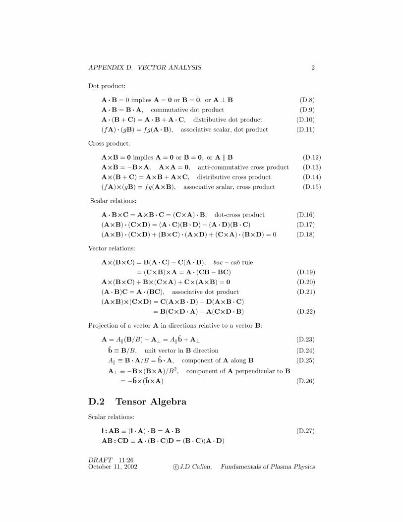
APPENDIX D. VECTOR ANALYSIS 2
Dot product:
A · B = 0 implies A = 0 or B = 0, or A ⊥ B (D.8)A · B = B · A, commutative dot product (D.9)A · (B + C) = A · B + A · C, distributive dot product (D.10)(fA) · (gB) = fg(A · B), associative scalar, dot product (D.11)
Cross product:
A×B = 0 implies A = 0 or B = 0, or A ‖ B (D.12)A×B = −B×A, A×A = 0, anti-commutative cross product (D.13)A×(B + C) = A×B + A×C, distributive cross product (D.14)(fA)×(gB) = fg(A×B), associative scalar, cross product (D.15)
Scalar relations:
A · B×C = A×B · C = (C×A) · B, dot-cross product (D.16)(A×B) · (C×D) = (A · C)(B · D) − (A · D)(B · C) (D.17)(A×B) · (C×D) + (B×C) · (A×D) + (C×A) · (B×D) = 0 (D.18)
Vector relations:
A×(B×C) = B(A · C) − C(A · B), bac − cab rule= (C×B)×A = A · (CB − BC) (D.19)
A×(B×C) + B×(C×A) + C×(A×B) = 0 (D.20)(A · B)C = A · (BC), associative dot product (D.21)(A×B)×(C×D) = C(A×B · D) − D(A×B · C)
= B(C×D · A) − A(C×D · B) (D.22)
Projection of a vector A in directions relative to a vector B:
A = A‖(B/B) + A⊥ = A‖b + A⊥ (D.23)
b ≡ B/B, unit vector in B direction (D.24)A‖ ≡ B · A/B = b · A, component of A along B (D.25)
A⊥ ≡ −B×(B×A)/B2, component of A perpendicular to B= −b×(b×A) (D.26)
D.2 Tensor Algebra
Scalar relations:
I : AB ≡ (I · A) · B = A · B (D.27)AB : CD ≡ A · (B · C)D = (B · C)(A · D)
DRAFT 11:26October 11, 2002 c©J.D Callen, Fundamentals of Plasma Physics

APPENDIX D. VECTOR ANALYSIS 3
dot!product cross!product
dot-cross!product
A
B
A
B
A
B
C
Figure D.1: Schematic illustration of dot, cross and dot-cross products of vec-tors.
DRAFT 11:26October 11, 2002 c©J.D Callen, Fundamentals of Plasma Physics
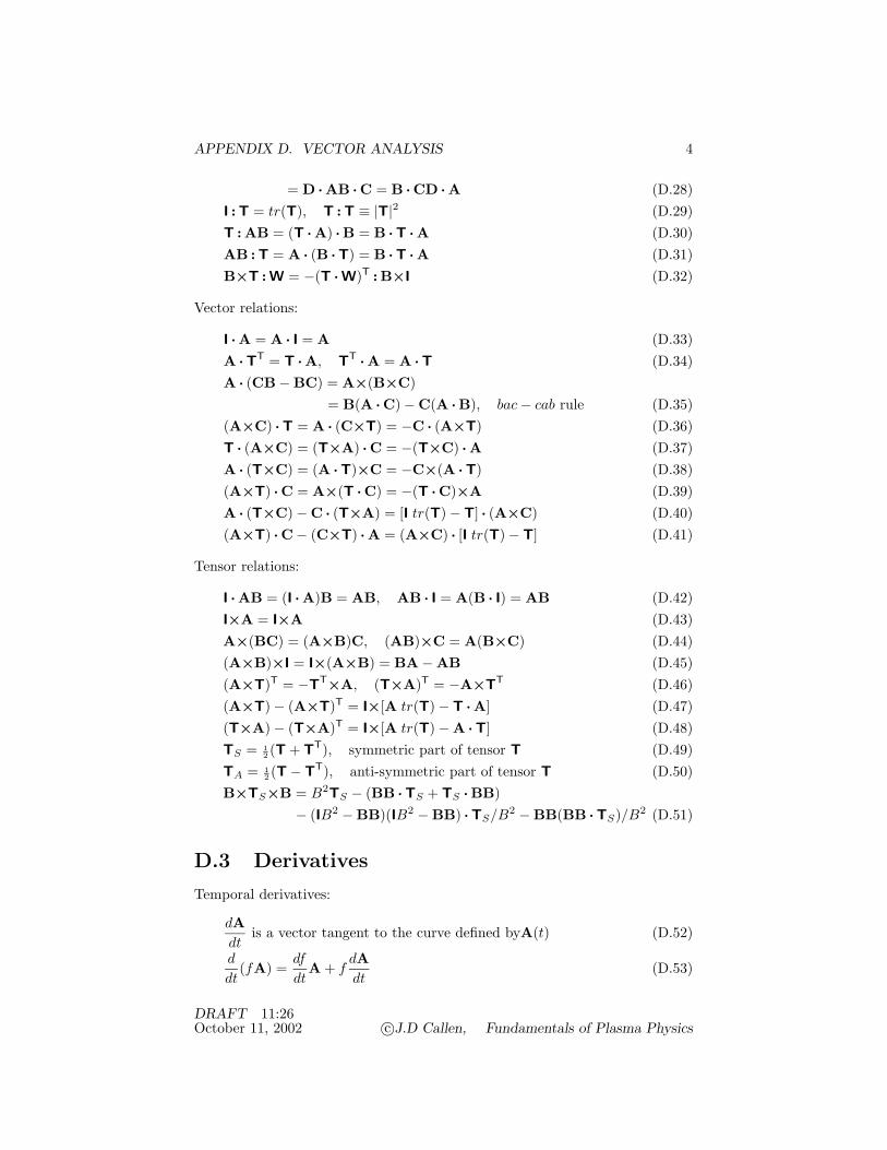
APPENDIX D. VECTOR ANALYSIS 4
= D · AB · C = B · CD · A (D.28)I : T = tr(T), T : T ≡ |T|2 (D.29)T : AB = (T · A) · B = B · T · A (D.30)AB : T = A · (B · T) = B · T · A (D.31)B×T : W = −(T · W)T : B×I (D.32)
Vector relations:
I · A = A · I = A (D.33)A · TT = T · A, TT · A = A · T (D.34)A · (CB − BC) = A×(B×C)
= B(A · C) − C(A · B), bac − cab rule (D.35)(A×C) · T = A · (C×T) = −C · (A×T) (D.36)T · (A×C) = (T×A) · C = −(T×C) · A (D.37)A · (T×C) = (A · T)×C = −C×(A · T) (D.38)(A×T) · C = A×(T · C) = −(T · C)×A (D.39)A · (T×C) − C · (T×A) = [I tr(T) − T] · (A×C) (D.40)(A×T) · C − (C×T) · A = (A×C) · [I tr(T) − T] (D.41)
Tensor relations:
I · AB = (I · A)B = AB, AB · I = A(B · I) = AB (D.42)I×A = I×A (D.43)A×(BC) = (A×B)C, (AB)×C = A(B×C) (D.44)(A×B)×I = I×(A×B) = BA − AB (D.45)(A×T)T = −TT×A, (T×A)T = −A×TT (D.46)(A×T) − (A×T)T = I×[A tr(T) − T · A] (D.47)(T×A) − (T×A)T = I×[A tr(T) − A · T] (D.48)TS = 1
2 (T + TT), symmetric part of tensor T (D.49)TA = 1
2 (T − TT), anti-symmetric part of tensor T (D.50)B×TS×B = B2TS − (BB · TS + TS · BB)
− (IB2 − BB)(IB2 − BB) · TS/B2 − BB(BB · TS)/B2 (D.51)
D.3 Derivatives
Temporal derivatives:
dAdt
is a vector tangent to the curve defined byA(t) (D.52)
d
dt(fA) =
df
dtA + f
dAdt
(D.53)
DRAFT 11:26October 11, 2002 c©J.D Callen, Fundamentals of Plasma Physics

APPENDIX D. VECTOR ANALYSIS 5
d
dt(A + B) =
dAdt
+dBdt
(D.54)
d
dt(A · B) =
dAdt
· B + A · dBdt
(D.55)
d
dt(A×B) =
dAdt
×B + A×dBdt
(D.56)
Definitions of partial derivatives in space (∇ ≡ ∂/∂x = del or nabla is thedifferential vector operator):
∇f ≡ ∂f
∂x, gradient of scalar function f , a vector — vector in direction
of and measure of the greatest rate of spatial change of f (D.57)
∇ · A ≡ ∂
∂x· A, divergence of vector function A, a scalar —
divergence (∇ · A > 0) or convergence (∇ · A < 0) of A lines (D.58)
∇×A ≡ ∂
∂x×A, curl (or rotation) of vector function A, a vector1—
vorticity of A lines (D.59)
∇2f ≡ ∇ · ∇f, del square or Laplacian (divergence of gradient)derivative of scalar function f , a scalar, which is sometimeswritten as ∆f — three-dimensional measure of curvature of f
(f is larger where ∇2f < 0 and smaller where ∇2f > 0) (D.60)
∇2A ≡ (∇ · ∇)A = ∇(∇ · A) − ∇×(∇×A), Laplacian derivativeof vector function A, a vector (D.61)
For the general vector coordinate x ≡ xex +yey +zez and |x| ≡ √x2 + y2 + z2:
∇ · x = 3, ∇ · (x/|x|) = 2/|x| (D.62)∇×x = 0, ∇×(x/|x|) = 0 (D.63)∇|x| = x/|x|, ∇(1/|x|) = −x/|x|3 (D.64)∇x = I (D.65)(A · ∇)(x/|x|) = [A − (x · A)x/|x|2]/|x| ≡ A⊥/|x| (D.66)∇2(1/|x|) ≡ ∇ · ∇(1/|x|) = −∇ · (x/|x|3) = −4πδ(x) (D.67)
1Rigorously speaking, the cross product of two vectors and the curl of a vector are pseudo-vectors because they are anti-symmetric contractions of second rank tensors — see tensorreferences at end of this appendix.
DRAFT 11:26October 11, 2002 c©J.D Callen, Fundamentals of Plasma Physics
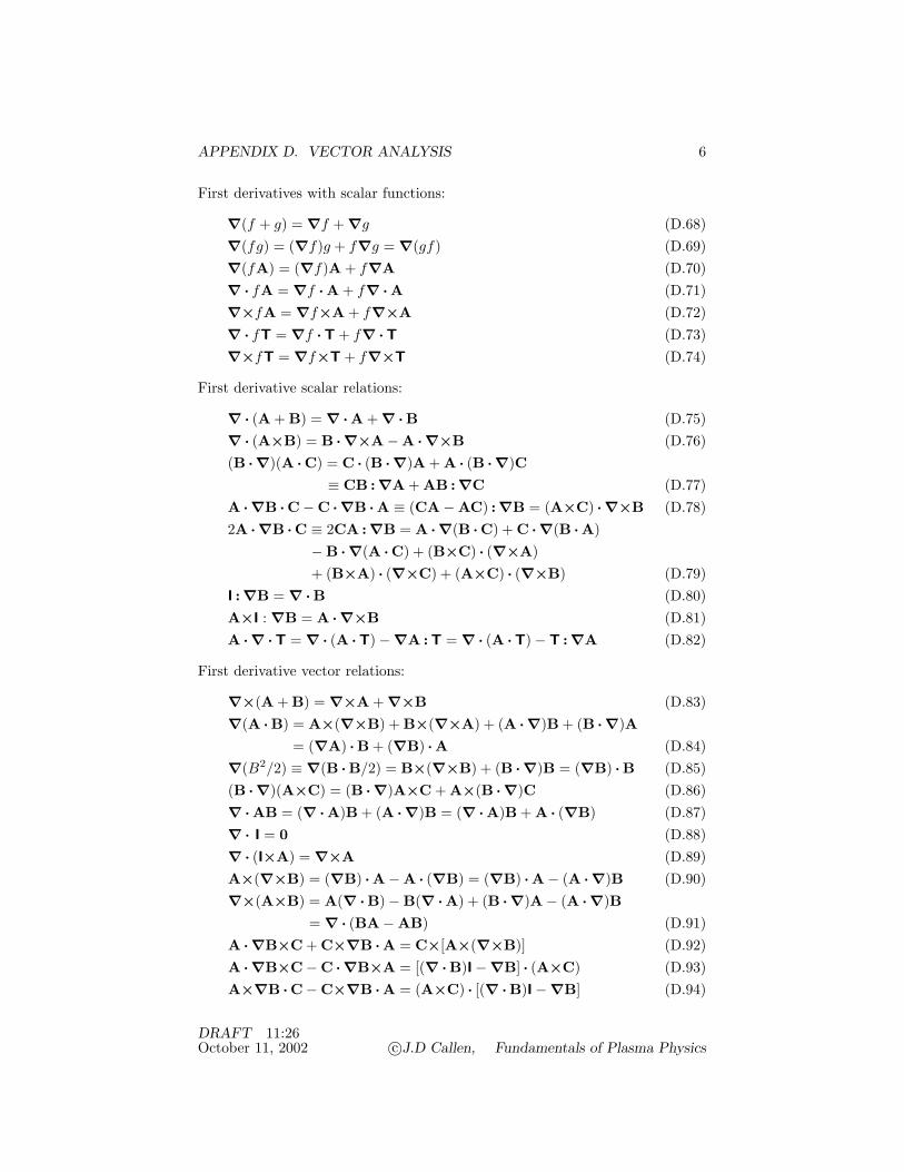
APPENDIX D. VECTOR ANALYSIS 6
First derivatives with scalar functions:
∇(f + g) = ∇f + ∇g (D.68)∇(fg) = (∇f)g + f∇g = ∇(gf) (D.69)∇(fA) = (∇f)A + f∇A (D.70)∇ · fA = ∇f · A + f∇ · A (D.71)∇×fA = ∇f×A + f∇×A (D.72)∇ · fT = ∇f · T + f∇ · T (D.73)∇×fT = ∇f×T + f∇×T (D.74)
First derivative scalar relations:
∇ · (A + B) = ∇ · A + ∇ · B (D.75)∇ · (A×B) = B · ∇×A − A · ∇×B (D.76)(B · ∇)(A · C) = C · (B · ∇)A + A · (B · ∇)C
≡ CB : ∇A + AB : ∇C (D.77)A · ∇B · C − C · ∇B · A ≡ (CA − AC) : ∇B = (A×C) · ∇×B (D.78)2A · ∇B · C ≡ 2CA : ∇B = A · ∇(B · C) + C · ∇(B · A)
− B · ∇(A · C) + (B×C) · (∇×A)+ (B×A) · (∇×C) + (A×C) · (∇×B) (D.79)
I : ∇B = ∇ · B (D.80)A×I : ∇B = A · ∇×B (D.81)A · ∇ · T = ∇ · (A · T) − ∇A : T = ∇ · (A · T) − T : ∇A (D.82)
First derivative vector relations:
∇×(A + B) = ∇×A + ∇×B (D.83)∇(A · B) = A×(∇×B) + B×(∇×A) + (A · ∇)B + (B · ∇)A
= (∇A) · B + (∇B) · A (D.84)∇(B2/2) ≡ ∇(B · B/2) = B×(∇×B) + (B · ∇)B = (∇B) · B (D.85)(B · ∇)(A×C) = (B · ∇)A×C + A×(B · ∇)C (D.86)∇ · AB = (∇ · A)B + (A · ∇)B = (∇ · A)B + A · (∇B) (D.87)∇ · I = 0 (D.88)∇ · (I×A) = ∇×A (D.89)A×(∇×B) = (∇B) · A − A · (∇B) = (∇B) · A − (A · ∇)B (D.90)∇×(A×B) = A(∇ · B) − B(∇ · A) + (B · ∇)A − (A · ∇)B
= ∇ · (BA − AB) (D.91)A · ∇B×C + C×∇B · A = C×[A×(∇×B)] (D.92)A · ∇B×C − C · ∇B×A = [(∇ · B)I − ∇B] · (A×C) (D.93)A×∇B · C − C×∇B · A = (A×C) · [(∇ · B)I − ∇B] (D.94)
DRAFT 11:26October 11, 2002 c©J.D Callen, Fundamentals of Plasma Physics

APPENDIX D. VECTOR ANALYSIS 7
First derivative tensor relations:
I · ∇B = ∇B, ∇B · I = ∇B (D.95)∇×AB = (∇×A)B − A×∇B (D.96)∇(A×B) = ∇A×B − ∇B×A (D.97)A×∇B + ∇B×A
= I×[(∇ · B)A − (∇B) · A] + [A · (∇×B)]I − A(∇×B)= I×[(∇ · B)A − A · (∇B)] + [A · (∇×B)]I − (∇×B)A (D.98)
∇B×A + (A×∇B)T = [A · (∇×B)]I − A(∇×B) (D.99)A×∇B + (∇B×A)T = [A · (∇×B)]I − (∇×B)A (D.100)A×∇B − (A×∇B)T = I×[(∇ · B)A − (∇B) · A] (D.101)∇B×A − (∇B×A)T = [(∇ · B)A − A · (∇B)]×I (D.102)
Second derivative relations:
∇ · ∇f ≡ ∇2f (D.103)∇×∇f = 0 (D.104)∇ · ∇f×∇g = 0 (D.105)∇ · ∇A ≡ ∇2A = ∇(∇ · A) − ∇×(∇×A) (D.106)∇ · ∇×A = 0 (D.107)∇ · (B · ∇)A = (B · ∇)(∇ · A) − (∇×A) · (∇×B) (D.108)∇×[(A · ∇)A]
= (A · ∇)(∇×A) + (∇ · A)(∇×A) − [(∇×A) · ∇]A (D.109)
Derivatives of projections of A in B direction [b ≡ B/B, A = A‖b + A⊥,A‖ ≡ b · A, A⊥ ≡ − b×(b×A), (b · ∇)b = − b×(∇×b) ≡ κ]:
∇ · A = (A‖/B)(∇ · B) + (B · ∇)(A‖/B) + ∇ · A⊥ (D.110)
∇ · A⊥ = −A⊥ · [ ∇ lnB + (b · ∇)b ] − (1/B) b · ∇×(B×A) (D.111)b · ∇A · b ≡ bb : ∇A = (b · ∇)A‖ − A⊥ · (b · ∇)b
= A · ∇ lnB − (1/B)b · ∇×(B×A) + ∇ · A − (A‖/B)(∇ · B) (D.112)
For A⊥ = (1/B2)B×∇f, b · ∇×(B×A⊥) = (b · ∇f)(b · ∇×b) (D.113)
D.4 Integrals
For a volume V enclosed by a closed, continuous surface S with differentialvolume element d3x and differential surface element dS ≡ n dS where n is theunit normal outward from the volume V , for well-behaved functions f, g,A,Band T:∫
Vd3x∇f =
∫©∫
SdS f, (D.114)
DRAFT 11:26October 11, 2002 c©J.D Callen, Fundamentals of Plasma Physics
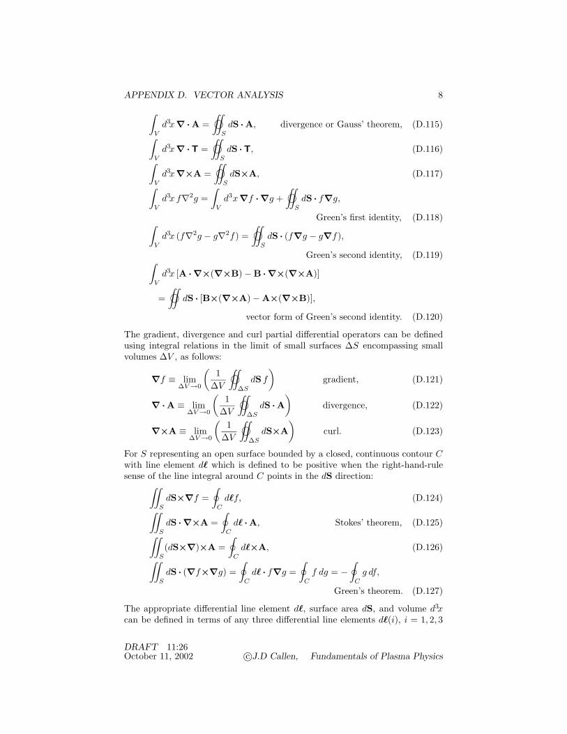
APPENDIX D. VECTOR ANALYSIS 8∫V
d3x∇ · A =∫©∫
SdS · A, divergence or Gauss’ theorem, (D.115)∫
Vd3x∇ · T =
∫©∫
SdS · T, (D.116)∫
Vd3x∇×A =
∫©∫
SdS×A, (D.117)∫
Vd3x f∇2g =
∫V
d3x∇f · ∇g +∫©∫
SdS · f∇g,
Green’s first identity, (D.118)∫V
d3x (f∇2g − g∇2f) =∫©∫
SdS · (f∇g − g∇f),
Green’s second identity, (D.119)∫V
d3x [A · ∇×(∇×B) − B · ∇×(∇×A)]
=∫©∫
dS · [B×(∇×A) − A×(∇×B)],
vector form of Green’s second identity. (D.120)
The gradient, divergence and curl partial differential operators can be definedusing integral relations in the limit of small surfaces ∆S encompassing smallvolumes ∆V , as follows:
∇f ≡ lim∆V →0
(1∆V
∫©∫
∆SdS f
)gradient, (D.121)
∇ · A ≡ lim∆V →0
(1∆V
∫©∫
∆SdS · A
)divergence, (D.122)
∇×A ≡ lim∆V →0
(1∆V
∫©∫
∆SdS×A
)curl. (D.123)
For S representing an open surface bounded by a closed, continuous contour Cwith line element d" which is defined to be positive when the right-hand-rulesense of the line integral around C points in the dS direction:∫∫
SdS×∇f =
∮C
d"f, (D.124)∫∫S
dS · ∇×A =∮
Cd" · A, Stokes’ theorem, (D.125)∫∫
S(dS×∇)×A =
∮C
d"×A, (D.126)∫∫S
dS · (∇f×∇g) =∮
Cd" · f∇g =
∮C
f dg = −∮
Cg df,
Green’s theorem. (D.127)
The appropriate differential line element d", surface area dS, and volume d3xcan be defined in terms of any three differential line elements d"(i), i = 1, 2, 3
DRAFT 11:26October 11, 2002 c©J.D Callen, Fundamentals of Plasma Physics
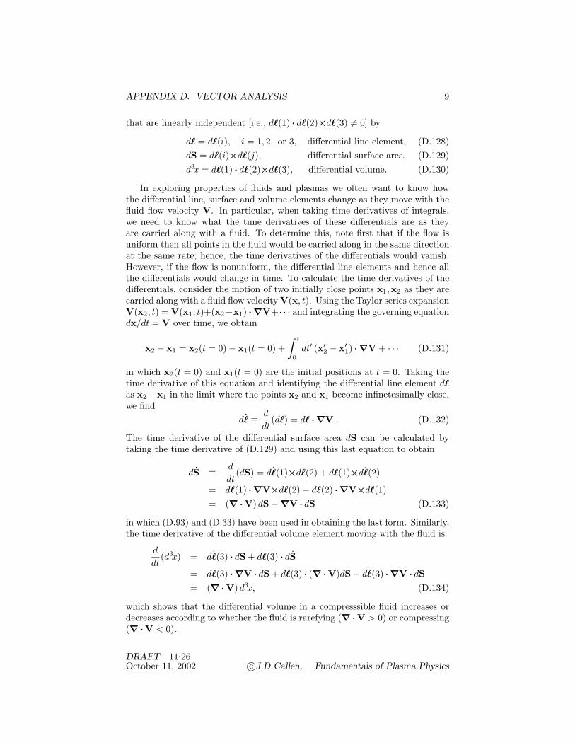
APPENDIX D. VECTOR ANALYSIS 9
that are linearly independent [i.e., d"(1) · d"(2)×d"(3) (= 0] by
d" = d"(i), i = 1, 2, or 3, differential line element, (D.128)dS = d"(i)×d"(j), differential surface area, (D.129)d3x = d"(1) · d"(2)×d"(3), differential volume. (D.130)
In exploring properties of fluids and plasmas we often want to know howthe differential line, surface and volume elements change as they move with thefluid flow velocity V. In particular, when taking time derivatives of integrals,we need to know what the time derivatives of these differentials are as theyare carried along with a fluid. To determine this, note first that if the flow isuniform then all points in the fluid would be carried along in the same directionat the same rate; hence, the time derivatives of the differentials would vanish.However, if the flow is nonuniform, the differential line elements and hence allthe differentials would change in time. To calculate the time derivatives of thedifferentials, consider the motion of two initially close points x1,x2 as they arecarried along with a fluid flow velocity V(x, t). Using the Taylor series expansionV(x2, t) = V(x1, t)+(x2−x1) · ∇V+· · · and integrating the governing equationdx/dt = V over time, we obtain
x2 − x1 = x2(t = 0) − x1(t = 0) +∫ t
0dt′ (x′
2 − x′1) · ∇V + · · · (D.131)
in which x2(t = 0) and x1(t = 0) are the initial positions at t = 0. Taking thetime derivative of this equation and identifying the differential line element d"as x2 −x1 in the limit where the points x2 and x1 become infinetesimally close,we find
d" ≡ d
dt(d") = d" · ∇V. (D.132)
The time derivative of the differential surface area dS can be calculated bytaking the time derivative of (D.129) and using this last equation to obtain
dS ≡ d
dt(dS) = d"(1)×d"(2) + d"(1)×d"(2)
= d"(1) · ∇V×d"(2) − d"(2) · ∇V×d"(1)= (∇ · V) dS − ∇V · dS (D.133)
in which (D.93) and (D.33) have been used in obtaining the last form. Similarly,the time derivative of the differential volume element moving with the fluid is
d
dt(d3x) = d"(3) · dS + d"(3) · dS
= d"(3) · ∇V · dS + d"(3) · (∇ · V)dS − d"(3) · ∇V · dS= (∇ · V) d3x, (D.134)
which shows that the differential volume in a compresssible fluid increases ordecreases according to whether the fluid is rarefying (∇ · V > 0) or compressing(∇ · V < 0).
DRAFT 11:26October 11, 2002 c©J.D Callen, Fundamentals of Plasma Physics

APPENDIX D. VECTOR ANALYSIS 10
D.5 Vector Field Representations
Any vector field B can be expressed in terms of a scalar potential ΦM and avector potential A:
B = −∇ΦM + ∇×A, potential representation. (D.135)
The ∇ΦM part of B represents the longitudinal or irrotational (∇×∇ΦM = 0)component while the ∇×A part represents the transverse or solenoidal compo-nent (∇ · ∇×A = 0). A vector field B that satisfies ∇×B = 0 is called a lon-gitudinal or irrotational field; one that satisfies ∇ · B = 0 is called a solenoidalor transverse field. For a B(x) that vanishes at infinity, the potentials ΦM andA are given by Green’s function solutions
ΦM (x) =∫
d3x′ (∇ · B)x′
4π|x − x′| , A(x) =∫
d3x′ (∇×B)x′
4π|x − x′| . (D.136)
When there is symmetry in a coordinate ζ (i.e., a two or less dimensionalsystem), a solenoidal vector field B can be written in terms of a stream functionψ in such a way that it automatically satisfies the solenoidal condition ∇ · B = 0:
B = ∇ζ×∇ψ = |∇ζ| eζ×∇ψ = −∇×ψ∇ζ, stream function form.(D.137)
For this situation the vector potential becomes
A = −ψ ∇ζ = −ψ |∇ζ| eζ . (D.138)
For a fully three-dimensional situation with no symmetry, a solenoidal vectorfield B can in general be written as
B = ∇α×∇β, Clebsch representation, (D.139)
In this representation α and β are stream functions that are constant along thevector field B since B · ∇α = 0 and B · ∇β = 0.
D.6 Properties Of Curve Along A Vector Field
The motion of a point x along a vector field B is described by
dxd)
=BB
= b ≡ T, tangent vector (D.140)
in which d) is a differential distance along B. The unit vector b is tangent tothe vector field B(x) at the point x and so is often written as T — a unit tangentvector.
The curvature vector κ of the vector field B is defined by
κ ≡ d2xd)2
=dbd)
= (b · ∇)b = − b×(∇×b), curvature vector (D.141)
DRAFT 11:26October 11, 2002 c©J.D Callen, Fundamentals of Plasma Physics

APPENDIX D. VECTOR ANALYSIS 11
in which (D.85) has been used in the obtaining the last expression. The unitvector in the curvature vector direction is defined by
κ ≡ (b · ∇)b / |(b · ∇)b|, curvature unit vector. (D.142)
The local radius of curvature vector RC is in the opposite direction from thecurvature vector κ and is defined by
RC ≡ −κ/|κ|2, κ = −RC/R2C , radius of curvature. (D.143)
Hence, |RC | ≡ RC = 1/|κ| is the magnitude of the local radius of curvature —the radius of the circle tangent to the vector field B(x) at the point x.
A triad of orthogonal unit vectors (see Fig. D.2) can be constructed from thetangent unit vector T and an arbitrary unit vector N normal (or perpendicular)to the vector field B(x) at the point x:
T ≡ b, N and B ≡ T×N = b×N, Frenet unit vector triad (D.144)
in which B is the binormal unit vector, the third orthogonal unit vector. Thecomponent of a vector C in the direction of the vector field B is called theparallel component: C‖ ≡ T · C = b · C. The component in the N direction iscalled the normal component: CN ≡ N · C. The component in the B direction,which is perpendicular to the T×N plane, is called the binormal component:CB ≡ B · C = T×N · C.
Consider for example the components of the curvature vector κ. Sinceb · κ = 0, the curvature vector has no parallel component (κ‖ = 0) — thecurvature vector for the vector field B(x) is perpendicular to it at the pointx. The components of the curvature vector κ relative to a surface ψ(x) = con-stant in which the vector field lies (i.e., B · ∇ψ = 0) can be specified as follows.Define the normal to be in the direction of the gradient of ψ: N ≡ ∇ψ/|∇ψ|.Then, the components of the curvature vector perpendicular to (normal) andlying within (geodesic) the ψ surface are given by
κn = N · κ = ∇ψ · κ/|∇ψ|, normal curvature, (D.145)
κg = B · κ = (b×∇ψ) · κ/|b×∇ψ|, geodesic curvature. (D.146)
The torsion τ (twisting) of a vector field B is defined by
τ ≡ − dB
d)= − (b · ∇)(b×N), torsion vector. (D.147)
The binormal component of the torsion vector vanishes (τB ≡ B · τ = 0). Thenormal component of the torsion vector locally defines the scale length Lτ alongthe vector B over which the vector field B(x) twists through an angle of oneradian:
Lτ ≡ 1/|τN|, τN ≡ − N · dB
d)= − N · (b · ∇)(b×N), torsion length. (D.148)
DRAFT 11:26October 11, 2002 c©J.D Callen, Fundamentals of Plasma Physics

APPENDIX D. VECTOR ANALYSIS 12
B
B
B
curvature torsion
shear
Rc
Figure D.2: Properties (curvature, torsion, shear) of a spatially inhomogeneousvector field B(x). The unit vector b ≡ B/B = dx/d) = T is locally tangent tothe vector field B. The unit normal N is perpendicular to the vector field B,shown here in the curvature direction. The binormal B is orthogonal to both band N.
DRAFT 11:26October 11, 2002 c©J.D Callen, Fundamentals of Plasma Physics

APPENDIX D. VECTOR ANALYSIS 13
If the unit normal N is taken to be in the ∇ψ direction, the parallel com-ponent of the torsion vector is equal to the geodesic curvature [τ‖ ≡ b · τ =(b×∇ψ) · (b · ∇)b / |b×∇ψ| ≡ κg].
The local shear ς (differential twisting motion, or nonplanar differential tan-gential motion in the plane defined by b = T and N) in a vector field B is givenby the binormal component of the curl or rotation in the binormal unit vector:
ς ≡ B · ∇×B = (b×N) · ∇×(b×N) ≡ 1/LS , local shear. (D.149)
The shear length LS is defined as the scale length over which the vector fieldB(x) shears through an angle of one radian. The parallel component of thetotal curl or rotation of a vector field B is given by a combination of its torsionand shear, and N · ∇×N:
σ ≡ b · ∇×b = (b×N) · ∇×(b×N) − 2N · (b · ∇)(b×N) + N · ∇×N
= ς + 2τN + N · ∇×N, total rotation in B field. (D.150)
If the normal N is taken to be in the ∇ψ direction, N · ∇×N = 0 and then
ς =(b×∇ψ) · ∇×(b×∇ψ)
|b×∇ψ|2 ≡ 1LS
, local shear with N ≡ ∇ψ/|∇ψ|,(D.151)
andσ ≡ b · ∇×b = ς + 2τN. (D.152)
In the absence of shear (ς = 0), this last relation yields τN = (1/2)b · ∇×b —the torsion for “rigid body rotation” is just half the parallel component of therotation in the vector field B.
In most applied mathematics books the normal N is taken to be in the curva-ture vector direction (i.e., N ≡ κ) instead of the ∇ψ direction. Then, the parallelcomponent of the torsion vector also vanishes [τ‖ ≡ b · τ = b×κ · (b · ∇)b =b×κ · κ = 0] and
τ ≡ τNN, for N ≡ κ. (D.153)
For this case the interrelationships between the triad of unit vectors T, N, B aregiven by the Frenet-Serret formulas:
dT
d)= κNN, T ≡ B/B ≡ b,
dN
d)= −κNT + τNB, N ≡ κ = (b · ∇)b / |(b · ∇)b|,
dB
d)= −τNN, B ≡ T×N = b×κ.
(D.154)
The local shear ς and total rotation σ in the vector field B for this case are asgiven above in (D.149) and (D.150), respectively, for a general unit normal N.
DRAFT 11:26October 11, 2002 c©J.D Callen, Fundamentals of Plasma Physics

APPENDIX D. VECTOR ANALYSIS 14
D.7 Base Vectors and Vector Components
The three vectors e1, e2, e3, which are not necessarily orthogonal, can be used asa basis for a three-dimensional coordinate system if they are linearly independent(i.e., e1 · e2×e2 (= 0). The three reciprocal base vectors e1, e2, e3 are defined by
ei · ej = δij , (D.155)
whereδij ≡
1, i = j,0, i (= j,
Kronecker delta. (D.156)
The reciprocal base vectors can be written in terms of the original base vectors:
e1 =e2×e3
e1 · (e2×e3), e2 =
e3×e1
e1 · (e2×e3), e3 =
e1×e2
e1 · (e2×e3). (D.157)
Or, in general index notation
ei = εijkej×ek
e1 · (e2×e3), i, j, k = permutations of 1, 2, 3 (D.158)
in which
εijk =
+1 when i, j, k is an even permutation of 1, 2, 3−1 when i, j, k is an odd permutation of 1, 2, 3
0 when any two indices are equal Levi-Civita symbol.(D.159)
The reciprocal Levi–Civita symbol εijk is the same, i.e., εijk=εijk. These for-mulas are also valid if the subscripts and subscripts are reversed. Thus, the“original” base vectors could be the reciprocal base vectors ei and the “recip-rocal” base vectors could be the original base vectors ei since both sets of basevectors are linearly independent. Either set can be used as a basis for repre-senting three-dimensional vectors.
The identity tensor can be written in terms of the base or reciprocal vectorsas follows:
I ≡ ∑i e
iei = e1e1 + e2e2 + e3e3
≡ ∑i eiei = e1e1 + e2e2 + e3e3.
identity tensor (D.160)
This definition can be used to write any vector or operator in terms of eitherits base or reciprocal vector components:
A = A · I = (A · e1)e1 + (A · e2)e2 + (A · e3)e3 =∑
i
Aiei, Ai ≡ A · ei,
= (A · e1)e1 + (A · e2)e2 + (A · e3)e3 =∑
j
Ajej , Aj ≡ A · ej ,
(D.161)∇ ≡ I · ∇ = e1(e1 · ∇) + e2(e2 · ∇) + e3(e3 · ∇)
= e1(e1 · ∇) + e2(e2 · ∇) + e3(e3 · ∇). (D.162)
DRAFT 11:26October 11, 2002 c©J.D Callen, Fundamentals of Plasma Physics

APPENDIX D. VECTOR ANALYSIS 15
The dot product between two vectors A and B is given in terms of theirbase and reciprocal vector components by
A · B =∑
i
AiBi =∑
i
AiBi =
∑ij
(ei · ej)AiBj =∑ij
(ei · ej)AiBj . (D.163)
Similarly, the cross product between two vectors is given by
A×B =∑ij
AiBj ei×ej =∑ijk
AiBj ek (e1 · e2×e3)
=∑ij
AiBj ei×ej =∑ijk
εijkAiBj ek (e1 · e2×e3)
= (e1 · e2×e3)
∥∥∥∥∥∥e1 e2 e3
A1 A2 A3
B1 B2 B3
∥∥∥∥∥∥ = (e1 · e2×e3)
∥∥∥∥∥∥e1 e2 e3
A1 A2 A3
B1 B2 B3
∥∥∥∥∥∥ . (D.164)
The dot-cross product of three vectors is given by
A · B×C =∑ijk
AiBjCk ei · ej×ek =∑ijk
εijkAiBjCk (e1 · e2×e3)
=∑ijk
AiBjCk ei · ej×ek =∑ijk
εijkAiBjCk (e1 · e2×e3)
= (e1 · e2×e3)
∥∥∥∥∥∥A1 A2 A3
B1 B2 B3
C1 C2 C3
∥∥∥∥∥∥ = (e1 · e2×e3)
∥∥∥∥∥∥A1 A2 A3
B1 B2 B3
C1 C2 C3
∥∥∥∥∥∥ . (D.165)
For the simplest situation where the three base vectors e1, e2, e3 are orthog-onal (e1 · e2 = e2 · e3 = e1 · e3 = 0), the reciprocal vectors point in the samedirections as the original base vectors. Thus, after normalizing the base andreciprocal vectors they become equal:
e1 = e1/|e1| = e1 = e1/|e1| orthogonale2 = e2/|e2| = e2 = e2/|e2| unite3 = e3/|e3| = e3 = e3/|e3| vectors. (D.166)
The simplifications of (??)–(??) are given in (D.196)–(D.201) in the section(D.9) below on orthogonal coordinate systems.
D.8 Curvilinear Coordinate Systems
Consider transformation from the Cartesian coordinate system x = (x, y, z)to a curvilinear coordinate system labeled by the three independent functionsu1, u2, u3:
x = x(u1, u2, u3) : x = x(u1, u2, u3), y = y(u1, u2, u3), z = z(u1, u2, u3).(D.167)
DRAFT 11:26October 11, 2002 c©J.D Callen, Fundamentals of Plasma Physics

APPENDIX D. VECTOR ANALYSIS 16
The transformation is invertible if the partial derivatives ∂x/∂ui for i = 1, 2, 3are continuous and the Jacobian determinant (i.e., ∂x/∂u1 · ∂x/∂u2×∂x/∂u3)formed from these nine partial derivatives does not vanish in the domain ofinterest. The inverse transformation is then given by
ui = ui(x) : u1 = u1(x, y, z), u2 = u2(x, y, z), u3 = u3(x, y, z). (D.168)
In a curvilinear coordinate system there are three coordinate surfaces:
u1(x) = c1 (u2, u3 variable),u2(x) = c2 (u1, u3 variable),u3(x) = c3 (u1, u2 variable).
(D.169)
There are also three coordinate curves given by
u2(x) = c2, u3(x) = c3 (u1 variable),u3(x) = c3, u1(x) = c1 (u2 variable),u1(x) = c1, u2(x) = c2 (u3 variable).
(D.170)
The direction in which ui increases along a coordinate curve is taken to be thepositive direction for ui. If the curvilinear coordinate curves intersect at rightangles (i.e., ∇ui · ∇uj = 0 except for i = j), then the system is orthogonal. Thefamiliar Cartesian, cylindrical and spherical coordinate systems are all orthogo-nal. They are discussed at the end of the next section which covers orthogonalcoordinates.
A nonorthogonal curvilinear coordinate system can be constructed from aninvertible set of functions u1(x), u2(x), u3(x) as follows. A set of base vectorsei can be defined by
ei = ∇ui, i = 1, 2, 3 contravariant base vectors. (D.171)
These so-called contravariant (superscript index) base vectors point in the direc-tion of the gradient of the curvilinear coordinates ui, and hence in the directionsperpendicular to the ui(x) = ci surfaces. The set of reciprocal base vectors ei
is given by
ei = εijkej×ek
e1 · e2×e3=
εijk
J−1∇uj×∇uk, covariant base vectors, (D.172)
in which
J−1 ≡ ∇u1 · ∇u2×∇u3 = e1 · e2×e3 inverse Jacobian (D.173)
is the Jacobian of the “inverse” transformation from the ui curvilinear coordi-nate system back to the original Cartesian coordinate system.
An alternative form for the reciprocal base vectors can be obtained from thedefinition of the derivative of one of the curvilinear coordinates ui(x) in termsof the gradient: dui = ∇ui · dx = ∇ui · ∑
j(∂x/∂uj) dxj , which becomes an
DRAFT 11:26October 11, 2002 c©J.D Callen, Fundamentals of Plasma Physics

APPENDIX D. VECTOR ANALYSIS 17
identity if and only if ∇ui · (∂x/∂uj) = δij . Since this last relation is the same
as the defining relation for reciprocal base vectors (ei · ej = δij), it follows that
ei =∂x∂ui
, i = 1, 2, 3 covariant base vectors. (D.174)
The so-called covariant (subscript index) base vectors point in the directionof the local tangent to the ui variable coordinate curve (from the ∂x/∂ui def-inition), i.e., parallel to the ui coordinate curve. Alternatively, the covariantbase vectors can be thought of as pointing in the direction of the cross productof contravariant base vectors for the two coordinate surfaces other than the ui
coordinate being considered (from the ∇uj×∇uk definition). That these twodirectional definitions coincide follows from the properties of curvilinear sur-faces and curves. The contravariant base vectors ei can also be defined as thereciprocal base vectors of covariant base vectors ei:
ei = εijk ej×ek
e1 · e2×e2=
εijk
J
∂x∂uj
× ∂x∂uk
; i, j, k = permutations of 1, 2, 3
contravariant base vectors(D.175)
in whichJ =
∂x∂u1
· ∂x∂u2
× ∂x∂u3
= e1 · e2×e3 Jacobian (D.176)
is the Jacobian of the transformation from the Cartesian coordinate system tothe curvilinear coordinate system specified by the functions ui.
The geometrical properties of a nonorthogonal curvilinear coordinate systemare characterized by the dot products of the base vectors:
gij ≡ ei · ej =∂x∂ui
· ∂x∂uj
covariant metric elements,
gij ≡ ei · ej = ∇ui · ∇uj contravariant metric elements.(D.177)
These symmetric tensor metric elements can be used to write the covariantcomponents of a vector in terms of its contravariant components and vice versa:
Ai ≡ A · ei = A · I · ei =∑
j
(A · ej)(ej · ei) =∑
j
gij Aj
Ai ≡ A · ei = A · I · ei =∑
j
(A · ej)(ej · ei) =∑
j
gijAi.(D.178)
Similarly, they can also be used to write the covariant base vectors in terms ofthe contravariant base vectors and vice versa:
ei =∑
j
gij ej , ei =∑
j
gij ei. (D.179)
From the dot product between these relations and their respective reciprocalbase vectors it can be shown that∑
j
gij gjk =∑
j
gkjgji = δki . (D.180)
DRAFT 11:26October 11, 2002 c©J.D Callen, Fundamentals of Plasma Physics

APPENDIX D. VECTOR ANALYSIS 18
The determinant of the matrix comprised of the metric coefficients is calledg:
g ≡ ‖gij‖ =∥∥gij
∥∥−1, (D.181)
in which the second relation follows from interpreting the summation relationsat the end of the preceding paragraph in terms of matrix operations: [gij ][gik]= [I], which yields [gij ] = [gjk]−1. Since the determinant of the inner productof two matrices is given by the product of the determinants of the two matrices,
g = ‖gij‖ =∥∥∥∥ ∂x∂ui
· ∂x∂uj
∥∥∥∥ =∥∥∥∥ ∂x∂ui
∥∥∥∥∥∥∥∥ ∂x∂uj
∥∥∥∥ =(
∂x∂u1
· ∂x∂u2
× ∂x∂u3
)2
= J2.
(D.182)Thus, the determinant of the metric coefficients is related to the Jacobian andinverse Jacobian as follows:
J =√
g = e1 · e2×e3 =∂x∂u1
· ∂x∂u2
× ∂x∂u3
Jacobian,
J−1 = 1/√
g = e1 · e2×e3 = ∇u1 · ∇u2×∇u3 inverse Jacobian.(D.183)
The various partial derivatives in space can be worked out in terms of covari-ant derivatives (∂/∂ui) using the properties of the covariant and contravariantbase vectors for a general, nonorthogonal curvilinear coordinate system as fol-lows:
∇f =∑
i
∇ui ∂f
∂ui=
∑i
ei ∂f
∂uigradient,
(D.184)
∇ · A = ∇ · (A · I) = ∇ ·∑
i
√g (A · ei)
ei√g
=∑
i
ei√g
· ∇(√
gAi)
=∑
i
1√g
∂
∂ui(√
g A · ei) =∑
i
1J
∂
∂ui(J A · ∇ui) divergence,
(D.185)∇×A = ∇×(A · I) = ∇×
∑j
(A · ej)ej =∑
j
∇Aj×∇uj
=∑ij
∂Aj
∂ui∇ui×∇uj =
∑ijk
εijk
√g
∂(A · ej)∂ui
=1√g
∥∥∥∥∥∥e1 e2 e3∂
∂u1∂
∂u2∂
∂u3
A1 A2 A3
∥∥∥∥∥∥ curl,
(D.186)
DRAFT 11:26October 11, 2002 c©J.D Callen, Fundamentals of Plasma Physics
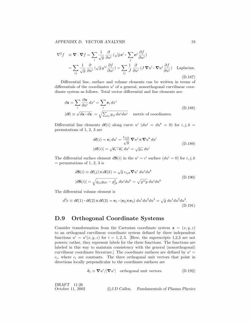
APPENDIX D. VECTOR ANALYSIS 19
∇2f ≡ ∇ · ∇f =∑
i
1√g
∂
∂ui(√
g ei ·∑
j
ej ∂f
∂uj)
=∑ij
1√g
∂
∂ui(√
g gij ∂f
∂uj) =
∑ij
1J
∂
∂ui(J ∇ui · ∇uj ∂f
∂uj) Laplacian.
(D.187)Differential line, surface and volume elements can be written in terms of
differentials of the coordinates ui of a general, nonorthogonal curvilinear coor-dinate system as follows. Total vector differential and line elements are:
dx =∑
i
∂x∂ui
dxi =∑
i
ei dxi
|d"| ≡ √dx · dx =
√∑ij gij duiduj metric of coordinates.
(D.188)
Differential line elements d"(i) along curve ui (duj = duk = 0) for i, j, k =permutations of 1, 2, 3 are
d"(i) = ei dui =εijk√
g∇uj×∇uk dui
|d"(i)| =√
ei · ei dui = √gii dui
(D.189)
The differential surface element dS(i) in the ui = ci surface (dui = 0) for i, j, k= permutations of 1, 2, 3 is
dS(i) ≡ d"(j)×d"(k) =√
g εijk∇ui dujduk
|dS(i)| =√
gjjgkk − g2jk dujduk =
√giig dujduk
(D.190)
The differential volume element is
d3x ≡ d"(1) · d"(2)×d"(3) = e1 · (e2×e3) du1du2du3 =√
g du1du2du3.(D.191)
D.9 Orthogonal Coordinate Systems
Consider transformation from the Cartesian coordinate system x = (x, y, z)to an orthogonal curvilinear coordinate system defined by three independentfunctions ui = ui(x, y, z) for i = 1, 2, 3. [Here, the superscripts 1,2,3 are notpowers; rather, they represent labels for the three functions. The functions arelabeled in this way to maintain consistency with the general (nonorthogonal)curvilinear coordinate literature.] The coordinate surfaces are defined by ui =ci, where ci are constants. The three orthogonal unit vectors that point indirections locally perpendicular to the coordinate surfaces are
ei ≡ ∇ui/|∇ui| orthogonal unit vectors. (D.192)
DRAFT 11:26October 11, 2002 c©J.D Callen, Fundamentals of Plasma Physics

APPENDIX D. VECTOR ANALYSIS 20
For the simplest orthogonal coordinate system, the Cartesian coordinate system,e1 = ∇x = x, e2 = ∇y = y, e3 = ∇z = z.
Because of the normalization and assumed orthogonality of these unit vec-tors,
ei · ej = δij ≡
1, for i = j,0, for i (= j,
Kronecker delta. (D.193)
The cross products of unit vectors are governed by the right-hand rule which isembodied in the mathematical relation
ei×ej = εijk ek (D.194)
in which the Levi-Civita symbol εijk is defined by
εijk ≡ +1, for i, j, k = 1, 2, 3 or 2, 3, 1 or 3, 1, 2 (even permutations)
−1, for i, j, k = 2, 1, 3 or 1, 3, 2 or 3, 2, 1 (odd permutations)0, for any two indices the same.
(D.195)A vector A can be represented in terms of its components in the orthogonal
directions (parallel to ∇ui) of the unit vectors ei:
A =∑
i
Aiei = A1e1 + A2e2 + A3e3, Ai ≡ A · ei (D.196)
For an orthogonal coordinate system the identity dyad or tensor is
I =∑
i
eiei = e1e1 + e2e2 + e3e3 identity tensor. (D.197)
Thus, the vector differential operator becomes
∇ = I · ∇ =∑
i
ei (ei · ∇) = e1 (e1 · ∇) + e2 (e2 · ∇) + e3 (e3 · ∇)
=∑
i
∇ui ∂
∂ui= ∇u1 ∂
∂u1+ ∇u2 ∂
∂u2+ ∇u3 ∂
∂u3.
(D.198)
Here and below the sum over i is over the three components 1,2,3.Using the relations for the dot and cross products of the unit vectors ei given
in (D.193) and (D.194) the dot, cross and dot-cross products of vectors become
A · B =∑
i
AiBi = A1B1 + A2B2 + A3B3, (D.199)
A×B =∑ij
AiBj ei×ej =∑ijk
εijk AiBj ek =
∥∥∥∥∥∥e1 e2 e3
A1 A2 A3
B1 B2 B3
∥∥∥∥∥∥= e1(A2B3 − A3B2) + e2(A3B1 − A1B2) + e3(A1B2 − A2B1). (D.200)
A · B×C =∑ijk
εijk AiBjCk =
∥∥∥∥∥∥A1 A2 A3
B1 B2 B3
C1 C2 C3
∥∥∥∥∥∥ . (D.201)
DRAFT 11:26October 11, 2002 c©J.D Callen, Fundamentals of Plasma Physics

APPENDIX D. VECTOR ANALYSIS 21
The differential line element in the ith direction is given by
d"(i) = ei hi dui, with hi ≡ 1/|∇ui|, differential line element. (D.202)
Thus, the differential surface vector for the ui = ci surface, which is defined bydS(i) = d"(j)×d"(k), becomes
dS(i) = ei hjhk dujduk, for i (= j (= k, differential surface area. (D.203)
Since the differential volume element is d3x = d"(i) · dS(i) = d"(1) · d"(2)×d"(3)and the Jacobian of the transformation is given by J = 1/(∇u1 · ∇u2×∇u3)= h1h2h3,
d3x = h1h2h3 du1du2du3, differential volume. (D.204)
For orthogonal coordinate systems the various partial derivatives in spaceare
∇f =∑
i
ei
hi
∂f
∂ui=
∑i
ei (ei · ∇) f, (D.205)
∇ · A =∑
i
1J
∂
∂ui
(J
hiA · ei
)=
∑i
1h1h2h3
∂
∂ui
(h1h2h3
hiA · ei
), (D.206)
∇×A =∑ijk
εijkhkek
J
∂
∂ui(hjA · ej) =
∑ijk
εijkhkek
h1h2h3
∂
∂ui(hjA · ej), (D.207)
∇2f =∑
i
1J
∂
∂ui
(J
h2i
∂f
∂ui
)=
∑i
1h1h2h3
∂
∂ui
(h1h2h3
h2i
∂f
∂ui
). (D.208)
The three most common orthogonal coordinate systems are the Cartesian,cylindrical, and spherical coordinate systems. Their coordinate surfaces andunit vectors are shown in Fig. D.3. They will be defined in this book by
Cartesian : ui = (x, y, z)hx = 1, hy = 1, hz = 1 =⇒ J = 1; (D.209)
cylindrical : ui = (r, θ, z)
r ≡√
x2 + y2, θ ≡ arctan(y/x), z ≡ z,
x = r cos θ, y = r sin θ, z = z,
hr = 1, hθ = r, hz = 1 =⇒ J = r; (D.210)
spherical : ui = (r,ϑ,ϕ)
r ≡√
x2 + y2 + z2, ϑ ≡ arctan(√
x2 + y2/r), ϕ ≡ arctan(y/x),x = r sinϑ cosϕ, y = r sinϑ sinϕ, z = r cosϑ,
hr = 1, hθ = r, hϕ = r sinϑ =⇒ J = r2 sinϑ. (D.211)
DRAFT 11:26October 11, 2002 c©J.D Callen, Fundamentals of Plasma Physics
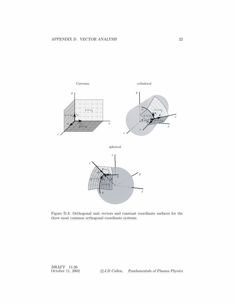
APPENDIX D. VECTOR ANALYSIS 22
x
y
z
r
ϕ
x!=!c1
y!=!c2
z!=!c3
r!=!c1ϕ!=!c2
z!=!c3
r!=!c1
ϕ!=!c3
x
x
y
z
x
y
z
x
r
ϕ
z
Cartesian cylindrical
spherical
!=!c
Figure D.3: Orthogonal unit vectors and constant coordinate surfaces for thethree most common orthogonal coordinate systems.
DRAFT 11:26October 11, 2002 c©J.D Callen, Fundamentals of Plasma Physics
APPENDIX D. VECTOR ANALYSIS 23
Note that with these definitions the cylindrical angle θ is the same as the az-imuthal (longitudinal) spherical angle ϕ, but that the radial coordinate r isdifferent in the cylindrical and spherical coordinate systems. The spherical an-gle ϑ is a latitude angle — see Fig. D.3. Explicit forms for the various partialderivatives in space, (D.205) – (D.208), are given in Appendix Z.
REFERENCES
Intermediate level discussions of vector analysis are provided in
Greenberg, Advanced Engineering Mathematics, Chapters 13-16 (1998) [?]
Kusse and Westwig, Mathematical Physics (1998) [?]
Danielson, Vectors and Tensors in Engineering and Physics, 2nd Ed. (1997) [?]
More advanced treatments are available in
Arfken, Mathematical Methods for Physicists (??) [?]
Greenberg, Foundations of Applied Mathematics, Chapters 8,9 (1978) [?]
Morse and Feshbach, Methods of Theoretical Physics, Part I, Chapter 1 (1953)[?]
DRAFT 11:26October 11, 2002 c©J.D Callen, Fundamentals of Plasma Physics

APPENDIX F. TRANSFORMS, COMPLEX ANALYSIS 1
Appendix F
Transforms, ComplexAnalysis
This appendix discusses Fourier and Laplace transforms as they are used inplasma physics and this book. Also, key properties of complex variable theorythat are needed for understanding and inverting these transforms, and to definesingular integrals that arise in plasma physics, are summarized here.
Fourier and Laplace transforms are useful in solving differential equations be-cause they convert differentiation in the dependent variable into multiplicationby the transform variable. Thus, they convert linear differential equations intoalgebraic equations in the transformed variables. In addition, Laplace trans-forms introduce the (temporal) initial conditions and hence causality into thetransformed equations and the ultimate (inverse transform) solution.
F.1 Fourier Transforms
Fourier transforms are usually used for representing spatial variations becausethe spatial domain of the response is often localized away from the boundaries.For such situations the spatial domain can be considered infinite: |x| ≤ ∞. TheFourier transform F (transformed functions are indicated by hats over them)and its inverse F−1 are defined in three dimensions by1
f(k) = Ff(x) ≡∫
d3x e−ik·xf(x), Fourier transform, (F.1)
f(x) ae= F−1f(k) ≡∫
d3k
(2π)3eik·xf(k), inverse Fourier transform. (F.2)
1The “ae” above the equal sign in the second equation is there to remind us that the inversetransform is equal to the original function “almost everywhere” — namely, everywhere thefunction f is continuous. At a jump discontinuity the inverse transform is equal to the averageof the function across the discontinuity: [f(x + 0) + f(x − 0)]/2.
DRAFT 12:20August 19, 2003 c©J.D Callen, Fundamentals of Plasma Physics
APPENDIX F. TRANSFORMS, COMPLEX ANALYSIS 2
These three dimensional integrals are defined in cartesian coordinates by∫d3x ≡
∫ ∞
−∞dx
∫ ∞
−∞dy
∫ ∞
−∞dz,
∫d3k ≡
∫ ∞
−∞dkx
∫ ∞
−∞dky
∫ ∞
−∞dkz. (F.3)
Sufficient conditions for the integral in the Fourier transform to converge are thatf(x) be piecewise smooth and that the integral of f(x) converges absolutely:∫
d3x |f(x)| < constant, Fourier transform convergence condition. (F.4)
When these conditions are satisfied, the inverse Fourier transform yields theoriginal function f(x) at all x except at a discontinuity in the function where ityields the average of the values of f(x) on the two sides of the discontinuity.
Some useful Fourier transforms are (here k2 ≡ k · k)
F1 = (2π)3 δ(k), (F.5a)
Fδ(x − x0) = e−ik·x0 , (F.5b)
Feik0·x = (2π)3 δ(k − k0), (F.5c)
Fe−|x|/∆/|x| = 4π/(k2 + 1/∆2), (F.5d)
Fe−|x|2/2∆2 = (√
2π∆)3 e−k2∆2/2, (F.5e)
Ff(x) = f(k), (F.5f)
F∇f(x) = ik f(k), (F.5g)
F∇ · A = ik · A(k), (F.5h)
F∇×A(x) = ik×A(k), (F.5i)
F∇2f(x) = − k2f(k), (F.5j)
F∫ d3x′ G(x − x′) f(x′) = G(k) f(k). (F.5k)
(F.5)
The last relation is called the Fourier convolution relation. Corresponding in-verse Fourier transforms can be inferred by taking the inverse Fourier transformsof these relations and using the fact that F−1Ff(x) ae= f(x).
As can be seen from (F.5e), which is indicative of the Fourier transformof the smoothest possible localized function in space, the localization in space(δxrms = ∆) times the localization in k-space (δkrms = 1/∆) is subject to thecondition:
δk δx ≥ 1, uncertainty relation.2 (F.6)Taking the dot product of the Fourier transform of a vector field with its
complex conjugate and integrating over all k-space yields∫d3x |A(x)|2 =
∫d3k
(2π)3|A(k)|2, Parseval’s theorem. (F.7)
2This uncertainty relation indicates the degree of localization in k-space for a given local-ization of a function in x-space. For the energy density in wave-packets and the probabilitydensity in quantum mechanics, the corresponding uncertainty principle is determined using thesquare of the fluctuating field or wave function; then the uncertainty principle is δk δx ≥ 1/2.
DRAFT 12:20August 19, 2003 c©J.D Callen, Fundamentals of Plasma Physics

APPENDIX F. TRANSFORMS, COMPLEX ANALYSIS 3
F.2 Laplace Transforms
Laplace transforms are often used to analyze the temporal evolution in responseto initial conditions from the present time (t = 0) forward in time, which definesan infinite half-space time domain (0 < t < ∞) problem. The Laplace transformL and its inverse L−1 are defined by3
f(ω) = Lf(t) ≡∫ ∞
0−dt eiωtf(t), Laplace transform, (F.8)
f(t) ae= L−1f(ω) ≡∫ ∞+iσ
−∞+iσ
dω
2πe−iωtf(ω), inverse Laplace transform. (F.9)
Sufficient conditions for the Laplace transform integral to converge are that f(t)be piecewise smooth and at most of exponential order:
limt→∞ f(t) < constant× eσt, Laplace transform convergence condition, (F.10)
which defines the convergence parameter σ needed for the path of integration inthe inverse Laplace transform (F.9). The function f(t) can grow exponentiallyin time like eγt; then σ > γ is required for (F.10) to be satisfied. The obtainedtransform f(ω) is only valid for Imω > σ. As indicated by the “ae” (almosteverywhere) over the equal sign in (F.9), the inverse Laplace transform yieldsthe original function f(t) for all t except at a discontinuity in the function whereit yields the average of the values of f(t) on the two sides of the discontinuity.Because the original function and its inverse Laplace transform are only valid fort ≥ 0, some people introduce a Heaviside step function H(t) (see Section B.1)into the integral in the definition of the inverse transform in (F.9) to emphasizethat fact.
3In plasma physics it is convenient to use eiωt as the integrating factor in the definitionof the Laplace transform so that when ω is real it will represent a (radian) frequency. Manymathematics texts use e−st or e−pt (iω ⇐⇒ −s or −p) as the integrating factor to emphasizeexponential growth or damping. Most electrical engineering texts use e−jωt (iω ⇐⇒ −jω).
DRAFT 12:20August 19, 2003 c©J.D Callen, Fundamentals of Plasma Physics

APPENDIX F. TRANSFORMS, COMPLEX ANALYSIS 4
Some useful Laplace transforms are
Le−νt =i
ω + iν, σ > −ν, (F.11a)
Le−iωt =i
ω − ω, σ > Imω, (F.11b)
Leγt sin(ω0t) =−ω0
(ω − iγ)2 − ω20
, σ > γ, (F.11c)
Leγt cos(ω0t) =i (ω − iγ)
(ω − iγ)2 − ω20
, σ > γ, (F.11d)
L
e−x2/4Dt
√πt
=
e−x√
−iω/D
√−iω, (F.11e)
LH(t) =i
ω=
1− iω
, (F.11f)
Lδ(t) = 1, (F.11g)
Ldδ(t)dt
= − iω, (F.11h)
L
e−iωt
√t
=
√π
−i(ω − ω), (F.11i)
Lf(t) = f(ω), (F.11j)
Lf(t) = − iωf(ω) − f(0), (F.11k)
Lf(t) = −ω2f(ω) + iωf(0) − f(0), (F.11l)
Ltnf(t) =1in
dnf(ω)dωn
, (F.11m)
L∫ t0 dt′ G(t − t′) f(t′) = G(ω) f(ω). (F.11n)
(F.11)In (F.11b) and (F.11i) the frequency ω is in general complex. In (F.11c) and(F.11d) the frequency ω0 and gowth rate γ are real. In (F.11g) and (F.11h)the integrals over the delta functions are evaluated by taking account of thelower limit of the Laplace transform integral being 0− (an infinitesimal negativetime near zero) where the delta function vanishes. The last relation is calledthe Laplace convolution relation. Corresponding inverse Laplace transformscan be inferred by taking the inverse Laplace transforms of these relations andusing the fact that L−1Lf(t) ae= f(t). [A Heaviside unit step function H(t)(see Section B.1) is sometimes inserted to remind one that Laplace transformsare only defined for t > 0, i.e., L−1Lf(t) ae= H(t)f(t).] The simultaneouslocalization in time and frequency is subject to a condition similar to (F.6):
δω δt ≥ 1, uncertainty relation. (F.12)
It is important to be aware of the differences between Fourier and Laplacetransforms. The main difference is that Fourier transforms represent functions
DRAFT 12:20August 19, 2003 c©J.D Callen, Fundamentals of Plasma Physics
APPENDIX F. TRANSFORMS, COMPLEX ANALYSIS 5
in infinite domains (in space) that have no starting or ending points and nopreferred directions of motion in them. In contrast, Laplace transforms rep-resent functions in an infinite half-space of time that begins (with suitable in-titial conditions) at t = 0, increases monotonically, and extends to an infinitetime in the future (t → ∞). These physical differences are manifested math-ematically in their transforms of unity. From (F.5a), the Fourier transform ofunity is F1 = (2π)3δ(k), which is a function of k that is singular at k = 0.In contrast, from (F.11a) with ν → 0, the corresponding Laplace transfom isL1 = i/ω, Imω > 0, which is singular for ω → 0 but with the nature ofthe singularity defined (see Sections F.4 to F.6) by the condition Imω > σ.Physically, this condition implies that as time progresses the response growsless rapidly than eσt. Thus, Laplace transforms embody the physical propertyof causality that the response proceeds sequentially in time from its initial condi-tions whereas Fourier transforms embody no such directionality in the response(or dependence on initial or boundary conditions). This key difference is oftenhighlighted by referring to the relevance of Laplace transforms for initial valueproblems and for ensuring temporal causality in the solution.
F.3 Combined Fourier-Laplace Transforms
Often we will need a combination of a three-dimensional Fourier transform inspace and a Laplace transform in time, which is defined by
f(k,ω) = FLf(x, t) ≡∫
d3x
∫ ∞
0−dt e−i(k·x−ωt) f(x, t). (F.13)
The corresponding combined inverse transform is defined by
f(x, t) ae= F−1L−1f(k,ω) ≡∫
d3k
(2π)3
∫ ∞+iσ
−∞+iσ
dω
2πei(k·x−ωt) f(k,ω). (F.14)
For a monochromatic wave [f(k,ω) = fk0,ω0(2π)4δ(k − k0)δ(ω − ω0)], we have
f(x, t) = fk0,ω0ei(k0·x−ω0t), three-dimensional plane wave. (F.15)
The representation of f(x, t) in terms of its transform f(k,ω) in (F.14) is avery useful form that is often used (for both scalar functions and vector fields)and one from which the Fourier and Laplace transforms of spatial and temporalderivatives in (F.5f)–(F.5j) and (F.11j)–(F.11l) can be deduced readily.
F.4 Properties of Complex Variables, Functions
A complex variable z = x + iy is a two-dimensional variable (vector) that hasreal [x ≡ Rez ≡ zR] and imaginary [y ≡ Imz ≡ zI ] parts. Its cartesian andpolar angle representations are
z = x + iy = zR + izI = reiθ, r ≡ |z| =√
z∗z =√
x2 + y2, θ = arctan y/x.(F.16)
DRAFT 12:20August 19, 2003 c©J.D Callen, Fundamentals of Plasma Physics
APPENDIX F. TRANSFORMS, COMPLEX ANALYSIS 6
The function eiθ is repesented by
eiθ = cos θ + i sin θ, Euler’s formula. (F.17)
Thus, the imaginary unit number i ≡ √−1 = eiπ/2. [More generally, one definesi = ei(4n+1)π/2, n = 0,±1,±2, . . ..] The complex conjugate of z is
z∗ = x − iy = |z|e−iθ, complex conjugate. (F.18)
The reciprocal of a complex variable can be written many ways:
1z
=1
x + iy=
x − iy
(x + iy)(x − iy)=
x − iy
x2 + y2=
z∗
|z|2 =e−iθ
|z| . (F.19)
A function of a complex variable w(z) ≡ wR(z)+i wI(z) is analytic at a pointz ≡ zR + i zI if its derivative dw/dz exists there and is the same irrespectiveof the direction in the complex z-plane along which the derivative is calculated.This criterion for a function to be analytic yields the sufficient conditions
∂wR
∂zR=
∂wI
∂zI,
∂wR
∂zI= −∂wI
∂zR, Cauchy-Riemann conditions for analyticity.
(F.20)A general expansion of a complex function around z = z0 is
w(z) =∞∑
n=−∞cn(z − z0)n, Laurent expansion. (F.21)
This expansion reduces to a Taylor series expansion if cn = 0 for all n < 0; then,cn = (1/n!) dnf/dzn|z=z0 , n = 0, 1, 2, . . ..
All functions that are analytic over a region can be expressed in terms ofconvergent Taylor series, with the radius of convergence bounded by the dis-tance from the expansion point to the nearest singularity. Examples of (entire)functions that are analytic over the entire finite z-plane are z, zn, sin z, ez. Onthe other hand, the function w1(z) = 1 + z + z2 + · · · has a radius of con-vergence |z| < 1. An analytic function can be analytically continued to ad-jacent regions where the function is analytic through Taylor series expansionabout other points in the original analytic region or by other means. For ex-ample, the power series in the function w1(z) above can be summed to yieldw1(z) = 1/(1 − z) = −1/(z − 1), which can be represented by a Laurent serieswith c−1 = −1 and z0 = 1 with all other cn = 0. The function −1/(z − 1) isanalytic everywhere except at z = 1 and represents the analytic continuation ofthe power series respresentation of w1(z) to all z += 1.
Nonanalytic functions have singularities (z values where they are unboundedor about which they are multivalued) and are represented by the Laurent serieswith cn += 0 for some n < 0. Isolated singularities are classified as follows:
• Poles. If the maximum negative power in the Laurent expansion (F.21)is m (i.e., c−m += 0 and c−n = 0 for n > m), then the function w(z) hasan mth-order pole at z = z0. For example, w1(z) = −1/(z − 1) has afirst-order pole at z = 1 and 1/(z − 1)2 has a second-order pole at z = 1.
DRAFT 12:20August 19, 2003 c©J.D Callen, Fundamentals of Plasma Physics
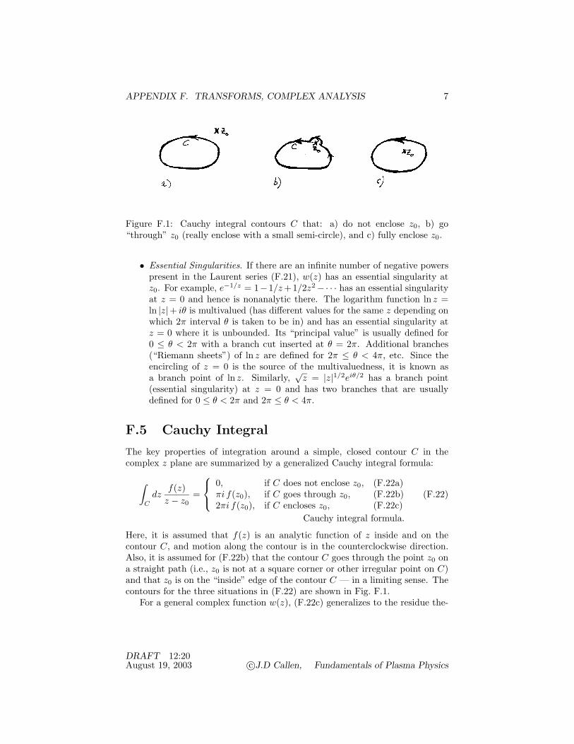
APPENDIX F. TRANSFORMS, COMPLEX ANALYSIS 7
Figure F.1: Cauchy integral contours C that: a) do not enclose z0, b) go“through” z0 (really enclose with a small semi-circle), and c) fully enclose z0.
• Essential Singularities. If there are an infinite number of negative powerspresent in the Laurent series (F.21), w(z) has an essential singularity atz0. For example, e−1/z = 1−1/z +1/2z2 − · · · has an essential singularityat z = 0 and hence is nonanalytic there. The logarithm function ln z =ln |z|+ iθ is multivalued (has different values for the same z depending onwhich 2π interval θ is taken to be in) and has an essential singularity atz = 0 where it is unbounded. Its “principal value” is usually defined for0 ≤ θ < 2π with a branch cut inserted at θ = 2π. Additional branches(“Riemann sheets”) of ln z are defined for 2π ≤ θ < 4π, etc. Since theencircling of z = 0 is the source of the multivaluedness, it is known asa branch point of ln z. Similarly,
√z = |z|1/2eiθ/2 has a branch point
(essential singularity) at z = 0 and has two branches that are usuallydefined for 0 ≤ θ < 2π and 2π ≤ θ < 4π.
F.5 Cauchy Integral
The key properties of integration around a simple, closed contour C in thecomplex z plane are summarized by a generalized Cauchy integral formula:
∫C
dzf(z)
z − z0=
0, if C does not enclose z0, (F.22a)πi f(z0), if C goes through z0, (F.22b)2πi f(z0), if C encloses z0, (F.22c)
(F.22)
Cauchy integral formula.
Here, it is assumed that f(z) is an analytic function of z inside and on thecontour C, and motion along the contour is in the counterclockwise direction.Also, it is assumed for (F.22b) that the contour C goes through the point z0 ona straight path (i.e., z0 is not at a square corner or other irregular point on C)and that z0 is on the “inside” edge of the contour C — in a limiting sense. Thecontours for the three situations in (F.22) are shown in Fig. F.1.
For a general complex function w(z), (F.22c) generalizes to the residue the-
DRAFT 12:20August 19, 2003 c©J.D Callen, Fundamentals of Plasma Physics
APPENDIX F. TRANSFORMS, COMPLEX ANALYSIS 8
orem for a contour C that encloses isolated pole-type singularities at z = zj :∫C
dz w(z) = 2πi∑
j
c−1(zj), Cauchy residue theorem. (F.23)
Here, c−1(zj) is the residue [coefficient c−1 in the Laurent expansion (F.21)] ofthe function w(z) at the singular point z = zj , which is defined by
c−1(zj) = limz→zj
[(z − zj)w(z)], first-order pole, (F.24a)
c−1(zj) =1
(m − 1)!lim
z→zj
dm−1
dzm−1[(z − zj)mw(z)], mth-order pole. (F.24b)
(F.24)
F.6 Inverse Laplace Transform Example
To illustrate the use of these complex variable integration formulas (and developsome inverse transform concepts that are important in plasma physics), considertheir use in evaluating the inverse Laplace transform of the weakly damped(ν << ω0) oscillator problem given in (??): x + νx + ω2
0x = f(x, t). Forsimplicity, assume the initial conditions are x(0) = x0, x(0) = 0 [θ0 = π/2 inthe initial conditions used to derive (??)] and that there is no forcing function f .Taking the Laplace transform of the homogeneous damped oscillator equationand solving for the transform of the response, one obtains
x(ω) = G(ω)S(ω) =x0(ν − iω)
−ω2 − iνω + ω20
, S(ω) ≡ x0. (F.25)
The temporal response x(t) is obtained from the inverse Laplace transform:
x(t) = L−1x(ω) =∫ ∞+iσ
−∞+iσ
dω
2πI(ω), (F.26)
I(ω) = − e−iωtx0(ν − iω)(ω − ων + iν/2)(ω + ων + iν/2)
. (F.27)
The integrand I(ω) has first-order poles at ω = ω±, with residues given by
c−1(ω±) = ± e−iω±t(ν − iω±)2ων
, ω± ≡ ±ων − iν/2, ων ≡√ω2
0 − ν2/4.
(F.28)Figure F.2a illustrates the inverse Laplace transform integration path (L) in
(F.26) for an arbitrary σ > 0. As indicated, it is just a line integral from −∞+iσto ∞ + iσ along a line that is parallel to the ωR ≡ Reω axis, but a distanceωI ≡ Imω = σ above it. While for this problem we could convert this lineintegral into a closed contour by adding the (vanishing, for t > 0) integral alongthe infinite semi-circle in the lower half ω-plane [Csc with |ω| → ∞ as shownin Fig. F.2a], we will use a more generally useful procedure. [The vanishing of
DRAFT 12:20August 19, 2003 c©J.D Callen, Fundamentals of Plasma Physics
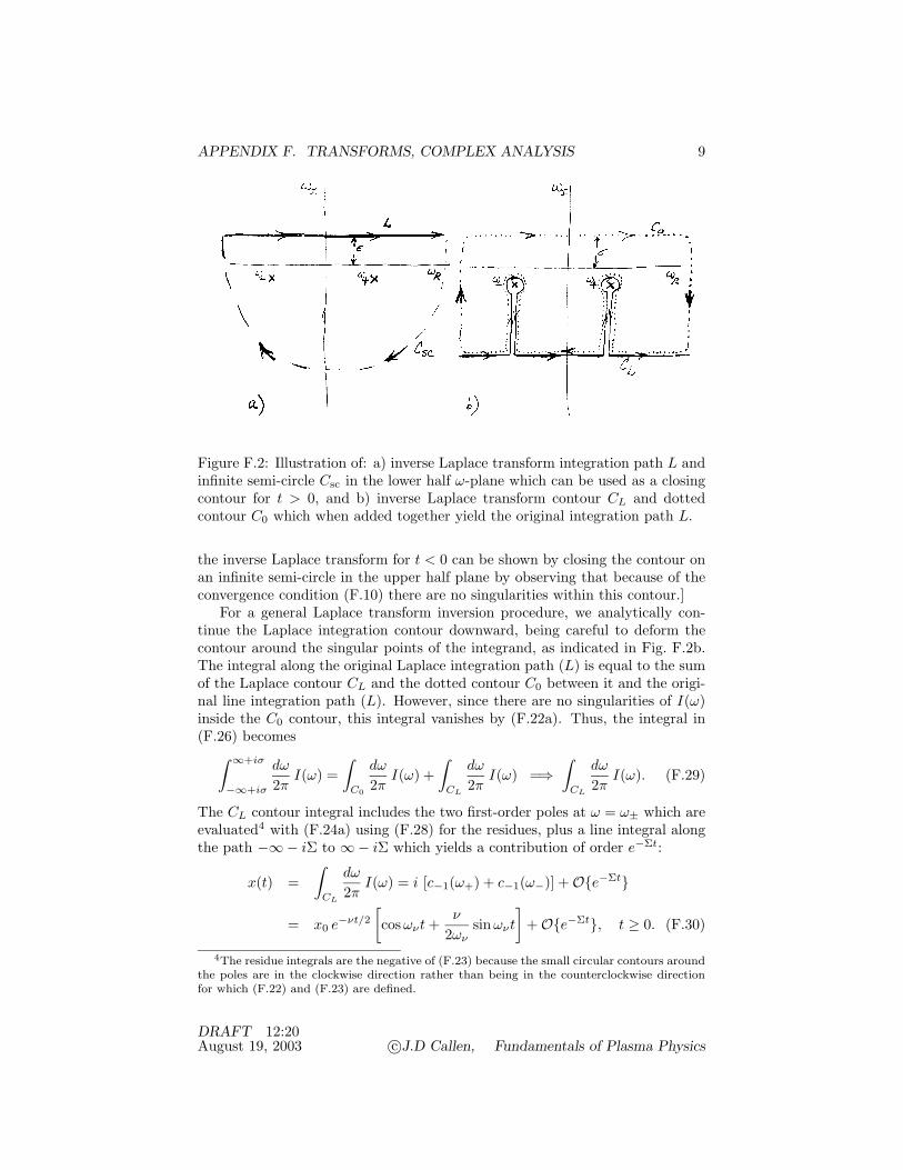
APPENDIX F. TRANSFORMS, COMPLEX ANALYSIS 9
Figure F.2: Illustration of: a) inverse Laplace transform integration path L andinfinite semi-circle Csc in the lower half ω-plane which can be used as a closingcontour for t > 0, and b) inverse Laplace transform contour CL and dottedcontour C0 which when added together yield the original integration path L.
the inverse Laplace transform for t < 0 can be shown by closing the contour onan infinite semi-circle in the upper half plane by observing that because of theconvergence condition (F.10) there are no singularities within this contour.]
For a general Laplace transform inversion procedure, we analytically con-tinue the Laplace integration contour downward, being careful to deform thecontour around the singular points of the integrand, as indicated in Fig. F.2b.The integral along the original Laplace integration path (L) is equal to the sumof the Laplace contour CL and the dotted contour C0 between it and the origi-nal line integration path (L). However, since there are no singularities of I(ω)inside the C0 contour, this integral vanishes by (F.22a). Thus, the integral in(F.26) becomes∫ ∞+iσ
−∞+iσ
dω
2πI(ω) =
∫C0
dω
2πI(ω) +
∫CL
dω
2πI(ω) =⇒
∫CL
dω
2πI(ω). (F.29)
The CL contour integral includes the two first-order poles at ω = ω± which areevaluated4 with (F.24a) using (F.28) for the residues, plus a line integral alongthe path −∞− iΣ to ∞− iΣ which yields a contribution of order e−Σt:
x(t) =∫
CL
dω
2πI(ω) = i [c−1(ω+) + c−1(ω−)] + Oe−Σt
= x0 e−νt/2
[cosωνt +
ν
2ωνsinωνt
]+ Oe−Σt, t ≥ 0. (F.30)
4The residue integrals are the negative of (F.23) because the small circular contours aroundthe poles are in the clockwise direction rather than being in the counterclockwise directionfor which (F.22) and (F.23) are defined.
DRAFT 12:20August 19, 2003 c©J.D Callen, Fundamentals of Plasma Physics
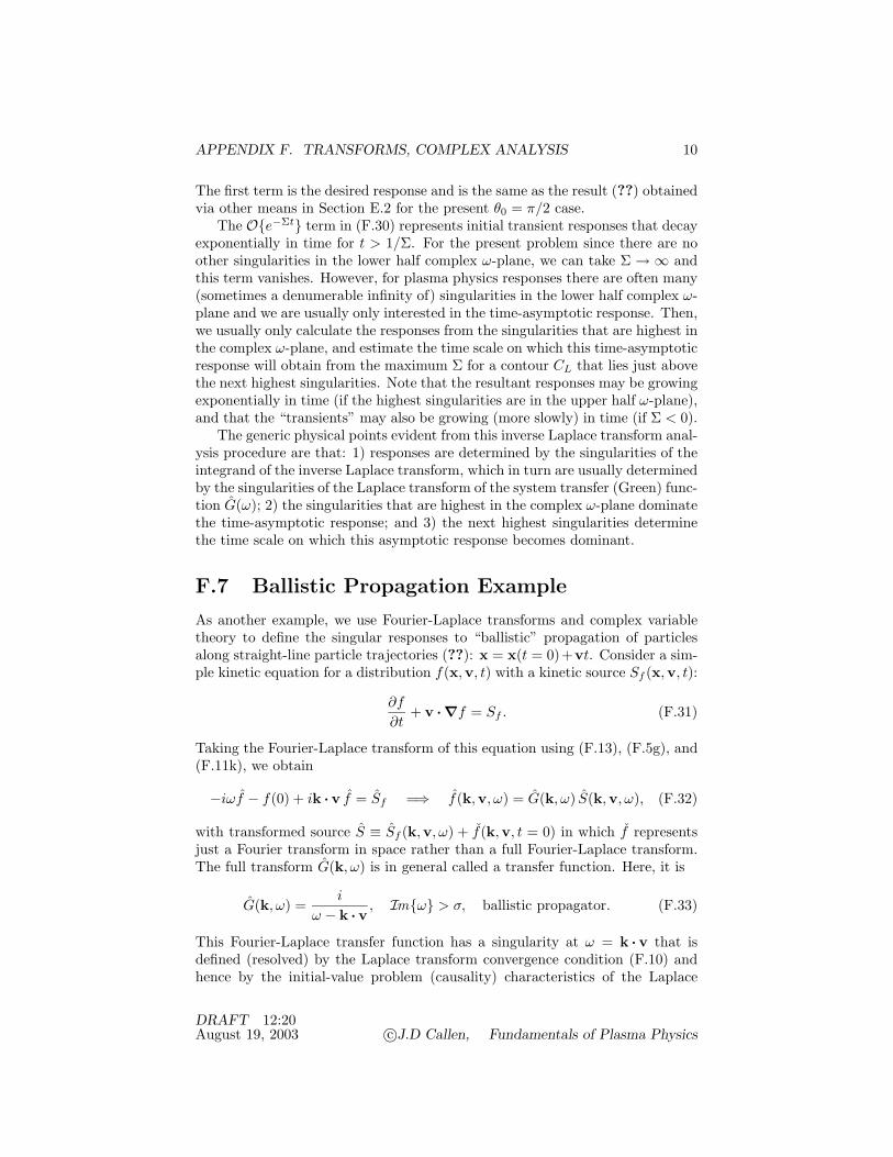
APPENDIX F. TRANSFORMS, COMPLEX ANALYSIS 10
The first term is the desired response and is the same as the result (??) obtainedvia other means in Section E.2 for the present θ0 = π/2 case.
The Oe−Σt term in (F.30) represents initial transient responses that decayexponentially in time for t > 1/Σ. For the present problem since there are noother singularities in the lower half complex ω-plane, we can take Σ → ∞ andthis term vanishes. However, for plasma physics responses there are often many(sometimes a denumerable infinity of) singularities in the lower half complex ω-plane and we are usually only interested in the time-asymptotic response. Then,we usually only calculate the responses from the singularities that are highest inthe complex ω-plane, and estimate the time scale on which this time-asymptoticresponse will obtain from the maximum Σ for a contour CL that lies just abovethe next highest singularities. Note that the resultant responses may be growingexponentially in time (if the highest singularities are in the upper half ω-plane),and that the “transients” may also be growing (more slowly) in time (if Σ < 0).
The generic physical points evident from this inverse Laplace transform anal-ysis procedure are that: 1) responses are determined by the singularities of theintegrand of the inverse Laplace transform, which in turn are usually determinedby the singularities of the Laplace transform of the system transfer (Green) func-tion G(ω); 2) the singularities that are highest in the complex ω-plane dominatethe time-asymptotic response; and 3) the next highest singularities determinethe time scale on which this asymptotic response becomes dominant.
F.7 Ballistic Propagation Example
As another example, we use Fourier-Laplace transforms and complex variabletheory to define the singular responses to “ballistic” propagation of particlesalong straight-line particle trajectories (??): x = x(t = 0)+vt. Consider a sim-ple kinetic equation for a distribution f(x,v, t) with a kinetic source Sf (x,v, t):
∂f
∂t+ v · ∇f = Sf . (F.31)
Taking the Fourier-Laplace transform of this equation using (F.13), (F.5g), and(F.11k), we obtain
−iωf − f(0) + ik · v f = Sf =⇒ f(k,v,ω) = G(k,ω) S(k,v,ω), (F.32)
with transformed source S ≡ Sf (k,v,ω) + f(k,v, t = 0) in which f representsjust a Fourier transform in space rather than a full Fourier-Laplace transform.The full transform G(k,ω) is in general called a transfer function. Here, it is
G(k,ω) =i
ω − k · v , Imω > σ, ballistic propagator. (F.33)
This Fourier-Laplace transfer function has a singularity at ω = k · v that isdefined (resolved) by the Laplace transform convergence condition (F.10) andhence by the initial-value problem (causality) characteristics of the Laplace
DRAFT 12:20August 19, 2003 c©J.D Callen, Fundamentals of Plasma Physics

APPENDIX F. TRANSFORMS, COMPLEX ANALYSIS 11
transform. It is called the ballistic propagator in plasma physics because itrepresents [in ω,k transform space — see (F.35) below] motion along straight-line particle trajectories.
The kinetic distribution f is obtained from the full inverse transform:
f(x,v, t) = F−1L−1f =∫
d3k
(2π)3
∫ ∞+iσ
−∞+iσ
dω
2πei(k·x−ωt) G(k,ω)S(k,v,ω)
=∫ t
0−dt′
∫d3x′ G(x − x′, t − t′) S(x′,v, t′), t ≥ 0, (F.34)
in which the second line follows from combining the convolution integrals (F.5k)and (F.11n) that result from the inverse Fourier and Laplace transforms of theproducts of the two transforms G(k,ω) and S(k,v,ω). The Green functionG(x, t) is obtained by first using the same inverse Laplace transform procedureof deforming the Laplace integration contour (see Fig. F.2) downward aroundthe singularity (in this case at ω = k · v) as was used in the preceding analysis ofthe damped oscillator. Then, taking account of the first-order pole, evaluatingthe residue via (F.24a), and using the delta function definition in (??) withx → x − vt to evaluate the inverse Fourier transform, we obtain
G(x, t) = F−1L−1
i
ω − k · v
=∫
d3k
(2π)3eik·(x−vt) = δ(x − vt),
Green function. (F.35)
The inverse Fourier-Laplace transform of S is obtained using (F.2), (F.9) andL−1 of (F.11g):
S(x,v, t) = Sf (x,v, t) + f(x,v, t = 0) δ(t). (F.36)
Substituting (F.35) and (F.36) into (F.34), we obtain for t ≥ 0
f(x,v, t) =∫ t
0−dt′
∫d3x′ δ[x − x′ − v(t − t′)]S(x′,v, t′)
= f(x − vt,v, t = 0) +∫ t
0−dt′ Sf [x − v(t − t′),v, t′], (F.37)
which is the “ballistic” response we have been seeking. The first term representspropagation of the initial distribution function along the ballistic straight-lineparticle trajectories x = x(t = 0) + vt, while the second represents the timeintegral of the effect of the propagation of the source function along the sametrajectories. Since the solutions propagate (move along) the ballistic motion ofthe particles, these are called ballistic solutions. Hence, the transform of theGreen function that caused this response, which is given in (F.33), is called theballistic propagator.
DRAFT 12:20August 19, 2003 c©J.D Callen, Fundamentals of Plasma Physics
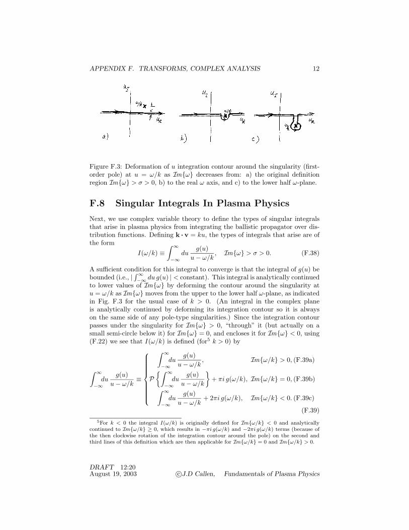
APPENDIX F. TRANSFORMS, COMPLEX ANALYSIS 12
Figure F.3: Deformation of u integration contour around the singularity (first-order pole) at u = ω/k as Imω decreases from: a) the original definitionregion Imω > σ > 0, b) to the real ω axis, and c) to the lower half ω-plane.
F.8 Singular Integrals In Plasma Physics
Next, we use complex variable theory to define the types of singular integralsthat arise in plasma physics from integrating the ballistic propagator over dis-tribution functions. Defining k · v = ku, the types of integrals that arise are ofthe form
I(ω/k) ≡∫ ∞
−∞du
g(u)u − ω/k
, Imω > σ > 0. (F.38)
A sufficient condition for this integral to converge is that the integral of g(u) bebounded (i.e., | ∫ ∞
−∞ du g(u) | < constant). This integral is analytically continuedto lower values of Imω by deforming the contour around the singularity atu = ω/k as Imω moves from the upper to the lower half ω-plane, as indicatedin Fig. F.3 for the usual case of k > 0. (An integral in the complex planeis analytically continued by deforming its integration contour so it is alwayson the same side of any pole-type singularities.) Since the integration contourpasses under the singularity for Imω > 0, “through” it (but actually on asmall semi-circle below it) for Imω = 0, and encloses it for Imω < 0, using(F.22) we see that I(ω/k) is defined (for5 k > 0) by
∫ ∞
−∞du
g(u)u − ω/k
≡
∫ ∞
−∞du
g(u)u − ω/k
, Imω/k > 0, (F.39a)
P∫ ∞
−∞du
g(u)u − ω/k
+ πi g(ω/k), Imω/k = 0, (F.39b)∫ ∞
−∞du
g(u)u − ω/k
+ 2πi g(ω/k), Imω/k < 0. (F.39c)
(F.39)5For k < 0 the integral I(ω/k) is originally defined for Imω/k < 0 and analytically
continued to Imω/k ≥ 0, which results in −πi g(ω/k) and −2πi g(ω/k) terms (because ofthe then clockwise rotation of the integration contour around the pole) on the second andthird lines of this definition which are then applicable for Imω/k = 0 and Imω/k > 0.
DRAFT 12:20August 19, 2003 c©J.D Callen, Fundamentals of Plasma Physics
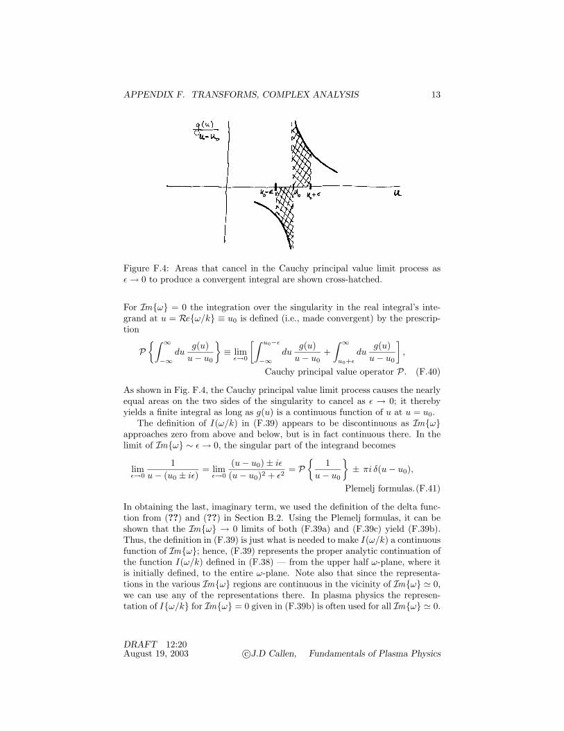
APPENDIX F. TRANSFORMS, COMPLEX ANALYSIS 13
Figure F.4: Areas that cancel in the Cauchy principal value limit process asε → 0 to produce a convergent integral are shown cross-hatched.
For Imω = 0 the integration over the singularity in the real integral’s inte-grand at u = Reω/k ≡ u0 is defined (i.e., made convergent) by the prescrip-tion
P∫ ∞
−∞du
g(u)u − u0
≡ lim
ε→0
[∫ u0−ε
−∞du
g(u)u − u0
+∫ ∞
u0+εdu
g(u)u − u0
],
Cauchy principal value operator P. (F.40)
As shown in Fig. F.4, the Cauchy principal value limit process causes the nearlyequal areas on the two sides of the singularity to cancel as ε → 0; it therebyyields a finite integral as long as g(u) is a continuous function of u at u = u0.
The definition of I(ω/k) in (F.39) appears to be discontinuous as Imωapproaches zero from above and below, but is in fact continuous there. In thelimit of Imω ∼ ε → 0, the singular part of the integrand becomes
limε→0
1u − (u0 ± iε)
= limε→0
(u − u0) ± iε
(u − u0)2 + ε2= P
1
u − u0
± πi δ(u − u0),
Plemelj formulas.(F.41)
In obtaining the last, imaginary term, we used the definition of the delta func-tion from (??) and (??) in Section B.2. Using the Plemelj formulas, it can beshown that the Imω → 0 limits of both (F.39a) and (F.39c) yield (F.39b).Thus, the definition in (F.39) is just what is needed to make I(ω/k) a continuousfunction of Imω; hence, (F.39) represents the proper analytic continuation ofthe function I(ω/k) defined in (F.38) — from the upper half ω-plane, where itis initially defined, to the entire ω-plane. Note also that since the representa-tions in the various Imω regions are continuous in the vicinity of Imω . 0,we can use any of the representations there. In plasma physics the represen-tation of Iω/k for Imω = 0 given in (F.39b) is often used for all Imω . 0.
DRAFT 12:20August 19, 2003 c©J.D Callen, Fundamentals of Plasma Physics

APPENDIX F. TRANSFORMS, COMPLEX ANALYSIS 14
REFERENCESDiscussions of transforms and complex variable theory are provided in most ad-
vanced engineering mathematics and mathematical physics textbooks, for example:
Greenberg, Advanced Engineering Mathematics (1988,1998), Chapts. 5, 21–24[?]
Greenberg, Foundations of Applied Mathematics (1978), Chapts. 6, 11–16 [?]
Morse and Feshbach, Methods of Theoretical Physics (1953), Vol. I, Chapt. 4[?]
Arfken, Mathematical Methods for Physicists (1970) [?]
Kusse and Westwig, Mathematical Physics (1998), Chapts. 6–9 [?]
Classic treatises on the theory of complex variables are
Whittaker and Watson, A Course of Modern Analysis (1902,1963) [?]
Copson, Theory of Functions of a Complex Variable (1935) [?]
Carrier, Crook, Pearson, Functions of a Complex Variable (1966) [?]
An extensive table of Fourier and Laplace (and other) transforms is provided in
Erdelyi, Tables of Integral Transforms, Vol. 1 (1954) [?]
DRAFT 12:20August 19, 2003 c©J.D Callen, Fundamentals of Plasma Physics
APPENDIX Z. USEFUL FORMULAS 1
Appendix Z
Useful Formulas
DRAFT 11:19February 2, 2002 c©J.D Callen, Fundamentals of Plasma Physics

APPENDIX Z. USEFUL FORMULAS 2
Key Vector Relations
A · B = B · A, A×B = − B×A, A×A = 0,
A · (B×C) = (A×B) · CA×(B×C) = B (A · C) − C (A · B), bac-cab rule
(A×B) · (C×D) = (A · C) (B · D) − (A · D) (B · C)
(A×B)×(C×D) = C (A×B · D) − D (A×B · C)
A = A‖b + A⊥ with b ≡ B/B
A‖ ≡ B · A/B = b · AA⊥ ≡ −B×(B×A)/B2 = − b×(b×A)
∇ · A = (B · ∇) (A‖/B) + (A‖/B) (∇ · B) + ∇ · A⊥
∇ · A⊥ = −A⊥· [∇ lnB + (b · ∇)b ] − (1/B) b · ∇×(B×A⊥)
For A⊥ = B×∇f/B2, b · ∇×(B×A⊥) = (b · ∇f) (b · ∇×b)
∇(fg) = g∇f + f∇g ∇ · ∇f ≡ ∇2f
∇ · (fA) = ∇f · A + f∇ · A ∇×∇f = 0
∇×(fA) = ∇f×A + f∇×A ∇ · ∇A ≡ ∇2A
∇ · (fT) = ∇f · T + f∇ · T = ∇ (∇ · A) − ∇×(∇×A)
∇×(fT) = ∇f×T + f∇×T ∇ · ∇×A = 0
(B · ∇)(A · C) = C · (B · ∇)A + A · (B · ∇)C
∇(A · B) = A×(∇×B) + B×(∇×A) + (A · ∇)B + (B · ∇)A
∇ · (AB) = B (∇ · A) + (A · ∇)B
∇ · (A×B) = B · ∇×A − A · ∇×B
∇×(A×B) = A (∇ · B) − B (∇ · A) + (B · ∇)A − (A · ∇)B
For the general coordinate x ≡ xex + yey + zez and |x| ≡ √x2 + y2 + z2,
∇ · x = 3, ∇×x = 0, ∇x = I, ∇ · I = 0, ∇× I = 0, A · I = A,
∇|x| = x/|x|, ∇(1/|x|) = −x/|x|3, ∇2(1/|x|) = − 4πδ(x), I · A = A.
For a volume V enclosed by a closed, continuous surface S,∫V d3x ∇ · A =
∫©∫
S dS · A, divergence, Gauss’ theorem.
For an open surface S bounded by a closed, continuous contour C,∫∫S dS · ∇×A =
∮C d! · A, Stokes’ theorem.
DRAFT 11:19February 2, 2002 c©J.D Callen, Fundamentals of Plasma Physics

APPENDIX Z. USEFUL FORMULAS 3
Explicit Forms Of Vector Differentiation Operators(ei ≡ ∇ui/|∇ui|, Ai ≡ ei · A)
Cartesian coordinates: ui = (x, y, z),∫
d3x =∫ ∞−∞ dx
∫ ∞−∞ dy
∫ ∞−∞ dz,
∇f = ex∂f
∂x+ ey
∂f
∂y+ ez
∂f
∂z
∇ · A =∂Ax
∂x+∂Ay
∂y+∂Az
∂z
∇×A = ex
[∂Az
∂y− ∂Ay
∂z
]+ ey
[∂Ax
∂z− ∂Az
∂x
]+ ez
[∂Ay
∂x− ∂Ax
∂y
]∇2f =
∂2f
∂x2+∂2f
∂y2+∂2f
∂z2
Cylindrical coordinates: ui = (r, θ, z),∫
d3x =∫ ∞0 r dr
∫ 2π0 dθ
∫ ∞−∞ dz,
with r ≡ √x2 + y2, θ ≡ arctan (y/x), z ≡ z,
and inverse relations x = r sin θ, y = r cos θ, z = z,
∇f = er∂f
∂r+ eθ
1r
∂f
∂θ+ ez
∂f
∂z
∇ · A =1r
∂
∂r(rAr) +
1r
∂Aθ
∂θ+∂Az
∂z
∇×A = er
[1r
∂Az
∂θ− ∂Aθ
∂z
]+ eθ
[∂Ar
∂z− ∂Az
∂r
]+ez
1r
[∂
∂r(rAθ) − ∂Ar
∂θ
]∇2f =
1r
∂
∂r
(r∂f
∂r
)+
1r2
∂2f
∂θ2+∂2f
∂z2
Spherical coordinates: ui = (r,ϑ,ϕ),∫
d3x =∫ ∞0 r2 dr
∫ π0 dϑ sinϑ
∫ 2π0 dϕ,
with r ≡ √x2 + y2 + z2, ϑ ≡ arctan (
√x2 + y2/r), ϕ ≡ arctan (y/x),
and inverse relations x = r sinϑ cosϕ, y = r sinϑ sinϕ, z = r cosϑ,
∇f = er∂f
∂r+ eϑ
1r
∂f
∂ϑ+ eϕ
1r sinϑ
∂f
∂ϕ
∇ · A =1r2
∂
∂r(r2Ar) +
1r sinϑ
∂
∂ϑ(sinϑAϑ) +
1r sinϑ
∂Aϕ
∂ϕ
∇×A = er1
r sinϑ
[∂
∂ϑ(sinϑAϕ) − ∂Aϑ
∂ϕ
]+eϑ
[1
r sinϑ∂Ar
∂ϕ− 1
r
∂
∂r(rAϕ)
]+ eϕ
1r
[∂
∂r(rAϑ) − ∂Ar
∂ϑ
]∇2f =
1r2
∂
∂r
(r2 ∂f
∂r
)+
1r2 sinϑ
∂
∂ϑ
(sinϑ
∂f
∂ϑ
)+
1r2 sin2 ϑ
∂2f
∂ϕ2
DRAFT 11:19February 2, 2002 c©J.D Callen, Fundamentals of Plasma Physics

APPENDIX Z. USEFUL FORMULAS 4
Physical Constants
me electron mass 9.11 × 10⁻³¹ kg, 511 keVmp proton mass 1.67 × 10⁻²⁷ kg, 938 MeVmp/me mass ratio 1836 = (42.85)2e elementary charge 1.602 × 10⁻¹⁹ C (= J/eV)c speed of light in vacuum 3 × 10⁸ m/s = 1/
√µ0ε0
µ0 permeability of vacuum 4π × 10−7 N/A2
ε0 permittivity of vacuum 8.85 × 10⁻¹² F/m, 4πε0 ' 10−10
h Planck constant 6.626 × 10⁻³⁴ J· sNA Avogadro constant 6.022 × 10²³#/mole/kB Boltzmann constant 11 600 K/eV
Key Plasma Formulas
Quantities are in SI (mks) units except temperature and energy which are ex-pressed in eV; Zi is the ion charge state; Ai ≡ mi/mp is the atomic mass number.
Frequencies
electron plasma ωpe ≡√
nee2
meε0 ' 56√
ne rad/s, fpe ' 9√
ne Hz
ion gyrofrequency ωci ≡ qi B
mi' 0.96 × 10⁸ Zi B
Airad/s
electron collision νe ≡ 43√πν(vTe) ' 5 × 10⁻¹¹ ne Zi
[Te(eV)]3/2
(lnΛ17
)s−1
Lengths
electron Debye λDe ≡√ε0Te
nee2' 7.4 × 10³
√Te(eV)
nem
ion gyroradius +i ≡ vTi
ωci' 1.4 × 10⁻⁴
√Ti(eV) Ai
ZiBm
electron collision λe =vTe
νe' 1.2 × 10¹⁶ [Te(eV)]2
ne Zi
(17
lnΛ
)m
Speeds, Velocities
electron thermal vTe ≡ √2 Te/me ' 5.9 × 10⁵
√Te(eV) m/s
ion thermal vTi ≡ √2 Ti/mi ' 1.4 × 10⁴
√Ti(eV)/Ai m/s
ion acoustic (Te >> Ti) cS ≡ √Zi Te/mi ' 104
√Zi Te(eV)/Ai m/s
Alfven cA ≡ B/√
µ0 ρm ' 2.2 × 10¹⁶B/√
ni Ai m/selectron diamagneticflow (dTe/dx = 0) V∗e ≡ Te
qeB
(1ne
dne
dx
)ey =
Te(eV)B Ln
ey m/s
electron drift in B(x)(average, low β) vDe =
2Te
qeB
(1B
dB
dx
)ey = − 2 Te(eV)
B LBey m/s
DRAFT 11:19February 2, 2002 c©J.D Callen, Fundamentals of Plasma Physics

APPENDIX Z. USEFUL FORMULAS 5
Drift, flow velocities (for +∇⊥ << 1, ω << ωc) perpendicular to B :
particle drift velocities plasma species flow velocities
vF = F×B/qB2 general force VF = F×B/qB2
vE = E×B/B2 E×B VE = E×B/B2
vµ = B×µ∇B/qB2 µ grad-Bµ ≡ mv2
⊥/2B
vκ = B×mv2‖κ/qB2 curvature
κ ≡ (b · ∇)b = −RC/R2C
diamagnetic V∗ = B×∇p/nqB2
vp = B×m(dvD/dt)/qB2 polarization Vp = B×m(dV/dt)/qB2
friction Vη = R×B/nqB2
viscosity Vπ = B×∇· π/nqB2
vD⊥ = vE + vµ + vκ total V = VE + V∗ + Vp + Vη + Vπ
Diffusivities
no magnetic field νeλ2e ≡ v2
Te/νe ' 7 × 10²¹ [Te(eV)]ne Zi
5/2( 17lnΛ
)m2/s
magnetic field η/µ0 ≡ (meνe/nee2)/µ0
' 1.4 × 10³
(Zi
[Te(eV)]3/2
) (lnΛ17
)m2/s
classical νe+2e = βe (η/µ0)
' 5.6 × 10⁻²² ne Zi
B2 [Te(eV)]1/2
(lnΛ17
)m2/s
Dimensionless
number of electronsin Debye cube ne λ3
De ' 4.1 × 10¹¹ [Te(eV)]3/2/√
ne
Coulomb logarithm lnΛ ≡ ln(
λD
max [ bclmin, bqm
min ]
)bclmin = Zi/(12πneλ2
De) ' 5 × 10⁻¹⁰Zi/Te(eV) m
bqmmin = h/(4πmev) ' 1.1 × 10⁻¹⁰/[Te(eV)]1/2 m
plasma tomagnetic pressure β ≡ ne Te + ni Ti
B2/2µ0
' 4.0 × 10⁻²⁵( ne
B2
)[Te(eV) +
ni
neTi(eV)
]Lundquist number S ≡ a2/(η/µ0)
L‖/cA
' 1.6 × 10¹³ a2B [Te(eV)]3/2
L‖ Zi√
ni Ai
(17
lnΛ
)
DRAFT 11:19February 2, 2002 c©J.D Callen, Fundamentals of Plasma Physics
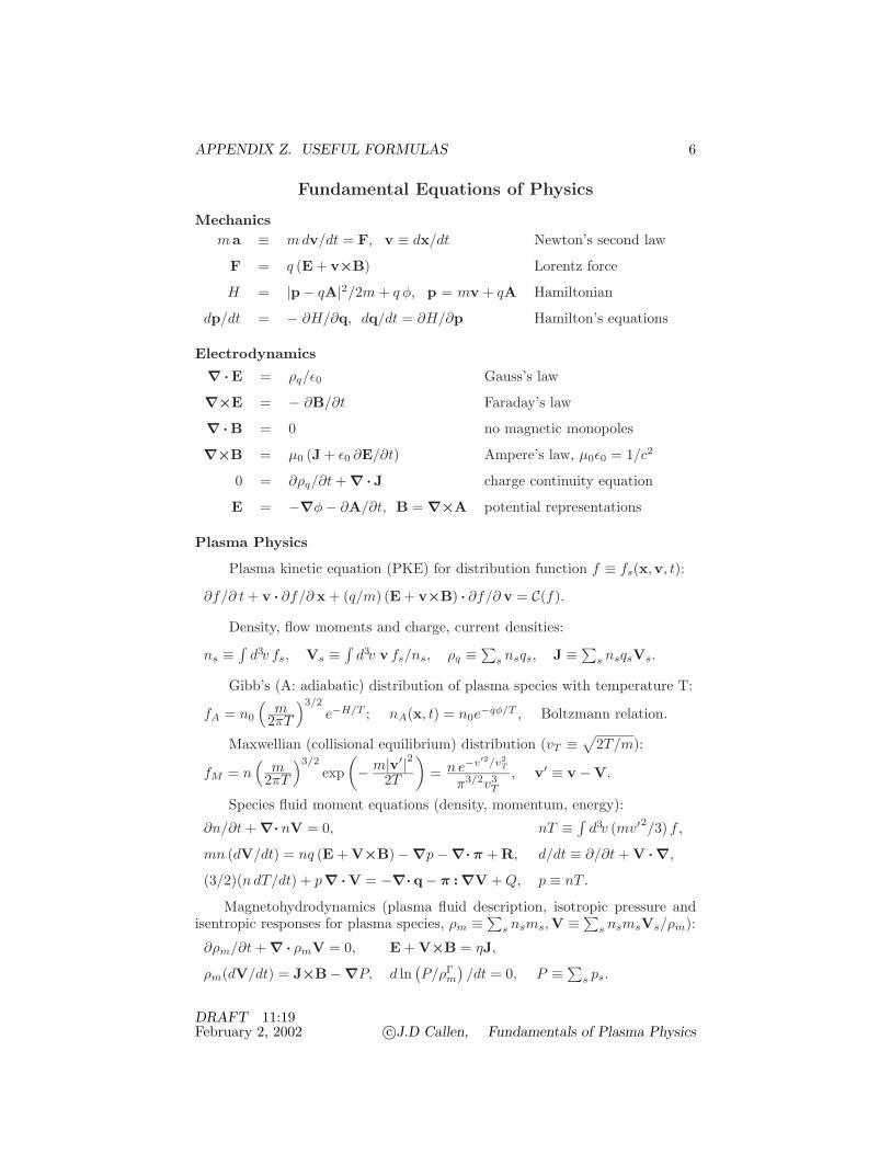
APPENDIX Z. USEFUL FORMULAS 6
Fundamental Equations of Physics
Mechanicsma ≡ m dv/dt = F, v ≡ dx/dt Newton’s second law
F = q (E + v×B) Lorentz force
H = |p − qA|2/2m + q φ, p = mv + qA Hamiltonian
dp/dt = − ∂H/∂q, dq/dt = ∂H/∂p Hamilton’s equations
Electrodynamics∇ · E = ρq/ε0 Gauss’s law
∇×E = − ∂B/∂t Faraday’s law
∇ · B = 0 no magnetic monopoles
∇×B = µ0 (J + ε0 ∂E/∂t) Ampere’s law, µ0ε0 = 1/c2
0 = ∂ρq/∂t + ∇ · J charge continuity equation
E = −∇φ− ∂A/∂t, B = ∇×A potential representations
Plasma Physics
Plasma kinetic equation (PKE) for distribution function f ≡ fs(x,v, t):
∂f/∂ t + v · ∂f/∂ x + (q/m) (E + v×B) · ∂f/∂ v = C(f).
Density, flow moments and charge, current densities:
ns ≡ ∫d3v fs, Vs ≡ ∫
d3v v fs/ns, ρq ≡ ∑s nsqs, J ≡ ∑
s nsqsVs.
Gibb’s (A: adiabatic) distribution of plasma species with temperature T:
fA = n0
(m
2πT
)3/2e−H/T ; nA(x, t) = n0e−qφ/T , Boltzmann relation.
Maxwellian (collisional equilibrium) distribution (vT ≡ √2T/m):
fM = n(
m2πT
)3/2exp
(− m|v′|2
2T
)= n e−v′2/v2
T
π3/2v3T
, v′ ≡ v − V.
Species fluid moment equations (density, momentum, energy):
∂n/∂t + ∇· nV = 0, nT ≡ ∫d3v (mv′2/3) f ,
mn (dV/dt) = nq (E + V×B) − ∇p − ∇· π + R, d/dt ≡ ∂/∂t + V · ∇,
(3/2)(n dT/dt) + p ∇ · V = −∇· q − π : ∇V + Q, p ≡ nT .
Magnetohydrodynamics (plasma fluid description, isotropic pressure andisentropic responses for plasma species, ρm ≡ ∑
s nsms,V ≡ ∑s nsmsVs/ρm):
∂ρm/∂t + ∇ · ρmV = 0, E + V×B = ηJ,
ρm(dV/dt) = J×B − ∇P, d ln(P/ρΓ
m
)/dt = 0, P ≡ ∑
s ps.
DRAFT 11:19February 2, 2002 c©J.D Callen, Fundamentals of Plasma Physics