í/f^ ¿dl^ ^'^^koa factor demand in

/í/f^ ¿dl^ United States ^'^^kOA uniiea oíaia»

lá^jl) Department of '^^^¡ Agriculture

Economic Research Service

Technical Bulletin Number 1765

Factor Demand in Imgated Agriculture Under Conditions of Restricted Water Supplies Daniel J. Bernardo Norman K. Whittlesey

Ni

Want Another Copy? It's Easy.

Just dial 1-800-999-6779. Toll free.

Ask for Factor Demand in Irrigated Agriculture Under Conditions of Restricted Water Supplies (TB-1765).

The cost is $5.50 per copy. For non-U.S. addresses, add 25 percent (includes Canada). Charge your purchase to your VISA or MasterCard, or we can bill you. Or send a check or purchase order (made payable to ERS-NASS) to:

ERS-NASS P.O. Box 1608 Rockville, MD 20850.

We'll fill your order by first-class mail.

FACTOR DEMAND IN IRRIGATED AGRICULTURE UNDER CONDITIONS OF RESTRICTED WATER SUPPLIES, by Daniel J. Bernardo and Norman K. Whittlesey. Resources and Technology Division, Economic Research Service, U.S. Department of Agriculture. Technical Bulletin No. 1765.

ABSTRACT

Irrigators can manage reduced water supplies by increasing the efficiency of water use through other inputs such as labor rather than removing land from production. The effect of reduced water supply on labor demand depends on the type of irrigation system used. Center pivot Irrigators' adoption of high-frequency schedules demands significantly more labor as water deficits are imposed. Sur- face Irrigators see a decrease in labor required as water supplies are initially reduced, but further water supply reductions result in increased labor demand. The potential for conserving water without greatly affecting producer returns runs up to 35 percent of irrigation water under surface irrigation and up to 25 percent under center pivot irrigation. This study uses a whole-farm irrigation management model to look at several limited water supply scenarios.

Keywords: center pivot irrigation, surface irrigation, irrigation, water restrictions

1301 New York Avenue, NW. Washington, DC 20005-4788 July 1989

ill

Contents

Introduction 1

Theoretical Constructs 1

The Empirical Model 3 Crop Simulation Model 3 Linkage of the Simulation and Optimization Stages 5 Mathematical Programming Model 5

Results 7 Surface Irrigation 8 Center Pivot Irrigation 10 Maximum Flow Rates 12

Conclusions 12

References 13

Factor Demand in Irrigated Agriculture Under Conditions of Restricted Water Supplies Daniel J. Bernardo* Norman K. Whittlesey

Introduction

Irrigated agriculture competes increasingly for available water supplies with municipal and industrial users throughout the Western United States. Some of these water users value water more highly in economic terms than does agriculture, but cannot acquire the necessary quantities due to agriculture's legal rights to water use. Institutional and legal changes are underway in many areas to meet society's goals by allocating water in a more economically efficient way among competing uses. Crop irrigation, as the largest user of water in the region, must meet this increasing competition for available water supplies by using them efficiently.

One region of particularly acute competition for available water supplies between irrigated agriculture and other users is the Pacific Northwest.

Irrigated agriculture in the region expanded rapidly in the last three decades, particularly in areas using water diverted from the Columbia River system. Over 8.3 million acres are currently irrigated in Idaho, Washington, and Oregon, with annual surface water withdrawals for irrigation exceeding 20.7 million acre-feet (6).^

These diversions significantly affect the region's hydroelectric generation, as well as instream water users. Principal irrigated crops in the region include wheat, barley, potatoes, sugar beets, field corn, sweet corn, orchard crops, and alfalfa, and account for over 65 percent of the region's direct farm income.

*The authors are assistant professor of agricultural economics, Oklahoma State University, and professor of agricultural economics, Washington State University. ERS supported work on this project through Cooperative Agreement No. 58-319V-6-00077 with Washington State University. This study also Is a contribution to Western Regional Project W-178.

^ Italicized numbers In parentheses refer to Items In the References.

Policymakers have proposed several institutional reforms for reallocating water supplies. Most proposed policies are either regulatory or market solutions. Proponents of regulatory reforms advocate regulations to enforce water conservation. Market solutions center on modifying institutional structure by creating water markets, and rely on private incentives to allocate water more efficiently. Whether reallocating water is mandated or voluntary, most reforms will eventually result in less water to agricultural producers.

Several researchers have recently addressed some of the issues involved in deriving efficient irrigation management plans with restricted water supplies. Re- search on allocating water supplies at the farm level uses a variety of research methods, including linear and dynamic programming, simulation, and multistage models. Most of these studies look at allocating scarce water supplies over time and space, ignoring the effect of water supply limits on other production factors. A question of considerable policy consequence concerns how land, labor, energy, and fertilizer use will change when water is scarce.

This report analyzes how restrictions on farm-level water supplies will affect the demand for irrigation and nonirrigation production factors, and draws inferences about options available to irrigators in the Pacific Northwest. This analysis requires a complete account- ing of all managerial and factor substitutions for dealing with limited water supplies. This study integrates knowledge regarding yield response to irrigation scheduling, application, and economics into a whole- farm irrigation management model. We apply the model to several limited water supply scenarios under conditions of irrigation.

Theoretical Constructs

We found that reducing water applied while minimizing reductions in crop uses requires changing the practices used to apply water. These changes may be both in

the timing and kind of irrigation and in the kind of nonirrigation inputs, such as nutrients, required.

Irrigation researchers disagree about the relationship between land use and optimal irrigation depth when water supply is limited. Hillel comments:

Traditionally, the great fallacy in water management has been the tendency to save water per unit of land area, in order to "green up" more land.... The best chance of increasing production efficiency by water management is to obviate water stress and prevent water from becoming a limiting factor of plant growth (7).

Conversely, some researchers support Stewart and others that "profit is maximized at some irrigation level below that associated with maximum yield" ( 12).

Much of this controversy stems from alternative assumptions on yield response to water deficits and the relative prices of irrigation inputs and output prices. The significance of these factors in deriving the optimal land-irrigation depth combination can be illustrated using the following example. We calculate returns per unit area as the product of yield per unit area (Y) and product price (P). Thus, over the irrigated area, returns (R) are expressed as:

or in practice

P . Y > r. Y + Ki + K2 • L(w) (5)

R = P • Y(w). A

where A is the number of acres irrigated.

(1)

Costs per unit area are calculated as the sum of yield- dependent cost, some constant per-unit-area cost, and water-dependent costs. Therefore, we express total net returns (NRt):

NRt = P • Y(w) • A - [rY(w) + Ki + K2 • L(w)]A (2)

where r = yield-dependent cost per unit area, Ki = constant cost per unit area, K2 = a vector of water dependent input costs, w = per-acre irrigation water use, and L(w) = a vector of irrigation input requirements. If we maximize returns subject to a constraint on seasonal water availability, (wA < W), the resulting Lagrangian profit function is

L = P . Y(w). A - [r Y(w) + Ki + K2L(w)] + g(W' - w • A) (3)

The optimal irrigation depth is the quantity that meets the following conditions:

(P-r)aY=K2aL + l dW dW

(4)

where, W is the seasonal water allotment, and g is the scarcity value of water in producing Y. Equation 4 indi- cates that the marginal value of water must equal the sum of the marginal cost of applying a unit of water and its scarcity value. Equation 5 states that the optimal land area is obtained where the marginal revenue from additional acreage equals its marginal cost. These equations, including the partial derivatives of equation 3 with respect to other variable production factors, make up the set of first-order conditions for maximum net returns. The optimal area to irrigate is where the two factors (land and water) combine for the greatest net return.

We can see from equation 2 that the optimal irrigation depth is affected by the nature of the response function relating yield to water use, as well as the relative input and output prices. Although considerable research has investigated this relationship, researchers disagree concerning its fundamental properties. Some researchers have obtained a curvilinear function while others have obtained a linear relationship. This divergence typically results from using different independent variables to measure water use. Several researchers have established a linear relationship between yield and crop consumptive use (as measured by évapotranspiration or transpiration), while functions with diminishing marginal returns typically relate yield to the quantity of water applied.

This distinction is illustrated in figure 1, where the straight line represents the relationship between yield and ET and the curved line represents the relationship between yield and irrigation water applied. The horizontal difference between the two lines represents water that is applied but not consumed (such as deep percolation, runoff, and so on). These nonproductive losses generally increase as the point of maximum ET is approached, leading to a diminishing return from water application. While irrigation costs relate directly to the quantity of water applied, crop yield relates to consumptive use. As water supply is reduced, water applications may also be reduced considerably with only nominal decreases in consumptive use. Losses in net returns may be minimized by continuing to irrigate the available land and reducing per-acre water applications. Not until water applications fall to levels where quantity of consumptive use falls significantly is it profitable to idle available land. Also, some crop yields will respond linearly to consumptive use while others decrease productivity marginally relative to water con-

sumptive use. So, while figure 1 helps illustrate the controversy, it does r>ot imply that all crop yields respond linearly to water consumptive use and non- linearly to water application. Detemiining crop yield in response to water supplies is in fact much more compli- cated, involving the timing of applications and availability, for example.

Reducing water applications while minimizing reductions in crop consumptive use requires modifying the practices used to apply the water. Adopting irrigation schedules that correspond to the crop's changing water requirement is an important means of increasing the efficiency of water use. Irrigators generally practice deficit irrigation when water is limited, so the crop suf- fers some moisture stress during part or all of the growing season. Irrigators may also practice labor-intensive application practices to increase application efficiency. With surface imgation, for example, Irrigators may increase application efficiency an estimated 20 percent by monitoring runoff, reducing set time, and cutting back stream size, all of which increase labor use.

These types of adjustments to water supply restrictions typically alter significantly the irrigation inputs required (such as energy and labor). Water conservation strategies also affect optimal use of nonirrigation production factors, such as nutrients and harvest costs.

All these adjustments must be made when deriving optimal irrigation depths and the quantity of irrigated acreage to ensure optimal water use. Failure to include all changes in factor demands when estimating the marginal input cost of water increments will result in nonoptimal seasonal irrigation depths.

The Empirical l\/lodel

We developed a two-stage simulation mathematical programming model to analyze farm-level irrigation management under restricted water supplies. The schematic diagram in figure 2 depicts the data flow of the analysis. We used biophysical crop simulation to analyze yield response to specific irrigation schedules in the first stage. We then entered imgation activities generated in the first stage into a farm-level mathematical programming model to maximize returns by allocating available water efficiently. The optimization model reflects the irrigation practices currently available to Ir- rigators operating with scarce water supplies.

Crop Simulation IVIodel

The SPAW-IRRIG model is the specific simulation model used in the first stage of the analysis. The model is based on the Soil-Plant-Air-Water (SPAW)

Figure 1

Reiationship between crop yield and water consumed or water applied

^m Y' Y=f(ET)

Y=f(W)

FWSQ FWS"

FWS=Field water supply ET=Evapotranspiration Y=Y¡eld W=Water

FWS' Field water supply (in.)

model developed by Saxton, Johnson, and Shaw to estimate various environmental influences on crop development and water use (11). We developed a separate set of simulator parameters and functional relationships for each crop, incorporating weather, soil, and crop characteristics. We also developed individual crop simulators for four crops: dry beans, grain corn, wheat, and alfalfa. The simulators generate 1-acre irrigation activities comprising irrigation schedules, required inputs, and associated yields.

The SPAW-IRRIG model simulates the daily growth and development of a crop using a series of agronomic and soil moisture relationships. These calculations use daily climatic, edaphic, and agronomic data. First, we estimated potential évapotranspiration (ET) from daily meteorological data. We then distributed potential ET among various components of the soil-plant system based on estimated environmental conditions. This procedure provides daily estimates of actual ET. Ac-

tual ET represents the portion of potential ET used by the plant to grow and develop. We then combined daily ET estimates and soil moisture budgets with a phenological submodel to predict water stress on the crop. See Bernardo, Bernardo and others, or Saxton for details concerning the development of and relationships employed in the crop simulators (3, 4, 10).

We evaluated four alternative yield estimators, each using a different measure of accumulated water stress, as to their abilities to predict yield losses resulting from deficit irrigation. Each model uses an empirical tech- nique, where we estimated yields following series of daily calculations. Three models express relative yield (the ratio of actual to maximum yield) to some function of ET-deficit (1 - ETa/ETp). A number of theoretical and empirical studies have established this relationship over several crops and locations (5, 6, 9, 12). The fourth yield model is based on the water-stress index concept introduced by Sudar, Saxton, and Spomer ( 13).

Figure 2

Schematic diagram of data fiow of the two-stage mathematicai model (SPAW-IRRIG)

Weather data Soils data Crop data

Irrigation scheduling

criterion

SPAW model (daily soil moisture budgeting)

Measures of accumulated water stress

Irrigation requirements

Yield models

Input data \^ for generator J^

Matrix generator

1 1 1 1 1 Resources available

Prices and costs

Irrigation activities

Input requirements

Technical coefficients

4- 4^ 4- i 4- Area-allocation model

4- 4-4-4- 4- Net returns

Land area allocations

Total input use

Irrigation schedules

Water values

The selected model expresses relative yield as a function of ET-def icit in each of the four growth stages of crop development. The four growth stages correspond to vegetation, flowering, yield formation, and ripening, specified using definitions provided in Doorenboos and Kassam (5). The model assumes a multiplicative relationship between water stress sustained in each growth stage and may be expressed as:

Ya/Ym = 71 [1 - Ky¡ (1 - ETa¡/ETp¡)] i=1

where, Ky¡ is the crop response factor for the i-th growth stage and ETaj and ETp¡ are actual and potential évapotranspiration in growth stage i, respectively. We derived an estimate of actual yield by multiplying relative yield by maximum yield under farm-level production conditions. Crop response factors in the analysis were derived from Doorenboos and Kassam (5).We constructed 1-acre irrigation activities by run- ning the crop simulators for a number of irrigation scheduling criteria available to producers. We generated irrigation activities using schedules based on soil moisture levels, fixed time intervals, soil moisture tension, accumulated potential ET, and accumulated actual ET. We developed approximately 1,200 irrigation activities by varying the relevant irrigation scheduling parameters for each criterion. Each 1-acre irrigation activity represents an alternative means of ir- rigating one of the four crops.

Linkage of the Simulation and Optimization Stages

We processed output from the crop simulation stage through an intermediate program (matrix generator) to interface the two model stages. The matrix generator uses four components to develop the matrix of technical coefficients for the mathematical programming model: (1) an irrigation requirement component, (2) a production cost component, (3) a nutrient component, and (4) an irrigation system component. We stated irrigation applications in terms of consumptive use per 4-day subperiod, the number of irrigations, and seasonal water use, and used these values to estimate required inputs associated with each irrigation activity.

We divided production costs into yield-dependent costs (harvest and hauling), irrigation costs (repair and maintenance, energy, and labor), nutrient costs, and preharvest cultural costs. We derived production cost estimates from a farni budget submodel developed to estimate enterprise cost components based on the crop, machinery complement, yield, and irrigation technology. Machinery and variable input costs used in

deriving nonirrigation production cost estimates were based on enterprise budgets from Washington State University Cooperative Extension Service.

We estimated harvest and hauling costs as nonlinear functions of crop yield. Required irrigation labor depends on the number of irrigations, quantity of water applied per irrigation, and irrigation practices employed. Annual water use and irrigation system characteristics (application efficiency, pumping plant efficiency, and total dynamic head) determine energy and repair and maintenance costs.

Little information is available concerning how water and fertilizer interact under deficit imgation. Despite limited data, the practice of decreasing nutrient applications in conjunction with reduced water application must be addressed to assess irrigation management alternatives. We calculated nutrient requirements using nutrient models relating fertilizer to crop yield and water availability. We constructed these models to maintain the SPAW-IRRIG model's assumption that nutrient stress did not limit yield, but also avoided ex- cessive nutrient applications.

Mathematical Programming Model

Our generated irrigation activities provide the physical component of a farm-level mathematical programming model examining how restricted water supply affects farm income and input use. The model determines the crop mix, production practices, and irrigation schedules that maximize returns subject to the technical and resource constraints of the production setting.

Table 1 illustrates an abbreviated example of the mathematical programming tableau used. The tableau divides the irrigation season into three inten/als and incorporates the possible combinations of growing two crops using six different planting date/irrigation schedules. The actual model incorporates 50 sub- periods, four crops, and approximately 350 irrigation schedules for each crop. The complete model includes approximately 1,700 activities and 350 constraints.

We expressed net returns as total revenue from crop sale less four cost components: (1) preharvest cultural costs, (2) irrigation variable costs, (3) nutrient costs, and (4) harvest and hauling costs. Rows 1-4 restrict subperiod and total water availability. Water supply limits are expressed in terms of net irrigation (the product of available water supply and application efficiency). Labor required is calculated based on the number of irrigations in rows 5-7, while equations 8-10 ensure that the subperiod labor required does not ex- ceed labor available. Remaining irrigation variable

o

Table 1—Partial tableau of the mathematical programming model

Variable row number and constraint

Crop 1 Crop 2 Labor Crops Factors Harvest

cost RHS

Parametric change columns

X11 xi2 xi3 X21 X22 X23 •^11 ^^12 ^^13 si S2 E VC N P Hi H2 Ci C2 C3

0 Objective function -C11 -c-12 -C13 -C21 -C22 -C23 -CL -CL -CL +CSI +CS2 -Ce -Cu 1 Water constr.-pdl Will W12I wi31 W211 W221 W231 2 Water constr.-pd2 W112 W122 W132 W212 W222 W232 3 Water constr.-pd3 W113 w-,23 W133 W213 W223 W233 4 Annual water constr. W11 Wl2 wi3 W21 W22 W23 5 Labor transfer-pdl I11I 1121 1l31 I21I I22I I23I -1 6 Labor transfer-pd2 1112 1122 1l32 I212 1??? I232 -1 7 Labor transfer-pd3 ^113 I123 I133 I213 I223 I233 -1

8 Labor constr.-pdl 1 9 Labor constr.-pd2 1

10 Labor constr.-pd3 1 11 Energy ©11 ei2 ©13 ©21 022 ©23 -1

12 V.C. irrigation V11 V12 Vl3 V21 V22 V23 -1

13 Crop 1 yield -Y11 -Y12 -Yi3 1 14 Crop 2 yield "V21 -Y22 -V23 1 15 Nitrogen "11 n-,2 "13 "21 "22 "23 16 Phosphorous PII P12 Pl3 P2I P22 P23 17 Crop 1 acreage 1 1 1 18 Crop 2 acreage 1 1 1 19 Total acreage 1 1 1 1 1 1 20 Crop 1 harvest 1 21 Crop 2 harvest 1 22 Para, change row 1 ©11 ©12 ©13 ei4 ©15 23 Para, change row 2 021 022 ©23 024 ®25 24 Para, change row 3 ^31 ©32 ©33 ©34 ©35

-Cn -Cp -chi -ch2

-1 -1

<0 <0

^bg

^0 <0 <0 <0 <0 <0 ^bi7 ^bi8 <bi9

^0

dll d21 ^31 di2 d22 ^32 dl3 «^23 <^33 di4 d24 d34

costs are estimated in rows 11 and 12. Total quantity of each crop produced is determined in equations 13 and 14, while total nutrients required are estimated in equations 15 and 16. Individual crop acreage and total acreage limits are expressed in rows 17-19. Finally, harvest costs based on crop yield are shown in rows 20 and 21.

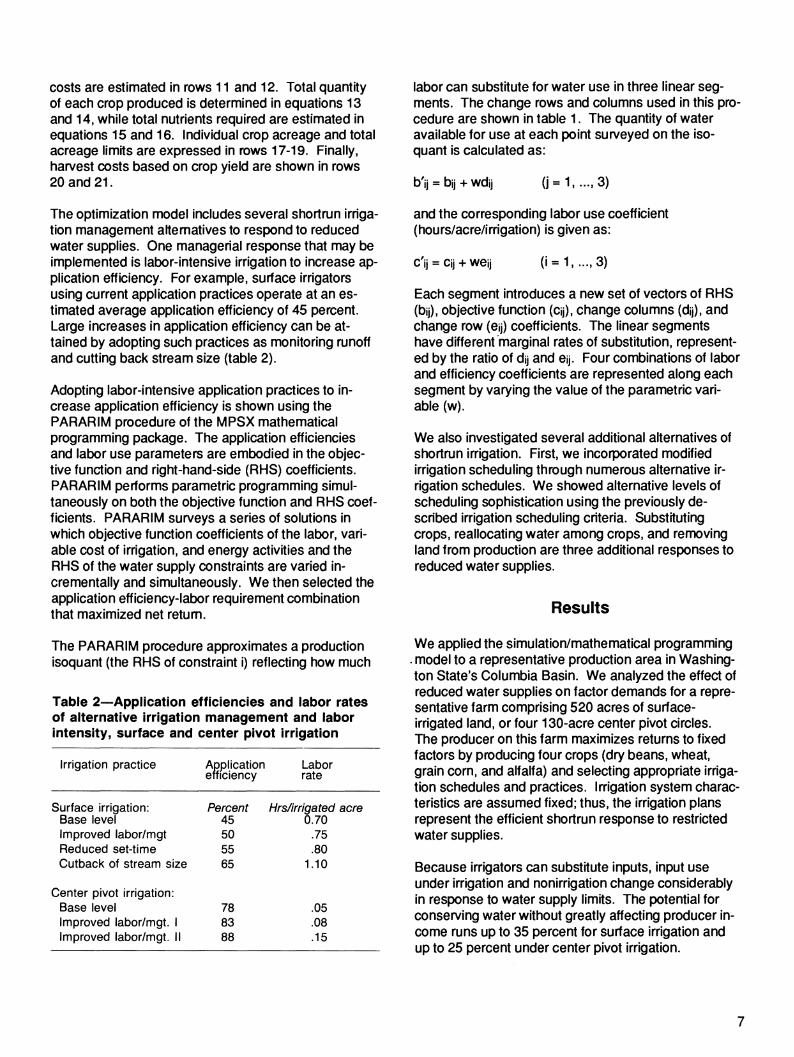
The optimization model includes several shortrun irrigation management alternatives to respond to reduced water supplies. One managerial response that may be implemented is labor-intensive irrigation to increase application efficiency. For example, surface Irrigators using current application practices operate at an estimated average application efficiency of 45 percent. Large increases in application efficiency can be at- tained by adopting such practices as monitoring runoff and cutting back stream size (table 2).

Adopting labor-intensive application practices to increase application efficiency is shown using the PARAR IM procedure of the MPSX mathematical programming package. The application efficiencies and labor use parameters are embodied in the objective function and right-hand-side (RHS) coefficients. PARARIM performs parametric programming simultaneously on both the objective function and RHS coefficients. PARARIM surveys a series of solutions in which objective function coefficients of the labor, variable cost of irrigation, and energy activities and the RHS of the water supply constraints are varied in- crementally and simultaneously. We then selected the application efficiency-labor requirement combination that maximized net return.

The PARARIM procedure approximates a production isoquant (the RHS of constraint i) reflecting how much

Table 2—Application efficiencies and labor rates of alternative irrigation management and labor intensity, surface and center pivot irrigation

Irrigation practice Application efficiency

Labor rate

Surface irrigation: Base level

Percent 45

Hrs/irrigated acre 0.70

Improved labor/mgt Reduced set-time

50 55

.75

.80 Cutback of stream size 65 1.10

Center pivot irrigation: Base level 78 .05 Improved labor/mgt. 1 Improved labor/mgt. II

83 88

.08

.15

labor can substitute for water use in three linear segments. The change rows and columns used in this procedure are shown in table 1. The quantity of water available for use at each point sun/eyed on the isoquant is calculated as:

b'ii = bii + wdi ij ^u (j=1.....3)

and the corresponding labor use coefficient (hours/acre/irrigation) is given as:

c ¡j = Cij + weij (i = 1 3)

Each segment introduces a new set of vectors of RHS (bij), objective function (c¡j), change columns (dij), and change row (eij) coefficients. The linear segments have different marginal rates of substitution, represented by the ratio of dij and eij. Four combinations of labor and efficiency coefficients are represented along each segment by varying the value of the parametric variable (w).

We also investigated several additional alternatives of shortrun irrigation. First, we incorporated modified irrigation scheduling through numerous alternative irrigation schedules. We showed alternative levels of scheduling sophistication using the previously de- scribed irrigation scheduling criteria. Substituting crops, reallocating water among crops, and renx)ving land from production are three additional responses to reduced water supplies.

Results

We applied the simulation/mathematical programming . model to a representative production area in Washing- ton State's Columbia Basin. We analyzed the effect of reduced water supplies on factor demands for a representative farm comprising 520 acres of surface- irrigated land, or four 130-acre center pivot circles. The producer on this farm maximizes returns to fixed factors by producing four crops (dry beans, wheat, grain corn, and alfalfa) and selecting appropriate irrigation schedules and practices. Irrigation system characteristics are assumed fixed; thus, the irrigation plans represent the efficient shortrun response to restricted water supplies.

Because Irrigators can substitute inputs, input use under irrigation and nonirrigation change considerably in response to water supply limits. The potential for conserving water without greatly affecting producer income runs up to 35 percent for surface irrigation and up to 25 percent under center pivot irrigation.

The effect of reduced water supply on labor demand depends on the type of irrigation system used. Adopt- ing high-frequency schedules by center pivot Irrigators demands significantly more labor as water supply is reduced.

Surface Irrigators, on the other hand, initially see a decrease in labor required, but further water supply reductions do raise labor demand.

Surface Irrigation

Table 3 summarizes results for six annual water supply allotments applied to the surface-irrigated farm. Producers are assumed to have complete flexibility in allocating available water over the imgation season. Restrictions on water supply might be those imposed by some regulatory body or from voluntary forfeiture of a portion of a water right.

Under an optimal irrigation management plan, when water supply is unlimited, an annual water supply of 26,884 acre-inches is used to generate a return to land, management, and fixed costs of $84,462 (table 3, column 1 ). Of the total quantity of water applied, 12,098 acre-inches are made available for net irrigation, and a total of 13,286 acre-inches of water are used consumptively by the four crops. Since total consumptive use (as measured by actual évapotranspira- tion) exceeds net irrigation, rainfall and initial soil moisture provide a portion of crop water used.

The most optimal in^igation schedules were high water- use schedules which resulted in crop yields approach- ing the maximum attainable. Under sufficient water availability and low irrigation costs, profit-maximizing

yields approach the maximum attainable (table 4, column 1).

Water supplies are reduced using a combination of alternative water consen/ation practices discussed ear- lier. By scheduling imgations to correspond to crop water demands and by adopting practices to minimize irrigation losses, initial water restrictions are met with little effect on crop consumptive use. Total annual crop consumptive use is reduced less than 4 percent in meeting an 18-percent reduction (from 26,884 to 22,000 acre-inches) in the total quantity of water applied. This result would indicate a reduction in water application from Wm to W in figure 1. Crop consumptive use becomes an increasingly large percentage of incremental reductions in water allotments below 22,000 acre-inches. For example, reduced consumptive use accounts for over half of the decrease in the quantity of water applied in nx)ving from a 16,000 acre- inch allotment to a 12,000 acre-inch allotment (table 4). Yields drop between 6 and 17 percent from maximum in meeting the most limiting water supply allotment. These reductions approximately translate to a 27-percent decline in net retums.

All 520 acres of available land remain in production until the water supply is reduced the final time. Thus, water applications can be reduced more than 40 percent before a reduction in acreage will decrease net returns more than a further reduction in the irrigation depth of one or more crops. This result reflects both a low marginal productivity of applied water over this range of water supply and a high marginal contribution of an acre of irrigated land to farm level net returns. Barrett and SkogertDoe's findings may be supported by this result. They state, "the optimal irrigation policy is to apply water quantities consistent with maximum

Table S—lnputs required for alternative annual water allotments on a 520-acre surface-irrigated farm

Annual water allotment (acre -inches) Item Unit

26,884 25,000 22,000 19,000 16,000 12,000

Net returns Dollars 84,462 84,244 82,352 79,745 76,749 61,336 Net irrigation Acre-inches 12,098 11,250 10,560 10,450 8,800 7,800 Consumptive use Acre-inches 13,286 12,990 12,715 11,910 10,812 8,714 Application efficiency Percent 45 45 45 55 55 65 Labor requirement^ Hours .70 .70 .73 .80 .80 1.10 Land Acres 520 520 520 520 520 475 Labor (total) Hours 4,374 4,190 3,950 3,670 3,700 4,040 Nitrogen Tons 34.2 34.0 32.3 30.9 28.6 22.1

1 Hours of irrigaton labor required per acre for each irrigation.

yield only if application efficiencies are high; if efficiencies are low, less water should be applied" ( 1). The lower the efficiency, the lower the marginal contribution of applied water to crop yield, and the more that irrigation can be reduced as necessary.

Reduced nutrient requirements accompanying reduced water supplies follow a pattern similar to crop consumptive use. Nitrogen applications are reduced only 3.3 tons (less than 10 percent of the full-yield requirement) in meeting the 19,000-acre-inch annual water allotment. However, in attaining an additional 26-percent reduction in water supply (from 19,000 to 12,000 acre- inches), farm-level nutrient use is decreased 26 percent below the full-yield nutrient requirement. This nutrient reduction reflects both a decrease in the rate of nitrogen application to planted crops, and a decrease in irrigated acreage. Nutrient demand should show a similar level of sensitivity to water supplies reduced below 12,000 acre-inches.

Labor and application efficiency coefficients presented in table 3 demonstrate the effects of adopting efficiency-increasing, labor-intensive irrigation practices as water use is nrx)re constrained. Labor-water substitution is shown in figure 3. The isoquants shown are iso-net revenue curves derived from a series of solutions of the two-stage model. The slope of the isocost line represents the negative of the ratio of the

shadow price of water to the hourly wage rate. The optimal solution for an annual water supply of 22,000 acre-inches is represented at point A. Net returns of $82,352 are earned by combining 22,000 acre-inches of water with 3,950 annual labor hours. When the water supply is reduced to 16,000 acre-inches, water's shadow price (implicit price) increases, which increases the absolute value of the slope of the isocost line.

Labor is substituted for the scarce water input by monitoring runoff and reducing set-time, increasing application efficiency by 7 percent and labor required by 0.07 hour/acre/imgation. An annual labor requirement of 3,700 hours is used in conjunction with 16,000 acre- inches of water to generate $76,749 of net returns (point B). We show optimal adjustments to reducing the allotment to 12,000 acre-inches by a movement from B to C where net revenue is $61,336. An expansion path representing the points where labor use is most efficient for producing each level of total revenue is labeled EP*.

Changes in farm-level labor in response to reduced water supplies exhibit some interesting characteristics. We initially reduce the water supply by decreasing the frequency of im'gation and thus decreasing labor use. Total labor use is reduced 16 percent below that required to apply the base-level water allotment in order

Table 4—Individual crop information for alternative annual water allotments on a 520-acre surface- irrigated farm

Crop Unit Annual water allotment (acre-inches)

26.884 25,000 22,000 19,000 16,000 12,000

Dry beans: Average water applied Average yield

Acre-inches Cwt/acre

39.6 23.9

39.6 23.9

37.1 23.9

30.1 23.1

26.9 22.6

19.5 20.9

Grain corn: Average water applied Average yield

Acre-inches Tons/acre

54.5 4.77

54.5 4.77

44.1 4.49

37.4 4.39

37.4 4.39

32.3 4.39

Wheat: Average water applied Average yield

Acre-inches Bushels/acre

45.3 89.8

45.3 89.8

42.6 89.8

38.2 89.8

24.9 80.6

16.9 76.8

Alfalfa: Average water applied Average yield

Acre-inches Tons/acre

67.5 6.46

52.9 6.23

45.2 6.16

40.4 6.16

40.4 6.16

35.0 6.16

Note: All crop acreages are 130 acres, except grain corn which is 85 acres in the 12,000-acre-inch solution.

to meet the 19,000-acre-inch allotment. However, as Ir- rigators adopt more labor-intensive application practices to meet restricted water supplies, total labor required begins to increase. The annual imgation labor required increases nearly 400 hours in moving from the 19,000- to the 12,000-acre-inch allotment. This result primarily reflects the increase in labor intensity of 0.3 hour/acre/irrigation required to attain a 10-percent increase in application efficiency.

Failure to incorporate those irrigation practices which increase application efficiency seriously understates an irrigator's ability to meet water supply reductions. An expansion path assuming a fixed labor-application efficiency ratio (0.70/0.45) is illustrated in figure 3 as EP'. The discrepancy between fixed and variable efficiency solutions can be illustrated by comparing the net returns associated with a 16,000-acre-inch water supply. The annual loss in income would be understated $8,000 and labor use, 850 hours, if the possibility of substituting labor for water was not considered. This difference between fixed and variable application efficiency solutions becomes more pronounced as water supply becomes more limited.

Center Pivot Irrigation

Table 5 summarizes the required inputs for five alternative annual water allotments to the center pivot irriga-

ted farm. We used all assumptions in the surface in'igation scenario, except for the prevailing irrigation technology. An unlimited water supply's conditions are represented in the first column; these conditions illustrate the behavior of cun'ent center pivot Irrigators responding to unconstrained water supplies. The profit- maximizing producer, facing low variable costs of irrigation, tends to maximize efficiency of the limiting input-in this case, land. Irrigation schedules selected as optimal are high water-use schedules with nearly the maximum attainable crop yields.

As in the surface irrigation scenario, Irrigators meet water supply reductions by adopting several irrigation management practices. By reallocating water among crops, monitoring crop water demands, adopting improved irrigation scheduling, and using alternative application practices, reductions in net returns are minimized. Initial water supply reductions are met with little effect on crop consumptive use. Total consumptive use is reduced less than 6 percent in meeting a 28- percent reduction (from 15,208 to 11,000 acre-inches) in the annual water allotment. Water supply reductions below 11,000 acre-inches, in contrast, are met primarily through decreased consumptive use. Because of the high application efficiency of center pivot irrigation, opportunities for reducing irrigation losses are fewer than with surface irrigation methods.

Figure 3

Labor-water substitution with fixed and variable factor ratios under surface irrigation

Labor (100 hours)

40

36

30

25

NR = $ 82.300

NR = $ 76,700

'NR = $68.000

NR = $61.300

J \ \ I \ L

12 16 20 Water

(1.000 acre-inches)

24

10

Irrigated acreage is removed from production to meet the final two water allotments evaluated. As in the case of surface irrigation, once decreased consumptive use accounts for a large part of water supply reductions, land begins to be idled under efficient seasonal irrigation plans. Acreage is removed from production under center pivot irrigation to meet smaller percentage water supply reductions, and in larger quantities than for surface irrigation. This result reflects the higher marginal productivity of water applied using sprinkler irrigation and is consistent with the relationship between application efficiency and irrigation depth.

Center pivot Irrigators use a water conservation strategy involving high-frequency, deficit irrigation schedules. Imgation scheduling becomes increasingly sophisticated as available water is reduced. For example, irrigations to meet the 8,000-acre-inch allotment are scheduled based on soil moisture percentage and accumulated ET. These schedules maximize the efficiency of water use by applying water quantities corresponding to crop water needs. Adopting high- frequency irrigation schedules essentially substitutes labor for the scarce water resource. The annual irrigation labor required increases approximately 100 percent to meet the most constraining water supply reduction. Restricted water supplies affect labor use (when measured as a percentage of labor demand under unrestricted water availability) more under center pivot irrigation. Surface Irrigators are affected more by limits on water availability in terms of changes in the total labor required.

We assumed water is conveyed to the farm without cost to the Irrigator; thus, the irrigation energy required is limited to the amount needed to pressurize the water for sprinkler application. Changes in annual energy use are few because the Irrigator is limited to shortrun

responses to water supply limits. Energy is reduced 48 percent from 578 megawatt-hours to 304 to meet the water supply reductions evaluated.

Reduced water supplies initially have little effect on farm-level nutrient requirements, as in the case of surface irrigation. Nutrient use is partially based on crop yield. Since initial water supply limits are met with little effect on crop yields, nutrient demands are affected only nominally. Nitrogen demand is somewhat more sensitive to water supplies below 11,000 acre-inches; however, this sensitivity is less than that in the surface irrigation scenario. The alfalfa acreage removed from production in meeting water supply reductions to the center pivot irrigated farm affects total nutrient demand less than when corn acreage is idled in the surface irrigation scenario.

Producers in the study region typically pay a fixed per- acre water charge; therefore, irrigation costs are limited to labor, energy, and repair costs. Results presented in table 5 were based on an energy cost of $0.033 per kilowatt hour (kWh). To analyze the effect of an increase in the marginal cost of water on inputs required, a $0.01 per kWh (31 percent) increase in energy cost was used. Water price changes most affect the optimal plan when water supply is unlimited. Annual water demand drops from 15,208 to 13,227 acre-inches (13 percent) by adopting irrigation practices and schedules to increase the efficiency of water use. An- nual energy required also drops 9 percent. Labor use increases 33 percent over levels reported in table 5 as a result of adopting efficiency-augmenting irrigation schedules. As water supplies are reduced, however, the effects of energy cost increases on the use of other inputs diminished. Input use in response to 9,000- and 8,000-acre-inch allotments changed minimally as a

. result of the increased marginal cost of water.

Table 5—Inputs required for alternative annual water allotments on a 520-acre center pivot irrigated farm

Annual water allotment (acre-inches) Item Unit

15,208 13,000 11,000 9,000 8,000

94,056 93,650 88,162 77,166 70,321 11.862 10,140 9,130 7,470 6,640 13,410 13,291 12,064 10,825 8,334

78 78 83 83 83 .05 .05 .08 .08 .08

520 520 520 502 461 344.5 473.1 645.0 680.3 696.4 577.9 494.0 418.0 342.0 304.0

34.0 33.8 31.7 30.9 29.8

Net returns Dollars Net irrigation Acre-inches Consumptive use Acre-inches Application efficiency Percent Labor required^ Hours Land Acres Labor (total) Hours Energy Megawatt-hours Nitrogen Tons

^Hours of irrigation labor required per acre for each irrigation.

11

Maximum Flow Rates

A second form of restricted water supply occurs when the flow rate of water to the farm is limited, but the total annual water supply is not. Such a condition may reflect a maximum pumping rate, a maximum distribu- tion system capacity, or other limits imposed on daily water availability. We evaluated three limits on the flow-rate available to the center pivot irrigated farm, 4,000,3,000, and 2,000 gallons per minute (gal/min). These flow rates are incremental reductions from the 5,185 gal/min-rate required to optimally distribute an unrestricted water supply (table 6, column 1).

Capacity restrictions have the greatest effect on irrigation decisions during the peak-use period from mid- June to mid-July. Atmospheric demand (as measured by potential évapotranspiration) during this period is at its highest, and wheat, beans, and corn are most sus- ceptible to water stress. Irrigators respond to capacity restrictions with two principal practices: (1) adopting irrigation schedules that shift water use to off-peak periods of the irrigation season, and (2) using high-frequency, low water-use irrigation schedules.

The required inputs and effects on income associated with the three alternative flow-rate restrictions indicate minimal income losses associated with reducing flow rates to 4,000 or 3,000 gal/min. Returns decline less than 1 percent to meet the 3,000 gal/min allotment. The effects on income resulting from a 2,000 gal/min flow rate are more pronounced; this restriction limits

Table 6—Inputs required for alternative capacity restrictions on a 520-acre center pivot irrigated farm

Capacity (fjgw-rate) restriction (gal/min )

Item Unit Unlimited 4,000 3,000 2,000

Net returns Dollars 94,056 93,959 93,352 79,880 Applied water Acre-inch 15,208 14,259 13,077 11,141 Net irrigation Acre-inch 11,862 11,122 10,200 8,832 Consumptive

use Acre-inch 13,410 13,382 13,011 11,988 Application

efficiency Percent 78 78 78 83 Labor

requirement^ Hours .05 .05 .05 .08 Land Acres 520 520 520 520 Labor (total) Hours 344.5 391.0 443.4 488.5 Energy Megawatt

hours 577.9 473.4 496.9 423.4 Nitrogen Tons 34.0 33.7 33.0 28.9

1 Hours of irrigation labor required per acre for each irrigation.

the irrigator's ability to redistribute water over the irrigation season to avoid significantly lower crop yield.

Capacity restrictions have a pronounced effect on all three measures of water use (total water applied, net irrigation, and crop consumptive use). Reductions of 6 and 14 percent in both applied water and net irrigation result with flow rates of 4,000 and 3,000 gal/min. Ir- rigators facing a more restrictive flow rate of 2,000 gal/min reduce water use more significantly; in this case, applied water and net irrigation are reduced 30 and 26 percent. Total consumptive use is reduced 4,578 acre-inches (23 percent) to meet the 2,000 gal/min flow-rate restriction. Capacity restrictions also affect the timing of water demand. To meet the 2,000 gal/min restriction, water demand during the peak-use period of June 15 to July 15 is reduced 34 percent below the quantity applied in the unconstrained solution.

Annual labor required increases monotonically as flow rate is restricted when high-frequency irrigation schedules are used to meet flow-rate restriction. Total annual labor use increases 144 hours (42 percent) over the range of capacity constraints evaluated. This increase results primarily from the high-frequency irriga tion schedules used to meet the 2,000 gal/min capacity constraint. Annual energy required decreases 27 percent to meet the 2,000 gal/min capacity limit due to the reduced quantity of water applied. The total annual nitrogen required decreases 12 percent.

Conclusions

Water availability principally determines the relative combination of land and water used in irrigation. Only minor reductions in acreage resulted as Irrigators responded to water quantity and price changes in this analysis. Irrigators can manage reduced water supplies by increasing the efficiency of water use through other factors (such as labor) rather than removing land from production. Land seldom limits production in areas where crop production depends on irrigation.

Because Irrigators can substitute inputs, input use under irrigation and nonirrigation change considerably in response to water supply limits. Nutrient use corresponds closely with reduced crop use. Nutrient applications decrease nominally in response to initial water reductions, but increase with more limited water supplies.

The effect of reduced water supply on labor demand depends on the type of irrigation system used. Center pivot Irrigators' adoption of high-frequency irrigation

12

schedules demands significantly more labor as water supplies are limited. Surface imgators, on the other hand, see a decrease in labor required with initial water reductions, but further water reductions result in increases in labor demand. Water and energy are combined in fixed proportions; thus, reduced energy use closely corresponds with reduced water supply. Inputs demanded under reduced water supplies depend on prices and regional availability.

Our results also indicate that water in irrigated agriculture can be conserved significantly with only small tos- ses in producer income. This potential runs up to 35 percent for surface irrigation and up to 25 percent under center pivot irrigation. Surface in^igators' ad- vantage in responding to water supply deficits reflects the system's low base-level efficiency and opportunities to use efficiency-augmenting application practices. Opportunities to conserve water were substantial over the range of economic and resource conditions investigated.

Labor and capital can frequently substitute for water. Efficiency of water use is determined by the relative scarcity of water and the value of the irrigated crop.

References

1. Barrett, J.W., and Gaylord V. Skogertx)e. "Crop Production Functions and the Allocation and Use of Ir- rigation Water." Agriculture Water Management, 3:53- 64,1980.

2. Bauscher, Lonny D., Herbert R. Hinman, Elvin L. Kulp, Ladd A. Mitchell, John L. Moore, and Gary 0. Pel- ter. 1984-85 Cost of Producing Crops Under Center Pivot Irrigation, Columbia Basin, Washington. Ext. Bull. No. 1291, Coop. Ext. Serv., Washington State University, Pullman, WA, 1984.

3. Bernardo, Daniel J. "Optimal In-igation Manage- ment Under Conditions of Limited Water Supply." Un- published Ph.D. dissertation, Dept. of Agricultural Economics, Washington State University, Pullman, WA, 1985.

_, N.K. Whittlesey, K.E. Saxton, and D.L. Bas- 4. _ sett. "An Irrigation Model for Management of Limited

Water Supplies." Western Journal of Agricultural Economics, 12(2) :164-173,1987.

5. Doorenboos, J., and A.J. Kassam. "Yield Response to Water." Rome: United Nations Food and Agricul- ture Organization, Irrigation and Drainage Paper No. 33,1979.

6. Hanks, R.J. "Model for Predicting Plant Yield as In- fluenced by Water Use," Agronomy Journal, 66 (3): 660-665,1974.

7. Hillel, D. "The Field Water Balance and Water Use Efficiency." Pp. 79-100 in Optimizing the Soil Physical Environment Toward Greater Crop Yield. D. Hillel, ed. Academic Press, New York, 1972.

8. Houston, Jack E., and N.K. Whittlesey. Modeling Ir- rigation in the Columbia, State of Washington Water Resources Center, Report 65, June 1985.

9. Jensen, Man/in E. "Water Consumption by Agricul- tural Plants." Pp. 1-22 in Water Deficits in Plant Growth, vol. 2. T.T. Kozlowski, ed. Academic Press, New York, 1968.

10. Saxton, Keith E. "Mathematical Modeling of Evapotranspiration on Agricultural Watersheds." Pp. 183-204 in Modeling Components of the Hydrologie Cycle, Proceedings of the International Symposium on Rainfall-Runoff Modeling, Mississippi State University Water Resources Publications, Mississippi State, 1981.

11. , H.P. Johnson, and R.H. Shaw. "Modeling Evapotranspiration and Soil Moisture." Trans American Society of Agricultural Engineering, 17(4) :673-77,1974.

12. Stewart, J. Ian, and Robert M. Hagan. "Functions to Predict Effects of Crop Water Deficits." Journal of the Irrigation Drainage Division, American Society of Civil Engineering, 99 (IR4):421-439,1973.

13. Sudar, Robert A., K.E. Saxton, and R.G. Sponer. "A Predictive Model of Water Stress in Corn and Soybeans." Trans American Society of Agricultural En- gineering, (24): 97-102,1981.

13

^'U.S. GOVtRNWENT PRINTING Orr ICE :l9a9-241-852 : 0Q211/LR5

Keep Up-To-Date on Agricultural Resources. Subscribe to the Agricultural Resources Situation and Outlook report and receive timely analysis and forecasts directly from the Economic Research Sen/ice. Subscription includes five issues, each devoted to one topic, including farm inputs, agricultural land values and markets, water, and conservation. Save money by subscribing for more than 1 year.

Agricultural Resources Situation and Outlook Subscription

Domestic

Foreign

1 Year _ $10.00

2 Years _ $19.00

3 Years _ $27.00

$12.50 $23.75 .$33.75

For fastest service, call toll free,

1-800-999-6779 (8:30-5:00 ET)

I I Bill me. [^ Enclosed is $

Credit Card Orders :

I I MasterCard [^ VISA Total charges $_

Use purchase orders, checks drawn on U.S. banks, cashier's checks, or international nrKDney orders. Make payable to ERS-NASS.

Credit card number: Expiration date: Month/Year

Name

Address

City, State, Zip.

Daytime phone (_

Mail to:

ERS-NASS P.O. Box 1608 Rockville, MD 20850

í/f^ ¿dl^ ^'^^koa factor demand in

Documents