extreme wet years over southern africa: role of indian ...blyon/references/p65.pdf · extreme wet...

Extreme wet years over southern Africa: Role of Indian Ocean sea

surface temperatures

Richard Washington1 and Anthony Preston1

Received 30 September 2005; revised 16 March 2006; accepted 2 May 2006; published 8 August 2006.

[1] Southern Africa is a predominantly semiarid region with a high degree of interannualrainfall variability. Although much of the recent climate research has focused on thecauses of drought events, the region has also experienced extremes of above averagerainfall, the most recent examples being the major flooding episodes that devastatedMozambique during 2000 and 2001. This paper investigates extremely wet years oversouthern Africa during the twentieth century. Focusing on the two most extreme years,1974 and 1976, we show that while ENSO serves as an important control on rainfallvariability, a specific pattern of SSTs in the SW Indian Ocean, with warm anomalies inthe subtropical SW Indian Ocean and cool anomalies in the northern SW Indian Oceanthat is statistically independent of ENSO, plays a crucial role in generating extremeconditions. To do this, we use a series of multimodel experiments, to demonstrate first theimportance of global sea surface temperatures. Through additional idealized experimentswith HadAM3, we then isolate the role of SST anomalies in the Indian Ocean. Theanomalies are based on the observed SSTs with the ENSO signal linearly removed. Thecritical influence is tied to cold SST anomalies in the Mascarene region which inducean anomalous anticyclonic circulation driving an anomalous low-level easterly moistureflux along 10–20�S into eastern southern Africa. This results in enhanced moistconvective uplift, conducive to enhanced rainfall, over a large part of southern Africa.Near surface humidity and 500-hPa omega fields extend from eastern southern Africa intothe Agulhas region in a tropical-temperate cloud band like structure. The similaritybetween the reanalysis fields for the extreme years and the model experiments is striking.

Citation: Washington, R., and A. Preston (2006), Extreme wet years over southern Africa: Role of Indian Ocean sea surface

temperatures, J. Geophys. Res., 111, D15104, doi:10.1029/2005JD006724.

1. Introduction

[2] Southern Africa is a predominantly semiarid regionwith a high degree of interannual rainfall variability [Tyson,1986; Mason and Jury, 1997]. A heavy reliance on subsis-tence agriculture exposes the population base to droughtevents [Vogel, 1994; Mason and Joubert, 1995; Washingtonand Downing, 1999; Dube and Jury, 2000; Jury, 2002], afeature of the climate system which has received significantrecent emphasis [e.g., Cook, 2001; Jury, 2002; Jury andMwafulirwa, 2002; Endfield and Nash, 2002; Nash andEndfield, 2002; Levinson, 2004; Thomson et al., 2003;Usman and Reason, 2004]. The increased likelihood ofthe greater frequency and intensity of sustained drought[Hoerling et al., 2006], land degradation and desertification[Thomas and Leason, 2005; Thomas et al., 2005] in futuredecades, set against the pressure of increasing population,further raises the vulnerability of this region.

[3] In addition to the hazard of drought, southern Africahas also experienced extremes of above average rainfall, themost recent examples being the major flooding episodesthat devastated Mozambique during 2000 and 2001 duringwhich hundreds of people were killed and nearly 200,000people made homeless. Total cost of the damage resultingfrom the 2000 event was approximately 500 million USD[du Plessis, 2002]. In parts of southern Africa, an increasedfrequency of heavy rainfall events has been identified overthe period 1979–2002 [Usman and Reason, 2004]. Overallthere is somewhat less research on wet events over southernAfrica (examples include Mason and Joubert [1997] andReason and Keibel [2004]).[4] A more complete understanding of climate mecha-

nisms in southern Africa can only come about if both wetand dry years are considered. Accordingly, this paperinvestigates years of large rainfall excess over southernAfrica. In particular, we are concerned with the sea surfacetemperature (SST) patterns and their associated atmosphericcirculation anomalies that accompany wet extremes. Thepaper examines the hypothesis that Indian Ocean SSTanomalies are crucial for explaining extremely wet years.Section 2 presents an analysis of observed rainfall and seasurface temperatures associated with years of extreme

JOURNAL OF GEOPHYSICAL RESEARCH, VOL. 111, D15104, doi:10.1029/2005JD006724, 2006ClickHere

for

FullArticle

1Climate Research Lab, Oxford University Centre for the Environment,University of Oxford, Oxford, UK.

Copyright 2006 by the American Geophysical Union.0148-0227/06/2005JD006724$09.00

D15104 1 of 15

http://dx.doi.org/10.1029/2005JD006724

rainfall. Experiments with atmosphere climate models drivenwith historical SST and idealized SST patterns are examinedin section 3. Section 4 provides a discussion and summaryof the main findings.

2. Observed Rainfall and Sea SurfaceTemperatures

2.1. Background

[5] Southern Africa south of 15�S is a predominatelysemiarid region. Annual rainfall totals averaged over landsouth of 15�S are 316 mm.yr�1, with 40% of the totalrainfall occurring between January and March, associatedwith the southward migration of tropical convection to thesubtropical latitudes (approximately 20�S) and the forma-tion of tropical-temperate cloud bands at this time of year[Mason and Jury, 1997; Washington and Todd, 1999].

2.2. Rainfall Variability

[6] We start with the time series of area average land-based rainfall anomalies for southern Africa south of 15�S(Figure 1) for 1900 to 1998. The area average for each JFM(January, February, March) season was calculated from themean of rainfall anomalies (based on 1961–1990 period)using the Hulme et al. [1998] monthly data set (2.5�latitude � 3.75� longitude resolution). Three years in therecord of area average rainfall exceed 2.5 standard devia-tions above the mean (1976, 1974 and 1909). The two mostextreme years fall into the latter half of the twentieth centuryduring which meteorological and oceanographic records areof sufficient quality to support detailed analysis. In thisstudy, we therefore focus on the JFM season of 1976 and1974, neither of which has been comprehensively studiedbefore.

2.3. ENSO and Anomalously Wet Years

[7] One simple explanation for the extreme rains in 1974and 1976 lies with the ENSO phenomenon. It has long been

known that southern African summer rainfall is significantlyinfluenced by ENSO [Lindesay, 1988; Van Heerden et al.,1988; Ropelewski and Halpert, 1989; Nicholson, 1997;Nicholson and Kim, 1997; Cook, 2000, 2001] with La Ninaepisodes generally bringing anomalously wet conditions(Figure 2). This association is also evident in at least 200years of proxy and observed data [Lindesay and Vogel,1990], although the strength of the relationship has variedover the past century. Table 1 confirms that for each of themonths January through March 1974 and 1976, extreme LaNina conditions prevailed in the Pacific. During each ofthese months in 1974, the Southern Oscillation Index (SOI)was the highest value recorded throughout the period 1950to 1998 inclusive. Likewise, 1976 was ranked the 5thhighest SOI in January and February and the 3rd highestin March. The Nino3 SST rankings are similarly extreme.[8] However, a clear indication that Pacific sea surface

temperature conditions are not a simple determinate ofanomalously wet conditions over southern Africa, is thatother years with anomalously cool Nino3 SSTs between1950 and 1998, some of which rank higher than 1976 inwidely used ENSO indices (including SOI and Nino3), werenot anomalously wet. Examples include 1968, which wasanomalously dry and 1970/1971, a near averageyear. Likewise, 1967/1968 featured an extreme La Nina.Conditions were predominately wet over southernAfrica but at 0.55 standard deviations above the mean,not excessively so.

2.4. Non-ENSO Related Rainfall Variability

[9] A key question relating to the two extreme rainfallyears of 1974 and 1976 is whether these years were simplya result of unusually strong La Nina events or whether otherconditions, in addition to and perhaps independent of, theLa Nina events were favorable for above normal rainfall.The existence of extreme La Nina years which werenot excessively wet (and some of which were dry) over

Figure 1. Southern African January to March (JFM) rainfall south of 15�S from the Hulme et al. [1998]data set, 1900–1998. Vertical axis shows standardized anomalies relative to the 1961–1990climatological mean (mean is 316 mm and standard deviation is 80 mm).

D15104 WASHINGTON AND PRESTON: EXTREME WET YEARS IN SOUTHERN AFRICA

2 of 15

D15104

southern Africa (section 2.3) suggests that other influencesmay also control rainfall and there is indeed much in theliterature to suggest that SSTs in surrounding ocean basinsexert an independent influence on southern African rain-fall [Walker, 1990; Rocha and Simmonds, 1997a, 1997b;Goddard and Graham, 1999; Behera and Yamagata, 2001;Reason, 2002]. It is also clear that ENSO controls much lessthan half of the interannual variance of JFM SSTs in theIndian Ocean (Figure 3).[10] To test the possible role of non-ENSO influences, we

create an index of southern African rainfall with ENSOlinearly removed by regression. Although there are anumber of limitations to this technique, most notably thoserelating to linearity, it does provide a basic way of analyzingvariability independent from ENSO and has been used in anumber of previous studies for the same purpose [e.g.,Jones, 1988, 1994; Christy and McNider, 1994; Zhang etal., 1996; Kruger, 1999; Barreiro et al., 2002]. Regressionwas favored over the use of bandpass filtering. In the lattertechnique, removal of the interannual component of vari-ability (2–7 years), which characterizes ENSO, would havealso resulted in the removal of non-ENSO modes ofvariability on similar timescales.

[11] The regression approach used to linearly removeENSO may be formalized as follows:

yi ¼ bþ a xi ð1Þ

y0i ¼ yi � yi ð2Þ

where

yi = Seasonal (JFM) rainfall anomaly (with reference to1961–1990)

xi = Seasonal average ENSO index value

Figure 2. Correlations between JFM Southern Oscillation Index and JFM southern African rainfall for1900–1998 (shaded regions significant at 5% level).

Table 1. ENSO Statistics for January, February and March 1974

and 1976

January February March

1974 SOI 4.3 3.2 3.6Rank 1974 SOI 1950–1998 1 1 11976 SOI 2.4 2.6 2.2Rank 1976 SOI 1950–1998 5 5 31974 Nino 3 �1.64 �1.20 �0.70Rank 1974 Nino 3 1950–1998 1 4 61976 Nino 3 �1.78 �0.97 �0.59Rank 1976 Nino 3 1950–1998 3 6 9


3 of 15

D15104

a = Regression coefficientb = Regression coefficientyi = Estimated value for yi given xiy0i = Seasonal (JFM) rainfall value with ENSO signal

removed

such that each rainfall grid box has a unique regressionequation.

[12] With the ENSO signal linearly removed from eachgrid box of JFM rainfall over southern Africa, we constructthe area average time series of the y’i anomalies using thesame method by which data in Figure 1 were generated(section 2.2).[13] We have investigated the sensitivity of the linear

regression approach to the precise index of ENSO used inthe regression, including OND and JFM averages of theNino3.4, Nino3, SOI and a multivariate index [Wolter andTimlin, 1993] over the period 1950–1998. The rankings ofthe top 8 wet years are not changed as a function of theindex used and we conclude that the results are largelyinsensitive to the precise ENSO index.[14] Even with ENSO linearly removed, both 1974 and

1976 appear as extreme wet anomalies with 1974 as thethird and 1976 the fourth wettest JFM anomalies in the inthe y0i time series from 1900 to 1998. While noting theassumptions of linearity in the regression based approach,we conclude that the extremely wet years of 1974 and 1976may not have been solely a product of Pacific based ENSOforcing.[15] An important caveat in this method and the conclu-

sion we have reached above is that we have not considered

the multidecadal variability of ENSO and the impact thismay have on the Indian Ocean and southern Africa [e.g.,Reason and Rouault, 2002; Allan et al., 2003] in thismethod. The method may also not deal adequately withthe differences between protracted and shorter ENSO events[Allan et al., 2003] which may turn out to be important inthe reasons for the wet conditions in the 1970s.

2.5. Extreme Rainfall and SSTs

[16] In order to establish non-ENSO related SST patternsassociated with the extreme rainfall years of 1974 and 1976,we derive JFM composites of SST anomalies for oceanbasins surrounding southern Africa. We use the Global Iceand Sea Surface Temperature data (GISST2.3b) [Rayner etal., 1996], but prior to computing the composites, welinearly regress the ENSO signal from each grid box (2.5�latitude � 3.75� longitude resolution) of the SST data, usingthe SOI as a measure of ENSO, following the methoddescribed for linearly removing the ENSO signal fromrainfall in section 2.4.[17] Anomalous SST gradients with positive (negative)

anomalies approaching 1�C (�1�C) in the subtropical(tropical) southwest Indian Ocean are clearly evident inthese resulting composites (Figure 4). There are also years,namely 1970 and 1964, where anomalous SST gradients ofthe opposite sign are clearly evident (Figure 5). These years,1970 and 1964 are the second and sixth driest in the y0i timeseries from 1900 to 1998. During 1970, Zimbabwe wasseriously affected by intense drought [Jury et al., 1992].What emerges from this simple statistical analysis, is apattern of SST variability in the SW Indian Ocean with anenhanced poleward gradient associated with some extreme

Figure 3. Correlation (r) between the JFM SOI and JFM SSTs (1959–1998). Shading indicatessignificance at the 5% level. Contour interval 0.1. Interannual variance in JFM SSTs explained by ENSOas measured by the SOI is determined by r2.


4 of 15

D15104

dry years and a relaxed poleward gradient associated withsome extreme wet years.

3. Model Experiments

[18] In section 2 we have shown that the wet years of1974 and 1976 were associated with anomalous SSTpatterns in the southwest Indian Ocean and also with strongLa Nina conditions. To evaluate whether the associationwith the SST patterns was simply coincidental, and if not, totest whether the rains could have resulted from IndianOcean SSTs separate from a Pacific based ENSO influence,we present the results of several atmosphere general circu-lation model (AGCM) experiments.

3.1. Historical SST Experiments

[19] In this section we assess the 1974 and 1976 JFMrainfall anomalies over a broad southern African domainfrom the ensemble mean of 5 atmospheric GCMs forcedwith historical SSTs (Figure 6). These years have beensampled from longer integrations of the models, typically

running from 1950 onward, with each member of theensemble integrated from differing initial conditions in thestart years. The models, approximate resolution and numberof members making up the ensemble mean are shown inTable 2.[20] Positive total rainfall anomalies over southern Africa

are found in all 5 models in JFM 1974 and in 4 of the5 models in 1976 (the exception being NSIPP). Theanomalies are generally larger and more spatially coherentin 1974 than 1976, although the rainfall response within oneyear is not the same in any of the models, probably owing todifferences in the basic state of the models. The COLA,CCM3 and NCEP (and NSIPP to a lesser extent) simula-tions all show rainfall anomalies extending from thetropics to subtropical-extratropical margins during 1974.The structure of this anomaly is reminiscent of the tropi-cal-temperature cloud bands (TTCB) that are regarded asthe leading southern African rainfall producing system[Harrison, 1984; Todd et al., 2004]. In all the simulationsand for both 1974 and 1976, dry anomalies are found north,west or northwest of Madagascar in the southwest Indian

Figure 4. Composite JFM SST anomalies for 1974 and 1976 (contour interval 0.1�C). The JFM SOIsignal has been linearly regressed from all data.

Figure 5. Composite JFM SST anomalies for 1964 and 1970 (contour interval 0.1�C). The JFM SOIsignal has been linearly regressed from all data.


5 of 15

D15104

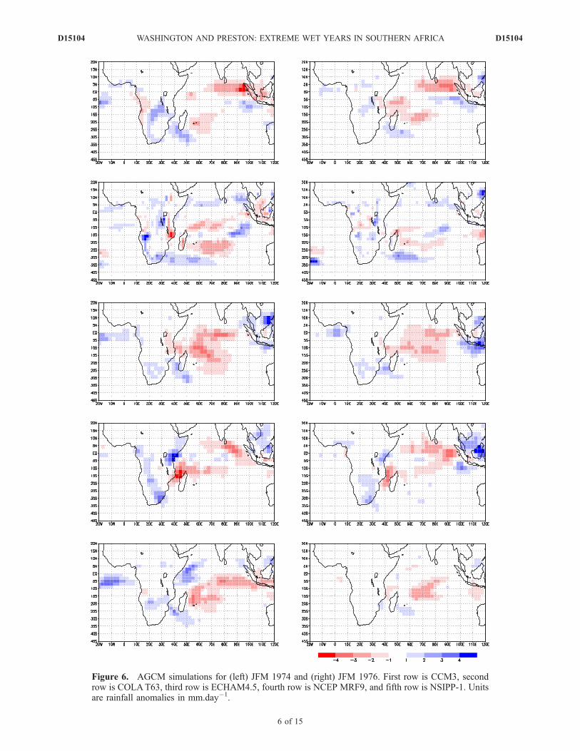
Figure 6. AGCM simulations for (left) JFM 1974 and (right) JFM 1976. First row is CCM3, secondrow is COLAT63, third row is ECHAM4.5, fourth row is NCEP MRF9, and fifth row is NSIPP-1. Unitsare rainfall anomalies in mm.day�1.


6 of 15

D15104

Ocean. The conclusion we reach on the basis of thesesimulations is that the observed global sea surface temper-ature conditions during the austral summer of 1974 and1976 were most likely to have been responsible for gener-ating the anomalously wet conditions over southern Africa.What these experiments are unable to demonstrate iswhether Indian Ocean SSTs could have induced the wetconditions on their own.

3.2. Idealized SST Experiments

[21] We now go on to use idealized sea surface temper-ature experiments with the atmosphere only model,HadAM3, to determine whether the pattern of sea surfacetemperatures evident in the southwest Indian Ocean duringJFM 1974 and 1976 is capable of forcing the anomalouslywet conditions over southern Africa on its own. The experi-

ments are part of a large (>20) suite of experiments usingHadAM3 aimed at an improved understanding southernAfrica rainfall variability and SSTs.3.2.1. Background to HadAM3[22] A large proportion of previous southern African

climate research, including many of the climate changestudies in the mid-1990s, was undertaken using the Com-monwealth Scientific and Industrial Research Organisation(CSIRO) model [Mason et al., 1994; Joubert et al., 1996;Mason, 1996; Mason and Joubert, 1997; Rautenbach andSmith, 2001]. More recently, there have been several sensi-tivity experiments featuring the Melbourne University GCM(MUGCM) [Rocha and Simmonds, 1997b; Reason andMulenga, 1999; Reason, 2001, 2002] and the application ofthe European Centre/Hamburg Model (ECHAM) in the con-text of seasonal forecasting and model output statistics[Landman and Goddard, 2002, 2005]. HadAM3 has beenstudied in the context of intraseasonal [Tennant, 2003] andinterannual variability [e.g., Reason and Jagadheesha,2005], as well as for operational seasonal forecasting.[23] A detailed description of the United Kingdom Mete-

orological Office (UKMO)’s model, HadAM3, is providedby Pope et al. [2000]. In these experiments, the hydro-static model is run in standard climate resolution with ahorizontal grid of 2.5� latitude by 3.75� longitude with 19vertical levels (5 representing boundary layer processes)calculated in hybrid sigma/pressure coordinates [Simmonsand Burridge, 1981].

Table 2. Details of Atmospheric GCMs Used in the Historical

SST Runs

ModelResolution:Latitude

Resolution:Longitude

Number of EnsembleMembers

CCM3 2.8125 2.789328 24COLA C2.2 1.875 1.864678 10ECHAM 4.5 2.8125 2.789328 24NCEP MRF9 2.8125 2.789328 10NSIPP-1 2.5 2.0 9HadAM3 2.5 3.75 6

Figure 7. Idealized SST anomalies (�C) superimposed on the SST climatology to force HadAM3 inexperiment 1. Experiment 2 was forced by the warm anomaly only, and experiment 3 was forced by thecold anomaly only. Climatological SSTs were prescribed in the rest of the global oceans.


7 of 15

D15104

[24] HadAM3 correctly simulates a unimodal annual cyclewith maximum rainfall in the austral summer (October–March) and minimum rainfall in the austral winter (April–September). The model does overestimate summer rainfall.This is most pronounced in the early summer season(October to December) with the positive bias continuinginto the late summer months (January to March). Theannual rainfall total over the whole subcontinent inHadAM3 for JFM is 387 mm compared to the observedtotal of 316 mm. The overall simulation of African climatehas been thoroughly investigated by Preston [2004].3.2.2. Idealized Indian Ocean SST Experiments: Setup[25] In experiment 1, the poleward gradient of SSTs in the

SW Indian Ocean is decreased by imposing a warm SSTanomaly of 1.5�C centered at 32�S, 55�E on the climato-logical SST values and a cold SST anomaly (with aminimum value of �1.0�C) centered at 12�S, 65�E(Figure 7). The location and magnitude of these anomaliesis based on SSTs with ENSO linearly removed during 1974and 1976 (see section 2.5), although the idealized SSTs aresmoothed and symmetrical compared with the observed andSSTs. Also, outside the idealized dipole areas in thisexperiment and in experiments 2 and 3, SSTs over theremaining part of the Indian Ocean follow the climatolog-ical values. In experiment 2 and experiment 3, only thesubtropical warm anomaly and the tropical cold anomalyrespectively are included, so that the role of these separatecomponents of experiment 1 can be considered in isolation.Climatological SSTs are specified in all other parts of theglobal oceans. Each of the experiments has a commondesign, consisting of 10 integrations, which are identicalapart from the arbitrarily different initial starting conditions,thereby allowing for the averaging of internal variability[Mote, 2000; Wehner, 2000]. The SST anomalies are intro-duced in December and are persisted through the latesummer season, although the base SST climatology evolvesaccording to the seasonal cycle with 5-day updates. The

integrations for these experiments all start in November andrun for 5 months until the end of March.[26] The three experiments are evaluated against a control

experiment which consists of 10 years of integrations forcedwith climatological SSTs, starting in April, to give a longspin-up period during which the model is able to reach anequilibrium with the climatological SST forcing beforeanalysis in the late austral summer (JFM) data of thefollowing year. The significance (at the 0.05 level) ofdifferences between the experiments and the control run isdetermined by means of a t-test calculated locally on eachmodel grid box.3.2.3. Idealized Indian Ocean SST Experiments:Results3.2.3.1. Experiment 1[27] Experiment 1, which includes 2 SST anomaly loci in

the SW Indian Ocean, induces large-scale significant atmo-spheric anomalies over southern Africa and the IndianOcean. Positive sea level pressure (SLP) anomalies domi-nate the tropical SWIO, with the peak departures from theclimatology (3 hPa) in the Mascarene region to the east ofMadagascar (Figure 8) representing an equatorward expan-sion of the semipermanent anticyclone and a reduction inthe tropical Indian Ocean SLP minimum (1009 hPa).Accompanying this adjustment are significant anticyclonic850-hPa wind and 700-hPa moisture flux anomalies whichare strongest at 10–20�S, along the northern edge of theSLP anomaly, all but replacing the westerly climatologicalflow in this sector. The effect is to allow the northwardexpansion of the southeasterly trade winds. The significanteasterly 700-hPa moisture flux anomalies (which are repre-sentative of the integrated moisture flux) converge withweaker significant westerly anomalies over Malawi andZimbabwe (Figure 9). This results in significant positive700-hPa specific humidity anomalies (0.5 g.kg�1)and significant negative 500-hPa omega anomalies(�0.02 m.s�1) over eastern southern Africa which extend

Figure 8. JFM SLP anomalies for experiment 1 minus control (contour interval 0.5 hPa). Shadingindicates statistical significance at the 5% level according to a two-tailed Student’s t-test.


8 of 15

D15104

southeast into the Agulhas region as a TTCB form. Whilethe model does not show a significant increase in rainfall,probably because of convective parameterization, the ingre-dients for enhanced rainfall are present.3.2.3.2. Experiment 2[28] Are both the cold and warm components of the SST

anomaly of experiment 1 necessary to bring about theenhanced moisture flux, specific humidity and convectionover southern Africa? On the whole, the SST anomaly inexperiment 2 (warm subtropical component of experiment 1only) appears to have little effect on the large-scale atmo-

spheric circulation over southern Africa and the surroundingocean basins. There are no significant SLP changes inaround southern Africa although there are slight decreases(�0.5 hPa) throughout the southern subtropical IndianOcean and to the south of southern Africa (Figure 10)consistent with a limited weakening and contraction of theSouth Indian High. Associated with these SLP anomalies,there are nevertheless significant northwesterly 850-hPawind anomalies and 700-hPa moisture flux anomalies inthe southeast Indian Ocean which amount to a weakening ofthe southeasterly trade winds There are significant positive

Figure 9. JFM 700 hPa moisture flux anomalies for experiment 1 minus control (scale vector =30 g.kg�1.s�1). Shading indicates statistical significance at the 5% level according to a two-tailedStudent’s t-test.



9 of 15

D15104

humidity anomalies (0.2 g.kg�1) over Lake Malawi and theMozambique Channel with small and nonsignificant posi-tive humidity and negative omega anomalies over the warmSST forcing anomaly.3.2.3.3. Experiment 3[29] Experiment 3, consisting of the cold SST anomaly

component of experiment 1 (in the Mascarene region),generates a response which is very similar to experiment1, especially in the tropical SWIO. There are significantpositive SLP anomalies of a similar magnitude to experi-ment 1 in the Mascarene region to the east of Madagascar

(Figure 11). The 850-hPa wind anomalies and 700-hPamoisture flux anomalies (Figure 12) are also similar be-tween the two experiments. However, there are slight shiftsin the orientation of the anticyclonic feature and the easterlyanomalies along 10�S are slightly weaker in experiment 3compared with experiment 1.[30] Associated with the relatively weaker moisture flux

anomalies, the negative 700-hPa specific humidity anoma-lies in the Mascarene region are weaker in experiment 3than in experiment 1 (�0.9 g.kg�1 compared to�1.5 g.kg�1).The positive 500-hPa omega anomalies are of a similar


Figure 12. JFM 700 hPa moisture flux anomalies for experiment 3 minus control (scale vector =30 g.kg�1.s�1). Shading indicates statistical significance at the 5% level according to a two-tailedStudent’s t-test.


10 of 15

D15104

strength (0.05 m.s�1 compared to 0.06 m.s�1). Overeastern southern Africa, the humidity and omega anoma-lies are of a similar magnitude and location in bothexperiments.3.2.4. Inverse Idealized Indian Ocean SSTExperiments: Experiment 4[31] From the 3 idealized SST experiments, we can

conclude that when HadAM3 is forced with an anomalousSST gradient in the Indian Ocean reminiscent of the SSTanomalies independent of ENSO during 1974 and 1976,circulation features favorable to enhanced rainfall oversouthern Africa result. The model atmosphere’s responseis particularly strong when both the cold and the warm SSTforcing is present, although a similar response results fromthe cold anomaly alone. The role of SST anomalies inforcing the atmosphere can only reasonably be answeredby model experiments, but by their nature, idealized experi-ments impose a substantial separation between the modeland the observed climate system. To be precise, we canconclude that HadAM3 responds to certain SST anomalieswhen the rest of the global oceans are constrained toclimatological SSTs. The idealized SST anomalies are atleast based on statistical analysis of the observed data andare in this sense realistic. However, the anomalies coveronly a small portion of the Indian Ocean while the rest ofthe atmosphere is subjected to forcing by climatologicalSSTs, which is something that never happens in the realworld.[32] It is possible to design an experiment that relaxes this

constraint. Accordingly, in experiment 4, sea surface tem-peratures are permitted to follow their observed values overthe global oceans for the period of integration (1950 to1990), except in that part of the Indian Ocean overlying theregion of the SST anomalies specified in experiment 3. Inthis region, the climatological SST values are specified,with a smoothing relaxing the SSTs to the observed (his-

torical) values at the edges of the region. Experiment 4 thushas varying SSTs everywhere except for the region forwhich the model was shown to be sensitive in experiment 3.[33] To evaluate the experiment, we are looking for a

reduction, relative to a control experiment, in the varianceof the interannual variability of the anomalous 700 hPaeasterly moisture flux over the SW Indian Ocean between10–15�S and 40–60�E. Moisture flux in this area haspreviously been found to control the strength and frequencyof TTCBs over southern Africa [Todd and Washington,1999]. We chose this criterion since it is a characteristicresponse of HadAM3 to the SSTs in experiments 1 and 3.Note that the control experiment in this case is necessarilydifferent from that in experiments 1 through 3 and is anintegration from 1950 to 1990 with historical SSTs over theentire global oceans.[34] The results of experiment 4 show that the variance of

700 hPa moisture flux in the control run is 3.5 times thevariance of the experiment over the SW Indian Ocean box.Over southern Africa itself south of 20�S, moisture flux is4 times higher in the control run. Experiment 4 thereforeconfirms, in an inverse sense, the sensitivity of the modelatmosphere to SST anomalies in the Mascarene region.However, it does this in a way that is less constrained thatexperiments 1 and 3.

4. Summary and Discussion

4.1. Summary of Observed and Model Results

[35] From the analysis of observed southern Africansummer rainfall and SSTs, a clear pattern of SW IndianOcean SSTs linearly independent from ENSO characterizedby warm anomalies in the subtropical SW Indian Ocean andcool anomalies in the northern SW Indian Ocean wasassociated with the two wettest years of the twentiethcentury. It is likely that the effects of strong La Nina eventsin 1974 and 1976 were additive to effects of the SW Indian

Figure 13. Correlation between JFM southern African rainfall and JFM SLP 1959–1998. Shadingindicates statistical significance at the 5% level. SLP data are from the NCEP/NCAR reanalysis data set.The JFM SOI signal has been linearly regressed from all data prior to the calculation of the correlations.


11 of 15

D15104

Ocean SSTs. From a series of multimodel experiments, wehave shown that global sea surface temperatures werecapable of generating anomalously wet conditions oversouthern Africa in those years. Additional experiments withHadAM3 indicate that an idealized pattern of SSTs whichisolate the role of anomalies in the Indian Ocean, based onthe observed SSTs with the ENSO signal linearly removed,is capable of forcing a model response conducive to rainfall.ANOVA testing indicates that approximately 40% of thesignificant circulation response (700 hPa moisture flux overthe SW Indian Ocean box and over eastern southern Africa)is due to the anomalous SST forcing (experiments 1 and 3),a figure that is in broad agreement with studies pointing tothe importance of tropical SSTs in atmospheric variability[e.g., Rowell, 1998; Washington, 2000].[36] The idealized model experiments show that signifi-

cant circulation changes resulting from tropical SWIO cool-ing (experiment 3) are greater in magnitude and spatialextent than the more localized responses resulting from thesubtropical SWIO warming (experiment 2). However, thelargest response comes from the combination of cool andwarm forcing (experiment 1). In both experiments 1 and 3,the model generates a very similar atmospheric response toreanalysis fields which have been statistically treated toemulate the idealized experiment (Figures 13 and 14) byremoval of the ENSO signal through regression. Specifically,wet years for these fields are characterized by an anomalousanticyclonic circulation in the Mascarene region, whichdrives an anomalous low-level easterly moisture flux along10–20�S into eastern southern Africa resulting in enhancedmoist convective uplift, conducive to enhanced rainfall,over large part of southern Africa. Statistically significant700-hPa humidity and 500-hPa omega in both the idealizedexperiments and the statistically treated reanalysis data

(not shown) extend from eastern southern Africa into theAgulhas region in a TTCB-like structure. The similaritybetween the reanalysis field and the model experiments isstriking, notwithstanding the key caveats of atmosphere-only model experiments in which ocean-atmosphere cou-pling, known to be crucial in this region [Spencer, 2002], isruled out. This paper emphasizes the role that the IndianOcean plays in climate and is part of the growing evidenceof the widespread impact the ocean basin has, for exampleon tropical cyclones [Xie et al., 2002], Sahel rainfall[Giannini et al., 2003], west Pacific rainfall [Annamalaiet al., 2005] and globally [e.g., Saji and Yamagata, 2003].

4.2. Interpretation of Model Response andComparison With Analogous Experiments

[37] The circulation response evident in experiments 1and 3 over the Mascarene region is largely baroclinic, withanticyclonic (cyclonic) circulation anomalies in the lower(upper) troposphere. This is associated with anomalousdescent and a reduction in strength of the Indian Oceantropical convection maximum. Taken together, the circula-tion changes over the Mascarene region and eastern south-ern Africa are consistent with an observed dipole in moistconvective uplift over southern Africa and the SWIO. Theimportance of this dipole in relation to southern Africanrainfall variability has been highlighted in previous research[Jury et al., 1992, 1995, 1996; Mason and Jury, 1997].[38] Similar results have emerged from other modeling

studies. Goddard and Graham [1999], using ECHAM3AGCM, find that decreased convective heating (due to thecooler SSTs) in the tropical SWIO during the australsummer of 1975/1976 induces the formation of an anoma-lous anticyclonic circulation to the east of Madagascar(centered at 20�S, 60�E). Consequent on this local reduction

Figure 14. Correlation between southern African rainfall and JFM 700-hPa moisture flux 1959–1998calculated from the NCEP/NCAR reanalysis data set. Shading indicates statistical significance a t the 5%level. The JFM SOI signal has been linearly regressed from all data prior to the calculation of thecorrelations.


12 of 15

D15104

in convective rainfall, lower-tropospheric air remains moistand is transported by anomalously strong tropical easterliesover southern Africa. This results in anomalous moistureconvergence and enhanced rainfall over eastern southernAfrica. Using the Center for Ocean-Land-Atmosphere Stud-ies (COLA) AGCM, Tennant [1996] imposed an idealizedcold SST anomaly (with a minimum central value of�2.0�C) in the tropical SWIO (5�N–20�S, 50–90�E). Inline with the responses to cooling in the SW Indian Oceanin HadAM3, Tennant [1996] found a local decrease in rain-fall in the Mascarene region associated with increased SLP.[39] On the basis of bandpass filtered observed data,

Reason and Mulenga [1999] have shown that warmerSST in the southwest Indian Ocean tends to be associatedwith wetter conditions over east and central South Africa.Idealized experiments with the Melbourne UniversityAGCM forced by warming in the southwest Indian Oceanproduce wet conditions over eastern South Africa andneighboring regions. The circulation response is similarto, though much more vigorous than, the equivalent forexperiment 2, suggesting that HadAM3 may not be asresponsive to SSTs in this region. Some caution shouldtherefore be exercised in the emphasis given to the coldanomaly by HadAM3 in this paper. Furthermore, Reason[2002] has assessed the sensitivity of the Melbourne AGCMto a SST dipole in the SW Indian Ocean. The dipole in thiscase is similar to Behera and Yamagata [2001] with thewarm part of the dipole near southern Africa (as in ourexperiment 2) but with the cold anomaly west of Australia.The results of experiment 1 are similar to Reason [2002]except that the anticyclonic (cyclonic) anomaly is stronger(weaker). Since both the model used and the SST forcing isdifferent, it is difficult to be precise about the cause of thisreversal in emphasis of response but does suggest that thereis merit in exploring the sensitivity of southern Africanclimate to the Indian Ocean SSTs using a variety of climatemodels.[40] Overall these circulation changes are characteristic of

a reversed Gill-type atmospheric circulation response (risingmotion in the region of the positive diabatic heatinganomaly coincident with descent to the east, associated withan equatorially trapped Kelvin wave, and off equatorialdescent to the west, associated with two stationary Rossbywaves) to an off-equatorial SST forcing. Further work usingsimple linear baroclinic models [e.g., Webster, 1981] andaquaplanet models [e.g., Hoskins et al., 1999; Neale, 1999]has shown that positive diabatic heating and associated Gill-type circulation responses can result from positive SSTforcing in equatorial regions. In experiments 1 and 3, theresponses are largely the reverse of those proposed by Gill[1980]. Instead they relate to negative diabatic heatinganomalies induced by the cold SST forcing resulting in avorticity change in the subtropical anticyclone. Using con-vective rainfall rate as a proxy for diabatic heating, thisis supported by significant negative rainfall anomalies(�5 mm.day�1) over the tropical SWIO in experiments 1and 3. The reduction in moist convective uplift to the eastof Madagascar for these experiments is probably due totropical SWIO SSTs having been reduced below a criticalconvective threshold [e.g., Gadgil et al., 1984; Graham andBarnett, 1987; Waliser and Graham, 1993; Zhang, 1993;Lau et al., 1997]. The northward shift in the location of the

28�C isotherm to approximately 5�S for experiments1 and 3 is in line with the observed SST changes in 1974and 1976.

4.3. Potential Causes of Tropical SWIO SSTVariability

[41] The idealized experiments 1 to 3 and the design ofexperiment 4 have taken the SST pattern as given. Animportant issue surrounds the mechanisms which couldcause the SST variability in the SW Indian Ocean. ENSOforcing is known to be responsible for most of the inter-annual variability of tropical Indian Ocean SSTs [Cadet,1985; Reverdin et al., 1986; Kiladis and Diaz, 1989;Hastenrath et al., 1993; Latif and Barnett, 1995; Nagai etal., 1995; Tourre and White, 1995, 1997; Chambers et al.,1999; Murtugudde and Busalacchi, 1999; Reason et al.,2000; Behera et al., 2000].[42] The strong association between Indian Ocean SSTs

and ENSO activity is exemplified by significant negativecorrelations with the SOI during the austral summer. Thesecorrelations are strongest when Indian Ocean SST anoma-lies lag changes in the eastern tropical Pacific by 3–4 months [Lanzante, 1996; Wallace et al., 1998; Klein etal., 1999; Venzke et al., 2000; Fauchereau et al., 2003].Analyses of all strong events over the last century [Reasonet al., 2000] suggests that La Nino initially responds morequickly than El Nino but by the mature phase, the El Ninoanomalies tend to be larger.[43] The statistical analysis of observed SSTs showed that

removal of the ENSO signal still left spatially and tempo-rally coherent SST anomalies in the SW Indian Ocean. It istherefore important to explore mechanisms independentfrom ENSO that could cause these SST patterns. Thetropical SWIO northeast of Madagascar is a region ofopen-ocean upwelling [Hastenrath et al., 1993; Xie et al.,2002] where dynamics impose an important control onSST variability [Chambers et al., 1999; Murtugudde andBusalacchi, 1999; Xie et al., 2002]. This contrasts withother parts of the tropical Indian Ocean where SST anoma-lies are found to largely result from surface heat fluxchanges [Chambers et al., 1999; Klein et al., 1999]. Xieet al. [2002] suggests that approximately 50% of SSTvariability in the tropical SWIO is due to oceanic Rossbywaves that propagate from the east. The importance ofoceanic Rossby waves within Indian Ocean circulationvariability has also been shown in a number of other studies[Perigaud and Delecluse, 1993; Masumoto and Meyers,1998; White, 2000; Schouten et al., 2002]. This study hasemphasized the importance of the tropical SST anomaly tothe atmosphere and to the extreme climate of southernAfrica. Importantly, the tropical SST anomalies originatefrom subsurface ocean dynamics and which then go on toinduce a very robust response in the atmosphere.[44] While the appearance of anomalous equatorial east-

erlies in the eastern tropical Indian Ocean is generallyassociated with remote Pacific El Nino forcing [Klein etal., 1999; Murtugudde and Busalacchi, 1999; Venzke et al.,2000], there has been less research on their causes duringnon-ENSO years. One possible explanation, put forward byXie et al. [2002], is that the anomalous easterlies (andassociated anomalous Rossby waves) may be generatedby anomalous SST cooling off Sumatra.


13 of 15

D15104

[45] The leading mode of SST-southern Africa rainfallvariability in the coupled climate model HadCM3 is re-vealed as an SST pattern remarkably similar to the idealizedSSTs in experiment 1 and to the composite SST pattern forJFM 1974 and 1976 (not shown). This provides the oppor-tunity for a detailed examination of SST evolution in themodel. The availability of long integrations (1000 years)similarly provide the opportunity to assess whether theseSSTmodes undergo multidecadal variability in the same waythat climate change experiments with HadCM3 allow assess-ments of the stability of the SST mode under conditions ofsignificant Indian Ocean warming and with a changing basicstate in the atmosphere. This work is ongoing and willshed light on whether the wet years of 1974 and 1976 willhave any counterparts in the twenty first century.

[46] Acknowledgments. We are grateful to the IRI for making thehistorical AGCM experiments available. Thanks to Mike Bithell for help insetting up HadAM3 on our linux network and to Simon Mason forsuggesting the ‘‘inverse idealized experiment.’’ The work was part fundedby NERC, UK and by the Tyndall Centre for Climate Change Research,UK, under the ‘‘CLOUD’’ project (grant T2:32).

ReferencesAllan, R. J., C. J. C. Reason, J. A. Lindesay, and T. J. Ansell (2003),Protracted ENSO episodes and their impacts in the Indian Ocean region,Deep Sea Res., Part II, 50(12–13), 2331–2347.

Annamalai, H., P. Lui, and S. P. Xie (2005), Southwest Indian Ocean SSTvariability: Its local effect and remote influence on Asian monsoons,J. Clim., 18(20), 4150–4167.

Barreiro, M., P. Chang, and R. Saravanan (2002), Variability of the SouthAtlantic Convergence Zone simulated by an atmospheric general circula-tion model, J. Clim., 15, 745–763.

Behera, S. K., and T. Yamagata (2001), Subtropical SST dipole events inthe southern Indian Ocean, Geophys. Res. Lett., 28, 327–330.

Behera, S. K., P. S. Salvekar, and T. Yamagata (2000), Simulation ofinterannual SST variability in the tropical Indian Ocean, J. Clim., 13,3487–3499.

Cadet, D. L. (1985), The Southern Oscillation over the Indian Ocean,J. Climatol., 5, 189–212.

Chambers, D. P., B. D. Tapley, and R. H. Stewart (1999), Anomalouswarming in the Indian Ocean coincident with El Nino, J. Geophys.Res., 104, 3035–3047.

Christy, J. R., and R. T. McNider (1994), Satellite greenhouse signal, Nat-ure, 367, 325.

Cook, K. H. (2000), The South Indian Convergence Zone and interannualrainfall variability over southern Africa, J. Clim., 13, 3789–3804.

Cook, K. H. (2001), A Southern Hemisphere wave response to ENSO withimplications for southern Africa rainfall, J. Atmos. Sci., 58(15), 2146–2162.

Dube, L. T., and M. R. Jury (2000), The nature of climate variability andimpacts of drought over KwaZulu-Natal, South Africa, S. Afr. Geogr. J.,82, 44–53.

du Plessis, L. A. (2002), A review of effective flood forecasting, warningand response system for application in South Africa, Water SA, 28, 129–137.

Endfield, G. H., and D. J. Nash (2002), Drought, desiccation and discourse:Missionary correspondence and nineteenth-century climate change incentral southern Africa, Geogr. J., 168, 33–47.

Fauchereau, N., S. Trzaska, Y. Richard, P. Roucou, and P. Camberlin(2003), Sea-surface temperature co-variability in the southern Atlanticand Indian Oceans and its connections with the atmospheric circulationin the Southern Hemisphere, Int. J. Climatol., 23, 663–677.

Gadgil, S., P. V. Joseph, and N. V. Joshi (1984), Ocean-atmosphere cou-pling over monsoon regions, Nature, 312, 141–143.

Giannini, A., R. Saravanan, and P. Chang (2003), Oceanic forcing of Sahelrainfall on interannual to interdecadal time scales, Science, 302(5647),1027–1030.

Gill, A. E. (1980), Some simple solutions for heat-induced tropical circula-tion, Q. J. R. Meteorol. Soc., 106, 447–462.

Goddard, L., and N. E. Graham (1999), Importance of the Indian Ocean forsimulating rainfall anomalies over eastern and southern Africa, J. Geo-phys. Res., 104, 19,099–19,116.

Graham, N. E., and T. P. Barnett (1987), Sea surface temperatures, surfacewind divergence, and convection over tropical oceans, Science, 238,657–659.

Harrison, M. S. J. (1984), A generalised classification of South Africansummer rain-bearing synoptic systems, J. Climatol., 4, 547–560.

Hastenrath, S., A. Nicklis, and L. Greischar (1993), Atmospheric-hydro-spheric mechanisms of climate anomalies in the west equatorial IndianOcean, J. Geophys. Res., 98, 20,219–20,237.

Hoerling, M. P., J. W. Hurrell, and J. Eischeid (2006), Detection and attri-bution of 20th century northern and southern African monsoon change,J. Clim., in press.

Hoskins, B. J., R. B. Neale, M. Rodwell, and G. Y. Yang (1999),Aspects of the large-scale tropical atmospheric circulation, Tellus,Ser. A, 51, 33–44.

Hulme, M., T. J. Osborn, and T. C. Johns (1998), Precipitation sensitivity toglobal warming: Comparison of observations with HadCM2 simulations,Geophys. Res. Lett., 25, 3379–3382.

Jones, P. D. (1988), The influence of ENSO on global temperatures, Clim.Monit., 17, 80–89.

Jones, P. D. (1994), Recent warming in global temperature series, Geophys.Res. Lett., 21, 1149–1152.

Joubert, A. M., S. J. Mason, and J. S. Galpin (1996), Droughts over south-ern Africa in a doubled CO2 climate, Int. J. Climatol., 16, 1149–1158.

Jury, M. R. (2002), Economic impacts of climate variability in South Africaand development of resource prediction models, J. Appl. Meteorol.,41(1), 46–55.

Jury, M. R., and N. D. Mwafulirwa (2002), Climate variability in Malawi,part 1: Dry summers, statistical associations and predictability, Int.J. Climatol., 22, 1289–1302.

Jury, M. R., B. M. R. Pathack, and B. J. Sohn (1992), Spatial structure andinterannual variability of summer convection over southern Africa andthe SW Indian Ocean, S. Afr. J. Sci., 88, 275–280.

Jury, M. R., B. A. Parker, N. Raholijao, and A. Nassor (1995), Variability ofsummer rainfall over Madagascar: Climatic determinants at interannualscales, Int. J. Climatol., 15, 1323–1332.

Jury, M. R., B. M. R. Pathack, C. J. D. W. Rautenbach, and J. Van Heerden(1996), Drought over South Africa and Indian Ocean SST: Statistical andGCM results, Global Atmos. Ocean Syst., 4, 47–63.

Kiladis, G. N., and H. F. Diaz (1989), Global climatic anomalies associatedwith extremes of the Southern Oscillation, J. Clim., 2, 1069–1090.

Klein, S. A., B. J. Soden, and N.-C. Lau (1999), Remote sea surfacetemperature variations during ENSO: Evidence for a tropical atmosphericbridge, J. Clim., 12, 917–932.

Kruger, A. C. (1999), The influence of the decadal-scale variability ofsummer rainfall on the impact of El Nino and La Nina events in SouthAfrica, Int. J. Climatol., 19, 59–68.

Landman, W. A., and L. Goddard (2002), Statistical recalibration of GCMforecasts over southern Africa using model output statistics, J. Clim.,15(15), 2038–2055.

Landman, W. A., and L. Goddard (2005), Predicting southern Africansummer rainfall using a combination of MOS and perfect prognosis,Geophys. Res. Lett., 32, L15809, doi:10.1029/2005GL022910.

Lanzante, J. R. (1996), Lag relationships involving tropical sea surfacetemperatures, J. Clim., 9, 2568–2578.

Latif, M., and T. P. Barnett (1995), Interactions of the tropical oceans,J. Clim., 8, 952–964.

Lau, K.-M., H.-T. Wu, and S. Bony (1997), The role of large-scale atmo-spheric circulation in the relationship between tropical convection and seasurface temperature, J. Clim., 10, 381–392.

Levinson, D. H. (2004), State of the climate in 2004, Bull. Am. Meteorol.Soc., 86(6), S1–S86.

Lindesay, J. A. (1988), South African rainfall, the Southern Oscillationand a Southern Hemisphere semi annual cycle, Int. J. Climatol., 8,17–30.

Lindesay, J. A., and C. Vogel (1990), Historical evidence for SouthernOscillation–South African rainfall relationships, Int. J. Climatol., 10,679–689.

Mason, S. J. (1996), Rainfall trends over the Lowveld of South Africa,Clim. Change, 32, 35–54.

Mason, S. J., and A. M. Joubert (1995), A note on inter-annual rainfallvariability and water demand in the Johannesburg region, Water SA, 21,269–270.

Mason, S. J., and A. M. Joubert (1997), Simulated changes in extremerainfall over southern Africa, Int. J. Climatol., 17(3), 291–301.

Mason, S., and M. R. Jury (1997), Climatic variability and change oversouthern Africa: A reflection on underlying processes, Prog. Phys.Geogr., 21, 23–51.

Mason, S. J., J. A. Lindesay, and P. D. Tyson (1994), Simulating drought insouthern Africa using sea surface temperature variations, Water SA, 20,14–22.


14 of 15

D15104

Masumoto, Y., and G. Meyers (1998), Forced Rossby waves in the southerntropical Indian Ocean, J. Geophys. Res., 103, 27,589–27,602.

Mote, P. (2000), Designing a GCM experiment (fundamentals of the plan-ning process), in Numerical Modelling of the Global Atmosphere in theClimate System, edited by P. Mote and A. O’Neill, pp. 119 –126,Springer, New York.

Murtugudde, R., and A. J. Busalacchi (1999), Interannual variability of thedynamics and thermodynamics of the tropical Indian Ocean, J. Clim., 12,2300–2326.

Nagai, T., Y. Kitamura, M. Endoh, and T. Tokioka (1995), Coupled atmo-sphere-ocean model simulations of El Nino/Southern Oscillation with andwithout an active Indian Ocean, J. Clim., 8, 3–14.

Nash, D. J., and G. H. Endfield (2002), A 19th century climate chronologyfor the Kalahari region of central southern Africa derived from mission-ary correspondence, Int. J. Climatol., 22(7), 821–841.

Neale, R. B. (1999), A study of the tropical response in an idealised GlobalCirculationModel, Ph.D. thesis, 220 pp., Univ. of Reading, Reading, U. K.

Nicholson, S. E. (1997), An analysis of the ENSO signal in the tropicalAtlantic and western Indian Oceans, Int. J. Climatol., 17, 345–375.

Nicholson, S. E., and J. Kim (1997), The relationship of the El Nino–Southern Oscillation to African rainfall, Int. J. Climatol., 17, 117–135.

Perigaud, C., and P. Delecluse (1993), Interannual sea level variations in thetropical Indian Ocean from Geosat and shallow water simulations,J. Phys. Oceanogr., 23, 1916–1934.

Pope, V. D., M. L. Gallani, P. R. Rowntree, and R. A. Stratton (2000), Theimpact of new physical parameterisations in the Hadley Centre climatemodel –HadAM3, Clim. Dyn., 16, 123–146.

Preston, A. (2004), Southern African rainfall variability and Indian Oceansea surface temperatures: An observational and modelling study, DPhilthesis, Univ. of Oxford, Oxford, U. K.

Rautenbach, C. J. D. W., and I. N. Smith (2001), Teleconnections betweenglobal sea-surface temperatures and the interannual variability of ob-served and model simulated rainfall over southern Africa, J. Hydrol.,254, 1–15.

Rayner, N. A., E. B. Horton, D. E. Parker, C. K. Folland, and R. B. Hackett(1996), Version 2.2 of the Global sea-ice and Sea Surface Temperaturedata set, 1903–1994, Hadley Cent., Met Off., Bracknell, U. K.

Reason, C. J. C. (2001), Subtropical Indian Ocean SST dipole events andsouthern African rainfall, Geophys. Res. Lett., 28, 2225–2227.

Reason, C. J. C. (2002), Sensitivity of the southern African circulation todipole sea-surface temperature patterns in the south Indian Ocean, Int. J.Climatol., 22, 377–393.

Reason, C. J. C., and D. Jagadheesha (2005), A model investigation ofrecent ENSO impacts over southern Africa, Meteorol. Atmos. Phys.,89(1–4), 181–205.

Reason, C. J. C., and A. Keibel (2004), Tropical Cyclone Eline and itsunusual penetration and impacts over the southern African mainland,Weather Forecast., 19(5), 789–805.

Reason, C. J. C., and H. Mulenga (1999), Relationships between SouthAfrican rainfall and SST anomalies in the southwest Indian Ocean, Int. J.Climatol., 19, 1651–1673.

Reason, C. J. C., and M. Rouault (2002), ENSO-like decadal variability andSouth African rainfall, Geophys. Res. Lett., 29(13), 1638, doi:10.1029/2002GL014663.

Reason, C. J. C., R. J. Allan, J. A. Lindesay, and T. J. Ansell (2000), ENSOand climatic signals across the Indian Ocean basin in the global context:Part I, interannual composite patterns, Int. J. Climatol., 20, 1285–1327.

Reverdin, G., D. L. Cadet, and D. Gutzler (1986), Interannual displace-ments of convection and surface circulation over the equatorial IndianOcean, Q. J. R. Meteorol. Soc., 112, 43–67.

Rocha, A., and I. Simmonds (1997a), Interannual variability of south-eastern African summer rainfall. Part I: Relationships with air-sea inter-action processes, Int. J. Climatol., 17, 235–265.

Rocha, A., and I. Simmonds (1997b), Interannual variability of south-easternAfrican summer rainfall. Part II: Modelling the impact of sea-surfacetemperatures on rainfall and circulation, Int. J. Climatol., 17, 267–290.

Ropelewski, D. F., and M. S. Halpert (1989), Precipitation patterns asso-ciated with the high index phase of the Southern Oscillation, J. Clim., 2,268–284.

Rowell, D. P. (1998), Assessing potential seasonal predictability with anensemble of multidecadal GCM simulations, J. Clim., 11(2), 109–120.

Saji, N. H., and T. Yamagata (2003), Possible impacts of Indian OceanDipole mode events on global climate, Clim. Res., 25(2), 151–169.

Schouten, M. W., W. P. M. de Ruijter, P. J. van Leeuwen, and H. A. Dijkstra(2002), An oceanic teleconnection between the equatorial and southernIndian Ocean, Geophys. Res. Lett., 29(16), 1812, doi:10.1029/2001GL014542.

Simmons, A. J., and D. M. Burridge (1981), An energy and angular mo-mentum and conserving finite difference scheme and hybrid coordinates,Mon. Weather Rev., 109, 758–766.

Spencer, H. (2002), The predictability of ENSO teleconnections, Ph.D.thesis, 136 pp., Univ. of Reading, Reading, U. K.

Tennant, W. J. (1996), Influence of Indian Ocean sea-surface temperatureanomalies on the general circulation of southern Africa, S. Afr. J. Sci., 92,289–295.

Tennant, W. (2003), An assessment of intraseasonal variability from 13-yrGCM simulations, Mon. Weather Rev., 131(9), 1975–1991.

Thomas, D. S. G., and H. C. Leason (2005), Dunefield activity response toclimate variability in the southwest Kalahari, Geomorphology, 64(1–2),117–132.

Thomas, D. S. G., M. Knight, and G. F. S. Wiggs (2005), Remobilization ofsouthern African desert dunes by twenty first century global warming,Nature, 435, 1218–1224.

Thomson, M. C., K. Abayomi, A. G. Barnston, M. Levy, and M. Dilley(2003), El Nino and drought in southern Africa, Lancet, 361(9355), 437–438.

Todd, M. C., and R. Washington (1999), Circulation anomalies associatedwith tropical-temperate troughs in southern Africa and the south westIndian Ocean, Clim. Dyn., 15, 937–951.

Todd, M. C., R. Washington, and P. I. Palmer (2004), Water vapourtransport associated with tropical-temperate trough systems over southernAfrica and the southwest Indian Ocean, Int. J. Climatol., 24, 555–568.

Tourre, Y. M., and W. B. White (1995), ENSO signals in global upper-ocean temperature, J. Phys. Oceanogr., 25, 1317–1332.

Tourre, Y. M., and W. B. White (1997), Evolution of the ENSO signal overthe Indo-Pacific domain, J. Phys. Oceanogr., 27, 683–696.

Tyson, P. D. (1986), Climatic Change and Variability in Southern Africa,220 pp., Oxford Univ. Press, New York.

Usman, M. T., and C. J. C. Reason (2004), Dry spell frequencies and theirvariability over southern Africa, Clim. Res., 26(3), 199–211.

van Heerden, J., D. E. Terblanche, and G. C. Schulze (1988), The SouthernOscillation and South African summer rainfall, J. Climatol., 8, 577–597.

Venzke, S., M. Latif, and A. Villwock (2000), The coupled GCM ECHO-2.Part II: Indian Ocean response to ENSO, J. Clim., 13, 1371–1383.

Vogel, C. H. (1994), (Mis)management of droughts in South Africa: Past,present, future, S. Afr. J. Sci., 90, 4–5.

Waliser, D. E., and N. E. Graham (1993), Convective cloud systems andwarm-pool SSTs: Coupled interactions and self-regulation, J. Geophys.Res., 98, 12,881–12,893.

Walker, N. D. (1990), Links between South African summer rainfall andtemperature variability of the Agulhas and Benguela Current systems,J. Geophys. Res., 95, 3297–3319.

Wallace, J. M., E. M. Rasmusson, T. P. Mitchell, V. E. Kousky, E. S.Sarachik, and H. von Storch (1998), On the structure and evolution ofENSO-related climate variability in the tropical Pacific: Lessons fromTOGA, J. Geophys. Res., 103, 14,241–14,260.

Washington, R. (2000), Quantifying chaos in the atmosphere, Prog. Phys.Geogr., 24(4), 499–514.

Washington, R., and T. E. Downing (1999), Seasonal forecasting of Africanrainfall, Geogr. J., 165, 255–274.

Washington, R., and M. Todd (1999), Tropical-temperate links in southernAfrican and outhwest Indian Ocean satellite-derived daily rainfall, Int.J. Climatol., 19(14), 1601–1616.

Webster, P. J. (1981), Mechanisms determining the atmospheric response tosea surface temperatures and the Indian Monsoon, J. Atmos. Sci., 36,2279–2291.

Wehner, M. F. (2000), A method to aid in the determination of the samplingsize of AGCM ensemble situations, Clim. Dyn., 16, 321–331.

White, W. B. (2000), Coupled Rossby waves in the Indian Ocean on inter-annual timescales, J. Phys. Oceanogr., 30, 2972–2988.

Wolter, K., and M. S. Timlin (1993), Monitoring ENSO in COADS with aseasonally adjusted principal component index, paper presented at 17thClimate Diagnostics Workshop, NOAA, Norman, Okla.

Xie, S.-P., H. Annamalai, F. A. Schott, and J. P. McCreary (2002), Structureand mechanisms of south Indian Ocean climate variability, J. Clim., 15,864–878.

Zhang, C. (1993), Large-scale variability of atmospheric deep convection inrelation to sea surface temperatures in the tropics, J. Clim., 6, 1898–1913.

Zhang, Y., J. M. Wallace, and N. Iwasaka (1996), Is climate variabilityover the North Pacific a linear response to ENSO?, J. Clim., 9, 1468–1478.

��A. Preston and R. Washington, Climate Research Lab, Oxford University

Centre for the Environment, University of Oxford, Oxford OX1 3QY, UK.([email protected])


15 of 15

D15104

extreme wet years over southern africa: role of indian ...blyon/references/p65.pdf · extreme wet...

Documents