extreme temperature events in australia
TRANSCRIPT

Extreme Temperature Events in Australia
Blair C. Trewin
Submitted in total fulfilment of the requirements of the degree of Doctor of Philosophy
October 2001
School of Earth Sciences
The University of Melbourne
This copy printed on acid-free paper
i

Declaration
This is to certify that:
(i) the thesis comprises only my original work except where indicated in the preface,(ii) due acknowledgement has been made in the text to all other materia! used,(iii) the thesis is Jess than 100,000 words in length, exclusive of tables, maps,bibliographies and appendices.
11

Abstract
A high-quality set of historical daily temperature data has been developed for Australia.
This data set inc! udes 103 stations, most of which have data fron1 the period between
1957 and 1996, and son1e for longer periods. A new technique, involving the matching of
frequency distributions, is presented for the adjustment of ten1perature records for
inhomogeneities at the daily timescale, and this technique is used in the development of
the data set. A number of additional findings are presented on the impact of changing
tin1es of observation and accumulation of observations over periods longer than one day
on the Australian temperature record.
This data set was used for an extensive study of extretne temperature events in Australia/
Widespread changes in the frequency of extreme temperature events in Australia were
found over the 1957-1996 period. These changes were found both by an analysis or
trends at individual stations and by analysis of spatial averages of indices of extreme
ten1pcrature. In general, increases were found in the frequency of high 111axin1um and
high Ininiinum temperatures, ancl decreases in the frequency of low maxin1um and low
minimum temperatures. The changes were greatest for low mini1num temperatures and
least for high rnaximun1 temperatures, and were generally greatest in winter. The greatest
decreases in the frequency of extreme low minima were round in Queensland. The trends
were not universal, with trends opposite to those for Australia as a whole being found in
son1e regions in some seasons.
It was found, after exa1nination of several possible models, that the frequency distribution
of Australian daily maximum and minimum temperatures was best represented by a
con1posite of two or three Gaussian distributions with different parameters. Using this
model, it was found that the observed changes in temperature primarily resulted from
changes in the n1eans of the component distributions, indicating that the changes resulted
principally fi·o1n overall warming of the atmosphere rather than changes in circulation or
air-mass incidence.
iii

The relationship between the frequency of extreme temperatures and the Southern
Oscillation Index (SOl) was examined, with strong relationships being found in some
seasons in many parts of Australia for most extreme variables, particularly high
maximum temperatures. The weakest relationships were found for low tninimum
temperatures. Many of these relationships, except in winter, were as strong (or stronger)
with the value of the SOl one season previously as they were with the SOl of the current
season, indicating potential useful skill in the forecasting of seasonal frequencies of
extreme temperatures in many cases.
iv

Preface
Section 6.5.3 is based on work originally submitted as part of my B.Sc. (Hans) thesis,
The Frequency of Threshold Temperature Events, at the Australian National
University in 1993. It has not been published elsewhere.
The remainder of the thesis is my original work carried out during the period of Ph.D
candidature.
The following sections of my thesis have substantially appeared in other publications
prior to submission of this thesis:
Section 3.2
Trewin, B.C. and Trevitt, A.C.F. 1996. The development of composite temperature
records. Int . .!. Clilnatol., 16, 1227-1242.
Chapter 5
Trewi n, B.C. 1997. Another look at Australia's record high temperature. Aust. Meteor.
Mag., 46, 251-256.
v

Acknowledgements
Reaching the point at which my formal education ends, a quarter-century (less a few
days) after it began, the time comes to reflect on those who have contributed to it,
both during the years of writing this thesis and in the years before.
Starting with the last seven years, my foremost thanks go to my two co-supervisors,
Ian Simmonds and Neville Nicholls. I could not have hoped for two more supportive
or knowledgeable supervisors, even when they must have been wondering if I would
ever make it to the finish line. Special thanks must also go to Neil Plummer, as
suppmtive a boss' as could be imagined, and recently Anne Brewster, who has
managed to put up with one highly distracted etnployee during the final sprint.
Many people in the Bureau of Meteorology, which has hosted me throughout the
period of my candidature, have been extremely helpful. David Jones, for always
steering me around the computer system when things were getting tight (among other
things), Alex Kariko, for doing much the same thing during my years in BMRC (as
well as keeping us all sane), and Dean Collins, Paul Della-Marta, Andrew Watkins
and Gary Weymouth, for pointing me in the right direction when it was needed. I
have also had very useful dealings with many of the Bureau's Regional staff, and in
particular Teny Bluett in New South Wales (on observation and site standards),
Doug Shepherd in Tas1nania (on data quality) and Alan Kernich in South Australia
(for providing the data which formed the basis of section 3.3 ).
A particular mention must go to the staff of the National Meteorological Library, and,
especially, Andrew Hollis, Laurie Long and Jill Nicholls. Whenever I needed an
obscure document, they were always on hand to help track it down (and it will be
evident from a close inspection of the thesis that they managed to track down many
very obscure documents), as well as being great friends during the last seven years.
At this point, I also reflect on those who laid the groundwork for my present course.
Four people, in particular, have been responsible for steering me towards this goal.
Firstly, Roger Badham, an old neighbour from Canberra, who sparked rny interest in
vi

the weather by gtvtng me a raingauge for (I think) my sixth birthday; then, two
teachers at Canberra Grammar, Geoff Clarke and the late John Allen, for letting me
loose on enough information to rekindle that interest as a serious academic pursuit,
and, finally, Chris Trevitt, who became my Honours supervisor at ANU. It was ten
years ago, almost to the day, that a chance meeting resulted in his offering me a
research project to work on; it was the thrill I, as a second-year undergraduate, got out
of doing real, original research, that convinced me to turn climatology into a long
term career.
Finally, my thanks go to those who have shared my life along the way. Firstly, to my
parents, Dennis and Annette, who will, I am sure, get as much of a thtill out of this
moment as I will, and my sister, Cassie, who is just embarking on a Ph.D of her own.
Secondly, to those who have managed to cope with living with the occasionally
irregular habits of a research student through the last seven years; Sue Trewin and
David and Victotia Rayson for the first four years, and Jamie Potter for the last two.
Thirdly, to the many great friends I have, at work, in orienteering, and elsewhere,
without whom it would have been impossible to retain my sanity during smne of the
more strained moments.
This work was partially funded by an Australian Postgraduate Award. The Bureau of
Meteorology hosted me throughout the period of my study and provided considerable
in-kind support, especially in computing.
Blair Trewin
26 April, 2001
vii

Table of Contents
Declaration 11
Abstract iii
Preface iv
Acknowledgements Vl
Table of Contents viii
Listing of Tables and Figures X
Listing of Acronyms XX
Chapter 1
Chapter 2
Chapter 3
Chapter 4
Chapter 5
Chapter 6
Chapter 7
Chapter 8
Chapter 9
Chapter 10
References
Introduction and literature review
Data availability and station selection 35
Some systematic issues influencing quality of daily 49
temperature data in Australia
The development of a high-quality temperature data set 83
for Australia
The Australian record high te1nperature- fact or fiction? 111
Models for the frequency distribution of daily maximurn 121
and minimum temperatures
Observed changes in the frequency of threshold 147
temperature events at Australian stations
Regional trends in spatially analysed temperature data 165
Relationships between the Southern Oscillation Index 195
(SOl) and the frequency of extreme temperatures in
Australia
Conclusion
Listing of personal communications
213
217
239
viii

Appendix A
Appendix B
Appendix C
Appendix D
Appendix E
Appendix F
Goodness-of-fit tests
Details of station networks, comparisons and
inhomogeneities
Supplementary tables for Chapter 6
Supplementary tables for Chapter 7
Supplementary tables for Chapter 8
Supplementary tables for Chapter 9
ix

Listing of tables and figures
Tables
2.1a. Final list of stations used for the study
2.lb. Stations used in study- opening and closing dates, city populations
3.1. Site details for station pairs used in section 3.2
3.2. Statistical significance of departures from unity in the slope of the regression line
relating data at each station pair; daily maximum and minimum temperatures
3.3. Statistical significance of departures from unity in the slope of the regression line
relating data at each station pair; monthly and annual mean maximum and minimum
temperatures
3.4a. Values of Erms (°C) for stations for each month: daily minimum temperature
3.4b. Values of Erms (°C) for stations for each month: daily maximum temperature
3.4c. Values of Erms (°C) for annual mean temperatures estimated by performing
procedure B (regression) on daily, monthly mean, and annual mean temperatures
3.5. Frequency of nights with temperature below 0°C (-3°C at Cabramurra) in the
period of overlap for each site pair: actual and estimated by the three i nte:rpolation
procedures described in the text
3.6. Highest and lowest temperatures (°C) during period of overlap; actual and
estimated by the procedures outlined in the text
3.7. Indicators of accuracy of simulation of temperature record at Inverell Soil
Conservation Research Station using frequency distribution mapping (procedure C)
with parts of the record as a basis, as discussed in text
3.8. Difference in temperature between differing observation days at Adelaide (West
Terrace), 1967-1975
3.9. Differences between overnight and 24-hour minimum temperatures at Melbourne,
for 24-hour days ending at 0000 (1958-1963) and 0900 (1989-1996)
3.1 0. Mean annual number of days flagged as having potential differences between
Toooo/24 and To900I24, using procedure described in section 3.4.2c
3.11. Comparison of number of days identified by flagging procedure in section
3.4.2c and days with actual differences between Toooon4 and To9o0124 at Adelaide (West
Terrace), 1967-75
X

3 .12. Difference between mean temperatures at 0000 and 0900 and mean 24-hour
minimum temperature (T 09oo124), mean interdiumal change in minimum temperature,
and local time of sunrise for the 15th of each month, for period 1972-1996 (1977-
1996 at Adelaide)
3 .13. Biases in mean maximum and minimum temperature and diurnal temperature
range if Sunday observations missing
3.14. Biases in mean maximum and minimum temperature and diurnal temperature
range if Saturday and Sunday observations missing
3 .15. Mean temperature difference (°C) between days following missing data and all
other observations for Wyalong (1959-64) and Tewantin (1957-61)
4.1a. Frequency of recorded temperatures ending in .0 for Celsius (post-1972) and
Fahrenheit (pre-1972)
4.1b. Frequency of temperatures ending in .0, by year
4.1c. Frequency of final digit of recorded temperatures (°C) over 1973-97 period
5.1. Known daily maximum temperatures of 50°C or greater in Australia
6.1. Annual range of temperature means and standard deviations.
6.2. Percentage frequency of maximum and minimum temperatures more than 3
standard deviations from mean
6.3. Summary statistics for frequencies of temperature anomalies exceeding 3
standard deviations
6.4. Station-months with positive and negative skewness of daily temperature
6.5. Comparison of results of goodness-of-fit tests - single Gaussian, compound
Gaussian and three-parameter gamma distributions
6.6a. Actual and modelled percentage frequencies of minitnum temperatures more
than 3 standard deviations from the mean- maximum tetnperature
6.6b. Actual and modelled percentage frequencies of minimum temperatures more
than 3 standard deviations from the mean- minimum temperature
6.7. Summary of effectiveness of model distributions in simulating frequencies of
temperatures more than 3 standard deviations from the mean
7.la. Trends in frequency of maxima above 95th percentile, 1957-96
7.1 b. Trends in frequency of maxima above 90th percentile, 1957-96
7 .1c. Trends in frequency of minima above 95th percentile, 1957-96
7 .1d. Trends in frequency of minima above 90th percentile, 1957-96
xi

7.le. Trends in frequency of maxima below lOth percentile, 1957-96
7.1f. Trends in frequency of maxima below 5th percentile, 1957-96
7.lg. Trends in frequency of minima below lOth percentile, 1957-96
7.lh. Trends in frequency of minima below 5th percentile, 1957-96
7.2a. Trends in frequency of maxima above 30°C, 1957-96
7.2b. Trends in frequency of maxima above 35°C, 1957-96
7.2c. Trends in frequency of maxima above 40°C, 1957-96
7.2d. Trends in frequency of minima above 20°C, 1957-96
7.2e. Trends in frequency of maxima below l5°C, 1957-96
7 .2f. Trends in frequency of maxima below 1 0°C, 1957-96
7.2g. Trends in frequency of minima below 5°C, 1957-96
7.2h. Trends in frequency of minima below 2°C, 1957-96
7.2i. Trends in frequency of minima below 0°C, 1957-96
7.3. Percentage of stations with increasing trends of percentile threshold event
frequency, 1957-96
7.4. Percentage of stations with increasing trends of fixed threshold event frequency,
1957-96
7.5. Trends in frequency of percentile threshold events, 1921-1996
7.6. Trends in frequency of fixed threshold events, 1921-1996
7.7. Similarity between changes in frequency of extreme events Clzl > 3) observed
between 1957-76 and 1977-96, and changes modelled by compound normal
distribution
7.8a. Summary of changes in parameters of frequency distributions between 1957-76
and 1977-96, maximum temperature
7.8b. Summary of changes in parameters of frequency distributions between 1957-76
and 1977-96, minimum temperature
8.1. Mean number of days with minima below 0°C over Australia, using differing
spatial averaging techniques
8.2. Correlations of annual frequency of minima below 0°C using different spatial
averaging techniques
8.3. Mean frequency of minima below 0°C at stations used in study
8.4. Trends (over period 1957-1996) in frequency of maximum temperatures above 90
percentile level
xii

8.5. Trends (over period 1957-1996) in frequency of minimum temperatures above 90
percentile level
8.6. Trends (over period 1957-1996) in frequency of maximum temperatures below
10 percentile level
8.7. Trends (over period 1957-1996) in frequency of minimum temperatures below 10
percentile level
B. I. Number of Australian stations with available daily and monthly maximum and
minimum temperature data in digital form.
B.2. Neighbours used for checks of station data
B.3a. Reference Climate Station network
B .3b. Station network used by Plummer et al. (1999)
B.3c. Station network used by Jones et al. (1986c)
B.3d. Station network used by Torok (1996)
C. I. Results of tests for departure of frequency distribution from normality - daily
maximum temperature
C.2. Results of tests for depatiure of frequency distribution from normality - daily
minimmn temperature
C.3a. Parameters for Gaussian sub-clistri butions -maximum temperature
C.3b. Parameters for Gaussian sub-distributions- minimum temperature
C.4. Results of tests for departure from compound nonnal distribution - daily
maximum temperature
C.5. Results of tests for departure from compound normal distribution - daily
1ninimum temperature
C.6. Results of goodness-of-fit tests for 3-parameter gam1na distribution
C.7a. Skewness of daily maximum temperatures for Australian stations
C.7b. Skewness of daily minimwn temperatures for Australian stations
C.7c. Kurtosis of daily maximum temperatures for Australian stations
C.7d. Kurtosis of daily tninimum temperatures for Australian stations
D.1a. Changes in components of maximum temperature frequency distribution
D.lb. Changes in components of minimum tetnperature frequency distribution
D.2a. Actual changes in extreme event frequency and expected changes from
compound normal distribution- high maxima (z > +3), 1957-76 to 1977-96
D.2b. Actual changes in extreme event frequency and expected changes frotn
compound normal distribution- high minima (z > +3), 1957-76 to 1977-96
xiii
D.2c. Actual changes in extreme event frequency and expected changes from
compound normal distribution -low minima (z < -3), 1957-76 to 1977-96
D.2d. Actual changes in extreme event frequency and expected changes from
compound normal distribution -low minima (z < -3), 1957-76 to 1977-96
E.la. Characteristic radius of correlations for daily maximum temperature
E.lb. Characteristic radius of correlations for daily minimum temperature
E.lc. Characteristic radius of correlations for monthly maximum temperature
E.ld. Characteristic radius of correlations for monthly minimum temperature
F.la. Correlations of SOl and threshold temperature frequency - maximum
temperature, simultaneous
F.l b. Correlations of SOl and threshold temperature frequency -· minimum
temperature, simultaneous
F.lc. Correlations of SOl and threshold temperature frequency - maximum
temperature, lag
F.ld. Con-elations of SOl and threshold temperature frequency -- minimum
temperature, lag
F.2a. Frequency of maxima above 90th percentile by SOl tercile, simultaneous
F.2b. Frequency of maxima above 90th percentile by SOl tercile, lag
F.2c. Frequency of maxima below lOth percentile by SOl tercile, simultaneous
F.2d. Frequency of maxima below lOth percentile by SOl tercile, lag
F.2e. Frequency of minima above 90111 percentile by SOl tercile, simultaneous
F.2f. Frequency of minima above 90th percentile by SOl tercile, lag
F.2g. Frequency of minima below lOth percentile by SOl tercile, simultaneous
F.2h. Frequency of minima below 10111 percentile by SOl tercile, lag
Figures
2.1. Number of Australian stations with available digital daily and monthly
temperature data
2.2. Locations of Reference Climate Stations in Australia
2.3. Locations of the 48 stations used by Plummer et al. (1999)
2.4. Locations of the stations used by Jones et al. (1986c)
2.5. Locations of the 224 stations used by Torok ( 1996)
xiv

2.6. Locations of final set of 103 stations used in this study
3.1. Location of stations used for development of methods used for construction of
composite records
3.2. Relationship between July daily minimum temperatures at Inverell Post Office
and Soil Conservation Research Station
3.3a. Relationship between June monthly mean minimum temperatures at Inverell
Post Office and Soil Conservation Research Station
3.3b. Relationship between mean annual minima at Inverell Post Office and Soil
Conservation Research Station
3.4. Frequency distributions of July daily minimum temperatures at Inverell Post
Office and Soil Conservation Research Station
3.5. Difference between percentile points of frequency distributions of July daily
minimum temperatures at Inverell Post Office and Soil Conservation Research Station
4.1. Frequency distribution of January daily maximum temperature differences
between Naracoorte and Robe
4.2. Example of a temperature difference series- Bathurst ARS, minima
4.3. Impact of erroneous observations on spatial ten1perature analyses
5 .1. Stations which have exceeded 48°C since 1957
5 .2. Location of stations used in Chapter 5
5.3. Difference in monthly mean temperature anomalies (Cloncurry - Boulia), 1888-
1889
5.4. Cloncuny mean January Inaximum temperature predicted by multiple regression,
using 1890-1950 data
5.5. Difference in daily maximum temperature, (Cloncurry - Winton), Novctnbcr
1888 - January 1889
5.6. Frequency distribution of difference in daily 1naximum temperature (Cloncurry-
Winton) on days exceeding 40°C at Winton, 1957-1975
5.7. Frequency distribution of difference in daily maximum temperature (Bourke -
(Walgett + Thargomindah + Coonamble)/3) on days exceeding 40°C at Bourke, 1959-
1995
6.1. Skewness of daily maximu1n temperatures
6.2. Skewness of daily minimum tetnperatures
6.3a. Frequency distribution of July daily minimum temperatures, Canberra
XV
6.3b. Frequency distribution of January daily maximum temperatures, Cain1s
6.4. Example of the compound Gaussian frequency distribution
6.5. Decomposition of frequency distribution of January daily maximum temperatures
at Perth Airport into air-mass linked sub-distributions
6.6. Plot of n(z)/N(Z), as defined in section 6.5
7.la. Trends (days/decade) in frequency of maxima above 95th percentile
7.1 b. Trends (days/decade) in frequency of maxima above 90th percentile
7.lc. Trends (days/decade) in frequency of minima above 95th percentile
7.ld. Trends (days/decade) in frequency of minima above 90th percentile
7.le. Trends (days/decade) in frequency of maxima below lOth percentile
7.lf. Trends (days/decade) in frequency of maxima below 5th percentile
7.lg. Trends (days/decade) in frequency of minima below lOth percentile
7.1h. Trends (days/decade) in frequency of minima below 5th percentile
7.2a. Trends (days/decade) in frequency of maxima above 30°C
7.2b. Trends (days/decade) in frequency of maxima above 35°C
7.2c. Trends (days/decade) in frequency of maxima above 40°C
7.2d. Trends (days/decade) in frequency of minima above 20°C
7.2e. Trends (days/decade) in frequency of maxima below l5°C
7 .2f. Trends (days/decade) in frequency of maxima below 1 0°C
7.2g. Trends (days/decade) in frequency of minima below soc 7.2h. Trends (days/decade) in frequency of minima below 2°C
7.2i. Trends (days/decade) in frequency of minima below ooc 7.3. Western Australia summer rainfall, 1890-2000
xvi

8 .1. Examples of correlation fields for temperature
(a) Wagga Wagga, January daily maxima
(b) Wagga Wagga, July daily minima
(c) Melbourne, January daily maxima
(d) Adelaide, January daily maxima
(e) Adelaide, July daily maxima
(f) Sydney, January daily maxima
(g) Alice Springs, January daily maxima
(h) Alice Springs, January monthly maxima
(i) Charters Towers, January daily maxima
(j) Charters Towers, July daily maxima
(k) Cunderdin, January daily maxima
(1) Darwin, January daily minima
(m) Darwin, July daily tninima
8.2a. Characteristic radius of correlations- daily maximum temperature
8.2b. Characteristic radius of correlations- daily minimum temperature
8.3a. Characteristic radius of correlations- monthly maximum temperature
8.3b. Characteristic radius of correlations- 1nonthly minimum temperature
8.4. Characteristic radius of correlations- daily rainfall
8.5. Characteristic radius of correlations- monthly rainfall
8.6. Spatial average of annual frequency of minima below 0°C, Tasmania.
8. 7. Frequency of maxima above the 90th percentile, 1957-1996:
(a) Australia
(b) New South Wales
(c) Victoria
(d) Queensland
(e) South Australia
(f) Western Australia
(g) Tasmania
(h) Not1hern Territory
8.8. Frequency of minima above the 90th percentile, 1957-1996. (sub-plots (a)- (h) as
per 8.7).
8.9. Frequency of maxima below the lOth percentile, 1957-1996. (sub-plots (a)- (h) as
per 8.7).
xvii
8.10. Frequency of minima below the lOth percentile, 1957-1996. (sub-plots (a)- (h)
as per 8.7).
8.11. Examples of spatial analyses of daily temperature anomalies:
(a) Maxima, 11 January 1957
(b) Minima, 15 July 1987
9.la. Correlation between frequency of maxima above the 90th percentile and SOl,
simultaneous
9.1b. Correlation between frequency of maxima above the 90th percentile and SOl, lag
9.lc. Correlation between frequency of maxima above the 50th percentile and SOl,
simultaneous
9.ld. Correlation between frequency of maxima above the 50th percentile and SOl, lag
9.le. Correlation between frequency of maxima above the lOth percentile and SOl,
simultaneous
9.lf. Con·elation between frequency of maxima above the lOth percentile and SOl, lag
9.lg. Correlation between frequency of minima above the 90th percentile and SOl,
sim ul tan eo us
9.lh. Correlation between frequency of minima above the 90th percentile and SOl, lag
9.li. Correlation between frequency of minima above the 50th percentile and SOl,
simultaneous
9.lj. Correlation between frequency of minima above the 50th percentile and SOl, lag
9.lk. Correlation between frequency of minima above the lOth percentile and SOl,
simultaneous
9.11. Correlation between frequency of minima above the lOth percentile and SOl, lag
9.2a. SOl tercile 1/tercile 3 event frequency ratio, maxima above 90th percentile,
simultaneous
9.2b. SOl tercile 1/tercile 3 event frequency ratio, maxima above 90th percentile, lag
9.2c. SOl tercile l/tercile 3 event frequency ratio, maxima below lOth percentile,
simultaneous
9.2d. SOl tercile 1/tercile 3 event frequency ratio, maxima below lOth percentile, lag
9.2e. SOl tercile lltercile 3 event frequency ratio, minima above 90th percentile,
simultaneous
9.2f. SOl tercile 1/tercile 3 event frequency ratio, minima above 90th percentile, lag
9.2g. SOl tercile l/tercile 3 event frequency ratio, minima below lOth percentile,
simultaneous
xviii

9.2h. SOl tercile 1/tercile 3 event frequency ratio, minima below 101h percentile, lag
xix

List of acronyms and abbreviations
AMO
AP
ARMA
ARS
AWS
CET
C02
ENSO
EOF
GCM
GCOS
GHCN
GSN
IPCC
LST
MO
NSW
NT
PO
RMS
RO
SA
sc SI
SOl
USHCN
UTC
WA
WMO
Airport Meteorological Office
Airport
Auto-regressive moving average
Agricultural Research Station
Automatic weather station
Central England Temperature
Carbon dioxide
El Nino - Southern Oscillation
Empirical orthogonal function
General circulation model
Global Climate Observing System
Global Historical Climatology Network
GCOS Surface Network
Intergovernmental Panel on Climate Change
Local standard time
Meteorological Office
New South Wales
Northern Tenitory
Post Office
Root-mean-square
Regional Office
South Australia
Soil Conservation Research Station
Statistical interpolation
Southern Oscillation Index
United States Historical Climatology Network
Universal Coordinated Time
Western Australia
World Meteorological Organization
XX

Chapter 1
Introduction and literature review
1.1. Introduction
Climate and weather have always been a critical influence upon life on Earth. At the
most basic level, it is climate that is, often, the most important influence determining
which species can exist in a given location. It is no less vital in the context of the
history of human civilisation. Societies have flourished in places where the climate
was favourable to them, and societies have been wiped out (as was the Viking
settlement in Greenland (Lamb, 1977)) when the climate shifted against them.
Climate is still, despite all the advances in technology and knowledge that have
occurred over the last 10,000 years, the most vital influence on agriculture, without
which human civilisation cannot exist. As the range of hUinan activities has
broadened, so has the nutnber of different ways in which climate affects us, fron1 a
heatwave causing the spot price of electricity to skyrocket to a drought leading to a
famine in Africa.
Through much of the period in which the climate has been studied scientifically, the
dominant paradigm has been that of an essentially static climate, with any fluctuations
being, in essence, perturbations from the long-term 'normal' climate. It is only in
relatively recent times that the idea of a change in the underlying cliinate on the
decadal-to-centennial timescale (as opposed to changes on geological timcscales),
and, in particular, that the idea of a possible human influence on global climate, has
entered the scientific consciousness. The possibility of global warming as a result of
increasing concentrations of carbon dioxide in the atmosphere made increasingly
frequent appearances in the scientific literature in the late 1970s, but it was not until
1985, when the WMO's Villach Conference discussed the matter, that it became a
central issue of scientific debate and, soon afterwards, public policy. Since then
climate change has become one of the world's leading environmental issues, and,
accordingly, a scientific and political apparatus has been established, under the
auspices of the United Nations, in an attempt to cover the field; the Intergovernmental
1

Panel on Climate Change (IPCC) on the scientific side, and the Framework
Convention on Climate Change on the political side.
One of the major goals of the scientific process, as represented by the IPCC reports,
has been to obtain an accurate picture of how climate has varied over history, and, in
particular, since the establishment of instrumental records. Originally, much of the
effort was directed at changes in the mean values of climate elements ·- in part
because those are the data which are most readily available, on both a global and local
scale.
The mean, however, in itself is an abstract concept. Many of the limits to human
activity are set by the occurrence of rare events, from the crop whose poleward limit
is set by the boundary of where frosts occur to the land that is left undeveloped
because it is flooded every few years. Consequently, increasing attention is being
given to the consideration of trends in the occurrence of extreme events. This is
reflected by the IPCC reports, which act as an indicator of the fields in which
scientific activity is occurring. The 1990 report devoted only one paragraph to
extreme temperature events (and then only on the seasonal timescale); the 1995 report
devoted half a page; the 2001 report two pages, with seventeen papers cited.
This thesis concentrates on one type of extreme climatic event, namely extreme
temperatures. This has been a relatively neglected field until very recently,
particularly in Australia, where the emphasis on the study of climate has always been
on rainfall. Given Australia's history this is understandable. Throughout much of the
period of European settlement, drought, or its temporary absence, has been a defining
theme in the history of the interaction of Australians with the land, and it is certainly
true that rainfall is the most important climatic influence on agricultural production in
Australia. Temperature is also an important climatic influence, in the Australian
context as well as elsewhere. Frost, particularly in southern Australia, is a significant
potential risk to crops, as was illustrated by the estimated loss of several hundred
million dollars in Western Australia, western Victoria and southern New South Wales
in the spring of 1998 (Bureau of Meteorology, 1998a). The demand on public utilities
- electricity, gas and, to a lesser extent, water - is very temperature-sensitive; the
estimation of the likely peak demand is critical in planning required production
2

capacity. With the lead times required to build such capacity, climate change must be
considered in any rational planning process. (With the spot price of electricity in
South Australia increasing 25-fold during a February 2000 heatwave
(http://www.nemmco.com.au), and the increasing use of weather derivatives - of
which 98% are temperature-related (Stern, 2001) there is money to be made as well
something which is always a powetful impetus for interest in a topic).
Before proceeding further, it is useful to define what an extreme ternperature is for the
purposes of this study. In a statistical sense, the theory of extre1ne values is most often
used to refer to the highest or lowest value that a variable is expected to reach in a
given period of time. This is certainly a valid type of extreme to be investigating in a
climatic context. A second type of extreme event is the breaching of a particular
threshold- say, the occunence of a temperature above 35°C or below 0°C. The likely
or observed frequency of such an event does not form part of the statistical theory of
extreme events. However, in clitnate this is arguably the more impottant type of
event, especially in agriculture, where the breaching of a critical threshold can be
more important than the ultimate value reached. If a plant is going to be killed by a
temperature of -1 °C, then it is no more dead at -l0°C, and hence the probability of
reaching -1 oc is more important than the ultimate lowest temperature.
Primary consideration in this thesis will be given to events which involve the crossing
of a threshold. It is only in the last few years that changes in the frequency of these
events have been considered in any depth, either in Australia or elsewhere, as
evidenced by the contrast between the 1990 IPCC report (where no such study was
cited) and the 2001 report (where 17 separate studies were cited). The original goal
was to trace and analyse the frequency of these events throughout the period of the
Australian instrumental climatic record. As will be explained later, the availability (or
lack thereof) of data in a usable form has placed constraints on the ability to cover this
full time period as closely as would have been desirable; once the older data becomes
more accessible there is ample scope for this study to be extended.
Two additional types of extreme events which are not considered in this study were
the occurrence of extreme mean seasonal temperatures and heat and cold waves
(usually defined as a number of consecutive days with temperatures above or below a
3

certain threshold). Both types of events can have substantial consequences in fields
such as agriculture (Mearns et al., 1984; Parry and Carter, 1985) and human health
and mortality (Andrews, 1994; Changnon et al., 1996) and are of considerable
potential interest.
1.2. The structure of this thesis
In order to determine what changes the climate has undergone over the period of
instrumental record, it is necessary to be able to obtain records which can be viewed
with confidence. This is not a trivial matter, and the development of a high-quality
data set for use in the analysis in this thesis fotms a major part of it.
Chapters 2, 3 and 4 are devoted to the development of a data set for use in the study.
Chapter 2 deals with the availability of data, and the selection of a station network
which adequately reflects the full range of Australian climate without unduly
sacrificing the quality of the data used. The compilation of a high-quality daily data
set of this type, adjusted for inhomogenities, is a task that has not, to the author's
knowledge, been undertaken anywhere else in the world for any region. A number of
new techniques used in the development of such a set are presented in Chapters 3 and
4.
In Chapter 5, a case study is presented to illustrate the impact that a failure to maintain
standard observation conditions can have on a specific observation, namely the
highest recorded Australian temperature at Cloncuny.
Chapter 6 describes a model for the frequency distribution of maximum and minimum
temperature in Australia. As will be discussed later in this chapter, much of the
literature on extreme temperature events is based on the assumption, implicit or
explicit, that these variables follow the Gaussian (normal) distribution. It is shown
that this assumption is not valid in many Australian climates, and an alternative model
is proposed. The concept of linking this alternative frequency distribution model to air
mass incidence is explored, but with difficulties in developing such a relationship on
an objective basis.
4

In Chapter 7, the trends in the frequency of extreme temperature events at specific
stations are analysed. These trends are compared with changes in the parameters of
the frequency distributions developed in Chapter 6, in order to gain a deeper
understanding of the influences on the occurrence of extreme temperatures, and how
these influences are changing in importance with changes in the climate.
Chapter 8 draws the results presented earlier into a coherent national picture, by
analysing spatial averages of extreme event frequency over Australia and regions
within it and examining their trends.
Chapter 9 reports on the relationship between the frequency of extreme temperature
events and a well-known influence on Australian climate on the seasonal-to
interannual timescale: the El Nino-Southern Oscillation phcnmnenon. Strong links arc
found in many parts of Australia.
The thesis concludes with Chapter 10, which is a sum1nary and conclusion.
1.3. The background to this study
1.3.1 The development of clintatological data sets
1.3.1.1. Global and regional data sets
As the importance of an accurate picture of past climate has increased, an increasing
amount of attention has been given to the development of high-quality data sets of
mean temperature on the annual or seasonal tirnescale. There has been considerable
activity since 1980, both in the compilation of data sets for the analysis of global or
regional climate, and in the development of techniques for the detection of
inhomogeneities in climate records.
At the broadest scale, there have been two major attempts since 1980 to develop a
historical data set for the calculation of global mean temperatures. There were a
number of attempts to achieve this prior to 1980, most notably by a number of
Russian authors (whose results remained largely unknown to the western scientific
5

community for some time). Jones et al. (1982) review these, and then present the data
set most commonly used in analyses of global temperature today. This set has been
refined and updated through the years, with the use of more advanced methods of
interpolating data to fixed grid points, the incorporation of additional data which were
not available for use in the original set, and improved assessment of the hon1ogeneity
of the station data used (Jones et al. 1986a, b; Jones 1988, 1994). The second major
data set has been that of Hansen and Lebedeff (1987, 1988). The major differences of
substance between the two sets are that the Jones set includes marine data., whereas
the Hansen and Lebedeff set includes only data from land-based meteorological
stations, and that the Hansen and Lebedeff set makes use of more incomplete data
series (in order to extend the station coverage) than the Jones set does. Nevertheless, a
comparison of the two sets (Hansen and Lebedeff, 1987) reveals that they are broadly
in agreement.
A recent paper (Peterson et al., 1998a) applies a different approach to the collation of
a global data set. They use first differences of monthly mean temperatures, rather than
the temperatures themselves, as the data set, taking, as the source data set for their
gridded analyses, the difference at each station between the mean temperature in a
given month and that in the same month of the previous year. This allows the
inclusion of a broader range of data, using stations with relatively short records that
were not considered for inclusion in the Jones or Hansen!Lebedeff sets. Peterson et al.
find that the trends in global mean temperature derived from these three data sets are
similar, but that they differ in characteristics such as the interannual variability of the
data. This has implications for the statistical significance of the observed trends, as
well as, potentially, for the occurrence of extreme events.
The best-known attempt to develop a data set of temperature for a specific region has
been the United States Historical Climatology Network (USHCN) (Karl et al., 1990).
This data set, of monthly mean temperature data for the continental United States, has
been the subject of many analyses of various types. The concept of a data set for the
analyses of historical climate has been extended globally, with the development of the
Global Historical Climatology Network (GHCN) (Vose et al., 1992; Peterson and
Vose, 1997), and, most recently, the GCOS Surface Network (GSN), which is an
initiative of the World Meteorological Organization. Although neither the USHCN
6

nor the GHCN are regional or global means per se, both are compilations of high
quality station data which provide the foundation for the calculation of regional or
global means, and act as a valuable set of source data for other analyses.
There have been a number of other data sets compiled at the national and regional
scale. The best-known of these is the Central England Temperature series, which was
first developed by Manley (1953), and extended by Manley (1974) and Parker et al.
(1992). These papers discuss in some detail the creation of the series, which extends
back to 1659. Whilst some of the earliest years in the selies have data estimated from
documentary evidence or data from non-British sites, there is an unbroken
instrumental record of some kind since 1723. In particular, considerable attention is
given to the comparability of eighteenth-century records to those measured using
present-day standards.
The USHCN and GHCN have concentrated on the use of historical data. This has
meant that these networks, especially the global one, have focussed on monthly mean
temperature data, as that is the form of temperature data most readily available for the
greatest number of stations for the longest period of time. Whilst many stations have
records of mean monthly temperature going back into the nineteenth century- and it
is an element whose value has been exchanged on a routine basis by WMO member
countries- compiling data sets of mean monthly maximum and minitnutn temperature
has been difficult, for three principal reasons:
• in 1nany countries, mean daily (and hence monthly) temperature is calculated by
means of an algorithm using the temperature at fixed hours (rather than the mean
of the maximum and minimum as is the case in Australia, the United Kingdom
and the United States), and daily maximum and miniinum temperature were not
measured (or measured, but not archived), until so1nc time during this century
(Nordli, pers.comm.). Where the mean was calculated using temperatures at fixed
hours, the algorithm for doing so has changed in many countiies through the
course of their observational history (Heino, 1994 ).
7

• mean monthly maximum and minimum temperatures at stations were not
routinely exchanged by WMO members until the early 1990's (Peterson and
Vose, 1997).
• as a result of the data not being regularly exchanged, access to histmical
maximum and minimum temperature data is dependent on the national
meteorological service concerned- many of which levy charges beyond the reach
of scientific researchers (Huhne, 1994; Karl and Easterling, 1999)
The position is even worse for records of daily maximum and minimum temperature.
Attempts are being made at WMO level to make such data available for GSN stations
to the scientific community, but it is likely that this will take some time to reach
fruition, with only a limited number of countries having contributed data at the time of
writing (Diamond, 2001).
A long-term series of regional daily mean temperature data was compiled by Parker et
al. (1992), who built on the previously-mentioned monthly series of Manley ( 1953,
1974) by creating a set of daily Central England temperatures from 1778 to 1991,
adjusted (by a flat amount in each month) such that the monthly means of the daily
values would match the monthly series.
The ptincipal Australian set of high-quality national temperature data is described in
Torok and Nicholls (1996) and (in more detail) in Torok (1996). This set is of mean
annual maximum and minimum temperature data, and covers most of Australia for the
period since 1910. Whi 1st the annual timescale makes this set, per se, of lin1ited use
for this study, many of the same principles have been used in the selection of stations,
as described more fully in Chapter 2. Torok and Nicholls also describe the trends of
mean temperature that were found using this data set.
A number of studies also concentrate on specific stations with very long records.
Examples of these are the long records at Toronto, Canada (Crowe, 1990), Sitka,
Alaska (Parker, 1981) and Uppsala, Sweden (Bergstrom, 1990). As with studies
undertaken with the Central England Temperature series, these papers concentrate on
the inclusion of the maximum possible amount of data (extending backwards. in time),
8

and the techniques required to make those early observations comparable with the
data recorded at the present-day stations in those locations. Limited attention has been
given to the homogeneity of the series since the stations shifted to being something
akin to current standards.
As all of these data sets, except for the daily Central England Temperature series, are
at the monthly, seasonal or annual timescale, none of them are of much use in an
examination of extreme events of the type examined in this thesis, which are on the
daily timescale. As described in section 1.3.2., such work as has been carried out on
extreme events has been carried out using a variety of national data sets.
1.3.1.2. Data quality and homogeneity
The quality and homogeneity of climatic data sets has been recognised as being of
importance for many years. Brooks (1948) was one early author to recognise this, and
Manley ( 1953), as noted earlier, considered the question in the context of the
incorporation of pre-19th century data into a long-term climatic series. Whilst this
importance has been noted from time to time, it is only in comparatively recent ti mcs
that the homogeneity of data has been systematically incorporated in studies of
climatic trends. It is an ongoing issue: as Karl et al. (1995b) state, "virtually every
[climate] monitoring system and data set requires better data quality, continuity and
hotnogeneity if we expect to conclusively answer questions of interest to both
scientists and policy-makers".
This was especially true within AustraHa, where the first studies of tetnperaturc over
large areas which incorporated adjustments of data sets for inhomogeneities did not
appear until the early 1990s (Torok, 1996), although there had been earlier studies at
individual stations (e.g. Shepherd, 1991 ). Some papers acknowledged the probletn of
data reliability (e.g. Coughlan, 1979), but did not attempt to concct for it. A
consequence of this is that a number of studies (e.g. Deacon, 1953; Balling et al.,
1992), using unadjusted data, reached conclusions about Australian temperature
trends which were heavily influenced by non-climatic influences (which will be
discussed in more detail in Chapters 3 and 4), such as changes in instrument shelters
9
during the early twentieth century and the widespread movement of stations from
town centres to airports.
Non-Australian data sets have included adjustments for inhomogeneties, but have
done so inconsistently. In some data sets (e.g. Hansen and Lebedeff, 1987) the process
merely involves the removal of gross errors and stations with clearly identifiable
inhomogeneities, such as stations in cities influenced by intensification of urban heat
islands. On the other hand, the various Jones et al. data sets have included adjustment
of station data for inhomogeneities, using a subjective assessment of temperature
differences between station pairs. The USHCN and GHCN have also incorporated
considerable adjustment for inhomogeneities, using techniques outlined in Karl et al.
(1986, 1988) and Karl and Williams ( 1987). In the case of the USHCN, the stations
incorporated have all been given an objective rating, based on factors such as the
length of record, the proportion of missing data, the number of adjustments required
to the data, the confidence level attached to these adjustments, and the consistency of
the station's data with its neighbours.
There has been considerable further work in the last decade; an extensive review has
been carried out by Peterson et al. (1998b).
The production of a homogeneous data set involves three maJor steps: the
identification of potential inhomogeneities, the determination of their statistical
significance, and the adjustment of data to eliminate the inhomogeneities. Methods of
compilation of adjusted data have concentrated on the identification of
inhomogeneities and the determination of their statistical significance, including
statistical techniques for the detection of discontinuities in time series, experimental
comparisons of data taken under differing conditions, and the examination of
documentary evidence (metadata) pertaining to the station(s) concerned. Somewhat
less attention has been given to methods of adjusting data once inhomogeneities are
identified, although Karl and Williams (1987) consider the question extensively. In
the context of this study, this is a substantial issue and one which is discussed more
extensively in Chapter 4. Nicholls (1995) noted that it is often more difficult to
construct long-tenn, homogeneous data sets for climate extremes than it is for means.
10

Statistical detection of discontinuities
The detection of discontinuities in time series is a subject which has received
extensive attention in the statistical literature. Early examinations of the problem in
the climatological context were those of Merriam (1937) and Kohler (1949). Both
used double-mass curves, and Merriam also used plots of accumulated departure of
variables from the climate normal. Another test which was regularly used was a test
for the randomness of the residuals of departures of a variable in individual years or
months frotn the climate normal (WMO, 1966).
Two significant advances were made by Potter (1981) and Alexandersson (1986).
Both pointed out difficulties with 'traditional' methods of detecting discontinuities,
and both used the concept of a 'reference series'. In this technique, rather than a time
series being tested in isolation, the seties which is tested is that of the difference
between that time series and an approximately homogeneous set of aggregated data
which is highly correlated with the series under examination - for example, a
weighted mean of neighbouring stations. The desirable attributes of a 'reference
series' are discussed more extensively in Chapter 4. The concept of a reference series
was developed further by Peterson and Easterling ( 1994 ).
Potter, in an example using precipitation data from a set of 19 stations, used the
arithmetic mean of the data from the 18 stations not being tested as a reference series.
He also Ininimised the i1npact of potential inhomogeneities on the reference series by
carrying out a number of iterations; series found to contain inhomogeneities were
removed from the reference series, and the test catTied out again. He then used the test
of Maronna and Yohai (1978) to detect inhomogeneities in the difference series,
although he notes that this test assumes that the time series is not autocorrclated and is
normally distributed. (As discussed in Chapter 6, this assumption is doubtful in the
case of temperature data, but is less problematic for a difference series). He noted that
the double-mass test calTied no indicator of the statistical significance of an
inhomogeneity, while a test on the randomness of residuals can indicate that a
statistically significant inhomogeneity has occun·ed in a time series, but gives no
indication of the timing or magnitude of the inhomogeneity.
11

-
Alexandersson, who was dealing with precipitation, created a reference series as a
weighted mean of neighbouring station data, with the weighting function being a
distance-based exponential formula developed such that it would normally
approximate the squared cotTelation of the data at the neighbouring station with that at
the test station (r2). He then generates the comparison series for testing by taking the
ratios, rather than the differences, of the test series to the reference series (a practice
specific to precipitation). Discontinuities in the comparison series are then located
using likelihood ratios. Like the Potter test, this assumes that the comparison series is
normally distributed, and it also assumes that the variance of the comparison series
remains constant on either side of a discontinuity. Alexandersson and Moberg ( 1997)
and Moberg and Alexandersson (1997) later adapted this technique to annual mean
temperatures in the course of preparing a homogenised gridded air temperature data
set for Sweden.
Crummay (1986) produced a reference series, in his study of the homogeneity of
United Kingdom temperature and sunshine data, by using principal corr1poncnt
analysis to estimate the mean annual value at the station of interest. He then used a
student's t test to test for statistically significant changes between 5-year periods in
the difference between the station's mean temperature or sunshine and the estimated
value.
Easterling and Peterson ( 1992, 1995) used a two-phase regression model to locate
inhomogeneities in a comparison series, by dividing the series into two parts and
fitting regression lines to each part; the point of division with the smallest combined
sum of residuals from the two parts was then flagged as the site of a potential
inhomogeneity, and its significance tested. This was the method used in this study,
and details of its application, including the compilation of a reference series for
compmison, are given in Chapter 4. A similar technique was used by Taubenheim
(1989), whilst a multiple linear regression technique was used by Vincent (1998).
Inhomogeneities become much more difficult to detect by statistical methods if they
occur at a similar time across a network, as spatial intercomparison is lost as a
potential method of detection. Examples include changes in the formula used for the
calculation of daily mean temperature (as occurred in various Scandinavian countries
12

(Heino, 1994)) or nationwide changes in the type of instrument shelter used, as
occurred with the change from wall-mounted screens to free-standing Stevenson
screens in Denmark around 1920 (Frich, 1993), the introduction of the Stevenson
screen in Australia (Torok and Nicholls, 1996), or the change to an electronic
temperature measurement system at co-operative stations in the United States in the
1980's and 1990's (Quayle et al., 1991). Frich suggests that a possible technique for
detecting inhomogeneities of this type is to compare variables with another variable
that may not be affected by the change involved (for example, comparing cloudiness
with diurnal tetnperature range, or mean maximum and minimum temperatures with
the mean temperature at a fixed hour). In some cases, especially in remote areas or on
isolated islands, there will be no comparison data to allow the compilation of a
reference series. Rhoades and Salinger (1993) described a technique for detecting
inhomogeneities in a single-station time seJies.
Instrument and site conzparison
Where it is known that a change has taken place at a site- or across a network -a
method for assessing whether a significant discontinuity has occurred, and if so, its
magnitude, is to carry out a comparison of measurements under the old and new
conditions, either in situ or at a dedicated experimental site. There are numerous
cxan1ples of this in the literature, for example, for wind (Logue, 1986), humidity
(Skaar et al., 1989) and prcci pitation (Sevruk and Hamon, 1984 ). It is now Austral ian
Bureau of Meteorology policy (Evans, pers. comm.) to carry out con1parison
measurements for at least two years, if at all possible, in the event of any significant
change at any Reference Climate Station. Similar policies arc also in place in many
other countries (Peterson et al., 1998b).
Side-by-side c01nparisons of instruments or instrument exposure have been conducted
for many years. Two examples of comparisons of various types of instrument shellers
were carried out in Britain between 1868 and 1870 (Laing, 1977) - an experiment
which led to the Meteorological Office and the Royal Meteorological Society
recomm.ending the Stevenson screen as a standard- and at Adelaide, where a Glaisher
stand and Stevenson screen were operated in parallel between 1887 and 1947
(Richards et al., 1992; Nicholls et al., 1996b). Many such experin1ents have been
13

carried out intetnally within national meteorological services, without the results
being documented in the external scientific literature. Nordli et al. (1997) present a
review of instrument comparison experiments carried out in Scandinavia, after
describing the evolution of screen types in the countries concerned, whilst Parker
(1994) presents a more global review.
Metadata
A more recent development in the detection of discontinuities in climate records is the
use of metadata. Whilst information about the siting of, and instruments at,
meteorological stations has been collected for as long as the data itself (for example,
handwritten 'instrument journals' from the late 19th and early 20th century, containing
details of the instruments installed at meteorological stations, exist for several
Australian states and are held in the National Meteorological Library), it is only in
relatively recent years that a concerted effort has been undertaken in various countries
to compile metadata systematically for a climate network and apply this knowledge to
an assessment of the homogeneity of the records within that network. Torok (1996)
relied extensively upon metadata in order to compile his high-quality set of annual
mean Australian temperatures, as did Karl et al. ( 1990) in the compilation of the
USHCN.
Metadata are a powerful tool for the identification of a potential discontinuity, as
documentary evidence of a station move or instrument change on a specific date is
unquestionable evidence of a potential discontinuity on that date, whereas statistical
techniques can often only identify the approximate timing of a discontinuity. The
problem then becomes one of determining whether such a discontinuity has a
statistically significant impact on the climate record, and, if so, what adjustn1ent is
appropriate. Easterling et al. (1996) suggest that, where metadata exist, the most
effective scheme for the production of homogeneous data sets involves the
combination of metadata and statistical schemes.
The principal limitations of metadata are that they are often unwieldy to work with,
and that they are not necessarily complete. Whilst some nations have made efforts
towards making their metadata available in digital form (Frich et al., 1996; Arnfield,
14

2001 ), much of it is only available in paper form, is not archived systematically or in a
single location, is rudimentary (Shein, 1998), or contains much irrelevant information
which makes the extraction of useful data time-consuming (Peterson et al., 1998b).
Whilst these problems could all be overcome given sufficient effort and resources, a
more intractable problem is that metadata is not necessarily complete (and, by its
nature, it is impossible to know definitively that it is complete). This may be because
of the loss of documents - for example, much information pertaining to stations in the
Northern Territory was destroyed as a result of Cyclone Tracy (Bureau of
Meteorology, 1992) - but is more commonly because the information was never
collected in the first place. This applies more to some aspects than to others. As an
example, in Australia, historically, matters involving the expenditure of public money
, such as the supply of instruments, tend to be better-documented on station history
files than matters that do not, such as site changes or conditions (Kariko, pcrs.
cotnm.).
1.3.2. Extren1e temperature events
Extreme events have been considered in the meteorological and statistical literature
for much of this century, but, as noted earlier, it is only in very recent tirnes that
serious attention has been given to trends in the frequency of cxtrcrne events, and to
likely changes in their frequency associated with more general changes in the climate.
The statistical theory of extreme events, where these events arc defined as being the
highest or lowest values in a time series, has been well-developed since Fisher and
'Tippett ( 1927) developed three distributions for usc in estimating the I ikely frequency
of a given extreme event, the particular one being used depending on whether the
variable is bounded or unbounded. This was further developed by Gumbel ( l958).
The techniques developed by Fisher and Tippett, and Gumbel, have been extensively
used in meteorology. While these applications have mainly been in the field of
precipitation (and consequently hydrology), there have been a large number of studies
in which Gumbel's theory or a variation on it has been used in order to determine
expected extreme maximum and minimum temperatures for a given return period over
a region. Dury (1972) carried out such an analysis of expected maxiinum temperatures
for a variety of return periods, from 1.58 to 100 years, for Australia. Other studies of
15

this type have been carried out for such regions as Great Britain (Jenkinson, 1955),
the United States (Court, 1953), India (Jayanthi, 1973), Belgium (Sneyers, 1969) and
Greece (Flocas and Angouridakis, 1979). A variation on this theme has been the
assessment of the likely return period of a specific event; Policansky ( 1977) exarr1ined
the estimated return periods of mean temperatures recorded during the (very cold)
winter of 1976-77 in the eastetn United States.
Reviews of the statistical theory of extreme values in the meteorological context were
canied out by Tiago de Oliveira (1986) and Katz and Farago (1989). Tiago de
Oliveira concentrates upon the prac6cal aspects of the theory and its application,
without discussing the limitations of the theory in the meteorological context. Katz
and Farago point out that most of the frequency distributions fitted to meteorological
data converge towards Fisher and Tippett's Type I (unbounded) distribution in the
extreme-value case. They also note that, although many meteorological time series are
autocorrelated and therefore the observations are not independent (a necessary
condition, in theory, for the Type I distribu6on to be a valid model for extreme values
of the data), the autoregressive-moving average (ARMA) process used by some
authors (as discussed more extensively in Chapter 6) to model autoconelated
meteorological time series falls within the 'domain of attraction' or the Type I
extreme value distribution. He only mentions in passing the problem of seasonality in
the statistical theory of extreme values, as applied to meteorological data.
Another type of study that has been caiTied out for many years has been the
compj)ation of static climatologics of the occurrence of extreme or threshold events.
An early Australian example was the work of Foley (1945), who compiled an
extensive climatology of the frequency of frosts, using vmious threshold definitions to
define severity of frost, in addition to analysing the synoptic conditions under which
frosts occurred and the impacts on specific crops. Similar analyses of frost frequency
have been carried out in such regions as England (Lawrence, 1952), Java (Domros,
1976), Hungary (Fekete, 1987), southern India (von Lengerke, 1978) and New
Zealand (Goulter, 1991).
16

Climatologies of the frequency of very high temperatures have been less common,
but are still relatively widespread in the literature: examples are the works of DeLisi
and Shulman (1984) and Petrovic and Soltis (1985).
Tattelman and Kantor ( 1976a, b) produced maps, covering the full Northern and
Southern flemisphere, of the estimated 1, 5, 10, 90, 95 and 99 percentile values of
hourly temperatures over the course of the year, using a regression relationship they
derived between the frequency of such hourly temperatures and monthly mean
maximum and minimum temperatures, using data from those relatively few regions of
the world where hourly temperature data are readily available. A less obvious type of
threshold event, the mean annual frequency of freeze-thaw cycles, was analysed for
the United States by I-Iershfield (1974).
A specific type of threshold event (where a 'threshold event', a term used extensively
in the remainder of this thesis, is defined as the occurrence of a temperature above or
below a specified threshold) that has aroused particular interest for many years is the
date of the first and last days below or above a ce11ain threshold - for example, the
length of the season during which the temperature is above a certain critical level.
This (often described as the 'growing season') is an important parameter in regions
where ternperaturc renders certain types of agriculture marginal, as is the case in
1nany parts or North America and northern Europe. Exarnples of studies of this type
arc those or Davis ( 1972), who attempted to define the onset of spring by using an air
temperature surrogate for the occutTence of earth temperatures above 6.1 oc ( 43°F), an
agriculturally itnportant variable, and analysed the frequency distribution of these
dates, and that of Bootsma and Brown ( 1989), who sought to develop a clin1atology or spring and autumn freeze risk in Ontario, Canada by deriving a regression relationship
between the dates of last spring and fjrst autumn freeze and a nun1ber of other long
term station-specific variables.
A number of studies have examined trends in parameters relating to the frequency of
extreme or threshold te1nperature events. The results from these are mixed, depending
on the region under review (in the case of regional studies) and the period over which
the trend was measured - a number of studies carried out at the end of the cooling
over the northern hemisphere between 1940 and 1975 produced different results to
17
those carried out for periods starting earlier and/or finishing later. This aspect was
explicitly studied by Downton and Miller (1993), who found that the observed trends
in winter temperatures in Florida differed substantially depending on the period under
review- and the parameter(s) considered.
Examinations of trends in the length of the growing season, defined in various ways
(usually in the form of the period for which the mean temperature is above a certain
threshold), or alternatively, the date of occurrence of the first or last frost, have been
carried out by a number of authors. Overall, the trends defined depend on the region,
the period under consideration and the definition of a growing season used -
Brinkmann (1979) found opposite trends in the length of growing seasons calcul:ated
for the same locations using different definitions. Lamb (1977) found that the growing
season at Oxford had increased in length by 1-2 weeks between 1900 and 1940, then
had declined to near its 1900 level by 1975. Jones and Briffa (1995) found that,
despite an increase in mean annual temperature over the region of about 1°C over the
period, there was little evidence of any significant change in the length of the growing
season, or its starting or finishing dates, over the former Soviet Union over the 1881-
1989 period, due to the warming in mean temperatures being concentrated in the
winter months. Bootsma (1994) found a trend towards lengthening of the frost -·free
and growing-season length over the last 100 years at three stations in western Canada,
but a mixture of trends in eastern Canada.
Karl et al. (1991) examined the highest and lowest temperatures recorded in each
season and year (an inherently noisy indicator) at each station within a network in the
United States and the former Soviet Union. They found that the difference between
high and low extremes decreased in most seasons over the period examined,
significantly so over the former Soviet Union at the annual timescale. Over the period
between 1936 and 1986, no trend was observed in the annual extreme maximllln in
the former Soviet Union, but an upward trend of 1.6°C/100 years was observed in the
annual extreme minimum. Over the United States between 1911 and 1989, the annual
extreme maximum decreased by 0.2°C/100 years, and the annual extreme minimum
increased by 0.2°C/100 years. A similar study was carried out by Tuomenvirta et al.
(2000), who examined trends in the value of the highest and lowest recorded
temperature in each year at a number of Scandinavian stations. They found few
18

consistent trends, noting that the series sufiered from a lack of homogeneity, but in
general observed that these extremes roughly followed the (generally increasing)
trend of seasonaltnean temperatures.
Trends in the frequency of threshold events have becon1e a point of scientific interest
much more recently - as evidenced by the fact that no study in this Geld was cited in
the 1990 IPCC report (although many have been in the 2001 report). There have been
numerous works on a regional scale, but the first major attempt to obtain results over
a large part of the world came with the Workshop on Indices and Indicators for
Clin1ate Extremes, which took place in Asheville in June 1997 (Karl et al., 1999). The
papers presented at this workshop, of which several are discussed in the following
paragraphs, represented a collection of analyses of threshold event frequencies over a
number of regions.
In addition, it was recommended at this workshop (Folland et al., 1999) that a number
of indices of extreme (or threshold) temperature events be developed and
in1plcmented on a global basis, based on data fron1 a selection of stations in the GCOS
Surface Network (GSN) (Peterson et al., 1997). The recotnmendations for these
indices were of a generalised form and it was noted that further investigation was
required to dctern1ine specific details of optin1al indices.
The n1ajc>r published works in this field in Australia are those of Plummer ( 1995) and
Stone et al. (I 096 ). Whilst Stone et al. state that their primary ain1 was to "develop a
systen1 for seasonal forecasting of frost likelihood' (their results in this respect will be
discussed rnorc extensively in Chapter 9), they carried out a study of trends in the
frequency or frosts, and the date of the last frost, over the last century at nine stations
in inland Queensland and northern New South Wales, using seven thresholds in steps
of I oc fron1 -3°C to 3°C. They found a downward trend, significant at the 95o/c, level,
in the nun1ber of frosts at six of the nine stations, and a signiticant trend towards an
earlier date of last frost at five of those stations~ the major exceptions being the
stations of Moree and Dubbo. One caveat to these results is that, although sotne care
was taken in the selection of stations to eliminate data of poor quality, the data were
not adjusted for potential inhomogeneities.
19

Plummer (1995) used a network of 40 stations to examine changes in temperature
variability and the frequency of extreme events in Australia between 1961 and 1 993.
His study took two separate approaches. He examined extremes of maximum and
minimum temperatures by finding the 5th, 50th (median) and 95th percentile values of
daily temperature anomalies for each individual season during the period of record.
He then examined the trends in these percentile levels over that period, combined into
time series for six regions of Australia. He found that the temperature at eaeh
percentile level had risen in most regions and seasons, with the 5th and 50th
percentiles increasing more rapidly than the 95th percentile level, but that few of the
changes were statistically significant.
He also examined changes in intraseasonal variability of temperature on a variety of
timescales from 1 to 30 days, by calculating the differences in mean temperature
between successive periods and examining trends in those values. He argues that the
mean interdiumal temperature differences reflect trends in high- and low-frequency
temperature variability more accurately than do the standard deviation of daily
te1nperature, because the latter measure does not distinguish adequately between
variability on the low- (1 0-30 day) and high-frequency (1-5 day) timescales. He found
few significant trends in any of these variables over the 1961-93 period, with stnall
upward trends in the intraseasonal variability of daily maximum and tnean
temperatures at most timescales, and similarly small downward trends in the
intraseasonal variability of daily minimum tetnperatures.
These results were incorporated in the more broad-ranging study of Karl et al.
( 1995a), which investigated intraseasonal variability in a similar manner in Australia,
China, the United States and the former Soviet Union. In contrast with the Australian
results, all three elements (maximum, mean and minimum) showed decreasing trends
in intraseasonal variability at ahnost all timescales up to 10 days in the three northern
Hemisphere countries, although only in the United States were the trends generally
significant at the 99o/o level. However, variability at the 30-day and interannual
timescale increased in the former Sovier Union, and downward trends in the United
States were much weaker than they were at shorter timescales. Earlier studies of
changes in temperature variability, such as those of Diaz and Quayle (1980) and van
20

Loon and Williams (1978), focused on changes in the interannual variability of mean
monthly or seasonal temperatures.
Whilst Plummer's study may appear to follow very similar lines to those of this study,
specifically Chapters 7 and 8, it is a more limited study in a number of respects. The
most significant is that he confined his network to a set of stations that had been
examined and found to be homogeneous over his period of interest. Whilst this
obviated the need to adjust data for any inhomogeneities, it did mean that the station
network used was small and had uneven areal coverage. It did not contain any stations
from the Northern TetTitory, northern South Australia or western Queensland (as no
stations in those regions met the criteria for inclusion), and only included two from
tropical Western Australia. Furthermore, stations were combined into regional
averages as an arithtnctic mean, which meant that areas of high station density were
over-represented in the analysis (although the choice of regional boundaries took this
into account to some extent). No additional screening of data for sh011-period errors
(as discussed in Chapter 3) was can·icd out over and above that routinely undertaken
by the National Climate Centre. The other difference of consequence between the two
studies lies in the choice of extremes to be analysed and the way in which they arc
calculated. This is discussed more extensively in Chapter 8.
Generalised indices of the occurrence of threshold events were considered by
Rate! i ffc et al. (1978 ), Nese (1993) and Henderson and Muller (1997). Each of these
studies calculated an index of extrcn1e events as a nun1ber of days or months with the
observation being more than a certain number of standard deviations from the mean.
Ratcli rrc ct al. found no evidence of significant changes over the period from 1878 to
1978 in the frequency or extremes in the variables they studied: monthly means of
Central England temperature, England and Wales rainfall, and surface pressure over
the Northern Hemisphere. Nese calculated the frequency of days in each year between
1901 and 1986 with daily tnean temperatures tnore than 1.5 standard deviations from
the climatological mean for 39 locations in the eastern United States. I-Iis paper
focused on the nature of the fluctuations, and potential periodicity, of this time series,
and did not consider its trend, nor did he distinguish between high and low extremes.
An inspection of his data suggests a slight declining trend in his extremes index
between 1901 and 1986. Henderson and Muller, in their study of the south-central
21

United States, defined an extreme day as one with a maximum temperature more than
1 standard deviation above the normal, or with a minimum temperature more than 1
standard deviation below. They found that there had been an increase in the frequency
of cold days in this region, particularly in winter, and a weaker decrease in the
frequency of warm days, most pronounced in autumn.
Jones et al. (1999) and Horton et al. (2001) examined the frequency of values above
the 90th percentile and below the lOth percentile in the previously discussed daily
Central England mean temperature (CET) series, extending from 1772 to 1996. They
found that the frequency of days below the lOth percentile had decreased during the
20th century, especially since 1930, although Jones et al. (1999) caution that the
frequency of extremes prior to the 20th century may be exaggerated as a result of
changes in screen type. There was little change in the frequency of days above the
90th percentile. Jones et al. (1999) also presented time series of the frequency of days
with daily CET above 20°C or below 0°C, but did not discuss trends in these.
A number of results on threshold and extreme events for northern and central Europe
were presented by Heino et al. (1999). Amongst their key results were that the
frequency of minima below 0°C showed a negative trend between 1931 and 1995 at
six of seven stations studied, with trends significant at the 95% level observed at two
Swiss and two Czech stations. The three Finnish stations in the study showed non
significant trends (two negative, one positive). It was noted that the frequency of
temperatures below a fixed threshold has different meanings at different stations; in
wanner regions it reflected changes in winter temperatures, whereas in northern
Finland (where virtually all days in winter, even in the mildest years, have minitna
below 0°C), it was more representative of events in autumn and spring. They aliso
found that at Davos, Switzerland, there was a marked shift in the entire frequency
distribution of minimum temperature towards higher values in the warmest six-year
period, as opposed to the coldest. This has been accompanied by a change from an
approximately symmettic frequency distribution to one which is negatively skewed.
DeGaetano et al. (1994) and Cooter and LeDuc (1995) both consider trends in the
frequency of threshold events in the northeastern United States. DeGaetano et al.
found mixed results for most thresholds over the 1950-1992 period, except for the
22
-

frequency of minimum temperatures above 65°F (18.J<>C) and 70°F (21.1 °C), which
exhibited a statistically significant increase over the period, especially in the southern
part of the region (at the northern stations such events are rare in any case, possibly
explaining the lack of a significant trend). Cooter and LeDuc found a statistically
significant trend towards an earlier date of the last spring temperature below ooc in
most of the region.
Zhai et al. ( 1999) examined the frequency of various threshold events, and the trends
of the highest and lowest air temperatures occurring in each season, in China over the
1951-1990 period. They found that the lowest air te1nperature in each season showed
an increasing trend over the period, with the largest increase (2.5°C over the 40-year
period) in winter and the smallest in summer. For the highest air temperature in each
season, no statistically significant trends were found, although slight decreases
(peaking at 0.6°C/40 years in summer) were found in summer and autumn. They also
found a statistically significant decrease (level unspecified) in the frequency of
minimum ten1pcraturcs below -20°C in northern China, and a slight decreasing trend
in the frequency of maxirnum temperatures above 35°C over China as a whole,
although an increase was observed in southern China.
An cxarnination of the frequency of extremes at the monthly timescale was carried out
by llorton et al. C~OO l) This used monthly ten1pcrature anomaly data for the 1961-90
(slandard normal) period interpolated onto a 5 x 5 degree grid to develop fields of the
expected 2, 5, I 0, 20, ... , 90, 95 and 98 percentile anomalies globally. As 30 data
points (one for each year) arc insufficient to determine the highest and lowest
pcrcenti lc values empirically from the data, a two-parameter gamma distribution was
fitted to the observed anomalies for each month at each grid-point. The authors, whilst
noting that no one distribution is likely to be valid for all grid-points (in particular, the
gan1ma distribution assumes unimodality) commented that the gamma distribution
allows varying skewness. Checks of skewness and chi-square values showed that the
Gaussian and ga1nn1a distributions fitted the actual distiibution similarly well for
annual data, but the gamma distribution was far superior for monthly data. A similar
analysis was presented at the 1997 Asheville workshop by Jones et al. (1999).
23

Horton et al. also examined trends in the frequency of monthly temperature anomalies
above the 90th percentile (warm) or below the lOth percentile (cold). They found that
the frequency of cold anomalies decreased sharply between 1900 and 1940, and the
frequency of warm anomalies increased moderately over the same period. Following a
period of relative stability between 1940 and 1980, both trends have resumed sharply
since 1980. A seasonal breakdown found that the frequency of cold anomalies had
decreased in all seasons, and that of wann anomalies has increased, with the trend in
cold anomalies being stronger in all seasons. Once the overall trend in mean
temperature was removed, the frequency of extremes at both ends of the scale over
land had decreased over the century, although they suggest that this may be a
consequence of the decreasing variance of grid-point anomalies as a result of an
increased number of stations conttibuting to each grid-point value after the early years
of the record.
Gruza et al. ( 1999) examine Russian data on both the annual and seasonal timescales.
At the annual timescale, they found an increasing trend in the proportion of Russia
reporting annual mean temperatures above the 80th and 90th percentile in any given
year over the period 1901-1995, and a weaker decreasing trend in the proportion
repm1ing annual mean temperatures below the 20th and 1Oth percenti I e. They
aggregated these values into a Climate Anomaly Index (CAl), which was the sum of
the area with annual or seasonal n1ean temperatures in the highest or lowest I 0
percent of observations. This index shows an increasing trend for the year as a whole,
and for the cold season (October-April), but little change for the warm season (May
September).
At the daily timescale, they examined trends in the frequency of maxnnun1 mr
temperatures above the 95th percentile (derived from data for the 1961-1995 period)
and mini1num temperatures below the 5th percentile for winter (December-February)
and summer (June-August). The frequency of low minimum temperatures decreased
at most stations in both seasons, particularly in winter, whilst high maxitnum
temperatures increased in frequency at most stations, with particularly marked trends
in summer in western and eastern Russia.
24

Manton et al. (200 1) analyse data for southeast Asia and the South Pacific for the
period from 1961 to 1998, including the trends in frequencies of maximum and
minimum temperatures above the (annual) 99th percentile, and below the 1st
percentile. They found that increases in the frequency of extreme high maximum and
minimum temperatures, and decreases in the frequency of extreme low maximum and
rninimum temperatures, were found with considerable consistency across that region.
In sum1nary, the bulk of these studies have reported, in some form, a decrease in the
frequency of cold extremes, particularly in the cold season. Results concerning the
frequency of warm extremes are more mixed, although increases have been reported
1nore widely than have decreases.
1.3.3. The statistical nature of the frequency of extreme temperatures
Many studies of the likely impact of a change in mean temperature on the frequency
or extreme events have simply retained the existing shape of the frequency
distribution and shifted, explicitly or implicitly, all daily temperatures by the mnount
or the assun1ed change in the mean. This was iliustrated by Pittock ( 1988), who stated
that 'short-li vcd climatic extremes such as floods and droughts normally occur as part
or statistical fluctuations about some average value', thereby implying that a change
in the n1ean would shirt extremes in the same direction in the absence of a change in
the nature of the 'statistical fluctuations'. In the same volume, Salinger ( 1988), in an
early consideration of possible changes to threshold event frequency in Australasia,
used a shifting of the frequency distribution to model the impact of a rise in mean
ten1pcraturc on the length or the growing season and the speed of crop maturation,
using a total-degree-days model. He found that a 1 oc increase in mean annual
temperature in New Zealand would advance crop maturation time by 2-4 weeks, thus
extending the latitudinal and altitudinal limits for the growth of pasture and various
crops. I-Ic also found that the frost-free season at various New Zealand sites would be
lengthened by between 15 and 65 days for such a mean temperature increase, with the
greatest lengthening at relatively warm sites with a low annual temperature range,
such as those in the notth of the North Island, and the least at interior sites in the
South Island; he suggests that the sensitivity of the length of the frost-free season is
likely to be less in a more continental climate. He does note that the actual change in
25

•
the length of the frost-free season will depend on both the change in mean annual
minimum temperature and the change in temperature variance, but does not address
this question quantitatively. On a larger scale, Hansen et al. ( 1981) assumed that the
frequency of extreme temperatures could be estimated by shifting the existing
frequency distribution by the model-estimated change in mean temperatures.
A more recent study of this type was carried out by Hennessy and Pittock (1995).
They assessed the impact of various warming scenarios for the state of Victoria,
derived from a regional general circulation model (GCM), on the frequency of
threshold temperature events. Like Salinger, they recognised that the use of a mean
shifted frequency distribution was an oversimplification, but used it nonetheless. They
found that under the GCM' s 'low wanning' scenario, the expected frequency of
summer maximum temperatures above 35°C increased by more than 25%~, while a
decrease exceeding 25o/o was found in the frequency of winter minimum ten1peratures
below 0°C. The frequency of runs of hot or cold days was less affected under this
scenario, with the frequency of runs of five consecutive days exceeding 3Y)C in
northern Victoria increasing by about 20%, and that of five consecutive days below
ooc decreasing by 20% in western Victoria and 25-40% in the north-east highlands.
They note that, with the use of static thresholds, results vary considerably between
stations.
The first major studies to examine, in detail, the influence of changes in the nature of
the temperature regime, other than changes in mean temperature, were those of
Mearns et al. (1984) and Katz and Brown (1992). Both examined the probability of
extreme high temperatures in the midwestern United States. Meat11s et al. exmnined
the probability of July maximum temperatures exceeding 35°C at four stations in that
region, concentrating on the probability of three types of event: that of the maximurn
temperature on any given day exceeding that value, that of at least one run in a given
July of at least five consecutive days with maxima exceeding that value, and that of at
least five days in a given July (not necessarily consecutive) having maxima exceeding
that value. They used a first-order autoregressive (AR(l)) process to generate a
synthetic time series of daily maximum temperature, with the parameters (the mean,
standard deviation and lag-1 autocorrelation of July daily maximum temperatures at
each station) being determined from station data. The parameters of the AR(l) process
26

were then varied to model the impact of possible climatic changes on the frequency of
the three events they were considering. It should be noted here that, as the authors
point out, the mean and standard deviation of real data can be transformed relatively
easily by a shifting and transformation of the time series, but autocorrelation cannot
be readily altered in this way- hence their use of a synthetic time series. The use of
an AR( 1) process to tnodel daily temperatures is discussed further in Chapter 6.
They considered a wide range of scenarios of changes in mean temperature, its
variance and autocorrelation. As an example, they found that a 3°F ( 1. 7°C) increase in
mean maximum temperature, with the variance and autocorrelation held constant,
would lead to the probability of five or more consecutive days exceeding 35°C at Des
Moines increasing to approximately three times its current value. They also found that
the frequency of such events was highly sensitive to changes in the variance and
autocon·clation, with various scenarios resulting in increases to between two and six
ti roes present levels.
Katz and Brown ( 1992) present a statistical model for climate change which defined
the probability distribution of a climate variable in terms of a location and scale
parameter (in a norn1al distribution, these will be the mean and standard deviation
respectively). They found that the sensitivity of an extreme event (defined in terms of
the cxcccdancc of a threshold) to changes in the scale parameter, relative to the i1npact
of changes in the location parameter, increased as an event became more extreme.
They apply this theoretical result to the time series of July daily maximum
temperature at Des Moines (the same data set analysed by Mearns et al.). They rind
that, assuming a normal distribution, an increase of 0.5°C in mean maximum
temperature increases the probability of a day's Inaximum temperature exceeding
38°C by 35(}'CJ, while an increase of 0.5°C in the standard deviation increases that
probability by 71 <1-fJ. These results were found to be representative of those obtained
by a change in the parameters of an AR(l) model, of the type used by Mearns et al.,
and they use these results to argue for the importance of the consideration of changes
in climatic variability as part of any consideration of climatic change. Tarleton and
Katz (1993) and Katz (1993) apply the concept of temperature changes being
represented by both changes in the mean and changes in the standard deviation to two
27

specific examples - the way in which temperature changes spatially over a region and
changes over time with the development of an urban heat island - and find it to be a
satisfactory model for the observed changes.
Wagner (1996) applied this model to data for Potsdam, Germany. He assumed for the
purposes of his study that daily maximum and minimum temperature were normally
distributed (although, in testing this, he found that such an assumption under·
estimated the number of days with maxima above 30°C and over-estimated the
number of days with maxima below 0°C). He determined trends in the mean and
standard deviation of daily temperature by breaking the time series up into 5-year
segments and separately calculating the mean and standard deviation of the
temperatures for each month of the year within those 5-year period. Using this, he
found that mean temperature showed a warming trend in all seasons, while the
standard deviation showed an increasing trend in summer, but a decreasing trend in
winter. This was consistent with his observed trends towards more hot days in
summer and fewer frosts in autumn.
The relationship between mean and extreme temperatures has been investigated by
several authors. Vedin (1990) compared the length of the growing season, and the
frequency of summer frosts, at Karesuando in northern Sweden between a decade
with wmm annual mean temperatures in the region (1931-40) and a colder decade
(1979-88). Despite a l.5°C decrease in mean annual temperature (and a 1 oc decrease
in mean summer ternperature) in the latter period, there had been a slight increase in
the length of the growing season and little change in the frequency of summer frosts.
Rebetez and Beniston ( 1997) compared the frequency distribution of daily minimurr1
temperatures in the warmest and coldest 5-year periods of the century at vmious sites
in alpine Switzerland. They found that the extremes, defined as the 1st and 99th
percentile of daily minima (over the year as a whole), had shown a stronger response
than the observed trend in the mean annual temperature, particularly for the high
extreme. They suggest that this is consistent with the results for the gridpoint centred
near Zurich for a doubled-C02 climate in a general circulation model.
28

Balling and Idso (1990) compared trends in the frequency of extreme high summer
te1nperatures (defined as daily maximum temperatures more than two standard
deviations above the seasonal mean maximum temperature) with trends m mean
temperatures, over the 1948-1987 period, at two groups of stations in the United
States; a set of 17 stations which exhibited a warming trend in mean summer
temperatures of greater than 1.5°C over this period, and a set of 10 stations which
exhibited a cooling trend of greater than 1.5°C. They found that both sets of stations
(those which have cooled and those which have warmed) showed an increase in the
frequency of extreme high temperatures, with 3 of the 17 'warming' stations and 2 of
the I 0 'cooling' stations showing increases significant at the 95crc, level, and the
'cooling' stations exhibiting a greater overall increase in the frequency of extreme
high ternpcraturcs. They argue that this result shows that there is no discernable
relationship between trends in n1can temperature and trends in the frequency of
extreme high temperatures. They did not consider possible relationships between
trends in rncan maxi rnum temperatures and the frequency of extreme high
temperatures (although they did note that, averaged over the continental United States
as a whole, rnean rnaxi1num temperatures showed a different trend to that of mean
n1inimurn temperatures), nor did they 1nake any explicit consideration of the
hornogcneity or quality or the station data that they used. This is a particularly
significant point in light or their method of station selection; a station with a large
inhomogeneity is likely to display a large (artificial) trend in their mean temperature,
and is therefore disproportionately likely to be included in the set of stations with the
largest absolute trends. Furthermore, as will be discussed in Chapters 3 and 4, an
inhomogeneity may affect maximum and minimum ten1peratures, or different parts of
the frequency distribution or maximum and minimum temperature, differently.
Balling et al. (I 990) also undertook a study on a more local scale, investigating the
relationship het ween seasonal mean temperatures and the frequency of 1naxilnum and
mini mun1 temperatures exceeding (or falling below) certain thresholds at Phoenix,
Arizona in the July-August period. (In effect, the implied extrapolation to climate
change in the paper is using anomalously warm months in the present climate to
simulate average rnonths in a warmer climate - an approach which will be discussed
further in Chapters 6 and 7). They found that the frequency of the exceedance of high
thresholds was positively con-elated, and the frequency of exceedance of low
29

thresholds negatively correlated, with the seasonal mean temperature, but that the
magnitude of the relationship, especially for maximum temperatures, was weaker than
would be expected from simply shifting the frequency distribution by a given
increment of change in mean temperature. Again, this study did not address the
possibility of differential relationships between mean maximum and minimun1
temperatures, and the frequency of threshold events. An implied extrapolation of a
different type was carried out by Brown and Katz (1995), who argued that stations in
a wanner part of a region under the present climate could be used as an analogue for
those in a cooler part under a warmed climate, using high maxima in the midwesten1
United States and low minima in the southeast as examples.
In addition to the previously discussed work of Tattelman and Kantor ( 1976a, b),
Essenwanger (1963) and Hinds and RotenbetTy (1979) both attempted to derive
regression relationships between mean monthly temperatures and extremes.
Essenwanger compared the mean annual extreme maximum and the mean daily
maximum temperature of the warmest month at a wide variety of stations globally
with a mean annual extreme maximum exceeding 40°C; Hinds and RotenbetTy
compared the highest maximum and mean maximum, and lowest minimum and mean
minimum, for each month over a 2-3 year period at 'several' locations within a
topographically diverse 300 km 2 experimental site in Washington state (USA). Both
found strong conelations between their extreme and mean variables, with Hinds and
Rotenberry finding a stronger relationship for maximum than for minimurr1
temperatures.
Changnon and Laffey (1994) investigated the correlation between mean monthly and
mean daily maximum temperatures for the summer season on one hand, and the total
number of days, and the length of the longest run of consecutive days, with maxima
above 32°C, on the other hand, for the southeastern United States. They found that the
mean daily maximum temperatures were more highly correlated with the frequency of
high maxima than the mean monthly te1nperatures were, and that the correlations of
both were stronger with the number of hot days than with the length of the longest run
of consecutive hot days.
30

Salinger (1997) developed regression relationships between mean monthly (or annual)
maxi1num and minimum temperatures and the number of days with maxima
exceeding 30°C and minima below ooc at a network of stations in New Zealand. He
found that, using these regression relationships, a 1 oc increase in mean annual
mini mum te1nperature led to a decrease of between 7 and 25 days per year in the
number of days below 0°C, with the greatest sensitivity in the interior of the South
Island. A weaker relationship exists between mean annual maximum temperature and
the frequency of maxima above 30°C, due in part to the low frequency of such days at
any of the sites studied. Although he did not undertake a detailed analysis of trends in
the frequency of threshold events across New Zealand, results from four sample
stations suggested a decrease in the frequency of mini Ina below ooc since 1950, and a
slight increase in the frequency of maxima above 30°C.
1.3.4. Model experiments and extreme temperatures
Unti I very recently, there has been a paucity of work carTied out in attempting to usc
the output of general circulation models (GCMs), which have been used very
extensively to estimate likely changes in mean temperature (IPCC, 1995), to estimate
the likely occurrence of extreme temperatures. Models vary considerably in their
assessment of likely changes in temperature variability with increasing C02
concentrations, although Meehl ct al. (2000) note that 1nost simulations project larger
changes in mean temperatures than in their standard deviations. Whetton (pers.
com m.) noted that experiments involving the intercon1pari son of di ffercnt models,
which arc commonplace in the asscssn1ent of likely changes of mean temperatures,
arc, so far, very limited in the case of extremes.
The papers in this field adopt various approaches. Brinktnann ( 1993) takes as his
starting point the likelihood that different air masses will respond in different ways to
clitnate change forced by an increased atmospheric concentration of carbon dioxide.
Using daily temperature and humidity data output from a GCM for the present climate
(1 x C0 2) and a clitnate with a doubled level of carbon dioxide (2 x C02), and
defining air mass occurrence for a location in the north-central United States by
means of the location of ridging at the 700 hPa height, he found that northerly flow in
December was 7. 7°C warmer in the 2 x C02 climate than it was in the 1 x C02
31
climate, but southerly flow was only 2.3°C warmer. This would imply a marked
decline of temperature variability.
Takle and Bian (1993) did not examine extreme temperatures directly, but instead
examined the mean, standard deviation and autocorrelation of daily maximum and
minimum temperatures at six GCM gridpoints in the US Midwest, then used the
statistical model of Mearns et al. (1984) to estimate the impact that the modelled
changes in these would have on the frequency of various extreme temperature events
at specific stations. They found that, over the region they were studying, July
maximum temperatures in the 2 x C02 climate showed an increase in mean of 6.1 ac, an increase in standard deviation of 0.66°C and an increase in autocorrelation of 0.13
compared with the modelled 1 x C02 climate. This led, as would be expected from the
results of Mearns et al. (1984), to a marked increase in both the expected frequency of
extreme high temperatures at various thresholds, and the expected length of runs of
days above certain thresholds. A similar study, with broadly similar results, was
carried out for nine Canadian stations by Colombo et al. ( 1999).
Meatns et al. (1990) examined the behaviour of temperatures at GCM gridpoints in
the central United States. Their analysis was confined to a direct examination of the
GCM results, using the interannual variability of monthly mean temperature and the
daily variability of temperature. Their results were mixed, with increases in variability
at some gridpoints and decreases at others.
Zwiers and Kharin (1998) used GCM data to simulate the expected 10-, 20- and 50-
year return period temperatures, using Gumbel analysis on annual extremes, and the
expected frequency of threshold events, for various model gridpoints over Canada.
They found more response for low minima than high maxima in the (2 x C02) clin1ate
compared with the (1 x C02) climate, with the return period temperatures for low
minima increasing by a 1nean of 5.0°C compared with those for high maxima, which
increased by a mean of 3.1 °C. (By comparison, annual mean temperatures in this
model increased by 3.5°C).
McGuffie et al. (1999) used five separate models to estimate changes in the return
periods of certain temperature events, noting that the models differed widely in their
32

ability to accurately simulate extremes in the present climate. They found that, in the
2 x C02 climate, the frequency of warm extremes increased, and the frequency of cold
extremes decreased, consistently across the five models, but they differed
considerably in the regional distribution of the greatest and least warming. They note
that evaluation of local extremes from models requires either downscaling to nested
models, or the development of GCMs with very much higher resolution.
Hennessy ct al. ( 1998) usc a nested regional model to develop scenarios of clin1ate
change for New South Wales. They include an assessment of changes in extreme
temperatures in this, concluding, from gridpoint results (on the 60-kilometre grid that
they used) that the frequency of minimum temperatures below 0°C, averaged over
New South Wales, is expected to fall by approximately 50%~ by 2050. Whetton et al.
(2000) reached a similar conclusion (by similar methods) for Victoria, as well as
estimating a likely increase in the frequency of Inaximum temperatures above 35°C of
4(Vfc~ in northern Victoria and 100(1() in southern Victoria, although they note that their
model has a warn1 hi as in simulating the present summer climate over Victoria.
1.4. Sun1n1ary
The study or extreme temperature events is becorning an increasingly active ficld,
with a proliferation of published material appearing since 1995. Current research is
proceeding in three principal directions: the dcvclopn1cnt and rehabilitation or
historical data sets (including mctadata), the production and analysis of indices of
cxtrcn1c temperature occurrence, and the development of scenarios of changes in the
likely frequency of extreme events derived from the output of climate Inodels.
This thesis will concentrate on the first two areas, comtncncing with the development
of a high-quality daily data set, something which is not known to have been carried
out previously, and continues with the analyses of changes in the observed frequency
or ex trerncs.
33

Chapter 2
Data Availability and Station Selection
2.1. l-Iistorical availability of temperature data in Australia
2.1.1. A brief history of Australian temperature 1neasurement
Temperature has always been something of a poor relation in Australian climatology.
Rainfall has, historically, been the major ptiority in the climatological observing network.
This is a natural response to Australia's climate, in which rainfall and its variability have
been a critical limiting factor for agriculture, with temperature being of secondary
irnportance. This is in contrast with the situation in much of North America and Europe,
where the length of the growing season is largely determined by temperature and
temperature n1easurements have received an accordingly greater priority. RainfaJI
observations have been made on many farms for a century or more, but virtually none of
these rural sites also made temperature observations. Only about I()<J{J of the
meteorological stations that have operated in Australia during its history have measured
temperature, and, at rnany of these, the temperature rneasuremcnts were not made as
meticulously as those of rainfall (Torok, 1996).
The first temperature observations in Australia date from the arrival of the First Fleet in
1788 (Torok, 1006 ). Whi lc observations were made in a number or places at a number of
times Juring the early years of European settlement, the first organised long-term record
comn1enccd in 1855, at Melbourne. These are the earliest temperature data in the Bureau
of Meteorology's arc hi vcs, apart from some brief records at a Hobart site in the 1840's.
l'hc observational network expanded gradually through the second half of the nineteenth
century, with I argc nlllnbcrs of stations being opened in individual colonies (as they were
then) at certain ti n1es, often coinciding with the appointment of a particularly enthusiastic
governrncnt astronomer or meteorologist, such as Henry Russell in New South Wales,
Charles Todd in South Australia and Clement Wragge in Queensland.
35

The Commonwealth Bureau of Meteorology was founded in 1908. Meteorology became a
federal responsibility at this point. This prompted a considerable improvement in the
collection and archiving of data, with many stations having data in the Bureau's archives
starting in 1908 or in the year or two after. (The existence ofpre-1908 manuscript records
from a number of the stations concerned (Clarkson, pers. comm.) suggests that this may
reflect improvements in archiving data rather than the opening of stations). By 1910 there
was a sufficient national coverage of data for it to be feasible to analyse temperature
trends over Australia from that date, as Torok did in his 1996 study. The one major gap
remaining was over the western interior. This remained until it was partially filled by the
opening of stations at Giles (1956) and Rabbit Flat (1969), and significant data voids
remain today over the eastern half of Western Australia and north-western South
Australia.
Historically, much of the temperature network was based at Post Offices, although there
was always a smattering of other sites, such as coastal lighthouses and pilot stations,
experimental farms, private residences and p1isons. The astronomical observatories in the
state capitals were also the ori gina I observing sites in most of those cities. The 8 ureau of
Meteorology started to establish its own range of staffed observing sites during the
Second World War, as aviation (and the role of meteorology in its safe operation) became
increasingly important. A number of additional Bureau-staffed sites in remote areas,
notably Woomera and Giles, were established in the late 1940's and 1950's to support
rocket and nuclear tests.
2.1.2. Archiving and accessibility of historical ten1perature data
Many, although not all, of the temperature observations that have been made in Australia
have been incorporated in the Bureau of Meteorology's digital archives in the form of
monthly means. The main exceptions are in the period between 1957 and 1964
(inclusive), when much data are missing, especially in the eastern states. There are also
some early data (e.g. the pre-1938 Winton record, which is refetTed to again in Chapter 5)
which have not been incorporated in the archive, possibly because of the station receiving
a low processing priority at the time.
36
-

The greatest difficulty which confronts a study of this type, which requires daily
temperature data, is the limited availability of daily data in digital form. In general, digital
daily data are only available since 1957, and in some cases (principally in New South
Wales and Queensland) since 1965. Earlier data are general1y only available for the state
capitals (from the start of the record, except at Hobart and Perth where it commences in
1944- although the pre-1941 Darwin Post Office data arc of poor quality at times
(Butterworth, 1993) and have not been used here) and for Bureau-staffed sites (which, as
mentioned above, generally opened in the late 1930s and early 1940s, although some
have a hreak in observations following the end of the Second World War). The latter
group of sites are particularly useful for this study, as most are located at airports outside
urban areas, thereby minimising the impact of urbanisation, arc staffed by trained
personnel, and have the longest readily-available daily records over most or the country.
Earlier daily temperature data exist only in paper forn1, and arc spread between several
archiving sites in the various states. A project is currently under way at the Bureau of
Meteorology to digitisc some or these data, but at present rates of progress it is likely to
take many years to complete (Plummer, pers. comm.). Sirnilar difficulties affect the
accessibility or daily temperature data in many other countries (Easterling et al., 2000).
Fig. 2.1 shows the number of avai I able stations with digital daily and monthly maximum
and mini mun1 tcn1peraturc data in each year or the record. (Appendix B contains a listing
or the exact number of stations with data in each year). A station is assumed to have data
i r there is at least one cJaily value, or monthly mean as appropriate, in the Bureau's digital
database. Since 1994 monthly means have only been archived once a station's data have
been quality-con trolled; a backlog of' data awaiting quality control (including some 1986-
1991 data that were not processed unti I after 1994) accounts for the reduced number of
n1onthly means a vai lablc since 1986.
(All available daily rainfall data have been digitised- another reflection of the high
priority that rainfall has enjoyed, relative to temperature, in the Australian climatological
consciousness).
37

While the digitisation of all available historical data for the stations used was well beyond
the scope of this study (the task would require several person-years in itself), a number of
records were digitised, either as a part of other projects or in order to place the stations on
a uniform footing (for example, 1957-64 data were obtained for the stations where the
digital record commenced in 1965). Nevertheless, only in New South Wales was a
substantial amount of data available from prior to about 1940 outside the major cities.
2.2. The development of a station network
2.2.1. The philosophy of selecting a network for climate monitoring
Ideally, all portions of the globe would have meteorological stations with long,
continuous, homogeneous records spaced on a grid at regular intervals. In practice we
have to make do with an imperfect smnpling of the temperature field, through such
stations and data as are avai I able.
The Bureau of Meteorology (1995) has identified the characteristics of an ideal climate
station as follows:
• very few problems throughout a history exceeding 100 years~
• a small turnover of enthusiastic and diligent observers who were responsible for
adhering to internationally agreed standan.ls in observation methods and
instrumentation;
• a location in an environment far away from urban influences such as multi-storey
buildings and motor vehicle traffic, which may affect the local climate;
• few changes in its local environment, including nearby trees and buildings.
Three principal factors determine the suitability of a station for use in the analysis of
historical climate events:
1. The amount of data available;
2. The quality of the data available, and their representativeness as a sample of the
38

900
800 +-
700
600
rn c 0
Fig. 2.1. Number of stations with available digital daily and monthly temperature data
..... , . ,• .
.. ·· .
(\ I ~
I I .
I ~' I
I ' I
.. I ' '
' t '\.J . . ' .,. , ..
,• ~ 500 +-------------------- ---------------------------------- -------~-- ----r---------,--- ---- _L_
~~·--... (/)
..... 0 '-
~ 400 E :::::1 z
300
200
100
0 1850
...... , -___ ...... _____ .... -------·'
1870
.. .... -'
1890
_, •'
... t
, .. _____ ,-~'------~". ,' ... , ...
.. · :'
r·-~
../"
1910 1930 1950 1970 1990 2010
Year
--Daily
- - - - - Monthly

regional climate;
3. The availability (or lack thereof) of other climatic data in the region.
The criteria for judging stations based on these three general principles will depend how
the data are being used. To give a simple example in the context of Australian
temperature data, if there arc two stations of equal data quality, one with monthly data
fron1 1890 onwards and daily data from 1957 onwards, and the other with monthly and
daily data from 1939 onwards, the former station is more suitable for studies involving
the analysis of monthly data, the latter for daily data.
Two broad approaches can be adopted to the development of a station network. One
approach is to usc data frorn all stations which meet specified criteria of length and
cornplctcness of record, adjusted if necessary to correct for inhomogeneities~ the other is
to usc a subset of the data selected on the basis of spatial reprcsentati veness, data quality
or both. Torok ( 1996), in his study or long-term Australian temperature data, took the
forn1cr approach, on the grounds that there were insufficient long-term data available to
select only the high-quality stations (sec section 2.2.2.4). This approach was also
followed by Karl ct al. ( 1990) in the construction of the United States Historical
Cl i rnatology Net work, although they had the luxury of having sufficient stations to draw
unto he able to set a high standard of record length (80 years or greater) and still have in
excess or 1200 stations meeting that standard.
In contrast, Lavery et al. ( 1992). in their study of Australian rainfall, with its large number
t )r a vai I able records, were able to be sclecti ve over parts or the continent, and use only the
hi ghcst -quality recon.ls from those rcgi ons. A selccti vc procedure is also being used in the
selection of stations ror the WMO Global Surface Network (Peterson et al., 1998a), with
the use or an ohjecti vc algorithm to measure the quality of stations.
2.2.2. Existing clirnate networks
There have been networks developed previously for the detection of climate change in
general, and temperature changes in particular. These networks include:
39
......
• The Reference Climate Station (RCS) network
• The Plummer network of 40 stations
• The Australian part of the global network compiled by Jones et al. (1986c)
• The Torok network of pre-1910 Australian temperature stations
While all of these networks were established in order to analyse historical trends in
climate, each of the last three have a particular emphasis, as a result of the way in which
the networks were chosen. The Plummer network contains stations with a high quality of
recent data, the Jones network contains stations whose data have been exchanged
internationally, and the Torok network contains stations with long records.
These networks will now be described in detail. The stations included in each network arc
listed in Appendix B.
2.2.2.1. The Reference Climate Station network
This is an official network selected by the Bureau of Meteorology, in response to a
request made by the World Meteorological Organization in 1990 for its member nations
to identify a network of recommended reference climate sites. A reference climate station
has the following definition (Bureau of Meteorology, 1995):
"A climatolof{ical station, the data (~f'wlzic/z are intendedfor the purpose (~j'detennining
climatic trends. This requires long periods (not less than thirty years) (~(homogeneous
records, where human-i1~jlucnced environmental changes have been and/or expected to
remain at a minimum. Ideally the records :·Jwuld be of st4ficient length to enahle the
identij[cation ~f'.\'ecular (over time) changes r~f'climate."
In Australia, the Bureau of Meteorology selected stations which had long records and had
been subject to few changes in exposure and measurement techniques, with preference
being given to stations which had had few moves, were not affected by urbanisation and
had a reasonable likelihood of not being moved or closed in the foreseeable future. The
40

need for good spatial coverage also led to the inclusion of a number of stations which did
not have 30 years of available records.
The maintenance of the Reference Climate Station network has been given a high priority
by the Bureau, with a station's status as a Reference Climate Station carrying
considerable weight in decisions on rationalising station networks, maintaining parallel
observations where there has been a site or instrument change and other changes
potentially affecting the stations.
A number or sites have also been designated as secondary Reference Climate Stations.
These do not have RCS status but have the potential to be drawn on should an existing
Reference Climate Station in the region be forced to close. As an example, the station at
Wittcnoon1 is likely to close in the ncar future as a result of the ncar-total depopulation of
the scttlerncnt and the withdrawal of services from it; in this event, Marble Bar will
probably replace it in the RCS network.
l 01 Rcrercncc Climate Stations have been designated by the Bureau (including four on
offshore islands and three in Antarctica). Of these, six did not have thirty years of record
at the ti lllC of dcfi ning this data set:
• Lcarrnonth ( 1975)
• Govc ( 19()(), but with 12 years' missing data)
• TinJal(l985)
• Rabbit Flat (1969)
• Cape Grin1 (1985)
• Liawcnce ( 1985)
The four or these with the shortest records (Gave, Tindal, Cape Grin1, Liawenee) were
not considered further for inclusion in this study.
Fig. 2.2 shows the locations of the Reference Climate Stations with 20 years or more of
41

record.
2.2.2.2. The Plummer 40 station network
This is a network of 40 stations for which mean monthly maximum and minimum
temperatures satisfied homogeneity tests for the period 1961 to 1995 (Plummer et al.,
1999). This was a subset of a 92-station network used by Plummer et al. ( 1995), using the
same general principles for station selection as was described above for the choice of
Reference Climate Stations. (As might be expected, most of these 92 stations were also
Reference Climate Stations).
The locations of the stations are given in Fig. 2.3.
The 40 stations failed to show any inhomogeneities for mean monthly maximum and
minimum temperatures in the 1961-1995 period, using the bivariate test of Maronna and
Yohai (1978). A consequence of this selection criterion is that the geographical coverage
of the stations is incomplete, as there were a number of large regions in which no station
satisfied this test. Of the 40 stations, there are none in the Northern Territory, one in
Tasmania and two in South Australia. Nevertheless, as part of a larger network, it
provides a strong indication as to which stations can be considered as being or high
quality over that time period, which concsponds fairly closely with the principal tirnc
period (1957-l996) of interest to this study.
2.2.2.3. The Jones et al. network
This is the Australian part of the global network of stations described by Jones et al.
(1986c ). The principal criterion for selection in this network was that at least 20 years of
data for the station concerned were available in the volumes of World Weather Records
(e.g. U.S. Weather Bureau, 1965). This will be a subset of the full Australian data set, as
not all Australian stations reported internationally.
The locations of the stations are given in Fig. 2.4.
42
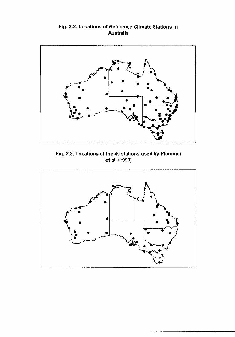
Fig. 2.2. Locations of Reference Climate Stations in Australia
• • •
.\P
Fig. 2.3. Locations of the 40 stations used by Plummer et al. (1999)
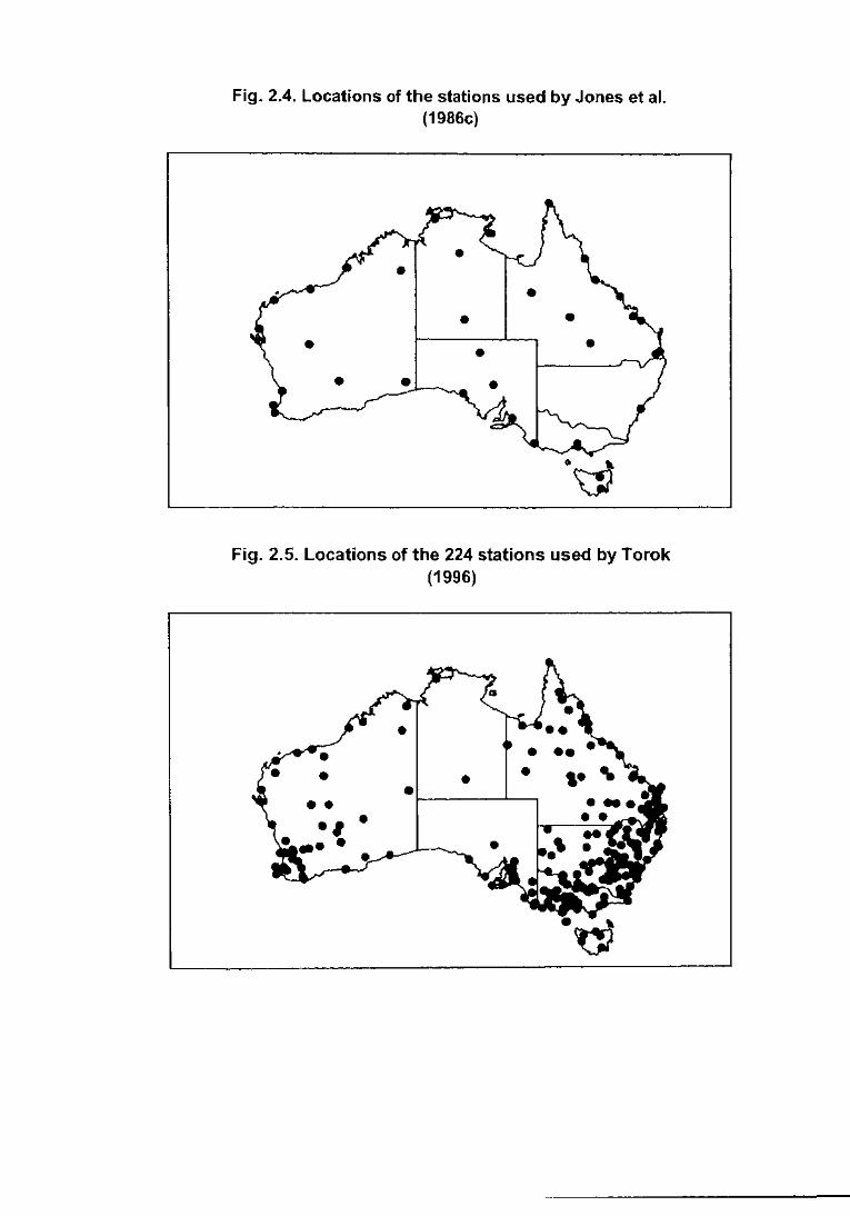
Fig. 2.4. Locations of the stations used by Jones et al. (1986c)
Fig. 2.5. Locations of the 224 stations used by Torok (1996)
•
• • ..,__ ___ ...____,
.u'
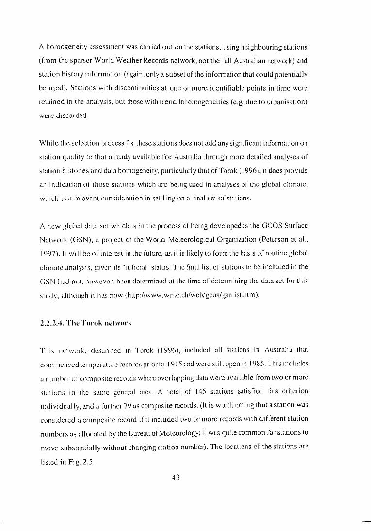
A homogeneity assessment was carried out on the stations, using neighbouring stations
(from the sparser World Weather Records network, not the full Australian network) and
station history information (again, only a subset of the information that could potentially
be used). Stations with discontinuities at one or more identifiable points in time were
retained in the analysis, but those with trend inhomogeneities (e.g. due to urbanisation)
were discarded.
While the selection process for these stations does not add any significant information on
station quality to that already available for Australia through more detailed analyses of
station histories and data homogeneity, particularly that of Torok (1996), it does provide
an indication of those stations which arc being used in analyses of the global climate,
which is a relevant consideration in settling on a final set of stations.
A new global data set which is in the process of being developed is the GCOS Surface
Network (GSN), a project of the World Meteorological Organization (Peterson et al.,
1997). It wi II be of interest in the future, as it is likely to form the basis of routine global
climate analysis, given its 'official' status. The final list of stations to be included in the
GSN had not, however, been determined at the time of determining the data set for this
study, although it has now (http://www. wn1o.ch/web/gcos/ gsnli st.httn).
2.2.2.4. The Torok network
This network, described in 'T'orok (1996), included all stations 111 Australia that
commenced temperature records prior to I 915 and were sti II open in 1985. This includes
a number or composite records where overlapping data were available from two or more
stations in the san1e general area. A total of 145 stations satisfied this criterion
individually, and a further 79 as cmnpositc records. (It is worth noting that a station was
considered a composite record if it included two or more records with different station
numbers as allocated by the Bureau of Meteorology; it was quite common for stations to
n1ove substantially without changing station number). The locations of the stations are
listed in Fig. 2.5.
43

All stations meeting the data availability criterion were included in Torok's analysis,
because of a lack of high-quality data. He did, however, rate all his stations on a scale of
1 to 5, based on a subjective assessment of the state of the site, the diligence of the
observers and the number of changes that had occurred through the record. The rating
applies to the entire period of the record; there are some stations which rate poorly over
the record as a whole but are good for some parts of the record.
In the context of this study, the main purpose of the Torok network is to provide an
indication of station quality (through the subjective ratings) and which stations have long
tenn records. While the existence of long-term records is not critical for this study, in
which the major constraint on the period of record used is the availability of daily digital
data rather than the overall length of record, if a station does have long-term data and is
included in the network, it allows this study to be extended backwards in time without
changing the station network should older daily data become available at some time in the
future.
2.3. The choice of a station network for this study
The Reference Climate Station network was used as the initial basis for the station
network in this study. This provides a good initial set of stations, to which modifications
can be made as necessary. While it would have been possible to include all Reference
Climate Stations, it was considered appropriate to exclude some from the data set, on the
grounds that they had insufficient data, poor recent data or duplicated other stations in the
RCS network.
The principal critetia used in selecting stations were the length of daily digital data
available (with 20 years being an absolute minimum), the quality of the data (either as
determined byPlummerand/orTorok, or by a station's standing as aRCS), and achieving
the broadest possible geographical coverage. The length of monthly data available was a
secondary consideration.
44
•

A total of 16 Reference Climate Stations were not included in this study. Four (Gove,
Tindal, Cape Grim and Liawenee) were excluded because they did not have 20 or more
years of data avai I able, two (Rottnest Island and Liverpool) because of substantial
missing data in the last few years, and one (Mount Isa) because of a major station move
towards the end of the record. The other nine stations were discarded because they were
considered to be sufficiently close in distance and similar in climate to other sites in the
network to be surplus to requirements. Of these nine stations, seven were not in either the
PI ummer or Jones net work (the exceptions being Gladstone, which duplicated Bundaberg
and Rockhampton as central Queensland coastal stations, and Cape Nelson, which
duplicated Cape Otway as a western Victorian coastal station and was also close to,
although somewhat n1ore exposed than, Mount Gan1bicr), and three had digital daily data
cotnincncing in 1964 or later.
Thursday Island was included, even though it is now closed, as it only closed in 1995 and
no other record of any length exists from the Tones Strait islands. It may, in the future, be
possible to continue the record using data rrom Horn Island, 10 kilometres away.
Twcnty-fi vc stations were then added to the network. These were chosen on the following
has is:
Capital cities: The six state capital city sites were added to the network because of the
length or their records and the potential interest of the statistical nature of changes in their
c I i mate, e vcn i r they arc urbanisation-induced. These stations were excluded from certain
parts or the analysis where it was considered desirable to exclude data which might be
subject to an artificial warming trend.
Stations fro an the Plununcr/Joncs networks: Thirty stations were included in either the
Plumrncr or Jones networks which were not Reference Clin1ate Stations. (Fifteen of these
were in Queensland). These stations were examined to determine whether they would add
useful information to the network, by substantially improving its geographical coverage,
sampling a cliinatic type which was underrepresented in the Reference Climate Station
network, or inc] uding a station identified by Torok as having a long, high-quality record.
15 stations were added on this basis. Barcaldine was also added, despite its apparent
45
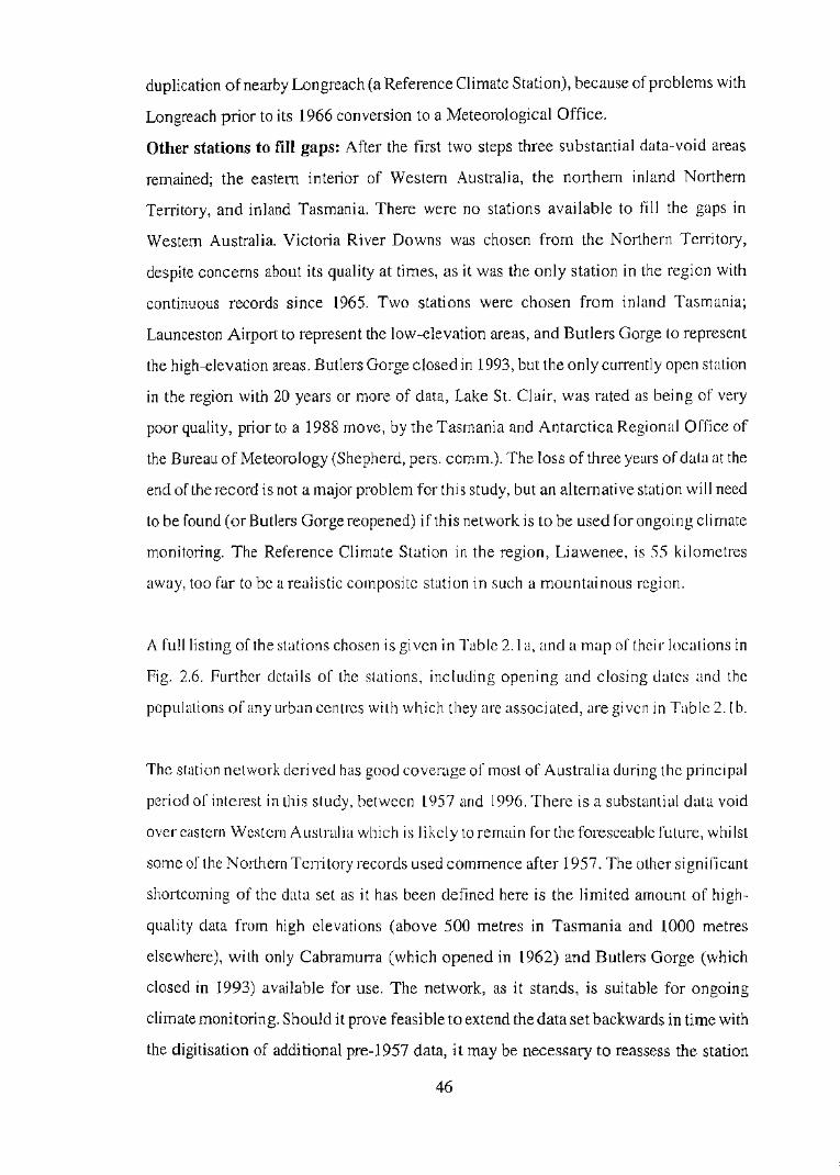
duplication of nearby Longreach (a Reference Climate Station), because of problems with
Longreach prior to its 1966 conversion to a Meteorological Office.
Other stations to fill gaps: After the first two steps three substantial data-void areas
remained; the eastern interior of Western Australia, the northern inland Northern
Territory, and inland Tasmania. There were no stations available to fill the gaps in
Western Australia. Victoria River Downs was chosen from the Northern Territory,
despite concerns about its quality at times, as it was the only station in the region with
continuous records since 1965. Two stations were chosen from inland Tasmania;
Launceston Airport to represent the low-elevation areas, and Butlers Gorge to represent
the high-elevation areas. Butlers Gorge closed in 1993, but the only currently open station
in the region with 20 years or more of data, Lake St. Clair, was rated as being of very
poor quality, prior to a 1988 move, by the Tasmania and Antarctica Regional Office of
the Bureau of Meteorology (Shepherd, pers. comm.). The loss of three years of data at the
end of the record is not a major problem for this study, but an alternative station will need
to be found (or Butlers Gorge reopened) if this network is to be used for ongoing climate
monitoring. The Reference Climate Station in the region, Liawenee, is 55 kilometres
away, too far to be a realistic composite station in such a mountainous region.
A full listing of the stations chosen is given in Table 2.1 a, and a map of their locations in
Fig. 2.6. Further details of the stations, including opening and closing dates and the
populations of any urban centres with which they are associated, are given in Table 2. I b.
The station network derived has good coverage of most of Australia during the principal
period of interest in this study, between 1957 and 1996. There is a substantial data void
over eastern Western Australia which is likely to remain for the foreseeable future, whilst
some of the Northern TeiTitory records used commence after 1957. The other significant
shortcoming of the data set as it has been defined here is the limited amount of high
quality data from high elevations (above 500 metres in Tasmania and 1000 metres
elsewhere), with only Cabramurra (which opened in 1962) and Butlers Gorge (which
closed in 1993) available for use. The network, as it stands, is suitable for ongoing
climate monitoring. Should it prove feasible to extend the data set backwards in time with
the digitisation of additional pre-1957 data, it may be necessary to reassess the station
46
..
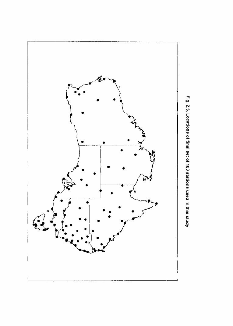
., ((l'
1\)
!'> r-0 0 D)
~ 0 ::::l tJ)
0 .... ::!1 ::::l e!. tJ) Cb ..... 0 .... ...,A.
0 (,J
tJ) -Q) -c;· :J tJ)
c tJ) Cb 0.
:J -0
d ~
iii' flj ..... c 0. '<

Station Station name Latitude Longitude Altitude Station Station number (deg S) (deg E) (m) category networks
1021 Kalumburu 14.17 126.38 23 R R 2012 Halls Creek AMO 18.14 127.40 422 A (ST) R, J, P, T* 3003 Broome AMO 17.56 122.14 7 A (LT) R, J, P, T* 4032 Port Hedlund AMO 20.22 118.38 9 A (LT) R, J, P, T* 5007 Lcarmonth AMO 22.14 114.05 5 R R 5026 Wittcnoom PO 22.14 118.20 463 R R,P 6011 Carnarvon AMO 24.53 113.40 4 A (ST) R,J, T* 7045 Meckatharra AMO 26.37 118.32 517 A (ST) R, J, P, T* 8039 Dalwallinu PO 30.17 116.40 335 R R,P 8051 Gcraldton AMO 28.47 114.41 33 A (LT) R,P 9021 Perth Airport 31.5() 115.56 20 A (U) <)518 Cape Lecuwin 34.22 115.08 14 R R,1, T 9500 Albany Town 35.01 117.52 18 LT R,T* 9741 Albany AMO 34.56 117.48 68 A (LT) R,T* 9541 Esperance PO 33.51 121.53 4 ST R,P,T* <J78'J Esperance MO 33.50 121.53 25 A (ST) R,P,T* 10035 Cunderdin PO 31.39 117.14 236 R R,P 10()48 Wandering 32.40 116.40 280 R R,P,T 1 1004 r;·orrest AMO 30.50 128.07 156 R R, 1, p 11052 Forrest A WS 30.50 128.07 156 R R,1, p 12038 Kalgoorlie AMO 30.47 121.27 365 A (LT) R, 1, P, T* 1]017 Giles MO 25.02 128.17 598 R R,P 14015 Darwin Airport 12.25 130.53 31 A (LT) R,1, T* 14825 Victoria River Downs 16.24 131.01 82 R 15087 Tennant Creek PO 19.37 134.11 377 ST R 15135 Tennant Creek MO 19.38 134.11 375 A CST) R 15548 Rabbit I :I at 20.11 130.01 340 R R 155<)0 Alice Springs MO 23.48 133.53 546 A (LT) R, 1, T* 1(>001 Woomera AMO 31.08 136.4') 165 A CST) R, 1, p 1(>044 Tarclll >Ia 30.42 134.35 1 19 R R I C>O<J8 Tarwola (new site) 30.42 134.35 12.3 R R 170.11 MarTt.:e PO 2<)J<) 138.03 50 R R 170·U ( )odnadatla !\ WS 27.34 135.26 113 R 1
( l'ormt.:rly MO) 1711--1- ( )odnadatta PS 27J2 135.2() 120 R 1 IXOI2 ('cduna AMO 32.0X 133.42 15 A (ST) R, 1 18070 Purl l.incoln PO 34.43 135.51 4 LT T 2 I 0--1-<> Snowtown PO 33.47 138.13 10.3 R R,T :2:2801 ('apt: Borda 35.45 136.35 143 R R,T :2.1000 Adelaide (W.Terrace) 34.56 138.35 40 u 1, T* :2J()l)() Adelaide (Kent Town) 34.55 138.37 48 u 1, T*
:2.1321 Nurioolpa 34.28 139.00 274 A(ST) R,P 23.173 N mioolpa A WS 34.29 139.00 275 A (ST) R,P 2(>0:21 Mount Gambier AMO 37.44 140.47 ()3 A (LT) R, 1, T* 2(>0:26 Rube PO 37.10 139.45 3 R R,T :27022 Thursday Island MO 10.35 142.13 58 A (ST) R,J,P, T* 27042 Weipa Composite 12.37 141.53 11 ST R 27045 Weipa MO 12.40 141.55 20 A (ST) R
28004 Palmcrvillc 16.59 144.04 204 R P,T
29004 Burkctown PO 17.44 139.32 5 R R,P,T ]0045 Richmond (Qld.) PO 20.44 143.08 211 R R,T
31011 Cairns AMO 16.53 145.45 3 A (LT) R, J, T*
Table 2.1a. Final list of stations used in this study
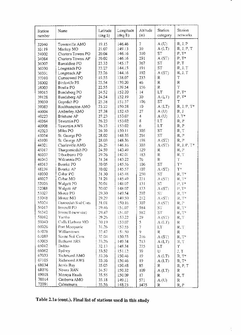
Station Name Latitude Longitude Altitude Station Station
number (deg S) (deg E) (m) category networks
32040 Townsville AMO 19.15 146.46 7 A (U) R,.J,P
33119 Mackay MO 21.07 149.13 30 A (LT) R,.J,P,T
34002 Charters Towers PO 20.04 146.16 310 ST P,T*
34084 Charters Towers AP 20.02 146.16 291 A (ST) P,T*
36007 Barcaldine PO 23.33 145.17 267 ST P,T
36030 Longreach PO 23.27 144.15 191 ST R, J, T
36031 Longreach AP 23.26 144.16 192 A (ST) R,.J,T
37010 Camooweal PO 19.55 138.07 233 R T
38002 B irdsville PS 25.54 139.20 46 R R
38003 Boulia PO 22.55 139.54 156 R T
39015 B undaberg PO 24.52 152.20 14 LT P,T*
39128 B undaberg AP 24.54 152.19 30 A (LT) P,T*
39039 Gayndah PO 25.38 151.37 106 ST T
39083 Rockhampton AM 0 23.22 150.28 10 A (LT) R, .I,P, T*
40004 Amberley AMO 27.38 152.43 27 A (U) R, J 40223 Brisbane AP 27.23 153.07 4 A (U) J, T* 40264 Tewantin PO 26.23 153.02 8 LT R, p
40908 Tewantin A WS 26.23 153.02 6 LT R, p
42023 Miles PO 26.39 150.11 305 ST R,T 43034 St. George PO 28.02 148.35 201 ST R, p
43109 St. George AP 28.03 148.36 198 A (ST) R, P 44021 Charleville AMO 26.25 146.16 303 A (ST) R,.l, P, T* 45017 Thargomindah PO 24.59 143.49 129 R R, p
46037 Tibooburra PO 29.26 142.01 183 R R,T 46043 Wilcannia PO 31.34 143.22 76 R T 48013 Bourke PO 30.05 145.56 106 ST T* 48239 Bourke AP 30.02 145.57 107 A (ST) T* 48030 Cobar PO 31.30 145.48 250 ST R,T* 48027 Cobar MO 31.29 145.49 221 A (ST) R,T* 52026 Walgett PO 30.01 148.07 131 ST P,T* 52088 Walgett AP 30.02 148.07 133 A (ST) P,T* 53027 Moree PO 29.30 149.54 207 ST R,T* 53048 Moree MO 29.29 149.50 212 A(ST) R,T* 55024 CJunncdah Soil Cons 31.0 I 150.16 307 A(ST) R, p 56017 Invcrcll PO 29.46 15 1.07 584 ST R,T* 56242 Invcrell (new site) 29.47 I 5 1.07 582 ST R,T* 58012 Yi.unba 29.26 153.22 29 A (ST) R,T 59040 ColTs 1Iarbour MO 30.19 153.07 5 A (LT) R 60026 Port Macquarie 31.26 152.55 7 LT R,T 61078 Williamtown 32.47 151.50 9 R R 61089 Scone Soil Cons 32.04 150.55 216 A (ST) R,T* 63005 Bathurst ARS 33.26 149.34 713 A (LT) R,T 65012 Dubbo 32.13 148.34 275 LT T 66062 Sydney 33.52 151.12 39 u J, T 67033 Richmond AMO 33.36 150.46 19 A (LT) R,T* 67105 Richmond A WS 33.36 150.46 19 A(LT) R,T* 68034 Jervis Bay 35.05 150.48 85 R R,P, T 68076 Nowra RAN 34.57 150.32 109 A(LT) R 69018 Moruya Heads 35.55 150.09 17 R R,T 70014 Canberra AMO 35.18 149.11 571 A(U) R 72091 Cabramurra 35.56 148.23 1475 R R,P
Table 2.1a (cont.). Final list of stations used in this study

Station Name Latitude Longitude Altitude Station Station number (deg S) (deg E) (m) category networks
72150 Wagga Wagga AMO 35.10 147.27 212 A(LT) R,T* 73054 Wyalong PO 33.55 147.14 245 R R 74128 Deniliquin PO 35.33 144.56 93 ST R,T 76031 Mildura AMO 34.14 142.05 51 A(LT) R,T* 78031 Nhill 36.20 141.38 133 ST R,P,T 80023 Kcrang PO 35.44 143.55 78 ST P,T 82039 Rutherglcn Rc1-learch 36.06 146.30 168 A (ST) P, T* 8401() Gabo Island 37.34 149.55 15 R T 84030 Orbost 37.41 148.27 41 ST R 85072 East Sale AMO 38.06 147.08 5 A(LT) R,T* 8509() Wi !sons Promontory 39.08 146.25 89 R R, J, T 86071 Melbourne 37.48 144.58 35 u J, T 87031 Lavcrton AMO 37.52 144.44 18 A(U) R,T* 90015 Cape Otway 38.51 143.31 82 R R,P,T 91057 Low I lead 41.03 14(>.47 28 R R,T 91104 Launceston AP 41.34 147.12 170 A (LT) J, T* l)2045 Eddystone Point 40.59 148.20 13 R R 94010 Cape Bruny 43.29 147.08 55 R R 94198 Cape Bruny AWS 43.29 147.08 60 R R 94029 I lob art 42.53 147.19 55 u J, T 940Cl9 (]rove Research 42.59 147.04 60 R R,P 9()()()3 Butlers Gorge 42.16 146.16 ()(16 R
Table 2.1 a (cont.). Final list of stations used in this study
Explanation of syrnhols used in table
Sym hoi I~xplanati<Jn
Site /\MO Airport M!.!teorological Office MO Metl!orological Office PO Post Office J>S Police Station AP Airpmt /\WS Automatic Weather Station /\RS Agricultural Research Station
Station ]{ I< ural site or in settlement with population less than 1,000 location ST Small town (population I ,000 - 1 0,000)
LT Large town (population 10,000 - 1 00,000) u Major urban centre (population greater than 1 00,000) A(ST) Airport or similar site (e.g. research farm) in vicinity of population centre. Symbol in
parentheses indicates size of associated population centre. Airports not associated with a population centre> 1,000 (e.g. Porrest, Lcannonth) arc shown R. All populations are as of the 1996 Census.
Station R Reference Climate Station networks .J Slation net work used by Jones et al. (1986c)
p Station network used by Plummer et al. ( 1999) ·r Stntion with long record as identified by Torok (1996) (*-as composite)

Station Station name Year First Year Population of associated centre (Census) number open digital closed
data 1954 1976 1996
1021 Kalumburu 1942 1957 2012 Halls Creek AMO* 1944 1944 370 767 1263 3003 Broome AMO* 1939 1939 1093 2920 11368 4032 Port Heclland AMO* 1948 1948 895 11144 12846 5007 Lcarmonth AMO 1975 1975 5026 Wittenoom PO 1952 1958 962 6011 Carnarvon AMO* 1945 1945 1453 5341 6357 7045 Meckatharra AMO* 1950 1950 1100 829 1270 8039 Dalwallinu PO 1956 1957 683 697 8051 Gcralclton AMO* 1941 1941 8308 18773 25243 9021 Perth Airport 1944 1944 348596 731275 109(J829 9518 Cape Lecuwin 1897 1957 9500 Albany Town 1880 1950+ 1965 82(>5 13696 20493 9741 Albany AMO 19(J5 1965 82(>5 1369() 20493 9541 Esperance PO 1883 1957 1969 1087 5262 8647 9789 Esperance M 0 1969 1969 1087 5262 8647 10035 Cundcrdin PO 1950 1957 756 715 1064~ Wandering 1902 1957 11004 F()rrcst AMO 1946 194(> 1995 11052 I ;l >rrcst 1\ WS 1993 1993 12038 Kalgomlic AMO* 1939 1939 22834 19041 28087 13017 Ciiles MO 195(1 1956 14015 Darwin Airport* 1941 1941 8071 41374 70251 14825 Victoria River Downs 19(J5 19(>5 15087 Tennant Creek PO I 92(> 1957 1970 959 2236 385() 151}5 Tennant Creek MO 1969 1969 959 2236 3856 155·HI Rabbit 1 :I at 10(>9 19(>9 15590 Alice Springs MO* 1941 1941 2785 14149 22488 I (>00 I Woomcra AMO 1949 1949 2958 1349 I (>044 TarnH>Ia 1022 J 950+ 1997 I (>09S Tarcuo1a (new site) 19l)7 1997 170.11 Marrec J>() 1939 1957 334 17043 Oodnadatta A WS 1940 1940 229
( l'ormcr1y MO J
17114 C h >dnadatta PS 19H5 1985 1991 229 ISOI2 < 'eduna AM()'+' 1939 1939 1953 2327 2599 Jr:070 Port Lincoln J>() 1022 1957 5871 10272 J 1678 2 I 04(> S!l()WtDwn )>() 1925 1957 511 429 22r:01 ('ape Borda 1025 1957 23000 Addaide ( W. Terrace) 1887 1RH7 1979 483535 H57196 978100 23090 Ad~laidc (Kent T()WJl) 1977 1977 483535 857196 978100 23321 Nuriuotpa 1952 1957 1465 2808 3486 23.17.1 Nuriootpa A WS 1996 1996 1465 2808 3486 2C>021 Mt Gambier 1\.MO* 1942 1942 10334 19292 22037 2C>02C> Robe PO 1957 1957 490 816 27022 Thursday Island MO* 1950 1950 1993 27042 Weipa composite 1959 1959 1994 2876 2200 27045 Weipa MO 1992 1992 2876 2200 28004 Palmervi1le 1907 1957 29004 Burkctown PO 1907 1957 220
30045 Richmond (Qld.) PO 1908 1957 881 733
31011 Cairns AMO* 1942 1942 21021 39305 92273
Table 2.lb. Stations used in study· opening and closing dates, city populations

Station Station name Year First Year Population of associated centre (Census)
number open digital closed data 1954 1976 1996
32040 Townsville AMO* 1940 1940 40485 78653 109914
33119 Mackay MO* 1959 1959 14764 31522 44880
34002 Charters Towers PO 1907 1957 1992 6960 7914 8893
34084 Charters Towers AP 1992 1992 6960 7914 8893
36007 Barcaldine PO 1913 1957+ 1705 1443 1592
36030 Longreach PO 1907 1957 1973 3356 3354 3766
36031 Longreach AP 1966 1966 3356 3354 3766
37010 Camooweal PO 1907 1957 1997 322 258
38002 Birdsville PS 1954 1957
38003 Boulia PO 1888 1949+ 272 243
39015 Bundaberg PO 1907 1957 1990 19953 31189 41025
39128 Bundaberg AP 1959 1959x 19953 31189 41025
39039 Gayndah PO 1894 1957 1644 1643 1781
39083 Rockhampton AMO* 1939 1939 40676 50132 57770
40004 Amberley AMO 1941 1941 502353 892987 1291117
40223 Brisbane AP 1949 1949 502353 892987 12<)1117
40264 Tewantin PO 1949 1957+ 1996 1766 5834 2(J053**
40908 Tewantin A WS 1996 1996 1766 5834 2()()53**
42023 Miles PO 1908 1957 1193 1367 1187
43034 St. George PO 1938 1957+ 1997 1698 2095 24(J]
43109 St. George AP 1997 1997 1698 2095 24(13
44021 Charleville AMO* 1942 1942 4517 3802 3327 45017 Thargomindah PO 1938 1957 21.')
46037 Tibooburra PO 1910 1921+ 211 46043 Wilcannia PO 1881 1957 1023 48013 Bourke PO 1871 1957 199(J 2642 3534 2775 48239 Bourke AP 1994 1994 2642 3534 2775 48030 Cobar PO 1890 1957 1965 2223 3339 4524 48027 CobarMO 1962 1962 2223 3339 4524 52026 Walgett PO 1878 1957 1993 1348 2253 j<J7()
52088 Walgett AP 1993 1993 1348 2253 j<J7()
53027 Moree PO 1879 1879+ 1966 5501 <)].)<) <J270 53048 Moree MO 19(14 19(14 5501 935<) <)270
55024 Gunncdah Soi I Cons* 1948 1959+ 5129 8(J8<) t1315 56017 lnverc11 PO 1907 1957 1997 7517 9432 CJ37X 56242 1nverc11 (new site) 1995 1995 7517 9432 937t1 58012 Yamba 1877 1921+ 1649 4721 59040 Coils Harbour MO* 1943 1943 (J214 12197 22177 60026 Port Maequarie 1907 1921+ 4423 13362 33709 61078 Wi11iamtown 1942 1942 61089 Scone Soil Cons* 1952 1959+ 3351 3424 34M; 63005 Bathurst ARS* 1909 1909+ 16090 18589 2(J029 65012 Dubbo 1871 1957 12025 20149 30102 66062 Sydney 1859 1859 1863217 2765040 3276207 67033 Richmond AM 0* 1939 1939 1994 9867 13340 21317 67105 Richmond AWS 1994 1994 9867 13340 21317 68034 Jervis Bay 1907 1921+ 68076 Nowra 1955 1955 5981 15496 23823 69018 Moruya Heads 1876 1921+ 70014 Canberra AMO* 1939 1939 35584# 213055# 324932# 72091 Cabramurra 1962 1962 203 72150 Wagga Wagga AMO* 1942 1942 19243 32984 42848 73054 Wyalong PO 1950 1959+ 74128 Deniliquin PO 1858 1949+ 4705 6865 7816
Table 2.1b (cont.). Stations used in study · opening and closing dates, city populations

Station Station name Year First Year Population of associated centre (Census) number open digital closed
data 1954 1976 1996
76031 Mildura AMO* 1946 1946 10971 14417 24142 78031 Nhill 1897 1951 2208 2124 1890 80023 Kerang PO 1903 1957+ 3326 4022 3883 82039 Ruthcrglen Research 1913 1957+ 1912 1325 1904 8401() Gabo Island 1877 1957 84030 Orbost 1938 1957 2215 2789 2150 85072 East Sale AMO* 1945 1945 6536 12111 13366 85096 Wilsons Promontory 1877 1890+ 86071 Mclh<)urnc 1855 1855 1524062 2479225 2865329 87031 Laverton AMO* 1943 1943 1524062 2479225 2865329 90015 Cape Otway 1865 1957 91057 Low I lead 1895 1957 91104 Launceston AP 1939 1939 49310 63386 67701 92045 Eddystone Point 1957 1957 94010 Cape Bruny 1924 1957 94198 Cape Bruny A WS 1997 1997 94029 I lobart 1881 1944 95223 131524 126118 94069 Grove Research 1952 1957 9()()()3 Butlers Clorge 1944 1957 1993
'fable 2.1 h (cont.). Stations used in study· opening and closing dates, city populations
Symbols us<.:d in the table:
* Another station in the area (usually without digital daily recorus) exists and c..:ould potentially be used as a cumposite to extend the data back in time.
+ Includes thtla digitised manually as part or this and other projects that is not available through regular Bureau channels.
x Bunda berg Airporl has data for I 959-71 and 1990 onwards. The 1959-71 data is u:-;ed for comparison purposes llnly.
** ( 't1mhined population of Tewantin-Noosa. # ( 'tHnhined populatitm of' Canberra-Qucanheyan.
Dates gJVL'll under 'year open' are the earliest year for which monthly temperature data is available in the Bureau digital arc hi vcs. Some data exists from prim to this date at a number or stations (notably Robe). There are breaks in the data at stHllc statitlllS. All stations without a closure elate listed arc currently open.

network (possibly using additional stations with data from 1908 or earlier to supplement
the numerous Meteorological Office sites that opened between 1939 and 1950), and the
coverage of central Australia will be more limited than it is with the present network.
47

Chapter 3
Some systematic issues influencing quality of daily
temperature data in Australia
3.1. Introduction
Climate data arc subject to numerous systematic inhomogeneities. These
inhomogeneities, which arc elaborated on in Chapter 4, include station moves,
instrurncnt changes, changes in site condition and local land use and changes in
ohservation practices. A crucial aspect or the development of any high-quality
ternperaturc data set is the manner in which data are adjusted to remove these
inhon1ogcncitics frorn the climate record. This is a particular challenge in the case of
daily data. A new technique for the adjustment of daily data is presented in section
3.2.
Two issues which have the potential to affect temperature records in a systematic
manner arc changes in the time of observation, and the use of accumulated data after a
missed observation. These arc discussed in sections 3.3 and 3.4 respectively.
3.2. Methods of producing con1posite daily tentpcrature data sets from
inhornogcncous data
Standard procedures for adjustments of mean temperatures in order to remove non
climatic inhomogeneities have relied on the implicit assun1ption that, if two
neighbouring stations have homogeneous records over some period of tirne, the
dillcrcnce in daily n1aximun1 (or minimmn) temperature between thcn1 will be a
constant for any clay in a given 1nonth of the year. This implies that the difference in
monthly n1cans wi II be constant for that month fron1 year to year. This assumption is
inherent in works such as Barger and Nyhan (1960), Karl and Williams (1987), Torok
(1996), Torok and Nicholls (1996), and has been built into software systems such as
the THOMAS systen1 used in Slovakia and Switzerland (Begert et al., 1998) and the
MASH system developed in Hungary (Szentimrey, 1998), which has been widely 49
used in the development of indices of extreme climate events (e.g. Manton et al.,
2001). In one of the few attempts to produce homogenised series of extreme event
frequencies, in Austria (Auer et al., 1998), uniform monthly adjustments were applied
to daily data. It appears to originate from work by Mitchell (1961 ), who established
that there was no relationship between the difference in mean monthly temperature for
February between two sites at Blue Hill, Massachusetts (one on the summit, one at the
base) and the actual temperature at one of the sites. Since that time, refinements of
methods for removing inhomogeneities (e.g. Karl and Williams, 1987) have
concentrated on the accurate determination of the point in a record at which an
inhomogeneity exists, and the selection of the most appropriate neighbouring
station(s) for use in adjustment.
A different approach was adopted in a very recent paper by Allen and DeGaetano
(2000), who were investigating inhomogeneities in time series of the number of days
per year above or below given thresholds. They initially used metadata to identify
potential inhomogeneities (although they note that the use of metadata is not
fundamental to their technique, and that statistical techniques could be used instead),
compiled a difference series involving the 25111 and 75 111 percentiles of the number of
days per year above/below their chosen threshold at the candidate station and a
weighted sum of neighbouring stations, and tested for changes in those difference
series. They then 'adjusted' the time series by an iterative process involving the
changing of their thresholds on one side of the identified inhomogeneity, until no
significant change in the adjusted difference series could be identified.
It is, however, well documented that local influences on climate, such as the intensity
of urban heat islands (Bernhofer, 1984; MoiTis and Simmonds, 2000; Mon·is et al.,
2001) and the influence of cold-air drainage (Kalma et al, 1992) are not constants, but
are dependent on factors such as wind speed and direction and cloud amount. At a site
such as Blue Hill in winter, where the dominant influence on temperature is non
periodic air mass advection, these are not major factors and the assumption that
temperature is independent of, say, wind speed is not unrealistic. This results in any
discrepancies in the temperature differences being distributed randomly in the record
and not creating a bias. However, at many sites, and in particular, in much of inland
50

Australia, the dominant influence on minimum temperatures is radiational cooling and
thus there will be a tendency for light winds to be associated with low temperatures
(Kalma et al, 1992). This is observed at Armidale (Burr, pers. comm.), one of the sites
considered further in this section, where the difference in minimum temperature
between the town centre site used in this study and a second site approximately 2 km
to the east (which has been the Bureau of Meteorology's official site in Armidale
since June 1997 but has been operating unofficially since 1981 ), in the outer patt of
the town, has a mean value of 1.5 to 2°C, but can increase to 4°C on cold, clear
nights. Thompson ( 1973b) also found that the temperature difference between a
hilltop and valley site in the Armidalc area varied depending on the circulation type
over the region. It is also known (e.g. Gall et al., 1992) that the difference in
temperature bet ween a poorly-ventilated i nstrumcnt and a well-ventilated one wi 11
reach its maximum under sunny conditions in sun1mer, suggesting that the
ternperature difference between them would increase with increasing temperature.
The assun1ption that the temperature difference between any two nearby sites is
always constant must therefore be questioned.
This section proposes alternative methods for constructing composite daily
temperature records where that assumption breaks down, using four station pairs in
south-eastern Australia. While this is only a small part of the globe, the results
obtained arc potentially or wide general applicability.
3.2.1. Methods and station selection
Fig. ].1 shows the location of the stations used in this section, with Table 3.1 giving
Jctai Is ol' the sites. Station pairs were selected with the intention of illustrating the
varying influences on temperature at contrasting sites. The do1ninant contrast at these
sites is topography and exposure. While, ideally, a pair would have been investigated
in order to show the effect of an urban and non-urban site, to achieve this it would be
necessary to choose an urban centre in a flat region (to remove any effects of
topography) away from the coast (to remove the influence of exposure to the ocean).
There are few centres of this type in Australia with populations in excess of 10,000,
and none of those that exist (e.g. Dubbo, Wagga Wagga) have a pair of stations, one
51

urban and the other non-urban, with a reasonable period of overlap. Stanthorpe and
Tenterfield, a pair of sites with very similar characteristics, may be regarded as a
'control' pair which illustrates conditions at stations which do not show significant
contrast. (This is important in the development of methods for the adjustment of data,
as such methods must perform well in the case of all discontinuities of a record, not
just those which involve a major change in topography and/or exposure). The choice
of station pairs within south-eastern Australia was constrained primarily by the
limited number of neighbouring sites available with a reasonable length of
overlapping record. Those pairs chosen had an overlapping record of between 13 and
28 years.
The relationship between the temperature characteristics of the two sites in each pair
was examined, with the aim of determining an appropriate method for use in
extrapolating records at one site to records at the other. This is quite a common
situation if an attempt is being made to ensure records at an old site are consistent
with those at a new site (or vice versa), because a relationship between temperatures
at two sites during a period of overlap can be used to estimate temperatures at one site
from records taken at the other during periods when records are only available from
one site. This can also be (and is in Chapter 4) extended to the comparison of records
from two sites with little or no overlap with those at a third site as a method of
constructing a composite record for the pair. Ideally, to optimise the accuracy of such
a comparison, the period of common record should be as long as possible, providing
the records of the two sites are each reasonably homogeneous during that period. In
practice, the period or overlapping record associated with a station move is usually
much less than 13 years, but the conclusions drawn should sti II be applicable to
shorter records, albeit with a higher level of uncertainty.
For the duration of common record for each station pair, values were obtained at each
site (subject to the conditions below) for:
(i) all daily maxima or minima for a given month of the year;
(ii) monthly mean maxima or minima for a given month for each year;
(iii) annual mean maxima or minima for each year.
52

Fig. 3.1. Location of stations used for development of methods used for construction of composite records
KiandraJCa bramurra
•

Station name Latitude Longitude Altitude Years of Distance Location and exposure ('JS) rT~) (m) common between record sites
(krn)
lnvcrell PO 2(J.7H 151.11 603.5 28 2 Vacant lot on valley floor in town centre 1nvcrdl S<' 29.7H 151.08 707.1 On ridge on western edge of town
Kiandra l\HH 148.50 1395.4 13 12 On slope just above valley floor, on east side of range ( 'ahrarnurra 35.<):1 l48J8 1475.0 Near top of west-facing scarp. Very exposed to prevailing westerly winds
Armidak J0.52 15 1.65 979.9 23 56 Town centre; buildings and car parks nearby; on gentle slope
\V(H>IhnHlk 30.<)7 151J5 917.1 Valley floor in small village
StantiH >rpe 2H.(l5 151.93 792.2 28 44 Both sites on gentle slopes in Tcntcrfrcld :2().05 [ 52.02 862.6 town centres
Tahh.• J.l. Site details for station pairs used in section 3.2.

For simplicity, these are referred to henceforth as daily, monthly, and annual 'data
objects' respectively.
Days on which data were available for one site only were not considered for inclusion
in data objects (or the calculations of means) at the other. If fewer than 10 days in any
month had data available at both sites, the means for that month, and hence that year,
were regarded as missing.
If we consider two data objects for a pair stations of the form (x1, x2, ••. ) and (y 1, y2, ... ),
the ordered pairs (xJ, Y1 ), (x2, Y2), ... were plotted, and a linear regression equation:
y =a+ bx
was fitted to the data points, using standard least-squares techniques.
3.2.2. Relationships between ten1peratures at paired sites
In this section, the null hypothesis that there is no relationship between the
temperature uillerence between the paired sites and the tenlperature at one or those
sites is tcstcu. This is equivalent to stating that h= 1 in the regression equation above.
A relationship between the temperatures, rather than between the tc1npcrature
di llcrence bet ween the sites and the temperature at one sites, is used to avoid any bias
that could arise from the choice of one or other of the paired sites as the 'base' against
which the temperature diiTcrence between the sites is cornparcd. The tests of
significance used are also based on the relationship between the temperatures at the
paired sites.
Tables 3.2 and 3.3 indicate months in which b departs from 1 at given levels of
significance. The relationships shown for daily, monthly, and yearly data objects,
respectively, in these tables are further illustrated by Figs. 3.2 and 3.3. In order to
make departures from the assumption of a constant difference more visually apparent,
one of the axes in each of these graphs is the temperature difference between the two
53

sites rather than the temperature at the second site.
Table 3.2 shows a highly significant departure of the coefficient b from 1 for daily
minima in all months at three of the four station pairs: Inverell, Kiandra-Cabramun·a
and Armidale-Woolbrook. There is also a significant departure for daily maxima in
most autumn and winter months at each of these pairs except Kiandra-CabramutTa.
There is much less evidence of a relationship in either case at the 'control' pair of
Stan thorpe-Tenterfield.
Table 3.3 indicates that a significant departure also exists for monthly mean minima
in most months at three of the pairs: Inverell, Kiandra-Cabramurra and Armidale
Woolbrook. These are the three pairs where the sites contrast substantially in local
topography. Except at Armidale-Woolbrook, significant departures also exist for
annual mean minima.
3.2.3. Comparison of percentile points in overlapping temperature records
The use of regression relationships indicates the presence of a statistically significant
dependence of temperature difference between sites on the temperature at one site for
some of the station pairs used in this study. It does not necessarily follow from this
that the relationship is linear.
Fig. 3.4, showing the frequency distribution of July minimum temperatures at the two
Inverell sites, and Fig. 3.5, giving specific points in these frequency distributions,
illustrate possible non-linearities in such relationships. Assuming that there is no
systematic difference in rank order of temperature between the two sites, the expected
difference in temperature between the sites is approximately constant for the coldest
65 percent of nights; it is only in the upper 35 percent of the frequency distribution
that the difference decreases.
54

Month Station pair
Inverell K i andra -Cabramurra Stan thorpe-Tenterfield Armidale-Wool brook
Max. Min. Max. Min. Max. Min. Max. Min.
January 1 1 5 1 February 5 1 1 5 1 March 5 I 1 1 April 1 1 5 5 1 May I I I 1 1 1 June I 1 I 1 July 5 1 I 1 1 August 5 1 I 5 1 I September I I I October I I 5 I November I I 1 December I I I
Table 3.2. Statistical significance of departures front unity in the slope of the regression line relating data at each station pair; daily maximmn and ntinintunt ternperaturcs. • I' and 4 5' denote a departure front unity in the slope of the regression line, h, significant at the 1 per cent or 5 per cent levels respectively. A blank entry denotes no departure significant at the 5o/o level.

Month Station pair
Inverell Kiandra-Cabramurra Stan thorpe-Tenterfield Armidalc-Wool brook
Max. Min. Max. Min. Max. Min. Max. Min.
January 5 1 5 February l March l 5 5 April 5 5 May l l June 1 l 5 July l 1 August I 1 September 5 October November I December I I Annual I 1
Table 3.3. Statistical significance of departures fron1 unity in the slope of the regression line relating data at each station pair; ruonthly and annual mean 1naxinnun and mininnun tcn1pcratures. The usage of' 1' and '5' in the table is as for Table 3.2.
-
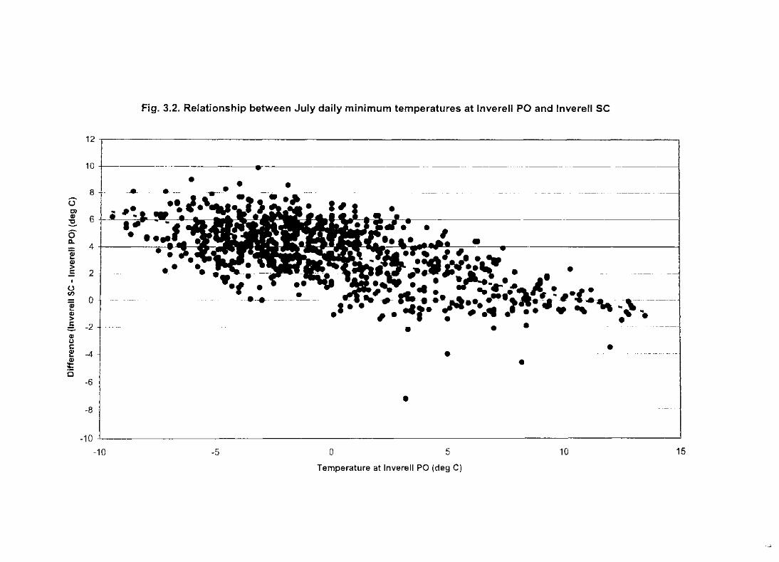
Fig. 3.2. Relationship between July daily minimum temperatures at lnverell PO and lnverell SC
12
10
8 - __ ,_._ ---~---- ---- --~-----~--~~--
u 0) CP 6 ~
0 D..
4 Qi ,_ C1l > -= 2 •
I
u en Qi 0 ,_ C1l > g -2
,. • •
-. C1l (.) c CP -4 ,_ • • £ • 0
-6
• -8
-10
-10 -5 0 5 10 15
Temperature at lnverell PO (deg C)
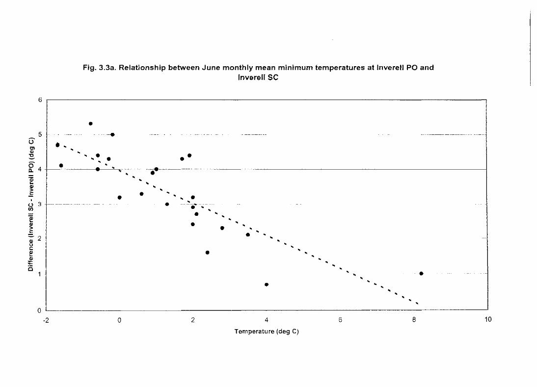
Fig. 3.3a. Relationship between June monthly mean minimum temperatures at lnverell PO and
lnverell SC
6 ~--------------------------------------------------------------------------------------------~
-5 -l~ (.)
Ol C1)
. ... ... "'C -~4 • -; ... ~ c
~ 3 -f--~--~~-----
-e Q)
> c :::.2 Q) (.) c ~ £ 0
0 -2
...
• •
... • • ... ... ... • ...
-- ... ... ... "
• •
0
• • ••
... ... ... ....... --- ---~----~ ...... --·;·-~-~-~ -
• ... ... ...
• •
•
2
... ... ... ... • ... .... ... ... ... ...
•
4
Temperature (deg C)
... ... ... ... ... ... ... ~ ·--~ ~~~~~---i " ... ... ... ... ... ... ... ... ...
6 8 10

Fig. 3.3b. Relationship between mean annual minima at lnverell PO and lnverell SC
4~------------------------------------------------------------------------------------------------~
3.5
6 C)
• IIIII .. • • Q)
~ .. ... .. ...
6 3 ll..
f C)
---
• ...
... - - - -- ... - .. -• ... ... ... fl' .. ..
> -= '
... .. .. • .. .. (.) 2.5 en
....... • • ... a; '""
.. • .. Q) > g Q) 2 -~------ --(,.)
• • .. ... • ... .. _,.,._-.. .. s::: ~ £
.. .. ... .. ... • .. • • c 1.5
6 6.5 7 7.5 8 8.5 9 9.5
Temperature at lnverell PO (deg C)
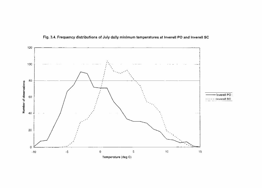
Fig. 3.4. Frequency distributions of July daily minimum temperatures at lnverell PO and lnverell SC
120~----------------------------------------------------------------------------~
' I '
100 r-- ___ -~"-- ----~--------<--
' , ' ... I ... ,
I
1\ I
I . 11) 80 s: 0 ;: ..., c:: Q) 11) .c ---lnverell PO 0 - - - - - - - lnverell SC 0 ... (1) .c E :s :z 40
20
0 . .. .
-10 -5 0 5 10 15
Temperature (deg C)

Fig. 3.5. Difference between percentile points of frequency distributions of July daily minimum
temperatures at lnverell PO and Soil Conservation Research Station
5 .---------------------------------------------------------------------------------------------~
4T-------------------------~--------------------------~---e~-----------------------------4
63 Ol G)
"'C -<U (.) s::: ~ ~ ·- 2 c
1 -
0 ~----------------------------------------------------------------------------------~ 0 10 20 30 40 50 60 70 80 90 100
Percentile 91
3.2.4. Possible techniques for the interpolation of temperature records
As a result of the relationships found above between temperatures at adjoining sites,
three techniques were considered for the interpolation of records. In each case, the full
period of available common record for a given station pair was used as a base for
calculating the parameters used in the interpolation, in which a synthetic series of
daily maxima and minima at one station was created using data from the other in the
patr.
(a) The 'traditional' constant-difference approach
The difference in maximum (or minimum) temperature between the sites on each day
was taken as the difference between the mean monthly maxima (or minitna) at the two
sites for the month concerned during the period of overlap.
(b) T'hc 'regression' n1ethod
'fhc coefficients and equation generated in section 3.2.1 were used to estimate
tcrnperaturcs at one site using those at the other.
(c) Frequency distribution matching
The 5 through to 95 percentile points (at 5 percentile intervals) for daily maxima and
minin1a for each month at each site, using data from the period of overlap, were
calculated. These points were denoted 'matching points'. To create a synthetic series,
the position of each day's temperature at the first site in the appropriate frequency
distribution was found, and the temperature difference between the sites estin1ated
using the formula:
55
T _ T, = T, . + (T2,(i+Sl - T2,i )(7; - ~.i) 2 1 1,1 (T, T, )
where T2
l,(i+5) - 1,i
denotes the estimated temperature at the second site
the actual temperature at the first site
the nearest matching point below T1 in the frequency
distribution of temperature at the first site (the i-th percentile)
T2,i the i-th percentile point in the frequency distribution at the second site
Where T1 is below the 5 percentile or above the 95 percentile level, the temperature
difference between the sites was taken as (T2,s- T1,5) or (T2,95- T1,95) respectively. An
alternative would be to use the highest or lowest temperature on record as matching
points, but this would be very sensitive to individual, and possibly enoneous, outlying
observations.
T2 was then found using the difference found above and the known value of T1.
3.2.5. An evaluation of the techniques for composite record developn1ent
A number of indicators were chosen to assess the accuracy with which the procedures
considered simulated the actual temperature record. These were chosen to reflect
possible features that may be of interest in the investigation of a temperature record:
the accuracy of the record as a whole, the frequency of temperatures above or below a
certain level (e.g. the frequency of frost), and the highest and lowest temperature in
the record.
Firstly, each of the three synthetic series was compared with the actual record for that
site, and a root-mean-square enor (Erms) calculated for each month, using:
56

Erms = i(T;-P;/
i=l n
where Ti represents the actual maximum or minimum temperature (or mean
maximum or minimum in the appropriate tables)
the modelled maximum or minimum temperature
n the number of observations considered.
Results of this procedure are given in Tables 3.4a, 3.4b and 3.4c.
Tables 3.5 and 3.6 show the estimated frequency and magnitude of extreme events
using the three procedures. The need for a separate consideration of extreme events is
illustrated by Fig. 3.5, which shows the non-linearity of the relationship between
winter minirnum temperatures at the two Invercll sites. This shows that, although
assuming a constant temperature difference will lead to an underestimate of the
temperature di rrerence on the coldest nights, attempting to represent the difference by
a linear relationship will lead to an overestimate of the difference. In the case of
lnvercll, 'T'ablc 3.5 shows that procedure B underestimates the frequency of minima
below ooc at the Soi I Conservation Research Station.
Tables 3.4a, 3.4b, 3.4c, 3.5 and 3.6 indicate that, for two of the site pairs (Stanthorpc
Tenterfieid and Annic.lalc-Woolbrook) the difference between the outcomes of
procedures A, I3 and C, regardless of the indicator of accuracy chosen, is minitnal.
These two pairs or sites arc those with the weakest relationships between temperature
dillerencc and temperature, as indicated by Tables 3.2 and 3.3. Where there is no
evidence or any relationship, as at Stanthorpe-Tenterfield, the results of the three
procedures converge, as expected. If there is no relationship at all, the slope of the
regression line in procedure B will be l.O and procedures A and B will therefore be
equivalent; similarly, the difference between the various pairs of percentile points in
procedure C wi II he constant. It may be noted at this point that, by definition, the
parameters of the regression line in procedure B are chosen in order to minimise the
value of Errm;, and hence the value of E,.111s for procedure A is an upper bound for that
found by using procedure B.
57

Month Station name
Inverell SC Cabramurra Tenterfield \Voolbrook
Procedure Procedure Procedure Procedure
A B c :\ B c A B c A B c
January 1.76 1.19 1.26 3.7-l 3.26 3.72 1.60 1.60 1.65 2.16 2.16 '1 ')') ~ • .s:....~
February 1.66 1.07 1.10 3.91 3.47 4.0-+ 1.61 1.59 1.67 1.83 1.83 1.90 March 1.92 1.35 1.37 -+.16 3.-1.1 3.90 1.68 1.67 1.77 2.29 2.28 2.41 April 1.86 1.32 1.34 4.43 3.06 3.T2 1.91 1.88 1.97 2.56 2.55 2.66 May 2.16 1.65 1.6-+ -1..19 2.98 3.47 1.88 1.80 1.88 2.57 2.56 2.66 June 2.34 1.71 1.73 3.73 2.15 2.48 1.95 1.92 1.97 2.28 2.26 2.34 July 2.27 1.71 1.74 4.32 1.94 2.45 2.07 2.0-+ 2.06 2.35 2.30 2.36 August 2.15 1.62 1.64 3.40 2.18 2.28 2.00 1.96 2.00 2.31 2.31 2.39 September 2.24 1.72 1.75 3.01 2.42 2.71 2.00 1.97 2.02 ') ., .,
-'-·-'-' 2.33 2.43 October 2.31 1.73 1.77 3.52 3.17 3.60 1.85 1.82 1.88 2.27 2.26 2.37 November 2.20 1.65 1.71 3.33 3.72 3.76 1.64 1.63 1.67 2.27 2.27 2.38 December 2.13 1.51 1.61 3.51 3.21 3.57 1.76 1.76 1.84 2.41 2.41 2.50
Table 3.4a. Values of Erms (°C) for stations for each month: daily minimum temperature

At the other two site pairs (the Inverell sites and Kiandra-Cabramuna), procedures B
and C provide substantial improvements over procedure A on all indicators given in
nearly all months when used for minimum temperatures. These are the two pairs with
strong relationships between temperature differences and temperatures for both daily
and monthly mean temperatures, and relatively little scatter of points about a line of
best-fit. They are also the two pairs with the greatest potential influence of
topographic contrasts on microclimate.
In these two cases, procedures B and C provide substantial improvements on
procedure A on all indicators, but their petformance relative to each other depends on
the pe1formance indicator chosen. This reflects, in part, biases in the performance
indicators. A regression procedure aims specifically to minimise the value of£,.,~~.~·, the
only constraint being that the relationship must be linear. It is therefore not surprising
that procedure B produces consistently lower values of Erms than procedure C, but the
differences are small in most cases: only for minima at Kiandra-Cabramurra docs the
difference exceed 6 percent in any month.
Table 3.5, conversely, indicates that differences in the expected frequency of low
temperatures derived from procedures B and C are quite dramatic at Inverell and
Kiandra-Cabramurra. At both locations, procedure B underestimates the expected
frequency of low temperatures at the second site by a margin comparable to the
overestimate arising from procedure A. Procedure C, on the other hand, performs well
- a reflection of its basis in the comparison of frequency distributions or temperature
at the paired sites. This, not surprisingly, leads to good performance on indicators that
relate to the expected frequency of temperatures above or below a certain level.
In order to quantify the extent to which the indicated performance of procedure C was
attributable to the use of the frequency distributions for the full period as a basis, the
procedure was repeated for the two Inverell sites, but using only part of the
overlapping data as the set for the derivation of the frequency distributions used in
matching data from the two stations. This was done four times, each using a separate
set of overlap data comprising 150 pairs of observations for each month
(approximately 5 years of data, depending on month lengths and the distribution of
58

Month Station name
lnverell SC Cabramurra T enterfield \Voolbrook
Procerlure Prc)cedure Procedure Procedure
A B c A B c A B c A B c
January 0.85 0.82 O.S6 1.38 1.3-f 1.39 1.58 1.58 1.62 1.89 1.81 1.86 February 0.89 0.85 0.87 1.36 1.36 1.39 1.41 1.41 l..f.f 1.74 1.58 1.63 l\-1arch 0.92 0.88 0.90 1.32 1.29 1.32 1.42 1.42 1.45 1.88 1.67 1.72 April 0.80 0.78 0.79 l.-1-l 1.39 1.-1-2 1.36 1.36 lAO 1.65 1.55 1.61 May 0.85 0.78 0.80 1.17 1.12 1.18 1.41 1.41 l..f.f 1.65 1.64 1.70 June 0.87 0.80 0.81 1.33 1.30 1.35 1.39 1.38 1.-1-0 1.70 1.70 1.75 July 0.74 0.69 0.70 1.12 1.08 1.11 1.26 1.25 1.27 1.49 1.49 1.53
I
I
August 0.88 0.84 0.8-f 1.31 1.25 1.31 1.:25 1.25 1.28 1.43 1.42 1.47 I
September 0.85 0.82 0.81 1.41 1.37 1.43 1.21 1.21 1.22 1.44 1.42 1.45 October 0.78 0.75 0.76 1.55 1.51 1.58 1.43 1.43 1.44 1.56 1.49 1.54 November 1.07 1.06 1.07 1.24 1.24 1.25 1.49 1.49 1.52 1.64 1.55 1.55 December 0.93 0.90 0.91 1.33 1.33 1.34 1.45 1.45 1.50 1.68 1.61 1.62
Table 3.4b. Values of Erms (°C) for stations for each month: daily maximum temperature

Station name Minimum temperatures Maximum temperatures
Daily Monthly Annual Daily Monthly Annual
Inverell SC 0.356 0.337 0.322 0.352 0.337 0.329 Cabramurra 0.339 0.316 0.305 0.126 0.115 0.118 Tenter field 0.269 0.261 0.265 0.410 0.403 0.409 Wool brook 0.344 0.327 0.350 0.360 0.342 0.352
Table 3.4c. Values of Enns (°C) for annual mean temperatures estin1ated by performing procedure B (regression) on daily, monthly mean, and annual mean ten1peratures
Station name Actual frequency Frequency of event (l}f.) predicted hy procedure of event (rli1)
A B c
Invcrdl SC 2.6 4.3 1.3 2.7 Cahramurru 7.() 11.5 2.5 8.0 Tcntcrl'icld 12.5 13.8 13.0 13.6 Wool brook 23.5 23.2 23.0 23.8
Table 3.5. Frequency of nights with temperature below 0°C (-3°C at Cabran1urra) in the period of overlap for each site pair: actual and estilnated by the three interpolation procedures described in the text
Station I 1ighcst on record Lowest on record name
/\ctual Estimated by procedure Actual Estimated by pmccdure
A 8 c A B
lnvcrcll SC' 3H.5 37.9 37.4 38.0 -5.1 -5.8 -2.8 ( 'ahramurra 31.9 32.0 31.5 32.3 -11.2 -15.4 -6.8 TentcrfidJ 37.5 37.3 37.2 38.4 -9.9 -9 .() -8.9 Woo1hrook 37.0 37.1 35.2 36.8 -12.8 -11.4 -12.5
Table 3.6. Highest and lowest tentperaturcs (°C) during period of overlar>; actual and estirnated by the procedures outlined in the text
c
-5J -11 J -9.9
-12.9

missing data through the year), in order to more closely simulate the usual situation,
where the overlap data available is a subset of the period of record at the site whose
records are being used in the interpolation.
Table 3.7 shows the results of applying the performance indicators used in Tables 3.5
and 3.6 to the synthetic data series generated using subsets of the full data set as the
basis set. Calculation of the mean of the four trials, which produces estimated extreme
temperatures and frequency of minima below 0°C close to the actual values, provides
no evidence of any systematic bias in procedure C. Furthermore, although there is
some variation depending on the basis sample chosen, for minimum temperature at
Inverell the absolute minimum using the second basis set was the only parameter that
was less accurately predicted using this method than it was by procedures A or B.
3.2.6. Explanation and in1plications of relationships between ten1peratures at
paired sites
Conventional procedures, as dcsclibed in the introduction to section 3.2, for
developing composite tcn1perature records implicitly assume that the nature of the
frequency distribution of temperature at the new site is the same as that at the old.
Some difficulties posed by that assumption arc illustrated in Figs. 3.4 and 3.5. At
Invcrcll, the variability or winter minimum temperature is greater at the Post Office
site, as i llustratcd by the standard deviation of July minima, which is 4.4°C there and
only J.5°C at the Soil Conservation Research Station. Furthennore, the frequency
distribution or minimum temperature displays greater positive skew at the Post Office.
These factors cotnbinc to render the temperature difference between the sites strongly
dependent on temperature at one site.
"['his also has in1plications for the expected frequency and magnitude of extreme
events. It has been demonstrated (Katz and Brown, 1992) that the frequency of
extreme events is influenced by the variability of temperature at a site as well as the
mean tetnperature, an aspect which is discussed in much more detail in Chapter 6.
Any discontinuity in the variability of temperature in a record will hence cause a
59

discontinuity in the frequency of extreme events, even if the mean temperature
remains unchanged.
A similar effect is visible at Kiandra-Cabramurra. The assumption of a constant
difference is particularly unjustified at these sites; the estimated absolute minimum at
Cabramurra using such a procedure is 4.2°C too low (Table 3.6).
Differences in the nature of the frequency distribution of temperature between two
neighbouring sites may arise from the presence of an additional influence on
temperature over and above its usual day-to-day variability. Examples of such
influences are the presence or absence of an urban heat island, cold air drainage under
clear, calm conditions, or moderating ocean influences. The first two particularly
affect daily minimum temperatures. The results suggest that stations which contrast
strongly in local topography will also tend to have strongly contrasting frequency
distributions.
The station pair with the weakest relationships between temperature difference and
temperature, and hence the one where the alternative techniques discussed here
produce results comparable to conventional procedures, is Stan thorpe-Tcnterfield.
Because it was chosen as a 'control' pair with similar site characteristics, the similar
frequency distribution characteristics are to be expected.
Similar relationships between temperature difference and temperature exist for mean
monthly and annual temperature as for daily temperatures, but are, in general,
somewhat weaker (Tables 3.2 and 3.3). This is not an unexpected result, because at
the sites with the strongest relationships (lnverell and Kiandra-Cabramurra), an
anomalously cold month could be expected to contain an anomalously large number
of cold nights, which could be expected to have an above-normal temperature
difference between the sites. The difference in mean temperature between the sites
could therefore be expected to be greater than normal. The reverse applies for
anomalously wann months. The relationships are damped by the presence of some
mild days in cold months (or vice versa), acting counter to the overall trend for the
month. This accounts for the generally lower level of significance exhibited by the
60

Basis period Percentage of days Highest temperature Lowest temperature below ooc on record (°C) on record (°C)
1st 4.0 37.8 -4.9 2nd 1.6 38.0 -6.3 3rd 2.3 38.2 -3.9 4th 2.8 37.7 -5.3
Mean over all basis periods 2.7 37.9 -5.1
Value predicted by procedure A 4.3 37.9 -5.8 Value predicted by procedure B 1.3 37.4 -2.8 Actual values 2.6 38.5 -5.1
Table 3.7. Indicators of accuracy of simulation of temperature record at lnvcrell Soil Conservation Research Station using frequency distribution mapping (proccdu rc C) with parts of the record as a basis, as discussed in text

relationships between monthly and annual mean temperatures at the paired sites and
the mean temperature differences at those timescales.
Table 3.4c indicates that, despite this lower level of significance, performing the
regression procedure on monthly or annual mean temperatures generally produces
slightly more accurate estimates of annual mean temperature than performing the
same procedure on daily temperatures. The differences are relatively small and may
be influenced by the previously discussed biases involved in using the value of Erms as
an indicator of the accuracy of a regression model.
3.2.7. Sun1n1ary
In this section, it 1s demonstrated that, at some sites, particularly those where
topography has a substantial impact upon the temperature regime, a temperature
dependent technique for extrapolating temperature extremes at one site to a second
site is of value. There arc certain localities where the temperature difference between
two paired sites cannot be assumed to be constant in all conditions. Assumption of a
constant dillcrcncc may lead to a bias in the predicted variability of temperature at the
sites, and a consequent bias in the predicted frequency of extreme events, given the
previously discussed influence or variability on the frequency of extreme temperature
events. This may have in1portant consequences in the determination of long-term
trends or extreme event rrcqucncy to be used in such applications as the investigation
or global or regional climate change.
At some pairs or sites, where there is little evidence of any relationship between the
temperature diiTercnce between the sites and the temperature at either site (e.g.
Stanthorpe and Tentcrfield), such techniques do not offer substantial improvements
over the conventional constant-difference n1ethod. There is, however, no evidence that
they perfonn any worse, and these cases therefore do not provide any justification for
avoiding the usc of these new approaches.
The two alternative techniques examined in this study both have certain advantages,
which vary according to context. If the accurate simulation of the temperature regime
61

as a whole is the only consideration, the regression technique may be the most
appropriate, but the frequency-distribution method performs substantially better in
any consideration of extreme events, while performing only marginally worse than the
regression technique in term of errors over the record as a whole.
3.3. Time of observation bias in Australian temperature records
The time at which daily maximum and minimum temperature observations are taken
has long been known as a potential influence on mean maximum and minimum
temperatures. As long ago as the late nineteenth century, Ellis (1890) had investigated
the difference in mean maximum and minimum temperatures arising from a change
from an observation day ending at 0900 LST to one ending at 0000 LST.
The influence of observation time arises from the situation whereby the time of
observation is close enough to the time at which the maximum (or minimum) of the
diurnal cycle of temperature occurs that high maxima (or low minima) are double
counted against two separate observation days.
The problem of time of observation bias has received the greatest attention In the
United States. In that country, the only stations which have a nationally uniform
observation time are first-order stations (such as major city airports), which usc an
observation day ending at 0000 LST. Other stations use an observation day ending at
a time of the observer's choice, with the most common times being around 0700 LST
and 1700 LST. This leads to spatial discontinuities in reported temperatures, a
problem first pointed out by Donne! (1912), and can also lead to artificial
discontinuities in the climate record at a site if the observation time changes, as is
quite common with a change of observer. Karl et al. (1986) point out that stations in
the United States which have maintained an unchanged observation time throughout
their history are rare, and furthermore, that there has been a systematic shift in
observation times over the period of the climate record: in 1931, 14% of American
stations used an observation day ending in the morning and 79% one ending in the
afternoon, but by 1984 these proportions were 42% and 47% respectively.
62

There have been numerous attempts to quantify the bias in mean maximum and
minimum temperatures arising from changes in observation times. Ellis (1890) found
that, over a four-year period at Greenwich, England, annual mean minimum
temperatures were 0.20°C higher using an observation day ending at 0900 LST than
one ending at 0000 LST, with the difference reaching 0.6°C in September, and annual
mean maximum temperatures were 0.08°C higher for the 0900 observation day. There
have been numerous American studies, including those of Donne! (1912), Nichols
(1934), Rumbaugh (1934), Mitchell (1958), Baker (1975), Schaal and Dale (1977),
Blackburn (1983) and Karl eta!. (1986). These found biases of varying magnitudes
over the United States, with Karl et al. (1986) finding a difference between monthly
mean temperatures for days ending at 1700 and 0700 LST which reached 2°C locally
in winter and spring in Texas and Oklahoma. Mitchell (1958) also pointed out that the
time of observation bias was very sensitive to small changes in observation time near
sunrise, with the bias changing by up to 0.4 oc for every hour of change in observation
time. There has also been work carried out outside the United States, with Nordli
(1998) finding a bias or up to 1.5°C in mean minimum temperature at some stations
arising from changes in observation times for 1ninimum temperature in Norway in
1894 and 1938.
Most or the American studies have estimated the time of observation bias using
'maximun1' and 'minimum' temperatures derived from the highest and lowest of 24
hourly observations. While such a process underestimates the true daily maxin1um
and ovcrcstitnatcs the true minimum, with Karl et al.(l986) finding differences of
0.~9°C and 0.47°C respectively for Bismarck, Notih Dakota, they also found that the
impact or using 24 hourly measurements, as opposed to true daily maxima and
minima, on the estimated time of observation bias was negligible (0.03°C). A
different approach was adopted by Schaal and Dale (1977), who used reports of six
hourly tninirnum and maximum temperatures from Indianapolis to generate series of
daily maximum and minin1um temperatures for days ending at differing observation
titnes, while Nichols (1934) estimated maxima and minima for different periods using
thennograph records.
63

3.3.1. The Australian situation
At present, the standard observation day for daily maximum and minimum
temperatures in Australia is the 24 hours ending at 0900 LST. This has been in effect
since 1964, with two minor exceptions:
1. Some automatic stations report two sets of maximum and minimum temperatures:
one for the standard observation day ending at 0900 LST, plus a maximum for the 24
hours ending at 1200 UTC and a minimum for the 24 hours ending at 0000 UTC. As
the 0900 observations are the first to be received, they are overwritten in the Bureau
of Meteorology's database by the 0000/1200 UTC observations (Wong, pers. cmnm .. )
2. Tasmania adopted daylight saving time in the summer in 1967-68, but still used
standard time (DST - 1 hour) for observations until 1971-72. In 1972-73 this was
changed to 0900 daylight savings time, in line with other parts of Australia which
introduced daylight saving time in that year (Bureau of Meteorology, 1988).
In effect, the introduction of daylight saving time in 1972-73 in Victoria, New South
Wales, South Australia and the ACT was a shift of the observation day by one hour
(to 0800 LST). Queensland and Western Australia have adopted daylight saving time
btiefly in the past but neither do so at present.
It has been proposed to change the observation day to one ending at either 2100 UTC
or 0000 UTC in order to fall into line with WMO standard hours (Bureau of
Meteorology internal circular 45/1 077), but this proposal has been postponed
indefinitely.
P1ior to 1964, a variety of observation times were used, depending on the status of the
station. It is simplest to consider 'first-order' stations (in general, those staffed by
Bureau of Meteorology personnel) and second- and third-order stations (otherwise
known as co-operative stations) separately.
64
(a) First-order stations
'First-order' stations recorded maximum and minimum temperatures on a 'corrected
midnight-midnight' basis between 1931 and 1963 (Linforth, 1995). In practice, the
maximum thermometer was reset at 0900 LST, and the minimum thermometer at
1500 LST.
Three-hourly temperature data for a number of stations suggest that, in tnost cases, the
minimum thermometer was read at 0900 or 1500 before resetting. It was then read
again at 0000. The lower of these two readings would be taken as the minimum
tetnperature for the day. This will, in effect, be the minimum temperature for the 33
hours ending at 0000.
At sorne stations, the second reading of the minimum thermometer at 0000 did not
take place; instead, if any three-hourly observation between 1500 and 0000 was lower
than the minimum for the period ending at 0900 or 1500, that observation would be
taken as the minimum for the day. (This substitution n1ay have been done at the data
processing stage). This method will produce the same result as re-reading the
minimum thcrmon1eter at 0000 if the temperature falls smoothly through the evening
(in which case the minimum temperature for the nine hours between 1500 and 0000
would he the temperature at 0000), but not if there are fluctuations.
For maxtmuin temperature, adjusting to an 0000-0000 observation day was a
problem, as the tnaxitnum thermometer was reset at 0900 LST and there was no way
or determining the maxinlum for the period between 0000 and 0900, unless the
highest temperature during that period exceeded the highest recorded on the previous
day - there is no analogue for maxima to the reading of a tninimum thermometer at
0000 without resetting. As a result, the 0000-0000 tnaximum temperature was usually
calculated by taking the highest of the maximum temperature for the 15 hours
between 0900 and 0000 (measured by reading the maximum thermometer without
resetting) and the observations at 0000, 0300 and 0600. In a situation analogous to
that for minima, this procedure will give the 'true' 0000-0000 maximum if either the
maximum temperature occurs after 0900 (the usual situation) or if the temperature
65
falls smoothly from its level at 0000, leaving the 0000 temperature as the highest of
the 24 hours. It will fail to do so if the temperature fluctuates between 0000 and 0900,
or if the 24-hour maximum occurs after sunrise but before 0900 (something that could
arise, for example, from the passage of a cold front just before 0900, patticularly on
the coast in summer).
Although most stations operating this procedure were staffed by Bureau of
Meteorology personnel, it was still not unknown for enors to occur in the adjustment
procedure. An example of this is the minimum of 26.0°C (the equal highest on record
there) at Canberra on 6 November 1946. This appears to be a valid overnight
minimum from three-hourly temperatures, but the temperature had fallen to I 9.3°C by
2100 that evening, so the 0000-0000 minimum should have been no greater than that.
(It had also been 19.2°C at 0900 the previous morning, so the observation is not a
valid 0900-0900 minimum either).
Some stations only adopted the 0000-0000 observation day for minimum
temperatures, and continued to use an 0900-0900 day for maxima. A comparison of
three-hourly temperatures with recorded maximum and minimum temperatures
suggests that this was the case for stations in South Australia and the Northern
Territory.
(b) Second- and third-order stations
These stations followed a variety of different procedures before the 1964
standardisation of the observation day as the 24 hours ending at 0900.
Bureau of Meteorology ( 1925) states that maximum and minimum thermometers
should be reset at 2100 if observations were made at that time, or at 0900 otherwise. It
was noted of the 2100 observations that "unless this is done regularly it is preferable
to adhere to the morning setting". Few second- and third-order stations, with the
occasional exception of coastal lighthouses, did take observations at 2100, so in
practice most stations following this instruction would use a 0900 reset time, in line
with current practice.
66
A later set of observation instructions (Bureau of Meteorology, 1954) states that the
maximum thermometer should be read and reset at 0900, with the proviso that if the
maximum was "close" to the temperature at the time of reading, it should be ignored
and replaced by the maximum for the 6 hours ending 1500 on the previous day. The
minimum thermometer was to be read at 0900. It was to be reset at 1500 on the
previous day if observations were made then, or 0900 otherwise. This would give a
minimum for either the 18 or 24 hours ending at 0900, depending on how many
observations per day the station took.
No record was available of when the observation instructions changed, but it seems
reasonable to surmise that the change might have coincided with the change to an
observation day ending at 0000 at the first-order sites in 1931.
A consequence of these instructions is that the time period over which maxitnum and
minimum temperatures were taken at second- and third-order sites depended on the
number of observations per day that that station took. Unfortunately, given the very
limited arnount of digital data available prior to 1957 on the daily or three-hourly
timescale, it is generally not possible to determine which observation day was used at
a particular station without examining original manuscript records (and sometime not
even with thcn1). This makes an estimation of the impacts of observation time changes
on arcally-avcragcd mean temperatures extremely difficult.
3.3.2. Methods of estimating the time of observation bias at Australian stations
As rncntioned earlier, the Ameiican studies of titne of observation bias used either
hourly temperatures or, in the case of Schaal and Dale ( 1977), maximum and
minimun1 temperatures for 6-hour periods. Neither of these types of data are readily
available for Australian stations. In general, Australian synoptic stations report three
hourly at best, which is inadequate for the estimation of the daily maximum and
minimum tetnperature on a day from the fixed-hour observations. In contrast,
American first-order stations report hourly. Automatic stations report more frequently
than this, but these are only archived in the form of METAR reports, which are stored
67
in a cumbersome format (Lellyett, pers. comm.) and only extend back for a few years
at best. Some stations, especially in the state capital cities, have taken hourly
observations at times, but these are not available in digital form. It is expected that
higher-resolution data from automatic stations will be routinely archived in the near
future (Plummer, pers.comm.) which will assist greatly in future studies.
Furthermore, unlike the situation in the United States, where a maximum and
minimum temperature is taken at some stations for each of the four 6-hour periods in
a given day, the only part-day maximum or minimum temperature observation
routinely made in Australia is the maximum for the six hours between 0900 and 1500
LST, and these are not archived digitally.
This forced a number of alternative methods to be used for the evaluation of the time
of observation bias.
(a) Parallel data from different observation days
Ideally, the best way to compare the maximum and minimum temperatures recorded
using different observation days would be to compare parallel data from the same
station at the same time, but using different observation times. There are two sites in
Australia where this is feasible: Adelaide and Melbourne.
At the (now-closed) West Terrace site in Adelaide, parallel observations, usmg
observation days of 24 hours ending at 0000 and 0900, were made for the nine years
1967-1975. At Melbourne, there is no direct overlap of the two observation days, but
observations of minimum temperatures for the 18-hour period from 1500 to 0900
have been catTied out since at least 1958, and these may be compared with 24-hour
minima for observation days ending at 0900 from 1964 onwards, and at 0000 prior to
that date. As these data were not digitised, only the 1958-63 (for the 0000 observation
day) and 1989-96 (for the 0900 observation day) periods were used in the comparison.
68

(b) Use of hourly data to estimate impact of methods of calculating "corrected
midnight-midnight" maximum and minimum
At Adelaide (Kent Town), hourly temperature data were available for the period
between 1990 and 1996, along with the time of occurrence, to the nearest five
minutes, of the maximum temperature for the 24 hours ending at 0000 and the
minimum for the 15 hours between 1800 and 0900. These were used to estimate the
impact of the difference between the true maxima and 1ninima for the 24 hours ending
at 0000, as measured between 1967 and 1975, and the approximations to them,
described in 3.4.1 (a), that were in common use prior to 1964.
This was done as follows:
Maxitnum ten1perature
On days when the maxitnum temperature for the 24 hours ending at 0000 was
recorded before 0900, the difference between that maximum and the highest of the
four observations at 0000, 0300, 0600 and 0900 was determined.
Minin1um temperature
For each day, the lowest of the 25 hourly observations between 0000 on one day and
0000 on the next, inclusive, was round. The differences between this lowest hourly
temperature and the minimum for the 15 hours between 1800 and 0900 were
calculated for each day. Days on which the 1800-0900 minimum occurred before
0000 (i .c. the 1800-0900 minimun1 would be lower than the 0000-0000 minimum)
were then c01npared with days when it occurred after 0000.
69

By setting
m1 = mean difference between 1800-0900 minimum and lowest hourly temperature
on days when 1800-0900 minimum recorded after 0000
m2 = mean difference between 1800-0900 minimum and lowest hourly temperature
on days when 1800-0900 minimum recorded before 0000
(m2 - m1) will then be an estimate of the bias arising from taking a minimum
temperature for the 30 hours ending at 0000, compared with the 24 hours ending at
0000. This will not be the same as the bias arising from using the 33 hours ending at
0000 (which was the usual pre-1964 practice), but the 30- and 33-hour minima will
only differ on days when the daily minimum temperature is recorded between 1500
and 1800, an extremely rare event in temperate latitudes.
The hourly data at Adelaide were also used to estimate the impact of daylight saving,
by identifying days when the lowest of the 25 hourly observations between 0900 on
one day and 0900 on the next was at 0900 on the first day, and days where the highest
of the 25 hourly observations between 1000 and 1000 was at 1000 on the second day.
(c) Use of three-hourly data to identify days on which max1ma or mm1ma differ
between observation days ending at 0000 and 0900
A number of stations have reasonably complete three-hourly data available in digital
form. While three-hourly data arc not sufficient to quantify maximum and minimum
temperatures, it does allow an attempt to be made to identify days when the maximum
(or minimum) temperature for an observation day ending at 0900 differs from that for
an observation day ending at 0000.
The following criteria were used to identify such days. Note that these will not
identify all days when the two observations will differ, nor will all days identified
actually have differing observations. However, the nature of the criteria is such that
exceptions should be relatively minor (that is, all days where the differen9e is large
should be detected) and thus have little impact on mean biases. To examine the
70

efficiency of the scheme, it was also applied to the period with parallel observations at
0000 and 0900 in Adelaide, to compare the number of differences it identified with
the number that actually occurred.
Maximum for day ending at 0900 >maximum for day ending at 0000
Temperature at reset time (0900 following day) within 0.5°C of the maximum for the
day ending at 0900.
Maximum for day ending at 0900 <maximum for day ending at 0000
At least one out of the 0000, 0300 and 0600 temperature observations greater than the
highest of the observations made at 1200 or later that day.
Minimum for day ending at 0900 >minimum for day ending at 0000
At least one of the three-hourly observations at 1200 or later lower than the lowest of
the observations n1adc at 0000, 0300, 0600 or 0900 that day.
MiniiTIUJn for day ending at 0900 < n1inimum for day ending at 0000
Temperature at reset time the previous day (0900) within 0.5°C of the 24-hour
minimu1n tcrnperaturc.
While the ntunber of days on which the maximmn and minimum temperatures for
days ending at 0900 differ from those for a day ending at 0000 wi II not necessarily
indicate the magnitude of the difference in temperature on those days, this procedure
still gives a guide to the relative probability of the maxima and minima for days
ending at 0900 being higher or lower than those recorded at 0000.
71

(d) Relationship of three-hourly observations to mean minimum temperatures
Another method of investigating, indirectly, the areal extent of the time-of
observation bias ts to examine three-hourly temperature data and the mean
interdiumal temperature change to estimate the likelihood of days on which minimum
temperatures will differ between observation days ending at 0000 and 0900. If we let
Talh,x be the minimum temperature for an observation day of h hours ending at time a
on day x, and ta,x the temperature at time a on day x, then a necessary condition , on a
day when the diurnal rise and fall of temperature is monotonic between the highest
and lowest points of the diurnal cycle, for:
Tooo0/24, x < To900I24, x
ts:
(To900!24, x- To900/24, (x+l)) > (toooo, x - To900I24, (x+l))
Conversely, for:
Toooo!24, x > To900I24. x
we require:
(To900/9, (x+l) - To900!24, x) > (tu900, X - To900!24, x)
It follows from this that the probability of both events occutTing will be enhanced by
an increase in the mean interdiumal change in minimum temperature. Furthermore,
the probability of the minimum being greater for an observation day ending at 0900
than at 0000 will be enhanced by a decrease in the difference between the mean 0000
temperature and the mean minimum, while the probability of the minimum being
greater for an observation day ending at 0000 will be enhanced by a decrease in the
difference between the mean 0900 temperature and the mean minimum. It thus
follows that an increase in the mean interdiumal change in minimum temperature will
72

tend to lead to an increased time-of-observation bias, while a mean 0900 temperature
substantially greater than the mean 0000 temperature will promote the likelihood of a
negative bias for an observation day ending at 0000; conversely, a positive bias is
more likely if the mean 0000 temperature is greater than the mean 0900 temperature.
Therefore, the mean temperatures at 0000 and 0900, the mean minimum temperature
(for an observation day ending at 0900) and the mean interdiumal change in minimum
temperature were calculated, to provide an indirect method of estimating the time-of
observation bias over a wide area.
3.3.3. Estin1ates of time of observation bias for Australian stations
The mean maximum and minitnum temperatures at Adelaide between 1967 and 1975,
using observation days ending at 0900 and 0000, are shown in Table 3.8.
It may be seen that the mean minimum temperature for an observation day ending at
0000 is lower than that for a day ending at 0900 in all months of the year, with an
annual mean difference of 0.29°C. The difference is greatest in the summer half-year,
reaching 0.42°C in February. The results also show that the impact of using a
minin1um tcrnperaturc for the 30 hours ending at 0000, rather than the 24 hours
cndi ng at 0000, is rnini n1al.
The in1pact on mean maximum temperature at Adelaide is much smaller, with an
observation day ending at 0000 having the higher maximum temperatures by 0.05°C.
Only in sumrncr Joes the difference exceed 0.1 °C. In addition, the impact of using
the three-hourly observations at 0000, 0300, 0600 and 0900 to approximate the
maxi 1num ten1perature for the 9 hours between 0000 and 0900 was found to be
minitnal. At Adelaide, there was a mean of 5.6 days per year in the 1990-96 period on
which the 1naxitnutn temperature for the 24 hours ending at 0000 occurred before
0900. On 2.3 of these days the maximum was recorded at 0000, and on the other 3.3
days the mean difference between the maximum temperature and the highest three
hourly observation was 1.1 °C, leading to an overall bias in the annual mean maxitnum
temperature of -0.01 °C. 73

The hourly data for Adelaide revealed, in addition, that the impact of the introduction
of daylight saving in summer was minimal, with a decrease of 0.03°C in the mean
annual minimum temperature and no change for maxima. The findings of Mitchell
(1958) that the magnitude of the time of observation bias was most sensitive to small
changes in observation times near sunrise are of relevance here, as the time change
takes place in summer and, even with daylight saving, the observation time is always
at least 90 minutes after sunrise.
Table 3.9 shows the differences at Melbourne between minimum temperatures for the
18 hours between 1500 and 0900 and the minima for the 24 hours ending at 0000 or
0900. Comparisons of the two 24-hour minima with the 1500-0900 minimum imply
that, as at Adelaide, the minimum temperatures for the 24-hour period ending at 0000
are lower than those for the 24 hours ending at 0900, with a mean annual bias of
0.31 °C. Like Adelaide, the smallest bias is in winter; unlike Adelaide, the largest
biases are in spring, autumn and early winter rather than summer, peaking at 0.47°C
in June and November.
The Adelaide data were also used to estimate the impact of a time of observation
change on the frequency distribution of minimum temperature, using the techniques
developed in section 3.2. The difference between temperatures recorded on the two
observation days occurs chiefly in the upper part of the frequency distribution, with
the 80 percentile February minimum temperature being 1.1 oc higher for an
observation day ending at 0900 than one ending at 0000.
Table 3.10 shows the number of days per year indicated, under the procedures
desctibed in section 3.3.2, as having the potential for the maxima (or minima) to be
different for observation days ending at 0000 and 0900. This reinforces the result
from Adelaide and Melbourne that it is far more common for the daily minima to
differ between an 0000 and 0900 observation day than for the maxima to do so,
suggesting that the result from those two stations that time of observation bias chiefly
affects minimum temperature may hold more generally in Australia. Furthermore, at
ten of the eleven stations, the results suggest that it is more common for a daily
74

Month Temperature difference (T0000124 - T 0900124 ) (°C) Difference in Overall difference minima (T00oot:lo - in minima (Toooooo
Maximum Minimum Toooo124) (°C) - To<J00/24) (°C)
January 0.15 -0.30 -0.02 -0.32 February 0.10 -0.42 -0.01 -0.43 March 0.06 -0.37 -0.02 -0.39 April 0.03 -0.24 -0.06 -0.30 May 0.03 -0.17 -0.09 -0.26 June -0.03 -0.09 -0.08 -0.17 July 0.00 -0.10 -0.09 -0.19 August 0.02 -0.13 -0.10 -0.23 September 0.10 -0.30 -0.07 -0.37 Oct(Jbcr 0.01 -0.36 -0.05 -0.41 November 0.02 -0.39 -0.06 -0.45 December 0.12 -0.39 -0.03 -0.42
Annual mean 0.05 -0.29 -0.06 -0.35
Table 3.8. Difference in ten1perature between differing observation days at Adelaide (West Terrace), 1967-1975
Month Mean difference (°C) for minimum temperature Implied
(24-hour minimum- T 0,Joo118) for day ending difference (°C)
(Toooot24 - To'Joo/24)
0000 0900
January -0.51 -0.28 -0.23 February -0.55 -0.30 -0.25 Man:h -0.42 -0.19 -0.23 April -0.62 -0.24 -0.38 May -0.74 -0.41 -0.33 June -O.<JO -0.43 -0.47
July -0.49 -0.41 -0.08
August -0.45 -0.30 -0.15 September -0.48 -0.16 -0.32
Octubcr -0.52 -0.11 -0.41
Nuvemher -O.CA -0.17 -0.47
December -0.48 -0.15 -0.33
Annual mean -0.57 -0.26 -0.31
Table 3.9. Differences between overnight and 24-hour ntinin1un1 te1nperatures at Melbourne, for 24-hour days ending at 0000 (1958-1963) and 0900 (1989-1996)
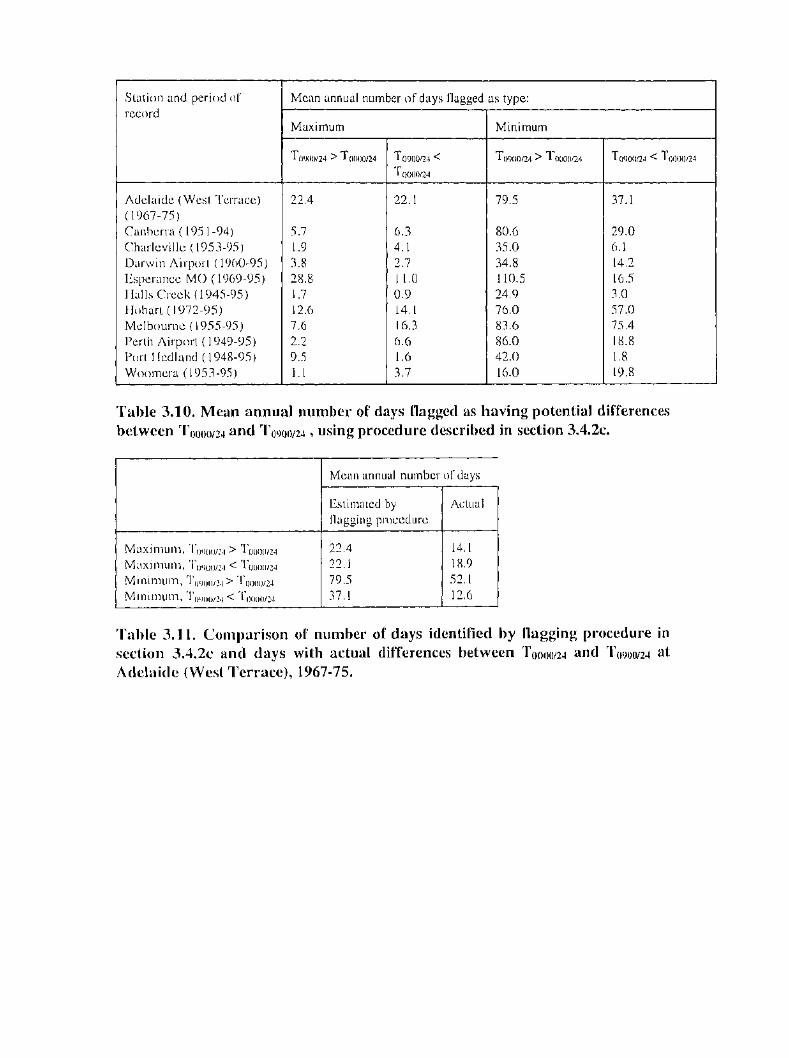
Station and period of Mean annual number of days tlagged as type: record
Maximum Minimum
T OIJ00/24 > T 0000/24 To9oo124 < To900I24 > Toooot24 T o<Joot24 < T oooot24
Toooot24
Adelaide (West Terrace) 22.4 22.1 79.5 37.1 (1967-75) Canberra ( 195 1-94) 5.7 6.3 80.6 29.0 Charlcvillc ( 195 3-95) 1.9 4.1 35.0 6.1 Darwin Airport ( 1960-95) 3.8 2.7 34.8 14.2 Esperance MO ( 1969-95) 28.8 11.0 110.5 16.5 Halls Creek (1945-95) 1.7 0.9 24.9 3.0 Hobart ( 1972-95) 12.6 14.1 76.0 57.0 Melbourne ( 1955-95) 7.6 16.3 83.6 75.4 Perth Airport ( 1949-95) 2.2 6.6 86.0 18.8 Port Heclland ( 1948-95) 9.5 1.6 42.0 1.8 Woomera ( 1953-95) 1.1 3.7 16.0 19.8
Table 3.1 0. Mean annual number of days flagged as having potential differences between T 0ooo124 and To900/24 , using procedure described in section 3.4.2c.
Mean annual number of days
Estimated by Actual flagging procedure
Maximum, To1Joot2·1 > Toooo124 22.4 14.1
Maximum, ToiJ00/2·1 < Toooo/24 22.1 18.9
Minimum, TotJ00/2·1 > Tooool:24 79.5 52.1
Minimum, Tot>oot2-l < Toooot24 37.1 12.6
Table 3.11. C01nparison of number of days identified by flagging procedure in section 3.4.2c and days with actual differences between Toooo/24 and To900/24 at Adelaide (West Terrace), 1967-75.

minimum to be lower for a day ending at 0000 than that ending at 0900 than the
reverse, which in tum suggests that an observation day ending at 0000 will result in
lower mean minima than one ending at 0900 at these stations, although this
conclusion must be drawn with caution because the flagging procedure gives no
indication of the magnitude of the likely differences on a given day, only their
existence. Again, this is a result which is consistent with the results obtained at
Melbourne and Adelaide.
Table 3.11 shows the efficiency of the flagging procedure in detecting days when
maximum or minimum temperatures for a day ending at 0000 differ from those for a
day ending at 0900. These results suggest that the flagging procedure over-estimates
the frequency of differences, with the over-estimate being greatest for the frequency
of lower minima and higher maxima for observation days ending at 0900. This
reinforces the suggestion from Table 3.10 that using an observation day ending at
0000 will lead to a negative bias in the mean minimum temperature, relative to an
0900 observation day.
Table 3.12 gtves the mean differences between 0000, 0900 and 1nini1num
temperatures for a nutnber of stations, as well as the mean interdiurnal change in
minimum temperature, for January and July. The mean 0900 temperature is higher
than the mean 0000 temperature at most of the sites in both months, with the
exceptions being Woomera in both months, and Hobart and Melbourne in winter. The
difference is particularly marked at two of the three tropical sites, Port Hedland and ~
Halls Creek, as well as at Esperance. In the latter case, this n1ay be a consequence of
Esperance's easterly location within its time zone and its consequent early sunrise,
especially in summer. Conversely, at Melbourne and Hobart in winter, and at Darwin
(which displays a small difference all year), sunrise is relatively late. The mean
interdiumal change in minimum temperature is least in the tropics in all seasons, and
greatest about the southern coasts in summer, and the eastern inland in winter.
75

3.3.4. Implications of the results
The examination of data from Melbourne and Adelaide suggests that the 1964 change
in observation practice at those stations, from an observation day ending at 0000 to
one ending at 0900, resulted in an artificial increase in mean annual minimum
temperatures of 0.3° to 0.4°C, but no significant increase in mean annual maximum
temperatures. The frequency of high minimum temperatures shows a particularly
strong change. This, in turn, implies an artificial increase in the variability of
minimum temperature. Variability of temperature is an important factor in the
likelihood of extreme events, as is discussed in more detail in later chapters and in
Katz and Brown (1992), and the likelihood of extreme high minimum temperatures is
an impm1ant factor in human health and mortality (Karl and Knight, 1997),
particularly at a site such as Adelaide, which occasionally experiences daily minimum
temperatures in excess of 30°C.
The question arises as to how representative the Melbourne and Adelaide results are
of Australia as a whole. The results from Table 3.10 suggest that days on which daily
minimum temperatures are affected by a change in observation time arc Inost frequent
near the southern coast, and least frequent in the tropics. However, these results also
suggest that, at the southern coastal sites, the large number of days when the
minimum temperature for a day ending at 0000 is lower than that for a day ending at
0900 is partially offset by the larger number of days when it is higher. It is entirely
possible that the magnitude of the temperature bias at Port Hedland, where total
number of days affected by a change in observation time is smaller but days when the
minimum temperature for a day ending at 0000 is higher than that at 0900 are very
rare, may be similar to that at the southern stations, but no data exist to test this
proposition objectively. Nevertheless, the 0000 and 0900 temperatures and the
interdi umal temperature changes outlined in Table 3.12 suggest that it is most
probable that the time of observation bias is greatest in southern Australia, and
consequently that the Adelaide and Melbourne results are at the high end of the range
which is likely to exist over Australia as a whole.
76

Station name January July
Mean Mean Mean interdiumal Time of Mean Mean Mean interdiurnal Time of difference (°C) difference (°C) change in minimum sunrise (LST) difference (°C) difference (°C) change in minimum sunrise (LST)
( to900 - T o900m) ( 1:oooo - T 0900f:'A) temperature (°C) ( to900 - T o900124) ( toooo - T o900r.!-4) temperature (°C)
Adelaide (Kent 4.5 3.2 2.8 0618* 2.8 2.2 2.2 0721 Town) Canberra 4.8 3.8 2.5 0604* 3.8 3.3 2.7 0710 Charleville 5.9 3.9 2.0 0536+ 6.2 4.3 2.6 0702 Darwin AP 3.1 2.2 1.5 0632 3.4 2.8 1.1 0709 Esperance MO 5.9 1.8 2.4 0457+ 3.2 2.1 2.0 0655 Halls Creek 6.1 3.0 1.7 0506+ 7.9 4.1 1.7 0601 Hobart 3.6 2.1 2.1 0551* 2.0 2.4 1.9 0737 Melbourne 3.2 3.2 2.4 0615* 1.8 2.3 2.0 0733 Perth AP 6.8 3.8 2.4 0526+ 3.4 2.6 2.1 0715 Port Hedland 6.4 2.2 1.3 0538+ 8.2 3.0 1.9 0641 Woomera 4.1 5.0 2.6 0634* 3.4 3.6 1.9 0719
*Daylight saving in use throughout period: time shov.n is daylight saving time. +Daylight saving in use for a short part of the period: time shmvn is standard time.
Table 3.12. Difference between mean temperatures at 0000 and 0900 and mean 24-hour minimum temperature (T 0900124), mean interdiurnal change in minimum temperature, and local time of sunrise for the 15th of each month, for period 1972-1996 (1977 ~ 1996 at Adelaide)
i
I
I
'
I

When historical data are being examined, the extent of the influence of the time of
observation bias will also be affected by the number of stations that were actually
using an observation day ending at 0000 prior to 1964. As noted in section 3.3.1., the
observation day ending at 0000 was only used at first-order stations, and not all of
them followed the procedure rigorously. Many of the co-operative stations, which
form the bulk of the Australian temperature station network, used, in effect, a
minimum temperature for the 18 hours ending at 0900. The results from Melbourne in
Table 3.9 suggest that the positive bias frotn using an 18-hour minimum ending at
0900, at that site at least, is of comparable magnitude to the negative bias from using a
24-hour minimum ending at 0000. It follows from this that the impact on long-term
temperature trends at a patticular stations could be significant, but, when averaged
spatially, the opposite biases will tend to cancel each other out to some extent. A
regional bias could still arise, as first-order stations tended to be 1nore concentrated in
coastal areas than co-operative stations were, especially before the opening of a large
number of airport meteorological offices during the Second World War.
The implications of the proposal to change the observation time in eastern Australia to
2100 UTC (0700 LST in winter, 0800 in sum1ner in those states which observe
daylight saving) are also worthy of examination. Mitchell (1958) has already noted
that the mean temperature is particularly sensitive to observation time changes around
sunrise, and 2100 UTC is within 30 minutes of sunrise in winter in much of eastern
Australia. In the worst-case scenario, where one assumes that the tin1c of observation
coincides with the time of minimum temperature, on any day when the overnight
minimum temperature on one day is higher than it has been the previous day, the 24-
hour n1inimum on that day will be biased downwards by the difference between the
overnight mini mum temperatures on the two days, as the cooler first day is effectively
counted twice.
As such a situation would be expected to arise on 50% of days, the expected
difference between the overnight minimum and 24-hour minitnum would be half the
mean interdiurnal temperature change as shown in Table 3.12. Combining this with
the difference between the mean overnight and 24-hour 1ninima (Table 3.9), the
interdiumal temperature change in some areas approaches 3°C, suggesting that the
77

potential exists for a bias in the vicinty of -1 oc in minimum temperatures in some
areas if a change to an observation day ending at 2100 UTC takes place.
3.4. Biases arising from the use of accumulated data
Ideally, all data sets used in a study would be complete. In practice, there is no long
term station in Australia that has no missing days in its record, and hence it is
necessary to consider the implications of missing data for the overall temperature
record.
Missing data can take one of two forms:
1. An observation is missed.
2. An observation is taken but is found to be faulty, or is not communicated (in the
case of an automatic station where there is no manual record to act as a back-up).
Missing data of the second type should not affect the overall temperature record, as
long as there is no systematic bias in the type of days on which observations are
missed. This may not be the case if observations are more likely to be missed under
extreme conditions, although it seems reasonable to surmise that cornmunications
failures or the like are more likely to happen in extreme rainfall or wind than they are
in extreme temperatures. (Robinson (1990) noted a potential for data loss during
extreme conditions at automatic stations, due to power outages). A tendency towards
missing data occuning under particular te1nperature conditions could also result from
missing weekend data, as a number of authors, such as Simmonds and Kaval (1986)
and Simmonds and Keay ( 1997), have found a relationship between temperature and
day of the week. In such cases the deletion of a particular day of the week on a
consistent basis could lead to a bias in mean temperatures.
The first type of missing data, which is by far the more common, is of more concern.
If the observation is missed then the thermometers are not reset, and hence the
maximum and minimum temperatures which are recorded when the thermometers are
eventually read are the minimum and maximum temperatures for the previous 48
78
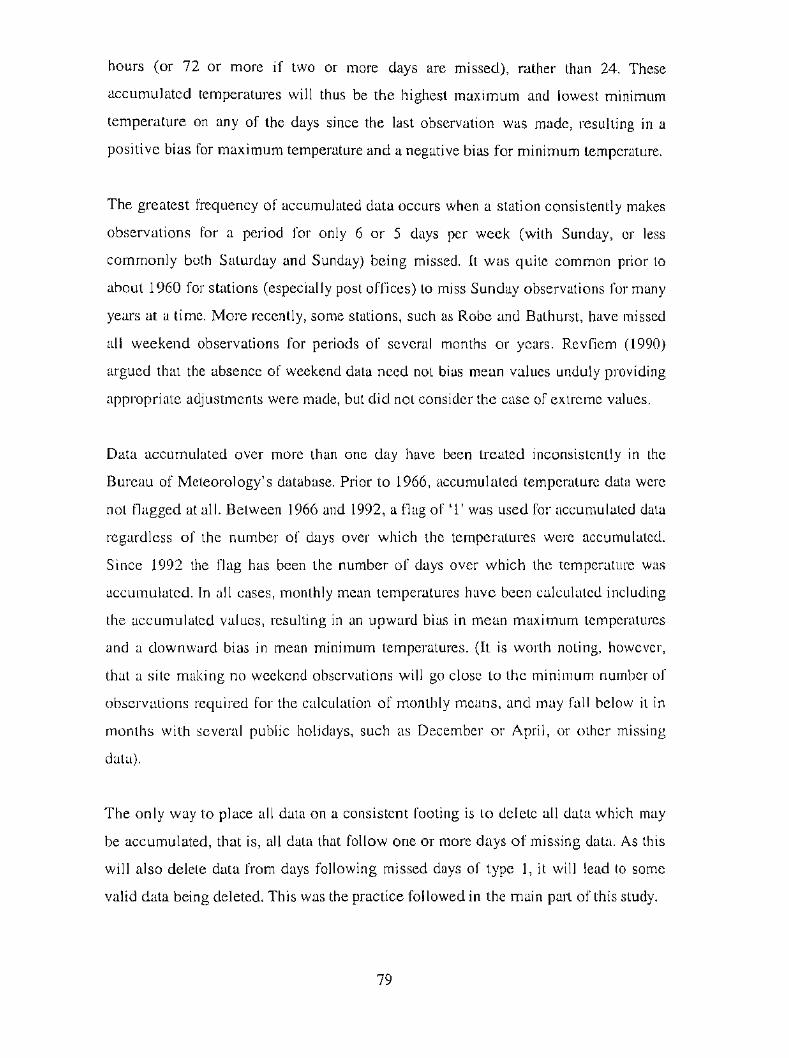
hours (or 72 or more if two or more days are missed), rather than 24. These
accumulated temperatures will thus be the highest maximum and lowest minimum
temperature on any of the days since the last observation was made, resulting in a
positive bias for maximum temperature and a negative bias for minimum temperature.
The greatest frequency of accumulated data occurs when a station consistently makes
observations for a period for only 6 or 5 days per week (with Sunday, or less
commonly both Saturday and Sunday) being missed. It was quite common prior to
about 1960 for stations (especially post offices) to miss Sunday observations for many
years at a time. More recently, some stations, such as Robe and Bathurst, have missed
all weekend observations for periods of several months or years. Revfiem (1990)
argued that the absence of weekend data need not bias mean values unduly providing
appropriate adjustments were made, but did not consider the case of extreme values.
Data accumulated over more than one day have been treated inconsistently in the
Bureau of Meteorology's database. Prior to 1966, accumulated temperature data were
not flagged at all. Between 1966 and 1992, a flag of' 1' was used for accumulated data
regardless of the number of days over which the temperatures were accumulated.
Since 1992 the flag has been the number of days over which the temperature was
accutnulated. In all cases, tnonthly mean temperatures have been calculated including
the accumulated values, resulting in an upward bias in mean maximum temperatures
and a downward bias in mean minimum temperatures. (It is worth noting, however,
that a site making no weekend observations will go close to the minimum number of
observations required for the calculation of monthly means, and tnay fall below it in
months with several public holidays, such as December or April, or other missing
data).
The only way to place all data on a consistent footing is to delete all data which may
be accumulated, that is, all data that follow one or more days of missjng data. As this
will also delete data from days following missed days of type 1, it will lead to some
valid data being deleted. This was the practice followed in the main part of this study.
79

3.4.1. Quantification of biases arising from use of accumulated temperatures
There are two feasible approaches to the investigation of accumulated temperatures.
1. Use a reasonably complete data set and delete data for each Sunday (or Saturday
and Sunday), adjusting maxima and minima on Monday to be the equivalent of
accumulated data for 48 or 72 hours.
2. Examine a data set with a substantial amount of accumulated data and investigate
whether there is any significant difference between the temperatures recorded on days
with accumulated temperatures and temperatures on other days.
Both approaches were used in this section.
The results of the first approach are given in Tables 3.13 and 3.14. All available
Bureau-operated sites were used in this part of the study (these being chosen because
of their generally small amount of missing data). If only Sunday observations are
missing and the Monday temperature is accumulated over 48 hours, this results in a
bias of between +0.1 o and 0.3°C for maximum temperature and between -0.1 and -
0.3°C for minimum temperature at most stations, although the bias for maximum
temperature reaches +0.43°C at Ceduna in January. The bias is least in the tropics,
especially near the coasts, and greatest near southern coasts for maxima and in the
southern inland for minima. The bias for maximum temperature shows a marked peak
at most stations in spring and summer, and, for minimum temperature, a less
pronounced peak in winter and spring. As the biases for maximum and minimum
temperature are of opposite sign, there will be a particularly marked bias for the mean
diurnal temperature range, reaching +0.73°C at Ceduna in October.
The biases arising from removing all weekend observations and accumulating
Monday temperatures over 72 hours, as would be expected, have a similar spatial and
seasonal distribution to those arising from the absence of Sunday observations only,
but are of approximately double the magnitude. The bias for spring and summer
maxima exceeds +0.6°C at a number of southern stations and reaches +0.92°C at
80

Station name Bias (°C)
January April July October
Maximum Minimum DTR Maximum Minimum DTR Maximum Minimum DTR Maximum Minimum DTR
Halls Creek 0.16 -0.10 0.26 0.07 -0.07 0.14 0.10 -0.16 0.26 0.07 -0.15 0.22 Broome 0.13 -0.13 0.29 0.09 -0.08 0.17 0.13 -0.16 0.29 0.14 -0.13 0.27 Port Hedland 0.16 -0.12 0.28 0.10 -0.09 0.19 0.12 -0.18 0.30 0.19 -0.14 0.33 Leannonth 0.14 -0.07 0.21 0.13 -0.08 0.21 0.10 -0.16 0.26 0.22 -0.12 0.34 Carnarvon 0.23 -0.10 0.33 0.16 -0.13 0.29 0.12 -0.13 0.25 0.15 -0.16 0.31 Meekatharra 0.14 -0.21 0.35 0.20 -0.14 0.34 0.18 -0.13 0.31 0.21 -0.23 0.44 Geraldton 0.32 -0.21 0.53 0.20 -0.17 0.37 0.13 -0.13 0.26 0.22 -0.24 0.46 Perth Airport 0.29 -0.21 0.50 0.18 -0.18 0.36 0.14 -0.18 0.32 0.23 -0.22 0.45 Albany 0.30 -0.22 0.52 0.24 -0.19 0.43 0.15 -0.20 0.35 0.15 -0.24 0.39 Esperance 0.39 -0.21 0.60 0.31 -0.17 0.48 0.19 -0.17 0.36 0.26 -0.23 0.49 Forrest 0.38 -0.17 0.55 0.30 -0.20 0.50 0.20 -0.20 0.40 0.31 -0.35 0.66 Kalgoorlie 0.29 -0.22 0.51 0.27 -0.15 0.42 0.20 -0.22 0.42 0.29 -0.25 0.54 Giles 0.15 -0.13 0.28 0.20 -0.11 0.31 0.18 -0.17 0.35 0.20 -0.30 0.50 Darwin Airport 0.10 -0.12 0.22 0.07 -0.08 0.15 0.08 -0.11 0.19 0.09 -0.09 0.18 Alice Springs 0.13 -0.22 0.35 0.18 -0.17 0.35 0.21 -0.20 0.41 0.30 -0.25 0.55 Woomera 0.26 -0.19 0.45 0.22 -0.14 0.36 0.17 -0.15 0.32 0.31 -0.24 0.55 Ceduna 0.43 -0.22 0.65 0.28 -0.29 0.57 0.18 -0.22 0.40 0.39 -0.34 0.73 Adelaide RO 0.32 -0.25 0.57 0.23 -0.24 0.47 0.13 -0.17 0.30 0.38 -0.25 0.63 Mount Gambier 0.36 -0.27 0.63 0.21 -0.21 0.42 0.11 -0.19 0.30 0.28 -0.22 0.50 Thursday Island 0.09 -0.04 0.13 0.08 -0.02 0.10 0.04 -0.07 0.11 0.03 -0.05 0.08 Cairns 0.10 -0.07 0.17 0.11 -0.07 0.18 0.09 -0.13 0.22 0.07 -0.12 0.19 Townsville 0.10 -0.07 0.17 0.09 -0.09 0.18 0.10 -0.19 0.29 0.06 -0.13 0.19 Mackay MO 0.08 -0.12 0.20 0.07 -0.08 0.15 0.12 -0.18 0.30 0.06 -0.13 0.19 Longreach 0.09 -0.15 0.24 0.10 -0.15 0.25 0.17 -0.19 0.36 0.22 -0.17 0.39 Rockhampton 0.14 -0.09 0.23 0.11 -0.11 0.22 0.17 -0.22 0.39 0.13 -0.16 0.29 Amberley 0.16 -0.12 0.28 0.12 -0.12 0.24 0.13 -0.23 0.36 0.23 -0.21 0.44 Brisbane AP 0.11 -0.09 0.20 0.11 -0.08 0.19 0.12 -0.15 0.27 0.17 -0.14 0.31 Charleville 0.16 -0.16 0.32 0.14 -0.21 0.35 0.16 -0.22 0.38 0.22 -0.21 0.43
Table 3.13. Biases in mean maximum and minimum temperature and diurnal temperature range if Sunday observations missing

Table 3.13 (cont.). Biases in mean maximum and minimum temperature and diurnal temperature range if Sunday observations
.A..A. ........ Ol.J..&..LI..~
Station name Bias (°C)
January April July October
Maximum Minimum DTR Maximum Minimum DTR Maximum Minimum DTR Maximum Minimum DTR
Co bar 0.21 -0.22 0.43 0.14 -0.20 0.34 0.16 -0.15 0.31 0.32 -0.17 0.49
Moree 0.18 -0.15 0.33 0.11 -0.21 0.32 0.18 -0.23 0.41 0.28 -0.22 0.50 I
Coffs Harbour 0.14 -0.12 0.26 0.15 -0.17 0.32 0.12 -0.22 0.34 0.21 -0.19 0.40
Williamtown 0.26 -0.16 0.42 0.19 -0.18 0.37 0.18 -0.19 0.37 0.29 -0.22 0.51
SydneyRO 0.24 -0.12 0.36 0.18 -0.11 0.29 0.14 -0.12 0.26 0.25 -0.16 0.41
Richmond 0.26 -0.20 0.46 0.22 -0.19 0.41 0.15 -0.21 0.36 0.30 -0.22 0.52
Nowra 0.24 -0.18 0.42 0.22 -0.17 0.39 0.11 -0.15 0.26 0.33 -0.21 0.54
CanberraAP 0.24 -0.21 0.45 0.18 -0.17 0.35 0.15 -0.21 0.36 0.20 -0.27 0.47
Wagga Wagga 0.26 -0.25 0.51 0.15 -0.22 0.37 0.16 -0.16 0.32 0.22 -0.24 0.46
Mil dura 0.29 -0.21 0.50 0.24 -0.18 0.42 0.15 -0.16 0.31 0.30 -0.24 0.54
Sale 0.31 -0.19 0.50 0.22 -0.20 0.42 0.14 -0.21 0.35 0.29 -0.22 0.51
Melbourne RO 0.40 -0.19 0.59 0.23 -0.18 0.41 0.14 -0.17 0.31 0.30 -0.24 0.54
Laverton 0.36 -0.21 0.57 0.23 -0.25 0.48 0.11 -0.19 0.30 0.32 -0.22 0.54
Launceston AP 0.21 -0.26 0.47 0.20 -0.23 0.43 0.11 -0.23 0.34 0.17 -0.21 0.38
HobartRO 0.27 -0.20 0.47 0.25 -0.20 0.45 0.13 -0.18 0.31 0.30 -0.17 0.47
J

Station name Bias (°C)
January April July October
Maximum Minimum DTR Maximum Minimum DTR Maximum Minimum DTR Maximum Minimum DTR
Halls Creek 0.27 -0.19 0.46 0.13 -0.19 0.32 0.20 -0.31 0.51 0.17 -0.30 0.47 Broome 0.26 -0.24 0.50 0.20 -0.16 0.36 0.25 -0.30 0.55 0.35 -0.22 0.57 Port Hed1and 0.34 -0.25 0.59 0.22 -0.16 0.38 0.18 -0.34 0.52 0.43 -0.27 0.70 Learrnonth 0.27 -0.17 0.44 0.25 -0.20 0.45 0.18 -0.31 0.49 0.40 -0.28 0.68 Carnarvon 0.51 -0.18 0.69 0.36 -0.23 0.59 0.25 -0.24 0.49 0.35 -0.32 0.67 Meekatharra 0.29 -0.40 0.69 0.41 -0.25 0.66 0.36 -0.24 0.60 0.41 -0.48 0.89 Gerald ton 0.67 -0.35 1.02 0.46 -0.35 0.81 0.24 -0.28 0.52 0.43 -0.46 0.89 Perth Airport 0.61 -0.38 0.99 0.47 -0.38 0.85 0.27 -0.34 0.61 0.44 -0.42 0.86 Albany 0.67 -0.41 1.08 0.46 -0.39 0.85 0.30 -0.38 0.68 0.36 -0.44 0.80 Esperance 0.89 -0.39 1.28 0.63 -0.37 1.00 0.38 -0.34 0.72 0.62 -0.42 1.04 Forrest 0.74 -0.35 1.09 0.65 -0.37 1.02 0.39 -0.38 0.77 0.71 -0.62 1.33 Kalgoorlie 0.62 -0.40 1.02 0.56 -0.31 0.87 0.38 -0.42 0.80 0.62 -0.49 1.11 Giles 0.29 -0.30 0.59 0.37 -0.22 0.59 0.32 -0.31 0.63 0.49 -0.54 1.03 Darwin Airport 0.20 -0.22 0.42 0.16 -0.15 0.31 0.16 -0.21 0.37 0.16 -0.17 0.33 Alice Springs 0.25 -0.48 0.73 0.36 -0.36 0.72 0.41 -0.41 0.82 0.64 -0.52 1.16 Woomera 0.47 -0.42 0.89 0.41 -0.33 0.74 0.31 -0.30 0.61 0.75 -0.41 1.16 Ceduna 0.90 -0.54 1.44 0.59 -0.54 1.13 0.36 -0.39 0.75 0.92 -0.63 1.55 Adelaide RO 0.63 -0.51 1.14 0.42 -0.33 0.75 0.23 -0.33 0.56 0.90 -0.40 1.30 Mount Gambier 0.76 -0.49 1.25 0.45 -0.41 0.86 0.21 -0.39 0.60 0.61 -0.40 l.Ol Thursday Island 0.30 -0.08 0.38 0.14 -0.06 0.20 0.08 -0.11 0.19 0.07 -0.11 0.18 Cairns 0.20 -0.15 0.35 0.19 -0.14 0.33 0.18 -0.27 0.45 0.12 -0.24 0.36 Townsville 0.19 -0.15 0.34 0.16 -0.18 0.34 0.20 -0.41 0.61 0.13 -0.29 0.42 MackayMO 0.17 -0.21 0.38 0.15 -0.20 0.35 0.23 -0.35 0.58 0.13 -0.27 0.40 Longreach 0.26 -0.27 0.53 0.20 -0.28 0.48 0.35 -0.31 0.66 0.41 -0.37 0.78 Rockhampton 0.27 -0.19 0.46 0.22 -0.19 0.41 0.30 -0.43 0.73 0.26 -0.34 0.60 Amberley 0.34 -0.26 0.60 0.22 -0.23 0.45 0.23 -0.38 0.61 0.41 -0.44 0.85 Brisbane AP 0.23 -0.19 0.42 0.20 -0.14 0.34 0.20 -0.28 0.48 0.19 -0.31 0.60 Charlevil1e 0.35 -0.30 0.65 0.29 -0.37 0.66 0.30 -0.45 0.75 0.46 -0.46 0.92
-·--
Table 3.14. Biases in mean maximum and minimum temperature and diurnal temperature range if Saturday and Sunday observations missing
I I
I
Table 3.14 (cont.). Biases in mean maximum and.minimum temperature and diurnal temperature range if Saturday and Sunday
UU~CJ. l' Cl.L.lVII~ ••u.~u.o..o..ll.j;
Station name Bias (°C)
January April July October
Maximum Minimum DTR Maximum Minimum DTR Maximum Minimum DTR Maximum Minimum DTR
Co bar 0.44 -0.47 0.91 0.27 -0.41 0.68 0.30 -0.32 0.62 0.66 -0.33 0.99
Moree 0.40 -0.36 0.76 0.21 -0.39 0.60 0.34 -0.40 0.74 0.52 -0.48 1.00
Coffs Harbour 0.29 -0.28 0.57 0.29 -0.28 0.57 0.24 -0.38 0.62 0.38 -0.43 0.81
Williailltown 0.56 -0.31 0.87 0.40 -0.31 0.71 0.29 -0.32 0.61 0.56 -0.47 1.03
SydneyRO 0.48 -0.25 0.73 0.39 -0.21 0.60 0.27 -0.23 0.50 0.50 -0.32 0.82
Richmond 0.55 -0.37 0.92 0.43 -0.37 0.80 0.27 -0.35 0.62 0.58 -0.49 1.07
Nowra 0.47 -0.36 0.83 0.49 -0.33 0.82 0.22 -0.27 0.49 0.61 -0.40 1.01
CanberraAP 0.50 -0.42 0.92 0.37 -0.39 0.76 0.26 -0.40 0.66 0.41 -0.51 0.92
Wagga Wagga 0.49 -0.51 l.OO 0.31 -0.40 0.71 0.29 -0.34 0.63 0.47 -0.46 0.93
Mil dura 0.62 -0.42 1.04 0.46 -0.39 0.85 0.30 -0.34 0.64 0.69 -0.43 1.12 I Sale 0.67 -0.42 l.09 0.45 -0.40 0.85 0.27 -0.34 0.61 0.61 -0.46 1.07
Melbourne 0.86 -0.37 1.23 0.48 -0.35 0.83 0.27 -0.32 0.59 0.64 -0.43 1.07 I I
Laverton 0.77 -0.40 1.17 0.41 -0.45 0.86 0.23 -0.36 0.59 0.68 -0.38 1.06
Launceston AP 0.39 -0.46 0.85 0.34 -0.44 0.78 0.22 -0.38 0.60 0.36 -0.44 0.80
Hobart RO 0.59 -0.40 0.99 0.49 -0.37 0.86 0.27 -0.31 0.58 0.59 -0.33 0.92

Ceduna in October, while for minima the same station has an October bias of -0.63°C,
leading to a bias of+ 1.55°C for the mean diurnal temperature range.
In the second approach, data from two stations with missing Sunday data were
examined. The stations used were Wyalong (1959-64) and Tewantin ( 1957-61 ). These
stations were chosen during these periods because they were missing all Sunday
observations but few other observations. Table 3.15 shows a comparison between
observations on the day after missing data at these stations (mostly Mondays) and all
other days. On the assumption that one observation in six is accumulated, the
estimated bias in mean rnaximum and minimum temperatures will be one-sixth of the
mean difference between the two types of observations. Given this, the estimated bias
at Tewantin is +0.14°C for annual mean maxima and -0.23°C for annual tnean
minima, while at Wyalong the values are +0.l9°C and -O.l3°C respectively. These
results are of similar magnitude to those shown in Table 3.13 for stations in
comparable regions (coastal southern Queensland and inland New South Wales).
3.4.2. Implications of the use of accumulated data
The greatest impact of the use of accumulated data is on the diurnal tctnperature
range, as the upward bias in maximum temperature and the downward bias in
minimum temperature are added to each other. (Conversely, when mean ten1peratures
are calculated the biases counteract each other). This is of particular potential
importance for a number of reasons. Firstly, one of the more pronounced trends in
global temperature that has been found in a number of studies is a reduction in the
mean diurnal temperature range (e.g. Easterling et al., 1997), and Torok (1996) found
a decrease of 0.48°C in the mean Australian diurnal temperature range since 1910.
Secondly, the biases found in this section, when applied to maximum and minimum
temperatures separately, are at or near the lower limit of the magnitude of
discontinuity detectable by the techniques used in this study (being mostly in the
order of O.l oc to 0.3°C when one day per week is missing), yet, when they are
combined, the resultant bias is between 0.2°C and 0.6°C at most stations.
81
The mean monthly maximum and minimum temperatures in the Bureau of
Meteorology's database are, as mentioned earlier, calculated with accumulated data
included. The task of identification of months with accumulated data is made more
difficult by the fact that the number of days with observations is not available in the
database prior to 1957 at most stations, and hence periods of the record when
weekend data are missing at a station can only be identified by examining the daily
manuscript records from that station. One possible solution for the identification of
such periods could be to carry out the tests used in Chapter 4 for the detection of
inhomogeneities on the diurnal temperature range as well as maximum and minimum
temperature.
In the worst-case scenario, in which all data at the start of the record were missing
Sunday observations and none at the end were, the artificial trend in the di umal
temperature range would be of comparable magnitude to the trend observed by Torok
(1996). In practice, it is unlikely that this would be the case, as not all stations would
have missed Sunday observations. The pre-1957 manuscript data that has been
obtained suggests that missing Sunday data were most common between about 1920
and 1960, with fewer missed days before and after, and that the observation were
mostly missed at post offices and similar sites; lighthouses and similar sites, which
make up a large part of the coastal observing network, rarely missed days. The impact
of accumulated data on the observed trend in mean diurnal temperature range over
Australia as a whole is worthy of further investigation, although it is outside the direct
scope of this thesis.
3.5. Summary
Three systematic issues affecting the development of homogeneous, high-quality data
sets have been addressed in this chapter. These serve as a precursor to the
development of the data set in Chapter 4. The potential dependence of the magnitude
of temperature discontinuities upon the position of a day in the frequency distribution
of temperature, as described in section 3.2, is particularly crucial in the development
of a homogeneous time series of extreme events. In Chapter 4, the methods developed
in section 3.2 are applied to the development of a comprehensive data set.
82
•

Month Station name
Wyalong Tewantin
Maximum Minimum Maximum Minimum
January +0.26 -0.76 +0.68 -0.92 February + 1.15 -2.20 +0.41 -0.66 March +0.78 +0.29 -0.09 -1.60 April +1.52 -0.86 +0.98 -0.06 May +0.58 -0.56 +0.80 -1.39 June +0.72 -1.18 +0.08 -2.34 July +0.79 -0.07 +1.32 -1.21 August + 1.16 -0.44 +0.14 -1.87 September +0.58 -1.27 +0.98 -1.07 October +1.42 -0.28 +2.31 -2.16 November +1.74 -1.54 +0.69 -2.07 December +2.97 -0.31 +1.62 -1.17
Annual +1.14 -0.76 +0.83 -1 J8
Table 3.15. Mean temperature difference (°C) between days following n1issing data and all other observations for Wyalong (1959-64) and Tewantin (1957-61)
Chapter 4
The Development of a High-Quality Daily Temperature Data
Set for Australia
4.1. Introduction to the problem of developing high-quality daily temperature data
The development of high-quality temperature data sets, as noted in Chapter 1, is a
problem which has received considerable attention in recent years. The major works in
this field in Australia have been those of Torok (1996) and Torok and Nicholls (1996).
Their work has been focused on data at the annual timescale. This has also been the case
with much of the work undertaken outside Australia. There has been some attention given
to data at the seasonal or monthly timescale, but this has involved similar methods to
those used for homogenisation of annual data.
The development of daily temperature tiJne series involves a more complex set or
problems than those involved in developing annual or seasonal series. Daily time series
are much more susceptible to short-term gross en·ors than are monthly or annual means.
A 5°C CITor in a single maximum or minimum temperature will have a minimal impact
on a monthly, seasonal or annual mean, but it tnay be critical when extreme ten1perature
events are being examined. Furthermore, as was discussed in section 3.2, the methods
used to homogenise annual or seasonal mean temperatures once a discontinuity is
identified n1ay not be appropriate for the homogenisation of daily maximum and
minimun1 temperatures, as they generally take no account of possible changes in the
variability of temperature, only in its mean.
The inherent problems in developing high-quality daily temperature data sets may be
divided into two categories: long-term systematic inhomogeneities and short-term errors.
83

4.1.1. Long-term systematic inhomogeneities
The following are examples from an extensive list of potential systematic
inhomogeneities which are discussed by Torok (1996). A more detailed description of
these factors may be found there.
Station moves: These are relatively common throughout the period of record. In
particular, many stations have moved from town centres to airports, as urban sites have
become built up and aviation has become an important user of meteorological
information. This process was most frequent during the 1940's and 1950's, but is
continuing to the present day. Of the stations used in this study, Charters Towers, St.
George, Walgett and Bourke all moved to airpmis between 1992 and the end of the data
set in 1996.
There is also a long-term Bureau policy to reduce the number of observations at post
offices, at which many stations are located. Stations located on private land are
susceptible to moves when properties change hands or observers cease making
observations for any reason.
Small-scale relocations of instruments within the same general area are also quite
common. These may have a significant impact on observed temperatures if the
characteristics of the new site are different (see below).
Station relocations are a particularly significant issue in locations where there are strong
local temperature gradients, such as near coasts or in hilly terrain.
Instrument changes: The Stevenson Screen has been a standard throughout Australia for
most of the 20th century. Prior to the formation of the Commonwealth Bureau of
Meteorology in 1908, a wide variety of screens were in use, making comparisons
difficult, both in time and space. While this is a real problem in attempting to extend the
Australian climate record back into the 19th century, the limited availability of digitised
daily data means that a very limited amount of pre-1908 data has been used in this study.
84

A more recent change has been the move to automatic weather stations. The Bureau is
installing approximately 35 automatic weather stations per year, some in new sites and
some in place of existing sites. Where automatic stations have been installed in place of
manual sites, there has often been a period of dual observations maintained at the two
sites. Four of the stations in this study were automated (Forrest, Cape Otway, Tewantin
and Oodnadatta) prior to the end of this study in December 1996, all of them since late
1994. At present, this affects only a small proportion of stations for a very short part of
their record, but the process has continued since 1996 and it is likely that the majority of
stations in this data set will be using automated observations by 2005. The majority of
alpine temperature observations are already automated.
Poorly maintained equipment (such as a screen becoming discoloured, rather than white
as per specifications) could also have an impact on observed temperatures.
Changes in site environment: Even where the location or a site has remained
unchanged, the local enviromnent around a site may change. Common causes of this
include building around instrument sites, or growth (or removal) of vegetation in the
vicinity of instruments. Building around instrument sites has been particularly common at
rural post office sites, which arc often located in town centres. This includes the
construction of asphalt car parks adjacent to sites (Annidale and Glen Innes are examples
of this).
The issue of urbanisation as an influence on the climate record is a separate issue. It is
well-established that urban centres are likely to experience warmer 111inimum
temperatures than surrounding rural areas (the so-called "urban heat island"), with the
magnitude of the urban heat island being a function of the town or city's population (e.g.
Karl et al., 1988). For the purposes of a study such as this, any change in the magnitude of
the urban heat island over time is of greater importance than the existence of an urban
heat island per se. Thus, for those stations for which daily records are only available for
the period since 1957 (as is the case for the majority of stations used in this study), the
stations of greatest concern are those located in or near the centres of towns that have
85
---seen significant growth between 1957 and the present.
A population of 10,000 has often been taken as the lower limit for significant
urbanisation effects, although noticeable urban heat islands have been found in much
smaller centres (Torok et al., 2001). The following stations used in this study can be
considered to have been affected by urbanisation:
1. In major city: Sydney, Melbourne, Adelaide (both sites), Hobart.
2. Away from centre of major city but within general metropolitan area: Laverton,
Richmond (NSW), Perth Airport, Brisbane Airport, Darwin Airport.
3. In or near centre of country town with population exceeding 10,000: Dubbo, Port
Lincoln, Tewantin, Port Macquarie.
4. Has moved from centre of town with population exceeding 10,000 to airport during
period of record used in study: Albany, Bundaberg.
A categorisation of all station locations may be found in Table 2.1 a.
It should be noted at this point that the existence of an artificial temperature trend due to
urbanisation at an individual station does not exclude it from consideration in this study;
rather, it is an aid to interpretation of observed trends at those stations. It is, however,
invalid to interpret observed trends at an urban station as being representative of
conditions over a broader region.
Changes in observation practices: The principal problems here arise from changes in
the time of observation, and changes in the frequency of missed observations (for
example, taking/not taking Sunday observations). These were both discussed at some
length in Chapter 3.
The Bureau of Meteorology adopted the Celsius scale of temperature measurement on
September 1, 1972. While a discontinuity in the relationship between mean maximum
temperatures and annual rainfall over Australia has been observed around this time
(Nicholls et al., 1996a), there is no evidence that the change in units (and the consequent
86

change of thermometers) was responsible for that discontinuity.
Observers are instructed to make observations to the nearest 0.1 degree Celsius, and prior
to metrication were instructed to make observations to the nearest 0.1 degree Fahrenheit.
In practice, as the figures in Tables 4.1a, 4.1 b and 4.lc demonstrate, many observers,
ptior to 1972, observed temperatures only to the nearest whole degree. This practice has
become less common since 1972, although there continues to be a bias towards
observations ending in .0, something that has also been noted outside Australia (Nese,
1994; Petrovic, 1998). In addition, at present, maximum and minimum temperatures
from some automatic weather stations are only archived to the nearest whole degree, as a
result of limitations in the codes used for transmission (Wong, pers. comm.).
While mistakes, and failure to observe standards of observation, by observers can result
in long-term systematic biases, they more commonly result in short-term errors and are
dealt with in that section.
4.1.2. Short-tern1 errors
These are errors that affect observations either on a single day or over a period of a few
weeks or months. Unless they are especially large, such errors will not have a substantial
effect on mean annual tetnperatures, but they may be critical in an ex ami nation of
extremes.
Errors of this type include:
Observer errors: Observer eJTors recorded include the misreading of thermometers by 5
or 10 degrees, reading the wrong end of the index for maximum and minimum
thermometers, failing to reset the thermometers each day, or recording some other climate
element (such as the temperature at 0900 or the grass minimum temperature) as the
maximum or minimum temperature. These errors were usually isolated, but occasionally
persist over a longer period (e.g. Thargomindah in January-February 1963), possibly at
times when the regular observer was absent.
87

Clerical errors: Data received by the Bureau and entered into its computer system were
normally keyed twice, until the introduction of improved data management and quality
control software in 1994, to minimise the risk of typographical errors in processing
(Hutchinson, pers. comm .. ). Nevertheless, processing errors still occurred, especially as
the legibility of the handwriting of some observers leaves something to be desired.
Defective instruments: It was not unknown for an instrument to develop a fault, but for
some time to elapse between the fault's occurrence and the removal or replacement of the
defective instrument. The observed temperatures would therefore be suspect in the
intervening period. Torok (1996) notes that the minimum thermometer was particularly
vulnerable to faults, and was also less readily replaced than maximum thermometers
were. There are, accordingly, more breaks in the minimum temperature record than there
are for maximum temperature, especially in remote areas.
4.2. Techniques of development of high-quality temperature data sets
The technique used to develop high-quality sets of daily temperature data consisted of
three principal steps. These steps were:
1. A first pass of detection of single-day errors, in order to remove obvious errors from
the data sets prior to any attempts to detect long-term inhomogeneities.
2. The identification of, and adjustment for, inhomogeneities in the long-term data sets
after gross errors had been removed.
3. Spatial analysis of the adjusted temperature data in order to identify stations whose
data differ substantially from those of its neighbouring stations.
At this point, it is important to note the distinction between rejected and flagged data.
Data may be rejected immediately if it violates a condition which must hold (e.g.
maximum 2 minimum). Data which are identified by some of the tests outlined below
(e.g. for differing by more than a set amount from its neighbours) are flagged for further
examination. This may lead to its ultimate deletion but does not necessarily do so.
88

Station name % Of°C % Of 0 f Station name % Of°C 0( Of 0 f Station name % Of°C % Of 0 f Station name 9c of oc % Of 0 f temps temps temps temps temps temps temps temps ending in ending ending ending ending ending ending ending in .0 in .0 in .0 in .0 in .0 in .0 in .0 .0
Kalumburu 16.1 44.2 Marree 10.9 46.9 Amberley 12.4 28.9 Cabramurra 17.5 55.7 Halls Creek 13.4. 36.6 Oodnadatta A WS 13.1 26.6 Brisbane AP 12.8 29.3 Wagga Wagga 13.7 28.0 Broome 12.2 32.2 Oodnadatta PS 34.3 Tewantin PO 17.9 48.0 Wyalong 20.3 79.0 Port Hedland 11.8 27.7 Ceduna 14.9 30.6 Tewantin A \VS lOA Deni1iquin PO 10.5 63.8 Learmonth 12.2 Port Lincoln 21.0 63.2 Thargomindah 32.5 78.9 MilduraAMO 15.0 30.5 Wittenoom 13.7 61.6 Snowtown 16.8 63.9 Tibooburra 16.5 87.9 Nnill 28.2 68.1 Carnarvon 13.6 29.5 Adelaide (\VTJ 15.3 20.4 \Vi1cannia 21.0 99.7 Kerang 21.0 58.3 Meekatharra 12.0 31.2 Adelaide (KT) 13.3 Bourke PO 31.7 95.6 Rutherglen 26.6 77.6 Dalwallinu 25.2 58.3 Nuriootpa 17.4 28.2 Bourke AP 11.8 Gabo Island 23.7 82.4 Gerald ton 14.1 30.4 Mount Gambier 13.7 26.0 Cobar PO 93.1 Orbost 13.8 52.9 Perth Airport 11.6 27.0 Robe 25.1 61.8 Cobar MO 12.1 28.6 East Sale 12.9 30.8 Cape Leeuwin 25.4 78.5 Thursday Island 13.2 23.8 Walgett PO 24.4 82.2 \Vilsons Prom 23.3 92.2 Albany Tov,rn 51.5 Weipa comp 17.9 58.0 Walgett AP 24.8 Melbourne 12.5 26.9 AlbanyAMO 12.5 36.2 WeipaMO 14.4 Moree PO 94.7 Laverton 16.0 29.5 Esperance PO 76.2 Palmerville 53.5 96.5 Moree MO 11.7 25.7 Cape Otway 28.3 84.6 Esperance M 0 13.8 26.7 Burket0\\11 21.9 86.2 Gunnedah 11.3 30.3 Low Head 41.1 87.5 Cunderdin 21.2 42.6 Richmond tQ1d.) 26.3 65.7 Inverell PO 16.3 62.6 Launceston AP 15.3 32.5 Wandering 22.4 53.5 Cairns 13.8 26.4 Inverell (new) 10.7 Eddystone Point 29.6 87.4 Forrest AMO 13.4 27.5 Townsville 12.7 26.3 Yarnba 23.9 78.1 Cape Bruny 24.0 89.6 Forrest AWS 29.4 Mackay 13.1 26.8 Coffs Harbour 12.9 27.1 Hobart 13.7 28.5 Kalgoorlie 12.6 30.8 Charters T. PO 20.0 62.5 Port Macquarie 30.4 77.2 Grove 14.6 39.9 Giles 12.4 28.3 Charters T. AP 17.2 Williamtmvn 14.3 32.8 Butlers Gorge 41.0 76.9 Darwin Airport 13.0 :26.2 Barcaldine 16.5 32.7 Scone Soil Cons 15.5 29.3 Willis Island 13.8 26.5 Victoria River 24.4 4.1 Longreach AP 14.9 32.0 Bathurst ARS 24.2 61.5 Cocos Island 13.7 29.9 Dov.ns Camooweal 23.2 60.9 Dubbo 15.1 74.7 Norfolk Island 14.3 31.3 Tennant Ck PO 26.1 Birds \·i lle 26.0 93.0 Sydney 11.2 25.2 Lord Howe (old) 14.0 30.5 Tennant Ck MO 13.4 69.6 Boulia 26.4 70.9 Richmond AMO 14.1 31.5 Lord Howe 11.7 Rabbit Flat 18.9 17.3 Bundaberg PO 20.2 63.7 Richmond A \VS 10.9 Davis 43.3 85.6 Alice Springs 12.3 29.1 B undaberg AP 17.5 31.4 Jervis Bay 25.2 92.3 I\.hwson 31.8 75.8 Woomera 13.9 28.4 Ga~ndah 19.2 31.5 Nov.'fa RAN 12.2 28.-+ Macquarie Island 12.6 83.0 Tarcoola 17.0 75.4 Rockhampton 14.2 28.4 ~1oruya Heads 27.3 68.1 Casey 29.4 74.8
Canberra 13.6 28.1 Casey tnew) 10.5
Table 4.1a. Frequency of recorded temperatures ending in .0 for Celsius (post-1972) and Fahrenheit (pre-1972)

Year Frequency %over-rep- Year Frequency of temp. resentation of temp. ending in of temps. ending in .0 ending in .0
.01
1957 0.575 219 1971 0.418 1958 0.588 227 1972 * 1959 0.608 238 1973 0.200 1960 0.600 233 1974 0.203 1961 0.574 219 1975 0.210 1962 0.563 213 1976 0.202 1963 0.518 188 1977 0.209 1964 0.502 179 1978 0.218 1965 0.506 181 1979 0.222 1966 0.482 168 1980 0.222 1967 0.449 149 1981 0.218 1968 0.426 137 1982 0.190 1969 0.401 123 1983 0.181 1970 0.406 126 1984 0.177
*Changeover from Fahrenheit to Celsius took place in 1972. +One month's data only.
C}f) over-rep-resentation of temps. ending in .01
132
* 100 103 110 102 109 118 122 122 118 90 81 77
Table 4.1 b. 1-~.,req uency of ten1peratures ending in .0, by year
Last digit of recorded (Yc-) frequency temperature
.0 18.5
.1 7.2
.2 10.0
.3 7.6
.4 9.7
.5 13.0
.(l 10.0
.7 8.6
.8 8.6
.9 6.6
Year Frequency (}(; over-rep-
of temp. resentation ending in of temps. .0 ending in
.01
1985 0.173 73 1986 0.172 72 1987 0.165 65 1988 0.165 65 1989 0.162 62 1990 0.161 61 1991 0.155 55 1992 0.155 55 1993 0.157 57 1994 0.199 99 1995 0.187 87 1996 0.164 64 1997 0.167 67 1998 0.204 104+
Table 4.lc. Frequency of llnal digit of recorded temperatures (°C) over 1973-97 period

4.2.1. First pass of detection of short-term errors
4.2.1.1. Detection of gross errors
This section consisted of a test to detect gross errors in the data. It is a logical necessity
that the maximum temperature on any given day is greater than the minimum temperature
on that day, as the following relationship must hold for observations taken at 0900 (as
observations generally are in Australia):
Maximum temperature for day beginning at 0900 ~ temperature at 0900 ~ minimum
tetnperature for day ending at 0900
Furthermore, as the minimum temperature for a given day and the maximum tetnperature
for the previous day are both measured for the 24 hours ending at 0900, the relationship
Minimum temperature on given day~ maximum temperature on previous day.
This relationship is only valid where maximum and minimum temperatures are taken
over a 24-hour period ending at the same time, so it may not apply to data which are not
taken over the post-1964 standard of a 24-hour day ending at 0900 local time. This
includes the automatic weather station data where the minin1um and maximum
tctnperatures are taken at different times (see section 3.3).
Data may also be checked against known extremes for the station, a reasonable range for
the region concen1ed, or some other extreme parameters. While any data that do not fall
within an extretne range should be detected by the more detailed tests described later in
this section, the rejection of such data at an early stage reduces the number of flagged
days which need to be examined individually at that stage, reducing the time necessary
for processing.
89

The data for each station were checked for validity of the maximum and minimum
temperature relationships, and against reasonable limits for the region concerned. Data
which failed these checks (and were known to have been taken using the standard 0900
observation time) were rejected. If the maximum-minimum temperature conditions were
violated, both were rejected unless there was firm evidence, e.g. from fixed-hour
observations, that one was correct. Accumulated data, as discussed in section 3.4, were
also rejected at this stage. Data were assumed to be accumulated if they followed one or
more missing days, whether or not it was flagged as accumulated in the Bureau's
database. As noted in section 3.4, the accumulation flag was not used ptior to 1966.
4.2.1.2. Examining data for internal inconsistency
In addition to the maximum and minimum temperatures, all of the stations examined in
this study take observations of the temperature at certain fixed hours. A few stations take
observations eight times per day (at three-hour intervals), many take seven (missing either
the 2100 or 0000 LST observation), and most take at least two, usually at 0900 and 1500
LST. A few stations take observations only at 0900 LST.
While all fixed-hour observations have been archived on computer since 1987, prior to
that date most stations (with the exception of Meteorological and Regional Offices) only
have 0900 and 1500 observations available on computer, even if other observations were
taken.
All data were checked for consistency between the fixed-hour observations and the
maximum and minimum temperatures, by checking that none of the fixed-hour
observations for the period covered by the maximum and minimum temperatures fell
outside the limits set by them. Any day on which any fixed-hour observation exceeded
the maximum, or fell below the minimum, by 1 °C or greater was flagged. All maxima or
minima thus identified were rejected except in the following circumstances:
- it was clear that the fixed-hour observation was in error rather than the maximum or
minimum temperature. This can be checked by comparison with neighbouring stations or,
90
•

at stations with three-hourly observations, the observations preceding and following the
one in question.
- some post-1964 data violated this condition solely by virtue of the 0900 temperature
from the previous day falling below the minimum, or the 0900 temperature exceeding the
previous day's maximum (suggesting that the maximum or minimum temperatures were
not taken over the full 24 hours). In such cases the minimum was assumed to be equal to
the 0900 temperature from the previous day, or the maximum equal to the 0900
temperature from the following day, as applicable.
While this technique is useful for removing some incmTect observations from the data
set, it has a number of limitations. If a maximum temperature is too low, it is likely to be
lower than the 1500 observation (at least) and is therefore likely to be detected by this
test. However, maximum temperatures which are too high will not be detected by this
test. The converse applies to minimum temperatures.
Furthermore, the power of this test is restricted by the limited number of fixed-hour
observations available for many stations. While the 1500 temperature, which is readily
available for tnost stations, is usually quite close to the true maxiinum temperature for the
day, the 0900 temperature is often substantially higher (by up to 20°C in some cases) than
the minimum temperature, which allows large etTors to go undetected. The 0600 and
0300 tetnperatures are much better approximations of the minimum temperature, but
these are only available in digital fonn for a relatively small nUinber of stations,
especially prior to 1987. In particular, the relatively com1non enor of recording the 0900
ten1perature as the tninimum will not be detected by this test if there are no 0300 or 0600
observations.
Finally, this test will not identify suspect maxima and minima on days where the fixed
hour observations are missing. It was noticeable, in examining data flagged as suspect by
the spatial tests in sections 4.2.1.3 and 4.2.3, that a disproportionately high number of
flagged days had one or more missing fixed-hour observations (again, recording the 0900
temperature as the minimum or the 1500 temperature as the maximum are common
occunences in such cases).
91

4.2.1.3. Comparison of data with neighbouring stations
In this part of the testing, data from each station were checked against a number of
neighbouring stations. Ideally, stations chosen as neighbours for this part of the test
would meet the following criteria:
• not more than 100 km from the candidate station
• at a similar elevation to the candidate station
• a similar temperature regime to the candidate station (ideally, with mean monthly
maximum and minimum temperatures having a correlation of0.9 or greater with
those at the candidate station)
• continuous data for the period of record of the candidate station
In practice, very few stations in Australia have a reasonable number of neighbouring
stations which satisfy all of the criteria, the exceptions being in inland south-eastern and
south-western Australia, which are densely settled enough to support a relatively dense
network of stations, but not close enough to the coast for strong temperature gradients to
exist. For other stations, these criteria (distance, elevation, correlation of monthly
temperatures, length of overlapping record) were used to choose the neighbouring
stations used. At least four neighbours were sought for each station, but in some cases
four reasonable neighbours could not be found, either because of the remoteness of the
station from other stations (e.g. Kalumburu, Thursday Island, Giles) or because the
station was in an environment dissimilar to those of other stations in the vicinity (e.g.
Wilsons Promontory).
A full list of the neighbours used for each station in this part of the study is given in
Appendix B.
Once the neighbouring stations were identified, the maximum and minimum temperatures
at the candidate station on each day were checked against those at the neighbouring
stations. If the temperature at the candidate station differed from that at all neighbouring
92

stations by more than 4°C, the observation was flagged. This limit was extended to 5°C
or 6°C at some stations (identified in Appendix B) in remote, coastal or high-elevation
locations.
Data flagged by this procedure were subjected to more extensive checks to determine
whether or not it should be rejected. These checks included:
• checks against fixed-hour observations (for example, c01nparing a suspiciously
high maximwn temperature with the 1500 temperature)
• checks against other stations in the region not used in the initial c01nparison (for
example, stations with short records)
• checking for local weather conditions (such as rain or fog) which could result in
anomalously low or high temperatures being recorded at a particular station
The decision as to whether or not to reject an observation is inevitably a subjective one.
At some stations, large discrepancies with neighbouring stations can occur quite
naturally. Fig. 4.1 shows the frequency distribution of differences of January maximum
temperature between Robe and its nearest neighbour, Naracoorte. Where a station is
known to have a distinct temperature regime, observations were less likely to be rejected.
(Using Robe as an example again, a summer maximllln temperature substantially lower
than Naracoorte, which is much less exposed to the sea, would not arouse suspicion, but
one substantially higher would). As an indication of the level at which flagged
observations were rejected, a flagged Jnaximum tetnperature which exceeded the 1500
temperature by more than 6°C would normally be rejected, unless there were reasons to
believe that it was valid.
The dilemma in such a decision-making process is to set a level of rejection such that all
enoneous observations are rejected while no valid observations are rejected. In practice it
is impossible to achieve such a result, and it is therefore necessary to accept a certain
level of enor in order not to reject valid observations. Decisions on the rejection of data
were made with this in mind.
93

This part of the quality control process is most effective in areas where there are several
good neighbouring stations. It is least effective for stations with few good neighbouring
stations -in general, remote stations and exposed coastal stations.
4.2.2. Long-term inhomogeneities
4.2.2.1. Identification of discontinuities in the record
As previously discussed in section 4.1.1, there are a number of factors that can result in
discontinuities in a long-term climatic record, and considerable attention has been
devoted to the problem of adjusting annual and seasonal means in order to reconstruct a
homogeneous data set. The methods used in previous studies have, in general, involved
the construction of a reference series of some kind to be compared with the data at the
candidate station. The chief differences between the methods has been in the methods
they use to construct the reference series, and the tests they use to identify
inhomogeneities in the time series of temperature differences between the candidate
station and the reference series.
This study differs somewhat from previous methods of adjusting climatic data for
discontinuities, in that the adjustments are made to daily data, using the methods
described in Chapter 3. The mean monthly data used in the compilation of a reference
series for the identification of inhomogeneities are used only for the purpose of
identifying inhomogeneities, and not to adjust for these inhomogeneities (except in a few
cases early in the record where there were no neighbouring stations with digitised daily
data). As such, a long-term non-climatic trend in the reference series (arising, for
example, from urbanisation) is important only if its existence masks the existence of a
specific inhomogeneity. This, in tum, means that it is possible to use all stations, whether
urban or rural, which meet standards of adequate length of overlapping record and
correlation with and distance from the candidate station in the compilation of a reference
series.
94

en r:: 0 ;: ~
~ c» lb .c 0 -0 '-Q) .c E :t z
~
Fig. 4.1. Frequency distribution of January daily maximum temperature differences between Naracoorte and Robe
120 ~-----------------------------------------------------------------------------------------.
100~--~------------------------~----~~--~------------------------------------------------~
80
60
40
20
0~~--------------------------------------------------------------------------~--------~
-4 -2 0 2 4 6 8 10 12 14 16
Difference (Naracoorte- Robe) (deg C)

4.2.2.1.1. Construction of a reference series
A candidate station for the reference series would, ideally, meet criteria along the same
lines as those used in the selection of neighbouring stations in the tests in section 4.2.1.3,
although the reduced spatial variability of monthly mean, as opposed to daily,
temperatures results in a wider potential radius over which well-correlated comparison
stations can be found. The criteria which would, ideally, be satisfied by a comparison
station would be:
• near the candidate station
• have a similar temperature regime to the candidate station
• have a long and homogeneous record of its own
In order to allow comparison stations to be chosen objectively, these indicators may be
(partially) quantified as follows:
• proximity: distance from the candidate station
• similar temperature regime: conelation of monthly temperature anomalies between
candidate station and comparison station
• long record: nlllnbcr of months with data at both candidate and comparison station
There is no simple objective method of quantifying the homogeneity of records at
comparison stations, without subjecting them to the same procedures as the candidate
stations. In practice, as candidate stations have been chosen on the basis of having a
potential high-quality record in the first place, the length and homogeneity of the record
at comparison stations is likely to be less than that of the candidate station.
There are a total of 1587 stations in Australian with some maximum or minimmn
temperature data, although many of these have short records (some only a few 1nonths or
years). This number makes it impractjcable to assess the individual merits of each station
as a comparison station subjectively, making objective criteria desirable.
95

There is no simple way of determining the homogeneity of the data at all of the
comparison stations (as, at this point of the analysis, we have no homogeneous data sets
with which to compare them). The use of a large number of neighbouring stations,
however, will minimise the impact of an inhomogeneity at any one comparison station on
the reference series, unless there is an inhomogeneity which affects a large number of
stations simultaneously. Torok (1996) notes the introduction of the Stevenson Screen
through much of Victoria in 1908 as one such inhomogeneity; however, very little of the
data used in this study were from the pre-1908 period. The introduction of daylight saving
is another possible large-scale inhomogeneity and was discussed further in section 3.3.
One method of minimising the impact of a discontinuity in a comparison station is to use
a time series of month-to-month changes in temperature anomaly, rather than the
anomalies themselves. This has the advantage of confining the impact of a discontinuity
at a comparison station to a single data point (the month in which the discontinuity
occurs), but, as discussed later, has disadvantages which outweigh this advantage when
used for month I y data.
As potential comparison stations with long, continuous records arc few and far between
(and non-existent in many cases), there wi II be changes through time in the set of stations
from which a reference series is compiled. Again, as long as there arc a large number of
comparison stations, one station enteting or leaving the series should not affect the series
greatly. A potential discontinuity arises if a large number of stations enter or leave the
reference series simultaneously. As noted in Chapter 2, there are three occasions on
which data commences or ceases from a large number of stations simultaneously: 1908,
1957 and 1965. The 1957-1964 break in data at many stations, especially in New South
Wales, is of particular interest to this study. A spurious discontinuity in the reference
series, if any arose from this cause, could have two effects: it could cause a spurious
inhomogeneity to be identified at the candidate station in 1957 or 1965, or it could mask a
genuine inhomogeneity around that time. The former is of limited relevance as, in such
cases, the adjustment scheme in section 4.2.2 will produce a near-zero adjustment. The
latter is of greater concern.
96

Torok ( 1996), who used a similar set of criteria for the choice of comparison stations,
carried out a series of tests in which he computed a reference series using different values
for the station selection criteria. While the method of compilation of his reference series
differs from that used here, and therefore his findings should be applied to this study with
some caution, he found that the choice of station selection criteria, while affecting the
absolute value of the reference series, did not have any effect on the location of
discontinuities, which is the matter of interest here.
The selection criteria eventually used in this study for comparison stations were:
• nominal distance between candidate and comparison station< 6 units
• correlation of monthly temperature anomalies between candidate and comparison
station > 0.6
• at least 120 months (not necessarily continuous) of overlapping data between the
candidate and cmnparison station
For the purpose of this section, the nominal distance, d, equates to the straight-line
distance assuming the latitude-longitude grid to be a regular grid, and is calculated using
the formula:
d2 =(latitude or candidate -latitude of comparison)2 +(longitude of candidate -longitude
I. . )2 o con1panson
The n01ni nal distance, rather than actual distance, is used in this section for computational
simplicity.
This is not strictly equivalent to distance, as the distance between longitude points on
such a grid decreases with increasing latitude, but is much si1npler to handle
computationally than is distance. 1° of longitude equates to 109 km at latitude 10°S and
79 km at latitude 45°S. 1 o of latitude equates to 111 k1n everywhere. A value of d = 6
97

equates to between 530 and 670 km over mainland Australia, depending on latitude and
direction. Note that a side-effect of this method of calculating distance is that, in northern
Australia, comparison stations are considered from a slightly wider radius than they are in
the south, which compensates in part for the north's lower station density.
As potential comparison stations had data covenng differing periods, the monthly
temperature anomalies for a station, as used for the calculation of correlations (r), were
calculated with respect to means for all available years at that station, rather than using a
standard nonnal (1961-90, for instance), which would have excluded stations with
insufficient data in the 1961-90 period but more data in earlier years.
The next issue to resolve is how to combine the data from all of the comparison stations
into a reference series. There are a number of methods of varying sophistication of
achieving this. Desirable attributes of the combination scheme include:
• insensitive to outliers
• representative of conditions at the candidate station
• computationally simple
The most computationally simple scheme is an atithrnetic mean of the temperature
anomalies at all candidate stations. This, however, fails to meet the second desirable
att1ibute, as a well-correlated station near the candidate station will have the same weight
as a distant, poorly-correlated station (in as much as such are allowed by the selection
criteria).
Torok ( 1996) uses the median of the interannual differences of temperature at each
station in the reference series, and then uses these median differences to reconstruct a
reference series. This was the first approach attempted in this study. One major difficulty
with such an approach is that a sum of interannual differences is sensitive to small
variations at the start of a record (when data are relatively scarce) and that small errors
(for example, in rounding) can accumulate over the course of a record. Even at the annual
timescale, the sensitivity is such that Torok found that a small change in the criteria for
98
-·

selecting comparison stations resulted in a 3.4°C change in the 1990 value of the
reference series for minimum temperature at Mildura. This compounds considerably
when monthly data are used, as the number of data points increases twelve-fold. It was
found in trials that using re-summed interannual differences frequently resulted in
cumulative anomaUes in excess of l0°C by the end of the record. While this does not
matter if the points of discontinuity are still apparent (as was the case in Torok's work for
annual data), the existence of such an artificial trend is clearly not desirable in a reference
series and the use of intermonthly differences was therefore not considered further.
Returning to the use of the temperature anomalies the1nselves in a reference series, the
simplest methods for combining them are using a median or weighted mean. A median
has the advantage that it is less sensitive to outliers than is a mean. Its disadvantage is that
there is no simple way of weighting a median to give greater weight to nearby stations (or
well-con·elated stations) than more distant stations.
A weighted mean was ultiinatcly used. This used the weighting function:
w = (r .t (6-d)y2, r > 0.6, d < 6
w = 0, ~l r ~ 0. 6 or d?. 6
The requircrncnts for such a weighting function are that it give greatest weight to nearby
stations which arc well-correlated, but not to such an extent that a single station located
very close to the candidate station would dominate the reference series (which would give
excessive weight to any anomalous months or inhomogeneities at this station). To give an
example or how the function behaves with increased distance fro1n, and decreased
cotTelation with, the candidate station, the weighting function, w, used has a maxirnum
value of 36, while a station with a 0.8 colTelation of mean monthly temperatures with the
candidate station and at a distanced= 3 produces a w value of 5.76.
The resultant weighted mean temperature anomaly is given by:
99

a= (.Ewi ai) I ( .Ewi) , where a1 is the temperature anomaly for the month at station i and
wi is that station's weight.
4.2.2.1.2. Using the reference series to identify inhomogeneities
The first step in using the reference series to identify inhomogeneities is to produce a time
series of the difference between the monthly values of the reference series and the
monthly temperature anomalies at the candidate station. Discontinuities in this time series
of temperature difference will indicate the location in time of potential inhomogeneities
of temperature at the candidate station. It is important to note that the procedure followed
in this section is used only to identify potential discontinuities, and that other procedures
(which are described in section 4.2.2) are used to adjust the data for these potential
discontinuities. As such, it is more important to identify all potential significant
discontinuities than it is to exclude discontinuities which are not statistically significant.
There have been many statistical tests developed, as discussed in Chapter 1, both inside
and outside the field of climatology, for the purpose of identifying discontinuities in time
series. The test used for this section of the analysis was the two-phase regression model,
based on that used by Solow (1987) and Easterling and Peterson (1995).
The two-phase regression model is carried out as follows:
A segment of the time series (initially, the whole series) is taken. Taking i andj as the
starting and finishing points of the segment and dk as the value of the difference time
series in month k, for each point k between i and j, regression was used to fit separate
linear relationships to each of the two parts of the segment between months i and k, and
between ( k+ 1) and j. The two regression lines were not constrained to meet between
points k and (k+ 1) (as carried out by Easterling and Peterson, but not by Solow). A
residual sum of squares was then calculated for the two relationships. The f01mula for
this was:
100
•

k j
RSS 2.k = L ( d m- ( Cl! + hJ m) )2 + L ( d m- ( Cl2 + b2 m) /
m=i m=k+l
where were the regression coefficients for the two
relationships
was the value of the difference series in month 1n
The value of k which minimised the value of RSS2,k was flagged as the value of a
potential discontinuity, providing that k was between (i+ 18) and (j+ 18), that is, all
flagged discontinuities were required to be at least 18 months apart. (This is to prevent a
single ano1nalous month ncar the start or end of a record from being identified as a
spurious inhomogeneity).
The significance of the two-phase fit was estimated using the likelihood ratio statistic
RSS,- RSS2
u = 3 RSS2 n-4
from Solow ( 1987):
where RSS 1 is the residual sum of squares for a single linear fit of the time series over
the full interval
RSS2 is the tninimUin value of RSS2.k as determined above
n is the number of data points in the full interval
This test statistic is F-distributed with 3 and (n-4) degrees of freedom. The 99%
significance level of such an F-distribution is 3.78 for n = oo, increasing to 3.95 for n
=120 (i.e. 10 years of data), 4.13 for n=60 and 4.72 for n=24, with the effective number
101

of degrees of freedom (and hence the effective value of n) possibly being further reduced
if the difference series is autocorrelated. It follows from this that all discontinuities
significant at the 99% level must have a U-value of at least 3.78. For the purpose of
identifying potential discontinuities, all discontinuities with aU-value greater than 3.78
were flagged, for computational simplicity, regardless of the value of n. This will result in
some non-significant discontinuities being flagged, particularly where n is small. As
discussed earlier in this section, this should not greatly affect the results, as the
adjustments for such non-significant inhomogeneities will be small.
The procedure was then repeated for the two parts of the time series separated by the
flagged discontinuity. This process was repeated for each segment until either:
(a) a segment contained no discontinuity significant at the 99% level
(b) the time period between the start and end of a segment was less than 36 months
or (c) there were fewer than 10 data points in a segment (this could happen in a segment
which satisfied (b) if there were missing data.
All significant discontinuities identified by this procedure were then checked against a
graph of the difference series. Some of the 'discontinuities' were thus found to he a result
of data 'spikes' lasting for a few months. In such cases the data for the months concerned
were deleted and the 'discontinuity' ignored.
An example of a plot of the difference series for a station, and the discontinuities thus
identified, is given in Fig. 4.2.
4.2.2.2. Adjustment for discontinuities
Once potential inhomogeneities in the monthly mean temperature time series are
identified, the question arises of the most appropriate method of adjusting the data in
order to produce a homogeneous series of daily temperature data. This was discussed at
length in section 3.2. In brief, any adjustments based on monthly or annual mean
temperature data may be inappropriate for daily data, as they implicitly assume that any
102
--·

-(.) C) al
~ al (J c: (1) ... ~ 25
3
2
0
-1
-2
-3
1960
---
Fig. 4.2. Example of a temperature difference series - Bathurst ARS, minima
' ' I
' I
' ' ' ' .
..__ Difference series j
- - - - - - Discontinuity I
' '
1965 1970 1975 1980 1985 1990 1995 2000

event at a station which leads to an inhomogeneity wi II result in the same change in
temperature on a day, regardless of the conditions on that day. It is shown in section 3.2
that this is not a valid assumption, and thus applying adjustments based on mean monthly
or annual temperatures will not necessarily result in the creation of a homogeneous daily
time series.
The method of frequency distribution matching, as discussed in section 3.2, was used
throughout (except where there were no adequate neighbouring daily data- these cases
are discussed later). Its implementation was as follows:
(a) When overlapping data exist
This rnethod was used where overlapping data exist on either side of the inhomogeneity
for example, where a composite is being created of two neighbouring sites and the first
site did not close until some time after the second site opened. Exmnples of this include
Moree (Post Office closed 1966, Met. Office opened 1964) and Longreach (Post Office
closed 1973, Met. Office opened 1966).
For the period of overlapping records, the frequency distribution of maximum and
minimllln tcn1pentture for each of the 12 months was calculated for each of the two
stations. The 5, 10, 15, ... , 95 percentile values were calculated from this distribution for
each station in each rnonth.
If we let these points be Ti,J,k, where i is the month, j the station and k the percentile level
(for ex<.m1plc, f 1. 1, 70 would be the 70th percentile of temperature at station 1 in March),
then we can define the difference in the percentile values:
di,k = TiJ,k- Ti.J,k, fork= 5, 10, 15, ... , 95.
This was extended to all values of k by linear interpolation between the successive
percentile difference points between k=5 and k=95, and by setting di,k = di,5 for k<5, and
di,k = di,95 for k>95.
103
Once this set of difference points was calculated for a pair of stations, the older station's
data were then adjusted to be consistent with that at the later station. This was done for
each temperature at the older station, T1, by finding its percentile level, m, in the
frequency distribution of data for the overlapping period. In the cases where T1 lies
between Tu.s and Tu. 95 , di,m was found by linear interpolation between the values of di,k
and di,(k+SJ for a value of k (where k is a multiple of 5) such that the relationship Tu.k ~T1
~Ti,I,(k+SJ is satisfied,. Using this value of di,m' the adjusted temperature T2 can then be
found by using:
If T1 lies outside the interval between Ti,J.s and Tu. 95, then the same equation may be
defined using di,s or di, 9s as appropriate.
In the period when data only existed from the first station, T2 was taken as the adjusted
temperature. On days du1ing the period of overlap when data existed from both stations,
the adjusted temperature was taken as the mean of T2 and the temperature at the second
station.
(b) When overlapping data do not exist
This technique was used either where a discontinuity was identified in 4.2.2. I without a
change in station number, or where two separately numbered stations were being
combined into a composite with little or no overlapping data between the two. In the case
of a single-station discontinuity, the data from before and after the discontinuity were
treated as if they were from two separate stations.
For each pair of stations, up to four neighbouring stations were identified with
(preferably) at least five years of continuous data on either side of the
change/discontinuity.
104

For a given temperature T1 at the first (older) station, a 'nominal' temperature was
calculated for each of the neighbouring stations, T1,rz, for n == 1 ,2,3,4. This was done using
the same procedure as used in calculating T2 in part (a). In these cases, the petiod of
overlap used for calculating the overlapping frequency distributions was the 5 years
ending on December 31 in the year prior to the discontinuity, unless these 5 years
included another identified discontinuity, in which case only data after that second
discontinuity were used. The 5-year period was used to maximise the amount of available
comparison data whilst minimising the possibility of a discontinuity at the comparison
station distorting the frequency distribution there, while the choice of December 31 as the
end-point was aimed to minimise the possibility that data from after the point of
discontinuity would be included in the comparison, should the actual discontinuity be a
few 1nonths earlier than the position identified by the procedure in section 4.2.2.1.
Each of the noxninal temperatures T1,11 was then adjusted to be equivalent to a temperature
at the second candidate station T2,11 , again using the same procedure, this tixne with the
overlap period being the 5 years commencing on January 1 in the year following the
discontinuity, or the period ending at the next identified discontinuity at the candidate
station if that is within the 5-year period.
The final adjusted temperature, 72, was then calculated as the 1nean of all of the values or
T1.11 for the various values of n.
(c) Adjustment using n1ean monthly values
In so1ne cases, mostly in the period prior to 1957, discontinuities were identified using
monthly texnpcraturc data by the procedure in section 4.2.2.1, but there were little or no
digital daily data available from neighbouring stations for usc in the procedures used in
cases (a) and (b).
In these cases, it was necessary to adjust the daily temperature data using monthly data.
As already discussed, this is not an ideal solution, as such adjustments will capture
105

changes in mean temperature, but not its variability, but it is the best solution possible
with the data available.
The mean of the difference series (defined in section 4.2.2.1) was found for each of the 12
months in the 5-year periods ending on 31 December of the year prior to the
discontinuity, and commencing on 1 January on the year following it. The difference
between these means was then calculated. Each of the daily temperatures prior to the
discontinuity was then adjusted by the appropriate monthly difference for that month.
4.2.3. Spatial analysis of data for error detection
The final step in the creation of the high-quality daily temperature data set was an
additional spatial analysis of the data. This was done by interpolating daily temperature
anomalies at each station onto a 1 x 1 degree latitude-longitude grid, and examining plots
of the gridded data for points where the data differed substantially from that at
neighbouring grid points. On a plot of gridded data, this will appear as a 'bullseye'. This
test is useful in examining days on which there are no data from the compmison stations
used in 4.2.1.3, but the data still differ substantially from that at stations further afield.
The first step in this process was to create the series of daily temperature anomalies at
each station. Anomalies were used in this process rather than the actual temperatures, in
order to make use of more spatially coherent data and minimise the extent to which
suspect data points were being masked by real temperature gradients, which can be very
sharp near the coast and in regions with high local relief.
The adjusted data derived in 4.2.1 and 4.2.2 were used throughout. In order to prevent
contamination from the analysed data by urbanisation, Sydney, Melbourne, Adelaide and
Perth Airport were not included in the analysis. As all of these stations have digitised 3-
hourly temperature data available for the full post-1957 period and are located in areas of
high station density, it was assumed that any errors at these four stations would be
detected by the methods used in 4.2.1. As many of the daily data series commenced in
1957, the gridded analysis was commenced in that year.
106
'il
The maximum and minimum temperature anomalies were calculated using a smoothed
mean for the day of the year in question. These smoothed means were calculated by
calculating the mean maximum and minimum temperature for each day of the year for the
30-year period between 1961 and 1990. These daily means were then smoothed using an
11-day running mean.
The Barnes successive con·ection technique was used to interpolate the daily temperature
anomalies at each station onto a regular grid. This technique is used for operational
rainfall and temperature analyses in the Bureau of Meteorology. Major references for the
technique include Koch et al. (1983), and Bm11es (1994a, 1994b), while applications in
the Australian context include those of Jones and Weymouth ( 1997), Mills et al. (1997)
and Jones and Beard (1998).
The technique is discussed in more detail, and compared with other techniques for
interpolating data onto grids, in Chapter 8. For the time being, it will suffice to describe
the technique as it has been applied in this study.
Four passes, with varying length scales, of the successive correction technique were used.
'T'hc a-th pass was defined by the equation:
N
Lw(r)(T(k)- Tra-n(x(k), y(k)))
Ta(i, j) = Tr(/-1li, j) +..:.:..;k=~'----.N-----
L,w(r) k=l
107

At each pass a, the value of the analysed temperature anomaly Tat a grid point (i,j) is
given by:
r2 w(r) = exp( log (0.5)-
2)
e YD
where w(r) is a weighting function given by:
and T(k)
N
is the temperature anomaly at station k
is the total number of stations
Ta (x(k), y(k)) is the analysed temperature at the co-ordinates (x,y) of station k on
the a-th pass
r
r D
is the distance between station k and the grid point (i,j)
is a convergence value whose value is varied with each pass
is a length scale parameter chosen such that w(r) = 0.5 when y = 1
The parameters which can be varied, depending on the purpose of the analysis, are the
first-guess field To (i,j), the number of passes, the scale parameter D and the convergence
parameter y. In this analysis, climatology was used as the first-guess field and thus the
temperature anomaly To (i,j) was set to 0 for all i and}. Four passes were used with D =
500 km and y = 1.00, 0.36, 0.04 and 0.04 for the four passes. This coiTesponds to an
effective length scale (the distance rat which w(r) = 0.5) of 500, 300, l 00 and I 00 km
rcspecti vely.
The analysed value ofT at each station, Ta (x( k), y( k)), was interpolated from the four
suiTounding grid points using an order 2 Lagrangian function.
In this analysis, w(r) was set to 0 for all r > 1000 km in each of the passes, in order to
prevent the possibility that a very remote station might influence an analysis point
excessively if any data were missing in data-sparse areas (for example, if no observation
was made at Giles the nearest stations that could be used on that day would be Alice
Springs, Rabbit Flat (post-1969), Forrest andMeekatharra, and there would be some grid
points which would be more than 500 km from the nearest station). This proved to be a
108

largely unnecessary precaution as the most remote stations used, Giles and Alice Springs,
both have a very low proportion of missing data.
The calculation of 40 years of gridded temperature data was computationally intensive- it
took approximately 3 hours to run on the Bureau of Meteorology's NEC supercomputer.
Once the gridded data are generated, the next question is how to use them in order to
identify erroneous data. As discussed earlier in section 4.2.1, it is not possible to use
corn pari son tcchniq ues to be able to state positively that an observation is right or wrong;
rather, the techniques presented are used to llag potential erroneous data for further
examination.
There arc two possible automated techniques for detccti ng erroneous data: cross
validation and cxan1ining the difference between the value at a certain grid point and
those at grid points a given distance away, with differences above a certain level being
flagged. Cross-validation is an approach often used with operational analyses and is the
most objective method or flagging erroneous data. However, when 40 years of data arc
being cxan1incd, the con1putational requirements ofrc-analysing the data with each of the
stations successively deleted becon1es impracticably great (given the computer time
required for a single analysis). Using some kind of difference criterion on the existing
gridded set coulc.l he feasi blc, although one cotnplication that would need to be resolved is
that each station has a different 'footprint' of grid points that arc influenced by an
erroneous value at that station (for example, Fig. 4.3 shows the impact of an observation
at Cundcrdi n, W A which was approximately soc too low), with the more remote stations
influencing a larger area than those in denser parts of the observational network, and any
flagging schernc would have to find some way of ensuring that the con1parison gridpoints
were outside that footprint.
In this study, each of the daily analyses was examined manually. This was a time
consuming task but did allow potential enoneous gridpoints to be readily identified. In
general, areas where the temperature anomaly differed from that analysed in the wider
region by more than 4°C were regarded as suspect and the station(s) within them had their
109

data subject to further examination, along the lines of the procedures used in 4.2.1. Any
data identified as erroneous after that step were deleted from the final data set.
4.3. Summary
In this chapter, a high-quality daily temperature data set has been defined. This data set
will form the foundation of remaining analyses in this study, including the analysis of
trends in the frequency of extreme events and the relationship between the frequency of
extreme events and the El Nino-Southern Oscillation.
110

------------------~-------------
18"C
16°C
14"C
12"C
to•c a•c s·c 4"C
2"C
o•c -2"C
-4"C
-6"C
-a•c -10"C
-12"C
-14"C
-16"C
Fig. 4.3. The impact of erroneous observations on spatial temperature anomaly analyses

Chapter 5
The Australian record high temperature- fact or fiction?
5.1. Introduction
The temperature of 53.1 oc recorded at CloncuJTY on 16 January 1889 has been generally
accepted as the highest temperature recorded in Australia. In more recent times
Australia's hottest days have been recorded in other regions of the continent, giving rise
to suspicions about the authenticity of the Cloncun·y record. This temperature has not
been approached si nee 1910, which is regarded as the earliest date for which one can
have confidence in the full Australian climatological record, because of instrument
changes, and the earliest date at which reasonable spatial coverage is available in
Australia (Torok and Nicholls, 1996; Torok, 1996). In the post-191 0 period, there have
been only three observations of 50°C or greater, the highest being 50.7°C at Oodnadatta
on 2 January 1960. If this reduction in the frequency, and change in the location, of
extreme high temperatures is real, it represents a potentially significant change in the
Austral ian c I i 111ate over the last century, particularly in the light of substantial evidence
that mean ten1peraturcs have warmed since 1910 (Torok and Nicholls, 1996).
Reasonably comprehensive national records of daily maxirnum and minimum
temperature arc available in digital form since 1957. Fig. 5.1 indicates the sites where
temperatures in excess of 48°C have been recorded since then. These are concentrated in
two regions, the central west of Western Australia and a belt extending north-east to
south-west from the far south-west of Queensland and north-western New South Wales to
the Nullarbor region of Western Australia and South Australia. The nearest station to
CloncuiTY to have reached 48°C since digital daily records are available is Birdsville,
approximately 600 kilometres to the south.
There have been some past investigations of the Cloncun~y observation (e.g. Longton,
1975). These, however, were confined to checking that the reading was correctly
111

transcribed from the original manuscript, and did not consider the possibility that the
observation may not have been a true indication of the temperature on that day. Longton
(1975) found no evidence that the observation was incorrect.
Doubts about the validity of extreme high and low temperatures are not confined to
Australia. Fantoli (1958) and Whittle (2001) raise queries about the generally accepted
highest temperature in the world, an observation of 58.0°C at AI Azizia, Libya, in
September 1922, whilst Stepan ova (1958) discusses doubts about the lowest temperature
recorded in the (fonner) Soviet Union, noting that several observations widely quoted in
non-Soviet sources had no known basis in the Soviet literature - something which
illustrates that an extreme observation, irrespective of how suspect its original basis was,
is very difficult to reject once it appears in the literature. Court (1963) notes that some
extremes (specifically, the North American record low) were recorded at temperatures
outside the design range of the instruments used, introducing additional sources of
uncertainty.
5.2. Historical background of Cloncurry and comparison stations
A meteorological station was opened at Cloncurry in January 1888. Many Queensland
stations were being opened at the time. The Queensland Meteorological Bureau was
established in January 1887 as a branch of the Post and Telegraph Department, and by
mid-1888 more than 100 stations were operating (Donaldson 1888). These stations were
divided at the time into three categories, these being first, second and third order stations.
Amongst the equipment noted as being supplied to first and second order stations was a
'Stevenson's double-louvred thermometer screen', while the notes for third-order stations
simply specified 'a thermometer screen'. This distinction may or may not have been
intentional. The report has been interpreted as meaning that all stations in Queensland
were using Stevenson screens by 1888 (e.g. Parker 1994), but the distinction in wording
suggests that any implication that Stevenson screens were in use at third-order stations is
open to doubt. Cloncurry was a third-order station in 1888, as were the other two stations
whose data are used in this paper, Boulia and Winton. By 1892, it had been upgraded to a
112
--""""'!'''!I

en ..... p,) ..... a· ::s (/)
~ ::r ()" ::r ::r p,)
~ CD >< 0 CD CD a. CD a. ~ 00
a. CD
CQ ., CD CD (/)
() (/)
:r 0 CD ~
c.o 01 .........
second-order station (Wragge, 1892). The locations of these stations are given in Fig. 5.2.
The catalogue Climatological Stations: Queensland and Tasrnania (unpublished journal:
lodged in the National Meteorological Library at the Bureau of Meteorology) notes that a
Stevenson screen was installed at Cloncurry on 6 February 1889. It is possible that this
could have been a replacement for an existing Stevenson screen but, as the station had
only been in existence for 13 months at the time, this seems unlikely. The more probable
scenalio is that some other kind of stand was in place at Cloncurry from the opening of
the station until 6 February 1889. The note for 6 February 1889 also indicates against the
supply of a Stevenson screen: 'old screen presumably useless' and further that the
maximum and minimum thermometers were 'defective'. It is not clear for how long prior
to 6 February 1889 the instruments or screen (of whatever type it was) had been
defective.
A Stevenson screen was installed at Boulia on 13 March 1896, although, as at Cloncuny,
it is not definitely known what type of screen was in use plior to this date. No monthly
mean temperature records for Winton appear in the Bureau of Meteorology's archives
prior to 1938, but entries in Climatological Stations: Queensland and Tasmania suggest
that the station has been open since 1888. A Stevenson screen was supplied there on 4
Dece1nber 1891. It was a third-order station, which again opens the possibility that the
screen in usc there in 1888/89 may not have been a Stevenson screen.
Parallel records of monthly mean maximum temperature were obtained from the Bureau
of Meteorology's digital archives for the Cloncurry and Boulia sites for the period from
January 1888 to the closure of the CloncutTy site in 1975. The Cloncurry site moved frorn
the Post Office to the airport in 1950, but Torok (pers.comm) did not find any evidence of
a discontinuity in mean maximum temperature atising from this move; nevertheless, post-
1950 records have not been used in the comparison of monthly 1nean temperatures
between the two sites. Records of monthly mean maximum temperature for Winton are
only available in the Bureau's digital archives from 1938, and are not used in this study.
Digital records of daily maximum (and minimum) temperature are only available from
113

1939 at Cloncurry and 1957 at Winton and Boulia, but copies of original manuscripts
were obtained for Cloncurry and Winton covering the period between November 1888
and January 1889.
5.3. Comparison of monthly mean temperatures between Cion curry and Boulia
Fig. 5.3 shows the difference in anomalies of mean monthly maximum temperature
(measured relative to the means from the period of digital daily records) between
Cloncurry and Boulia over the 1888-89 period. This shows that Cloncurry's mean
monthly maxima were anomalously high from November onwards, reaching a peak in
December and January. The mean for December 1888 at CloncuiTy is cited as 41.1 oc in
the Bureau of Meteorology records, but the mean of the daily maxima for the month was
44.7°C. This suggests that the mean was identified as suspect and adjusted at some stage,
possibly at the time of initial processing. This was not an uncommon practice at the time
(Torok, pers.comm.). Despite showing an even larger anomaly relative to Boulia, the
January 1889 mean was not adjusted, perhaps because the absolute temperature was
lower (42.9°C) and therefore did not arouse suspicion. Furthermore, numerous media
reports of heatwaves in the 1920's and 1930's, as well as a letter written in 1938 by the
then Commonwealth Meteorologist, W.S. Watt, refer to the Australian record high
temperature as being 125°F (51.7°C) at Bourke, suggesting that, at the time, the
CloncutTy observation may not have been recognised.
A multiple regression was canied out, using data from the period between 1890 and
1950, to estimate the mean January maximum temperature at Cloncurry using mean
January maximum temperature at Boulia (correlation with mean January maximum
temperature at CloncmTy, r, =0.80) and total January monthly rainfall at Boulia (r=-0.62)
and Cloncurry (r=-0.70) as the independent variables. Fig. 5.4 shows this regression,
which explained 84% of the variance in the Cloncurry mean maxima. This procedure
predicted a January 1889 mean maximum temperature at Cloncurry of38.4°C,which was
4.5°C, or 3.82 standard deviations, lower than that actually recorded. The residuals for the
1890-1950 period are approximately normally distributed; in a normal distribution, such a
114
~.-""'''

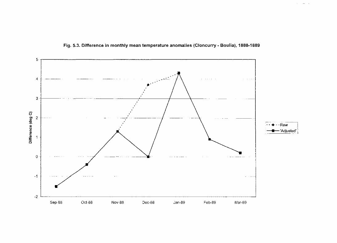
Fig. 5.3. Difference in monthly mean temperature anomalies (Cioncurry - Boulia), 1888-1889
5~--------------------------------------------------------------------------~
4 +-- ~ •
3
0 ~ 2
"C
I - I
I \ I Q) I --+--Raw
(,) I
c J( • 'Adjusted' Q) '-
~ 0
0
-1 +---~~-~ - -
-2~--------------------------------------------------------------------------~
Sep-88 Oct-88 Nov-88 Dec-88 Jan-89 Feb-89 Mar-89

Fig. 5.4. Cloncurry mean January maximum temperature predicted by multiple regression, using 1890· 1950 data
42~----------------------------------------------------------~
• • •
40 • ~~
C)
~ ~ . ~ . ~ . ~ .a ~,.--~ 36 - ~~.r . al --- • • ·--·. -~ -- . . -- . • ., -- --· . ., - ~ ,~~ . i3 34 4- • -~--- -- • ._ - • ... ~ •• • • • • •
• 32
,~~~'·
•
,'~-· --+
•
30~----------------------------------------------------------------------------------~
30 32 34 36 38 40 42 Predicted values (deg C)

value could be expected once in approximately 13,000 observations.
5.4. Daily temperatures at CJoncurry and Winton
Daily maximum and minimum temperatures were not readily available from Boulia for
the period of interest, but they were available from copies of original manuscript records
for Cloncurry and Winton for the period from November 1888 to January 1889. Fig. 5.5
shows the difference between the maximum temperatures at these sites over this period.
Over most of the three-month period, the 11-day running mean of the temperature
difference is ncar zero, but it exceeds 2°C in early December and mid-January.
Fig. 5.6 shows the frequency distribution of the difference between the daily tnaximum
temperatures of Winton and Cloncun·y during the period for which daily records are
available for both stations in the Bureau of Meteorology's digital database (1957-1975),
on days when the temperature at Winton exceeded 40°C. The mean annual number of
such days is 29. The greatest positive difference observed on such a day in this 19-year
period was 2.8°C. The 1888-89 summer contained 17 days with temperature differences
greater than this, reaching a peak of 8.6°C on December 6, 1888. On 16January 1889, the
maxin1u1n temperature at Winton was 49.0°C, 4.1 oc lower than that at Cloncurry.
5.5. Possible explanations for the anomalously high temperatures at Cloncurry in
the sununcr of 1888-89
The evidence presented above suggests that the maximum temperatures at Cloncurry
were unreasonably high during the summer of 1888-89, and in particular in early
December 1888 and mid-January, 1889.
115

The most likely cause of such a discrepancy is that the Cloncurry thermometer was
exposed to excessive solar radiation during this period. As noted previously, it is likely
that a non-Stevenson shelter was in use at Cloncurry at the time. If a Stevenson screen
had been in use at Boulia, it would be expected that anomalously high maximum
temperatures would have been recorded at Cloncurry (relative to Boulia) throughout
1888, but there is no evidence of any such anomalies prior to November. This, together
with the documentary evidence of Stevenson screens being installed at all three stations at
later dates, suggests that non-Stevenson screens were in use at both Cloncurry and Boulia,
and probably at Winton as well. As noted earlier in Chapter 3, this was common at many
Australian stations at this time.
In particular, the Glaisher stand was in common use in many parts of Australia until about
1910, particularly in South Australia and the Northern Territory (Nicholls et al., 1996b;
Torok, 1996), although other stands and instrument exposures apart from the Glaisher
stand were in widespread use in Queensland dming the 1880s (Nicholls et al. 1996b). The
Glaisher stand consisted of a vettical board, shaded from above, on which the
thermometers were mounted. It could be rotated to keep the instruments shielded from the
direct rays of the sun.
Stevenson screens progressively replaced other types of shelters through the period prior
to 1910. This process took place earlier in Queensland than in most other states (or
colonies as they were then), as the then Government Meteorologist, Clement Wragge,
was a keen proponent of the Stevenson screen (Parker, 1994).
Thermometers in a Glaisher stand were shielded from the direct rays of the sun, but were
still open to radiation from the ground, part of the sky and sun~ounding objects, and hence
higher mean maximum and lower mean minimum temperatures were recorded on them
than on those in a Stevenson screen, even when the stand was operated correctly (Laing
1977; Parker 1994). The difference in mean temperatures over 61 years of parallel
observations at Adelaide was approximately 0.2°C throughout the year for minima, and
ranged from 0.2°C in winter to 1.0°C in summer for maxima (Nicholls et al. 1996b).
116

0 C) (I)
~ (I) 0 c: (I) ... ~ 0
10
8
6
4
Fig. 5.5. Difference in daily maximum temperature (Cioncurry- Winton), November 1888 - January 1889
2~~--
0
-2
-4
-6
-8 > > 0 0 z z C0 0
> 0 z
;:::::
> 0 z ~ N
(.) Q)
e T"""
(.) Q)
0 co
(.) Q)
0 l?5
(.) Q)
0 C\l N
(.) Q)
0 05 N
c ro
"""')
l?5
c ro
"""')
C\l
c ro
"""')
05
c ro
"""')
(D N
--Difference I ---- - ·11-day running mean\

200
180
160
140
120 '-<» .c E 100 ::s z
80
60
40
20.
0
-7
Fig. 5.6. Frequency distribution of difference in daily maximum temperature (Cioncurry- Winton) on days exceeding 40 degress Cat Winton, 1957-1975
-6 -5 -4 -3 -2 -1 0 2
Difference (deg C)
3 4

Furthermore, if the stand was not rotated as required, the instruments could be exposed to
direct sunlight. In temperate latitudes this was most commonly a problem in the morning
and evening, but in the tropics the seasonal reversal of the direction of direct sunlight also
had to be taken into account. There have been no similar comparisons done over such
periods between the Stevenson screen and other types of shelters used in Australia, but it
is reasonable to believe that any change of instrument shelter may involve a bias in
recorded temperatures.
The sun is south of overhead at Cloncurry (latitude 20°43' S) at local noon for the
approximate period 28 November to 18 January, and at Winton (latitude 22°24' S) for the
period 6 December to 8 January. This makes the petiod frotn 8 to 18 January, during
which the record occuned, of particular interest, as the sun is south of overhead at
Cloncurry during this period, but not at Winton. If both stations were inconectly exposed
to the south, it would be expected that they would observe an01nalously high
temperatures for the periods when the sun was south of overhead, with the possible
exception of a few days at either end of the period when the sun was approximately
directly overhead at local noon. Hence, Cloncurry would be expected to be too warm
from late November or early December to mid-January, and Winton from mid-December
to early 1 anuary. It follows from this that the greatest temperature difference between the
sites would be expected in the period when the sun is south of Cloncurry but north of
Winton, in early December and mid-January, and that little difference between the two
would be expected when both are too hot, around the time of the summer solstice. This is
entirely consistent with the results observed in Fig. 5.5. If Winton was also incorrectly
exposed to the south, as the tninimal temperature differences in late December suggest, it
also brings into question the Winton observation of 50.6°C on 14 December 1888.
There arc a number of possible explanations for the thermometers being incorrectly
exposed to the south. As previously noted, the effectiveness of the Glaisher stand was
dependent on the conscientiousness of the observer in turning it to keep the thermometers
out of the sun's direct rays. Observers needed to be pat1icularly diligent at tropical sites,
where the sun is south of overhead (in the Southern Hemisphere) for a period dming
117

summer and the stand would therefore have to be turned in the opposite direction to that
in which it was turned for the rest of the year. If Glaisher stands were in use at the two
sites, it is possible that the stand was not turned at either site to take the reversed direction
of direct sunlight into account and that the thermometers were subject to direct solar
radiation in mid-summer, or to excessive radiant energy from the shelter structure. This
would also be the case if the thermometers were mounted on a south-facing wall, a
practice which Nicholls et al. (1996b) suggest was not unknown in Queensland at the
time. It is even possible that problems could arise in a Stevenson screen if the door is
facing south (as is the usual practice in Australia) and the door is left open for long
enough while observations are made for direct solar radiation to affect the instruments.
This has been noted as a problem in recent times (Bate, pers.comm.), but there is no
evidence of it causing discrepancies of the magnitude of those observed between
Cloncurry and Winton in 1888/89.
5.6. Implications for the Australian record high temperature
All known daily maximum temperatures in excess of 50°C in Australia arc listed in Table
5.1. Of these, the 1877 Bourke and the Mil dura and Eucla observations arc known to have
been taken using non-standard instrumentation (Crowder, 1995), and the Cloncurry and
Winton observations are discussed earlier in this chapter. The Oodnadatta, Wilcannia and
Mardie observations are known to have been taken in Stevenson screens. The Oodnadatta
observation is consistent with other observations throughout the region. Four other
stations exceeded 48°C on this day; Finke (48.3°C, a Northern Territory record), Port
Augusta (48.3°C), Whyalla (49.4°C) and Marree (49.4°C). Its authenticity is not in
serious doubt. The Wilcannia observation is also consistent with other observations in the
region (such as 49.7°C at Menindee and 47.8°C at Cobar), and took place dUting a period
of exceptionally high temperatures in south-eastern Australia, which saw records set at
many centres, including Adelaide, Melbourne and Sydney. The Mardie observation,
which occurred very recently, also took place during a period of general extreme heat in
the region, with record highs being set at Port Hedland (48.2°C), Roebourne (49.1 °C),
Pannawonica (48.2°C) and Onslow (48.0°C) either that day or the preceding day.
118

Table 5.1. Known daily maximum tentperatures of 50°C or greater in Australia
Temperature (°C) Station Month
53.1 Cloncurry January 1889
52.8* Bourke January 1877
51.9 Cloncurry December 1888
51.7 Bourke January 1 909
50.8* Mil dura January 1906
50.7* Eucla January 1906
50.7 Oodnadatta January 1 960
50.6** Winton December 1888
50.5 Mardi c. February 1998
50.0 Wilcannia January 1939
* Observations previously known to have been taken with non-standard instrumentation. ** The Winton observation has been cited as being higher in other sources, but these failed to take an index correction into account.

This leaves the Bourke observation of 3 January 1909 remaining for consideration. The
catalogue Climatological Stations: New South Wales (unpublished journal: lodged in the
National Meteorological Library at the Bureau of Meteorology) indicates that a Stevenson
screen was installed at Bourke in August 1908. However, no other station in New South
Wales or southern Queensland is known to have exceeded 47.2°C on this day.
The original manuscript record for Bourke shows temperatures of 125°F (51.7°C)
observed on both 2 and 3 January. The observation on 2 January has been corrected on
the manuscript to ll2°F (44.4°C), which is consistent with the temperatures over the
region, and with the 1500 temperature of ll0°F (43.3°C). The 3 January observation was
not corrected. However, 3 January was a Sunday, and no other observations were made
on this day (as was the usual practice at Bourke, and many other stations, at the time). It
is therefore likely that the observation is actually the tnaximum temperature for the 48
hours to 0900, 4 January, and therefore it would be affected by the same error which was
conected in the case of the 2 January observation. Reports from those stations in the
region which did take observations on both clays suggest that temperatures in the region
on 3 January were similar to those of 2 January.
Fig. 5.7 compares the temperature at Bourke with the mean of temperatures observed at
'rhargon1indah, Walgett and Coonamble on days when the daily maximum te1nperature at
Bourke exceeds 40°C during the periocll959-95. The mean difference is 0.5°C, and the
largest diflerencc observed during this 37-year period is 4.1 °C, while the difference on
January 3, 1909 was 6.9°C. This difference is sufficiently large to render the observation
suspect. As the screen and instrumentation are known to be standard, a possible cause of
any error would be clerical or observational. Nicholls et al. (l996b) note that many
Stevenson screens used at this ti1ne were in poor condition, and some had split wood on
top which allowed direct sunlight to enter the screen through the cracks, although the fact
that the screen was only a few months old makes this unlikely in the case of Bourke, and
the remainder of the month was not exceptionally hot compared with other stations in the
119

region. An observational error is more likely.
5.7. Conclusion
It is likely that the temperature presently recognised as the highest observed in Australia
was not recorded under conditions comparable with current standards. The most plausible
cause of the irregular observation appears to be a failure to adequately shelter the
instruments from incoming solar radiation during the period of the year when the sun is
south of overhead. If this was a widespread occurrence, it has potential implications for
the accuracy of climatic records throughout the tropics prior to the introduction of the
Stevenson screen.
The highest temperature in Australia known to have been taken under standard
conditions, and consistent with supporting observations from other sites, is 50.7°C,
recorded at Oodnadatta, South Australia, on 2 January 1960.
120

200
180
160
140
120 1-C1>
..c E 100 ::J z
80
60
40
20
0 -4
Fig. 5. 7. Frequency distribution of difference in daily maximum temperature (Bourke - (Walgett + Thargomindah + Coonamble)/3) on days exceeding 40 degrees Cat Bourke, 1959-1995
-3 -2 -1 0 2 3 4
Difference (degrees C)
5 6

Chapter 6
Models for the frequency distribution of daily maximum and
minimum temperatures
6.1. The data set for use in this study
The data set used in this chapter is a deseasonalised set of daily maximum and
minimUin stations, with quality control can·ied out as described in Chapters 3 and 4,
chosen fro111 the station network defined in Chapter 2.
The deseasonalisation for each station was can·ied out by computing a set of climate
means for each day of the calendar year (including February 29) for each station,
using the full period of record in each case. The means for each of these 366 days
were then smoothed using an unweighted 11-day running 1nean. The deseasonalised
series for each day was defined as:
Sy,m,d = 1~v.m,d- Nm,d
where Sy,n1,d is the deseasonalised daily maximum or tninimum (as appropriate)
temperature (henceforth referred to as a temperature anomaly), Ty, 1n,d is the observed
temperature and Nm,d is the smoothed mean temperature, for the d-th day of the m-th
month or year y.
The 1najor benefit of the use of deseasonalised data in the analysis of extremes is that,
in months in which the mean temperature changes substantially within a month, as
occurs in spring and autumn in southern Australia (and even more so in continental
regions of higher latitudes, in the event of such an analysis being extended to thetn),
data fron1 the stmt of a month can be considered, to some degree of approximation, as
being drawn from the same statistical population as that from the end of a month. This
approach does not take into account changes in the variance of daily tetnperature
between the start and end of a month, but the valiance shows a smaller annual cycle
than the mean at most stations (see Table 6.1).
121

An unpublished study canied out by the author compared the use of an 11-day
running mean to define daily temperature normals with six other methods, by
detennining the root-mean-square error in using normals derived for the 1961-90
period at a selection of 40 Australian stations as a predictor for daily temperatures in
1991-98. This found that six of the seven techniques tested (an 11-day running mean;
an 11-day binomial filter; the fitting of a cubic spline to the monthly means; the fitting
of three and five harmonics respectively to the monthly means; linear interpolation
from the monthly means) produced RMS errors differing by no more than 0.02°C,
with only the unsmoothed mean of daily temperatures performing substantially worse
than these. It follows that the selection of technique from within those tested to define
daily temperature normals makes little difference to the outcome.
6.2. Is the Gaussian distribution a satisfactory model for Australian daily
maximum and minimum temperatures?
6.2.1. The historical background
I-Iistorically, many studies of temperature have assumed, explicitly or implicitly, that
daily maximum and minimum temperatures follow the Gaussian (normal)
distribution. In particular, this assumption is implicit or explicit in n1any studies of
extreme or threshold temperature events, notably those of Mearns ct al. ( 1984) and
Katz and Brown (1992), although the former paper does acknowledge the possibility
of a non-Gaussian distribution without using it in any analysis. Kestin (2000), in her
study of Australian temperatures, used the Gaussian distribution whilst
acknowledging that it did not perform well at the extremes.
The source of this assumption is unclear; it appears periodically through publishing
history, but without any systematic global study to determine whether it is a realistic
assumption. Typical of the statements in the literature is that of Klein and Hammons
(1975), who assert that 'temperature is a continuous and nearly normally distributed
variable', whilst Thorn (1973) goes further, asserting (without any supporting
evidence) that studies finding a departure from the normal distribution were 'the result
of a lack of understanding of the statistical problem, i.e. that the data series must be a
122
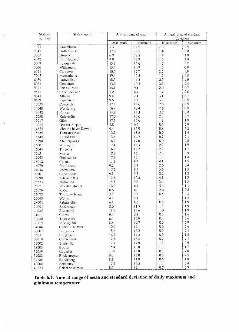
Station Station name Annual range of mean Annual range of standard number deviation
Maximum Minimum Maximum Minimum 1021 Kalumburu 5.3 11.2 1.3 2.9 2012 Halls Creek 12.0 12.5 1.4 2.0 3003 Broome 6.0 12.8 1.4 3.0 4032 Port Hetllantl 9.8 12.9 1.5 2.0 5007 Lcarmonth 13.8 12.6 !.7 1.2 5026 Wittenoom 15.7 14.9 1.2 0.9 6011 Carnarvon 10.5 12.7 2.1 1.9 7045 Meekatharra 19.4 17.3 1.5 0.8 8039 Dalwallinu 18.3 11.8 2.5 I .0 8051 Geraldton 13.0 10.2 3.5 0.4 9021 Perth Airport 14.1 9.1 2.9 0.7 9518 Cape Lccuwin 7.2 6.4 1.2 0.4 9741 Albany 9.4 7.1 3.1 0.7 9789 Esperance 9.6 7.5 3.3 0.9 10035 Cunderdin 17.7 11.6 2.6 0.9 10648 Wandering 16.9 10.4 2.6 0.8 11052 Forrest 14.9 11.3 2.7 0.9 12038 Kalgoorlic 17.0 13.6 2.3 0.7 13017 Giles 17.3 15.6 1.3 1.9 14015 Darwin Airport 2.8 6.0 0.3 0.9 14825 Victoria River Downs 9.4 13.9 0.8 3.2 15135 Tennant Creek 13.2 13.2 0.9 1.4
15548 Rabbit F1al 13.3 16.7 0.7 2.1
15590 Alice Springs 16.7 17.0 0.9 2.0 16001 Woomcra 17.4 13.3 2.7 1.9
16044 Tarcoola 16.9 13.2 2.7 1.1
17031 Marrec 18.2 16.1 2.3 0.9
17043 Oodnadaua 17.9 17.1 1.8 1.4
18012 Ceduna II. I 9.7 4.1 1.5 18070 Port Lincoln 9.2 7.8 2.6 0.4
21046 Snowtown 15.7 9.5 3.6 1.3
22801 Cape Borda 9.5 5.5 2.2 1.2
23090 Atlclaidc RO 13.5 10.2 4.3 1.3
23373 Nuriootpa 15.5 9.6 3.4 1.3 26021 Mount Gambier 12.0 6.4 4.4 1.1
26026 Robe 8.6 6.0 2.6 0.8
27022 Thursday Island 3.5 2.9 0.5 0.4
27045 Weipa 4.7 5.1 1.1 1.2
28004 Palmervillc 6.4 8.3 0.8 1.9
29004 Burketown 8.0 11.5 1.1 1.9
30045 Richmond 11.9 14.6 1.0 1.9
31011 Cairns 6.4 6.8 0.8 1.6
32040 Townsville 6.4 10.9 0.4 2.6
33119 Mackay MO 8.8 10.7 0.6 1.9
34084 Charters Towers 10.0 12.1 0.6 1.6
36007 Barcaldinc 13.3 15.2 0.9 2.1
36031 Longreach 14.2 16.2 0.9 1.8
37010 Camoowea1 12.3 15.4 0.7 2.1
38002 Birdsvillc 17.9 17.9 1.5 0.9
38003 Boulia 15.4 16.8 1.1 1.7
39039 Gayndah 10.7 13.8 0.7 2.0
39083 Rockhampton 9.0 13.0 0.8 2.5
39128 Bundabcrg 8.1 11.8 0.6 1.8
40004 Amberley 10.1 14.3 1.4 2.4
40223 Brisbane Airport 8.6 12.1 0.7 1.9
Table 6.1. Annual range of mean and standard deviation of daily 1naxitnum and minimum temperature

Station Station name Annual range of mean Annual range of standard number deviation
Maximum Minimum Maximum Minimum 40908 Tewantin 7.8 11.3 1.0 1.6 42023 Miles 13.6 16.4 1.1 2.4 43109 St. George 15.4 16.1 1.0 1.3 44021 Charleville 15.6 17.3 0.7 1.8 45017 Thargomindah 18.0 17.6 1.7 1.1 46037 Tibooburra 18.1 16.2 1.8 0.9 46043 Wilcannia 17.6 15.6 2.5 1.2 48027 Co bar 18.2 15.3 2.2 1.5 48239 Bourke 17.2 16.0 1.6 0.8 52088 Walgett 16.9 16.6 1.6 1.2 53048 Moree 16.3 15.9 1.6 1.6 55024 Gunnedah SC 15.6 13.9 1.7 0.8 56017 Inverell PO 14.3 15.5 1.0 1.2 58012 Yamba 7.7 10.9 1.0 0.9 59040 Coffs Harbour 8.2 12.2 1.4 1.5 60026 Port Macquarie 7.7 12.2 1.0 1.6 61078 Williamtown 10.7 11.9 2.6 1.0 61089 Scone SC 14.2 12.3 2.3 0.7 63005 Bathurst ARS 16.9 12.7 2.2 0.9 65012 Dubbo 17.7 15.1 1.8 1.1 66062 Sydney RO 8.9 10.7 1.8 0.6 67105 Richmond 12.5 13.5 2.8 1.9 68034 Jervis Bay 8.8 8.9 1.9 0.4 68076 Nowra 10.1 10.0 2.8 0.5 69018 Moruya Heads 7.8 10.7 1.7 0.9 70014 Canberra Airport I 6.4 13.4 2.8 1.4 72150 Wagga Wagga 18.7 13.4 2.6 1.1 72161 Cabramurra 16.7 11.5 1.7 1.9 73054 Wyalong 18.3 14.2 2.4 1.1 74128 Dcniliquin 17.5 12.5 2.8 1.6 76031 Mildura 17.3 11.8 2.<) 1.3 78031 Nhill I 5.9 9.4 3.5 1.6 80023 Kcrang 17.0 11.0 3.0 1.4 82039 Ruthcrglcn I 8.8 I l .4 2.6 1.0 84016 Gabo Island 7.8 8.0 1.3 0.6 84030 Orbost 10.6 9.0 3.3 0.8 85072 Sale 11.3 9.4 3.0 0.6 85096 Wilsons Promontory 8.4 6.4 3.0 0.8 86071 Melbourne 12.5 8.6 4.1 0.5 87031 La vert on 12.7 8.9 4.2 1.0 90015 Cape Otway 8.5 6.7 3.3 1.0 91057 Low Head 9.9 7.7 1.0 1.0 91104 Launccston Airport 12.3 7.8 1.9 0.7 92045 Eddystone Point 7.8 7.4 [.[ 1.2 94010 Cape Bruny 7.7 6.4 2.2 0.5 94029 Hobart RO 10.0 7.6 2.2 0.6 94069 Grove 10.6 7.5 2.5 0.6 96003 Butlers Gorge 11.6 6.7 3.3 0.7
Table 6.1 (cont.). Annual range of mean and standard deviation of daily maximum and minimum temperature

climatological series', where he defines a climatological series as 'a homogeneous
series of values of the predictand variable, one value taken from each year'. The
WMO Guide to Climatological Practices (1983) also suggests a hearly normal'
distribution for daily maximum and minimum temperatures. The assumption may be
founded on the climates of western Europe and the eastern United States. A number of
local studies (e.g. Bruhn et al., 1980) have found that daily temperatures in specific
regions and seasons are approximately nonnally distributed.
As the methodology of Katz and Brown forms a substantial part of the theoretical
foundations of this thesis, the assumption needs to be evaluated for its validity under
Australian conditions.
6.2.2. Results of a study of the Australian data set
The question of whether the data are normally distributed is of more than trivial
consequence for the expected frequency of extreme temperature events. Table 6.2
shows the frequency of daily maximum and 1ninimum temperature anomalies
departing from the mean by more than 3 standard deviations (defined as extreme
events in this section), using the standard deviation derived for each calendar month.
In a normal distribution, the expected frequency of such events is 0.27%.
The results shown in Table 6.3 show that the assumption of a Gaussian distribution
for Australian data would result in a highly misleading estimate of the frequency of
extremes in many cases. The median frequency of maximum temperature anomalies
of this magnitude across the 103-station network ranges from 0.47o/c) in spring to
0.57% in autumn, approximately double the expected value in a normal distribution.
In contrast, winter minimum temperature anomalies of this size occur with less than
half the expected frequency, with a value of 0.12o/o, although departures in other
seasons are less prominent. As a further indicator of the extent to which the normal
distribution fails to represent the expected frequency of extretnes, 39 of the 103
stations have extreme event frequencies below 0.07% (one-quarter of the expected
value) for winter minima, whilst for maxima, 28 stations have frequencies exceeding
1.08% (four times the expected value) in summer, and 21 in spting. High frequencies
of extreme maxima are particularly pronounced in coastal locations, whilst low
123

frequencies of extreme minima in winter are most pronounced in Queensland (other
than the far north and west) and inland New South Wales.
6.2.2.1. Assessment of the normality of Australian daily temperature data
Five tests were carried out to detect departures of a frequency distribution from a
normal (Gaussian) distribution of unspecified mean and variance, applied to
Australian daily maximum and minimum temperature anomaly data. The tests used
are those of Kolmogorov-Smimov (D), Kuiper (V), Cramer-von Mises (W2), Watson
(U2), and Anderson-Darling (A).
Full details of the tests are given in Appendix A. According to Stephens (1970) and
Pearson and Hmiley (1976), in the tails of a distribution- an area of particular interest
in this study - A, followed by W 2, is the most powerful of the tests for detecting
deviations. The chi-square test, used in some literature (e.g. Grace et al., 1991), has
the limitations that the values it generates are dependent upon the (arbitrary) choice of
the width of the class interval used in the test, introducing an element of subjectivity,
and that it is extremely sensitive to a small number of outliers, irrespective of the
goodness-of-fit of the remainder of the distribution (although this is not necessmily a
disadvantage if the modelling of extreme outliers is the highest priority).
A full listing of the outcome of the tests is given in Appendix C (Tables C.l and C.2).
The frequency distribution of daily temperature anomalies, in an examination of the
I 03 stations for the 12 calendar months (1236 station-months in total), was found to
differ from the normal distribution at the 99% level in all five tests:
-In 86% of station-months for maximum temperature
-In 81 o/o of station-months for minimum temperature
124

Station Name Summer Autumn Winter Spring number Min Max Min Max Min Max Min Max 39083 Rockhampton 0.33 0.50 0.79 0.80 0.00 0.78 0.46 0.48 39128 Bunda berg 0.17 1.37 0.49 0.87 0.00 0.66 0.08 1.11 40004 Amberley 0.22 0.50 0.12 0.98 0.00 0.63 0.04 0.53 40223 Brisbane AP 0.12 1.10 0.65 1.16 0.00 1.02 0.34 1.37 40908 Tewantin 0.35 1.56 0.83 1.18 0.00 0.97 0.22 0.75 42023 Miles 0.64 0.47 0.31 0.62 0.00 0.13 0.09 0.44 43109 St. George 0.16 0.87 0.03 0.57 0.03 0.06 0.03 0.16 44021 Charlcville 0.19 0.77 0.28 0.46 0.00 0.06 0.02 0.18 45017 Thargomindah 0.21 0.55 0.06 0.17 0.35 0.11 0.03 0.08 46037 Tibooburra 0.14 0.26 0.14 0.15 0.45 0.18 0.14 0.08 46043 Wilcannia 0.24 0.23 0.15 0.09 0.21 0.38 0.38 0.06 48027 Co bar 0.16 0.36 0.00 0.14 0.22 0.41 0.16 0.05 48239 Bourke 0.08 0.45 0.08 0.22 0.28 0.41 0.11 0.03 52088 Walgett 0.32 0.64 0.09 0.48 0.23 0.09 0.18 0.06 53048 Moree 0.47 0.56 0.27 0.64 0.05 0.21 0.04 0.23 55024 Gunncdah SC 0.31 0.31 0.24 0.61 0.07 0.20 0.32 0.17 56017 Invcrell PO 0.11 0.31 0.08 0.83 0.14 0.25 0.03 0.25 58012 Yamba 0.56 1.39 0.19 1.03 0.23 0.83 0.21 1.81 59040 Coffs Harbour 0.29 1.18 0.43 0.93 0.05 0.90 0.21 1.30 60026 Port Macquaric 0.19 0.97 0.13 0.85 0.09 0. 70 0.10 1.35 61078 Williamtown 0.26 0.62 0.02 0.71 0.09 0.75 0.07 0.60 (J]089 Scone SC 0.28 0.07 0.14 0.10 0.07 0.24 0.31 0.10 63005 Bathurst J\RS 0.16 0.10 0.04 0.26 0.04 0.16 0.22 0.12 (J5012 Dubbo 0.33 0.22 0.03 0.38 0.03 0.16 0.11 0.22 66062 Sydney RO 0.39 1.56 0.33 0.79 0.50 0.61 0.39 0.99 67105 Richmond 0.38 0.12 0.15 0.54 0.09 0.77 0.09 0.19 68034 Jervis Bay 0.62 1.21 0.35 0.61 0.58 0.57 0.49 1.07 (>8076 Nowra 0.08 1.19 0.21 0.53 0.22 0.70 0.38 0.89 69018 Moruya Heads 0.41 2.37 0.35 1.13 0.45 0.89 0.25 2.13 70014 Canberra Airport 0.21 0.06 0.07 0.45 0.00 0.49 0.11 0.27 72161 Cabramurra 0.00 0.41 0.06 0.50 0.34 0.25 0.22 0.06 72150 Wagga Wagga 0.24 0.20 0.00 0.12 0.06 0.36 0.14 0.40 73054 Wyalong 0.21 0.32 0.10 0.09 0.17 0.34 0.17 0.22 74128 Dcniliquin 0.28 0.03 0.03 0.11 0.03 0.60 0.19 0.47 7(103 I Mildura 0.2(l 0.04 0.13 0.09 0.15 0.48 0.37 0.43 7X031 Nhill 0.31 0.06 0.00 0.19 0.16 1.12 0.1 () 0.63 80023 Kerang 0.17 0.00 0.21 0.20 0.21 0.91 0.21 0.38 82039 Ruthcrglen 0.10 0.28 0.10 0.07 0.00 0.48 0.18 0.42 84016 Ciabo Island 0.29 1.29 0.31 0.82 0.25 0.98 0.45 1.90 84030 Or host 0.20 0.45 0.08 0.22 0.14 0.42 0.25 0.43 85072 Sale 0.04 0.69 0.09 0.66 0.22 0.87 0.15 1.12 85096 Wilsons Prom. 1.13 2.19 0.66 1.29 1.06 1.28 1.27 1.82 8(1071 Melbourne RO 0.80 0.08 0.21 0.27 0.05 0.38 0.58 0.32 87031 Laverton 0.64 0.10 0.02 0.23 0.06 0.71 0.37 0.66 90015 Cape Otway 0.99 1.88 0.62 1.29 0.42 1.02 1.14 1.31 91057 Low Head 0.50 0.30 0.08 0.14 0.00 0. 1 1 0.06 0.47 91104 Launceston AP 0.04 0.73 0.00 0.29 0.00 0.44 0.02 0.58 92045 Eddystone Point 0.33 1.41 0.03 0.54 0.06 0.63 0.21 1.28 94010 Cape Bruny 0.72 1.64 0.49 0.94 0.28 0.41 0.54 1.39 94029 Hobart RO 0.60 1.27 0.18 0.56 0.21 0.18 0.39 1.04 94069 Grove 0.30 0.95 0.16 0.36 0.30 0.22 0.14 0.95 96003 Butlers Gorge 0.29 0.00 0.12 0.06 0.12 0.15 0.25 0.21
Table 6.2 (cont). Percentage frequency of n1aximum and minimum temperatures more than 3 standard deviations front ntean

Station Name Summer Autumn Winter Spring number Min Max Min Max Min Max Min Max 1021 Kalumburu 0.20 0.40 0.68 0.98 0.06 0.49 0.69 0.72 2012 Halls Creek 0.70 0.73 0.79 1.13 0.25 0.51 0.51 0.80 3003 Broome 0.56 1.58 0.23 0.82 0.00 0.44 0.45 0.47 4032 Port Hedland 0.51 0.19 0.18 0.90 0.02 0.65 0.41 0.02 5007 Learmonth 0.15 0.15 0.45 0.35 0.10 0.39 0.70 0.15 5026 Wittenoom 0.12 1.32 0.29 1.01 0.14 0.54 0.14 0.65 6011 Carnarvon 0.69 1.24 0.11 0.27 0.09 0.64 0.13 1.30 7045 Meekatharra 0.24 0.78 0.16 0.26 0.12 0.09 0.21 0.12 8039 Dalwallinu 0.17 0.17 0.20 0.08 0.03 0.42 0.37 0.17 8051 Gerald ton 0.24 0.06 0.14 0.12 0.06 0.74 0.20 0.87 9021 Perth Airport 0.27 0.02 0.13 0.17 0.00 0.70 0.17 0.91 9518 Cape Leeuwin 0.71 2.26 0.44 1.29 0.46 0.60 0.45 1.21 9741 Albany 0.15 1.34 0.15 0.82 0.23 0.44 0.09 1.31 9789 Esperance 0.28 0.91 0.27 0.54 0.38 0.57 0.39 1.21 10035 Cunderdin 0.28 0.19 0.11 0.14 0.22 0.61 0.20 0.34 10648 Wandering 0.31 0.09 0.03 0.11 0.00 0.39 0.06 0.36 11052 Forrest 1.05 0.02 0.72 0.13 0.47 0.52 0.90 0.00 12038 Kalgoorlie 0.16 0.30 0.22 0.02 0.20 0.33 0.20 0.06 13017 Giles 0.30 1.18 0.33 0.84 0.41 0.08 0.11 0.51 14015 Darwin AP 0.08 0.74 0.70 1.15 0.29 0.45 0.59 0.73 14825 Viet. R. Downs 0.68 0.47 0.43 0.70 0.00 0.20 0.21 1.50 15135 Tennant Creek 0.42 0.70 0.49 0.93 0.05 0.19 0.25 0.94 15548 Rabbit Flat 0.33 0.59 0.12 1.39 0.00 0.29 0.08 0.98 15590 Alice Springs 0.06 1.10 0.10 0.34 0.26 0.04 0.10 0.32 16001 Woomera 0.28 0.32 0.12 0.11 0.20 0.39 0.19 0.18 16044 Tarcoola 0.17 0.13 0.16 0.16 0.16 0.47 0.48 0.06 17031 Marree 0.08 0.31 0.08 0.11 0.33 0.59 0.20 0.11 17043 Oodnadatta 0.05 0.46 0.11 0.21 0.29 0.75 0.09 0.11 18012 Ceduna 0.36 0.02 0.14 0.24 0.08 0.82 0.18 0.18 18070 Port Lincoln 0.45 1.74 0.27 1.45 0.44 1.01 0.25 1.57 21046 Snowtown 0.33 0.00 0.15 0.06 0.18 0.59 0.42 0.12 22801 Cape Borda 1.88 0.32 0.72 0.50 0.23 0.53 0.91 0.87 23090 Adelaide RO 0.73 0.00 0.50 0.15 0.13 0.81 0.67 0.25 23373 Nuriootpa 0.19 0.00 0.25 0.11 0.05 0.87 0.36 0.08 26021 Mount Gambier 0.63 0.24 0.28 0.57 0.10 0.79 0.46 0.74 26026 Robe 0.68 1.14 0.25 0.74 0.24 0.42 0.12 0.77 27022 Thursday Island 0.26 0.44 0.31 0.52 0.56 0.85 0.31 0.91 27045 Weipa 1.18 0.48 0.81 1.16 0.65 0.91 0.76 0.37 28004 Palmerville 0.79 1.07 0.57 1.24 0.73 0.83 0.91 0.68 29004 Burketown 0.36 0.35 0.52 1.03 0.17 0.49 0.52 0.61 30045 Richmond 0.67 0.97 0.26 1.25 0.03 0.29 0.24 1.07 31011 Cairns 0.55 1.44 0.93 0.87 0.50 0.54 0.51 1.24 32040 Townsville 0.41 1.41 0.37 1.44 0.10 1.09 0.43 1.52 33119 Mackay MO 0.27 0.65 0.51 0.83 0.00 0.89 0.20 0.44 34084 Charters Towers 0.32 0.74 0.42 0.95 0.03 0.59 0.16 0.84 36007 Barcaldine 0.29 1.04 0.32 1.01 0.00 0.25 0.35 0.42 36031 Longreach 0.30 1.32 0.29 1.20 0.00 0.16 0.00 0.47 37010 Camooweal 0.47 0.61 0.12 1.16 0.03 0.28 0.20 1.08 38002 Boulia 0.19 1.11 0.45 1.01 0.12 0.14 0.16 0.42 38003 Birds ville 0.14 0.79 0.06 0.31 0.45 0.23 0.14 0.06 39039 Gayndah 0.14 0.64 0.14 0.79 0.05 0.52 0.22 0.47 Table 6.2. Percentage frequency of maximum and minimum temperatures more than 3 standard deviations from mean
The expected frequency of such events in a normal distribution is 0.27%. Values exceeding this in the table have been shown in bold type.

Summer Autumn Winter Min Max Min Max Min Max Min
Number of stations with 59 74 41 67 24 74 39 frequency: > 0.27(/tJ < 0.07% 5 13 15 3 39 3 10 > 1.08% 3 28 0 26 0 3 2 Median frequency(%) 0.29 0.55 0.19 0.57 0.12 0.48 0.21
Table 6.3. Summary statistics for frequencies of temperature anon1alies exceeding 3 standard deviations
Notes:
• There are 103 stations in total.
Spring Max 71
10 21 0.47
• 0.07% and 1.08% arc approximately 14 and 4 times, respectively, the expected frequency (in a normal distribution) of 0.27%.

At least one of the five tests showed a departure from the normal distribution at the
95% level:
-In 95% of station-months for maximum temperature
-In 94% of station-months for minimum temperature
These figures are clearly far above those which would be expected by chance, and
indicate that it cannot be validly assumed that Australian daily maximum and
minimum temperature data are normally distributed.
6.2.2.2. The nature of the departures from norn1ality
Figs. 6.1 and 6.2 show the skewness over Australia for maximum and minimum
te1nperature anomalies respectively for sample months in each season. The full listing
of skewness values is given in Table C.7.
Table 6.4 shows that the skewness of the distribution differs significantly from 0 at
the 5o/a level for 84~) of station-months for maximUin temperature, and 70% for
minimum temperature. Differences significant at the 1% level occur for 80~; of
station-months for maximum temperature and 60% for minimum temperature. This
degree of skewness is comtnon to all seasons.
As a very broad generalisation, maximum temperature tends to be positively skewed
in southern mainland Australia, and negatively skewed in northern Australia. The
boundary between the two regions displays considerable seasonal variation. In
summer and autumn, positively skewed distributions are found in the in1mediate
vicinity of the western coast (except for the Pilbara coast in autumn), and the eastern
coast south of Fraser Island, as well as in a broader region within about 500
kilometres of the southern coast, and throughout Tasmania. The greatest positive skew
occurs at sites highly exposed to coastal influences, such as Cape Leeuwin, Cape
Otway, Wilsons Promontory and Moruya Heads, where the maximum temperature
regime is dominated by maritime influences, but where temperatures occasionally rise
to very high levels when strong offshore winds occur. The strongest negative skew in
summer is found over a broad region of western and central inland Australia centred
125

h f. '1()0 S These arc rcgi ( •n on latitude 25os, whilst in autumn it occurs nort o .;.. . , . .
. . d/ 1 dy days result in maximum temperatures \\'ell hclrJ\\ occasional ramy an or c ou
which occur during the (more usual) clear conditions.
. h k (both negative and positive) of the distrihuti on t<.~nd' h In wmter, t e s ewness
lower (only one station has skewness outside the runge -1.0 to 1.0 in July. t..·e
with 20 in January), and positive skew is found much further north, occurnng tn
of the region south of the Tropic of Capricorn, except in the vicinitY of tht" C
Dividing Range in New South Wales and southern Queensland. (This is illu"t
the occurrence of positive skew for 76% for station-months in spring and !*'·~"
winter (Table 6.4), compared with 41% in summer). The marked increase in sJ ... t~w
towards the western and southern coast which occurs in summer is als< > largl'"l Y
in winter. In spring, positive skew is found in similar areas to those in \\·inter. hut
magnitude of skewness is greater, particularly ncar the southern coast and Ul
northern inland.
The pattern of skewness of minimum temperature is more complex, \vith de
skewness generally lower than for maximum temperature, as suggested bv
frequency of significant departures from 0 described above, and rnarkc.:d sc~ts.t
variations in the spatial distribution of skewness. In spring and surn r ncr. [H ,~, lll\
skewed distributions occur in similar regions of southern Australia to t h u "'c \\
they occur for maxima (but not on the eastern and western coasts, except for rhe \a.t."~~~
in spring). Weak negative skew occurs over much or the rest of the country. hur u h
only locally significant. Autumn and winter show a markedly di rrercnt path,*rfl
Significantly positively skewed distributions occur in winter over a hn lad
between 20o and 30°S, with the strongest skewness in in land southern () ueens 1 and and
northern New South Wales, whilst the largest regions with negative skew an.: on
near the coasts of south-western Western Australia, South Australia and Victona. ~~s well as those of north Queensland and the Northern TeiTitory. Conversely, in uutunln
significant positively skewed distributions are largely confined to Victoria and Suuth
Australia, with negative skew being most prominent in northern Australi u and neur the Queensland coast.
A model of a skewed, unimodal distribution, as used by authors such as Horton et at
126

January , t;J
~
Cjti
10.0
2.0
1.0
0.5
0.0 -0.5
-1.0
-2.0
-10.0
10.0 2.0
1.0
0.5
0.0
-0.5
-1.0
-2.0 -10.0
Fig. 6.1. Skewness of daily maximum temperature
I
October '
~~-~ ' . ~~
~~ ~;f ·~
10.0
2.0
1.0 0.5
0.0
-0.5
-1.0
-2.0
-10.0
10.0
2.0
1.0
0.5
0.0
-0.5
-i .0
-2.0 -10.0

January ~
0
\j
,! I
tJ
10.0
2.0
1.0
0.5
0.0
-0.5
-1.0
-2.0
-10.0
10.0
2.0
1.0
0.5
0.0
-0.5
-1.0
-2.0 -10.0
Fig. 6.2. Skewness of daily minimum temperatures
~ \
\e
D a
October l
~ v
10.0
2.0
1.0
0.5
0.0
-0.5
-1.0
-2.0
-10.0
10.0
2.0
1.0
0.5
0.0
-0.5
-1.0
-2.0 -10.0

Skewness Maximum ((JfJ of station-months) Minimum (%of station-months) Sum Aut Win Spr Tot Sum Aut Win Spr Tot
Negative - significant at 999~J 48 40 24 18 32 30 29 20 27 27 level Negative - significant at 95% 4 3 2 1 3 5 5 4 4 4 level Negative- not significant 7 8 10 5 7 17 17 14 10 15 Total negatively skewed 59 50 36 24 42 52 51 38 41 46 Positive - significant at 99(XJ 32 40 53 63 47 29 30 37 40 34 level Positive - significant at 95% 3 2 1 3 2 4 4 7 6 5 level Positive- not significant 6 8 10 10 9 15 15 17 13 15 Total positively skewed 41 50 64 76 58 48 49 62 59 54 Total skewed at 99% level of 80 80 77 81 80 59 59 57 67 60 significance Total skewed at 95% level of 87 84 80 85 84 68 68 69 77 70 significance
Table 6.4. Station-months with positive and negative skewness of daily ten1perature
l. The seasons are defined as summer ( 1 December - 29 February), autumn ( 1 March- 31 May), winter ( 1 June- 31 August), and spring ( 1 September- 30 November). 2. Totals may not add due to rounding.

(200 1 ), is also an incomplete description of the frequency distribution of daily
temperature within Australia. Two interesting local examples of frequency
distributions which are broadly symmetric, but nevertheless depart significantly from
the normal distribution, illustrate this, with sample distributions shown in Figs. 6.3a
and 6.3b. In mid-winter, the frequency distribution of minimum temperature in much
of inland southern New South Wales generally shows small (and non-significant)
positively skewness, but displays no clear mode, with peak frequencies distributed
fairly uniformly over a range of several degrees Celsius. This manifests itself in
values of kurtosis widely in the 2-2.5 range, well below the value of 3 expected in a
normal distribution. Conversely, on parts of the coast of northern Queensland in
summer, the tendencies to marked negative outliers in the tropical inland, and to
positive outliers on the coasts, coincide to produce a distribution with relatively high
frequencies of extreme anomalies, both positive and negative.
6.3. Alternative models for the frequency distribution of Australian daily
maxirnum and minimum temperatures
6.3.1. The gamn1a distribution
The 3-paramcter gamma distribution has been used in recent work, notably Horton et
a!. (200 1 ), as a model for the frequency distribution of tnean temperatures on the
daily, n1onthly and annual timescale. This follows initial work by Lehman (1987),
who used a 2-parameter gamma distribution to describe the frequency distribution of
daily tnean temperatures. In effect, this is based on a 2-parameter gmnma distribution
(which, by definition, tnust be positively skewed and is bounded below by 0), with a
third parameter allowing location, scale and sign transformations possible to allow for
positive and negative values of the variable, and possible negatively skewed
distributions. It is a unimodal disttibution.
The 2-parameter gamma distribution is defined as:
127

where x is the variable being studied, a and b are parameters which describe the
distribution, and T(a) = (a-1 )I is the gamma function.
This distribution is defined only for x~O. In order to use this distribution to model a
temperature frequency distribution which is, for all practical purposes, unbounded
above and below, it is necessary to transform the data using a third parameter, c, and
the transformation:
x. -x z. =c+g-'-
I S
where x and s are the sample mean and standard deviation respectively of the data
points xi, and g takes the value 1 if the data are positively skewed, or -1 is it is
negatively skewed.
6.3.2. The compound Gaussian distribution
The first known use of this distribution to model the frequency distributions of
Australian daily maximum and minimum temperature was by Grace ct al. (1991),
with further development by Grace and Curran (1993). It has also been used
elsewhere by Bryson (1966) and Colman (1986) for daily maximum and minimum
temperature, by Marchcnko and Minakova (1980) for hourly air temperature, and by
Essenwanger ( 1954, 1955) for monthly precipitation. Grace and Cunan refer to the
distribution as the 'binormal' distribution, but this term has also been used to refer to
other distributions (e.g. Toth and Szentimrey, 1990) and implies a mixture of only two
distributions. For these reasons the term 'compound Gaussian' is used in this thesis.
The model used in this thesis is defined by the equation:
k
f (X) = 2: w k N (j.i k ' (]' k ) ' I
128

Fig. 6.3a. Frequency distribution of June minimum temperature, Canberra
0.0045~----------------------------------------------------------------------~
0.004 +------------------------------------------------------------------------------; ~·- ......... ,
0.0035 \
0.003 I
0.0025 +- '.------'.....__~~~-
--Observed 1 • - - • • -Gaussian distribution
0.002 -t--- -------- --------1- . -.---\------·--·-----------------------------!
0.0015
0.001 +-------- --------
0.0005 +-----------
0 •....•
-15 -10 -5 0 5 10 15 20
Temperature (deg C)

Fig. 6.3b. Frequency distribution of January maximum temperature, Cairns
0.006~--------------------------------------------------------------------~
0.005 +-------------------------1-~--------------1
0.004+-----------------------------------------~----~----------------------~
0.003 -t ---1
0.002 -t~~----~--~~----~--~---- -----~'---+-----------\--':-------------1
0.001
0 •. -- --
20 25 30
Temperature (deg C)
35 40
!--Observed · - - - - - · Gaussian distribution
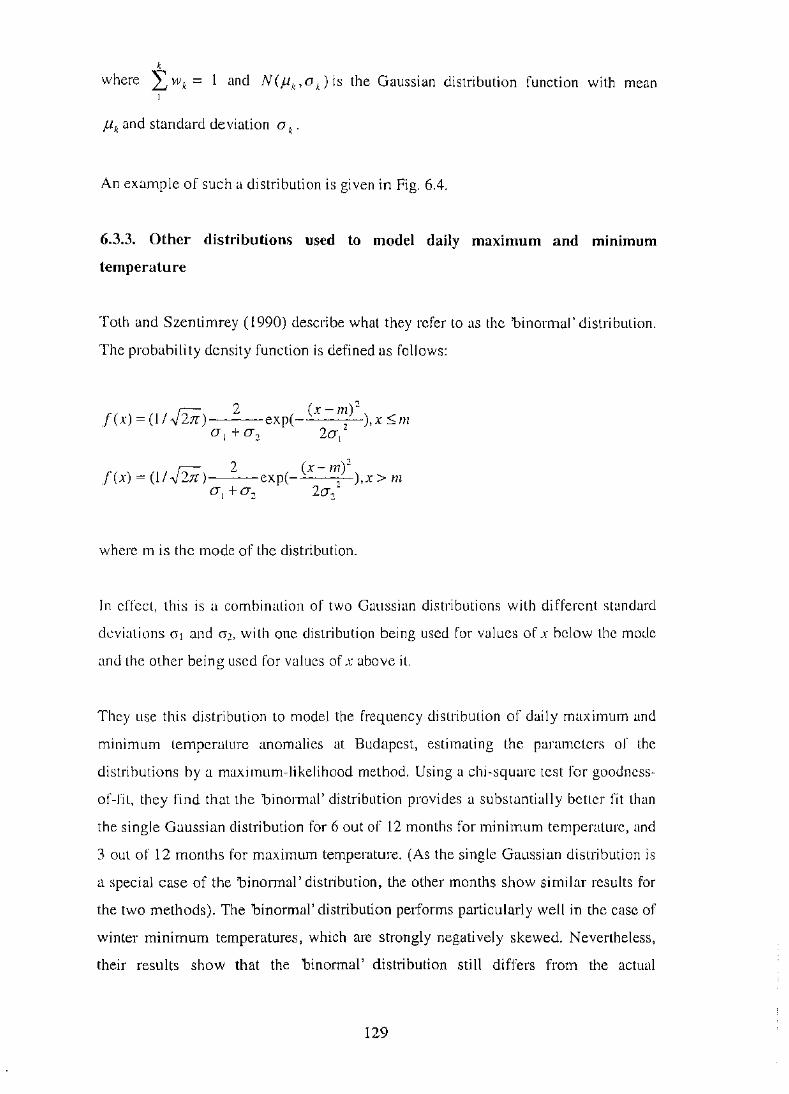
k
where L, wk = 1 and N(JLk ,o k) is the Gaussian distribution function with mean
Jlk and standard deviation o k.
An example of such a distribution is given in Fig. 6.4.
6.3.3. Other distributions used to model daily maximum and minimum
temperature
Toth and Szentimrey ( 1990) describe what they refer to as the binormal' distribution.
The probability density function is defined as follows:
f. r;:::-:: 2 (x- m) 2
. (x)=(ll\f2n) exp(-2
),x~m a- I + O"z 2a!
where m is the mode of the distribution.
In effect, this is a combination of two Gaussian distributions with different standard
deviations a 1 and cr2, with one distribution being used for values of x below the mode
and the other being used for values of x above it.
They use this distribution to model the frequency distribution of daily maxiinum and
minimum temperature anomalies at Budapest, estimating the parameters of the
distributions by a maximum-likelihood method. Using a chi-square test for goodness
of-fit, they find that the binormal' distribution provides a substantially better fit than
the single Gaussian distribution for 6 out of 12 months for tninimum temperature, and
3 out of 12 months for maximum temperature. (As the single Gaussian distribution is
a special case of the binormal' distribution, the other months show similar results for
the two methods). The binormal' distribution petforms particularly well in the case of
winter minimum temperatures, which are strongly negatively skewed. Nevet1heless,
their results show that the binormal' distribution still differs from the actual
129

distribution at the 5% level in 6 months for minimum temperature, and 3 months for
maximum temperature.
6.4. An evaluation of the three-parameter gamma and compound Gaussian
distributions
6.4.1. Methods of fitting distributions to empirical data
6.4.1.1. The gamma distribution
The procedure used by Horton et al. (2001) was used. This involved, m the first
instance, defining q as follows:
- where the data are positively skewed:
- where the data are negatively skewed:
c = q +I min (x) I c = q + I max ( x) I
where min(x) and max(x) are the lowest and highest values of the series x and c is a
parameter of the gamma distribution as defined in section 6.3.1 i· This definition
ensures that, for positive q, the Zi are also positive, as required in order to fit the
definition of the gamma distribution.
The best-fit value of q was determined by a process of iteration. The first-guess value
of q was taken as 0.5. The maximum-likelihood method was used to calculate a:
a =(I t~l t4A/3) I 4A
- 1 with A=lnx--2:lnxi, whereNisthesample size.
N
-Using the relationship ab = x, b was then estimated and the skewness of the
distribution (which is equal to 2a-112) was calculated.
130

0.0045
0.004
0.0035
0.003
0.0025
0.002
0.0015
0.001
0.0005
0
-5 -4 -3
Fig. 6.4. Example of the compound Gaussian distribution
-2 -1 0 2 3
z
4 5
1- --- Component 1
'-----·Component 2
---Overall distribution

The value of q was then raised by 0.5 and the process repeated. This was continued
until the difference between the observed and fitted skewness reached a minimum- in
which case the value of q giving the closest fit to the skewness was used - or a
exceeded 50.
6.4.1.2. The compound Gaussian distribution
A number of procedures have been used in previous work. Grace et al. (1991) used an
iterative process on the unknowns (of which there were five, as they were constrained
to two subdistributions), with the aim of optimising the goodness-of-fit as determined
by the chi-squared statistic. Colman (1986) used the assumption that the two tails of
the overall frequency distribution were each generated entirely from one of the sub
distributions, and used this to estimate the parameters of those sub-distributions (and,
by means of examining the residuals, any additional sub-distributions). Marchenko
and Minakova (1980) used a moments-based method.
The method used in this study was based on the method of 1-Iasselblad (1966). This
involves finding, iteratively, maxixnum likelihood estimates for the parameters of the
sub-distributions. The procedure can be explained as follows:
131

Let there be K sub-distributions, and define Wk,r, uk,t and sk,t as the t-th iteration of the
estimates of the weighting, mean and standard deviation of the k-th sub-distribution.
Let there be a total of N observations, XJ, x2, ... , XN in the distribution being modelled
(which, in this case, is the set of all observations of maximum or minimum
temperature at a station for a given month of the year). Fut1hermore, let fk.i be the
probability that an observation Xi will lie in the k-th sub-distribution, assuming that the
distribution is the mixture of Gaussian sub-distributions with the estimated parameters
wk,~> Uk,t and Sk,r. For iteration (t+ 1) we then have:
N
'Li~.i i=l
wk,t+l = N
N
Lfk.ixk,i i=l
ukt+I =----, Nwk,t+I
Initially, this system of equations was evaluated for K=2, and with the initial
estimates:
W 1,1 = W2.1 = 0.5
U1,1 = -0.5
U2,1 = 0.5
SJ,J = S2,1 = 0.6
The iteration was carried out until the following convergence criteria were satisfied
for all k:
I (wk,(t+lJ- wk,r) I < 0.005
I (uk,(t+l)- uk,r) J < 0.001
I (Sk,(t+l)- Sk,t) I < 0.001
132
!1'-
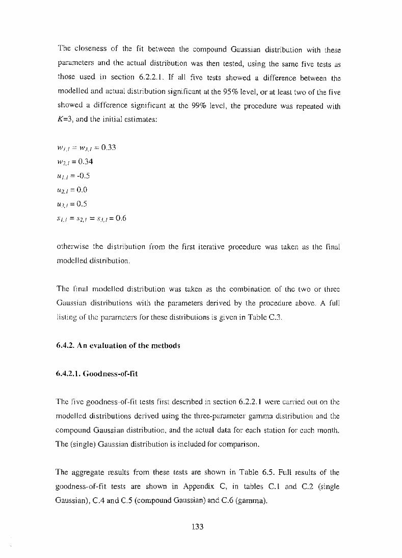
The closeness of the fit between the compound Gaussian distribution with these
parameters and the actual distribution was then tested, using the same five tests as
those used in section 6.2.2.1. If all five tests showed a difference between the
modelled and actual distribution significant at the 95o/o level, or at least two of the five
showed a difference significant at the 99% level, the procedure was repeated with
K=3, and the initial estimates:
w /,I = w.u = 0.33
w2,1 = 0.34
UJ,J = -0.5
u2,1 = 0.0
UJ,I = 0.5
SJ,/ = S2,/ = 83,1 = 0.6
otherwise the distribution from the first iterative procedure was taken as the final
modelled distribution.
The final modelled distribution was taken as the c01nbination of the two or three
Gaussian distributions with the parameters derived by the procedure above. A full
listing of the pararneters for these distributions is given in Table C.3.
6.4.2. An evaluation of the n1ethods
6.4.2.1. Goodness-of-fit
The five goodness-of-fit tests first described in section 6.2.2.1 were carried out on the
modelled distributions derived using the three-parameter gamma distribution and the
compound Gaussian distribution, and the actual data for each station for each month.
The (single) Gaussian distribution is included for cotnparison.
The aggregate results from these tests are shown in Table 6.5. Full results of the
goodness-of-fit tests are shown in Appendix C, in tables C.l and C.2 (single
Gaussian), C.4 and C.5 (compound Gaussian) and C.6 (gamma).
133

It is apparent from these results that the compound Gaussian distribution is by fisr
most effective model for the simulation of the full frequency distribution of
daily maximum and minimum temperatures. The three-parameter garn n1 a d t stn
is a substantial improvement on the single Gaussian distribution. hut it stt1l fit,
actual distribution less well than the compound Gaussian distribution.
6.4.2.2. Frequency of extremes
The tests used in 6.4.2.1 show the goodness-of-fit between the modelled dt stn
and the actual distribution over the entire data range. The particular purpnst;• of
present study is to examine the frequency of extreme temperature events. sn
effectiveness of the distributions at simulating the observed frcq uc n c y of t• ~ tft"'Jnc
events is of great importance in this study.
Following the approach used in Tables 6.2 and 6.], Table (>.(> sho\.vs lht•
frequency of temperatures more than 3 standard deviations from the rnean. al< Hl!~
the estimated frequency using the single Gaussian, thrcc-pararnl'ler ganHna
compound Gaussian distributions. Table 6.7 shows the cllccti vcncss < l1 tht•
distributions at estimating the frequency of such temperatures.
Of the 412 station-seasons examined, the actual rrcqucncy or such events \\a'l llh
accurately estimated by the distributions as follows:
• • •
single Gaussian: 11% maxima, 19o/c; minima
three-parameter gamma: 16% maxima, 11 rrc) minima
compound Gaussian: 73% maxima, 70% minima
Furthennore, the estimated frequency is between 0.5 and 2 times the actual fr·cqut~nt.,~y:
• • •
single Gaussian: 37% maxima, 56% minima
three-parameter gamma: 60% maxima, 55% minima
compound Gaussian: 90% maxima, 83% minima
134

Distribution c;r) of station~months with difference % of station-months with difference between actual and modelled frequency between actual and modelled frequency distribution significant at 99% level on distribution significant at 95% level on at all five tests least one test Maxima Minima Maxima Minima
Single Gaussian 86 81 95 94 Gamma 29 21 75 75 Compound 1 2 24 35 Gaussian
Table 6.5. Cmnparison of results of goodness-of-fit tests - single Gaussian, compound Gaussian and three-parameter gmnn1a distributions

Station Station name Summer (Dec-Feb) Autumn (Mar-May) \Vinter (Jun-Aug) Spring (Sep-Nov) number A B c D A B c D A B c D A B c D 1021 Ka1umburu 0.40 0.27 0.51 0.36 0.98 0.27 0.51 1.19 0.49 0.27 0.54 0.49 0.72 0.27 0.45 0.65 2012 Halls Creek 0.73 0.27 0.70 0.41 1.13 0.27 0.71 0.80 0.51 0.27 0.53 0.49 0.80 0.27 0.67 1.00 3003 Broome 1.58 0.27 0.62 1.12 0.82 0.27 0.50 0.66 0.44 0.27 0.40 0.31 0.47 0.27 0.49 0.45 4032 Port Hed1and 0.19 0.27 0.45 0.24 0.90 0.27 0.51 0.79 0.65 0.27 0.45 0.70 0.02 0.27 0.40 0.07 5007 Learmonth 0.15 0.27 0.35 0.16 0.35 0.27 0.34 0.33 0.39 0.27 0.36 0.29 0.15 0.27 0.37 0.16 5026 Wittenoom 1.32 0.27 0.63 1.23 1.01 0.27 0.71 0.86 0.54 0.27 0.51 0.48 0.65 0.27 0.58 0.56 6011 Carnarvon 1.24 0.27 0.49 1.32 0.27 0.27 0.61 0.46 0.64 0.27 0.51 0.69 1.30 0.27 0.49 0.97 7045 Meekatharra 0.78 0.27 0.67 0.78 0.26 0.27 0.47 0.13 0.09 0.27 0.38 0.09 0.12 0.27 0.36 0.11 8039 Dalwallinu 0.17 0.27 0.33 0.13 0.08 0.27 0.37 0.13 0.42 0.27 0.46 0.48 0.17 0.27 0.43 0.26 8051 Gerald ton 0.06 0.27 0.56 0.23 0.12 0.27 0.52 0.26 0.74 0.27 0.61 0.86 0.87 0.27 0.52 0.98 9021 Perth Airport 0.02 0.27 0.44 0.14 0.17 0.27 0.44 0.38 0.70 0.27 0.45 0.68 0.91 0.27 0.56 0.82 9518 Cape Leeuwin 2.26 0.27 0.41 2.32 1.29 0.27 0.49 1.37 0.60 0.27 0.46 0.60 1.21 0.27 0.62 1.44 9741 Albany 1.34 0.27 0.57 1.28 0.82 0.27 0.62 0.53 0.44 0.27 0.38 0.38 1.31 0.27 0.54 1.14 9789 Esperance 0.91 0.27 0.55 0.91 0.54 0.27 0.61 0.51 0.57 0.27 0.49 0.41 1.21 0.27 0.59 0.94
I 10035 Cunderdin 0.19 0.27 0.39 0.07 0.14 0.27 0.39 0.17 0.61 0.27 0.55 0.55 0.34 0.27 0.57 0.39 10648 Wandering 0.09 0.27 0.38 0.07 0.11 0.27 0.40 0.23 0.39 0.27 0.41 0.31 0.36 0.27 0.56 0.50 11052 Forrest 0.02 0.27 0.37 0.09 0.13 0.27 0.54 0.22 0.52 0.27 0.55 0.52 0.00 0.27 0.47 0.20 12038 Ka1goorlie 0.30 0.27 0.34 0.16 0.02 0.27 0.38 0.11 0.33 0.27 0.53 0.43 0.06 0.27 0.36 0.13 13017 Giles 1.18 0.27 0.73 0.80 0.84 0.27 0.51 0.51 0.08 0.27 0.37 0.13 0.51 0.27 0.60 0.22 14015 Darwin AP 0.74 0.27 0.61 0.77 1.15 0.27 0.67 1.21 0.45 0.27 0.47 0.37 0.73 0.27 0.49 0.71 14825 Viet. R. Downs 0.47 0.27 0.53 0.25 0.70 0.27 0.67 0.72 0.20 0.27 0.42 0.16 1.50 0.27 0.54 1.76 15135 Tennant Creek 0.70 0.27 0.68 0.49 0.93 0.27 0.70 0.78 0.19 0.27 0.34 0.07 0.94 0.27 0.71 0.60 15548 Rabbit Flat 0.59 0.27 0.69 0.47 1.39 0.27 0.60 0.97 0.29 0.27 0.39 0.13 0.98 0.27 0.73 0.77 15590 Alice Springs 1.10 0.27 0.72 0.66 0.34 0.27 0.49 0.28 0.04 0.27 0.38 0.06 0.32 0.27 0.45 0.11 16001 Woomera 0.32 0.27 0.35 0.06 0.11 0.27 0.35 0.14 0.39 0.27 0.47 0.68 0.18 0.27 0.44 0.16 16044 Tarcoo1a 0.13 0.27 0.39 0.04 0.16 0.27 0.40 0.12 0.47 0.27 0.62 0.59 0.06 0.27 0.40 0.16 17031 Marree 0.31 0.27 0.42 0.21 0.11 0.27 0.39 0.12 0.59 0.27 0.46 0.57 0.11 0.27 0.38 0.15 17043 Oodnadatta 0.46 0.27 0.54 0.45 0.21 0.27 0.40 0.15 0.75 0.27 0.60 0.59 0.11 0.27 0.35 0.12 18012 Ceduna 0.02 0.27 0.65 0.26 0.24 0.27 0.67 0.41 0.82 0.27 0.60 0.60 0.18 0.27 0.62 0.26 18070 Port Lincoln 1.74 0.27 0.57 0.89 1.45 0.27 0.59 1.21 1.01 0.27 0.50 0.89 1.57 0.27 0.52 1.35 21046 Snowtown 0.00 0.27 0.36 0.02 0.06 0.27 0.38 0.05 0.59 0.27 0.49 0.56 0.12 0.27 0.54 0.18 22801 Cape Borda 0.32 0.27 0.73 0.40 0.50 0.27 0.61 0.65 0.53 0.?7 0.47 0.54 0.87 0.27 0.60 0.84
Table 6.6a. Actual and modelled percentage frequencies of maximum temperatures more than 3 standard deviations from the mean
A- actual value~ B - single Gaussian distribution; C - three-parameter gamma distribution; D - compound Gaussian distribution

! ~'
Table 6.6a (cont.). Actual and modelled percentage frequencies of maximum temperatures more than 3 standard deviations from the mean
..... U"-"~\..I..LL...l 1' LI...L\A-"""' ~ ~·••n·-c -th
~~ ...... ~-----------~-distribution: D
-dG -- - -distrib · ---
Station Station name Summer (Dec-Feb) Autumn (Mar-Mav) Winter (J un-Aug) Spring (Sep-Nov) •
number A B c D A B c D A B c D A B c D 23090 Adelaide RO 0.00 0.27 0.48 0.05 0.15 0.27 0.64 0.30 0.81 0.27 0.57 0.70 0.25 0.27 0.62 0.25 23373 Nuriootpa 0.00 0.27 0.36 0.04 0.11 0.27 0.46 0.17 0.87 0.27 0.58 0.71 0.08 0.27 0.57 0.22 26021 Mount Gambier 0.24 0.27 0.72 0.43 0.57 0.27 0.66 0.63 0.79 0.27 0.47 0.74 0.74 0.27 0.61 0.62
26026 Robe 1.14 0.27 0.57 0.88 0.74 0.27 0.57 0.93 0.42 0.27 0.42 0.44 0.77 0.27 0.62 0.81 27022 Thursday Island 0.44 0.27 0.42 0.48 0.52 0.27 0.55 0.75 0.85 0.27 0.48 0.79 0.91 0.27 0.45 0.68 27045 Weipa 0.48 0.27 0.65 0.44 1.16 0.27 0.57 1.10 0.91 0.27 0.57 1.12 0.37 0.27 0.52 0.51 28004 Pa1merville 1.07 0.27 0.62 1.01 1.24 0.27 0.60 1.30 0.83 0.27 0.70 0.74 0.68 0.27 0.52 0.71 29004 Burketown 0.35 0.27 0.37 0.49 1.03 0.27 0.66 1.16 0.49 0.27 0.58 0.50 0.61 0.27 0.44 0.65 30045 Richmond 0.97 0.27 0.70 0.85 1.25 0.27 0.65 1.19 0.29 0.27 0.40 0.16 1.07 0.27 0.67 1.03 31011 Cairns 1.44 0.27 0.51 1.35 0.87 0.27 0.46 0.75 0.54 0.27 0.55 0.67 1.24 0.27 0.49 1.28 32040 Townsville 1.41 0.27 0.46 1.61 1.44 0.27 0.50 1.38 1.09 0.27 0.46 1.05 1.52 0.27 0.46 1.54 33119 MackayMO 0.65 0.27 0.38 0.72 0.83 0.27 0.37 0.76 0.89 0.27 0.42 0.85 0.44 0.27 0.39 0.31 34084 Charters Towers 0.74 0.27 0.52 0.88 0.95 0.27 0.57 0.77 0.59 0.27 0.45 0.59 0.84 0.27 0.50 0.82 36007 Barcaldine 1.04 0.27 0.70 0.91 1.01 0.27 0.71 1.15 0.25 0.27 0.34 0.19 0.42 0.27 0.35 0.54 36031 Longreach 1.32 0.27 0.58 0.89 1.20 0.27 0.63 0.94 0.16 0.27 0.35 0.16 0.47 0.27 0.51 0.57 37010 Camooweal 0.61 0.27 0.66 0.54 1.16 0.27 0.70 0.85 0.28 0.27 0.44 0.18 1.08 0.27 0.68 0.95 38002 Birdsville 0.79 0.27 0.58 0.54 0.31 0.27 0.41 0.17 0.23 0.27 0.47 0.18 0.06 0.27 0.49 0.07 38003 Boulia 1.11 0.27 0.70 0.81 1.01 0.27 0.53 0.82 0.14 0.27 0.37 0.05 0.42 0.27 0.37 0.29 39039 Gayndah 0.64 0.27 0.37 0.73 0.79 0.27 0.48 0.87 0.52 0.27 0.47 0.46 0.47 0.27 0.41 0.60 39083 Rockhampton 0.50 0.27 0.42 0.70 0.80 0.27 0.50 0.98 0.78 0.27 0.47 0.74 0.48 0.27 0.39 0.39 39128 Bundaberg 1.37 0.27 0.4-+ 1.15 0.87 0.27 0.67 1.06 0.66 0.27 0.39 0.77 1.11 0.27 0.43 1.13 40004 Amber1ey 0.50 0.27 0.42 0.65 0.98 0.27 0.38 0.95 0.63 0.27 0.42 0.86 0.53 0.27 0.36 0.64 40223 Brisbane AP 1.10 0.27 0.50 1.16 1.16 0.27 0.46 1.16 1.02 0.27 0.42 0.89 1.37 0.27 0.59 1.21 40908 Tewantin 1.56 0.27 0.62 1.-B 1.18 0.27 0.47 1.17 0.97 0.27 0.51 0.87 0.75 0.27 0.64 0.78 42023 Miles 0.47 0.27 0.45 0.48 0.62 0.27 0.65 0.81 0.13 0.27 0.37 0.06 0.4-+ 0.27 0.42 0.36 43109 St. George 0.87 0.27 0.62 0.82 0.57 I 0.27 0.58 I 0.61 0.06 0.27 0.37 0.10 0.16 0.27 0.37 0.24 44021 Charleville 0.77 0.27 0.65 0.68 0.-+6 0.27 0.55 OA3 0.06 0.27 0.39 0.07 0.18 0.27 0.37 0.18
~

Station Station name Summer (Dec-Feb) Autumn (Mar-Mav) Winter (Jun-Aug) Spring (Sep-Nov) number A B c D A B c D A B c D A B c D 45017 Thargomindah 0.55 0.27 0.48 0.47 0.17 0.27 0.40 0.16 0.11 0.27 0.53 0.17 0.08 0.27 0.37 0.16 46037 Tibooburra 0.26 0.27 0.47 0.22 0.15 0.27 0.45 0.11 0.18 0.27 0.48 0.11 0.08 0.27 0.36 0.09 46043 Wilcannia 0.23 0.27 0.36 0.13 0.09 0.27 0.38 0.04 0.38 0.27 0.45 0.40 0.06 0.27 0.39 0.16 48027 Co bar 0.36 0.27 0.36 0.34 0.14 0.27 0.35 0.14 0.41 0.27 0.44 0.39 0.05 0.27 0.42 0.16 48239 Bourke 0.45 0.27 0.54 0.46 0.22 0.27 0.38 0.22 0.41 0.27 0.47 0.28 0.03 0.27 0.36 0.10 52088 Walgett 0.64 0.27 0.50 0.51 0.48 0.27 0.54 0.41 0.09 0.27 0.38 0.20 0.06 0.27 0.36 0.17 53048 Moree 0.56 0.27 0.39 0.59 0.64 0.27 0.50 0.69 0.21 0.27 0.38 0.21 0.23 0.27 0.37 0.30 55024 Gunnedah SC 0.31 0.27 0.43 0.41 0.61 0.27 0.45 0.54 0.20 0.27 0.38 0.21 0.17 0.27 0.37 0.26 56017 Inverell PO 0.31 0.27 0.36 0.48 0.83 0.27 0.64 0.77 0.25 0.27 0.44 0.19 0.25 0.27 0.36 0.28 58012 Yamba 1.39 0.27 0.58 1.66 1.03 0.27 0.41 1.03 0.83 0.27 0.48 0.83 1.81 0.27 0.45 1.87 59040 Coffs Harbour 1.18 0.27 0.57 1.39 0.93 0.27 0.56 0.97 0.90 0.27 0.54 0.85 1.30 0.27 0.55 1.16 60026 Port Macquarie 0.97 0.27 0.58 1.48 0.85 0.27 0.38 0.76 0.70 0.27 0.47 0.74 1.35 0.27 0.54 1.42 61078 Williamtown 0.62 0.27 0.70 0.51 0.71 0.27 0.56 0.70 0.75 0.27 0.51 0.87 0.60 0.27 0.67 0.54 61089 Scone SC 0.07 0.27 0.35 0.10 0.10 0.27 0.35 0.21 0.24 0.27 0.39 0.18 0.10 0.27 0.38 0.18 63005 Bathurst ARS 0.10 0.27 0.36 0.14 0.26 0.27 0.40 0.32 0.16 0.27 0.35 0.18 0.12 0.27 0.41 0.17 65012 Dubbo 0.22 0.27 0.35 0.20 0.38 0.27 0.48 0.38 0.16 0.27 0.38 0.20 0.22 0.27 0.37 0.22 66062 SydneyRO 1.56 0.27 0.56 1.40 0.79 0.27 0.51 0.85 0.61 0.27 0.45 0.60 0.99 0.27 0.60 0.87 67105 Richmond 0.12 0.27 0.42 0.22 0.54 0.27 0.44 0.45 0.77 0.27 0.47 0.67 0.19 0.27 0.40 0.36 68034 Jervis Bay 1.21 0.27 0.75 1.26 0.61 0.27 0.55 0.56 0.57 0.27 0.54 0.40 1.07 0.27 0.70 0.84 68076 Nowra 1.19 0.27 0.67 0.72 0.53 0.27 0.47 0.36 0.70 0.27 0.55 0.75 0.89 0.27 0.63 0.80 69018 Moruya Heads 2.37 0.27 0.39 2.46 1.13 0.27 0.54 1.15 0.89 0.27 0.45 0.79 2.13 0.27 0.41 1.88 70014 Canberra Airport 0.06 0.27 0.38 0.13 0.45 0.27 0.35 0.34 0.49 0.27 0.37 0.47 0.27 0.27 0.41 0.30 72161 Cabramurra 0.41 0.27 0.39 0.40 0.50 0.27 0.46 0.39 0.25 0.27 0.37 0.10 0.06 0.27 0.36 0.25 72150 Wagga Wagga 0.20 0.27 0.37 0.27 0.12 0.27 0.35 0.17 0.36 0.27 0.44 0.29 0.40 0.27 0.46 0.37 73054 Wyalong 0.32 0.27 0.36 0.28 0.09 0.27 0.36 0.13 0.34 0.27 0.44 0.34 0.22 0.27 0.44 0.28 74128 Deni1iquin 0.03 0.27 0.37 0.11 0.11 0.27 0.37 0.13 0.60 0.27 0.54 0.68 0.47 0.27 0.57 0.48 76031 Mil dura 0.04 0.27 0.40 0.05 0.09 0.27 0.42 0.12 0.48 0.27 0.47 0.51 0.43 0.27 0.60 0.45 78031 Nhill 0.06 0.27 0.40 0.11 0.19 0.27 0.52 0.30 1.12 0.27 0.63 1.03 0.63 0.27 0.66 0.51 80023 Kerang 0.00 0.27 0.39 0.11 0.20 0.27 0.43 0.18 0.91 0.27 0.54 0.74 0.38 0.27 0.58 0.45 82039 Ruther glen 0.28 0.27 0.39 0.22 0.07 0.27 0.36 0.09 0.48 0.27 0.46 0.38 0.42 0.27 0.47 0.50 84016 Gabo Island 1.29 0.27 0.58 1.71 0.82 0.27 0.66 0.99 0.98 0.27 0.58 0.84 1.90 0.27 0.54 2.01 84030 Orbost 0.45 0.27 0.72 0.42 0.22 0.27 0.54 0.34 0.42 0.27 0.46 0.35 0.43 0.27 0.63 0.50
Table 6.6a (cont.). Actual and modelled percentage frequencies of maximum temperatures more than 3 standard deviations from the mean
A- actual value; B -single Gaussian distribution; C - three-parameter gamma distribution; D- compound Gaussian distribution

Table 6.6a (cont.). Actual and modelled percentage frequencies of maximum temperatures more than 3 standard deviations from the mean
-- --- -- -~- . --- ~- - ~ - ~---a leG distribution: C - th distribution: D dG distrib ·
Station Station name Summer (Dec-Feb) Autumn (Mar-May) Winter (Jun-Aug) Spring (Sep-Nov) number A B c D A B c D A B c D A B c D 85072 Sale 0.69 0.27 0.58 0.67 0.66 0.27 0.55 0.75 0.87 0.27 0.56 0.83 1.12 0.27 0.58 0.83 85096 Wilsons Prom. 2.19 0.27 0.46 1.72 1.29 0.27 0.55 1.22 1.28 0.27 0.58 1.33 1.82 0.27 0.47 1.60 86071 Melbourne RO 0.08 0.27 0.64 0.22 0.27 0.27 0.54 0.26 0.38 0.27 0.42 0.38 0.32 0.27 0.60 0.32 87031 Laverton 0.10 0.27 0.73 0.32 0.23 0.27 0.57 0.18 0.71 0.27 0.41 0.59 0.66 0.27 0.68 0.42 90015 Cape Otway 1.88 0.27 0.47 1.47 1.29 0.27 0.58 0.99 1.02 0.27 0.60 0.98 1.31 0.27 0.54 1.16 91057 Low Head 0.30 0.27 0.38 0.24 0.14 0.27 0.40 0.17 0.11 0.27 0.34 0.25 0.47 0.27 0.40 0.43 91104 Launceston AP 0.73 0.27 0.56 0.62 0.29 0.27 0.39 0.31 0.44 0.27 0.35 0.29 0.58 0.27 0.52 0.62 92045 Eddystone Point 1.41 0.27 0.67 1.51 0.54 0.27 0.55 0.61 0.63 0.27 0.38 0.52 1.28 0.27 0.62 1.39 I
94010 CapeBruny 1.64 0.27 0.57 1.58 0.94 0.27 0.54 0.69 0.41 0.27 0.37 0.25 1.39 0.27 0.57 1.30 94029 HobartRO 1.27 0.27 0.60 1.12 0.56 0.27 0.59 0.50 0.18 0.27 0.39 0.18 1.04 0.27 0.59 0.87 94069 Grove 0.95 0.27 0.68 0.76 0.36 0.27 0.43 0.31 0.22 0.27 0.38 0.19 0.95 0.27 0.61 0.84 96003 L. Butlers Gorge 0.00 0.27 0.38 0.05 0.06 0.27 0.40 0.11 0.15 0.27 0.36 0.30 0.21 0.27 0.38 0.15
~

Station Station name Summer (Dec-Feb) Autumn (Mar-Mav) Winter (J un-Aug) Spring (Sep-Nov) number A B c D A B c D A B c D A B c D 1021 Ka1umburu 0.20 0.27 0.37 0.27 0.68 0.27 0.54 0.69 0.06 0.27 0.34 0.17 0.69 0.27 0.48 0.47 2012 Halls Creek 0.70 0.27 0.44 0.57 0.79 0.27 0.44 0.79 0.25 0.27 0.36 0.15 0.51 0.27 0.45 0.56 3003 Broome 0.56 0.27 0.56 0.61 0.23 0.27 0.41 0.17 0.00 0.27 0.35 0.05 0.45 0.27 0.40 0.44 4032 Port Hed1and 0.51 0.27 0.43 0.58 0.18 0.27 0.40 0.29 0.02 0.27 0.36 0.06 0.41 0.27 0.47 0.37 5007 Learmonth 0.15 0.27 0.40 0.13 0.45 0.27 0.38 0.27 0.10 0.27 0.41 0.18 0.70 0.27 0.39 0.52 5026 Wittenoom 0.12 0.27 0.40 0.08 0.29 0.27 0.37 0.18 0.14 0.27 0.34 0.13 0.14 0.27 0.40 0.09 6011 Carnarvon 0.69 0.27 0.46 0.83 0.11 0.27 0.39 0.05 0.09 0.27 0.44 0.21 0.13 0.27 0.47 0.34 7045 Meekatharra 0.24 0.27 0.42 0.18 0.16 0.27 0.37 0.21 0.12 0.27 0.43 0.27 0.21 0.27 0.39 0.13 8039 Dalwallinu 0.17 0.27 0.43 0.18 0.20 0.27 0.39 0.13 0.03 0.27 0.37 0.13 0.37 0.27 0.46 0.33 8051 Gerald ton 0.24 0.27 0.40 0.15 0.14 0.27 0.39 0.13 0.06 0.27 0.36 0.10 0.20 0.27 0.40 0.12 9021 Perth Airport 0.27 0.27 0.38 0.27 0.13 0.27 0.36 0.16 0.00 0.27 0.35 0.11 0.17 0.27 0.40 0.20 9518 Cape Leeuwin 0.71 0.27 0.45 0.77 0.44 0.27 0.34 0.32 0.46 0.27 0.52 0.54 0.45 0.27 0.40 0.47 9741 Albany 0.15 0.27 0.47 0.33 0.15 0.27 0.33 0.15 0.23 0.27 0.49 0.34 0.09 0.27 0.34 0.16 9789 Esperance 0.28 0.27 0.36 0.16 0.27 0.27 0.38 0.15 0.38 0.27 0.39 0.33 0.39 0.27 0.37 0.30 10035 Cunderdin 0.28 0.27 0.44 0.32 0.11 0.27 0.38 0.17 0.22 0.27 0.38 0.13 0.20 0.27 0.40 0.18 10648 Wandering 0.31 0.27 0.36 0.36 0.03 0.27 0.37 0.06 0.00 0.27 0.38 0.04 0.06 0.27 0.36 0.07 11052 Forrest 1.05 0.27 0.54 0.89 0.72 0.27 0.57 0.71 0.47 0.27 0.59 0.62 0.90 0.27 0.56 0.82 12038 Kalgoorlie 0.16 0.27 0.38 0.19 0.22 0.27 0.37 0.29 0.20 0.27 0.40 0.12 0.20 0.27 0.41 0.33 13017 Giles 0.30 0.27 0.49 0.41 0.33 0.27 0.38 0.42 0.41 0.27 0.49 0.36 0.11 0.27 0.50 0.14 14015 Darwin AP 0.08 0.27 0.38 0.05 0.70 0.27 0.54 0.62 0.29 0.27 0.43 0.23 0.59 0.27 0.59 0.56 14825 Viet. R. Downs 0.68 0.27 0.47 0.68 0.43 0.27 0.48 0.35 0.00 0.27 0.42 0.04 0.21 0.27 0.57 0.21 15135 Tennant Creek 0.42 0.27 0.36 0.34 0.49 0.27 0.46 0.70 0.05 0.27 0.38 0.09 0.25 0.27 0.44 0.29 15548 Rabbit Flat 0.33 0.27 0.49 0.41 0.12 0.27 0.39 0.13 0.00 0.27 0.38 0.08 0.08 0.27 0.36 0.22 15590 Alice Springs 0.06 0.27 0.40 0.06 0.10 0.27 0.38 0.07 0.26 0.27 0.54 0.19 0.10 0.27 0.38 0.17 16001 Woomera 0.28 0.27 0.48 0.07 0.12 0.27 0.38 0.20 0.20 0.27 0.38 0.38 0.19 0.27 0.55 0.61 16044 Tarcoola 0.17 0.27 0.41 0.14 0.16 0.27 0.42 0.17 0.16 0.27 0.37 0.08 0.48 0.27 0.57 0.51 17031 Marree 0.08 0.27 0.41 0.08 0.08 0.27 0.39 0.14 0.33 0.27 0.53 0.26 0.20 0.27 0.56 0.25 17043 Oodnadatta 0.05 0.27 0.38 0.04 0.11 0.27 0.40 0.14 0.29 0.27 0.49 0.22 0.09 0.27 0.38 0.07 18012 Ceduna 0.36 0.27 0.37 0.32 0.14 0.27 0.39 0.12 0.08 0.27 0.36 0.09 0.18 0.27 0.39 0.21 18070 Port Lincoln 0.45 0.27 0.49 0.44 0.27 0.27 0.36 0.31 0.44 0.27 0.38 0.34 0.25 0.27 0.36 0.23 21046 Snowtown 0.33 0.27 0.52 0.29 0.15 0.27 0.38 0.13 0.18 0.27 0.34 0.07 0.42 0.27 0.53 0.25 22801 Cape Borda 1.88 0.27 0.48 1.69 0.72 0.27 0.54 0.58 0.23 0.27 0.38 0.15 0.91 0.27 0.60 0.79
Table 6.6b. Actual and modelled percentage frequencies of minimum temperatures more than 3 standard de-viations from the mean
A- actual value; B - single Gaussian distribution; C - three-parameter gamma distribution; D - compound Gaussian distribution

[ r-pz~ ~'.)"\sc'.,
Table 6.6b (cont.). Actual and modelled percentage frequencies of minimum temperatures more than 3 standard deviations from the mean
A leG •t-::• distribution: C - th distribution: D dG - ---- distrib · - --
Station Station name Summer (Dec-Feb) Autumn (Mar-May) Winter (Jun-Aug) number A B c D A B c D A B c D A 23090 Adelaide RO 0.73 0.27 0.68 0.64 0.50 0.27 0.52 0.50 0.13 0.27 0.36 0.09 0.67 23373 Nuriootpa 0.19 0.27 0.46 0.25 0.25 0.27 0.38 0.26 0.05 0.27 0.36 0.04 0.36 26021 Mount Gambier 0.63 0.27 0.55 0.48 0.28 0.27 0.38 0.37 0.10 0.27 0.45 0.16 0.46 26026 Robe 0.68 0.27 0.49 0.65 0.25 0.27 0.45 0.25 0.24 0.27 0.59 0.29 0.12 27022 Thursday Island 0.26 0.27 0.43 0.12 0.31 0.27 0.40 0.32 0.56 0.27 0.44 0.52 0.31 27045 Weipa 1.18 0.27 0.41 1.04 0.81 0.27 0.50 0.77 0.65 0.27 0.40 0.54 0.76 28004 Palmerville 0.79 0.27 0.52 0.80 0.57 0.27 0.50 0.49 0.73 0.27 0.47 0.50 0.91 29004 Burketown 0.36 0.27 0.46 0.33 0.52 0.27 0.59 0.12 0.17 0.27 0.36 0.12 0.52 30045 Richmond 0.67 0.27 0.41 0.67 0.26 0.27 0.39 0.24 0.03 0.27 0.38 0.05 0.24 31011 Cairns 0.55 0.27 0.36 0.61 0.93 0.27 0.64 0.92 0.50 0.27 0.72 0.41 0.51 32040 Townsville 0.41 0.27 0.47 0.46 0.37 0.27 0.49 0.41 0.10 0.27 0.36 0.15 0.43 33119 MackayMO 0.27 0.27 0.34 0.15 0.51 0.27 0.47 0.48 0.00 0.27 0.32 0.06 0.20 34084 Charters Towers 0.32 0.27 0.35 0.35 0.42 0.27 0.39 0.40 0.03 0.27 0.36 0.11 0.16 36007 Barcaldine 0.29 0.27 0.35 0.41 0.32 0.27 0.47 0.36 0.00 0.27 0.38 0.02 0.35 36031 Longreach 0.30 0.27 0.33 0.43 0.29 0.27 0.39 0.30 0.00 0.27 0.38 0.08 0.00 37010 Camooweal 0.47 0.27 0.51 0.67 0.12 0.27 0.42 0.30 0.03 0.27 0.39 0.08 0.20 38002 Birds ville 0.14 0.27 0.39 0.16 0.06 0.27 0.35 0.12 0.45 0.27 0.64 0.41 0.14 38003 Boulia 0.19 0.27 0.38 0.26 0.45 0.27 0.47 0.39 0.12 0.27 0.43 0.17 0.16 39039 Gayndah 0.14 0.27 0.34 0.17 0.14 0.27 0.34 0.13 0.05 0.27 0.38 0.09 0.22 39083 Rockhampton 0.33 0.27 0.35 0.27 0.79 0.27 0.59 0.76 0.00 0.27 0.37 0.02 0.46 39128 Bundaberg 0.17 0.27 0.39 0.18 0.49 0.27 0.43 0.55 0.00 0.27 0.33 0.02 0.08 40004 Amberley 0.22 0.27 0.36 0.1-1- 0.12 0.27 0.35 0.13 0.00 0.27 0.41 0.08 0.04 40223 Brisbane AP 0.12 0.27 0.35 0.15 0.65 0.27 0.50 0.60 0.00 0.27 0.41 0.03 0.34 40908 Tewantin 0.35 0.27 0.41 I 0.37 0.83 0.27 0.59 0.62 0.00 0.27 0.35 0.03 0.22 42023 Miles 0.64 0.27 1 o.52 I 045
0.31 0.27 0.37 0.29 0.00 0.27 0.39 0.06 0.09 43109 St. George 0.16 0.27 I 0.37 0.30 0.03 0.27 0..+2 0.16 0.03 0.27 0.47 0.18 0.03 44021 Charleville 0.19 0.27 0.37 0.21 0.28 0.27 0.44 0.26 0.00 0.27 0.50 0.18 0.02
Spring (Sep-Nov) B c D
0.27 0.62 0.52 0.27 0.40 0.24 0.27 0.43 0.39 0.27 0.37 0.33 0.27 0.39 0.27 0.27 0.48 0.53 0.27 0.49 0.68 0.27 0.54 0.59 0.27 0.41 0.22 0.27 0.44 0.59 0.27 0.53 0.38 0.27 0.43 0.11 0.27 0.33 0.12 0.27 0.45 0.26 0.27 0.35 0.20 0.27 0.47 0.17 0.27 0.40 0.10 0.27 0.39 0.11 0.27 0.44 0.13 0.27 0.46 0.52 0.27 0.35 0.15 0.27 0.39 0.09 0.27 0.46 0.34 0.27 0.42 0.31 0.27 0.43 0.17 0.27 0.35 0.04 0.27 0.35 0.08 _.____-

Station Station name Summer (Dec-Feb) Autumn (Mar-Mav) Winter (Jun-Au2:) Spring (Sep-Nov) number A B c D A B c D A B c D A B c D 45017 Thargomindah 0.21 0.27 0.36 0.23 0.06 0.27 0.37 0.07 0.35 0.27 0.63 0.39 0.03 0.27 0.35 0.07 46037 Tibooburra 0.14 0.27 0.36 0.15 0.14 0.27 0.36 0.15 0.45 0.27 0.46 0.31 0.14 0.27 0.38 0.15 46043 Wilcannia 0.24 0.27 0.42 0.20 0.15 0.27 0.41 0.15 0.21 0.27 0.39 0.33 0.38 0.27 0.49 0.25 48027 Co bar 0.16 0.27 0.40 0.28 0.00 0.27 0.37 0.09 0.22 0.27 0.42 0.23 0.16 0.27 0.40 0.24 48239 Bourke 0.08 0.27 0.36 0.25 0.08 0.27 0.38 0.13 0.28 0.27 0.57 0.34 0.11 0.27 0.40 0.22 52088 Walgett 0.32 0.27 0.47 0.35 0.09 0.27 0.39 0.12 0.23 0.27 0.50 0.18 0.18 0.27 0.40 0.14 53048 Moree 0.47 0.27 0.44 0.60 0.27 0.27 0.40 0.16 0.05 0.27 0.39 0.05 0.04 0.27 0.35 0.04 !
55024 Gunnedah SC 0.31 0.27 0.42 0.42 0.24 0.27 0.39 0.39 0.07 0.27 0.37 0.11 0.32 0.27 0.39 0.24 56017 Inverell PO 0.11 0.27 0.38 0.09 0.08 0.27 0.39 0.10 0.14 0.27 0.55 0.25 0.03 0.27 0.44 0.10 58012 Yamba 0.56 0.27 0.44 0.43 0.19 0.27 0.34 0.26 0.23 0.27 0.42 0.18 0.21 0.27 0.39 0.24 59040 Coffs Harbour 0.29 0.27 0.37 0.13 0.43 0.27 0.61 0.50 0.05 0.27 0.37 0.08 0.21 0.27 0.44 0.34 60026 Port Macquarie 0.19 0.27 0.55 0.23 0.13 0.27 0.39 0.21 0.09 0.27 0.40 0.17 0.10 0.27 0.39 0.08 61078 William town 0.26 0.27 0.38 0.29 0.02 0.27 0.38 0.04 0.09 0.27 0.37 0.33 0.07 0.27 0.36 0.09 61089 Scone SC 0.28 0.27 0.40 0.24 0.14 0.27 0.37 0.10 0.07 0.27 0.39 0.07 0.31 0.27 0.42 0.30 63005 Bathurst ARS 0.16 0.27 0.40 0.20 0.04 0.27 0.35 0.15 0.04 0.27 0.39 0.05 0.22 0.27 0.43 0.16 65012 Dubbo 0.33 0.27 0.40 0.30 0.03 0.27 0.38 0.08 0.03 0.27 0.38 0.12 0.11 0.27 0.36 0.09 66062 SydneyRO 0.39 0.27 0.35 0.30 0.33 0.27 0.36 0.26 0.50 0.27 0.57 0.42 0.39 0.27 0.41 0.27 67105 Richmond 0.38 0.27 0.44 0.52 0.15 0.27 0.54 0.21 0.09 0.27 0.38 0.04 0.09 0.27 0.43 0.07 68034 Jervis Bay 0.62 0.27 0.47 0.54 0.35 0.27 0.33 0.31 0.58 0.27 0.36 0.50 0.49 0.27 0.38 0.43 68076 Nowra 0.08 0.27 0.38 0.18 0.21 0.27 0.36 0.22 0.22 0.27 0.38 0.20 0.38 0.27 0.38 0.23 69018 Moruya Heads 0.41 0.27 0.34 0.23 0.35 0.27 0.44 0.34 0.45 0.27 0.57 0.48 0.25 0.27 0.39 0.17 70014 Canberra Airport 0.21 0.27 0.35 0.22 0.07 0.27 0.38 0.13 0.00 0.27 0.38 0.07 0.11 0.27 0.36 0.10 72161 Cabramurra 0.00 0.27 0.38 0.11 0.06 0.27 0.34 0.14 0.34 0.27 0.39 0.42 0.22 0.27 0.39 0.19 72150 Wagga Wagga 0.24 0.27 0.39 0.11 0.00 0.27 0.38 0.07 0.06 0.27 0.36 0.08 0.14 0.27 0.38 0.13 73054 Wyalong 0.21 0.27 0.47 0.19 0.10 0.27 0.38 0.11 0.17 0.27 0.40 0.15 0.17 0.27 0.55 0.30 74128 Deniliquin 0.28 0.27 0.44 0.16 0.03 0.27 0.36 0.08 0.03 0.27 0.40 0.13 0.19 0.27 0.44 0.18 76031 Mil dura 0.26 0.27 0.41 0.13 0.13 0.27 0.42 0.13 0.15 0.27 0.37 0.20 0.37 0.27 0.60 0.35 78031 Nhill 0.31 0.27 0.58 0.26 0.00 0.27 0.37 0.07 0.16 0.27 0.32 0.06 0.16 0.27 0.38 0.16 80023 Kerang 0.17 0.27 0.55 0.22 0.21 0.27 0.45 0.18 0.21 0.27 0.40 0.17 0.21 0.27 0.51 0.26 82039 Rutherglen 0.10 0.27 0.40 0.09 0.10 0.27 0.42 0.11 0.00 0.27 0.37 0.06 0.18 0.27 0.48 0.19 84016 Gabo Island 0.29 0.27 0.47 0.16 0.31 0.27 0.40 0.26 0.25 0.27 0.41 0.52 0.45 0.27 0.37 0.37 84030 Orbost 0.20 0.27 0.37 0.18 0.08 0.27 0.37 0.08 0.14 0.27 0.36 0.07 0.25 0.27 0.39 0.25 Table 6.6b (cont.). Actual and modelled percentage frequencies of minimum temperatures more than 3 standard deviations from the mean
A- actual value; B -single Gaussian distribution; C - three-parameter gamma distribution; D -compound Gaussian distribution

r
Table 6.6b (cont.). Actual and modelled percentage frequencies of minimum temperatures more than 3 standard deviations from the mean
L ~
&A._ ... __ & ,. _ ... __ , __.,.
~LL<o•-__ .... ______ ------ . ·bution: C - th distribution: D dG distrib ·
Station Station name Summer (Dec-Feb) Autumn (Mar-May) Winter (Jun-Aug) Spring ( Sep-Nov) number A B c D A B c D A B c D A B c D 85072 Sale 0.04 0.27 0.39 0.11 0.09 0.27 0.35 0.09 0.22 0.27 0.47 0.43 0.15 0.27 0.36 0.11 85096 Wilsons Prom. 1.13 0.27 0.45 0.89 0.66 0.27 0.38 0.59 1.06 0.27 0.47 1.19 1.27 0.27 0.53 1.46 86071 Melbourne RO 0.80 0.27 0.59 0.77 0.21 0.27 0.37 0.26 0.05 0.27 0.36 0.15 0.58 0.27 0.53 0.57 87031 Laverton 0.64 0.27 0.42 0.52 0.02 0.27 0.40 0.10 0.06 0.27 0.35 0.05 0.37 0.27 0.43 0.10 90015 Cape Otway 0.99 0.27 0.62 0.90 0.62 0.27 0.46 0.57 0.42 0.27 0.43 0.39 1.14 0.27 0.66 1.19
91057 Low Head 0.50 0.27 0.41 0.60 0.08 0.27 0.38 0.09 0.00 0.27 0.38 0.02 0.06 0.27 0.48 0.22 91104 Launceston AP 0.04 0.27 0.35 0.08 0.00 0.27 0.37 0.07 0.00 0.27 0.38 0.09 0.02 0.27 0.41 0.09 92045 Eddystone Point 0.33 0.27 0.57 0.34 0.03 0.27 0.41 0.09 0.06 0.27 0.34 0.13 0.21 0.27 0.44 0.25 94010 CapeBruny 0.72 0.27 0.41 0.53 0.49 0.27 0.40 0.54 0.28 0.27 0.38 0.25 0.54 0.27 0.38 0.38 94029 HobartRO 0.60 0.27 0.48 0.51 0.18 0.27 0.39 0.18 0.21 0.27 0.38 0.15 0.39 0.27 0.39 0.29 94069 Grove 0.30 0.27 0.39 0.22 0.16 0.27 0.39 0.10 0.30 0.27 0.45 0.21 0.14 0.27 0.37 0.13 96003 Butlers Gorge 0.29 0.27 0.42 0.39 0.12 0.27 0.40 0.11 0.12 0.27 0.38 0.14 0.25 0.27 0.38 0.28

Season Maximum temperature extreme frequency Minimum temperature extreme frequency simulated best by procedure: (%) simulated hest by procedure:(%)
Single Gamma Compound Single Gamma Compound Gaussian Gaussian Gaussian Gaussian
Spring 10 13 77 18 13 69 Summer 11 15 74 26 14 60 Autumn 12 14 74 14 9 77 Winter 11 20 69 19 8 73 Annual 11 15 74 19 11 70
Table 6. 7. Sum1nary of effectiveness of model distributions in simulating frequencies of ten1peratures ntore than 3 standard deviations from the n1ean

The results for maxima are similar to those from the goodness-of-fit tests, with the
three-parameter gamma distribution performing better than the single Gaussian
distribution, but less well than the compound Gaussian distribution. For minima,
however, the three-parameter gamma disttibution performs less well, on both
measures used, than the single Gaussian distribution. Of particular interest in this
context is the fact that, by definition, the gamma distribution is unimodal and skewed
in one direction, and hence has a tendency to a low frequency of extremes at one end
(relative to the single Gaussian distribution) and a high frequency at the other end. We
have already seen in section 6.2.2.2 that some actual distributions in Australia
(particularly those of winter minima in inland eastern Australia) have a low frequency
of extremes at both ends of the distribution. The gamma distribution does not have the
flexibility to accurately simulate such a distribution.
6.4.3. Conclusion
A detailed compmison of three models for the frequency distribution of daily
maximum and tninimum temperatures in Australia has established that the compound
Gaussian distribution is the most effective, particularly with respect to the frequency
of extreme high and low temperatures. The 'binormal' model of Toth and Szentin1rcy
(1990) was not evaluated in detail, but the results they obtained for Budapest suggest
that it is unlikely that it would perform better than the compound Gaussian model.
Accordingly, this distribution has been chosen for use in the further analysis of trends
in the frequency of extreme temperatures in Australia, as described in Chapter 7.
6.5. Consequences of the compound Gaussian distribution
6.5.1. Physical considerations in the use of the distribution
It has long been postulated by some authors (e.g. Essenwanger, 1954, Bryson, 1966,
Grace et al., 1991, Grace and Curran, 1993) that the frequency distribution of daily
temperatures can be considered as the combination of a number of Gaussian
distributions, each of them associated with a particular air mass.
135
Bryson, in particular, analysed the situation in some detail for Canada and the United
States. He approached the problem from two directions; first finding the frequency of
air-mass occurrence at each station by means of analysing the backward trajectories to
find the source of the air at each station on each day, then decomposing the observed
frequency distribution of daily maximum temperature at each station into four
Gaussian sub-distributions and associating each of these sub-distributions with an air
mass, by assuming that an air mass was found most frequently near its source region.
He found that the weights of the sub-distributions of July maximum temperature at the
stations he examined corresponded reasonably well with the air-mass frequencies
found by trajectory analysis.
Bryson also found that interannual variability, as defined by changes in July mean
maximum temperatures at Madison, Wisconsin, could be more readily explained by
changes in the weights of the sub-disttibutions (implying a change in the relative
frequency of air masses) than it could by changes in the mean or standard deviation of
the sub-distributions. Similar findings were made in the case of the very cool January
1992 at Adelaide and Melbourne by Cunan and Grace ( 1992), although they did not
extend this study to a longer-term consideration of anon1alously warm and cool
months.
The relationship of sub-distributions with air masses is an intuitively attractive one (in
particular, the maritime/continental split postulated by Grace et a!. (1991 )).
Establishing it in an objective manner over all of Australia is much more difficult and
would require an analysis of air mass origins (through synoptic analysis) that is too
large to be within the scope of this thesis. Such air mass analyses have been canied
out for other locations, for example the German 'Grosswetterlage' (Gerstengarbe et al.,
1993) and the Lamb synoptic types for Britain (Lamb, 1950; Perry and Mayes, 1998),
and for specific Australian sites over short periods (Thompson, 1973 a) and an analysis
of the frequency disttibutions of daily temperatures associated with those air mass
classifications would be of considerable interest. The situation for Australia is further
complicated by the fact that the temperature regime at a number of coastal sites is
strongly influenced by mesoscale phenomena (for example, sea breezes) that may not
136
necessarily correspond to the air mass that might be identified by a broader synoptic
analysis.
As an example, an attempt was made to decompose the frequency of 1 anuary
maximum temperatures at Perth Airport into maritime and continental components,
defining air of continental origin (which, at Perth, tends to be associated with a
substantial surface synoptic-scale flow from the NE quadrant) using the following
criteria:
• Mean sea-level pressure at 1500 at Perth Airport less than that at Southern
Cross;
• Mean sea-level pressure at 1500 at Perth Airport greater than that at
Geraldton;
• Daily rainfall at Pe1ih Airpoti less than 2 mm.
The first two critetia define a north-easterly flow; the third excludes the (rare)
situations where a north-easterly flow occurs in association with a low-pressure
system (often a decaying tropical cyclone) and the air is effectively maritime air being
recirculated over land.
The results of this analysis are shown in Fig. 6.5. The criteria appear to define a
particular air mass fairly well, as they isolate a component which is associated with an
approximately Gaussian frequency distribution of maximum temperature (no
departure from normality at the 5% level was detected on any of the tests described
earlier in this chapter). The remaining temperature observations, however, do not have
a Gaussian distribution (departing from normality at the 1 ~) level on all five tests),
suggesting that, if one were to identify air masses with Gaussian distributions, more
than the two or three distributions used earlier would be required. (This is consistent
with the results obtained by Bryson, who used up to eight sub-distributions to model
North American data).
In a study of this size working with more than three sub-distributions would rapidly
become computationally unmanageable, and hence attempting to verify an association
137

of the sub-distributions with air masses in Australia will not be pursued further here.
Nevertheless, if one accepts the concept that the sub-distributions are associated with
specific air masses, it has consequences for the way in which the frequency
distribution of temperature might be expected to change with changes in the climate.
In particular, it would be expected that, if warming occurs associated with the
enhanced greenhouse effect, that there would be an increase in the mean of each sub
distribution (and possibly changes in the standard deviation and weighting as well,
depending on whether synoptic changes occur), although that increase would not
necessarily be the same for all sub-distributions - for example, Brinkmann (1993)
found that different air masses would be expected to change in temperature by
different amounts. On the other hand, the findings of Bryson (1966) and Curran and
Grace (1992) suggest that abnormally warm months in the present climate are
characterised by changes in the weights of the sub-distributions, rather than in their
means.
Accordingly, using abnormally warm months in the present climate as a sun·ogate for
nonnal months in a warmer climate is an approach which should be used with caution.
This approach is followed by Balling et a!. (1990) who analyse changes in the
frequency of extreme high maxima at Phoenix, Arizona.
6.5.2. The generation of artificial temperature series
A technique commonly used (e.g. Mearns et al., 1984) for estimating the impact of
changes in the mean, standard deviation or autocorrelation of daily temperature on the
frequency of vmious extreme indices (such as the frequency of threshold events or the
frequency of occurrence of a number of consecutive days above or below a threshold)
is to generate a synthetic temperature series, using a first-order autoregressive (AR(l))
model. This is based on the assumption that the conditional probability distribution of
the temperature anomaly on the t-th day of a time series, X(t), depends only on the
temperature anomaly on the previous day, X(t-1 ). This allows a synthetic time series
to be constructed using the algorithm:
X(t) = q;X(t-1) + G
138

100
90
80
70 U) c 0 ; 60 ctJ ~ C1) tn .0 50 0 -0 lo... Q)
.Q 40 E
:::;:)
z 30
20
10
0
10
Fig. 6.5. Decomposition of frequency distribution of January daily maximum temperatures at Perth Airport into air-mass linked sub-distributions
I
---- -- -~-~---~
___ ,.,..-}
15 20 25 30
Temperature (deg C)
I •'
' ....
35 40 45 50
1
1- - - -Continental component - - - - - ·Other days
1---Overall distribution
where <p is the first-order autocorrelation coefficient of the series X(t) and £ 1s a
random variable (adding 'white noise' to the process).
Mearns et al. ( 1984) use a normally distributed E, which has a consequence of
generating a normally distributed time series X(t). (More generally, it is trivial to
prove, by substituting -X for X, that any symtnetric distribution of£ will generate a
symmetric distribution for X(t)) ..
As we have seen earlier in this chapter, the assumption that daily maximum and
minimum temperatures are normally distributed cannot be sustained in the Australian
context. An obvious way around this difficulty (and one commonly found in the
statistical literature) is to apply a transformation of some kind to the data to produce a
normally distributed time series. Whilst this may be technically feasible, the concept
of relating multiple sub-distributions to different air masses suggests that, in a
statistical sense, the data may be drawn from multiple populations, raising into
question the validity of the transfotmation approach.
A possible approach could be to have two processes; one to synthesise the appropriate
sub-distribution which the day falls into, and then a second to generate a temperature
based on this inrormation. The generation of synthetic precipitation series is widely
done in this way (Bruhn eta!., 1980; Hutchinson, 1986; Wilks: 1992, 1999), using
two separate models: one to generate a sequence of days with precipitation or no
precipitation, and a second to generate the amount of precipitation on the wet days.
This is a potentially interesting line of inquiry but has not been pursued further in this
thesis.
6.5.3. Changes in extremes arising from changes in distribution parameters
Katz and Brown ( 1992) discuss, in detai 1, the relative impact of changes in the mean
of a Gaussian disttibution and changes in its variance on the expected frequency of
extremes. They conclude that changes in the expected frequency of occurrences of
temperatures above (or below) a given threshold becomes relatively more dependent
on changes in the variance, and less dependent on changes in the mean, as the
threshold of interest becomes more extreme. Neild et al. ( 1979) also found that
139

changes in the occurrence of a critical event for agriculture (the length of the freeze
free season) was far more sensitive to changes in temperature variability than changes
in the mean.
Their work is based on the assumption that daily temperatures are adequately
represented by a single Gaussian distribution. It is therefore appropriate to generalise
their results to the compound Gaussian distribution.
Following their definition, let us define the sensitivity of the probability of a threshold
event, P(T), to changes in a parameter, a, as the partial derivative of the probability
with respect to a:
aP(T) a a
(6.1)
where P(T) is the probability of a temperature above a threshold T (if high extremes
are being considered) or below a threshold T (if low extremes arc being considered).
Furthermore, we define the relative sensitivity as:
(6.2)
Katz and Brown show that, where ~L is a location paran1eter and 0 is a scale paratneter
of a distribution (in the specific case of the Gaussian distribution, the location and
scale parameters are the mean and standard deviation respectively), the following
relationship of the sensitivities will hold, independently of the form of the
distlibution:
(6.3)
140
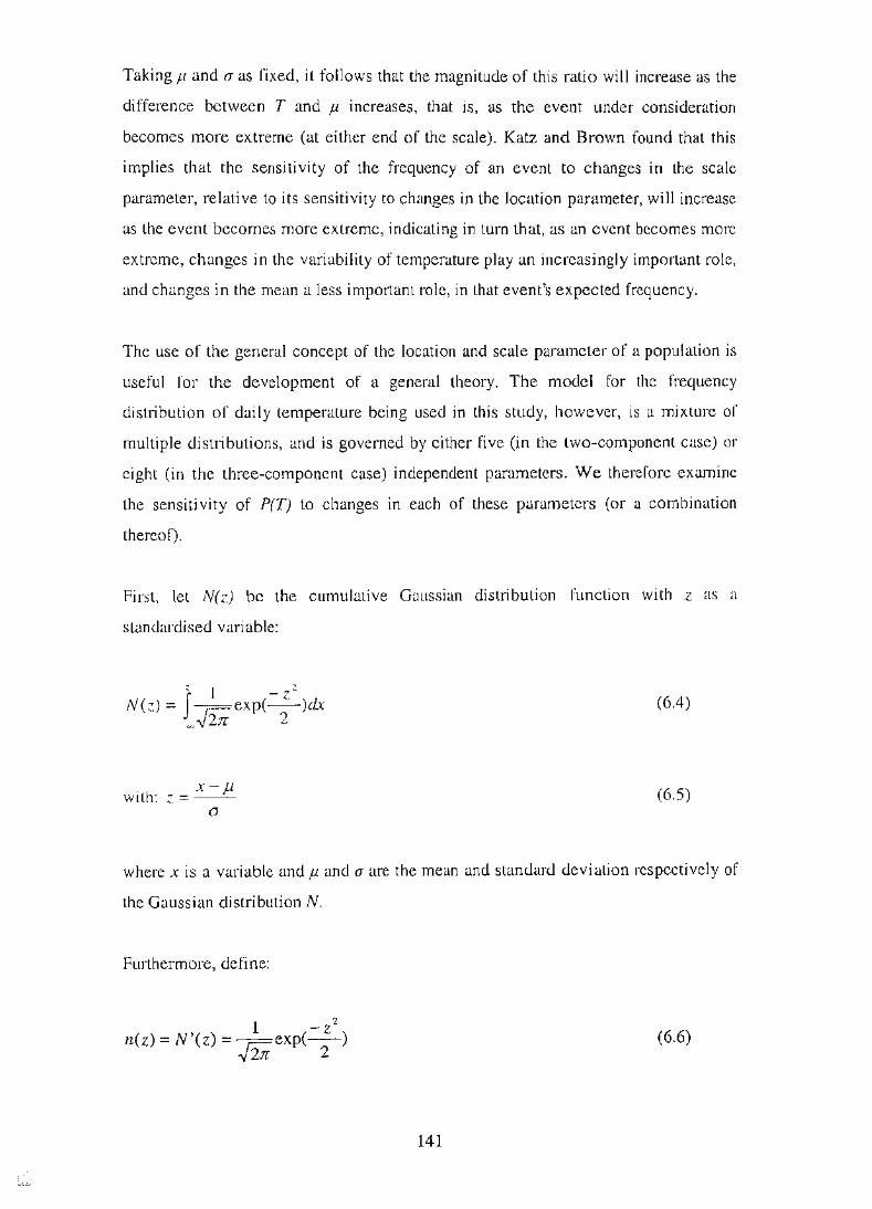
Taking J-l and a as fixed, it follows that the magnitude of this ratio will increase as the
difference between T and f.i increases, that is, as the event under consideration
becomes more extreme (at either end of the scale). Katz and Brown found that this
implies that the sensitivity of the frequency of an event to changes in the scale
parameter, relative to its sensitivity to changes in the location parameter, will increase
as the event becomes more extreme, indicating in turn that, as an event becomes more
extreme, changes in the variability of temperature play an increasingly important role,
and changes in the mean a less important role, in that event's expected frequency.
The use of the general concept of the location and scale parameter of a population is
useful for the development of a general theory. The model for the frequency
distribution of daily temperature being used in this study, however, is a mixture of
multiple distributions, and is governed by either five (in the two-component case) or
eight (in the three-component case) independent parameters. We therefore examine
the sensitivity of P(T) to changes in each of these parameters (or a combination
thereof).
First, let N( z) be the cumulative Gaussian distribution function with z as a
standardised variable:
z 1 - 22 N(z) = J ~exp(-· )dx
-<XJ '\/ 2:rr 2 (6.4)
with: x-p.
z=-- (6.5) 0
where xis a variable and panda are the mean and standard deviation respectively of
the Gaussian distribution N.
Furthermore, define:
1 - z2
n(z) = N'(z) = ~exp(-) ""277: 2
(6.6)
141

We may then define the cumulative distribution for the two-component compound
Gaussian distribution as follows:
(6.7)
where the two components have weights WJ and w2, means /11 and 1t2 and standard
deviations CJ1 and a2 respectively.
Using the result from equation 6.3, the following relationships, analogous to those
found by Katz and Brown (1992) for a single distribution, follow from the definition
in 6.7:
(6.8)
(6.9)
These results imply that the sensitivity of the frequency or a temperature above or
below a given threshold becomes more sensitive to the variability of that component,
relative to the mean, as the threshold departs further from the mean of the component.
The simplicity of these results depends on the fact that n(z) (or F'(z) in the more
general results of Katz and Brown) cancels out. The absence of such a cancellation
involving 8F/8w 1nakes it more complex to examine the sensitivity of the frequency of
temperatures above or below a threshold to changes in component weights. (The
interpretation of the results is also clouded by the fact that the weights are
dimensionless, whereas the means and standard deviations are measured using the
same units).
142

We may still develop a relationship involving the weights in some cases. In parts of
the composite distribution which are only substantially contributed to by one
component (as is usually the case in the two tails of the distribution), and assuming
that fl. I ::::; f.L 2 , then, for low T, we have:
(6.10)
and for high T:
( 6.11)
Using the fact that N(z) = 1 - N( -z) , we then have for low T:
,dF :::::: N ( T - tL 1 )
awl 0"1 (6.12)
and for high T:
()F JI, -T -,-:::::N(- ) awl 0" 2
(6.13)
143

Using this and the fact that n(z) = n(-z), we may obtain the following relationships, for
lowT:
(6.14)
(6.15)
For high T we have:
(6.16)
(6.17)
Over the range -4 < z < 0, the ratio n(z)IN(z) is approximately a linear function of z
(Fig. 6.6), and hence ofT (as z is a linear function of T). It hence follows that, as the
departure of a threshold from a component mean increases, the sensitivity of the
frequency of temperatures above or below that threshold to the weights decreases
relative to the sensitivities to both the mean and standard deviation.
144

Fig. 6.6. n(z)/N(z), as defined in section 6.5
0.05
0.045
0.04
0.035
0.03
'N z :::::. 0.025 N c:
0.02
0.015
0.01
0.005
0
-4 -3.5 -3 -2.5 -2 -1.5 -1 -0.5 0
z

The following order of importance then follows as a threshold becomes more
extreme:
1. Standard deviation
2. Mean
3. C01nponent weight
in determining the frequency of temperatures above or below that threshold.
The generalisation to the three-component case is more complex, as the set of
component weights w J, w2 and W3 has two degrees of freedom, rather than one, and it
is not possible to isolate a part of the overall distribution where the third co1nponent is
dominant, as the distribution has only two tails. These two factors combine to prevent
a generalisation of equations 6.10 to 6.17. The relationships of sensitivities to means
and standard deviations shown in 6.8 and 6.9, however, do hold for a third
component.
As a result of the difficulties in the theoretical treatment of the three-component case,
the attempts to relate observed changes in extre1ne event frequency to changes in
parameters of the distributions, described in Chapter 7, will concentrate on those
stations and months where the frequency distribution has been shown to be adequately
represented by two Gaussian components.
6.6. Sun1n1ary
In this chapter, the compound Gaussian distribution has been developed as an
appropriate frequency distribution for the representation of daily maximum and
minimum temperatures. This model will be used further in Chapter 7, in order to
assess changes over the 1957-96 period in the nature of the frequency distribution of
daily maximum and minimum temperature, and to make conclusions from these
changes concerning the potential attribution of such changes to physical causes.
145

Chapter 7
Observed Changes in the Frequency of Threshold
Temperature Events at Australian Stations
7.1. Observed trends in frequency of threshold events at individual stations
7 .1.1. Methods
Trends in the frequency of threshold events were considered in a number of ways. The
following types of events were considered as possible threshold events for
investigation:
(a) The frequency of temperatures above or below a percentile threshold
Events examined were the monthly frequency of daily maximum and minimum
temperatures above the 90th and 95th percentiles, and below the 5th and 1Oth
percentiles. In each case, the temperatures used were the deseasonaliscd anomalies as
defined in Chapter 6.
The pcrcenti le thresholds were calculated separately for each of the 12 calendar
months. As anomalies from a normal which varies seasonally, the absolute
temperature cotTesponding to a given percentile threshold will vary through a month,
particularly in spring and autumn.
147

(b) The frequency of temperatures above or below a fixed threshold
Events examined were the monthly frequency of daily max1mum or minimum
temperatures breaching the following thresholds:
• Maxima above 40, 35 and 30°C
• Minima above 20°C
• Maxima below 10 and l5°C
• Minima below 5, 2 and ooc
In each case, the number of events per month was aggregated to generate four
seasonal totals per year, for summer (December-February), autumn (March-May),
winter (June-August) and spring (September-November). The number of events per
season was then divided by the number of observations to generate the number of
events per season as a proportion of all observations, in order to take missing
observations into account.
Trends were calculated for each threshold and season over the 1957-96 period
(although some stations were not open for the full period of record). At stations for
which data arc available prior to 1950, trends were also calculated for the full period
of record at those stations.
In the case of fixed-threshold events, no trend was calculated if the event did not
occur at least once in 20o/o of seasons, or if it occuned on every day in at least 20% of
seasons. This prevents trends from being calculated if the event is rare or unknown at
that station and season. (For example, at Thursday Island, where no temperature
below 19.5oc has ever been observed between October and June, a trend in the
frequency of summer or autumn minima above 20°C, or below 5° or 0°C, would
obviously be meaningless).
Following the arguments of Nicholls (2001), it has not been considered appropriate to
carry out significance testing on the trends, as the data from the 1957-1996 period are
being viewed as a set of observations in itself and not as a sample from a larger
148

statistical population. In any case, the magnitude of the observed trend is of greater
importance than its statistical significance (Nicholls, 2001). As a benchmark,
particular attention will be drawn in this section to trends exceeding 5 days/decade at
the annual timescale. When the lOth and 90th percentile thresholds are being
considered, an increasing trend of 5 days/decade represents an increase in frequency
of 75% over the 1957-1996 period, whilst a similar decreasing trend represents a
decrease in frequency of 43% over the same period.
As is discussed in more depth in Chapter 8, the percentile thresholds are most
appropriate to any consideration of events on a national basis, as they occur with
equal frequency over the long term at each station and in each season. A fixed
threshold can also represent a different type of event at different stations: the
frequency of winter maximwn temperatures below IOOC is a indicator of extren1c low
1naxima in many parts of Australia, but at the alpine site of Cabramurra it is an
indicator of extreme high maxima (for the season).
It is, however, useful to consider fixed absolute thresholds at individual stations to
which they are appropriate, not least because of the physical significance of some of
the thresholds - for example, the importance of frost frequency in agriculture. Some
discussion of the significance of such thresholds is worthwhile at this point. In some
cases (such as frost) a specific threshold is critical. In other cases, while studies of the
itnpacts of extreme events have focused on specific thresholds, these thresholds arc
themselves somewhat arbitrary choices. Australian examples of the i1npact or extreme
high temperatures on crop yields and quality (e.g. Savin and Nicolas, 1999; Savin ct
al., 1996; Blumenthal et al., 1991) have found relationships between crop yield and
quality and the occurTence of temperatures above a specific threshold, but in these
cases the impact of high temperatures was gradual (i.e. there was a progressive change
in yield with increasing temperature, rather than a sudden change at a specific
threshold) and the choice of a specific threshold for analysis is somewhat arbitrary.
Elsewhere, the impact of extreme high temperatures on wheat and corn yields in the
United States has been the subject of much study (e.g. Mearns et al., 1991 ). However,
Shaw ( 1983) 's discussion of climatic influences on corn yields suggests that the
impact of temperature on yields is also one which changes gradually with an increase
in the threshold used.
149
-
Current international research on indices of climate extremes (e.g. IPCC, 2001) uses a
variety of thresholds (both fixed and non-fixed), many of which are also arbitrary in
nature.
The major urban stations were included in this stage of the analysis. Whilst the
observed trends from those stations cannot be taken as representative of broader
climate change, the nature of the changes in the frequency of threshold exceedances
and how they relate to changes in the frequency distribution are still of interest,
whatever the underlying cause.
7.1.2. Results for the 1957-1996 period
The observed trends in the frequency of exceedances of high percentile thresholds are
shown in Figs. 7.la-h, and in Tables 7.1a-h. Those in the frequency of cxceedances of
fixed thresholds are shown in Figs. 7.2a-i, and in Tables 7.2a-i. All trends are shown
in terms of days per decade, converting the proportion of threshold days to a number
of days assuming a full set of observations for each season (and assuming a 28-day
February).
The signs of the observed trends arc summarised in Tables 7 .] and 7 .4.
150

'/.r
~ \ J.~/
Spring ')j
50
4
-1
·2
·3
-4
-50
50
2
1
0
·1
·2
·3
-4
·50
50
10
5
-5
·10
·50
·~
50
4
3
2
1
0
·1
-2
·3
·4
·50
50
4
3
2
1
0
·1
·2
·3
·4
·50
Fig. 7.la. Trends, days/decade, in frequency of maxima above 95th percentile

\
~ - / t.O
Spring ' ~j
' ~~
50
4
3
2
1
0
-1
·2
·3
-4
-50
50
4
3
-1
-2
-3
-4
-50
50
10
5
0
-5
-10
-50
50
4
3
2
0
-1
·2
-3
-4
'ti ·50
50
4
3
(Q !·
2
1
0
\· iJ~o -1
·2
"--'{Jiii? '~I ·~. 0 -3
-4 \. .. ,,
-50 Winter ' t;j
Fig. 7.1 b. Trends, days/decade, in frequency of maxima above 90th percentile

50
4
3
·1
·2
·3
·4
·50
50
4
3
2
1
0
·1
·2
-3
·4
-50
50
10
5
-5
·10
!,
-50 i l
50
4
3
2
1
0
·1
·2
-3
-4
·50
50
4
3
2
0
·1
·2
-3
-4
-50
Fig. 7 .lc. Trends, days/decade, in frequency of minima above 95th percentile

50
4
3
2
1
0
-1
-2
-3
-4
-50
50
4
3
-1
-2
·3
·4
-50
50
10
5
0
-5
-10
-50
'rj
I
t;;)
50
4
3
2
1
0
-1
-2
-3
-4
-50
50
4
3
2
1
0
-1
-2
-3
-4
-50
Fig. 7.1 d. Trends, days/decade, in frequency of minima above 90th percentile

50
4
·1
·2
·3
·4
-50
50
4
3
·1
-2
·3 -4
-50
50
10
5
·5
·10
·50
'tj
50
4
3
2
1
0
-1
·2
·3
-4
-50
50
4
3
2
1
0
-1
-2
-3
-4
-50
Fig. 7.1 e. Trends, days/decade, in frequency of maxima below 1Oth percentile
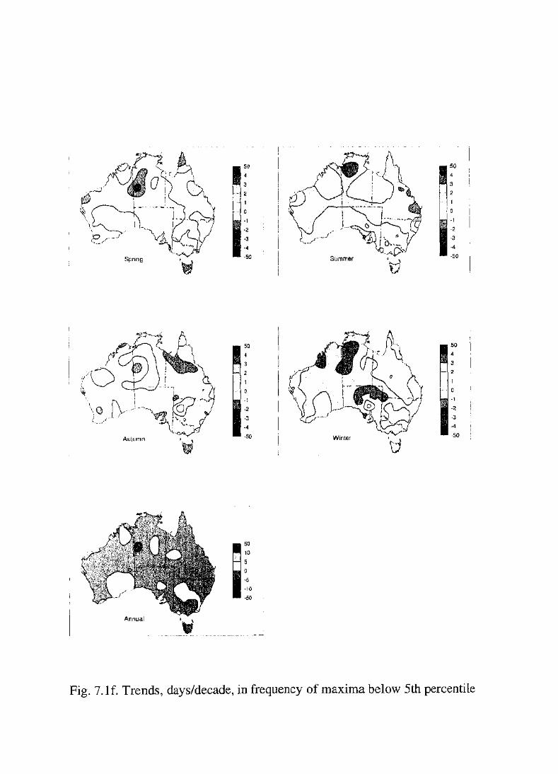
,v I (
~ ' ~; ~· F"'j ... )-
l ... , •.. ~/
Autumn
50
·1
-2
-3
-4
-50
50
10
5
0
-5
-10
-50
'tj
50
4
3
2
1
0
-1
-2
-3
-4
I -50
tJ
Fig. 7.lf. Trends, days/decade, in frequency of maxima below 5th percentile

'tj
. t;j
50
-1
-2
-3
-4
-50
50
4
3
2
1
0
-1
-2
-3
-4
-50
50
10
-5
-10
-50
·~
' tr;i
50
4
3
2
1
0
-1
-2
-3
-4
-50
50
4
3
2
1 0
-1
-2
-3
-4
-50
Fig. 7.1g. Trends, days/decade, in frequency of minima below lOth percentile

·~
' \;}
50
·1
·2
-3
·4
-50
50
4
2
1
0
·1
-2
-3
-4 -50
50
10
5
-5
-10
-50
'(;}
·~
50
4
3
2
0
-1
·2
-3
-4
-50
50
4
3
2
0
-1
·2
-3
-4
-50
Fig. 7 .I h. Trends, days/decade, in frequency of minima below 5th percentile

Spring ' t}
50
·1
·2
·3
-4
·50
50
4
3
2
1
0
·1
·2
-3
·4
·50
50
10
5
0
-5 -10
-50
Winter
. tJ
50
4
3
2
1
0 _, ·2
-3
-4
-50
50
4
3
2
1
-1
-2
3
-4
-50
Fig. 7 .2a. Trends, days/decade, in frequency of maxima above 30 degrees C

Spring
'""•r' Autumn ·'
\)
50
4
-1
-2
-3
-4
-50
50
4
-1
-2
-3
-4
-50
50
10
5 0
-5
-10
-50
... "/
r ~
\ .• l
/j 'l.fr, '"')
Winter
50
4
3
2
1
0
-1
-2
-3
-4
' -50
\j
ti 50 r I 4
3
2
1
0
-1
-2
·3
-4 .... ,
-50 '
... (·.'i !,,!
Fig. 7 .2b. Trends, days/decade, in frequency of maxima above 35 degrees C

'/"' /.4:,1
(If I I
~I
\ I
Spring
50
4
3
-1
·2
-3
·4
-50
50
4
2
-1
·2
-3
-4
·50
50
10
5
-5
·10
·50
50
4
3
2
0
-1
-2
-3
-4
Summer -50
Fig. 7 .2c. Trends, days/decade, in frequency of maxima above 40 degrees C

Spring
()
Autumn r.lf..l.: .• r,-
\)
50
-1
-2
-3
-4
-50
50
4
3
2
1
0
-1
-2
-3
-4
-50
50
10
5
0
-5
-10
-50
t=~-·'?a /'"~~ a
!'
Summer
~I' (11 I I
~~ \
\
J "•t. tl \::rr'i '")
Winter
50
4
3
2
1
0
-1
-2
-3
-4 . -50
(j
50
4
3
2
1
'f. 0
.. -J -1 I
/ ·2
/ -3 I
; J -4 ...... ·50 ' (' • ? t,~
Fig. 7 .2d. Trends, days/decade, in frequency of minima above 20 degrees C

/
f I
\i,l
~.
..,-,1··· / t·, , .. "7n I~ ~ .r' ,{ ('ll i .. , f K• .
('? ', .. , r I I l
l \
.\,'"t
- ir;;J Vlt" ~· Spring
~;:"t···i
(x1 ' 1
!.""~ '
Autumn
't,j
\" /\ ~ ( / -~ : ~
I \
50
·1
·2
·3
·4
·50
50
4
3
·1
-2
-3
-4
-50
50
10
5 0
-5
-10
-50
';.,...
~I I
~ \
\ )
~~--~ r~. /''~ -~ ) L . 50
A, I .... I ( I . I '·. \ 4
j I 3 '\ 2 ~\
'r 0
' ~ -1 I
~~t, A • I -2 I
<.{ J[) ; \, r:f -3 -~· ... ~~
. \: "·-·. -4
Summer ....... .A.,..,.
-50
·~
k:>"i'~ i ,1' ~ • r. f·',~ ,·a 50 · r I ;"·! ! I .. \
4
3
2
0
·1
·2
·3
-4
Winter -50
Fig. 7 .2e. Trends, days/decade, in frequency of maxima below 15 degrees C

{\ j \ •. ,
' ;" I I r ~
I
~I
. I
Spring
::·, ... ~ ~ / i"'ll f K',.t I
r·'\~ ~
"\ ,,.
... 'f I
Autumn ' ., A~.:·~'•· ·-"""~
,..:"' ,. ~1
x··J;. I /,~/ I
~
Annual
50
·1
·2
·3
·4
·50
50
·1
-2
-3
·4
-50
50
10
5
0
·5
-10
-50
~I
I
~.
' \ \ )
Summer
~?:\'···i r'
{")~l '· rv : , I'
I
Winter
50
4
3
2
1
0
-1
-2
-3
-4
-50
50
4
3 2
1
0
·1
·2
-3
·4
-50
Fig. 7 .2f. Trends, days/decade, in frequency of maxima below 10 degrees C

' ~I
50
-1
-2
-3
-4
-50
50
4
3
-1
-2
-3
-4
-50
50
10
5
0 -5
-10
-50
~f
I ~I
.. ~/"
50
4
3
2
1
0
-1
-2
-3
-4
-50
50 4
3
0
-1
-2
·3
-4
·50
Fig. 7 .2g. Trends, days/decade, in frequency of minima below 5 degrees C

?~-;> (" / >'>l I
/":~ '. ,,,
(! ' ',, j \
l,v
,. 'l;!•
••
I
~~
Autumn
50
4
3
2
0
-1
-2
-3
-4
-50
50
-1
-2
·3
·4
-50
50
10
5
-5
-10
-50
50
4
3
2
1
0
-1
·2
·3
·4
-50
Fig. 7 .2h. Trends, days/decade, in frequency of minima below 2 degrees C

~I
Autumn
50
-1
-2
-3
-4
-50
50
4
3
1
0
-1
-2
·3
-4
-50
50
10
5
0
-5
-10
-50
50
4
3
2
0
·1
-2
-3
-4
-50
Fig. 7 .2i. Trends, days/decade, in frequency of minima below 0 degrees C

Table 7.la. Trends in frequency of ntaxima above 95th percentile, 1957-96
Station Station name Trend (days/decade) number Spring Summer Autumn Winter Annual 1021 Kalurnburu -0.12 0.94 3.04 1.17 4.96 2012 Halls Creek -0.72 -1.88 -1.25 -0.47 -4.11 3003 Broome 0.82 0.19 0.36 1.65 2.95 4032 Port Hedland 0.40 0.49 0.46 0.28 1.55 5007 Lcarmonth 0.70 -0.64 0.97 0.49 1.96 5026 Wittenoom 0.22 1.29 0.55 0.23 2.23 6011 Carnarvon -0.37 -0.66 0.24 -0.18 -0.96 7045 Meekatharra 0.32 0.58 -0.06 0.51 1.27 8039 Dalwallinu 0.28 -0.10 -0.02 0.73 0.93 8051 Gerald ton 0.11 -0.11 0.15 0.20 0.30 9021 Perth Airport 0.02 -0.12 -0.23 0.07 -0.38 9518 Cape Leeuwin 1.02 -0.06 0.00 0.18 1.24 9741 Albany -0.25 -1.14 0.05 0.28 -1.15 9789 Esperance -0.09 -1.02 0.02 -0.58 -1.66 10035 Cunderdin 0.62 0.02 0.30 0.38 1.30 10648 Wandering 0.52 -0.32 -0.10 0.36 0.56 11052 Forrest 0.16 0.43 0.34 0.66 1.47 12038 Kalgoorlie 0.66 0.20 0.15 0.66 1.62 13017 Giles 0.69 0.92 1.09 0.35 3.05 14015 Darwin Airport -0.12 -0.40 0.24 0.21 -0.21 14825 Victoria River Downs* 0.25 -0.62 1.72 0.90 1.94 15135 Tennant Creek 1.84 0.31 -1.33 0.97 1.92 15548 Rabbit Flat* 4.54 2.11 2.10 4.82 13.79 15590 AI ice Springs 0.70 1.42 0.00 0.99 3.10 16001 Woomera -0.16 -0.67 -1.22 0.86 -1.22 16044 Tarcoola 0.97 1.56 1.95 1.14 5.58 17031 Marrec -0.09 0.32 -0.31 -0.03 -0.13 17043 Oodnadatta 0.98 1.20 0.42 0.11 1.93 18012 Ceduna 0.09 0.04 0.06 0.65 0.79 18070 Port Lincoln -0.22 -0.33 -0.04 0.62 0.05 21046 Snowtown 0.43 -0.43 0.75 0.51 0.85 22801 Cape Borda 0.86 0.16 0.73 0.64 2.30 23090 Adelaide RO 0.24 0.17 0.39 0.69 1.39 23373 Nuriootpa -0.20 0.03 0.84 0.12 0.79 26021 Mount Gambier -0.13 0.00 0.47 0.37 0.62 2602() Robe 0.47 -0.37 0.95 0.06 1.07 27022 Thursday Island 1.39 1.59 -1.99 -0.78 0.47 27045 Weipa -1.59 -1.63 2.09 -2.38 -3.32 28004 Palmerville 1.16 1.71 0.79 1.36 4.97 29004 Burketown -0.35 -0.61 -1.45 -0.74 -2.91 30045 Richmond -0.32 -0.45 0.26 -0.70 -0.93 31011 Cairns 1.71 0.43 1.10 1.12 4.35 32040 Townsville 0.45 1.79 2.56 0.44 5.13 33119 Mackay MO 1.91 2.65 0.74 0.91 6.25 34084 Charters Towers 0.00 1.59 1.14 0.28 3.08 36007 Barca! dine 0.50 0.58 0.54 1.23 2.89 36031 Longreach -0.20 -0.64 -0.45 0.24 -0.85 37010 Camooweal 0.57 1.27 -0.42 1.40 2.75 38002 Birds ville 0.63 0.74 -0.11 1.38 2.62 38003 Boulia -0.03 1.42 -0.02 0.94 2.16 39039 Gayndah 1.05 1.29 0.03 1.25 3.57 39083 Rockhampton 0.38 0.77 0.12 0.14 1.51

Table 7.1a (cont.). Trends in frequency of maxima above 95th percentile, 1957-96
Station Station name Trend (days/decade) number Spring Summer Autumn Winter Annual 39128 Bundaberg 0.57 1.42 0.33 0.27 2.51 40004 Amberley 1.07 0.38 -0.03 1.06 2.67 40223 Brisbane Airport -0.15 -0.25 -1.69 -0.48 -2.42 40264 Tewantin 1.80 0.44 -0.23 1.13 2.73 42023 Miles 0.14 0.43 0.11 1.70 2.45 43109 St. George 0.59 -0.63 -0.28 1.00 0.74 44021 Charleville 0.46 0.73 0.05 0.69 1.95 45017 Thargomindah -0.29 0.16 -0.3() 0.80 0.06 46037 Tibooburra 0.18 0.96 0.18 0.94 2.31 46043 Wilcannia -0.79 -0.22 -0.49 0.31 -1.24 48027 Co bar 0.00 -0.04 -0.26 0.86 0.42 48239 Bourke 0.19 0.35 -0.91 0.88 0.42 52088 Walgett 0.20 -0.05 -0.28 0.44 0.07 53048 Moree 0.00 -0.35 -0.91 -0.97 -2.24 55024 Gunnedah Soil Cons -0.37 -0.08 -0.96 0.84 -0.90 56017 Inverell PO 0.87 0.44 -0.32 -0.19 0.81 58012 Yamba 0.75 0.69 0.43 0.92 2.76 59040 Coffs Harbour 0.08 0.10 -0.41 0.24 0.02 60026 Port Macquarie 0.73 2.37 1.19 1.2() 5.58 61078 Williamtown 0.49 0.51 -0.80 0.85 1.14 61089 Scone Soil Cons 0.31 -0.60 -0.57 0.80 -0.28 63005 Bathurst ARS -0.31 0.41 -0.()0 -0.09 -0.71 65012 Dubbo -0.19 -0.04 0.05 0.47 0.26 66062 Sydney RO 0.06 -0.07 -0.55 0.44 -0.12 67105 Richmond 0.25 0.51 -0.27 0.45 0.95 68034 Jervis Bay 0.24 -0.15 -0.55 0.48 -0.08 68076 Nowra 0.01 -1.24 -0.45 -0.49 -2.08 69018 Moruya Heads 0.39 -0.40 -0.27 0 .() I -0.31 70014 Canherra Airport -0.56 -0.02 0.05 0.73 0.10 72150 Wagga Wagga -0.48 0.48 0.37 0.12 0.38 72161 Cahramurra -0.22 -0.17 -0.31 0.()4 -0.01 73054 Wyalong 0.72 -0.02 -0.31 1.00 1.66 74128 Dcniliquin 0.03 0.()7 0.24 -0.25 0.()7 76031 Mil dura -0.53 -0.20 -0.4<) 0.15 -1.18 78031 Nhill -0.02 0.46 0.19 0.05 0.72 80023 Kerang 0.39 0.18 0.13 0.71 1.39 82039 Rutherglen -0.15 0.04 0.53 0.08 0.32 84016 Gaho Island -0.40 -0.27 -1.03 0.()2 -1.04 84030 Orbost -0.21 -0.42 -0.64 -0.92 -2.42 85072 Sale -0.56 -0.12 0.22 0.93 0.40 85096 Wilsons Promontory 1.10 -0.20 0.25 0.73 1.84 86071 Melbourne RO -0.07 -0.25 0.19 0.02 -0.22 87031 La vert on 0.24 -0.60 0.46 0.73 0.72 90015 Cape Otway 0.48 -0.15 0.07 0.42 0.56 91057 Low Head 0.11 -0.49 1.12 1.24 2.05 91104 Launceston AP -0.46 -0.17 0.76 0.42 0.35 92045 Eddystone Point 0.25 0.27 1.03 2.10 3.61 94010 Cape Bruny -0.22 -0.52 0.07 0.22 -0.45 94029 Hobart RO 0.42 0.11 0.41 0.71 1.58 94069 Grove 0.58 -0.38 0.52 0.67 1.28 96003 Butlers Gorge 1.15 0.67 1.08 0.28 3.29 *denotes statiOn w1th less than 35 years of record m the 1957-96 penod

Table 7.1 b. Trends in frequency of maxima above 90th percentile, 1957-96
Station Station name Trend (d~ys/decade) nurnher Spring Summer Autumn Winter Annual 1021 Kalumburu -0.22 0.58 5.55 1.93 8.00 2012 Halls Creek -1.19 -3.62 -1.69 -0.70 -6.90 3003 Broome 1.05 -0.05 0.52 2.68 4.02 4032 Port Hedlaml 0.15 0.39 0.44 0.68 1.53 5007 Leannonth -0.06 -0.39 1.43 0.49 1.82 5026 Wittenoom 0.92 2.32 1.51 0.92 5.47 6011 Carnarvon -0.89 -0.84 0.66 0.13 -0.99 7045 Meckatharra 0.48 0.51 0.02 1.09 2.01 8039 Dalwallinu 0.23 0.00 -0.03 1.02 1.21 8051 Gerald ton 0.14 0.00 0.57 0.50 1.07 9021 Perth Airport 0.43 -0.23 0.29 0.40 0.72 9518 Cape Lceuwin 1.64 -1.27 -0.09 0.13 0.56 9741 Alhany -0.62 -2.21 0.99 0.47 -1.44 9789 Esperance 0.25 -0.99 -0.61 -1.42 -2.80 10035 Cunderdin 0.56 -0.16 0.00 1.10 1.48 10648 Wandering 0.62 -1.32 -0.16 0.54 -0.10 11052 Forrest 0.11 0.17 0.44 0.84 1.25 12038 Kalgoorlie 0.75 0.56 0.12 0.82 2.09 13017 Giles 1.04 1.50 1.63 0.36 4.67 14015 Darwin Airport -0.05 -0.50 0.54 1.16 0.84 14825 Victoria River Downs* 0.12 -1.12 2.36 0.71 1.28 15135 Tennant Creek 2.12 0.29 -1.45 0.82 1.96 15548 Rahhit Flat* 7.10 3.22 5.29 4.74 21.00 15590 Alice Springs 1.42 1.79 0.04 1.32 4.61 16001 Woomera -0.52 -1.50 -0.93 -0.51 -3.50 1Cl044 Tarcoola 1.66 1.98 2.32 2.00 7.98 17031 Marrec -0.06 0.91 -0.10 0.05 0.82 17043 OoJnadatta 1.64 2.49 0.71 0.63 3.78 18012 Ceduna -0.20 0.02 -0.37 0.20 -0.48 18070 Port Lincoln 0.48 -0.11 0.01 1.02 1.44 21046 Snow town 0.19 -0.57 1.02 0.26 0.28 22801 Cape BorJa 1.19 0.31 1.15 0.75 3.40 23090 Adelaide RO 0.05 -0.03 0.61 -0.05 0.42 23373 Nuriootpa -0.07 0.19 0.87 0.47 1.40 26021 Mount Gambier -0.43 0.12 0.53 0.23 0.24
2602C> Rohe 0.45 -0.35 1.40 0.61 1.82 27022 Thursday Island 2.49 3.07 -1.03 -1.06 3.97 27045 Weipa -2.64 -3.17 2.96 -4.14 -7.33 28004 Palmcrvi lle 1.73 2.28 1.17 1.00 6.15 29004 Burketown -0.66 0.08 -2.26 -1.53 -3.68 30045 Richmond -0.65 -0.79 0.78 -0.78 -0.98 31011 Cairns 2.30 0.35 1.07 2.14 5.92 32040 Townsville 0.84 3.54 4.81 0.99 10.25 33119 Mackay MO 3.43 4.13 0.37 0.62 8.65 34084 Charters Towers -0.47 3.09 2.76 0.89 6.23 36007 Barcaldine 1.36 0.84 1.24 1.39 4.84 36031 Longreach -0.45 0.12 0.33 0.44 0.65
37010 Camooweal. 0.63 2.24 -0.19 2.04 4.55
38002 Birds ville 0.85 1.15 -0.39 1.61 3.23 38003 Boulia -0.02 2.15 1.00 1.27 4.23 39039 Gayndah 1.72 2.07 -0.04 2.05 5.74 39083 Rockhampton 1.27 0.91 0.56 0.61 3.41
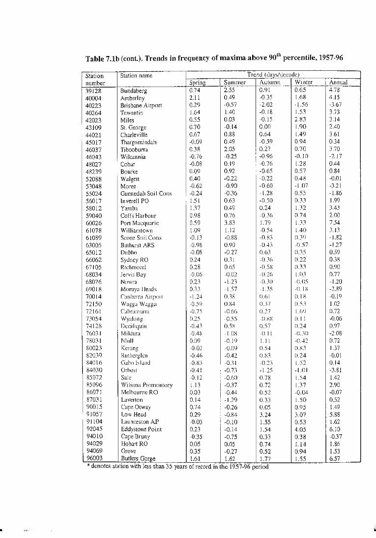
Table 7.1b (cont.). Trends in frequency of maxima above 90th percentile, 1957-96
Station Station name Trend (days/decade) number Spring Summer Autumn Winter Annual 39128 Bundaberg 0.74 2.55 0.91 0.65 4.78
40004 Amber ley 2.11 0.49 -0.35 1.68 4.15
40223 Brisbane Airport 0.29 -0.57 -2.02 -1.56 -3.67
40264 Tewantin 1.64 1.40 -0.18 1.53 3.73
42023 Miles 0.55 0.03 -0.15 2.83 3.14
43109 St. George 0.70 -0.14 0.00 1.90 2.40
44021 Charleville 0.67 0.88 0.64 1.49 3.61 45017 Thargomindah -0.09 0.49 -0.59 0.94 0.34 46037 Tibooburra 0.38 2.05 0.27 0.70 3.70 46043 Wilcannia -0.76 -0.25 -0.96 -0.10 -2.17 48027 Co bar -0.08 0.19 -0.7() 1.28 0.44 48239 Bourke 0.09 0.92 -0.65 0.57 0.84 52088 Walgett 0.40 -0.22 -0.22 0.48 -0.01 53048 Moree -0.62 -0.90 -0.60 -1.07 -3.21 55024 Gunnedah Soil Cons -0.24 -0.36 -1.28 0.55 -1.86 56017 Inverell PO 1.51 0.63 -0.50 0.33 1.99 58012 Yamba 1.37 0.49 0.24 1.32 3.43 59040 Coft's Harbour 0.98 0.76 -0.3() 0.74 2.00 60026 Port Macquarie 0.59 3.83 1.79 1.33 7.54 61078 Williamtown 1.09 1.12 -0.54 1.40 3.13 61089 Scone Soil Cons -0.13 -0.88 -0.83 0.39 -1.82 63005 Bathurst ARS -0.98 0.90 -0.43 -0.57 -1.27 65012 Dubbo -0.08 -0.27 ().()3 0.35 0.59 66062 Sydney RO 0.24 0.31 -0.3() 0.22 OJ8 67105 Richmond 0.28 0.()5 -0.5X 0.33 0.90 68034 .Jervis Bay -0.06 -0.02 -0.2() 1.03 0.77 68076 Nowra 0.23 -1.23 -0.30 -0.05 -1.20 69018 Moruya Heads 0.33 -1.57 -1.35 -0. I R -2.89 70014 Can berra Airport -1.24 0.38 0.()] 0.1 X -0.19 72150 Wagga Wagga -0.59 0.84 0.37 0.5J 1.02 72161 Cahramurra -0.75 -0.66 0.27 I .U) 0.72 73054 Wyalong 0.25 -0.55 -O.XX 0.11 -0.06 74128 Dcniliquin -0.43 0.58 0.57 0.24 0.97 76031 Mildura -0.48 -1.08 -0. I I -0.30 -2.08 78031 Nhill 0.09 -0.19 I. 1 I -0.42 0.72 80023 Kerang -0.02 -0.09 0.54 O.X3 1.37 82039 Rutherglen -0.46 -0.42 0.83 0.24 -0.01 84016 Gaho Island -0.83 -0.31 -0.23 1.52 0.14 84030 Orhost -0.41 -0.73 -1.25 -1.0 I -3.81 85072 Sale -0.12 -0.60 0.78 1.54 1.42 85096 Wi !sons Promontory 1.13 -0.37 0.72 1.37 2.90 86071 Melbourne RO 0.03 -0.44 0.52 -0.04 -0.07 87031 La vert on 0.14 -1.29 0.33 1.50 0.52 90015 Cape Otway 0.74 -0.26 0.05 0.95 1.49 91057 Low Head 0.29 -0.84 3.24 3.07 5.88 91104 Launceston AP -0.03 -0.10 1.55 0.53 1.62 92045 Eddystone Point 0.23 -0.14 1.54 4.05 6.10 94010 Cape Bruny -0.35 -0.75 0.33 0.38 -0.37 94029 Hobart RO 0.05 0.05 0.74 1.14 1.86 94069 Grove 0.35 -0.27 0.52 0.94 1.53 96003 Butlers Gorge 1.61 1.62 1.77 1.55 6.57 *denotes statiOn w1th less than 35 years of record in the 1957-96 period

Table 7.1c. Trends in frequency of minima above 95th percentile, 1957-96
Station Station name Trend (days/decade) number Spring Summer Autumn Winter Annual 1021 Kalumburu 1.49 0.60 1.17 -0.17 3.36 2012 Halls Creek -0.31 -1.44 -0.58 -1.08 -3.17 3003 Broome 2.39 1.56 -0.31 0.05 3.77 4032 Port Hedland 0.53 0.12 0.79 0.94 2.33 5007 Lear month -0.48 -3.76 -1.23 1.29 -3.23 5026 Wittcnoom 0.27 0.20 0.65 0.54 1.54 6011 Carnarvon 0.13 1.33 0.38 0.87 2.76 7045 Meckatharra 0.46 0.23 0.73 0.31 1.62 8039 Dalwallinu 0.48 -0.66 -0.14 0.11 -0.17 8051 Geraldton 0.66 -0.38 0.78 0.59 1.66 9021 Perth Airport 1.82 0.85 1.13 0.15 3.89 9518 Cape Leeuwin 1.71 -0.21 0.86 1.42 3.81 9741 Albany 0.01 -0.45 1.33 1.19 1.96 9789 Esperance 0.90 0.69 1.00 0.66 3.28 10035 Cunderdin 0.61 -0.64 -0.03 0.76 0.81 10648 Wandering 0.75 -0.62 -0.02 0.77 1.15 11052 Forrest 1.78 0.07 1.20 0.76 3.87 12038 Kalgoorlie 1.10 0.71 1.12 1.17 4.02 13017 Giles -0.09 1.28 0.41 -0.45 1.20 14015 Darwin Airport 1.84 0.83 1.78 0.96 5.38 14825 Victoria River Downs* 1.86 -0.30 1.54 -0.20 2.94 15135 Tennant Creek 0.65 0.78 1.56 1.17 4.21 15548 Rahhit Flat* 1.43 1.56 1.59 0.68 5.27 15590 Alice Springs -0.04 -0.09 -0.32 1.55 1.07 16001 Woc)mera -0.60 -1.06 -0.23 1.15 -0.40 I6044 Tarcoola 0.09 1.12 0.71 -0.21 1.71 17031 Man·ce -0.62 -0.31 0.71 -0.29 -0.50 17043 Oounadatta -0.20 -0.80 0.54 1.48 0.95 18012 Ceduna 0.81 -0.27 0.35 0.27 1.11 18070 Port Lincoln 0.69 0. I 1 0.41 -0.34 0.92 21046 Snowtown -0.03 0.13 0.50 0.43 0.91 2280I Cape Borda -0.29 -0.16 0.26 0.40 0.32 23090 Auclaidc RO 0.72 0.44 0.73 1.21 3.04 23373 Nuriootpa 0.56 0.66 1.26 0.78 3.29 2(>021 Mount Gambier 1.64 0.57 1.18 1.77 5.1 I
26026 Robe 1.18 0.10 1.25 2.04 4.43 27022 Thursday Island 1.89 0.78 1.69 0.86 5.39
27045 Weipa 0.27 1.92 1.79 0.67 4.60 28004 Palmervi lie 1.52 0.68 0.24 -0.13 2.36 29004 Burketown 0.53 1.42 1.81 0.91 4.77 30045 Richmond 1.52 1.14 0.70 1.52 4.96 3101 I Cairns 2.46 0.85 3.32 1.68 8.24
32040 Townsville 1.12 1.97 1.19 0.94 5.19 33119 MackayMO 1.10 1.54 1.31 1.16 5.18
34084 Charters Towers 0.63 0.11 1.08 0.87 2.80 36007 Barcaldine 0.62 1.45 1.28 0.96 4.63 36031 Longreach 1.33 0.96 1.97 1.01 5.21
37010 Camooweal 1.51 0.01 -1.22 -0.24 0.17
38002 Birds ville 0.38 0.31 0.14 -0.33 0.45 38003 Boulia -0.51 -0.91 -0.55 0.17 -1.85 39039 Gayndah 0.90 1.21 0.24 -0.08 2.27
39083 Rockhampton 0.51 1.01 1.58 0.24 3.31
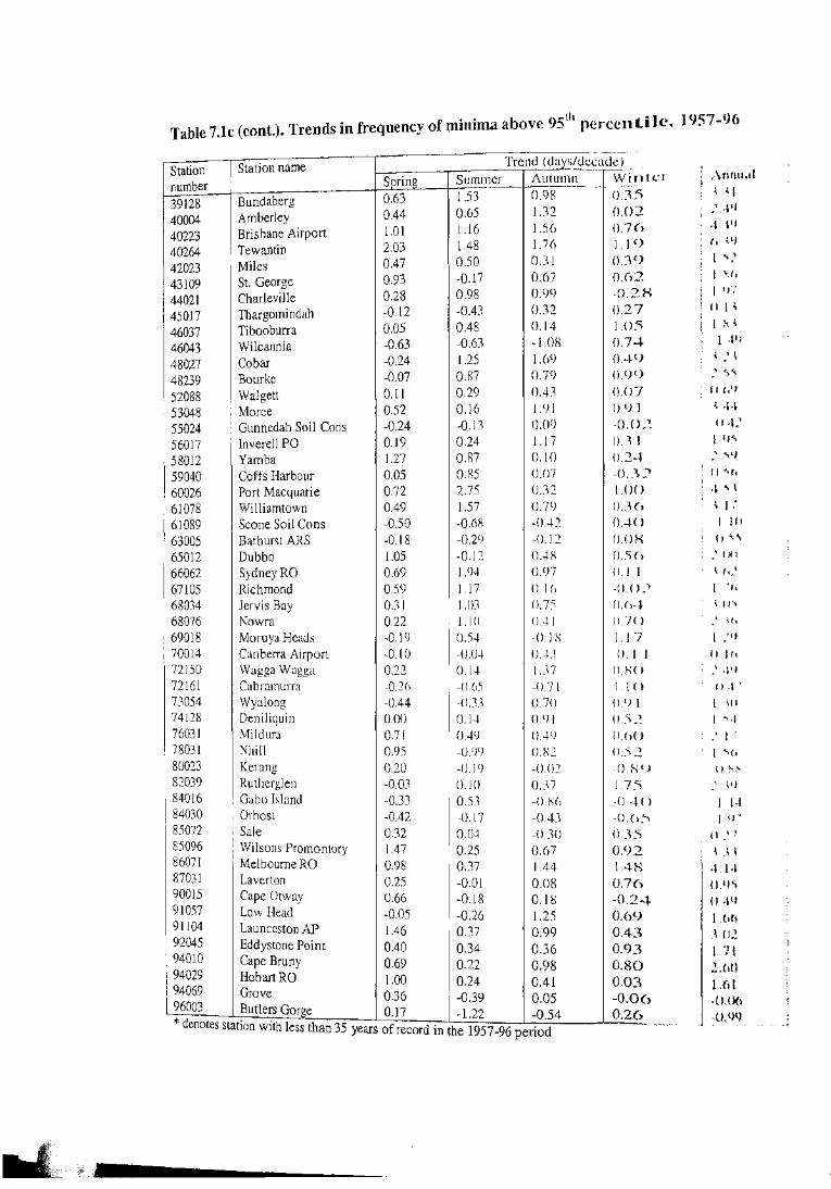
Table 7.1c (cont.). Trends in frequency of minima above 95th percen ti I e., 1957 .. 9(,
Station Station name number 39128 Bundaberg 40004 Amberley 40223 Brisbane Airport 40264 Tewantin 42023 Miles 43109 St. George 44021 Charleville 45017 Thargomindah 46037 Tibooburra 46043 Wilcannia 48027 Co bar 48239 Bourke 52088 Walgett 53048 Moree 55024 Gunnedah Soil Cons 56017 Inverell PO 58012 Yamba 59040 Coffs Harbour 60026 Port Macquarie 61078 Williamtown 61089 Scone Soil Cons 63005 Bathurst ARS 65012 Dubbo 66062 SydneyRO 67105 Richmond 68034 Jervis Bay 68076 Nowra 69018 Moruya Heads 70014 Canberra Airport 72150 Wagga Wagga 72161 Cabramurra 73054 Wyalong 74128 Deniliquin 76031 Mil dura 78031 Nhill 80023 Kerang 82039 Rutherglen 84016 Gabo Island 84030 Orbost 85072 Sale 85096 Wilsons Promontory 86071 Melbourne RO 87031 Laverton 90015 Cape Otway 91057 Low Head 91104 Launceston AP 92045 Eddystone Point 94010 Cape Bruny 94029 HobartRO 94069 Grove 96003 Butlers Gorge * denotes station with less than 35
Trend (days/d_~':_£lde) __
Spring Summer Autumn Winter --1-----------
0.63 1.53 0.98 0.35
0.44 0.65 1.32 0.02
1.01 1.16 1.56 0. 7 (l
2.03 1.48 1.76 1.1 C)
0.47 0.50 0.31 0.39
0.93 -0.17 0.67 0.(>2
0.28 0.98 0.99 -0.2X
-0.12 -0.43 0.32 0.27
0.05 0.48 0.14 1.05 -0.63 -0.63 -l.OR 0.74 -0.24 1.25 1.(19 0.4'J -0.07 0.87 0.79 (),C)C)
0.11 0.29 0.43 0.()7
0.52 0.16 1.91 0.9 1
-0.24 -0.13 0.09 -0. () 2 0.19 0.24 1.17 0.3 I 1.27 0.87 0.10 0.2A-0.05 0.85 0.07 -0 .. "\ :2 0.72 2.75 0.32 1.00 0.49 1.57 0.79 0 .. 1 (>
-0.50 -0.68 -0.42 0.4()
-0.18 -0.29 -0.12 0.0~
1.05 -0.12 0.4~ 0 .. '1 ()
0.69 1.94 o.<n 0. 1 1 0.59 1.17 0. I(> -0. () _:
0.31 I.()] 0. 75 () .( l•-l
0.22 1.10 0.41 0.7() -0.19 0.54 -0.1 K 1.17 -0.10 -0.04 (),4_) -0. I 1 0.22 0.14 1.37 0 _)-.;( ) -0.26 -0 .M -0.71 I. I 0 -0.44 -OJ.) 0.70 O.<J I 0.00 0.14 o.<J 1 0.)2 0.71 0.49 0.4 <) (),()()
0.95 -0.9() 0.~2 0.52 0.20 -0.19 -0.02 -0. :--; ()
-0.03 0.10 o.:n 1.7~
-0.33 0.53 -0.~(> -O.~l-< > -0.42 -0.17 -0.43 -0.(1:')
0.32 0.04 -0 . .30 0 .. 15 1.47 0.25 0.67 0.92 0.98 0.37 1.44 1.4H 0.25 -0.01 0.08 0.76 0.66 -0.18 0.18 -0.24 -0.05 -0.26 1.25 0.(>9 1.46 0.37 0.99 0.43 0.40 0.34 0.36 0.93 0.69 0.22 0.98 0.80 1.00 0.24 0.41 0.03 0.36 -0.39 0.05 -0.06 0.17 -1.22 -0.54 0.26
years of record m the 1957-96 penod
i \mm.d ~ q 1,&«J . t·&ll
( I \ ~)
1 .... ~~ 1 :!o\(t
I ( l. 1 ' l
~
~
n .),
1 ,$1)
.~ \
\~
l1 1)
I
.H l·L~
(J'\
\I)
\(,
.., \
I
' n ·l ~ l 1 IO (
) ..
' I
' I
I (I
I
(
I I I
l
l '"' on ( *;' 'fl
()'I
II
' I 1
()
~
·L 0. 0 1. J l. , L ~o
,()

Table 7.1d. Trends in frequency of minima above 90t11 percentile, 1957~96
Station Station name Trend (d~ys/decade) number Spring Summer Autumn Winter Annual 1021 Kalumburu 2.44 0.15 2.15 0.12 5.10 2012 Halls Creek -0.74 -1.69 -1.04 -2.36 -5.67 3003 Broome 3.87 1.33 -0.58 0.64 5.38 4032 Port Hedland 1.54 0.88 1.57 1.40 5.29 5007 Lear month -1.12 -6.18 -1.17 1.18 -5.92 5026 Wittenoom 0.20 0.38 0.78 0.64 2.06 6011 Carnarvon 1.01 1.50 0.21 1.45 4.30 7045 Meekatharra 0.46 0.24 0.50 0.49 1.53 8039 Dalwallinu 0.49 -0.89 -0.17 -0.53 -1.12 8051 Gerald ton 1.19 -0.78 1.19 0.65 2.19 9021 Perth Airport 3.01 1.58 1.81 0.66 6.85 9518 Cape Leeuwin 2.83 -0.48 1.35 2.47 6.22 9741 Albany 1.33 -0.24 2.25 1.54 4.68 9789 Esperance 1.35 1.48 1.45 1.12 5.41 10035 Cunderdin 0.82 -0.69 0.23 1.12 1.49 10648 Wandering 0.74 -0.84 -0.39 0.68 0.54 11052 Forrest 2.84 0.94 1.46 1.07 6.46 12038 Kalgoorlie 1.53 0.84 1.17 1.76 5.11 13017 Giles -0.56 1.05 0.36 -O.l7 0.76 14015 Darwin Airport 2.99 1.83 2.35 0.89 7.93 14825 Victoria River Downs* 2.60 0.14 3.18 -0.11 5.51 15135 Tennant Creek 0.33 1.53 2.82 1.23 5.94 15548 Rabbit Flat* 2.65 0.58 2.07 0.59 6.02 15590 Alice Springs 1.59 -0.13 -0.34 1.55 2.74 16001 Woomcra -0.60 -0.54 -0.25 2.26 1.07 16044 Tarcoola -0.24 1.91 1.08 -0.64 2.11 17031 Marrec -0.78 -0.24 l.lO -0.79 -0.65 17043 Oodnadatta -1.25 -1.22 -0.03 1.41 -1.13 18012 Ceduna 1.41 -0.40 0.97 0.66 2.54 18070 Port Lincoln 0.85 0.40 0.00 0.03 1.42
21046 Snow town 0.16 0.54 0.92 0.54 1.84 22801 Cape Borda 0.01 -0.61 0.23 0.77 0.53 23090 Adelaide RO 1.78 0.79 1.16 0.80 4.44
23373 Nuriootpa 1.06 0.48 1.75 1.50 4.89 2()021 Mount Gambier 2.70 1.25 2.29 2.13 8.18
26026 Robe 1.87 0.13 1.99 3.09 6.80 27022 Thursday Island 3.14 1.33 2.81 2.04 9.59
27045 Weipa 0.21 2.38 2.48 1.20 6.19
28004 Palmerville 2.59 -0.13 0.32 -0.28 2.73
29004 Burketown 1.68 2.96 3.59 1.98 10.00
30045 Richmond 2.28 2.91 2.01 1.62 8.79
31011 Cairns 3.68 2.34 5.02 2.97 13.94
32040 Townsville 2.02 3.06 2.54 1.97 9.55
33119 MackayMO 1.64 2.40 2.08 1.86 8.04
34084 Charters Towers 0.41 -0.14 1.65 1.27 3.36
36007 Barcaldine 1.56 3.12 2.39 0.57 7.93
36031 Longreach 1.13 1.60 3.59 1.64 7.90
37010 Camooweal 2.74 -0.19 -1.42 0.19 1.57
38002 Birdsville 0.01 0.20 0.31 -0.73 -0.05 38003 Boulia -0.78 -1.05 0.09 0.72 -1.00
39039 Gayndah 1.57 1.63 0.86 -0.37 3.65
39083 Rockhampton 1.15 1.84 2.85 0.85 6.75
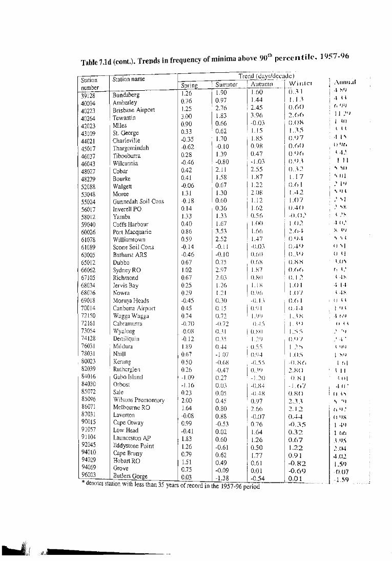
Table 7.1d (cont.). Trends in frequency of minima above 90th percentile .. 1957 .. t}(, __ ,______,__......____ .. ---
Station Station name Trend ( c.lays/dc~~l~C:L .
number Spring Summer Autumn Winter Anrm.;d
39128 Bundaberg 1.26 1.90 1.60 0.3 1 ·! SC)
40004 Amberley 0.76 0.97 1.44 1.13 •. ~ ~ \
40223 Brisbane Airport 1.25 2.76 2.45 (),()() (I tj!J
40264 Tewantin 3.00 1.83 3.96 2.()() ll2f»
42023 Miles 0.90 0.66 -0.03 0.( >H 1 tn
43109 St. George 0.33 0.62 1.15 1.35 ~n
44021 Charleville -0.35 1.70 1.85 o.<>7 ,, 1.~
45017 Thargomindah -0.62 -0.10 0.98 0.(>0 {! <J(l
46037 Tibooburra 0.28 1.39 0.47 o.<J<, LL'
46043 Wilcannia -0.46 -0.80 -1.03 o.<J J l l 1
48027 Co bar 0.42 2.11 2.55 0.32 ~-"0
48239 Bourke 0.41 1.58 un I. 17 "'\JJl
52088 Walgett -0.06 0.67 1.22 0.(> I •1 1'1
53048 Moree 1.31 1.30 2.08 ] . ..:~2 ."'t.«n
55024 Gunnedah Soil Cons -0.18 0.60 1.12 1.07 } '\l
56017 Inverell PO 0.14 0.36 1.()2 0.40 .' '~ 58012 Yamba 1.33 1.33 0.5(> -0.0.~ \ -·~"' 'If' f,lj
59040 Coffs Harbour 0.40 1.67 1.00 1.02 ,, n;~
60026 Port Macquarie 0.86 3.53 1.()() 2.(J··l \lJ
61078 Williamtown 0.59 2.52 1.47 0. <).t \ '\ :t
61089 Scone Soil Cons -0.14 -0.11 -o.cn OA<J {) 'll
63005 Bathurst ARS -0.46 -0.10 0.()() 0 .. ~<> () ~ l
65012 Dubbo 0.67 0.75 0.()8 O.XH UJ~
66062 SydneyRO 1.02 2.97 1.87 0.<><> (l ~}
67105 Richmond 0.67 2.03 0.80 0. J 2 \ ., s 68034 Jervis Bay 0.25 1.2() 1.18 1.01 ·l 1 .a 68076 Nowra 0.29 1.21 0. <)() 1.07 '.u-;, 69018 Moruya Heads -0.45 0.]0 -0.1.1 0 .(, I ll \ \
70014 Canberra Airport 0.45 0.15 0. <J I O.·l·l 1 .IJ 'i
72150 Wagga Wagga 0.74 0.72 I . <J <J l._q . .; I
• \ t,tJ
72161 Cabramurra -0.70 -0.72 -0 . ..J .'i l.Y> I I \ ~
73054 Wyalong -0.08 O.JI O.XO 1.~~ \ .'!J
74128 Deni1iquin -0.12 O.J.'l 1.2<) 0.'17 I -~ . 76031 Mil dura 1.89 0.44 () . .'i .') 1.2~ \ !tl)
78031 Nhill 0.67 -1.07 o.<J4 I.(>.~ 1 ;.;,q
80023 Kerang 0.50 -O.M~ -0 . .'15 -O.X(, 1 td 82039 Rutherg1en 0.26 -0.47 O.YJ 2.XO \ J I 84016 Gabo Island -1.09 0.27 -1.20 -0. X I :, ( ll 84030 Orbost -1.16 0.0] -0.04 -1.()7 .un 85072 Sale 0.23 0.05 -0.40 o.so () .~"' 85096 Wilsons Promontory 2.00 0.45 0.97 2.:~ :1 '\ N 86071 MelboumeRO 1.64 0.80 2.66 87031 Laverton
2.12 (lin
-0.08 0.88 -0.07 90015 Cape Otway
0.44 CIt) X
91057 0.99 -0.53 0.76 -0.35 I A'l
Low Head -0.41 0.02 91104 Launceston AP
1.64 0.32 1 ,(I{! 1.83 0.60
92045 Eddystone Point 1.26 0.67 .. \.'J~
1.26 -0.61 0.50 1.22 :~.04 94010 Cape Bruny 94029
0.79 0.62 1.77 0.9 1 .. U);! HobartRO 1.51 0.49 0.61 -0.82
94069 Grove 1.59
96003 0.75 -0.09 0.01 -0.69 "0.07 Butlers Gorge
* denotes station with less than 35 0.03 -1.38 -0.54 0.01 "1 .59
ears ofreco -Y rd m the 1957 96 pe110d

Table 7.1e. Trends in frequency of maxima below lOth percentile, 1957-96
Station Station name Trend (d[~ys/decade) number Spring Summer Autumn Winter Annual 1021 Kalumburu 2.39 0.33 -1.30 -0.84 0.82 2012 Halls Creek 0.08 0.70 0.21 -0.33 0.70 3003 Broome -1.23 0.95 -1.37 -2.68 -4.48 4032 Port Hedlund 0.59 -0.62 -0.67 -0.43 -1.01 5007 Learmonth -3.30 3.57 -1.24 1.76 -0.20 5026 Wittenoom -1.78 -0.02 0.13 -0.26 -1.35 6011 Carnarvon -0.09 0.67 -1.05 -0.26 -0.80 7045 Meekatharra 0.15 -0.54 -0.66 -0.34 -1.35 8039 Dalwallinu 0.11 -0.01 -1.18 -0.52 -1.47 8051 Geraldton -0.55 -0.78 -1.64 1.01 -2.05 9021 Perth Ai.rport -0.54 0.04 -1.26 0.36 -1.51 9518 Cape Leeuwin -0.70 0.93 -1.06 -0.59 -1.24 9741 Albany -0.55 1.58 -1.47 1.36 1.44 9789 Esperance -0.28 0.51 0.37 0.02 0.75 10035 Cunderdin -0.83 0.00 -2.09 -0.82 -3.53 10648 Wandering 0.24 0.34 -1.46 -0.33 -1.37 11052 Forrest -0.19 0.64 -1.08 -0.17 -0.80 12038 Kalgoorlie 0.18 1.03 -0.03 0.46 1.57 13017 Giles -0.66 0.03 0.25 -0.42 -0.88 14015 Darwin Airport -0.23 -1.12 -0.73 -1.87 -3.58 14825 Victoria River Downs* -1.12 -2.87 -1.58 -3.09 -7.68 15135 Tennant Creek 0.30 0.53 -0.26 -0.39 0.31 15548 Rabbit Flat* -4.31 -0.80 -2.04 -1.50 -9.18 15590 Alice Springs -0.30 -0.27 0.31 -0.36 -0.68 16001 Woomera 0.09 1.14 -0.98 1.64 2.34 16044 Tarcoola -1.30 0.29 -1.13 -1.95 -4.10 17031 Marrec -1.17 -0.25 -0.71 -1.92 -3.93 17043 Oodnadatta -0.71 0.33 -0.55 -2.44 -3.13 18012 Ceduna -1.04 -0.24 -1.27 -1.24 -3.84 18070 Port Lincoln -1.76 -1.90 -2.68 -2.19 -8.68 21046 Snowtown -1.24 -0.42 -1.38 -0.58 -2.75 22801 Cape Borda -2.24 -2.23 -1.71 -0.86 -7.12 23090 Adelaide RO -1.24 -0.73 -1.39 -0.78 -4.10 23373 Nuriootpa -0.62 0.11 -0.96 -0.76 -2.20 26021 Mount Gambier -1.29 -1.26 -1.5 I -0.21 -4.06 26026 Rohc -1.75 0.89 -1.31 -1.72 -3.96 27022 Thursday Island -2.62 -0.5 I -1.23 -2.44 -6.81
27045 Weipa -3.48 -0.92 -0.55 0.67 -4.26
28004 Palmcrvi lle 0.24 -1.25 -1.03 -0.26 -2.28 29004 Burketown 1.17 0.14 -2.42 1.39 -1.00
30045 Richmond 0.27 0.50 -3.07 0.05 -2.15
31011 Cairns -0.44 -0.01 -1.32 -1.28 -3.03
32040 Townsville -0.38 -0.42 -1.56 0.24 -2.23
33119 MackayMO 0.10 -2.15 -1.71 -0.01 -4.02
34084 Charters Towers -0.59 -2.24 -2.59 0.86 -4.54
36007 Barcaldine 0.45 -1.22 -1.15 0.81 -0.86
36031 Longreach 0.36 0.05 -0.47 0.35 0.15
37010 Camoowea1 ~0.84 0.15 -1.32 -0.65 -2.69
38002 Birds ville ~1.03 -0.81 -0.96 -1.43 -4.34
38003 Boulia -0.01 0.93 -0.83 -0.49 -0.68
39039 Gayndah -0.51 -1.71 -0.92 -1.25 -4.23
39083 Rockhampton 0.46 -1.80 -0.51 0.26 -1.55
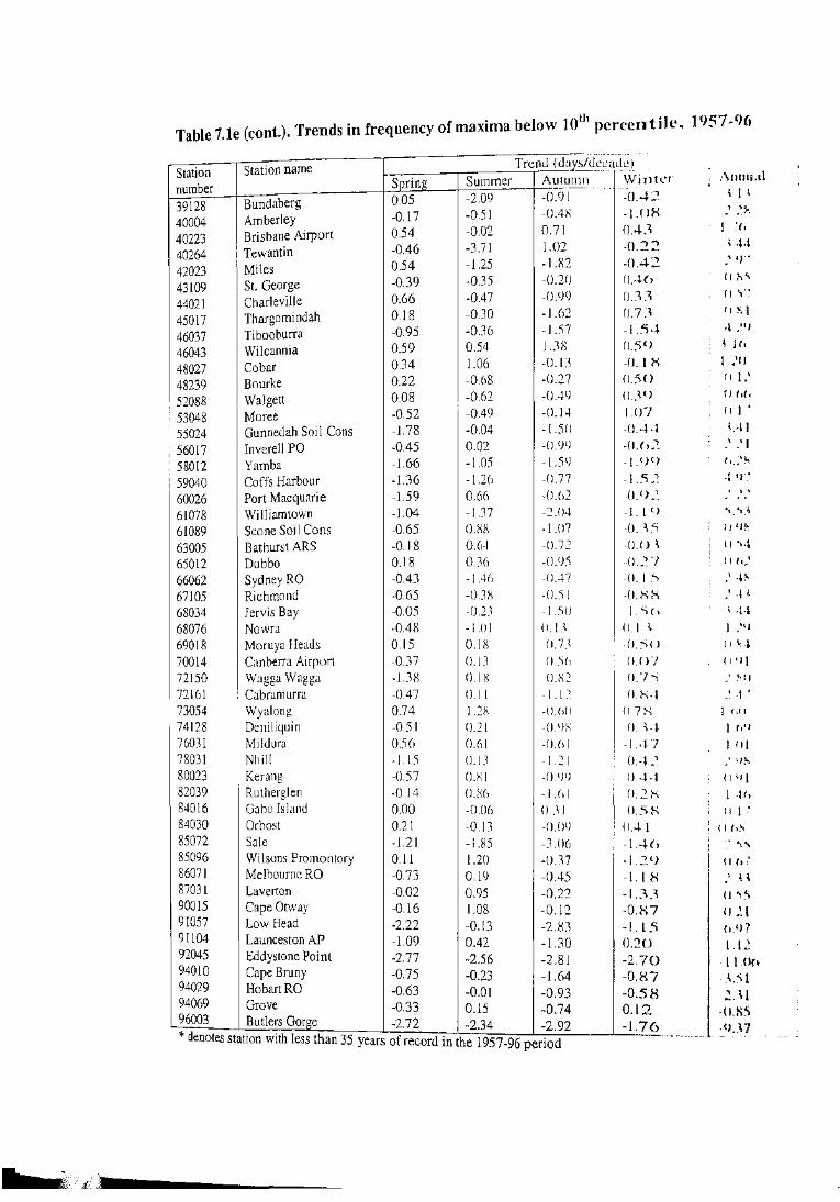
Table 7.1e (cont.). Trends in frequency of maxima below 1oth perccn tile., 1 '>S7 .. 96
~---.,--------,---------;:;:;--~---;-;-------~···· Station name Trend ( days/uccadeL Station
number Spring Summer Autumn WintL'f' ~~~-+-~-----~~~-~~~--~~~~----+·-~=
39128 Bundaberg 0.05 -2.09 -0.91 -0.4 2 40004 Amberley -0.17 -0.51 -0.4H -l.OH 40223 Brisbane Airport 0.54 -0.02 0.71 0.43 40264 Tewantin -0.46 -3.71 1.02 -0.2:2 42023 Miles 0.54 -1.25 -1.82 -0.4:?. 43109 St. George -0.39 -0.35 -0.20 (),..1.6
44021 Charleville 0.66 -0.47 -0.99 0.3 ~1 45017 Thargomindah 0.18 -0.30 -1.62 0.7 3 46037 Tibooburra -0.95 -0.36 -1.57 -1.:'14 46043 Wilcannia 0.59 0.54 1.38 ().~<) 48027 Co bar 0.34 1.06 -0. D -0. I H 48239 Bourke 0.22 -0.68 -0.27 0.50 52088 Walgett 0.08 -0.62 -0.4<) O.J<) 53048 Moree -0.52 -0.49 -0.14 1.07 55024 Gunnedah Soil Cons -1.78 -0.04 -1.50 -0.4~1 56017 Inverell PO -0.45 0.02 -0.9<J .. o.r,~: 58012 Yamba -1.66 -1.05 -l.S<J -1.()<) 59040 Coffs Harbour -1.36 -1.26 -0.77 -I.:') 2 60026 Port Macquarie -1.59 0.66 -0.(l2 .. o. () 4-,.
61078 Williamtown -1.04 -1.37 -2.04 -l.l<J 61089 Scone Soil Cons -0.65 0.88 -1.07 -0 .. ~ ~ 63005 BathurstARS -0.18 O.M -0.72 .(J.03 65012 Dubbo 0.18 OJ(> -0.()5 --0.27 66062 SydneyRO -0.43 -1.4(l -0.47 -0.1.'-l 67105 Richmond -0.65 -0.38 -0.51 -0. H s 68034 Jervis Bay -0.05 -0.23 -I .50 -I . ~ () 68076 Nowra -0.48 -1.01 O.D 0.1.~
69018 MoruyaHeads 0.15 O.IR -0.73 .(J.~()
70014 Canberra Airport -0.37 0.13 -0 .. '1(> -0.07 72150 Wagga Wagga -1.38 0.18 -(J.X2 -0.7 s 72161 Cabramurra -0.47 () II 1 1 1 · - . - 0. H·t 73054 Wyalong 0.74 1.28 -0.(>0 o. 7 s 74128 Deniliquin -0.51 0.21 -O.(Jr: o. ~·+ 76031 Mildura 0.56 O.(J 1 -O.(J 1 -I.·+ 7 78031 Nhill -1.15 () 11 . .1 - I . 2 I 0. ·-L~ 80023 Kerang -0.57 () o1 () <) . () - . <) -0 .4 . .t 82039 Rutherglen -0.14 0.8(> -!.(JI -0.2k 84016 Gabo Island 0.00 0 - . OCJ 0. J I -0. :'i k 84030 Orbost 0.21 0 - .13 -0.0<) 0.4 1 85072 Sale -1.21 1 85 8509
- . - -3.0(> -lA() 6 Wilsons Promontory 0.11 1 20 c ,
86071 . - L1 7 -I. :2 <>
Melbourne RO -0.73 0 8703
.19 -0.45 -I. l X 1 Laverton -0.02 0
90015 .95 -0.22 -1.3:"
Cape Otway -0.16 1.08 -0.12 -0.87 91057 Low Head -2.22 91104 L
-0.13 -2.83 -1.15 aunceston AP -1.09
92045 Edd P 0.42 -1.30 0.20
ystone oint -2.77 940
-2.5 6 -2.81 -2.7 () 10 Cape Bruny -0.75
9 -0.23 -1.64 -0.87
4029 Hobart RO _0.63 94069
-0.01 -0.93 -0.5 8' Grove -0.33
96003 B 1 G 0.15 -0.74 0.12
ut ers orge -2.72 *d -2.34 -2.92 -1.76 enotes station with less than 35 years of record 1·n the 1957-96 penod
AntHl!..;d
>iP , 2:k
l H1 ; ·l·~
~' tfl ()
1.1'n
{I ~ l ·l}tJ
' 1(1 1 •10 {I 1 I
{1ft(!
Ol
'" l .' .' I c.;'~
., '17
(I LJS
0 ').~
Cll!;1
.' ·!h } -t
·l·l l ;~~ J
r 1 h-i II ql ,' !",0
.• .r· 1 (.il I r.q I 111
: 111'\
1Jtq
1 ·H• II I
t I t1S ., "1'\
(Ui'.J' ~~ J -~
(J"\~
0 .21 (,,9'1
1 l1 . l 1 .fl<t -.\.:H --:;!. ;\ 1

Table 7.1f. Trends in frequency of maxima below 5th percentile, 1957-96
Station Station name Trend (days/decade) number Spring Summer Autumn Winter Annual 1021 Kalumhuru 1.35 -0.11 -1.09 -0.33 -0.03 2012 Halls Creek 0.25 0.52 0.25 -0.20 0.86 3003 Broome -0.75 0.25 -0.24 -1.59 -2.38 4032 Port Hedlund 0.14 -0.19 -0.02 0.13 0.11 5007 Lear month -1.71 1.84 -0.55 1.02 0.07 5026 Wittcnoorn -0.71 -0.01 0.30 -0.42 -0.32 6011 Carnarvon -0.38 -0.35 -0.69 0.02 -1.47 7045 Meekatharra 0.31 -0.43 -0.26 -0.28 -0.66 8039 Dalwallinu 0.02 -0.22 -0.75 -0.08 -0.85 8051 Gerald ton -0.27 -0.51 -0.89 0.96 -0.77 9021 Perth Airport -0.30 0.54 -0.59 0.60 0.19 9518 Cape Leeuwin -0.28 0.94 -0.92 -0.53 -0.70 9741 Albany -0.70 0.89 -0.85 0.46 0.21 9789 Esperance -0.35 0.13 0.05 0.07 0.04 10035 Cunderdin -0.38 -0.38 -1.25 -0.81 -2.75 10648 Wandering 0.17 0.36 -0.73 -0.10 -0.45 11052 Forrest 0.39 0.46 -0.50 -0.35 0.18 12038 Kalgr>Orlic 0.17 0.35 -0.08 0.40 0.82 13017 Giles -0.25 -0.03 0.03 -0.14 -0.35 14015 Darwin Airport 0.08 -0.53 -0.34 -0.70 -1.30 14825 Victoria River Downs* -1.11 -1.66 0.25 -1.51 -3.93 15135 Tennant Creek 0.03 0.58 0.18 -0.04 0.67 15548 Rabbit Flat* -2.12 -0.09 -1.21 -1.90 -5.81 15590 AI ice Springs -0.32 0.01 0.27 -0.18 -0.28 16001 Woomcra -0.41 1.07 -0.09 1.07 1.92 16044 Tarcoola -0.49 0.56 -0.80 -1.14 -l.98 17031 Marrec -0.62 -0.58 -0.59 -0.83 -2.56 17043 Oodnadatta -0.63 -0.08 -0.12 -1.18 -l.79 18012 Ceduna -0.47 -0.42 -0.40 -0.53 -l.88 18070 Port Lincoln -0.99 -1.31 -1.35 -1.54 -5.16 21046 Snow town -0.63 -0.27 -1.19 -0.38 -2.21 22801 Cape Borda -1.26 -1.35 -1.22 -0.67 -4.53 23090 Adelaide RO -0.76 -0.37 -0.83 -0.14 -2.13 23373 N u riootpa -0.57 -0.07 -0.51 -0.47 -1.59 2(J021 Mount Gambier -0.82 -0.37 -0.86 -0.22 -2.24
26026 Robe -1.29 0.71 -0.64 -0.74 -1.74 27022 Thursday Island -1.28 -0.49 -0.36 -1.36 -3.61
27045 Weipa -1.79 -0.22 0.37 0.08 -1.50 28004 Palmervillc 0.08 -0.69 -0.35 0.19 -0.80
29004 Burke town 0.32 0.10 -1.43 0.51 -0.97
30045 Richmond 0.29 0.42 -1.59 0.52 -0.34 31011 Cairns 0.20 0.21 -0.83 -1.08 -1.47
32040 Townsville -0.11 0.05 -0.57 0.63 -0.03 33119 MackayMO 0.09 -1.16 -0.68 0.40 -1.48
34084 Charters Towers -0.45 -1.01 -1.35 0.62 -2.11
36007 Barcaldine 0.09 -0.58 -0.46 0.79 -0.01
36031 Longreach 0.34 -0.13 -0.33 0.04 -0.04
37010 Camooweal -0.39 0.12 -0.70 -0.25 -1.29
38002 Birds ville -0.47 -0.27 -0.46 -0.90 -2.16
38003 Boulia 0.07 0.68 -0.37 0.43 0.62
39039 Gayndah 0.16 -1.20 -0.62 -0.91 -2.55
39083 Rockhampton 0.37 -0.86 0.23 -0.24 -0.44

Table 7.1f (cont.). Trends in frequency of maxima below 5th pcrcenti I c .. 1957-96 ~-·- ·-
Station Station name Trend ( days/deca~~l-
number Spring Summer Autumn Winter Amm.;~l
39128 Bunda berg 0.34 -1.53 -0.03 -0.:~ I 1 .•. ~(1
40004 Amberley 0.05 -0.25 0.17 -O.J9 n ·L~
40223 Brisbane Airport 0.33 0.05 0.33 0.07 0.1-!H
40264 Tewantin 0.65 -2.24 0.93 -0.73 1' l41
42023 Miles 0.41 -1.02 -0.92 -0.12 !.M1
43109 St. George -0.44 -0.23 -0.08 0.37 0 (;"'
44021 Charleville 0.11 -0.14 -0.(>2 0.25 0 ."\0
45017 Thargomindah 0.04 -0.42 -0.71 0.42 0 • .u, 46037 Tibooburra -0.32 -0.09 -0.92 -1. I'> ~~ .HJ
46043 Wilcannia 0.26 0.22 1.49 0.42 ~~ 40
48027 Co bar 0.01 0.49 -0.31 -0.:2~+ (Jf)\
48239 Bourke 0.03 -0.59 0.39 ··0.:27 11'\l
52088 Walgett 0.19 -0.41 -0.23 -O.C )5 IUt~~
53048 Moree -0.33 -0.24 -0.14 0.(>6 rUt<J
55024 Gunnedah Soil Cons -0.88 -0.14 -0.(>(> -0.4H =~ .0~'
56017 Inverell PO -0.45 0.20 -0.52 -0.43 1:~~
58012 Yamba -0.78 -0.13 -1.0 I -0. <)() } sc. 59040 Coffs Harbour -0.59 -0.49 -0.30 -1.05 .~ :'\ 1 60026 Port Macquarie -0.62 0.67 -0.1 (> -0.5 ~ Cl. ·~
61078 Williamtown -0.45 -0.83 -1.15 -0.<)(, ~.·L'
61089 Scone Soil Cons -0.23 0.06 -1.02 .. ().05 1 t~l 63005 Bathurst ARS 0.03 0.17 -0.54 0.4.() II UH
65012 Dubbo 0.26 -0.2(> -0.5 (> (). l () ll \.l
66062 Sydney RO -0.28 -0.74 -0. I X .. (). 1 ( ) 1 HJ 67105 Richmond -0.29 O.OH O.OX -O .. H) () .t ' 68034 Jervis Bay -0.10 -0.70 -0.57 -O.H<> .' l"i 68076 Nowra 0.12 -0.0 I O.(l> 0.5.~ 1 q 69018 Moruya Heads 0.31 (). ]<) -0.10 0.0 I 0 "'\ 70014 Canberra Airport 0.04 0.37 -0. I 7 -0. I l I) II.'
72150 Wagga Wagga -0.85 0.11 -0.(>) -0. I q 1 r. I 72161 Cahramurra -0.38 0.3(> -0.50 0.:'1 ~ l 1'1 73054 Wyalong 0.08 (). <)4 -0.4 7 0.7·l 1 I 1 74128 Deniliquin -0.85 0.(>2 (),()<) O .. H > ( 1 I ' 76031 Mil dura 0.30 0.38 -0.3 7 .() .•l . J, () }fl 78031 Nhill -0.66 0.18 -0 . ..:14 0.2 . .: (I ;.H1 80023 Kerang -0.22 -0.17 -0.4X 0.2·-l- (I \(, 82039 Rutherglen -0.74 0.10 -0.93 -0. I 1 J IJl 84016 Gabo Island -0.36 0.05 0.5X -0. l H O.!IJ 84030 Orbost 0.32 0.04 0.22 -0.()·-· (I .' 85072 Sale -0.71 -0.6CJ -1.20 -0.()() 85096 l, .' '
86071 Wilsons Promontory -0.46 0.34 -0.4X -0.()4 I ~c, Melbourne RO -0.68 0.22 -0.31 -0 . .17
87031 1 p; Laverton -0.47 0.73 -0.09 -0.6H
90015 {t:'\0
91057 Cape Otway -0.08 0.94 0.05 -0.2 <) ().;'\t1 Low Head -1.82 0.30 -1.76 -O.HO
91104 ·k:'\0
92045 Launceston AP -0.82 0.28 -1.22 -O.OH 1.~0
94010 Eddystone Point -1.26 -1.44 -1.93 -2.05 -(d\0
94029 Cape Bruny -0.38 -0.46 -1.14 -1.56 ",,,:"i()
94069 HobartRO -0.56 0.12 -0.74 -0.34 ~ l.{\4 Grove -0.42 0.10 -0.72 0.13 $0,91 ~6003 Butlers Gorge -1.84 -1.76 -1.79 -0.79 -Cl.:r\ * denotes station with les s than 35 years of record m the 1957-96 penod
n ·z
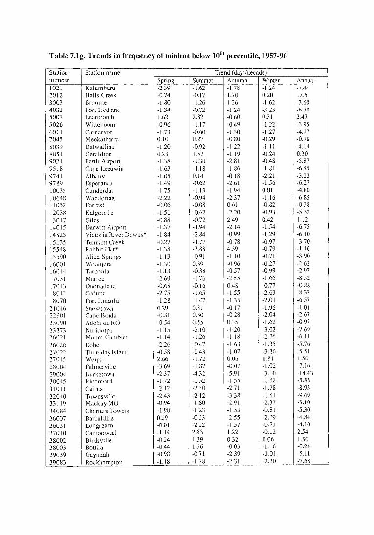
Table 7.1g. Trends in frequency of minima below lOth percentile, 1957-96
Station Station name Trend (days/decade) number Spring Summer Autumn Winter Annual 1021 Kalumburu -2.39 -1.62 -1.78 -1.24 -7.44 2012 Halls Creek -0.74 -0.17 1.70 0.20 1.05 3003 Broome -1.80 -1.26 1.26 -1.62 -3.60 4032 Port Hedland -1.34 -0.72 -1.24 -3.23 -6.70 5007 Learmonth 1.62 2.82 -0.60 0.31 3.47 5026 Wittcnoom -0.96 -1.17 -0.49 -1.22 -3.95 6011 Carnarvon -1.73 -0.60 -1.30 -1.27 -4.97 7045 Meekatharra 0.10 0.27 -0.80 -0.29 -0.78 8039 Dalwallinu -1.20 -0.92 -1.22 -1.11 -4.14 8051 Gerald ton 0.23 1.52 -1.19 -0.24 0.30 9021 Perth Airport -1.38 -1.30 -2.81 -0.48 -5.87 9518 Cape Leeuwin -1.63 -1.18 -1.86 -1.81 -6.45 9741 Albany -1.05 0.14 -0.18 -2.21 -3.23 9789 Esperance -1.49 -0.62 -2.61 -1.56 -6.27 10035 Cunderdin -1.75 -1.13 -1.94 0.01 -4.80 10648 Wandering -2.22 -0.94 -2.37 -1.16 -6.85 11052 Forrest -0.06 -0.08 0.61 -0.82 -0.38 12038 Kalgoorlie -1.51 -0.67 -2.20 -0.93 -5.32 13017 Giles -0.88 -0.72 2.49 0.42 1.12 14015 Darwin Airport -1.37 -1.94 -2.14 -1.54 -6.75 14825 Victoria River Downs* -l.84 -2.84 -0.99 -1.29 -6.10 15135 Tennant Creek -0.27 -1.77 -0.78 -0.97 -3.70 15548 Rabbit Flat* -1.38 -3.88 4.39 -0.79 -1.16 15590 Alice Springs -1.13 -0.91 -1.10 -0.71 -3.90 16001 Woomcra -1.30 0.39 -0.96 -0.27 -2.62 1 ()()44 Tarcoola -1.13 -0.38 -0.57 -0.99 -2.97 17031 Marn~c -2.69 -1.76 -2.55 -1.66 -8.52 17043 Oodnadatta -0.68 -0.16 0.48 -0.77 -0.88 18012 Ceduna -2.75 -1.65 -1.55 -2.63 -8.32 18070 Port Li nco) n -1.28 -1.47 -1.35 -2.01 -6.57 21046 Snow town 0.29 0.31 -0.17 -1.96 -1.01 22801 Cape Borda -0.81 0.30 -0.28 -2.04 -2.67 23090 Adelaide RO -0.54 0.55 0.35 -1.62 -0.97
23373 Nuriootpa -1.15 -2.10 -1.20 -3.02 -7.69 2(>021 Mount Gamhicr -1.14 -1.26 -1.18 -2.76 -6.11 2()02() Rohe -2.26 -0.47 -1.63 -1.35 -5.76 27022 Thursday IslanJ -0.58 -0.43 -1.07 -3.26 -5.51
27045 Weipa 2.66 -1.72 0.06 0.84 1.50 28004 Palmcrvillc -3.69 -1.87 -0.07 -1.02 -7.16
29004 Burketown -2.37 -4.32 -5.91 -3.10 -14.43
30045 Ridm1oml -1.72 -1.32 -1.55 -1.62 -5.83
31011 Cairns -2.12 -2.30 -2.71 -1.78 -8.93
32040 Townsville -2.43 -2.12 -3.38 -1.61 -9.69
33119 MackayMO -0.94 -1.80 -2.91 -2.37 -8.10
34084 Churters Towers -1.90 -1.23 -1.53 -0.81 -5.30
36007 Barcaldine 0.29 -0.13 -2.55 -2.29 -4.84
36031 Longreach -0.01 -2.12 -1.37 -0.71 -4.10
37010 Camooweal -1.14 2.83 1.22 -0.12 2.54
38002 Birdsville -0.24 1.39 0.32 0.06 1.50
38003 Boulia -0.44 1.56 -0.03 -1.16 -0.24
39039 Gayndah -0.98 -0.71 -2.39 -1.01 -5.11
39083 Rockhampton -1.18 -1.78 -2.31 -2.30 -7.68

'fable 7.1g (cont.). Trends in frequency of minima below IO'h pereentile, 1957-96
Station Station name J----,-----T_re...,.·n __ d_;_( u_ayE~}~~c a de J
number Spring Summer Autumn Winter ~ Bundaberg -0.34 -1.89 -2.31 l.H(,
400o4 Amberley -0.76 -0.97 -1.44 -·I. 13
40223 Brisbane Airport -1.85 -2.52 -2.9K -2.Ml
40264 Tewantin -3.12 -2.56 -3.70 <1.(U
42023 Miles 0.29 -0.67 -0.92 1 ..tO
431o9 St. George -0.47 -0.75 -0.64 J .I<)
44021 Charleville -2.03 -1.04 -0.91 -2.30
45017 Thargomindah -1.26 -2.12 -0.33 1 AX
46037 Tibooburra -0.94 -0.42 -0.17 0.4 J
46043 Wilcannia 0.59 2.96 1.RC> 0.07
48o27 Co bar -2.67 1.09 -O.K7 1. 7 ~
48239 Bourke -0.76 -0.86 -0.70 .J.(1<)
52088 Walgett -1.16 -0.10 -1.14 o.Tl
53o48 Moree -2.75 -2.17 -2.01 \.,~<)
55024 Gunnedah Soil Cons -0.72 -0.15 -0.(>2 1 AO
56017 Inverell PO -1.70 -1.23 .().<)i{ 2.77
58012 Yamba -1.07 -0.89 -1.34 o.<rJ
59040 Coffs Harbour -1.34 -2.21 -2.<)() .:. 70
60026 Port Macquarie -2.86 -2.61 -3.34 .~.·-~<)
61078 Williamtown -0.35 0.12 -J.KR l.W)
61089 SconeSoiiCons 1.11 0.65 -0.14 .(JAO
630o5 Bathurst ARS 0.26 0.98 -ru:o J.cd 65012 Dubbo -0.17 -O.O(J -1.10 1.7.:
66062 SydneyRO -0.30 -1.04 -O.CJC> !Uri 67105 Richmond 1.34 -0.32 -0.07 (J. H·t
68034 Jervis Bay -0.4 7 0.12 -O.(><) () 1 '/
68076 Nowra 0.88 -0.57 -run !J .. l'/ 69018 Moruya Heads -0.70 0.18 -O.(>.~
C b A' !.OS 70014 an erra 1rport -1.62 -1.13 .J.<)2 1 ( s 72150 Wagga Wagga -1.00 1 51 ·· )I Cb --- -1.1.~ !J.().l 72161 a ramurra -0.10 0.50 -0.40 () ')')
73054 Wyalong -0.44 0 6'1 -(J.I-'(J .• 1 () () ( )<)
74 128 Deniliquin -0.01 -0.37 -(J~l (JJI
031 Mildura 1 75 ·· .l · 76 -.- -1.53 1.72 1.11
78031 Nhill 0.57 1.31 -O.<JO () '·') 80023 Kerang 0.44 -0.59 0.4X o. 7.2 82039 Rutherglen 0.69 2.34 O.R4 O.<J<)
84016 Gabo Island 0.27 0.1() -(J. ,, 1 0 b '+ ()_ . .j.() 84030 r ost 0.54 -0.61 1
72 Sale J3 O.H:'i
850 -0.45 -1.48 w·I p -O.R2 1.7 3 85096 1 sons romontory -1.40 _1_94 86071 Melbourne RO -1.47 -1. 18 -
3.64 -1.9.'1
87031 Laverton 0 -1.19 -I A4
·23 -1.08 I 5:1 90015 CapeOtway _1_93 1.51 -... -0.92
L H -2.27 () <J7
91057 ow ead -0.59 1.37 ... 91104 Launceston AP -1.95 _2.73 -0.15 -0.52 92045 EddystonePoint -1.80 _1.04 -l.09 -1.3H
C B -1.94 -1.4S 94010 ape runy -1.53 -0.97
94029 HobartRO -1.57 -0.39
-1.35 -1.23 94069 Grove -0.74 -0 22 -1.77 -0.71 96003 Butlers Gorge -0.11 O 0· -1.40 -1.00
L..--:-:"" . 'th 1 ' 0 -0.31 ) *denotes statiOn WI ess than 35 years of record in the 1957-96 penod C .78
---------------------~
AnmMf (I I ·1 n liU 11.1\ } .~rj
t ;~ ~
(,}'
.tl'\4
.l rn .a 'il ·l ,, ;' .~ q HI! to :'n ~. ~fh
tdl,!
·1 Hj tl ,1 0
11.1 Sli
\ ~ '{
{) "" (I 1) 11
.It)/
{ I~ ()\I
1 td, ,, .l(,
' l r J .~ (,IJ)',
I I"~
II'"!(,
I td I I 'I (I ()lj
() c,o () 1)11
.' l)"l
u .'I 1 .tl(l 0. N q_ \.l
·.'\.OS 2.7~
~~ .1 ~ ·0.11 .. (,J.;.t
.(,,C)I)
····~.H5 ··5.10 <"t46 0.09
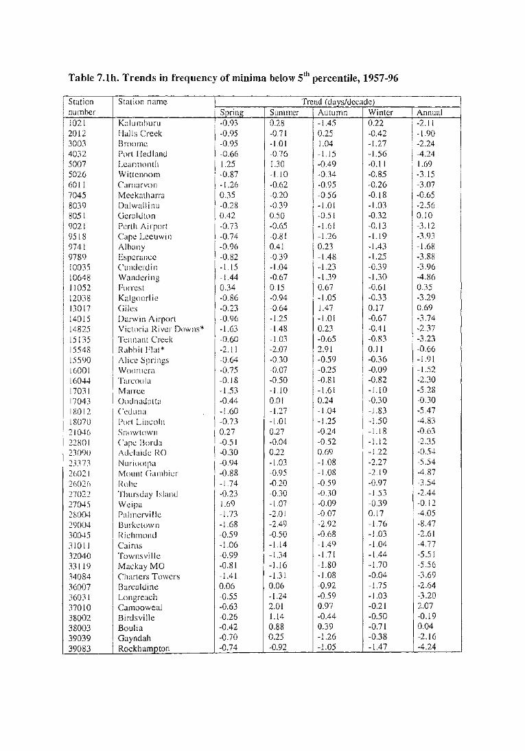
Table 7.1h. Trends in frequency of minima below 5t11 percentile, 1957-96
Station Station name Trend (days/decade) number Spring Summer Autumn Winter Annual 1021 Kalumburu -0.93 0.28 -1.45 0.22 -2.11 2012 Halls Creek -0.95 -0.71 0.25 -0.42 -1.90 3003 Broome -0.95 -1.01 1.04 -1.27 -2.24 4032 Port Hed land -0.66 -0.76 -1.15 -1.56 -4.24 5007 Learmonth 1.25 1.30 -0.49 -0.11 1.69 5026 Wittenoom -0.87 -1.10 -0.34 -0.85 -3.15 6011 Carnarvon -1.26 -0.62 -0.95 -0.26 -3.07 7045 Meekatharra 0.35 -0.20 -0.56 -0.18 -0.65 8039 Dalwalli nu -0.28 -0.39 -1.01 -1.03 -2.56 8051 Gerald ton 0.42 0.50 -0.51 -0.32 0.10 9021 Perth Airport -0.73 -0.65 -1.61 -0.13 -3.12 9518 Cape Leeuwin -0.74 -0.81 -1.26 -1.19 -3.93 9741 Albany -0.96 0.41 0.23 -1.43 -1.()8 9789 Esperance -0.82 -0.39 -1.48 -1.25 -3.88 10035 Cundcrd in -1.15 -1.04 -1.23 -0.39 -3.96 10648 Wandering -1.44 -0.67 -1.39 -1.30 -4.86 11052 Forrest 0.34 0.15 0.67 -0.61 0.35 12038 Kalgoorlic -0.86 -0.94 -1.05 -0.33 -3.29 13017 Giles -0.23 -0.64 1.47 0.17 0.69 14015 Darwin Airport -0.96 -1.25 -1.01 -0.67 -3.74 14825 Victoria River Downs* -1.63 -1.48 0.23 -0.41 -2.37 15135 Tennant Creek -0.60 -1.03 -0.65 -0.83 -3.23 15548 Rahhit P'lat* -2.11 -2.07 2.91 0.11 -0.66 15590 Alice Springs -0.64 -0.30 -0.59 -0.36 -1.91 16001 Woornera -0.75 -0.07 -0.25 -0.09 -1.52 J(J044 Tare nola -0.18 -0.50 -0.81 -0.82 -2.30 17031 Marrec -1.53 -1.10 -1.61 -1.10 -5.28 17043 Oodnadatta -0.44 0.01 0.24 -0.30 -0.30 18012 Ceduna -1.60 -1.27 -1.04 -1.83 -5.47 18070 Port Lincoln -0.73 -1.01 -1.25 -1.50 -4.83 2104Cl Snow town 0.27 0.27 -0.24 -1.18 -0.63 22801 Cape Borda -0.51 -0.04 -0.52 -1.12 -2.35 23090 Adelaide RO -0.30 0.22 0.()9 -1.22 -0.54 23373 NuriO(l!pa -0.94 -1.03 -1.08 -2.27 -5.54 2CJ021 Mount Gambier -0.88 -0.95 -1.08 -2.19 -4.87 2CJ02Cl Robe -1.74 -0.20 -0.59 -0.97 -3.54 27022 Thursday Island -0.23 -0.30 -0.30 -1.53 -2.44 27045 Weipa 1.69 -1.07 -0.09 -0.39 -0.12 28004 Palmervi lie -1.73 -2.01 -0.07 0.17 -4.05 29004 l3urketown -1.68 -2.49 -2.92 -1.76 -8.47 30045 Richmond -0.59 -0.50 -0.68 -1.03 -2.61
31011 Cairns -1.06 -1.14 -1.49 -1.04 -4.77
32040 Townsville -0.99 -1.34 -1.71 -1.44 -5.51 33119 Mackay MO -0.81 -1.16 -1.80 -1.70 -5.56
34084 Charters Towers -1.41 -1.31 -1.08 -0.04 -3.69
36007 Barcaldine 0.06 0.06 -0.92 -1.75 -2.64
36031 Longreach -0.55 -1.24 -0.59 -1.03 -3.20
37010 Camooweal -0.63 2.01 0.97 -0.21 2.07
38002 Birds ville -0.26 1.14 -0.44 -0.50 -0.19
38003 Boulia -0.42 0.88 0.39 -0.71 0.04
39039 Gayndah -0.70 0.25 -1.26 -0.38 -2.16
39083 Rockhampton -0.74 -0.92 -1.05 -1.47 -4.24

Table 7.1h (cont.). Trends in frequency of minima bcl<nv 5t11
percentile, 1957 -•J6
Station Station name Trend (days/deL' adt• I ~------~-------,----·····
number Spring Summer Autumn \\'mtcr ~~=-~----------------~~~--~~~---~--~·-:
39128 Bundaberg -0.58 -1.03 -1.02 l.l' 40004 Amber ley -0.43 -0.11 -0.40 40223 Brisbane Airport -0.94 -1.56 -1 .44 40264 Tewantin -2.68 -1.84 -1.77 42023 Miles -0.34 0.23 43109 St. George -0.56 -0.50 44021 Charleville -0.92 -0.56 45017 Thargomindah -0.58 -1.37 46037 Tibooburra -0.58 -0.12 46043 Wilcannia 0.64 1.50 48027 Cobar -1.46 0.54 48239 Bourke -0.55 52088 Walgett -1.18 53048 Moree -1.80 55024 Gunnedah Soil Cons -0.92 56017 Inverell PO -0.88 58012 Yamba -0.79 59040 Coffs Harbour -0.77 60026 Port Macquarie -1.36 61078 Williamtown -1.58 61089 Scone Soil Cons 0.43 63005 Bathurst ARS 0.15 65012 Dubbo 0.01 66062 Sydney RO -0.24 67105 Richmond 0.97 68034 Jervis Bay -0.17 68076 Nowra 0.85 69018 Moruya Heads -0.51 70014 Canberra Airport -0.67 72150 Wagga Wagga -0.58 72161 Cabramurra -0.08 73054 Wyalong -0.17 74128 Deniliquin -0.18 76031 Mildura -1.27 78031 Nhill -0.01
-0.36 0.04 -0.58 -0.46 -0.60 -0.48 -1.64 -1.53 -0.1 () 0.68 0.97 0.48 -0.49 0.04 0.38 ().] 8 0.38 -0.57 0.72 -0.02 -OJ.~
-0.4(1 -1.07 1.2(1
80023 Kerang 0.27 -0.1 (1
0.22 0. ()()
.(),()<)
-0.20 1.07 -O.:W
-O.C1 I -1 .. 1<)
-0.2.~
-OAC1 -I.CJH -1.7·+ -0. 7H -0.4(1 -0.71 -0.77
0.0) -O.OS -0.7) -1.2<J -OJJ l -0.()7 -O .. "l2 -0.2()
-1.07 -O.·U
82039 Rutherglen -0. 18 84016 Gabo Island 0 1.07 O.H<l
84030 .12 0.03 0.1 l
Orbost 0 26 85072 Sale . 0.37 O.HX
8 0.36 -1.04 -0.5<)
5096 Wilsons Promontory -0.91 86071 Melbourne RO -0.83 -1.23 -I.X5 87031 Laverton -0.56 -0.(1(1
90015 Cape Otway ~o~go -0.68 -0.6X 91057 Low Head -0.78 0.55 -1.50 91104 L 1.47 0.07 aunceston AP _1.24 92045 Eddystone Point -1.31 -
1.4
1 -0.62
94010 Cape Bruny -0.46 -0.90 94029 HobartRO -1.22 -0.61 -1.05 94069 -1.27 -0.69 -1.16 Grove _0.76 :6003 ~utlers Gorge 0.42 ~~:~~ -0.99
denotes statiOn with less than 35 years of record. -0.26 m the 1957-96 penod
()_.l)
I.JI) 2.1 () 1.1 .1.
O.H<J
J .• n cun
0.07 I () •H)
I ,.t.J l.!J)
() ')(,
I.H~
II} l.S'/ () '. ~ 1 I . ( ,q
IAI 2 ()(, ()( ).f
l .• 1 H I fl.,
(),l}
(},f()
().H)
( )( )_\
c Ul I I\.)
() s l () ()(,
() l·l () .l :--;
!l I "1
()(){)
( J ()X
() l () (Jr/
( J.( )•-~
(), ( l.~
.(). () ··~
-O.X2 ·O .• Y> "(), 7 -~ ~o.ox
"(), 74 ··0.5:2 m(),55 ~0.33
~0.60
0.48
Annu;d \ (;f<',
1 " ~ ~
(I 00
091 1 ~~~ \
.' \
0 -~ .,~
, 1
;''J. } ·ll ., ';
~.11:>
~
.' 1 4
·' s i ';, '
•l 4 I
(I rt;\
fJ ,:.;, 1 I lO
I"'' ll I l
I I \(,
I 11"1
II tf'
' II ;I 1 rH ll .1fl
1 t.' C I '1 •
·l (I /
I () s • () .' .' I 'II
CJU
} Ill
U.'·~
". l." .:.xo (},<)7
J_t)~
().(}\
.t·n :t76 ~3.7(1
<t47 -2.55 0.62

Table 7.2a. Trends in frequency of maxima above 30°C, 1957~96
Station Station name Trend (days/decade) Mean number Spring Summer Autumn Winter Annual annual
days > 30°C
1021 Kalumburu 0.28 1.52 1.58 3.11 339.9 2012 Halls Creek -0.22 -1.23 -0.27 -2.25 279.9 3003 Broome 0.40 0.14 1.47 4.27 6.27 273.2 4032 Port Hedland 0.14 0.56 1.62 2.46 263.9 5007 Learmonth 4.38 2.78 10.78 212.7 5026 Wittenoom 1.38 0.52 0.74 1.87 234.2 6011 Carnarvon -1.99 0.53 2.56 1.14 94.3 7045 Meekatharra 0.11 0.45 0.84 0.54 168.8 8039 Dalwallinu -0.11 -0.15 0.75 0.42 120.4 8051 Gerald ton -0.08 -0.02 1.88 1.76 81.1 9021 Perth Airport 0.02 0.93 1.33 1.82 72.0 9518 Cape Lccuwin 0.20 0.26 3.5 9741 Albany -1.86 0.73 -1.99 18.3 9789 Esperance -0.26 -3.25 -1.05 -4.59 37.4 10035 Cundcrdin 0.36 0.29 1.30 1.66 97.7 10648 Wandering -0.57 -1.62 0.12 -2.00 75.8 11052 Forrest -0.16 -0.42 0.08 -0.30 98.2 12038 Kalgoorlie 0.03 -0.02 -0.23 -0.39 103.9 13017 Giles 1.65 0.02 -0.29 1.59 182.9 14015 Darwin Airport 1.19 1.01 2.56 4.50 320.2 14825 Victoria R. Downs* 0.35 3.81 8.39 305.5 15135 Tennant Creek 0.26 -0.41 1.36 1.40 234.4 15548 Rabbit Flat* 2.26 -0.11 5.17 4.68 I 0.91 259.3 15590 Alice Springs 1.52 0.48 -0.09 2.67 172.6 16001 Woomera -0.97 -3.41 -2.78 -8.75 117.1 16044 Tarcoola 0.93 0.29 0.49 2.34 129.2 17031 Marrec 0.84 0.89 -1.27 0.46 164.0 17043 Oodnadatta 0.90 0.22 0.22 0.05 165.1 18012 Ceduna -0.13 -0.13 -0.31 -0.66 60.7 18070 Port Li nco! n -0.10 0.03 -0.23 -0.28 21.1 2104(l Snowtown 0.55 1.67 0.14 0.60 71.5 22801 Cape Borda -0.46 -0.34 9.6 23090 Adelaiue RO 0.06 0.95 0.33 1.06 50.5 23373 Nuriootpa -0.11 -0.10 0.74 0.62 48.8 2(J021 Mt Gambier -0.22 -0.19 0.25 -0.37 25.0 26026 Robe -0.35 -0.14 7.0 27022 Thursday Islanu 4.97 3.72 3.47 12.42 128.1 27045 Weipa 2.12 1.23 -1.40 2.91 322.4
28004 Palmcrville 0.68 0.81 1.79 3.21 318.5 29004 Burkctown -0.84 -0.51 1.58 -1.81 0.38 285.2
30045 Richmond -0.17 -0.26 2.95 O.O(J 3.10 261.6 31011 Cairns 2.38 -0.18 1.39 3.61 142.4 32040 Townsville 2.42 3.14 7.75 13.42 142.7 33119 Mackay MO 3.54 6.74 1.42 12.13 57.8 34084 Charters Towers 0.16 2.25 3.91 0.03 6.88 192.5 36007 Barcaldine -0.04 0.42 2.65 2.33 196.9 36031 Long reach -0.29 0.97 -0.12 0.38 217.1
37010 Camoowea1 0.28 0.19 3.35 3.88 259.5 38002 Birds ville 0.89 0.19 -0.59 1.34 2.01 197.4
38003 Boulia 0.87 1.81 1.22 3.40 215.9

Table 7.2a (cont.). Trends in frequency of maxima above 30°C, 1957-96 -. ~-·~--_,___., ..
Station Station name Trend (days/decade) --·-~ ~··--~·---
Mean number Spring Summer Autumn Winter Annual annual
days > 30°C -------
39039 Gayndah 2.67 2.85 1.94 7.25 134.1
39083 Rockhampton 1.30 3.78 0.97 5.R2 131.9
39128 Bundaberg 0.64 4.99 1.17 6.3R 49.6
40004 Amberley 1.97 1.70 -0.16 3.43 90.4
40223 Brisbane Airport 0.24 -1.33 -1.05 -2.05 36.5
40264 Tewantin 1.65 4.27 -0.36 5.13 35.1
42023 Miles 1.47 3.27 1.55 5.95 127.9
43109 St. George 1.39 0.27 0.02 2.12 148.3
44021 Charleville 0.08 0.47 0.93 2.35 155.3
45017 Thargo mi ndah 0.32 0.91 2.52 4.0(> 164.7
46037 Tibooburra 0.83 0.91 -0.96 (),C) X 145.3 46043 Wilcannia 0.38 0.84 -1.02 0.31 128.6 48027 Co bar -0.04 -1.40 -0.74 -2.17 108.2 48239 Bourke 0.69 1.45 -0.26 2.23 141.7 52088 Walgett -0.17 0.65 0.42 o.ox 13(>.2 53048 Moree 0.71 O.RO -0.51 1.14 115.5 55024 Gunnedah Soil Cons 0.03 1.59 -1.42 -0.4() xx.o 56017 lnverell PO 0.61 3J6 0.20 3.49 (){),()
58012 Yamba 0.1 C) 1.0 1 (),3
59040 Coffs Harbour 0.22 (),()() OAl 13.1 61078 Williamtown 0.43 1.02 -0.42 1.22 3(>.5 61089 Scone Soil Cons -1.30 1.1 () -2.X2 -3.Cd (>(),()
63005 Bathurst ARS 1.2(> O.XC> 29.4 65012 Duhho -0 . .81 0.15 -0. I 3 -I. I I 87.3 66062 Sydney RO -0.42 -0.03 -0.55 -I .00 15.0 67105 Richmond -0.23 -0.14 -0.75 -(}.-~() 55.0 68034 Jervis Bay -0 .. 13 -OAH Cl.H 68076 Nowra 0.14 (J.(J7 -0.42 0.0 I 23.1 (J9018 Moruya I !calls -O.OX 0.0:1 (1.5
70014 Canhcrra Airport ().)() 0. I 5 2CJ .4 72150 Wagga Wagga -O.C17 1.14 -0. IC1 -0.07 (14.2 73054 Wyalong 0.2X -1.22 -I.X2 -I.J4 X0.2 74128 Dcniliquin -0.29 0.2X O.C1l O.(J) 70.0 76031 Mildura -O.H2 0.21 -0.5 I -I.JCJ Hl.7 7803! Nhill 0.14 -0.24 O.(J7 1.02 52.3 80023 Kcrang -O.OX 0.15 -0.17 ··0.21 C>X.Cl 82039 Rutherglen -O.OX -3.(>5 -1.05 -4.74 (>2.2 84030 Or host 0.25 -0.(>5 -0.77 -1.(>7 25.3 85072 Sale -0.27 -0.58 -0.60 -1.5(1 19.5 85096 Wilsons Promontory -0.26 -0.45 5.4 86071 Melbourne RO -0.03 -1.32 -0.14 -1.(>9 30.5 87031 Laverton 0.11 -1.90 -0.63 -2.(11 27.9 90015 Cape Otway -0.30 -0.21 8.8 91104 Launceston AP -0.53 -0.54 3.6 94029 Hobart RO 0.03 0.11 6.2 94069 Grove -0.66 -0.33 7.0
Stations not listed failed to meet the criteria for a trend to be calculated (see text) in any season or annually.

Table 7.2b. Trends in frequency of maxima above 35°C, 1957-96
Station Station name Trend (days/decade) Mean number Spring Summer Autumn Winter Annual annual
days > 35°C
1021 Kal u m buru -1.33 1.98 9.55 1.02 11.90 139.7 2012 Halls Creek -0.51 -1.74 -3.29 -6.18 165.5 3003 Broome 1.08 -0.40 1.47 2.00 55.4 4032 Port Hedland -0.14 0.71 0.89 1.29 136.8 5007 Learmonth 2.55 -6.26 3.61 6.08 114.7 5026 Wittenoom 1.49 0.53 -1.04 -0.02 161.8 6011 Carnarvon -0.32 0.19 -0.42 -0.55 29.5 7045 Meekatharra 0.19 1.66 -0.74 -0.05 99.6 8039 Dalwallinu -0.27 -0.26 0.06 -0.35 55.6 8051 Gerald ton -0.19 0.06 0.86 0.70 37.0 9021 Perth Airport 0.83 0.26 0.53 26.5 9741 Albany -0.85 -1.16 5.4 9789 Esperance 0.05 -1.06 -0.61 -1.68 13.7 10035 Cunden.lin -0.52 -0.25 0.12 0.93 41.9 10648 Wandering -0.71 0.31 -0.77 26.0 11052 I<orrcst 0.25 -0.07 0.64 0.77 40.4 12038 Kalgoorlie -0.02 0.64 0.34 0.64 41.3 13017 Giles 0.72 1.19 0.02 2.08 102.6 14015 Darwin Airport -0.03 0.14 9.9 14825 Victoria R. Downs* -1.60 5.46 3.36 -0.92 7.33 174.6 15135 Tennant Creek 3.19 -0.72 -1.42 1.10 130.0 15548 Rabbit Flat* 9.17 2.41 5.98 17.55 163.7 15590 Alice Springs 0.79 0.71 0.49 2.24 89.1 16001 Woomcra -0.20 -1.19 1.17 -1.38 53.1 16044 Tarcoola 1.24 1.63 1.26 4.41 64.3 17031 Marrec 0.55 0.59 -0.12 0.86 94.6 1704] Oodnadatta 2.03 1.12 -0.08 1.08 94.8 18012 Ceduna -0.20 -0.38 0.07 -0.66 29.2 18070 Port Lincoln -0.40 -0.33 5.8 21046 Snowtown -0.07 -1.20 -0.84 31.5 2:1090 Adelaide RO -0.22 -0.05 16.5 2337] Nuriootpa 0.19 0.68 15.0
26021 Mt Gambier -0.24 -0.11 7.8 27045 Weipa 1.56 -1.38 -0.89 56.0 28004 Palmcrvillc 2.75 4.60 8.40 92.6
29004 B urketown -1.28 0.68 -1.33 -0.49 10CJ.7
]0045 Richmond 0.44 0.25 2.70 4.07 145.7
31011 Cairns 0.57 0.79 3.6
32040 Townsville 1.07 3.6 34084 Charters Towers 0.70 5.46 7.38 48.5
36007 Barcaldine 2.08 4.63 1.96 8.22 87.4
36031 Longreach 0.27 0.03 0.40 0.67 116.6
37010 Camooweal 1.53 -0.90 1.48 2.99 158.2
38002 Birdsville 0.66 1.67 -0.62 1.56 122.6
38003 Boulia -0.42 -1.12 0.47 -0.61 133.1
39039 Gayndah 0.76 2.96 4.15 20.4
39083 Rockhampton 0.50 0.93 1.67 16.2
40004 Amberley 0.43 1.52 11.5
40264 Tewantin 0.12 2.6

Table 7.2b (cont.). Trends in frequency of maxima above 35°C, 1957-96
Station Station name Trend (days/decade) Mean number Spring Summer Autumn Winter Annual annual
days > 35°C
42023 Miles -0.09 2.57 -0.20 1.74 31.2 43109 St. George -0.20 0.76 -0.66 0.30 54.4 44021 Charleville -0.33 3.17 0.53 3.81 63.5 45017 Thargomindah 0.02 1.97 -0.97 0.46 91.2 46037 Tibooburra 0.75 1.60 0.21 2.42 71.6 46043 Wilcannia -0.83 0.41 0.26 -0.08 62.2 48027 Co bar -0.72 0.53 -0.21 39.7 48239 Bourke -0.25 2.59 0.03 2.49 62.0 52088 Walgett -0.72 2.28 0.00 0.42 55.1 53048 Moree -0.84 0.40 -0.46 28.5 55024 Gunnedah Soil Cons -0.41 -1.07 19.1 56017 Inverell PO 0.70 5.3 61078 William town 0.68 0.44 8.4 61089 Scone Soil Cons -1.45 -1.61 16.1 65012 Dubbo 0.23 -0.16 24.9 66062 Sydney RO 0.18 0.16 3.3 67105 Richmond 0.60 0.78 12.0 68076 Nowra -1.39 -1.81 6.8 70014 Canberra Airport 0.21 0.11 4.7 72150 Wagga Wagga 0.29 0.03 18.2 73054 Wyalong -0.54 -0.43 26.0 74128 Deniliquin -0.35 0.28 23.1 76031 Mil dura -0.59 -1.38 0.1 <) -2.13 33.1 78031 Nhill -0.32 0.22 17.0 80023 Kerang -1.35 -0.85 22.4 82039 Rutherglen -1.01 -0.()8 16.1 84030 Or host -0.34 -0.8() 7.0 85072 Sale 0.14 -0.24 4.7 86071 Melbourne RO -0.71 -0.()8 9.1 87031 Laverton -0.97 -0.81 9.0 90015 Care Otway 0.04 2.2
Stations not listed failed to meet the criteria for a trend to he calculated (see text) in any season or annually.

Table 7.2c. Trends in frequency of maxima above 40°C, 1957-96
Station Station name Trend (days/decade) Mean number Spring Summer Autumn Winter Annual annual
days >40°C
1021 Kalumburu -0.72 3.2 2012 Halls Creek -1.89 -3.61 -5.52 35.6 3003 Broome 0.31 2.7 4032 Port HedlanJ 0.01 -0.08 0.86 0.57 29.8 5007 Learmonth -2.98 -0.07 -0.46 27.7 5026 Wittenoom 0.35 3.19 2.61 57.8 6011 Carnarvon -0.73 -0.79 7.7 7045 MeekatharTa 1.83 1.92 27.8 8039 Dalwallinu 0.02 0.10 11.3 8051 Gerald ton 0.35 0.13 10.2 9021 Perth Airport 0.33 0.05 4.0 9789 Esperance -0.72 -1.06 4.3 10035 Cunderdin 0.14 0.32 8.2 10648 Wandering -0.39 -0.28 3.9 11052 Forrest -0.07 0.27 0.19 11.3 12038 Kalgoorlic 0.22 0.30 8.4 13017 Giles 1.54 2.62 18.2 14825 Victoria R. Downs* -1.12 -2.39 -4.17 27.8 15135 Tennant Creek 0.48 1.01 1.64 20.5 15548 Rahhit Flat* 6.51 7.97 16.44 53.0 15590 /\lice Springs 1.97 2.46 15.6 1(>001 Woomeru -0.16 -0.36 12.4 16044 Tarcoola 0.21 1.74 2.75 20.2 17031 Marrec -0.82 1.89 1.31 35.0 17043 Oodnadatta 0.65 1.61 1.14 31.7 18012 Ceduna 0.05 -0.07 8.6 21046 Snowtown -0.89 -1.16 6.7
23090 /\Jc1aiuc RO 0.08 2.0 29004 Burkct<>Wn -0.73 -0.52 5.2
30045 Richmond -1.07 0.76 0.22 2(>.2
3(>007 Barcaldinc 0.73 0.77 9.0 ](J031 Longreach -1.02 -0.35 -1.35 23.0
37010 ('aJn<H)Wcal 1.11 2.54 3.20 38.8
38002 Birdsville 0.12 1.64 1.42 44.9
3K003 Boulia 0.07 2.46 2.45 34.1 4310() St. George -0.22 0.14 5.0
44021 Charlcvi11e 0.72 5.7
45017 Thargominuah -0.90 1.94 0.32 23.9
46037 Tihoohurra -0.58 1.91 1.48 17.4
46043 Wilcannia -0.58 -1.17 16.7
48027 Co bar 0.14 -0.21 5.5
48239 Bourke 1.03 0.98 10.8
52088 Walgett 0.01 -0.27 8.2
74128 Dcniliquin 0.33 0.45 3.4
76031 Mildura -0.55 -0.82 6.2
78031 Nhill 0.21 0.08 2.6
80023 Kerang PO 0.12 0.13 3.8 .
Stations not listed failed to meet the cntena tor a trend to be calculated (see text) m any season or annually .

Table 7.2d. Trends in frequency of minima above 20°C, 1957-96
Station Station name Trend (days/decade) Mean number Spring Summer Autumn Winter Annual annual
days > 20°C
1021 Kalurnhuru 4.55 1.62 0.05 7.74 232.2 2012 Halls Creek 1.13 -1.90 -1.34 -1.81 221.1 3003 Broome 2.20 -0.30 -0.39 1.90 218.1 4032 Port Hedland 2.74 3.23 6.38 170.7 5007 Leannonth -0.14 -5.03 1.27 2.97 129.9 5026 Wittenoom 0.85 1.03 1.56 190.6 6011 Carnarvon 2.34 1.10 1.(>0 5.25 122.7 7045 Meekatharra -0.49 -0.13 0.50 -1.36 120.0 8039 Dalwallinu 0.80 0.38 1.06 28.5 8051 Gerald ton -1.50 1.07 -0.69 36.8 9021 Perth Airport 1.32 2.64 20.2 9518 Cape Lceuwin 0.04 0.01 6.4 9789 Esperance 0.60 0.86 4.2 10035 CundenJi n 0.21 0.03 0.19 15.1 10648 Wandering -0.55 -0.43 4.7 11052 Forrest 0.64 1.39 8.4 12038 Kalgoorlie 0.35 1.25 0.92 2.26 28.1 13017 Giles -1.42 0.65 -0.17 -0.78 121.9 14015 Darwin Airport 3.16 4.98 316.5 14825 Victoria R. Downs* 2.03 5.76 11.54 187.5 15135 Tennant Creek 1.27 1.47 4.95 200.0 15548 Rahbit Flat* 1.58 5.82 -1.46 4.61 133.3 15590 AI ice Springs 1.57 4.44 1.02 7.40 68.6 1(>001 Woomera 0.55 -2.30 -0.39 -2.35 49.3 16044 Tarcoola -0.36 0.05 0.58 0.83 36.1 17031 Marrec 0.45 1.23 0.71 3.10 70.1 17043 Oodnadatta -2.47 0.28 1.56 -2.47 89.5 18012 Ceduna -0.57 -0.06 11.8 18070 Port Li nco1n 0.05 0.23 4.7 2104(> Snowtown 0.21 -0.05 11.9 22801 Cape Borda -0.14 0.08 7.2 23090 i\delaide RO 0.48 0.34 0.91 1.57 22.8 23373 Nuriootpa 0.37 0.80 (>.9
27045 Weipa -3.40 0.12 -0.45 -3.53 276.0 28004 Palmervillc 4.18 2.93 -0.62 9.20 187.6 29004 Burket own 3.99 6.22 0.95 213.7 30045 Richmond 2.61 1.55 1.07 5.18 138.6 31011 Cairns 4.72 5.57 3.56 14.41 224.6 32040 Townsville 3.93 5.36 1.55 11.54 208.5 33119 Mackay MO 0.88 1.15 3.72 6.30 179.5 34084 Charters Towers 1.88 1.50 2.39 5.60 144.1 36007 Barcaldine 2.02 0.01 1.71 4.63 140.1 36031 Longreach 0.53 3.41 2.13 6.94 117.4
37010 Camooweal 2.12 -2.40 -2.28 -1.76 168.4 38002 Birds ville 0.61 -1.14 -0.50 -1.36 117.3
38003 Bou1ia -0.41 -0.64 -0.29 -1.38 153.9

Table 7.2d (cont.). Trends in frequency of minima above 20°C, 1957-96
Station Station name Trend (days/decade) Mean number Spring Summer Autumn Winter Annual annual
days > 20°C
39039 Gayndah 1.39 2.87 0.71 4.80 72.2 39083 Rockhampton 0.81 1.94 2.56 5.63 126.1 39128 Bundaberg 1.07 3.39 1.32 4.85 99.8 40004 Amber ley 0.04 3.17 0.37 3.59 39.0 40223 Brisbane Airport 1.20 5.07 2.10 8.45 65.3 40264 Tewantin 1.57 3.07 4.21 9.74 97.5 42023 Miles -0.01 1.35 -1.30 -0.61 52.1 43109 St. George 0.65 1.95 0.18 3.70 86.5 44021 Charleville -1.01 5.43 -0.44 4.70 86.2 45017 Thargomindah -0.79 3.23 -0.52 1.37 111.5 46037 Tibooburra 0.11 0.95 0.18 0.88 86.9 46043 Wilcannia -0.21 -1.10 -1.33 -1.78 54.4 48027 Co bar 0.05 3.34 1.26 4.82 46.3 48239 Bourke 0.12 2.51 1.22 4.34 69.5 52088 Walgett 0.44 0.79 0.95 1.07 56.7 53048 Moree 1.16 4.93 0.58 6.40 47.5 55024 Gunnedah Soi I Cons 0.89 0.67 31.4 56017 Invere11 PO 0.09 0.11 4.9 58012 Yamha 0.64 3.63 -0.49 3.74 64.7 59040 Coffs Harbour 0.22 2.91 -0.43 2.55 41.2 60026 Port Macquarie 5.44 -0.28 4.71 25.3 61078 Williamtown 3.07 2.44 18.6 61089 Scone Soil Cons 0.15 0.08 15.0 65012 Duhbo 1.14 1.54 16.2 66062 Sydney RO 3.49 0.03 3.45 34.5 67105 Richmond 1.40 1.32 10.1 68034 .Jervis Bay 0.41 0.55 12.2 68076 Nowra 0.70 0.44 4.3 69018 Moruya Heads 0.01 -0.0(> 4.6 72150 Wagga Wagga 0.04 0.27 13.6 73054 Wyalong -0.37 -0.(>6 22.8 74128 Deniliquin 0.09 1.08 15.9 76031 Mildura 0.35 1.14 16.9 78031 Nllill -1.16 -0.54 7.2 80023 Kerang -0.82 -0.21 14.4 82039 Rutherglen -0.14 0.07 7.0 84030 Orbost -0.24 -0.41 2.4 86071 Melbourne RO 0.24 0.47 6.6 87031 Laverton -0.03 3.5
Stations not listed failed to meet the criteria for a trend to be calculated (see text) in any season or annually.

Table 7.2e. Trends in frequency of maxima below 15°C, 1957·96
Station Station name Trend (days/decade) Mean number Spring Summer Autumn Winter Annual annual
days < 15°C
7045 Meekatharra -0.82 -0.89 6.2 8039 Dalwallinu -1.24 -1.27 14.7 9021 Perth Airport 0.33 0.22 5.2 9518 Cape Lecuwin -1.47 -2.16 13.4 9741 Albany -0.93 2.04 0.84 36.4 9789 Esperance -0.42 0.31 -0.39 18.3 10035 Cunden.Iin -1.08 -2.73 -4.25 28.4 10648 Wandering -0.36 -0.31 -0.53 -1.27 37.4 11052 Forrest -0.44 -0.59 10.8 12038 Kalgoorlie 0.18 0.06 23.4 13017 Giles -0.19 -0.37 4.2 15590 Alice Springs -0.17 -0.10 8.7 16001 Woomera -2.37 -3.02 17.6 16044 Tarcoola -0.98 -1.20 6.7 17031 Marrec -0.71 -0.59 3.5 18012 Ceduna -1.29 -1.80 12.2 18070 Port Lincoln -0.80 -2.70 -3.90 22.5 21046 Snowtown -0.68 -1.91 -3.06 35.2 22801 Cape Borda -1.25 -1.30 -0.19 -2.74 97.9 23090 Adelaide RO -0.88 -1.48 -1.68 -4.03 47.6 23373 Nuriootpa -1.23 -1.62 -0.13 -2.97 92.4 26021 Mt Gambier -1.87 -1.78 0.14 -3.46 109.2 26026 Robe -1.93 -1.26 -2.58 -4.59 75.9 42023 Miles 0.22 0.12 5.3 43109 St. George 0.69 0.81 ().5
44021 Charleville 0.11 0.06 6.0 45017 Thargomi JH.Ial! 0.05 -0.23 4.2 46037 Tiboohurra -1.11 -1.95 13.6 4()04] Wilcannia -0.16 0.60 12.0 48027 Cohar -1.46 -0.11 -1.56 37.1 4H239 Bourke 0.41 0.41 9.2 52088 Walgett 0.91 0.65 15.5 53048 Moree 1.47 l.29 15.0 55024 Gunncdah Soil Cons 0.19 -1.29 27.0 56017 lnvcrell PO -0.42 -0.85 -2.18 30.6 ()0026 Port Macquarie -0.68 -0.65 3.0 61078 Williamtown -1.75 -1.84 10.9 61089 Scone Soi I Cons -1.05 -1.35 29.4 63005 Bathurst ARS -0.63 -1.33 0.73 -1.10 109.6 65012 Duhbo 0.14 -1.12 0.06 -0.89 44.9 66062 Sydney RO -1.01 -1.32 11.3 67105 Richmond -0.73 -1.15 13.4 68034 Jervis Bay -0.62 -2.45 -3.06 41.4 68076 Nowra -0.21 -0.62 -0.95 -1.93 32.4 69018 Moru ya Heads -0.35 -1.75 -1.99 20.3 70014 Canberra Airport -0.21 -2.47 -0.23 -3.01 114.0 72150 Wagga Waggu -0.76 -2.01 -0.08 -2.78 83.8
72161 Cabramurra 0.14 0.02 1.25 1.25 240.9
73054 Wyalong 0.90 -0.95 2.71 2.22 60.2
74128 Deniliquin -0.26 -0.87 0.01 -1.31 63.2
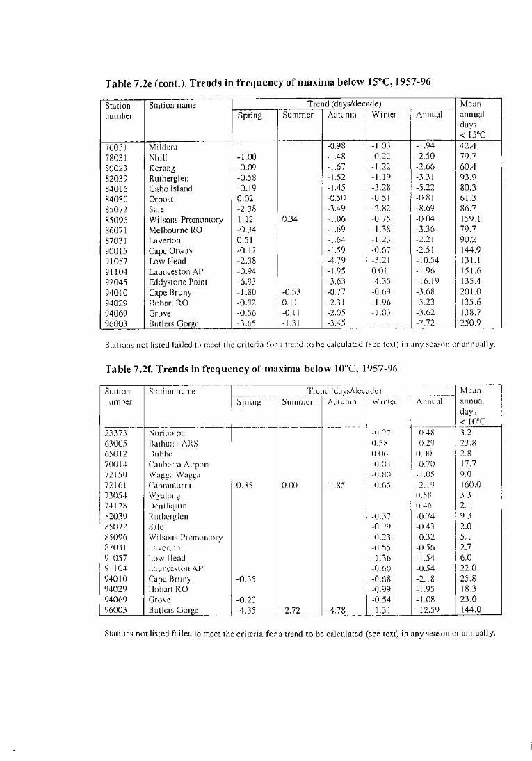
Table 7 .2e (cont.). Trends in frequency of maxima below l5°C, 1957-96
Station Station name Trend (days/decade) Mean number Spring Summer Autumn Winter Annual annual
days < 15°C
76031 Mil dura -0.98 -1.03 -1.94 42.4
78031 Nhill -1.00 -1.48 -0.22 -2.50 79.7
80023 Kerang -0.09 -1.67 -1.22 -2.66 60.4 82039 Rutherglen -0.58 -1.52 -1.19 -3.31 93.9 84016 Gabo Island -0.19 -1.45 -3.28 -5.22 80.3 84030 Orbost 0.02 -0.50 -0.51 -0.81 61.3 85072 Sale -2.38 -3.49 -2.82 -8.69 86.7 85096 Wilsons Promontory 1.12 0.34 -1.06 -0.75 -0.04 159.1 86071 Melbourne RO -0.34 -1.69 -1.38 -3.36 79.7 87031 Laverton 0.51 -1.64 -1.23 -2.21 90.2 90015 Cape Otway -0.12 -1.59 -0.67 -2.51 144.9 91057 Low Head -2.38 -4.79 -3.21 -10.54 131.1 91104 Launceston AP -0.94 -1.95 0.01 -1.96 151.6 92045 Eddystone Point -6.93 -3.63 -4.35 -16.19 135.4 94010 Cape Bruny -1.80 -0.53 -0.77 -0.69 -3.68 201.0 94029 Hobart RO -0.92 0.11 -2.31 -I. 9(> -5.23 135.6 94069 Grove -0.56 -0.11 -2.05 -1.03 -3.62 138.7 96003 Butlers Gorge -3.65 -1.31 -3.45 -7.72 250.9
Stations not listed failed to meet the criteria for a trend to he calculated (sec text) in any season or annually.
Table 7 .2f. Trends in frequency of maxi nut below 1 ooc, 1957-96
Station Station name Trend (days/decade) Mean ---·" ___ number Spring Summer Autun1n Winter Annual annual
days < 10°C
··- -·
23373 Nuriootpa -0.27 -0.48 3.2 63005 Bathurst ARS 0.)~ -0.2') 23.8 65012 Dubho 0.0(> 0.00 2.8 70014 Canberra Airport -0.04 -0.70 17.7 72150 Wagga Wagga -O.kO -1.05 9.0 72161 Cahramurra O.J5 0.00 -1.8) -0.()5 -2.19 160.0 73054 Wyalong 0.58 3.3 74128 Dcniliquin ().4() 2.1 82039 Ruthcrglcn -0.37 -0.74 9.3 85072 Sale -0.29 -0.43 2.0 85096 Wilsons Promontory -0.23 -0.32 5.1 87031 Laverton -0.55 -0.56 2.7 91057 Low Head -1.36 -1.54 6.0 91104 Launceston AP -0.60 -0.54 22.0 94010 Cape Bruny -0.35 -0.68 -2.18 25.8 94029 Hobart RO -0.99 -1.95 18.3 94069 Grove -0.20 -0.54 -1.08 23.0 96003 Butlers Gorge -4.35 -2.72 -4.78 -1.31 -12.59 144.0
Stations not listed failed to meet the criteria for a trend to be calculated (see text) in any season or annually.

Table 7.2g. Trends in frequency of minima below soc, 1957-96
Station Station name Trend (days/decade) Mean number Spring Summer Autumn Winter Annual annual
days <soc
7045 Meekatharra -0.87 -0.81 12.6 8039 Dalwallinu -1.34 -1.04 -2.66 28.1 8051 Gerald ton 0.01 -0.54 -0.57 7.4 9021 Perth Airport -0.56 -0.78 -2.45 16.1 9741 Albany -I .38 -5.41 -7.37 25.8 9789 Esperance -1.44 -2.53 6.5 10035 Cunderdin -1.70 -2.16 -3.99 46.7 10648 Wandering -2.43 -1.55 -2.90 -6.90 95.3 11052 Forrest -1.23 0.82 0.44 -0.20 63.2 12038 Kalgoorlie -1.96 -1.74 -2.82 -6.50 62.5 13017 Giles 0.19 -0.13 18.6 15548 Rabbit Flat* 0.96 0.75 29.0 15590 Alice Springs -0.80 -0.85 -0.62 -2.29 66.3 16001 Woomera -1.23 -4.39 30.4 16044 Tarcoola -1.81 0.09 -0.65 -2.33 61.2 17031 Marrec -0.75 -2.10 -3.48 46.6 17043 Oodnadatta 0.12 -1.24 -1.17 39.9 18012 Ceduna -3.06 -0.78 -3.84 -7.83 62.1 18070 Port Li nco! n -1.30 -1.48 3.6 21046 Snowtown 0.65 -0.72 -2.30 -1.61 60.6 22801 Cape Borda -0.65 -0.74 2.4 23090 Adelaide RO -0.50 -3.69 -4.08 21.1
23373 Nuriootpa -0.21 -1.23 -4.74 -6.87 86.3 26021 Mt Gambier -1.42 -0.90 -0.81 -4.26 -7.15 72.6 26026 Robe -1.26 -1.01 -2.08 12.3 30045 Richmond -1.46 -2.10 14.5 36007 Barca! dine -1.48 -2.24 16.7 3()03 1 Longreach -0.16 -0.59 28.3 37010 Camoowca1 -0.02 -0.18 9.9
38002 Birdsvillc 0.71 -0.27 25.9
38003 Boulia -1.19 -1.11 12.6
39039 Gayndah -1.91 -2.85 30.2
39083 Rockhampton -2.90 -3.23 11.2 39128 Bunuahcrg -1.29 -1.27 5.5
40004 Ambcr1ey 0.24 -1.41 -1.59 -2.66 54.3
40223 Brisbane Airport -3.73 -3.71 15.2
42023 Miles 0.57 -2.39 -2.76 -4.20 67.0
43109 St. George -1.01 -2.86 37.0
44021 Charlevillc -1.71 -2.01 -3.65 -7.85 66.9 45017 Thargomindah -1.99 -2.77 38.1
46037 Tibooburra -0.27 -0.82 37.4
46043 Wilcannia -0.20 0.84 -0.61 -0.14 51.7
48027 Co bar -0.87 -1.82 -3.05 -5.74 54.0
48239 Bourke -2.38 -3.29 45.2
52088 Walgett -0.41 -2.32 -1.88 -4.10 72.3
53048 Moree -1.26 -3.89 -3.14 -8.30 70.5
55024 Gunnedah Soil Cons -0.43 -1.30 -2.14 -3.89 50.2
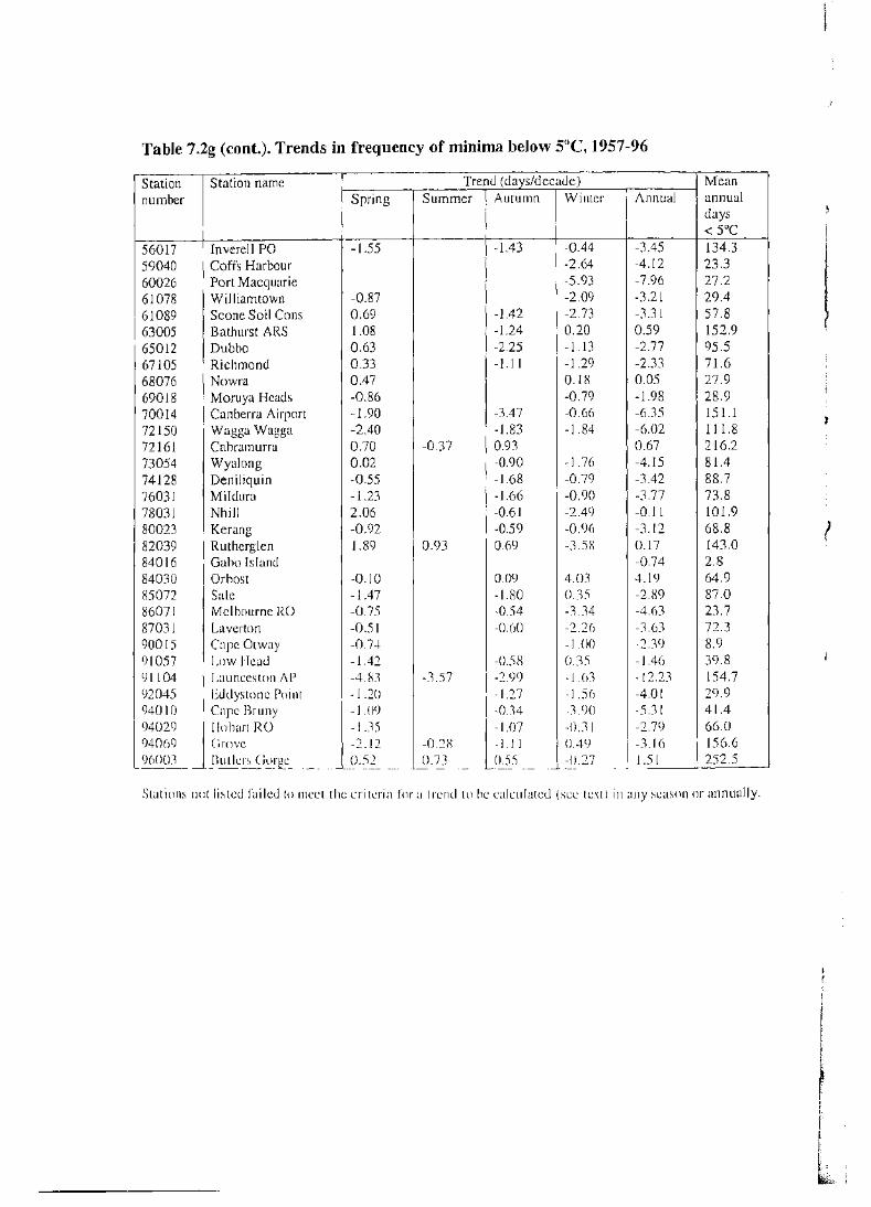
Table 7.2g (cont.). Trends in frequency of minima below soc, 1957-96
Station Station name Trend (days/decade) Mean number Spring Summer Autumn Winter Annual annual
days <soc
56017 Inverell PO -1.55 -1.43 -0.44 -3.45 134.3 59040 Coffs Harbour -2.64 -4.12 23.3 60026 Port Macquarie -5.93 -7.96 27.2 61078 Williamtown -0.87 -2.09 -3.21 29.4 61089 Scone Soil Cons 0.69 -1.42 -2.73 -3.31 57.8 63005 Bathurst ARS 1.08 -1.24 0.20 0.59 152.9 65012 Dubbo 0.63 -2.25 -1.13 -2.77 95.5 67105 Richmond 0.33 -1.11 -1.29 -2.33 71.6 68076 Nowra 0.47 0.18 0.05 27.9 69018 Moruya Heads -0.86 -0.79 -1.98 28.9 70014 Canberra Airport -1.90 -3.47 -0.66 -6.35 151.1 72150 Wagga Wagga -2.40 -1.83 -1.84 -6.02 111.8 72161 Cabramurra 0.70 -0.37 0.93 0.67 216.2 73054 Wyalong 0.02 -0.90 -I. 76 -4.15 81.4 74128 Deniliquin -0.55 -1.68 -0.79 -3.42 88.7 76031 Mildura -1.23 -1.66 -0.90 -3.77 73.8 78031 Nhill 2.06 -0.61 -2.49 -0.11 101.9 80023 Kerang -0.92 -0.59 -0.96 -3.12 68.8 82039 Rutherglen 1.89 0.93 0.69 -3.58 0.17 143.0 84016 Gaho Island -0.74 2.8 84030 Orhost -0.10 0.09 4.03 4.19 64.9 85072 Sale -1.47 -1.80 0.35 -2.89 87.0 86071 Melbourne RO -0.75 -0.54 -3.34 -4.63 23.7 87031 La vert on -0.51 -0.(l0 -2.2(l -3.63 72.3 90015 Cape Otway -0.74 -1.00 -2.39 8.9 91057 Low Head -1.42 -0.58 0.35 -1.4() 39.8 91104 Launceston AP -4.83 -3.57 -2.99 -l.(l] -12.23 154.7 92045 Eddystone Point -I .20 -1.27 -1.5() -4.01 29.9 940IO Cape Bruny -1.09 -0.34 -3. C)() -5.31 41.4 94029 IIohart RO -1.35 -1.07 -0.31 -2.79 66.0 940()9 Grove -2.12 -0.2)-; -1.1 I 0.49 -3.16 156.6 96003 Butlers Gorge 0.52 0.73 0.55 -0.27 1.51 252.5
.•.
Stations not listed failed to meet the criteria for a trend to be calculated (sec text) in any season or annually.

Table 7.2h. Trends in frequency of minima below 2°C, 1957-96
Station Station name Trend (days/decade) Mean number Spring Summer Autumn Winter Annual annual
days <2°C
8039 Dalwallinu -1.10 -1.42 3.4 10035 Cunderdin -0.91 -1.91 9.2 10648 Wandering -2.97 -0.81 -1.51 -5.17 40.7 11052 Forrest -2.09 -1.74 16.6 12038 Kalgoorlie -2.30 -3.21 19.9 15548 Rabbit Flat* -0.59 -0.53 9.4 15590 Alice Springs -1.32 -2.76 33.4 16044 Tarcoola -1.88 -2.10 21.5 17031 Marrec -2.55 -2.54 12.3 17043 Oodnadatta -0.91 -0.68 10.4 18012 Ceduna -2.13 -4.27 -7.35 21.9 21046 Snowtown -0.02 -2.12 -2.26 15.4 23373 Nuriootpa -0.57 -1.08 -5.68 -7.34 36.0 26021 Mt Gambier -1.08 -0.91 -3.38 -5.36 18.7 36031 Longreach -1.26 -1.38 8.2 39039 Gayndah -1.31 -1.54 7.6 40004 Amberley -2.11 -2.36 25.2 42023 Miles -2.10 -3.48 33.8 43109 St. George -1.21 -1.37 9.0 44021 Charleville -1.64 -2.91 28.1 45017 Thargominuah -0.64 -0.76 8.2 46037 Ti boohurra -0.34 -0.24 7.9 46043 Wilcannia 0.11 0.44 13.0 48027 Cohar -3.49 -3.76 15.5 48239 Bourke -1.88 -1.77 9.9 52088 Walgctt -0.60 -1.43 29.3 53048 Moree -0.91 -3.78 -6.39 32.0 55024 Gunncuah Soil Cons -2.22 -2.90 14.7 56017 Invcrcll PO -1.46 -1.26 -1.28 -3.97 91.6 59040 ColTs 1 I arbour -2.01 -2.32 5.8 61078 Williamtown -1.76 -1.88 5.6 61089 Scone Soi I Cons -0.66 -1.08 18.8 63005 Bathurst ARS 0.90 -1.66 -0.82 -1.39 88.9 65012 Dubho -1.33 -1.95 -2.05 -5.30 51.7 ()7105 Richmond -0.49 -0.88 31.6 70014 Canberra Airport -1.97 -2.80 -1.54 -6.40 93.7 72150 Wagga Wagga -0.45 -0.84 -2.60 -3.86 51.9 72161 Cabramurra 0.71 -0.29 -1.77 -1.07 -2.44 150.9 73054 Wyalong -0.14 -0.62 -2.75 29.3 74128 Deniliquin 0.42 0.02 0.12 29.3 76031 Mildura -0.55 -1.03 -2.77 -4.34 24.9 78031 Nhill 0.29 -0.72 -1.53 -1.85 37.8 80023 Kerang -3.49 -3.88 16.1 82039 Rutherglen 1.08 -0.18 -2.08 -0.97 75.4 84030 Orbost 1.05 1.37 16.1 85072 Sale 0.67 -0.43 2.41 2.64 27.1 86071 Melbourne RO -1.40 -1.51 3.8 87031 Laverton 0.40 -1.70 -2.48 19.8
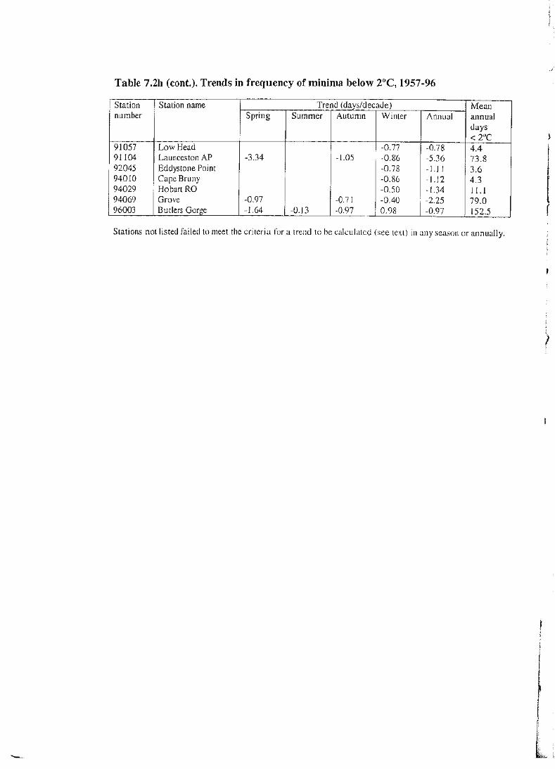
Table 7.2h (cont.). Trends in frequency of minima below 2°C, 1957-96
Station Station name Trend (days/decade) Mean number Spring Summer Autumn Winter Annual annual
days < 2°C
91057 Low Head -0.77 -0.78 4.4 91104 Launceston AP -3.34 -1.05 -0.86 -5.36 73.8 92045 Eddystone Point -0.78 -1.11 3.6 94010 Cape Bruny -0.86 -1.12 4.3 94029 Hobart RO -0.50 -1.34 11.1 94069 Grove -0.97 -0.71 -0.40 -2.25 79.0 96003 Butlers Gorge -1.64 -0.13 -0.97 0.98 -0.97 152.5
Stations not listed failed to meet the criteria for a trend to be calculated (see text) in any season or annually.

Table 7.2i. Trends in frequency of minima below 0°C, 1957-96
Station Station name Trend (days/decade) Mean number Spring Summer Autumn Winter Annual annual
days < ooc
10648 Wandering -1.10 -1.77 -3.41 14.5 12038 Kalgoorlic -0.88 -1.09 5.1 15590 Alice Springs -0.77 -0.96 14.6 16044 Tarcoola -0.96 4.3 18012 Ceduna -2.74 -3.75 6.5 21046 Snowtown -1.00 -0.91 3.0 23373 Nuriootpa -5.08 -5.54 15.4 26021 Mt Gambier -2.46 4.8 40004 Amherley -0.57 -0.63 10.3 42023 Miles -3.04 -3.19 17.1 44021 Charleville -1.89 -2.17 12.6 52088 Walgett -0.67 -0.66 10.7 53048 Moree -3.84 -4.76 13.0 55024 Gunnedah Soil Cons -1.39 -1.60 3.0 56017 Invercll PO -0.43 -1.30 -2.36 -4.06 59.7 61089 Scone Soil Cons -0.25 -0.16 4.4 63005 Bathurst ARS 0.06 -1.65 -2.02 -3.49 54.8 65012 Duhho -0.45 -2.79 -3.55 23.2 67105 Richmond -0.86 -0.94 12.7 70014 Canberra Airport -1.44 -2.77 -1.48 -5.70 63.0 72150 Wagga Wagga -0.58 -2.01 -3.19 24.4 72161 Cahramurra 0.01 -2.04 0.36 -1.96 97.4 73054 Wyalong -0.21 -0.23 8.0 74128 Deniliquin -0.50 -0.48 8.1 7()031 Mildura -1.24 -1.32 5.8 78031 Nhill -0.16 -0.99 -1.18 -2.30 13.7 80023 Kcrang -0.44 3.1 82039 Ruthcrglcn -0.14 -0.16 -2.27 -2.45 39.5 84030 Orhost 0.04 2.7 85072 Sale !.12 0.91 7.6 87031 La vert on -0.31 -0.72 4.9 91104 Launccston AP -1.36 -0.92 -1.85 -3.76 34.9 CJ4069 Grove -0.39 -0.60 -1.06 -2. I 8 37.0 CJ(>003 Butlers Gorge 0.34 -0.29 0.36 1.87 2.72 8!.7
Stations not listed faileu to meet the criteria for a trend to he calculated (sec text) in any season or annually.

Table 7.3. Percentage of stations with upward trends of percentile threshold ~even t f 1957 96 requency, -Threshold Season State
WA NT SA Qld NSW Vic Tas A us 5% minimum Spring 21 0 8 8 24 45 14 18
Summer 26 0 25 25 44 45 14 29 Autumn 26 40 17 14 8 36 14 18 Winter 1 1 20 0 4 24 23 14 12 Annual 21 0 0 8 16 36 29 16
10% minimum Spring 16 0 8 12 20 55 () 17 Summer 21 0 33 12 40 36 21 25 Autumn 21 20 17 12 4 27 () 14 Winter 21 0 0 8 16 27 14 14 Annual 21 0 0 12 20 36 14 17
9Qlfl) minimum Spring 84 100 67 88 64 73 86 78 Summer 58 80 67 79 84 64 57 72 Autumn 74 80 83 92 84 55 86 81 Winter 84 80 83 88 96 64 71 84 Annual 84 100 83 92 92 73 71 86
95% minimum Spring 84 80 58 92 60 73 86 76 Summer 58 60 58 87 68 55 57 67 Autumn 68 80 92 92 80 64 86 81 Winter 84 80 75 79 84 64 86 80 Annual 84 100 83 96 80 73 71 84
5% maximum Spring 42 40 0 71 40 18 0 38 Summer 53 40 25 29 52 82 57 47 Autumn 21 60 0 21 20 27 0 19 Winter 42 0 8 58 32 18 14 33 Annual 42 20 8 12 24 36 0 22
-·-·-·
1 oc~J maximum Spring 37 20 8 50 28 32 0 31 Summer 71 20 42 21 52 73 29 46 Autumn 21 20 0 8 8 9 0 10 Winter 32 0 8 50 24 9 29 27 Annual 2() 20 8 8 12 9 0 13
90c~, maximum Spring 74 80 58 71 52 45 71 37 Summer 42 60 58 83 56 0 29 48 Autumn 74 80 75 58 32 73 lOO 38 Winter 89 100 83 79 80 64 lOO 17 Annual 74 100 83 83 60 ()4 86 25
------·-----·-~-~----- " --------·---·-·-------<JS% maximum Spring 74 80 58 71 68 36 71 66
Summer 48 60 ()7 75 44 27 43 53 Autumn 74 80 75 54 28 73 100 ()()
Winter 84 100 92 79 80 91 100 85 Annual 74 80 83 79 60 64 86 73
--

Table 7.4. Percentage of stations with upward trends of fixed threshold event fr~qucncy, 1957-96
-- "~ .... -. ~- ,, .. ., ... _______ ,__, _________ . ___ ..........__
Thr c:sh<dd Seas<>n State r-----~---,-------~
WA NT SA Qld NSW Vic Tas A us Max > ~()h(' Spring 60 100 50 82 56 37 63
Summer 50 67 50 81 74 20 33 60 Autumn 78 60 60 83 18 12 57 Winter 80 lOO 67 78 Annual 68 100 50 96 61 10 33 66
Ma X > :~S"C. Spring 47 60 50 69 17 0 51 Summer 50 75 40 83 71 12 59 Autumn 71 75 60 56 88 100 68 Winter 100 () 50 Annual 5() 100 40 85 56 78 60
Ma -------... - r-·
0 53 X > .. l()"(' Spring 50 (J7 67 50 Summer (>() 75 67 67 83 67 67 Autumn 50 50 Winter Annual (l5 75 57 80 50 67 66
----~~~--~--~ ·-··
Ma X·::: lYC' Spring 0 0 27 30 0 15 Summer 100 100 25 50 Autumn 0 0 12 0 0 3 Winter 3] () C) 100 36 0 17 27 Annual 25 0 0 75 26 0 0 18 -
Ma X< I()"(. Spring 100 0 25 Summer 50 0 25 Autumn 0 0 0 Winter 0 40 0 0 12 Annual 0 36 0 0 14
·····-···-~-·
l\.1tr l > ~)()"(. Spring 70 100 60 78 88 78 Summer ()<) 100 70 83 91 33 77 Aut un1n 77 75 80 74 60 73 Winter J] 100 60 56 Annual 72 100 60 78 86 43 75
·-··----1 ,· •)"(. Spring 12 () 14 67 39 22 14 26
Summer () 0 100 33 33 Autumn 33 () 29 0 13 22 14 18 Wi11ter 1 s 50 0 7 10 22 29 13
/\JJnual () 50 0 0 14 20 14 9 --
\!1 33 80 0 32 II ·• ~ "( , Spring () 0 Sutntner 0 0 0 ;\utumn () 0 0 0 0 0
Winter () () 0 0 II 25 14 9
Annual () () 0 0 11 25 0 7 ~-.--~----- ..
33 0 33 25 11 < ()"(' Spring ()
Summer 0 0
Autumn 0 0 33 11
Winter 0 0 0 0 8 20 33 10
Annual 0 0 0 0 0 29 33 9

7.1.2.1. High maximum temperatures
All indices of extreme high maximum temperatures show a general increasing trend,
although these trends are smaller than those for any of the other extreme events
considered. Seventy-four percent of stations show an increase in the frequency of
temperatures above the 90th percentile, 72% an increase in the frequency of
temperatures above the 95th percentile, and 66%, 60% and 66% an increase in the
frequency of temperatures over 30°C, 35°C and 40°C respectively.
For the percentile thresholds, the most coherent area of decreasing trends is in inland
New South Wales, along with the coast of southern New South Wales and eastern
Victoria. Other areas of decreasing trends are found in north-western Queensland and
the southern coasts of Western Australia and western South Australia. Most other
stations show increases, with scattered exceptions. The strongest increasing trends
(generally more than 5 days/decade for the 90th percentile) occur on the east coast of
Queensland north of B undaberg, in parts of central Australia, and in northern
Tasmania.
Examining the seasonal breakdown, substantial areas of seasonal decreasing trends
are found in the following areas:
l8 spring: south-eastern South Australia, southern New South Wales and most or Victoria (except the west coast), along with notih-western Queensland.
l8 sun1mer: south-western Westetn Australia, parts of inland northern NSW, all
or Victoria and most of Tasmania, and much of the far north of Australia.
•• autumn: parts of south-westetn Weste111 Australia, south-eastern Queensland
and most of New South Wales (except the north coast and far south), and parts
of north-western Queensland and the Northern Ten·itory.
•• winter: north-western Queensland and the south coast of New South Wales.
The proportion of stations showing increasing trends is greatest in winter (83% for the
90th percentile), and least in summer and autumn (52% and 62% respectively).
151

The goth and 95th percentiles show generally similar trends and spatial distribution of
changes, although one interesting difference between the two occurs in summer in
south-eastern Australia: the Sydney region shows an increase in the frequency of
maxima above the 90th percentile but a decrease in the frequency of maxima above the
951h percentile, whereas the reverse is true in parts of northern Victoria.
The results for fixed thresholds follow some similar patterns to the percentile
thresholds - such as a tendency to strong increases in coastal Queensland and
decreases along the southern coasts. Differences between the two largely reflect
differences in where the fixed thresholds fit in the climate of a particular region and
season. Examples of substantial differences include:
• most stations in Victoria and southern New South Wales show a decrease in
the frequency of maxima above the fixed thresholds. This matches the
observed trends for summer, but not for the year as a whole, for the percentile
thresholds, which is an unsurprising result as maxima above 30°C (and, even
more so, 3s<> and 40°C) in this region are largely a summer phenomenon.
• most Queensland stations show an increase in the frequency of autumn
maxima above 30°C, whereas there is little trend for the percentile thresholds.
This reflects the fact that 30°C is not a particularly extreme event in most of
Queensland during that season. This trend is not observable when a 35°C
threshold is used.
7 .1.2.2. High minimum temperatures
All indices of extreme high minima show increasing trends. Eighty-three percent of
stations show an increase in the frequency of minima above the 90th percentile, and
86% show an increase in the frequency of minima above the 95th percentile. Seventy
six percent of stations for which the index was defined show an increase in the
frequency of minima above 20°C.
The strongest increasing trends appear in Queensland, particularly the north-eastern
half, and the Northern Territory, with many stations in this area showing trends for the
152

90th percentile in excess of 5 days/decade. The only coherent areas of stations with a
decreasing annual trend for any of the thresholds are in south-eastern New South
Wales and eastern Victoria, and in northern South Australia and western Queensland.
A few scattered and widely separated stations in other regions also show decreasing
trends.
The proportion of stations with increasing trends is greatest in winter (84% for the
90th percentile), and least in summer (72%). Notable regional areas of decreasing
trends are:
~~ spring: parts of inland New South Wales, eastern Victoria, northern South
Australia and south-western Queensland.
~~ summer: south-western Western Australia, and scattered stations tn central
Australia and Victoria.
11 autumn: eastern Victoria.
11 winter: parts of northern Western Australia.
Stations with a decreasing trend in the frequency of minima above the fixed threshold
of 20°C are scattered in all seasons, with the most coherent region of such trends in
any season being in the south-western half of Queensland in auturnn. The strongest
increasing trends, as for the percentile thresholds, are in the Northern Territory and on
the coasts or Queensland and northern New South Wales.
7 .1.2.3. Low maxin1un1 ten1peratures
All indices of extreme low maximum temperatures show a decreasing trend at the vast
rnajority of stations. Seventy-eight percent of stations have recorded a decrease in the
frequency of maxima below the lOth percentile, and 87% a decrease in the frequency
of maxima below the 5th percentile. For the fixed thresholds, the figures are 83% for
rnaxima below l5°C and 86% for maxima below l0°C, although it should be noted
that the latter index is only defined at 18 of the 103 stations, and at only four stations
is it defined in any season other than winter.
153
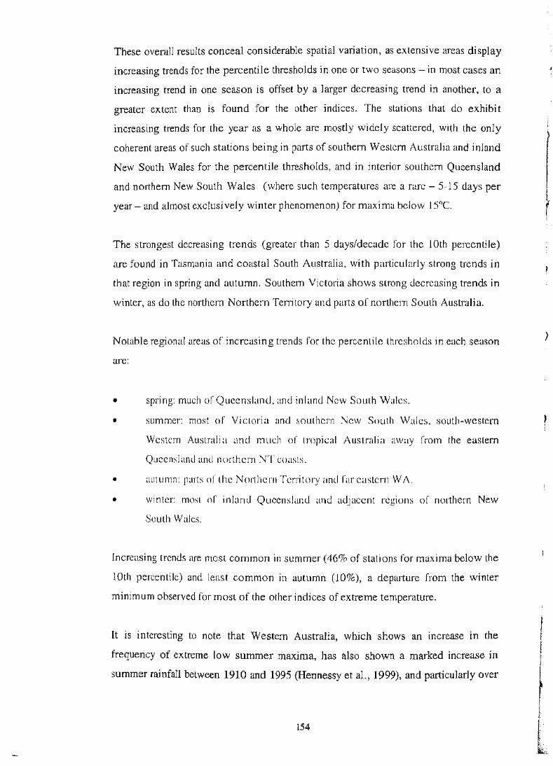
These overall results conceal considerable spatial variation, as extensive areas display
increasing trends for the percentile thresholds in one or two seasons -in most cases an
increasing trend in one season is offset by a larger decreasing trend in another, to a
greater extent than is found for the other indices. The stations that do exhibit
increasing trends for the year as a whole are mostly widely scattered, with the only
coherent areas of such stations being in parts of southern Western Australia and inland
New South Wales for the percentile thresholds, and in interior southern Queensland
and northern New South Wales (where such temperatures are a rare- 5-15 days per
year- and almost exclusively winter phenomenon) for maxima below 15°C.
The strongest decreasing trends (greater than 5 days/decade for the 1Oth percentile)
are found in Tasmania and coastal South Australia, with particularly strong trends in
that region in spring and autumn. Southern Victoria shows strong decreasing trends in
winter, as do the northern Northern Territory and parts of northern South Australia.
Notable regional areas of increasing trends for the percentile thresholds in each season
are:
• spring: much of Queensland, and inland New South Wales.
• summer: most of Victoria and southern New South Wales, south-western
Western Australia and 1nuch of tropical Australia away from the eastern
Queensland and northern NT coasts.
• autumn: parts of the Northern Territory and far eastern W A.
• winter: most of inland Queensland and adjacent regions of northern New
South Wales.
Increasing trends are most common in summer ( 46% of stations for maxima below the
lOth percentile) and least common in autumn (10%), a depatiure from the winter
minimum observed for most of the other indices of extreme temperature.
It is interesting to note that Western Australia, which shows an increase in the
frequency of extreme low summer maxima, has also shown a marked increase in
summer rainfall between 1910 and 1995 (Hennessy et al., 1999), and particularly over
154
)

the 1957-1996 period, with the trend accelerating in the later years of that period (see
Fig. 7 .3). In most of Australia away from the southern coasts extreme low maxima in
summer mostly occur as a result of persistent cloud cover and/or rain (rather than
through the presence of an air mass of southern origins), so this combination of results
is not especially surprising.
The marked decrease in the frequency of extreme low maxima in the winter half of
the year over those regions of south-eastern Australia that are particularly exposed to
westerly and south-westerly flow may point to synoptic changes. An analysis of
possible synoptic changes is beyond the scope of this thesis, but the possible
implications of changes in the frequency distribution of maximum temperature are
discussed in section 7.2.
7 .1.2.4. Low minimum ten1peratures
The declining frequency of low mini mum temperatures is the strongest trend for any
of the four types of extre1ncs considered in this study. This is particularly true of the
fixed thresholds; more than 90~) of stations show a decreasing trend in the frequency
of minima below 5°C, 2°C and 0°C. The trend is not so striking for the percentile
thresholds, but 84(Yc) of stations still show a decreasing trend in the frequency of
rninima below the 5th percentile, and 83% for the lOth percentile.
rllhose stations which do show increasing trends for any of the indices arc mostly
widely scattered. The one region with a number of stations showing increasing trends,
particularly for the percentile thresholds, is eastern Victoria and south-eastern New
South Wales. Particularly strong declines have occuned in much of Queensland and
the Northern Territory, the south-west of Western Australia and southern South
Australia, with 1nany stations in those regions showing trends in excess of 5
days/decade for the lOth percentile, and some exceeding 10.
All seasons and thresholds show a strong majority of stations with decreasing trends.
As for the other indices, the proportion is smallest in summer (75% for miniina below
the lOth percentile) and greatest in winter (86%), but the seasonal differences are
weaker than for the other indices.
155
Regions where a number of stations with increasing trends can be found for the
percentile thresholds are:
• spring: much of northern Victoria and the tablelands of New South Wales.
• summer: the southern two-thirds of New South Wales, eastern Victoria and
weste111 Queensland.
• autumn: eastern Western Australia.
• winter: eastern Victoria and the far south-east of New South Wales .
As the previously noted results would suggest, stations showing an increasing trend
for any of the fixed thresholds over the year as a whole are very rare. A notable
seasonal exception, however, is that many Victorian and elevated New South Wales
stations show an increase in the frequency of low minimum temperatures (particularly
when 2°C is used as the threshold) in spring. As this is a region where late spring
frosts are already an agricultural hazard (and either 2°C, or, historically, 36°F (2.2°C),
has been routinely used as a threshold to determine the occurrence of frost in
Australia (e.g. Foley, 1945)), this is a result of some potential significance.
7 .1.3. Results over extended periods starting before 1957
The analysis of trends in the frequency of extreme temperature events prior to 1957 is
made difficult, as discussed in Chapter 2, by the lack of digitised daily temperature
data prior to that elate. Of the 103 stations in the data set, only nine have 60 years or
more of data, and three of these (Adelaide, Melbourne and Sydney) are city-centre
sites where the existence of urban heat islands limit the use of the data for the analysis
of climate change. There is a project cunently in progress to digitise more historical
daily data, which will enable such trends to be calculated over a longer period at many
more stations, and over a much greater proportion of the Australian continent.
The remaining six stations, all in New South Wales, have data commencing in 1921 -
the Moree data commences earlier, but the variety of instrument exposures in
existence in New South Wales prior to 1908 (Torok, 1996; also discussed in the
156
, r f

diaries of H.C.Russell, held in the National Meteorological Library) render that data
difficult to use without reference to comparison data (which does not exist in a
digitised form) fr01n neighbouring stations. The 1921-56 data should still be treated
with some caution because of a similar lack of comparison data for use in making
adjustments for inhomogeneities.
Tables 7.5 and 7.6 show the observed trends for the percentile and fixed thresholds at
the six stations for each season over the 1921-96 period. The spatial distribution of
positive and negative trends is quite similar to those for the shorter 1957-96 period,
with strong warming trends for most thresholds at the northern coastal sites (Yamba
and Port Macquarie) and Tiboobun·a in the north-west, and more mixed results at
l\.1oruya, on the south coast, and Bathurst and Moree in central regions of the state.
Also, similarly to the situation for the 1957-96 period, there is little statewide trend in
the frequency of high maxi1num temperatures (and the decreasing trend in autumn
which is so marked in 1957-96 is also visible for 1921-96), but a discernable trend for
the other types of extreme events.
A comparison of the 1921-96 trends with those over the 1957-96 period is
illuminating. or the 48 percentile trends examined (8 indices at 6 stations), 35 show a
'warmer' trend over the 1957-96 period than over the full 1921-96 period, indicating
an acceleration of a warming trend in temperature extremes over New South Wales
over the last 40 years. This is consistent with the Australian annual mean ten1perature
(http://www .bom.gov.au/cl i mate/change/archi ve/mediaOO.shttnl), which showed 1 i ttlc
trend over the 1921-56 period before beginning a marked increase in the late 1950's.
7 .2. Observed changes in parameters of frequency distributions of ten1perature
Changes in the parameters of the frequency distribution of daily maximUin and
rninimum temperature were examined. This was canied out by breaking the time
period of common record of most stations, 1957-1996, into two equal parts, 1957-
1976 and 1977-1996.
For each station and month, and for maximum and minimum temperature separately,
the parameters of the frequency distribution were calculated for each of these two
157

periods, treating each as a separate distribution and using the compound Gaussian
distribution model and decomposition procedure described in Chapter 6. For reasons
of computational simplicity, only those stations/months where two component
distributions had been found for the full period of record were used. This excluded 9%
of station-months for maximum temperature and 12% for minima.
Two component distributions were used for each 20-year period. The two-distribution
model was used, even though, in some cases, this model may have failed a goodness
of-fit test for an individual 20-year period.
Rabbit Flat and Learmonth were excluded from this part of the analysis, due to a lack
of data in the 1957-1976 period.
The parameters of the component distributions for each 20-year period are given in
Appendix D (Tables D.la, D.lb).
7.2.1. The relationship between observed changes in threshold event frequency
and changes predicted by the compound Gaussian distribution
)
In order to verify the effectiveness of the compound Gaussian dist1ibution in ~
modelling changes in the frequency or threshold events, the changes in the frequency
of four threshold events (maxima and minima with a normalised value, z (as defined
in Chapter 6) above +3.0 or below -3.0) in each of the four seasons were examined.
The threshold of +1- 3.0 was chosen for consistency with the checks cmTied out on the
overall effectiveness of the compound Gaussian distribution in modelling the
frequency of extreme temperature events in Chapter 6.
The expected frequencies of these events from the modelled frequency distributions
were calculated for the periods 1957-76 and 1977-96. The expected percentage
change between the two periods was then calculated. This expected percentage
change was compared with the actual percentage change from observed data between
the two periods. Only stations which recorded at least one such threshold event in
both of the periods were used in the analysis.
158
~----------------

Station Station name Threshold Trend (days/decade) number Spring Summer Autumn Winter Annual
46037 Tibooburra 5% minimum -0.24 -0.99 -0.72 0.13 -1.64 1 QC~, minimum -0.34 -1.47 -1.10 -0.19 -2.85 90(fc, minimum 0.47 1.33 0.94 0.94 3.21 9Y;f, minimum 0.23 0.64 0.48 0.48 1.74 5% maximum 0.04 0.01 -0.45 -0.12 -0.56 10% maximum -0.11 -0.07 -0.46 -0.30 -0.97 90% maximum -0.03 0.32 -0.12 0.00 0.29 95% maximum 0.00 0.24 0.07 0.41 0.79
53048 Moree 5% minimum -0.63 -0.76 -0.68 -0.78 -2.69 10% minimum -1.12 -1.36 -1.10 -1.22 -4.65 90% minimum 0.12 0.41 1.36 0.57 2.35 95% minimum -0.10 0.14 l.O 1 0.52 1.52 5% maximum 0.39 0.20 0.24 0.34 1.16 10% maximum 0.78 0.44 0.32 0.63 2.16 90% maximum -1.18 -1.47 -0.57 -0.23 -3.41 95% maximum -0.57 -0.87 -0.45 -0.21 -2.09 -
58012 Yamba 5% minimum -0.45 -0.61 -0.58 -0.81 -2.42 10% minimum -0.(J8 -0.95 -1.23 -1.23 -4.06 90% minimum 0.9() 0.75 0.62 0.24 2.58 95% minimum 0.62 0.41 0.43 0.12 1.56 5% maximum -0.47 -0.54 -1.07 -0.86 -2.99 10% maximum -0.74 -1.02 -1.48 -1.58 -4.84 90% maximum 0.64 -0.43 0.18 0.55 2.58 95% maximum 0.18 -0.33 0.16 0.32 1.56
60026 Pmt M acq uaric 5(J1) minimum -0.90 -1.14 -1.10 -1.22 -4.31 10% minimum -1.42 -2.04 -2.09 -2.2(> -7.81 90% minimum -0.12 1.45 0.76 0.63 2.75 95% minimum -0.04 0.93 0.24 0.24 1.34 5% maximum -0.78 -0.42 -0.54 -0.44 -2.10 l(Jfft, maximum -1.13 -1.01 -0.72 -1.0() -3.86 CJ()% maxi mum -0.24 1.20 0.94 0.40 2.35 95% maximum 0.22 0.69 0.34 0.30 1.57
f------- !----- " ·~-·--
(J]005 Bathurst 1\RS YJ1) minimum 0.24 0.15 0.18 -0.40 0.18
10% minimum 0.14 0.17 0.39 -O.CJO 0.14
90% minimum 0.21 -0.14 0.29 0.08 0.46 ()j(ft, minimum 0.()7 -0.22 0.10 0.00 -0.04
5% maximum 0.47 0.()3 -0.42 0.08 0.16
I 0% maxi mum 0.88 0.25 -0.53 -0.12 0.48 tJW:f, maximum -1.21 -0.58 -0.(J2 0.31 -2.10 95% maximum -0.(>7 -0.39 -0.59 0.28 -1.34
---···------·
(><J() l X Moruya l leads 5% 1ninimum 0.29 0.59 0.24 0.87 1.95
1 0% minimum 0.45 0.77 0.57 1.57 3.32
00% minimum -0.85 -0.98 -0.52 -0.30 -2.66 9Y~' minimum -0.50 -0.46 -0.2(> 0.07 -1.18
5% maximum -0.09 -0.17 -0.66 -0.57 -1.51
l 0% maximum -0.48 -0.59 -1.17 -1.38 -3.61
90% maximum -0.09 -0.48 -0.05 0.22 -0.36
95% maximum -0.25 -0.08 -0.02 0.22 -0.11
Table 7.5. Trends in frequency of percentile threshold events, 1921-1996
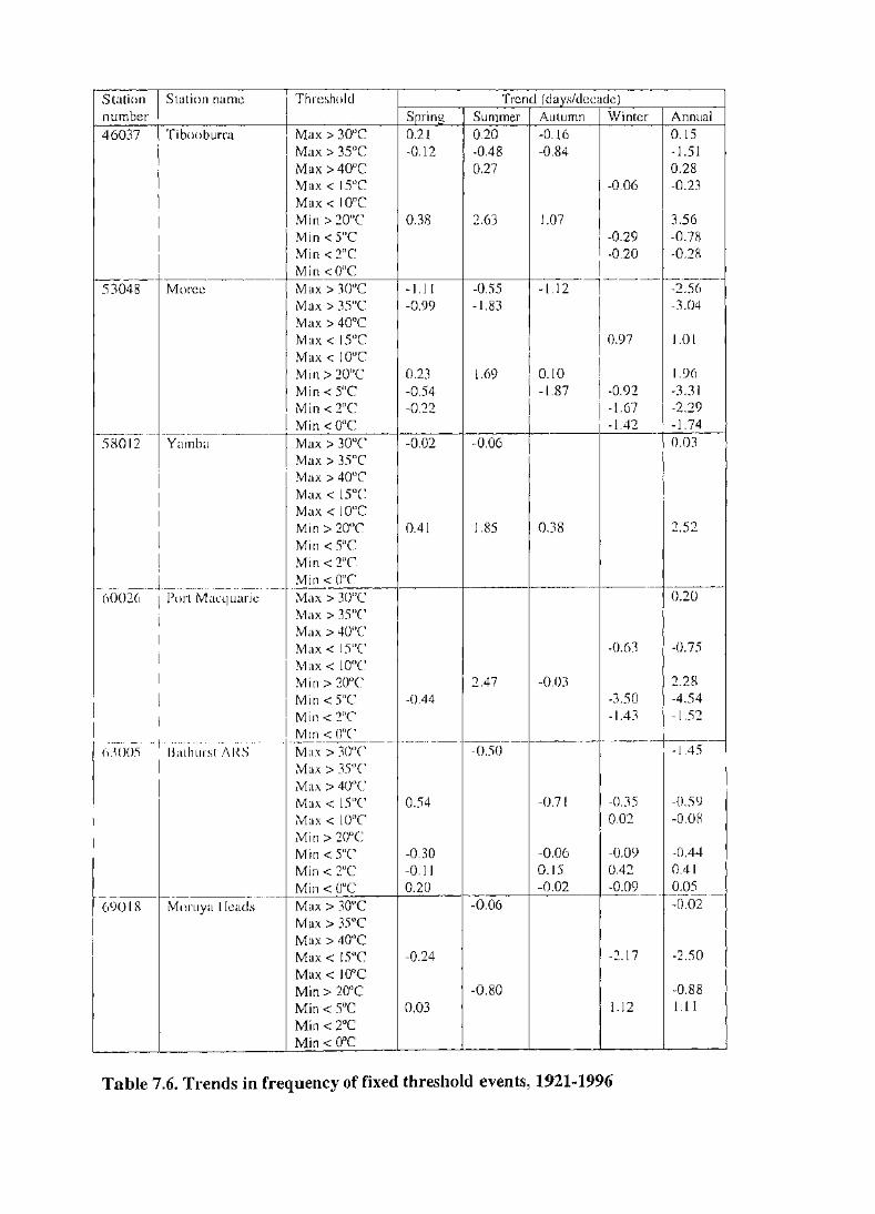
Station Station name Threshold Trend (days/decade) number Spring Summer Autumn Winter Annual 46037 Tibooburra Max> 30°C 0.21 0.20 -0.16 0.15
Max> 3SOC -0.12 -0.48 -0.84 -1.51 Max >40°C 0.27 0.28 Max< 15°C -0.06 -0.23 Max< 10°C Min> 20°C 0.38 2.63 1.07 3.56 Min< soc -0.29 -0.78 Min< 2°C -0.20 -0.28 Min <0°C
53048 Moree Max> 30°C -1.1 1 -O.S5 -1.12 -2.56 Max> 35°C -0.99 -1.83 -3.04 Max >40°C Max< 15°C 0.97 1.01 Max< l0°C Min> 20°C 0.23 1.69 0.10 1.96 Min <S°C -0.54 -1.87 -0.92 -3.31 Min <2°C -0.22 -1.67 -2.29 Min< 0°C -1.42 -1.74
58012 Yamba Max> 30°C -0.02 -0.06 0.03 Max> 35°C Max> 40°C Max< 15°C Max< JOoC Min> 20°C 0.41 1.85 0.38 2.52 Min< 5°C Min <2°C Min<(TC --···----
(>0026 Port Macquaric Max> 30°C 0.20 Max> 35"C Max> 40°C Max< 15°C -0.63 -0.75 Max< 10"C Min> 20°C 2.47 -0.03 2.28 Min<5°C -0.44 -3.50 -4.54 Min< 2oC -1.43 -1.52 Min< one
f--------- -(>.1005 Bathurst J\RS Max> 30"C -0.50 -1.45
Max> 35"C Max> 40°C Max< I5°C 0.54 -0.71 -0.35 -0.5<)
Max< I0°C 0.02 -0.08 Min> 20°C Min<S°C -0.30 -0.06 -0.09 -0.44 Min<2°C -0.11 0.15 0.42 0.41 Min< 0°C 0.20 -0.02 -0.09 0.05
69018 Moruya Heads Max> 30°C -0.06 -0.02
Max> 3S°C Max> 40°C Max< lS°C -0.24 -2.17 -2.50
Max< l0°C Min> 20°C -0.80 -0.88 Min< SOC 0.03 1.12 1.11 Min< 2°C Min< ooc
Table 7.6. Trends in frequency of fixed threshold events, 1921M1996

The results of this comparison are summarised in Table 7.7, with the full list of
comparisons in Appendix D, tables D.2a-d. Whilst the simulation using the compound
normal distribution clearly lacks precision in estimating the observed changes (the
actual change is between 0.8 and 1.2 times the simulated change in between 26% and
37% of cases, depending on the element), a reasonable simulation (actual change
between 0.5 and 1.5 times the simulated change) is achieved in between 61% and
74% of cases.
These results should be viewed with the perspective that a z value above +3.0 or
below -3.0 is a rare event, and that in many cases the observed frequency in a 20-year
period of 0.05 or 0.06o/rJ represents a single event in a 20-year period. As a result, one
event in the observed record can have a major effect on the accuracy of the simulation
for the most extreme events.
In those cases where jzj > 3.0 represents an event which occurs somewhat more
frequently at the particular station (frequency > 0.5o/CJ over the 1957-96 period), the
simulation is substantially better than it is for the set of stations as a whole, with a
single exception (which involved a very small sample). The simulated change was
between 0.5 and 1.5 times the actual change for at least 83c~} of such cases for every
clement. This suggests that the performance of the compound Gaussian distribution in
simulating the occurrence of threshold events improves as the event becomes less
extreme.
'T'hc results displayed in Table 7.7 also suggest that there is no inherent tendency for
the simulation using the compound Gaussian distribution to either over-estimate or
under-cstitnate the actual change in the frequency of threshold events.
7 .2.2. Observed changes in the frequency distribution of maxin1um and
Jtninimum ten1peratures.
Changes in the paran1eters of the component distdbutions between the 1957-76 and
1977-96 periods were examined for each station/month in which two component
distributions had been sufficient to model the distribution for the full period of record.
159

A proportion of the distributions underwent radical change between the two periods.
A distribution was considered to have undergone radical change if at least one of the
two component distributions fulfilled at least two of the following three (arbitrary)
criteria:
(a) a change exceeding 0.2 in the weight, w 1
(b) a change exceeding 0.5 in the component mean, J-ln
(c) a change exceeding 0.5 in the component standard deviation, Of1
((b) and (c) being expressed in terms of z-scores).
Station/months that fulfilled these criteria were not considered further in the analysis.
This resulted in the exclusion of between 13o/o and 23o/o of station/months (depending
on season and element).
A summary of the results from the remaining station/months is given in Tables 7.8a
and 7. 8b. In each case, distributions 1 and 2 are chosen such that ,u 1 < p2.
A majority of Australian stations show an increase in the means of both the warmer
and cooler component distributions in all seasons, and for both maximum and ~
minimum temperature. For maxi mum temperature, this trend is almost equally
observable in all seasons ror the wanner and cooler components, and is strongest in
spring and weakest in winter. For n1inimum temperature, whilst results for the year as
a whole arc similar for the two components, the warmer component shows a
particularly strong increase in autumn, whilst the cooler component shows a strong
increase in winter.
A majority of Australian stations show a decrease in the weighting of the cooler
component in all seasons and for both maximum and minimum temperature. The
decreases are more widespread for minimum temperatures than for maxima, and are
particularly pronounced for minima in winter and spring.
160

Table 7.7. Similarity between changes in frequency of extreme events Clzl > 3) observed between 1957-76 and 1977-96, and changes modelled by cornpound normal distribution
Event Element High maxima High minima Low maxima Low minima
Percentage All cases 37 26 37 32 or cases Cases with 58 67 49 25 within 201Jfl frequency> 0.5% Percentage All cases 70 61 74 68 of cases Cases with 9() 100 88 83 within 501/f, frequency> O.YYr~ Percentage or cases where actual 45 58 56 51 change> mo<.lcllcd change Total All cases 187 142 177 104 number or Cases with 78 9 51 12 cases f'retlll~ > o.srfr,

Table 7.8a. Summary of changes in parameters of frequency distributions between 1957-76 and 1977-96, maximum temperature
Season Region Percentage or cases with increase in WJ ~lJ O"J ~tl 0"2
Spring (Sep-Nov) Western Australia 56 75 50 56 50 Northern Territory 36 91 64 64 55 South Australia 60 86 41 93 66 Queensland 38 59 54 62 46 New South Wales 37 72 56 72 70 Victoria 45 71 39 75 71 Tasmania 50 94 25 81 75 Australia (total) 45 74 48 70 60
Summer (Dec-Feb) Western Australia 61 54 65 51 54 Northern Terri tory 60 80 20 70 30 South Australia 53 59 45 41 72 Queens lam] 31 72 48 76 48 New South Wales 44 60 58 70 45 Vi<.:toria 32 28 36 48 68 Tasrnania 45 58 58 47 53 Australia (total) 44 59 50 60 54
Autumn (Mar-May) Western Australia 39 68 49 49 49 Northern Territory 50 90 90 80 30 South Australia 4(> 54 46 50 63 Queensland 32 54 65 75 39 New South Wales 43 59 57 52 48 Victoria 46 54 57 57 50 Tasmania 29 93 50 93 54 Australia (total) 40 62 58 62 47
Winter (.Jun-Aug) Western Australia 64 56 52 58 47 Northern Territory 54 100 64 73 64 South Australia 38 56 36 44 56 Queensland 51 57 64 55 50 New South Wales 48 48 39 53 50 Victoria 50 77 59 55 55 Tas111ania 17 67 39 6! 67 Australia (total) 48 59 50 55 53

-·
Table 7.8b. Sun1mary of changes in parameters of frequency distributions between 1957-76 and 1977-96, minimum temperature
Season Region Percentage of cases with increase in w, Jll cr, Jll a,
Spring (Scp-Nov) Western Australia 23 66 56 78 59 Northern Territory 30 60 20 80 40 South Australia 35 65 50 54 62 Queensland 45 65 41 63 63 New South Wales 33 53 29 40 57 Victoria 42 53 53 42 74 Tasmania 61 77 58 69 54 Australia (total) 36 61 44 57 60
Summer (Dec-Feb) Western Australia 44 67 37 52 52 Northern Territory 25 75 so 50 50 South Australia 40 65 35 65 25 Queens! ami 37 59 61 75 57 New South Wales 36 52 48 65 46 Victoria so 60 58 44 48 Tasmania 50 21 43 43 36 Australia (total) 41 56 49 61 47
Autumn (Mar-May J Western Australia 35 63 45 84 55 Northern Territory 43 86 43 86 57 South Australia 43 65 35 65 57 Queensland 53 64 59 82 47 New South Wales 36 57 46 84 22 Victoria 48 48 44 48 36 Tasmania 55 63 26 74 47 Australia (total) 44 61 45 77 41
Winter (Jun-Aug) Western Australia 44 52 44 68 60 Northern Territory 14 43 43 14 86 South Australia 31 67 50 44 63 Queensland 34 60 36 47 50 New South Wales 28 (>0 44 54 51 Victoria 77 73 55 59 50 Tasnwnia 50 75 42 42 58 Australia (total) 38 61 44 51 55
-···---~ ~~-·- ··--~--~·- -·, --------- -~-~"~

The results for standard deviations of the components are much more mixed than for
means or weightings, although there is a very slight tendency towards increased
variability of maximum temperatures and decreased variability of minima. One
consistent result is that a majority of stations show a decrease in the standard
deviation of the cooler component in all four seasons.
The results observed for the distribution means suggest that the observed warming in
Australia over the 1957-96 period is distributed across all air masses, and cannot be
explained by synoptic changes alone. The changes in distribution weighting are not so
easy to interpret without knowledge of the exact air mass characteristics associated
with each component distribution (and, as has been discussed in section 6.5, it is
likely that, with only two component distributions in use, each one is an
amalgamation of several air mass types). For example, the marked decrease in the
weighting of the cooler component for winter and spring minimum temperature could
suggest an increase in cloud cover. Plummer and Power (pers.comm.) found evidence
of such an increase over the 1957-95 period over most of Australia in these seasons
(except for south-western Australia in winter), whilst Jones (1991) and Jones and
flenderson-Scllers (1992) also found an increase in cloud cover over Australia since
1910, whilst not separating results into seasonal or regional trends. One might,
however, also expect that this increase in cloud cover would be associated with an
increase in the weighting of the cooler cmnponent for maxima in these seasons. There
is no evidence or that on a national basis, although there is on a regional scale (e.g.
South Australia and Western Australia in spring, and Queensland and the Northern
Territory in winter).
The results shown are also consistent with the observation that trends in threshold
event frequency are stronger for low minima than for other types of events, as all
three parameters of the cooler component are changing in a way that has the effect of
decreasing the frequency of low minima (decreasing weight, increasing mean and
decreasing standard deviation), whereas the role of changes in component variability
is more ambiguous for the other three threshold event types. The results are, however,
less useful in explaining the relatively weak trends observed in the frequency of high
maxima.
161
Whilst it has been demonstrated in section 6.5.3 that the sensitivity of threshold event
frequency to changes in the standard deviation of the components increases (relative
to sensitivity to changes in component means or weights) as the event becomes more
extreme, the lack of evidence of consistent changes in component standard deviations
limits the applicability of that theoretical result to the observed conditions.
The relationship of changes in the distribution parameters to regional and seasonal
anomalies in threshold event trends was also examined. It was shown in section 7.1
that most threshold event indices showed their strongest warming in winter and
weakest in summer. The changes in summer distribution parameters on a national
scale, for both maxima and minima, support the notion of it being a season of
relatively weak change (the increases in component means and of the weighting of the
warmer component do not rank first amongst the seasons for any of the six
parameters). However, the changes in distribution parameters also suggest that winter
maxima should show changes as weak as those for summer, which does not match the
observed trend in threshold event frequency. This is not so pronounced for minima,
but the distribution parameters still suggest that spring and autumn, not winter, should
be the seasons with the strongest trends.
The distribution model is more accurate in handling some of the regional anmnalies
observed. A particularly interesting result is that the marked reduction in the
rrequency of low maxima observed in Tasmania, Victoria and parts of South Australia
in the cooler months appears to be associated more strongly with an increase in the
mean of the cooler component than with a decrease in its weighting. This would
suggest that the observed trend is driven by an increase in the temperature of air
masses of southerly or south-westerly origin, rather than a decrease in the frequency
of such events. It is plausible that this might be associated with an increase in winter
sea surface temperatures in the Southern Ocean, although there are insufficient pre-
1980 data available from higher latitudes in the Southe1n Ocean to allow the objective
testing of such a theory (Slutz et al., 1985).
The anomalously strong warming of minimum temperatures (and consequent marked
decrease in the frequency of low minima) observed in Queensland also appears to be
more strongly associated with changes in component means than with their weights,
162
I p

with the proportion of stations showing an increase of the mean of each of the two
components exceeding the national average in all seasons except winter. Changes in
component means are also associated with the observed cooling trends in threshold
event frequencies for summer maxima in Victoria, whilst a cooling trend in the mean
of the warmer component for spring minima in New South Wales matches an
observed decreasing trend in the frequency of high maxima.
On the other hand, Western Australia and the Northern Te1Titory show an increase in
the weight of the cooler component of summer maximum temperatures. Whilst the
component means arc still warming (weakly in Western Australia, more strongly -
albeit fr01n a small sample- in the Northern Territory), this result is consistent with
the observed increase in the frequency of low summer maxima in much of this region,
and further reinforces the possibility, first noted in section 7.1, that that change may
be driven by the increased SLllnmer rainfall in the region.
Some of the regional anomalies in observed threshold event trends arc not replicated
well by the distribution tnodel, or only match the model partially. Examples of the
latter are the observed trends in spring towards an increased frequency of low maxima
in Queensland and low n1inima in Victoria. In each case, whilst the changes in the
component n1cans suggest weaker warming than in other states (particularly in
Queensland, where the figure of 59(M-> of stations with a warming in the mean of the
cooler component for maxirna is 12~; below that for any other state), they do not
support cooling. Similarly, the results from the distribution model suggest little
change in the frequency of high autumn maxima and low summer minima in New
South Wales, whereas the observed trends point to cooling in both cases.
7 .3. Sun1n1ary
The results obtained for individual stations show that, at most stations and in most
seasons, the frequency of warm extremes (maxima and minima) has increased over
the period 1957-1996, and the frequency of cool extremes has decreased. The trends
have, in general, been stronger for cool extremes than for warm extremes, and
stronger for minima than for maxima, suggesting that a decrease in the diurnal
temperature range and a decrease in interdiutnal temperature vatiability may be
163

superimposed upon a general warming trend. The compilation of the station results
into national and regional averages will be undertaken in Chapter 8.
The general picture that emerges from an analysis of changes in the frequency
distribution is one of changes in threshold event frequencies being driven primarily by
changes in the mean temperature of air masses. Changes in component weightings,
which could suggest synoptic changes, appear to play a more limited role, with the
exception of much of tropical Australia in summer where changes in component
weights may be associated with rainfall and cloud cover changes.
164
Chapter 8
Regional Trends in Spatially Analysed Temperature Data
8.1. Introduction to the spatial analysis of temperature data
In chapters 6 and 7 the frequency of extreme temperature events at individual stations
was discussed. In order to gain a broader perspective, it is useful to analyse the frequency
of extre1ne events on a national and regional basis. This allows us to obtain a broader
picture of trends over large areas, and smnmarise the results of a study such as this in a
single result or a small number of results. It also minimises the impact of trends that may
arise from the use of individual stations whose frequency of extreme events differs from
that of their broader regions. For example, at exposed coastal stations, a reduction in the
frequency of strong offshore winds, and hence a decline in the weight of the warmer
component of the frequency distribution (as discussed in Chapters 6 and 7) is likely to
lead to a reduction in the frequency of extreme high temperatures, even if the inland
climate bccmnes hotter. The use of spatial averages furthern1ore lessens the influence of
stations (especially the n1ore isolated ones) where inhomogeneities in the record may
have been undetected or inadequately corrected for because of a lack of suitable
comparison data. When presenting the results to a non-technical audience (such as policy
rnakcrs) it is also far easier for them to understand a statement along the lines of 'The
number of days over 35°C in Australia has increased by x%' than 'Positive trends in the
frequency of maximun1 temperatures above the 95 percentile significant at the So/rJ level
were observed at y out of z stations in Australia', even if the latter is more meaningful in
a scientific sense.
The first question we n1ust confront in the spatial analysis of extreme event frequency is
whether the station network being used covers Australia sufficiently well for us to be able
to say that there is at least one station that adequately represents any given part of the
country. This issue will be discussed in section 8.2. We must also consider the 1nethods
165

used in the spatial interpolation of extreme event frequency between stations, and which
is the most appropriate for use in the context we are examining.
8.2. The spatial coherence of Australian temperature data
8.2.1. Methods for consideration of spatial coherence
As a prelude to considering spatial averages of the frequency of extreme temperature
events in Australia, h is important to consider the spatial coherence of temperature over
the country. This is examined on both the monthly and daily timescale.
The method used involves the use of the conelation between temperatures at pairs of
sites. These correlatlons are examined in two separate ways:
• Examine the pattern of correlations between a particular station and all other
stations in the data set.
• Examine the characteristic distance from a station at which the con·clation falls to
a certain level, and any tendency to strong or weak correlations in a particular
direction from a station.
The correlations arc developed usmg the set of 103 stations defined in Chapter 2. The
hasic data used arc the set or standardised departures from normal (z-scorcs) developed in
Chapter 6. For each pair of stations from arnongst the I 03, the correlation of the z-scores
between the two is determined, for n1axi1nurn and minimum temperature separately for
each of the 12 months of the year. As u separate exercise, the correlation of the monthly
means of the z-scores is also found.
For the daily conelations, all days in the record for which data are available for both
stations were used in the calculation. For the monthly conelations, all months for which a
mean is defined at both stations were used. (The requirement for a mean to be defined
was that at least 20 days (not necessarily the same 20) of observations were available.
166

The smallest number of years of record for any station pair is 18 (Learmonth and Butlers
Gorge) and the largest is 138 (Melbourne and Sydney).
For each month, for maximum and minimum temperature, this results in a set of cross
correlation coefficients for each pair of the 103 stations.
8.2.2. Patterns of correlations of daily temperature between stations
An exhaustive exan1ination of the conelation patterns for each of the 103 stations in all
seasons would clearly be unmanageable. Section 8.2.3 presents a national analysis of
i1nportant characteristics or the correlation patterns for all stations. In this section, we will
present exmnplcs of the patterns at specific stations in specific seasons.
Figs. 8.1a-rn. shows examples of the con·elation fields with maximum and minimum
ternperature at a number of stations which illustrate characteristics of the correlation
fields.
Notable features exhibited in these figures include the following:
(a) The general NW-SE' orientation r~/' the correlation jzelds r~l su11uner daily nwximum
te111peraturc in e.xtratropical eastern Australia, and winter daily nwximwn
te111peratures in r ropi cal Australia
Wlany stations 111 extratropical eastern Australia (for these purposes, bounded
approximately by the Western Australian border and the Tropic of Capricorn) show a
marked NW-SE orientation of the correlation field, indicating that summer n1aximum
temperatures at stations in this region tend to be more strongly correlated with stations to
their north-west and south-east than similarly distant stations to the south-west and north
east. Of the plots shown, this feature is exhibited most strongly by Wagga Wagga (Fig.
8.la), Melbourne (Fig. 8.lc) and Adelaide (Fig. 8.ld) in January, but is also visible at
Sydney (Fig. 8.10 and Alice Springs (Fig. 8.lg).
167
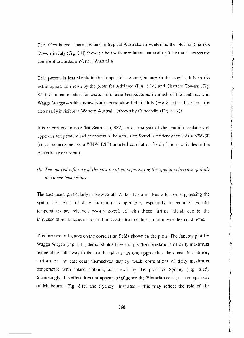
The effect is even more obvious in tropical Australia in winter, as the plot for Charters
Towers in July (Fig. 8.lj) shows; a belt with correlations exceeding 0.5 extends across the
continent to northern Western Australia.
This pattern is less visible in the 'opposite' season (January in the tropics, July in the
extratropics), as shown by the plots for Adelaide (Fig. 8.le) and Charters Towers (Fig.
8.1 i). It is non-existent for winter minimum temperatures in much of the south-east, as
Wagga Wagga- with a near-circular conelation field in July (Fig. 8.1 b)- illustrates. It is
also nearly invisible in Western Australia (shown by Cunderdin (Fig. 8.1 k)).
It is interesting to note that Seaman (1982), in an analysis of the spatial con·elation of
upper-air temperature and geopotenti al heights, also found a tendency towards a NW -SE
(or, to be more precise, a WNW -ESE) oriented correlation field of those variables in the
Australian extratropics.
(b) The marked il~fluence (d" the east coast on suppressing the spatial coherence of daily
maximum temperature
The east coast, particularly in New South Wales, has a marked effect on suppressing the
spatial coherence of daily maximum temperature, especially in summer; coastal
temperatures arc relatively poorly correlated with those further inland, due to the
influence of sea breezes in moderating coastal temperatures in otherwise hot conditions.
This has two influences on the conelation fields shown in the plots. The January plot for
Wagga Wagga (Fig. 8.la) demonstrates how sharply the correlations of daily maxitnum
temperature fall away to the south and east as one approaches the coast. In addition,
stations on the east coast themselves display weak correlations of daily maximum
temperature with inland stations, as shown by the plot for Sydney (Fig. 8.1f).
Interestingly, this effect does not appear to influence the Victorian coast, as a comparison
of Melbourne (Fig. 8.1c) and Sydney illustrates - this may reflect the role of the
168
r i
I
I (
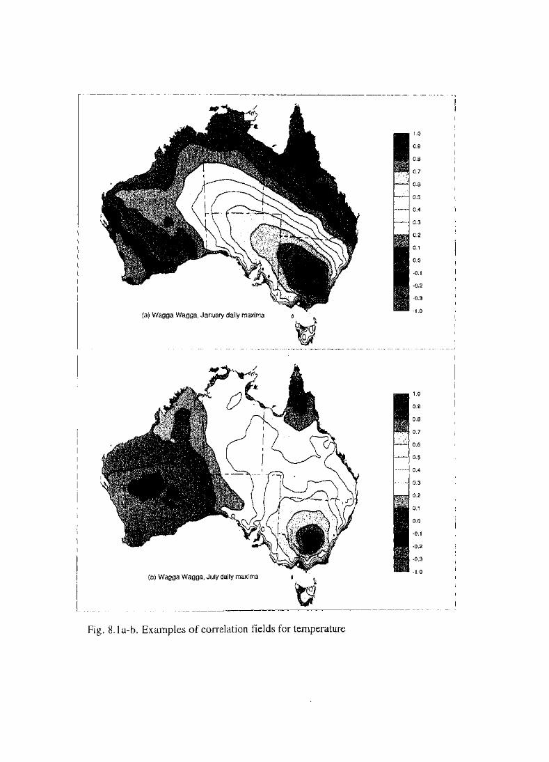
(a) Wagga Wagga, January dally maxima
(b) Wagga Wagga, July dally maxima
o~J v
Fig. 8.1 a-b. Exmnples of correlation fields for temperature
1.0
0.9
0.8
0.7
0.6
0.5
0.4
0.3
0.2
0.1
0.0
-0.1
-0.2
-0.3
-1.0
1.0
0.9
0.8
0.7
0.6
0.5
0.4
0.3
0.2
0.1
0.0
-0.1
-0.2
-0.3
·1.0
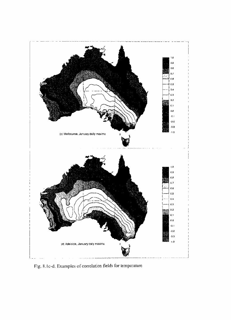
(c) Melbourne, January daily maxima
(d) Adelaide, January daily maxima
Fig. 8.1 c-d. Exan1ples of correlation fields for temperature
1.0
0.9
0.8
0.7
0.6
0.5
0.4
0.3
0.2
0.1
0.0
·0.1
-0.2
-0.3
-1.0
1.0
0.9
0.8
0.7
0.6
0.5
0.4
0.3
0.2
0.1
0.0
·0.1
-0.2
·0.3
-1.0

(e) Adelaide, July daily maxima
"""~--·----------------------_j
(I) Sydney, January daily maxima
. --·"···---·---------------------------__J
Fig. X.l e- f. Examples of correlation fields for temperature
(g) Alice Springs, Jan. daily maxima
(h) Alice Springs, Jan. monthly maxima
Fig. 8.1 g-h. Examples of correlation fields for temperature
1.0
0.9
0.8
0.7
0.6
0.5
0.4
0.3
0.2
0.1
0.0
-0.1
-0.2
-0.3
·1.0
1.0
0.9
0.8
0.7
0.6
0.5
0.4
0.3
0.2
0.1
0.0
-0.1
·0.2
-0.3
·1.0

(i) Charters Towers, Jan. dally maxima
Ul Charters Towers, July daily maxima
Fig. 8.li-j. Examples of correlation fields for temperature
1.0
0.9
O.B
0.7
0.6
0.5
0.4
0.3
0.2
0.1
0.0
-0.1
-0.2
-0.3
-1.0
1.0
0.9
0.8
0.7
0.6
0.5
0.4
0.3
0.2
0.1
0.0
·0.1
-0.2
-0.3
-1.0

(k) Cunderdin, January daily maxima
Fig. 8.lk. Examples of correlation fields for temperature
1.0
0.9
0.8
0.7
0.6
0.5
0.4
0.3
0.2
0.1
0.0
-0.1
-0.2
-0.3
-1.0

(I) Darwin, January daily minima
(m) Darwin, July daily minima
1.0
0.9
0.8
0.7
0.6
0.5
0.4
0.3
0.2
0.1
0.0
·0.1
-0.2
-0.3
·1.0
1.0
0.9
0.8
0.7
0.6
0.5
0.4
0.3
0.2
0.1
0.0
-0.1
-0.2
·0.3
·1.0
'-----------------------------------·---.,--··-----··---
Fig. 8.11-m. Examples of correlation fields for temperature

·mountain barrier inland from the New South Wales coast, which has only a limited
Victorian equivalent, in limiting the influence of hot air of inland origin on the coast. The
Cunderdin plot (Fig. 8.1 k) suggests a similar effect on the south coast of Western
Australia, but the station network is not sufficiently dense to resolve this with the smne
degree of confidence as is possible in New South Wales.
(c) The seasonal variation in the spatial coherence of daily minimwn temperatures in
tropical Australia
There is a very n1arked seasonal variation in the spatial coherence of daily minimum
te1nperature in tropical Australia. This is shown particularly strongly by the plots for
Darwin for January (Fig. 8.11) and July (Fig. 8.1m). In January, when low minimun1
ten1peratures occur principally as a result of downdrafts in thunderstorms - and are
consequently localised -Darwin shows very weak correlations with all stations outside
its i1nmediate region. Conversely, in July, when low minimum temperatures occur
principally in south-easterly surges - a broad-scale synoptic phenomenon - Darwin
displays strong (> 0.4) correlations with most of the region north of the Tropic of
Capricorn. A particularly striking contrast is that January minimum temperatures 111
Katherine display the san1e level of correlation with Darwin as do July minimum
temperatures in northern Victoria!
8.2.3. Variation between the correlation fields on the daily and monthly tin1escales
An example of the di {Terence between the correlation fields on the daily and n1onthly
timescales is shown by the plots for January maximum temperature at Alice Springs (Fig.
8.1 g, 8.1 h). The monthly mean temperatures show greater spatial coherence than the
daily temperatures, as one might expect, but differences and similarities in the nature of
the fields are of interest. The most substantial differences between the two fields are that
monthly mean te1nperatures on the Queensland coast are quite strongly correlated (0.4-
0.6) with those at Alice Springs, whereas there is little or no correlation for daily
temperatures between the two regions; and that monthly mean te1nperatures in Victoria
169

and southern South Australia are much more weakly correlated with those at Alice
Springs. than daily temperatures are, reaching the extent that in western Victoria and the
far south-east of South Australia the daily temperatures are positively correlated with
those at Alice Springs, but for monthly mean temperatures the conelations are negative ..
This may reflect the role of the El Nino-Southern Oscillation in influencing temperatures
on the monthly timescale; it is interesting to note that the pattern of correlations of
monthly mean maximum temperatures with those at Alice Springs closely parallels the
pattern of their correlations with the Southern Oscillation Index (Jones, 1999).
A similarity between the monthly and daily timescales is that both display quite strong
negative correlations between Alice Springs and the west coast of Western Australia.
8.2.4. Calculation of the characteristic distance from a station at which correlations
fall to a certain level
An indicator of the spatial coherence of temperature in a region is the characteristic
distance at which the correlation of the temperature between pairs of stations falls to a
certain level.
This is determined by carrying out the following procedure for each station and month,
and for maximum and minimum temperature separately:
I. Analyse the correlations of all other stations with that station onto a I o by 1° grid,
using the Barnes analysis scheme initially described in section 4.2.3.
2. For each of the correlation thresholds 0.8, 0.6 and 0.4, find the number of grid
points where the analysed correlation exceeds the threshold.
170

3. Determine the proportion of land within the radius from the station at which the
correlation exceeds the threshold level. This is determined by finding, for each of
the 10 distances 1, 2, ... , 10 degrees (calculated as the Pythagorean distance,
treating the latitude/longitude grid as a regular grid, as previously defined in
Chapter 4) the proportion of land, and hence the land area (expressed as a number
of grid points), within that radius of the station. This gives a set of land areas
within a radius of 1, 2, ... , 10 degrees of the station.
4. Find the estirnated radius which cOITesponds to the number of grid points in step
2, by finding the pair of calculated land areas from step 3 which that number of
grid points lies between. (For example, if step 3 gives 140 land grid points within
7 degrees of the station and 170 land grid points within 8 degrees of the station,
and step 2 gives 155 grid points with a con-elation exceeding 0.4, this gives an
estimated radius between 7 and 8 degrees).
5. Find the proportion of land within the estimated radius of the station by linearly
interpolating between the proportions found for fixed radii either side of the
estimated radius in step 3.
6. Find the 'equivalent land area' with correlations exceeding the threshold by
dividing the nun1ber of grid points found in step 2 by the proportion of land within
the estimated radius found in step 5. This step has the effect of nominally
extending the region of cOITelations over a threshold over the ocean.
7. Find the characteristic radius of a certain correlation by finding the radius of the
circle which has the area of the 'equivalent land area' in step 6.
Maps of the characteristic radius of the 0.4 correlation for each of four rnid-season
n1onths (January, April, July and October), adopted as a broad indicator of the spatial
coherence of the variables under examination, are displayed for daily temperature data in
Figs. 8.2a (maximum temperatures) and 8.2b (minima), and for n1onthly data in Figs. 8.3a
and 8.3b. The full list of characteristic radii of the threshold correlations for each station
are listed in Appendix E (Tables E.1a-d).
171

h 1 1 the regional and seasonal variations in the spatial c.:ohcrcnce' These maps s ow c ear Y
d"f:C b tween the spatial coherence or ft.~tnpl·raturc nn temperature, and the I lerences e
daily and monthly timescale.
Daily maximum temperature
The characteristic radius of the 0.4 correlation for daily maxi mum ternperatun.~ is
over most of Australia than that for daily minimum temperature. and shows less
variation, although values are generally lower in summer than \\'inter. In wint1..~r' the
exceeds 1000 km over most of Australia, reaching 1400 km in parts of C)u«.~<.~nshmd
the Northern Territory, whereas in summer I 000 km is on I y reached ewer parts nf
inland south-east. The lowest values occur in summer on those L'nasts whL•n,•
have the greatest influence on maximum temperatures Nl'\v Snurh \Vales ~md
southern half of Western Australia- with 358 km being reached at ( 'arnarnm in 1 antHJW"~
Daily minimum temperature
The most striking result is the complete seasonal reversal in 1 he· gc()vraph tL' ;d pattern
the spatial coherence of daily minimum ternperaturL'. f'v1inirnurrJ rcrnpcrature shov .. ,s \\'i,''\.J!L
spatial coherence over most of northern Australia in SlllllflllT, \\ rtlt the charar:tcn~u..:"
radius of the 0.4 correlation below 500 km over most or tile tr()plL"s ;md L'loser to 300
in the far north, but in winter the radius exceeds I()()() k rn over a! most all uf this
(except for the Cape York Peninsula), and reaches 1~21 krn at Darw1n. (T!Jis IS cnnsis.h::ru
with the correlation fields for Darwin displayed in hgs. K. II and K.ln1 ). I·:\'L~n fllUi'ffl:'
strikingly, using Darwin as an example, much or the shirt takes plaL'L' in a single: nmnth
the radius increases from 678 km in April to 1630 km in May, then deL'!"t:ascs ff'()tll 11
km in September to 428 km in October. This behaviour aprx~ur:-; to n:rlc:et the role
mesoscale phenomena, such as thunderstorms, in influencing low rninimutn tcn1peraturt.~ in the tropical wet season- radiational cooling at night is not the influence on rninin1um
temperatures here that it is elsewhere in Australia. Southern coasts display the oppo~ute pattern, with the characteristic radius having a summer maxirnurn und winter minimurn,,.
172

1 3000 3000
1800 1800
1600 1600
1400 1400 1200 1200
1000
800
600 400
200
January ,. . -0
3000 3000 1800 1800 1600 1600
1400 1400 1200 1200
1000 1000
800 800 600 600
400 400
200 200
July ., -0 October 0 ;
" !
\ ;._
Fig. 8.2a. Characteristic radius of correlations - daily maximum temperature

1 I
3000 3000 1800 1800 1600 1600 1400 1400 1200 1200
1000 1000 800
600
400
200
January "Y
! -o
3000 3000 1800 1800 1600 1600 1400 1400 1200 1200 1000 1000 800 800 600 600 400 400 200 200
July "T -0 October 0 ' \
I \
Fig. 8.2b. Characteristic radius of correlations - daily minimum temperature
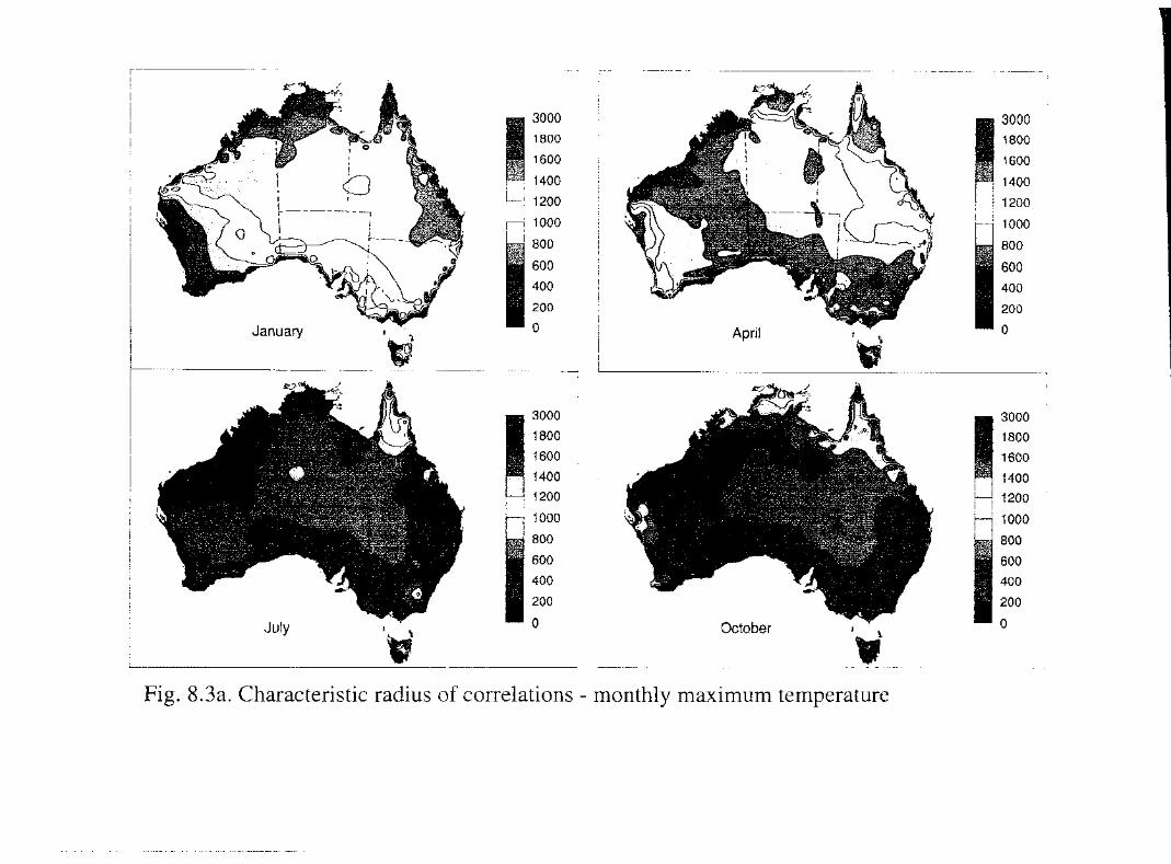
1 3000 3000 1800 1800 1600 1600
1400 1400 1200 1200 1000 - 1000
800 800
600 600 400 400 200 200
January "T ......... 0 0 I
3000 3000 1800 1800 1600 1600 1400 1400 1200 1200
1000 1000 800 800
600 600 400 400
200 200
July "T -o October 0
' \
Fig. 8.3a. Characteristic radius of correlations - monthly maximum temperature

3000 1 1800 I 1600 3000 1400 1800
1200 1600
1000 1400 800 1200
600
400
January , 200 s -o
3000 3000 1800 1800 1600 1600 1400 1400 1200 I
1200 1000 1000 800 800 600 600 400 400
200 200
July -. -0 October 0 : e \ c ~
Fig. 8.3b. Characteristic radius of correlations - monthly minimum temperature

>
although the contrasts are weaker (at Melbourne, the radius is 935 km in January and 576
km in July).
Monthly mean rnaximum temperature
Generally speaking, the monthly mean temperatures are more spatially coherent than
their daily counterparts. This is an expected result, as the statistical noise inherent in daily
temperatures would be expected to be reduced when averaged over a monthly mean. The
regional patterns of spatial coherence, however, differ considerably from those at the
daily timescale.
Monthly mean maxin1u1n ten1perature is the most spatially coherent of the variables
under consideration, with the characteristic radius of the 0.4 conelation exceeding 1000
km over the vast majority of Australia in all seasons, the only real exceptions being the
coasts of northern and western Australia at times in summer and autumn. The lowest
values occur on the coasts of Western Australia, with January values of 501 kn1 at Albany
and 450 km at Carnarvon.
During winter, the characteristic radius exceeds 1400 km over ahnost all of Australia, and
reaches 2000 km in northern New South Wales and southern Queensland. Even in
summer, it reaches 1600 kn1 in parts of the Northern Tenitory and Queensland, and
exceeds 1200 km away from the southe111 coasts. Inland southern New South Wales is a
region of strong spatial coherence of maximum temperature in all seasons.
Monthly mean minimum temperature
The largest values of the characteristic radius of the 0.4 COITelation occur during the
winter half-year, approaching 2000 km in parts of northern Australia during April and
July. 1100 km is exceeded over almost all of Australia in winter, except for the south
coast of Western Australia. The sharp drop in the spatial coherence of daily minimum
temperatures along the southern coasts from summer to winter has no counterpart at the
173

monthly timescale, although there is some evidence of a spring minimum there. On the
other hand, northern Australia shows a marked winter peak, as it does at the daily
timescale. Darwin shows very marked changes between months in spring and autumn, as
it does for the daily timescale, but the timing is slightly different Uumping from 875 km
in March to 2037 km in April, then dropping from 1454 km in October to 406 km in
November). This may reflect the strength of the main monsoon as an influence on mean
monthly temperatures in this region, while daily temperatures are influenced by
individual storm events, which take place over a slightly longer season.
As at the daily timescale, the characteristic radius is genera)]y shorter in western than it is
in eastern Australia.
A comparison with rainfall
By way of comparison, the spatial coherence of daily and monthly rainfall, using data
from the same stations as temperature, is displayed in Figs. 8.4 and 8.5. These show that
temperature shows substantially greater spatial coherence than rainfall. Monthly rainfa11
displays a characteristic radius of the 0.4 correlation which is generally of comparable
magnitude to daily temperature, while daily rainfall is even less spatially coherent, with
the characteristic radius rarely exceeding 600 km in any season.
8.3. The development of spatial averages of Australian extren1e temperature data
The following sections of this chapter are based on a set of 99 stations. This is the set of
high-quality temperature stations described in Chapter 3, without island and Antarctic
stations or the city locations in Sydney, Melbourne, Brisbane and Adelaide. Perth Airport
is retained in the set, despite some evidence of an artificial warming trend since 1970
(presumably resulting from urbanisation), because of the lack of a suitable substitute non
urban station to represent the coastal region of Western Australia between Geraldton and
Cape Leeuwin. As much of the available daily data commences in 1957, spatial averages
are calculated for each year from 1957 to 1996 inclusive. There is insufficient spatial
174
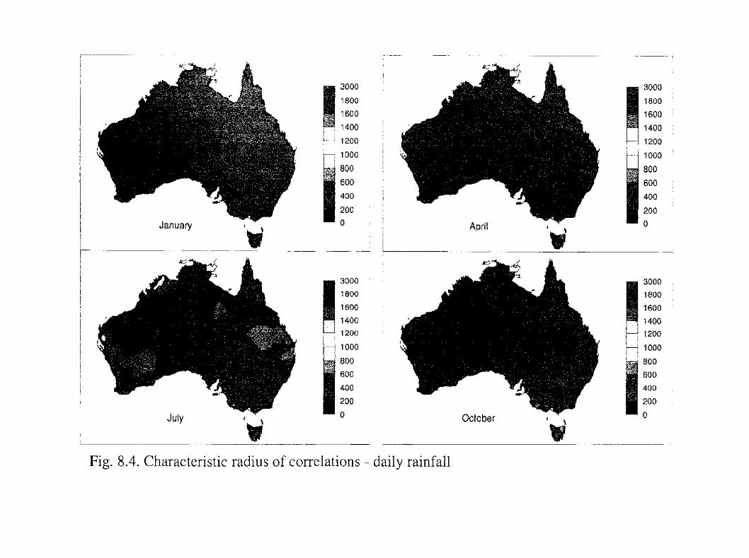
3000 3000 1800 1800 1600 1600 1400 1400 1200 1200
1000 j 1000 800 800 600 600 400 400
200 200
January ,. -0 0 .
3000 3000 1800 1800 1600 1600 1400 1400 1200 1200
1000 1000
800 800 600 600 400 400
200 200
July , -0 October I 0 \ '- \
Fig. 8.4. Characteristic radius of correlations - daily rainfall
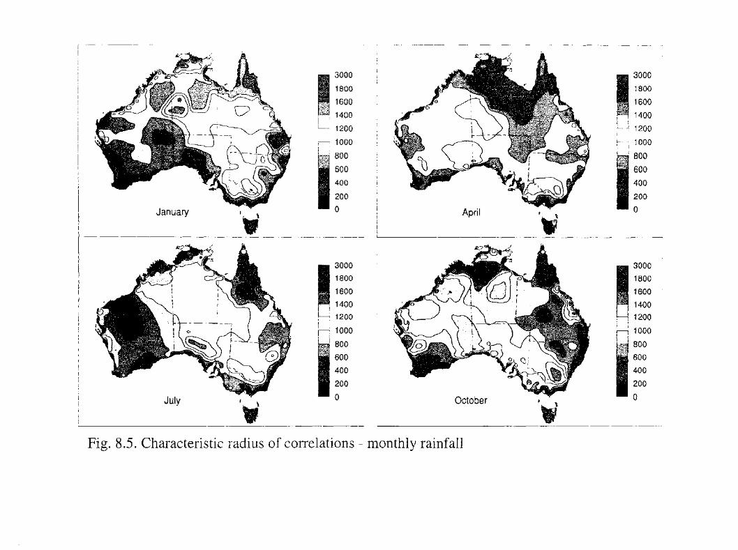
3000 3000
1800 1800
1600 1600
1400 1400
1200
1000
800
600
400
200
January "T -0
3000 3000
1800 1800
1600 1600
1400 1400 1200 1200
1000 1000
800 800
600 600
400 400
200 200
July • \ - 0 October • \ 0
Fig. 8.5. Characteristic radius of correlations - monthly rainfall
coverage prior to 1957 to allow the analysis to be extended back beyond that year (at
least until additional digitisation of manuscript data takes place).
8.3.1. Methods used in the development of spatial averages
The simplest possible method for calculating a spatial average is to take the arithmetic
mean of data frorn a representative sample of stations for the period of interest. Whilst it
is sitnple - and is the method used for the calculation of district average rainfalls for
Australia (Jones and Beard, 1998)- the inadequacies of this method are obvious. It takes
no account of changes in the density of stations (other than in the original choice of
stations, if the station network is sufficiently dense to allow a choice of stations within it),
meaning that areas with sparse station networks are under-represented in the results.
Jones and Beard (1998) found substantial differences between district average rainfalls
generated by this method and those generated by a more sophisticated gridding technique
(for example, the mean annual rainfall for district 97, in western Tasmania, is 2320 mm
in the conventional district series, but 1588 mm - 31%1 lower - using a grid-derived
series, because of the clustering of long-term stations in the wetter parts of the district),
while both they and Chappel ( 1995) found that changes in the station network in district
96 (central Tasmania) had led to an artificial increase in the district average rainfall in
this region, if a simple arithmetic rnean is used. Nicholls (2000) also found an artificial
negative trend in mean annual rainfall in district 71 (Snowy Mountains), due to the
closure or two stations in the wettest part of the district.
This deficiency was first recognised by Thiessen ( 1911 ), who developed a method of
dividing a region into polygons by drawing lines equidistant from each member of a pair
of neighbouring stations (the polygons thus produced contain all points that are closer to
the station within that polygon than to any other). The spatial mean - of precipitation, in
the case of Thiessen's paper- was then calculated by weighting the value at each station
by the area of its associated polygon. This is now known as the Jnethod of Thiessen
polygons.
175
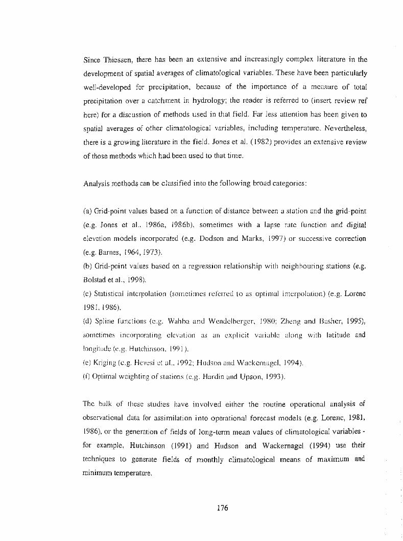
Since Thiessen, there has been an extensive and increasingly complex literature in the
development of spatial averages of climatological variables. These have been particularly
well-developed for precipitation, because of the importance of a measure of total
precipitation over a catchment in hydrology; the reader is referred to (insert review ref
here) for a discussion of methods used in that field. Far less attention has been given to
spatial averages of other climatological variables, including temperature. Nevertheless,
there is a growing literature in the field. Jones et al. (1982) provides an extensive review
of those methods which had been used to that time.
Analysis methods can be classified into the following broad categories:
(a) Grid-point values based on a function of distance between a station and the grid-point
(e.g. Jones et al., 1986a, 1986b), sometimes with a lapse rate function and digital
elevation models incorporated (e.g. Dodson and Marks, 1997) or successive coiTection
(e.g. Barnes, 1964, 1973).
(b) Grid-point values based on a regression relationship with neighbouring stations (e.g.
Bolstad et al., 1998).
(c) Statistical interpolation (son1eti1nes referred to as optimal interpolation) (e.g. Lorenc
1981, 1986).
(d) Spline functions (e.g. Wahba and Wcndclbcrger, 1980; Zhcng and Basher, 1995),
sometimes incorporating elevation as an explicit variable along with latitude and
longitude (e.g. Hutchinson, 1991 ).
(e) Kriging (e.g. Hevcsi ct al., 1992; Hudson and Wackernagcl, 1994).
(f) Optimal weighting of stations (e.g. Hardin and Upson, 1993 ).
The bulk of these studies have involved either the routine operational analysis of
observational data for assirnilation into operational forecast tnodels (e.g. Lorenc, 1981,
1986), or the generation of fields of long-term mean values of climatological variables
for example, Hutchinson (1991) and Hudson and Wackernagel (1994) use their
techniques to generate fields of monthly climatological means of maximum and
minimum temperature.
176

Those studies which have compared methods in specific situations have, in general,
found relatively small differences between techniques. Jones and Trewin (2000b), in an
examination of the efTecti veness of the Barnes successive correction technique, statistical
interpolation and thin-plate splines, found that, whilst statistical interpolation (SI) was the
rnost effective (in the sense of producing the lowest root-mean-square (RMS) average
error) of these methods for the interpolation of mean monthly maximum and minimum
temperatures over Australia, the differences between the techniques were small (the RMS
errors for the Sl technique were 0.52°C for maxi1na and 0.55°C for minima, compared
with 0.(>1 oc and 0.62oC respectively for the Barnes scheme). Small differences were also
found bet ween kriging and a technique based on simple inverse-distance weighting and a
I apse rate function by Do<.lson and Marks (1997), whilst Bolstad et al. ( 1998) found a
regression-based technique pcrforn1ed better than kriging for their data set, noting that
kriging did not perform well where data were sparse.
(;. j vcn the small di rrercnccs round between techniques, and the small differences in
computational efficiency between the Barnes sche1ne, SI and splines (D. A. Jones, pers.
cornn1. ), it was decided to test the Barnes scheme (as the system that is in operational use
v.:ithin the Australian National Climate Centre), along with three schemes which were
rnuch more computationally sitnple and had been used previously for the compilation of
large sets ol' spatial averages:
•
•
•
Thiessen polygons (Thiessen, 1911)
The method of Shepard ct al. ( 1968)
The method of Jones et al. ( 1986a, b)
177

8.3.2. Specific methods used in this study
8.3.2.1. The Jones method
This method was used by Jones et al. (1986a, b) in the development of a global data set of
monthly mean temperatures on a grid of 5° latitude by 10° longitude.
Each station is associated with its nearest grid point (i.e. each station only influences the
value at one grid point). For each grid point, the monthly mean temperature anomaly of
all stations associated with that grid point is averaged, with the value from each station
weighted using the weighting function:
where di =the distance between the station and the gridpoint or 50
nautical miles, whichever is the greater
(the 50 nautical miles condition being added to prevent problems arising when a station is
very near the gridpoint).
The global mean temperature anornaly is then calculated as the arithmetic mean of the
value at all grid points. This method uses distance as the sole criterion for the weight that
a station carries in the calculation or the station mean.
8.3.2.2. The Shepard n1ethod
This method, like the Jones method, associates each data point with a single grid point.
However, in addition to using distance as a criterion for the weight a station carries,
Shepard's method uses a measure of the angular density of stations. The principle used is
that the data in each direction from a grid point should carry equal weight in the
calculation of a value at that grid point. Accordingly, the method gives lesser weight to
the data fr01n stations which are clustered in the same direction from a grid point than it
178

does to data fron1 a isolated station which ts the same distance away m a different
direction.
The algorithm used is that the weighting function, hi, at station i is given by:
bi == ( 1 + a;) (w/ ), where a; and wi are calculated as follows:
w; = 1/d, d < 133.3 km
= [ (6.75/d)((d/400- 1 )2) J, d > 133.3 km, where d =distance (km) between station
i and grid point
I! L WJ(cos({J -Q)) a;,= --=-J-=I _____ _
II
"w LJ' .H
where Oi represents the direction of station i from the grid-point concerned.
8.3.2.3. Barnes analysis
This is a successive-correction scheme, which was introduced in section 4.2.3. The grid
point values arc based on <.lata from nearby observation points; however, unli kc the Jones
and Shepard methods, an observation can inlluence the value at more than one grid point.
The analysis is performeu in four iterations, with the weighting function adjusted such
that the nearest observational data are given greater weight in the later iterations, thus
reducing the di ffercnce between the grid and observed data. The usc of a given
observation at more than one grid point makes it feasible to carry out this analysis scheme
on a much finer grid resolution than the Jones and Shepard methods. In this study it was
caJTied out at grid points separated by 1 degree in both latitude and longitude (compared
with 5 degrees for Jones and Shepard).
179

This is the scheme currently used for the production of operational analyses of climate
data in the Australian Bureau of Meteorology.
As introduced in section 4.2.3, the algorithm for the n-th iteration at a grid-point (i,j),
t,J i,j), is given by:
N L w(d)(T(s)- T(x(s), y(s)))
tn(i, }) = f(n -n(i, }) + ...::..s=--:.1----N------
LW(d) s=l
d2 w(d) = exp(loge(0.5)--
2 )
gnD
where: T( s) is the observed value of the analysed variable at stations
T(x(s),y(s)) is the value, interpolated from the analysis, of the analysed
variable at the position of stations, with co-ordinates (x(s),y(s))
dis the distance of station 5' from the grid point ( i,j)
D and g11 are constants which determine the effective length scales (the
distance at which the weighting function becomes 0.5) for each iteration
or the analysis
The constants are given the values:
D 500 km
gl 1.00
g2 0.36
g] 0.04
g4 0.04
180

which correspond to those used by the National Climate Centre in the routine analysis of
temperature. These values correspond to effective length scales of 500, 300, 100 and 100
kilometres respectively.
If the value of w(d) was less than 0.0001 then it was set to zero. At some grid points in
remote areas no station had a value of w(d) greater than 0.0001 on the third and fourth
pass. In this case t4(i,j) = t3(i,j) = t2(i,j) (i.e., in effect the third and fourth passes were not
run at these points and the value at the grid point was taken as that from the broader-scale
first and second passes).
8.3.,3. Advantages and disadvantages of the analysis and spatial averaging schemes
No spatial averaging or interpolation scheme is perfect; to achieve a perfect spatial
average would require the use of a set of stations which perfectly represented all of the
var:iations in the field being n1easurcd over a given region. A further consideration, albeit
one which is becoming less important as computing power becmnes cheaper and more
accessible, is that two of the schen1es outlined above, the Barnes and Thiessen schemes,
are quite computationally intensive when used with a varying station network, as will be
detailed further below.
Specific areas of interest include:
1. Representativeness rd' t lze interpolation/averaging
In three of the four schemes above, distance is, in effect, used as the sole measure of how
representative an observation at a station is of the actual conditions at some point. The
sole exception is the Shepard scheme, where the relative density of stations in a given
direction from the point is also given weight.
We have seen, in section 8.2, that there are 1narked variations over Australia in the spatial
coherence of temperature, and, in particular, that summer maxiinutn ten1peratures display
181

far less spatial coherence near some coasts than they do further inland. We have also seen
in that section that, in many cases, temperatures at a given site are much more strongly
correlated with those at a site in one direction than with one the same distance away in
another direction; examples include the tendency, already described, of maximum
temperatures in much of southern Australia to be more strongly correlated along a NW
SE axis than a NE-SW one, and that coastal sites on the New South Wales coast tend to
be more strongly correlated with each other than with inland sites, even if the inland sites
are closer.
The effect of these factors is that most distance-based interpolation or averaging schemes
tend to 'project' the influence of coastal sites further inland than is climatologically
justified. As an example, Bathurst is almost equidistant from Sydney and Dubbo, and
hence a distance-based interpolation scheme would give Sydney and Dubbo equal weight
in the estimation of conditions at Bathurst; however, the correlation of January maximum
temperatures at Bathurst with those at Dubbo is 0.91, while that of Bathurst and Sydney
is 0.50.
The use of statistical interpolation would alleviate some of this I ack of representativeness,
in as much as its usc of a two-dimensional covariance function allows observations in
some directions to be given more weight than those in others. This type of function would
allow adjustments to be made for the ohservecl NW-SE axis of strong corTelations. In its
usual form, however, the covariance function over a field rernains independent of the
location of the origin and its value depends only on the vector displacement of a point
from the origin. This docs not allow the taking into account of the influence of the coast
at near-coastal sites, nor the rnarked latitudinal and seasonal variations in the spatial
coherence of temperature described in section 8.2. Attempting to extend and adapt the
concept of statistical interpolation to cover such situations is beyond the scope of this
thesis.
As all of the schemes discussed above are distance-based, none has a particular advantage
over the others in this respect. The directional weighting in the Shepard scheme only
182

takes into account the density of stations in a given direction, and is designed to give
practical effect to the intent to weight data from all directions equally, without the
distortions caused by varying numbers of stations.
2. Computational simplicity
The simplest schemes computationally, by some margin, are the Jones and Shepard
schemes, as both allow observations to influence the value at one grid point only, and use
a relatively coarse grid. The Jones method is particularly simple as it uses a single
distance-based calculation to determine the weight that any observation plays at a grid
point.
In a complete data set, the Thiessen method is also computationally simple, as the 1nost
con1putationally complex part of the calculation, determining the area of the polygons
associated with each data point, only has to be carried out once. In a real data set, the area
of the polygons has to be recalculated every time the station network changes- that is, on
every occasion that there is missing data at one of the stations. This adds considerably to
the computational demands.
The Barnes scheme is the n1ost cornputationally complex, because of its finer grid
spacing- 1 o instead of 5°, as in the Jones and Shepard schemes- and because it uses four
iterations at every grid point. The finer resolution is not inherent to the schemes per se,
but is a consequence of the fact that the Jones and Shepard schemes only allow an
observation to be associated with its nearest grid point, which in turn would result in no
value being defined at many grid points if a resolution of finer than 5° were to be used.
The size of the data set used in this part of the study (99 stations) was sn1all enough for
Barnes analysis to be able to be run without undue difficulty, so computational simplicity
was not a significant factor. It would become more itnportant in a global data set in which
several thousand stations were involved, the type of data set for which the Jones
algorithm was specifically designed.
183

3. Detail of analysis
As a result of the constraint that no data point may influence the value at more than one
grid point, the Jones and Shepard methods are effectively limited to a relatively coarse
grid. The global analysis of Jones et al. (1986a, b) is run on a grid of so latitude by 10°
longitude. In this study a so by so grid is used. This is the smallest spacing feasible in
order for most g1id points to have at least one station associated with them; even so, there
are three grid points in Western Australia with which no station is associated (i.e. there is
no station within 2.5° in any direction). National averages can be calculated on this scale,
but any finer-scale breakdown is difficult. In particular, on this scale no grid point lies
within Victoria or Tasmania.
The Barnes scheme is run at a I 0 by I 0 resolution. This is feasible because of the use of
the data from each station at multiple grid points. It could be argued that this grid scale
gives a level of detail in remote areas that is not justified by the sparseness of the data.
The strong spatial coherence of temperature in these regions, though, should minimise
any distortions caused. The fine scale of the analysis makes it feasible to calculate state
by-state averages, although these are subject to their own distortions (see section 8.4).
8.3.4. An objective assessment of the spatial averaging techni(JUCS
To present a case study of the consistency and bias or the spatial averaging techniques,
the Australia-wide average or the number of days with mininw below ooc was calculated
for each year between 1957 and 1 996.
Table 8.1 shows the mean number of such days calculated using each of these techniques
for the 40-year period, while Table 8.2 shows how well-conelated the results from each
technique are with each other. These results show that, on the annual timescale, the
results from the four methods are extremely well-correlated (r > 0.977), and hence any of
the four are essentially consistent in their representation of interannual variation of the
frequency of days with minima below 0°C.
184

The mean annual number of days, averaged over Australia, with minima below ooc is
calculated as being 10% greater using the Jones method than the Thiessen method, to take
the two extremes. These reflect opposite biases in the two methods. The Jones and
Shepard methods effecbvely exclude three Western Australian grid points, as noted in
section 8.3.3, because of a lack of nearby data, and therefore give additional weight to the
other Australian grid points- in particular, those in south-eastern Australia where mini1na
below ooc are most frequent. (This bias would be more substantial for high maximum
ternperatures, as these are I ikely to be frequent at all of the three grid points in question).
Conversely, the Thiessen method effectively gives each point the value of its nearest
station, extending the inl1uence of coastal stations to the point inland that is equidistant
between the coastal station and the nearest inland station. As most coastal stations rarely
or never record 1nini1na below 0°C, this reduces the calculated tnean frequency of such
events. (The other methods also project coastal observations inland, but the inland
observations still have some influence, even at near-coastal grid points).
The results shown in Tables 8.1 and 8.2 suggest that, for this particular case, it docs not
greatly matter, in the representation of the frequency of extreme temperature events,
which of the four methods is chosen. The Barnes method is therefore used for the
remainder of the analysis, because of its greater level of spatial detail.
8.4. Spatial averages of the frequency of extren1e tentperature events
8.4.1. Which extren1e events should be analysed?
The question or whether to use fixed or percentile-based thresholds for the analysis of
extreme events has been previously been discussed in Chapter 7, and the advantages and
disadvantages of both were discussed there. In the context of spatial averages, fixed
thresholds suffer from two particular disadvantages:
185

1. Impact of changes in station network
The station network is not static; many stations miss days on an irregular basis, and some
were not open for the entire 1957-1996 period. This biases the spatial averages in
situations where the station whose data are missing is significantly warmer or colder than
its neighbouring stations. If a station's data are missing the values at neighbouring
stations will effectively be interpolated to that station, thus producing a bias in the record.
The Tasmanian data shown in Fig. 8.6 illustrate this point. The Butlers Gorge station
closed in 1993, and its data are therefore not included in the averages for 1994-1996. As
Butlers Gorge has a much greater frequency of minima below ooc than any other
Tasmanian station (Table 8.3, station nun1bers 91 000-99999), its removal will cause a
sharp downward bias in the calculated mean number of days below 0°C. The absence of
Cabramuna (opened 1962) from 1957-61 data has a similar impact on the frequency of
low maximum temperatures (not shown).
2. Lack of areal representativeness r~l station network
Many fixed-threshold extreme events arc only observed in parts of Australia, or are
observed with a much greater frequency at some stations than others. Table 8.3 shows an
example of this, the frequency of minima below ouc at all stations within Australia. It
may be seen that there are only nine stations in the data set which record a mean of more
than 20 nights per year with minima below 0°C, and five with 50 or more such nights.
The interannual variability of the all-Australian average is therefore likely to be
dominated by changes at these sites. As a result, a figure purporting to be an all
Australian average is dominated by a few sites in a particular region of the country,
which is clearly not an especially representative outcome.
Furthennore, spatial averages of breaches of fixed thresholds will be dominated by events
in one season; summer for high thresholds, winter for low thresholds. To gain an
186

Table 8.1. Mean number of days with minima below ooc over Australia, using differing spatial averaging techniques
Technique Mean number of days per year below 0°C
Thiessen 3.99 Jones 4.55 Shepard 4.28 Barnes 4.38
Table 8.2. Correlations of annual frequency of minima below o<>C using different spatial averaging techni<Jues
Technique Technique Thiessen Jones Shepard Barnes
Thiessen 1.000 0.977 0.978 0.988 Jones 0.977 1.000 0.993 0.987 Shepard 0.978 0.993 1.000 0.991 Barnes 0.988 0.987 0.991 1.000

Fig. 8.6. Frequency of minima below 0 degrees C, Tasmania
10
9
8
7
6 >. (.) c: Q) :::1 5 C" Q) .;: ~
4
3
2 -----
0+,--------~------------------------------------------------------------------------~--------~
1955 1960 1965 1970 1975 1980 1985 1990 1995 2000
Year

Table 8.3. Mean frequency of minima below 0°C at stations used in study
Station Station name Frequency Station Station name Frequency number (days/year) number (days/year)
01021 Kalumburu 0.0 39128 Bundaberg 0.0 02012 Halls Creek 0.0 40004 Amberley 5.9 03003 Broome 0.0 40223 Brisbane AP 0.0 04032 Port Hcdland 0.0 40908 Tewantin 0.0 05007 Lear month 0.0 42023 Miles 18.2
05026 Wittenoom 0.0 43034 St. George 1.6
06011 Carnarvon 0.0 44021 Charleville 12.1
07045 Mcekatharra 0.0 45017 Thargomindah 1.4 08039 Dalwallinu 0.2 46037 Tibooburra 1.7 08051 Gerald ton 0.0 46043 Wilcannia 4.6
09021 Perth AP 0.1 48027 Co bar 1.7
09518 Cape Lceuwin 0.0 48239 Bourke 2.0
09741 Albany 0.0 52088 Walgett 5.2
09789 Esperance 0.0 53048 Moree I 1.5
10035 Cunderdin 0.5 55024 Gunncdah SC 3.5 10648 Wandering 19.2 56017 Invcrell PO 59.9
11052 Forrest 4.2 58012 Yamba 0.0
12038 Kalgoorlie 4.6 59040 ColTs Harbour 0.7
13017 Giles 0.4 60026 Port Macquaric 0.0
14015 Darwin 0.0 61078 Williarntown 0.8
14825 Victoria River Downs 0.3 61089 Scone SC 4.7
15135 Tennant Creek 0.0 63005 Bathurst ARS 58.6
15548 Rabbit Flat 3.1 65012 Dubbo 15.1
15590 Alice Springs 11.8 66062 Sydney RO 0.0
1600 I W<HJmcra 0.1 67105 Richmond llJ
16044 Tarcoola 5.6 68034 Jervis Bay 0.1
1703I Oodnadatta 1.3 68076 Nowra 0.1
17043 Marrec 2.5 69018 Moruya Heads 0.1
18012 Ceduna 3.8 70014 Canberra Airport 61.4
18070 Port Lincoln 0.0 72161 Cabramurru 104.8
21046 Snowtown 5.5 72150 Wagga Wagga 22.0 22801 Cape Borda 0.0 73054 Wyalong 16J
23090 Auclaiuc RO 0.1 74128 Deniliquin 8.2 23321 Nuril lotpa 11.0 76031 Mildura 3.9
2(J02l Mount Gambier 5.7 78031 Nhill 13.4
2(J026 Rube 0.1 80023 Kerang 4.8
27022 Thursday Island 0.0 82039 Ruther glen 43.2
27045 Weipa 0.0 84016 Gabo Island 0.0
28004 Palmervil k 0.0 84030 Orb<lst 3.7
29004 Burketown 0.0 85072 Sale 12.3
30045 Richmond 0.3 85096 Wilsons Promontory 0.0
3101 I Cairns 0.0 86071 Melbourne RO 1.5
32040 Townsville 0.0 87031 Lavcrton 5.0
33lll9 Mackay MO 0.0 90015 Cape Otway 0.0
34084 Charters Towers 0.0 91057 Low 1·-Iead 0.3
36007 Barcaldine 0.6 91104 Launceston AP 28.7
36031 Longreach 1.4 92045 Eddystone Point 0.0 37010 Camooweal 0.2 94010 Cape Bruny 0.3
38002 Birdsville 0.2 94029 Hobart RO 1.6
38003 Boulia 0.0 94069 Grove 40.8
39039 Gayndah 2.6 96003 Butlers Gorge 91.2
39083 Rockhampton 0.1

indication of changes in frequency of extreme events through the year as a whole, a
broader measure is needed.
The principal method used in this study to analyse spatial averages of threshold event
frequency involves the use of percentile thresholds, that is, temperatures (maximum and
1ninimum) above the 90th and 95th percentile level for a calendar month, or below the
1Oth and 5th percentile level. The major advantage of this method is that the expected
frequency of such events is exactly the same- 5% or 10% (depending on the threshold
chosen) - for every station and season, so the removal of a station from the network or
the choice of a season will not result in an intrinsic bias in the outcmne. This is the
approach being followed by the WMO Com1nission for Climatology Climate Change
Detection Methodologies and Indices task group (Plummer, pers. comm.).
8.4 .. 2. Method of calculation of the percentile thresholds
Percentile thresholds in each month for each station are calculated as per the method
outlined in the analysis of individual stations in section 7.1.1. Once the thresholds are
calculated for each of the 12 months, the number of ti1nes that threshold is breached in
each month of the 40 years was calculated. This gives, for each station and threshold, a
40-year time series of monthly data for each of the four thresholds for minimum and
n1axin1un1 temperature. The spatial averages of the threshold event frequencies were then
calculated for each month of the 40-year period using the Barnes analysis technique, as
described in section 8.3 .2.4.
8.4.3. Trends in spatial averages of the frequency of extrerne ten1perature events
The results of an analysis of spatial averages of the frequency of extreme temperature
events are presented in Tables 8.4 to 8.7 and Figs. 8.7 to 8.10. Each of the types of event
analysed are discussed separately in this section.
187

8.4.3.1. High maximum temperatures
Over the period from 1957 to 1996, an increase of 21 o/o (1.7 days/decade), as derived
from the trend in a linear regression of the data, has occurred in the frequency of
maximum temperatures above the 90th percentile in Australia. This increase is observed
in all seasons, but is most marked in winter (29%) and least marked in autumn (12%).
The upward trend is not constant, but, as may be seen from Fig. 8.7a, reflects the
existence of two distinct periods of relative stability in the record, with a sharp jump
between the two in the late 1970's. The question of whether this can be explained, in part,
by the influence of an increased frequency of El Nifio events will be addressed in Chapter
9.
An upward trend has occurred in all states, although it is minimal in New South Wales
and Victoria. The most marked trends are found in Tasmania, especially in autumn and
winter, in which the frequency of maxima above the 90th percentile has increased by
58% over the 40 years. Fig. 8.7g shows that this largely reflects the occurrence of a
number of very warm years during the I 980's.
8.4.3.2. High minimum temperatures
Over the period from 1957 to 1996, an increase of 32C7~) (2.5 days/decade) has occurred in
the frequency of minimum temperatures above the 90th percentile in Australia (Fig.8.8a).
The most marked increases ( 40-41 (Yr1) arc observed in spring and autumn, with lesser
increases in summer and winter. Even more so than the frequency of high maximum
temperatures, the frequency of high minimum temperatures shows a marked jump in the
late 1970's, between two periods of relative stability.
The trends are strongest in north-eastern Australia, with New South Wales and
Queensland displaying ]ncreases in excess of 30%. Queensland has shown an increase in
frequency of these events of SOo/o, with strong trends in all seasons, but especially in
autumn. Increases in spring and autumn are observed everywhere, but Queensland and
188

Region Spring (Sep- Summer (Dec- Autumn (Mar- Winter (.Jun- Annual Nov) Feb) May) Aug)
Days/ % Days/ IJ'c, Days/ l!f, Days/ (J1, Days/ % decade change decade change decade change decade change decade change
1957- 1957- 1957- 1957- 1957-1996 1996 1996 1996 1996
Australia 0.4 19 0.4 19 0.3 12 0.6 29 1.7 21 NSW -0.1 6 0.2 10 -0.2 -7 0.3 16 0.2 2 Victoria -0.1 5 -0.3 -12 0.5 25 0.4 18 0.5 5 Queensland 0.3 17 1.0 57 0.3 17 0.6 26 2.2 28 S. Australia 0.5 25 0.9 50 0.5 25 0.5 25 2.5 32 W.Australia 0.3 17 0.1 4 0.4 19 0.7 36 1.5 !9 Tasmania 0.3 16 0.0 - [ 1.2 75 1.3 83 3.0 39
·- - ----~--- ~ ~·~" ~--~·---" ~-----·· --~---~
Table 8.4. Trends in frequency of maxilna above 90th percentile
Region Spring (Sep- Summer (Dec- Autumn (Mar- Winter (Jun- Annual Nov) Feb) May) Aug)
Days/ 1]1, Days/ ()1, Days/ 11(, Days/ (Jc, Days/ 'if, decade change decade change decade change decaJc change decade change
1957- I 957- !957- I 957- 1957-199(> 1996 !996 1996 199(> --
Australia 0.8 41 0.4 19 0.7 40 0.4 21 2.5 32 NSW CU 16 0.7 36 0.9 50 0.7 40 2.7 35 Victoria 0.() 2(> -0. [ -2 0.5 23 0.6 26 1.7 20 Queensland 0.9 51 0.8 43 1.2 68 0.6 32 3.(> 50 S. Australia 0.4 21 0.1 7 0.6 3 [ 0.2 10 1.5 [ 8 W.Australia fHi 48 0.2 10 0.4 !9 OJ 16 1.8 22 Tasmania 0.(> 25 -0.2 -8 0.6 25 0.1 6 l.l 12
-·------------------- --------~---
Table 8.5. Trends in frequency of minhna above 90th percentile

. •\u..,tralta :'\iSW \'1vtor ta
<.,ltll't'll~.lillld
S :\u•.tralttt \\'.1\u..,tralla
Ta•.rnama
......
Spring (Scp-NovJ
Days/ (~,
decade change 19:'i7-I<)<)(>
-O.J -D --0.2 .<)
.()) -:20 ().() -I .().<) -.1.1 .(),.1, -12 I.J -42 ....
Summer (Dec-Feb)
Days/ % decade change
1957-1996
-0.1 -2 0.0 I 0.2 10 -0.5 -I<) -!l.l 2 0.2 12 -OJ -14
Autumn (Mar- Winter (Jun-May) Aug)
Days/ % Days/ % decade change decade change
1957- 1957-1996 1996
-0.7 -25 -0.5 -19 -0.5 -19 -0.3 -14 -1.0 -35 -0.8 -29 -1.3 -41 0.0 I -0.8 -30 -1.4 -46 -0.4 -14 -0.3 -14 -1.5 -49 -0.7 -26
'I'ahle S.6. Trends in frequency of 1naxima below lOth percentile
:\11'>11 ;tiLt
'sw \i,(llft;t
<.,llll'l'II'•Lilld
,<.; :\t1•.tr ;lila
\\' :\u·,tiall;t
'Lt'dli;IflLI
Spnng ( SL·pNov)
. ~-·-·-l )ays/ % dcradl· chan gL'
(<))7
I <)t)( ) ·····I··
10 -·.17 O.H '.'\0 02 -7 lA -47 1.1, -42
.(),lJ ··.H O.H .. \0
Summer ~1),
Feb) Days/ % decade change
1957-19%
-0.7 -2(> 0.1 5 0. I 2 -1.2 -Jl) -0.7 -25 -0.5 -19 -0.5 -17
Autumn (Mar- Winter (Jun-May) Aug)
Days/ % Days/ % decade change decade change
1957- 1957-1996 1996
-0.5 -20 -1.0 -35 -0.7 -26 -1.2 -39 -0.8 -31 -0.5 -18 -1.4 -45 -1.5 -50 -0.6 -24 -1.2 -40 0.1 2 -0.6 -21 -0.8 -30 -0.5 -20
·ruble H.7. Trends in frequency of 1ninima below lOth percentile
Annual
Days/ % decade change
1957-1996
-1.5 -15 -1.0 -10 -2.1 -21 -1.8 -18 -3.2 -30 -0.7 -7 -4.0 -36
Annual
Days/ % decade change
1957-1996
-3.3 -30 -2.7 -26 -1.7 -17 -5.6 -47 -3.9 -35 -2.0 -20 -2.9 -27

(a) Australia
16r-----------------------------~
14
12
g 10
! 8.
'if. 6.
4
2
0+-----~----~----~------~--~
1950 1960 1970 1980 1990 2000
Year
(c) VIctoria
16 r-----------------------------~ 14.
12
~ 10
~ 8
l 6 'if.
4
2
0 ~----~-----r----~------r---~ 1950 1960 1970 1980 1990 2000
Yoar
(e) South Australia
18 .-------------------------------, 16
14
~ 12 r: ! 10
I a 'if. 6
4
2
0 ~----~----~----~------~--~ 1B50 1860 1970 1980 1990 2000
Year
(g) Tasmania
18 r-----------------------------~ 16
14
~ 12 c ! 10
l 8 'if. 6
4
2
0 ·~----~-----r----~------r---~ 1950 1960 1970 1980 1990 2000
Year
(b) New South Wales
20.-----------------------------~
18
16 14.
f 12
11~ ;1. 6
4
0·~----~----~----~-----r----~
1950 1960 1970 1980 1990 2000
Veer
(d) Queensland
20r-----------------------------~
18
16
114
12 10
8 ;1. 6
0~----~----~----~----~----~
1950 1960 1970 1980 1990 2000
(f) Western Australia
18r-----------------------------~
18
14
112
10
8
;1. 6
1950 1960 1970 1980 1990 2000
Year
(h) Northern Territory
25 .-----------------------------~
20
i 15
!10 5
0-~----r-----~----~----~----~ 1950 1960 1970 1980 1990 2000
Year
---------~----.... ---- .. _ .. ___________ .. _ .. _______________ 1----------------·-··------··------.. ---··----·-----
Fig. 8.7. Frequency of maxima above 90 percentile level

(a) Australia
18 r-------------------------------HI
14
j 12
10
fl
iJit fl
()
1~Jr,(J
11'1
14
1:.'
fw ! fi
fit (:\
"
HH!O 1~J70 1960 1990 2000
Year
(c) VIctoria
0 ~----~------~----~------r-----J 10'\f) 1~MIO 1070 1980 1990 2000
Year
(o) South Australia
li ~-----~------~----~------~--~ 1'1'>ll l•Hi!l 11170 1fJ(lO 1990 2000
Yo or
(g) Tasmania
1!1 ... "-------·----14
'J
IJ 1----...... ---...,....--.....,..---.------f 1~lM 1000 1970 1980 1990 2000
Year
(b) New South Wales
18r---------------------------~ 18
14
g 12
~ 10
I 8 11. 6
1960 1970 1980 1990 2000
Year
... ····----------------------!
(d) Queensland
20r---------------------------~
18 16
14 f 12
I 1~ 11. 6·
1950 1960 1970 1980 1990 2000
Year
------·----------------
(f) Western Australia
16r---~~-----------------------,
14 .
12
r: 1.1. 6-
1950 1960 1970 1980 1990 2000
Year
........ ----------------------------------1
(h) Northern Territory
20~------------------------------~
18 16
~ 14
~ 12 i' 10 . ~ 8 11.
4-
2
0-~----~----~----~------~----~ 1950 1960 1970 1980 1990 2000
Year
........... ___________ .L,_ ____________________ ____j
Fig. 8.8. Frequency of minima above 90 percentile level

(a) Australia
18r-------------------------------~
16
14
~ 12 c 8 10
I 8 ';1. 6
4·
1!350 1960 1970 1980 1990 2000
Year
(c) VIctoria
18 r-------------------------------~ 16
14
~ 12
! 10
I a ';1. 6
2
1!~50 1960 1970 1980 1990 2000
Year
(e) South Australia
20 r-------------------------------~ 18
16
~ 14 c: 12 <ll
! 1~ 'if.
4
2
0 ~-----r----~------T-----~----~ 1950 1960 1970 1!:180 1990 2000
Year
(g) Tasmania
18 r-------------------------------~ 16
14
~ 12 c: <I> 10
1 8
'if. 6
4
0 ~-----r----~------~----~----~ 1950 1960 1970 1980 1990 2000
Year
-----·---·--------------------··----
(b) New South Wales
16 .-------------------------------~ 14
12
~ 10 ! 8
1950 1960 1970 1980 1990 2000
Year
(d) Queensland
16r-------------------------------~
16' 14
112
10
6
.,. 6
1950 1960 1970 1980 1990 2000
Year
(f) Western Australia
20 r-------------------------------~ 18
18
J 14
12
10
8 ';1. 6
1950 1960 1970 1980 1990 2000
Year
(h) Northern Territory
25 r-----------------------------~
20
5·
1950 1960 1970 1980 1990 2000
Year
···-----------------·---·-- .... --·- ,, _, _______________ ,~__ ______ _
Fig. 8.9. Frequency of maxima below 10 percentile level
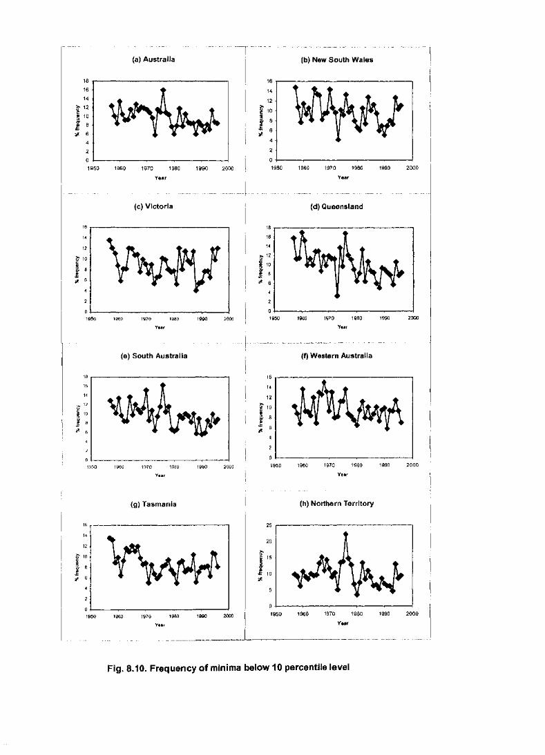
(a) Australia
18
16
14
~ 12 c: § 10 a'
8 .g ;J!. 6
4
2
0 1950 1960 1970 1980 1990 2000
Year
(c) VIctoria
1950 1000 1970 1960 1990 2000
Year
(e) South Australia
1Br--------------------------------, 10
14
!; 12
! 10
I e ;II.
1050
16
14
12
~ 10
~ I )1. 6
0
1950
1!Ki0
1000
---w~.~----·- -~ ~···~·-•-<>•" •-
1[170 1(180 1900 2000
Year
(g) Tasmania
1070 1960 1990 2000
Year
--·----.-···-··-----·-~-----
(b) New South Wales
16 r--------------------------------, 14 ..
12
f 10
I 8
7f. 6
4·
2
1950 1960 1970 1980 1990 2000
Year
{d) Queensland
16r--------------------------------,
16
14
~ 12
11~ )1. 6
1950 1960 1970 1980 1990 2000
Year
{f) Western Australia
16r-------------------------------~
14
1950 1960 1970 1960 1990 2000
Year
{h) Northern Territory
25
20
1" 10 ;J!.
0 ..
1950 1960 1970 1980 1990 2000
Year
----------·--·~---~----~·-·
Fig, 8.10. Frequency of minima below 10 percentile level
New South Wales are the only states to record more than minimal increases in summer.
The weakest trends through the year as a whole have occurred in Tasmania.
8.4.3.3. Low maximum temperatures
Over the period frmn 1957 to 1996, a decrease of 15%J (1.5 days/decade) has occurred in
the frequency of maximum temperatures below the lOth percentile in Australia
(Fig.8.9a). This is the weakest trend of the thresholds examined. It is most pronounced in
autumn and winter, with a decrease of 25% in autumn. There is virtually no trend in
summer. The trend for the annual data reflects the presence of four years in the record
( 1960, 1968, 1974 and 1978) with very high frequencies of days with maxima below the
lOth percentile. Apart from these four years, the frequency of such days has remained
virtually unchanged through the record.
The decline is tnost pronounced in southern Australia, particularly in autumn and winter.
South Australia and Tasmania have both observed large declines in the frequency of these
events. A possible cause for this change could be a change in the frequency of 'cold
outbreak' conditions over south-eastern Australia. The weakest trends are observed in
VVestern Australia, with an increase in the frequency of low maximum temperatures being
observed in summer.
8.4.3.4. Low ntininuun ten1peratures
Over the period from 1957 to 1996, a decrease of 30%J (3.3 days/decade) was observed in
the frequency of minimum temperatures below the lOth percentile level (Fig.8.10). This
is, by some margin, the most substantial trend observed of the threshold events examined.
The trends are strongest in winter and spring. The trend is a relatively consistent one
throughout the period of record (Fig. 8.10a), with the exception of a period of frequent
low minimum temperatures in the mid-1970's.
189

A decrease in the frequency of these events occurred in all states. The decline in
Queensland, which has occurred evenly throughout the year, is a particularly notable 47o/o
over the 40 years. Strong declines in winter and spring are observed in all states, except
for Victoria in spring. There was little trend observed in summer in New South Wales
and Victoria.
8.5. The preparation of a gridded data set of daily maximum and minimum
temperature
The preparation of meteorological data sets on a regular grid has been an active area of
interest, on both the global (e.g. Jones et al., 1986a, b) and national (e.g. Mills et al.,
1997) scales. It is an approach which, as discussed earlier, offers considerable advantages
in allowing data to be analysed on a consistent basis despite changes in station networks,
and in studying data spatially over specified areas, or over the globe. In particular, a set of
gridded daily temperature data for an extended period would allow an analysis of
variables such as the area over which a threshold is exceeded on any given day (for
example, the area over which 35°C is exceeded on each day of a period).
As has been the case with spatial averages (as described in 8.3.1), limited attention has
been given to griddcd analyses of daily temperature. The National Climate Centre of the
Australian Bureau of Meteorology has been producing griddcd analyses of daily
maximum and minimum temperatures for Australia since 1996, using the Barnes analysis
scheme. More recently, Janowiak and Bell ( 1999) have produced a set of gridded daily
maximum and minimum temperature data for the contiguous United States since 1948,
using (unadjusted) data from approximately 6000 co-operative stations and using the
analysis technique described in Cressman ( 1959).
The main purpose to which a gridded daily data set is put in this thesis is as an additional
tool in the quality control of the data, as described in Chapter 4. Its use for the analysis of
additional indices of extreme temperature values, beyond those previously discussed, is
beyond the scope of this thesis, but is certainly a potential area of study at a later date.
190

An important consideration in the generation of a gridded analysis of daily temperature
data is the station network to be used, and consequently the level of topographic detail
that is incorporated. One possible approach is to use all possible station data, no matter
what its period of record or quality. This approach would allow the maximum possible
level of detail to be obtained frmn station data, but would also induce numerous problems
with the lack of hmnogeneity through time of the analyses generated, as well as with the
effects of occasional erroneous or spurious data. This is not an intractable barrier for the
production of, for example, routine daily analyses for public information, but is a greater
problem if it is intended to use such a data set for the study of cliinate change. A more
subtle point is that some of the tnore extreme environments -for example, mountain tops
-are represented for only part of the period of record (a probletn also discussed in section
8.4.1. in the context of thresholds), and the use of station data alone would result in these
environments being lost frmn the record during periods when there are no data from those
stations. (To use a Tasmanian example, there have been data from high rnountain sites
above 1200 metres - Mount Wellington or Mount Barrow -only between 1961 and 1974
and since 1990, and hence Tastnanian station data would not allow the representation of
regions above 1200 tnctrcs between 1974 and 1990).
The problem or data hon1ogcneity can be addressed by using only data from known high
quality stations- in this context, the set of high-quality daily temperature data developed
earlier in this study. This, though, leaves a rather sparse network, with additional data
required in order to represent the full range of climates in Australia.
\Villmott and Robeson ( 1995) found that the most satisfactory results for the analysis of
temperature data were obtained by splicing anomalies from mean conditions, generated
from a particular set of data, onto a higher-resolution climatology developed using
additional data. Whilst their approach involved annual mean temperatures, there is no
reason why it could not be applied to shorter timescales. This is a particularly feasible
approach for Australian temperature data. High-resolution climatologies of monthly mean
ternperature in Australia have been developed by D. A. Jones (pers.comm .. ), using
191
techniques developed by Hutchinson (1991) to incorporate a wide range of station
temperature data, as well as high-resolution topographic models.
In this thesis, the data sets which were developed were daily anomalies from the mean
daily maximum and minimum temperature. These were interpolated onto a 1 x !-degree
grid using Barnes analysis, with the same parameters as described in section 8.3.2.3. This
was done separately for maximum and minimum temperature for each day from 1
January 1957 to 31 December 1996.
Examples of the data sets produced by this scheme are shown in Fig. 8.11. These show
the general spatial coherence of daily maximum and minimum temperature, except near
the coasts. The greatest problem in the development of such a data set is the sharp
temperature gradient near some of the coasts. While the use of anomalies in the gridding
process ameliorates this problem to some extent, the Barnes technique is still reliant on
the available station data. This means, using the case of 11 January 1957 for example,
that the data are approximately linearly interpolated between Kalgoorlie and Esperance
(in southern Western Australia), whereas it is likely, given the region's meteorology, that
there would be a rapid increase over the area immediately inland from Esperance,
followed by a levelling-out. This problem of capturing sharp gradients is inevitable
anywhere where the characteristics of the temperature field arc on a finer resolution than
the station network used to analyse it.
If these were to he developed into griddccl sets of daily maxtmum and minimum
temperature covering the same dates, a possi hie method would be to spl icc the daily
anomalies onto the high-resolution monthly climatology of Jones. To achieve this, it
would first be necessary to interpolate the Jones climatology to the daily timescale, as the
anomaly grids are based on station anomalies from smoothed daily normals. This could
be done, for example, by using a sinusoidal curve to interpolate a daily mean temperature
curve at each grid point from the monthly data.
192
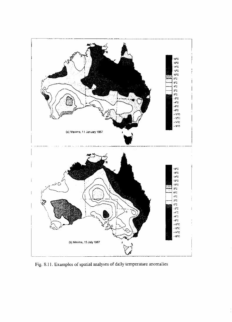
(a) Maxima, 11 January 1957
(b) Minima, 15 July 1987
Fig. 8.11. Examples of spatial analyses of daily temperature anomalies
1a•c 18°C
14"C
12"C
10"C
a•c a•c 4°C
2"C
o•c -2"C
-4"C
-6"C
-a•c -10"C
-12"C
-14"C
-16"C
1B"C
16"C
14"C
12"C
1o•c a•c s•c 4"C
2"C
o•c -2"C
-4·c -s•c -a·c -10"C
-12"C
-14"C
-16"C
8.6. Summary
The spatial averages calculated in this section reinforce the results obtained from
individual stations in Chapter 7. They show a tendency towards an increase in the
frequency of warm extremes and a decrease in the frequency of cool extremes, with
particularly marked trends noticeable for low minimum temperatures in Queensland. The
relationship of Queensland minimum temperatures to the El Nino-Southern Oscillation,
which has itself shown a trend towards more frequent El Nino conditions, will be
investigated further in Chapter 9.
193

Chapter9
Relationships between the Southern Oscillation Index (SOl)
and the frequency of extreme temperatures in Australia
9.1. Introduction
The relationship between the El Nino-Southern Oscillation (ENSO) and Australian
rainfall has received considerable attention (e.g. Quayle, 1929; Pittock, 1975;
McBride and Nicholls, 1983). There has been more limited attention given to the
relationship between ENSO and Australian temperatures, especially at the seasonal
(as opposed to annual) timescale.
The simultaneous relationship between ENSO and the mean seasonal maximum and
minimum temperature over Australia has been most thoroughly examined by Jones
(1999) and Jones and Trewin (2000a). Their major findings, in general, were that
significant simultaneous con·elations existed:
Sununer nzewz maximum temperature
Strong negative correlations (up to -0.6) were found in much of northern and eastern
Australia, whilst strong positive correlations were found locally in southern Victoria,
Tasmania and the central west coast of Western Australia.
Winter nzewz nuL\:inwm temperature
Strong negative correlations (typically -0.3 to -0.5) were found over most of
Australia south of the tropics, whilst positive correlations were found in the north,
strongest over Cape York Peninsula and in the Top End of the Northern TetTitory.
195
Summer mean minimum temperature
The pattern of positive and negative correlations was similar to that for maximum
temperatures, but the negative correlations were weaker, except in north-western
Australia.
Winter mean minimum temperature
Positive correlations were found over much of the eastern two-thirds of Australia, but
were significant only over New South Wales and the far north. Negative correlations
were found through much of southern Western Australia in winter and spring,
reaching up to -0.5 in the south-west in spring.
Lough (1995, 1997) examined the relationship between an areally-averaged
temperature series for Queensland and the SOl over the summer (October-March) and
winter (April-September) half-years. Her conclusions agreed broadly with those
above. She also found substantial interdecadal variability in the SOl-temperature
relationship, with the relationship between summer temperature (maximum and
minimum) and the SOl almost disappearing in the 1931-50 period, but that for winter
minimum temperature reaching its greatest strength during that period. This will be
discussed further later in this chapter.
The only Australian study to make ex tcnsi ve consideration of extreme temperatures
(as opposed to means) was that of Stone et a!. ( 1996). Using thresholds ranging
between -3°C and 3°C to define 'frost' at a number of stations in interior eastern
Queensland and northern New South Wales, they examined the relationship between
the May SOl and the total number of frosts for the following season. For most
thresholds, they found negative coiTelations (generally in the -0.25 to -0.4 range)
which were significant at the 5% level for most of the Queensland sites, but only
weak (and non-significant) con·elations, generally negative, for the no1ihem New
South Wales sites. Outside Australia, Gershunov and Barnett (1998) examined the
relative frequencies of temperatures above the 95th percentile and below the 5th
percentile in the United States winter during El Nifio and La Nifia conditions, finding

substantial differences between the two, particularly in the case of the frequencies of
extreme high temperatures.
9 .2. Methods of analysis
Two forms of analysis were carried out. These involved:
(a) The correlation between the SOl and the frequency of temperatures above given
temperature thresholds.
(b) The examination of the relative frequencies of days with temperatures above or
below certain thresholds in each of three categories of seasons, stratified by terci les of
the SOL
CoiTelations were caiTied out between the following data sets:
(a) The three-month mean SO I and the frequency of temperatures above the 5, 10, 15,
... , 90, 95 percentile levels for the sitnultaneous three-month period ('simultaneous
carrel ations ')
(b) The three-month n1ean SOl and the frequency of temperatures above the 5, 10, 15,
... , 90, 95 percentile levels for the following three-month period ('lag correlations')
In each case:
1. The correlations were calculated separately for maximum and minimum
temperature, using the full period of available record, and for each of the twelve
possible three-month periods (January-March through to December-February).
2. The daily maximum and minimum temperatures used were standardised
anomalies, as defined in Chapter 6.
3. The percentile thresholds used for each station were calculated using the
procedure in Chapter 8, with all available data used.
4. For each individual three-month period, the frequency of temperatures above each
percentile threshold was calculated as a percentage of all possible observations
during the period. The frequency was regarded as missing for a given three-month
period if there were fewer than 60 observations during that period.
197

5. The SOl used was based on the mean and standard deviation of Darwin-Tahiti
pressure anomaly differences between 1933 and 1992 (source: Bureau of
Meteorology web site, http://www .bom.gov .au/climate/current/soihtm 1.shtml)
In the case of the lag correlations, the results are attributed to the season whose
temperatures are under review (for example, the June-August (winter) results are for
the correlation between June-August threshold exceedances and March-May SOl).
Negative correlations indicate a tendency for more wann (fewer cold) days in El Nifio
years, whilst positive correlations indicate a tendency for fewer warm (more cold)
days in La Nifia years.
The bulk of the discussion of the results will concentrate on con·elations for the 1oth
and 90th percentiles. Correlations for the 501h percentile are also shown, in order to
indicate how ENSO affects the median (as opposed to the extremes).
In the comparison of relative frequencies of days with temperatures above or below
thresholds in the three SOl terciles:
1. Four types of events were examined: the frequency of days with temperatures
below the 10111 percentile, and above the 90 111 percentile, separately for maximum
and minimum tempenttures.
2. The SOl used was a three-month mean value. The terci le boundaries were
calculated using the full 1876-1999 SOI data set. The boundaries were calculated
separately for each of the twelve possible three-month periods, although only the
four calendar seasons, spring (September-November), summer (December
February), autumn (March-May) and winter (June-August), were examined in any
detail.
3. As for the correlations, the analysis was carried out for values of the SOl for the
season simultaneous with that for which the temperatures were being reviewed,
and for SOl values one season before the temperature measurements (lag
sensitivities).
192

4. Each day was sorted into one of three categories, depending on which tercile the
relevant three-month mean SOl fell into. The frequency of temperatures beyond
the overall thresholds above was then calculated for each tercile. (The terciles will
henceforth be referred to as terciles 1, 2 and 3, with 1 denoting the lowest one
third of SOl values and 3 the highest one-third).
5. A.s a measure of the sensitivity of the frequency of extreme temperatures to the
SOl, the following ratio was calculated for all thresholds, and both simultaneously
and at lag:
(Frequency of temperature beyond threshold in SOl tercile 1)
(Frequency of temperature beyond threshold in SOl tercile 3)
Ratios substantially above 1 indicate a tendency to more extreme events in El
Nifio years, whilst ratios substantially below 1 indicate a tendency to more
extreme events in La Nina years.
6. The standardised temperature anomalies, percentile thresholds and SOl definitions
were as for the analysis of con·elations above.
9.3. l{elationships between extreme temperature fre<Juency and the S()l
Figs. 9.1 a-1 show the correlations r between the frequencies of maximum and
rninimum temperatures above the 90, 50 and 10 percentile levels and the SOl, both
simultaneously and at one season's lag. The maps are drawn by using a four-pass
Barnes analysis (see Chapters 4 and 8) on data from each of the 103 stations. The time
series from the stations vary in length from 22 to 142 years.
Figs. 9.2a-h show the ratio between the frequency of extreme events in SOl tercile 1
and the frequency in tercile 3, as defined in section 9.2 above. A full listing of the
correlations and ratios for each station is given in Tables F. I and F.2.
199
I
_j

9.3.1. High maximum temperatures
F. 9 1 d 9 lb show the simultaneous and lag correlations between the SC)I and 1gs. . a an . th '1 the frequency of maxima above the 90 percent! e.
In spring, strong negative correlations exist, both simultaneously and at lag. in tW<l
distinct areas; the south-west of Western Australia and south-eastern Australia,
comprising most of Victoria, Tasmania, and New South Wales west of the Great
Dividing Range. They are below -0.4 in much of Victoria and inland southern New
South Wales, and reach -0.5 locally in Western Australia. Positive con·elaticms exist
over most of tropical Australia simultaneously (with the boundary moving further
north at lag). Values exceed 0.3 in parts of the far north simultancously1 hut only
locally at lag.
Negative correlations dominate mainland Australia in summer, with the strongest
correlations being in Queensland and New South Wales. The simultaneous and lag
patterns are very similar, with values below -0.3 over almost all or Queensland.
except for parts of the coast, and much of New South Wales. Much of this area hus
values below -0.4, and -0.6 is reached locally in inland northern Queensland. Positive
correlations are confined to Tasmania and the coastal fri ngcs of Victoria, South
Australia, and Western Australia south of Learmonth, and only at C'arnarvon and
Robe (both sites highly exposed to the ocean that arc somewhat unrepresentative of
their wider regions, as reflected by very strong gradients of mean summer rnaxin1un1
temperature (Bureau of Meteorology, 1998b )) do they reach 0.3.
As in summer, negative conelations dominate mainland Australia in auturnn. 'The
simultaneous conelations are mostly weak, with only a few stations below -0.3.
However, at lag there are strong correlations through much of tropical Australia, with
values below -0.3 over most of that area, reaching -0.5 in central Queensland.
The simultaneous winter correlations show a striking north-south divide. Strong
positive correlations (exceeding 0.4) are evident over tropical Queensland and the
Northern Territory, with values as high as 0.6 over Cape York Peninsula. In contrastt
negative correlations below -0.3 occur over most of Australia south of 28°S, except
200

Spring
Autumn t
-.
~ t:Jt
1.0
0.5
0.4
0.3
0.2
0.0
-0.2
-0.3
-0.4
-0.5
- -1.0
1.0
0.5
0.4
0.3
0.2 0.0
-0.2
-0.3
-0.4
-0.5
-1.0
1.0
0.5
0.4
0.3
0.2
0.0
-0.2
-0.3
-0.4
-0.5
- -1.0 6
t) Summer
"
~ 1.0
0.5
0.4
0.3
0.2 0.0
-0.2
-o.3
-0.4
-0.5
-1.0 \
Fig. 9.1 a. Correlation between frequency of maxima above the 90th percentile and SOl, simultaneous
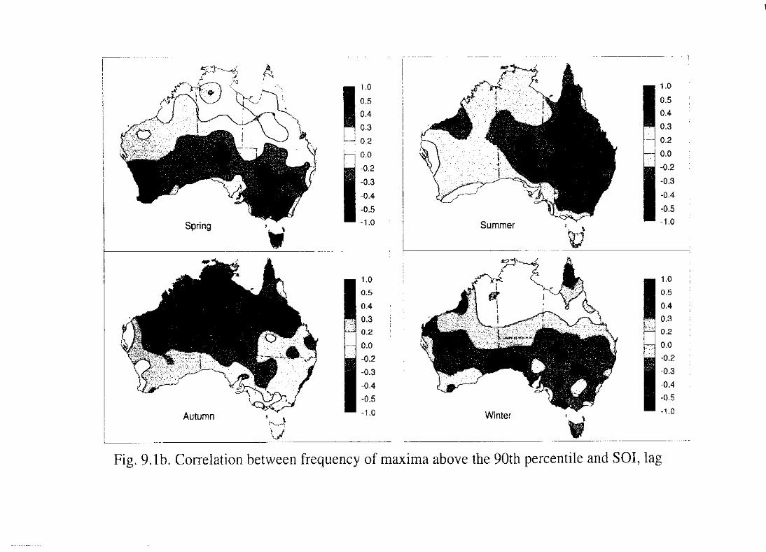
Spring
Autumn
A l
e ~ vJ
1.0
0.5
0.4
0.3
0.2
0.0
-0.2
-0.3
-0.4
-0.5 -1.0
1.0
0.5
0.4 0.3 0.2
0.0 -0.2
-0.3
-0.4
-0.5
-1.0
Summer 'tj
\
1.0
0.5 0.4 0.3
0.2
0.0
-0.2
-0.3
-0.4
-0.5 -1.0
1.0
0.5
0.4 0.3 0.2
0.0 -0.2
-0.3
-0.4 -0.5
-1.0
Fig. 9.lb. Correlation between frequency of maxima above the 90th percentile and SOl, lag

-- .-~----~
1.0 1.0
0.5 0.5 0.4 0.4
0.3 0.3
0.2 0.2
0.0 0.0
-0.2 -0.2
-0.3 -0.3
-0.4 -0.4
-0.5 -0.5
Spring c ~ .. - -1·0 Summer -1.0
1.0 1.0 0.5 0.5
0.4 0.4 0.3 0.3 0.2 0.2
0.0 0.0 -Q.2 -0.2
-Q.3 -0.3
-Q.4 -0.4
-o.s -0.5
Autumn ' - -1.0 e -1.0
\!} '- \ '
Fig. 9.1c. Correlation between frequency of maxima above the 50th percentile and SOl, simultaneous
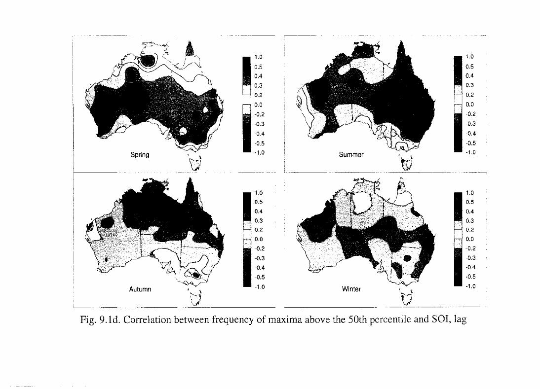
1.0 1.0
0.5 0.5
0.4 0.4
0.3 0.3
0.2 0.2
0.0 0.0
-0.2 -0.2
-0.3 -0.3
-0.4 -0.4
-0.5 -0.5
Spring ... - -1.0 Summer c -1.0
1.0 1.0 0.5 0.5
0.4 0.4
0.3 0.3 0.2 0.2
0.0 0.0 -().2 -0.2
-0.3 -o.3
-().4 -0.4
-0.5 -0.5
Autumn ' - -1.0 -1.0
M t~·
Fig. 9.ld. Correlation between frequency of maxima above the 50th percentile and SOl, lag

Spring T
~ \
\1 '
~
Autumn ' \ N tJ
i .0
0.5
0.4
0.3
0.2
0.0
-0.2
-0.3
-0.4
-0.5 - -1.0 I Summer
i.O
0.5
0.4 0.3 0.2
0.0
-0.2
-0.3
-0.4
-o.5
- -1.0 \
1.0
0.5 0.4
0.3
0.2
0.0
-0.2
-0.3
-0.4
-0.5 -1.0
1.0
0.5
0.4
0.3 0.2
0.0
-0.2
-0.3
-0.4
-0.5
-1.0
Fig. 9.1 e. Correlation between frequency of maxima above the 1Oth percentile and SOl, simultaneous

1.0
0.5
0.4
0.3
0.2
0.0
-0.2
-0.3
-0.4
-0.5
Spring ... - -1.0 I Summer " \
~ ~
1.0
0.5
0.4
0.3 0.2
0.0
-o.2 -0.3
-0.4
-0.5
B Autumn D - -1.0
~~ -~J.j
Fig. 9.1f. Correlation between frequency of maxima above the lOth percentile and SOl, lag
1.0
0.5 0.4
0.3
0.2
0.0
-0.2
-0.3
-0.4
-0.5 -1.0
1.0
0.5
0.4
0.3 0.2
0.0
-0.2
-0.3
-0.4
-0.5
-1.0

Spring -.
s v
Autumn ' \
M v
1.0
0.5
0.4
0.3 0.2
0.0
-0.2
-0.3
-0.4
-0.5 - -1.0
1.0 0.5
0.4
0.3 0.2
0.0
-Q.2
-Q.3
-0.4
-0.5
- -1.0
I Summer
D
~1 ttl
1.0
0.5
0.4
0.3
0.2
0.0
-0.2
-0.3
-0.4
-0.5 -1.0
1.0 0.5
0.4
0.3 0.2
0.0
-0.2
-o.3 -0.4
-0.5
-1.0
Fig. 9.lg. Correlation between frequency of minima above the 90th percentile and SOl, simultaneous
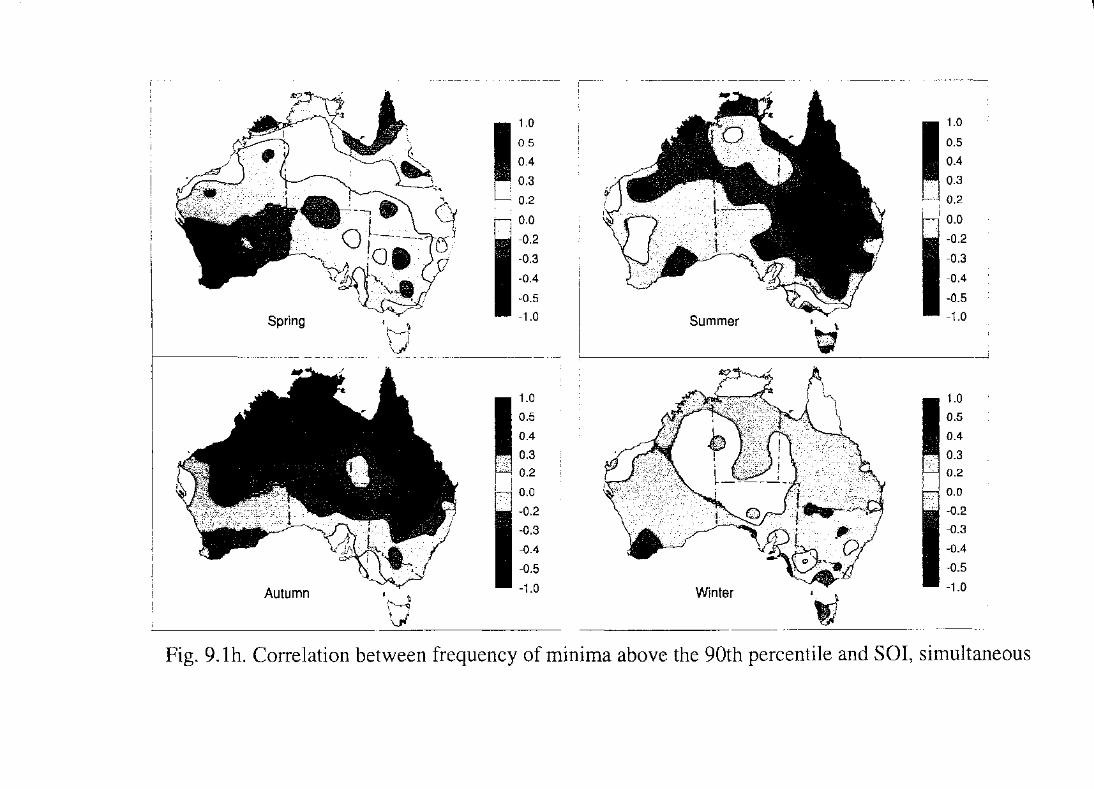
Spring ~
H v ~
Autumn &
~ \ I
\yl
1.0
0.5
0.4
0.3 0.2
0.0
-0.2
-0.3
-0.4
-0.5 - -1.0
1.0 0.5
0.4
0.3 0.2
0.0
-0.2
-o.3 -0.4
-0.5
- -1.0
I Summer
\
1.0
0.5
0.4
0.3
0.0
-0.2
-0.3
-0.4
-0.5 -1.0
1.0 0.5
0.4 0.3 0.2
0.0
-0.2 -0.3
-0.4
-0.5
-1.0
Fig. 9.1h. Correlation between frequency of minima above the 90th percentile and SOl, simultaneous
,

Spring ..
' ..
Autumn I
H ~
1.0
0.5
0.4
0.3 0.2
0.0
-0.2
-0.3
-0.4
-0.5
- -1.0
1.0 0.5
0.4
0.3
0.0
-Q.2
-0.3
-0.4
-0.5
-1.0
Summer
'tr~ ·J
1.0
0.5
0.4
0.3 0.2
0.0
-0.2
-0.3
-0.4
-0.5 -1.0
1.0 0.5
0.4
0.3 0.2
0.0
-0.2 -0.3
-0.4
-0.5
-1.0
Fig. 9.1i. Correlation between frequency of minima above the 50th percentile and SOl, simultaneous
1

kit'~~ _.,.~-r ,.1
·- j;.. ~t} 1.0 1.0
0.5 0.5
0.4 0.4
0.3 0.3 0.2 0.2
0.0 0.0
-0.2 -0.2
-0.3 -0.3
-0.4 -0.4
-0.5 -0.5
Spring : .. - -1·0 Summer -1.0
Autumn ;
N ~ ~ \.Jfl
1.0 0.5
0.4
0.3 0.2
0.0
-0.2
-0.3 -0.4
-0.5
-1.0
'ti Fig. 9.lj. Correlation between frequency of minima above the 50th percentile and SOl, lag
1.0
0.5
0.4
0.3 0.2
0.0
-0.2 -0.3 -0.4
-0.5
-1.0

1.0 1.0
0.5 0.5
0.4 0.4
0.3 0.3
0.2
0.0 I !
-0.2 I
-0.3 I I
-0.4 j
~ fJ' I
I
Spring
-0.5 !
·\,~. ·""~·~' L
.. i
"-(-" ' . \.. ·'
:
~\~·e.
H - -1.0 !
-0.4
I ~'
v I
Summer
-0.5
I l
' H -1.0
v
1.0 1.0 0.5 0.5 0.4 0.4 0.3 0.3 0.2 0.2
0.0
-0.2
-0.3 -0.3
-0.4 -0.4
-0.5 -0.5
Autumn a
~ - -1.0
-v~
Winter i ~
~ -1.0
~ J v
Fig. 9.lk. Correlation between frequency of minima above the lOth percentile and SOl, simultaneous

, \
1.0 1.0
0.5 0.5
0.4 0.4
0.3 0.3
0.2 0.2
0.0 0.0
-0.2 -0.2
-0.3 -0.3
-0.4 -0.4
-0.5 -0.5
Spring -. - -1.0 Summer -1.0 g
tJ ' ti l
1.0 i 1.0 0.5 I 0.5
' 0.4 0.4 ' ' 0.3 I 0.3
0.2 0.2
0.0 0.0
-0.2 -0.2
-0.3 -0.3
-0.4 -0.4
-0.5 -0.5
Autumn D - -1.0
B -1.0
~~ Vi ~1
Fig. 9.11. Correlation between frequency of minima above the 1Oth percentile and SOl, lag

Spring
Autumn I
~ \If
10.0 3.0 2.0 1.8 1.5 1.3 1.2 1.1 1.0 0.9 0.8 0.7 0.6 0.5 0.4 0.0
10.0 3.0 2.0 1.8 1.5 1.3 1.2 1.1 1.0 0.9 0.8 0.7 0.6 0.5 0.4 0.0
Summer
\
10.0 3.0 2.0 1.8 1.5 1.3 1.2 1.1 1.0 0.9 0.8 0.7 0.6 0.5 0.4 0.0
10.0 3.0 2.0 1.8 1.5 1.3 1.2 1.1 1.0 0.9 0.8 0.7 0.6 0.5 0.4 0.0
Fig. 9.2a. SOl tercile 1/tercile 3 event frequency ratio, maxima above 90th percentile, simultaneous
1

Spring
Autumn ~
- -·-· ··-- --------·------·--
10.0 3.0 2.0 1.8 1.5 1.3 1.2 1.1 1.0 0.9 0.8 0.7 0.6 0.5 0.4 0.0
10.0 3.0 2.0 1.8 1.5 1.3 1.2 1.1 1.0 0.9 0.8 0.7 0.6 0.5 0.4 0.0
Summer
Winter ~
Fig. 9.2b. SOl tercile 1/tercile 3 event frequency ratio, maxima above 90th percentile, lag
10.0 3.0 2.0 1.8 1.5 1.3 1.2 1.1 1.0 0.9 0.8 0.7 0.6 0.5 0.4 0.0
10.0 3.0 2.0 1.8 1.5 1.3 1.2 1.1 1.0 0.9 0.8 0.7 0.6 0.5 0.4 0.0
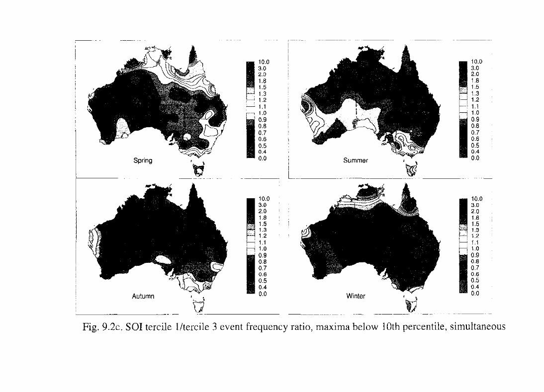
Spring
Autumn
·~.)L';···;:'i \]!
10.0 3.0 2.0 1.8 1.5 1.3 1.2 1.1 1.0 0.9 0.8 0.7 0.6 0.5 0.4 0.0
10.0 3.0 2.0 1.8 1.5 1.3 1.2 1.1 1.0 0.9 0.8 0.7 0.6 0.5 0.4 0.0
Summer
\
10.0 3.0 2.0 1.8 1.5 1.3 1.2 1.1 1.0 0.9 0.8 0.7 0.6 0.5 0.4 0.0
10.0 3.0 2.0 1.8 1.5 1.3 1.2 1.1 1.0 0.9 0.8 0.7 0.6 0.5 0.4 0.0
Fig. 9.2c. SOl tercile 1/tercile 3 event frequency ratio, maxima below lOth percentile, simultaneous

Spring
Autumn
~~ f;:;;i
10.0 3.0 2.0 1.8 1.5 1.3 1.2 1.1 1.0 0.9 0.8 0.7 0.6 0.5 0.4 0.0
10.0 3.0 2.0 1.8 1.5 1.3 1.2 1.1 1.0 0.9 0.8 0.7 0.6 0.5 0.4 0.0
Summer
\
Fig. 9.2d. SOl tercile 1/tercile 3 event frequency ratio, maxima below 1Oth percentile, lag
10.0 3.0 2.0 1.8 1.5 1.3 1.2 1.1 1.0 0.9 0.8 0.7 0.6 0.5 0.4 0.0
10.0 3.0 2.0 1.8 1.5 1.3 1.2 1.1 1.0 0.9 0.8 0.7 0.6 0.5 0.4 0.0
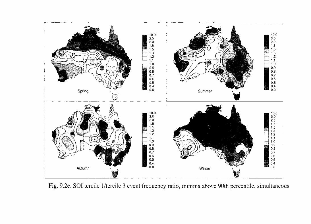
Spring
Autumn \
10.0 3.0 2.0 1.8 1.5 1.3 1.2 1 .1 1.0 0.9 0.8 0.7 0.6 0.5 0.4 0.0
10.0 3.0 2.0 1.8 1.5 1.3 1.2 1.1 1.0 0.9 0.8 0.7 0.6 0.5 0.4 0.0
Summer
Winter \
10.0 3.0 2.0 1.8 1.5 1.3 1.2 1.1 1.0 0.9 0.8 0.7 0.6 0.5 0.4 0.0
10.0 3.0 2.0 1.8 1.5 1.3 1.2 1.1 1.0 0.9 0.8 0.7 0.6 0.5 0.4 0.0
Fig. 9 .2e. SOl tercile 1/tercile 3 event frequency ratio, minima above 90th percentile, simultaneous
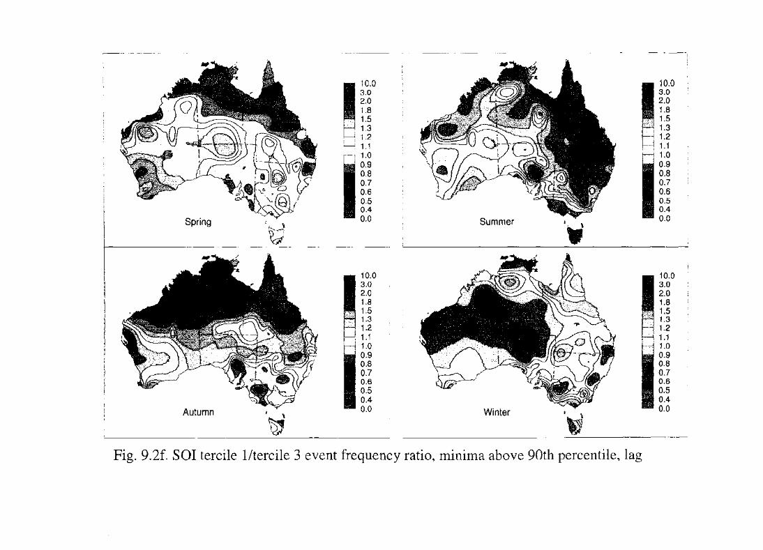
10.0 3.0 2.0 1.8 1.5 1.3 1.2 1.1 1.0 0.9 0.8 0.7 0.6 0.5 0.4
Summer -0.0 I -. Spring 't;J ~
10.0 3.0 2.0 1.8 1.5 1.3 1.2 1.1 1.0 0.9 0.8 0.7 0.6 0.5 0.4
-0.0 T
' ~
Autumn
'
\
Fig. 9.2f. SOl tercile 1/tercile 3 event frequency ratio, minima above 90th percentile, lag
10.0 3.0 2.0 1.8 1.5 1.3 1.2 1.1 1.0 0.9 0.8 0.7 0.6 0.5 0.4 0.0
10.0 3.0 2.0 1.8 1.5 1.3 1.2 1.1 1.0 0.9 0.8 0.7 0.6 0.5 0.4 0.0

10.0 10.0 3.0 3.0 2.0 2.0 1.8 1.8 1.5 1.5 1.3 1.3 1.2 1.2 1.1 ' 1.1 1.0 ' 1.0 0.9 0.9 0.8 0.8 0.7 0.7 0.6 0.6 0.5 0.5 0.4 0.4
Spring "T -0.0 Summer 0.0 f
ti B
'd 10.0 10.0 3.0 3.0 2.0 2.0 1.8 1.8 1.5 1.5 1.3 1.3 1.2 1.2 1.1 I 1.1 1.0 1.0 0.9 0.9 0.8 0.8 0.7 0.7 0.6 0.6 0.5 0.5 0.4 0.4
Autumn -. -0.0 0.0 1
\9 •
~ Fig. 9.2g. SOl tercile 1/tercile 3 event frequency ratio, minima below lOth percentile, simultaneous
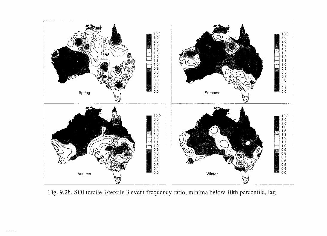
Spring
Autumn I
~
10.0 3.0 2.0 1.8 1.5 1.3 1.2 1.1 1.0 0.9 0.8 0.7 0.6 0.5 0.4 0.0
10.0 3.0 2.0 1.8 1.5 1.3 1.2 1.1 1.0 0.9 0.8 0.7 0.6 0.5 0.4 0.0
Summer
I
~ \d
Fig. 9.2h. SOl tercile 1/tercile 3 event frequency ratio, minima below 1Oth percentile, lag
10.0 3.0 2.0 1.8 1.5 1.3 1.2 1.1 1.0 0.9 0.8 0.7 0.6 0.5 0.4 0.0
10.0 3.0 2.0 1.8 1.5 1.3 1.2 1.1 1.0 0.9 0.8 0.7 0.6 0.5 0.4 0.0

for New South Wales east of the Great Dividing Range and far eastern Gippsland,
with values locally reaching -0.5 in several places. At lag, the positive/negative
pattern is similar to that for the simultaneous con-elations, but the con-elations
themselves are much weaker, although -0.3 is still reached at scattered locations
through southern Australia and 0.4 on Cape York Peninsula.
Figs. 9.2a and 9.2b show the relative sensitivities of the frequency of extreme high
maxima to the SOL As expected, the geographical patterns of the ratios largely mirror
the correlations discussed above. The simultaneous winter pattern is particularly
striking. The ratio is below 0.5 over most of the region north of 20°S, and above 2.0
in much of south-western Western Australia and inland New South Wales. These
indicate shifts in probabilities of extreme high maxima exceeding 2:1 (in either
direction) between El Nifio and La Nifia conditions. However, as for the winter
con·elations, these relationships are much weaker at lag.
Other regions and seasons where the ratios are above 1.5 are:
• Much of Tasmania, Victoria, inland New South Wales and south-western Western
Australia in spring, both simultaneously and at lag.
• Most of Queensland (apart from the tropical coast) and New South Wales in
summer, with greater sensitivities (widely exceeding 2.0 in Queensland, and
reaching 3.0 in places) at lag than simultaneously.
• Most of tropical Australia at lag in autumn, with sensitivities exceeding 2.0 in
most of north-western Australia. Such ratios are also observed more locally
simultaneously in not1hern Western Australia and the western Northern TeiTitory.
Ratios below 0.7 are less common. Apart from the aforementioned very low values in
the tropics during winter, low simultaneous ratios (mostly 0.5-0.7) occur in spring
over the region north of l8°S, but those ratios are somewhat higher at lag. These
results suggest that, over Australia as a whole, extreme high temperature events are
most likely during El Nifio events.
201

9.3.2. Low maximum temperatures
Figs. 9.1e and 9.1f show the simultaneous and lag correlations between the SOl and
the frequency of maxima above the lOth percentile. In spring, simultaneous and lag
correlations are negative over most of Australia, except for parts of northern
Australia, southern Victoria and parts of Tasmania. However, the correlations only
reach -0.3 in small isolated areas, mostly in Western Australia. The correlations are
slightly stronger at lag than they are simultaneously, with values locally reaching -0.5
at Halls Creek and isolated Queensland stations also reaching -0.3. Isolated stations
on the northern coastline have correlations exceeding 0.3.
As for high maxima, negative correlations dominate most of Australia in summer,
although the focus of the strongest correlations is further north and west.
Simultaneous correlations are below -0.3 over almost all of Queensland, the Northern
Territory and tropical Western Australia, reaching -0.6 in the far north. At lag the
correlations are slightly weaker but are still below -0.3 over much of Queensland and
the Northern Territory. Positive correlations are mostly confined to the south-east,
covering Tasmania (where they reach 0.3 locally), most of Victoria and adjoining
parts of New South Wales and South Australia. The area of positive correlations in the
south-east is more extensive for low maxima than it is for high n1axima, and it is
interesting to note that some stations ncar the NSW/Victorian border show positive
correlations ncar 0.3 for low maxima, hut negative correlations ncar -0.3 for high
maxima, indicating enhanced (suppressed) variability of temperature at holh ends of
the distribution in El Nifio (La Nina) years. This may be associated with positive
pressure anomalies over the South Tasman Sea, and consequent north-easterly
gradient wind anomalies over south-eastern Australia, in La Nina years (Drosdowsky
and Wi !Iiams, 1991; 1 ones and Simmonds, 1994 ).
In autumn, negative simultaneous coiTelations are observed over most of Australia.
They are mostly weak, with -0.3 reached only in the northern half of Queensland,
parts of the Northern Territory and the Kimberley region of Westetn Australia. In
contrast to the situation for high maxima, the correlations are even weaker at lag, and
(mostly weak) positive correlations cover substantial parts of the continent, 0.3 being
reached locally in Victoria.
202

"'inter correlations are negative over almost all of Australia except the far north, both
simultaneously and at lag. Unlike the other extreme variables in winter, the
correlations at lag are of similar or greater strength to those found simultaneously,
except that the strong positive correlations found simultaneously in the far north
(locally exceeding 0.5 on Cape York Peninsula) disappear at lag. Simultaneous values
below -0.3 are found at scattered locations through inland eastern Australia, whilst at
lag they are found over much of Queensland (except for Cape York), reaching -0.5
near Brisbane.
Figs. 9.2c and 9.2d show the relative sensitivities of the frequency of extreme low
rnaxima to the SOL The relative sensitivity of the frequency of low maxilna to the
SOl is, on balance, generally greater than those found for similar cotTelations for high
n1axima. Ratios below 0.7 are found in the following areas:
• Widespread areas in a belt across the central latitudes of Australia in spring.
• Most of Queensland, the Northern Territory and northern Western Australia in
summer. The areas are more extensive, and stronger, at lag than they are
simultaneously, extending southwards into northern New South Wales are with
values below 0.5 in the Top End of the Northern Territory.
• Most of Western Australia (except for the west and south coasts), the Northern
Ten·itory, Queensland and northern South Australia for si1nultaneous values in
autumn, with ratios as low as 0.4 in the northern Northern TetTitory. As with the
correlations, the pattern weakens considerably at lag, with values below 0.7
mostly confined to the region north of 20°S.
• Large areas of central and eastern Australia in winter (reaching 0.5 in inland
southern Queensland). Unlike the correlations, the pattern for ratios is somewhat
weaker at lag than it is simultaneously (at lag ratios below 0.7 are mostly confined
to Queensland and northern New South Wales), but the weakening of the
relationship is still much less distinct than it is for the other three extremes.
Simultaneous ratios above 1.5 are only found at isolated stations, mostly in the far
north in winter and spring. At lag, the one season where coherent areas with ratios
203

above 1.5 occur is autumn, where they are found over much of Victoria and adjacent
southern inland New South Wales, parts of Tasmania, and the Pilbara and Gascoyne
regions of Western Australia.
9.3.3. High minimum temperatures
Figs. 9.lg and 9.1h show the simultaneous and lag con·elations between the SOI and
the frequency of minima above the 90th percentile. In spring, correlations are positive
in most of tropical Australia, both simultaneously and at lag. Simultaneous values
above 0.3 occur over most of the area north of a line from Brisbane to the Kimberley,
reaching as high as 0. 7 on Cape York Peninsula. The posi ti ve/negati ve boundary is in
a similar location at lag but the positive correlations are weaker, only reaching 0.3 in
the far north. Negative correlations between -0.3 and -0.5 occur in south-western
Western Australia, with near-zero con-elations over most of the remaining
extratropics.
Negative correlations occur over most of Australia in summer. They are stronger at
lag than simultaneously, with values below -0.3 covering most of Queensland and
inland New South Wales. Positive correlations, both simultaneously and at lag, occur
in Victoria, Tasmania and the south-cast of South Australia, exceeding 0.3 at some
mainland coastal stations and in much of Tasmania.
Simultaneous correlations in autumn arc weak throughout Australia, although positive
correlations cover the south-cast south of 30°S, with values reaching 0.3 at a few
stations. At lag, however, negative correlations cover almost all of mainland
Australia, and are below -0.3 over almost all of the tropics and extratropica]
Queensland (reaching -0.6 in central Queensland). Interestingly, the change between
the simultaneous and lag patterns is the reverse of that which occurs for low maxima.
In winter, positive correlations occur over most of Australia, except for southern
Western Australia and the coasts of Victoria and South Australia, and exceed 0.3 over
extensive areas of the tropics. However, these correlations disappear almost
completely at lag, with values between 0.2 and -0.2 at almost all stations.
Figs. 9.2e and 9.2f show the relative sensitivities of the frequency of extreme high
minima to the SOl. Notable features include:
• The very low ratios found simultaneously in winter and spring in the far north of
Australia. Ratios are below 0.5 in both seasons at numerous stations, are below 0.7
over most of the tropics, and fall as low as 0.2 on Cape York Peninsula. These low
ratios are also found at lag in spring, but not in winter.
• There are extensive areas with ratios at lag exceeding 1.5 in both summer and
autumn. In summer those ratios occur over most of Queensland, northern and
central New South Wales and some northern coastal areas of the Northern
Territory and Westen1 Australia. In autumn they cover the entire tropics. In both
cases the ratios exceed 2.0 over substantial regions and 3.0 at a few stations. These
patterns are also found simultaneously in summer, but not in autumn.
• Ratios drop below 0.7 in summer, both simultaneously and at lag, in summer in
southern Victoria and Tasmania. Conversely, in winter this is the only portion of
the country with ratios approaching 1.5.
• Simultaneous ratios exceed 1.5 in spring in south-western Western Australia, and
are still well above 1 (although mostly dropping to 1.3-1.4) at lag.
9.3.4. Low minimum temperatures
Figs. 9.1 k and 9.11 show the sitnultaneous and lag correlations between the SOl and
the frequency of minima above the lOth percentile. In spring, the only areas with
strong correlations (lrl > 0.3) are patis of inland southern and central Westct·n
Australia, where correlations are between -0.3 and -0.5, and two small areas where
positive con·elations exceed 0.3: Cape York Peninsula and an area on either side of
the NSW/Victoria border. The simultaneous and lag patterns are similar.
Weak simultaneous correlations are also a feature of summer. Whilst negative
con·elations are widespread in Western Australia, they only reach -0.3 at a few widely
scattered stations. Positive correlations are found in much of south-eastern Australia
but only reach 0.3 at some exposed coastal stations in Victoria and Tasmania. At lag,
the pattern is somewhat different with negative correlations over most of Australia
205

except for Victoria and Tasmania, but values are still generally above -0.3, with that
threshold being reached in several areas in northern Western Australia, the Northern
Territory and inland southern Queensland.
In autumn there is a marked contrast between the simultaneous and lag patterns. The
simultaneous correlations are weakly positive over most of the country except for the
western half of Western Australia, and exceed 0.3 over parts of Victoria, southern
New South Wales and northern Queensland. At lag, however, values are negative over
most of the mainland, and are near or below -0.3 over much of the tropics. Over New
South Wales and northern Victoria, the frequency of minima below the lOth percentile
in years with a summer SOl in tercile 2 is generally somewhat above the frequency in
years when it is in either tercile 1 or 3, one of the few examples of a substantial
anomaly being associated with near-neutral SOl conditions.
Positive simultaneous correlations occur in winter over most of Australia, other than
the southetn two-thirds of Western Australia. They exceed 0.3 over a broad belt
stretching from Victoria to the Northern Tenitory, reaching 0.5 in northern Victoria
and southern New South Wales. These positive correlations, however, disappear
almost completely at lag, with most of the continent instead being dominated by weak
negative conelations, and stronger correlations ( -0.3 to -0.5) being found in the
northern half of Queensland, particularly ncar the Gulf or Carpentaria.
In general, the correlations for low minima, particularly at lag, arc weaker (in both
directions) than those found for the other three cxtrernc ten1perature parameters.
Figs. 9.2g and 9.2h show the relative sensitivities of the frequency of extreme low
maxima to the SOL The most striking feature of these is the high ratios observed
simultaneously through most of the eastern two-thirds of Australia in winter- and the
almost complete absence of high ratios over this area at lag. Simultaneously,
extensive areas have ratios exceeding 1.5, with values as high as 2.5 in southetn New
South Wales; at lag, only isolated stations even exceed 1.3. These results mirror those
for the correlations described above.
Ratios below 0.7 are found at lag through substantial parts of northern Australia in all
seasons except spring. For simultaneous ratios, though, such values are only found in
this region in summer, when they extend to an area centred on the NSW/Queensland
border. Ratios between 0.5 and 0.7 are also found over much of the southern half of
Western Australia in spring.
The results for ratios of low minima show less spatial coherence than for the other
three parameters. Some of this lack of coherence is the result of individual anomalous
seasons (e.g. Camooweal in summer 1994/95) which may be indicative of undetected
data quality problems. Low minimum temperatures are, however, generally more
dependent on local factors such as topography and site condition (Bootsma, 1976;
Kalma et al., 1986, 1992; see also section 3.2) than other extremes, and it might be
expected that this would contribute to a reduced spatial coherence of the patterns
shown in Figs. 9.2g and 9.2h.
9.4. Discussion and implications
Many of the results found for extreme temperatures are consistent with those
previously found for mean temperatures and noted in section 9.1. In particular, the
negative correlation between summer temperatures (especially maxima) and the SOl
through much of northern and eastern Australia affects most of the frequency
distribution of temperature fairly unifmmly. This is also true of the negative
correlations between the SOl and maximum and minimum temperatures in southern
Western Australia in spring.
There are, however, a number of locations where there are substantial differences
between the influence of the SOl on different parts of the frequency distribution. A
particularly notable example of this occurs for maximum temperatures in Victoria,
particularly southern Victoria, in spring and summer. Two cases characteristic of this
are Laverton ( 144°44' E, 37°52' S) in spring (where most percentile points up to the
75th show weak positive simultaneous correlations, but there is a negative correlation
of -0.48 for the 901h and 95th percentiles), and Rutherglen (146°30' E, 36°06' S) in
summer (where there is a simultaneous correlation of 0.26 for the lOth percentile, but
-0.35 for the 90th). This suggests that, in Victoria, El Nifio (La Nifia) conditions are
207
associated with enhanced (suppressed) variability of maximum temperatures, at both
ends of the frequency distribution, in spring and summer. When viewed in a spatial
sense, it is perhaps not surprising that the area of negative correlations in spring and
summer extends further south for extreme high temperatures than it does for median
temperatures (Figs. 9.1c/d), as extreme high temperatures in Victoria are generally
associated with airstreams of northerly origin and the maximum temperatures in such
airstreams might be expected to be influenced by conditions in the source regions for
the air, further north.
Another region where such effects are noticeable is northern Australia in winter and,
to a lesser extent, in spting. I-Iere, it is La Nifia that is associated with enhanced
temperature variability, with increased frequencies of both extreme low maxima and
high maxima. Two examples of this occur at Halls Creek (where the simultaneous
SOl correlations in winter are -0.13 for the 1oth percentile and 0.43 for the 901h) and
Camooweal ( -0.25 and 0.45 respectively).
A striking result is the marked seasonal reversal of the maximum temperature/SOl
relationships in northern Australia between winter and summer. This is noticeable
throughout the frequency distribution, par1icularly in northern Queensland. A good
example is Paltnervillc, where the simultaneous SOl/temperature frequency
correlations arc between 0.44 and 0.64 for all percentiles in winter, increase to 0.48"
0.66 for the July-September period (not mapped), and arc still weakly positive in
spd ng (0.00-0.36 ), but fall to -0.43- -0.57 in Sllln mer and -0.57 - -0.63 for the
January-March quarter. The negative correlations in summer can be associated with
enhanced rainfall and cloud cover during the tropical wet season in La Nina years
(Drosdowsky and Williams, 1991 ), but an explanation for the positive conelations in
winter and spting is less obvious.
There are few instances of substantial anomalies being associated with near-neutral
(tercile 2) SOl values, the most extensive instance being for low minima in autumn,
which occur with increased frequency in New South Wales and northern Victoria in
years when the summer SOl is near neutral. In general, the observed frequencies of
extreme events, for all parameters, in tercile 2 are intermediate between those in
terciles 1 and 3, although there are some instances where an anomaly is confined to

one of the three terciles (for example, the negative correlation between the SOl and
the frequency of extreme high maxima in winter in south-eastern Australia reflects a
increased frequency of such events in El Nino years, with frequencies in tercile 2
being similar to those in tercile 3).
The results obtained in section 9.3 indicate that an SOl-based scheme has potentially
useful skill in the seasonal forecasting of extreme temperatures some pat1s and
seasons of Australia. This is particularly true of maximum temperatures (both high
and low). The weakest results are for low minimum temperatures, suggesting that a
scheme based on the SOl alone has limited potential for the forecasting of extreme
low temperatures. As extreme low temperatures, pat1icularly outside the regular frost
season, are of great importance for some types of agriculture, as illustrated by the
estimated agricultural losses of $200 million in a frost in Victmia in October 1998
(Bureau of Meteorology, 1998a) this is a somewhat disappointing result.
Possible future extensions of the analysis
There are a number of ways in which this analysis could be extended further at a later
date. Stone and Auliciems (1992) defined five phases of the SOl (consistently
positive/negative/ncar zero, rapidly rising, rapidly falling). It would be possible to use
these phases, rather than SOl terciles, as categories into which to stratify extreme
temperature occurrences. This is likely to have pat1icular potential for those seasons
and parameters for which there is a dramatic difference between the simultaneous and
lag pattetns, as occurs in autumn and winter for some variables.
Another possible extension would be to incorporate information of sea surface
temperatures in the Indian Ocean, as well as the tropical Pacific (for which the SOl is
used as a suiTogate), in the analysis. Two empirical orthogonal functions (EOFs),
corresponding approximately to sea surface temperatures in the two oceans, are used
in the Australian Bureau of Meteorology's cunent operational scheme for the seasonal
forecasting of Australian rainfall and mean temperature (Drosdowsky and Chambers,
1998; Jones, 1998). A possible drawback to repeating the analysis of extreme
temperature frequencies in different Pacific/Indian Ocean temperature categories is
that the number of categories could become rather large (using three terciles of the
209

two EOFs, for example, would result in nine categories), which in turn would result in
fairly small samples in each category when only 40 years of record are available from
most stations.
The 'autumn predictability barrier', and comparisons with previous studies
Except for low maxima, the correlations were generally substantially weaker (and
ratios closer to 1) at lag than they were simultaneously in winter, but not in the other
three seasons. This is consistent with the well-known 'autumn predictability ban·ier'
of the El Nino-Southern Oscillation phenomenon itself (e.g. Torrence and Webster,
1998)~ the SOl shows much less persistence from the Southern Hemisphere autumn
into winter than it does in any of the other seasons.
A particularly interesting result in winter is that there are, in general, weak negative
cotrelations between the autumn SOl and the frequency of minima above the 1 01h
percentile in winter in most of Queensland. At first glance, this appears to contradict
the findings of Stone et al. (1996), who found negative cotrelations (mostly around -
0.3) between the May SOl and the number of days with temperatures below specified
thresholds at a number of Queensland stations. There are, however, at least four
differences between the two studies:
(a) The analysis in this chapter uses the three-month mean SOl for the March-May
period, whereas Stone et al. use the single-month value for May. This difference
may be significant in light of the previously-noted tendency for rapid changes in
the SOl during that period.
(b) The analysis in this chapter mostly uses data from the 1957-96 period, whereas
most stations used by Stone et al. had data from the 1910-93 period. Changes in
the decadal-to-multidecadal timescale in the climate (Power et al., 1999a), and, in
particular, in the relationship between the SOl and various climatic variables in
Australia, possibly associated with the Interdecadal Pacific Oscillation (Power et
al., 1999b), are well-known to have taken place. In particular, Lough (1997) found
substantial changes in the correlation between the SOI and mean minimum
temperatures for Queensland in the April-September period between 1931-50
210
-

(0.63) and 1975-95 (0.22). It would not be surprising if this weakening of the SOl
minimum temperature relationship were also observed for extreme temperatures.
(c) As shown in Chapters 7 and 8, there has been a very strong downward trend in the
frequency of low minimum temperatures in Queensland over the 1957-96 period.
There has also been a tendency towards an increased frequency of low autumn
SOl values towards the end of this period. Six of the last 10 years of the record
had an autumn SOl in tercile 1 (including five in succession between 1991 and
1995), compared with 9 of the 30 years between 1957 and 1986. It is possible that
an SOl-temperature relationship here has been masked by the effects of general
climate change. (A consequence, if this is indeed the case, is that this suggests that
the observed downward trend in the frequency of low minimum temperatures
would have been even stronger were it not for the behaviour of the SOl over this
period).
(d) The data sets used by Stone et al. were not adjusted for inhomogeneities. Whilst
this is likely to affect conclusions about the trends in temperatures that they found,
it should have a limited impact on the SOl-temperature relationship, as any bias in
temperatures during a section of the record will affect observations during that
period under both high and low SOl conditions.
The possibility of decadal-to-interdecadal variability in the nature of the SOl-extreme
temperature relationship is a particularly intriguing one. The 40 years of record
available from most stations for this study is insufficient to cany out an assessment of
this, but it is an area of considerable potential for future study once more pre-1957
daily data are digitised over the coming years.
211

Chapter 10
Conclusion
The central conclusion of this thesis is that the frequency of extreme high
temperatures, both maxima and minima, in Australia has increased over the period
between 1957 and 1996, and that the frequency of extreme low temperatures has
decreased. These results hold across most seasons, and in most regions, and are valid
for all of the thresholds tested, both fixed and relative (percentile-based). The
strongest observed trends are, in general, the decreasing trends in the frequency of
extreme low minimum temperatures, and the weakest are the increasing trends in the
frequency of extreme high maximum temperatures. This suggests a decline in
temperature variability over Australia during the 1957-1996 period, supetimposed
upon a general warming trend of mean temperatures over that period.
The declining trend in the frequency of extreme low temperatures is especially
marked in Queensland, where the annual frequency of m.inima below the lOth
percentile fell by 47o/cJ between 1957 and 1996, with the decline reaching 50o/o in
winter. This is a dramatic change, being of comparable magnitude to those projected
for New South Wales (accompanying a much larger warming of mean temperatures
than that observed so far in Queensland) by 2050 by the CSIRO climate model
(Hennessy ct al., 1998).
It was found in Chapter 6 that the frequency distributions of Australian daily
max1mum and minimum temperatures were most effectively represented by a
compound Gaussian distribution, being a composite of two or three individual
Gaussian distributions. Using this distribution, it was found that the observed change
in temperature over the 1957-1996 period was reflecting an increase in the means of
both the cooler and warmer parts of the frequency distribution, suggesting that the
changes, over Australia as a whole, represent warming of all air masses in the
Australian region (both continental and maritime), rather than a general circulation
change (although the question of whether changes in circulation have been
responsible for anomalous changes at individual stations remains unaddressed).
213

In Chapter 9, numerous relationships were found between the frequency of extreme
temperatures and the Southern Oscillation Index. These relationships were
particularly strong for extreme high maximum temperatures. With the exception of
the relationship of autumn SOl with winter temperatures, many of these relationships
remained robust at one season's lag. This suggests that there is considerable potential
for the seasonal forecasting of extreme temperature probabilities, especially if the
simple SOl-based scheme suggested by the work in Chapter 9 is refined to a more
sophisticated system, based on principal components of Pacific and Indian Ocean
temperatures, as is currently used by the Australian Bureau of Meteorology for
seasonal forecasting of mean temperatures and total rainfall. The seasonal forecasting
of extreme temperature probabilities, if it can be accomplished with a reasonable
degree of skill, is of great interest to industries such as agriculture and energy
generation.
The development of a high-quality daily temperature data set in Chapter 4 was a
necessary precursor to the results obtained elsewhere in this study. It could fonn the
basis of numerous future studies of Australian climate, especially if it can be extended
backwards in time from its existing starting date of 1957 once a substantial amount of
additional daily temperature data from the pre-1957 period has been digitized.
An area which will be of particular interest once sufficient data have been digitized is
the interdecadal variability of extreme temperature frequencies, and or the extreme
temperature-SOl relationship. Results obtained in Chapter 9 suggest the likelihood of
substantial variability in the extreme temperature-SOl relationship on the interdecadal
timescale, but a definitive answer awaits the availability of time series of greater
length than the 40 years currently available.
The 1957-1996 period is a specific snapshot in time. The climate is changing
continuously. The techniques presented in this thesis can be readily extended in time
or space. Accordingly, they will be able to form the basis for the ongoing monitoring
of trends in the frequency of extreme temperature events in Australia, and should also
be adaptable globally, given the availability of sufficient data. A truly global study,
and following ongoing global monitoring, of extreme temperature frequency, instead
214

of an agglomeration of regional studies, may finally become feasible with the advent
of the global GCOS Surface Network.
215
References
Alexandersson, H. 1986. Homogeneity test applied to precipitation data. J. Climatol.,
6, 661-675.
Alexandersson, H. and Moberg, A. 1997. Homogenization of Swedish temperature
data. Part I: homogeneity test for linear trends. Int. J. Climatol., 17, 25-34.
Allen, R.J. and DeGaetano, A.T. 2000. A method to adjust long-term temperature
extreme series for nonclimatic inhomogeneities. J. Climate, 13, 3680-3695.
Andrews, K. 1994. The consequences of heatwaves in Australia. B.Sc (Hons.) thesis,
Macquarie University.
Am field, J.D. 2001. A flexible system to manage and query NOAA station history
information. ?reprints, Jilz Conference on Interactive lnfonnation and Processing
Systerns for Meteorology, Oceanography and 1-Iydrology, Albuquerque, 14-19
January 2001, 468-4 76.
Auer, I., Bohm, R., Hagen, M. and Schaner, W. 1998. ALOCLIM - Austrian -
Central European long-term climate - creation of a multiple homogenised long-term
climate data set. Proceedings, 2m1 Senzinar for I-lonUJ!fenisation qf' Surface
Clinzatolof{ical Data, Budapest, 9-13 November 1998, 47-65.
Baker, D.G. 1975. Effect of observation time on mean temperature estimation . ./.
Appl. Meteor, 14, 471-476.
Balling, R.C. and Idso, S.B. 1990. Effects of greenhouse warming on maximum
sUinrner temperatures. Agric. Forest Meteor., 53, 143-147.
Balling, R.C., Skindlov, J .A. and Phillips, D.H. 1990. The impact of increasing
sun1mer mean ten1peratures on extreme maximum and minimum te1nperatures in
Phoenix, Arizona . ./. Climate, 3, 1491-1494.
Balling, R.C., Idso, S.B. and Hughes, W.S. 1992. Long-term ~md recent anomalous
temperature changes in Australia. Geophys. Res. Lett., 19, 2317-2320.
Barger, G.L. and Nyhan, J.C. (eds.). 1960. Clin'zatology at work. U.S. Department of
Commerce, 109 pp.
Barnes, S.L. 1964. A technique for maximising details in numerical weather map
analysis. J. Appl. Meteor., 3, 396-409.
217
Barnes, S.L. 1973. Mesoscale objective analysis using weighted time-series
observations. NOM Tech. Memo. ERL NSSL-62, National Severe Storms Laboratory,
Nonnan, OK, 60 pp.
Barnes, S.L. 1994a. Applications of the Barnes objective analysis scheme. Part 1:
effects of undersampling, wave position, and station randomness. J. Atmos. Oceanic
Techno!., 11, 1433-1448.
Barnes, S.L. 1994b. Applications of the Barnes objective analysis scheme. Part II:
improving derivative estimates. 1. Atmos. Oceanic Techno!., 11, 1449-1458.
Begert, M., Giraud, M., Kegel, R., Seiz, G., Koehli, V., Bochnicek, 0., Fukasz, M.,
Nieplova, E. and Sramo, L. 1998. Operational homogenization of long-term climate
data series at SMI and SHMI. Proceedings, 2nd Seminar for Homogenisation of
Surface Climatological Data, Budapest, 9-13 November 1998, 177-184.
Bergstrom, H. 1990. The early climatological records of Uppsala. Geog. Annaler,
72A, 143-149.
Bemhofer, C. 1984. Jahreszeitliche und tagliche Variationen emer sttidtischen
Warmeinsel auf Grund von Topographic und Windverhaltnissen. Arch. Met. Geophys.
Bioklimatol., Ser. B., 34, 121-139.
Blackburn, T. 1983. A practical method of correcting monthly average temperature
biases resulting from differing times of observation. 1. Climate Appl. Meteor., 22,
328-330.
Blumenthal, C.S., Bckes, F., Batey, I.L., Wrigley, C.W., Moss, H.J., Mares, D.J. and
Barlow, E. W.R. 1991. Interpretation of grain quality results from wheat variety trials
with reference to high temperature stress. Aust. 1. Agric. Res., 42, 325-334.
Bolstad, P.V., Swift, L., Collins, F. and Rcgniere, J. 1998. Measured and predicted air
temperatures at basin to regional scales in the southern Appalachian mountains. Agric.
Forest. Meteor., 91, 161-176.
Bootsma, A. 1976. Estimating minimum temperature and climatological freeze lisk in
hilly ten·ain. Agric. Forest. Meteor. 16. 425-443.
Bootsma, A. and Brown, D.M. 1989. Spiing and autumn freeze risk tn Ontario.
Climatol. Bull., 23, 43-59.
Bootsma, A. 1994. Long term (100 yr) climatic trends for agriculture at selected
locations in Canada. Climatic Change, 26, 65-88.
Brinkmann, W.A.R. 1979. Growing season length as an indicator of climatic
variations? Climatic Change, 2, 127-138.
218
Brinkmann, W.A.R. 1993. Development of an airmass-based regional climate change
scenario. Theor. Appl. Climatol., 47, 129-136.
Brooks, C.F. 1948. The climatic record: its content, limitations and geographical
value. Ann. Assoc. Am. Geog., 38, 153-168.
Brown, B.G. and Katz, R.W. 1995. Regional analysis of temperature extremes: spatial
analog for climate change? J. Climate, 8, 108-119.
Bruhn, J.A., Fry, W.E. and Fick, G. W. 1980. Simulation of daily weather data using
theoretical probability distributions. J. Appl. Meteor., 19, 1029-1036.
Bryson, R.A. 1966. Air masses, streamlines and the boreal forest. Geog. Bull., 8, 228-
269.
Bureau of Meteorology. 1925. Australian Meteorological Observer's flandbook,
Bureau of Meteorology, Melbourne, 172 pp.
Bureau of Meteorology. 1954. Australian Meteorological Observer's liandbook,
Bureau of Meteorology, Melbourne, 148 pp.
Bureau of Meteorology. 1988. Clin1atic averages: Australia. Bureau of Meteorology,
Mel bourne, 536 pp.
Bureau of Meteorology. 1992. The BOM top 191. Weather News, 302, 24-25.
Bureau of Meteorology. 1995. Australia's Reference Climate Stations, Bureau of
Meteorology, Melbourne, 4 pp.
Bureau of Meteorology. 1998a. Monthly weather review, Victoria, October 1998,
Bureau of Meteorology, Melbourne, 32 pp.
Bureau of Meteorology. 1998b. Gascoyne-Murchison clinzatic sun)ey. Bureau of
Meteorology, Melbourne, 114 pp.
Butterworth, I. 1993. On the inhomogeneity of climatic temperature records at
Darwin. Res. Papers, Bureau o.f'Meteorology, Northern Territory Region, 107-110.
Changnon, D. and Laffey, S.C. 1994. Variations in the frequency and duration of days
2: 32°C in the Southeast. 6th Conf on Climate Variations, Nashville, 23-28 January
1994, 182-184.
Changnon, S.A., Kunkel, K.E. and Reinke, B.C. 1996. Impacts and responses to the
1995 heat wave: a call to action. Bull. An1er. Meteor. Soc., 77, 1497-1506.
Chappel, L.C. 1995. Tasmanian district average rainfall: a review of their application
to climate trends. Bull. Aust. Meteor and Ocean. Soc., 8, 27-31.
Colman, B. 1986. Winter climate of Juneau: a mean of contrasting regimes. Natl.
We a. Dig., 11 (2), 29-34.
219

Colombo, A.F., Etkin, D. and Karney, B.W. 1999. Climate variability and the
frequency of extreme temperature events for nine sites across Canada: implications
for power usage. J. Climate, 12, 2490-2502.
Cooter, E.J. and LeDuc, S.K. 1995. Recent frost date trends in the north-eastern USA.
Int. J. Climatol., 15, 65-75.
Coughlan, M.J. 1979. Recent variations in annual-mean maximum temperatures over
Australia. Quart.J. Roy. Meteor. Soc., 105, 707-719.
Court, A. 1953. Temperature extremes in the United States. Geog. Rev., 43, 39-49.
Court, A. and Salmela, H.A. 1963. Improbable weather extremes and measurement
needs. Bull. Amer. Meteor. Soc, 44, 571-575.
Cressman, G.P. 1959. An operational objective analysis system. Mon. Wea. Rev., 87,
367-374.
Crowder, R.B. 1995. The Wonders qf' the Weather. Australian Government Publishing
Service, Canberra, 270 pp.
Crowe, R.B. 1990. Reconstruction of Toronto temperatures 1778-1840 using various
United States and other data. Climatol. Bull., 24, 28-50.
Crummay, F.A. 1986. Monitoring the homogeneity of UK climatological data.
Meteor. Mag., 115, 133-142.
Curran, E. and Grace, W. 1992. The exceptionally cool January or 1992 related to
binormal temperature distribution. Bull. Aust. Meteor. and Ocean. Soc., 5, 66-69.
Davis, N.E. 1972. The variahility of the onset or spring in Britain. Quart. J. Roy.
Meteor. Soc., 98, 763-777.
Deacon, E.L. 1953. Climatic change in Australia since 1880. J\ust . .!. Plzys., 6, 209-
218.
DeGaetano, A.T., Eggleston, K.L. and Knapp, W. W. 1994. Trends in extreme
temperature events in the northeastern United States. Preprints, 6'11 Cm{j'erence on
Climate Variations, Nashville, 23-2R January 1994, 136-139.
DeLisi, M.P. and Shulman, M.D. 1984. An evaluation of heat wave occun·ence in
New Jersey. Natl. Wea. Dig., 9 (2), 7-10.
Diamond, H.J. 2001. Status of the U.S. National Global Climate Observing System
(GCOS) Program. Pre prints, 1 ih Conference on Interactive Information and
Processing Systems for Meteorology, Oceanography and Hydrology, Albuquerque,
14-19 January 2001,497-500.
220

Diaz, H.F. and Quayle, R.G. 1980. The climate of the United States since 1895:
spatial and temporal changes. Mon. We a. Rev., 108, 249-266.
Dodson, R. and Marks, D. 1997. Daily air temperature interpolated at high spatial
resolution over a large mountainous region. Clim. Res., 8, 1-20.
Domros, M. 1976. Uber das Vorkommen von Frost auf 1ava/Indonesien, insbesondere
in den Pengalengan Highlands. Erdkunde, 30, 97-108.
Donaldson, J. 1888. Account of the Operations of the Weather Bureau and List of
Stations. Queensland Post and Telegraph Department report, 2 July 1888, 5 pp.
Donne!, C.A. 1912. The effect of the time of observation on mean temperatures. Mon.
We a. Rev., 40, 708.
Downton, M.W. and Miller, K.A. 1993. The freeze risk to Florida citrus. Part II:
temperature variability and circulation patterns. J. Climate, 6, 364-372.
Drosdowsky, W. and Williams, M. 1991. The Southern Oscillation in the Australian
region. Pat1 I: anomalies at the extremes of the oscillation. J. Climate, 4, 619-638.
Drosdowsky, W. and Chambers, L. 1998. Near global sea surface temperature
anomalies as predictors of Australian seasonal rainfall. BMRC Res. Report 65, Bureau
of Meteorology, Melbourne, Australia, 19 pp.
Dury, G.H. 1972. High temperature extremes in Australia. Ann. Assoc. Arn. Geog., 62,
388-400.
Easterling, D.R. and Peterson, T.C. 1992. Techniques for detecting and adjusting for
attificial discontinuities in climatological time series: a review. ?reprints, F(fih
International Meeting on Statistical Clilnatology, 22-26 June 1992, Toronto, 128-132.
Easterling, D.R. and Peterson, T.C. 1995. A new method for detecting undocumented
discontinuities in climatological time seties. Int . .!. Climatol., 15, 369-377.
Easterling, D.R., Peterson, T.C. and Karl, T.R. 1996. On the development and use of
homogenized climate datasets. J. Climate, 9, 1429-1434.
Easterling, D.R., Hatton, B., Jones, P.O., Peterson, T.C., Karl, T.R., Parker, D.E.,
Salinger, M.J., Razuvayev, V., Plummer, N., Jamason, P. and Folland, C.K. 1997.
Maximum and minimum temperature trends for the globe. Science, 277, 364-367.
Easterling, D.R., Evans, 1.L., Groisman, P.Y., Karl, T.R., Kunkel, K.E. and Ambenje,
P. 2000. Observed variability and trends in extreme climate events: a brief review.
Bull. Amer. Meteor. Soc, 81,417-425.
221
Ellis, W. 1890. On the difference produced in the mean temperature derived from
daily maximum and minimum readings, as depending on the time at which the
thennometers are read. Quart. J. Roy. Meteor. Soc., 16,213-218.
Essenwanger, 0. 1954. Probleme der Haufigkeitsanalyse. Meteor. Rundsch., 7, 85-88.
Essenwanger, 0. 1955. Zur RealiHit der Zerlegung von Haufigkeitsverteilungen in
Normalkurven. Arch. Meteor. Geophys. Bioklimatol., Ser.B. , 7, 49-59.
Essenwanger, 0. 1963. Die Beziehung zwischen dem mittleren Jahresmaximum and
dem mittleren Tagesmaximum der Lufttemperatur im warmsten Monat. Meteor.
Rundsch., 16, 154-156.
Fantoli, A. 1958. La piu alta temperatura del mondo. Riv. Met. A.M., 18(3), 53-63.
Fekete, L. 1987. Frost conditions in Hungary in the periods of late spring and early
autumn. Hungary. Orszagos Meteorologiai Szolgalat, Beszanzolok az 1985-ben
vegzett tudomanyos kutatasokrol, 147-158.
Fisher, R.A. and Tippett, L.H.C. 1927. Limiting forms of the frequency distribution of
the largest or smallest member of a sample. Proc. Camb. Phil. Soc., 24, 180-190.
Flocas, A.A. and Angouridakis, V.E. 1979. Extreme values analysis of air temperature
over Greece. Arch. Meteor. Geophys. Bioklimatol., Ser. B., 27, 47-57.
Foley, J.C. 1945. Frost in the Australian region. Bulletin 32, Bureau of Meteorology,
Melbourne, 142 pp.
Folland, C.K., Miller, C., Bader, D., Crowe, M., Jones, P., Plummer, N., Richman,
M., Parker, D.E., Rogers, J. and Scholcfield, P. 1999. Workshop on Indices and
Indicators for Climate Change, Asheville, NC, USA, 3-6 June 1997. Report of
Breakout Group C: Temperature indices for climate extremes. Climatic ClzaHge, 42,
31-43.
Frich, P. 1993. Homogeneity problems in Danish and Grccnlandic temperature time
senes. Preprints, R'" Cm~ference on Meteorological Observations and
Instrumentation, Anaheim, 17-22 January 1993, J39-42.
F1ich, P., Alexandersson, H., Ashcroft, J., Dahlstrom, B., Demaree, G.R., Drebs, A.,
van Engelen, A.F.V., F¢rland, E.J., Hanssen-Bauer, 1., Heino, R., Jonsson, T.,
Jonassen, K., Keegan, L., Nordli, P.0., Schmidt, T., Steffensen, P., Tuomenvirta, H.
and Tvejto, O.E. 1996. North Atlantic Climatological Dataset (NACD Version 1) •
Final Report, Scientific Report, 96-1, Danish Meteorological Institute, Copenhagen,
60 pp.
222

Gall, R., Young, K., Schotland, R. and Schmitz, J. 1992. The recent maximum
temperature anomalies in Tucson: are they real or an instrumental problem? J.
Climate, 5, 657-665.
Gershunov, A. and Barnett, T.P. 1998. ENSO influence on intraseasonal extreme
rainfall and temperature frequencies in the contiguous United States: observations and
model results. J. Clim., 11, 1575-1586.
Gerstengarbe, F-W., Werner, P.C., Busold, W., Ruge, U. and Wegener, K-0. 1993.
Katalog der Grosswetterlagen Europas nach Paul Hess und Helmuth Brezowski 1881-
1992, 4., vollsHindig neu bearbeite Auflage. Berichte des Deutsche Wetterdiensts,
113, Deutsche W etterdienst, Offenbach, 249 pp.
Goulter, S. 1991. Some aspects of the distribution of frost over New Zealand. Weather
and Climate, 11, 105-115.
Grace, W ., Curran, E. and Burrows, K. 1991. Modelling daily maximum temperatures
at coastal localities. Extended abstracts, Conference on Agricultural Meteorology,
Melbourne, 17-19 July 1991, Bureau of Meteorology, Melbourne.
Grace, W. and Curran, E. 1993. A binormal model of frequency distributions of daily
maximum temperature. Aust. Meteor. Mag. 42. 151-161.
Gruza, G., Rankova, E., Razuvaev, V. and Bulygina, 0. 1999. Indicators of climate
change for the Russian Federation. Climatic Change, 42, 219-242.
Gun1bel, E.J. 1958. Statistics (~/'Extremes, Columbia University Press, New York, 375
pp.
Hansen, J., Johnson, D., Lacis, A., Lebedeff, S., Lee, P., Rind, D. and Russell, G.
1981. Climate itnpact of increasing atmospheric carbon dioxide. Science, 213, 957-
965.
Hansen, J. and Lebedefl~ S. 1987. Global trends of measured surface air te1nperature.
J. Geophys. Res., 92D, 13345-13372.
Hansen, J. and Lebedeff~ S. 1988. Global surface air temperatures: update through
1987. Geophys. Res. Lett., 15, 323-336.
Hardin, J.W. and Upson, R.B. 1993. Estimation of the global average temperature
with optimally weighted point gauges. 1. Geophys. Res., 98D, 23275-23282.
Hasselblad, V. 1966. Estimation of parameters for a mixture of normal distributions.
Technometrics, 8, 431-444.
Heino, R. 1994. Climate in Finland during the period of meteorological observations.
Finnish Meteorological Institute, Helsinki, 210 pp.
223

Heino, R., Brazdil, R., Farland, E., Tuomenvirta, H., Alexandersson, H., Beniston,
M., Pfister, C., Rebetez, M., Rosenhagen, G., Rosner, S. and Wibig, J. 1999. Progress
in the study of climatic extremes in northern and central Europe. Climatic Change, 42,
151-181.
Henderson, K.G. and Muller, R.A. 1997. Extreme temperature days in the south
central United States. Clim. Res., 8, 151-162.
Hennessy, K.J. and Pittock, A.B. 1995. Greenhouse warming and threshold
temperature events in Victoria, Australia. Int. J. Climatol., 15,591-612.
Hennessy, K.J., Whetton, P.H., Katzfey, J.J., McGregor, J.L., Jones, R.N., Page, C.M.
and Nguyen, K.C. 1998. Fine-resolution climate change scenarios for New South
Wales: annual report 1997-98. NSW Environment Protection Authority, Sydney, 48
pp.
Hennessy, K.J., Suppiah, R. and Page, C.M. 1999. Australian rainfall changes, 1910-
1995. Aust. Meteor. Mag., 48, 1-14.
Hershfield, D.M. 1974. The frequency of freeze-thaw cycles. J. Appl. Meteor., 13,
348-354.
Hevesi, J.A., Istok, J.D. and Flint, A.L. 1992. Precipitation estimation in mountainous
terrain using multivariate geostatistics. Part 1: structural analysis. J. Appl. Meteor., 31,
661-676.
Hinds, W.T. and Rotenberry, J.T. 1979. Relationship between mean and extreme
temperatures in diverse n1icroclimates. Ecolobry, 60, 1 073-l 075.
Horton, E.B., Folland, C.K. and Parker, D.E. 2001. The changing incidence of
extremes in worldwide and Central England temperatures to the end of the twentieth
century. Climatic Change, 50, 267-295.
Hudson, G. and Wackemagel, H. 1994. Mapping temperature using kriging with
external drift: theory and an example fron1 Scotland. Int. J. Cfimatol., 14, 77-91.
Hulme, M. 1994. The cost of climate data: a European experience. Weather, 49, 168-
175.
Hutchinson, M.F. 1986. Methods of generation of weather sequences. In A.H.
Bunting (ed.), Agricultural Environments: characterisation, classification and
mapping, CAB International, Wallingford, 149-157.
Hutchinson, M.F. 1991. The application of thin plate smoothing splines to continent
wide data assimilation. BMRC Research Report 2 7, Bureau of Meteorology,
Melbourne, 1 04-113.
224

Intergovernmental Panel on Climate Change. 1990. Climate Change: The /PCC
Scientific Assessntent. Cambridge University Press, Cambridge, 365 pp.
Intergovernmental Panel on Climate Change. 1995. Climate change 1995: The
science of clinzate change. Cambridge University Press, Cambridge, 572 pp.
Intergovernmental Panel on Climate Change. 2001. Climate Change 2001: The
Scientific Basis. Contribution of Working Group I to the Third Assessment Report of
the IPCC. Cambridge University Press, Cambridge, 881 pp.
Janowiak, J.E. and Bell, G.D. 1999. Interannual differences in the distribution of daily
wintertime temperatures, precipitation and snowfall in the United States. ?reprints, 8111
Conference on Climate Variations, Denver, 13-17 September 1999, 1-5.
Jayanthi, S. 1973. The extreme values analysis of maximum and minimum
temperatures over India. Indian J. Met. Geophys., 24, 367-370.
Jenkinson, A.F. 1955. The frequency distribution of the annual maxtmum (or
minimum) values of meteorological elements. Quart. J. Roy. Meteor. Soc., 81, 158-
171.
Jones, D.A. and Simmonds, I. 1994. A climatology of Southern Hetnisphere
anticyclones. Clinzate Dyn., 10, 333-348.
Jones, D.A. and Weymouth, G.T. 1997. An Australian monthly rainfall data set.
Technical Report 70, Bureau of Meteorology, Melbourne, 19 pp.
Jones, D.A. 1998. The prediction of Australian land surface temperatures using near
global sea surface temperature patte111s. BMRC Res. Report 70, Bureau of
Meteorology, Melbow11e, Australia, 48 pp.
Jones, D.A. and Beard, G. 1998. Verification of Australian monthly district rainfall
totals using high resolution gridded analyses. Aust. Meteor. Mag., 47, 41-54.
Jones, D.A. 1999. Characteristics of Australian land surface te1nperature variability.
The or. Appl. Clinzatol. 63. 11-31.
Jones, D.A. and Trewin, B.C. 2000a. On the relationships between the El Nino
Southern Oscillation and Australian land surface temperature. Int. J. Climatol. 20.
697-719.
Jones, D.A. and Trewin, B.C. 2000b. The spatial structure of monthly temperature
anomalies over Australia. Aust. Meteor. Mag., 49, 261-276.
Jones, P.A. 1991. Historical records of cloud cover and climate for Australia. Aust.
Meteor. Mag., 39, 181-189.
225

Jones, P.A. and Henderson-Sellers, A. 1992. Historical records of cloudiness and
sunshine in Australia. 1. Climate, 5, 260-267.
Jones, P.D, Wigley, T.M.L. and Kelly, P.M. 1982. Variations in surface air
temperatures, part 1, Northern Hemisphere: 1881-1980. Mon. Wea. Rev., 110, 59-70.
Jones, P.D., Raper, S.C.B., Bradley, R.S., Diaz, H.F., Kelly, P.M. and Wigley, T.M.L.
1986a. Northern Hemisphere surface air temperature variations: 1851-1984. 1.
Climate Appl. Meteor., 25, 161-179.
Jones, P.D., Raper, S.C.B. and Wigley, T.M.L. 1986b. Southern Hemisphere surface
air temperature variations: 1851-1984.1. Climate Appl. Meteor., 25, 1213-1230.
Jones, P.D., Raper, S.C.B., Goodess, C.M., Cherry, B.S.G. and Wigley, T.M.L.
1986c. Grid point surface air temperature data set for the Southern llenzisphere, U.S.
Department of Energy, Report TR027, Washington D.C., 79 pp.
Jones, P.D. 1988. Hemisphetic surface air temperature variations: recent trends and an
update to 1987. 1. Climate, 1, 654-660.
Jones, P.D. 1994. Hemispheric surface air temperature variations: a reanalysis and an
update to 1993 . .!. Climate, 7, 1794-1802.
Jones, P.O. and Briffa, K.R. 1995. Growing season temperatures over the former
Soviet Union. Int . .!. Climatol., 15, 943-959.
Jones, P.O., Horton, E.B., Folland, C.K., Hulme, M., Parker, D.E. and Basnett, T.A.
1999. The use of indices to identify changes in climatic extremes. Clinzatic Change,
42, 131-149.
Kalma, J.D., Laughlin, G.P., Caprio, J.M. and llarner, P.J.C. 1992. 11w
Bi oc!i matol ogy (~j' Frost: i Is ocn u-ren ce, illlJ)(ICI and prot eel ion, S pri ngcr-Verlag,
Berlin, 144 pp.
Kalma, J.D., Laughlin, G.P., Green, A.A. and O'Brien, M.T. 1986. Minimum
temperature surveys based on ncar-surface air temperature measurements and airborne
thermal scanner data. J. Climatol. 6. 413-430.
Karl, T.R., Williams, C.N., Young, P.J. and Wendland, W.M. 1986. A model to
estimate the time of observation bias associated with monthly mean maxin1um,
minimum and mean temperatures for the United States . ./. Climate Appl. Meteor., 25,
145-160.
Karl, T.R. and Williams, C.N. 1987. An approach to adjusting climatological time
series for discontinuous inhomogeneities. J. Climate Appl. Meteor. , 26, 1744-1763.
226

Karl, T.R., Diaz, H.F. and Kukla, G. 1988. Urbanization: its detection and effect in
the United States climate record. J. Climate, 1, 1099-1123.
Karl, T.R., Williams, C.N., Quinlan, F.T. and Boden, T. A. 1990. United States
Historical Climatology Network (HCN) serial temperature and precipitation data. U.S.
Dept. of Energy, Environmental Sciences Division, Pub. No. 3404, 1123 pp.
Karl, T.R., Kukla, G., Razuvayev, V.N., Changery, M.J., Quayle, R.G., Heim, R.R.,
Easterling, D.R. and Fu, C.B. 1991. Global warming: evidence for asymmetric diurnal
temperature change. Geophys. Res. Lett., 18, 2253-2256.
Karl, T.R., Knight, R.W. and Plummer, N. 1995a. Trends in high-frequency climate
variability in the twentieth century. Nature, 377, 217-220.
Karl, T.R., Den·, V.E., Easterling, D.R., Folland, C.K., Hofmann, D.J., Levitus, S.,
Nicholls, N., Parker, D.E. and Withee, G.W. 1995b. Critical issues for long-term
climate monitoring. Clinzatic Change, 31, 185-221.
Karl, T.R. and Knight, R.W. 1997. The 1995 Chicago heat wave: how likely is a
recun·ence? Bull. A1ner. Meteor. Soc., 78, 1107-1119.
Karl, T.R. and Easterling, D.R. 1999. Climate extremes: selected review and future
research directions. Clilnatic Change, 42, 309-325.
Karl, T.R., Nicholls, N. and Ghazi, A. 1999 .. CLIVAR/GCOS/WMO Workshop on
Indices and Indicators for Climate Extremes: workshop summary. Clirnatic Change,
42, 3-7.
Katz, R. W. and Farago, T. 1989. Applications of the theory of extreme values in
climatology. Proceedinf.?s, 4 111 International Meeting on Statistical Climatology,
Rotorua, New Zealand, 27-31 March 1989, 223-226.
Katz, R.W. and Brown, B.G. 1992. Extreme events in a changing climate: variability
is more important than averages. Climatic Change, 21, 289-302.
Katz, R.W. 1993. Towards a statistical paradigm for climate change. Clinz. Res., 2,
167-175.
Kestin, T.S. 2000. Variations of Australian climate and extre1nes, Ph. D thesis,
Monash University.
Klein, W.H. and Hammons, G.A. 1975. Maximum/minimum te1nperature forecasts
based on model output statistics. Mon. Wea. Rev., 103, 796-806.
Koch, S.E., DesJardins, M. and Kocin, P.J. 1983. An interactive Barnes objective map
analysis scheme for use with satellite and conventional data. J. Clim.ate Appl. Meteor.,
22, 1487-1503.
227

Kohler, M.A. 1949. On the use of double-mass analysis for testing the consistency of
meteorological records and for making required adjustments. Bull. Amer. Meteor.
Soc., 30, 188-189.
Laing, J. 1977. Maximum summer temperatures recorded tn Glaisher stands and
Stevenson screens. Meteor. Mag., 106, 220-228.
Lamb, H.H. 1950. Types and spells of weather around the year in the British Isles:
annual trends, seasonal structure of the year, singularities. Quart. J. Roy. Meteor. Soc.,
76, 393-438.
Lamb, H.H. 1977. Climate present, past and future. Vol. 2: Climatic history and the
future. Methuen, London, 836 pp.
Lavery, B., Kariko, A. and Nicholls, N. 1992. A historical rainfall data set for
Australia. Aust. Meteor. Mag., 40, 33-39.
Lawrence, E.N. 1952. Estimation of weekly frost risk usmg weekly minimum
temperatures. Meteor. Mag. 81, 137-141.
Lehman, R.L. 1987. Probability distributions of monthly degree-day variables at U.S.
stations, Part 1, Estimating the mean value and variance from temperature data. J.
Clinwte Appl. Meteor., 26, 329-340.
Linforth, D. 1995. Letter to the editor. Bull. A us!. Meteor. and Ocean. Soc., 8, 32.
Logue, J.J. 1986. Comparison of wind speeds recorded simultaneously by a pressure
tube anemograph and a cup-generator anemograph. Meteor. Mag., I I 5, 178- I 85.
Longton, J.F. 1975. Record Maximum Temperalurc-Cloncun~v. Unpublished note to
the Director of Meteorology, lodged on file at Bureau of Meteorology, Melbourne.
Lorenc, A.C. 1981. A global three-dimensional multivariate statistical interpolation
scheme. Mon. Wea. Rev., 109, 70I-721.
Lorenc, A.C. I 986. Analysis methods for numerical weather prediction. Quart. J. Roy.
Meteor. Soc., 112, 1177-1194.
Lough, 1 .M. 1995. Temperature variations m a tropical-subtropical environment:
Queensland, Australia, 1910-1987. Int. J. Climatol. 15.77-95.
Lough, J.M. 1997. Regional indices of climate vatiation: temperature and rainfall in
Queensland, Australia. Int. J. Climatol. 17. 55-66.
McBride, J.L. and Nicholls, N. 1983. Seasonal relationships between Australian
rainfall and the Southern Oscillation. Mon. Wea. Rev. 111. 1998-2004.
228

McGuffie, K., Henderson-Sellers, A., Holbrook, N., Kothavala, Z., Balachova, 0. and
Hoekstra, J. 1999. Assessing simulations of daily temperature and precipitation
variability with global climate models for present and enhanced greenhouse climates.
Int. J. Climatol., 19, 1-26.
Manley, G. 1953. The mean temperature of Central England, 1698-1952. Quart. J.
Roy. Meteor. Soc., 79, 242-261.
Manley, G. 1974. Central England temperatures: monthly means 1659 to 1973. Quart.
J. Roy. Meteor. Soc., 100, 389-405.
Manton, M.J., Della-Marta, P.M., Haylock, M.R., Hennessy, K.J., Nicholls, N.,
Chambers, L.E., Collins, D.A., Daw, G., Finet, A., Gunawan, D., Inape, K., lsobe, H.,
Kestin, T.S., Lefale, P., Leyu, C.H., Lwin, T., Maitrepierre, L., Ouprasitwong, N.,
Page, C.M., Pahalad, J., Plummer, N., Salinger, M.J., Suppiah, R., Tran, V.L., Trewin,
B., Tibig, I. and Yee, D. 2001. Trends in extreme daily rainfall and temperature in
southeast Asia and the south Pacific: 1961-1998. Int. 1. Clinuztol., 21, 269-284.
Marchenko, A.S. and Minakova, L.A. 1980. Probabilistic model of air temperature
time series. Meteor. i Gidrol., 1980 (9), 39-47.
Maronna, R. and Yohai, V.J. 1978. A bivariate test for the detection of a systematic
change in mean. J. Anz. Stat. Assoc., 73, 640-645.
Mearns, L.O., Katz, R.W. and Schneider, S.H. 1984. Extreme high-temperature
events: changes in their probabilities with changes in mean temperature. J. Climate
Appl. Meteor., 23, 1601-1613.
Mearns, L.O., Schneider, S.H., Thompson, S.L. and McDaniel, L.R. 1990. Analysis of
climate variability in general circulation models: comparison with observations and
changes in variability in 2 x C02 experiments. J. Geophys. Res., 095, 20469-20490.
Mearns, L.O., Rosenzweig, C. and Goldberg, R. 1991. Changes in climate variability
and possible impacts on wheat yields. 20th Conference on Agricultural and Forest
Meteorology, Salt Lake City, 10-13 September 1991, J1-J6.
Meehl, G.A., Zwiers, F., Evans, J., Knutson, T., Mearns, L. and Whetton, P. 2000.
Trends in extreme weather and climate events: issues related to modelling extremes in
projections of future climate change. Bull. Amer. Meteor. Soc., 81, 427-436.
Men·iam, C.F. 1937. A comprehensive study of the rainfall on the Susquehanna
Valley. Trans. Anzer. Geophys. Union, 18,471-476.
229

Mills, G.A., Weymouth, G., Jones, D., Ebert, E.E., Manton, M., Larkin, J. and Kelly,
J. 1997. A national objec6ve daily rainfall analysis system. BMRC Techniques
Development Reports, 1, Bureau of Meteorology, Melbourne, 30 pp.
Mitchell, J.M. 1958. Effect of changing observation time on mean temperature. Bull.
Amer. Meteor. Soc., 39, 83-89.
Mitchell, J.M. 1961. The measurement of secular temperature change in the United
States, U.S. Weather Bureau Research Paper No. 43, U.S. Department of Commerce,
80 pp.
Moberg, A. and Alexandersson, H. 1997. Homogenization of Swedish temperature
data. Part II: Homogenized gridded air temperature compared with a subset of global
gridded air temperature since 1861. Int. J. Climatol., 17, 35-54.
Morris, C.J.G. and Simmonds, I. 2000. Associations between varying magnitudes of
the urban heat island and the synoptic climatology in Melbourne, Australia. Int. J.
Climatol., 20, 1931-1954.
Morris, C.J.G., Simmonds, I. and Plummer, N. 2001. Quantification of the influences
of wind and cloud on the nocturnal urban heat island of a large city. J. J\ppl. Meteor.,
40, 169-182.
Neild, R.E., Richman, I-LN. and Seeley, M.W. 1979. Impacts or different types of
temperature change on the growing season for maize. 1\gric. Meteor. , 20, 367-374.
Nese, J.M. 1993. A spatial and temporal climatology of eastern United States
temperature extremes: 190 l-198(). Preprints, 81/i Cm~j(Tence on 1\pp/i('d Climatolof.{y,
1\naheim, 17-22 January 1993, I 07 -I 08.
Nese, J.M. 1994. Systematic biases in manual observations of daily maximum and
mini mum temperature . .!. Climate, 7, 834-842.
Nicholls, N. 1995. Long-term climate monitoring and extreme events. Clirnatic
Change, 31, 23 l-245.
Nicholls, N ., Lavery, B., Fredriksen, C., Drosclowsky, W. and Torok, S. 1996a.
Recent apparent changes in relationships between the El Nino - Southern Oscillation
and Australian rainfall and temperature. Geophys. Res. Lett., 23, 3357-3360.
Nicholls, N., Tapp, R., Bunows, K. and Richards, D. 1996b. Historical thermometer
exposures in Australia. Int. J. Climatol., 16, 705-710.
Nicholls, N. 2000. An artificial trend in district average rainfall in the Snowy
Mountains. Aust. Meteor. Mag., 49, 255-258.
230

Nicholls, N. 2001. The insignificance of significance testing. Bull. Amer. Meteor.
Soc., 82, 981-986.
Nichols, E.S. 1934. Time limits of the day as affecting records of minimum
temperature. Mon. Wea. Rev., 62, 337-340.
Nordli, P.0., Alexandersson, H., Frich, P., F¢rland, E.J., Heino, R., Jonsson, T.,
Tuomenvirta, H. and Tveito, O.E. 1997. The effect of radiation screens on Nordic
time selies of mean temperature. Int. 1. Climatol., 17, 1667-1681.
Nordli, P.0. 1998. Adjustments of Norwegian monthly means of daily minimum
temperature. Proceedings, 2nd Selnin,arfor llomogenisation a,[' Surface Climatological
Data, Budapest, 9-13 November 1998, 87-95.
Parker, D.E. 1981. Early meteorological observations for Sitka, Alaska. Meteor. Mag.
110, 161-163.
Parker, D.E., Legg, T.P. and Folland, C.K. 1992. A new daily central England
temperature series, 1772-1991. Int. 1. Climatol., 12, 317-342.
Parker, D.E. 1994. Effects of changing exposure of thermometers at land stations. Int.
1. Climatol., 14, 1-31.
Pan·y, M.L. and Carter, T.R. 1985. The effect of climatic variations on agricultural
risk. Clinzatic Cluuzge, 7, 95-110.
Pearson, E.S. and l-lartley, H.O. (eds.). 1976. Bi01netrika tables for statisticians,
Vol.2. Cambridge University Press, Cambridge, 404 pp.
PetTy, A. H. and Mayes, J. 1998. The Lamb weather type catalogue. Weather, 53, 222-
229.
Peterson, T.C. and Easterling, D.R. 1994. Creation of homogeneous composite
climatological reference series. Int. J. Clinuztol., 14, 671-679.
Peterson, T, Daan, H. and Jones, P. 1997. Initial selection of a GCOS surface
network. Bull. Amer. Meteor. Soc. 78, 2145-2152.
Peterson, T.C. and Vose, R.S. 1997. An overview of the Global Historical
Climatology Network temperature database. Bull. Amer. Meteor. Soc., 78, 2837-2849.
Peterson, T.C., Karl, T.R., J amason, P.F., Knight, R. and Easterling, D.R. 1998a. First
difference method: maximizing station density for the calculation of long-term global
temperature change. 1. Geophys. Res., 103D, 25967-25974.
231

Peterson, T.C., Easterling, D.R., Karl, T.R., Groisman, P., Nicholls, N., Plummer, N.,
Torok, S., Auer, I., Boehm, R., Gullett, D., Vincent, L., Heino, R., Tuomenvirta, H.,
Mestre, 0., Szentirnrey, T., Salinger, J., F0rland, E.J., Hanssen-Bauer, I.,
Alexandersson, H., Jones, P. and Parker, D. 1998b. Homogeneity adjustments of in
situ atmospheric climate data: a review. Int. J. Climatol., 18, 1493-1517.
Petrovic, P. 1998. Measurement precision as a cause of inhomogeneity in weather
data time series. Proceedings, 2nd Seminar for Homogenisation of Surface
Climatological Data, Budapest, 9-13 November 1998, 161-169.
Petrovic, S. and Soltis, J. 1985. Extremne teploty vzduchu na vybranych miestach
Slovenska za obdobie 1931-1980. Met. Zpravy, 38, 65-71.
Pittock, A.B. 1975. Climatic change and the patterns of variation m Australian
rainfall. Search, 6. 498-504.
Pittock, A.B. 1988. Actual and anticipated changes in Australia's climate. In:
Greenhouse: planning for climate change, CSIRO Publications, Melbourne, 35-51.
Plummer, N. 1995. Recent chanf{es in temperature variability and extremes over
Australia, M.Sc thesis, Monash University.
Plummer, N., Lin, Z. and Torok, S. 1995. Trends in the diurnal temperature range
over Australia since 1951. At mos. Res. 37, 79-86.
Plummer, N., Salinger, M.J., Nicholls, N., Suppiah, R., Hennessy, K.J., Leighton,
R.M., Trewin, B., Page, C.M. and Lough, J.M. 1999. Changes in climate extremes
over the Australian region and New Zealand during the twentieth century. C!inzatic
Chanuc, 42, 183-202.
Policansky, D. 1977. The winter of 1976-77 and the prediction of unlikely weather.
Bull. J\mcr. Meteor. Soc., 58, 1073-1074.
Potter, K.W. 1981. Illustration of a new test ror dctccti ng a shift In mean in
precipitation series. Mon. We a. Rev., I 09, 2040-2045.
Power, S., Tseitkin, F., Mehta, V., Lavery, B., Torok, S. and Holbrook, N. 1999a.
Decadal climate variabillty in Australia during the twentieth century. Int. J. Climatol.
19. 169-184.
Power, S., Casey, T., Folland, C., Colman, A. and Mehta, V. 1999b. Inter-decadal
modulation of the impact ofENSO on Australia. Climate Dyn. 15. 319-324.
Quayle, E.T. 1929. Long-range rainfall forecasting from tropical (Darwin) air
pressure. Proc. Roy. Soc. Victoria, 41, 160-164.
232

Quayle, R.G., Easterling, D.R., Karl, T.R. and Hughes, P.Y. 1991. Effects of recent
thermometer changes in the cooperative station network. Bull. Amer. Meteor. Soc., 72,
1718-1723.
Ratcliffe, R.A.S., Weller, J. and Collison, P. 1978. Variability in the frequency of
unusual weather over approximately the last century. Quart.]. Roy. Meteor. Soc., 104,
243-255.
Rebetez, M. and Beniston, M. 1997. Observational and numerical investigations of
changes in climatological extremes in terms of shifts in means. Preprints, 7th
Co11f'erence on Climate Variations, Long Beach, 2-7 February 1997,1105-1107.
Revfeim, K.J.A. 1990. Daily observations: necessity, ritual or imposition? Int. J.
Climatol., 10, 105-110.
Rhoades, D.A. and Salinger, M.J. 1993. Adjustment of temperature and rainfall
records for site changes. Int. 1. Climatol., 13, 899-913.
Richards, D., Wilson, G., How, K.S., Kang, S., Tan, A. and Cheung, S. 1992.
Comparison of temperature measures. Department of Mathematics, Swinburne
University of Technology, Melbourne, 176 pp.
Robinson, D.A. 1990. The United States cooperative climate-observing systems:
reflections and recommendations. Bull. Anur. Meteor. Soc., 71, 826-831.
Rumbaugh, W.F. 1934. The effect of time of observation on mean temperature. Mon.
Wea. Rev., 62, 375-376.
Salinger, M.J. 1988. Climatic warming: impact on the New Zealand growing season
and implications for temperate Australia. In: Greenhouse: planning for climate
change, CSIRO Publications, Melbourne, 564-575.
Salinger, M.J. 1997. Indices and indicators of changes in extreme events in the South
Pacific: preliminary results from New Zealand. In: CLIVARIGCOSIWMO Workshop
on IncHces and Indicators for Climate Extremes, Asheville, 3-7 June 1997.
Savin, R., Stone, P.J. and Nicolas, M.E. 1996. Responses of grain growth and malting
quality of barley to short periods of high temperature in field studies using portable
chambers. Aust. J. Agric. Res., 47,465-477.
Savin, R. and Nicolas, M.E. 1999. Effects of timing of heat stress and drought on
growth and quality of barley grains. Aust. J. Agric. Res., 50, 357-364.
Schaal, L.A. and Dale, R.F. 1977. Time of observation temperature bias and "climatic
change". J. Appl. Meteor., 16,215-222.
233

Seaman, R.S. 1982. A systematic description of the spatial variability of geopotential
and temperature in the Australian region. Aust. Meteor. Mag., 30, 133-141.
Sevruk, B. and Hamon, W.R. 1984. International comparison of national precipitation
gauges with a reference pit gauge. WMO Instrument and Observing Methods Report,
No. 17, World Meteorological Organization, Geneva, 136 pp.
Shaw, R.H. 1983. Estimates of yield reductions in corn caused by water and
temperature stress. In Crop reactions to water and temperature stresses in humid,
temperate climates, C.D. Raper and P.J. Kramer (eds.), Westview Press, Boulder, 374
pp.: 49-66.
Shein, K.A. 1998. The role of metadata in climate data homogeneity. Proceedings, 211d
Se1ninar for Homogenisation of Surface Climatological Data, Budapest, 9-13
November 1998, 195-201.
Shepard, D. 1968. A two-dimensional interpolation function for irregularly-spaced
data. Proceedings, 1968 ACM National Cm~f'erence, 517-524.
Shepherd, D.J. 1991. The effect of site changes on climatic records: a Tasrnanian
example. Met. Note 194, Bureau of Meteorology, Melbourne, 13 pp.
Simmonds, I. and Kava!, J. 1986. Day-of-the-week variation or rainfall and maximum
temperature in Melbourne, Australia. Arch. Meteor. Geophys. Biok!imator., Ser. B,
36, 317-330.
Si1nmonds, I. and Keay, K. 1997. Weekly cycle or meteorological variations in
Melbourne and the role or pollution and anthropogenic heat release. 1\tmos. Env., 31,
1589- I 603.
Skaar, J ., I-I egg, K., Moe, T. and Sn1edstud, K. I 989. WMO international hygrometer
comparison. WMO lnstrwnent and Observing Methods Report, No. 3R, World
Meteorological Organization, Geneva, 246 pp.
Slutz, R.J., Lubker, S.J., Hiscox, J.D., Woodruff, S.D., Jenne, R.L., Joseph, D.H.,
Steurer, P.M. and Elms, J.D. 1985. Comprehensive Ocean-Atmosphere Data Set:
release 1. Climate Research Progrmn, ERC, Boulder, 262 pp.
Sneyers, R. 1969. Les plus fortes gelees enregistrees en Haute Belgique comparees a celles d'Uccle (Bruxelles). Arch. Meteor. Geophys. Bioklimatol., Ser. B., 17, 73-84.
Solow, A.R. 1987. Testing for climate change: an application of the two-phase
regression model. J. Climate Appl. Meteor., 26, 1401-1405.
Stepanova, N.A. 1958. On the lowest temperatures on earth. Mon. Wea. Rev., 86, 6-
10.
234
Stephens, M.A. 1970. Use of the Kolmogorov-Smirnov, Cramer-von Mises and
related statistics without extensive tables. J. R. Statis. Soc., B 32, 115-122.
Stem, H. 2001. The application of weather derivatives to mitigate the financial risk of
climate variability and extreme weather events. Aust. Meteor. Mag., 50, 171-182.
Stone, R. and Auliciems, A. 1992. SOI phase relationships with rainfall in eastern
Australia. Int. J. Climatol. 12. 625-636.
Stone, R., Nicholls, N. and Hammer, G. 1996. Frost in northeast Australia: trends and
influences of phases of the Southern Oscillation. J. Climate 9. 1896-1909.
Szentimrey, T. 1998. Multiple analysis of series for homogenization (MASI-I).
Proceedings, 2nd Seminar for H01nogenisation of Surface Clin1atological Data,
Budapest, 9-13 Novenzber 1998, 27-46.
Takle, E.S. and Bian, X. 1993. Preliminary evaluation of temperature means,
extremes and variability, and their relation to agricultural yields. Preprints, 81"
Conference on Applied Climatology, Anaheim, 17-22 January 1993, 32-37.
Tarleton, L.F. and Katz, R.W. 1993. Effect of urban heat island on temperature
variability and extremes. ?reprints, 8th Conference on Applied Climatology, Anaheim,
17-22 January 1993, 1104-1107.
Tattelman, P. and Kantor, A.J. 1976a. Atlas of probabilities of surface tetnperature
extremes, Pt. l, Northern Hemisphere. U.S. Air Force Geophysics Lab, llansconz
AFB, Environmental Research Papers, 557, 35 pp.
Tattelman, P. and Kantor, A.J. 1976b. Atlas of probabilities of surface temperature
extremes, Pt. 2, Southern Hemisphere. U.S. Air Force Geophysics Lab, Ilansconz
AFB, Environnzental Research Papers, 588, 34 pp.
Taubenheim, J. 1989. An easy procedure for detecting a discontinuity in a digital time
series. Z. Meteor., 39,344-347.
Thiessen, A.H. 1911. Precipitation averages for large areas. Mon. Wea. Rev., 39,
1082-1084.
Thorn, H.C.S. 1973. The distribution of wet bulb temperature depression. Arch.
Meteor. Geophys. Biokli1natol., Ser. B, 21, 43-54.
Thompson, R.D. 1973a. The contribution of airflow circulations to local temperatures
and rainfall in the New England area, New South Wales, Australia. Arch. Meteor.
Geophys. Bioklimatol., Ser. B., 21, 175-188.
Thompson, R.D. 1973b. Some aspects of the synoptic mesoclimatology of the
Armidale district, New South Wales, Australia. J. Appl. Meteor., 12, 578-588.
235

Tiago de Oliveira, J. 1986. Extreme values and meteorology. Theor. Appl. Climatol.,
37, 184-193.
Torok, S.J. 1996. The development of a high quality historical temperature data base
for Australia. PhD thesis, School of Earth Sciences, Faculty of Science, University of
Melbourne.
Torok, S.J. and Nicholls, N. 1996. A historical annual temperature dataset for
Australia. Aust. Meteor. Mag., 45, 251-260.
Torok, S.J., Morris, C.J.G., Skinner, C. and Plummer, N. 200 I. Urban heat island
features of southeast Australian towns. Au,<,'t. Meteor. Mag., 50, 1-14.
Torrence, C. and Webster, P.J. 1998. The annual cycle of persistence in the El Nino
Southern Oscillation. Quart. J. Roy. Meteor. Soc. 124. 1985-2004.
Toth, Z. and Szentimrey, T. 1990. The binormal distribution: a distribution for
representing asymmetrical but normal-like weather elements. J. Climate, 3, 128-136.
Tuomenvirta, H., Alexandersson, H., Drebs, A., Frich, P. and Nordli, P. 0. 2000.
Trends in Nordic and Arctic temperature extremes and ranges. J. Climate 13, 977"
990.
U.S. Weather Bureau. 1965. World weather records 1951-1960: Part I, North
America, U.S. Weather Bureau, Washington, D.C., 538 pp.
van Loon, H. and Williams, J. 1978. The association between mean temperature and
interannual variability. Mon. Wea. Rev., 106, 1012-1017.
Vedin, H. 1990. Frequency of rare weather events during periods of extreme climate.
Geog J\nnaler, 72A, 151-155.
Vincent, L. 1998. A technique for the identification of inhomogeneities in Canadian
temperature series . ./. Climate, II, I 094-1104.
von Lcngerkc, H.J. 1978. Frost in den Nilgris, Klin1tologische und okologische
Beobachtungcn in den kaltcn Tropen Sudindicns. Erdkunde, 32, 10-28.
Vase, R. S., Schmoyer, R.L., Steurer, P.M., Peterson, T.C., Hcim, R., Karl, T.R. and
Eischeid, 1. 1992. The Global Historical Climatology Network: long-tenn monthly
temperature, precipitation, sea level pressure, and station pressure data.
ORNUCDIAC-53, NDP- 041. Carbon Dioxide Infmmation Analysis Center, Oak
Ridge National Laboratory, Oak Ridge, Tennessee.
Wagner, D. 1996. Scenarios of extreme temperature events. Climatic Change, 33,
385-407.
236

Wahba, G. and Wendelberger, J. 1980. Some new mathematical methods for
variational objective analysis using splines and cross-validation. Mon. Wea. Rev., 108,
1122-1143.
Whetton, P.H., Hennessy, K.J., Katzfey, J.J., McGregor, J.L., Jones, R.N. and
Nguyen, K. 2000. Fine resolution assessment (~f enhanced greenhouse climate change
in Victoria. Annual report 1997-98: climate averages and variability based on a
transient C02 simulation, CSIRO Atmospheric Research, Melbourne, 50 pp.
Whittle, B. 2001. World temperature record. Weather, 56, 113.
Wilks, D.S. 1992. Adapting stochastic weather generation algorithms for climate
change studies. Climatic Change, 22, 67-83.
Wilks, D.S. 1999. Multisite downscaling of daily precipitation with a stochastic
weather generator. Clim. Res., 11, 125-136.
Willmott, C.J. and Robeson, S.M. 1995. Climatologically aided interpolation (CAl) of
terrestrial air temperature. Int. 1. Climatol., 15,221-229.
World Meteorological Organization. 1966. Climatic Change. Technical Note 79,
WMO 195, TP 100.
World Meteorological Organization. 1983. Guide to climatological practices, WMO,
Geneva, 278 pp.
Wragge, C. 1892. Meteorological Report For 1888, 1889, 1890, 1891. Report
presented to both houses of the Queensland Parliament, Brisbane.
Zhai, P., Sun, A., Ren, F., Liu, X., Bo, G. and Zhang, Q. 1999. Changes of climate
extremes in China. Climatic Change, 42, 203-218.
Zheng, X. and Basher, R. 1995. Thin-plate smoothing spline modeling of spatial
clin1ate data and its application to mapping South Pacific rainfalls. Mon. We a. Rev.,
123, 3086-3102.
Zwiers, F.W. and Kharin, V.V. 1998. Changes in the extremes of the cli1nate
simulated by CCC GCM2 under C02 doubling. J. Climate, II, 2200-2222.
237

Listing of personal communications
(institutions Australian unless stated)
Peter Bate
Peter Burr
Nick Clarkson
David Evans
Rod Hutchinson
David Jones
Alex Kariko
Stephen Lellyett
Per 0yvind Nordli
Neil Plumn1er
Scott Power
Doug Shepherd
Sin1on Torok
Peter Whetton
Kelvin Wong
Northern Territory Regional Office, Bureau of
Meteorology
University of New England, Armidale
Queensland Department of Primary Industries
Observations and Engineering Branch, Bureau
of Meteorology
National Climate Centre, Bureau of
Meteorology
National Climate Centre, Bureau of
Meteorology
Bureau of Meteorology Research Centre
NSW Regional Office, Bureau of Meteorology
Det Norske Meteorologiske Institut (DNMI),
Oslo, Norway
National Cli1nate Centre, Bureau of
Meteorology
National Climate Centre, Bureau of
Meteorology
Tasmania/ Antarctica Regional Office, Bureau
of Meteorology
Tyndall Centre, University of East Anglia, U.K.
CSIRO Atmospheric Research
National Climate Centre, Bureau of
Meteorology
239

Minerva Access is the Institutional Repository of The University of Melbourne
Author/s:
Trewin, Blair C.
Title:
Extreme temperature events in Australia
Date:
2001
Citation:
Trewin, B. C. (2001). Extreme temperature events in Australia. PhD thesis, School of Earth
Sciences, The University of Melbourne.
Publication Status:
Unpublished
Persistent Link:
http://hdl.handle.net/11343/37475
File Description:
Thesis text
Terms and Conditions:
Terms and Conditions: Copyright in works deposited in Minerva Access is retained by the
copyright owner. The work may not be altered without permission from the copyright owner.
Readers may only download, print and save electronic copies of whole works for their own
personal non-commercial use. Any use that exceeds these limits requires permission from
the copyright owner. Attribution is essential when quoting or paraphrasing from these works.