Integr Mater Manuf Innov (2017) 6:147–159DOI 10.1007/s40192-017-0093-4

TECHNICAL ARTICLE

Extraction of Process-Structure Evolution Linkagesfrom X-ray Scattering Measurements Using DimensionalityReduction and Time Series Analysis

David B. Brough1 ·Abhiram Kannan2 ·Benjamin Haaland3 ·David G. Bucknall2 ·Surya R. Kalidindi1,2,4

Received: 6 December 2016 / Accepted: 24 January 2017 / Published online: 10 March 2017© The Minerals, Metals & Materials Society 2017

Abstract The rapid development of robust, reliable, andreduced-order process-structure evolution linkages that takeinto account hierarchical structure are essential to expeditethe development and manufacturing of new materials.Towards this end, this paper lays a theoretical frameworkthat injects the established time series analysis into therecently developed materials knowledge systems (MKS)framework. This new framework is first presented andthen demonstrated on an ensemble dataset obtained using

Surya R. Kalidindisurya.kalidindi@me.gatech.edu

Abhiram Kannanabhiram.kannan1989@gmail.com

Benjamin Haalandbhaaland3@gatech.edu

David G. Bucknalldavid.brough.0416@gmail.com

1 School of Computational Science and Engineering, GeorgiaInstitute of Technology, North Ave NW, Atlanta, 30332, USA

2 School of Materials Science and Engineering,Georgia Institute of Technology, North Ave NW,Atlanta, 30332, USA

3 H. Milton Stewart School of Industrial & SystemsEngineering, Georgia Institute of Technology,North Ave NW, Atlanta, 30332, USA

4 George W. Woodruff School of Mechanical Engineering,Georgia Institute of Technology, North Ave NW, Atlanta,30332, USA

small-angle X-ray scattering on semi-crystalline linear lowdensity polyethylene films from a synchrotron X-ray scat-tering experiment.

Keywords Materials knowledge systems · Hierarchicalmaterials · Multiscale materials · PyMKS · SAXS ·Polyethylene · Process-structure linkage · Microstructureevolution · Time series

Introduction

The discovery and curation of process-structure-property(PSP) linkages in materials, their efficient communica-tion to manufacturing experts, and their exploitation in thedesign of improved materials are the main rate-limiting bot-tlenecks in the advancement of many technologies. Whileit has been recognized that an accelerated design cycle foradvanced materials can have a significant economic impact[1–8], in practice, the design cycle often takes decades.Some of the challenges encountered in the discovery andcuration stage include material property dependence onextreme values of microstructure distributions, metastabilityof microstructures during processing and/or use, variationsin data collection protocols, and uncertainty in data, models,and model parameters [9, 10]. Additionally, the multiscale(or hierarchical) nature of material structure necessitates ahigh-dimensional representation and poses a central chal-lenge in establishing high-value PSP linkages [10–13]. Thelarge descriptor space needed to capture the salient details ofthe material structure creates a major challenge that, in turn,demands a significant amount of data analysis in extractingreliable and useful PSP linkages.

148 Integr Mater Manuf Innov (2017) 6:147–159

Differences in processing routes for metals and alloyseven with a fixed chemical composition can significantlyinfluence the material internal structure (i.e., microstruc-ture) and its associated macroscopic properties. In the caseof polymeric materials, minute differences in chemistry andchemical composition can produce dramatic differences inproperties across members of the same polymer family.Consider, for example, the case of the commodity polymerpolyethylene (PE) represented chemically by the formula(CH2-CH2)n, which spans an application range from gro-cery bags [14] to bulletproof vests [15]. In reality, the samechemical formula represents a family of PEs that can besubclassified into a variety of grades on the basis of fac-tors such as density, crystallinity, average molecular chainlength, extent of chain branching, and polymer architecture[16]. The type of PE and the choice of processing conditionsunder which it is converted to finished product influencesthe hierarchical structural assembly of the PE chains fromnanoscale to microscale and, ultimately, has a profoundimpact on the macroscopic properties.

Constructing a PSP linkage, even for a well-understoodpolymer such as PE, is non-trivial. First, a descriptorspace where the chemical architecture attributes of differentgrades of PE can be quantified, either directly or througha surrogate, is required. Second, microstructures (i.e., thehierarchical internal structures) resulting from various pro-cessing conditions and resultant PEs need to be quantifiedeither through experiments or simulations. Third, the prop-erties of PEs emerging from the combination of chemistry,processing, and microstructure must be evaluated.

The recently developed materials knowledge systems(MKS) combines concepts from sophisticated physics-based composite theories [17, 18], signal processing [19],and machine learning [20–22] to establish a new frame-work for pursuing PSP linkages. These linkages can beestablished at separable time and length scales relevant tothe material hierarchical structure in order to communicatethe salient information for both the top-down (referred toas localization) and the bottom-up (referred to as homoge-nization) scale-bridging. The Python package PyMKS [23]provides a code base to efficiently establish these linkages.

The MKS framework has thus far been applied largelyto capturing structure-property linkages from data generatedby multiscale models [13, 24–28]. These structure-propertylinkages are, in general, less complex than the process-structure linkages as they do not require a rigorous treatmentof the structure evolution over time. The extension of theMKS framework to process-structure linkages necessitatesthe introduction of time series analysis.

The extension to process-structure relationships is a crit-ical component of the MKS framework. Only with thisextension is it actually possible to formulate a complete andcomprehensive set of PSP linkages needed in a material

innovation effort. With the complete formulation of PSPlinkages (typically in the form of metamodels or surrogatemodels), it is possible to address inverse problems in mate-rials and/or process design, where the goal is to identifya process recipe capable of producing a material with animproved combination of properties or performance met-rics. Furthermore, such surrogate models lend themselvesto an integrated community effort for curating and sharingmaterial knowledge (in the form of PSP linkages) at dif-ferent length and time scales which can also be effectivelycommunicated and digested by manufacturing experts.

This paper lays the theoretical foundation to merge timeseries analysis with sophisticated physics-based compos-ite material theories to create robust structure-processinglinkages. The combination of these two domains providesa rigorous framework that can be used to accelerate thedevelopment of materials. The viability of the proposedframework is demonstrated using X-ray scattering mea-surements on linear low-density polyethylene subjected todifferent strain levels. In this example, the imposed plas-tic strain on the sample is treated as a process variable, andtherefore, our goal is to relate this process variable to suit-able structure descriptors in PE using the data acquired inX-ray scattering measurements.

Theoretical Framework

The MKS framework provides templatable protocols thatcan be used to create PSP linkages. These protocols start byintroducing the concepts of local state space and microstruc-ture function. Most simply, the local state could be the col-lection of thermodynamic state variables (or order parame-ters) needed to uniquely define a material system, such asorientation, chemical concentration, crystal structure, phase,and so on. The local state space defines the space of all pos-sible local states used to define a material system for a givenproblem. The microstructure function introduces a proba-bilistic interpretation of the microstructure by converting thestructure into a probability distribution over local states. Inprior work, this function has been mostly used to describestatic microstructures. In this work, our interest is in cap-turing details of microstructure evolution in manufacturingprocesses. Consequently, we first extend the existing frame-work [29, 30] to include time as an independent variable inaddition to the spatial variables used in describing any givenmicrostructure.

Employing discretized (i.e., binned) representations ofspace indexed by s, time indexed by n, and local stateindexed by h, mj [h, s, n] provides a discretized descriptionof the evolving microstructure indexed by j . More specif-ically, mj [h, s, n] denotes the probability of finding h invoxel s during the time step n in the evolving microstructure

Integr Mater Manuf Innov (2017) 6:147–159 149

labeled j . It is very important to recognize that j in theformalism presented in this paper indexes a microstruc-ture evolution pathline, i.e., the time history followed by amicrostructure in any selected processing operation repre-sented as a pathline in the microstructure space. In manyways, this represents a significant extension to the MKSframework presented in prior work [24, 26, 28–32], wherethe microstructures were simply indexed to denote distinct(static) microstructures. However, in the formalism pre-sented in this paper, the index j represents a complete setof microstructures capturing the details of time evolution ofa microstructure in a selected processing step. This exten-sion is essential to the application of time series analysis toprocess-structure evolution linkages in materials science.

Formally, the expected value of the microstructure func-tion is the measured material structure expressed as

Ej [h|s, n] =∑

h∈H

hmj [s, n, h] (1)

Additionally, the binning of the local state space introducesa consolidated discretized variable space where both tenso-ral and scalar quantities needed to define material structuremay be conveniently mapped to a simple index h.

The homogenization (bottom-up scale-bridging) protocolstarts by converting the raw structure information into themicrostructure function (also referred to as digitizing themicrostructure) based on the local states (e.g., phase identi-fier, chemical composition, lattice orientation). An idealizedexample of discretized microstructure with two discretelocal states can be found in Fig. 1. In this example, the imageis segmented such that each voxel is assigned to one of twopossible local states colored white and gray.

Using the microstructure function, we can computespatial correlations between local states as [13, 29, 33, 34].

fj [h, h′, r, n] = 1

j [r, n]∑

s∈S

mj [h, s, n]mj [h′, s + r, n]

(2)

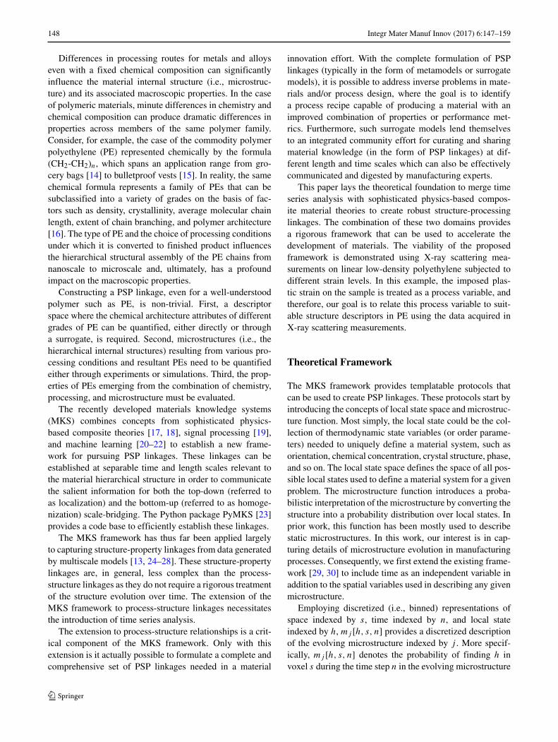
In Eq. 2, j [r, n] is a normalization factor that pro-vides a count of the total number of times it is actuallyfeasible to evaluate both mj [h, s, n] and mj [h′, s + r, n].This normalization factor can therefore depend on the dis-cretized vector r and the time step n (allowing for changesin the microstructure volume with time). A full set of two-point statistics is defined by all possible vectors that can bedefined within an image [13, 29, 33, 34]. Two-point statis-tics fj [h, h′, r, n] are most efficiently computed via discreteFourier transforms [29]. The transformation of materialstructure information into two-point statistics provides thebenefit of creating a natural origin or a point of reference(usually taken as r = 0) that can be used to objectively com-pare spatial arrangements of the local states across a givenmicrostructure as shown in Fig. 2.

Fig. 1 Idealized digitized microstructure with two local states shownby the white and gray voxels. The relative spatial locations for twovoxels are described by a discretized vector r

Creating structure-property linkages or classificationmodels with the raw two-point statistics is difficult dueto the large feature space and collinear features. Low-dimensional microstructure descriptors can be created usingdimension reduction techniques such as principal com-ponent analysis (PCA) or one of its variants [35, 36].PCA is a global unsupervised distance-preserving lineartransformation, which then finds its way naturally intothe known physics-based theories [37]. Additionally, accu-rate approximations to PCA are computationally fasterthan other dimensionality reduction techniques [38]. In theMKS framework, PCA is used to create low-dimensionalmicrostructure descriptors using linear combinations of thetwo-point statistics. Mathematically, this transformation canbe expressed as

fj [l, n] ≈K∑

k=1

μj [k, n]φ[k, l] + f [l] (3)

In Eq. 3, fj [l, n] is a feature vector that includes all two-point statistics deemed important for the problem (l indexesall unique combinations of h, h′, and r included in the anal-ysis; see [39] for guidance on how to make such selections)at time step n. As defined earlier, j identifies a particularmicrostructure evolution pathline. φ[k, l] and f [l] are theestimated time-independent PCs and the time-independentmean values of the selected features, respectively. K is thetotal number of PCs. μj [k, n] are the time-dependent PCscores and are taken as the low-dimensional descriptors for

150 Integr Mater Manuf Innov (2017) 6:147–159

Fig. 2 Discretizedmicrostructure (left) and itstwo-point statistics (right). Eachpixel in the two-point statisticsimage depicts the probability offinding the selected local statesat the ends of a vector whose tailis at the origin and the head is atthe pixel itself (Color figureonline)

microstructure evolution pathline j . Often, most of the vari-ation in a dataset can be captured by only a few PC scores.Let k = 1, 2, ..., K∗ denote this low-dimensional represen-tation of the microstructure, where K∗ is many orders ofmagnitude smaller than the large number of microstructurestatistics included in the analysis. Previous studies have suc-cessfully used these protocols to create structure-propertylinkages with effective properties or microstructure classi-fication models that could be used to objectively quantifythe variation in microstructures due to changes in manu-facturing processes [13, 29, 30, 34]. A related protocol forlocalization (i.e., top-down scale-bridging) has also beenapplied successfully to a variety of multiscale materialphenomena [12, 24–27, 32].

While previous MKS studies have successfully capturedstructure-property linkages, the application of the sameframework to establishing process-structure evolution link-ages requires the extensions developed and presented inthis paper. As noted earlier, this extension is specificallydesigned to facilitate the application of time series anal-ysis techniques. Time series modeling approaches can beseparated into methods that work in the frequency domainsuch as spectral analysis [40–42] and wavelets [43–45], andmethods that work in the time domain. The time domainmethods can be further separated into three main categories:autoregresive integrated moving average (ARIMA) mod-els [46], state space models [47–53], and non-parametricregression machine learning models [54–56], notably neuralnetworks.

ARIMA models were developed by Box and Jenkins[46] and predict the evolution of time series data basedon previous values and previous errors. The advantages ofARIMA models are that (i) the model has a relatively smallnumber of parameters, (ii) the parameters can be estimatedvia ordinary least squares, and (iii) the model itself andits parameters are relatively intuitive. The model requiresthat non-linear trends be removed from the data, and if theresiduals are normally distributed, simple estimates for thevariance-covariance matrix of the parameters are available[46].

State space models estimate a joint probability over latentstate variables and observed measurements. A Kalman Fil-ter [47] can be used when the latent state variable is assumedto be continuous, while hidden Markov models can be usedwith discrete latent variables [48–50]. State space modelscan be viewed as recursive Bayesian estimation [57] and arewell suited for streaming noisy data. The models create alinear function using a Markov assumption (only the pre-vious state is needed to predict the current state), althoughextensions of the models have been made to account fornon-linearities [51–53]. The drawbacks from this methodare that (i) the parameter estimation is non-convex and (ii)the dynamics of the system must be well understood a pri-ori to create transition models to update the latent statevariables.

Neural networks have been successfully applied to timeseries analysis as well as other sequential learning prob-lems. The most notable model is long short-term memoryneural network (LSTM) [54]. LSTM introduces the conceptof a memory block which contains gates that control theflow of information into and exiting the memory block aswell as information carried into the next time step [55]. Thismodel has been shown to outperform the previous two meth-ods with non-stationary data [56], but optimization of neuralnetwork parameters is non-convex and typically requires asignificant amount of data [55].

In this study, an extension to the MKS homogenizationframework is presented based on a non-parametric exten-sion to ARIMA models for time series data gathered fromsynchrotron based in situ X-ray scattering measurements. Inexperiments of this type, the material system under investi-gation is constantly exposed to an X-ray beam which allowsthe internal structure to be probed continuously. Simulta-neously, the thermodynamic state variables for the system,i.e., processing conditions, are perturbed and the resultingchanges in the properties of the material under investiga-tion are observed and recorded. These state variables caninclude temperature, pressure, and electric fields or theircombinations. Using this tri-component approach of simul-taneously monitoring structural changes continuously while

Integr Mater Manuf Innov (2017) 6:147–159 151

manipulating the process variables and recording the cor-responding properties permits the construction of a timeseries-based process-structure linkage. Although our worktowards establishing PSP linkages is demostrated on X-rayscattering data, the approach can be extended to data from insitu experiments utilizing a variety of microscopy, tomogra-phy, neutron scattering, and spectroscopic techniques.

Time Series Analysis for Process-StructureEvolution Linkages

State space models enjoy certain advantages in handlingnoisy data and can be adapted to in-line learning fromstreaming data. But in order to avoid divergence and mini-mize error, these models require a priori knowledge of thedynamics of the system to create state transition matrices.Although some work has been done to empirically calibratethese transition matrices [58, 59], the dynamics of low-dimensional microstructure descriptors is generally not wellunderstood. While LSTMs have shown significant predic-tive power when optimized with a large dataset, in manypractical applications, material datasets are not large enough[60]. For these reasons, LSTM and state space models werenot used in this study.

ARIMA models require information from previous pre-diction errors (at prior time steps). This makes multisteppredictions challenging with a moving average componentwhile autoregressive models only require information frompredictions at prior time steps. As a result, autoregressivemodels lend themselves better to multistep predictions. Anon-parametric regression method call multivariate adap-tive regression splines (MARS) was developed by Friedmen[61] and later applied to time series analysis by Lewis andothers [62, 63]. In time series applications, the method isreferred to as time series multivariate adaptive regressionsplines (TSMARS). TSMARS has been shown to work wellin a moderate dimensional setting (in our case, the numberof PCs is expected to be 20 or less) and moderate-sized data(between 50 and 1000 datapoints) [61].

In the present application, TSMARS will be used to esti-mate a function, F , connecting the current microstructuredescriptors μ[k, n] with their prior values as well as poten-tially with processing parameters η[n]. Mathematically, thisfunction can be expressed as

μj [k, n]=F(μj [k, n−1], μj [k, n−2], ...η[n], η[n−1], ...)+ε

(4)

In Eq. 4, μj [k, n − i] and η[n − i] are the microstructuredescriptor (i.e., kth PC score) and the processing parameter,respectively, at the discrete time step (n − i). The functionF is expressed as a linear combination of basis functions,

each of which is (i) a constant, (ii) a hinge function withknot point at an observed input location, or (iii) a prod-uct of the hinge functions. The coefficients in the series arecommonly estimated via least squares regression. A hingefunction can be defined as in Eq. 5, and an example of twohinge functions meeting at a knot equal to 5 is shown inFig. 3.

g(x) =

x, if x > 0.

0, otherwise.(5)

In the example used in this study, strain values correlatewith time steps (i.e., the same strain history is imposed onall samples); therefore, strain does not provide additionalinformation. Therefore, the function F will only be writ-ten in terms of the previous values of the microstructuredescriptors μj [k, n − i] for the remainder of the paper.

The TSMARS estimation consists of three major steps.

1 A forward pass greedily adds basis functions in mirrorimage pairs to minimize mean squared error (MSE) untila stopping criteria is reached.

2 A pruning or backward pass removes the least importantbasis functions greedily to avoid over-fitting accordingto generalized cross validation (GCV).

3 Coefficients for the basis functions are estimated usingleast squares.

Detailed explanations of MARS and TSMAR can be foundin published literature [61–63].

In this study, the iterations of the forward pass werestopped if (i) the R-squared value was greater than 0.999or (ii) the change in the R-squared was less than 0.001.The number of PCs, K , and the autoregressive order, P , arethe two hyper-parameters in the model development; thesewere optimized for the process-structure linkage extracted

Fig. 3 An example of two hinge functions meeting at a knot withvalue of five (κ = 5) (Color figure online)

152 Integr Mater Manuf Innov (2017) 6:147–159

in this work using a leave one sample out cross-validationapproach. When selecting the range over which to search,three practical issues need to be considered. (i) P deter-mines the number of initial images that need to be providedto the model at the time of prediction. As a result, a suf-ficiently accurate model with a low value of P is desired.(ii) As K increases, the amount of variation retained in thelow-dimensional microstructure descriptors μj [k, n] alsoincreases (i.e., we obtain a more complete description of themicrostructure). (iii) While the time complexity for predic-tion is O(NPK), where N is the number of time steps, thetime complexity for estimation is O

(N2(PK)3

). The last

two issues require an optimized value of PCs where a suf-ficient amount of the variation is captured without the runtime becoming too large.

During the cross-validation process, each of the sam-ples was systematically left out during the estimation of themodel parameters. After each of the estimations, the first P

images from the sample not used during the estimation wereprovided as initial conditions for the model. The predictionprocess recursively used predictions from the previous timesteps in the model (i.e., if P = 1, then μj [k, n + i] is usedto predict μj [k, n + i + 1]). The MSE values, as defined inEq. 6, were computed over the predicted time steps.

1

NK

K∑

k=1

N∑

n=1

(μj [k, n] − μj [k, n])2 (6)

Application

In a conventional synchrotron X-ray scattering experiment,the specimen under investigation is irradiated by a collimatedbeam of monochromatic X-rays. The incident X-rays inter-act non-destructively with the electrons in the specimen.This interaction results in a fraction of the X-rays deviatingfrom their original collimated path, i.e., results in scattering.The spatial distribution of electrons in a material, the elec-tron density distribution, is a characteristic of the material.In turn, the scattering of incident X-rays due to the electrondensity distribution is characteristic of that microstructure.The scattered X-rays, which are captured on a 2D detectorplate, create a 2D scattering pattern which contains the rel-evant microstructural information. Depending on the typeof X-ray scattering technique used for investigation, themicrostructure of a material can be characterized acrosslength scales spanning from 0.1 nm to 1 μm [64].

Small-Angle X-ray Scattering of Partially CrystallinePolymers

Small-angle X-ray scattering (SAXS) is a subset of X-ray scat-tering techniques wherein inhomogeneities or two-phase

microstructural features at the mesoscale between 1 nmand 100 s of nm can be probed in a specimen. In thiswork, we use SAXS to investigate the mesoscopic struc-ture of semi-crystalline polymer films of linear low-densitypolyethylene (LLDPE), a grade of PE. Semi-crystallinepolymers comprise of a microstructure wherein the poly-mer chains can organize into crystalline and non-crystallinedomains. The crystalline domains consist of tightly packedpolymer chains that have become regularly ordered to formlamellae while amorphous domains are formed from loosedisordered arrangements of the polymer chains. In an idealcase, the crystalline and non-crystalline domains are sepa-rated by a sharp interface, and therefore, the two domainscan be considered to be separate local states. Most impor-tantly, the electron density in crystalline domains, ρc, isgreater than the electron density in the amorphous domains,ρa .

A single SAXS pattern provides an average descriptionof all the spatial arrangements of crystalline and amorphousdomains within the scattering volume at that instant of time.The time series data used in this application of the MKShomogenization approach are image sequences of suchSAXS patterns obtained while simultaneously recording thestress and strain data of the individual specimens duringuniaxial tensile stretching. The dataset therefore providesinsight into the evolution of the semi-crystalline microstruc-ture at the mesoscale for different LLDPEs under uniaxiallyapplied stress and strain.

For this case study, X-ray scattering data serve as a surro-gate for two-point statistics. Mathematically, X-ray scatter-ings from a two-phase microstructure have been shown tocorrespond to the Fourier transform of the autocorrelationof the difference in electron density [65].

Table 1 Labeling of tensile specimens made from blown films of thetwo LLDPE polymers

Polymer Film label BUR Thickness (μm) Images

LLDPE1 LLDPE1.1a 2.5 20 182

LLDPE1.1b 2.5 30 191

LLDPE1.1c 2.5 75 195

LLDPE1.2a 3 20 191

LLDPE1.2b 3 30 195

LLDPE1.2c 3 75 191

LLDPE2 LLDPE2.1a 2.5 20 191

LLDPE2.1b 2.5 30 195

LLDPE2.1c 2.5 75 61

LLDPE2.2a 3 20 227

LLDPE2.2b 3 30 199

LLDPE2.2c 3 75 206

Integr Mater Manuf Innov (2017) 6:147–159 153

Materials and Methods

Melt blown films of two LLDPE polymers, henceforthreferred to as LLDPE1 and LLDPE2, were supplied byExxonMobil Chemical Company (EMCC). Both the LLD-PEs were statistical copolymers of ethylene and hexene,where the hexene comonomer was incorporated along thebackbone chain in the form of butyl short-chain branching(SCB). The densities for LLDPE1 and LLDPE2 were 0.912and 0.923 g/cm3. The density variation between the twopolymers arose from the differing levels of SCB incorpo-ration. The melt flow index for each of the polymers was1.0 (ASTM-D1238) and the molecular weight distributionsfor these LLDPEs were also similar. Both polymers wereconverted into films by the method of film blowing intotwo series of blown films. The first series of films had ablow up ratio (BUR) of 2.5 while the second series hada BUR of 3. The BUR is a standard processing parame-ter which describes the manufacture of blown films. Withineach series, three films were fabricated with average thick-nesses of 20,30, and 75 μm, thereby totaling 12 films. Thelabeling scheme followed in the current work to describetensile specimens for in situ testing is described in Table 1.

SAXS experiments were performed at beamline 12-IDCof the Advanced Photon Source (APS) at the ArgonneNational Laboratory (ANL). In these experiments, the

X-ray beam had an energy of 12 keV (i.e., a wave-length of 1.0332 A) and the beam dimensions were200 μm × 200 μm. X-rays scattered by the LLDPE filmspecimens were detected by a MAR CCD detector situ-ated at a distance of 2426 mm from the LLDPE specimen.The detector pixel size was 175 μm. A fixed exposure timeof 0.1 s was utilized while taking SAXS snapshots. SAXSpatterns were collected every 3 s. This time interval wasdetermined based on the minimum detector readout time perpattern. A portable tensile stage, made by Linkam ScientificInstruments, was utilized for the tensile measurements. TheLinkam stage was operated at a tensile deformation rate of25.4 mm/min. The collection of SAXS data and deforma-tion data was synchronized such that the first SAXS patternin any of the image sequences was always obtained from anunstrained pristine specimen at t0.

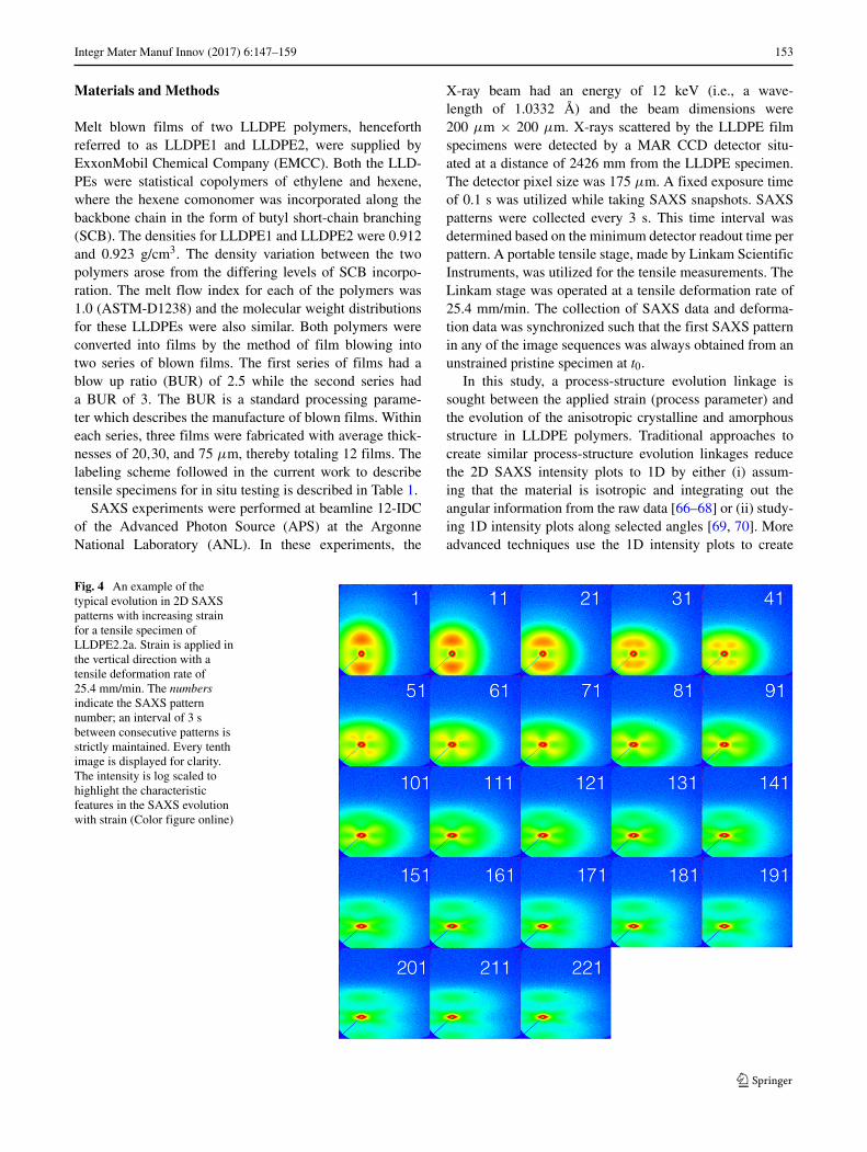
In this study, a process-structure evolution linkage issought between the applied strain (process parameter) andthe evolution of the anisotropic crystalline and amorphousstructure in LLDPE polymers. Traditional approaches tocreate similar process-structure evolution linkages reducethe 2D SAXS intensity plots to 1D by either (i) assum-ing that the material is isotropic and integrating out theangular information from the raw data [66–68] or (ii) study-ing 1D intensity plots along selected angles [69, 70]. Moreadvanced techniques use the 1D intensity plots to create

Fig. 4 An example of thetypical evolution in 2D SAXSpatterns with increasing strainfor a tensile specimen ofLLDPE2.2a. Strain is applied inthe vertical direction with atensile deformation rate of25.4 mm/min. The numbersindicate the SAXS patternnumber; an interval of 3 sbetween consecutive patterns isstrictly maintained. Every tenthimage is displayed for clarity.The intensity is log scaled tohighlight the characteristicfeatures in the SAXS evolutionwith strain (Color figure online)

154 Integr Mater Manuf Innov (2017) 6:147–159

Fig. 5 a Principal component scores for X-ray scattering images from the 12 different samples and b the percent variance captured as a functionof the number principal components (Color figure online)

2D collection functions to look at changes over time [71,72]. Indeed, all of these techniques are aimed at reduc-ing the dimensionality of the structure information obtained

from the scattering measurements. In the present study,we take an objective (data-driven) approach to dimen-sional reduction using the MKS framework described

Fig. 6 The mean and first five principal components computed doing principal component analysis on 2224 images. 86.7% of the variance in thedataset is captured by the first five principal components (Color figure online)

Integr Mater Manuf Innov (2017) 6:147–159 155

earlier. One of the main advantages of the MKS approachis that we can retain a significantly larger amount ofthe information in the reduced dimensional representa-tion of the microstructure with a remarkable ability torecover almost the full representation when needed. Thisis mainly because of the use of the PCA and storing theinformation on the PCs and the mean values of the fea-ture distributions, as will be illustrated later in this casestudy.

Data Processing

Prior to analysis, the contrast X-ray scattering images weretransformed by taking the log of the intensity. In order tonormalize the difference in intensity due to film thickness,each of the images was normalized by their mean intensityvalue.

PCA was done on the complete set (ensemble) of 2224images from the 12 samples (see Table 1). Each scatteringimage (such as those shown in Fig. 4) was represented asa vector of 422,500 intensities. In other words, the dimen-sionality of the measured structure information is 422,500,which is clearly unwieldy to extract high value process-structure evolution linkages. Figure 5b shows the explainedvariance in the complete ensemble of the measured struc-tures as a function of the number of PCs. This essentiallymeans that fewer than 20 PCs would be enough to recovermost of the original microstructure information. This isindeed a remarkable reduction in dimensions, from 422,500

to less than 20, while capturing 88% of the differencesbetween the individual structures in the ensemble. The fullensemble of structures is shown in the first three PCs inFig. 5a. In this visualization, the structure evolution ineach of the 12 samples is tracked by assigning distinctcolors and symbols to each sample. Consequently, we canvisualize the structure evolution in each sample as a singlepathline.

The mean and the first five PCs are reshaped from vec-tors into the original images and are presented in Fig. 6.As explained in Eq. 3, the image titled mean is the time-independent mean of the entire ensemble. Images titled PC1through PC5 identify the most distinguishing features inthe X-ray scattering images in an orthogonal frame. PC1appears to increase the contribution from short vectors, atthe expense of long vectors. PC2 appears to impart a largebias in the horizontal direction compared to the verticaldirection. The higher order PCs are capturing increasingcomplex features. The large dimension of each PC makes itvery difficult to understand all of the information embeddedin each component. Physical interpretation of the PCs in theMKS framework is a current area of major research interest.

Model Selection, Estimation, and Validation

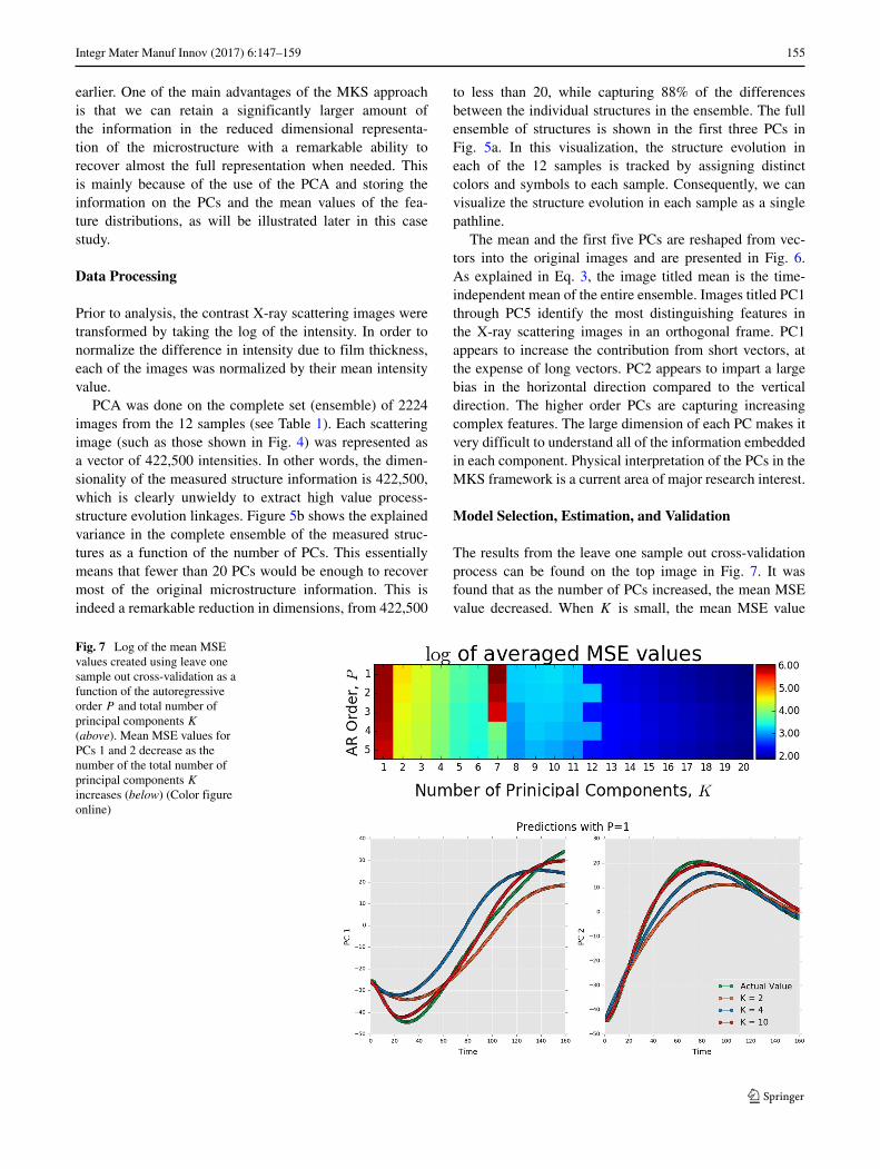
The results from the leave one sample out cross-validationprocess can be found on the top image in Fig. 7. It wasfound that as the number of PCs increased, the mean MSEvalue decreased. When K is small, the mean MSE value

Fig. 7 Log of the mean MSEvalues created using leave onesample out cross-validation as afunction of the autoregressiveorder P and total number ofprincipal components K

(above). Mean MSE values forPCs 1 and 2 decrease as thenumber of the total number ofprincipal components K

increases (below) (Color figureonline)

156 Integr Mater Manuf Innov (2017) 6:147–159

decreases as P increases, but this trend reverses as the K

gets large. In general, the value of P had less effect on theMSE value as the number of PCs increased. This essen-tially means that we are likely to extract a better modelby capturing in more detail the structure information in theimmediately preceding one to two timesteps as opposed toretaining less structure information over a larger number ofthe preceding timesteps. Indeed, the model with the lowestmean MSE value was found to have P = 1 and K = 20and had an average value of 6.8 overall all calibrations. Thegeneral trend indicates that the model accuracy would con-tinue to increase as the number of PCs increases but withdiminishing returns and higher computational costs. The

bottom images in Fig. 7 qualitatively show that the predic-tions for PCs 1 and 2 improve as the total number of PCs,K , increases.

In order to demonstrate the utility of this method, theresults from models with the maximum and minimum MSEvalues found during the cross-validation process for P = 1and K = 20 are shown in Figs. 8 and 9. Using the pre-dicted low-dimensional microstructure descriptors, a lowrank approximation of the X-ray scattering images wascreated as shown in Eq. 3. The model used to predictsample LLDPE1.2b had the lowest MSE value of 2.11.Figure 9 shows the actual final image and the final predictedimage using the reduced-order image as well as the entire

Fig. 8 Predicted and actual principal component scores for sample LLDPE1.2b (above). The original image (bottom left) and the predicted image(bottom right). The mean squared error value over the predicted principal component scores had a value 2.11 (Color figure online)

Integr Mater Manuf Innov (2017) 6:147–159 157

Fig. 9 Predicted and actual principal component scores for sample LLDPE2.2b (above). The original image (bottom left) and the predicted image(bottom right). The mean squared error value over the predicted principal component scores had a value 19.9 (Color figure online)

microstructure evolution pathline (in the PC space). Themodel used to predict sample LLDPE2.2b had a MSE valueof 19.9. The measured and predicted images are shown inFig. 9 along with the predictions of the entire microstruc-ture evolution pathline. Interestingly, in spite of the largedifferences in the error measures, both predictions in Figs. 8and 9 have retained the relevant scattering information.

Leave one sample out cross-validation was used in thisstudy for two reasons: (i) consideration of the least and mostaccurate models allows for an unbiased assessment of themethod’s utility and robustness, and (ii) leave one sampleout cross-validation is equivalent to a traditional train-testsplit where 11 samples are used to calibration and one sam-ple is used for validation, repeated 12 times in the presentcase study. Most practical material development efforts

have limited data, and this approach provides an excellentstrategy for building useful models with limited data.

Conclusion

In this paper, an extension of the MKS homogenizationframework is presented to allow extraction of process-structure evolution linkages from multiscale materialdatasets. This extension was accomplished by extendingthe definition of the discretized microstructure function toinclude details of its temporal variation. Most importantly,this extension was accomplished in a way that allowed thecontinued application of PCA for low-dimensional repre-sentation of the material structure and its time evolution in

158 Integr Mater Manuf Innov (2017) 6:147–159

a selected processing step as a structure evolution pathline.This is particularly significant as this is the only knowndimensionality reduction algorithm that employs a distance-preserving linear transformation, which allows a naturalinsertion into established composite theories (for establish-ing the complementary structure-property linkages) and iscomputationally low cost. Therefore, the framework pre-sented here potentially offers the broadest interoperabilitywith complementary PSP linkages needed to objectivelyguide the material innovation efforts. Furthermore, theframework presented here was amenable to the applica-tion of time series multivariate adaptive regression splines(TSMARS). The viability and potential of this extendedframework was demonstrated through an application on anensemble of small-angle X-ray scattering images obtainedfrom in situ plastic deformation of low-density PE sam-ples. It was seen that the proposed framework exhibitedremarkable accuracy in capturing the highly non-linearand complex characteristics of structure evolution in theseexperiments.

The theoretical framework outlined in this paper pro-vides a strong foundation to connect time series analysisand sophisticated composite theories to create robust process-structure evolution linkages. Together with process-structurelinkages, this method can be used to create comprehensiveprocess-structure-property linkages in a format that can bereadily accessed and utilized by the material developmentcommunity and shared with manufacturing experts.

Acknowledgments DBB and SRK acknowledge support from theNSF-IGERT Award 1258425 and NIST 70NANB14H191. AK andDGB acknowledge support from the ExxonMobil Chemical Company.

References

1. National Science and Technology Council Executive Office of thePresident: Materials Genome Initiative for Global Competitiveness.http://www.whitehouse.gov/sites/default/files/microsites/ostp/materials genome initiative-final.pdf Accessed 2011-06-30

2. Materials Genome Initiative National Science and TechnologyCouncil Committee on Technology Subcommittee on the Materi-als Genome Initiative: Materials Genome Initiative Strategic Plan.http://www.whitehouse.gov/sites/default/files/microsites/ostp/NSTC/mgi strategic plan dec 2014.pdf Accessed 2014-12-30

3. Allison J (2009) Integrated computational materials engineering(ICME): a transformational discipline for the global materialsprofession. Allied Publishers, New Delhi, p 223

4. Allison J (2011) Integrated computational materials engineering:a perspective on progress and future steps. JOM 63(4):15–18

5. Olson GB (2000) Designing a new material world. Science288(5468):993–998

6. On Integrated Computational Materials Engineering, N.R.C.U.C.Integrated computational materials engineering: a transforma-tional discipline for improved competitiveness and national secu-rity. National Academies Press, 2008

7. Schmitz GJ, Prahl U (2012) Integrative computational materialsengineering: concepts and applications of a modular simulationplatform. John Wiley & Sons

8. Robinson L (2013) TMS study charts a course to successful ICMEimplementation Springer

9. Panchal JH, Kalidindi SR, McDowell DL (2013) Key compu-tational modeling issues in integrated computational materialsengineering. Comput Aided Des 45(1):4–25

10. Kalidindi SR (2015) Data science and cyberinfrastructure: criticalenablers for accelerated development of hierarchical materials. IntMater Rev 60(3):150–168

11. Kalidindi SR, Gomberg JA, Trautt ZT, Becker CA (2015) Appli-cation of data science tools to quantify and distinguish betweenstructures and models in molecular dynamics datasets. Nanotech-nology 26(34):344006

12. Brough DB, Wheeler D, Warren JA, Kalidindi SR (2016)Microstructure-based knowledge systems for capturing process-structure evolution linkages. Curr Opinion Solid State Mater Sci,in press. doi:10.1016/j.cossms.2016.05.002

13. Kalidindi SR, Niezgoda SR, Salem AA (2011) Microstructureinformatics using higher-order statistics and efficient data-miningprotocols. JOM 63(4):34–41

14. Lajeunesse S (2004) Plastic bags. Chem Eng News 82(38):51

15. Faur-Csukat G (2006) A study on the ballistic performance ofcomposites, vol 239. Wiley Online Library, pp 217–226

16. Peacock A (2000) Handbook of polyethylene: structures: proper-ties, and applications. CRC Press

17. Kroner E (1986) Statistical modelling. Springer, pp 229–291

18. Kroner E (1977) Bounds for effective elastic moduli of disorderedmaterials. J Mech Phys Solids 25(2):137–155

19. Volterra V (2005) Theory of functionals and of integral andintegro-differential equations. Courier Corporation

20. Suits DB (1957) Use of dummy variables in regression equations.J Am Stat Assoc 52(280):548–551

21. Galton F (1886) Regression towards mediocrity in hereditarystature. J Anthropol Inst G B Irel

22. Cooley JW, Tukey JW (1965) An algorithm for the machine cal-culation of complex fourier series. Mathematics of computation19(90):297–301

23. Brough DB, Wheeler D, Kalidindi SR (2017) Materials knowl-edge systems in python—a data science framework for accelerateddevelopment of hierarchical materials. Integrating Materials andManufacturing Innovation, in press

24. Landi G, Niezgoda SR, Kalidindi SR (2010) Multi-scale modelingof elastic response of three-dimensional voxel-based microstruc-ture datasets using novel DFT-based knowledge systems. ActaMater 58(7):2716–2725

25. Kalidindi SR, Niezgoda SR, Landi G, Vachhani S, Fast T (2010)A novel framework for building materials knowledge systems.Computers, Materials, & Continua 17(2):103–125

26. Yabansu YC, Patel DK, Kalidindi SR (2014) Calibrated local-ization relationships for elastic response of polycrystalline aggre-gates. Acta Mater 81:151–160

27. Al-Harbi HF, Landi G, Kalidindi SR (2012) Multi-scale model-ing of the elastic response of a structural component made from acomposite material using the materials knowledge system. ModelSimul Mater Sci Eng 20(5):055001

28. Gupta A, Cecen A, Goyal S, Singh AK, Kalidindi SR (2015)Structure–property linkages using a data science approach: appli-cation to a non-metallic inclusion/steel composite system. ActaMater 91:239–254

Integr Mater Manuf Innov (2017) 6:147–159 159

29. Cecen A, Fast T, Kalidindi SR (2016) Versatile algorithms for thecomputation of 2-point spatial correlations in quantifying mate-rial structure. Integrating Materials and Manufacturing Innovation5(1):1–15

30. Cecen A, Fast T, Kumbur E, Kalidindi S (2014) A data-drivenapproach to establishing microstructure–property relationships inporous transport layers of polymer electrolyte fuel cells. J PowerSources 245:144–153

31. Yabansu YC, Kalidindi SR (2015) Representation and calibra-tion of elastic localization kernels for a broad class of cubicpolycrystals. Acta Mater 94:26–35

32. Fast T, Niezgoda SR, Kalidindi SR (2011) A new framework forcomputationally efficient structure–structure evolution linkagesto facilitate high-fidelity scale bridging in multi-scale materialsmodels. Acta Mater 59(2):699–707

33. Niezgoda SR, Yabansu YC, Kalidindi SR (2011) Understandingand visualizing microstructure and microstructure variance as astochastic process. Acta Mater 59(16):6387–6400

34. Niezgoda SR, Kanjarla AK, Kalidindi SR (2013) Novelmicrostructure quantification framework for databasing, visualiza-tion, and analysis of microstructure data. Integrating Materials andManufacturing Innovation 2(1):1–27

35. Hotelling H (1933) Analysis of a complex of statistical variablesinto principal components. J Educ Psychol 24(6):417

36. Mika S, Scholkopf B, Smola AJ, Muller K-R, Scholz M, RatschG (1998) Kernel PCA and de-noising in feature spaces, vol 4.Citeseer, p 7

37. Kalidindi SR (2015) Hierarchical materials informatics: novelanalytics for materials data. Elsevier

38. Halko N, Martinsson P-G., Tropp JA (2011) Finding structure withrandomness: probabilistic algorithms for constructing approxi-mate matrix decompositions. SIAM Rev 53(2):217–288

39. Niezgoda S, Fullwood D, Kalidindi S (2008) Delineation of thespace of 2-point correlations in a composite material system. ActaMater 56(18):5285–5292

40. Scargle JD (1982) Studies in astronomical time series analysis.II-statistical aspects of spectral analysis of unevenly spaced data.Astrophys J 263:835–853

41. Warner RM (1998) Spectral analysis of time-series data. GuilfordPress

42. Granger CWJ, Hatanaka M, et al. (1964) Spectral analysis ofeconomic time series spectral analysis of economic time series

43. Chan K-P, Fu AW-C (1999) Efficient time series matching bywavelets. IEEE, pp 126–133

44. Grinsted A, Moore JC, Jevrejeva S (2004) Application of thecross wavelet transform and wavelet coherence to geophysicaltime series. Nonlinear Process Geophys 11(5/6):561–566

45. Percival DB, Walden AT (2006) Wavelet methods for time seriesanalysis vol. 4. Cambridge University Press

46. Box GE, Jenkins GM, Reinsel GC, Ljung GM (2015) Time seriesanalysis: forecasting and control. John Wiley & Sons

47. Kalman RE (1960) A new approach to linear filtering and predic-tion problems. J Basic Eng 82(1):35–45

48. Baum LE, Petrie T (1966) Statistical inference for probabilis-tic functions of finite state Markov chains. Ann Math Stat37(6):1554–1563

49. Rabiner LR (1989) A tutorial on hidden Markov models andselected applications in speech recognition. Proc IEEE 77(2):257–286

50. Rabiner LR, Juang B-H (1986) An introduction to hidden Markovmodels. IEEE ASSP Mag 3(1):4–16

51. Julier SJ, Uhlmann JK (1997) New extension of the Kalman fil-ter to nonlinear systems. International Society for Optics andPhotonics, pp 182–193

52. Wan EA, Van Der Merwe R (2000) The unscented Kalman filterfor nonlinear estimation. IEEE, pp 153–158

53. Gustafsson F, Hendeby G (2012) Some relations betweenextended and unscented Kalman filters. IEEE Trans Signal Pro-cess 60(2):545–555

54. Hochreiter S, Schmidhuber J (1997) Long short-term memory.Neural Comput 9(8):1735–1780

55. Lipton ZC, Berkowitz J, Elkan C (2015) A critical review ofrecurrent neural networks for sequence learning. arXiv preprintarXiv:1506.00019

56. Pankratz A (2009) Forecasting with univariate Box-Jenkins mod-els: concepts and cases vol. 224. John Wiley & Sons

57. Masreliez C, Martin R (1977) Robust Bayesian estimation forthe linear model and robustifying the Kalman filter. IEEE TransAutom Control 22(3):361–371

58. Salti S, Di Stefano L (2013) On-line support vector regressionof the transition model for the Kalman filter. Image Vis Comput31(6):487–501

59. Haaland B, Min W, Qian PZ, Amemiya Y (2010) A statisticalapproach to thermal management of data centers under steadystate and system perturbations. J Am Stat Assoc 105(491):1030–1041

60. Kalidindi SR, De Graef M (2015) Materials data science: currentstatus and future outlook. Annu Rev MaterRes 45:171–193

61. Friedman JH (1991) Multivariate adaptive regression splines. AnnStat, 1–67

62. Lewis PA, Stevens JG (1991) Nonlinear modeling of time seriesusing multivariate adaptive regression splines (mars). J Am StatAssoc 86(416):864–877

63. De Gooijer JG, Ray BK, Krager H (1998) Forecasting exchangerates using TSMARS. J Int Money Financ 17(3):513–534

64. Narayanan T, Diat O, Bosecke P (2001) SAXS and USAXSon the high brilliance beamline at the ESRF. Nuclear Instru-ments and Methods in Physics Research Section A: Accelerators,Spectrometers. Detectors and Associated Equipment 467:1005–1009

65. Cebe P, Hsiao BS, Lohse DJ (2000) Scattering from polymers:characterization by X-rays, neutrons, and light. ACS Publications

66. Gurun B, Bucknall DG, Thio YS, Teoh CC, Harkin-Jones E (2011)Multiaxial deformation of polyethylene and polyethylene/claynanocomposites: in situ synchrotron small angle and wide anglex-ray scattering study. J Polym Sci B Polym Phys 49(9):669–677

67. Gurun B, Thio Y, Bucknall D (2009) Combined multiaxial defor-mation of polymers with in situ small angle and wide angle x-rayscattering techniques. Rev Sci Instrum 80(12):123906

68. Samon JM, Schultz JM, Hsiao BS, Seifert S, Stribeck N, GurkeI, Saw C (1999) Structure development during the melt spin-ning of polyethylene and poly (vinylidene fluoride) fibers by insitu synchrotron small-and wide-angle x-ray scattering techniques.Macromolecules 32(24):8121–8132

69. Guaqueta C, Sanders LK, Wong GC, Luijten E (2006) The effectof salt on self-assembled actin-lysozyme complexes. Biophys J90(12):4630–4638

70. Chmelar J, Pokorny R, Schneider P, Smolno K, Belsky P, KosekJ (2015) Free and constrained amorphous phases in polyethylene:interpretation of 1 H NMR and SAXS data over a broad range ofcrystallinity. Polymer 58:189–198

71. Noda I, Ozaki Y (2005) Two-dimensional correlation spec-troscopy: applications in vibrational and optical spectroscopy.John Wiley & Sons

72. Smirnova DS, Kornfield JA, Lohse DJ (2011) Morphology devel-opment in model polyethylene via two-dimensional correlationanalysis. Macromolecules 44(17):6836–6848