extraction of early perceptual structure in dot patterns...
TRANSCRIPT

COMPUTER VISION, GRAPHICS, AND IMAGE PROCESSING 48, 304-356 (1989)
Extraction of Early Perceptual Structure in Dot Patterns: Integrating Region, Boundary, and
Component Gestalt*
NARRNDRA AHUJA AND MIHRAN TIJCERYAN~
Coordinnted Science L&oratory, University of Illinois at Urbana-Champaign, 1101 West Springfield Avenue, Urbana, Illinois 61801
Received February 2,1987; revised May 26,1989
This paper presents a computational approach to extracting basic perceptual structure, or the lowest level grouping in dot patterns. The goal is to extract the perceptual segments of dots that group together because of their relative locations. The dots are interpreted as belonging to the interior or the border of a perceptual segment, or being along a perceived curve, or being isolated. To perform the lowest level grouping, first the geometric structure of the dot pattern is represented in terms of certain geometric properties of the Voronoi neighborhoods of the dots. The grouping is accomplished through independent modules that possess narrow exper- tise for recognition of typical interior dots, border dots, curve dots, and isolated dots, from the properties of the Voronoi neighborhoods. The results of the modules are allowed to influence and change each other so as to result in perceptual components that satisfy global, Gestalt criteria such as border and curve smoothness and component compactness. Such lateral communication among the modules makes feasible a perceptual interpretation of the local structure in a manner that best meets the global expectations. Thus, an integration is performed of multiple constraints, active at different perceptual levels and having different scopes in the dot pattern, to infer the lowest level perceptual structure. The local interpreta- tions as well as lateral corrections are performed through constraint propagation.using a probabilistic relaxation process. The result is a partitioning of the dot pattern into different perceptual segments or tokens. Unlike dots, these segments possess size and shape properties’ in addition t0 lOCatiOnS 8 19X9 Academic Press. Inc.
1. INTRODUCTION
The projection of the three-dimensional world onto two-dimensional images results in the loss of information such as depth. The true three-dimensional structure has to be recovered by the visual system from images that could have arisen from an infinite number of possible scenes. The recovery of the lost three- dimensional information cannot be done uniquely based on a geometrical theory alone, and additional assumptions are necessary.
For example, consider an image that contains two parallel lines. The parallelism could be the result of actual parallelism of two lines in three-dimensional space. Or, the parallel lines could be the projections of two parallel, planar curves viewed so that the planes containing the curves project as straight lines. This latter case is unlikely since it assumes an unstable viewpoint. In general, it appears safe to make the assumption that if two lines in the image plane are parallel, then they are also parallel in space, without requiring further data to verify that the image does not really result from an unstable viewpoint. Making this assumption eliminates the
*This research was supported by the Air Force Office of Scientific Research under Grant AFOSR 82-0317 and the National Science Foundation under Grant ECS-83-52408.
‘Currently at Dept. of Computer Science, Michigan State University, E. Lansing, MI 48824.
304 0734-189X/89 $3.00 Copyright c 1989 hy Academic Press, Inc. All rights of reproduction in any form reserved.

EXTRACTION OF PERCEPTUAL STRUCTURE 305
need of first obtaining a three-dimensional description of the lines, and then of testing whether they are parallel in three-dimensional space. This illustrates the use of image plane entities, and constraints on their image plane structure, to make inference about the three-dimensional scene structure directly, without involving any three-dimensional structural primitives, or using specific previous knowledge about the contents of the scene [19]. Significance of image plane structure is determined by image plane entities. Structurally related entities are said to be grouped.
Grouping thus means “putting items seen in the visual field together,” or “organizing” image data. The organization may be at different scales. The rules to detect some basic organizations may be completely stated in terms of intrinsic properties of tokens being grouped and their image plane relationships. This paper is concerned with grouping of simple image plane entities-dots in a dot pattern. The goal is to develop a set of rules as well as a computational process that makes use of the rules for identifying groupings of dots.
1.7.. Why Dot Patterns
‘The image entities, or tokens, that may be grouped include blobs and edge segments. These tokens have properties such as position, shape, size, orientation, color, brightness, and the termination points (if the tokens are elongated or curvilinear). The interaction between some of the properties may be complex resulting in conflicting groupings [16, 381. To reduce this complexity, a first step toward understanding the grouping phenomenon may be to study the roles of some relatively simple properties. One way of accomplishing this is to eliminate all but one property at a time and examine the effects of that property on grouping. Dot patterns provide a means of studying the effect of token positions on their grouping. With dots as tokens, the role of nonpositional properties is minimized since dots are without size, orientation, color, and shape. We call the initial grouping of dots based only on their positions as the lowest level grouping (Fig. 1).
This paper presents a computational approach to obtain the lowest level grouping in dot patterns. The simplicity of tokens holds only for this level of grouping. The segments or tokens defined by the lowest level grouping have spatial extent, and
‘. .‘:. . .
. . ::
‘._. _. I :’
__.. ,. .:
., ‘._ ;. . . .
::..
.
FIG. 1. An example dot pattern which illustrates a number of perceptual structures: an annular structure, a curvilinear structure, and two compact structures, one with a homogeneous interior density and one with a varying interior density.

306 AHUJA AND TUCERYAN
1.’ .‘:. . . . .
. . . . . . : . . : : .
. .
: . . : . : . .
; :
. . . . . . . . .
FIG. 2. An example pattern showing hierarchical grouping of tokens.
hence, properties such as orientation, shape, and size. For example, pairs of dots grouped together at the lowest level form virtual lines which behave similar to actual oriented line segments [20]. The lowest level tokens may further group hierarchically to yield groupings at higher levels. Figure 2 shows an example of hierarchical grouping. Such hierarchical grouping will not be addressed in this paper.
1.2. Characterizing Perceptual Structure
To define a computational approach to the lowest level grouping, it is necessary to specify what precisely is the desired output of the grouping process given the input dot pattern. Since the grouping is among dots, it should be possible to define the perceptual structure also with dots as elements of description. In such a description, each dot should have associated with it a component of the perceptual structure, or a perceptual role. The goal of the lowest level grouping process, then, is to assign to each dot its perceptual role. To see what roles a dot can play in the lowest level grouping, let us closely examine the process of grouping.
The single variable that determines the grouping of dots is the relative locations, or proximity, of dots. If the proximity is more pronounced in one or two directions, the result is a curvilinear structure of dots. If a dot has all its proximal dots occurring in a contiguous sector of its surround, and not just along one or two directions, then the dot lies along the border of a perceptual segment. This means that one side of the dot is empty relative to the other side. When a dot is completely surrounded by other dots, this indicates that the given dot lies in the interior region of a perceptual cluster. The surrounding dot density in such a case may be uniform or variable. One last possibility is the case in which a dot has no other dot in its proximity. Such an isolated dot gives rise to a single-dot cluster. Thus, the possible perceived structures are: (a) a cluster with nonempty interior, (b) a cluster with no interior (e.g., a bar), (c) curvilinear structures, and (d) a single-dot cluster. In the first case a dot may lie either along the border of a cluster or in the interior region. The goal of the computation of the lowest level groupings may be achieved by assigning to each dot one of the above roles, or, one of the following labels: INTERIOR, BORDER, CURVE, and ISOLATED. Except for the CURVE label, this set of labels is the same as the one used by Zucker and Hummel [44].
1.3. Overview of the Work Presented
The work described in this paper aims at defining and implementing a computa- tional approach to obtaining lowest level grouping in dot patterns. It is not the intention here to model the grouping mechanisms used by the human visual system. Rather, the goal is only to achieve the same groupings as perceived by humans using

EXTRACTION OF PERCEPTUAL STRUCTURE 307
steps which may or may not have analogs in human visual processing. These steps may well be motivated by known psychophysical results, but they are adapted for their computational feasibility. Specifically, these steps resolve issues such as:
(a) How should the geometric structure of a dot pattern be represented? (b) How is the local perceptual structure related to the local geometric struc-
ture? (c) How is the extraction of structure influenced by nonlocal constraints? (d) How to integrate constraints that arise at different levels?
Answering such questions leads toward the definition of a computational ap- proach. The performance of the approach will be judged by the end result, namely, how close the groupings produced are to those perceived by humans. We now present a brief overview of the approach presented in this paper.
The lowest level grouping extracts the perceptual segments of dots that group together because of their relative locations. The grouping is accomplished by interpreting dots as belonging to interior or border of a perceptual segment, or being along a perceived curve, or being isolated. To perform the lowest level grouping, first the geometric structure of the dot pattern is represented in terms of certain geometric properties of the Voronoi neighborhoods of the dots (Section 4). It is argued that the Voronoi neighborhoods serve as a “natural” representation of the local perceptual structure of dots. The geometric properties are then related to the primitives of the perceptual structure, e.g., interiors of blobs, borders of blobs, curves, and isolated dots. The grouping is seeded by assigning to dots their locally evident perceptual roles and iteratively modifying the initial estimates to enforce global Gestalt constraints (Section 5). This is done through independent modules that possess narrow expertise for recognition of typical interior dots, border dots, curve dots, and isolated dots, from the properties of the Voronoi neighborhoods. The results of the modules are allowed to influence and change each other so as to result in perceptual components that satisfy global, Gestalt criteria such as border or curve smoothness and component compactness. Such lateral communication among the modules makes feasible perceptual interpretation of the local structure in a manner that best meets the global expectations. Thus, an integration is performed of multiple constraints, active at different perceptual levels and having different scopes in the dot pattern, to infer the lowest level perceptual structure. The local interpretations as well as the lateral corrections are performed through constraint propagation using a probabilistic relaxation process. The result of the lowest level grouping phase is the partitioning of a dot pattern into different perceptual segments or tokens.
A major theme of the work presented in this paper is integration of multiple constraints to detect the basic perceptual structure of a dot pattern. The constraints that are integrated include those due to local structure of dots, smoothness of borders, and compactness of components. Starting with the first constraint which is due to the local structure, the next two constraints incorporate information having increasingly global (spatial) scope in the dot pattern. This distinguishes the work presented here from much previous work on dot patterns (Section 2). In the implementation of the approach, we have attempted to minimize the use of ad hoc thresholds for decision making. Whenever possible, we have tried to increase the

308 AHUJA AND TUCERYAN
amount of information used, to reduce any ambiguity in interpretation. The thresholds used are listed in Appendix A. Many of these thresholds are adaptive. That is, they are specified as bounds on the allowed statistics of local, structural characteristics of the dot pattern, rather than as absolute numbers. Before we go on to describe our approach, the next section briefly reviews related previous work.
2. A SUMMARY OF PREVIOUS WORK
Although our goal in this paper is to present a computational approach to the lowest level grouping (which is not designed to model the mechanisms involved in any similar processing in human vision) it should be noted that interest in grouping processes originated with work in psychology. The Gestalt psychologists in the 1920s and 1930s appear to have been the first to study grouping extensively as part of the general process of perception [16, 381. Gestaltists formulated a set of rules to explain the groupings perceived by humans. These rules were typically justified by drawing parallels with certain neurological theories that were known at the time, and in terms of such physical phenomena as electromagnetic fields. Many psy- chophysical experiments on various aspects of grouping processes in human vision followed. Following are examples of some recent experiments.
Uttal et al. studied how detection of lines formed by dots on a noisy background is affected by interdot spacing [34]. Glass et al. studied the perception of global structure in Moire patterns (formed by superposing on a dot pattern a transformed version of itself) as a function of the global transformation, e.g., dilation, rotation, or translation [ll-131. There have also been studies on temporal groupings [3, 41. Recent computational work on grouping has been significantly influenced by the psychological findings. Since our interest in this paper is limited to only computa- tional approaches, we will not review the work in psychology any further. To summarize the past computational work, we will first overview the work on clustering algorithms for partitioning dot patterns. Then we will review the more recent work on perceptual organization.
2.1. Clustering
Usually, the clustering problem is not formulated in a modular form such as suggested by the four questions we raised in Section 1.3. For example, our first two questions imply computation of geometric structure as a precursor to estimation of the perceptual structure. Similarly, the next two questions imply separate computa- tion of and potential conflict between, the locally computed structure and the globally perceived structure. A large number of clustering algorithms do a one-stage extraction of the clusters via optimization of some global objective function of interobject distances. Graph theoretic algorithms constitute a small exception to this general characterization of clustering algorithms; these algorithms incorporate inter- dot distances for a subset of all possible pairs of dots defmed by some notion of neighbors. But, other questions are ignored by these algorithms like the rest of the clustering algorithms. In this section, we will review some common approaches to clustering.
Clustering algorithms have been developed for a long time. Given a set of points, P, clustering is partitioning of P into subsets or classes that maxim&s both the similarity among members of the same subset, and dissimilarity across classes [8]. The points usually have vector attributes and are located in a multidimensional

EXTRACTION OF PERCEPTUAL STRUCTURE 309
feature space. The performance of a clustering algorithm is determined by the power of the similarity (or the homogeneity) measure employed. The clustering algorithms can be easily used on two-dimensional data, the case of interest to us in this paper.
To define specific approaches to clustering, several issues must be addressed. First, since the only basis of clustering is the relative position information of nearby dots, a notion of “nearbyness”, or “neighbors” and “neighborhood” of a point must be devised. Second, a measure of “similarity” among the members of a single cluster must be defined, depending on the particular application and what is considered a natural partition of the data. Third, an algorithm must be developed which uses this information to actually perform clustering.
Some common algorithms compute the clusters to minimize some objective function. Others, perform clustering using the spatial adjacency information or neighbors of dots. The concept of the “neighbors” of a dot for clustering has been defined in many ways in the past. Going from simple to complex, the different definitions include: the dots that fall into a circular neighborhood [25]; k-nearest neighbors [35, 441; O’Callaghan’s definition, which, in addition to distances of points, also incorporates relative orientations of points and information on whether a dot is hidden from another dot [23]; the minimum spanning tree used by Zahn [41] in which the two dots are neighbors if they are connected by an edge in the minimum spanning tree of the set of points; the relative neighborhood graph and the Gabriel graph used by Urquhart [33] and Toussaint [30]; and finally the Voronoi tessellation and its dual, Delaunay graph, recently described by Ahuja [l] and used in this paper. While the first two definitions have been used as ad hoc definitions of neighbors for clustering, the remaining graph based definitions are motivated by perceptual considerations, especially the last definition in terms of the Voronoi tessellation. A sound approach to extracting global, perceptual organization must have a sound definition of local structure. A detailed discussion of the advantages and disadvantages of the various notions of “neighbor” mentioned above, and the advantage of using “neighborhoods” can be found in [l].
Given a definition of neighbor, the clustering algorithms perform partitioning using two criteria: (a) a measure of similarity indicating if given tokens belong to a single cluster and (b) a criterion to decide when a given clustering is a good fit to the given data.
The different measures of similarity used in these algorithms may be based on the distance between dots, or they may be defined as the inner products of feature vectors associated with dots, depending on what is appropriate for that particular domain, and what constitutes a natural grouping for the given data. The different criterion functions for deciding when a particular partition is a good fit to data include sum of squared errors, minimum variance criteria, different (within cluster, between cluster) scatter matrices, and various scalar measures computed from them. A clustering algorithm typically performs some sort of iterative optimization on the set of data using the above mentioned criteria. A review of such clustering criteria and techniques can be found in [7, 81.
Other clustering techniques do not use the standard optimization procedures. Two major classes of such algorithms consist of the hierarchical clustering algo- rithms and graph-theoretical clustering algorithms. The hierarchical algorithms are usually implemented in one of two ways: (a) agglomerative algorithms which start with the individual samples as singleton sets and combine the clusters recursively to
310 AHUJA AND TUCERYAN
get larger sets, which, if repeated, eventually results in a single cluster containing the entire data; (b) divisive algorithms which start with the entire sample set as one cluster, and successively divide each cluster into smaller clusters which, if repeated, eventually results in each sample point being put into a separate cluster. Of course, the recursive splitting or merging may stop at any stage when a “stable” clustering has been achieved.
Graph theoretical algorithms start with a certain graph structure defined on the data set, and using criteria based on the properties of that graph eliminate the graph edges, thus splitting the set of points into subsets. In this sense, the graph theoretic clustering algorithms are similar to the divisive hierarchical clustering algorithms. Examples of the applications of these can be seen in [33,41].
2.2. Perceptual Organization
A major characteristic of clustering algorithms is that they assign a cluster to each dot, but they do not usually distinguish between dots belonging to a single cluster, for example, border dots and interior dots. Often the clustering is done in a high-dimensional feature space. In contrast, extraction of perceptual organization in dot patterns concerns the partitioning or clustering of dots in the original (planar, or sometimes three- or four-dimensional) space, and the measures of cluster homogene- ity are motivated by perceptual considerations. An obvious goal of computational approaches to perceptual organization is to develop algorithms to perform Gestalt clustering. Among the existing clustering algorithms, Zahn’s algorithm mentioned in the previous section takes perhaps the most perceptual structure oriented approach 1411.
To detect perceptual organization requires that all four questions raised in Section 1.3 be addressed. Typically, the previous work has not considered the third and the fourth questions. The answers to the first question (about the ways of representing geometric structure) are fundamentally limited in variety. Consider, for example, the problem of detecting perceptual organization in dot patterns. In this regard, the approach of Zucker and Hummel [44] illustrates some salient differences between clustering algorithms and algorithms that detect perceptual organization. Corre- sponding to our first question, they identify the different roles that a dot can play in a segment, namely whether it lies on the border or in the interior, or is isolated. We use the additional role of a dot being along a curve, which as we have argued, makes the resulting set of roles complete. With regard to the third and fourth questions, they enforce only local constraints [44, 431. In particular, the constraints used by them assign dot labels such that nearby dots have consistent interpretation. The enforcement of gestalt constraints such as border smoothness is, at best, indirectly achieved in their case through iterative application of local smoothness constraint; similarly, components of dots are not identified, and as a consequence, no global constraints are used for enforcing component compactness or closure. These con- straints are necessary since the perceptual roles of dots are determined by both local and global structure.
In the work presented in this paper, we integrate constraints at three levels: local (dot) level, border level, and component level. Further, we use a perceptually significant definition of local structure of a dot pattern which avoids the use of pattern specific thresholds; we use the Voronoi neighborhood of a dot, described by

EXTRACTION OF PERCEPTUAL STRUCTURE 311
Ahuja [l], as the starting point. Other differences between our work and the previous work will be pointed out in Section 7.
Usually, the differences in the range of nonlocal constraints employed distinguish different perceptual organization algorithms. Marr points out the need for percep- tual clustering algorithms to obtain full primal sketch from the raw primal sketch, by grouping tokens in the raw primal sketch using criteria such as collinearity and size simiIarity [20]. The problem of detecting perceptually salient smooth contours in dot patterns is also examined by Fairfield [9, 101 and Vistnes [36]. Zucker discusses the role of grouping processes in segmenting images in a manner such that image tokens grouped comprise a single three.-dimensional surface. Zucker argues that a major goal of the early processing in the human visual system is that of grouping image tokens to detect oriented structures [45, 461. He considers these oriented structures to be the fundamental constructs for visual processing that follows token extraction, e.g., symmetry detection, shape from texture, and spatio- temporal grouping. He distinguishes between two kinds of grouping processes: one that groups image tokens belonging to uniform interiors of surfaces, and another that is responsible for extracting tokens along smooth surface contours. He uses dot patterns to illustrate these processes.
An even higher level of image organization corresponds to groupings that capture three-dimensional perspective or other three-dimensional features. A good example of the grouping criterion used by such algorithms is nonaccidentalness. Rock has argued that many perceived organizations such as figure-ground and form corre- spond to groupings that are unlikely to have risen from accidental alignments or viewpoints [27]. We see the same ideas discussed by Witkin and Tenenbaum [39] and Lowe [19]. Lowe has made some of these criteria concrete and used them to build a vision system in which groupings among image tokens (not just dots) are based on the likelihood of their occurrence in perspective views of three-dimensional scenes.
2.3. Image Segmentation
In this section we contrast the problem of low level image segmentation with that of lowest level grouping in dot patterns. The goal of lowest level grouping in dot patterns is the same as that of pixel grouping in low level segmentation of gray scale or color images. In each case, the result is a description of the original data in terms of homogeneous segments. In fact, two major approaches to image segmentation: (a) region merging (growing) [5, 14, 21, 18,40,42] and (b) region splitting [6,24, 261 are analogous to the agglomerative and divisive clustering algorithms discussed in Section 2.2. Many image segmentation +gorithms do regard the problem as one of clustering of (feature) vectors representing pixel properties upon which the cluster- ing is based. The homogeneity criterion for dot clusters must involve geometric measures of dot locations which do not necessarily occur along a regular grid. On the other hand, images are defined on a regular grid, therefore homogeneity must depend on pixel gray level, color, texture, etc. Thus the two problems differ in the way the first two questions of Section 1.3 are answered.
The last two questions of Section 1.3 are equally important for both problems. The need for identifying pixels which he along the segment border or interior, etc. is no different for image segmentation than for identifying dots playing similar roles in dot patterns; this need is dictated by the process of segmentation and not by the

312 AHUJA AND TUCERYAN
type of data being segmented. The various local and global constraints discussed for dot patterns are equally significant for image segmentation. Therefore, low level image segmentation should benefit from the use of the Gestalt rules of perceptual organization such as border smoothness and compactness. However, with few exceptions [S], such organizational rules are usually not incorporated in low level segmentation algorithms (if we disregard the Gestalt rule of closure, which is automatically enforced because every detected region by default has a boundary around it even if it is not smooth). General low level image segmentation can be based on a variety of features that we have not mentioned so far in this paper, e.g., optical flow and texture. Which feature is used for segmentation depends upon what is available and what the goal of segmentation is; for example, segmentation of rigid objects could be done from optical flow images. Whatever the purpose of segmenta- tion, once image tokens are extracted the problem can be viewed, in part, as one of dot pattern segmentation, with dots representing the image tokens. Some of the goals of segmentation may be achieved by a one stage grouping while others require recursive grouping of the lowest level segments of dots.
3. REPRESENTING GEOMETRIC STRUCTURE
This section presents answers incorporated in our approach to the first two questions raised in Section 1.3: how the geometric structure is represented (Sections 3.1, 3.2) and how it is related to the local perceptual structure (Section 3.3). In Section 1 we saw that dot patterns comprise of shapeless tokens whose positions are of utmost importance. In reality the dots are not abstract points; they have finite sizes and shapes. However, if the shapes of all the dots in a pattern are the same and the separation between individual dots is sufficiently large compared to the dot diameters then the phenomenal effect of each dot is that of a point with no shape. The resulting percepts from such stimuli, therefore, are based effectively on the relative positions of the dots.
As we mentioned in Section 1, the dots interact with each other locally, i.e., direct relationships among the relative positions is important only for nearby dots. This interaction and perceived structure change when a sufficient number of intervening dots is introduced (Fig. 3). Therefore, it appears to be sufficient to capture only the local geometric environment, or the geometric structure, around a dot in a basic representation. In our approach, this geometric structure then serves as input to a procedure that infers perceived structural components such as blobs, borders, and curves, or the perceptual structure of a dot pattern. The geometric structure represents an abstraction of the dot pattern that captures all details of the dot pattern relevant to the inference of perceptual characteristics. It helps divide the problem of extracting perceptual description into two relatively loosely coupled
FIG. 3. The dots in (a) are perceived as a line segment. However, when included among many other dots that locally interact with the collinear dots, the perception of collinearity is lost (b) [19].

EXTRACTION OF PERCEPTUAL STRUCTURE 313
components. The perceptual component has access to the information in the dot pattern mainly through the geometric structure. It is thus crucial to have a sound notion and representation of the geometric structure-a representation that cap- tures all raw information of perceptual relevance.
3.1. Neighborhood of a Dot
As reviewed in Section 2, a major part of the past research on dot patterns has identified neighboring dots instead of assigning a two-dimensional neighborhood to a dot as proposed in [l]. The latter approach truly captures the local geometric environment of a dot, more than just identifying the neighbors of a dot. It allows access to the properties of a two-dimensional region around a dot in question such as area and shape properties. Such properties appear to play a central role in characterizing the geometric structure around a dot. For example, the area of a dot’s neighborhood is related to local dot density; variations in the area in different directions around dot reflect directional sensitivity of dot density; shape properties of the neighborhood are related to various aspects of the geometric perceptual structure (see Section 3.3). In contrast, when only neighbors of a dot are given, only properties such as distances between dots may be used which capture a hybrid of one- and two-dimensional information. The definition of neighbors requires the use of ad hoc parameters such as a fixed number (k) of neighbors [35, 441, or a fixed radius [25], or thresholds on angular locations of a neighbor [23]. The use of a neighborhood lends a fully two-dimensional character to the problem in that the dot pattern is converted into a planar image or mosaic which is important since dot pattern analysis of the kind we are interested in here regards dot patterns as two-dimensional images.
3.2. Voronoi Neighborhood
We use the Voronoi tessellation of a dot pattern to associate with each dot its neighborhood, even though two-dimensional neighborhoods can be assigned to dots in many ways (e.g., radius neighborhood). In this definition, the geometric proper- ties of the Voronoi neighborhoods represent the geometric structure of the dot pattern [l]. As one part of the geometric environment, the Voronoi neighborhoods also specify the neighbors of a dot. Before we discuss the representation of geometric structure further, we first review the definition of the Voronoi tessellation of a dot pattern.
Suppose that we are given a set S of three or more points in the Euclidean plane. Assume that these points are not all collinear, and that no four points are cocircular. Consider an arbitrary pair of points P and Q. The bisector of the line joining P and Q is the locus of points equidistant from both P and Q and divides the plane into two halves. The half plane Hg(Hi) is the locus of points closer to P (Q) than Q (P). For any given point P a set of such half planes is obtained for various choices of Q. The intersection flpG s, p+ ,, HP defines a polygonal region consisting of points closer to P than any other point. Such a region is called the Voronoi [37] polygon associated with the point. The set of complete polygons is called the Voronoi diagram of S [29]. The Voronoi diagram together with the incomplete polygons in the convex hull define a Voronoi tessellation of the entire plane. The Voronoi tessellation for the example pattern in Fig. 1 is shown in Fig. 4. Two points are said to be Voronoi neighbors if the Voronoi polygons enclosing them share a

314 AHUJA AND TUCERYAN
FIG. 4. The Voronoi tessellation of the dot pattern shown in Fig. 1.
common edge. The dual representation of the Voronoi tessellation is the Deluunuy graph which is obtained by connecting all the pairs of points which are Voronoi neighbors as defined above.
We consider as the neighborhood of a point P (the region enclosed by) the Voronoi polygon containing P. This choice of neighborhood definition was guided by the following advantages that the Voronoi neighborhood offers over various other definitions mentioned in Section 2. The fixed radius neighborhood, k-nearest neighbors, and O’Callaghan’s definition have parameters that need to be specified, whereas the Voronoi neighborhood definition is parameter-free. Unlike fixed-radius neighborhood definition, it is adaptive to scale and density variations. Unlike k-nearest neighbors definition, the number of neighbors is not fixed and the neighbor relation between dots is symmetric. The Voronoi neighbors of a point are not necessarily its nearest neighbors. Conversely, there may be points in the nearest neighbors set of a given dot which are not its Voronoi neighbors if they are hidden by other points [l]. The various other graph-theoretic definitions of neighbors such as minimum spanning tree (MST) [41] and relative neighborhood graph (RNG) [33, 301 are subsets of the Delaunay graph (DG). Therefore, the DG, and hence, the Voronoi neighborhood contains all the information contained in MST and RNG, and more. The points linked in MST may be considered neighbors. The neighbor relationship so defined, however, is based on global criteria and a small change in one region of the dot pattern can cause a change in the graph in a completely unrelated region. Therefore, the neighbor set in the MST is not very stable with respect to small local perturbations. The two dimensional neighborhood assigned to dots by RNG is less intuitive than the Voronoi neighborhood since the Voronoi polygon of a dot actually encloses that part of the plane which is closest to the dot, a “natural” neighborhood of the dot. In the case of the MST no such neighborhood is assigned to the dot.
3.3. From Voronoi Neighborhoods to Geometric Structure
Many of the perceptually significant characteristics of a dot’s environment are manifested in the geometric properties of the Voronoi neighborhoods. We would like to relate the three perceptual roles of dots INTERIOR, BORDER, and CURVE to appropriate geometric properties of the Voronoi neighborhoods, so we may infer

EXTRACTION OF PERCXPTUAL STRUCTURE 315
the perceptual roles from observed geometric properties. Let us first consider the INTERIOR label. By observing a number of dot patterns we have identified salient attributes of interior dots as the following: (a) complete surroundedness of the dot by other cluster dots, (b) the magnitude of dot density, (c) the isotropicity or directional variation in dot density, (d) the spatial rate of change of (nonstationary) density. The dominant attribute of the BORDER dots is that (e) they are sur- rounded systematically by neighbor dots only on the interior side of the cluster; the other directions lead to intercluster space. The dots on a CURVE are (f) spaced close together compared to their distances to their other neighbors. Finally, we require (g) a perceptually valid notion of the neighborliness of two dots which is necessary in defining (a-f) above. We have expressed each of these perceptual descriptions (a-g) in terms of geometric properties of the Voronoi neighborhoods. These properties are discussed in the following paragraphs, labeled (a-g). The specification of these geometric properties comprises our representation of the geometric structure of the dot pattern.
It is entirely likely that an alternate set of geometric properties would capture the same perceptual characteristics. We lay no claim to uniqueness or optimality of the properties we have chosen. In fact, since the purpose is to extract perceptual structure whose mathematical definition is unknown, it is not clear to us if any given set of properties could be tested for optimality. Perhaps under certain models of dot pattern structure one could enforce orthogonality of the information content of the various properties to select a smallest set of properties, but no such models are known.
We will use interchangeably the terms po@gon and neighborhood, the latter being the two-dimensional area surrounded by the Voronoi polygon. All of the measures described except the areas of the polygons are within the range 0 to 1. The eccentricity and elongation have directional information attached to them. In the case of eccentricity this information indicates the direction in which the density increases. Elongation includes the orientation of the major axis of the polygon. Some of the properties are based on the set of shape statistics called the moments of area.. For example, the property area is the zeroth order moment; eccentricity is computed from the first-order moments. Other properties, such as the compactness measure or the Gabriel measure, are related to higher order moments, although our computation of these properties proceeds directly from the geometry without computing the moments unlike the area and eccentricity computation.
(a) Compactness. The first property is the compactness, or regularity, of the Voronoi polygons. It distinguishes interior points from other points. In the interiors of clusters the points are surrounded relatively uniformly by other points. This results in relatively equal angles subtended on a dot by its neighboring dots which are themselves neighbors (Fig. 5). Thus the interior cells are “compact”. Now consider the cells in the region where borders of two clusters approach each other. The outside of a cluster border has a nonuniform distribution of dots, whereas the interior side has a uniform distribution. This results in the dot distribution around a point lying on a border segment to be uneven which leads to a wedge-like, or noncompact, Voronoi polygon. An example of such a case is the point A and its Voronoi neighborhood illustrated in Fig. 4. The computation of the compactness measure is shown in Fig. 5

316 AHUJA AND TUCFXYAN
j ‘1
o!
*
P aI
jt
FIG. 5. The compactness measure is computed in terms of the angles ak. Let a,,, = (&, a, - a,,)/(/ - 1). Then the compactness of the cell for point i, wi = (u,, - a,,,)/s.
(b) Area. The second property is the area of a Voronoi polygon of a dot. It measures the magnitude of the dot density in the vicinity of the dot. Recalling the way the Voronoi tessellation is constructed, clusters with uniform density will result in the Voronoi neighborhoods having equal areas in the interior of such clusters. In clusters with varying density, the areas of the Voronoi neighborhoods will decrease along the direction of increasing dot density.
(c) Elongation. The third property of the Voronoi cells is meant to distinguish clusters having isotropic density from those in which the density is direction sensitive. For clusters with anisotropic density, the Voronoi polygons tend to be elongated. The major and minor axes of the polygons indicate the directions of the smallest and the largest densities, respectively. The cells along a curve also tend to be elongated since the dot density is much lower on the two sides of the curve compared to along the curve (as illustrated by point B in Fig. 4). There are many ways the elongation of a polygon can be computed. One possibility is the ratio of the area of the polygon to its perimeter squared. Another, which we have used, is based on the moments of the area. The elongation is computed by first identifying an ellipse (having major axis, a, and minor axis, 6) which has the same second order moments as the Voronoi
i-+
olygon. The elongation of the Voronoi polygon is then computed as 1 - (b/u) . The expression for the elongation in terms of the moments of area p20, pll, and po2 of the Voronoi polygon is
[ 0 c20 - co2)* + 4c:1y2 l/2
elong = ((p, - Po212 + 4EL:y2 + P20 + PO2 1 .
(d) Eccentricity. The eccentricity of the Voronoi polygons indicates the direction and magnitude of the density change. The width of the Voronoi polygons in the direction of increasing density decreases by an amount proportional to the density change. Further, the positions of the dots are also off the center of gravity of their respective Voronoi polygons, shifted in the direction of increasing density. The eccentricity measure is a scaled vector indicating how much and in which direction a dot is off the center of gravity of its Voronoi polygon. The computation of eccentricity is shown in Fig. 6. The interiors of uniform clusters are expected to have cells with very low eccentricities. The eccentricity vectors of the cells in the interiors
EXTRACTION OF PERCEPTUAL STRUCTURE 317
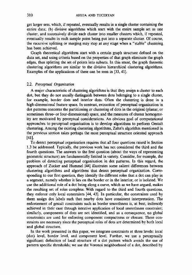
FIG. 6. Eccentricity of a cell belonging to point P is defined as d/D. Eccentricity direction is in the direction of QP. Here Q is the centroid of the cell.
of clusters having density gradients are expected to be aligned. At the borders of clusters, the eccentricity directions will point towards the interiors of the clusters because of the sudden increase in the dot density, i.e., from the very low density in the intercluster space to the comparatively high density in the interior of the cluster. This observation also holds on the borders of bars which are clusters without interior points.
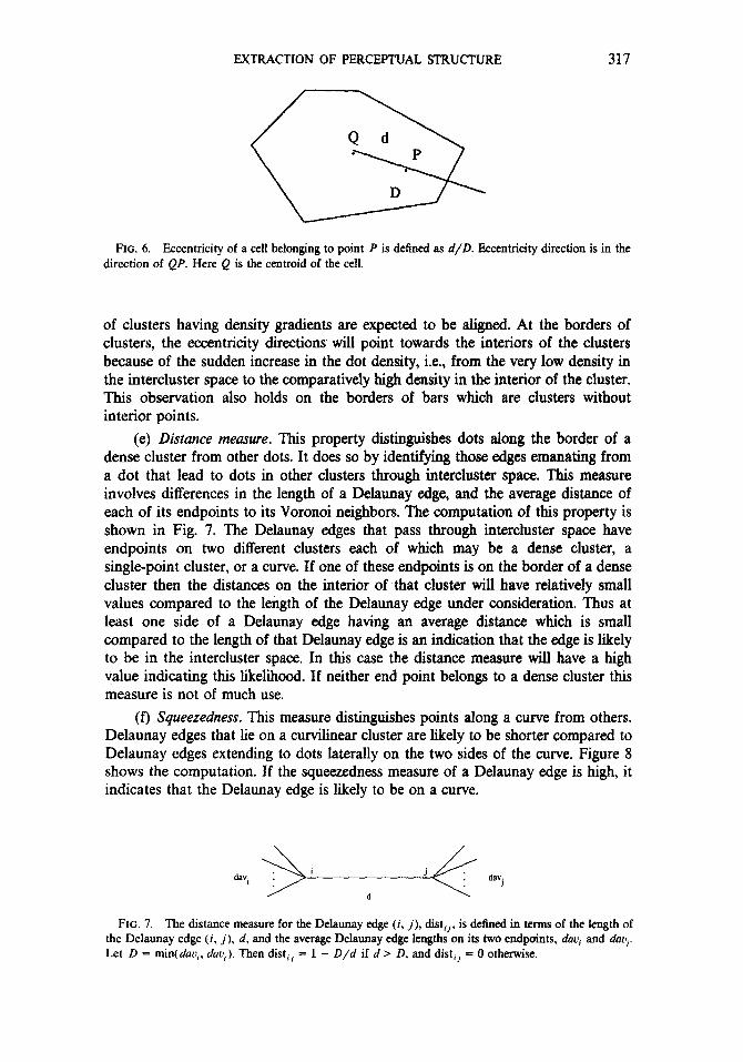
(e) Distance measure. This property distinguishes dots along the border of a dense cluster from other dots. It does so by identifying those edges emanating from a dot that lead to dots in other clusters through intercluster space. This measure involves differences in the length of a Delaunay edge, and the average distance of each of its endpoints to its Voronoi neighbors. The computation of this property is shown in Fig. 7. The Delaunay edges that pass through intercluster space have endpoints on two different clusters each of which may be a dense cluster, a single-point cluster, or a curve. If one of these endpoints is on the border of a dense cluster then the distances on the interior of that cluster will have relatively small values compared to the length of the Delaunay edge under consideration. Thus at least one side of a Delaunay edge having an average distance which is small compared to the length of that Delatmay edge is an indication that the edge is likely to be in the intercluster space. In this case the distance measure will have a high value indicating this likelihood. If neither end point belongs to a dense cluster this measure is not of much use.
(f) Squeezehess. This measure distinguishes points along a curve from others. Delaunay edges that lie on a curvilinear cluster are likely to be shorter compared to Delaunay edges extending to dots laterally on the two sides of the curve. Figure 8 shows the computation. If the squeezedness measure of a Delaunay edge is high, it indicates that the Delaunay edge is likely to be on a curve.
FIG. 7. The distance measure for the Delaunay edge (i, j), dist,,, is defined in terms of the length of the Delaunay edge (i, j), d. and the average Delaunay edge lengths on its two endpoints, duq and duo,. Let D = min(duo,, durr,). Then dist,, = 1 - D/d if d > D, and distii = 0 otherwise.

318 AHUJA AND TUCERYAN
FIG. 8. The squeezedness measure, sqij, is defined in terms of the Delaunay edge (i. j), d, and the average Delaunay edge lengths on its two sides, dav, and da+ Let D = min(a’av,, dav2). Then ~9,~ = 1 - d/D if d < D, and sqij = 0 otherwise.
(g) Gabriel measure. The final property is Gabriel measure which measures the “neighborliness” of two Voronoi neighbors. If the line joining two Voronoi neigh- bors i and j intersects the edge shared by the corresponding Voronoi polygons then i and j are perfect neighbors. If, on the other hand, there is a third point k such that the line (i, j) crosses the Voronoi cell for point k, then i is invisible from j because of the intervening Voronoi polygon of point k (Fig. 9). The deeper the line (i, j) penetrates cell k, the worse the neighbors (i, j) are and the lower the Gabriel measure is. This is important on the borders of clusters, where if the two points are not perfect neighbors and have a low Gabriel measure, then the border follows through the intervening point instead of directly connecting the two points. For example, in Fig. 9 if Gabriel measure is sutkiently low, the border passes through points (i, k, j) instead of going through (i, j) directly.
4. LOWEST LEVEL GROUPING
Perception of structure in dot patterns amounts to an assignment of structural roles to dots. In Section 1 we argued that the different roles that a dot could play are INTERIOR, BORDER, CURVE, and ISOLATED. Thus the goal of a computa- tional approach to perceptual grouping may be accomplished by assigning one of these roles to each dot.
To reiterate how these labels are selected, we enumerate possible contexts in which a dot can occur in any dot pattern. To do this, we start with a single dot and add points around it systematically and in each case identify the perceptual role of the original dot. Clearly, the label ISOLATED is justified for the initial dot. Now
FIG. 9. The Gabriel measure for the Delaunay edge (i, j): ga6qj = d/D if the line (i, j) intersects the line (k, V), and gabc, = 1 otherwise.

EXTRACTION OF PERCEPTUAL STRUCTURE 319
we start adding new dots. If we add a single dot as the neighbor of the original dot, we have a pair of dots that are perceived as along the border of a thin cluster or along a short curve. Therefore, either of the labels BORDER or CURVE is justified. If we add more points such that the points lie along the curve and the two “semiplanes” on the two sides of the original dot are empty, then again, the label CURVE is appropriate. Further, if we add more points on one side of the curve so that the original dot now is surrounded by close neighbors on that side, then the curve becomes part of the border of the cluster defined by the dots. In this case the label BORDER is justified. Finally, if we add more dots so that the original dot is surrounded on all sides, then the label INTERIOR is justified.
This set of labels should be complete in describing the lowest level perceptual structure. Other, more complex structures, could be defined in terms of these structural primitives. For example, consider a FORK junction where three curves meet. Here each dot could be considered as lying along one of the three curves. The FORK itself is the result of hierarchical grouping of curves. Extraction of such hierarchical groupings is beyond the scope of this paper.
4.1. The Need for Integration
What determines the perceptual role of a dot? In Section 3 we discussed how the different perceptual roles of a dot co-occur with characteristic local geometric structures. However, this association is only typical. The presence of a certain local geometric structure is neither necessary nor sufficient for a certain perceptual interpretation of a given dot-the local geometric structures of other dots, near and far, and their perceptual interpretations have a profound and usually domineering influence on how the given dot is perceived. “Faults” in the expected local geometric structures of a limited number of dots are tolerated in favor of Gestalt properties such as smoothness of borders or curves, or compactness of components, thus resulting in global interpretations that may assign such perceptual roles which conflict with their local geometric structures.
The multiplicity and diversity of constraints governing the final perceptual role of a dot require an integrated treatment of these constraints: While the interpretation process for a dot must be seeded by its local geometric structure in a bottom-up manner, no firm interpretation may be made until similar tentative bottom-up interpretations have been carried out elsewhere, and it is determined which interpre- tations are coherent; i.e., they satisfy expectations about global structure.
4.2. An Integrated Approach to Lowest Level Grouping
We now describe an approach to the lowest level grouping that uses constraints from different levels of structure; the immediate two-dimensional geometric envi- ronment of a dot, the shape of any border to which the dot may belong, and the shape of the component containing the dot. These three levels of constraints lead to the three steps of the grouping process illustrated in Fig. 10. AlI steps use analysis that is invariant of the scale as well as orientation of the dot pattern. The interpretation of dots depends only on their relative locations. The first step (box A in Fig. 10) consists of three independent modules (boxes II, BI, and CI) running in parallel. Each of these modules detects a primitive of the perceptual structure. The first one (II) identifies interior dots, the second one (BI) identifies border dots, and the third one (CI) identifies curves. Each of these modules possesses fairly limited

320 AHUJA AND TUCERYAN
, Input I Pattern .__________________ ------s
I I I Interior Border CUNC I I Identi6cation ldentificaticm Identification
(11) @I) (CO
FIG. 10. The various modules and control flow for the lowest level grouping.
,. . . . . . . :.Qg ,. .‘. .
C.-c !
. ‘. Q. .: :.: : . ..‘. ._“’ . . . .
I :
. ..,‘,
0 ,.y., .
FIG. 11. The output of the interior identification (II) module for the pattern in Fig. 1. The dots that lie inside the closed borders are labeled as INTERIOR. All the dots that lie either on the borders or outside the borders are labeled NONINTERIOR.

EXTRACTION OF PERCEPTUAL STRUCTURE 321
‘:I FIG. 12. The output of the border identification (BI) module for the pattern in Fig. 1.
expertise about how to recognize only its own perceptual primitive. The expertise is, of course, in terms of the expected geometric structure which is expressed in terms of the local geometric properties of the Voronoi neighborhoods given in the previous section. Because of the narrowness and spatial locality of this expertise, each module makes errors in detection. However, where one module may not find enough evidence for a decision, another may be very confident in its decision. Thus, modules may complement each other in the strengths and weaknesses of their performance. The second step (B) compares the results of the modules (II) and (BI) to correct possible errors that might exist in their results individually, thus combin- ing the strengths of the two modules. The correction is done by perturbing the output of each module such that smoothness of the borders as well as agreement among the modules are maximized. This mutual cooperation and strengthening is carried further into the third step where the already detected borders are used to identify potential components, or regions, of dots. Interpretations of dots and edges are modified so that they result in compact components having smooth borders. Thus the third step (C) combines the results of the border correction (BC) and interior correction modules (IC) based upon more global criteria. If a point receives low probabihty values for each of the labels INTERIOR, BORDER and CURVE, then it is given the label ISOLATED. To illustrate, the outputs of alI these modules obtained for the sample pattern in Fig. 1 are shown in Figs. 11-17. We have used
.,I. .. .: .:. ..“.-\ :’
‘:-; FIG. 13. The output of the curve identification (CI) module for the pattern in Fig. 1.
322 AHUJA AND TUCERYAN
. . . . .
;51’
:.Qcq .’ .” : $-?J 1.: :
+ :, . . .‘.. . . .
.:.
0 . .,‘.‘, . : .
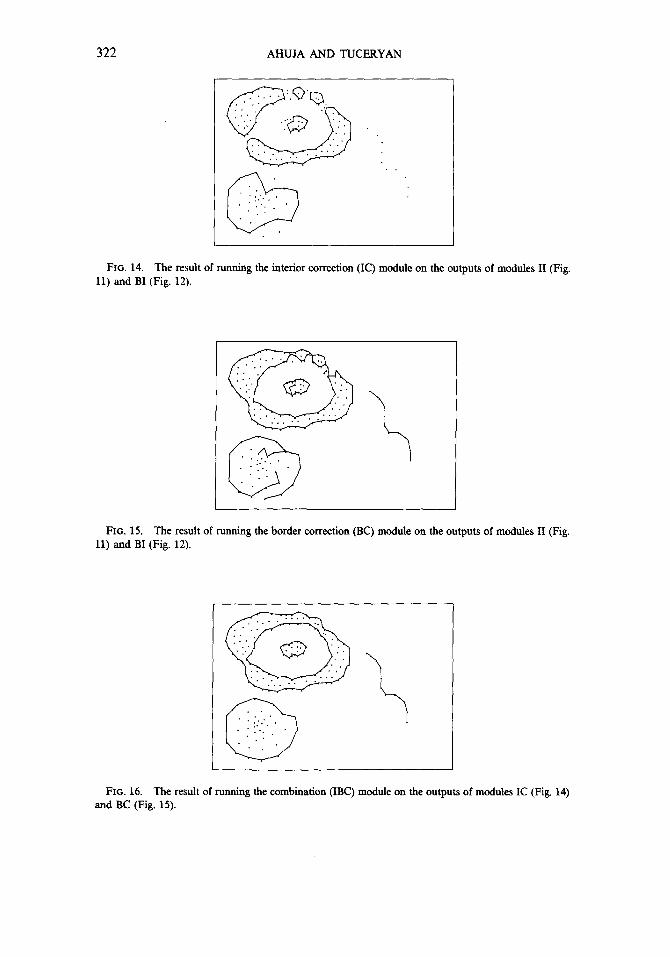
FIG. 14. The result of running the interior correction (IC) module on the outputs of modules II (Fig. 11) and BI (Fig. 12).
.’ . . . . . . ..’ .:::“’ @ r’,:: Q .’ .: . . . .. . . . . . a . . y,’ . . . . . ‘; FIG. 15. The result of running the border correction (BC) module on the outputs of modules II (Fig.
11) and BI (Fig. 12). . . . . . . . . . . m ,:,I .‘. @ ‘.:,:: . . ..’ . . . . .’ . .:.. .
0
. f 1’:. _’ .
“-, FIG. 16. The result of running the combination (IBC) module on the outputs of modules IC (Fig. 14)
and BC (Fig. 15).

EXTRACTION OF PERCEPTUAL STRUCTURE 323
c . 1 f : : . : ‘- _ ; ;.
:. c ?\ . . . . .* .”
..I r-: :. \:. .‘.
: r . ‘c-
:_,.: ‘; :
_’ ,’ ‘,__ , ;: I.; .y
. . ,.
. . :,. . ‘.. . . ‘:
.::, . .
FIG. 17. The result of running the curve correction (CC) module on the outputs of modules CI (Fig. 13), BC (Fig. 15). and IBC (Fig. 16).
the relatively sparse pattern of Fig. 1 to illustrate the role of each module since it contains several different perceptual components including curve and dense clusters even though the pattern has a relatively simple structure. The final results of the lowest level grouping for other relatively more complex patterns, though any single one of which may not contain all of the above components, are given later.
A powerful feature of this approach is the use of distributed expertise among modules. The limited expertise of the individual modules makes them computation- ally efficient, even though they lack in correctness of results. The latter problem is alleviated by strong lateral communication among modules. The lateral communica- tion enforces the Gestalt expectations on the interpretations of dots provided by the modules, to synthesize the correct, combined interpretation. Modules of successive stages use Gestalt properties of higher complexity, e.g., starting with curve proper- ties at the first stage and moving to component properties at the next.
5. ALGORITHM
To define an algorithm for the lowest level grouping, we need to answer the following questions. How do we relate the locally perceived role of a dot to its geometric structure? What are the Gestalt constraints on the interpretations of different dots? How does a formal inference procedure combine the information in geometric structure and the Gestalt constraints to identify the perceptual structure?
The first question concerns relating a dot’s role to its geometric structure. The measures we discussed in Section 4 represent different attributes of a dot related to its perceptual role. These attributes must be appropriately combined to obtain evidence in support of a given perceptual role of the dot. It needs to be determined exactly how the attribute values must be mapped onto the different perceptual roles. Further, only a fluid interpretation is desired at this stage since the interpretation will be subject to further revision when global constraints are taken into account. Thus, we should define functions of attributes such that the function values reflect only the degrees to which a dot acts as different perceptual entities instead of assigning a single role to the dot. We have chosen these functions to yield numerical

324 AHUJA AND TUCERYAN
values between 0 and 1 indicating the strength of a perceptual role that a dot performs. The function may be viewed as the probability that the dot is the given perceptual entity, since the values of the function are required to sum up to 1 over all perceptual roles. The net result of the local geometric analysis is then a probability vector assigned to each dot whose elements are the likelihoods of the dot fulfilling various perceptual roles based on local evidence.
The second question is about how the Gestalt constraints restrict the allowed spatial configurations of different perceptual elements such that they have desirable global characteristics. For example, the local interpretations (probabilities) of a set of dots being along a curve will be strengthened if the dots actually lie along a smooth curve. Similarly, the probabilities that a set of dots are border dots will be strengthened if the dots lie along a smooth curve and surround a compact compo- nent. The Gestalt constraints thus relate to both one-dimensional and two-dimen- sional aggregations of dots. Clearly, to enforce such constraints not only curves and borders must be extracted, but even connected components of dots must be identified. This implies multiple levels of analysis of dot pattern which must be performed on tentative interpretations, the latter subject to change as a result of the analysis.
The third question concerns the specification of a process of inference that would utilize the global constraints discussed in the second question to refine the interpre- tations obtained in answering the first question. Such a process must combine the probabilities of the various perceptual roles of a dot, each having a value between 0 and 1, with similar probabilities for the remaining dots, to obtain the probabilities of globally supported roles, each having a value between 0 and 1. The mutual interaction among the dots is according to the Gestalt constraints. In many cases, the result of the global interaction can be simulated by iterative local interaction. Thus, a dot’s probability vector may be modified based on the probability vectors of the dots in the immediate vicinity, with successive iterations of the process achieving spatial propagation of a dot’s influence.
We will now describe our current implementation of the lowest level grouping. We will do so by summarizing the basic implementation of each module shown in Fig. 10; the details of the implementation can be found in [31]. Each module uses probabilistic relaxation for inference, therefore, we will first briefly review the relaxation labeling process.
5 .l . Relaxation Labeling
Relaxation labeling is a technique of parallel constraint propagation for obtaining locally consistent interpretations (labels) of a class of objects [28]. When the context allows multiple interpretations of a single object, the (probabilistic) relaxation process orders them according to their likelihoods. The local consistency of interpre- tations of objects is based on a priori knowledge about the way objects interact.
Formally, we have a collection of objects ai, i = 1,. . . , n, and a set of labels Xi, i- ,..., 1 m. Each object has a set of probabilities pj(Xj), assigned to it that represent the likelihood of object a, having label X j, where Cj pi( X j) = 1. Each object is assigned a set- of initial probabilities, pf”)(Xj) as described later in this section. Then, the probabilities are updated iteratively, obtaining a new set of

EXTRACTION OF PERCEPTUAL STRUCTURE 325
probabilities after each iteration. The most commonly used updating formula is [28]
py+ I)( A) = pjk’(h)[l + qyyh)]
pek’(W + 4!kYvl~
where
&j(X, A’)J$~~(~‘) . A’ 1
The term rij( A, h’) in the last expression represents the compatibility of labels X and A’ on objects ai and aj, respectively. The dij’s are weights associated with the interaction of the pair of objects czi and aj, where Xj dij = 1, in order to keep the probabilistic properties of pi. Thus qjk)( h) represents the support given to the label h at the object a, by all the neighbors aj of a,.
At this point a few words need to be said about why we chose to use probabilistic relaxation labeling to implement our algorithm. We use relaxation because: (i) it naturally supports the use of local interactions between neighboring objects to enforce more global constraints such as border smoothness, (ii) by allowing different kinds (e.g., INTERIOR and BORDER) of processes to influence the probability of the same interpretation, relaxation provides a mechanism for continuous and cooperative interaction among different constraints on perceptual structure which is a major goal of our approach, and (iii) it minimizes or delays the use of arbitrary thresholds; when such thresholds are necessary, a general purpose threshold is used that does not depend upon parameters of the input patterns such as interdot distances, etc. For example, using local properties such as the directions of pairs of Delaunay edges we can enforce simple border smoothness. After settling on a locally consistent set of labels, we can use a global threshold on the resulting probabilities.
5.2. Interior Identijcution
The interior identification is formulated as a probabilistic relaxation process with dots being labeled as either INTERIOR or NONINTERIOR. This information is based upon the local geometrical properties of the Voronoi neighborhoods. This task., of course, is only meaningful if the clusters of dots have nonempty interiors.
The major step is to formulate the local compatibilities between pairs of dots in terms of the geometric properties of their polygons. Specifically, in the interiors of homogeneous clusters, the areas of Voronoi polygons are approximately the same and the eccentricities of the cells are low. In the interiors of nonhomogeneous clusters the eccentricities are high but they are pointing in the same direction, namely, in the increasing density direction. These facts, used conservatively, will result in the most obvious interior dots being identified. Those local regions where there might be noise effects on the positions of the dots even though they are in the interior of a segment, will either be classified erroneously or the labeling will not be confident.

326 AHUJA AND TUCXRYAN
The relaxation compatibilities are defined for the four possible combinations as two dots, i and j, namely (1) INTERIOR,INTERIOR,, (2) INTERIOR;NONIN- TERIOR,, (3) NONINTERIOR,INTERIORj, and (4) NONINTERIOR,-NON- INTERIOR,. In order to define these compatibilities we have to consider all the possible contexts in which a given combination of labels can occur. For example, all possible contexts in which different combinations of INTERIOR and NONINTE- RIOR can occur are as follows: The two points can be in the interior of either a homogeneous or a nonhomogeneous cluster. One point can be in the interior of either a homogeneous or a nonhomogeneous cluster and the other on the border. Both points can be on the border of the same cluster or the two points can be on the borders of two different clusters. For each of these cases an expression is written which summarizes the context through use of relevant geometric properties that characterize the given context. For example, in the case of two dots occurring in the interior of a homogeneous cluster a possible expression for the contribution of this context to the compatibility of INTERIOR-INTERIOR is
min(1 - ecc,,l - ecci,l - Aij).
In the expression ecci and eccj are the eccentricity magnitudes for the Voronoi polygons of the cells of dots i and 1, respectively. Aij is the area difference of the two polygons normalized to the range [0, l] and is defined as Aij = abs( Ai - Aj)/ max( Ai, Aj), where A, and Aj are the areas of the polygons for the dots i and j, respectively. The intuitive meaning of the expression is that in the interior of a homogeneous cluster the eccentricity magnitudes and the area differences are expected to be small. If that is the case with the two given dots, then expression (1) will have a high value and will have a positive contribution to the INTERIOR- INTERIOR compatibility value. After the expressions for all cases in which labels INTERIOR-INTERIOR occur have been derived, the expressions are combined by a fuzzy OR operation. In particular, for two dots i and j to be compatible with labels INTERIOR-INTERIOR, they must have the context of being in the interior of either a homogeneous cluster or a nonhomogeneous cluster. Similarly, expressions are obtained for other combinations of labels for the two dots and then combined to obtain label compatibilities.
Once the compatibilities have been defined, relaxation labeling is performed to assign to each dot probabilities of being INTERIOR or NONINTERIOR (step A, module II in Fig. 10). Most of these probabilities converge to either very high or very low values resulting in unambiguous labelings (even though they may be the wrong labels). In case of the few dots that have ambiguous probabilities, we assign them the label with the stronger probability. If this turns out to be the wrong label, the later phases will correct this, taking into consideration a larger context (step B in Fig. lo), information coming from other independent modules and Gestalt assump- tions such as border smoothness (steps B and C, and closure (step C).
5.3. Border Identijcation
The borders are the segments of curves that surround interior regions of dots. The surrounded interior region might be nonempty and contain dots labeled as INTE- RIOR or it might be empty in which case the dot cluster is a bar-like structure.
EXTRACTION OF PERCEPTUAL STRUCTURE 327
ecc1 ecc2 EXlWiM I , Extwim
J 4 0 0
,-\ ,*\ o ,‘el’x /’ ‘\
L ” o ,e1\ ,
\ e2 LO
” ‘,o ‘\ #’ \ s’
‘\ ,’ \ c2 I 8 i5
3 ‘6’ Interior
Interior
Interior
Cc)
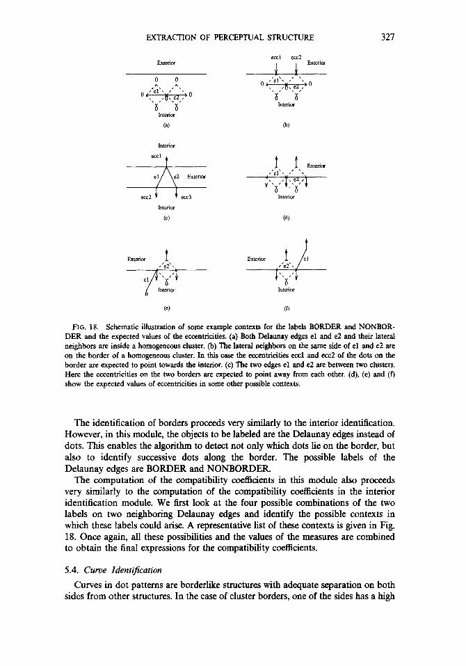
FIG. 18. Schematic illustration of some example contexts for the labels BORDER and NONBOR- DER and the expected values of the eccentricities. (a) Both Delaunay edges el and e2 and their lateral neighbors are inside a homogeneous cluster. (b) The lateral neighbors on the same side of el and e2 are on the border of a homogeneous cluster. In this case the eccentricities cccl and ecc2 of the dots on the border are expected to point towards the interior. (c) The two edges el and e2 are between two clusters. Here the eccentricities on the two borders are expected to point away from each other. (d), (e) and (f) show the expected values of eccentricities in some other possible contexts.
The identification of borders proceeds very similarly to the interior identification. However, in this module, the objects to be labeled are the Delaunay edges instead of dots. This enables the algorithm to detect not only which dots lie on the border, but also to identify successive dots along the border. The possible labels of the Delaunay edges are BORDER and NONBORDER.
The computation of the compatibility coefficients in this module also proceeds very similarly to the computation of the compatibility coefficients in the interior identification module. We first look at the four possible combinations of the two labels on two neighboring Delatmay edges and identify the possible contexts in which these labels could arise. A representative list of these contexts is given in Fig. 18. Once again, all these possibilities and the values of the measures are combined to obtain the final expressions for the compatibility coefficients.
5.4. Curve Identification
Curves in dot patterns are borderlike structures with adequate separation on both sides from other structures. In the case of cluster borders, one of the sides has a high

328 AHUJA AND TUCERYAN
density of dots whereas the other side usually has a large amount of empty space. Curves are well separated from other dots on both sides.
Curve identification is similar to border identification. The Delaunay edges are the objects to be labeled, with labels CURVE or NONCURVE.
The computation of compatibility coefficients is also similar to the case of border identification. The contexts for the curvilinear structures are different than the borders, and the compatibility expressions are computed accordingly.
5.5. Label Corrections to Enforce Agreement and Border Smoothness
As a result of the previous step (step A in Fig. lo), the dots and the Delaunay edges are labeled as INTERIOR-NONINTERIOR, BORDER-NONBORDER, or CURVE-NONCURVE. Some of these labels may not be correct due to lack of local evidence, ambiguities, etc. These incorrect labels need to be corrected by using information from a larger context. The results of the modules (II, BI, and CI) and their comparison provide part of the necessary information from a larger context. In addition, the criterion that borders be smooth is also used to decide whether a labeling of a dot or a Delaunay edge needs to be corrected. The context that is considered is larger because, for example, a border segment which is expected and constrained to be smooth extends beyond the neighborhood of the dot or Delaunay edge being considered for correction. Similarly, if the results of the different modules are forced to agree, this involves combination of information from different contexts.
Before going into the details of the algorithm for correcting the labels at this step, there is a minor representational point to be clarified. In the interior identification module the dots are labeled as INTERIOR or NONINTERIOR, but there is no explicit border information, which is needed in order to make the appropriate cross comparisons between the outputs of II and BI modules. In order to get comparable representations for the outputs of both modules, the interior regions identified by the II module are surrounded by borders. Except for clusters with empty interiors, this transformation makes it meaningful to speak about agreement between the two results, for example, by computing the fractions of border segments that are shared by the outputs of the two modules. Similarly, the transformation makes it feasible to enforce smoothness of borders in the interior identification module. The clusters with empty interiors, i.e., bars and isolated dots, do not have any interior dots and hence no border edges are provided by the II module. Therefore, there is no way to compare the two sets of output in these cases and they are handled separately in the interior-border combination module (IBC) in the next step.
The label correction step consists of two modules (IC and BC in Fig. 10). Each one concurrently and independently corrects one set of labels from the previous step using the information from the previous step as shown in Fig. 10. Not all of the dots or the Delaunay edges are considered for correction. The most confident ones (i.e., the dots or Delaunay edges whose identifications from the two independent modules II and BI are in agreement) are omitted. Only the objects whose identifications from the two independent modules conflict are considered for correction. This increases the efficiency of the correction process. A module changes the labels of its input if doing so improves the measure of border smoothness and increases agreement with the results of other modules. Some representative contexts for each set of inputs coming from the previous stage and the effect of changing label are shown in

EXTRACTION OF PERCEPTUAL STRUCTURE 329
FIG. 19. Some examples illustrating the details of label correction. The dashed lines represent non border Delaunay edges and solid lines represent border Delaunay edges. Cases (a) and (b) demonstrate the effect of changing the label of a point by the interior correction (IC) module. In (a) when the label for point i is changed from NONINTERIOR to INTERIOR, the change is reflected in the border around it as shown in (b). Cases (c) and (d) demonstrate the effect of changing labels on the Delaunay edges by the border correction (BC) module. In (c), when the labels for Delaunay edges et and es are changed, the new labels in (d) are obtained.
Fig. 19. The correction process is also formulated as a probabilistic relaxation process with the labels {CHANGE, NOCHANGE} on the objects. An object which has the label CHANGE at the end of the correction process has its label from step A changed to the corresponding complementary label. If its label is NOCHANGE the original label is retained. The objects are dots (for the correction of dot labels), and Delaunay edges (for the correction of border identifications). The computation of the compatibilities proceeds by examining the border segments around a particu- lar object, before and after a label change. An example of computing compatibilities rij for objects i and j is as follows:
r., = (Cl - cumi) + (1 - cuwj) + OS(agr, + agrj)) IJ 3
In this expression, curu stands for the value of the curvature of a border segment at the objects i and j normalized to the range 0 to 1. The expression ugr is a measure of the agreement of the results of the two independent modules normalized to the range 0 to 1. Therefore, this computation reflects the expectation that the curvatures of borders be minimized (i.e., the border smoothness be maximized) and the agreements of the results between difIerent modules be high.
Once the correction of the interior and border identications is completed, then the necessary changes are made and the correction process described above is iterated on the new set of identifications. This iteration is necessary in order to propagate the effect of the newly changed labels. This iteration proceeds until there are no more label changes. These corrected results are then combined to get a final segmentation in the next step.
5.6. Combining the Results to Enforce Component Compactness
In this step (step C in Fig lo), the corrected results from step B are combined with the aid of assumptions about more global properties such as closure of borders.

330 AHUJA AND TUCERYAN
It consists of two modules: (a) interior border combination module (IBC in Fig. lo), and (b) curve correction module (CC in Fig. 10). In the interior border combination module, a connected component analysis is performed as described below.
First, the borders around the dots labeled as interior by the module IC are identified as described in the previous step. This results in border segments that surround the interior regions. Then, the intersection of these results and the results of module BC is taken. This results in those Delaunay edges being identified as border that have confirmation from two independent processes. The result is a set of border segments and a set of interior dots next to them. Each of these border segments is given a label (e.g., they are numbered). The interior dots then are assigned the labels of all the border segments that surround them. That is, a dot P is assigned the number of a segment B if there exists a path pip*. . . pk through neighboring points such that p1 = P, pk is on the border segment B, and all the dots P1P2.-. Pk-1 are labeled interior. The result is that all the interior dots are assigned labels of one or more border segments. The goal is to have all these border segments form a closed contour since they surround the same component of dots. Note that the number of final border segment labels associated with a single interior region may be more than one, since a component may have holes in it.
The combination process proceeds with the interior dots that have only one component label assigned to them as described above. If the border is closed, no further processing is done on that region. If the border is not closed, then the process attempts to extend it with the eventual goal of closing it and, at the same time, ensuring that the border segment is extended smoothly. If there still remain border segments around the region that are not closed, they are extended as smoothly as possible so that some of these segments will either merge with each other to form longer border segments to be further processed, or they will become closed, thus ending the processing of that region. While combining the results of the correction step (step B in Fig. lo), one must be careful in handling the regions which are bar-like (i.e., two segments of parallel borders with no interior region between them). These are important because they might be part of a neck in a cluster and if they are not considered at this stage then the process of closing the borders would be incomplete; problems will arise due to the fact that if these border segments are not merged with the border segments of regions with interior dots then there will be gaps in the border of the entire cluster and its closure will be missed. To avoid this difficulty the border segments of the regions with no interiors are merged with the border segments of the regions with interiors if possible. The contexts in which there is a transition from a region with interior to a region without interior in a cluster can occur are limited. This contextual knowledge along with the criterion of smoothness is used when merging the border segments.
5.7. Curve Correction
Finally, in this part of the algorithm curves are refined so as to be compatible with the results of the border and interior identification as well as some other criteria described below. Some dot patterns give rise to conflicts among the results obtained from the border identification (BI) and curve identification (CI) modules. Specifically, when there is a series of pairs of dots along a smooth path, the border identification module detects the border of a segment with no interiors, whereas the curve identification module detects a set of curves defined by successive pairs of
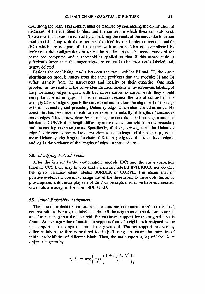
EXTRACTION OF PERCEPTUAL STRUCTURE 331
dots along the path. This conflict must be resolved by considering the distribution of distances of the identified borders and the context in which these conflicts exist. Therefore, the curves are refined by considering the result of the curve identification module (CI) along with those borders identifled by the border correction module (BC) which are not part of the clusters with interiors. This is accomplished by looking at the configurations in which the contkt arises. The aspect ratios of the edges are computed and a threshold is applied so that if this aspect ratio is sufficiently large, then the longer edges are assumed to be erroneously labeled and, hence, deleted.
Besides the conflicting results between the two modules BI and CI, the curve identification module suffers from the same problems that the modules II and BI suffer, namely from the narrowness and locality of their expertise. One such problem in the results of the curve identification module is the erroneous labeling of long Delaunay edges aligned with but across curves as curves while they should really be labeled as gaps. This error occurs because the lateral context of the wrongly labeled edge supports the curve label and so does the alignment of the edge with its succeeding and preceding Delaunay edges which also labeled as curve. No constraint has been used to enforce the expected similarity of lengths of successive curve edges. This is now done by enforcing the condition that an edge cannot be labeled as CURVE if its length differs by more than a threshold from the preceding and succeeding curve segments. Specifically, if dj > pd + no, then the Delaunay edge i is deleted as part of the curve. Here di is the length of the edge i, pd is the mean Delaunay edge length of a chain of Delaunay edges on the two sides of edge i, and uj is the variance of the lengths of edges in those chains.
5.8. Identifying Isolated Points
After the interior border combination (module IBC) and the curve correction (module CC), there may be dots that are neither labeled INTERIOR, nor do they belong to Delaunay edges labeled BORDER or CURVE. This means that no positive evidence is present to assign any of the three labels to these dots. Since, by presumption, a dot must play one of the four perceptual roles we have enumerated, such dots are assigned the label ISOLATED.
5.9. Initial Probability Assignments
The initial probability vectors for the dots are computed based on the local compatibilities. For a given label at a dot, all the neighbors of the dot are scanned and for each neighbor the label with the maximum support for the original label is found. An average value of maximum supports from all neighbors is assigned as the net support of the original label at the given dot. The net support received by different labels are then normalized to the [0, l] range to obtain the estimates of initial probabilities of different labels. Thus, the net support s,(X) of label A at object i is given by
si(h) = avg mAax i i
1 + rij(X, h’)
j 2 i)
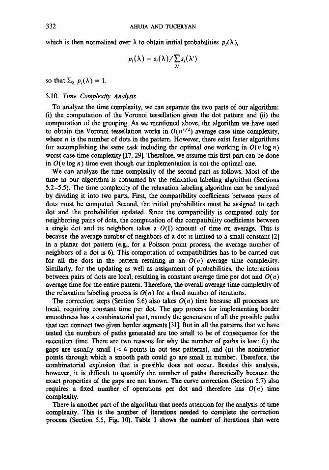
332 AHUJA AND TUCERYAN
which is then normalized over X to obtain initial probabilities p,(X),
Pi(‘) = si(h)/Csi(X’) X’
so that Ch p,(X) = 1.
5.10. Time Complexity Analysis
To analyze the time complexity, we can separate the two parts of our algorithm: (i) the computation of the Voronoi tessellation given the dot pattern and (ii) the computation of the grouping. As we mentioned above, the algorithm we have used to obtain the Voronoi tessellation works in O(n3/*) average case time complexity, where n is the number of dots in the pattern. However, there exist faster algorithms for accomplishing the same task including the optimal one working in O(n log n) worst case time complexity [17, 291. Therefore, we assume this first part can be done in O(n log n) time even though our implementation is not the optimal one.
We can analyze the time complexity of the second part as follows. Most of the time in our algorithm is consumed by the relaxation labeling algorithm (Sections 5.2-5.5). The time complexity of the relaxation labeling algorithm can be analyzed by dividing it into two parts. First, the compatibility coefficients between pairs of dots must be computed. Second, the initial probabilities must be assigned to each dot and the probabilities updated. Since the compatibility is computed only for neighboring pairs of dots, the computation of the compatibility coefficients between a single dot and its neighbors takes a O(1) amount of time on average. This is because the average number of neighbors of a dot is limited to a small constant [2] in a planar dot pattern (e.g., for a Poisson point process, the average number of neighbors of a dot is 6). This computation of compatibihties has to be carried out for all the dots in the pattern resulting in an O(n) average time complexity. Similarly, for the updating as well as assignment of probabilities, the interactions between pairs of dots are local, resulting in constant average time per dot and O(n) average time for the entire pattern. Therefore, the overall average time complexity of the relaxation labeling process is O(n) for a fixed number of iterations.
The correction steps (Section 5.6) also takes O(n) time because all processes are local, requiring constant time per dot. The gap process for implementing border smoothness has a combinatorial part, namely the generation of all the possible paths that can connect two given border segments [31]. But in all the patterns that we have tested the numbers of paths generated are too small to be of consequence for the execution time. There are two reasons for why the number of paths is low: (i) the gaps are usually small (-c 4 points in out test patterns), and (ii) the noninterior points through which a smooth path could go are small in number. Therefore, the combinatorial explosion that is possible does not occur. Besides this analysis, however, it is difficult to quantify the number of paths theoretically because the exact properties of the gaps are not known. The curve correction (Section 5.7) also requires a fixed number of operations per dot and therefore has O(n) time complexity.
There is another part of the algorithm that needs attention for the analysis of time complexity. This is the number of iterations needed to complete the correction process (Section 5.5, Fig 10). Table 1 shows the number of iterations that were
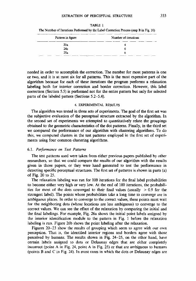
EXTRACTION OF PERCEPTUAL STRUCTURE 333
TABLE 1 The Number of Iterations Performed by the Label Correction Process (step B in Fig. 10)
Pattern in figure Number of iterations
20a 4 24a 6 25a 6
needed in order to accomplish the correction. The number for most patterns is one or two, and it is at most six for all patterns. This is the most expensive part of the algorithm because for each of these iterations the program performs a relaxation labeling both for interior correction and border correction. However, this label correction (Section 5.5) is performed not for the entire pattern but only for selected parts of the labeled pattern (Sections 5.2-5.4).
6. EXPERIMENTAL RESULTS
The algorithm was tested in three sets of experiments. The goal of the first set was the subjective evaluation of the perceptual structure extracted by the algorithm. In the second set of experiments we attempted to quantitatively relate the groupings obtained to the geometric characteristics of the dot patterns. Finally, in the third set we compared the performance of our algorithm with clustering algorithms. To do this, we computed clusters in the test patterns employed in the first set of experi- ments using four common clustering algorithms.
6.1. Performance on Test Patterns
The test patterns used were taken from either previous papers published by other researchers, so that we could compare the results of our algorithm with the results given in those papers, or they were hand generated to test the performance in detecting specific perceptual structures. The first set of patterns is shown in parts (a) of Fig. 20 to 25.
The relaxation labeling was run for 100 iterations for the final label probabilities to become either very high or very low. At the end of 100 iterations, the probabili- ties for most of the dots converged to their final values (usually > 0.9 for the strongest label). The points whose probabilities take a long time to converge are in ambiguous places. In order to converge to the correct values, these points must wait for the neighboring dots (whose locations are less ambiguous) to converge to the correct values. We can see the effect of the relaxation by comparing the initial and the final labelings. For example, Fig. 26a shows the initial point labels assigned by the interior identification module to the pattern in Fig. 1 before the relaxation labeling is run. Figure 26b shows the point labeling after the relaxation.
Figures 20-23 show the results of grouping which seem to agree with our own perception. That is, the identified interior regions and borders agree with those perceived by humans. The results shown in Fig. 24-25, on the other hand, have certain labels assigned to dots or Delaunay edges that are either completely incorrect (point A in Fig. 24, point A in Fig. 25) or that are ambiguous to humans (points B and C in Fig. 24). In most cases in which the dots or Delaunay edges are

334 AHUJA AND TUCERYAN
. :..- . . ....I . . . . :. . . . . .
.
. . :. .I: . . . . :. . . .
.:. * . . 0 . .::.. .‘. . . . . . . . . . . : . . . . . .J . . . ...’ . . . . . . . . . 0 . ..,.. . ...‘. . 0 . . . .
FIG. 20. (a) An example dot pattern. (b) The resulting identification.
. . .: . .
. . . . .‘. . . .‘. . . . . . . :: . . .
. . . . . . . . . . . . . . .
FIG. 21. (a) An example dot pattern. (b) The resulting identification.
I
: . . . . . .
. . . . . . . . . :
. . . . . . .. . .
FIG. 22. (a) An example dot pattern [33]. (b) The resulting identification.
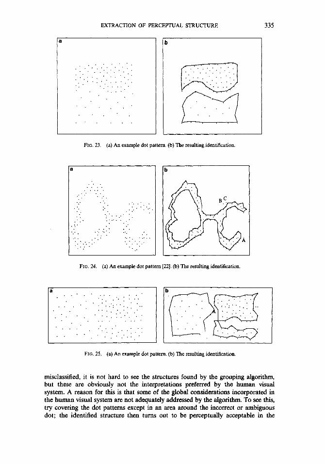
EXTRACTION OF PERCEPTUAL STRUCTURE 335
. . . ‘..
“ . . . .
. . .
, . .
. . .
. .
. . ,
‘,
. .
. .
i
. .,.. . ‘, . . . :::. a . . . . . . .:. ..,..’ . . . .a . . . . . . FIG. 23. (a) An example dot pattern. (b) The resulting identification.
. . . . . . . . . . . . . . . . . .: . . . . ‘.
. . . :. . :
* . .:. . ..’ .
: . . . . . . . . . . :
. : . : . . . . .
.: . . . . .:. . . . .
. . . . . . . . .
. . . . : .‘. . .
:: .
. . . ..
. . .
b
FIG. 24. (a) An example dot pattern [22]. (b) The resulting identification.
a . . . . . . . . :.. . . . . . . ...
. : ...... . . . : : . . . . . . . .:. . . . . .
. . . . . . . . . . . . . . . . . . .
. . . . . . ..’ . . :... . . .’ ‘. .,.. .
b
FIG. 25. (a) An example dot pattern. (b) The resulting identification.
misclassified, it is not hard to see the structures found by the grouping algorithm, but these are obviously not the interpretations preferred by the human visual system. A reason for this is that some of the global considerations incorporated in the human visual system are not adequately addressed by the algorithm. To see this, try covering the dot patterns except in an area around the incorrect or ambiguous dot; the identified structure then turns out to be perceptually acceptable in the

336 AHUJA AND TUCERYAN
a
b
FIG. 26. (a) The initial dot labels assigned by the interior identification module for the pattern in Fig. 1. The INTERIOR labeled points in this figure are those that lie inside of closed borders, similar to the results shown in Fig. 11. (b) The labels assigned to points at the end of the relaxation labeling process which are considerably different from the initial labels.
visible part of the pattern. More Gestalt constraints, beyond those we have used, are necessary to extract the correct perceptual structure in such patterns. Detection of global, texture-like structure requires even further constraints [32]. For example, the pattern in the inset Fig. 27a, in isolation, is interpreted by the algorithm to have the structure shown in Fig. 27b which is perceptually quite acceptable. But when the same structure is put in the context of the field of dot-pairs having highly correlated orientations as shown in Fig. 27, the global texture effects dominate the human visual perception and the relatively local structure extracted by the algorithm is pushed into secondary importance.
The current formulation of the border smoothness constraint also leads to errors (currently we compute a simple function of local difference between orientations of successive Delaunay edges along the border). Other, more suitable measures such as the total curvature along a border segment would improve the results in cases such as point A in Fig. 25. The errors in labeling points A, B, and C in Fig. 24 are also the result of enforcing erroneous border smoothness; the borders become smoother by excluding points A, B, and C.
Still other types of global effects involve hierarchical grouping wherein a dot’s interpretation may be determined by higher levels of groupings, i.e., those resulting from recursively formed groupings of the lowest level tokens. The final interpreta- tion thus obtained may suppress the locally evident perceptual role of the dot. As
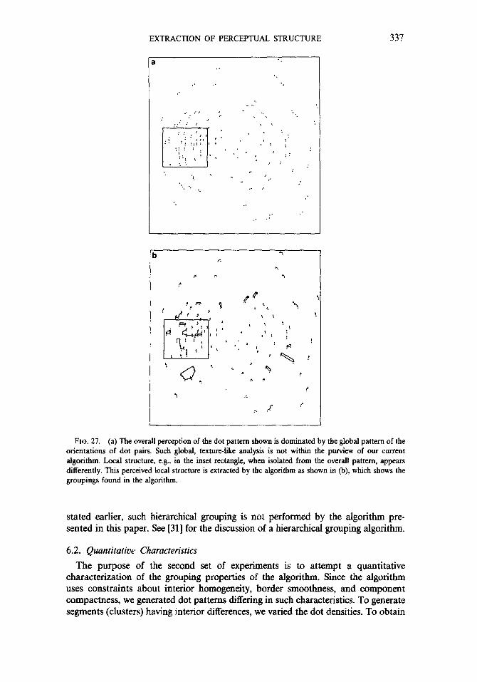
EXTRACTION OF PERCEPTUAL STRUCTURE 331
a ‘. . .
. . : . .
; , . c
..:: : : ,
:: i : : 2
: :s :: ::... . ..i
El
.
:i: : : ::.. ., ’ \ . . :
.:, c - 1. ‘. ‘. ..
. . . . . .
. : :
: :
I . . :
s :
:
. . . .
. . :
, . .’
FIG. 27. (a) The overall perception of the dot pattern shown is dominated by the global pattern of the orientations of dot pairs. Such global, texture-like analysis is not within the purview of our current algorithm. Local structure, e.g., in the inset rectangle, when isolated from the overall pattern, appears differently. This perceived local structure is extracted by the algorithm as shown in (b), which shows the groupings found in the algorithm.
stated earlier, such hierarchical grouping is not performed by the algorithm pre- sented in this paper. See [31] for the discussion of a hierarchical grouping algorithm.
6.2. Quantitative Characteristics The purpose of the second set of experiments is to attempt a quantitative
characterization of the grouping properties of the algorithm. Since the algorithm uses constraints about interior homogeneity, border smoothness, and component compactness, we generated dot patterns differing in such characteristics. To generate segments (clusters) having interior differences, we varied the dot densities. To obtain

338 AHUJA AND TUCERYAN
different degrees of border smoothness and compactness, we used segments of different shapes. Specifically, we experimented with segments shaped like a disk, square, and a star-shaped polygon. Different intersegment relationships were achieved by varying the relative locations of segments and their relative dot densities. To measure the performance we computed the ratio of the border length (i.e., the total length of Delaunay edges along the border) of the extracted and model clusters. The larger the deviation of the ratio from unity, the poorer the performance was judged to be. This performance measure, like many other quanti- tive measures may suffer from lack of perceptual validity. It may be that. a cluster actually changes significantly (perceptually) after the perturbation. If so, its per- ceived border length would change also, and it would be inappropriate to use the above ratio as a performance index of the grouping algorithm. We must be aware of this shortcoming of our performance measure in interpreting the quantitative results about the grouping characteristics of our algorithm.
Each test pattern was generated starting with a regular square grid of dots with a given interdot separation. To obtain different degrees of homogeneity in the segments, the location of each dot was perturbed by an amount Ax and Ay in the x and y directions, respectively. The values of Ax and Ay were determined by the expression vRd, where v is a parameter that controls the extent of perturbation (0 I v < l), and R is a random number between - 1 and 1, and d is the average interdot distance. The parameter v determines the extent of randomness of the dot pattern. From experiments we found that for v > 0.5 our grouping algorithm fragments the uniform pattern and starts detecting the microclusters formed by randomly perturbed dots. Since we are not concerned with detection of global, texture-like structure in this paper, all test patterns used in our experiments were generated using 0 I v < 0.5, in particular v = 0.3 and v = 0.5.
The first set of patterns we generated consists of two segments with uniform density. A circular disk of density ai was placed inside another circular region of density a1 (Fig. 28). Since we knew exactly where the true border lies separating the two regions, we could measure the performance of the grouping algorithm quantita- tively as the ratio of the detected border length to the true border length. We varied the ratio of the two densities ai and a*, and computed percentage of the true border detected by the algorithm for various values of al/az. This entire experiment was repeated for five sets of patterns generated using different seeds for the random number generator, and the results were averaged for each density ratio. The results are shown in Figs. 29 and 30. As expected the detection of the border separating the two regions deteriorates as the dot densities in the two regions approach each other. For very low ratios the detected borders are usually microedges corresponding to random subsegments. The breakdown point for detection is around al/az = 5.
The next set of patterns was generated by the same process as above, except that the shape of the central region was made a square (Fig. 28). In this case it was expected that because of border smoothness constraint used by the algorithm, comers of the square would not be detected well. Again, five sets of patterns were generated and their results averaged. The results are given in Figs. 29 and 31. The breakdown point for detection in this case is around a density ratio of 6, reflecting a poorer performance relative to the previous case of disks.
In the third set of patterns the central region was star shaped with four points, which results in the region having a total of eight comers four of which are convex

EXTRACMON OF PERCEPTUAL STRUCTURE 339
B C
FIG. 28. Examp$s of test patterns used for quantitive analysis (V = 0.3). Each now corresponds to a different shape central region: top-circle, middle-square, and bottom-star. Each column corresponds to a different density ratio a1/a2. Column (A) shows a large ratio, (Y~/oL~ = 26. Column (B) shows a comparable density case, OI,/OL~ = 1.21. Column (C) shows aI/uz values near the breakpoint of 4.
and four are concave (Fig. 28). The observations were again made on five sample patterns and the results averaged. The expectation in this case was that the performance of the algorithm would suffer even more because the number of corners in the border to be detected increased, and therefore the border smoothness constraint would miss more points along the border. For the low values of ar,/~y, (below the breakpoint value of six) we see that in some cases the algorithm performs better for the star-shaped region than the square shape region. In this range of ratios and v values, however, the perceptual differences due to differences in region

AHUJA AND TUCERYAN
C
FIG. 29. The results obtained from the patterns in Fig. 28 shown in the same format as Fig. 28.
densities become very weak. The random perturbations in the locations of dots create accidental gaps in the uniform region. The borders detected are those of the accidentally created, although perceptually valid structure, which does not match the original noise-free structure (e.g., see Fig. 29, column B). Thus, comparison of the algorithm performance in this range for various shapes becomes very unreliable. The results are given in Figs. 29 and 32.
To compare the performance of the algorithm on the three patterns above, Fig. 33 shows the results on the same set of axes. As expected, within the more reliable range of density ratios the circle within a circle is segmented best and the star within a circle is segmented the worst.

FXTRACTION OF PERCEPTUAL STRUCTURE 341
borders detected
I I I I I I 0 5 10 15 20 25
al 4
FIG. 30. The performance of the grouping algorithm for a circular region with dot density or within a circular region with density a,. The solid line represents the percentage of the true border detected by the algorithm for perturbation Y 0 0.3 and the dashed line for Y = 0.5.
To examine the effect of the separation of clusters on the performance of the algorithm, we used two circularly shaped uniform clusters placed at various dis- tances. The separation between the clusters was measured as the minimum distance between their centers normalized by the average of the interdot distances in the two clusters. The grouping performance was again measured as the percentage of the true border dots detected along the crack between two clusters. The crack between two clusters consists of adjacent points across the two borders, i.e., those points on the border of the first cluster which have at least one Voronoi neighbor that belongs to the second cluster, and vice versa. In other words, the performance measure is based on only those points whose interpretation is a!Tected by the separation of the two clusters. The results give us some idea about the interaction between the constraints of interior homogeneity and border smoothness. It is expected that two clusters with similar dot densities would be segmented even for a separation of less than average interdot distance because of the border smoothness constraint; if not
I I I I I 0 5 10 15 20 25
ai Ia2
FIG. 31. The performance of the grouping algorithm for a square region with dot density a, within a circular region with density 0s. The solid line represents the percentage of the true border defected by the algorithm for perturbation v = 0.3 and the dashed fine for Y = 0.5.

342 AHUJA AND TUCERYAN
Percent of borders detected
40
I I I I I I
0 5 10 15 20 25 a~ Ia2
FIG. 32. The performance of the grouping algorithm for a star shaped region with dot density aI within a circular region with density as. The solid line represents the percentage of the true border detected by the algorithm for perturbation v = 0.3 and the dashed line for v = 0.5.
for border smoothness such clusters would be detected as a single dumbbell-shaped blob. The results confirm this. Figure 34 shows that the true borders are identified completely (i.e., 100%) for minimum gap distance of 90% of the average interdot distance. For smaller gaps, the algorithm does not completely separate the two clusters; visually also, in such cases, the pattern appears to be a cluster with a neck. As also expected, the performance degrades with larger amounts of perturbation.
Finally, to examine the effect of interior homogeneity of clusters along with cluster separation, we generated gaussian clusters at various separations. The dot density in the interior of a gaussian cluster depended upon the radial distance from the cluster center according to the formula density = D0e-r2/“2. Here D, is the density of the cluster at the center, r is the radial distance from the center, and (I is the standard deviation. The clusters were again generated as regular patterns with the above density profile and then perturbed by various amounts. The amount of perturbation was given by the formula vRd as above, where v is the control
r
Percent of 60
borders detected 40
FIG. 33. The performance of the grouping algorithm for the three different shapes shown. Ah three are compared for a perturbation value of v = 0.3. The solid line represents the circle within a circle pattern. the dashed line square within a circle, and the dotted line star within a circle.
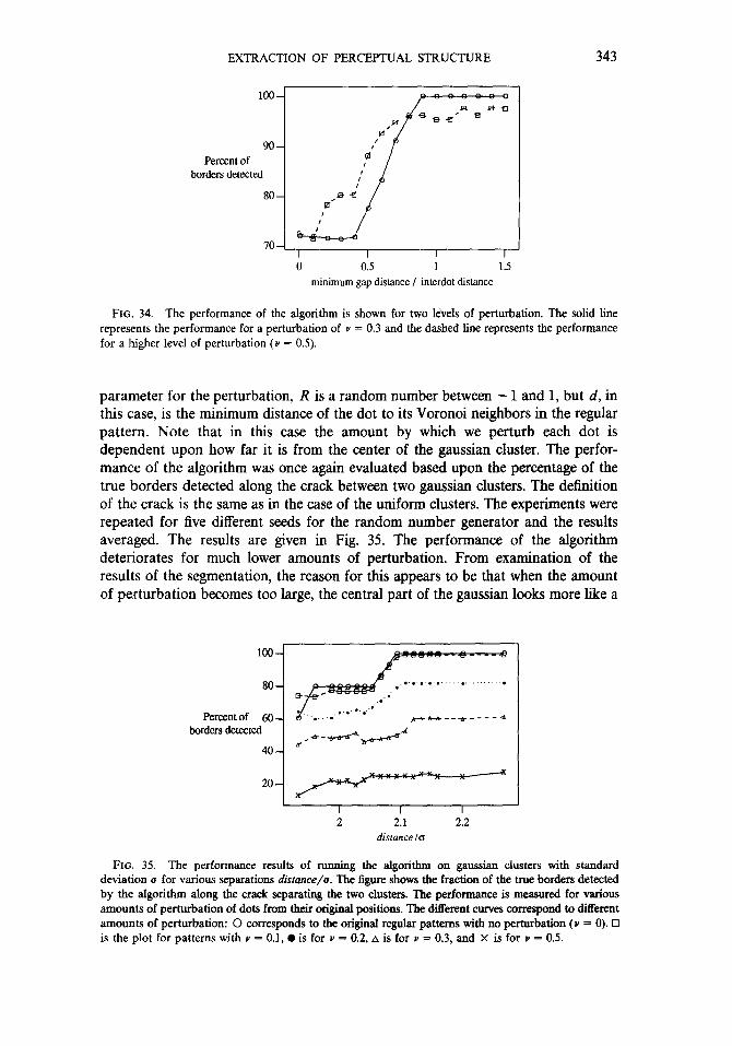
EXTRACTION OF PERCEPTUAL STRUCTURE 343
90 Percent of
borders detected
80
0 0.5 1 1.5 minimum gap distance / interdot distance
FIG. 34. The performance of the algorithm is shown for two levels of perturbation. The solid line represents the performance for a perturbation of Y = 0.3 and the dashed line represents the performance for a higher level of perturbation (Y = 0.5).
parameter for the perturbation, R is a random number between - 1 and 1, but d, in this case, is the minimum distance of the dot to its Voronoi neighbors in the regular pattern. Note that in this case the amount by which we perturb each dot is dependent upon how far it is from the center of the gaussian cluster. The perfor- mance of the algorithm was once again evaluated based upon the percentage of the true borders detected along the crack between two gaussian clusters. The definition of the crack is the same as in the case of the uniform clusters. The experiments were repeated for five different seeds for the random number generator and the results averaged. The results are given in Fig. 35. The performance of the algorithm deteriorates for much lower amounts of perturbation. From examination of the results of the segmentation, the reason for this appears to be that when the amount of perturbation becomes too large, the central part of the gaussian looks more like a
100
80
Percentof fj0 horders detected .*-#*,&+d d
I I I I 2 2.1 2.2
distance lo
FIG. 35. The performance results of running the algorithm on gaussian clusters with standard deviation u for various separations distance/u. The figure shows the fraction of the true borders detected by the algorithm along the crack separating the two clusters. The performance is measured for various amounts of perturbation of dots from their original positions. The different curves correspond to different amounts of perturbation: 0 corresponds to the original regular patterns with no perturbation (V = 0). q is the plot for patterns with Y = 0.1, 0 is for Y = 0.2, A is for Y = 0.3, and X is for Y = 0.5.

344 AHUJA AND TUCERYAN
uniform region, and the less dense outer part of the gaussian appears to consist of isolated background noise points. This results in parts of the true border being missed for large perturbations. When the perturbation becomes even larger, we see once more the texture-like effects and start detecting micro-edges.
In each case, our experimental results (Figs. 30-33) show an interesting phe- nomenon: as (Y~/(Y* increases, the performance of border detection for larger perturbation values relative to smaller perturbation values changes. For low OL~/OL~ values, patterns with higher perturbation (V = 0.5) lead to better border detection than patterns with lower perturbation (V = 0.3). For large (Y~/(Y* values, v = 0.3 leads to better border detection. We observe the same effect in the experiments on the effect of cluster separation on the performance of the segmentation algorithm (Figs. 34, 35). This can be explained by the fact that the regular pattern which underlies our test patterns is defined on a square grid. This results in the generation
b
FIG. 36. The clusters detected in the dot pattern in Fig. 1 by (a) single linkage hierarchical clustering algorithm, (b) complete linkage hierarchical clustering algorithm, (c) FORGY (k-means) square error clustering algorithm, and (d) CLUSTER (k-means) square error clustering algorithm. The corresponding results obtained by our algorithm are shown in Fig. 16.
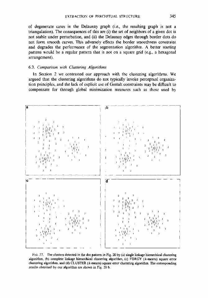
EXTRACTION OF PERCEPTUAL STRUCTURE 345
of degenerate cases in the Delaunay graph (i.e., the resulting graph is not a triangulation). The consequences of this are (i) the set of neighbors of a given dot is not stable under perturbation, and (ii) the Delaunay edges through border dots do not form smooth curves. This adversely effects the border smoothness constraint and degrades the performance of the segmentation algorithm. A better starting pattern would be a regular pattern that is not on a square grid (e.g., a hexagonal arrangement).
6.3. Comparison with Clustering Algorithms
In Section 2 we contrasted our approach with the clustering algorithms. We argued that the clustering algorithms do not typically invoke perceptual organiza- tion principles, and the lack of explicit use of Gestalt constraints may be difficult to compensate for through global minimization measures such as those used by
2
1 2
2 2 = 2
2 :12= 2
= 2 2 222
22222 =
2 1
2 2 = 2
2 2
2 = 2 2 2
= 2
===2 2 2 22 22
9 22222 2
2 :’ 2 = 2
2 3
2
2
2
FIG. 37. The clusters detected in the dot pattern in Fig. 20 by (a) single linkage hierarchical clustering algorithm, (b) complete linkage hierarchical clustering algorithm, (c) FORGY (k-means) square error clustering algorithm, and (d) CLUSTER (k-means) square error clustering algorithm. The corresponding results obtained by our algorithm are shown in Fig. 20 b.

346 AHUJA AND TUCERYAN
clustering algorithms. Often the implementation of global optimality is computa- tionally complex and heuristics are used. In this section we show the results of some clustering algorithms on dot patterns for which we have already shown the results of our approach. Following are four clustering algorithms we used for this purpose (a description and a discussion of each of these algorithms can be found in [15]).
(a) Single link hierarchical clustering. This algorithm constructs a hierarchical nesting of partitions. Each partition is given by a threshold graph which is a subgraph of the complete graph defined by the dot pattern. A threshold graph for a threshold T is obtained by deleting all edges connecting points having similarity (according to some metric) measure lower than T. An increasing value of T leads to deeper nesting within the hierarchy. For any given threshold, all candidate sub- graphs of the threshold graph are said to define clusters. The algorithm requires the
FIG. 38. The clusters detected in the dot pattern in Fig. 21 by (a) single linkage hierarchical clustering algorithm, (b) complete linkage hierarchical clustering algorithm, (c) FORGY (k-means) square error clustering algorithm, and (d) CLUSTER (k-means) square error clustering algorithm. The corresponding results obtained by our algorithm are shown in Fig. 21 b.

EXTRACTION OF PERCEPTUAL STRUCTURE 347
desired number of clusters as input parameter. It then decreases the thresholds until the desired number of clusters is found.
(b) Complete fink hierarchical clustering. This algorithm is similar to (a), except that each subcluster must be a clique in the threshold graph.
(c) FORGY. This is a k-means partitional clustering algorithm that is based on minimizing a squared error criterion. It uses k initial seeds to form the partitions and iteratively corrects the partition by reassigning the dots to clusters in order to reduce the square error. A number of parameters have to be specified including the number of clusters and the initial seed points.
(d) CLUSTER. This is also a k-means partitional clustering algorithm similar to FORGY. It generates a sequence of clusterings having 1,2,, . . . , k clusters instead of one clustering. It uses different heuristics to estimate the minimum square error partition than FORGY. It requires fewer input parameters than FORGY. There-
y---T b 2
c I
I ’
i 3 1
&3 2 3 3
3 3 22 2 2
2
22 3 3’
2 ?
3 j2 2 22
2 22 22 22
33 2 2 3
2 2 2
2 2
2
2 2
22 2
2 2 2 22 3 3 2 2 33
2 2
3 3
1 I 333 ?3 1
’ I 33
3 33 3
33 I ’ I
3
I 1 I 3 33
’ ’ 33
I I ,3 33 3
I
2 2 2
2 2
2 22 2
2? 2 22 I 1 2 2 ‘1 I
2 2
2 2 I’, ‘1 3 ’ 3 1, 1 1’ 3 3 3
3 33 3 ‘3 33 ?‘,]I
i
3
, ‘I I
I i
3 3 ’
3
3 3
FIG. 39. The clusters in the dot pattern in Fig. 22 by (a) single linkage hierarchical clustering algorithm, (b) complete linkage hierarchical clustering algorithm, (c) FORGY (k-means) square error clustering algorithm, and (d) CLUSTER (k-means) square error clustering algorithm. The corresponding results obtained by our algorithm are shown in Fig. 22 b.

348 AHUJA AND TUCERYAN
3 3 3 3 3
33 3 3 3 3 3
3 3 3 3
3
3 3 3 33 3 3
3
1 ’ I 1
1 II
I 1
I 1
1 ’
I 1 I 1
I I
2
2 2
3
2 2 2 2
2 2 2
2 3 3
3 7
2 3 2
2
3 3 3
3 3 3
3 3 3
3
3 3
3 3
3 3
3 3 3
3 3 3 3
3
222
2
2 22
2 2
2 2
I I I 1
FIG. 40. The clusters detected in the dot pattern in Fig. 25 by (a) single linkage hierarchical clustering algorithm, (b) complete linkage hierarchical clustering algorithm, (c) FORGY (k-means) square error clustering algorithm, and (d) CLUSTER, (k-means) square error clustering algorithm. The corresponding results obtained by our algorithm are shown in Fig. 25 b.
fore, the final clustering obtained by CLUSTER is, in general, different from that derived by FORGY, although both, in general, give partitions having higher than optimal value of the square error. The user has to specify a smaller number of parameters.
Each of these algorithms was run on the dot patterns in Figs. 1,20, 21,22, and 25. In each case, the algorithm was applied with the correct number of clusters. For the FORGY algorithm, the k cluster centers were generated randomly. The seed for the random number generator was supplied externally and an error threshold was used to decide when to create a new cluster. The use of this threshold is typical of decision making steps in these and other clustering algorithms; for example, to determine when to merge clusters, how often to compute cluster means, and how to reassign points to clusters. No such parameters are required by our algorithm, which, of course, has more basic, built-in, general purpose thresholds as discussed in

EXTRACTION OF PERCEPTUAL STRUCTURE 349
Section 4 and Appendix A. The outputs of the clustering algorithms are shown in Figs. 36-40; each figure shows the outputs of the four algorithms on the same dot pattern. Unlike the results of our algorithm, no borders are shown here because the clustering algorithms identify only the set of dots belonging to a cluster without assigning any structural roles to them. With few exceptions, the detected clusters are in disagreement with perceptual clusters. It is clear that the optimality measures that the clustering algorithms use group the dots in unacceptable ways. In general, compact well-separated clusters are more likely to be successfully extracted than curvilinear clusters, or two clusters, one within the other (e.g., Fig. 22).
7. SUMMARY
The problem of dot pattern analysis is of importance to computer vision because images can often be transformed into labeled dot patterns, where the dots represent image tokens (such as blobs or edge segments). Any analysis that involves the tokens can then be performed on the dot pattern. A simple example of this is image segmentation into perceptual clusters of tokens which are based only on their relative locations. Detection of barren land, dense vegetation, or road networks within aerial images are some problems that fall in the above category, assuming of course that operators are available that would respond to points in the above regions with spatial regularity, so as to transform the regions into token clusters. To identify the different clusters as well as their shapes is the problem we have discussed in this paper. The performance of a grouping algorithm is evaluated by the extent to which the detected groupings agree with human judgment; we have no objective measure of evaluating the results.
The key feature of the problem is that perception of dot clusters is the result of grouping together of subsets of dots having appropriate relative positions, since the dots do not differ in characteristics such as color or shape. An immediate question one faces in developing a grouping algorithm is how to express the mutual compatibility of dot positions for grouping. In the large body of work available on clustering, this question has been mainly answered in the terms of interdot dis- tances; specifically, clusters are defined so as to minimize some objective function of within cluster and cross cluster dot locations. The objective function is many times defined in ternis of distances to “neighbors” which are considered to be the dots tha.t are: within a certain threshold distance, or the k nearest ones (for some specified k), or those connected by the edges of a predefined graph (e.g., minimum spanning tree). The quality of the final grouping then is bound by the perceptual validity of the objective function and the definition of a neighbor.
The first point of this paper is that it is important to characterize spatial structure in the vicinity of a dot and then group dots based on the similarity of their local spatial structures. We have argued that “neighborhoods” instead of neighbors should be used to better capture the perceptual notion of a dot’s surrounding structure. Thus, a dot should be described by a two-dimensional region instead of a set of distances to other dots. The Voronoi neighborhood that we have used for this purpose is appealing because of its construction.
The second point of the paper is that detection of the perceptual structure should be done through detection of the components of the structure. This has two aspects, First, the clusters are “assembled” from the border points, interior points, curves, and isolated points which are themselves detected by different (but cooperating)

350 AHUJA AND TUCERYAN
procedures. This is in contrast to a partitioning of the dot pattern to achieve some global optimization as done in many clustering algorithms. Second, the need for constructing the clusters from components also means that the detection process should retain the planar framework of the problem and the simplicity of the nature of interaction among perceptual components. Neither of these aspects is novel to our work; Zucker and Hummel describe a similar approach [44]. In both cases a probabilistic relaxation process achieves constraint propagation. However, our approach differs in some significant ways. The first of these is an immediate consequence of our use of the Voronoi neighborhoods. We can state how the different components of perceptual structure can be recognized from intrinsic geometric properties of the Voronoi neighborhoods. Zucker and Hummel get these estimates from a priori defined numerical constraints on properties such as inter- point distances. Due to the power of the Voronoi neighborhood representation, we have better initial estimates of the probabilities of the perceptual roles different dots play. Further, the refinement of these probabilities through relaxation may be more efficient since the Voronoi neighbors defined by the Delaunay graph better meet the perceptual notion of neighbors than other definitions including the k-nearest neighbors used by Zucker and Hummel. For example, the Delaunay graph is planar, the corresponding neighbors are symmetric, and grouping proceeds much in the way of standard graph theoretic clustering algorithms while using similarity measures on the properties of Voronoi neighborhoods. This single step (of using Voronoi neighborhoods and neighbors) actually takes us a long way towards minimizing the use of critical, pattern-sensitive thresholds. The second difference is that we also use curves as a component of perceptual structure, whereas Zucker and Hummel use only interior, border, and isolated points. We have argued that the set of four labels we have used is complete.
The third point of the paper is that the local perceptual structure can be suppressed by nonlocal constraints. That is, the structure that we may perceive when we cover up the dot pattern except in a small window around a dot could be different when the same window is seen in the context of the entire pattern. The nonlocal constraints that must be taken into account may have different scopes: for example, the local interpretation of a dot may become INTERIOR from the locally perceived BORDER because the new interpretation leads to a smoother border, or a more compact component, or a smoother (optical) flow, or a more uniform texture. This continuum of nonlocal constraints with increasingly global scope actually reaches the realm of semantics in the general problem of vision. Enumeration of these constraints even for the relatively low level constraints is not available. However, integration of such constraints with the local perceptual interpretation is a key to the development of general perceptual clustering algorithms. A significant part of the paper is that we attempted to integrate three of the constraints namely local structure, border smoothness, and component compactness.
An important dimension of the perceptual clustering problem is the recursive nature of it. The groupings of dots may themselves form tokens to be further grouped. An obvious difference between the grouping of dots in the dot pattern, and recursive grouping among cluster tokens is that all tokens beyond the level of dots are nonpoint objects and unlike dots possess properties such as shape, orientation, and size. The recursive grouping of tokens thus may depend not only on the positions of the tokens but also on the other properties; the nature of the compo-
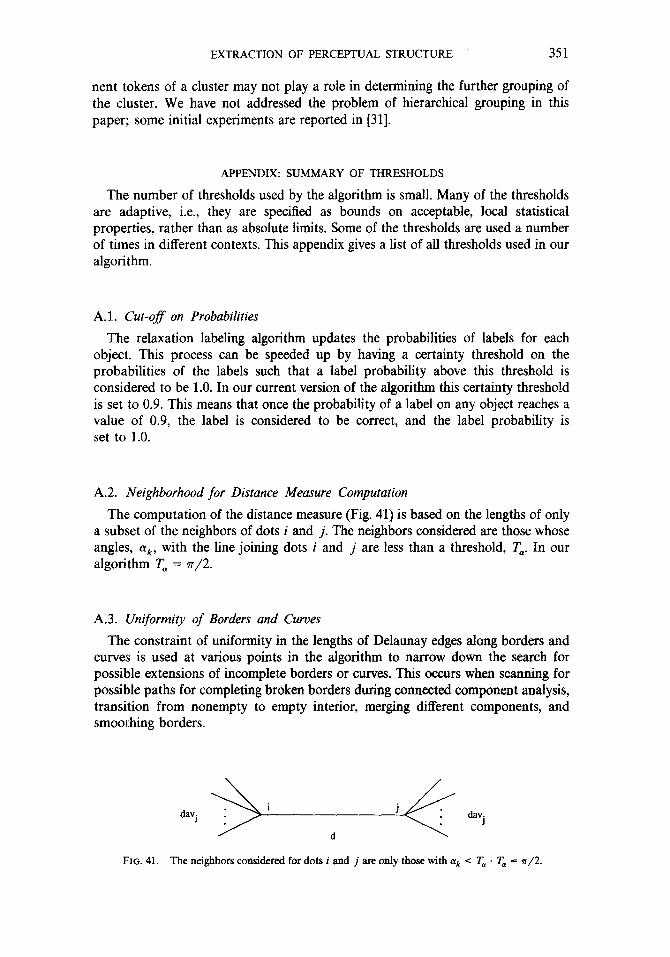
EXTRACTION OF PERCEPTUAL STRUCTURE 351
nent tokens of a cluster may not play a role in determining the further grouping of the cluster. We have not addressed the problem of hierarchical grouping in this paper; some initial experiments are reported in [31].
APPENDIX: SUMMARY OF THRESHOLDS
The number of thresholds used by the algorithm is small. Many of the thresholds are adaptive, i.e., they are specified as bounds on acceptable, local statistical properties, rather than as absolute limits. Some of the thresholds are used a number of times in different contexts. This appendix gives a list of all thresholds used in our algorithm.
A.1. Cut-off on Probabilities
The relaxation labeling algorithm updates the probabilities of labels for each object. This process can be speeded up by having a certainty threshold on the probabilities of the labels such that a label probability above this threshold is considered to be 1.0. In our current version of the algorithm this certainty threshold is set to 0.9. This means that once the probability of a label on any object reaches a value of 0.9, the label is considered to be correct, and the label probability is set to 1.0.
A.2. Neighborhood for Distance Measure Computation
The computation of the distance measure (Fig. 41) is based on the lengths of only a subset of the neighbors of dots i and j. The neighbors considered are those whose angles, q, with the line joining dots i and j are less than a threshold, T,. In our algorithm T, = n/2.
A.3. Uniformity of Borders and Curves
The constraint of uniformity in the lengths of Delaunay edges along borders and curves is used at various points in the algorithm to narrow down the search for possible extensions of incomplete borders or curves. This occurs when scanning for possible paths for completing broken borders during connected component analysis, transition from nonempty to empty interior, merging different components, and smoothing borders.
FIG. 41. The neighbors considered for dots i and j are only those with ak c: T, . T, = s/2.

352 AHUJA AND TUCERYAN
J
FIG. 42. The neighbors (e.g., j) of the endpoint i are searched for possible extension of the border segment terminating at i. If the length of edge g is much larger than the average edge length along the segment, then the point j is not considered for possible extension. There is also an upper limit to the angle a for point j to be considered a neighbor.
Given a border segment of n points (connected by n - 1 Delaunay edges), the border uniformity measure is computed as follows. First we compute the average distance measure auerage-distance of the Delaunay edges in the border segment.
average-distance = Wi) - dnmx
(n-l) ’
where di’s are the lengths of the Delaunay edges in the border segment, and d,, is the length of the longest edge. Now, using this measure we compute the uniformity measure, unif,
unif = average-distance
d ’ max
The uniformity measure will be very close to 1.0 when the border segment consists of very regularly spaced dots. It will be very close to 0.0 if there is a very long edge in the border segment.
In the search for a Delaunay edge to extend the border segment, the neighbors of the endpoint under consideration are scanned (Fig. 42). Using a neighbor to extend the border segment may change the uniformity measure of the extended segment. A
FIG. 43. The search for the Delaunay edges that merge components. The neighbors (j) of the high curvature point i are searched for possible merging of the components to which i and j belong.
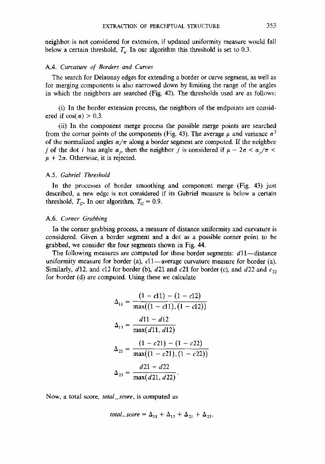
EXTRACTION OF PERCEPTUAL STRUCTURE 353
neighbor is not considered for extension, if updated uniformity measure would fall below a certain threshold, T,. In our algorithm this threshold is set to 0.3.
A.4 Curvature of Borders and Curves
The search for Delaunay edges for extending a border or curve segment, as well as for merging components is also narrowed down by limiting the range of the angles in which the neighbors are searched (Fig. 42). The thresholds used are as follows:
(i) In the border extension process, the neighbors of the endpoints are consid- ered if cos(a) > 0.3.
(ii) In the component merge process the possible merge points are searched from the corner points of the components (Fig. 43). The average p and variance a* of the normalized angles OL/~T along a border segment are computed. If the neighbor j of the dot i has angle a!, then the neighbor j is considered if p - 2a < 01,/q < p + 20. Otherwise, it is rejected.
AS. Gabriel Threshold
In the processes of border smoothing and component merge (Fig. 43) just described, a new edge is not considered if its Gabriel measure is below a certain threshold, T,. In our algorithm, T, = 0.9.
A.6. Corner Grabbing
In the corner grabbing process, a measure of distance uniformity and curvature is considered. Given a border segment and a dot as a possible corner point to be grabbed, we consider the four segments shown in Fig. 44.
The following measures are computed for these border segments: dll-distance uniformity measure for border (a), cll-average curvature measure for border (a). Similarly, d12, and cl2 for border (b),‘d21 and ~21 for border (c), and d22 and cZ2 for border (d) are computed. Using these we calculate
(1 - cll) - (1 - c12)
‘11 = max((1 - cll),(l - ~12))
dll - d12 43 = max( dll, d12)
(1 - c21) - (1 - c22)
A21 = max((1 - c21),(1 - ~22))
d21 - d22 A23 = max( d21, d22) ’
Now, a total score, total-score, is computed as
total-score = AI1 + AI3 + A21 + A23.
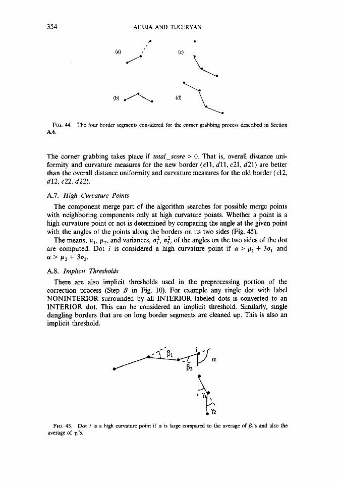
354 AHUJA AND TUCERYAN
FIG. 44. The four border segments considered for the comer grabbing process described in Section A.6.
The corner grabbing takes place if total-score > 0. That is, overall distance uni- formity and curvature measures for the new border (~11, dll, ~21, d21) are better than the overall distance uniformity and curvature measures for the old border (~12, d12, ~22, d22).
A.7. High Curvature Points
The component merge part of the algorithm searches for possible merge points with neighboring components only at high curvature points. Whether a point is a high curvature point or not is determined by comparing the angle at the given point with the angles of the points along the borders on its two sides (Fig. 45).
The means, pi, pLz, and variances, ut, ,‘, (I of the angles on the two sides of the dot are computed. Dot i is considered a high curvature point if (Y > pi + 30, and a > p* + 30,.
A.8. Implicit Thresholds
There are also implicit thresholds used in the preprocessing portion of the correction process (Step B in Fig. 10). For example any single dot with label NONINTERIOR surrounded by all INTERIOR labeled dots is converted to an INTERIOR dot. This can be considered an implicit threshold. Similarly, single dangling borders that are on long border segments are cleaned up. This is also an implicit threshold.
FIG. 45. Dot i is a high curvature point if a is large compared to the average of &‘s and also the average of y, ‘s.

EXTRACTION OF PERCEPTUAL STRUCTURE 355
ACKNOWLEDGMENTS
We are indebted to the anonymous reviewers for their very helpful comments on the manuscript.
REFERENCES 1. N. Ahuja, “Dot Pattern Processing Using Voronoi Neighborhoods,” IEEE Trans. Pattern Analysis.
Mach. Intell. PAMI-4, No. 3, 1982, 336-343. 2. N. Ahuja and B. Schachter, Pattern Models, Wiley, New York, 1983. 3. E. Borjesson and C. von Hofsten, Spatial determinants of depth perception in two-dot motion
patterns, Percept. Psychophys. 11, No. 4, 1972, 263-268. 4. E. Borjesson and C. von Hofsten, Visual perception of motion in depth: Application of a vector
model to three-dot motion patterns, Percept. Psychophys. 13, No. 2, 1973, 169-179. 5. C. R. Brice and C. L. Fennema, Scene analysis using regions, Arttf. Intell. 1, 1970, 205-226. 6. C. K. Chow and T. Kaneko, Automatic boundary detection of the left ventricle from cineangiograms,
Comput. Biomed. Res. 5, 1972, 388-510. 7. R. Dubes and A. K. Jain, Clustering techniques: The user’s dilemma, Pattern Recognit. 8, 1976,
247-260. 8. R. 0. Duda and P. E. Hart, Pattern Classification and Scene Analysis, Wiley, New York, 1973. 9. J. Fairfield, Segmenting dot patterns by Voronoi diagram concavity, IEEE Trans. Pattern Anal.
Much. htell. PAMI-5, 1983, 104-110. 10. J. Fairfield, Segmenting blobs into subregions, IEEE Trans. Systems Man Cybernet. SMC-13, 1983,
363-384. 11. L. Glass, Moire effect from random dots, Nature 223, 1969, 578-580. 12. L. Glass and R. Perez, Perception of random dot interference patterns, Nature 246, 1973, 360-362. 13. L. Glass and E. Switkes, Pattern recognition in humans: Correlations which cannot be perceived,
Perception 5. 1976, 67-72. 14. J. N. Gupta and P. A. Wintz, A boundary finding algorithm and its applications, IEEE Trans.
Circuits und Systems CAS-22, 1975, 351-362. 15. A. K. Jain and R. C. Dubes, Algorithms for Clustering Data, Prentice-Hall, Englewood Cliffs, NJ,
1988. 16. K. KotBca, Principles of Gestalt Psychology, Harcourt Brace, New York, 1935. 17. D. T. Lee, Proximity and Reachability in the Plane, Ph.D. dissertation, CSL Report ACT-15
University of Illinois at Urbana-Champaign, 1978. 18. M. D. Levine and S. I. Shaheen, A modular computer vision system for picture segmentation and
interpretation, IEEE Trans. Pattern Anal. Mach. Intell. PAMI-3, 1981, 540-556. 19. D. G. Lowe, Perceptual Organization and Visual Recognition, Ph.D. thesis, Stanford University, 1984. 20. D. Marr, Vision, Freeman, San Francisco, 1982. 21. J. L. Meurle and D. C. Allen, Experimental evaluation of techniques for automatic segmentation of
objects in a complex scene, in Pictorial Pattern Recognition, (G. C. Chang, R. S. Ledley, D. K. Pollock, and A. Rosenfield, Eds.), pp. 3-13, Thompson, Washington, DC, 1968.
22. J. F. O’Callaghan. Computing the perceptual boundaries of dot patterns, Comput. Graphics Image Processing, 3, 1974. 141-162.
23. J. F. O’Callaghan, An alternative definition for neighborhood of a point, IEEE Trans. Comput. C-24, 1975. 1121-1125.
24. R. Ohlander, K. Price, and D. R. Reddy, Picture segmentation using a recursive region splitting method, Comput. Graphics Image Process. 8, 1978, 313-333.
25. E. A. Patrick and L. Shen, Interactive use of problem knowledge for clustering and decision making, IEEE Trans. Comput. C-20, 1971, 216-222.
26. J. S. M. Prewitt and M. L. Mendlesohn, The analysis of cell images, Ann. New York Acad. Sci., Vol. 128, pp. 1035-1053, New York Acad. Sci., New York, 1966.
27. I. Rock, The Logic’of Perception, MIT Press, Cambridge, MA, 1983. 28. A. Rosenfield, R. Hummel, and S. Zucker, Scene labeling by relaxation operations, IEEE Trans.
Systems Mutt Qbernet. SMC-6, 1976, 420-433. 29. M. I. Shames and D. Hoey, Closest-point problems, in Proceedings, 16th Annual Symp. on Founda-
tions of Computer Science, October I975, pp. 131-162. 30. 6. T. Toussaint, The relative neighborhood graph of a finite planar set, Pattern Recognit., 12, 1980,
:261-268.

356 AHUJA AND TUCERYAN
31. M. Tuceryan and N. Ahuja, Extracting Perceptual Structure in Dot Patterns: An Integrated Approach, Technical Report IULU-ENG-87-2206, Coordinated Science Laboratory, University of Illinois at Urbana-Champaign, January 1987.
32. M. Tuceryan, A. K. Jain, and Y. Lee, Texture segmentation using Voronoi polygons, in Proceedings, IEEE Conference on Computer Vision and Pattern Recognition, Ann Arbor, MI, 1988, pp. 94-99.
33. R. B. Urquhart, Graph theoretical clustering based on limited neighborhood sets, Pattern Recognit. 15, No. 3, 1982,173-187.
34. W. R. Uttal, L. M. Bunnell, and S. Corwin, On the detectability of straight lines in the visual noise: An extension of French’s paradigm into the millisecond domain, Percept. Psychophys. 8, No. 6,1970, 385-388.
35. F. R. D. Velasco, A method for the analysis of Gaussian-like clusters, Pattern Recognit. 12, 1980, 381-393.
36, R. Vistnes, Detecting structure in random-dot patterns, in Proceedings Workshop on Image Under- stand&, DA RPA, Dec. 1985, pp. 350-362.
37. G. Voronoi, Nouvelles applications des parameters continus a la theorie des formes quadratiques. Deuxieme memoire: Recherches sur les parallelloedres primitifs., J. Reine Angew. Math. 134, 1908, 198-287.
38. M. Wertheimer, Laws of organization in perceptual forms, in A Source Book of Gestalt Psychology (W. D. Ellis, Ed.), pp. 71-88, Harcourt Brace, New York, 1938.
39. A. P. Witkin and J. M. Tenenbaum, On the role of structure in vision, in Human and Machine Vision (Jacob Beck, Barbara Hope, and Azriel Rosenfeld, Eds.), pp. 481-543, Academic Press, New York, 1983.
40, M. Yachida and S. Tsuji, Application of color information to visual perception, Pattern Recognit. 3, 1971, 307-323.
41. C. T. Zahn, Graph theoretical methods for detecting and describing Gestalt clusters, IEEE Trans. Comput. C-20,1971,68-86.
42. S. W. Zucker, Region growing: Childhood and adolescence, Comput. Graphics Image Process. 5, 1976, 382-399.
43. S. W. Zucker, Vertical and horizontal processes in low level vision, in Computer Vision Systems (A. R. Hanson and E. M. Riseman, Eds.), pp. 187-195, Academic Press, New York, 1978.
44. S. W. Zucker and R. A. Hummel, Toward a low-level description of dot clusters: Labeling edge, interior and noise points, Comput. Graphics Image Process. 9, 1979, 213-233.
45. S. W. Zucker, Early Orientation Selection and Grouping: Type I and Type II Processes, McGill University Technical Report 82-6, Montreal, Quebec, 1982.
46. S. W. Zucker, Early orientation selection: Tangent fields and the dimensionality of their support, Comput. Vision Graphics Image Process. 32, 1985, 74-103.