extending the classic wood supply model to …extending the classic wood supply model to anticipate...

Extending the Classic Wood Supply Model to Anticipate Industrial Fibre Consumption Gregory Paradis Mathieu Bouchard Luc LeBel Sophie D’Amours February 2015

CIRRELT-2015-06

Extending the Classic Wood Supply Model to Anticipate Industrial Fibre Consumption

Gregory Paradis1,2,*, Mathieu Bouchard1,2, Luc LeBel1,2, Sophie D’Amours1,3

1 Interuniversity Research Centre on Enterprise Networks, Logistics and Transportation (CIRRELT) 2 Department of Wood and Forest Sciences, 2405, rue de la Terrasse, Université Laval, Québec,

Canada G1V 0A6 3 Department of Mechanical Engineering, 1065, avenue de la Médecine, Université Laval, Québec

(Québec), G1V 0A6

Abstract. The classic wood supply optimisation model maximises even-flow harvest levels, and implicitly assumes infinite fibre demand. In many jurisdictions, this modelling assumption is a poor fit for actual fibre consumption, which is often a species-unbalanced subset of total fibre allocation. Failure to anticipate this bias in volume and species mix of industrial wood fibre consumption has been linked to increased risk of wood supply failure. In particular, we examine the distributed wood supply planning problem, which is a variant of the general wood supply planning problem where the roles of forest owner and fibre consumer are played by independent agents (e.g. wood supply planning on public forest land in Canada, where government stewards control wood supply and forest products industry firms consume the fibre). We use agency theory to describe the source of antagonism between public forest land owners (the principal) and industrial fibre consumers (the agent). We show that the distributed wood supply planning problem can be modelled more accurately using a bilevel formulation, and present an extension of the classic wood supply optimisation model which explicitly anticipates industrial fibre consumption behaviour. The general case of the bilevel wood supply optimisation problem is NP-hard, non-linear, and non-convex - it is difficult to solve to global optimality. By imposing certain restrictions on agent network topology, we show that the general case can be decomposed into convex sub-problems. We present a solution methodology that can solve this special case to global optimality, and compare output and solution times of classic and bilevel model formulations using a computational experiment on a realistic dataset. Experimental results show that solution time for the bilevel problem is comparable to solution time for the classic single-level problem, and that the bilevel formulation can mitigate risk of wood supply failure.

Keywords: Forest management, wood supply, distributed planning, value creation networks, principal-agent problem, bilevel programming.

Acknowledgements. This study was supported by funding from the FORAC Research Consortium, the Fonds de recherche et de développement en foresterie (FRDF), the Fonds de recherche du Québec-Nature et technologies (FQRNT), the Centre interuniversitaire de recherche sur les réseaux d'entreprise, la logistique, et le transport (CIRRELT), and the Natural Sciences and Engineering Research Council of Canada (NSERC) Strategic Research Network on Value Chain Optimization (VCO).

Results and views expressed in this publication are the sole responsibility of the authors and do not necessarily reflect those of CIRRELT.

Les résultats et opinions contenus dans cette publication ne reflètent pas nécessairement la position du CIRRELT et n'engagent pas sa responsabilité. _____________________________ * Corresponding author: [email protected] Dépôt légal – Bibliothèque et Archives nationales du Québec Bibliothèque et Archives Canada, 2015

© Paradis, Bouchard, LeBel, D’Amours and CIRRELT, 2015

1 Introduction

In Canada, provincial government authorities allocate timber licences (TL) toindustrial fibre consumers. These TLs, which grant rights to harvest fibre onpublic forest land, set species-wise upper bounds on periodic harvest volume,however there is typically no policy requirement to set matching lower bounds.Timber licences are typically valid for a pre-determined period (e.g. 5 years),after which point licences may be renewed, subject to re-evaluation of availablewood supply. Maximal sustainable TL volume is commonly referred to as annualallowable cut, or AAC.

The term wood supply planning describes the process by which AAC isdetermined. In practice, this often amounts to solving a linear programming(LP) optimisation model, which finds the maximum even-flow harvest levels(Gunn, 2007). Periodic fluctuation of harvest levels in the LP solution is controlledusing even-flow constraints, which specify an upper bound on the differencebetween highest and lowest periodic harvest volumes. Even-flow constraints areconceptually associated with the sustainability of the forest management process,although the scientific basis for this association is questionable.

The concept of sustainable forest management (SFM) has long been a centraltheme of public forest policy in Canada (Canadian Council of Forest Ministers,2008). In concrete terms, sustainable forest management policy is implementedvia silviculture treatments, notably harvesting treatments. According to theCriteria and Indicators of Sustainable Forest Management in Canada (CCFMC&I) (Canadian Council of Forest Ministers, 2003), harvesting is generallydeemed to be sustainable if it is below AAC1. This notion, that any harvest levelbelow AAC is sustainable, is also implicitly used at the forest management unit(FMU) scale when government uses species-wise even-flow AAC as contractualupper-bounds in TLs.

The classic model simulates a finite alternating sequence of harvesting andgrowth, and implicitly assumes that all available fibre will be consumed inevery planning period (regardless of quantity, quality, cost, or value creationpotential). In practice this assumption is rarely respected. Figure 1 shows thespecies-wise proportion of Canadian AAC consumed from 1990 to 2012. Onaverage, 80% of softwood AAC and 45% of hardwood AAC were consumed,indicating a clear industrial preference for softwood during this period. The datashow a species-skewed negative consumption bias, relative to AAC. This biasis related to the infinite-demand assumption implicitly embedded in the classicwood supply optimisation model. The bias can, to a certain extent, be attributedto a poor alignment between industrial fibre demand and wood supply planning.Local industrial processing capacity may be insufficient to consume some partsof AAC. Other parts of AAC may be economically unattractive (i.e. have anegative net value) or be operationally inaccessible (due to fragmented forestlandscape, prohibitive access cost, or constrained by regulations that governharvesting). Thus, the optimal solutions will likely never be executed, and the

1In particular, see criterion 5.3.1 of the CCFM C&I, which compares aggregated nationalAAC and harvest volumes as an indication of sustainability of forest management practices.


CIRRELT-2015-06 1

long-term state of the forest will be systematically different from that predictedby the wood supply model.

0.0

0.2

0.4

0.6

0.8

1.0

Pro

por

tion

ofS

oftw

ood

AA

CH

arv

este

d

1990 1995 2000 2005 20100.0

0.2

0.4

0.6

0.8

1.0

Pro

por

tion

ofH

ard

wood

AA

CH

arve

sted

Figure 1: Proportion of species-wise AAC consumed in Canada for period 1990to 2012 [source: National Forestry Database (2014)]

Mathey et al. (2009) use a spatially-explicit harvest scheduling model toestimate financial outputs for various timber supply levels, using a case studydataset from northern Ontario. Their simulation results confirm that a subsetof AAC may be uneconomic.

Paradis et al. (2013) simulated repeated wood supply planning cycles, usinga principal-agent paradigm to model the interaction between government woodsupply planners and industrial fibre consumers. They show that the classicwood supply model may fail due to the aforementioned species-skewed negativefibre consumption bias, and conclude that the wood supply planning processcurrently in place on public land in Canada may not provide credible assuranceof the long-term sustainability of the wood supply. Given the pervasiveness ofthis bias in practice, the classic wood supply optimisation model formulationdoes not constitute a rational basis for the implementation of sustainable forestmanagement.

For management and planning purposes, the forest landscape is subdividedinto stands. The stand is the basic silviculture decision unit, and can be describedas a contiguous forested area with uniform vegetation and growth characteristics.Projection of future forest condition and fibre availability is based on aggregatedresult of stand-level growth and yield simulation. This requires four distincttypes of information: (1) detailed starting inventory of forest condition (i.e.stand ages and types), (2) hypothetical projection of stand condition over time


2 CIRRELT-2015-06

for each type2, (3) hypothetical state transitions induced by stand events (i.e.shift in stand age and stand type), and (4) hypothetical intensity, location andtiming of planned future stand events (e.g. clear-cut harvesting of stand i inperiod j).

Wood supply optimisation models typically use the first three informationtypes (i.e. starting inventory, yield curves, and state transitions) as input, leavingthe fourth information type (i.e. location and timing of future stand events) asvariables in the objective function. Assembling this information into a coherentmodel, and subsequent analysis of model output, is referred to as the wood supplyplanning problem. We focus on a particular problem variant, which we call thedistributed wood supply planning problem (DWSPP), where the roles of forestland owner and industrial fibre consumer are played by independent agents. TheDWSPP is common in Canada and other jurisdictions, where public forest landis managed by government stewards on behalf of the general population.

We can describe the DWSPP, from a game-theoretic perspective, as aninstance of the principal-agent problem (Laffont and Martimort, 2002; Schneeweiß,2003). The role of principal is played by the forest owner (or government steward),and the role of agent is played by the industrial fibre consumer. The principalhas the long-term responsibility to ensure a sustainable wood supply (hencethe even-flow constraints in the wood supply model), but aims to maximiseeconomic activity by exploiting the forest resource (hence the wood-supply-maximisation objective function). The agent aims to maximise short-term profitby transforming a subset of wood supply into forest products. Antagonismbetween the principal and the agent stems from either (a) binding agent capacityconstraints3 or (b) the presence of negatively-valued subsets of the wood supply4. Either of these factors may deter the agent from consuming the entire woodsupply, which in turn induces the problematic negative fibre consumption bias.

There remains a gap in the literature with respect to the incidence of theprincipal-agent problem on the DWSPP, although a number of recent papers usea bilevel approach to model forest-sector decision problems. Bogle (2012) recentlymodelled optimal government policy response to a mountain pine beetle epidemicin British Columbia, Canada, using a principal-agent framework. Emphasis isplaced on determining optimal government policy to incite fast liquidation ofrapidly deteriorating beetle wood5. Their approximate solution methodology,

2Foresters typically refer to these as yield curves.3We model agent behaviour using a network flow model, which we describe in more detail

in §2. Each business unit in the agent network encapsulates one or more processes. Productflows between business units are defined by directional links. Both processes and links havecapacity constraints, which can become saturated. When saturated capacity constraints in theagent network limits further improvement in the (profit-maximising) agent objective function,we can describe them as binding agent capacity constraints.

4If total cost of pushing a unit of fibre through the agent network exceeds potential revenufrom sale of products to end-clients, then this unit of fibre has a negative net unit value, andwill not be willingly consumed by a profit-maximising agent.

5The mountain pine beetle acts as a vector for a fungus, which spreads through the sapwoodand typically kills the affected trees (Byrne et al., 2006). Although these trees can stillbe harvested and transformed into valuable forest products, the blue fungus that kills thetrees stains the wood, making it less attractive than a similar volume of healthy clear wood.


CIRRELT-2015-06 3

which is tested only on a very small synthetic dataset, does not guaranteeconvergence on optimal solutions and is may be intractable for typical (i.e.large) datasets. Zhai et al. (2014) use a bilevel approach to model hierarchicalplanning in the case of fast-growing plantation management. Their explicittreatment of multiple lower level decision makers is interesting, however theydo not explicitly address the case where only a subset of the harvest quotais economically attractive. Yue and You (2014) present a bilevel optimisationmodel to analyse the impact of adding new biorefinery capacity to an existingtimber supply chain.

Paradis et al. (2013) also use a principal-agent framework to model failureof the classic wood supply model, and conjecture that extending the modelto explicitly anticipate the principal-agent relationship should improve thecoherence of the distributed wood supply planning process. Beaudoin et al. (2010)successfully used an agent-based modelling approach to anticipate interactionbetween participants in a distributed fibre procurement process at the tactical-operational planning level. They leverage this anticipation to better coordinatethe planning process between horizontally-linked agents (i.e. firms sourcing fibrefrom the same procurement area in the public forest), resulting in local andglobal profitability gains relative to the ad hoc procurement planning processcurrently in place in many jurisdictions. An agent-based anticipation approachcould help coordinate the vertical integration between government (principal)and industry (agent) planners, at a strategic-tactical planning level.

We endevour to close this gap by extending the classic wood supply optimisa-tion model to explicitly anticipate industrial fibre consumption behaviour. Ouranticipation function is based on a network flow model called LogiLab, developedby the FORAC Research Consortium (Jerbi et al., 2012). Thus, we model agentbehaviour as material and financial flows through a forest product value-creationnetwork. The agent seeks to maximise profit, subject to wood supply, capacity,and demand constraints. The model assumes centralised network planning, andexogenous end-product prices.

From an operations research perspective, bilevel programming subsumesthe principal-agent problem (Colson et al., 2007). Hence, any principal-agentproblem can be formulated as a bilevel optimisation problem. Although a bilevelmodelling approach could potentially address the principal-agent aspect of theDWSPP, solving a bilevel problem to global optimality is typically not trivial.Even the simplest bilevel optimisation problems are known to be NP-hard, andnon-convex, non-linear solution spaces are common (Dempe, 2003; Colson et al.,2007). This paper addresses the shortcomings of the classic formulation identifiedin Paradis et al. (2013), namely the species-skewed fibre consumption bias thatis implicitly embedded in the classic wood supply model. We developed both abilevel model formulation for the DWSPP, and a novel methodology to solve thebilevel problem to global optimality.

We hypothesised that the bilevel model formulation would improve stability

Furthermore, the physical properties of the dead wood can negatively affect the quality oflumber products manufactured from this material, with degradation worsening overtime suchthat beetle wood is typically considered to have a 5 to 10 year shelf life (Trent et al., 2006).


4 CIRRELT-2015-06

of the wood supply. To verify this hypothesis, we designed a computationalexperiment comparing output from classic and bilevel model formulations after30 sequential rolling-horizon replanning cycles.

The remainder of this paper is organised as follows. The mathematicalformulation of the bilevel problem, solution methodology, and experimentalmethods are presented in §2. Results from the computational experiment arepresented in §3, followed by discussion in §4. Concluding remarks are presentedin §5.

2 Methods

We present a mathematical formulation of the bilevel wood supply optimisationmodel in §2.1, followed by a solution methodology we developed to solve thebilevel problem in §2.2. We also present the methodology for a computationalexperiment, in which we compare the performance of classic and bilevel modelformulations, in §2.3.

2.1 Bilevel Wood Supply Problem Formulation

The bilevel wood supply problem extends the DWSPP to anticipate indus-trial fibre consumption. We present mathematical formulations for both upperlevel (principal) and lower level (agent) problems before defining the bileveloptimisation problem solution space.

2.1.1 Upper-Level Problem Formulation

The following formulation of the upper level model is a simplified representationof the de-facto standard (i.e. classic) wood supply planning model implementedin many jurisdictions, including public forest land in Canada6. This is equivalentto a Model I formulation, using the modelling terminology in Davis et al. (2001).

Maximise ∑i∈Z

∑k∈Pi

cikxik (1)

subject to ∑k∈Pi

xik = 1, ∀i ∈ Z (2)

yo ≤∑i∈Z

∑k∈Pi

αikotxik ≤ (1− εo)yo, ∀o ∈ O′, t ∈ T (3)

lot ≤∑i∈Z

∑k∈Pi

αikotxik ≤ uot, ∀o ∈ O, t ∈ T (4)

6Adapted from Paradis et al. (2013).


CIRRELT-2015-06 5

where

Z := set of spatial zones

Pi := set of available prescriptions for zone i ∈ ZO := set of forest outputs

O′ ⊂ O := set of sustainable forest outputs

T := set of time periods in the planning horizon

εo := admissible level of variation on yield of output o ∈ Oαikot := quantity of output o ∈ O produced in period t ∈ T by prescription

k ∈ Pi in zone i ∈ Zlot := lower bound on yield of output o ∈ O in period t ∈ Tuot := upper bound on yield of output o ∈ O in period t ∈ Tcik := global value of including cost and benefits of prescription k ∈ Pi in

zone i ∈ Zxik := fraction of zone i ∈ Z on which prescription k ∈ Pi is applied

yo :=∑i∈Z

∑k∈Pi

αiko1xik, which corresponds to first-period harvest volume

for output o ∈ O′

The objective function (1) maximises harvest volume over the planninghorizon. Constraint (2) is an accounting constraint, and simply ensures that theentire forest area is assigned to a prescription (including the null prescription,i.e. do nothing). Constraint (3) models an even-flow policy, which constrainssimulated harvest level to be more or less level throughout the planning horizon(i.e. stabilise periodic flow of timber from the forest). We have expressed theeven-flow constraint in terms of yo, which represents first-period harvest volumefor output o ∈ O′ (i.e. species-wise periodic allowable cut7). Constraint (4)bounds minimal and maximal periodic yield on the general outputs (e.g. areaconverted to plantation in a given period).

Thus, yo corresponds to the wood supply, for a given species group, thatthe principal might offer the agent in a given planning cycle—yo constitues theprimary linkage interface between upper and lower level models, as we will see inthe next section. This is analogous to the actual wood supply planning process,where AAC constitutes the primary policy interface between the principal andthe agent.

2.1.2 Lower-Level Problem Formulation

The following formulation of the lower-level (agent) problem is adapted fromJerbi et al. (2012).

7Annual allowable cut, or AAC, is essentially the same as periodic allowable cut, butexpressed on an annal basis.


6 CIRRELT-2015-06

Maximise∑u∈U

∑p∈P |dup>0

ρupDup −∑w∈Wu

cwYuw

−∑e∈E

∑p∈P

cfepFep (5)

subject to

βuo +∑w∈Wu

(γpw − αpw)Yuw +∑e∈δ+u

Fep −∑e∈δ−u

Fep −Dup = 0, u ∈ U, p ∈ P (6)

∑w∈Wu

γkuwYuw ≤ qku, u ∈ U, k ∈ K (7)

Dup ≤ dup, ∀u ∈ U, p ∈ P (8)∑p∈P

Fep ≤ fue , ∀e ∈ E (9)

f lep ≤ Fep ≤ fuep, ∀e ∈ E, p ∈ P (10)∑u∈U

βuo ≤ yo, ∀o ∈ O′ (11)

where

U := set of business units

K := set of resource capacity types (machine capacities, stock limits)

W := set of processes (machines, inventories)

Wu ⊂W := set of processes available at business unit u ∈ UP := set of products

O′ ⊂ P := set of sustainable forest outputs, from the upper-level model

E := set of links between business units

δ+u ⊂ E := set of inbound links for business unit u ∈ U

δ−u ⊂ E := set of outbound links for business unit u ∈ Uqku := capacity of type k ∈ K at business unit u ∈ U

f lep := lower bound on flow of product p ∈ P through link e ∈ Efuep := upper bound on flow of product p ∈ P through link e ∈ E

f le := upper bound on flow of all products through link e ∈ Ecw := unit cost of process w ∈W

cfep := unit cost of transporting product p ∈ P on link e ∈ Eαpw := quantity of product p ∈ P required for one unit of process w ∈Wγpw := quantity of product p ∈ P produced for one unit of process w ∈Wλkuw := capacity of type k ∈ K utilised by process w ∈W at business unit u ∈ Udup := demand for product p ∈ P at business unit u ∈ Uρup := price of product p ∈ P at business unit u ∈ Uβuo := external supply of sustainable forest output o ∈ O′ at business unit u ∈ Uyo := maximum external supply of sustainable forest output o ∈ O′ (from upper-level model)


CIRRELT-2015-06 7

and

Yuw := quantity of process w ∈W performed at business unit u ∈ UDup := quantity of product p ∈ P sold by business unit u ∈ UFep := flow of product p ∈ P on link e ∈ E

The objective function (5) maximises network profit (i.e. revenue from saleof products, net of production and transportation cost). Constraint (6) ensuresflow conservation in the network. Constraint (7) limits process utilisation toproduction capacity upper bounds. Constraint (8) limits product sales to demandupper bounds. Constraint (9) limits total flow to link capacity upper bounds.Constraint (10) ensures that product-wise flow upper and lower bounds arerespected for each link. Constraint (11) limits consumption of fibre by agentnetwork to the species-wise wood supply determined in the upper-level model.

Note that storage of unsold products and end-product consumption byexternal clients are modelled as special cases of processes. Fibre procurementfrom the forest is also modelled as a process, although we present it here usinga separate parametre βuo, as this facilitates description of the linkage with theupper-level model, via parametre yo.

We have chosen to model industrial fibre consumption in the lower level forthe first planning period only. We could have chosen to extend anticipation ofagent behaviour to an arbitrary number of periods without loss of generality.

2.1.3 Bilevel Solution Space

The bilevel feasible region is the subset of the upper-level feasible region forwhich the lower-level model consumes the entire wood supply. In other words, abilevel-feasible wood supply solution must be upper level feasible and be entirelyconsumed by the lower-level model (i.e.

∑u∈U βuo = yo,∀o ∈ O′).

The classic definition of AAC fails to account for the species-skewed neg-ative fibre consumption bias (i.e. fails to account for realistic industrial fibreconsumption behaviour). We propose an extended definition of AAC, whichis the maximum periodic harvest level that respects species-wise even-flow con-straints, and will be entirely consumed by profit-maximising industrial consumers.Given this extended definition of AAC, even-flow wood supply solutions that willnot be entirely consumed by the agent are no longer feasible. If deterministicassumptions hold true8, this extended definition will completely eliminate theproblematic species-skewed negative fibre consumption bias.

Although defining bilevel AAC is relatively straightforward, the resultingbilevel solution space is non-convex, which makes it difficult to solve the bilevelwood supply problem to optimality.

8The assumption of determinism is implicit to linear programming, which we use to modelboth upper and lower levels of the problem.


8 CIRRELT-2015-06

2.1.4 Bilevel Solution Space Convexity Issues

The objective of this research is to formulate and solve a bilevel optimisationmodel for the DWSPP. Early model development efforts focused on what we willhereafter refer to as the general bilevel case, which we hoped to solve to globaloptimality using an iterative solution methodology, based on the pioneering workof Fortuny-Amat and McCarl (1981) and Bard and Falk (1982). After developingthe mathematical formulation for the general bilevel case, we recognised thepotential for non-convexity of the bilevel solution space. This limited the worst-case performance of our initial solution methodology approach to local optimalsolutions. Given the strategic importance of wood supply planning, we consideredlocal optimal solutions to be of limited interest, particularly in the absence ofreliable bounds on the optimality gap. Thus, we decided to focus subsequentefforts on identifying special cases of the general bilevel problem that we couldsolve to global optimality.

Non-convex cases can occur when the agent value-creation network featuresone or more convergent processes with saturated capacity constraints9. Forexample, this could occur if all chips in a network must flow through a singlepulpmill (i.e. the convergent process), with a single digester that runs non-stop(i.e. shared resource with saturated capacity constraints). Appendix B presentsa counter-example proving non-convexity of the general bilevel solution spacefor the DWSPP.

By restricting the problem domain to non-problematic (i.e. convex) instances,we can define a special case of the bilevel problem that can be solved moreeasily. The special case, which is defined by excluding problematic instancesfrom the general problem domain, occurs in two types of instances. Special case1 corresponds to strictly divergent networks (i.e. no convergence of product flowsat any process), and can be easily identified by analysing network topology ofthe agent model. Special case 2 corresponds to partially convergent networkswith sufficient capacity at convergent processes so these will not be saturatedat the bilevel optimal solution. Special case 2 may only be observable throughempirical analysis of the agent model, and may not be detectable a priori, aschecking for potential capacity constraint saturation requires us to first solvethe lower level model.

Both types of species cases are separable in O′ (i.e. the sustainable forestoutputs used to segment AAC in the upper level model). Thus, we can developa solution methodology for the special case that decomposes the lower levelproblem into convex species-wise subproblems, which can be solved to determineoptimal species-wise upper bounds on harvest levels in the upper level problem.These species-wise upper bounds essentially represent valid cuts for the upperlevel solution space. These cuts form the basis for our solution methodology tosolve the special cases. We cannot generate similar valid cuts for the generalcase, using this methodology, due to non-convexity of the general bilevel solutionspace.

9A convergent process accepts input from two or more sustainable forest outputs o ∈ O′

(e.g. a mix of softwood and hardwood).


CIRRELT-2015-06 9

The species-wise upper-bound volume for output o ∈ O′ (i.e. solution tolower level subproblem for output o) is equal to arg maxvo

p(vo), where p(vo) is aconcave piece-wise linear function describing profit. The piecewise profit functionis concave for each separable output o, for any non-negative consumption volumevo (see Figure 2). At the leftmost end of each curve (i.e. the lower extremity ofthe piecewise linear function domain), the agent utilises his limited resources toproduce his most profitable product mix until one of his resource constraintsis saturated. The agent then switches production to the next most profitableproduct mix. The slope of each line segment in the piecewise function representsunit profit from a given product mix. By definition, the slopes of these linesegments will be monotonically decreasing, hence the concave shape of thepiece-wise linear profit function.

o

oo

o

Figure 2: Illustration of concave profit function of a hypothetical product o

2.2 Solution Methodology

We developed a solution methodology to solve the bilevel problem presentedin §2.1. Our methodology is implemented on top of an iterative simulationframework, originally described in Paradis et al. (2013). This framework, whichwas developed to simulate principal-agent interaction after several sequentialtwo-stage rolling-horizon distributed wood supply planning cycles, links SilviLaband LogiLab software platforms10 to model principal and agent behaviour. SeeAppendix C for more detailed framework implementation notes.

We originally set out to design an iterative solution methodology for thegeneral case, however convexity issues11 led us to focus algorithmic developmentefforts on the (convex) special cases, which we can solve to global optimality. Bylimiting the problem domain to the special cases, we eliminate the possibility ofinteraction between outputs o ∈ O′ (i.e. the bilevel problem becomes separablein O′). This property allows us to compute output-wise upper bounds on agentconsumption behaviour, which can be used to optimally constrain the upper-level

10SilviLab and LogiLab software platforms are developed by the FORAC Research Consor-tium to model wood supply problems and forest products industry value creation networkproblems, respectively.

11See §2.1.4 and Appendix B.


10 CIRRELT-2015-06

problem to produce the global optimal bilevel wood supply solution. This is thebasis of our solution methodology for the special case. Algorithm 1 describesthis solution methodology using pseudo-code.

Algorithm 1: Bilevel model solution algorithm (special case)

Output : Global optimal wood supply solution x∗

1 foreach output o ∈ O′ do2 Determine upper bound µo on agent consumption of output o (i.e.

solve lower-level sub-problem).3 Set upper bound constraint yo ≤ µo on quantity of output o produced

by the upper level problem.

4 end5 Solve constrained upper-level problem.

Algorithm 1 essentially augments the upper-level model formulation presentedin §2.1.1 with output-wise upper bounds (i.e. yo ≤ µo,∀o ∈ O′) on harvesting.Values for µo are derived from the optimal solutions to lower-level subproblems(referenced in line 2 of Algorithm 1).

Each subproblem is similar to the lower-level model formulation presented in§2.1.2, but with constraint (11) relaxed12 and non-targeted outputs13 disabled.Disabling non-targeted outputs ensures that only the targeted output o affectsthe subproblem solution (see Appendix C for more detailed notes on lower-levelmodel implementation, and how we disable the non-targeted outputs). Theoptimal solution to each lower-level subproblem yields the maximum volume µo

of output o that would be voluntarily consumed by the agent if an infinite supplyof output o was available. Conceptually, µo corresponds to arg maxvo

p(vo) (seeFigure 2).

For the special case, each µo constitutes a valid cut for the bilevel solutionspace. Applying similar cuts to the general case would possibly exclude theglobal optimal solution, due to non-convexity of the solution space. Algorithm 2describes a methodology to solve the general case to global optimality by simpleenumeration (i.e. iterate over the set of all possible convex subproblems, andreturn the best solution). We use the term super-saturated process to describe aprocess p ∈ PS (where PS ⊂ P ), whose capacity constraints are exceeded whensubproblem solutions are summed in line 5 of Algorithm 2. It is possible thatsome process capacity constraints are violated when subproblem solutions aresummed, due to non-convexity of general case solution space (i.e. the generalcase is not strictly separable in o, hence the need for enumeration to find feasiblesolutions). Subproblem definition is the same as for line 5 of Algorithm 1.

Algorithm 2 is of limited practical interest, as computational effort required tosolve realistically-sized instances by enumeration would be prohibitive. However,efficiency of this algorithm could potentially be improved by replacing subproblem

12Equivalent to infinite external supply of output o.13Non-targeted outputs correspond to O′ \ o, that is the set O′ excluding targeted output o.


CIRRELT-2015-06 11

enumeration with a custom branching algorithm, thereby taking advantageof problem structure. Although we have not tested this approach, furtherdevelopment of computationally tractable methodologies to solve the generalcase represents an interesting direction for further research.

Algorithm 2: Bilevel model solution algorithm (general case)

Output : Global optimal wood supply solution x∗

1 foreach output o ∈ O′ do2 Generate subproblem (isolate output o in lower-level problem).3 Solve subproblem.

4 end5 Sum subproblem solutions.6 Build super-saturated process set Ps (i.e. find violated capacity

constraints).7 foreach combination of super-saturated process p ∈ Ps and output o ∈ O′do

8 Generate subproblem (restrict certain combinations of output o andprocess p).

9 Solve subproblem.10 if subproblem feasible (i.e. no violated capacity constraints) then11 Add solution x to feasible solution set X.12 end

13 end14 return Global optimal solution x∗ (i.e. best solution in feasible set X).

In practice, most lower-level datasets will correspond to one or the other ofthe special cases, which can be solved with relative ease using Algorithm 1. Thetest dataset used in our computational experiment, which we describe in thenext section, is an example of special case 2.

2.3 Computational Experiment Methodology

This section describes the computational experiment we conducted to comparethe performance of classic and bilevel wood supply models.

2.3.1 Test Dataset

We tested our bilevel solution methodology on a realistic synthetic datasetfrom Quebec, Canada. The study area is a forest management unit (FMU031–53) located in the boreal forest region. It covers an area of approximately102 thousand hectares. Approximately 88% of initial growing stock is fromsoftwood species, with the remaining 12% of initial growing stock in hardwoodspecies. Although some pure softwood stands are present, forest cover is primarilycomposed of softwood-rich mixed-wood stands.


12 CIRRELT-2015-06

Output from the upper-level (forest) model is aggregated into two outputs:softwood and hardwood. The lower-level (industrial) model has limited capacityfor transforming hardwood (approximately 1/3 of potential sustainable woodsupply). The classic wood supply model therefore systematically over-estimatesshort-term hardwood fibre consumption.

We use the same test dataset as in Paradis et al. (2013), which is an instanceof special case 2. Although chip flows from both hardwood and softwood sawmillsconverge at the pulp mill, we have determined empirically that its capacity issufficient to avoid saturation problems. We can therefore use Algorithm 1 tosolve the bilevel problem to optimality for our test instance.

2.3.2 Iterative Simulation Framework

We use the same two-stage rolling-horizon simulation framework described inParadis et al. (2013) as a testbed in which to compare the performance ofclassic and bilevel wood supply model formulations. At each simulated planningcycle, the principal and the agent make their moves sequentially, in a two-stagegame. For our computational experiments, we chose to simulate 30 (5-year)replanning cycles, as this corresponds to the length of our wood supply modelplanning horizon. The framework simulates forest growth between each 5-yearrolling-horizon replanning cycle. The principal has the advantage of the firstmove, which means he can set AAC to any level of his choosing.

The simulation algorithm can be summarised as follows:

1. First stage: the principal determines his wood supply offer. We simulatethe wood supply planning process by solving a wood supply optimisationmodel. Which model we solve at this stage—either the classic (single-level)model or the extended (bilevel) model—depends on the scenario. Thewood supply offer is communicated to the agent in terms of species-wiseupper bounds on volume that can be harvested in the second stage.

2. Second stage: the agent consumes a subset of the wood supply.. We simulatefibre consumption by solving a network flow model, to determine the profit-maximising subset of wood supply that the agent would willingly consume.Species-wise upper bounds from the first stage (i.e. AAC) are applied atthis stage. We also implement line-wise profitability constraints (see §C),which simulate existence of multiple profit centres in the agent network.

3. Simulate rolling horizon forward one period (simulate evolution of foreststate using growth and yield curves from long-term wood supply model).

2.3.3 Experimental Methodology

We present five scenarios. Within each scenario, simulation parametres14 for theindustrial fibre consumption network are held constant for all 30 planning cycles.Table 1 summarises simulation parametres for each scenario.

14Mill capacities, costs, prices, client demand, etc.


CIRRELT-2015-06 13

Scenario 1 simulates status quo behaviour for both principal and agent, andacts as a control scenario. At each planning cycle, the principal maximiseseven-flow AAC (30-period horizon) using the classic wood supply model, thenthe agent maximises first-period profits (1-period horizon) by consuming anoptimal subset of the wood supply offered by the principal. The principal doesnot consider the agent’s fibre consumption capacity when determining AAC.

Scenario 2 presents a perfect-implementation bilevel scenario—rather thanbeing allowed to replan harvesting on a one-period horizon (as is the case for theother scenarios), the agent is forced to exactly implement the first period of theprincipal’s wood supply solution. This scenario shows the best-case performanceof the bilevel model solution.

Scenario 3 is the basic bilevel scenario. The principal uses the bilevel modelto determine AAC, and the agent is allowed to replan harvesting on a one-period horizon, choosing the profit-maximising subset of available wood supply.Due to the optimal formulation of the bilevel model and perfect anticipationof volume consumption, the agent always chooses to harvest the entire woodsupply. However, the agent may select to harvest this volume from a differentcombination of forest types than that which was prescribed in the first period ofthe principal’s optimal solution. This reflects the distributed nature of forestmanagement planning on public forest land in many jurisdictions.

Scenarios 4 and 5 are variants of scenario 3, simulating reduction of softwoodsupply allocated to the agent to 80% and 60% of bilevel AAC. Adjusting AACallocation indirectly creates a buffer stock to protect against the effects of agentharvest replanning (i.e. compensation for the principal’s incomplete control ofthe fibre procurement process).

Table 1: Summary of scenario parametres

Scenario Principal Model Agent Model

1 Classic Basic2 Bilevel Slave3 Bilevel Basic4 Bilevel (80% attribution†) Basic5 Bilevel (60% attribution†) Basic

†Of bilevel softwood AAC.

3 Results

We present experimental results in two stages. First, we present detailed resultscomparing output from the first planning cycle of scenarios 1 and 3. Next,we show results of simulating 30 sequential rolling-horizon planning cycles forscenarios 1 through 5.

For scenario 1, the control scenario, potential hardwood fibre supply is


14 CIRRELT-2015-06

64 583 m3, whereas actual consumption is only 20 800 m3. The difference betweenplanned and executed hardwood fibre consumption volumes is due to the limitedprocessing capacity at the (single) hardwood sawmill in the agent processornetwork. The entire softwood fibre supply is consumed by the agent, as we wouldexpect, as both end-product demand and processing capacity for the softwoodline are high enough to accommodate more softwood fibre than the forest cansupply. This phenomenon (of consuming certain components of the wood supplyentirely while other components are only partially consumed) can be observedto varying extents in practice, as processing capacity and market demand areoften misaligned with the proposed wood supply. To consume the full softwoodsupply, while only harvesting a third of the hardwood supply, the agent mustfavour harvesting stands that have a higher proportion of softwood and lowerproportion of hardwood.

For scenario 3 (i.e. the basic bilevel scenario), results show that our bilevelanticipation mechanism completely eliminates the over-estimation of hardwoodfibre consumption volume. Fibre consumption by the agent is exactly equalto wood supply volumes offered by the principal (20 800 m3 for hardwood, and323 759 m3 for softwood). This is the desired outcome from the bilevel model,and represents a global optimal solution for this instance. Note that the agentplans his own harvesting in the second stage of the simulation (using his single-period profit-maximising model), so harvest areas will not typically match thefirst period of the principal’s plan, although harvest volume is exactly equal inscenario 3.

Table 2 presents intermediate results from each step of the bilevel solutionmethod15, for scenario 3. We present this data as an example of how we derivethe optimal upper bounds to the wood supply problem from solutions to output-wise sub-problems. Hardwood consumption capacity (20 800 m3) is the bindingconstraint in this case. Our anticipation mechanism shows that the softwood linewould have willingly consumed up to 584 861 m3 of softwood in the first planningperiod, however the species-wise even-flow constraints on the upper-level woodsupply model limit long-term softwood harvest level to 323 759 m3. As expected,fibre volume consumed by the agent in the second phase of the simulation isexactly equal to the wood supply. The bilevel model eliminates the gap betweenplanned and executed fibre consumption levels, thereby fulfilling its intendedpurpose. Figure 3 presents detailed results from the first planning cycle ofscenarios 1 (classic model) and 3 (basic bilevel model).

We solve the bilevel model in less than twice the time required to solve theclassic model. The classic model can be solved in a single step, which correspondsto approximately 13 seconds of CPU time for our test setup. The bilevel modelrequires |O′|+ 1 steps to solve, which corresponds to approximately (4 + 6) + 10seconds of CPU time using our test setup. We ran our tests on an Intel R© Xeon R©

E5–2670 processor (20 MB cache, 2.60 GHz).Figures 5 and 6 show sequential replanning simulation results for five scenarios

described in §2.3.3. For each scenario, Figure 5 plots species-wise AAC and fibre

15See Algorithm 1.


CIRRELT-2015-06 15

consumption for each of the 30 rolling-horizon replanning cycles. The same dataare shown in Figure 6 using box-plots to illustrate the variability of periodicAAC and fibre consumption data across scenarios. The boxes encompass theinter-quartile range (IQR) with the median marked. The whiskers extend to1.5 IQR past the nearest quartile. Observations outside this range are marked asoutliers using a dot symbol.

Figure 4 shows planned and executed softwood harvest volumes for bilevelscenarios 3, 4, and 5. We include this figure to show that witholding a portionof bilevel AAC tends increase mean AAC, decrease mean harvested volume, andimprove wood supply stability throughout the horizon (as show by increasedtightness of the boxplots).

Table 2: Bilevel solution method (intermediate results)

Stage Description Volume (m3)Hardwood Softwood

1 (principal) Upper bound on hardwood consumption 20 800 –1 (principal) Upper bound on softwood consumption – 584 8611 (principal) Maximum even-flow wood supply levels 20 800 323 7592 (agent) Agent fibre consumption 20 800 323 759

Hardwood Softwood0

100

200

300

400

500

600

Fib

reV

olu

me

(thousa

ndm

3)

65

482

21

482

Classic

Hardwood Softwood

21

324

21

324

Bilevel

Planned

Executed

Figure 3: Comparison of planned and executed volumes


16 CIRRELT-2015-06

Scenario 5

Scenario 4

Scenario 3

Plan

ned

0.15 0.2 0.25 0.3 0.35

Fibre Volume (million m3)

Scenario 5

Scenario 4

Scenario 3 Execu

ted

Figure 4: Planned and executed softwood harvest volume for bilevel scenarios 3,4 and 5 (correspond to 100%, 80%, and 60% softwood AAC attribution policies)


CIRRELT-2015-06 17

0.0

0.2

0.4

0.6

0.8

Volume(millionm3)

Sce

nar

io1

Sce

nar

io2

Sce

nar

io3

Sce

nar

io4

Hardwood

Sce

nar

io5

Pla

nn

ing

Cycl

es0.

0

0.2

0.4

0.6

0.8

Volume(millionm3)

Pla

nn

ing

Cycl

esP

lan

nin

gC

ycl

esP

lan

nin

gC

ycl

esP

lan

nin

gC

ycl

es

Softwood

Init

ial

AA

C

Re-

pla

nn

edA

AC

Ind

ust

rial

con

sum

pti

on

Fig

ure

5:S

pec

ies-

wis

eA

AC

and

fib

reco

nsu

mp

tion

for

scen

ario

s1

to5

(tim

ese

ries

)


18 CIRRELT-2015-06

0.0

0.2

0.4

0.6

0.8

FibreVolume(millionm3)

Sce

nar

io1

Sce

nar

io2

Sce

nar

io3

Sce

nar

io4

Hardwood

Sce

nar

io5

Pla

nn

edE

xec

ute

d0.

0

0.2

0.4

0.6

0.8

FibreVolume(millionm3)

Pla

nn

edE

xec

ute

dP

lan

ned

Exec

ute

dP

lan

ned

Exec

ute

dP

lan

ned

Exec

ute

d

Softwood

Fig

ure

6:S

pec

ies-

wis

eA

AC

and

fib

reco

nsu

mp

tion

for

scen

ario

s1

to5

(box

plo

ts)


CIRRELT-2015-06 19

4 Discussion

Scenario 1 shows the relative instability of the classic wood supply model. Thisis attributable to the species-skewed gap between AAC and fibre consumptionvolumes. Despite the harvest levels being systematically lower than AAC, theagent’s preference for harvesting high-softwood-content stands gradually shiftsthe composition of the residual forest cover towards a higher hardwood content.This undesirable shift in forest composition is not predicted by the classic woodsupply model. Paradis et al. (2013) use the term systematic drift effect todescribe this phenomenon.

The principal uses the bilevel model to determine AAC for scenarios 2through 5. By virtue of its formulation, the bilevel model completely eliminatesthe volume gap between AAC and fibre consumption. Note that we simulateperfect anticipation of agent fibre consumption volume. For scenarios 3 through5, we allow the agent to plan his own harvesting in the second phase of eachplanning cycle simulation—this explains the residual instability in long-termwood supply.

Scenario 2 forces the agent to harvest the exact forest units that form thebasis of the first period of the principal’s optimal bilevel solution. The purpose ofthis scenario is to show that wood supply tracks almost perfectly along the initialbilevel AAC solution (even after 30 rolling-horizon replanning cycles) underbest-case conditions (i.e. when the principal controls wood procurement planningand execution all the way to the mill gate). In practice, the decoupling pointbetween the principal and the agent is not typically located this far downstream.Scenarios 3 through 6 simulate a more conventional decoupling point.

Scenario 3 shows vastly improved stability softwood supply levels, relativeto the control scenario. Note the gradual downward trend of the softwood fibresupply for scenario 3, which contrasts with the even supply profile simulated inscenario 2. The contrast between scenarios 2 and 3 shows that the bilevel model issensitive to deviations from the optimal wood supply model solution. Sensitivityto deviations from the optimal solution is typical of deterministic optimisationmodels, as optimal solutions are invariably located along the boundary of thefeasible region—even the slightest deviations from the optimal solution (or errorin constraint right-hand-side values) can induce problem infeasibility.

Scenarios 4 and 5 show the effect of reducing the proportion of AAC thatis allocated to the agent, in an attempt to compensate for the residual driftseen in scenario 3. Reducing allocation is an indirect way for the principal toinduce a buffer stock in the standing timber inventory. This tends to move theexecuted (second-stage) solution away from the feasible boundary of the planned(first-stage) solution space, thereby improving the robustness of the distributedwood supply planning process. Scenario 4 shows a marked reduction in driftcompared with scenario 3. Residual drift is virtually eliminated in scenario 5.Intuitively, withholding 40% of AAC seems like a high penalty to eliminate theresidual drift in the bilevel model. We conjecture that, using a more directmanagement approach to maintaining a buffer stock in standing timber inventory,as described in Raulier et al. (2014), it may be possible to achieve higher stable


20 CIRRELT-2015-06

bilevel AAC levels. This represents a promising direction for further research.By stabilising the long-term wood supply, scenario 5 succeeds in restoring

credibility to the wood supply planning process, albeit at a relatively highcost in terms of withheld AAC. Furthermore, scenario 5 makes less optimisticassumptions regarding agent behaviour than scenarios 2 (which simulates aperfectly compliant agent). Scenario 5 respects the even-flow pattern prescribedby the wood supply model constraints. Assuming that the even-flow constraintsare valid and necessary (although not sufficient) conditions for sustainability ofthe forest management plan16, and that the principal’s responsibility to ensuresustainability must absolutely supersede any desire to maximise short-term TLvolume allocations, scenario 5 represents the only example of a principal-feasiblepolicy in this study.

We simulated the distributed wood supply planning process as a two-stagesequential game, where the principal proposes his wood supply in the first phaseand the agent consumes a profit-maximising subset of the wood supply in thesecond phase. At this point, we can conjecture that stable increases in AAC maybe achievable if the principal and the agent were allowed to iteratively adjusttheir respective supply and demand offers within a given planning cycle. Thisrepresents a promising direction for further wood supply policy research. Froma game-theoretic perspective, extending the two-stage game simulated in thisstudy to include an iterative negotiation dimension corresponds to a repeatedgame or supergame in game theory. Under certain conditions supergames areknown to converge on socially optimum equilibrium solutions (i.e. collaborativesolutions) that are globally superior to the (optimal) selfish behaviour in thecontext of non-repeated (i.e. one-shot) games (Fudenberg and Tirole, 1991).The concept of supergames could also be used on a larger scale, to modelprincipal and agent anticipation of upcoming planning cycles (and, potentially,memory of past planning cycles). Ultimately, both scales could be nested (i.e.iterative negotiation within each planning cycle, combined with anticipation ofupcoming planning cycles). Although technically challenging, these hypotheticalnested-supergame models might be harnessed for practical application using ametagaming approach (Howard, 1971), potentially providing a wealth of valuableinsight to guide high-level government policy-makers.

16There has been considerable debate over the validity and necessity of including even-flow ornon-declining yield constraints in wood supply optimisation models (Gunn, 2009). Nonetheless,one or the other of these constraint formulations has traditionally been included in almost allwood supply models in Canada since the advent of the use of linear programming to optimisewood supply planning (with the notable exception of the province of Ontario). We haveincluded even-flow constraints in both the classic and bilevel optimisation model formulationsused in this study, as this allows us to measure the impact of extending the status quo woodsupply model formulation to include explicit anticipation of industrial fibre consumptionbehaviour. For more information on the effects of even-flow constraints and alternative modelformulations, we invite the reader to consult Luckert and Williamson (2005).


CIRRELT-2015-06 21

5 Conclusion

Paradis et al. (2013) conjecture that extending the classic wood supply modelformulation to anticipate industrial fibre consumption would improve wood supplystability (i.e. mitigate risk of wood supply failure). We test this conjecture.

We framed this problem using agency theory, and proposed mathematicalformulations to describe the optimisation problems of the principal and the agent.We then combined principal and agent problems into a bilevel optimisation model.

Using a counter-example, we showed that the general case of the bilevelproblem is non-convex. We presented a solution algorithm to solve the generalcase to global optimality, through enumeration of feasible solutions. However,an enumeration-based strategy is computationally intractable for realistically-sized instances. By imposing a restrictive condition on the topology of theagent’s problem, we isolated a special case of the bilevel problem, which can bedecomposed into output-wise convex subproblems. We presented an algorithmthat solves the special case to global optimality.

We tested our solution methodology on a synthetic dataset of realistic sizeand complexity, and compared results to output from the classic (single-level)wood supply optimisation model. Using a series of five scenarios, we showed thatthe bilevel model improves long-term wood supply stability, although instabilityis not completely eliminated by the bilevel model. We showed that the principalcan compensate for this residual instability by withholding (i.e. not attributing)a large fraction of bilevel AAC. We conjecture that a similar stabilising effectcould be achieved more efficiently (i.e. at a lower cost in terms of withheld bilevelAAC) using a more direct buffer stock modelling approach.

The bilevel solution algorithm for the special case converges on a globaloptimal solution in less than twice the time required to solve the classic (single-level) model formulation. Considering that these wood supply models are solvedinfrequently (i.e. once per planning cycle), this increase in solution time is notobviously problematic. The bilevel model has the same output data format asthe classic model and can be solved using comparable computational effort. Assuch, the bilevel model formulation constitutes a technically compatible andconceptually superior alternative to the classic model.

The current study examines the performance of a bilevel model formulationin the context of a two-stage principal-agent game. We recommend that researcheffort on bilevel wood supply model formulations be extended to supergamecontexts, both in terms of intra-cycle principal-agent negotiations, and inter-cycle anticipation of future wood supply planning games. To cope with thecomplexity of using these hypothetical nested-supergame models in a practicalgovernment-policy-setting environment, we suggest the adoption of a metagamingapproach to wood supply planning as an appropriate starting point for furtherstudy.


22 CIRRELT-2015-06

6 Acknowledgements

This study was supported by funding from the FORAC Research Consortium,the Fonds de recherche et de developpement en foresterie (FRDF), the Fondsde recherche du Quebec—Nature et technologies (FQRNT), the Centre interuni-versitaire de recherche sur les reseaux d’entreprise, la logistique, et le transport(CIRRELT), and the NSERC Strategic Research Network on Value Chain Opti-mization (VCO).

Appendices

A Sources of Principal-Agent Antagonism

The principal has the long-term responsibility to ensure a sustained woodsupply (hence the even-flow constraints in the wood supply model), but aims tomaximise economic activity from the exploitation of the forest resource (hencethe wood-supply-maximisation objective function). The agent aims to maximiseshort-term profit by transforming the wood supply into forest products (e.g.lumber, paper, etc.). The antagonism between the principal and agent is linkedto either (a) binding agent capacity constraints or (b) the presence of negatively-valued subsets of the wood supply. Either of these factors will prevent theprofit-maximising agent from consuming the entire wood supply, which in turninduces the problematic negative consumption bias described in Paradis et al.(2013).

The test dataset used in the computational experiments features bindingagent capacity constraints. Our test dataset has two lines (which we will refer toas hardwood and softwood, based on an aggregation of tree species that grow inour test forest). All the hardwood harvested from the forest must pass througha single hardwood sawmill. The hardwood sawmill capacity is approximatelyone third of the maximum sustainable hardwood supply level determined by theprincipal using the classic wood supply optimisation model. The softwood lineis profitable and has sufficient capacity to process the entire softwood supplyoffered by the principal. The agent therefore has an incentive to utilise his entiresoftwood allocation, but limit his hardwood consumption to the capacity of thehardwood sawmill. We have only permitted clear-cut harvesting in our testmodel, which means the agent only has take-all and leave-all options for eachharvestable forest unit. In order to achieve the correct hardwood/softwood mixin his harvesting plan, the agent may select harvest units that have a lowerproportion of hardwood than the harvest units appearing in the first period ofthe principal’s optimal wood supply solution. This species-biased deviation fromthe principal’s wood supply plan increases risk of future wood supply shortages.

In the case of wood supply offers with negatively-valued subsets, the onlyway the principal has to motivate the agent to act is by allowing him to harvestpart of the forest (i.e. the agent can choose to consume any subset of woodsupply offered by the principal). In practice, it is difficult (impossible) for the


CIRRELT-2015-06 23

principal to force the agent to consume timber at a net loss, so this is a realproblem. The principal is incited to propose plans where part of the output isnot interesting for the agent, as this allows him to increase his wood supply offer(this is desirable, given his objective function). Including this negatively-valuedpart in the short-term wood supply allows the principal to increase simulatedlong-term wood supply offer17. However, the agent only plans his consumptionon a short-term basis, and has no incentive to consume the negatively-valuedsubset of wood supply. It may be impossible for the principal to offer the globallyoptimal plan and force the agent to use all of the wood offered. By failingto consume the uninteresting part of the supply, the agent may compromisefeasibility of the principal’s wood supply plan.

We illustrate this second source of antagonism with an example. Suppose theprincipal P can offer H1 to the agent A, which has a value v(H1) = 10. To thisoffer, the principal can add H2, which has a value v(H2) = 2. However, H1 andH2 can only be consumed sustainably if they are bundled with H3, which has avalue v(H3) = −1. The best long-term solution for both parties is for the agentto consume H1, H2 and H3 for v(H1 ∪H2 ∪H3) = 11. However, the principalknows that if he offers all three lots, the profit-maximising agent will only takeH1 and H2 for v(H1 ∪H2) = 12. The principal knows that this is unsustainable,so he only offers H1 which is sustainable but has a lower value of 10.

Note that if the principal could bundle the uninteresting part with a moreinteresting surplus, then the antagonism would disappear. However, this bundlingwould require a more highly-constrained contract binding the agent to theprincipal. This bundling option is not typically available to the principal inpractice, leaving him with no rational choice but to lower the wood supply offeruntil the agent willingly consumes it all. Determining the maximum species-wise even-flow wood supply offer that will be totally consumed by the agentis not a trivial problem. The antagonism between the two levels can inducenon-convexity and non-linearity in the solution space, when we constrain theprincipal’s problem such that a wood supply contract is principal-feasible only ifthe agent consumes it entirely.

B Proof of Non-Convexity

This appendix contains a proof of non-convexity of the solution space for thegeneral bilevel wood supply problem. It may be helpful to recall that, for aconvex set of feasible solutions, any linear combination (i.e. convex combination)of two solutions (e.g. 0.5x1 + 0.5x2) will yield a third feasible solution. The basisfor our proof of non-convexity is to show, using a simple counter-example, thatthis property does not hold for all general bilevel problem instances.

17For example, simulating harvesting of relatively unproductive or over-mature parts of theforest and regenerating them into higher-productivity stands in a wood supply model mayincrease the simulated availability of fibre in a future time period. This allowable cut effect is awell documented, but potentially problematic, forest policy instrument. For more information,see Luckert and Haley (1995).


24 CIRRELT-2015-06

Specifically, we describe three solutions to our hypothetical counter-exampleproblem. These three solutions lie along a line segment in solution space. Theendpoints of this line segment are bilevel-feasible, however the mid-point isinfeasible. By definition, this solution space cannot be convex. Because thecounter-example problem is an instance of the general bilevel problem, we canconclude that the general bilevel problem can be non-convex. Any optimisationalgorithm for the general bilevel problem would therefore have to assume non-convexity of the solution space, or risk terminating prematurely at a local optimalsolution.

Also, it may be helpful to recall the definition of the general bilevel problemsolution space. For a wood supply solution to be bilevel-feasible, it must ofcourse be both upper- and lower-level feasible. Furthermore the wood supplymust be entirely, and willingly, consumed by the profit-maximising agent in thelower-level model. The second solution of our solution triplet (i.e. the midpointof our line segment in bilevel solution space) is bilevel-infeasible because it doesnot respect the second condition for feasibility, viz. the agent will not willinglyconsume the entire wood supply, as it is more profitable for him to leave oneunit of hardwood unconsumed.

We now describe the counter-example problem instance as follows. Thecontext for our counter-example is a simple setup where the principal offers asupply of both softwood and hardwood to the agent. Similarly to the datasetwe use in our case study (see §2.3.1), the agent is actually composed of twoindependent sub-agents (i.e. softwood and hardwood lines) which must beindependently profitable. Each sub-agent maximises his own profit (i.e. is notwilling to reduce his profit for the benefit of the other). There are three types oftransformation processes: boards, paper, and cogeneration. The boards processis equally profitable for both lines (+50 $/m3 for both softwood and hardwood),and has a transformation capacity of two input units for each line. The paperprocess is profitable for both lines, but at different rates (+50 $/m3 for thesoftwood line, +10 $/m3 for the hardwood line); it has a transformation capacityof three input units for each line. The cogen process is marginally profitable forthe softwood line (+1 $/m3), and marginally unprofitable for the hardwood line(−1 $/m3); it has a transformation capacity of one input unit for each line.

Transforming inputs using the paper process requires utilisation of a commonresource for both lines (for example, this could correspond to pulp digestercapacity). The common resource has a limited capacity of 6 units, which quicklybecomes saturated. There is a difference in line-wise efficiency for the utilisationof the common resource. The softwood line uses two units of the commonresource for each unit of input transformed, whereas the hardwood line uses oneunit of the common resource for each unit of hardwood consumed (for example,this could correspond to softwood chips requiring twice as much time to digestas hardwood chips). Problems with non-convexity of the solution space mayarise when this common resource becomes saturated.

We illustrate the counter-example in Figure B.1. We use the symbols S and Hto illustrate shared resource capacity utilisation by softwood and hardwood lines,respectively. We show three optimal agent resource allocations, corresponding to


CIRRELT-2015-06 25

three different wood supply offers from the principal. These three wood supplyoffers correspond to three distinct solutions, which form a line segment in bilevelsolution space. The midpoint of this line segment is bilevel-infeasible.

The starting point of the line segment in solution space is a wood supplyoffer of 4 units of softwood and 4 units of hardwood (see Figure B.1, Solution 1).The optimal allocation of the softwood supply is 2 units to boards and 2 units topaper. The optimal allocation of the hardwood supply is 2 units to boards and2 units to paper. Shared paper resource capacity is saturated, with 4 resourcecapacity units utilised by the softwood line and 2 units utilised by the hardwoodline. The agent consumes the entire offer, for a profit of $320, therefore thispoint is bilevel-feasible.

The endpoint of the line segment in solution space is a wood supply offer of6 units of softwood and 2 units of hardwood (see Figure B.1, Solution 3). Theoptimal allocation of the softwood supply is 2 units to boards, 3 units to paperand 1 unit to cogen. The optimal allocation of the hardwood supply is 2 unitsto boards. Shared resource capacity is saturated, with all 6 resource capacityunits utilised by the softwood line. Once again, the agent consumes the entireoffer, for a profit of $351, therefore this point is also bilevel-feasible. This alsocorresponds to the global optimal solution for this problem.

The midpoint of the line segment in solution space is a wood supply offerof 5 units of softwood and 3 units of hardwood. The optimal allocation ofthe softwood supply is 2 units to boards and 3 units to paper. The optimalallocation of the hardwood supply is 2 units to boards. Shared resource capacityis saturated, with all 6 resource capacity units utilised by the softwood line. Theagent does not voluntarily consume the entire offer—his maximum profit of $350for this wood supply offer is achieved by leaving one unit of hardwood supplyunconsumed (the agent avoids allocating the remaining unit of hardwood to themarginally unprofitable hardwood cogen process). Thus, the midpoint solutionis bilevel-infeasible.

Given that all three solutions are located along a line in solution space,infeasibility of the intermediate point proves non-convexity of this solutionspace18.

18By definition, given a line segment whose endpoints lie inside a convex space, it is notpossible for any point along this line segment to lie outside the convex space.


26 CIRRELT-2015-06

Boards

Paper

Cogen

Line Capacity Utilisation

Softwood HardwoodSo

lution

1

Shared ResourceCapacity Utilization

S S S S H H

Boards

Paper

Cogen

Solu

tion

2

S S S S S S

Boards

Paper

Cogen

Solu

tion

3

S S S S S S

Wood SupplyOffer

4 softwood units4 hardwood units



Figure B.1: Simple counter-example illustrating non-convexity of bilevel problemsolution space

C Lower-Level Model Implementation Notes

We present a more detailed description of our simulation framework’s underlyingdata model. The LogiLab platform is used to model both the agent-anticipationmecanism in the bilevel model and to simulate actual agent fibre consumptionin the second stage of the iterative rolling-horizon replanning simulation process.The LogiLab data model can be described as a network of abstract processors19

connected by product flows. Each processor node represents a business unit inthe value creation network (e.g. sawmill, pulpmill, end-product-client, etc.).

At the upstream (source) end of this network is the interface between upperand lower level models. Outputs from the first planning period in the upperlevel20 model (i.e. outputs o ∈ O) represent raw material that can be transformedby the lower-level network. At the downstream (sink) end of the lower levelnetwork, external clients are willing to pay exogenously determined unit prices tosatisfy a bounded demand for each end product. Profits are induced by pullinga subset of potential fibre supply through the network to satisfy a subset of endclient demand.

19An abstract processor consumes inputs and resources, and produces outputs. Abstractprocessors can be topologically connected to form a network.

20In the context of our bilevel model, the terms upper level and lower level refer to principaland agent decision variables, respectively.


CIRRELT-2015-06 27

When raw upper-level model outputs are first pulled into the lower network,they must go through one of several front-line processor nodes that convertthe raw wood supply into species-wise assortments of logs. These front-lineprocessors simulate the interface between the forest and the mills (i.e. the processof harvesting and delivering logs to mills, including transportation cost, whichcan vary depending on the forest zone from which the raw volume inventory wasprocured).

Raw upper-level volume is classified by species, and this species-wise distinc-tion may (optionally) be maintained as the outputs are pulled into the lower-levelnetwork, depending on configuration of front-line processors. For example, inthe case of our test dataset, the front-line processors are configured to convertraw upper-level volume into assortments of either hardwood or softwood logs ofvarious sizes21.

Due to the abstract nature of the lower-level processor implementation, it ispossible to simulate any combination of divergent and convergent product flows.Strictly divergent networks correspond to special case 1, and can be solved toglobal optimality using Algorithm 1. Special case 2 occurs when the networkincludes convergent product flows, but no joint capacity constraints are saturated.Although somewhat more difficult to detect, special case 2 is not problematicand can also be solved to global optimality using Algorithm 1. For special cases1 and 2, each product line o ∈ O can be treated as an independent subproblem.

The product-wise subproblems can be represented using the lower-level modelby disabling all non-targeted outputs22. We can then easily solve each subproblemto obtain the optimal subproblem solutions without having to explicitly locateintermediate inflection points of profit function p(vo) (see Figure 2). Thiscorresponds to the maximum volume that the agent can be expected to consumefor a given output o, which we use as an upper bound on harvest level for outputo in the final step of Algorithm 1. In other words, optimal solutions of theoutput-wise subproblems can be used to define valid (and sufficient) cuts for thesolution space of the bilevel optimisation problem (for special case instances).

We aggregate all fibre flows into the agent model into a number of inputlines, corresponding to the species groups the principal uses to express AAC(e.g. our test case has hardwood and softwood lines), and require fibre flows fromeach of these lines to be independently profitable using line-wise profitabilityconstraints. The purpose of the line-wise profitability constraints is to model acommon situation in many real-world value creation networks.

Subsets of the agent network may be independently owned and managed,and tend to specialise in processing certain species (e.g. hardwood or softwood).Demand for a given species group may be limited by local processing capacity,

21Our upper-level dataset uses a more fine-grained classification of tree species, which isaggregated into hardwood and softwood log types by the front-line processors.

22Non-targeted outputs can be disabled by manipulating input parameters of the upper levelmodel, setting conversion efficiency and conversion cost of front-line processors to null values.Instead of converting wood supply units to log assortments, the modified front-line processorsnow consume all non-targeted outputs at zero cost, which blocks non-targeted outputs fromfurther flow through the lower-level model network.


28 CIRRELT-2015-06

exogenous end-client demand, or exogenous market prices (i.e. production willcease before capacity is saturated if cumulative unit procurement and processingcosts exceed unit revenues, for a given product). The line-wise profitabilityconstraints ensure that all mills that process a certain species group (i.e. eachline) ceases production before it drops below maximum profit. The basic Logi-Lab model formulation assumes centralised network planning (i.e. maximisesprofit for the entire network)—the model would, were it not for the line-wiseprofitability constraints, induce one or more lines to continue production beyondthe profitability threshold if this was beneficial to the network as a whole.

The line-wise profitability constraints are implemented by updating thespecies-wise upper bounds set by the principal in the first stage, in the event thatAAC exceeds the maximum volume that a given line can profitably consume.To determine these maximum line-wise profitable volumes, we simply solve theoutput-wise submodels (with non-targeted outputs disabled) described in bilevelsolution methodology (see §2.2).

D Computational Experiment Dataset

This section provides more information on the synthetic dataset we used as inputto the lower level model for the computational experiments. The case studydataset does not represent an actual agent network, however these parametreswere synthesised from realistic data that was compiled for previous researchprojects realised by the FORAC Research Consortium. See §?? for a schematicrepresentation of the value creation network used in the computational experi-ments.

The lower level data model allows for an arbitrary number of external fibresuppliers with each supplier potentially having distinct input parametres. Ourtest dataset features a single fibre procurement source, thus all input unitsof fibre in the lower-level model have the same cost. In reality, procurementcost may vary due to a number of factors (e.g. distance from mill, accessibility,terrain, choice of harvesting system and sylviculture prescription, species mix,etc.). However, modelling variable procurement cost was not necessary giventhe objectives of our computational experiments, and would only have servedto obfuscate the results. We model the forest (i.e. external supply of fibre forthe network) as a business unit, which encapsulates processes that convert rawfibre to assortments of logs. The forest business units produce three types ofsoftwood logs (small, medium, large) and one type of hardwood log.

The three types of softwood logs can flow to any of the three softwoodsawmills in the network. The softwood sawmills produce four types of softwoodlumber (2× 3, 2× 4, 2× 6, 2× 8) and softwood chips. Softwood lumber can besold to a single softwood lumber external customer.

The hardwood logs are processed by the single hardwood sawmill, whichproduces a single type of hardwood lumber and hardwood chips. Hardwoodlumber can be sold to a single hardwood lumber external customer.

Both hardwood and softwood chips may flow from the sawmills to the paper


CIRRELT-2015-06 29

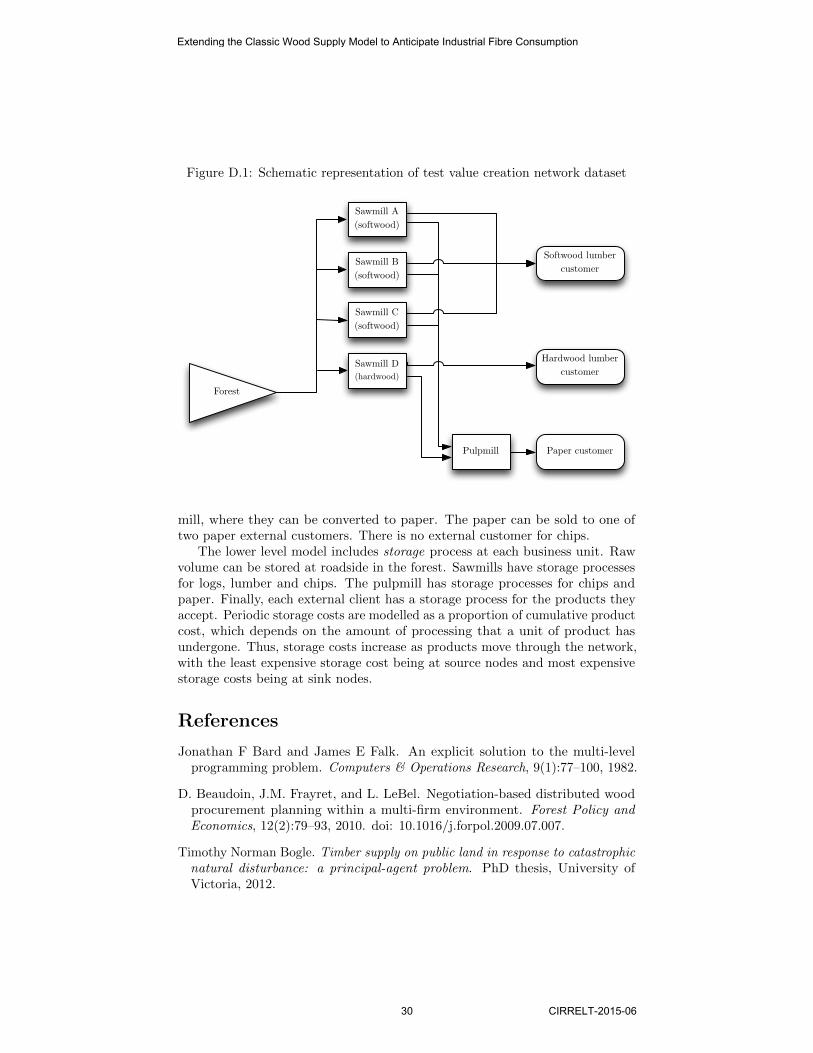
Figure D.1: Schematic representation of test value creation network dataset

Forest

Sawmill B(softwood)

Sawmill A(softwood)

Sawmill C(softwood)

Sawmill D(hardwood)

Pulpmill Paper customer

Softwood lumber customer

Hardwood lumber customer

mill, where they can be converted to paper. The paper can be sold to one oftwo paper external customers. There is no external customer for chips.

The lower level model includes storage process at each business unit. Rawvolume can be stored at roadside in the forest. Sawmills have storage processesfor logs, lumber and chips. The pulpmill has storage processes for chips andpaper. Finally, each external client has a storage process for the products theyaccept. Periodic storage costs are modelled as a proportion of cumulative productcost, which depends on the amount of processing that a unit of product hasundergone. Thus, storage costs increase as products move through the network,with the least expensive storage cost being at source nodes and most expensivestorage costs being at sink nodes.

References

Jonathan F Bard and James E Falk. An explicit solution to the multi-levelprogramming problem. Computers & Operations Research, 9(1):77–100, 1982.

D. Beaudoin, J.M. Frayret, and L. LeBel. Negotiation-based distributed woodprocurement planning within a multi-firm environment. Forest Policy andEconomics, 12(2):79–93, 2010. doi: 10.1016/j.forpol.2009.07.007.

Timothy Norman Bogle. Timber supply on public land in response to catastrophicnatural disturbance: a principal-agent problem. PhD thesis, University ofVictoria, 2012.


30 CIRRELT-2015-06

Tony Byrne, Cameron Stonestreet, Brian Peter, et al. Characteristics andutilization of post-mountain pine beetle wood in solid wood products. Themountain pine beetle: A synthesis of biology, management, and impacts onlodgepole pine. Natural Resources Canada, Canadian Forest Service, PacificForestry Centre, pages 233–253, 2006.

Canadian Council of Forest Ministers. Defining Sustainable Forest Managementin Canada: Criteria and Indicators. Technical Report Fo75-3/5-2003E, NaturalResources Canada, Canadian Forest Service, 2003.

Canadian Council of Forest Ministers. A Vision for Canada’s Forests: 2008 andbeyond. Technical Report Fo4-23/2008E-PDF, Natural Resources Canada,Canadian Forest Service, 2008.

Benoıt Colson, Patrice Marcotte, and Gilles Savard. An overview of bileveloptimization. Annals of operations research, 153(1):235–256, 2007. doi:10.1007/s10479-007-0176-2.

L.S. Davis, K.N. Johnson, P.S. Bettinger, and T.E. Howard. Forest Management:To Sustain Ecological, Economic, and Social Values, chapter 13, page 754.McGraw Hill, 2001.

Stephan Dempe. Annotated bibliography on bilevel programming and mathe-matical programs with equilibrium constraints. Optimization, 52(3):333–359,2003.

Jose Fortuny-Amat and Bruce McCarl. A representation and economic interpre-tation of a two-level programming problem. The Journal of the OperationalResearch Society, 32(9):783–792, 1981.

D. Fudenberg and J. Tirole. Game Theory. MIT Press, 1991. ISBN9780262061414.

E. Gunn. Some Perspectives on Strategic Forest Management Models and theForest Products Supply Chain. INFOR: Information Systems and OperationalResearch, 47(3):261–272, 2009. ISSN 0315-5986.

Eldon Gunn. Models for strategic forest management. In Andres Weintraub,Carlos Romero, Trond Bjørndal, and Rafael Epstein, editors, Handbook ofOperations Research in Natural Resources, chapter 16, pages 317–341. SpringerScience+Business Media, 2007.

Nigel Howard. Paradoxes of rationality: theory of metagames and politicalbehavior. MIT Press, 1971.

W. Jerbi, J. Gaudreault, S. D’Amours, M. Nourelfath, S. Lemieux, P. Marier, andM. Bouchard. Optimization/simulation-based framework for the evaluationof supply chain management policies in the forest product industry. In 2012IEEE International Conference on Systems, Man, and Cybernetics (IEEESMC 2012). IEEE (accepted), 2012.


CIRRELT-2015-06 31

Jean-Jaques Laffont and David Martimort. The theory of incentives: theprincipal-agent model. Princeton University Press, 2002. ISBN 9781400829453.

M. K. Luckert and T. Williamson. Should sustained yield be part of sustainableforest management? Canadian Journal of Forest Research, 35(2):356–364,2005.

Martin K. Luckert and David Haley. The allowable cut effect as a policyinstrument in Canadian forestry. Canadian Journal of Forest Research, 25(11):1821–1829, 1995.

A.H. Mathey, H. Nelson, and C. Gaston. The economics of timber supply: Doesit pay to reduce harvest levels? Forest Policy and Economics, 11(7):491–497,2009.

National Forestry Database, 2014. URL http://nfdp.ccfm.org. Last accessedon September 1, 2014.

Gregory Paradis, Luc LeBel, Sophie D’Amours, and Mathieu Bouchard. Onthe risk of systematic drift under incoherent hierarchical forest managementplanning. Canadian Journal of Forest Research, 43(5):480–492, 2013. doi:10.1139/cjfr-2012-0334.

Frederic Raulier, Narayan Dhital, Pierre Racine, Rebecca Tittler, and AndrewFall. Increasing resilience of timber supply: How a variable buffer stock oftimber can efficiently reduce exposure to shortfalls caused by wildfires. ForestPolicy and Economics, 2014.

C. Schneeweiß. Distributed Decision Making. Springer Verlag, 2003.

Tennessee Trent, Val Lawrence, Kathy Woo, et al. A wood and fibre quality-deterioration model for mountain pine beetle-killed trees by biogeoclimaticsubzone. 2006.

Dajun Yue and Fengqi You. Game-theoretic modeling and optimization ofmulti-echelon supply chain design and operation under stackelberg game andmarket equilibrium. Computers & Chemical Engineering, 71:347–361, 2014.

Wenyuan Zhai, Yingzi Zhao, Xiangru Lian, Mingming Yang, and Fadian Lu. Man-agement planning of fast-growing plantations based on a bi-level programmingmodel. Forest Policy and Economics, 38:173–177, 2014.


32 CIRRELT-2015-06

extending the classic wood supply model to …extending the classic wood supply model to anticipate...

Documents