Extended Kalman Filter for Large Scale VesselsTrajectory Tracking in Distributed Stream

Processing Systems

Katarzyna Juraszek1, Nidhi Saini2, Marcela Charfuelan2, Holmer Hemsen2,and Volker Markl1,2

1 Technische Universitat Berlin, Straße des 17. Juni 135, 1062, Berlin, Germanyhttps://www.tu-berlin.de

2 DFKI GmbH, Alt-Moabit 91c, 10559, Berlin, Germanyhttps://www.dfki.de

Abstract. The growing number of vehicle data being constantly re-ported by a variety of remote sensors, such as Automatic IdentificationSystems (AIS), requires new data analytics methods that can operateat high data rates and are highly scalable. Based on a real-life dataset from maritime transport, we propose a large scale vessels trajectorytracking application implemented in the distributed stream processingsystem Apache Flink. By implementing a state-space model (SSM) - theExtended Kalman Filter (EKF) - we firstly demonstrate that an imple-mentation of SSMs is feasible in modern distributed data flow systemsand secondly we show that we can reach a high performance by leverag-ing the inherent parallelization of the distributed system. In our experi-ments we show that the distributed tracking system is able to handle athroughput of several hundred vessels per ms. Moreover, we show thatthe latency to predict the position of a vessel is well below 500 ms onaverage, allowing for real-time applications.

Keywords: time-series · state-space models · Extended Kalman Filter· stream processing · spatio-temporal data · remote sensing systems.

1 Introduction

Analysing and understanding of maritime traffic is a topic of increasing interest,due to its direct implications on security and safety, as well as on environmentaland socio-economic factors. Nowadays, there is a growing number of ship report-ing technologies and remote sensing systems such as the Automatic IdentificationSystem (AIS), Long Range Identification and Tracking (LRIT), radar trackingor Earth Observation. Each of these technologies provides spatio-temporal ves-sel positioning data that contributes to better monitoring of maritime transport.The AIS technology has become a standard in the industry, being mandatoryfor ships in international voyages, such as cargo vessels, fishing vessels exceed-ing certain size as well as all passenger vessels, regardless of their size. TheAIS information provided by vessels, as a stream of tuples, includes kinematic

2 Juraszek K., Saini N., Charfuelan M., Hemsen H., Markl V.

information such as latitude, longitude, speed and course, voyage informationincluding destination port and estimated time of arrival, as well as static datasuch as size and type of a ship. The AIS technology, which was originally in-troduced for collision avoidance, is currently also used for vessel tracking, vesselbehaviour identification and anomaly detection [3].

State-space models (SSMs) are a popular methodology to model how differ-ent phenomena change over time [16]. The term state-space was originally coinedby Kalman (1960), and applied to the field of control engineering. An SSM is arepresentation of some physical system, where input, output and state variablesare related by first-order differential equations. The state variables depend oninput variables, while the output variables depend on the values of the statevariables. The SSM methodology has been successfully applied in various fields,including engineering, statistics, computer science and economics. The KalmanFilter is well-known for being one of the most powerful techniques for state esti-mation. The purpose of the algorithm is to provide an estimation with minimumerror variance. The nonlinear version of the algorithm, the so called ExtendedKalman Filter (EKF) is widely used to estimate position in GPS receivers [13] orfor robot tracking [17]. The academic community, using EKF in practice, usuallyfocuses on motion of robots in a constrained space. In contrast, applying statespace models to vessels’ tracking data imposes further challenges such as infre-quent or discontinued observations, arbitrary or noisy trajectories and erraticmovements.

Distributed computing helps in processing large amounts of raw data in real-time and in a timely manner by parallelising the computation, distributing thedata and handling failures [11]. In addition, distributed stream processing solu-tions are helping to overcome the main obstacles of real-time processing, whichare achieving the consistency of states across the system as well as fault recov-ery, requiring long recovery times. Thanks to these features, new distributedprocessing engines, which provide users with the scalable execution of data anal-ysis tasks are arising [12]. The main goal of current and popular engines suchas Hadoop [2], Apache Spark [7] or Apache Flink [6] is to enable developers towrite distributed data analysis applications in an easy and efficient manner.

In this paper we propose an implementation of the EKF in a distributedstream processing system for real-time trajectory tracking of many vessels inparallel. In our experiments each vessel provides a stream of remote sensing AISdata, which is used to create and continuously update its SSM. This way we areable to estimate in real-time a new position of each vessel. We show that in ouruse case the distributed tracking system is able to handle a throughput of 200vessels/ms and requires a latency below 500 ms on average to predict the nextposition of a vessel.

The paper is organised as follows. First we summarize the selection of re-lated work on processing streams, real-time data tracking and EKF. Section 3includes the theory behind the EKF as well as the practical implementation ofthe algorithm in Apache Flink. Section 4 describes the technical setup behind theEKF in the distributed environment. In the subsequent part, Section 5, the data

EKF for Large Scale Vessels Trajectory Tracking in DSPS 3

set characteristics, accuracy results of the experiments as well as performanceevaluation is given, followed by the conclusion in the last section.

2 Related Work

As reported in the survey paper [24], AIS data is used nowadays in several worksfor mining relevant aspects of navigation such as safety of seafaring, namely traf-fic anomaly detection, route estimation, collision prediction, and path planning.In this survey several techniques are reported, including EKF as a learning-model-based method for route estimation.

EKF has been used for tracking vessels in many works. For example in Pereraand Soares [21] an EKF algorithm is proposed as a vessel state estimator due toits capabilities of fusing nonlinear system kinematics with a given set of noisymeasurements. They use the EKF not only for state estimation (i.e. position,velocity and acceleration) but also for trajectory prediction. Their experimentsare performed in Matlab and only with simulated data.

SSMs and Kalman Filtering have been studied and implemented in vari-ous tools for a long time but mainly applied to single machines and relativelysmall sets of batch data. Several traditional tools get short on processing thebig amounts of data that can be generated nowadays or simply they are notcapable of processing stream data. Therefore some researchers have started toconsider the possibility to use and implement these techniques in large scaledistributed data flow systems. For example Sheng et al. [23] implemented anextended Kalman filter (a recursive filter) using the MapReduce framework, inorder to perform prediction in an industrial setting. Moussa [19] used ApacheSpark Streaming to implement a scalable application for real-time predictionof vessels’ future locations. The method used in this work for estimating a newposition is based on a scalable computation of trip patterns, which are efficientlyqueried using a geo-hashing index. This work also uses the DEBS Challenge 2018data, but unfortunately it does not report thorough experiments on throughputor latency.

Another interesting work that already addresses the problem of processingstreams of AIS data in real-time is reported by Brandt and Grawunder [9],where the whole trajectories of a vessel and its current neighbors are predictedin order to avoid critical situations, such as two vessels being too close to eachother. In the setup of this work, the real-time arrival and processing of the datapoints is simulated by sampling the data and then estimating the trajectory ofa vessel ten minutes into the future. In contrast to the approach presented inour paper, the authors calculate ten locations per predicted trajectory ratherthan the next location of the vessel. The authors admit that the simple linearextrapolation used in their work to predict the future trajectories of the movingobjects leads to non-optimal predictions, especially when a vessel is turning. Inaddition, the authors perform the computation on a single machine and thereforethe computationally demanding queries are far from delivering the results in nearreal-time. Dalsnes et al. [10] present a similar data-driven approach using cubic

4 Juraszek K., Saini N., Charfuelan M., Hemsen H., Markl V.

spline interpolation of trajectories sampled from an AIS historical database.They predict vessel’s position 5 to 15 minutes into the future also using therecent past trajectory of the vessel. This work relies heavily on the availabilityof historical data and there is no information regarding its use in a streamingfashion or real-time.

3 The Extended Kalman Filter

We apply distributed data flow processing to analyse kinematic information,such as latitude, longitude, speed and course from multiple vessels in parallel.While processing the data, we apply the Extended Kalman Filter to real-timestream data in order to estimate the next position of a vessel. To the best of ourknowledge, we present the first implementation of an Extended Kalman Filteron the distributed data flow system Apache Flink.

3.1 EKF in Theory

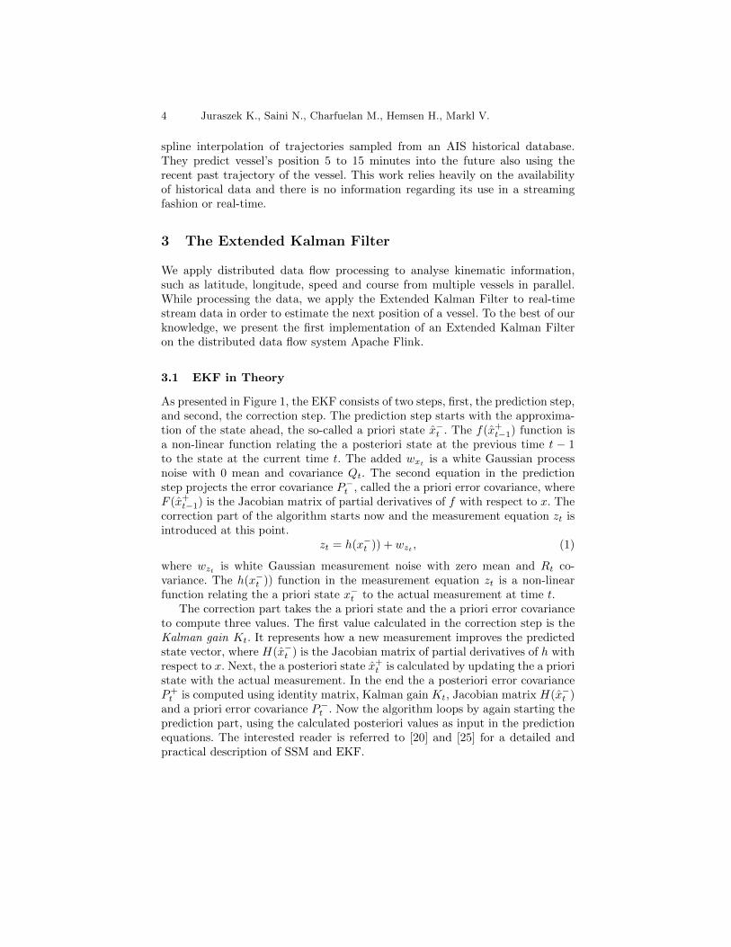
As presented in Figure 1, the EKF consists of two steps, first, the prediction step,and second, the correction step. The prediction step starts with the approxima-tion of the state ahead, the so-called a priori state x−t . The f(x+t−1) function isa non-linear function relating the a posteriori state at the previous time t − 1to the state at the current time t. The added wxt

is a white Gaussian processnoise with 0 mean and covariance Qt. The second equation in the predictionstep projects the error covariance P−

t , called the a priori error covariance, whereF (x+t−1) is the Jacobian matrix of partial derivatives of f with respect to x. Thecorrection part of the algorithm starts now and the measurement equation zt isintroduced at this point.

zt = h(x−t )) + wzt , (1)

where wzt is white Gaussian measurement noise with zero mean and Rt co-variance. The h(x−t )) function in the measurement equation zt is a non-linearfunction relating the a priori state x−t to the actual measurement at time t.

The correction part takes the a priori state and the a priori error covarianceto compute three values. The first value calculated in the correction step is theKalman gain Kt. It represents how a new measurement improves the predictedstate vector, where H(x−t ) is the Jacobian matrix of partial derivatives of h withrespect to x. Next, the a posteriori state x+t is calculated by updating the a prioristate with the actual measurement. In the end the a posteriori error covarianceP+t is computed using identity matrix, Kalman gain Kt, Jacobian matrix H(x−t )

and a priori error covariance P−t . Now the algorithm loops by again starting the

prediction part, using the calculated posteriori values as input in the predictionequations. The interested reader is referred to [20] and [25] for a detailed andpractical description of SSM and EKF.

EKF for Large Scale Vessels Trajectory Tracking in DSPS 5

Prediction step

1. Calculate a priori statex−t = f(x+

t−1) + wxt

2. Calculate a priori error covarianceP−t = F (x+

t−1)P+t−1F (x+

t−1)T + Qt

Correction step

1. Compute Kalman GainKt = P−

t H(x−t )T ×(H(x−

t )P−t H(x−

t )T +Rt)−1

2. Calculate a posteriori state by correcting x−t

x+t = x−

t + Kt(zt − h(x−t ))

3. Calculate a posteriori error covarianceby correcting P−

t

P+t = (I −KtH(x−

t )) · P−t

(Only as first step:)Initial estimates for x+

t−1 and P+t−1

Fig. 1: Graphical representation of the Extended Kalman Filter operations (adaptedfrom [25]).

3.2 EKF in Practice

One of the prerequisites for implementing EKF in practice is the a priori knowl-edge of the type of movement of an object. In case of tracking, such as vesselson waters, no a priori knowledge of the directions of the target is generally avail-able, therefore in our case the behaviour of vessels is approximated by a constantvelocity model. Since ocean vessels tend to follow a slow parabolic-type move-ment, where fast changing manoeuvres are not present, this assumption goes inline with other scholars’ findings [22]. In order to use the coordinate data, thegeodetic coordinates (WGS 84), which are not suitable for data processing areconverted so that the next location of a vessel is not predicted with respect tolongitude and latitude values, but rather as a latitude and longitude distance inmeters from the point where last position of a ship was reported.

EKF Parameters Initialization In order to start the EKF for the first time,two parameters need to be initialized, a posteriori state and a posteriori errorcovariance. Since the starting point of the route is known, the a posteriori errorcovariance is set to a small value (0.01) on the main diagonal of the a poste-riori error covariance matrix. The initial state estimate is set to zero, as thevalues will be replaced with the next run of the EKF. Two other parameters,being reused by the EKF on each run, are Q and R, which are the process noisecovariance matrix and measurement noise covariance matrix. When using theEKF algorithm for tracking of moving objects, Q represents possible accelera-tions that allow the tracked object to deviate from constant velocity. Following

6 Juraszek K., Saini N., Charfuelan M., Hemsen H., Markl V.

the assumptions of the acceleration process noise, which can be assumed to be8.8 m/s2 and assuming 2 rad/s as maximum turn rate for the vehicle, the follow-ing values are set on the main diagonal of the process noise covariance matrix:[(0.5 ·8.8 ·∆t2)2, (0.5 ·8.8 ·∆t2)2, (2 ·∆t)2), (8.8 ·∆t)2], where ∆t is the time differ-ence in seconds between the current and the previous measurement [8]. The lastparameter to be initialised is the measurement noise covariance matrix R. Themeasurement noise covariance R can be defined using the standard deviation ofa GPS measurement, which is assumed to be 6.0. The bigger the value, the less”trust” is given to the sensor readings [15].

EKF Implementation In the EKF algorithm implemented for the purpose offinding the next position of a vessel, the belief state to be estimated has fourvariables: cumulative longitude distance x, cumulative latitude distance y (bothcalculated from the departure point), heading, and velocity of a vessel at a giventime t. The algorithm starts with calculating the a priori state. To do so, the aposteriori state from previous measurements is used with the constant velocitymodel to predict the new a priori state. The a priori state has the following form:

x−t =

x−ty−tψ−t

υ−t

=

x+t−1 +∆t · υ+t−1 · cos(ψ+

t−1)y+t−1 +∆t · υ+t−1 · sin(ψ+

t−1)(ψ+

t−1) mod (2 · π) − πυ+t−1

(2)

where x−t is the predicted a priori state, x−t and y−t are respectively the cumula-tive longitude and latitude distance in meters from the departure port, ∆t is thetime difference in seconds between the current and the previous measurement,ψ+t−1 is the heading of a vessel and υ+t−1 is the velocity of a vessel in meters per

second.To calculate the a priori error covariance, the F (x+t−1), which is the Jacobian

matrix of partial derivatives of f(x+t−1) with respect to x, needs to be calculatedfirst.

F (x+t−1) =

1 0 −∆t · υ+t−1 · sin(ψ+

t−1) ∆t · cos(ψ+t−1)

0 1 ∆t · υ+t−1 · cos(ψ+t−1) ∆t · sin(ψ+

t−1)0 0 1 00 0 0 1

(3)

The a priori error covariance is then predicted following the formula given forP−t . The input in the calculation of the a posteriori state is the actual mea-

surement data zt and the a priori state x−t . In our EKF implementation, theactual measurement data is the actual longitude and latitude distance from thedeparture point, calculated as the cumulative sum of all the distances betweenthe measurements until this point in time.

zt =

[measured cumulative longitudinal distance

measured cumulative latitude distance

](4)

EKF for Large Scale Vessels Trajectory Tracking in DSPS 7

The remaining parts of the algorithm are calculated following the equations fromFigure 1.

4 Distributed Pipeline

4.1 Technical setup

The technical setup of the processing pipeline for this work is presented in Figure2. The real-time arrival of the time-series data is simulated using Apache Kafkaand the distributed computing of the next location prediction given by the EKFis leveraged with the use of Apache Flink.

Fig. 2: Detailed Kafka Flink pipeline.

4.2 EKF in the distributed environment

Since every non-trivial streaming application is stateful, applying the EKF in adistributed environment using Flink requires working with the state abstraction.States are an important feature but also have a serious performance impact onthe processing in distributed data flow systems, as they require synchronizationacross machines and need to be managed in a fault-tolerant way in case ofmachine failures. A stateful application remembers certain events or intermediateresults, which can be accessed later, for instance when a new event is arriving [6].Given the recursive nature of the EKF algorithm, where the a posteriori valuescalculated in the correction step are further used in the prediction step when anew event arrives, the use of Keyed State operators [4] is crucial for implementingthis algorithm in a distributed system. We use four different states in our work:

– The first state prevKalmanParams is used to store a tuple consisting of aposteriori state and a posteriori error covariance calculated in the Correctionstep.

– The second state prevTimestamp stores the timestamp of the last arrivingevent so that the time difference (∆t) needed for the prediction of the apriori state can be calculated upon arrival of the next event.

8 Juraszek K., Saini N., Charfuelan M., Hemsen H., Markl V.

– The third state prevGeoPoints remembers the last position reported in thelast event in order to calculated the distance travelled.

– The fourth state prevCumSum stores the cumulative sum of distance travelledfrom the reported departure port.

Each of these states is updated on every input tuple whenever an event arrives.The state values from the previous run are fed to the current calculation. In theimplementation of the EKF algorithm the Managed Key State ValueState<T>was used, which is a state scoped to the key of the current input element. It meansthat every keyed stream, belonging to one trajectory, will have a correspondingstate. This type of state can keep the value, which can be then retrieved andupdated per key. In our case one key corresponds to one vessel.

5 Data and Experiments

The data set used in the vessels trajectory tracking use case, was provided byMarineTraffic during the 2018 DEBS Grand Challenge [1] and includes the geo-location data, in terms of latitude and longitude, of vessels departing from 25ports in the Mediterranean Sea. The data is provided as a continuous streamof tuples. A ship sends a tuple according to its behaviour based on the AISspecifications. Each these tuples includes also the name of the port of origin,unique ID of the vessel, time stamp, vessel’s course, heading and draught. Thedata include several types of vessels, corresponding to 503 trajectories obtainedduring a period of approximately three months in 2015 (10-03-15 13:13 to 19-05-15 7:32). Many of the vessels report their position every two minutes, but somehave very irregular periods, including long periods of time (several hours) withno report.

The experiments are conducted on a single server machine with 48 CPUs, 2.0Ghz, 126 GB of RAM, running Ubuntu 16.04, Apache Kafka (v. 2.11) and ApacheFlink (v. 1.8). Following the recommendations in the Flink documentation, wefixed the number of Flink task slots to 48. Thus in our experiments the level ofparallelism is given by the number of slots or CPUs used [5].

In the following we evaluate our system according to accuracy and large scaleperformance. In the first experiment, Section 5.1, we calculate the next positionprediction error for every point of the 503 trajectories in the data. In the secondexperiment, Section 5.2, we evaluate the performance of the system in terms ofevent and processing time latency as well as ingestion rate.

5.1 Accuracy Evaluation

The result of the point prediction using the Extended Kalman Filter is a longi-tude and latitude pair of the next vessel’s position. For evaluating accuracy weuse the RMSE, which is also used for example in [10] to analyse the proximityof the mean of predicted values to the true value. We apply RMSE to calculatethe prediction error for latitude and longitude values but also for distance, that

EKF for Large Scale Vessels Trajectory Tracking in DSPS 9

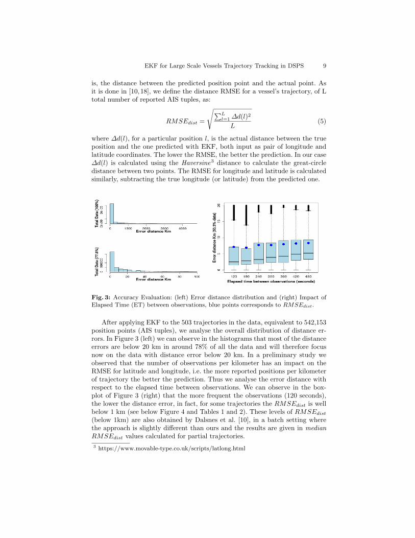
is, the distance between the predicted position point and the actual point. Asit is done in [10,18], we define the distance RMSE for a vessel’s trajectory, of Ltotal number of reported AIS tuples, as:

RMSEdist =

√∑Ll=1∆d(l)2

L(5)

where ∆d(l), for a particular position l, is the actual distance between the trueposition and the one predicted with EKF, both input as pair of longitude andlatitude coordinates. The lower the RMSE, the better the prediction. In our case∆d(l) is calculated using the Haversine3 distance to calculate the great-circledistance between two points. The RMSE for longitude and latitude is calculatedsimilarly, subtracting the true longitude (or latitude) from the predicted one.

Fig. 3: Accuracy Evaluation: (left) Error distance distribution and (right) Impact ofElapsed Time (ET) between observations, blue points corresponds to RMSEdist.

After applying EKF to the 503 trajectories in the data, equivalent to 542,153position points (AIS tuples), we analyse the overall distribution of distance er-rors. In Figure 3 (left) we can observe in the histograms that most of the distanceerrors are below 20 km in around 78% of all the data and will therefore focusnow on the data with distance error below 20 km. In a preliminary study weobserved that the number of observations per kilometer has an impact on theRMSE for latitude and longitude, i.e. the more reported positions per kilometerof trajectory the better the prediction. Thus we analyse the error distance withrespect to the elapsed time between observations. We can observe in the box-plot of Figure 3 (right) that the more frequent the observations (120 seconds),the lower the distance error, in fact, for some trajectories the RMSEdist is wellbelow 1 km (see below Figure 4 and Tables 1 and 2). These levels of RMSEdist

(below 1km) are also obtained by Dalsnes et al. [10], in a batch setting wherethe approach is slightly different than ours and the results are given in medianRMSEdist values calculated for partial trajectories.

3 https://www.movable-type.co.uk/scripts/latlong.html

10 Juraszek K., Saini N., Charfuelan M., Hemsen H., Markl V.

Fig. 4: Accuracy Evaluation: two trajectories corresponding to shipID-28 (leftRMSEdist=334.14m, mean ET=167.2 sec.) and shipID-57 (right RMSEdist=664.23m,mean ET=667.9 sec. ), blue points correspond to actual values and red points to theones predicted with EKF.

Fig. 5: Accuracy Evaluation: two trajectories corresponding to shipID-2 (left RMSEdist=4755.24m, mean ET=1279.7 sec.) and shipID-95 (rightRMSEdist=20279.30m, mean ET=1644.7 sec.), blue points correspond to actualvalues and red points to the ones predicted with EKF.

Table 1: Accuracy evaluation: Distance error quantiles for selected ship trajectories.

Ship IDDistance Error Quantiles

Min 1Q Median Mean 3Q Max

28 40.0 133.4 233.5 271.5 361.4 1978.157 0.3 17.4 45.2 363.0 612.7 6442.52 1.0 331.1 580.1 1110.0 889.1 105040.395 601.9 2251.2 4844.1 9034.3 11213.3 477542.5

EKF for Large Scale Vessels Trajectory Tracking in DSPS 11

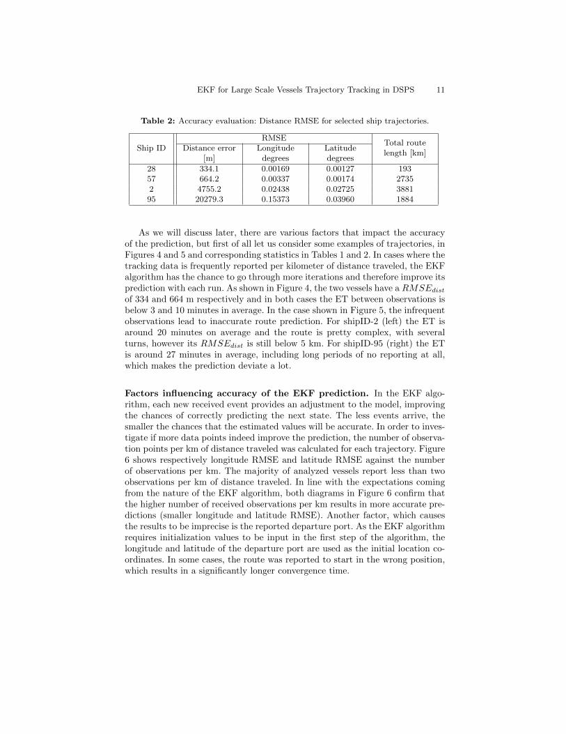
Table 2: Accuracy evaluation: Distance RMSE for selected ship trajectories.

Ship IDRMSE

Total routelength [km]

Distance error[m]

Longitudedegrees

Latitudedegrees

28 334.1 0.00169 0.00127 19357 664.2 0.00337 0.00174 27352 4755.2 0.02438 0.02725 388195 20279.3 0.15373 0.03960 1884

As we will discuss later, there are various factors that impact the accuracyof the prediction, but first of all let us consider some examples of trajectories, inFigures 4 and 5 and corresponding statistics in Tables 1 and 2. In cases where thetracking data is frequently reported per kilometer of distance traveled, the EKFalgorithm has the chance to go through more iterations and therefore improve itsprediction with each run. As shown in Figure 4, the two vessels have a RMSEdist

of 334 and 664 m respectively and in both cases the ET between observations isbelow 3 and 10 minutes in average. In the case shown in Figure 5, the infrequentobservations lead to inaccurate route prediction. For shipID-2 (left) the ET isaround 20 minutes on average and the route is pretty complex, with severalturns, however its RMSEdist is still below 5 km. For shipID-95 (right) the ETis around 27 minutes in average, including long periods of no reporting at all,which makes the prediction deviate a lot.

Factors influencing accuracy of the EKF prediction. In the EKF algo-rithm, each new received event provides an adjustment to the model, improvingthe chances of correctly predicting the next state. The less events arrive, thesmaller the chances that the estimated values will be accurate. In order to inves-tigate if more data points indeed improve the prediction, the number of observa-tion points per km of distance traveled was calculated for each trajectory. Figure6 shows respectively longitude RMSE and latitude RMSE against the numberof observations per km. The majority of analyzed vessels report less than twoobservations per km of distance traveled. In line with the expectations comingfrom the nature of the EKF algorithm, both diagrams in Figure 6 confirm thatthe higher number of received observations per km results in more accurate pre-dictions (smaller longitude and latitude RMSE). Another factor, which causesthe results to be imprecise is the reported departure port. As the EKF algorithmrequires initialization values to be input in the first step of the algorithm, thelongitude and latitude of the departure port are used as the initial location co-ordinates. In some cases, the route was reported to start in the wrong position,which results in a significantly longer convergence time.

12 Juraszek K., Saini N., Charfuelan M., Hemsen H., Markl V.

Fig. 6: Accuracy Evaluation: RMSE for Longitude and Latitude.

5.2 Performance Evaluation

In our large scale performance experiment we start simulating the streamingprocess by injecting the data into Kafka using several topics. Each Kafka topicis then read as a stream data source by Apache Flink. Each tuple in the streamsource is processed by Flink using its event time, i.e. the timestamp when theposition is reported. In the data, on average 10 vessels report their position atthe same time with peaks of up to 50 different vessels reporting their positionsimultaneously. This means that our processing system must be able to trackin real time many vessels at the same time. In order to cover this situation andstress the system even more, we replicated four times the input data assigningdifferent ships id. In this way we simulate the processing of more than 2000trajectories with peaks of maximum 200 vessels simultaneously reporting theirposition.

According to the benchmarking study of Karimov et al. [14], in modern dis-tributed stream processing systems two notions of time are distinguished: event-and processing-time latencies. From this study we use the following metrics:

– event-time latency, which measures the time that a given event has spent ina queue waiting to be processed. In our case it is the time a tuple spent inthe Kafka queue until the EKF operator is able to produce a new positionprediction for this tuple.

– processing-time latency, which measures the time it took for the event to beprocessed by the streaming system, what in our case means the time it takesfor the EKF operator to produce an output.

– ingestion rate, which is the throughput of a streaming system and in ourcase is measured as the number of tuples per millisecond processed by theEKF operator in Flink.

As pointed out by Karimov et al. [14], in practical scenarios, event-time latencyis very important as it defines the time in which the user interacts with a givensystem and should be minimized. It should be noted that processing-time la-tency makes part of the event-time latency. Thus our objective is to find theconfiguration that minimizes the processing-time in our system.

EKF for Large Scale Vessels Trajectory Tracking in DSPS 13

As shown in our Kafka-Flink pipeline (see Figure 2) we use 8 Kafka topicsand 8 corresponding Flink sources. The input source in each Kafka topic is thedata replicated four times, which contains trajectories of more than 2000 vessels.Overall the system receives and processes 17.4 million AIS events.

We use the default configuration settings for Kafka, so the number of parti-tions per topic is 1. We change the level of parallelism from 1 to 48 and repeateach experiment five times, averaging the results afterwards. To be precise, par-allelism 1 means using only one slot or CPU, which is the equivalent of executingthe experiment on a single machine. The results are presented in Figure 7. Weuse logarithmic scale on the y-axis to facilitate comparison.

Fig. 7: Performance Evaluation: Boxplot of event-time latency and processing-timelatency in server machine using 8 Kafka topics and 8 Flink sources.

For a single machine (in Figure 7 number of slots equal to 1), we obtain on av-erage the highest processing-time latency and event-time latency. For parallelism2 we can observe that the processing-time latency decreases but the event-timelatency is also in the order of seconds, which is still too high for real time process-ing. The processing-time latency decreases significantly when increasing the levelof parallelism, with optimal latency values for this setting, between parallelism 4(mean 27.7 ms) and 8 (mean 37.1 ms). Using higher parallelism (parallelisation8) also helps us to reduce the event-time latency to a mean minimum of 574.7ms. We can observe that for parallelism above 2 the event-time latency is belowa second, which can be explained by an increase of the ingestion rate. Thereforein the following, we further investigate the ingestion rate in our system.

As a comparison in Figure 8 we show a boxplot of the ingestion rate in Flinkin terms of tuples per millisecond. We can observe that without parallelismthe ingestion rate on average is minimum with approx. 170 tuples/ms, whenincreasing the parallelism the ingestion rate is on average stable in approx. 200tuples/ms, reaching maximum rates of approx. 500 tuples/ms.

14 Juraszek K., Saini N., Charfuelan M., Hemsen H., Markl V.

Fig. 8: Performance evaluation: Boxplot of the average Flink ingestion rate in tuplesper millisecond.

There are several aspects that are interrelated and contribute to the overallperformance of the system. For example, for parallelism 2 the average ingestionrate is higher but the processing latency with only two processors is still high.The optimal configuration in our system is obtained with 8 slots. Although theingestion rate is stable at approximate 200 tuples/ms, by adding more than 8slots we do not gain any performance. Such behaviour could be explain by thefact that the overall input data (17.4 million AIS events) is not large enough, sowe do not benefit from increasing parallelism, but instead we introduce distri-bution overhead.

6 Conclusion

In line with the expectations coming from recursive nature of the EKF, wherepredictions are corrected upon the arrival of a next data point, the frequency ofevents reception turned out to be an important factor influencing the accuracyof prediction produced. The results show that the complexity or stability of theroutes are not the most important factor contributing to the accurate predic-tion of the vessels’ routes. Irrespective of the trajectory complexity, the highfrequency of the incoming sensor measurements as well as correct initialisationof the parameters can provide a precise estimation of even more complex routes.

Regarding large scale performance, we showed that using a distributed streamprocessing system we can process on average 200 different vessels’ positions perms (200 tuples/ms), and our system, under this rate, requires below 500 ms topredict the next position of a vessel. In our setting, this optimal performancewas obtained when using 8 Kafka topics and the corresponding 8 Flink sources.

EKF for Large Scale Vessels Trajectory Tracking in DSPS 15

Beyond this optimal value, when we increase the number of Kafka topics andFlink sources, the system introduces some overhead that is reflected on thelatencies.

As future work we will consider a more realistic scenario, where massivereal data is used and a setting in a cluster of computers. In a cluster settingwe should take into account the additional overhead due to the communicationbetween nodes, thus we will study the optimal combination of parallelism, Kafkatopics and ingestion rate, in particular when actual big sets in the order of GBsare used. Furthermore, we will address the issue of visualization in real timeincluding a dashboard for indicating various conditions of the vessels, such aselapsed time since last report, distance traveled or big error predictions whichmay correspond to possible anomalies.

Acknowledgements

This work was partly supported by the German Ministry for Education andResearch (BMBF) as Berlin Big Data Center (BBDC2) (grant no. 01IS18025A),the German Federal Ministry of Transport and Digital Infrastructure (BMVI)through the Daystream project (grant no. 19F2031A).

References

1. DEBS 2018 Grand Challenge. http://www.cs.otago.ac.nz/debs2018/calls/gc.html,accessed: 2018-11-27

2. Hadoop. http://hadoop.apache.org/, accessed: 2018-11-273. Alessandrini, A., Alvarez, M., Greidanus, H., Gammieri, V., Arguedas, V.F., Maz-

zarella, F., Santamaria, C., Stasolla, M., Tarchi, D., Vespe, M.: Mining vesseltracking data for maritime domain applications. In: 2016 IEEE 16th InternationalConference on Data Mining Workshops (ICDMW). pp. 361–367. IEEE (2016)

4. Apache Flink: Application Development, Working with State: https://ci.apache.org/projects/flink/flink-docs-stable/dev/stream/state/state.html, accessed: 2019-06-10

5. Apache Flink: Configuration: https://ci.apache.org/projects/flink/flink-docs-release-1.8/ops/config.html#configuring-taskmanager-processing-slots,accessed: 2019-06-10

6. Apache Flink: Fast and reliable large-scale data processing engine: http://flink.apache.org, accessed: 2018-11-27

7. Apache Spark: https://spark.apache.org/, accessed: 2018-11-278. Balzer, P.: Multidimensional Kalman-Filter. https://github.com/balzer82/

Kalman/ (2017), accessed: 2018-11-279. Brandt, T., Grawunder, M.: Moving object stream processing with short-time pre-

diction. In: Proceedings of the 8th ACM SIGSPATIAL Workshop on GeoStream-ing. pp. 49–56. ACM (2017)

10. Dalsnes, B.R., Hexeberg, S., Flaten, A.L., Eriksen, B.H., Brekke, E.F.:The Neighbor Course Distribution Method with Gaussian Mixture Mod-els for AIS-Based Vessel Trajectory Prediction. In: 2018 21st Interna-tional Conference on Information Fusion (FUSION). pp. 580–587 (Jul 2018).https://doi.org/10.23919/ICIF.2018.8455607

16 Juraszek K., Saini N., Charfuelan M., Hemsen H., Markl V.

11. Dean, J., Ghemawat, S.: Mapreduce: simplified data processing on large clusters.Communications of the ACM 51(1), 107–113 (2008)

12. He, B., Yang, M., Guo, Z., Chen, R., Su, B., Lin, W., Zhou, L.: Comet: batchedstream processing for data intensive distributed computing. In: Proceedings of the1st ACM symposium on Cloud computing. pp. 63–74. ACM (2010)

13. Jwo, D.J., Wang, S.H.: Adaptive fuzzy strong tracking extended kalman filteringfor gps navigation. IEEE Sensors Journal 7(5), 778–789 (2007)

14. Karimov, J., Rabl, T., Katsifodimos, A., Samarev, R., Heiskanen, H., Markl, V.:Benchmarking distributed stream data processing systems. In: 2018 IEEE 34th In-ternational Conference on Data Engineering (ICDE). pp. 1507–1518. IEEE (2018)

15. Kelly, A.: A 3d state space formulation of a navigation kalman filter for autonomousvehicles. Tech. rep., Carnegie-Mellon University Pittsburgh PA Robotics Institute(1994)

16. Korn, U.: A simple method for modelling changes over time. Casualty ActuarialSociety E-Forum (2018)

17. Lee, J.W., Kim, M.S., Kweon, I.S.: A kalman filter based visual tracking algo-rithm for an object moving in 3d. In: Proceedings 1995 IEEE/RSJ InternationalConference on Intelligent Robots and Systems. Human Robot Interaction and Co-operative Robots. vol. 1, pp. 342–347. IEEE (1995)

18. Lipka, M., Sippel, E., Vossiek, M.: An Extended Kalman Filter for Direct, Real-Time, Phase-Based High Precision Indoor Localization. IEEE Access 7, 25288–25297 (2019). https://doi.org/10.1109/ACCESS.2019.2900799

19. Moussa, R.: Scalable maritime traffic map inference and real-time prediction ofvessels’ future locations on apache spark. In: Proceedings of the 12th ACM Inter-national Conference on Distributed and Event-based Systems. pp. 213–216. ACM(2018)

20. Murphy, K.P.: Machine Learning: A probabilistic perspective. The MIT Press(2012)

21. Perera, L.P., Oliveira, P., Soares, C.G.: Maritime traffic monitoring based on vesseldetection, tracking, state estimation, and trajectory prediction. IEEE Transactionson Intelligent Transportation Systems 13(3), 1188–1200 (2012)

22. Perera, S., Suhothayan, S.: Solution Patterns for Realtime Streaming An-alytics. In: Proceedings of the 9th ACM International Conference on Dis-tributed Event-Based Systems. pp. 247–255. DEBS ’15, ACM, New York,NY, USA (2015). https://doi.org/10.1145/2675743.2774214, http://doi.acm.org/10.1145/2675743.2774214

23. Sheng, C., Zhao, J., Leung, H., Wang, W.: Extended kalman filter based echo statenetwork for time series prediction using mapreduce framework. In: 2013 IEEE 9thInternational Conference on Mobile Ad-hoc and Sensor Networks. pp. 175–180.IEEE (2013)

24. Tu, E., Zhang, G., Rachmawati, L., Rajabally, E., Huang, G.B.: Exploiting ais datafor intelligent maritime navigation: a comprehensive survey from data to method-ology. IEEE Transactions on Intelligent Transportation Systems 19(5), 1559–1582(2017)

25. Welch, P., Bishop, G.: An Introduction to the Kalman Filter (courseP-ack). http://www.cs.unc.edu/∼tracker/media/pdf/SIGGRAPH2001 CoursePack08.pdf (2001), accessed: 2018-11-27