Exponential sums, hypersurfaces with many

symmetries and Galois representations

Gabriel Chenevert

Department of Mathematics and Statistics

McGill University, Montreal

September 2008

A thesis submitted to McGill University in partial fulfilment

of the requirements of the degree of Doctor of Philosophy

c© Gabriel Chenevert, 2008

Contents

Table of contents . . . . . . . . . . . . . . . . . . . . . . . . . . . . . . . . . i

Abstract . . . . . . . . . . . . . . . . . . . . . . . . . . . . . . . . . . . . . . iii

Resume . . . . . . . . . . . . . . . . . . . . . . . . . . . . . . . . . . . . . . v

Acknowledgments . . . . . . . . . . . . . . . . . . . . . . . . . . . . . . . . . vii

Introduction 1

Notation 7

1 Linear representations 9

1.1 Generalities on representations . . . . . . . . . . . . . . . . . . . . . . . 10

1.2 Isotypic decomposition and multiplicities . . . . . . . . . . . . . . . . . 14

1.3 Representations of the symmetric group . . . . . . . . . . . . . . . . . 18

1.4 Galois representations . . . . . . . . . . . . . . . . . . . . . . . . . . . 21

1.5 Compatible systems . . . . . . . . . . . . . . . . . . . . . . . . . . . . . 27

2 Etale cohomology 31

2.1 Basic properties . . . . . . . . . . . . . . . . . . . . . . . . . . . . . . . 32

2.2 The trace formula and purity . . . . . . . . . . . . . . . . . . . . . . . 35

2.3 Smooth hypersurfaces . . . . . . . . . . . . . . . . . . . . . . . . . . . . 38

2.4 Smooth quadrics . . . . . . . . . . . . . . . . . . . . . . . . . . . . . . 42

2.5 Hypersurfaces with ordinary double points . . . . . . . . . . . . . . . . 46

3 Hypersurfaces with symmetries 51

3.1 Isotypic decomposition . . . . . . . . . . . . . . . . . . . . . . . . . . . 52

3.2 Symmetric hypersurfaces . . . . . . . . . . . . . . . . . . . . . . . . . . 56

3.3 Existence of special symmetric hypersurfaces . . . . . . . . . . . . . . . 68

3.4 The hypersurfaces Wm,n` . . . . . . . . . . . . . . . . . . . . . . . . . . 74

3.5 Some explicit computations . . . . . . . . . . . . . . . . . . . . . . . . 79

i

4 Distribution of exponential sums 81

4.1 Exponential sums as Fourier transforms . . . . . . . . . . . . . . . . . . 83

4.2 Equidistribution . . . . . . . . . . . . . . . . . . . . . . . . . . . . . . . 84

4.3 Exponential sums . . . . . . . . . . . . . . . . . . . . . . . . . . . . . . 86

4.4 Equidistribution results . . . . . . . . . . . . . . . . . . . . . . . . . . . 90

5 Comparing Galois representations 101

5.1 Isogeny and modularity . . . . . . . . . . . . . . . . . . . . . . . . . . . 102

5.2 Deviation groups . . . . . . . . . . . . . . . . . . . . . . . . . . . . . . 106

5.3 The method of quartic fields . . . . . . . . . . . . . . . . . . . . . . . . 110

5.4 The Faltings-Serre-Livne criterion . . . . . . . . . . . . . . . . . . . . . 115

5.5 Generalization . . . . . . . . . . . . . . . . . . . . . . . . . . . . . . . . 121

5.6 Listing quadratic extensions . . . . . . . . . . . . . . . . . . . . . . . . 130

5.7 Modularity of W 72 . . . . . . . . . . . . . . . . . . . . . . . . . . . . . . 134

Conclusion 145

Appendix 149

Bibliography 162

ii

Abstract

The main theme of this thesis is the study of compatible systems of `-adic Galois repre-

sentations provided by the etale cohomology of arithmetic varieties with a large group

of symmetries. A canonical decomposition of these systems into isotypic components

is proven (Section 3.1). The isotypic components are realized as the cohomology of

the quotient with values in a certain sheaf, thus providing a geometrical interpretation

for the rationality of the corresponding L-functions.

A particular family of singular hypersurfaces Wm,n` of degree ` and dimension

m + n − 3, admitting an action by a product of symmetric groups Sm × Sn, arises

naturally when considering the average moments of certain exponential sums (Chap-

ter 4); asymptotics for these moments are obtained by relating them to the trace of the

Frobenius morphism on the cohomology of the desingularization of the corresponding

varieties, following the approach of [38].

Two other closely related classes of smooth hypersurfaces admitting an Sn-action

are introduced in Chapter 3, and the character of the representation of the sym-

metric group on their primitive cohomology is computed. In particular, a certain

smooth cubic hypersurface of dimension 4 is shown to carry a compatible system of

2-dimensional Galois representations. A variant of the Faltings-Serre method is devel-

oped in Chapter 5 in order to explicitly determine the corresponding modular form,

whose existence is predicted by Serre’s conjecture. We provide a systematic treat-

ment of the Faltings-Serre method in a form amenable to generalization to Galois

representations of other fields and to other groups besides GL2.

iii

iv

Resume

Le theme principal de cette these est l’etude des systemes compatibles de represen-

tations galoisiennes `-adiques provenant de la cohomologie etale de varietes arith-

metiques admettant beaucoup de symetries. Une decomposition canonique de ces

systemes en composantes isotypiques est obtenue (section 3.1). Les composantes iso-

typiques sont decrites comme la cohomologie du quotient a valeurs dans un certain

faisceau, fournissant ainsi une interpretation geometrique de la rationalite des fonc-

tions L correspondantes.

Une famille specifique d’hypersurfaces Wm,n` de degre ` et dimension m+n−3, ad-

mettant une action du produit de groupes symetriques Sm×Sn, apparaıt naturellement

en lien avec les moments moyens de certaines sommes exponentielles (chapitre 4); le

comportement limite de ces moments est obtenu en considerant la trace du morphisme

de Frobenius sur la cohomologie de la desingularisation des varietes correspondantes,

suivant l’approche developpee dans [38].

Deux autres classes apparentees d’hypersurfaces lisses admettant une action du

groupe symetrique sont introduites au chapitre 3, et le caractere de la representation

de Sn sur leur cohomologie primitive est calcule. En particulier, dans le cas d’une cer-

taine hypersurface cubique de dimension 4, un systeme compatible de representations

galoisiennes de dimension 2 est obtenu. Une variante de la methode de Faltings-Serre

est developpee dans le chapitre 5 afin de determiner explicitement la forme modulaire

correspondante, dont l’existence est predite par la conjecture de Serre. Nous pro-

posons un traitement systematique de la methode de Faltings-Serre d’un point de vue

qui se prete a la generalisation a d’autres corps ainsi que d’autres groupes que GL2.

v

vi

Acknowledgments

First and foremost, I want to thank my supervisor Eyal Goren for his constant ded-

ication and support throughout the last few years. It was he who introduced me to

the beauty of zeta functions when I took his algebraic geometry class as a Masters

student, and through his guidance I have learned a lot both as a mathematical and

human being. For some reason he always seemed to believe in my potential, and with-

out his tacit encouragements and efforts to make me concretize it this thesis would

almost certainly never have seen the light of the day.

Thanks as well to all the other professors from whom I learned, both inside and

outside the classroom. Henri Darmon, Adrian Iovita, Hershy Kisilevsky, Francois

Bergeron and Pierre Colmez come to mind. Special thanks to Jean-Pierre Serre who

had the kindness of taking the time on two occasions to discuss some of his old work

with me, and for being an overall awesome and inspiring person on so many levels.

Let’s not forget everybody else, fellow students and post-docs, as well as support

staff, which helped make my years in McGill be a pleasant and fruitful experience.

A special mention goes to Carmen Baldonado, who with constant kindness always

managed to keep me afloat among the many pitfalls of the McGill administration,

despite me often not doing much to facilitate her task. Thanks also to Jan Nekovar

and the people at Chevaleret for welcoming me there for a few months in 2006.

I also have the chance of knowing a certain number of people with whom I spent

a lot of time talking about mathematical things, not necessarily directly related to

this thesis, and who double as dear friends: Remi Leclercq and Eveline Legendre, my

surrogate family for a year; Baptiste Chantraine, the one and only; Etienne Ayotte-

Sauve, the hipster bureaucrat; Alexandre Girouard, the small red guy; and Clement

Hyvrier, the articulate clumsy absurdist.

Thanks to those who read parts of this thesis and provided me with some helpful

comments about my mathematical statements or prose, notably Filippo Nuccio who

caught all sorts of small things in the first chapter.

vii

Thanks to the Fab Four, both those from Liverpool and those from Verdun, for

making my world a wonderful place to live in. And the late Elliott Smith, for bringing

me solace in times when it was most direly needed.

Thanks to those who sustained me financially during these years and made it

possible for me not to worry much about the many vicissitudes of material life, namely

NSERC, FQRNT, ISM, the McGill math department, and of course my parents.

Thanks to anybody else who might happen to be presently reading these acknowl-

edgements.

And to Kristel ma belle, without whom all of this would be utterly meaningless.

viii

Introduction

It is a natural and pervasive approach in science in general, and mathematics in

particular, to try to comprehend a complex object via its representations (in the

broad sense) in a simpler setting sharing some of the same features. For example,

one can try to understand a 3-dimensional geometrical object by projecting it onto

various 2-dimensional planes and assemble these projections to form a coherent image

of the initial object. In mathematics, much information about a complicated algebraic

structure can be gained by studying its homomorphisms into more concrete or well-

understood structures. Here, the complicated structure we have in mind is the Galois

group

GalQ = Gal(Q/Q)

of all field automorphisms of the algebraic closure Q of Q, and understanding its

structure is arguably the ultimate goal of algebraic number theory.

In general, given a group G, we can consider its actions on objects X belonging

to a certain category C, i.e. homomorphisms

G −→ AutC X.

For example, when the objects X are finite sets, we are led to consider homomor-

phisms from G to symmetric groups, i.e. (homomorphic) realizations of G as groups

of permutations. In this thesis we will mainly be considering linear representations

over a field E, which can be considered concretely as homomorphisms from G to a

group of matrices GLn(E).

In the case of GalQ, this approach has been very fruitful to date. Witness class

field theory (a standard reference is [45]), which essentially gives a description of all

the 1-dimensional representations of GalQ. The case of 2-dimensional representations

have been a subject of active research during the last decades, and have seen a number

of spectacular achievements. The most famous is certainly the proof by Wiles et al.

1

[66, 64, 6] of the Shimura-Taniyama conjecture, which states that the 2-dimensional

representations coming from elliptic curves defined over Q arise from modular forms.

More recently a full proof of Serre’s conjecture [54] was announced (completing [31]

which proves it for odd conductors), so that the same can be considered to be true

for all odd, absolutely irreducible representations over finite fields. These are only

the first steps in the far-reaching web of conjectures that encompasses the Langlands

program, according to which all Galois representations arising from geometry should

be automorphic.

If X is an algebraic variety defined over a number field K, the set X(K) of points

of X with coordinates in K carries a natural action of the absolute Galois group

GalK of K. This action, however, does not propagates to an action on any of the

invariants provided by algebraic topology since it is not continuous with respect to

the topology inherited by an embedding K → C – never mind the fact that X(K),

with the topology induced from X(C), is totally disconnected – let alone algebraic

morphisms. This was one of the impetuses for Grothendieck and his coworkers to

develop in the 1960’s the theory of schemes to supply an appropriate category, and

then to develop the machinery of etale cohomology, associating to X a compatible

system of `-adic representations

H•(X,Q`)

for the absolute Galois group GalK . Keeping in mind that representations into struc-

tures which share a certain likeness with the original one are bound to yield interesting

information, it is no surprise that these `-adic representations carry non-trivial arith-

metic information.

Let X be a smooth and proper variety defined over a finite field Fq with q ele-

ments. Weil [65] had the initial insight that the conjectures he formulated about the

behavior of the number of points |X(Fqr)| as r varies would follow formally from the

existence of a “good” cohomology theory in this context, what is nowadays called a

Weil cohomology theory. Among the various requirements that such a theory would

have to satisfy in order to parallel the properties of Betti cohomology, one of the fore-

most is the analogue of the Lefschetz fixed point formula for the Frobenius morphism

Frobq of X. Weil’s insight was that the set X(Fqr) of Fqr -rational points of X can

be interpreted as the fixed locus of the rth iterate of Frobq on X(Fq), and thus could

be studied via such a suitable cohomology theory. As a consequence, if X is an arith-

metic variety defined over a number field K, understanding its etale cohomology (as

a compatible system of `-adic representations of GalK) is essentially the same thing

2

as understanding how many points it has over all finite fields for which this question

makes sense.

The starting point for this thesis was the pair of papers [38, 39] published by Livne

in the 1980’s. In the first one, he settles a conjecture of Birch [4] about the average

distribution of exponential sums of the form

∑x∈Fq

exp

(2πi

p(ax3 + bx)

), a, b ∈ Fp, a 6= 0,

as p → ∞. Here “average limit distribution” means that for each p, we consider all

the values of the parameters a and b at the same time, then look at how this set

behaves as p grows. The average distribution of these exponential sums was studied

in [38] via its moments, and the key fact is that these moments can be expressed in

terms of the number of points on the projective varieties Wn ⊆ Pn−1 defined by the

pair of homogeneous equations

n∑i=1

xi =n∑i=1

x3i = 0.

These varieties are smooth when n is odd, but acquire singularities when n is even.

These singularities turn out to be ordinary double points, so the results of Schoen [49]

can be applied to describe the cohomology of the desingularization of Wn of Wn, thus

yielding asymptotics for the average moments of the exponential sums. In Chapter 4

we lay out a framework which allows to treat more general exponential sums, obtained

by specifying a certain set of weights for the monomials that appear, and relate

their average moments to the number of points on certain more general varieties

depending on these weights. One major difference is that the cubic exponential sums

above are real-valued, hence their distribution can be understood by considering a

single sequence of moments; the exponential sum we consider are complex-valued in

general, so that a 2-parameter family of moments is needed. For example, to study

the distribution of the exponential sums

∑x∈Fp

exp

(2πi

p(ax`+1 + bx)

), a, b ∈ Fp, a 6= 0,

where ` is a fixed prime, we are led to study the projective varieties Wm,n` ⊆ Pm+n−1

3

defined by the homogeneous equations

m∑i=1

xi −n∑j=1

yj =m∑i=1

x`+1i −

n∑j=1

y`+1j = 0.

In the second paper [39], Livne singled out the variety W10 (or W 0,102 in our nota-

tion) he considered in relation with the 10th moment of cubic exponential sums and

remarked that the middle-degree cohomology of its desingularization W10 has dimen-

sion 2, hence carries a compatible system of `-adic representations of GalQ. He then

took an educated guess at what should be the corresponding modular form, and pro-

ceeded to show it was indeed the case. This is really a statement about equivalence of

two `-adic Galois representations, one associated to the modular form and the other

on the cohomology of W10, and he proved that the two representations were equivalent

by using a criterion suggested by Serre, building on a previous remark of Faltings,

which allows to decide whether two continuous 2-adic Galois representations with even

trace and dimension 2 are equivalent or not by computing a finite number of traces.

At the time when work on this thesis started, the Serre conjecture was not expected

to yield anytime soon (at least by the author of this thesis), hence it seemed desirable

to come up with other such sporadic examples of modularity. The first task was to

find other 2-dimensional compatible systems of Galois representations “in nature”

(i.e., in the etale cohomology of some arithmetic variety) for which modularity was

not known. Since varieties having a cohomology group of dimension exactly 2 are

relatively few (for example, the only smooth irreducible hypersurfaces having this

property are curves of genus 1), it was natural to look for varieties with possibly

large cohomology, but which could be broken up in smaller pieces. It is a general

phenomenon that this is the case for objects having extra symmetries (e.g. elliptic

curves with complex multiplication, for which modularity was known [16] much before

the 1990’s).

However, even if (or rather, when) the full Serre conjecture is proven, such ex-

plicit examples of modularity for 2-dimensional “motives” over Q are still of interest.

For one, to be able to compute the level of the modular form corresponding to a

2-dimensional compatible system of representations arising from the cohomology of

a variety, one would need very precise information about the ramification of the rep-

resentation, and this information is often not readily available. As a consequence,

one would often have to settle for a crude upper bound on the level of the modular

form. In addition, being able to perform explicit proofs of modularity for dimension 2

4

representations of GalQ is certainly a good starting point in our ambition to do just

the same over other number fields, or for representations into other groups, such as

GL3, Sp4, . . . , for which no general modularity result is currently known.

This thesis deals with several topics that are interwoven by connections such as

mentioned above. We consider certain exponential sums and their moments; co-

homology of certain varieties with large automorphism group and their motivic de-

composition; generalization of the Faltings-Serre criterion and tests for modularity.

Throughout we put emphasis on explicit methods.

The first chapter starts with a discussion of linear group representations, both

of finite groups in characteristic 0, and of Galois groups over `-adic fields. Its goal

is mainly to set up the notation and lay down the basic concepts which will appear

throughout. The distinction between isomorphism and semisimple equivalence is dis-

cussed (Section 1.1) as most Galois representations coming from geometry are not

yet known to be semisimple. The isotypic decomposition of representations of finite

groups in characteristic 0 is then stated in a functorial way (Section 1.2) as we will

need it to prove the analogous statement in the category of compatible systems of `-

adic representations in Chapter 3. The representation theory of the symmetric group

is then briefly described (Section 1.3), before describing some of the features of Galois

representations (Section 1.4) such as ramification, Artin L-functions and Hodge-Tate

weights. In the last section we describe compatible systems of `-adic representations

(Section 1.5).

Chapter 2 is devoted to etale cohomology, with some of its formal properties

described in Section 2.1. The Grothendieck trace formula, which implies that the etale

cohomology groups of with values in Q` (or more generally in a compatible family

of λ-adic constructible sheaves) form a compatible system, is discussed together with

purity in Section 2.2. We then describe more concretely the cohomology of smooth

hypersurfaces (Section 2.3) and in particular of smooth quadric (Section 2.4), as well

as that of hypersurfaces with ordinary double points (Section 2.5), following [49].

The last three chapters contain the original contributions of this thesis. In Chap-

ter 3 we consider the linear representations on cohomology of a finite group which

acts on a variety. The main theoretical result, probably known to the experts, is

the isotypic decomposition of Theorem 3.1.4 for the compatible systems of Galois

representations arising in such a context, i.e. that the Galois representations on the

isotypic components are themselves compatible systems. This will be needed in order

to perform some of the explicit computations in Chapter 5. In Section 3.2 we define

5

two classes of hypersurfaces admitting an action by the symmetric group Sn by permu-

tation of the homogeneous coordinates. For a certain subclass of these hypersurfaces,

which we call special, we obtain a general formula for the character of the representa-

tion of Sn on primitive cohomology (Theorem 3.2.14). We discuss in Section 3.3 the

existence of such special hypersurfaces by providing some examples and describing

obstructions to their existence coming from the representation theory of Sn. We then

introduce in Section 3.4 the hypersurfaces Wm,n` alluded to above, related to the av-

erage moments of exponential sums appearing in Chapter 4. When smooth, Wm,n` is

a special hypersurface in the sense of Section 3.2; when singular, its only singularities

are ordinary double points (Proposition 3.4.4). In the last section we compute decom-

positions into irreducibles of the primitive cohomology of special hypersurfaces of low

dimension; in particular, the variety W 0,72 is seen to carry a 2-dimensional compatible

system, for which the corresponding modular form in computed in Chapter 5.

Chapter 4 carries out the discussion of moments of exponential sums mentioned

above. After a short motivating introduction (Section 4.1) and review of the needed

notions from measure theory (Section 4.2), the family of exponential sums under

consideration is defined in Section 4.3 and their moments are related to the number

of points on varieties closely related to the Wm,n` (Theorem 4.3.2). In Section 4.4

we put the machinery to work, the main result being an expression for the limits

of the average moments for exponential sums of weights 1, ` + 1, with ` a prime,

generalizing the results and method of proof from [38] in the case ` = 2.

Finally, the last chapter is devoted to the topic of algorithmically deciding whether

two `-adic Galois representations are semisimply equivalent or not. In the first sec-

tion we explain why even for 2-dimensional systems over Q such methods can still be

useful even if we admit the Serre conjecture. The basic object in the Faltings-Serre

method, the deviation group of two `-adic representations, is introduced in Section

5.2, following [57], and its basic properties are discussed. In the next section we

discuss a more concrete homomorphic image of the deviation group, which can some-

times be substituted for the deviation group, in particular for the application to the

modularity of W 0,72 we had in mind (see the remark there). In any case, we proceed

to discuss in Section 5.4 the Faltings-Serre-Livne criterion, which is used as a model

for our generalization in the next section (Theorem 5.5.13, using the group-theoretic

classification result of Theorem 5.5.11). We then write down some general facts about

quadratic extensions in Section 5.6 before proceeding with the explicit determination

of the modular form corresponding to W 0,72 (Theorem 5.7.7).

6

Notation

The use of certain symbols is hopefully mostly consistent in this thesis.

The semi-ring of natural integers (including 0) is denoted N, the ring of relative

integers Z, and the fields of rational, real and complex numbers Q, R and C, respec-

tively. Rational prime numbers are usually denoted by p or `. The field of `-adic

numbers is Q`, while the ring of `-adic integers is Z`. An abstract finite field with

q = pr elements is written Fq.

Number fields are usually denoted K or L or variations on these. If L/K is a Galois

extension of number fields, its Galois group is denoted Gal(L/K). The absolute Galois

group of K with respect to an implicitly fixed algebraic closure K will be referred to

as GalK . A Gothic p is usually used to denote a finite place in a number field K, i.e.

a nonzero prime ideal in its ring of integers OK , and its norm N(p) is the cardinality

of the residual field kp = OK/p. The notation Frobp always refers to the geometric

Frobenius at p; the arithmetic Frobenius substitution, should it be needed, will be

referred to as Frob−1p . The cyclotomic character is denoted χcycl.

The letter E is mostly reserved for fields of characteristic 0 which serve as co-

efficients for representations and such. The trace of a linear operator σ on a finite

dimensional vector space V over E will be denoted trσ or tr(σ | V ) if needed. Simi-

larly, its determinant is written detσ or det(σ | V ). A graded vector space V • =⊕

i Vi

is denoted with the use of a bullet, the grading being often implicit. If σ is an graded

endomorphism of V , it is understood that the trace and determinant of σ are to be

taken in the graded sense, i.e.

tr(σ | V •) =∑i

(−1)i tr(σ | V i), det(σ | V ) =∏i

det(σ | V i)(−1)i .

If E is a local number field, i.e. a finite extension of Q`, with maximal ideal λ,

the notation Eλ will be used for psychological clarity, and its ring of integers will be

called Oλ.

7

The letters G and H are used for groups. The symmetric group on n symbols

is denoted Sn, while Cn refers to the cyclic group of order n. The symbol 1 will be

used liberally to denote the neutral element in a group written multiplicatively. The

identity function of a set is written Id, while 1 usually refers to the trivial linear

character.

Abstract isomorphisms are written ', while canonical isomorphisms are usually

written as =. The symbol ∼ is reserved for semisimple equivalence.

8

Chapter 1

Linear representations

This chapter aims to establish notation and to provide appropriate background on

both “ordinary” representations of finite groups and `-adic Galois representations (or

rather λ-adic, where λ is the maximal ideal in some local number field Eλ). Nothing

here can be considered new, but some aspects are treated with more care than they

usually receive in textbooks, notably a precise, functorial statement of the isotypic

decomposition of a semisimple representation (Corollary 1.2.2). We also try to put

emphasis on the distinction between semisimple equivalence, which can be detected by

the traces of the representations, and isomorphism, which is in general much subtler for

non-semisimple representations. The reason for this is that the Galois representations

arising from etale cohomology (described in Chapter 2) are not yet known to be

semisimple, except in some special cases (e.g., abelian varieties [17]).

We start in Section 1.1 with a discussion of the relation of semisimple equivalence

between representations of a group G over a field E of characteristic 0. Section 1.2

concentrates on semisimple representations (over non-necessarily algebraically closed

fields), stating carefully their isotypic decomposition in a functorial way, and explain-

ing how the multiplicities of the irreducible constituents can be computed using the

theory of characters in the case of representations of finite groups in characteristic 0.

This will be needed later to establish that the isotypic components (or rather, the

multiplicity spaces) of the etale cohomology of varieties with respect with rational

automorphisms form compatible systems of λ-adic representations (Section 3.1). We

then give in Section 1.3 an overview of the representation theory of the symmetric

group Sn, as developed by Frobenius, Schur and Young at the beginning of the previ-

ous century. The irreducible representations of Sn can all be realized over Q, and can

moreover be explicitly parametrized by the conjugacy classes in a way which is uni-

9

form in n. These facts will be used in Chapter 3 when we compute the decomposition

into irreducibles of the cohomology of varieties admitting an action by Sn.

After recalling basic facts about Galois groups of number fields, we then turn our

attention to Galois representations in Section 1.4. In particular, ramification, Artin

L-functions and Hodge-Tate weights of λ-adic Galois representations are briefly dis-

cussed. The apparatus of etale cohomology for a variety X defined over a number

field K yields for every choice of ` (or more generally, of a λ-adic constructible sheaf)

a graded `-adic representation H•(X,Q`) for the absolute Galois group GalK . These

representations in some sense look like they come from a single representation over Q,

although this is certainly not the case in general since they tend to have large im-

age [52]. This notion is captured by the concept of compatible systems introduced in

Section 1.5, following mainly [56]. The compatible systems of representations attached

to modular forms by Deligne [11] are also briefly described.

1.1 Generalities on representations

We first review basic facts about the representations of a group G over a field E of

characteristic 0 at the level of generality we will need. By an E-valued representation

of G, we shall always mean a finite dimensional vector space V over E endowed with

a linear action ρ : G→ GL(V ). Equivalently, we may think of V as an E[G]-module

of finite dimension over E, and we will move freely between the two points of view.

Note however that if G is not finite, not all E[G]-modules of finite type are E-valued

representations of G according to our definition; in particular, E[G] itself does not

have finite dimension.

In the above definition, there is no harm in requiring that G, E and V are endowed

with a topology compatible with their algebraic structure, and that the homomor-

phism ρ : G→ GL(V ) is continuous, since we could always equip everything with the

discrete topology if needed. Henceforth, all representations in this thesis will tacitly

be assumed to be continuous.

The usual notion of homomorphisms between representations (continuous linear

maps commuting with the action of G) yields the concept of two representations ρ1

and ρ2 being isomorphic, in which case we shall write ρ1 ' ρ2. But this turns out to

be too fine an equivalence relation on the category of representations for our purposes,

because the Galois representations coming from etale cohomology are not yet known

to be semisimple in general (although they are conjectured to be). Recall that a

10

simple representation is one which does not admit any non-trivial subrepresentation;

a semisimple representation is one which can be written as a direct sum of simple

subrepresentations.

Every representation ρ : G→ GL(V ) admits a Jordan-Holder composition series,

i.e. a decreasing filtration

V = V0 % V1 % · · · % Vm = 0

in which each Vi+1 is a maximal proper G-stable subspace of Vi (the existence of

such a series follows from dimension arguments). Let us write JH(ρ) for the set of

isomorphism classes of the simple quotients Vi/Vi+1, with multiplicities. The following

fact is standard in this context.

Lemma 1.1.1. The multiset JH(ρ) does not depend on the choice of a Jordan-Holder

composition series for ρ.

This allows us to define an equivalence relation on the set of representations which

is coarser than being isomorphic.

Definition 1.1.2. We say that two E-valued representations ρ1 and ρ2 of a group G

are (semisimply) equivalent, and write ρ1 ∼ ρ2, if JH(ρ1) = JH(ρ2).

Here we list the elementary properties of this equivalence relation.

Proposition 1.1.3. Let ρ1 and ρ2 be E-valued representations of a group G.

1. If ρ1 ' ρ2, then ρ1 ∼ ρ2.

2. If ρ1 and ρ2 are semisimple, then ρ1 ' ρ2 ⇐⇒ ρ1 ∼ ρ2, i.e. a semisimple

representation is determined up to isomorphism by the multiplicities of its simple

constituents.

3. For every representation ρ, there exists a unique (up to isomorphism) semisimple

representation ρss such that ρ ∼ ρss. Concretely, if

JH(ρ) = (W1,m1), . . . , (Wk,mk),

then ρss is the action of G on Wm11 ⊕ · · · ⊕Wmk

k .

11

The (isomorphism class) of the semisimple representation ρss appearing above is

called the semisimplification of ρ. From 2 and 3, we see that for two representations

ρ1 and ρ2,

ρ1 ∼ ρ2 ⇐⇒ ρss1 ' ρss

2 ,

i.e., two representations are equivalent if and only if they have isomorphic semisim-

plifications.

The problem of deciding when two semisimple representations in characteristic 0

are isomorphic is completely controlled by the “theory of characters,” i.e. by their

trace. Given an E-valued representation ρ of a group G, its trace is the continuous

function given by the composition

tr ρ : Gρ−→ GL(V )

tr−→ E.

Proposition 1.1.4. Let ρ1 and ρ2 be two semisimple representations of a group G

with values in a field E of characteristic 0. Then

ρ1 ' ρ2 ⇐⇒ tr ρ1 = tr ρ2.

Proof. This is basically the proof one finds in [5, §12]. The first implication (⇒) is

clear. Now for (⇐), let V be a semisimple E-valued representation of G and write

V '⊕i

Wmii , mi ≥ 0,

where the Wi’s are the pairwise non-isomorphic simple constituents of V . Letting Ii

be the annihilator of Wi in E[G], we have Wi ' E[G]/Ii as E[G]-modules. By the

Jacobson density theorem, for each i there exists an element ei ∈ E[G] such that

ei ≡

1 mod Ii,

0 mod Ij, j 6= i.

We see that, as an E-linear endomorphism of V , we have

tr(ei | V ) = mi dimWi ∈ E,

so that we can recover the multiplicities of the simple constituents of V from the

trace function on the group algebra E[G] (this is where we use the fact that the

12

characteristic of E is 0). But since the trace function on E[G] is determined by its

restriction to G, the conclusion follows using part 2 of Proposition 1.1.3.

Note that the trace does not distinguish a representation ρ from its semisimplifi-

cation ρss, since it is additive on short exact sequences whether they are split or not.

It follows that for any two representations ρ1 and ρ2,

ρ1 ∼ ρ2 ⇐⇒ ρss1 ' ρss

2 ⇐⇒ tr ρ1 = tr ρ2.

Remark. The notions of isomorphism and equivalence of representations over E are

invariant under extensions of the field E.

One might be tempted to consider not only the trace of a representation but its

whole characteristic polynomial in order to salvage more information, but this is naive

as the trace and characteristic polynomial functions determine each other as follows.

First, to fix notation, let us stress that in this thesis, the characteristic polynomial of

a linear operator σ ∈ End(V ) shall always refer to the determinant

det(1− σt) ∈ E[t].

When σ is invertible, this is easily related to the perhaps more familiar det(t − σ).

Now since

det(1− σt) = 1− (trσ)t+ · · ·+ (−1)n(detσ)tn,

it is clear that one can recover the trace from the characteristic polynomial. That

the trace of a representation of a group G determines its characteristic polynomial is

the content of the following lemma, which is pervasive in the theory of zeta functions.

Recall that, for a field E of characteristic 0, we have a pair of mutually inverse group

isomorphisms

(tE[[t]],+)

exp++

' (1 + tE[[t]],×)

log

kk

given by the usual formulas

exp f =∞∑n=0

fn

n!, log(1 + f) =

∞∑n=1

(−1)n+1fn

n.

Lemma 1.1.5. Let V be a finite-dimensional vector space over a field E of charac-

13

teristic 0 and σ ∈ End(V ). In the formal series ring E[[t]], we have the identity

exp

∞∑r=1

(trσr)tr

r

=

1

det(1− σt).

Proof. If E is algebraically closed, and λ1, . . . , λn are the (non-necessarily distinct)

eigenvalues of σ in E, then λr1, . . . , λrn are the eigenvalues of σr, so that

exp

∞∑r=1

(trσr)tr

r

= exp

∞∑r=1

( n∑i=1

λri

)tr

r

= exp

(−

n∑i=1

log(1− λit))

=n∏i=1

1

1− λit=

1

det(1− σt).

In the general case, the equality holds in E[[t]] by the above argument, hence the

result follows since both sides actually have coefficients in E.

1.2 Isotypic decomposition and multiplicities

Let G be a group and E a field such that E[G] is semisimple (e.g. G is a finite group

and |G| 6= 0 in E), so that all representations of G over E are semisimple. Let IrrE(G)

denote the set of isomorphism classes of irreducible (i.e. simple) representations of

G over E, and for every φ ∈ IrrE(G), choose a representative Wφ of φ. By the

semisimplicity assumption, we know that every representation V can be written as

V '⊕

φ∈IrrE(G)

Wmφ(V )

φ , (1.1)

and that the multiplicities mφ(V ) ≥ 0 completely characterize the isomorphism class

of V . However, there is in general no canonical choice of the isomorphism (1.1). To

get a canonical decomposition, define the φ-isotypic component Vφ of V by

Vφ :=⋃f

f(Wφ),

where f ranges over the set HomG(Wφ, V ). Using the simplicity of Wφ, Vφ is easily

checked to be a G-stable subspace of V , which corresponds to Wmφ(V )

φ under the non-

canonical isomorphism (1.1). It follows that we obtain this time an internal, canonical

14

decomposition,

V =⊕

φ∈IrrE(G)

Vφ,

into isotypic components (note in particular that Vφ does not depend on the choice of

Wφ in its isomorphism class).

For φ ∈ IrrE(G), let Eφ := EndG(Wφ) be its ring of endomorphisms, which is a

division ring by Schur’s lemma, and let dφ be its dimension over E. If Eφ = E, or

equivalently dφ = 1, for all φ ∈ IrrE(G), we say that G is E-split. For example, if G

is any finite group and E is an algebraically closed field such that charE - |G|, then

G is E-split. It is also true that Sn is Q-split for all n ≥ 1 (see Section 1.3).

Furthermore, call

Mφ(V ) := HomG(Wφ, V )

the multiplicity space of φ in V . Strictly speaking, Mφ(V ) depends on the choice of

the representative Wφ; however, a different choice yields an isomorphic multiplicity

space.

As a G-module, the multiplicity space Mφ(V ) naturally carries a trivial G-action,

for it can be thought of as the set of fixed points for G for its natural action by

conjugation on Hom(Wφ, V ).

Proposition 1.2.1. For φ ∈ IrrE(G), the evaluation map

ev : Mφ(V )⊗Eφ Wφ −→ Vφ, f ⊗ w 7→ f(w),

is a G-equivariant natural isomorphism.

This is essentially the content of [53, §2.6] in the case where G is E-split. We

provide a proof in the general case for the sake of completeness.

Proof. For g ∈ G, f ∈Mφ(V ), and w ∈ Wφ, we have

ev(g · (f ⊗ w)) = ev(f ⊗ (g · w)) = f(g · w) = g · f(w) = g · ev(f ⊗ w),

hence the evaluation map is G-equivariant.

For naturality, let V and V ′ be two E-valued representations of G and consider

ϕ ∈ HomG(V, V ′) a G-equivariant linear map. The following diagram is easily seen to

15

be commutative.

Mφ(V )⊗Eφ Wφev //

ϕ∗⊗Id

Vφ

ϕ

Mφ(V ′)⊗Eφ Wφ

ev // V ′φ

Moreover, by the definition of Vφ, the evaluation map is clearly surjective, so

that the only thing left to check is that the dimensions (as vector spaces over E) of

Mφ(V ) ⊗Eφ Wφ and Vφ agree. As mentioned above, any isomorphism (1.1) restricts

to an isomorphism Vφ ' Wmφ(V )

φ , so that

dimVφ = mφ(V ) dimWφ.

On the other hand, using the properties of Hom we also get

Mφ(V ) 'Mφ

(⊕ψ

Wmψ(V )

ψ

)=⊕ψ

Mφ(Wψ)mψ(V ) = Emφ(V )

φ ,

since Mφ(Wψ) = 0 when φ 6= ψ by Schur’s lemma, and Mφ(Wφ) = Eφ. It follows that

dim(Mφ(V )⊗Eφ Wφ

)=

dimMφ(V ) dimWφ

dimEφ=mφ(V ) dφ dimWφ

dφ= dimVφ,

which concludes the proof.

From the proof, we see that dimEφMφ(V ) = mφ(V ); the choice of an Eφ-basis

of Mφ(V ) is equivalent to the choice of an isomorphism Vφ ' mφ(V )Wφ. The inter-

est of replacing the abstract multiplicity space Emφ(V )

φ with its concrete realization

Mφ(V ) = HomG(Wφ, V ) is paramount when other structures are involved, because of

the functorial nature of Mφ.

Corollary 1.2.2. On the category of E-valued representations of G, we have a natural

isomorphism of endofunctors

Id =⊕

φ∈IrrE(G)

Mφ(−)⊗Wφ.

For example, suppose that in addition to its action by G, V is endowed with a

linear action of another group H which commutes with that of G (or, equivalently,

that V is a linear representation for G×H). If V is semisimple as an E[G]-module,

16

then one may consider its G-isotypic decomposition

V =⊕

φ∈IrrE(G)

Mφ(V )⊗Eφ Wφ.

By naturality, this decomposition is actually (G×H)-equivariant, with G acting solely

on the simple modules Wφ and H only on the multiplicity spaces Mφ(V ). Note that

this holds without any semi-simplicity assumption for H.

Remark. If, in addition, E[H] is semisimple, then one can decompose each multiplicity

space appearing above into isotypic components for H,

Mφ(V ) =⊕

ψ∈IrrE(H)

Mψ(Mφ(V ))⊗Eψ Wψ,

and the resulting decomposition for V is naturally equivalent to its isotypic decom-

position as a representation for G×H, since

IrrE(G×H) = Wφ Wψ | φ ∈ IrrE(G), ψ ∈ IrrE(H).

Moreover, if we insist that G is finite and that E has characteristic 0, then the

dimension

dimEMφ(V ) = dφ dimEφMφ(V ) = dφmφ(V )

of the multiplicity space can be explicitly computed using the theory of characters.

Recall that the inner product of two class functions χ, ψ : G→ E on G is defined by

〈χ, ψ〉 :=1

|G|∑g∈G

χ(g)ψ(g−1),

and that if χ denotes the character of a linear representation of G → GL(V ), the

dimension of the space of invariants is given by

dimV G = 〈χ,1〉 =1

|G|∑g∈G

χ(g),

where 1 is the trivial character. It follows that, for any irreducible representation Wφ,

dimMφ(V ) = dim HomG(Wφ, V ) = dim Hom(Wφ, V )G = 〈φ∗ ⊗ χ,1〉 = 〈χ, φ〉.

17

This can be viewed of as a concrete instance of the fact that characters determine

semisimple representations up to isomorphism (Proposition 1.1.4).

1.3 Representations of the symmetric group

The number of irreducible representations of a finite group G over an algebraically

closed field of characteristic 0 is equal to the number of conjugacy classes in G. How-

ever, there does not seem to exist a general and natural way of setting up a bijection

between the conjugacy classes and the irreducible characters. The symmetric groups

Sn are exceptional in this regard, because they constitute a family for which we have

an explicit parametrization of the irreducible representations by the conjugacy classes.

We explain this succinctly here; the reader is referred to [20, §4] or [48] for more de-

tails.

Definition 1.3.1. A partition of n is a multiset λ = λ1, . . . , λm, where λ1, . . . , λm

are positive integers such that n =∑

i λi. If λ is a partition of n, we write λ ` n. The

integers λi are called the parts of λ.

Many authors choose to standardize the notation by requiring that the parts be

in decreasing order, i.e. a partition λ ` n is then thought of as a sequence of integers

λ1 ≥ λ2 ≥ · · · ≥ λm > 0 such that∑

i λi = n.

Another useful way of representing a partition is by giving the multiplicity of each

part. For a partition λ ` n, let di(λ) denote the number of times that i occurs as a

part in λ. We thus obtain a multiplicity sequence

d(λ) = (d1(λ), d2(λ), . . . )

of non-negative integers with finite support. Note that n =∑

i i di(λ).

Any permutation σ ∈ Sn partitions (in the set-theoretic sense) the set 1, . . . , ninto disjoint orbits A1, . . . , Am whose cardinalities λi := |Ai| add up to n. We shall

refer to

λ(σ) := λ1, . . . , λm

as the partition associated to σ. We also have a factorization of σ into disjoint cycles

σ1, . . . , σm, one for each orbit, whose lengths are precisely the parts λi in λ(σ), and it is

an easy exercise to show that these lengths completely characterize the conjugacy class

of σ. That is, two permutations σ, τ ∈ Sn are conjugated if and only if λ(σ) = λ(τ).

18

A partition λ = λ1 ≥ · · · ≥ λm can be graphically represented by a Young

diagram consisting of m lines, the ith line being composed of λi left-aligned boxes.

For example, the Young diagram associated to λ = 3, 2, 2, 1 is the following.

A Young tableau of shape λ, where λ ` n, is obtained by numbering the boxes of the

Young diagram associated to λ with the integers 1, . . . , n. For example,

1 2 34 56 78

1 6 32 58 47

3 1 42 86 57

are 3 Young tableaux of shape λ = 3, 2, 2, 1. The first one, in which the boxes are

labeled in increasing order from left to right and then up to down, is the canonical

Young tableau of shape λ. If Tλ denotes the set of Young tableaux of shape λ ` n,

then clearly Sn acts simply transitively on Tλ by permutation of the labels. To a

tableau t ∈ Tλ, we can associate two subgroups of Sn, the stabilizer Rt of all the rows

of t, and the stabilizer Ct of all the columns of t. Note that

Rσ·t = σ Rt σ−1, Cσ·t = σ Ct σ

−1, ∀σ ∈ Sn.

Therefore, up to conjugation, Rt and Ct only depend on the shape λ of t. Moreover,

define for every tableau t two elements rt, ct of the group algebra Q[Sn] by

rt :=∑σ∈Rt

σ and ct :=∑σ∈Ct

sg(σ)σ,

and define the Specht module associated to t by

St := C[Sn] · (rt · ct),

together with its linear action by Sn on the left. By previous remarks, it is easy to see

that St ' St′

as representations of Sn if the shapes of the tableaux t and t′ represent

the same partition λ; we will thus refer to (the isomorphism class of) St by Sλ. We

19

have the following fundamental result.

Proposition 1.3.2. The Specht modules Sλ, λ ` n, are pairwise non-isomorphic,

absolutely irreducible, and form a complete set of representatives for the irreducible

representations of Q[Sn].

In particular, we see that Sn is Q-split, as claimed in the previous section.

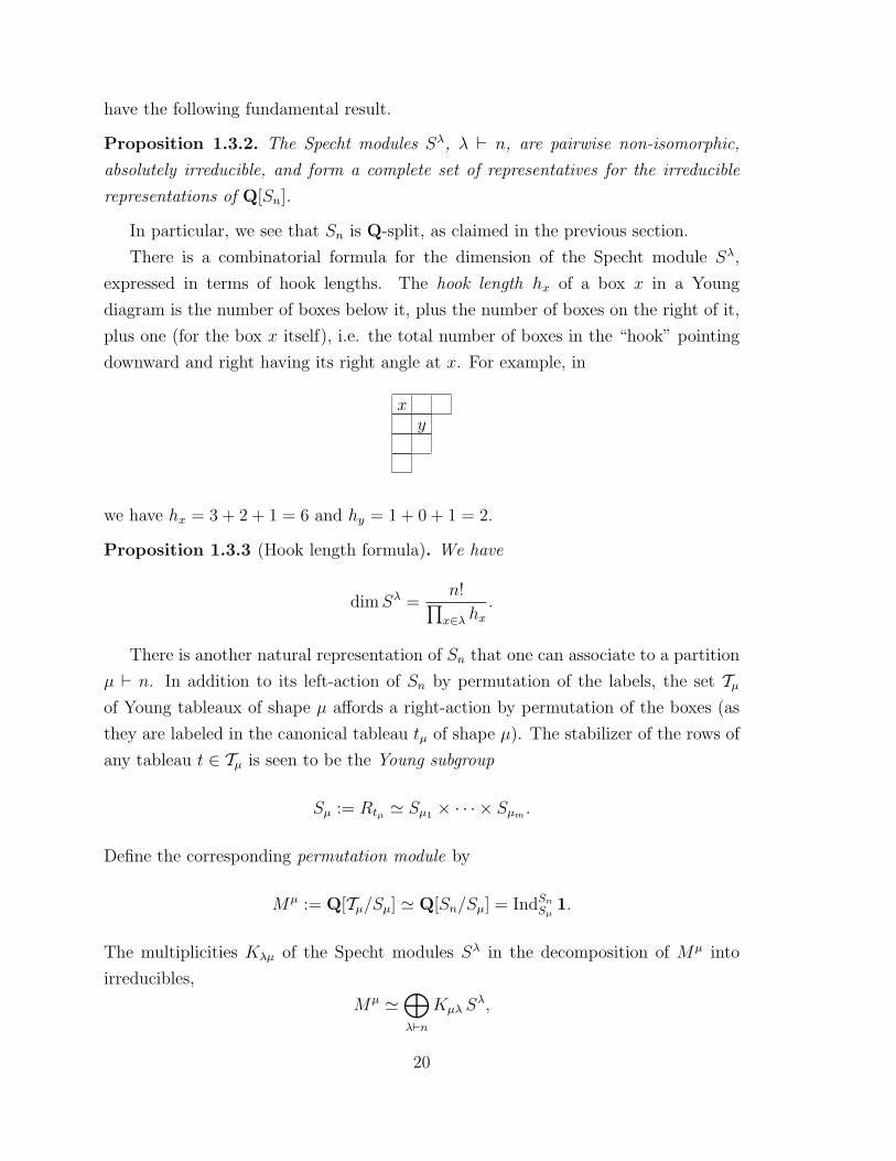
There is a combinatorial formula for the dimension of the Specht module Sλ,

expressed in terms of hook lengths. The hook length hx of a box x in a Young

diagram is the number of boxes below it, plus the number of boxes on the right of it,

plus one (for the box x itself), i.e. the total number of boxes in the “hook” pointing

downward and right having its right angle at x. For example, in

xy

we have hx = 3 + 2 + 1 = 6 and hy = 1 + 0 + 1 = 2.

Proposition 1.3.3 (Hook length formula). We have

dimSλ =n!∏x∈λ hx

.

There is another natural representation of Sn that one can associate to a partition

µ ` n. In addition to its left-action of Sn by permutation of the labels, the set Tµof Young tableaux of shape µ affords a right-action by permutation of the boxes (as

they are labeled in the canonical tableau tµ of shape µ). The stabilizer of the rows of

any tableau t ∈ Tµ is seen to be the Young subgroup

Sµ := Rtµ ' Sµ1 × · · · × Sµm .

Define the corresponding permutation module by

Mµ := Q[Tµ/Sµ] ' Q[Sn/Sµ] = IndSnSµ 1.

The multiplicities Kλµ of the Specht modules Sλ in the decomposition of Mµ into

irreducibles,

Mµ '⊕λ`n

Kµλ Sλ,

20

are called the Kostka numbers. It is possible to work out an explicitly basis of

HomSn(Sλ,Mµ) in terms of semistandard tableaux. Given two partitions λ and µ

of n, a Young tableau of shape λ and content µ is a tableau of shape λ in which the

boxes have been labeled with µi times the integer i. For example,

4 1 25 13 21

1 3 51 22 41

1 1 12 23 54

are 3 tableaux of shape λ = 3, 2, 2, 1 and content µ = 3, 2, 1, 1, 1. We say that

such a tableau is semistandard if its entries are non-decreasing along each row, and

strictly increasing along each column. In the examples above, only the third one is

semistandard.

Proposition 1.3.4. The Kostka number Kλµ is the number of semistandard Young

tableaux of shape λ and content µ.

In particular, we find that Kλλ = 1, since the only semistandard Young tableau

of shape and content λ is the one in which the ith line is filled with the integer i. A

necessary and sufficient condition for Sλ to appear in Mµ, i.e. to have Kλµ > 0, is

that λ dominates µ, that is,

λ1 + · · ·+ λi ≥ µ1 + · · ·+ µi for all i ≥ 1.

If λ dominates µ, we write λD µ, and λB µ if in addition λ 6= µ. It can be seen that

dominance is a partial ordering on the set of partitions. Moreover, it follows that the

permutation module Mµ decomposes as

Mµ ' Sµ ⊕⊕λBµ

Kλµ Sλ.

1.4 Galois representations

Of particular interest to us are linear representations of Galois groups of a number

field. Let K be a number field, i.e. a finite extension of Q. Recall that the Galois

group of a Galois extension L/K is the group Gal(L/K) of all field automorphisms of

21

L which fix K. In particular, the absolute Galois group of K is

GalK := Gal(K/K),

where K is an implicitly fixed algebraic closure of K.

For any Galois extension L/K, when have an identification as groups,

Gal(L/K) = lim←−L′/K

Gal(L′/K),

where L′ ranges over all finite Galois subextensions of L/K. If we consider that all the

finite groups Gal(L′/K) on the right-hand side carry the discrete topology, this iden-

tification defines a topology on Gal(L/K), the Krull topology, giving it the structure

of a profinite group. (Of course, if L/K is finite, the resulting topology on Gal(L/K)

is discrete.) The basic feature of this topology is the Galois correspondence, according

to which the closed subgroups of Gal(L/K) are precisely the subgroups of the form

Gal(L/L′), where L′ is a subextension of L/K. In particular, the continuous quotients

of Gal(L/K) are exactly the Galois groups Gal(L′/K) of the Galois subextensions L′

of L/K.

We have the following crucial fact, which allows one to think of any λ-adic Galois

representation as being integer-valued (remember that all our representations are

required to be continuous).

Proposition 1.4.1. Let Eλ be a finite extension of Q` with ring of integers Oλ,

endowed with the λ-adic topology. Any linear representation of Gal(L/K) on a finite-

dimensional vector space V over Eλ stabilizes a full Oλ-lattice.

Proof. The Galois group Gal(K/L), being profinite, is compact, hence so is its image

under a continuous homomorphism ρ : GalK → GL(V ). The result follows from the

fact that all maximal compact subgroups of GL(V ) ' GLn(Eλ) are conjugated to

GLn(Oλ).

Given a nonzero prime ideal p in the ring of integers OK of K, the Galois group

Gal(L/K) acts transitively on the prime ideals P of the ring of integers OL of L which

lie above p, i.e., such that P ⊇ pOL. For such a prime P, let

D(P/p) := σ ∈ Gal(L/K) | σ(P) = P

22

be its stabilizer, called the decomposition group at P/p. It can be identified with the

Galois group of the local extension LP/Kp.

Writing kp for the finite field OK/p and kP for OL/P, one has a short exact

sequence

1 −→ I(P/p) −→ D(P/p) −→ Gal(kP/kp) −→ 1, (1.2)

which defines the inertia group at P/p as

I(P/p) = σ ∈ D(P/p) | σ(x) ≡ x mod P, ∀x ∈ OL.

Note that for σ ∈ Gal(L/K),

D(σ(P)/p) = σD(P/p)σ−1 and I(σ(P)/p) = σI(P/p)σ−1. (1.3)

Definition 1.4.2. A homomorphism ρ : Gal(L/K)→ H is unramified at p if

I(P/p) ⊆ Ker ρ.

In particular, we say that the extension L/K is unramified at p if the identity homo-

morphism Id : Gal(L/K)→ Gal(L/K) is unramified at p, i.e. if I(P/p) = 1.

Note that, by (1.3), the definition does not depend on the choice of a prime P

above p.

Going back to the short exact sequence (1.2), we know that, since kp is a finite

field, the residual Galois group Gal(kP/kp) is topologically generated by the arithmetic

Frobenius substitution

x 7→ x|kp|,

or by its inverse, the geometric Frobenius substitution, which we denote Frob(P/p).

Now, if we assume that p is unramified in L, i.e. that I(P/p) = 1, then (1.2) becomes

just

D(P/p) ' Gal(kP/kp),

and we may think of Frob(P/p) as an element in the decomposition group D(P/p).

The Frobenius substitutions Frob(P/p) may change when the prime P above p varies,

but since Gal(L/K) acts transitively on these primes, and

Frob(σ(P)/p) = σ Frob(P/p)σ−1 for σ ∈ Gal(L/K),

23

we get a well-defined (geometric) Frobenius conjugacy class in Gal(L/K),

Frobp := Frob(P/p) | P divides pOL.

Theorem 1.4.3 (Weak Chebotarev). For a Galois extension L/K of a number field

K which is unramified outside a finite set of primes S, the Frobenius conjugacy classes

Frobp, p /∈ S,

are dense in Gal(L/K).

Given a finite set of primes S of K, let IS be the closed normal subgroup of

Gal(L/K) generated by all inertia subgroups I(P/p) for p /∈ S; then the quotient

Gal(L/K)S := Gal(L/K)/IS

is the largest continuous quotient of Gal(L/K) which is unramified outside S. By the

Galois correspondence, there exists a subextension LS of L/K such that

IS = Gal(L/LS);

it is the maximal subextension of L which is unramified outside S. More generally,

for any topological group H, the continuous homomorphisms ρ : Gal(L/K)→ H that

are unramified outside S are precisely those that factor through the quotient

Gal(L/K)S ' Gal(LS/K).

Proposition 1.4.4. Let E be a topological field and V a finite-dimensional vector

space over E, endowed with the product topology. Let ρ1 and ρ2 be two representations

of GalK into GL(V ) which are unramified outside S. Then

ρ1 ∼ ρ2 ⇐⇒ tr ρ1(Frobp) = tr ρ2(Frobp) for all p /∈ S.

Note that since the trace is constant on conjugacy classes, the right-hand statement

makes sense.

Proof. The equivalence class of a continuous representation of ρ : Gal(L/K)→ GL(V )

unramified outside S is determined by its trace, which we may view as a continuous

24

function on Gal(LS/K), and the trace is itself determined by its restriction to a dense

subset.

Definition 1.4.5. The Artin L-series of a Galois representation ρ : GalK → GL(V )

is the formal Dirichlet series on the monoid of non-zero ideals of OK given by the

formal Euler product

L(ρ, s) :=∏

p

det(1−N(p)sρ(Frobp) | V Ip)−1.

Even though this Dirichlet series converges for Re s > dimV when E = C, it

is important that we will always consider it here formally, in order to be able to

remember the individual Euler factors at the primes of K. In particular, if ρ1 and ρ2

are Galois representations with finite ramification, we have

ρ1 ∼ ρ2 ⇐⇒ L(ρ1) = L(ρ2) up to finitely many Euler factors.

The following is a crucially important example of `-adic Galois representation.

Example 1.4.6. For any prime integer `, GalK permutes the `th roots of unity µ`(K)

in the algebraic closure K, hence acts on

µ`∞(K) := lim←−n

µ`n(K) ' lim←−n

Z/`nZ = Z`.

Let ψ` denote the corresponding homomorphism

GalK −→ Autµ`∞(K) ' Z×` .

In other words, GalK acts on a root of unity ζ ∈ µ`∞(K) by

σ · ζ = ζψ`(σ).

In particular, for any prime p of K away from `, the arithmetic Frobenius Frob−1p acts

on `-power roots of unity by raising to the N(p), so that

ψ`(Frob−1p ) = N(p), (p, `) = 1.

The character ψ` could be called the arithmetic `-adic cyclotomic character of GalK ;

25

we will prefer to work instead with the geometric `-adic cyclotomic character

χ` := ψ−1` ,

so that we have

χ`(Frobp) = N(p), (p, `) = 1.

It is an `-adic 1-dimensional representation of GalK which is unramified away from `.

Note that its Artin L-function L(χ`, s) equals the Dirichlet zeta-function ζK(s) of K

up to the Euler factors corresponding to primes above `.

For i ∈ Z, and V an `-adic Galois representation, we will denote by V (i) the Galois

module structure on V obtained by tensoring (over Z`) by the ith power of the `-adic

cyclotomic character. This is called the ith Tate twist of V .

Another concept we will need to use (albeit somewhat informally) for `-adic rep-

resentations is that of Hodge-Tate weights (see e.g. [63] or [18, ch. 5]). Let C` denote

the `-adic completion of the algebraic closure of Q`, equipped with its natural Galois

action by GalQ`.

Definition 1.4.7. An n-dimensional `-adic Galois representation V is called Hodge-

Tate if we have a GalQ`-equivariant decomposition

C` ⊗Q`V ' C`(i1)⊕ · · · ⊕C`(in).

The integers HT(V ) = i1, . . . , in, with multiplicities, are then called the Hodge-Tate

weights of V .

In the language of Fontaine’s theory, Hodge-Tate representations are those which

are BHT-admissible, where BHT is the graded ring

BHT = C`[t, t−1] =

⊕i∈Z

C` ti =

⊕i∈Z

C`(i),

with GalQ`acting on t via the cyclotomic character.

We will content ourselves of noting the following facts from the “yoga of weights”.

• The cyclotomic character χ` is Hodge-Tate with weight 1.

26

• If ρ1 and ρ2 are Hodge-Tate, then ρ1 ⊕ ρ2 and ρ1 ⊗ ρ2 also are, with

HT(ρ1 ⊕ ρ2) = HT(ρ1) ∪ HT(ρ2),

HT(ρ1 ⊗ ρ2) = HT(ρ1) + HT(ρ2).

• If ρ is Hodge-Tate, then det ρ also is with single weight∑

HT(ρ).

1.5 Compatible systems

In addition to considering a single λ-adic Galois representation, it will be needed to

vary λ and consider families of representations satisfying a compatibility condition,

since this is how they arise “in nature” (i.e. from etale cohomology). One should think

of these different `-adic incarnations of a single, “motivic” object. We now formulate a

precise definition, which corresponds to what Serre calls “strictly compatible systems”

in [56]. Given K and E two number fields and λ a prime of E, let Sλ denote the set

of primes of K which divide N(λ).

Definition 1.5.1. An E-rational compatible system of λ-adic representations of de-

gree n of GalK is a family indexed by the finite places λ of E,

ρ = ρλ : GalK −→ GLn(Eλ)λ ,

for which there exists a finite set S of primes of K such that for every λ:

• ρλ is unramified outside S ∪ Sλ;

• for every prime p 6∈ S ∪ Sλ of K, the characteristic polynomial

det(1− t ρλ(Frobp)) ∈ Eλ[t]

has coefficients in E, and does not depend on λ.

The minimal set S satisfying these two conditions, the “exceptional set” of [56], will

be denoted Ram ρ.

Example 1.5.2. To any representation ρ : GalK → GLn(E) with finite ramification,

one can trivially associate a compatible system by putting

ρλ := ρ⊗ Eλ.

27

This defines a canonical inclusion of the category of finitely ramified E-representations

of degree n into the category of E-rational compatible systems of degree n.

This example, although seemingly innocent, is psychologically important because

compatible systems are precisely the families of λ-adic representations over the com-

pletions of E which look like they come from a single representation over E. Note

that here we think about the category of E-rational compatible systems as a full sub-

category of the product of the categories of Eλ-representations. We can thus make

sense in a natural way of all the operations on representations by performing them

component-wise.

Example 1.5.3. If ρ is an E-rational compatible system with finite ramification, then

det ρ is a 1-dimensional E-rational compatible system with Ram(det ρ) ⊆ Ram ρ.

Example 1.5.4. The cyclotomic character χcycl := (χ`)` is a Q-rational compatible

system of `-adic representations of GalK with Ramχcycl = ∅.

If ρ = (ρλ)λ is an E-rational compatible system of λ-adic representations, then

all the individual representations share the same Artin L-function at all unramified

primes, i.e. up to finitely many Euler factors, and we can consider this to be the

L-function attached to ρ. To be precise, we let

L(ρ, s) :=∏

p 6∈Ram ρ

det(1−N(p)s ρλ(Frobp))−1,

where the choice of λ away from p in the Euler factor at p is immaterial. If ρ is a com-

patible system of continuous λ-adic representations, L(ρ, s) completely characterizes

ρss, the semisimple compatible system associated to ρ.

Example 1.5.5. For the trivial representation 1 of GalK , considered as a compatible

system, we have

L(1, s) =∏

p

1

1−N(p)s= ζK(s),

the Dedekind zeta function of K.

Example 1.5.6. For the rth power of the cyclotomic character of K, we have

L(χrcycl, s) =∏

p

1

1−N(p)s+r= ζK(s+ r).

28

More generally, if ρ is any compatible system of representations of GalK , then for its

rth Tate twist ρ⊗ χrcycl we have

L(ρ⊗ χrcycl, s) = L(ρ, s+ r).

A very important family of 2-dimensional compatible systems are those attached

to modular forms by Deligne (see [46] for an exposition). A compatible system of

representations ρ = (ρλ)λ is said to have Hodge-Tate weights HT(ρ) if all the individual

λ-adic representations are Hodge-Tate with the same weights HT(ρλ) = HT(ρ).

Proposition 1.5.7. Let f be a Hecke newform of weight k, level N and Nebenty-

pus ε, i.e. f ∈ Snewk (N, ε), and let E = Q(f) be the number field generated by its

Fourier coefficients. There exists a 2-dimensional E-rational compatible system of

representations ρf of GalQ, with HT(ρf ) = 0, k− 1, unramified away from N , such

that

det ρf = ε⊗ χk−1cycl

and

tr ρf (Frobp) = ap(f), for all p - N.

In particular, the L-function L(ρf , s) is equal to the Mellin transform of f up to

Euler factors for p | N . Note that these factors are completely determined by those

for p | N by “multiplicity 1” for newforms.

29

30

Chapter 2

Etale cohomology

We will want to study in Chapter 4 the distribution of certain exponential sums via

their moments, which can in turn be expressed in terms of the number of points on

projective hypersurfaces defined by equations of the form

m∑i=1

xi =n∑j=1

yj,m∑i=1

xki =n∑j=1

ykj . (2.1)

As is often the case, this counting problem can be conveniently treated using etale

cohomology, and this chapter lays down the relevant facts to be used in the sequel.

We first describe in Section 2.1 the construction and some of the properties of the

λ-adic cohomology groups

H•(X,Fλ)

of a variety defined over a number field K with values in a λ-adic constructible

sheaf Fλ. If we let Fλ vary along a compatible system of λ-adic sheaves, the graded

Galois representations afforded by the cohomology groups form a compatible system

thanks to the Grothendieck trace formula (Section 2.2). In particular, if we take

sheaves with trivial Galois action by GalK , such as the various λ-adic completions of

a number field E, we recover the number of points of the reductions of X over finite

fields as the alternating trace of Frobenius morphisms on the cohomology.

The varieties defined by the equations (2.1) above are often smooth, but may be

singular in general. The singularities will be seen in the next chapter (Section 3.4) to

consist of isolated ordinary double points, i.e. points which become smooth quadrics

when blown-up. Accordingly, we proceed to discuss the cohomology of smooth hy-

persurfaces in Section 2.3, which is particularly simple since the Lefschetz hyperplane

31

theorem implies that only the middle-degree cohomology carries non-trivial informa-

tion. The special case of smooth quadrics in then described in some more details in

Section 2.4. In the last pages (Section 2.5), we describe the results of Schoen [49] about

the cohomology of singular hypersurfaces of odd dimension whose only singularities

are ordinary double points, and treat as well the case of even dimension.

2.1 Basic properties

In this section, we roughly describe how etale cohomology is defined, and then state

without any attempt of proof some of its formal properties. The reader is referred to

[23] for a quick overview, to [41] for a readable account, to [61, 19] for more details,

and of course to the SGA for the source, in particular [14].

Let F be an separably closed field, and X a scheme over F. As well as the category

XZar of Zariski open sets of X, one may consider with Grothendieck et al. the larger

category Xet of etale open sets of X, together with the natural “continuous” map

ι : Xet −→ XZar.

At the level of sheaves, ι induces an etalization map ι∗ : Sh(XZar)→ Sh(Xet). Since

the category Sh(Xet) of etale sheaves has enough injectives, sheaf cohomology, as the

right derived functor to the global sections, is defined. Hence, for any Zariski sheaf

F ∈ Sh(XZar), we can define the etale cohomology groups of X with values in F as

H•et(X,F) := H•(Xet, ι∗F).

Definition 2.1.1. Let Eλ be a local number field with ring of integers Oλ. A λ-adic

constructible sheaf on a topological space X is a constructible sheaf Fλ of Eλ-vector

spaces together with a co-filtration (Fλ,n)n≥1, where Fλ,n is a sheaf of Oλ/λn-modules

and

Fλ =(

lim←−n

Fλ,n)⊗Oλ Eλ.

We define the ith etale cohomology group of X with coefficients in Fλ as

H i(X,Fλ) :=(

lim←−n

H iet(X,Fλ,n)

)⊗Oλ Eλ,

32

and write H•(X,Fλ) for the graded vector space

H•(X,Fλ) =⊕i

H i(X,Fλ).

In the case where X is defined over a perfect field K, we define

H•(X,Fλ) := H•(XK ,Fλ|XK ),

where XK = X ⊗ K denotes the base-change of X to K. When Fλ is the constant

sheaf Eλ, we will refer to H•(X,Eλ) as the λ-adic cohomology of X.

Proposition 2.1.2 (Functoriality). A morphism f : X → Y of K-schemes induces

a natural map

f ∗ : H•(Y,Fλ) −→ H•(X, f ∗Fλ)

for any λ-adic constructible sheaf Fλ on Y .

In particular, if G is any group of scheme automorphisms of X and Fλ a G-

equivariant constructible sheaf on X (in the sense that g∗Fλ = Fλ for all g ∈ G), then

H•(X,Fλ) is naturally endowed with a linear action from G.

Note that when F is a sheaf on X, then F|XK is a GalK-equivariant sheaf on XK ,

so that

H•(X,F) = H•(X ⊗K,F ⊗K)

inherits a Galois action from GalK to which we will return in Section 2.2 below.

In addition to being well-behaved on the category of schemes, etale cohomology

shares a lot of formal properties with Betti cohomology.

Proposition 2.1.3 (Finiteness). If X is a scheme of finite type over a perfect field

and Fλ a λ-adic constructible sheaf on X, the etale cohomology groups

H i(X,Fλ)

vanish unless 0 ≤ i ≤ 2 dimX. If in addition X is proper, they all have finite

dimension as vector spaces over Eλ.

Proposition 2.1.4 (Poincare duality). If X is smooth and separated, there exists a

natural cup-product pairing

∪ : H i(X,Eλ)⊗Hj(X,Eλ) −→ H i+j(X,Eλ),

33

which is non-degenerate when i+ j = 2 dimX.

It is also true that etale cohomology agrees with Betti cohomology “as much as it

possibly could”.

Proposition 2.1.5 (Comparison theorem). If X is a smooth variety over a number

field, the choice of an embedding Eλ → C induces an isomorphism

H•(X,Eλ)⊗Eλ C ' H•Bet(X(C),C).

Recall that as a complex variety, we have a Hodge decomposition

H iBet(X(C),C) = H i

dR(X(C),C) =⊕p+q=i

Hp,q(X(C),C).

The comparison isomorphism also preserves the Hodge structures on both sides, in

the following sense. If we set

hp,q := dimHp,q(X(C),C) = dimHq(X(C),Ωp),

then hp,q is the multiplicity of p in HT(H i(X,Eλ)). In particular, since hp,q = hq,p,

we see that the multiset of Hodge-Tate weights of H i(X,Eλ) is invariant under the

involution p 7→ i− p.The following fact is also crucial to describe the residual Galois representations on

etale cohomology at primes of good reduction. Recall that the spectrum of a Henselian

discrete valuation ring (such as the ring of integers in a local number field) is called

a Henselian trait.

Proposition 2.1.6 (Smooth base change). Let X be a smooth proper scheme over a

Henselian trait with generic fiber X and special fiber Xp, and Fλ a λ-adic constructible

locally constant sheaf on X where λ is coprime with the characteristic of the base field.

Then the natural maps

H•(X,Fλ|X)←− H•(X ,Fλ) −→ H•(Xp,Fλ|Xp)

are isomorphisms.

In particular, let X be a smooth proper variety defined over a number field K and p

a prime of good reduction for X. This means that there exists a smooth proper model

34

X of X over SpecKp, which carries an action of the decomposition group Dp ⊆ GalK .

The functorial isomorphism given by smooth base change tells us that

H•(X,Fλ|X) ' H•(Xp,Fλ|Xp)

as representations for Dp. But the action on the right-hand side factors through the

residual Galois group Galkp , so we conclude that the inertia group Ip acts trivially on

the left-hand side as well. We conclude the following.

Corollary 2.1.7. If X is a smooth proper variety defined over a number field K, the

Galois representation of GalK on H•(X,Eλ) is unramified outside the primes of bad

reduction of X. In particular, it has finite ramification.

2.2 The trace formula and purity

Weil [65] remarked early on that an analogue of the Lefschetz trace formula for the

Frobenius automorphism of a variety defined over a finite field would be highly desir-

able, since it would allow to study the number of points of that variety using coho-

mological methods. Such a formula was proved first by Grothendieck in the version

that we state here, then later generalized by Verdier.

Theorem 2.2.1 (Trace formula). Let X be a smooth, proper variety over Fq and Fλa λ-adic constructible sheaf on X with λ away from q. For the geometric Frobenius

morphism Frobq, we have

∑x∈X(Fqr )

tr(Frobq | Fλ,x) =2 dimX∑i=0

(−1)i tr(Frobq | H i(X,Fλ)),

or, more concisely, considering the right-hand side as a trace in the graded sense:

tr(Frobq | Fλ,X(Fqr )) = tr(Frobq | H•(X,Fλ)).

Definition 2.2.2. Let X be a smooth, proper variety defined over Fq and Fλ a

constructible λ-adic sheaf. The zeta function of X with coefficients in Fλ is the

formal series

Z(X,Fλ; t) := exp

∞∑r=1

tr(Frobrq | Fλ,XF )tr

r

∈ Eλ[[t]].

35

In particular, when Fλ = Eλ, as Frobenius acts trivially on the stalks, we have

tr(Frobrq | Fλ,X(Fqr )) = |X(Fqr)|,

and the zeta function Z(X,Eλ; t) is just a generating series for the number of points

of X over all finite extensions Fqr of Fq.

Corollary 2.2.3. The zeta function of a smooth, proper variety X defined over Fq

with coefficients in Fλ can be written as

Z(X,Fλ; t) = det(1− tFrobq | H•(X,Fλ))−1.

In particular, it is a rational function of t with coefficients in Eλ.

Proof. If X is defined over Fq, then for any r ≥ 1 we may consider X as defined over

Fqr , and since Frobqr = Frobrq, the trace formula implies that

tr(Frobrq | Fλ,XF ) = tr(Frobrq | H•(X,Fλ)), r ≥ 1.

The conclusion follows by taking the exponential on both sides of the definition of the

zeta function and using Lemma 1.1.5.

Now suppose that X is a global variety defined over a number field K. By smooth

base change, for every prime p of good reduction for X, if Fλ is a λ-adic constructible

sheaf on X which extends to a smooth model X , we have

H•(X,Fλ) ' H•(Xp,Fλ|Xp)

as representations for the decomposition group Dp at p, so that

det(1− tFrobp | H•(X,Fλ)) = det(1− tFrobp | H•(Xp,Fλ)).

It follows that the (global) zeta function of X,

ζ(X,Fλ; s) := L(H•(X,Fλ), s),

defined as the Artin L-function (in the graded sense) of its etale cohomology viewed

36

as a representation for GalK , factors up to finitely many Euler factors as

ζ(X,Fλ, s) =∏

good p

Z(Xp,Fλ|Xp ;N(p)−s).

It is then natural to consider compatible families of λ-adic sheaves in order to

obtain a compatible system of λ-adic representations from etale cohomology.

Definition 2.2.4. A family F = (Fλ)λ of λ-adic constructible sheaves on X will be

called compatible if for all primes p of good reduction for X, the number

tr(Frobrp | Fλ,Xp(Fqr )) ∈ Eλ

actually lies in E and is independent on the choice of λ away from p.

In particular, if F is a constructible sheaf of E-vector spaces on X, then (F⊗Eλ)λis a compatible family of λ-adic sheaves on X which could still be denoted F by abuse

of notation. The following follows at once from the trace formula.

Corollary 2.2.5. Let X be a scheme of finite type over a perfect field K, E a number

field and F a compatible system of λ-adic constructible sheaves on X. Then

H•(X,F) :=(H•(X ⊗K,Fλ)

)λ

is a compatible system of graded λ-adic representations of GalK.

It should also be mentioned that Deligne, in his celebrated paper [13], completed

the proof of the Weil conjectures by proving the Riemann hypothesis for varieties over

finite fields.

Theorem 2.2.6 (Purity). Let X be a smooth proper variety over Fq and Fλ a λ-adic

constructible sheaf on X. If all the eigenvalues of Frobq on the stalks Fλ,x are pure of

weight a, i.e. have absolute value qa/2 under every embedding Eλ → C, then all the

eigenvalues of Frobq on H i(X,Fλ) are pure of weight a+ i.

In particular, if we take Fλ to be the constant sheaf Eλ, on which Frobenius acts

trivially hence purely of weight 0, then all the eigenvalues of Frobq on H i(X,Eλ) are

pure of weight i. One of the striking applications of purity is giving bounds on certain

exponential sums; more on this in Chapter 4.

37

2.3 Smooth hypersurfaces

This section is devoted to the cohomology of smooth projective hypersurfaces, both

from the geometric and Galois points of view. We start by describing the cohomology

of projective space, since the Lefschetz hyperplane theorem states that the cohomology

of a smooth hypersurface is almost the same as that of the ambient projective space.

Let X be a variety defined over a perfect field K and let CH•(X) denote its Chow

ring, i.e. CHi(X) is the free abelian group on the subvarieties (defined over K) of

X of codimension i, modulo linear equivalence, the product on the graded module

CH•(X) being given by

∩ : CHi(X)⊗ CHj(X) −→ CHi+j(X), [Z1] ∩ [Z2] = [Z1 ∩ Z2],

when Z1 and Z2 meet transversally.

Proposition 2.3.1 (Cycle class map). There exists a functorial homomorphism of

graded compatible systems of algebras given by

γ : CHi(X)(i) −→ H2i(X,Eλ).

Recall that the notation M(i) refers to the ith Tate twist of M (cf. Example 1.5.6).

In the case of projective space Pn, it is well known that

CHi(Pn) = 〈γ[H]i〉,

where H ' Pn−1 is any hyperplane, and that the cycle class map is actually a bijection

onto H•(Pn). Thus, as a graded compatible system,

H•(Pn) = χ0cycl 0 χ1

cycl 0 χ2cycl . . . 0 χncycl,

where χicycl is the action on H2i(Pn). This could also have been deduced from the fact

that over every finite field Fq,

|Pn(Fq)| =qn+1 − 1

q − 1= 1 + q + q2 + · · ·+ qn,

together with the trace formula.

Now suppose that X is a smooth hypersurface in Pn+1. The following result states

that the only interesting cohomology of X occurs in the middle degree n.

38

Proposition 2.3.2 (Lefschetz hyperplane theorem). If j denotes the inclusion of a

smooth hypersurface X in Pn+1, then

j∗ : H i(Pn+1) −→ H i(X)

is an isomorphism for i < n, and is injective for i = n.

Remark. From Poincare duality, it follows that j∗ is also an isomorphism above the

middle degree. Indeed, for n < i ≤ 2n, consider the following commutative diagram.

H i(Pn+1)

j∗

⊗H2n−i(Pn+1)

j∗'

∪ // H2n(Pn+1)

j∗'

H i(X)⊗

H2n−i(X)∪ // H2n(X)

The Lefschetz hyperplane theorem guarantees that j∗ is an isomorphism in degree

2n− i < n. Note that j∗ is known to be an isomorphism in degree 2n, since it maps

the generator γ[H]n of H2n(Pn+1), the class of a line, to degX points in H2n(X). It

then follows by taking duals that j∗ is an isomorphism in degree i as well.

In degree n, it is actually possible to define a canonical complement to j∗Hn(Pn+1),

the primitive cohomology Hnpr(X) of X, using the hard Lefschetz theorem. Of course,

if n is odd, there is nothing to do as Hn(Pn+1) = 0.

Corollary 2.3.3. If X is a smooth hypersurface of dimension n, we have

H•(X) ' H•(Pn)⊕Hnpr(X)

as graded compatible systems.

Proof. For i < n, by the Lefschetz hyperplane theorem, we have

H i(X) ' H i(Pn+1) ' H i(Pn),

i.e. 0 if i is odd and χi/2cycl if i is even. For i = n, we similarly have

Hn(X) = Hn(Pn+1)⊕Hnpr(X) ' Hn(Pn)⊕Hn

pr(X).

For i > n, by Poincare duality it follows that

H i(X) ' H2n−i(X)∨(n) = H2n−i(X)∨ ⊗ χncycl,

39

from which the conclusion follows.

It is possible, using the Riemann-Roch-Hirzebruch formula, to give a general for-

mula for the Hodge numbers of the primitive cohomology of a smooth complete in-

tersection over C ([24, app. 1] and [12]). In the case of smooth hypersurfaces, we

have the following. For p+ q = n, let hp,qd denote the Hodge numbers of the primitive

cohomology of a smooth hypersurface of degree d and dimension n, and let

Hd(x, y) :=∑p,q≥0

hp,qd xpyq.

Proposition 2.3.4. The generating series Hd(x, y) for the primitive Hodge numbers

of smooth hypersurfaces of degree d is

Hd(x, y) =(1 + x)d−1 − (1 + y)d−1

x(1 + y)d − y(1 + x)d.

In particular, evaluating this expression at x = y (and using the formal L’Hopital

rule for the right-hand side) yields the following formula for the dimension of the

primitive cohomology of smooth hypersurfaces.

Corollary 2.3.5. If X is a smooth hypersurface of degree d and dimension n, t hen

dimHnpr(X) =

(d− 1)n+2 + (−1)n(d− 1)

d.

For example, if n = 0, we find dimH0pr(X) = d− 1, as it should. Similarly, when

X is a smooth curve, we recover the classical degree-genus formula

dimH1(X) = 2

(d− 1

2

).

Moreover, if d = 1, so that X ' Pn is an hyperplane in Pn+1, the primitive cohomol-

ogy of X vanishes.

Recall that the Euler characteristic of X is defined in general by

χ(X) := tr(Id | H•(X)) =2 dimX∑i=0

(−1)i dimH i(X).

Corollary 2.3.6. The Euler characteristic of a smooth projective hypersurface X of

40

degree d and dimension n is given by

χ(X) = n+ 2 +(1− d)n+2 − 1

d.

Proof. This follows at once from Corollary 2.3.3, which implies that

χ(X) = χ(Pn) + (−1)n dimHpr(X) = n+ 1 + (−1)n dimHpr(X),

together with the formula of Corollary 2.3.5.

We now turn to a description of structure of Galois module afforded by the prim-

itive cohomology of a smooth hypersurface, which can in some situations be studied

by elementary means, a la Weil, using Gauss and Jacobi sums to count points on

the hypersurface. Recall that the Gauss sum associated to a multiplicative character

χ : F×q → C× of the finite field Fq of characteristic p is defined by

g(χ) :=∑x∈F×q

χ(x) exp

(2πi

ptrFq/Fp(x)

).

For the rest of this section, let X be the diagonal hypersurface in Pn−1 defined by

n∑i=1

aixki = 0. (2.2)

Provided k is invertible in the base field, X is smooth if and only if ai 6= 0 for all i.

Proposition 2.3.7 ( [26, §11.3, th. 2] ). Let X be the diagonal hypersurface (2.2) of

dimension n− 2 over the field Fq, with ai 6= 0, q ≡ 1 mod k. The zeta function of X

is given by

Z(X/Fq; t) =P (t)(−1)n+1

(1− t)(1− qt) · · · (1− qn−2t),

where P (t) is the polynomial

∏(1− (−1)n

q

n∏i=1

χi(a−1i )g(χi)t

),

the product ranging over all n-tuples (χ1, . . . , χn) of multiplicative characters of Fq

such that χki = 1, χi 6= 1 and χ1 · · ·χn = 1.

41

From Corollary 2.3.3, the polynomial P (t) appearing above is nothing but the

characteristic polynomial of Frobq on Hn−2pr (X). In particular, using the fact that

|g(χ)| = √q for any Gauss sum over Fq, we find that the eigenvalues of Frobenius on

the primitive cohomology have absolute value∣∣∣∣∣(−1)n

q

n∏i=1

χi(a−1i )g(χi)

∣∣∣∣∣ =1

q

n∏i=1

|χi(a−1i )||g(χi)| =

1

q

n∏i=1

q1/2 = q(n−2)/2,

in accordance with purity. (This was actually one of the examples which led Weil to

formulate his conjectures.)

The degree of P (t) is the number of n-tuples of characters (χ1, . . . , χn) appearing

in Proposition 2.3.7. For fixed number of variables n and degree k, let

Ωn,k := (χ1, . . . , χn) | χi ∈ F×q , χki = 1, χi 6= 1 and

Dn,k := (χ1, . . . , χn) ∈ Ωn,k | χ1 · · ·χn = 1.

As Ωn,k\Dn,k is in bijection with Dn+1,k via (χ1, . . . , χn) 7→ (χ1, . . . , χn, (χ1 · · ·χn)−1),

we have

|Ωn,k| = |Dn,k|+ |Ωn,k \Dn,k| = |Dn,k|+ |Dn+1,k|.

Since by assumption k divides the order of the cyclic group F×q , |Ωn,k| = (k − 1)n. It

follows that |Dn,k| satisfies the recurrence equation

|Dn+1,k| = (k − 1)n − |Dn,k|, n ≥ 1,

with initial condition |D1,k| = 0. By an easy induction argument, one finds that

|Dn,k| =(k − 1)n + (−1)n(k − 1)

k,

which is precisely the dimension of the primitive cohomology of X according to Propo-

sition 2.3.5.

2.4 Smooth quadrics

We now specialize the discussion of the previous section to smooth quadrics over

perfect fields. A projective quadric Q of dimension n in Pn+1 is defined by the

vanishing of a homogeneous quadratic polynomial f(x), which over a perfect field F

42

of characteristic different than 2 can be written as

f(x) = xtAx,

where A is a symmetric matrix with coefficients in F. Using Gauss-Lagrange reduction

on the matrix A, we can find an invertible matrix B such that

BtAB = diag(a1, . . . , an+2),

hence the quadric Q is projectively equivalent to the diagonal quadric

n+2∑i=1

aix2i = 0.

Since diagonal hypersurfaces are smooth if and only if none of their coefficients vanish,

it follows that Q is smooth if and only if

detA = (detB)2

n+2∏i=1

ai 6= 0.

Now, if Q is smooth, by Corollary 2.3.5, we have

dimHnpr(Q) =

1 + (−1)n

2=

0 for n odd,

1 for n even.

Hence, when n is odd, from Corollary 2.3.3 we have the following.

Proposition 2.4.1. If Q is a smooth quadric of odd dimension n, then

H•(Q) ' H•(Pn).

Now, if Q is a smooth quadric of even dimension, its primitive cohomology is 1-

dimensional and we will now determine explicitly the Galois representation it carries.

We first make a definition.

Definition 2.4.2. Let Q be a smooth quadric over F of dimension n = 2r defined by

the homogeneous equation xtAx, where A is a symmetric (n + 2) × (n + 2) matrix.

43

The signed discriminant of Q is defined to be

∆(Q) := (−1)r+1 detA ∈ F×/(F×)2.

Note that since the signed discriminant ∆(Q) is only considered modulo squares, it

does not depend on the choice of a matrix A and thus only depends on the projective

quadric Q.

Proposition 2.4.3. Let Q be a smooth quadric of even dimension n = 2r defined over

a finite field Fq of characteristic different from 2. Then Frobq acts on the primitive co-

homology Hnpr(Q) by multiplication by εq(∆) qr, where εq is the (unique) multiplicative

character of Fq of order 2, and ∆ = ∆(Q) is the signed discriminant of Q.

Proof. Without loss of generality, we can assume that Q is a diagonal quadric

n+2∑i=1

aix2i = 0.

By Proposition 2.3.7, Frobq acts on Hnpr(Q) by multiplication by

1

q

n+2∏i=1

χi(a−1i )g(χi),

where the sum is over all (n + 2)-tuples of characters χi such that χ2i = 1, χi 6= 1

and χ1 · · ·χn+2 = 1. It turns out that the only possibility is to have χi = εq for all i,

where εq is the unique multiplicative character of Fq of order 2. Hence the action of

Frobenius is via multiplication by

1

q

n+2∏i=1

εq(a−1i )g(εq) =

1

qεq(a1 · · · an+2)g(εq)

n+2,

since

a−11 · · · a−1

n+2 ≡ a1 · · · an+2 modulo squares.

But here g(εq)2 = g(εq)g(εq) = εq(−1)q, so that the above expression equals

1

qεq(a1 · · · an+2)εq(−1)r+1qr+1 = εq(∆)qr,

as announced.

44

Corollary 2.4.4. If Q is a smooth quadric of dimension n = 2r defined over a number

field K, the compatible system of `-adic Galois representations on Hnpr(Q) is

χrcycl ⊗ ε∆,

where ∆ is the signed discriminant of Q and ε∆ : GalK Gal(K(√

∆)/K) → ±1is the corresponding quadratic character.

Proof. According to Proposition 2.4.3, the action of Frobp agrees for all finite places

p of K away from 2. The conclusion follows by continuity.

We could also have obtained the same result by a more geometric method, using

the fact that in this situation, the cycle class map

χ : CHr(Q)(r) −→ Hn(Q)

is actually surjective, and that two r-planes R and R′ in Q are rationally equivalent

if and only if

dimR ∩R′ ≡ r mod 2,

where we convene that dim∅ = −1 (see [21]).

By standard manipulations on quadratic forms, a defining equation for Q can be

brought into diagonal form and the variables arbitrarily paired to get an equation of

the formr+1∑i=1

αi(x2i − βiy2

i ) = 0.

The two r-planes defined over L := K(√β0, . . . ,

√βr),

R± : xi +√βiyi = 0, i = 0, . . . , r, xr+1 ±

√βiyi = 0,

yield different cohomology classes, and we have

Hn(Q) = 〈γ[R+], γ[R−]〉.

Now if√βi 6∈ K, the Galois involution

√βi 7→ −

√βi interchanges [R+] and [R−],

so that Gal(L/K) acts on [R+]+ [R−] trivially and on [R+]− [R−] as Gal(K(√

∆)/K)

because

detQ =r∏i=0

αi · (−αiβi) ≡ (−1)r+1

r∏i=0

βi mod (K×)2.

45

It follows after twisting by χrcycl that GalK acts via χrcycl(1⊕ ε∆) on

Hn(Q) = 〈γ[R+] + γ[R−]〉 ⊕ 〈γ[R+]− γ[R−]〉,

hence the action on Hnpr(Q) = 〈γ[R+]− γ[R−]〉 is via χrcycl ⊗ ε∆.

2.5 Hypersurfaces with ordinary double points

In this section we describe the cohomology of the desingularizations of hypersurfaces

whose singular locus consists only of ordinary double points, following and expanding

on Schoen’s treatment [49], where only hypersurfaces of odd dimension are considered.

Definition 2.5.1. A singular point x on a projective hypersurface X is an ordinary

double point if the tangent cone Cx(X) at x is a smooth quadric.

Let X a projective hypersurface of dimension m sitting inside P := Pm+1. We

suppose that the singular locus S of X consists entirely of ordinary double points.

Consider X → X (resp. P→ P) the blow-up of X (resp. P) along S.

The following is an analogue of the Lefschetz hyperplane theorem for the inclusion

j : X → P.

Proposition 2.5.2. The induced homomorphism in cohomology j∗ : H i(P)→ H i(X)

is an isomorphism for i ≤ m− 2, and injective for i ≤ m.

For convenient reference, we first state a standard fact from commutative algebra

that will be used in the proof.

Lemma 2.5.3 (Five lemma). Consider the following commutative diagram, in which

the rows are exact.

A1//

α

B1//

β

C1//

γ

D1//

δ

E1

ε

A2

// B2// C2

// D2// E2

1. If α is surjective, β and δ injective, then γ is injective.

2. If ε is injective, β and δ surjective, then γ is surjective.

In particular, if α, β, δ and ε are isomorphisms, then γ also is.

46

Proof of proposition. Let Q (resp. E) be the exceptional fiber in X (resp. P). By the

assumption that S consists only of ordinary double points, we have decompositions

Q = ts∈SQs, E = ts∈SEs, where Qs is a smooth quadric in Es ' Pm. By the

Lefschetz hyperplane theorem applied to the fibers Qs, the map

H i(E) =⊕s∈S

H i(Es) −→⊕s∈S

H i(Qs) = H i(Q)

is an isomorphism for i 6= dimQ = m− 1, and injective when i = m− 1.

Now consider the long exact sequences for the couples (X,S) and (P, S).

· · · // H i−1(P) //

H i−1(S) // H i(P, S) //

H i(P) //

H i(S) // · · ·

· · · // H i−1(X) // H i−1(S) // H i(X,S) // H i(X) // H i(S) // · · ·

Together with the Lefschetz hyperplane theorem for X → P, the five lemma implies

that H i(P, S)→ H i(X,S) is bijective for i < m and injective when i = m. The same

statement holds for H i(P, E)→ H i(X,Q) since the blow-ups induce isomorphisms

H i(P, E) // H i(X,Q)

H i(P, S) //

'OO

H i(X,S).

'OO

Now we may consider the long exact sequences associated to the couples (X,Q)

and (P, E).

· · · // H i−1(E) //

H i(P, E) //

H i(P) //

j∗

H i(E) //

H i+1(P, E) //

· · ·

· · · // H i−1(Q) // H i(X,Q) // H i(X) // H i(Q) // H i+1(X,Q) // · · ·

For i ≤ m−2, all vertical arrows besides j∗ are isomorphisms, hence by the five lemma

j∗ is an isomorphism as well. When i = m−1, H i−1(E)→ H i−1(Q) is an isomorphism

and H i(P, E) → H i(X,Q), H i(E) → H i(Q) are isomorphisms, which is enough to

apply the first part of the five lemma to conclude that j∗ is injective. For i = m, we

know that H i(P, E)→ H i(X,Q) is injective and H i(E)→ H i(Q) is an isomorphism.

However, in order to apply the five lemma to show that j∗ is injective, we need to

47

know that H i−1(E)→ H i−1(Q) is surjective, and this is the case only when m is even,

so that Q has no primitive cohomology (and actually H i−1(E) = H i−1(Q) = 0). For

m odd, one needs a slightly different argument as in [49] – again using the fact that

the connected components of Q are smooth quadrics.

Definition 2.5.4. Let us call

Hpr(X) := Hm(X)/Hm(P) and Hsub(X) := Hm−1(X)/Hm−1(P)

the primitive and subprimitive cohomology groups of X, respectively.

The following tells us that the subprimitive cohomology of X comes from the

primitive cohomology of the fibers of Q.

Proposition 2.5.5 ([49]). When m = dimX is even, Hsub(X) = 0. For m odd, let

k = m−12

and for every s ∈ S let Rs and R′s be two k-planes in Qs belonging to different

rulings, so that Hm−1pr (Qs) = 〈[Rs]− [R′s]〉. The cup-product induces an isomorphism

Hsub(X)∼−→ Hm+1

0 (X),

where Hm+10 (X) denotes the subspace of Hm+1(X) spanned by the classes [Rs]− [R′s],

for s ∈ S. Moreover, there is a natural isomorphism

Hm+10 (X)⊗C

∼−→ H1(P, IS ⊗K ⊗O(kX)).

We also need to understand the cohomology of P.

Proposition 2.5.6. Let P be the blow-up of P = Pm+1 along a finite set of points S,

and let E be the exceptional fiber. Then H i(P) = 0 when i is odd, and for 0 < i < m+1

we have a natural short exact sequence

0 −→ H2i(P) −→ H2i(P) −→ H2i(E) −→ 0.

Proof. Consider the long exact sequences associated to the couples (P, E) and (P, S).

· · · // H i−1(E) // H i(P, E) // H i(P) // H i(E) // H i+1(P, E) // · · ·

· · · // H i−1(S) //

OO

H i(P, S) //

'OO

H i(P) //

OO

H i(S) //

OO

H i+1(P, S) //

'OO

· · ·

48

Since S has dimension 0, from the lower line we see that H i(P, S) ' H i(P) for

all i. Hence, for i odd, since H i(P, E) ' H i(P) = 0 and H i(E) = 0, from the upper

line we conclude that H i(P) = 0. Similarly, when i > 0 is even, since H i−1(E) and

H i+1(P, E) ' H i+1(P) vanish, we get a short exact sequence

0 −→ H i(P, E) −→ H i(P) −→ H i(E) −→ 0,

in which we can replace H i(P, E) by H i(P).

We can get some information about the dimensions of the primitive and subprim-

itive cohomology using the Euler characteristic of X.

Proposition 2.5.7.

dimHpr(X) =

(d−1)m+2−1

d− |S| when m is even,

2 dimHsub(X) + (d−1)m+2+1d

− 2|S| when m is odd.

Proof. By Proposition 2.5.2 and Poincare duality,

χ(X) = χ(P) + 2(−1)m−1 dimHsub(X) + (−1)m dimHpr(X).

From Proposition 2.5.6, we see that

χ(P) = χ(P) + χ(E)− dimH0(E) = m+ 2 + |S|m− |S|,

since E ' ts∈SPm−1. But the Euler characteristic of X (see [38, Prop. 3.1], general-

izing Corollary 2.3.6) can be expressed as

χ(X) = m+ 2 +(1− d)m+2 − 1

d+ |S|(m+ δm),

where δm = 1 when m is odd, and δm = −2 when m is even. Comparing the two

expressions for χ(X) yields

dimHpr(X)− 2 dimHsub(X) =(d− 1)m+2 − (−1)m

d+ (−1)m|S|(δm + 1),

from which the conclusion follows according to the parity of m.

Galois representations. Suppose now that our base algebraically closed field F

is separably closed and that the variety X is defined over a subfield K of which F

49

is the algebraic closure, so that H•(X) admits a natural action by GalK . Since all

the homomorphisms considered above are natural, they are Galois-equivariant when

it makes sense, so that they provide some information on H•(X) as a Galois module

as well.

By the Jacobian criterion, the singular locus S of X is defined over K, even though

the individual singular points need not. For a singular point s ∈ S, let K(s) be the

normal closure of the field of definition of s. Furthermore, let K(S) be the compositum

of all the extensions K(s), s ∈ S, so that S becomes isomorphic to |S| points over

K(S). The smooth quadric Qs above s ∈ S is easily seen to be defined over K(s) as

well.

The action of GalK on H•(Q) can be described as follows. Over K(S), Q is

isomorphic to ts∈SQs, so that

H•(Q) =⊕s∈S

H•(Qs)

as GalK(S)-modules, while Gal(K(S)/K) permutes the fibers among themselves. More

precisely, if we decompose S = tSi into disjoint GalK-orbits, each orbit Si is defined

over K, hence a corresponding decomposition Q = tQi over K. Choosing some point

si ∈ Si, we see that

H•(Qi) ' H0(Si)⊗H•(Qsi),

where Gal(K(si)/K) acts on H0(Si) by permuting the points and GK(si) acts on

H•(Qsi) as described in Section 2.4.

50

Chapter 3

Hypersurfaces with symmetries

When X is a variety defined over a number field K admitting an action by a finite

group G of K-automorphisms, its etale cohomology inherits an action of G commuting

with the Galois structure. The G-isotypic components of H•(X) are thus preserved

by the Galois action, and we prove in Section 3.1 that these isotypic components form

compatible systems of Galois representations. This fact could have been deduced by

suitably interpreting the work of Grothendieck [22] on the G-equivariant L-functions

defined in [51]. There, rationality results where obtained by interpreting every indi-

vidual element g ∈ G as a Frobenius morphism with respect to some twisted Galois

structure on X. The approach used here however is novel in that it gives a geometri-

cal (and, in this writer’s opinion, more natural) “motivic” explanation for rationality

by interpreting the multiplicity spaces of Section 1.2 as the etale cohomology groups

of the quotient X/G with coefficients in a suitable sheaf. Decomposing the trace

of Frobenius according to isotypic components (as will be done on certain examples

in Section 5.7) could not be carried out without the previous knowledge that these

systems of isotypic Galois representations are actually compatible.

The remainder of the chapter is devoted to the study of certain families of hyper-

surfaces admitting an action by the symmetric group Sn and for which the character

of the representation on primitive cohomology can be computed in a general fashion.

In Section 3.2 we define two such families, Sn-hypersurfaces of type I or II, and the

notion of a special Sn-hypersurface for which we can give a general formula for the

character of the representation of Sn on primitive cohomology (Theorem 3.2.14) by

using the Lefschetz fixed point theorem to relate the value of this character to the

Euler-Poincare characteristic of the fixed loci. We then discuss in Section 3.3 the exis-

tence of these special Sn-hypersurfaces, by providing some examples as well as certain

51

obstructions coming from the representation theory of Sn. A precise conjecture is

formulated about the existence of special hypersurfaces of type II.

In Section 3.4, we introduce and discuss the varieties Wm,n` , which arise naturally

when considering the moments of the exponential sums of Chapter 4 (the case ` = 2,

m = 0 was previously considered by Livne [38]). These varieties admit an action by

Sm×Sn; in particular, when m = 0, they are examples of Sn-hypersurfaces of type II

provided they are smooth. We thus discuss for which values of the parameters `,m, n

they are smooth, and prove that in any case their singularities are ordinary double

points, so that the cohomology of their desingularization can be studied via the results

of Section 2.5.

Finally, we perform in Section 3.5 some explicit computations of decomposition

into irreducibles of the corresponding representations for small values of the pa-

rameters. In particular, we observe that the primitive cohomology of W 0,72 admits

an isotypic component of dimension 2; the modular form corresponding to this 2-

dimensional compatible system will be explicitly determined in Chapter 5. We also

provided a description of the action of Sm × Sn on the subprimitive cohomology of

the desingularization of Wm,n` which will be needed to compute the moments of the

corresponding exponential sums in Chapter 4.

3.1 Isotypic decomposition

Let X be a smooth, proper variety defined over a number field K, on which a finite

group G acts by automorphisms defined over K. The goal of this section is to show

that the etale cohomology of X admits a G-isotypic decomposition

H•(X) =⊕φ

Mφ(H•(X))⊗Wφ, Mφ(H•(X)) = HomG(Wφ, H•(X)),

in the category of compatible systems. Recalling how etale cohomology is defined (Sec-

tion 2.1), we first prove the corresponding statement for sheaf cohomology, allowing

general sheaves of coefficients.

Suppose that X is a topological space on which a group G acts continuously on

the right.

Definition 3.1.1. A G-sheaf on X is a sheaf of finite dimensional vector spaces over

a field E of characteristic 0, endowed with a lift of the action of G on X, i.e. a couple

52

(F , θ), where F is a sheaf of E-vector spaces on X, and θ = (θg)g∈G is a collection of

isomorphisms θg : F → g∗F satisfying the cocycle relation

θgh = g∗θh θg, g, h ∈ G.

In particular, if G acts trivially on X, then a G-sheaf F on X is a “sheaf-valued

representation of G”, i.e. G acts on F by sheaf automorphisms. Using the notation

of Section 1.2, we can prove an isotypic decomposition for such sheaf-valued represen-

tations.

Lemma 3.1.2. Let F be a G-sheaf on X, where G is a finite group acting trivially

on X. There is a natural isomorphism

F =⊕

φ∈IrrE(G)

Mφ(F)⊗Eφ Wφ,

where Mφ(F) := HomG(Wφ,F) is the multiplicity sheaf of φ in F , and Wφ is con-

sidered as a constant sheaf.

Proof. As in the proof of Corollary 1.2.2, we have a natural homomorphism⊕φ∈IrrE(G)

Mφ(F)⊗Eφ Wφ −→ F

induced by the evaluation maps. To prove that it is an isomorphism of sheaves, it

suffices to check that it induces isomorphisms at the level of stalks. But for x ∈ X,

since

Mφ(F)x = HomG(Wφ,F)x = HomG(Wφ,Fx),

the induced map on the stalks at x is precisely the isotypic decomposition of Fx.

In general, if F is a G-sheaf on X, the sheaf cohomology H•(X,F) with coefficients

in F inherits by functoriality the structure of a graded E-valued representation for G.

As such, we can consider its isotypic decomposition

H•(X,F) =⊕

φ∈IrrE(G)

Mφ(H•(X,F))⊗Eφ Wφ. (3.1)

The following theorem says that the multiplicity spaces Mφ(H•(X,F)) can be in-

terpreted as the sheaf cohomology of the quotient X/G with values in the multiplicity

sheaves of the push-forward of F on X/G.

53

Theorem 3.1.3. Let G be a finite group acting on X and π : X X/G denote the

projection on the quotient. For any G-sheaf F on X, there is canonical isomorphism

Mφ(H•(X,F)) = H•(X/G,Mφ(π∗F)).

Proof. Since G is a finite group, π is a proper, finite map and thus induces an isomor-

phism

π∗ : H•(X/G, π∗F)∼−→ H•(X,F). (3.2)

Now π∗F is a G-sheaf on X/G, with G acting trivially on X/G, hence using

Lemma 3.1.2 we can write

π∗F =⊕

φ∈IrrE(G)

Mφ(π∗F)⊗Eφ Wφ.

Taking sheaf cohomology on both sides we obtain

H•(X/G, π∗F) =⊕

φ∈IrrE(G)

H•(X/G,Mφ(π∗F))⊗Eφ Wφ.

Comparing this expression with the isotypic decomposition (3.1) of H•(X,F) via the

isomorphism (3.2), we see that the assertion of the theorem would follow automatically

from the existence of a natural map

H•(X/G,Mφ(π∗F)) −→Mφ(H•(X,F)) (3.3)

since it would then automatically be an isomorphism. Now remark that

Mφ(π∗F)) = HomG(Wφ, π∗F) = Hom(Wφ, π∗F)G

naturally injects into Hom(Wφ, π∗F), hence the existence of a natural map

H•(X/G,Mφ(π∗F) −→ H•(X/G,Hom(Wφ, π∗F)),

which actually restricts, since G acts trivially on the left-hand side, to a map

H•(X/G,Mφ(π∗F)) −→ H•(X/G,Hom(Wφ, π∗F))G. (3.4)

54

Since Wφ is a constant sheaf, the functor Hom(Wφ,−) is exact, hence

H•(X/G,Hom(Wφ, π∗F))G = Hom(Wφ, H•(X/G, π∗F))G

= HomG(Wφ, H•(X/G, π∗F))

= Mφ(H•(X/G, π∗F))

= Mφ(H•(X,F)),

where we have used the isomorphism (3.2) again in the last step. It follows that (3.4)

gives the natural map (3.3) we were looking for, hence completing the proof.

It is reasonable to expect that such a result still holds in `-adic cohomology (at

least when the order of G is prime to `). Some details need to be supplied, since the

definition of `-adic cohomology is more involved than sheaf cohomology on ordinary

topological spaces; however, we will take this for granted here.

We can now state the desired result for arithmetic varieties. Recall that for a

scheme X on which a group G acts, a sufficient condition for the existence of the

quotient X/G in the category of schemes is that X can be covered by G-stable affine

sets [43, §7]. In such a case, writing X = ∪iUi as a union of G-stable open affine sets,

we can then construct X/G by gluing together the affine quotients Ui/G, where

Ui/G := SpecAGi if Ui = SpecAi.

Theorem 3.1.4. Let X be a smooth, proper variety defined over a number field K

and G a finite group acting on X by K-automorphisms such that the quotient X/G

exists and is smooth. Let F = (Fλ)λ be a λ-adic compatible system of constructible

G-sheaves over a number field E. The multiplicity

Mφ(H•(X,F))

in H•(X,F) of every irreducible representation φ ∈ IrrE(G) forms an E-rational

compatible system of λ-adic representations of GalK.

Proof. For every λ, it follows from the analogue of Theorem 3.1.3 that

Mφ(H•(X,Fλ)) = H•(X/G,Mφ(π∗Fλ))

as λ-adic representations of GalK . Since the quotient map π : X X/G is defined

55

over K, the push-forward sheaves π∗Fλ are seen to form a compatible family, and so

do the multiplicity sheaves Mφ(π∗Fλ) = HomG(Wφ, π∗Fλ).

Remark. The properness hypothesis on X/G, as well as on X, can be removed if one

is willing to use etale cohomology with compact support since the trace formula holds

in this context. Namely, it can be proven by exercising a little extra care that for any

compatible system F of λ-adic G-sheaves,

Mφ(H•c (X,F)) = H•c (X/G,Mφ(π∗F))

as compatible systems of λ-adic representations.

It follows immediately from the theorem that for a compatible system F of E-

rational λ-adic G-sheaves on X, we have an isotypic decomposition

H•(X,F) =⊕

φ∈IrrE(G)

Mφ(H•(X,F))⊗Eφ Wφ

as compatible systems of λ-adic Galois representations. As a result, if ζ(X,F) de-

notes the zeta function of H•(X,F) and ζφ(X,F) that of Mφ(H•(X,F)), we obtain

a factorization

ζ(X,F) =∏

φ∈IrrE(G)

ζφ(X,F)dimEφWφ =

∏φ∈IrrE(G)

ζ(X/G,Mφ(π∗F))dimEφWφ .

3.2 Symmetric hypersurfaces

The goal of this section is to compute the character of Sn acting on the cohomology

of certain kinds of symmetric projective hypersurfaces. Throughout, we fix n ≥ 1 a

positive integer and F an algebraically closed field in which n! 6= 0. We consider the

projective right action of the symmetric group Sn on the projective space Pn−1 by

permutation of homogeneous coordinates, i.e.

σ · [x1 : · · · : xn] := [xσ(1) : · · · : xσ(n)], σ ∈ Sn.

This is nothing but the projectivization of (the transpose of) the standard linear

permutation representation, i.e. the composition

Sn −→ GLn(F) PGLn(F) = Aut Pn−1.

56

We will consider two types of symmetric hypersurfaces.

Definition 3.2.1. An Sn-hypersurface of type I is a smooth hypersurfaceX ⊆ Pn−1 of

dimension n−2 which is stable under the action of Sn by permutation of homogeneous

coordinates. Let H be the hyperplane of Pn−1 defined by x1 + · · ·+ xn = 0.

An Sn-hypersurface of type II is a smooth projective hypersurface X ⊆ H of

dimension n− 3 which is stable under the action of Sn.

The hyperplane H ⊆ Pn−2 is itself a Sn-hypersurface of type I. Note that the action

of Sn on H can be thought of as the projectivization of the irreducible representation

of degree n− 1 occurring in the permutation representation on Fn.

We would like to compute in some generality the representation of Sn acting on

the cohomology of Sn-hypersurfaces of type I or II. In both cases the only interesting

part is the primitive cohomology thanks to the Lefschetz hyperplane theorem.

Proposition 3.2.2. Let X be a smooth projective hypersurface which is stable under

a group G of projective transformations. Then G acts trivially on the non-primitive

part of H•(X), and the character χpr of the representation on Hpr(X) is given for

g ∈ G by

χpr(g) = (−1)dimX

(χ(Fix g|X)− dimX − 1

),

where χ(Fix g|X) denotes the Euler characteristic of the fixed locus of g on X.

Proof. We first remark that the induced action of G on the cohomology of the ambient

projective space P is trivial, since H•(P) is generated by the class of a hyperplane,

and that any two hyperplanes are rationally equivalent. Hence, by the hard Lef-

schetz theorem, G acts trivially on the non-primitive part of H•(X). Now the graded

character χ• of G acting on H•(X) can be written as

χ• = χ(PdimX) + (−1)dimXχpr,

so that

χpr = (−1)dimX(χ• − χ(PdimX)

)= (−1)dimX

(χ• − dimX − 1

).

According to the Lefschetz fixed point formula (see [42, 33] and [15] in the algebraic

setting), for every g ∈ G we have

χ•(g) = tr(g∗ | H•(X)) = χ(Fix g|X),

57

which completes the proof.

In order to study the fixed loci of permutations on symmetric hypersurfaces, let

us first describe the fixed locus Fixσ in Pn−1 of a permutation σ ∈ Sn. First, note

that for a point [x] ∈ Fixσ, we have σ · x = αx for some scalar α ∈ F× which does

not depend on the choice of a representative x for [x]. Hence there is a partition of

the fixed locus as

Fixσ =⊔α∈F×

Fixα σ, where Fixα σ := [x] ∈ Pn−1 | σ · x = αx.

Note that a fixed point [x] ∈ Pn−1 for σ corresponds to a 1-dimensional linear repre-

sentation of the cyclic group 〈σ〉. It follows that if σm = 1, then Fixα σ = ∅ unless

αm = 1, so that we can restrict the disjoint union above to a finite number of roots

of unity in F.

Recall that any representation σ ∈ Sn can be written as a product of disjoint cycles

σ1, . . . σm, one for each orbit of 〈σ〉 on the set 1, . . . , n, and that this decomposition

is unique up to the ordering of these cycles. We shall refer to the set σ1, . . . , σmas the cycle decomposition of σ. Associated to this cycle decomposition is a partition

λ(σ) = λ1, . . . , λm of n, where λi denotes the length of the cycle σi. This partition

characterizes the conjugacy class of σ (cf. Section 1.3).

Definition 3.2.3. For a permutation σ ∈ Sn and any integer d ≥ 1, we define md(σ)

to be the number of parts in λ(σ) which are divisible by d.

Example 3.2.4. If σ = (12)(3456)(789) ∈ S10, then m1(σ) = 4, m2(σ) = 2, m3(σ) =

m4(σ) = 1, and md(σ) = 0 for d > 4.

Remark that for any permutation σ ∈ Sn, m1(σ) is just the number of cycles in

its cycle decomposition, while we necessarily have md(σ) = 0 for d > n.

Proposition 3.2.5. For σ ∈ Sn and α ∈ F× a scalar with multiplicative order d,

Fixα σ is a linear subspace of Pn−1 of dimension md(σ)− 1.

Proof. Write λ(σ) = λ1, . . . , λm. Since the statement only depends on the conjugacy

class of σ, we can assume that σ lies in Sλ1× . . .×Sλm under the standard embedding.

Any point x ∈ Fn can thus be written as x = (x1, . . . ,xm), with xi ∈ Fλi , and the

condition that σ · x = αx is equivalent to

σi · xi = αxi, i = 1, . . . ,m.

58

But as a linear transformation, σi has characteristic polynomial tλi − 1, so that the

above admits a non-zero solution xi if and only if αλi = 1, i.e. if and only if d | λi.Since tλi − 1 has distinct roots in F by our assumption on the characteristic of the

field, in the case where αλi = 1, the associated eigenspace of σi is 1-dimensional. Let

zλi(α) be an eigenvector of σi associated to α. Then we proved that the points in

Fixα σ are those of the form

[x1zλ1(α) : · · · : xnzλm(α)],

with x1, . . . , xm not all zero but xi = 0 if d - λi, which form a linear subspace of Pn−1

with md(σ) homogeneous coordinates.

This means that in the decomposition

Fixσ =⊔α∈F×

Fixα σ, (3.5)

we have Fixα σ ' Pmd(σ)−1 when O(α) = d. In particular, Fixα σ 6= ∅ if and only

if md(σ) > 0. Note that for composite d this is strictly stronger than the condition

mentioned earlier (σd = 1), since the order of σ is the least common multiple of

λ1, . . . , λm.

Lemma 3.2.6. For σ ∈ Sn, ∑d≥1

ϕ(d)md(σ) = n,

where ϕ is the Euler totient function.

Proof. From (3.5) and the additivity of the Euler characteristic, we find

χ(Fixσ) =∑d≥1

ϕ(d)χ(Pmd(σ)−1) =∑d≥1

ϕ(d)md(σ).

Since σ acts trivially on H•(Pn−1), the Lefschetz fixed point formula for σ reads

χ(Fixσ) = χ(Pn−1) = n,

and the result follows.

59

Note that this identity could also easily have been obtained by an elementary

argument by writing σ as a product of disjoint cycles.

We now turn to an explicit description of the two types of symmetric hypersurfaces

we are considering. We first state a standard lemma in the theory of symmetric

polynomials.

Lemma 3.2.7. Let ∆ :=∏

i<j(xi−xj) ∈ F[x1, . . . , xn] be the discriminant polynomial.

The vector space of polynomials where Sn acts via the alternating representation is

F[x1, . . . , xn]sg = ∆ · F[x1, . . . , xn]Sn .

Proof. As Sn acts on ∆ via sg, it is clear that ∆ ·F[x1, . . . , xn]Sn lies in F[x1, . . . , xn]sg.

To prove the reverse inclusion, let f be a polynomial such that σ · f = sg(σ)f for all

σ ∈ Sn. In particular, for i < j, we have (i j) · f = −f , hence

2f(x1, . . . , xi, . . . , xi, . . . , xn) = 0.

If there exists such a pair i < j, then necessarily n ≥ 2, so that by our hypothesis on

the characteristic, 2 is invertible in F. We conclude that f , considered as a polynomial

in xj with coefficients in the ring F[x1, . . . , xj, . . . , xn], has a root at xj = xi, hence

can be factored as f = (xi − xj)fij. If k < ` is another pair of indices, distinct (but

not necessarily disjoint) from (i, j), the same argument shows that f has a root at

x` = xk. However, since in all cases xi − xj does not vanish at x` = xk, we conclude

that fij has to be divisible by xk − x`. Continuing in this fashion, we find that f can

be written as

f =∏i<j

(xi − xj) · g = ∆ · g,

where g is some polynomial. But

σ · g = σ ·(f

∆

)=σ · fσ ·∆

=sg(σ)f

sg(σ)∆=f

∆= g,

so that g in invariant under the action of Sn as claimed.

Proposition 3.2.8. For n ≥ 3, any Sn-hypersurface of type I is of the form Z(f)

where f is a homogeneous symmetric polynomial. Similarly, for n ≥ 4, any Sn-

hypersurface of type II is of the form Z(f)∩H, where f is a homogeneous symmetric

polynomial.

60

Proof. Let X be a Sn-hypersurface of type I in Pn−1 and f ∈ F[x1, . . . , xn] a defining

polynomial for X. Since the action of Sn on F[x1, . . . , xn] is degree-preserving and

stabilizes the homogeneous ideal generated by f , we know that there exists a linear

character ε of Sn such that

σ · f = ε(σ) f, σ ∈ Sn.

If ε is trivial, then f is symmetric and we are done. The other case, ε = sg, cannot

occur, because by Lemma 3.2.7 we would conclude that f = ∆ · g for some symmetric

polynomial g. But then

X = Z(g) ∪ Z(∆) = Z(g) ∪⋃i<j

Z(xi − xj)

would be reducible, and thus singular (since smooth hypersurfaces of positive dimen-

sion are irreducible). But an Sn-hypersurface is required by definition to be smooth.

Now let X be a Sn-hypersurface of type II. As a Zariski closed subset of Pn−1, we

can write X = Z(f, h), where h = x1 + · · ·+ xn and f is a homogeneous polynomial.

The fact that X is stable under the action of Sn means that the ideal (f, h) also is,

so that for every σ ∈ Sn there exist polynomials a(σ), ε(σ) such that

σ · f = a(σ)h+ ε(σ)f.

Since f and h are homogeneous, we can require that a(σ) be homogeneous degree

deg f − 1 and ε(σ) of degree 0; with these assumptions, the polynomials a(σ) and

ε(σ) become unique. Indeed, if σ · f = a′(σ)h+ ε′(σ)f with a′(σ) and ε′(σ) of degree

deg f − 1 and 0, respectively, we would have

(a(σ)− a′(σ))h = (ε′(σ)− ε(σ))f,

hence h | (ε′(σ) − ε(σ))f . But h cannot divide f , because then (h, f) = (h) and X

would not be a proper subset of H, so we conclude that ε′(σ) = ε(σ), which in turn

implies that a′(σ) = a(σ). By a similar argument, we see that ε(σ) 6= 0, else we would

have

σ · f = a(σ)h, i.e. f = (σ−1 · a(σ))h,

which is impossible for the same reason.

61

Now let σ, τ ∈ Sn. If we apply σ to τ · f = a(τ)h + ε(τ)f , using the fact that h

and constant polynomials are symmetric, we obtain

(στ) · f =(σ · a(τ) + ε(τ)a(σ)

)h+ ε(τ)ε(σ)f.

In particular, it follows by uniqueness that ε(στ) = ε(σ)ε(τ), i.e. that ε : Sn → F× is

a linear character. Now consider the “averaged” polynomial

F :=∑σ

ε(σ)σ · f =

(∑σ

a(σ)ε(σ)

)h+

(∑σ

ε(σ)2

)f.

Since the only two possibilities for ε are the trivial or the sign character, which both

have order 2, in both cases ∑σ

ε(σ)2 = n!,

which is invertible in F, so that (h, F ) = (h, f). Now it is easily seen that

σ · F = ε(σ)F for all σ ∈ Sn.

If ε = 1, then F is symmetric and we are done. On the other hand, if ε = sg,

then as above we can write F as ∆ · G where G is symmetric, and in this case it is

easily checked that Z(h, F ) is reducible, hence singular if n ≥ 4, contradicting the

assumption that X is smooth.

There are only two significant cases not treated by this proposition. The first

one is that of S2-hypersurfaces of type I, i.e. of finite collections of points X ⊆ P1

stable under the involution z 7→ 1/z. Such as set is a disjoint union of pairs zi, 1/ziwith z2

i 6= 1, as well as maybe the points z = 1 or z = −1. The case where 1 ∈ Xcorresponds to a presence of a factor ∆ = x2 − x1 in the defining polynomial. The

other case is that of S3-hypersurfaces of type II, i.e. of collections of points X ⊆ P1

which are stable under the action of

S3 ' Stab0, 1,∞ ⊆ PGL2(F).

Now, since the characteristic of F is large enough, a classical result in invariant

theory states that the graded ring F[x1, . . . , xn]Sn of symmetric polynomials is a poly-

nomial ring in elementary symmetric polynomials, e1, . . . , en, which are defined by the

62

formal identity

n∏i=1

(t− xi) = tn − e1tn−1 + e2t

n−2 − . . .+ (−1)nen.

Equivalently, instead of the elementary symmetric polynomials, we can use the power

basis p1, . . . , pn, where the jth power polynomial is

pj := xj1 + · · ·+ xjn.

Lemma 3.2.9. Let α ∈ F× of order d, σ ∈ Sn, and j ≥ 1. If d - j, then pj vanishes

on Fixα σ. If d | j, then, in the homogeneous coordinates of Pmd(σ)−1,

ι∗α,σpj(x) =∑d|λi

λi xji ,

where ια,σ : Pmd(σ)−1 → Pn−1 denotes the embedding described in the proof of Propo-

sition 3.2.5.

Proof. Recall that ια,σ(x) = [x1zλ1(α) : · · · : xmzλm(α)], with xi = 0 unless d | λi, so

that

ι∗α,σpj(x) =∑d|λi

xji pj(zλi(α)).

Finally, we note that , for d | λi,

pj(zλi(α)) =

λi∑r=1

αjr =

0 if αj 6= 1,

λi if αj = 1,

so the conclusion follows.

As any symmetric polynomial can be written (uniquely) as a polynomial in the

power basis p1, . . . , pn, we can use this lemma to obtain information about the behavior

a general symmetric polynomial on the fixed locus Fixσ of a permutation σ ∈ Sn. As

the lemma holds not just for j ≤ n but for all values of j, it could be useful to allow

power polynomials pj with j > n as well, at the cost of losing the uniqueness of the

expression of a symmetric polynomial in terms of the power polynomials.

Accordingly, one is led to consider the graded algebra F[P1, P2, . . . ] of polynomials

in a countable number of indeterminates Pj, j ≥ 1, with degPj = j, together with

63

the surjective map of graded algebras

ev : F[P1, P2, . . . ] −→ F[x1, . . . , xn]Sn .

For any fixed integer D ≥ 1 and partition λ = λ1, . . . , λm of D, define

Pλ :=m∏i=1

Pλi ,

so that any homogeneous polynomial F ∈ F[P1, P2, . . . ] of degree D can we written

as

F =∑λ`D

aλPλ, aλ ∈ F.

Definition 3.2.10. For d ≥ 1, and λ = λ1, . . . , λm a partition, we write

d | λ ⇐⇒ d | λi, i = 1, . . . ,m.

The d-part of a polynomial F =∑

λ aλPλ ∈ F[P1, P2, . . . ] is defined to be

Fd :=∑d|λ

aλPλ,

i.e. the sum of monomials in F involving only variables Pj with d | j.

With these new notations, we can rephrase Lemma 3.2.9 as follows.

Corollary 3.2.11. Let σ ∈ Sn, α ∈ F× of order d and f ∈ F[x1, . . . , xn]Sn a sym-

metric polynomial. Write f = ev(F ) and fd := ev(Fd). Then, on Fixα σ, we have

ι∗α,σf = ι∗α,σfd,

which can be evaluated using that for d | j,

ι∗α,σpj(x) =∑d|λi

λi xji .

We now introduce a class of polynomials for which the analysis can easily be

carried out in a general fashion.

Definition 3.2.12. A polynomial F ∈ F[P1, P2, . . . ] will be called special if for every

d ≥ 1, either Fd = F or Fd = 0.

64

If F is a special polynomial, let D be the maximal integer d such that Fd = F .

Then it is easy to check that for d ≥ 1,

Fd = F ⇐⇒ d | D,

i.e. that D is actually the least common multiple all the integers d such that Fd = F .

We will call D the primitive degree of F . As D | degF , we might call the bidegree of

F the pair (D, r) such that

degF = Dr.

Given a partition λ = λ1, . . . , λm, let gcd(λ) := gcd(λ1, . . . , λm). Then a special

polynomial of primitive degree D is any polynomial which can be written as

F =∑

gcd(λ)=D

aλPλ.

Remark. Writing Π(n) for the set of partitions of n, and

Πd(n) := λ ∈ Π(n) | gcd(λ) = d,

then clearly we have a decomposition

Π(n) =⊔d|n

Πd(n).

Let π(n), resp. πd(n), denote the cardinality of Π(n), resp. Πd(n). As there is a

natural bijection Πd(n)∼→ Π1(n/d) given by λ 7→ λ/d, it follows that

π(n) =∑d|n

πd(n) =∑d|n

π1(n/d) =∑d|n

π1(d).

By the Moebius inversion formula, we find the expression

π1(n) =∑d|n

π(d)µ(n/d).

This gives a formula for the dimension πD(Dr) = π1(r) of the vector space of

special polynomials of bidegree (D, r) in terms of the partition function π and the

Moebius function µ.

65

By extension, an Sn-hypersurface will be called special of bidegree (D, r) if it can

be realized as Z(f) or Z(f, h) with f = ev(F ) and F a special polynomial of bidegree

(D, r). Thus if F is a special polynomial, then Z(ev(F )) and Z(ev(F ), h) will be

special hypersurfaces provided they are smooth.

Example 3.2.13. For α ∈ F, consider the 0-dimensional variety Xα ⊂ P1 defined by

the symmetric polynomial

fα = (α + 1)x51 + x4

1x2 + x31x

22 + x2

1x32 + x1x

42 + (α + 1)x5

2.

By computing the discriminant of this polynomial, one sees that Xα is smooth pro-

vided

16(α + 1)(3α + 1)3(α2 + 8α + 8)2 6= 0.

In that case, Xα is a special S2-hypersurface of bidegree (1, 5) since fα can be written

fα = p1p4 + αp2p3 = ev(P1P4 + αP2P3).

Note however that the expression of fα as the evaluation of a special polynomial is

not unique, since in F[x1, x2] we have

p3 =3

2p1p2 −

1

2p3

1 and p4 = p1p22 +

1

2p2

2 −1

2p4

1,

so that fα can also be written as

fα = ev

(P 2

1P22 +

1

2(α + 3)P1P

22 −

α

2P 3

1P2 −1

2P 5

1

).

Moreover, note that a special polynomial can have the same evaluation as another

special polynomial of different bidegree (e.g. P3), or even of a non-special polynomial

(e.g. P4).

For special symmetric hypersurfaces we can give an explicit description of the

character of Sn acting on the primitive cohomology.

Theorem 3.2.14. Let n ≥ 3 and X be a special Sn-hypersurface of bidegree (D, r).

If X has type I, the character χpr of the action of Sn on the primitive cohomology

66

Hn−2pr (W ) of X is given by

χpr(σ) = (−1)n

1 +1

r

(1

D

∑d|D

ϕ(d)(1−Dr)md(σ) − 1

) for σ ∈ Sn.

If X has type II, the character χpr of the action of Sn on Hn−3pr (X) is given by

χpr(σ) = (−1)n+1

1 +1

r

(1

D

∑d|D

ϕ(d)(1−Dr)m′d(σ) − 1

) for σ ∈ Sn,

where m′1(σ) = m1(σ)− 1 and m′d(σ) = md(σ) for d ≥ 1.

Proof. Write X = Z(f) or X = Z(h, f) where f = ev(F ) and F is a special polyno-

mial primitive degree D, and for every d ≥ 1 let fd := ev(Fd). Fix σ ∈ Sn. For both

types we have a decomposition of the fixed locus as

Fixσ|X =⊔α∈F×

Fixα σ|X ,

with Fixα σ|X = X ∩Pα,σ, where Pα,σ stands for Fixα σ ' Pmd(σ)−1.

Consider first the case where X has type I. The inverse image of X in Pmd(σ)−1

via the inclusion ια,σ is defined by ι∗α,σf = ι∗α,σfd by Corollary 3.2.11, so there are two

cases.

• If fd = 0, then Fixα σ|X = Pα,σ, hence χ(Fixα σ|X) = md(α).

• If f = fd, then Fixα σ|X corresponds to the hypersurface Z(ι∗α,σf) in Pmd(σ)−1.

Using the chain rule and Lemma 3.2.9, for every i such that d | λi(σ) we have

∂ι∗α,σf

∂xi(x) = λi(σ)

∂f

∂yj(ια,σ(x)),

where j is any index occurring in the ith cycle σi of σ. By the Jacobian criterion

and the fact that all parts λi(σ) of λ(σ) are invertible in F, it follows that x is

a singular point of ι−1α,σ(X) if and only if ια,σ(x) is a singular point of X. Since

X is smooth, we conclude that Fixα σ|X is a smooth projective hypersurface of

dimension md(σ)− 2 and degree deg fd = Dr, so that, by Corollary 2.3.6,

χ(Fixα σ|X) = md(σ) +(1−Dr)md(σ) − 1

Dr.

67

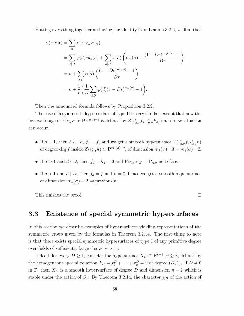
Putting everything together and using the identity from Lemma 3.2.6, we find that

χ(Fixσ) =∑α

χ(Fixα σ|X)

=∑d-D

ϕ(d)md(σ) +∑d|D

ϕ(d)

(md(σ) +

(1−Dr)md(σ) − 1

Dr

)

= n+∑d|D

ϕ(d)

((1−Dr)md(σ) − 1

Dr

)

= n+1

r

(1

D

∑d|D

ϕ(d)(1−Dr)md(σ) − 1

).

Then the announced formula follows by Proposition 3.2.2.

The case of a symmetric hypersurface of type II is very similar, except that now the

inverse image of Fixα σ in Pmd(α)−1 is defined by Z(ι∗α,σfd, ι∗α,σhd) and a new situation

can occur.

• If d = 1, then hd = h, fd = f , and we get a smooth hypersurface Z(ι∗α,σf, ι∗α,σh)

of degree deg f inside Z(ι∗α,σh) ' Pm1(σ)−2, of dimension m1(σ)−3 = m′1(σ)−2.

• If d > 1 and d - D, then fd = hd = 0 and Fixα σ|X = Pα,σ as before.

• If d > 1 and d | D, then fd = f and h = 0, hence we get a smooth hypersurface

of dimension md(σ)− 2 as previously.

This finishes the proof.

3.3 Existence of special symmetric hypersurfaces

In this section we describe examples of hypersurfaces yielding representations of the

symmetric group given by the formulas in Theorem 3.2.14. The first thing to note

is that there exists special symmetric hypersurfaces of type I of any primitive degree

over fields of sufficiently large characteristic.

Indeed, for every D ≥ 1, consider the hypersurface XD ⊂ Pn−1, n ≥ 3, defined by

the homogeneous special equation PD = xD1 + · · ·+ xDn = 0 of degree (D, 1). If D 6= 0

in F, then XD is a smooth hypersurface of degree D and dimension n − 2 which is

stable under the action of Sn. By Theorem 3.2.14, the character χD of the action of

68

Sn on Hn−2pr (X) is given by the class function

χD = (−1)n(

1 +1

D

∑d|D

ϕ(d)((1−D)md − 1

)).

For small values of n one can explicitly decompose it into irreducible characters of Sn.

Proposition 3.3.1. The character χpr of S3 acting on the primitive cohomology of a

S3-curve of type I and bidegree (D, 1) satisfies

6χD =

(D − 1)(D − 5) 1⊕ (D − 1)(D + 1) sg ⊕ 2(D − 1)(D − 2)V if (D, 6) = 1,

(D − 2)(D − 4) 1⊕ (D − 2)(D + 2) sg ⊕ 2(D − 1)(D − 2)V if (D, 6) = 2,

(D − 3)2 1⊕ (D2 + 3) sg ⊕ 2D(D − 3)V if (D, 6) = 3,

(D2 − 6D + 12) 1⊕D2 sg ⊕ 2D(D − 3)V if (D, 6) = 6,

where V denotes the irreducible representation of degree 2 of S3.

Proof. One only needs to compute the inner products of χpr with 1, sg and V .

In particular, χ1 = χ2 = 0, and

χ3 = 2 · sg,

χ4 = 2 · sg ⊕ 2 · V,

χ6 = 2 · 1⊕ 6 · sg ⊕ 6 · V,

χ7 = 2 · 1⊕ 8 · sg ⊕ 10 · V,

and these are the only cases where some irreducible representation of S3 occur with

multiplicity at most 2.

On the other hand, special symmetric hypersurfaces of type II need not exist in

all primitive degrees, as the representation theory of Sn imposes certain conditions on

the value of the parameters for which they can exist.

Proposition 3.3.2. For ` ≥ 1, let θ′` be the class function on Sn defined by

θ′` = `m′1 = `m1−1.

If there exist a special Sn-hypersurface of type II and bidegree (D, 1), then θ′D−1 is the

character of a characteristic 0 representation of Sn.

69

Proof. Suppose X = Z(f, h) is a bidegree (D, 1) special Sn-hypersurface of type II,

and let Y be a special Sn-hypersurface of type I of bidegree (D, 1), e.g. given by

PD = 0 as above. Then, by Theorem 3.2.14, in the character χ of the representation

of Sn on Hn−2pr (X)⊕Hn−3

pr (Y ), the terms corresponding to d > 1 cancel out to leave

χ =(−1)n

D

(((1−D)m1 − 1

)−((1−D)m1−1 − 1

))= (−1)n−m1(D − 1)m1−1.

Claim. For every permutation σ ∈ Sn, sg(σ) = (−1)n−m1(σ).

Indeed, write σ = σ1 · · ·σm as a product of disjoint cycles, of lengths λ1, . . . , λm.

Then

sg(σ) =m∏i=1

sg(σi) =m∏i=1

(−1)λi−1 = (−1)∑mi=1(λi−1) = (−1)n−m.

Hence, as the character of Hn−2pr (X)⊕Hn−3

pr (Y ) computed above is χ = sg⊗ θ′D−1,

we conclude that θ′D−1 = sg ⊗ χ is the character of a representation of Sn.

We can also consider the closely related class function θ` := `θ′` = `m1 on Sn.

Proposition 3.3.3. For ` ≥ 1, θ` = `m1 is the character of a representation of Sn.

Proof. Let R be any finite ring with ` elements, and consider T := Rn, the R-linear

standard permutation representation of Sn, as a set on which Sn acts. We can then

form the associated E-linear permutation representation E[T ], thought of as the set

of functions T → E. The value of the character of this representation at σ ∈ Sn

is χE[T ](σ) = |FixT (σ)|. Let λ(σ) = λ1, . . . , λm be the partition associated to σ.

Without loss of generality, we can assume that σ lies in the image of Sλ1 × · · · × Sλmin Sn under the standard embedding; then it is easy to check that

FixT (σ) = (r1, . . . , r1︸ ︷︷ ︸λ1

, . . . , rm, . . . , rm︸ ︷︷ ︸λm

) | r1, . . . , rm ∈ R.

Since the set of fixed points FixT (σ) is a free R-module of rank m1(σ), we conclude

that

χE[T ](σ) = |FixT (σ)| = |R|m1(σ) = `m1(σ) = θ`(σ).

Thus θ` is the character of the E-linear representation of Sn on E[T ].

As m1 ≥ 1 on Sn, certainly all the values of θ` = `m1 are divisible by `, i.e. the

values of θ′` are integers. To ask whether θ′` is a character or not is equivalent to ask

70

whether

(θ′`, φ) =1

`(θ`, φ) ∈ N, i.e. ` | (θ`, φ),

for all irreducible representations φ of Sn.

Proposition 3.3.4. If ` is prime, then θ′` = `m1−1 is the character of a representation

of Sn if and only if ` - n.

Proof. For (⇐), let R = Z/`Z and consider the function f : Rn → R defined by

f(r1, . . . , rn) =∑ri. If Sn acts on Rn via the standard permutation representation

and trivially on R, then the short exact sequence

0 −→ Ker f −→ Rn −→ R −→ 0

of R[Sn]-modules splits via the section r 7→ n−1(r, . . . , r) because n is invertible in R.

Hence Rn = R⊕Ker f as R-linear representations, which imply that E[Rn] is isomor-

phic to E[R]⊗ E[Ker f ], and since E[R] is an `-dimensional trivial representation, it

follows that the character of E[Ker f ] is θ`/` = θ′`.

Now for (⇒), suppose that θ′` is the character of a representation of Sn. In partic-

ular, the multiplicity (θ′`,1) = (θ`,1)/` of the trivial character in θ′` is a non-negative

integer.

Claim.

(θ`,1) =1

n!

∑σ∈Sn

`m1(σ) =

(n+ `− 1

n

).

Indeed, the left-hand side is the dimension of the space of invariants E[Rn]Sn =

E[Rn/Sn], so this multiplicity is the number of orbits for the action of Sn on Rn.

The orbits correspond to unordered lists r1, . . . , rn of elements of R, with repetition

allowed, and the number of these is the number of ways to put n identical balls (the

coefficients ri) into ` boxes (the elements of R), which is given by the right-hand side.

Hence, if θ′` is the character of a representation, then ` divides

(θ`,1) =

(n+ `− 1

n

)=

(n+ `− 1) · · · (n+ 1)

(`− 1)!.

Since ` is prime, it has to divide n+ i for some 1 ≤ i < `, hence cannot divide n.

Along with Proposition 3.3.2, this combinatorial fact yields the following.

Corollary 3.3.5. When ` is a prime, no special Sn-hypersurface of type II and bide-

gree (`+ 1, 1) can exist when ` | n.

71

Remark. The proof of Proposition 3.3.4 actually shows that even when ` is composite,

θ′` is a character of Sn when (n, `) = 1, because the only thing that was needed was

that n be invertible in Z/`Z. This suggests the following conjecture:

θ′` is a character of Sn ⇐⇒ (n, `) = 1.

In addition of being true when ` is prime, this conjecture was checked by explicitly

computing the decomposition into irreducibles of θ` for n ≤ 5, as well as machine

computations for n, ` ≤ 20. A proof in the general case probably requires explicit

formulas for other multiplicities (θ`, φ), φ 6= 1. If the conjecture is true, it means that

a special Sn-hypersurface of type II and bidegree (D, 1) can only exist when n and

D − 1 are coprime.

It is important to note that not all hypersurfaces in Pn−1 or in the diagonal

hyperplane H ' Pn−2 which are stable under the permutation action of Sn are special.

Nevertheless, Corollary 3.2.11 can still be used to compute the character χpr of Sn on

their primitive cohomology. Here is an interesting example.

Example 3.3.6. Consider the 1-parameter family of curves Wα:β ⊆ P3 defined by

4∑i=1

xi = α

( 4∑i=1

x4i

)+ β

( 4∑i=1

x2i

)2

= 0, (α : β) ∈ P1.

Computing the appropriate discriminant, they are seen to be smooth over any field

of characteristic different from 2 outside the exceptional values

(α : β) ∈ (0 : 1), (2 : −1), (4 : −1), (12 : −7).

Using Corollary 3.2.11, one finds that χpr is given by the following table.

σ 1 (12) (123) (12)(34) (1234)

χpr 6 −2 0 −2 2

It is thus readily seen that

χpr = 2 · (sg ⊗ Perm),

where Perm denotes the irreducible permutation representation of S4.

This family can be described in another way, taking advantage of the exceptional

72

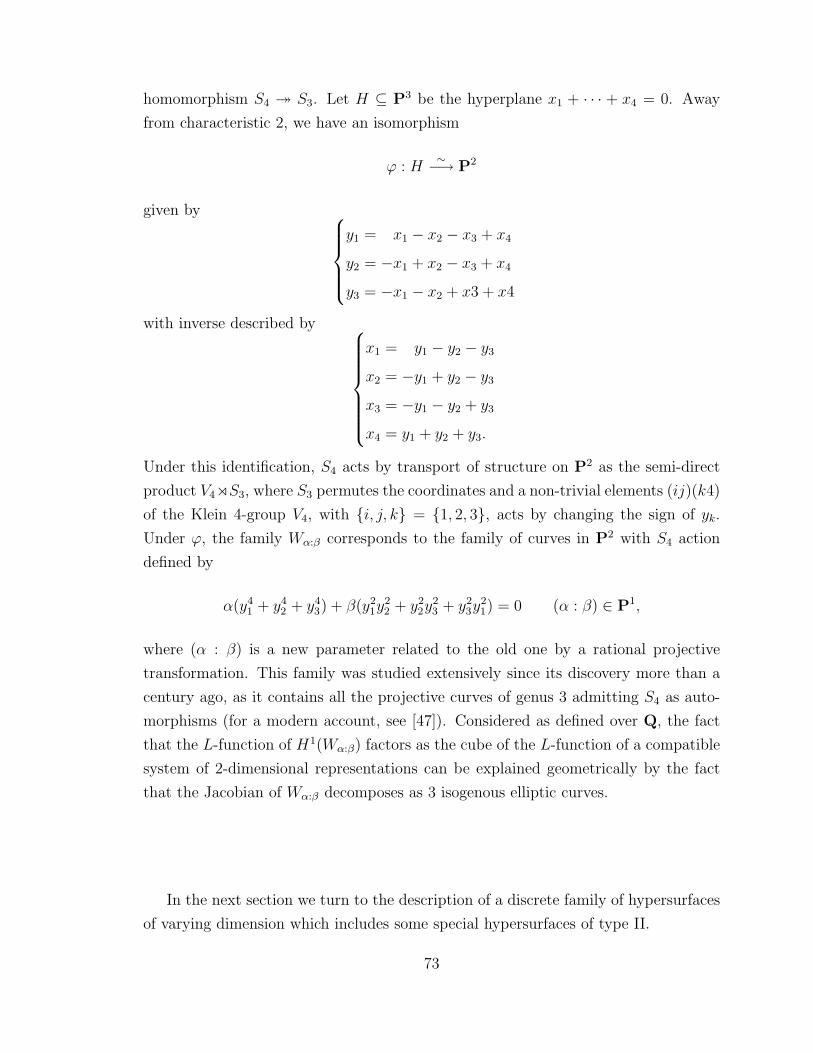
homomorphism S4 S3. Let H ⊆ P3 be the hyperplane x1 + · · · + x4 = 0. Away

from characteristic 2, we have an isomorphism

ϕ : H∼−→ P2

given by y1 = x1 − x2 − x3 + x4

y2 = −x1 + x2 − x3 + x4

y3 = −x1 − x2 + x3 + x4

with inverse described by

x1 = y1 − y2 − y3

x2 = −y1 + y2 − y3

x3 = −y1 − y2 + y3

x4 = y1 + y2 + y3.

Under this identification, S4 acts by transport of structure on P2 as the semi-direct

product V4oS3, where S3 permutes the coordinates and a non-trivial elements (ij)(k4)

of the Klein 4-group V4, with i, j, k = 1, 2, 3, acts by changing the sign of yk.

Under ϕ, the family Wα:β corresponds to the family of curves in P2 with S4 action

defined by

α(y41 + y4

2 + y43) + β(y2

1y22 + y2

2y23 + y2

3y21) = 0 (α : β) ∈ P1,

where (α : β) is a new parameter related to the old one by a rational projective

transformation. This family was studied extensively since its discovery more than a

century ago, as it contains all the projective curves of genus 3 admitting S4 as auto-

morphisms (for a modern account, see [47]). Considered as defined over Q, the fact

that the L-function of H1(Wα:β) factors as the cube of the L-function of a compatible

system of 2-dimensional representations can be explained geometrically by the fact

that the Jacobian of Wα:β decomposes as 3 isogenous elliptic curves.

In the next section we turn to the description of a discrete family of hypersurfaces

of varying dimension which includes some special hypersurfaces of type II.

73

3.4 The hypersurfaces Wm,n`

Throughout this section we fix two integers m,n ≥ 0 and F an algebraically closed

field in which (m+n)! 6= 0. Let Am+n denote the affine space Am×An over F, and by

convention, points in Am+n will be written as (x,y) with x ∈ Am, y ∈ An. Similarly,

Pm+n−1 will denote the projective space P(Am+n), with homogeneous coordinates

[x; y]. Thus, as before, m+ n refers to the number of variables.

Definition 3.4.1. For any integer ` ≥ 1, let Wm,n` denote the projective variety in

Pm+n−1 defined by the two homogeneous equations

m∑i=1

xi =n∑j=1

yj,m∑i=1

x`+1i =

n∑j=1

y`+1j .

To alleviate the notation, we will denote W 0,n` by W n

` .

These varieties will arise naturally in our study of distribution of certain exponen-

tial sums in the next chapter, generalizing the study of W n2 made by Livne [38] in

connection with cubic exponential sums.

Note that the varietiesWm,n` could be considered as schemes over Z. They admit an

action of the product Sm×Sn via its standard embedding in Sm+n which permutes the

homogeneous coordinates in Pm+n−1. In particular, W n` is an hypersurface admitting

an action of Sn defined by the power polynomials

p1 = p`+1 = 0,

hence will be a special Sn-hypersurface of type II and bidegree (` + 1, 1) when it is

smooth. And of course,

Wm,n` ' W n,m

`

under the automorphism of Pm+n−1 which interchanges the roles of x and y, so we

will often make the tacit assumption that n ≥ m.

Our first task is to decide when these varieties are smooth, and to describe their

singular locus when they are not.

Lemma 3.4.2. Suppose that ` 6= −1 in F. The singular locus of Wm,n` can be described

as the set of points [x,y] ∈ Pm+n−1 with all homogeneous coordinates xi, yj ∈ µ`(F)

74

and satisfyingm∑i=1

xi =n∑j=1

yj.

Proof. The Jacobian matrix(1 · · · 1 −1 · · · −1

(`+ 1)x`1 · · · (`+ 1)x`m −(`+ 1)y`1 · · · −(`+ 1)y`n

)

has rank 1 if and only if

(`+ 1)x`i = (`+ 1)y`j = λ, i = 1, . . . ,m, j = 1, . . . , n,

for some constant λ ∈ F. Since `+ 1 is invertible in F and at least one homogeneous

coordinate can be taken to be 1, these conditions reduce to

x`i = y`j = 1,

i.e. all the homogeneous coordinates xi, yj can be taken to be `th roots of unity in F.

Since a`+1 = a for a ∈ µ`(F), the two conditions that such a point has to satisfy to

belong to Wm,n` degenerate to the single equation

∑i xi =

∑j yj.

We can get a slightly more explicit description of the singular locus as follows.

Proposition 3.4.3. Let ζ be a primitive `th root of unity in F, and mζ(t) its minimal

polynomial over the prime field F0. If ` 6= 1 in F, the singular locus of Wm,n` is the

set of points of the form

σ · [ ζ0︸︷︷︸m0

: ζ1︸︷︷︸m1

: · · · : ζ`︸︷︷︸m`

: ζ0︸︷︷︸n0

: ζ1︸︷︷︸ : · · · : ζ`︸︷︷︸n`

]

where σ ∈ Sm × Sn and∑

k(nk −mk)tk is divisible by mζ(t) in F0[t].

Proof. Let [x; y] be a point whose homogeneous coordinates are `th roots of unity,

and for every 0 ≤ k ≤ `, let

mk := |i | xi = ζk| and nk := |j | yj = ζk|.

75

According to Lemma 3.4.2, the condition that [x; y] is a singular point becomes∑k

mkζk =

∑k

nkζk,

i.e. the polynomial∑

k(nk −mk)tk ∈ F0[t] vanishes at t = ζ.

We will now restrict ourselves to situations for which we have an explicit knowledge

of mζ(t). Recall that if F has characteristic 0 and ` is prime, then

mζ(t) = Φ`(t) =t` − 1

t− 1= 1 + t+ · · ·+ t`−1.

In positive characteristic p, for ` a prime different from p, the degree of mζ(t) is seen

to be the smallest integer r for which ` | pr − 1, i.e. the order of p in (Z/`Z)×. It

follows that the degree of mζ(t) is ` − 1 precisely when the prime p is inert in the

cyclotomic extension Q(ζ`).

By a small abuse of terminology, we will decreet that 0 is inert in Q(ζ`), so that

we have

mζ(t) = 1 + t+ · · ·+ t`−1 ⇐⇒ char F is inert in Q(ζ`).

Under this condition, we can give an explicit description of the singularities of Wm,n` .

Proposition 3.4.4. Let ` be a prime such that char F is inert in Q(ζ`) and ` 6= −1

in F. If ` - n −m, then Wm,n` is a smooth hypersurface of dimension m + n − 3. If

n−m = a`,

SingWm,n` = Sm × Sn · [x; ζ0︸︷︷︸

a

: ζ1︸︷︷︸a

: · · · : ζ`−1︸︷︷︸a

: x] | x ∈ µ`(F)m,

and these singularities are all ordinary double points. More precisely, the tangent cone

at a singular point t ∈ SingWm,n` is a smooth quadric Qt defined over F0(t) ⊆ F0(ζ).

When its dimension is even, it has signed determinant

∆ =

1 if ` = 2,

(−1)a/2 if ` > 2.

Proof. When char F is inert in Q(ζ`), Proposition 3.4.3 tells us that there exists an

76

integer a such that`−1∑k=0

(nk −mk)tk = aΦ`(t) in F0[t],

i.e. the differences mk − nk are all congruent modulo the characteristic of F. But the

integers nk−mk lie in the bounded interval [−n,m] of length m+n. If F has positive

characteristic, then by our hypothesis we have char F > m+ n so that the differences

mk − nk actually have to be equal in Z. In all cases, we conclude that there exists an

integer a ∈ Z such that nk = mk + a for 0 ≤ k < `.

Summing over k, we find that this implies n = m + a`, so clearly Wm,n` can have

no singularities when ` - n−m. On the other, when ` | n−m, by writing n = m+ a`

we obtain the announced description for the singular locus.

Let us now consider a singular point [x; y] with xi = ζri and yj = ζsj . Setting

zi = xi + ζri and wj = yj + ζsj in the equations for Wm,n` , we get

∑i

zi −∑j

wj = 0,`+1∑u=0

(`+ 1

u

)(∑i

zui ζri(`+1−u) −

∑j

wuj ζsj(`+1−u)

)= 0.

Without loss of generality, let us assume that r0 = s0 = 0. Then, setting w0 = 0, we

get affine equations for the tangent cone,∑i

zi =∑j

′wj,

∑i

z2i ζ−ri =

∑j

′w2j ζ−sj

where∑′ means that we omit the index 1. From the first equation, we can isolate

w1 =∑i

′zi −

∑j

′wj

and substitute in the second one to get∑′(1 + ζ−ri)z2

i + 2∑′

zizi′ +∑′

(1− ζ−sj)w2j + 2

∑′wjwj′ − 2

∑′ziwj = 0.

In other terms, the tangent cone is a quadric Q(t) with defining matrix(E −D −E−E E +D1

),

where the E’s denote matrices having all entries 1, D is the diagonal matrix with

77

the ζri ’s on its diagonal (2 ≤ i ≤ m), and D1 the diagonal matrix with the ζsj ’s

(2 ≤ j ≤ n). Up to a reordering of the variables, D1 can be written as(D

δ

), δ = diag(Ia, ζIa, . . . , ζ

`−1Ia).

Using standard manipulations, the matrix for Q(t),E −D −E −E−E E +D E

−E E E + δ

can be transformed into D − I D

D 0

E + δ

.

Now write D as diag(I, D′) where no entry in D′ is 1. Then the first block in the

above quadric is equivalent to the square matrix of size 2(m− 1)× 2(m− 1)

diag(2I, −2I, D′ − I, −(D′ − I)) ∼ diag(I,−I),

which has determinant (−1)m−1 6= 0, and signed determinant ∆ = 1.

Lemma 3.4.5. If δ = diag(d1, . . . , dn) is a diagonal matrix with non-zero entries,

then

det(E + δ) = det δ

(1 +

n∑i=1

1

di

).

Proof. By adding a line of 1’s and using elementary row operations, we get

det(E + δ) = det

(E + δ 0

E 1

)= det

(δ −EE 1

).

In the permutation expansion for the determinant of this last matrix, the only con-

tributing terms are those associated to the identity and the transpositions (i n+ 1),

i = 1, . . . , n, yielding

det(E + δ) =n∏j=1

dj +n∑i=1

∏j 6=i

dj = det δ

(1 +

n∑i=1

1

di

),

78

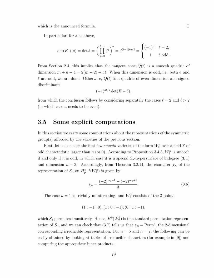
which is the announced formula.

In particular, for δ as above,

det(E + δ) = det δ =

( `−1∏j=0

ζj)a

= ζ(`−1)`a/2 =

(−1)a ` = 2,

1 ` odd.

From Section 2.4, this implies that the tangent cone Q(t) is a smooth quadric of

dimension m + n− 4 = 2(m− 2) + a`. When this dimension is odd, i.e. both a and

` are odd, we are done. Otherwise, Q(t) is a quadric of even dimension and signed

discriminant

(−1)a`/2 det(E + δ),

from which the conclusion follows by considering separately the cases ` = 2 and ` > 2

(in which case a needs to be even).

3.5 Some explicit computations

In this section we carry some computations about the representations of the symmetric

group(s) afforded by the varieties of the previous section.

First, let us consider the first few smooth varieties of the form W n2 over a field F of

odd characteristic larger than n (or 0). According to Proposition 3.4.5, W n2 is smooth

if and only if n is odd, in which case it is a special Sn-hypersurface of bidegree (3, 1)

and dimension n − 3. Accordingly, from Theorem 3.2.14, the character χn of the

representation of Sn on Hn−3pr (W n

2 ) is given by

χn =(−2)m1−1 − (−2)m3+1

3. (3.6)

The case n = 1 is trivially uninteresting, and W 32 consists of the 3 points

(1 : −1 : 0), (1 : 0 : −1); (0 : 1 : −1),

which S3 permutes transitively. Hence, H0(W 32 ) is the standard permutation represen-

tation of S3, and we can check that (3.7) tells us that χ3 = Perm, the 2-dimensional

corresponding irreducible representation. For n = 5 and n = 7, the following can be

easily obtained by looking at tables of irreducible characters (for example in [9]) and

computing the appropriate inner products.

79

Proposition 3.5.1. We have the following decompositions into irreducibles:

χ5 = sg ⊕ ψ,

χ7 = 2 · sg ⊕ (sg ⊗ Perm)⊕ θ,

where ψ is an irreducible character of degree 5 of S5, and θ an irreducible character

of degree 14 of S7.

Considering W 52 and W 7

2 as defined over Q, the compatible systems of Galois

representations of GalQ afforded by corresponding multiplicities and whose existence

is guaranteed by Theorem 3.1.4 will be explicitly computed in Chapter 5. Of particular

interest is the 2-dimensional compatible system

Msg(H4pr(W

72 )).

Let us write down further facts about W 72 for future reference in Section 5.7.

Proposition 3.5.2. The variety W 72 has good reduction outside 3, 5, 7 and primitive

Hodge numbers

h0,4 = h4,0 = 0, h1,3 = h3,1 = 1, h2,2 = 20.

Proof. From Proposition 3.4.5, we know that W 72 has good reduction for all primes

p > 7. We need to show that it has good reduction at p = 2, i.e. that the variety

W 72 over F2 is smooth. Lemma 3.4.2 still applies to show that the singularities in

characteristic 2 are all the points with projective coordinates which are square roots

of 1 lying in W 72 . But the only square root of 1 over F2 is 1, and the point

(1 : 1 : 1 : 1 : 1 : 1 : 1)

does not belong to W 72 . The Hodge numbers are obtained by expanding the generating

series of Proposition 2.3.4 up to order 4.

Note that the same argument used in the proof actually shows that for n odd, the

smooth hypersurface W n2 has good reduction at 2.

80

Chapter 4

Distribution of exponential sums

This chapter is concerned with how exponential sums of the form

∑x∈Fq

exp

(2πi

ptrFq/Fp(f(x))

)

are distributed, on average, as q → ∞. By this, we mean that for every fixed prime

power q = pr, we consider the set of all such exponential sums corresponding to

polynomials f ∈ Fq[x] of a fixed degree (in fact, we will also specify a set of weights

corresponding to the powers of x that are allowed to appear in f). We are interested

in the behavior of this set as q → ∞, where it will always be understood that the

characteristic p goes to infinity along with q. The motivation for this problem starts

with the Sato-Tate conjecture [62]: if E is an elliptic curve over Q without complex

multiplication, the angles

θp(E) := cos−1

(ap(E)

2√p

)are equidistributed as p→∞ with respect to the measure sin2 θdθ. As the coefficient

ap(E) = |E(Fp)| − p− 1 appearing above can be interpreted as the trace of Frobp on

the Tate module of E, this is really a conjecture about the distribution of the traces of

Frobenius elements as p varies; a general framework for problems this type have been

considered (see e.g. [55]). Birch [4] proved that the Sato-Tate conjecture holds on

average, the average being taken over the set of Weierstrass equations y2 = x3 +αx+β

for elliptic curves over Fp. In the same paper, he suggested that the same should be

81

true if the coefficients ap(Eα,β) appearing above are replaced by the exponential sums

Bp(α, β) =∑x∈Fp

exp

(2πi

p(αx3 + βx)

), α, β ∈ Fp, α 6= 0.

This conjecture was later proved by Livne [38] by relating the nth moment of

the average of these exponential sums to the number of points on the variety W n2

from Chapter 3 (in our notation). Asymptotics for the moments were obtained by

analyzing the etale cohomology of these varieties, thus proving Birch’s conjecture that

the exponential sums Bp(α, β), when normalized to lie in [−1, 1] by dividing by 2√p,

are equidistributed on average with respect to the Sato-Tate measure when p→∞.

It should be noted that etale cohomology enters in two distinct ways in the picture.

The first one is providing the bound 2√p for the values of the exponential sums

Bp(α, β) under consideration. This follows from a very general machinery which

interprets exponential sums as the traces of Frobenius on etale cohomology with values

in a certain sheaf, from which estimates can be derived by purity [14, 32, 37]. The

second way is by relating the moments of the average of these exponential sums to

the number of points on varieties of varying dimension, which can then be estimated

or computed using etale cohomology as well.

In this chapter we generalize Livne’s treatment of the cubic exponential sums

mentioned above by allowing more general sets of weights for the polynomial f . We

first give in Section 4.1 a short discussion trying to explain the theoretical importance

of these exponential sums by interpreting them as Fourier transforms for the function

counting the number of solutions of a system of equations over Fq, as is well-known.

In Section 4.2 we give a brief review of the relevant notions from measure theory to

justify why equidistribution problems can be translated into the study of the limit

behavior of the relevant moments.

In Section 4.3, we define a very general class of exponential sums and, generalizing

Livne, prove a key result (Theorem 4.3.2) relating the moments of their average with

the number of points on certain varieties. A significant difference with [38] is that the

cubic exponential sums considered there are real-valued, so that a 1-parameter family

of moments is enough to study their distribution. In our case, the exponential sums

are in general complex-valued, hence a 2-parameter family of moments is needed. This

is why the relevant varieties come with a “bipartite” action of Sm×Sn (instead of Sn

only in [38]).

In Section 4.4 we finally specialize to very specific sets of weights for which the

82

understanding of the cohomology of the relevant varieties is within our reach. Ac-

cordingly, after discussing a few easy cases, we concentrate mainly on the case of

exponential sums of weights 1, ` + 1, where ` is prime (note that the case ` = 2

was the one studied by Livne). In this case, the relevant varieties are the varieties

Wm,n` introduced in Section 3.4. Referring to Schoen’s results (Section 2.5) about the

cohomology of hypersurfaces with ordinary double points, we see that the moments

are essentially related to the subprimitive cohomology of Wm,n` (or rather, its dual, the

“supprimitive cohomology”). The main result is Theorem 4.4.7, which states precisely

this relationship, generalizing the main result of [38].

It should be pointed out however that, except in some special cases, this does not

prove that the exponential sums are equidistributed on average, but merely provides

formulae for the moments of the limit distribution, if it exists. To prove equidistri-

bution, one would need to know that these limits are actually the moments of some

measure. This fact, although probably true (see [29]), is not proven here.

4.1 Exponential sums as Fourier transforms

Exponential sums, under various guises, are ubiquitous in number theory. For an

overview of their many uses, see e.g. [34]. Here is one way of justifying their theoretical

importance, following Katz [28], by interpreting them as the Fourier transforms of the

number of solutions of equations over finite fields.

Let f ∈ Z[x] be a polynomial. Over any finite field Fq, one may consider the

equation f(x) = 0, or more generally the equation f(x) = α, for α ∈ Fq. The number

of solutions off all these equations, for fixed q, is encoded by the function

Nf,q : Fq −→ N, α 7→ |x ∈ Fq | f(x) = α|.

We lose no information if we consider Nf,q as a complex-valued function on the

additive group Fq, and as such we can consider its Fourier decomposition

Nf,q =∑ψ∈Fq

Nf,q(ψ)ψ, with Nf,q(ψ) =∑α∈Fq

Nf,q(α)ψ(α) =∑x∈Fq

ψ(f(x)).

Now the choice of a non-trivial additive character ψq on Fq identifies Fq with Fq via

a 7→ ψa,q, where ψa,q(x) = ψq(ax). Under this identification, the Fourier coefficients

83

of Nf,q are given by

Nf,q(a) =∑x∈Fq

ψq(af(x)).

More generally, if we start with a finite collection f = (f1, . . . , fm) ∈ Z[x]m of

polynomials, we can just as well consider the counting function for the corresponding

system of equations

Nf ,q : Fmq −→ N, (α1, . . . , αm) 7→ |x ∈ Fq | fi(x) = αi, i = 1, . . . ,m|,

whose Fourier coefficients are given by

Nf ,q(a) =∑x∈Fq

ψq(a1f1(x) + · · · amfm(x)),

and these are precisely the kind of exponential sums we want to consider here. In

particular, obtaining asymptotics for these exponential sums yields information about

the limit behavior of Nf ,q as q → ∞, i.e. about how the number of solutions of the

original system of equations behaves over larger and larger finite fields.

4.2 Equidistribution

This section summarizes the basic notions of measure theory which lie at the core of

this chapter. Let X be a compact metric space, and denote by B(X) the set of all

finite signed Borel measures on X. We endow B(X) with the topology of “setwise”

convergence, i.e. we say that νn → ν if νn(A)→ ν(A) for all Borel sets A.

Proposition 4.2.1 (Riesz representation theorem). The pairing

ν(f) :=

∫X

fdν

identifies B(X) with the continuous dual of the space C(X) of real-valued continuous

functions on X (equipped with the norm of uniform convergence).

Since characteristic functions of Borel sets can be uniformly approximated by

continuous functions, we see that

νn → ν ⇐⇒ νn(f)→ ν(f) for all f ∈ C(X),

84

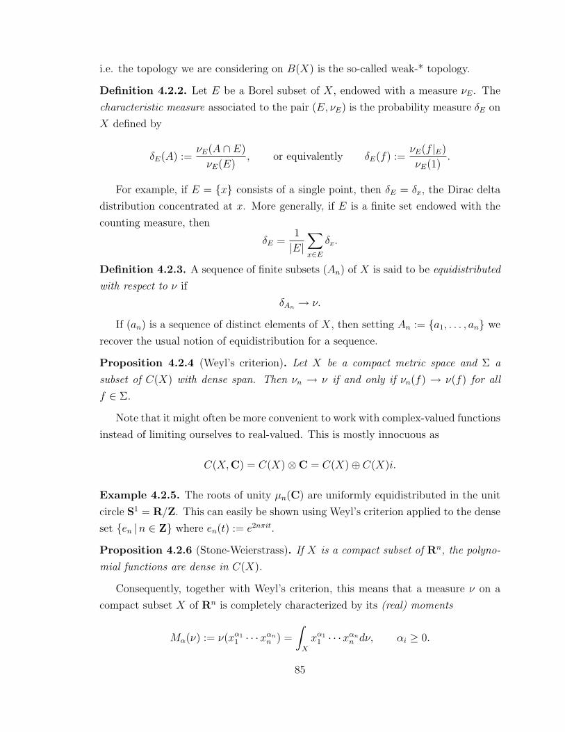
i.e. the topology we are considering on B(X) is the so-called weak-* topology.

Definition 4.2.2. Let E be a Borel subset of X, endowed with a measure νE. The

characteristic measure associated to the pair (E, νE) is the probability measure δE on

X defined by

δE(A) :=νE(A ∩ E)

νE(E), or equivalently δE(f) :=

νE(f |E)

νE(1).

For example, if E = x consists of a single point, then δE = δx, the Dirac delta

distribution concentrated at x. More generally, if E is a finite set endowed with the

counting measure, then

δE =1

|E|∑x∈E

δx.

Definition 4.2.3. A sequence of finite subsets (An) of X is said to be equidistributed

with respect to ν if

δAn → ν.

If (an) is a sequence of distinct elements of X, then setting An := a1, . . . , an we

recover the usual notion of equidistribution for a sequence.

Proposition 4.2.4 (Weyl’s criterion). Let X be a compact metric space and Σ a

subset of C(X) with dense span. Then νn → ν if and only if νn(f) → ν(f) for all

f ∈ Σ.

Note that it might often be more convenient to work with complex-valued functions

instead of limiting ourselves to real-valued. This is mostly innocuous as

C(X,C) = C(X)⊗C = C(X)⊕ C(X)i.

Example 4.2.5. The roots of unity µn(C) are uniformly equidistributed in the unit

circle S1 = R/Z. This can easily be shown using Weyl’s criterion applied to the dense

set en |n ∈ Z where en(t) := e2nπit.

Proposition 4.2.6 (Stone-Weierstrass). If X is a compact subset of Rn, the polyno-

mial functions are dense in C(X).

Consequently, together with Weyl’s criterion, this means that a measure ν on a

compact subset X of Rn is completely characterized by its (real) moments

Mα(ν) := ν(xα11 · · ·xαnn ) =

∫X

xα11 · · ·xαnn dν, αi ≥ 0.

85

If X is a compact subset of Cn ' R2n with coordinates zj = xj + iyj, then since

C[x1, y1, . . . , xn, yn] = C[z1, z1, . . . , zn, zn],

we can use instead the (complex) moments

Mα,β(ν) := ν(zα11 zβ1

1 · · · zαnn zβnn ), αi, βi ≥ 0.

The problem of trying to reconstruct the measure ν from its moments Mα(ν), or

even deciding whether a sequence of numbers are the moments of some measure, has

a long and interesting history, see e.g. [58]. In the case where X = [0, 1], this is called

the Hausdorff moment problem. However, we shall not be too much concerned with

these matters here.

A classical example of an equidistribution result in number theory is Dirichlet’s

theorem on the distribution of primes in arithmetic progressions, which can be stated

as: for every fixed m ∈ N, the images of the set of primes

En := p - m, p ≤ n

are uniformly equidistributed in (Z/mZ)× as n→∞.

More generally, we have the following well-known result, strengthening the state-

ment of Proposition 1.4.3.

Proposition 4.2.7 (Chebotarev density theorem). Let K be a number field and L a

finite Galois extension of K. Then the sets

En := Frobp | p prime of K unramified in L,N(p) ≤ n

are uniformly equidistributed amongst the weighted conjugacy classes of Gal(L/K).

4.3 Exponential sums

For every finite field Fq with q = pr elements, consider ψq : (Fq,+) → C× a fixed

non-trivial additive character. To every nonempty finite subset κ ⊂ N of weights, and

86

vector a = (ak)k∈κ ∈ Fκq , with amaxκ 6= 0, we associate the exponential sum

Bκ(q, a) :=∑x∈Fq

ψq

(∑k∈κ

akxk

)∈ C. (4.1)

Following Birch [4] and Livne [38], we would like to understand how these complex

numbers are distributed, on average, when q →∞ (here it will always be understood

that p→∞ as q →∞).

A trivial case is when κ = 1 or κ = 0, 1; then it is easily seen that Bκ(q, a) = 0

for all a with a1 6= 0. This can be rephrased by saying that these exponential sums are

equidistributed with respect to the Dirac distribution δ0 concentrated at the origin.

In other cases, the Weil estimate coming from purity [14] yields the following.

Proposition 4.3.1. If maxκ > 0 and p > maxκ, then |Bκ(q, a)| ≤ (maxκ− 1)√q.

From now on, we will assume that maxκ > 1, i.e. we exclude the trivial cases

considered above. Then the normalized exponential sums

bκ(q, a) :=Bκ(q, a)

(maxκ− 1)√q

lie in the closed unit disk D = z ∈ C : |z| ≤ 1, and we would like to understand

their limit average distribution as q →∞ (if it exists). More precisely, let δκ(q) denote

the characteristic measure associated to the finite set

bκ(q, a) | a ∈ Fκ

q , amaxκ 6= 0.

From Section 4.2, we know that a measure on D is determined by its action on the

monomials zmzn, for m,n ≥ 0. If δκ(q) has a limit measure ν as q → ∞, then the

moments of δκ(q) converge to the moments of ν. As a consequence, we would like to

understand the asymptotic behavior of the quantities

Mm,nκ (q) := Mm,n(δκ(q)) =

1

q|κ|−1(q − 1)

∑a

′bκ(q, a)mbκ(q, a)

nas q →∞,

where∑′ means that the sum ranges over all vectors a = (ak)k∈κ ∈ Fκ

q with amaxκ 6= 0.

Letting N = m+ n, for ease of manipulation we will prefer to work instead with the

87

closely related quantities

V m,nκ (q) := (maxκ− 1)NqN/2Mm,n

κ (q)

=1

q|κ|−1(q − 1)

∑a

′Bκ(q, a)mBκ(q, a)

n (4.2)

Define Wm,nκ,aff to be the variety in Am+n = AN cut out by the |κ| homogeneous

equationsm∑i=1

xki =n∑j=1

ykj (k ∈ κ),

and let Wm,nκ the projective variety in PN−1 over which Wm,n

κ,aff is the affine cone. The

following proposition, generalizing [38, lemma 4.1] attributed to Birch, is key to our

analysis by relating the moments of exponential sums to the number of points on the

varieties Wm,nκ,aff .

Theorem 4.3.2. Let κ′ := κ \ maxκ. Then

V m,nκ (q) =

1

q − 1

(q |Wm,n

κ,aff(Fq)| − |Wm,nκ′,aff(Fq)|

).

In particular, this formula implies that V m,nκ (q), hence the limit distribution as

q → ∞ of the exponential sums (4.1), if it exists, does not depend on the choice of

the additive character ψq 6= 1.

Proof. By splitting the sum∑

a∈FκqBκ(q, a)mBκ(q, a)

ninto terms with amaxκ = 0 and

terms with amaxκ 6= 0, using the expression (4.2) for V m,nκ we obtain∑

a∈Fκq

Bκ(q, a)mBκ(q, a)n

=∑

a′∈Fκ′q

Bκ′(q, a′)mBκ′(q, a′)

n+ q|κ|−1(q − 1)V m,n

κ (q). (4.3)

Now, by using (4.1) and distributivity, we find

∑a∈Fκq

Bκ(q, a)mBκ(q, a)n

=∑a∈Fκq

( m∏i=1

Bκ(q, a)

)( n∏j=1

Bκ(q, a)

)

=∑a∈Fκq

( m∏i=1

∑xi∈Fq

∏k∈κ

ψq(akxki )

)( n∏j=1

∑yj∈Fq

∏k∈κ

ψq(−akykj )

)

=∑

x∈Fmq

∑y∈Fnq

∏k∈κ

∑ak∈Fq

ψq

(ak

( m∑i=1

xki −n∑j=1

ykj

)).

88

But by orthogonality of characters, we have

∑ak∈Fq

ψq

(ak

( m∑i=1

xki −n∑j=1

ykj

))=

q if (x,y) ∈ Wm,nk,aff ,

0 else,

from which is follows that

∏k∈κ

∑ak∈Fq

ψq

(ak

( m∑i=1

xki −n∑j=1

ykj

))=

q|κ| if (x,y) ∈ ∩k∈κWm,nk,aff = Wm,n

κ,aff ,

0 else.

Consequently, ∑a∈Fκq

Bκ(q, a)mBκ(q, a)n

= q|κ| |Wm,nκ,aff(Fq)|,

and by the exact same argument applied to κ′ we get∑a′∈Fκ′q

Bκ′(q, a′)mBκ′(q, a′)

n= q|κ|−1 |Wm,n

κ′,aff(Fq)|.

Substituting these two last expressions in (4.3) and isolating V m,nκ (q) concludes the

proof.

Corollary 4.3.3. If |κ| ≥ 2 and 0 ∈ κ, then

Mm,nκ (q) =

0 if m 6= n,

Mm,nκ\0 if m = n.

Proof. First, note that if κ is a set of weights such that 0 ∈ κ, then one of the defining

equations of Wm,nκ,aff is m = n, so that

Wm,nκ,aff =

∅ if m 6= n,

Wm,nκ\0,aff if m = n.

Hence, if 0 ∈ κ and |κ| ≥ 2, then 0 ∈ κ′ as well, and the above remark applies to

both κ and κ′ to give

Wm,nκ,aff = Wm,n

κ′,aff = ∅ when m = n,

Wm,nκ,aff = Wm,n

κ\0,aff , Wm,nκ′,aff = Wm,n

κ′\0,aff when m 6= n.

89

The conclusion follows by Theorem 4.3.2 and formula (4.2).

Consequently, without real loss of generality we can restrict our attention to the

cases where 0 /∈ κ.

Corollary 4.3.4. When 0 /∈ κ, κ 6= ∅,

V m,nκ (q) = 1 + q |Wm,n

κ (Fq)| − |Wm,nκ′ (Fq)|.

Proof. In this situation, since Wm,nκ,aff is the affine cone over Wm,n

κ , we have

|Wm,nκ,aff(Fq)| = 1 + (q − 1)|Wm,n

κ (Fq)|,

and similarly for κ′. It then follows from Theorem 4.3.2 that

V m,nκ =

1

q − 1

(q + q(q − 1)|Wm,n

κ (Fq)| − 1− (q − 1)|Wm,nκ′ (Fq)|

),

which simplifies to the announced expression.

It follows that asking for an asymptotic as q →∞ for V m,nκ is the same as asking

for asymptotics for the number of points on the projective varieties Wm,nκ , which can

in principle be read from their etale cohomology thanks to the trace formula.

4.4 Equidistribution results

In this section, we look at the cohomology of the varieties Wm,nκ in increasing order

of complexity for κ to derive the corresponding statements for the moments of the

exponential sums bκ(q, a), using the machinery developed in the previous section.

Case κ = k, k > 1. Suppose that p = char Fq > k, so that Wm,nκ is a smooth

hypersurface of degree k and dimension N − 2 over Fq. Since as Galois modules we

have (Corollary 2.3.3)

H•(Wm,nκ ) ' H•(PN−2)⊕HN−2

pr (Wm,nκ ),

the trace formula yields

|Wm,nκ (Fq)| =

qN−1 − 1

q − 1+ (−1)N tr(Frobq | HN−2

pr (Wm,nκ )).

90

From Corollary 4.3.4 and the fact that Wm,n∅ = PN−1, we get

V m,nκ (q) = 1 + q

(qN−1 − 1

q − 1+ (−1)N tr(Frobq | HN−2

pr (Wm,nκ ))

)−(qN − 1

q − 1

)= (−1)N q tr(Frobq | HN−2

pr (Wm,nκ )).

From (4.2), it follows that

Mm,nκ (q) =

(−1)N

(k − 1)NqN/2−1tr(Frobq | HN−2

pr (Wm,nκ )). (4.4)

We see that, in this case, a precise asymptotic for Mm,nκ (q) as q → ∞ depends

crucially on the Galois representation afforded by the primitive cohomology of Wm,nκ .

We can obtain a crude estimate for the moments by using purity, which guarantees

that

| tr(Frobq | HN−2pr (Wm,n

κ ))| ≤ q(N−2)/2 dimHN−2pr (Wm,n

κ )

= qN/2−1 (k − 1)N + (−1)N(k − 1)

k.

by the formula for the dimension of the primitive cohomology of a smooth hypersurface

(Corollary 2.3.5). Using this upper bound in (4.4), we find that

|Mm,nκ (q)| ≤ 1

k

(1 +

(−1)N

(k − 1)N−1

).

In particular, the only conclusion that we may draw from purity is that if limit

Mm,nκ of the moments Mm,n

κ (q) as q →∞ exists, it satisfies

|Mm,nκ | ≤ 1

k

(1 +

(−1)N

(k − 1)N−1

).

One needs more information about the Galois representation on the primitive

cohomology, e.g. by evaluating the Gauss sums of Proposition 2.3.7 , to give a more

precise estimate.

Special case κ = 2. In this particular case, we can say more since Wm,nκ is a

smooth quadric of dimension N−2 provided p > 2, hence the discussion of Section 2.4

applies to give a complete description of the Galois representation on the primitive

cohomology.

91

Proposition 4.4.1. For κ = 2, the normalized exponential sums bκ(q, a), a 6= 0,

are equidistributed on average with respect to δ1,−1 when q →∞ along q ≡ 1 mod 4,

and with respect to δi,−i when q →∞ along q ≡ −1 mod 4.

Proof. When N = m + n is odd, the quadric Wm,nκ has no primitive cohomology, so

that (4.4) gives

Mm,nκ (q) = 0 (N odd).

On the other hand, when N = n + m is even, by Proposition 2.4.3, Frobq acts

on the 1-dimensional primitive cohomology by multiplication by qN/2−1 εq(∆) with

∆ = (−1)N/2(−1)n, so that

V m,nκ = q · qN/2−1(−1)(N

2+n) q−1

2 ,

hence from (4.4) we conclude that

Mm,nκ (q) = (−1)(N

2+n) q−1

2 (N even).

On the other hand, we can easily check that

Mm,n(δ1,−1) =1m+n + (−1)m+n

2=

1 + (−1)N

2,

Mm,n(δi,−i) =im(−i)n + (−i)min

2=iN(−1)n(1 + (−1)N)

2.

Thus Mm,nκ (q) = Mm,n(δ1,−1) when q ≡ 1 mod 4, while Mm,n

κ (q) = Mm,n(δi,−i)

when q ≡ −1 mod 4, and the conclusion follows.

This result exhibits what seems to be a fundamental feature of equidistribution

results for exponential sums: in general there might not exist a limit distribution as

q → ∞, but rather we expect different limit distributions along certain families of

values of q, controlling for example the presence of certain roots of unity in Fq.

Note that in this case we knew more a priori : when q ≡ 1 mod 4, since −1 is a

square in Fq,

bκ(q, a) =∑x∈Fq

ψq(−ax2) = bκ(q, a),

so that bκ(q, a) is actually a real number lying in the interval [−1, 1]. On the other

92

hand, when q ≡ −1 mod 4, we have instead

bκ(q, a) + bκ(q, a) =∑x∈Fq

ψq(−ax2) +∑x∈Fq

ψq(ax2) = 2

∑x∈Fq

ψq(ax) = 0,

so bκ(q, a) now lies in the imaginary interval [−i, i]. In both cases, Proposition 4.4.1

says that the normalized exponential sums accumulate towards the endpoints of the

interval on average as q →∞.

From Corollary 4.3.3 we deduce at once another equidistribution result.

Corollary 4.4.2. For κ = 0, 2, the normalized exponential sums bκ(q, a) are equidis-

tributed on average along the boundary of D, i.e. with respect to δS1, as q →∞.

Proof. From Corollary 4.3.3 and Proposition 4.4.1, we find that

Mm,nκ (q) =

0 when m 6= n,

1 when m = n..

These coincide with the moments of δS1 as

Mm,n(δS1) =

∫zmzndδS1 =

1

2π

∫ 2π

0

ei(m−n)θdθ =

0 when m 6= n

1 when m = n,

and the conclusion follows.

Case κ = 1, `+ 1. This is our main case of interest and the varieties Wm,nκ are

none other than the hypersurfaces Wm,n` from section 3.4. Following the geometrical

analysis carried out there, we restrict ourselves to the case where ` is prime.

Proposition 4.4.3. Let ` be a prime, κ = 1, ` + 1 and q = pr where p is a prime

which is inert in Q(ζ`). For ` - n−m,

Mm,nκ (q) = O

(1√q

).

In particular, for ` - n−m, Mm,nκ (q)→ 0 as q →∞ along inert primes.

Proof. Under these conditions, by Proposition 3.4.4, Wm,nκ is a smooth hypersurface

over Fp of degree ` + 1 and dimension N − 3, provided p > max(N, `). From Corol-

lary 2.3.3,

H•(Wm,nκ ) ' H•(PN−3)⊕HN−3

pr (Wm,nκ ),

93

from which it follows that

|Wm,nκ (Fq)| =

qN−2 − 1

q − 1+ (−1)N−3 tr(Frobq | HN−3

pr (Wm,nκ )). (4.5)

Moreover, since κ′ = 1, Wm,nκ′ ' PN−2, so that Corollary 4.3.4 yields

V m,nκ (q) = 1 + q

(qN−2 − 1

q − 1+ (−1)N−3 tr FrobqH

N−3pr (Wm,n

κ )

)− qN−1 − 1

q − 1

= (−1)N−3q tr FrobqHN−3pr (Wm,n

κ ).

(4.6)

By purity, this implies that

|V m,nκ (q)| ≤ q · q(N−3)/2 dimHN−3

pr (Wm,nκ ) = q(N−1)/2 dimHN−2

pr (Wm,nκ ).

Consequently, from (4.2) we obtain

|Mm,nκ (q)| ≤ 1

q

(1

`NdimHN−2

pr (Wm,nκ )

),

and the result follows.

This seems to suggest an `-fold rotational symmetry for the putative limit distri-

bution of the normalized exponential sums bκ along inert primes. For, suppose that

ν is a measure on the unit disk D which can be written in polar coordinates as

ν = f(r)g(θ)rdrdθ.

The corresponding moments are

Mm,n(ν) =

∫ 2π

0

∫ 1

0

rmeimθrneinθf(r)g(θ)rdrdθ

=

∫ 1

0

rm+n+1f(r)dr

∫ 2π

0

ei(m−n)θg(θ)dθ

= 2πMN+1(f) an−m(g),

where ak(g) is the kth Fourier coefficient of g. In particular, if all the moments of f

on [0, 1] are non-zero, then

Mm,n(ν) = 0 =⇒ an−m(g) = 0.

94

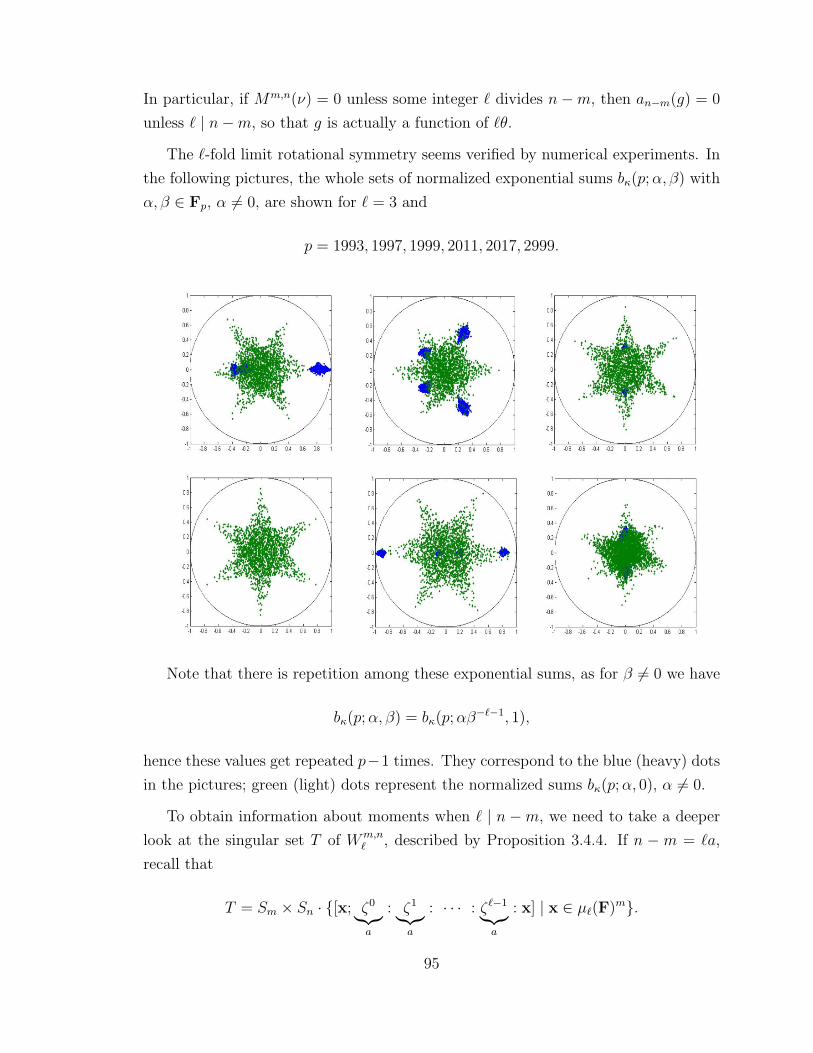
In particular, if Mm,n(ν) = 0 unless some integer ` divides n−m, then an−m(g) = 0

unless ` | n−m, so that g is actually a function of `θ.

The `-fold limit rotational symmetry seems verified by numerical experiments. In

the following pictures, the whole sets of normalized exponential sums bκ(p;α, β) with

α, β ∈ Fp, α 6= 0, are shown for ` = 3 and

p = 1993, 1997, 1999, 2011, 2017, 2999.

Note that there is repetition among these exponential sums, as for β 6= 0 we have

bκ(p;α, β) = bκ(p;αβ−`−1, 1),

hence these values get repeated p−1 times. They correspond to the blue (heavy) dots

in the pictures; green (light) dots represent the normalized sums bκ(p;α, 0), α 6= 0.

To obtain information about moments when ` | n −m, we need to take a deeper

look at the singular set T of Wm,n` , described by Proposition 3.4.4. If n − m = `a,

recall that

T = Sm × Sn · [x; ζ0︸︷︷︸a

: ζ1︸︷︷︸a

: · · · : ζ`−1︸︷︷︸a

: x] | x ∈ µ`(F)m.

95

If x ∈ µ`(Fq)m, let λi be the number of times that ζi appears as in x, 0 ≤ i < `.

We obtain this way a composition of m in at most ` parts, i.e. an ordered `-tuple

λ = (λ0, λ1, · · · , λ`−1) of non-negative integers adding up to m. Let us write λ |=` m

to signify that λ is such a composition of m in at most ` parts. These compositions

parametrize the orbits of Sm × Sn on T , and by taking scaling into account we find

that

|T (Fq)| =1

`

∑λ|=`

(m

λ

)(m+ a`

λ+ a

).

For ease of notation, let us now denote Wm,n` by W , and let W be its blow-up

along the singular set T . We can relate the number of points on W to that of W ,

generalizing [38, lemma 4.3].

Lemma 4.4.4. With ∆ as in Proposition 3.4.5 if n − m = `a is even, and the

convention that εq(∆) = 0 if n−m is odd, we have

|W (Fq)| = |W (Fq)| − q |T (Fq)|(qN−4 − 1

q − 1+ qN/2−3 εq(∆)

).

Proof. Since W \ T is isomorphic to W \ T over Fq, we have

|W (Fq)| = |W (Fq)|+ |T (Fq)| − |T (Fq)|. (4.7)

At the level of cohomology (cf. the discussion at the end of Section 2.5), we have

H•(T ) =⊕t∈T

H•(Qt) = H0(T )⊗H•(Q),

where Q is any fiber since they all carry the same Galois action by Propositions 2.4.3

and 3.4.5. It follows that

|T (Fq)| = |T (Fq)| |Q(Fq)| = |T (Fq)|(qN−3 − 1

q − 1+ qN/2−2 ε∆(q)

)with our convention that ε∆(q) = 0 if N is odd (that is, when Q, a smooth quadric of

dimension N − 4, has no primitive cohomology). Using this formula in (4.7) finishes

the proof.

96

Using this lemma, the formula of Corollary 4.3.4 now reads

V m,nκ = 1 + q |W (Fq)| − q2 |T (Fq)|

(qN−4 − 1

q − 1+ qN/2−3 ε∆(q)

)− qN−1 − 1

q − 1. (4.8)

Let us treat separately the case where N is even and the case where it is odd, since

we know from Section 2.5 that the cohomology of W will behave differently. The easy

case is when W has no subprimitive cohomology, that is, when its dimension N − 3

is even (cf. Proposition 2.5.5).

Proposition 4.4.5. For κ = 1, `+ 1, ` prime, N = m+ n odd and ` | n−m,

Mm,nκ (q) = O

(1√q

)−→ 0

as q →∞ along inert primes.

Proof. By the results of section 2.5, as Galois modules, for i ≤ N − 3 we have

H i(W ) ∼=

0 i odd,

1 i = 0,(1⊕H0(T )

)⊗ χi/2cycl i even 6= 0, N − 3,(

1⊕H0(T ))⊗ χi/2cycl ⊕HN−3

pr (W ) i = N − 3.

Using Poincare duality for N − 3 < i ≤ 2(N − 3), the trace formula yields

|W (Fq)| = 1 +N−4∑j=1

(1 + |T (Fq)|)qj + tr(Frobq | HN−3pr (W )) + qN−3

=qN−2 − 1

q − 1+ q |T (Fq)|

qN−4 − 1

q − 1+ tr(Frobq | HN−3

pr (W )).

Substituting this expression in (4.8), in which εq(∆) = 0 since the exceptional fibers

have odd dimension, everything cancels out, leaving only

V m,nκ (q) = q tr(Frobq | HN−3

pr (W )).

Putting this in (4.2) gives

Mm,nκ (q) =

1

`NqN/2−1tr(Frobq | HN−3

pr (W )),

97

and the conclusion follows from purity.

The case when N is even is more interesting, because then the exceptional fibers,

of dimension N−4, have primitive cohomology, and thus the subprimitive cohomology

of W does not vanish.

Proposition 4.4.6. For κ = 1, `+ 1, ` prime, N = n+m even and ` | n−m,

Mm,nκ (q) =

εq(∆)

`NdimHN−4

sub (W ) +O

(1√q

)for q above an inert prime.

Proof. Mimicking the proof of Proposition 4.4.5, this time Section 2.5 tells us that

|W (q)| = qN−2 − 1

q − 1+ q |T (Fq)|

qN−4 − 1

q − 1+ tr FrobqM

•,

with M• = HN−4sub (W ) ⊕HN−3

pr (W ) ⊕HN−4sub (W )∨(1). Substituting into (4.8), a lot of

cancelation still occurs to leave only

V m,nκ (q) = q tr(Frobq |M•)− qN/2−1 |T (Fq)| εq(∆).

From (4.2) we then obtain

Mm,nκ (q) =

1

`NqN/2−1

((1 + q) tr(Frobq | HN−4

sub (W ))− tr(Frobq | HN−3pr (W ))

).

From purity, the dominant term is seen to be

1

`NqN/2−1q tr(Frobq | HN−4

sub (W )) =1

`NqN/2−2tr(Frobq | HN−4

sub (W )).

Now, from Proposition 2.5.5, the subprimitive cohomology of W is the image of the

hyperplane classes spanning the primitive cohomology of the exceptional fibers; it

follows that Frobq acts on it by multiplication by q(N−4)/2εq(∆), from which the con-

clusion follows.

We summarize Propositions 4.4.3, 4.4.5 and 4.4.6 in the following theorem.

Theorem 4.4.7. Suppose that ` is a prime and κ = 1, `+1. For q of characteristic

p which is split in Q(ζ`), the moments of the normalized exponential sums bκ(q) can

98

be written as

Mm,nκ (q) = Nm,n

κ +O

(1√q

),

with Nm,nκ (q) = 0 if ` - n−m or 2 - n−m, and

Nm,nκ (q) =

εq(∆)

`NdimHN−4

sub (Wm,n` ) if 2, ` | n−m.

Using Corollary 4.3.3 we deduce the following.

Corollary 4.4.8. For κ = 0, 1, `+ 1, where ` is prime, the normalized exponential

sums bκ(q) are equidistributed on average with respect to the Dirac delta measure δ0

as q →∞ along inert primes in Q(ζ`).

Proof. By Corollary 4.3.3 and Theorem 4.4.7, we have Mm,nκ = 0 for all m,n ≥ 0,

which are indeed the moments of δ0.

In [38], Livne managed to obtain an explicit formula the dimension of the sub-

primitive cohomology appearing in Theorem 4.4.7 in the special case ` = 2, m = 0,

by using the isomorphism of Proposition 2.5.5 to compute its decomposition into irre-

ducibles as a representation for Sn. Such a task can be attempted in our case to obtain

explicit values for the average moments in terms of Kostka numbers, at least for some

specific values of the parameters; however, this will have to be pursued elsewhere.

99

100

Chapter 5

Comparing Galois representations

This chapter is devoted to criteria allowing to decide algorithmically whether two

`-adic representations of the absolute Galois group GalK of a number field K are

equivalent or not.

Faltings [17] was the first to remark that this could in principle be achieved through

a finite computation when the representations are ramified at only a finite number

of places. This was shortly afterwards turned by Serre [57] into a usable tool, the

so-called “method of quartic fields” (see Section 5.2) which allowed one to prove that

certain elliptic curves over Q were isogenous (for example in [40]).

Another instance of the criterion, applicable to 2-dimensional 2-adic representa-

tions with even trace, was devised and used by Livne [39] to prove the modularity of

the variety W 102 from Chapter 3. This version was widely used, for example in [50],

and in the recent years to show modularity of certain K3 surfaces and rigid Calabi-

Yau varieties (see [25] for a survey), before the proof of the Serre conjectures were

announced.

In section 5.1, the current state of affairs for 2-dimensional representations of

GalQ arising in the cohomology of varieties is discussed. In a nutshell, the Serre

conjectures imply that all such representations (satisfying some obvious requirements)

are modular; but an ad hoc tool might sometimes still be useful to pinpoint the exact

modular form in the absence of precise information about the ramification. And of

course, general techniques applicable in principle to more general situations are still

desirable.

We then try to work out the details of the Faltings-Serre method in a general set-

ting since the literature is very scarce on this subject, the best source being the very

concise summary [57]. We thus define in Section 5.2 the basic object of the construc-

101

tion, the deviation group of two integer-valued λ-adic representations of a group G,

which is a finite quotient of G on which we can check by computing traces whether or

not the two representations are equivalent. In Section 5.3 a more concrete quotient of

this deviation group is described in the case where the two initial representations are

not isomorphic. Showing that such a quotient cannot exist is thus sufficient to prove

that the two representations under consideration are indeed isomorphic, and this was

the way that Serre’s quartic fields method was used, for instance in [40]. It is also

true that in certain situations, this quotient could be advantageously substituted for

the deviation group; see the remark there.

In Section 5.4, the Faltings-Serre-Livne criterion for equivalence of 2-adic, 2-

dimensional representations with even trace is presented together with its proof. This

is the basis for our generalization, Theorem 5.5.13 of Section 5.5, in which we remove

the hypothesis of evenness of traces at the price of increasing the list of groups that

can arise. The precise criterion for Galois representations is stated in Theorem 5.5.15.

In order to apply this generalized criterion to compute the modular form associated

to the 2-dimensional compatible system of Galois representations arising in the prim-

itive cohomology of W 72 in Section 5.7, we first state some facts in Section 5.6 which

allows one to list all the quadratic extensions of a number field which are unramified

outside a given finite set of primes.

5.1 Isogeny and modularity

Faltings made his observation about the possibility of detecting the equivalence of

`-adic representations by a finite computation in connection with his work on abelian

varieties [17] in which he proved the following pair of results. Recall that if A is an

abelian variety of dimension g, its `-adic Tate module

T`(A) := lim←−n

A[`n]

is a free Z`-module of rank 2g.

Theorem 5.1.1. If A is defined over a number field K, then V`(A) := T`(A)⊗Q` is

a semisimple representation for the absolute Galois group GalK of K.

Theorem 5.1.2. For A and A′ two abelian varieties defined over a number field K,

102

the natural map

HomK(A,A′)⊗ Z` −→ HomZ`(T`(A), T`(A′))GalK

is an isomorphism.

Recall from section 1.1 that we use the notation V ∼ W to mean that two repre-

sentations in characteristic 0 are equivalent, i.e. that they have isomorphic semisim-

plifications.

Corollary 5.1.3. A and A′ are K-isogenous ⇐⇒ V`(A) ∼ V`(A′).

In particular, an algorithm to decide the equivalence of Galois representations

yields an algorithm to solve the isogeny problem (see for example [1]). In the special

case of elliptic curves over Q, the situation is considerably easier now that modularity

is known.

Theorem 5.1.4 (Modularity theorem). Let ρ be the compatible system of represen-

tations associated to an elliptic curve E over Q of conductor NE. Then there exists

a newform f ∈ S2(NE, 1) such that ρ ' ρf .

In particular, it implies that the isogeny problem for elliptic curves over Q is very

easy.

Corollary 5.1.5. Two elliptic curves E1 and E2 over Q are Q-isogenous if and only

if they have the same conductor NE1 = NE2 = N and |E1(Fp)| = |E2(Fp)| for all

primes p - N such that

p ≤ N

6

∏p|N

(1 +

1

p

).

Proof. Let ρi be the compatible system of 2-dimensional Galois representations asso-

ciated to Ei, and fi the corresponding modular form, for i = 1, 2. Then

E1 ∼ E2 ⇐⇒ ρ1 ∼ ρ2 ⇐⇒ f1 = f2.

By [44, th. 1], a cusp form f of weight 2 and level N is determined by its first

N

6

∏p|N

(1 +

1

p

)

103

Fourier coefficients an(f); for eigenforms, we can restrict our attention to Fourier

coefficients ap(f) where p is prime.

In our situation, if p | N , from multiplicity 1 it is automatic that ap(f1) = ap(f2)

since f1 and f2 are newforms of the same level N . For p - N , since

ap(fi) = tr ρi(Frobp) = 1− |Ei(Fp)|+ p,

the result follows.

More generally, the Serre conjectures (when they are completely proven) will imply

modularity for all reasonable 2-dimensional systems coming from the cohomology of

algebraic varieties. Recall that to a residual representation ρ : GalQ → GL2(F`), Serre

associates a triple of invariants: a weight k(ρ), a level N(ρ) and a character ε(ρ).

Conjecture 5.1.6 (Serre [54]). If ρ is odd and absolutely irreducible, then there exists

a newform f ∈ Sk(ρ)(N(ρ), ε(ρ)) such that ρ ∼ ρf .

As of 2008, a significant part of the conjecture is considered to be proved and a

full proof is expected soon.

Theorem 5.1.7 (Khare-Wintenberger [31]). The Serre conjecture is true when N(ρ)

is odd.

Corollary 5.1.8. Let ρ be a compatible system of 2-dimensional odd irreducible rep-

resentations of Hodge-Tate weights (a, b) arising in the cohomology of an algebraic

variety X defined over Q. Then, assuming the full Serre conjectures (or uncondi-

tionally if ρ is unramified at 2), there exists a newform f ∈ Sb−a(N, ε) such that

ρ ' χacycl ⊗ ρf , where ε = χ−2acycl ⊗ det ρ and

N |∏

p∈Ram ρ

Np,

with

Np =

28 if p = 2 /∈ Ram(det ρ),

211 if p = 2 ∈ Ram(det ρ),

35 if p = 3,

p2 if p > 5.

Here is an outline of the proof (for more details, see [54] or [30]).

104

Proof. Consider ρ′ := χ−acycl ⊗ ρ, which has Hodge-Tate weights (0, b − a). Setting

ε := det ρ′, we then have ε(ρ′`) = ε for all primes `, and k(ρ′`) = b − a for infinitely

many `. Also, for infinitely many primes `, one can show that the level N(ρ′`) has

to divide the bound on the conductor given above [54]. By the pigeonhole principle,

it follows that there exists a divisor N of that bound such that N(ρ′`) = N for an

infinite number of primes `.

Hence we conclude that the triple of Serre invariants associated to ρ′` is (b−a, ε,N)

for an infinite number of values of `. By the Serre conjectures, for each of these there

exists a newform f` ∈ Sb−a(N, ε) associated to ρ′`. Since there exists only a finite

number of such newforms, one finds a single f ∈ Sb−a(N, ε) such that for infinitely

many `, one has ρ′` ∼ ρf . But this means that for an infinite number of primes ` we

have

tr ρ′ ≡ tr ρf mod `,

which is only possible if tr ρ′ = tr ρf , i.e. ρ′ ' ρf .

Example 5.1.9. Let ρ be the 2-dimensional compatible system of representations of

GalQ afforded by Msg(H4pr(W

72 )), whose existence is guaranteed by Theorem 1.2.2 and

Proposition 3.5.1. In Section 5.7, we will see that ρ has Hodge-Tate weights (1, 3) and

that det ρ = χ4cycl ⊗ ε35, where ε35 is the quadratic character of conductor 35. Hence

5, 7 ⊆ Ram ρ ⊆ 3, 5, 7,

since W 72 has good reduction outside 3, 5, 7. It follows (unconditionally) from Corol-

lary 5.1.8 that

ρ ' χcycl ⊗ ρf ,

where f is a newform of weight 3, character ε35 and level dividing 35 52 72 = 297675.

However, numerical evidence suggests that the level of f is actually 35, as will be

proven in Section 5.7.

Keeping with the notations of Corollary 5.1.8, if we assume that the traces of

ρ(Frobp) for unramified primes p are computable, there exists in theory an algorithm

to determine f from ρ.

1. Find a finite set of primes S such that Ram ρ ⊆ S.

2. Make a list of all newforms f1, . . . .fr of the right weight, and level N dividing∏p∈S Np.

105

3. Compute successively all the traces tr ρ(Frobp) for p /∈ S; at each step, eliminate

fi if it does not have the right ap(fi).

4. Eventually only one newform is left (by 1.4.4); this is the f we are looking for.

In practice, the problem is that if (as is often the case) we do not know explicitly

the Artin conductor of ρ, we have to use the naive bound above, which is often

much too large to be practical. For example, if ρ comes from the cohomology of a

variety X, we can take for S the set of primes of bad reduction of X in step 1, but this

might be overkill. Thus we turn to a different kind of algorithm to compare Galois

representations, which can sometimes be used more efficiently to pinpoint the exact

modular form f .

5.2 Deviation groups

In this section, we introduce the basic construction involved in the Faltings-Serre

method, following loosely [57].

For the moment, let G be an arbitrary group, and Oλ the ring of integers in a local

number ring Eλ, with maximal ideal λ and residue field k. We consider two integer-

valued representations ρ1, ρ2 : G → GLn(Oλ) of G. The product homomorphism

ρ1 × ρ2 extends to an Oλ-algebra map

ρ : Oλ[G] −→ Mn(Oλ)⊕Mn(Oλ).

Let M be its image, and consider the composition

δ : G −→M× −→ (M/λM)×.

Definition 5.2.1. The image δ(G) of G in (M/λM)× will be called the deviation

group of the pair (ρ1, ρ2).

Proposition 5.2.2. δ(G) is a finite group. More precisely, |δ(G)| < |k|2n2.

Proof. M is a submodule of the free Oλ-module Mn(Oλ)⊕Mn(Oλ), hence M is itself

free, of rank

r ≤ rank(

Mn(Oλ)⊕Mn(Oλ))

= 2n2.

106

It follows that M/λM is a k-algebra of dimension r, hence

|δ(G)| ≤ |(M/λM)×| < |k|r ≤ |k|2n2

,

as claimed.

Remark. It might be tempting to think of δ(G) as a subgroup of GLn(k) × GLn(k),

but it is important to note that in general this is not the case. Indeed, consider the

short exact sequence associated to reduction modulo λ,

0 −→ Mn(λ) −→ Mn(Oλ) −→ Mn(k) −→ 0.

Writing R for the Oλ-algebra Mn(Oλ) ⊕ Mn(Oλ), it identifies Mn(k) ⊕ Mn(k) with

R/λR. Now call M the image of M in R/λR, so that

M = M/(M ∩ λR)

Since λM ⊆M ∩ λR, it follows that there is a short exact sequence

0 −→ (M ∩ λR)/λM −→M/λM −→M −→ 0.

Recall that the deviation group δ(G) is the image of G in (M/λM)×. Writing G

for the image of G in M× ⊆ (R/λR)× = GLn(k) × GLn(k), what we have is a short

exact sequence

1 −→ N(G) −→ δ(G) −→ G −→ 1, (5.1)

where the kernel N(G) is the image of ρ(G) ∩ (1 + λR) in (M/λM)×.

The following proposition shows that one can detect whether ρ1 and ρ2 are equiv-

alent by computing finitely many well-chosen traces, even though ρ1 and ρ2 typically

do not factor through any finite quotient of G.

Proposition 5.2.3. Let Σ be a subset of G surjecting onto δ(G). Then, as E-valued

representations,

ρ1 ∼ ρ2 ⇐⇒ tr ρ1|Σ = tr ρ2|Σ.

Proof. (⇒) is obvious. For (⇐), we prove the contrapositive. Suppose that ρ1 ρ2,

so that tr ρ1 6= tr ρ2, and let α be the greatest integer such that

tr ρ1 ≡ tr ρ2 mod λα.

107

Now choose an uniformizer π; the function π−α(tr ρ1 − tr ρ2) extends to an Oλ-linear

map

θ : M −→ Oλ, θ(M) * λ,

which descends to a nonzero k-linear map M/λM → k, hence to a function,

Θ : δ(G) −→ k,

which is nonzero because δ(G) spans M/λM . It implies that there exists an element

g ∈ Σ such that Θ(δ(g)) 6= 0, i.e.,

θ(g) = π−α(tr ρ1(g)− tr ρ2(g)) /∈ λ.

In particular, tr ρ1(g) 6= tr ρ2(g), so tr ρ1|Σ 6= tr ρ2|Σ.

Corollary 5.2.4. Let R be a class of representations of G defined over Oλ and Σ be

a subset of G surjecting onto all the deviation groups of pairs ρ1, ρ2 ∈ R. Then, given

two such representations ρ1 and ρ2,

ρ1 ∼ ρ2 ⇐⇒ tr ρ1|Σ = tr ρ2|Σ.

In particular, in light of Proposition 5.2.2, for R consisting of representations of

degree n, it is sufficient to ask that Σ surjects onto all quotients of G of size bounded

by |k|2n2. If G has only a finite number of such quotients, this yields in principle an

algorithm to decide the equivalence of n-dimensional λ-adic representations of G.

Application to Galois representations. We now specialize to the case where

G = GalK , the absolute Galois group of a number field K.

Lemma 5.2.5. Let ρ1 and ρ2 be two λ-adic representations of GalK. Then δ(GalK)

is unramified outside Ram ρ1 ∪ Ram ρ2.

Proof. For a prime p /∈ Ram ρ1 ∪ Ram ρ2, we have I(p) ⊂ Ker ρ1 ∩ Ker ρ2. It follows

that I(p) ⊂ Ker ρ, where ρ = ρ1 × ρ2. That is, the image ρ(GalK) is unramified at p.

Hence δ(GalK), being a finite quotient of ρ(GalK), is also unramified at p.

From this, we can deduce the following strengthening of Proposition 1.4.4.

Corollary 5.2.6. Given a finite set S of places of K and an integer n ≥ 1, there

exists a finite set of primes T disjoint from S such that if ρ1, ρ2 are any two λ-adic

108

representations of degree n of GalK, unramified outside S, then

ρ1 ∼ ρ2 ⇐⇒ tr ρ1|Σ = tr ρ2|Σ,

where Σ = Frobp | p ∈ T.

Proof. By the Hermite-Minkowski theorem, there are only a finite number of Galois

extensions L/K unramified outside S and of degree bounded by |k|2n2. One can take

for T a finite set of primes p for which the Frobenius substitutions Frobp exhaust all

conjugacy classes of Gal(L/K) for such extensions L/K.

Using effective Chebotarev density results, we can even give explicit bounds on

the required size of the set T appearing above. For K a number field and N a positive

integer, we define, following [1]:

∆∗(K,S,N) := |∆K/Q|N(N∏p∈S

p1−1/Np )N [K:Q],

where pp denotes the residual characteristic of the prime ideal p,

B(K,S,N) :=

∆∗(K,S,N)c if K 6= Q,

2∆∗(K,S,N)c if K = Q,

where c the absolute constant A1 of [35], as well as

B1(K,S,N) := 70(log ∆∗(K,S,N))2,

B2(K,S,N) := (4 log ∆∗(K,S,N) + 5N [K : Q]/2 + 5)2,

B′(K,S,N) := minB1(K,S,N), B2(K,S,N).

Theorem 5.2.7 (Effective Chebotarev). Let K be a number field, S a finite set of

places of K and L a finite Galois extension of K, of degree at most N , unramified

outside S. Then every conjugacy class of Gal(L/K) can be realized as Frobp with

NK/Q p ≤ B(K,S,N).

Under the generalized Riemann hypothesis, the same conclusion holds with B(K,S,N)

replaced by B′(K,S,N).

109

Corollary 5.2.8. Two `-adic n-dimensional representations ρ1 and ρ2 of K, unram-

ified outside S, are equivalent if and only if

tr ρ1(Frobp) = tr ρ2(Frobp)

for all unramified primes p of K such that

NK/Q p ≤ B(K,S, `2n2 − 1)

Under the generalized Riemann hypothesis, the same conclusion holds with B′.

Example 5.2.9. For K = Q, ` = 2, n = 2, ρ1, ρ2 unramified outside S = 2, 3, 5, 7,and assuming the generalized Riemann hypothesis, one would need to check that

tr ρ1(Frobp) = tr ρ2(Frobp) for all primes p 6= 2, 3, 5, 7 such that

p ≤ bB1(Q, S, 255)c = 137, 528, 394.

In particular, this is what one would have to go through to prove that the 2-adic

2-dimensional Galois representation in the primitive cohomology of W 72 considered in

Example 5.1.9 is associated to a newform of level 35.

5.3 The method of quartic fields

In order to gain more insight into the deviation group δ(G) associated to a pair

ρ1, ρ2 : G→ GLn(Oλ) of semisimple integer-valued λ-adic representations, we can try

to give it a concrete realization.

Let us suppose that the residual representations ρ1, ρ2 are equal, but that the

representations ρ1⊗E and ρ2⊗E are not isomorphic, i.e. conjugated by an element of

GLn(E). Let β be the maximal integer such that ρ1 and ρ2 are conjugated modulo λβ.

On one hand, the fact that ρ1 = ρ2 implies that β ≥ 1. On the other hand, since

ρ1 6' ρ2, there exists a maximal integer α such that tr ρ1 6≡ trρ2 mod λα, as in the

proof of Proposition 5.2.3. Hence certainly ρ1 and ρ2 are not conjugated modulo λα+1,

hence β ≤ α. In particular, this shows that β is finite. Moreover, by replacing ρ2 by

a conjugate if necessary, we can assume that

ρ1 ≡ ρ2 mod λβ, ρ1 6≡ ρ2 mod λβ+1.

110

We can thus write ρ2 = (1 + πβθ)ρ1, where θ : G → Mn(Oλ) is a function whose

image is not contained in the maximal ideal λ.

Proposition 5.3.1. If ρ1 6' ρ2, the function ϕ : G→ Mn(k)oGLn(k) defined by

g 7→ (θ mod λ, ρ1 mod λ)

is a group homomorphism which factors through the deviation group δ(G).

Proof. For g, h ∈ G, using

ρ2(g) = (1 + πβθ(g))ρ1(g),

ρ2(h) = (1 + πβθ(h))ρ1(h),

we find that

ρ2(gh) = ρ1(g)ρ1(h) + πβθ(g)ρ1(g)ρ1(h)

+ πβρ1(g)θ(h)ρ1(h) + π2βθ(g)ρ1(g)θ(h)ρ1(h).

Comparing this expression with ρ2(gh) = (1 + πβθ(gh))ρ1(gh), we find that

θ(gh) = θ(g) + θ(h)ρ1(g) + πβθ(g)θ(h)ρ1(g),

where xy denotes the conjugation yxy−1. Since β ≥ 1, it follows that

θ(gh) ≡ θ(g) + θ(h)ρ1(g) mod λ,

hence that ϕ(gh) = ϕ(g)ϕ(h) with the group law coming from the action of GLn(k)

on Mn(k) by conjugation.

Now, to show that ϕ factors through δ(G), we need to show that Ker δ ⊆ Kerϕ.

Let g ∈ Ker δ, which means that (using the notations of Section 5.2) ρ(g) ∈ 1 + λM ,

i.e., there exists elements ah ∈ Oλ, with ah = 0 for almost all h ∈ G, such that

ρ(g) = 1 + π∑h

ahρ(h).

Since ρ = ρ1 × ρ2, this is really a pair of equations

ρi(g) = 1 + π∑h

ahρi(h), i = 1, 2.

111

For i = 1, we see that this implies that ρ1(g) ≡ 1 mod λ. Moreover, using the fact

that ρ2 = (1 + πβθ)ρ1, the equation for i = 2 can be rewritten as

ρ1(g) + πβθ(g)ρ1(g) = 1 + π∑h

ahρ1(h) + π∑h

ahπβθ(h)ρ1(h).

Substracting the first equation, we find that

θ(g)ρ1(g) = π∑h

ahθ(h)ρ1(h),

hence

θ(g) = π∑h

ahθ(h)ρ1(hg−1) ≡ 0 mod λ,

so that ϕ(g) = (0, 1), i.e. g ∈ Kerϕ.

It ϕ(G) denotes the image of G in the semi-direct product Mn(k) o GLn(k), it

follows that the residual surjection δ(G) G of (5.1) can be refined to

δ(G) ϕ(G) G.

Note also that from ρ2 = (1 + πβθ)ρ1, we have

det ρ2 = (1 + πβ tr θ +O(πβ2

)) det ρ1,

so that if in addition we require that det ρ1 = det ρ2, it follows that

tr θ ≡ 0 mod λβ.

In particular, the homomorphism ϕ then has values in

Mn(k)oGLn(k),

where Mn denotes the set of n× n matrices of trace 0.

However, in general, δ(G) ϕ(G) may or may not be an isomorphism. From the

112

proof of Proposition 5.3.1, we see that an element g ∈ G lies in Ker δ if and only

ρ1(g) = 1 + π∑h

ahρ1(h), (5.2)

θ(g) = π∑h

ahθ(h)ρ1(h)ρ1(g)−1 (5.3)

for some ah ∈ Oλ, h ∈ G.

Proposition 5.3.2. For G = Z, ρ1 = 1 and ρ2 : G → GLn(Oλ) any non-trivial

semisimple representation such that ρ2 ≡ 1 mod λ, we have

δ(G) = ϕ(G) ' (k,+).

Proof. Since for any n ∈ G we have ρ2(n) = ρ2(1)n, we have

1 + πβθ(n) = (1 + πβθ(1))n =n∑j=0

(n

j

)πjβθ(1)j

by the binomial formula, so that

θ(n) =n∑j=1

(n

j

)π(j−1)βθ(1)j ≡ nθ(1) mod λ.

Consequently, if n ∈ Kerϕ, then π | n in Oλ, so that n = aπ for some a ∈ Oλ. But

then we may write

ρ1(n) = 1 + aρ1(1)− aρ1(0),

θ(n) = π(aθ(1)− aθ(0)

),

which show according to (5.2) that n ∈ Ker δ. Hence here Ker δ = Kerϕ, and the

conclusion follows.

Note that this proposition can be used to construct examples where δ(G) = ϕ(G)

and G is a profinite group. The representation ρ2 in the proposition, which is trivial

modulo λ, actually has values in 1+λMn(Oλ), which is a pro-`-group since it embeds

into the additive group λMn(Oλ) via the logarithm (` being the residual characteris-

tic). It follows that

ρ2 : Z −→ 1 + λMn(Oλ)

113

extends to Z`, and the proposition holds with G = Z`.

However, in certain situations, we can have Ker δ ( Kerϕ.

Remark. Serre, in [57], seems to imply that if ρ1, ρ2 : G → GL2(Z2) are two 2-adic

representations such that det ρ1 = det ρ2 and the residual representations ρ1 and ρ2

are equal and surjective, we have

δ(G) ' ϕ(G).

In a recent conversation with the author of this thesis, he said that maybe he did

not actually prove that the map δ(G) → ϕ(G) was surjective, but merely, in an

unpublished letter to Tate, that the β in the construction of ϕ was equal to the α in

the proof of Proposition 5.2.3, i.e. that ρ1 and ρ2 are conjugated modulo 2α if and

only if tr ρ1 ≡ tr ρ2 mod 2α. This would mean that the function

2−α(tr ρ1 − tr ρ2) mod 2,

considered in the proof of Proposition 5.2.3, descends to ϕ(G). Consequently, ϕ(G)

could be used in place of the deviation group in Corollary 5.2.4 as explained below,

making its application to decide whether two representations satisfying the hypotheses

of this remark are equivalent or not a lot easier.

Indeed, to make this even more explicit, note that note that as an S3-module,

under the action by conjugation of S3 ' GL2(F2),

M2(F2) ' F22 ⊕ V4,

with

F22 =

0, 1,

(1 1

1 0

),

(0 1

1 1

), V4 =

0,

(1 1

0 1

),

(0 1

1 0

),

(1 0

1 1

).

Likewise, the subgroup M2(F2) has the decomposition F2 ⊕ V4 with F2 = 0, 1.It follows that the only possibilities for ϕ(G) when det ρ1 = det ρ2 and ρ1 = ρ2 is

surjective are

±1 × S3, V4 o S3 ' S4, and (F2 ⊕ V4)o S3 ' ±1 × S4,

hence the name “quartic fields method”.

114

A last consequence worth remarking from the identity ρ2 = (1 + πβθ)ρ1 is that

tr ρ2 = tr ρ1 + πβ tr(θρ1),

and that tr(θρ1) ≡ tr(θρ1) mod λ. Thus,

π−β(tr ρ1 − tr ρ2) mod λ

descends to a function on ϕ(G). If ρ1 6∼ ρ2, and if the β from this section happens to

be equal to the α from the proof of Proposition 5.2.3, and Σ is a subset of G surjecting

onto ϕ(G), then we conclude that there exists g ∈ Σ such that

tr ρ1(g) 6= tr ρ2(g).

However, if β < α, then we are not guaranteed to find such a “certificate of non-

equivalence” in Σ if we merely require that Σ surjects onto ϕ(G).

5.4 The Faltings-Serre-Livne criterion

In this section we restrict our attention to 2-dimensional λ-adic representations

ρ1, ρ2 : G −→ GL2(Oλ)

where Oλ has residual characteristic 2. Moreover, we impose that

tr ρ1 ≡ tr ρ2 ≡ 0 mod λ and det ρ1 ≡ det ρ2 ≡ 1 mod λ. (5.4)

In this context, we present a proof of the Faltings-Serre-Livne criterion [39] to

decide whether ρ1 ∼ ρ2, in a form which will lend itself to generalization in the next

section. The following set will play a crucial role.

Definition 5.4.1. Define Ξ to be the set of elements g ∈ G for which the characteristic

polynomials of ρ1(g) and ρ2(g) coincide (or, equivalently, such that tr ρ1(gi) = tr ρ2(gi)

for i = 1, 2).

The strategy to decide whether ρ1 and ρ2 are equivalent, which will also be used in

the next section, can roughly be described as follows. Suppose we were to test every

element of G individually to see whether it belongs to Ξ or not. If we meet a single

115

element which is not in Ξ, meaning that Ξ 6= G, then we know that ρ1 ρ2. On the

other hand, if all the group elements that we encounter lie in Ξ, we might think that

there is “a good chance” that ρ1 and ρ2 are equivalent.

More precisely, call Σ the set of elements that we know are in Ξ. The bigger Σ is,

the stronger is the evidence that ρ1 and ρ2 might actually be equivalent, and we know

that to turn this evidence into a proof we just need to take Σ big enough so that it

surjects onto δ(G). The problem is that computing precisely δ(G) requires a lot more

information on ρ1 and ρ2 than we are able to get by computing a finite number of

traces. On the other hand, we might try to list all the possibilities a priori for δ(G),

and then just take Σ large enough to cover all such possibilities.

But then again, it is hard to say something precise on the structure of δ(G) (apart

from the bound on its size from Proposition 5.2.2). So we use a bootstrap strategy in

three steps.

• First, classify all possibilities for δ(G) if ρ1 and ρ2 were equivalent.

• Build sufficient evidence that ρ1 and ρ2 might be equivalent to force δ(G) to

actually belong to the list established in the previous step.

• Then take Σ large enough to cover all the possibilities for δ(G) in that list.

The “bootstrap” aspect of the strategy comes from the fact that what we want in

the end is a statement of the form if a large enough set Σ is known, then ρ1 and ρ2 are

equivalent (with a precise meaning of “large enough”), so the second and third step

of the strategy are actually achieved at the same time by having this large enough Σ.

So let us first see what δ(G) looks like when ρ1 and ρ2 are equivalent.

Proposition 5.4.2. If g ∈ Ξ, then δ(g)2 = 1 in δ(G).

Proof. For g ∈ Ξ, we write tr g for the common value of tr ρi(g), and similarly for

det g. Since the characteristic polynomials of ρ1(g) and ρ2(g) are equal, we have

ρ(g)2 = (tr g)ρ(g)− (det g)ρ(1).

Hence, by the hypothesis (5.4),

ρ(g)2 − ρ(1) = (tr g)ρ(g)− (det g + 1)ρ(1) ∈ λρ(g) + (2 + λ)ρ(1) ⊆ λM,

so that ρ(g)2 ≡ ρ(1) mod λM , i.e. δ(g)2 = δ(1) = 1 in δ(G).

116

Corollary 5.4.3. If ρ1 ∼ ρ2, then δ(G) is an abelian group of exponent 2.

Proof. If ρ1 ∼ ρ2, then Ξ = G, hence δ(G) = δ(Ξ) has exponent 2.

In general however, we cannot say much more than the following.

Proposition 5.4.4. The deviation group δ(G) is a 2-group.

More precisely, Proposition 5.2.2 implies that |δ(G)| = 2r with 0 ≤ r ≤ 7.

Proof. Recall from Remark 5.2 that δ(G) fits into a short exact sequence

1 −→ N(G) −→ δ(G) −→ G −→ 1

where N(G) is a finite quotient of ρ(G)∩(1+λR), where R = M2(Oλ)⊕M2(Oλ). Now

the multiplicative group 1 + λR embeds (via the logarithm) into the additive group

λR, hence is a pro-2-group. It follows (e.g. [3, Cor. 10.4]) that N(G) is a 2-group.

Moreover, by the condition 5.4, the characteristic polynomial of ρi, i = 1, 2, is

1− (tr ρi)t+ (det ρi)t2 ≡ 1 + t2 mod λ.

By Cayley-Hamilton, for every g ∈ G, one has

ρi(g)2 ≡ −1 ≡ 1 mod λ, i = 1, 2.

It follows that ρ(g)2 ≡ 1 mod λ, i.e. that G has exponent 2, hence in particular is

an abelian 2-group. So we conclude that δ(G), being an extension of G by N , is a

2-group.

The bootstrap process rests heavily on a technical group-theoretical lemma.

Definition 5.4.5. For H any group, we denote N2(H) = 〈h2 |h ∈ H 〉 the subgroup

generated by squares.

It is clear that N2(H) is a characteristic subgroup of H; hence we can consider

H2 := H/N2(H) the 2-quotient (for lack of a better term) of H.

Proposition 5.4.6. H2 is the greatest quotient of H of exponent 2. Moreover, if N

is a normal subgroup of H, then

(H/N)2 ' H/(N2(H) ·N).

In particular, (H/N)2 = H2 if and only if N ⊆ N2(H).

117

Proof. H/N is a quotient of H of exponent 2 if and only if N is a normal subgroup

which contains all the squares, that is, N ⊇ N2(H). The first part follows from the

fact that N2(H) is itself normal. For the second part, if N is any normal subgroup

of H, it is easily seen that N2(H/N) = (N2(H) · N)/N , from which the conclusion

follows.

We also use the notation H[2] for the set of elements of 2-torsion in H. Note that

H[2] need not be a subgroup of H when H is not abelian.

Lemma 5.4.7. Let H be a 2-group such that every element in H2 has a lift to an

element of H[2]. Then H has exponent 2, i.e. H = H2.

Proof. Consider the defining short exact sequence for H2,

1 −→ N2(H) −→ H −→ H2 −→ 1.

By contradiction: suppose that N2(H) 6= 1.

• Without loss of generality, we can assume that N2(H) is cyclic of order 2.

Indeed, let Ω be the set of subgroups of index 2 of N2(H). Writing the abelian-

ization of the 2-group N2(H) as

N2(H)ab =k⊕i=1

Z/2aiZ, k, ai ≥ 1,

we see that |Ω| = 2k − 1 is odd so that H acts on Ω by conjugation with at

least one fixed point N ∈ Ω. Replacing H by H/N (which doesn’t change its

2-quotient thanks to Proposition 5.4.6), we get the desired situation.

• Remark that N2(H) = 〈n〉 is then necessarily central: for h ∈ H, hnh−1 must

be an element of order 2 in N , hence hnh−1 = n.

• The elements of order 2 in H commute.

For two elements h, h′ of order 2, consider their product hh′. It is either of the

form h′′ or h′′n where h′′ has order 2. In both cases we see that (hh′)2 = 1.

• So we can find a section of H → H2 by picking generators of H2 and sending

them to some lifts of order 2 in H.

118

We conclude that H ' N×H2, which contradicts the definition of the 2-quotient.

With this tool we can derive a criterion for equivalence.

Theorem 5.4.8. Let ρ1, ρ2 : G → GL2(Oλ) be two representations satisfying condi-

tion (5.4), and

Ξ = g ∈ G | tr ρ1(g) = tr ρ2(g), det ρ1(g) = det ρ2(g).

Then ρ1 ∼ ρ2 if and only if Ξ surjects onto G2.

Proof. For (⇒) there is nothing to prove since Ξ = G. Now for (⇐), consider the

following diagram of quotients of G.

G // //

G2

δ(G) // // δ(G)2

Since Ξ surjects ontoG2 by hypothesis, it also surjects onto δ(G)2. But, by Proposition

5.4.2, the images of the elements of Ξ in δ(G) lie in δ(G)[2], hence we can apply the

lemma to δ(G) to conclude that δ(G) = δ(G)2. In particular, it follows that Ξ surjects

onto δ(G), which guarantees the equivalence of ρ1 and ρ2 by Proposition 5.2.3.

Actually, the version of the theorem proved in [39] is slightly stronger, stating that

ρ1 ∼ ρ2 if and only if the image of Ξ in G2, considered as an affine space over F2, is

not contained in any proper cubic hypersurface. However, this does not make a big

difference unless the set S of allowed ramification is large.

Application to Galois representations. This is the criterion essentially as is

stated in [39].

Theorem 5.4.9. Let K be a number field and Eλ a finite extension of Q2 with ring

of integers Oλ and maximal ideal λ. Let

ρ1, ρ2 : GalK −→ GL2(Eλ)

be two continuous representations unramified outside a finite set S of primes of K,

and such that

tr ρ1 ≡ tr ρ2 ≡ 0 mod λ and det ρ1 ≡ det ρ2 ≡ 1 mod λ.

119

Let K2,S be the compositum of all quadratic extensions of K unramified outside S and

suppose that there exists a set of primes T disjoint from S such that:

1. Frobp | p ∈ T surjects onto Gal(K2,S/K);

2. tr ρ1(Frobp) = tr ρ2(Frobp) and det ρ1(Frobp) = det ρ2(Frobp) for all p ∈ T .

Then ρ1 and ρ2 are equivalent.

Proof. Remark that since Gal(K/K) is compact, ρ1 and ρ2 preserve an Oλ-lattice in

E2λ, so that we may view them as taking values in GL2(Oλ). Then we only need to

apply the previous proposition to G = Gal(K/K)S = Gal(KS/K), where KS is the

maximal extension of K unramified outside S, since then G2 = Gal(K2,S/K).

To apply this criterion, one needs to describe explicitly the compositum K2,S of all

the quadratic extensions of K unramified outside S, together with its Galois group.

This will be addressed in general in section 5.6, but when K = Q the situation is

particularly simple.

• For p an odd prime, set dp =(−1p

)p so that Q2,p = Q(

√dp), and Frobt,

t /∈ S ∪ 2, goes to(dpt

)=(tp

)under

εp : Gal(Q/Q) −→ Gal(Q2,p/Q) ' ±1.

• Q2,2 = Q(i,√

2) = Q(ζ8), and Frobt, t /∈ S, goes to t mod 8 under

ε2 : Gal(Q/Q) −→ Gal(Q2,2/Q) ' (Z/8Z)×.

• For a general S, Q2,S =∏

p∈S Q2,p and

εS =∏p∈S

εp : Gal(Q/Q) −→ Gal(Q2,S/Q) '∏p∈S

Gal(Q2,p/Q).

So applying the criterion involves comparing the traces of ρ1 and ρ2 at 2|S|+1 primes

at most.

Example 5.4.10. This criterion was used in [38] to prove the modularity of the

compatible systems of representations of GalQ occurring in the middle-degree coho-

mology of W 102 . The trace of the representation could be shown to be even by using

the symmetries to show that the number of points over finite fields were always even.

120

5.5 Generalization

In this section, we restrict ourselves to the case Oλ = Z2 to keep the complexity under

control, but we only assume that

tr ρ1 ≡ tr ρ2 mod 2.

Note that in this context, it is automatic that det ρ1 ≡ det ρ2 ≡ 1 mod 2. We adapt

to this setting each result from the previous section. Recall that we use Cn to denote

the cyclic group of order n, and Sn for the symmetric group on n letters.

Proposition 5.5.1. In this setting, the residual group G is either isomorphic to 1,

C2, C2 × C2, C3, or S3.

Proof. In GL2(F2) ' S3, the elements of order 3 are those with trace 1, while the

elements with trace 0 have order 1 or 2. Thus the hypothesis on the traces of ρ1 and

ρ2 implies that for an element (x, y) in G ⊆ GL2(F2)×GL2(F2), one has

O(x) = 3 ⇐⇒ O(y) = 3.

If G contains no element (x, y) with O(x) = O(y) = 3, then

G ⊆ 1, (12), (13), (23) × 1, (12), (13), (23).

It is readily checked that G is then an abelian group of exponent 2 and order at

most 4.

On the other hand, suppose that G contains an element (x, y) where x and y have

order 3, so that it contains the cyclic subgroup H := 〈(x, y)〉. It is not possible that G

contains any other element of order 3, because then the order of G would be divisible

by 9, hence δ(G) would contain the whole 3-Sylow subgroup of S3 × S3,

1, (123), (132) × 1, (123), (132),

which is forbidden by the hypothesis on the traces.

If G 6= H, then G\H consists entirely of elements of the form (a, b) where a and b

both have order 2. If (a, b) and (a′, b′) are two distinct such elements, it is impossible

to have a = a′ or b = b′, because then the product (aa′, bb′) would have one trivial

121

component and the other of order 3. So, if (a, b) ∈ G \H, we see that

G = 1, (x, y), (x2, y2), (a, b), (ax, by), (ax2, by2) ' S3,

and this concludes the proof.

Corollary 5.5.2. The order of δ(G) is of the form 2a3b with b ≤ 1.

Again, together with Proposition 5.2.2, this implies that the order of the deviation

group is either 2a with 0 ≤ a ≤ 7, or 3 · 2a with 0 ≤ a ≤ 6.

Proof. This follows at once from the reduction modulo 2 short exact sequence

1 −→ N(G) −→ δ(G) −→ G −→ 1

and the previous proposition, because N(G) is a 2-group.

The following generalizes Proposition 5.4.8.

Proposition 5.5.3. Let ρ1, ρ2 : G→ GL2(Z2) be two representations such that tr ρ1 ≡tr ρ2 mod 2. Then ρ1 ∼ ρ2 if and only if Ξ surjects onto all quotients of G of the form

G/N2(W ), where W ranges over all the normal subgroups of G such that

G/W ' 1, C3 or S3.

Note that when W is normal, N2(W ) is automatically normal in G as well since

it is a characteristic subgroup of W .

Proof. Again (⇒) is clear because if ρ1 ∼ ρ2 then Ξ = G. Now for (⇐), if δ(G) is a

2-group, then, taking W = G, we conclude as in the proof of 5.4.8 that ρ1 ∼ ρ2. So

let us consider the case where the order of δ(G) is divisible by 3. Let W be the kernel

of the reduction map G→ G, so that G/W = G is isomorphic to C3 or S3, and let N

be the kernel of δ : G→ δ(G). The kernel N(G) in the short exact sequence

1 −→ N(G) −→ δ(G) −→ G −→ 1

is thus identified with W/N . Modding out by N2(N(G)), we obtain a new short exact

sequence

1 −→ N(G)2 −→ δ(G)/N2(N(G)) −→ G −→ 1.

122

Now N(G)2 is a quotient of exponent 2 of N(G) = W/N ; in particular, it is a quotient

of exponent 2 ofW , so N(G)2 is a quotient of the 2-quotient W2. We have the following

commutative diagram.

1 // W2//

G/N2(W ) //

G/W // 1

1 // N(G)2// δ(G)/N2(N(G)) // G // 1

By hypothesis, since G/W is isomorphic to C3 or S3, we know that Ξ surjects onto

G/N2(W ), so that it surjects onto δ(G)/N2(N(G)). It follows that every element of

N(G)2 has a lift in N(G)[2], so by Lemma 5.4.7, we conclude that N2(N(G)) = 1.

Hence Ξ actually surjects onto δ(G)/N2(N(G)) = δ(G), proving that ρ1 ∼ ρ2.

Corollary 5.5.4. Let K be a number field and ρ1, ρ2 : GalK → GL2(Q2) two con-

tinuous 2-adic Galois representations unramified outside a finite set of primes S and

such that tr ρ1 ≡ tr ρ2 mod 2 . If L/K is a Galois extension unramified outside S,

denote by L2,S the compositum of all quadratic extensions of L unramified at primes

above S (then L2,S is itself a Galois extension of K unramified outside S). Suppose

that there exists a set of primes T disjoint from S such that

1. Frobp | p ∈ T surjects onto Gal(L2,S/K) for all L/K with

Gal(L/K) ' 1, C3 or S3;

2. tr ρ1(Frobp) = tr ρ2(Frobp) and det ρ1(Frobp) = det ρ2(Frobp) for all t ∈ T .

Then ρ1 and ρ2 have isomorphic semisimplifications.

Example 5.5.5. This is essentially the approach used by Socrates and Whitehouse

[59] to prove that the Galois representation on the Tate module of a certain elliptic

curve E over Q(√

5) was associated to a Hilbert modular form f . More precisely, in

this example there was a priori only one possibility for W ⊆ GQ(√

5), the kernel of the

modulo 2 representations. Using the original Faltings-Serre-Livne criterion, one could

then prove that ρE and ρf were equivalent as representations of W , and then conclude

that are equivalent as GQ(√

5) as well using a Frobenius reciprocity argument.

Note that in practice, the first thing to do when trying to decide if two represen-

tations ρ1, ρ2 : G → GL2(Z2) are isomorphic is first to check whether the residual

123

representations ρ1 and ρ2 are conjugated in GL2(F2). If not, then ρ1 6' ρ2. If they

are conjugated, then without loss of generality when can assume that ρ1 = ρ2.

Remark. If two subgroups H1, H2 of GL2(F2) ' S3 have the same cardinality, then

not only are they abstractly isomorphic, but they are also conjugated. It follows that

if | Im ρ1| = | Im ρ2|, then without loss of generality, up to conjugation we may assume

that Im ρ1 = Im ρ2 since

1 −→ 1 + 2 M2(Z2) −→ GL2(Z2) −→ GL2(F2) −→ 1

splits. This does not, however, imply that the representations ρ1 and ρ2 are isomor-

phic.

It is possible to improve the straightforward generalization obtained in Proposi-

tion 5.5.3 by examining more carefully the possible structures of the deviation group.

Proposition 5.5.6. For g ∈ Ξ, the order of δ(g) in δ(G) is1 or 2 if tr g ≡ 0 mod 2,

3 if tr g ≡ 1 mod 2.

Proof. First, note that if δ(g) = 1, then g = 1 in G, so that the traces of ρ1(g) and

ρ2(g) are even. For g ∈ Ξ, we still have

ρ(g)2 = (tr g)g − det g ≡ (tr g)g + 1 mod 2M.

If tr g ≡ 0 mod 2, again δ(g)2 = 1 in M/2M hence in δ(G). If tr g ≡ 1 mod 2,

however, ρ(g)2 = ρ(g) + 1 in M/2M , so that

δ(g)3 = δ(g)(δ(g) + 1) = δ(g)2 + δ(g) = 1,

which concludes the proof.

Corollary 5.5.7. If ρ1 ∼ ρ2, every nontrivial element of δ(G) has order 2 or 3.

Hence, under the hypothesis that ρ1 ∼ ρ2, we know that δ(G) is a group of order

2a3b, with b = 0 or 1, in which every nontrivial element has order 2 or 3. Let us

classify all possibilities a priori for such a group.

Example 5.5.8. Of course, any finite group of exponent 2, i.e. C2r, is of this form.

124

Example 5.5.9. The symmetric group S3 is a group of order 6 in which every element

has order 2 or 3.

Example 5.5.10. Another important example is the alternating group A4: it is a

group of order 12 in which every nontrivial element has order 2 or 3. Remark that

A4 = V4 o C3, where C3 permutes cyclically the 3 nontrivial elements in the Klein

group

V4 = 1, (12)(34), (13)(24), (14)(23) ' C22.

More generally, if one considers the diagonal action of C3 on r copies of V4, the

semi-direct product V4r oC3 is a group of order 3 · 4r in which all nontrivial elements

have order 2 – those of the form (x, 1) – or 3 – those of the form (x, σ), σ 6= 1.

The following theorem states that these examples form a complete list of such

groups (up to isomorphism).

Theorem 5.5.11. The finite groups of order 2a3b, b = 0, 1, in which every nontrivial

element has order 2 or 3 are

C2r, r ≥ 0, V4

r o C3, r ≥ 0, and S3.

Proof. Let G be a group of order 2a3b, b = 0, 1, in which every nontrivial element has

order 2 or 3.

• First let us consider the easy case where b = 0: in this case G is a 2-group,

hence cannot contain any element of order 3. We conclude that G has exponent

2, so that G ' C2r for some r ≥ 0.

In the case where b = 1, we can distinguish two situations: the number of

2-Sylow subgroups of G is either 1 or 3.

• If there is a unique 2-Sylow subgroup P of G, then P is a normal subgroup and

we have a short exact sequence

1 −→ P −→ G −→ C3 −→ 1

which necessarily splits since G contains at least an element of order 3 which

we call σ. Moreover, P is a group of exponent 2 and we can consider it as a

finite-dimensional vector space over F2 on which C3 = 〈σ〉 acts linearly. Let

v ∈ P be a nonzero element. Then the element x := (v, σ) ∈ G = P oC3 has to

125

have order 3 by our assumption on the orders of elements of G; this is equivalent

to saying that

v + σ(v) + σ2(v) = 0.

If follows that the σ-invariant subspace generated by v is

0, v, σ(v), σ2(v),

which is isomorphic to V4 with the standard σ-action. By induction on the

dimension of P , it follows that P ' V r4 as a F2[σ]-module, hence

G = P o 〈σ〉 ' V4r o C3.

• The last case to consider is the case where the number of 2-Sylow subgroups in

G is 3. The action of G by conjugation on these 3 subgroups P1, P2, P3 yields a

homomorphism

G −→ S3

whose image is either C3 or S3 (because its kernel is a 2-group). But the former

is impossible, because then the kernel would be a normal 2-Sylow subgroup;

hence the latter holds and we have a short exact sequence

1 −→ N −→ G −→ S3 −→ 1.

Again we can check that this short exact sequence splits (using the fact that

the set of elements in G acting on the 2-Sylow subgroups as (ij) is Pk \ N for

i, j, k = 1, 2, 3), hence we may view G as N o S3 where N is a vector space

over F2 on which S3 acts.

Let τ be an element of order 2 in S3 ⊆ G and consider elements of the form

(v, τ) in G with v ∈ N . These need to have order 2, which means that

v + τ(v) = 0, or τ(v) = v for all v ∈ N.

Since S3 is generated by its elements of order 2, it follows that it acts trivially

on N , so that G = N × S3. Then, in order for G to contain no element of order

6, we need to have N = 1, i.e. G = S3.

This concludes the proof.

126

This group-theoretic fact, together with Corollary 5.5.7, Corollary 5.5.2 and the

remark directly following it, implies the following.

Corollary 5.5.12. If ρ1, ρ2 : G→ GL2(O) are two equivalent 2-adic representations

such that tr ρ1 ≡ tr ρ2 mod 2, then their deviation group is isomorphic to

Cr2 , 0 ≤ r ≤ 7, V r

4 o C3, 0 ≤ r ≤ 3, or S3.

We can now complete the “bootstrap” argument. Recall that the generalized

quaternion group Qn is defined by the presentation

Qn := 〈a, b | a2 = bn, b2n = 1, bab = a〉.

It has order 2n and fits into a non-split short exact sequence

1 −→ 〈τ〉 −→ Qn −→ Dn −→ 1,

where τ = a2 = bn is the unique element of order 2 in Qn.

Theorem 5.5.13. Let ρ1, ρ2 : G→ GL2(Z2) be two representations satisfying

tr ρ1 ≡ tr ρ2 mod 2.

Then ρ1 ∼ ρ2 if and only if

1. Ξ surjects onto all quotients of G of the form C2r, V4

r o C3, or S3;

2. The image of Ξ in every quotient of G of the form C6 or Q6 contains an element

of order 6;

3. The image of Ξ in every quotient of G which is an extension of S3 by V4 contains

an element of order greater than 3.

Of course, if one know explicitly the residual group G as a quotient of G (not just

as an abstract group), one needs only in the above to consider the given quotients of

G which are extensions of G.

Proof. Again (⇒) is clear because if ρ1 ∼ ρ2 then Ξ = G. Now for (⇐), consider

the deviation group δ(G). As in the proof of Theorem 5.5.11, we have the following

trichotomy for the deviation group.

127

• If δ(G) is a 2-group, consider the short exact sequence

1 −→ N2(δ(G)) −→ δ(G) −→ δ(G)2 −→ 1

Since by assumption Ξ surjects onto G2, it also surjects onto its quotient δ(G)2.

Hence, by Proposition 5.5.6, every element if δ(G)2 lifts in δ(G) to an element

of order 2; by Lemma 5.4.7 it follows that Ξ surjects onto δ(G) = δ(G)2, proving

that ρ1 ∼ ρ2.

• If G ' C3, consider the split short exact sequence

1 −→ N(G)2 −→ δ(G)/N2(N(G)) −→ C3 −→ 1,

the splitting being induced by the choice of an element of order 3 in the middle

group. Now we may consider N(G)2 as a vector space over F2, endowed with

a linear action of C3. By the standard theory of group representations (which

applies because 3 6= 0 ∈ F2), as C3-modules we have

N(G)2 ' F2s ⊕ V4

r, for some s, r ≥ 0.

If s > 0, choose a subspace W of N(G)2 which is isomorphic to F2s−1 ⊕ V4

r.

Viewed as a subgroup of N(G)2oC3, W is normal since it is abelian and stable

under the action of C3. Hence we conclude that δ(G) admits a quotient H of

the form

N(G)2/W o C3 ' F2 o C3 ' C2 × C3 ' C6.

By hypothesis, Ξ surjects onto H; but the element of order 6 in H cannot have

a lift of order 2 or 3 in δ(G), contradiction.

Hence we conclude that s = 0, so that δ(G) ' V4r o C3. By hypothesis, Ξ

surjects onto δ(G), which implies that ρ1 ∼ ρ2.

• In the remaining case, consider the short exact sequence

1 −→ N(G)2 −→ δ(G)/N2(N(G)) −→ S3 −→ 1.

Note that it needs not be split, but in any case the abelian group N(G)2 can be

viewed as linear representation for S3 over F2, where the elements of S3 act by

conjugation by theirs lifts.

128

If N(G)2 6= 0, let W ⊆ N(G)2 be a maximal S3-invariant subspace of N(G)2;

viewed as a subgroup of H := δ(G)/N2(N(G)), it is normal, so we can consider

the short exact sequence

1 −→ N(G)2/W −→ H/W −→ S3 −→ 1.

By [53, th. 41], the simple F2[S3]-module N(G)2 is either isomorphic to F2 with

the trivial S3-action, or to V4 with the standard action of S3 ' GL2(F2).

In the first case, we have a short exact sequence

1 −→ C2 −→ H/W −→ S3 −→ 1.

There are, up to isomorphism, only two such short exact sequences. If it is

split, then H/W ' C2 × S3 ' D6, while if it is non-split, H/W is isomorphic

to Q6. In both cases, by hypothesis an element of order 6 is in the image of Ξ.

But such an element cannot have a lift to an element of order 2 or 3 in δ(G),

contradiction.

In the second case,

1 −→ V4 −→ H/W −→ S3 −→ 1,

by hypothesis H/W contains an element of order > 3 which is the image of an el-

ement of Ξ, which cannot lift to an element of order 2 or 3 in δ(G), contradiction

again.

Overall, we conclude that N(G)2 is trivial, which forces the 2-group N(G) to

be trivial as well and δ(G) to be isomorphic to G ' S3. Since by hypothesis Ξ

surjects onto δ(G), we conclude that ρ1 ∼ ρ2.

This concludes the proof.

In light of the previous result, we make the following definition.

Definition 5.5.14. Let K be a number field, S a finite set of primes ideals of K

and L/K a Galois extension of type 1, C3 or S3 unramified outside S. For T a set of

primes disjoint from S, let

Σ := Frobp | p ∈ T ∪ Frob−1p | p ∈ T ∪ 1.

129

We say that T is (L, S)-sufficient if Σ surjects onto Gal(L/K), and in addition:

• if L = K, Σ surjects onto the Galois group Gal(K2,S/K) of the compositum

K2,S of all quadratic extensions of K unramified outside S;

• if Gal(L/K) ' C3, Σ surjects onto the Galois group Gal(L′/Q) of the largest ex-

tension L′/L such that Gal(L′/L) ' V r4 as a C3-module; and, for every quadratic

extension L′/K, the image of Σ in Gal(LL′/K) contains an element of order 6;

• if Gal(L/K) ' S3, for every Galois extension L′/L of type C2 (resp. V4) such

that L′/K is Galois and S3 acts on Gal(L′/L) trivially (resp. via the stan-

dard representation), the image of Σ in Gal(L′/K) contains an element of order

greater than 3.

The set T is sufficient for S if it is (L, S)-sufficient for every Galois extension L/K

of type 1, C3 or S3 unramified outside S.

Using the elementary observation that g ∈ Ξ =⇒ g−1 ∈ Ξ, and that we always

have 1 ∈ Ξ, we obtain at once the following criterion.

Theorem 5.5.15. Let K be a number field, ρ1, ρ2 : GalK → GL2(Q2) two continuous

2-adic representations unramified outside a finite set of primes S and satisfying

tr ρ1 ≡ tr ρ2 mod 2,

and T a sufficient set of primes for S. Then ρ1 ∼ ρ2 if and only if

tr ρ1(Frobp) = tr ρ2(Frobp), det ρ1(Frobp) = det ρ2(Frobp) for all p ∈ T.

Moreover, if L is the Galois extension of K cut out by Ker(G → G), then the same

holds if T is merely an (L, S)-sufficient set of primes.

Note that if we know in advance that Ker ρ1 = Ker ρ2, then the hypothesis on the

traces follows immediately, and L = Ker ρ1 = Ker ρ2.

5.6 Listing quadratic extensions

The task of computing sufficient sets of primes depends on being able to compute

various quadratic extensions, unramified outside S, of certain cubic number fields

130

of the base field K (and K itself), so we begin by summarizing some facts about

quadratic extensions and their discriminants.

Recall from Kummer theory that the Galois extensions of a number field K having

a Galois group of exponent 2, i.e. the compositums of quadratic extensions, are in 1-1

correspondence with the subgroups of K×/(K×)2. To be precise, denote the set of all

subgroups of K×/(K×)2 by S2(K) and let E2(K) be the set of all abelian extensions

of exponent 2 of K. Then we have a bijection

KumK : E2(K)∼−→ S2(K)

given by L 7→ KerK×/(K×)2 → L×/(L×)2 and with inverse B 7→ K(√B) – where

we make the abuse of confusing a subgroup B ∈ S2(K) with its inverse image in K×.

Note that a subgroup B ∈ S2(K) can be thought of as a vector space over the

field F2. As such, the Galois group of K(√B) is identified with the dual B∨ of B

under the map

ϕK,B : Gal(K(√B)/K)

∼−→ B∨ (5.5)

defined by ϕK,B(σ) : b 7→ σ(√b)/√b ∈ ±1. In particular, it follows that

[K(√B) : K] = 2 dimB = |B|.

Note that the Kummer correspondence is well-behaved with respect to Galois

automorphisms in the following sense: for every σ ∈ GalQ, the following diagram

commutes.

E2(K)

σ

KumK // S2(K)

σ

E2(σK)

KumσK // S2(σK)

Similarly, if L = K(√B), then the isomorphisms given by (5.5) fit in a commutative

diagram

Gal(L/K)ϕK,B //

B∨

Gal(σL/σK)

ϕσK,σB // (σB)∨

where the left vertical arrow is τ 7→ σ τ σ−1 and the right one is f 7→ f σ−1.

In the particular case where K is itself a Galois extension of Q, the first commu-

131

tative diagram tells us that the Kummer map

KumK : E2(K)∼−→ S2(K)

is Galois-equivariant (note that the action of GalQ factors through Gal(K/Q)). Con-

sequently, the extensions L ∈ E2(K) that are Galois over Q correspond under the

Kummer map to subgroups B which are stable under the action of Gal(K/Q). For

L = K(√B) such an extension, the identification (5.5) is then Gal(K/Q)-equivariant,

the action on Gal(L/K) being by conjugation.

We now want to explicit which subgroups correspond under the Kummer map to

extensions of exponent 2 of K which are unramified outside a given set of primes S.

Proposition 5.6.1 ([7]). Let D ∈ OK, and L = K(√D). Writing (D) = f2d, where

d is a squarefree ideal, the discriminant ideal d(L/K) satisfies

d | d(L/K) | 4d.

Moreover, if p is a prime ideal of K above 2, and p - d, then p divides d(L/K) if and

only if D is not congruent to a square modulo p2e(p/2).

Proposition 5.6.2. Let K be a number field with group of principal ideals P, group

of fractional ideals I and class group C`. We have the following exact sequences:

1 −→ O×/(O×)2 −→ K×/(K×)2 −→ P/P2 −→ 1

and

1 −→ C`[2] −→ P/P2 −→ I/I2 −→ C`/C`2 −→ 1.

Proof. First, the snake lemma, applied to the map x 7→ x2 on the short exact sequence

1 −→ O× −→ K× −→ P −→ 1,

yields a long exact sequence

1 −→ O×[2] −→ K×[2] −→ P [2] −→ O×/(O×)2 −→ K×/(K×)2 −→ P/P2 −→ 1.

But by unique factorization in P ⊆ I, we have P [2] = 1, which yields the first claim.

(Remark incidentally that O×[2] = K×[2] = ±1.)

132

The second short exact sequence can be obtained in much the same fashion, by

applying the snake lemma to the power-2 map on

1 −→ P −→ I −→ C` −→ 1,

which yields a long exact sequence,

1 −→ P [2] −→ I[2] −→ C`[2] −→ P/P2 −→ I/I2 −→ C`/C`2 −→ 1,

in which P [2] = I[2] = 1 by unique factorization.

In particular, if the class number of K is odd, so that the 2-power map is bijective

on the class group, the second exact sequence degenerates to P/P2 ' I/I2.

Since Proposition 5.6.1 tells us that the primes away from 2 that ramify in K(√D)

only depend on the image of D in I/I2, we can state the description we were after.

Corollary 5.6.3. Let S be a set a primes of K containing all the primes above 2.

Under the Kummer correspondence, the extensions of exponent 2 of K that are un-

ramified outside S correspond bijectively to the subgroups of K×/(K×)2 whose image

in I/I2 is supported on S.

If S is a finite set of primes, this gives an algorithm to find all the quadratic

extensions of K unramified outside S, stated here in the case where the class number

hK is odd for simplicity.

1. First, list all the square-free ideals d supported on S (there are 2|S| of them).

2. For every such d, there exists a unique ideal class [f] such that f2d is principal

(changing f in its class changes f2d by the square of a principal ideal). We can

choose f suitably so that f2d is an integral ideal, and find Dd ∈ O such that

f2d = (Dd).

3. Now let ζ be a primitive root of 1 in O, and ε1, . . . , εr a set a fundamental units,

so that

O× = 〈ζ〉 × 〈ε1, . . . , εr〉 ' C2n × Zr.

Then O×/(O×)2 is an abelian group of exponent 2 and rank r + 1, spanned by

the images of ζ, ε1, . . . , εr. Let Ω be the set of all products of these units, each

taken at most once, so that Ω is a complete set of representatives for the cosets

of (O×)2 in O×.

133

So far, we know that the quadratic extensions K(√D), where D = ωDd, ω ∈ Ω

and d a square-free ideal supported on S (not both trivial), form a complete list

of quadratic extensions of K which are unramified outside S∪p : p | 2. There

are 2|S|+r+1 − 1 of them.

4. For every prime ideal p above 2, p 6∈ S, keep only the D’s from the previous

step which reduce to a square in O/p2e(p/2).

In particular, this whole discussion, applied to K = Q, yields exactly the familiar

description given at the end of Section 5.4.

5.7 Modularity of W 72

Consider again the smooth projective quadric W 72 ⊆ P6 of dimension 4 defined over Q

by the equations7∑i=1

xi =7∑i=1

x3i = 0.

Let V := H4pr(W

72 ) be its primitive cohomology, considered as a 22-dimensional com-

patible system of `-adic representations of GalQ, unramified outside 3, 5, 7. From

Proposition 3.5.1, we know that V decomposes as

V = Msg(V )⊗Wsg ⊕ Mψ(V )⊗Wψ ⊕ Mθ(V )⊗Wθ,

where ψ, θ are irreducible representations of S7 of degree 6 and 14, respectively, and

dimMsg(V ) = 2, dimMψ(V ) = dimMθ(V ) = 1.

Let ρsg, ρψ and ρθ be the three corresponding compatible systems of `-adic Ga-

lois representations (cf. Theorem 1.2.2). Note that the formula (4.6) established in

Chapter 4 tells us that for every q away from 3, 5 and 7,

tr(Frobq | V ) =1

q2(q − 1)

∑a∈F×q

∑b∈Fq

∑x∈Fq

exp

(2πi

ptrFq/Fp(ax

3 + bx)

). (5.6)

Proposition 5.7.1. As compatible systems of `-adic representations of GalQ, we have

ρθ = χ2cycl and ρψ = χ2

cycl ⊗ ε5.

134

Moreover, ρsg is a compatible system with Hodge-Tate weights (1, 3) and

det ρsg = χ2cycl ⊗ ε35.

Proof. First, note that any Q-rational system ρ of compatible 1-dimensional represen-

tations coming from geometry has to be of the form χacycl ⊗ ε, where ε is a quadratic

character of conductor N(ρ). In particular, ρ has Hodge-Tate weight a. Here, we thus

have that ρθ = χ2cycl ⊗ εθ, ρψ = χ2

cycl ⊗ εψ, where εθ and εψ are quadratic characters

of GalQ of conductors dividing 3 · 5 · 7. We can decide which ones if we are able to

compute the values of εθ and εψ on sufficiently many Frobenius substitutions. Now

for q away from 3, 5 and 7, we have

tr(Frobq | V ) = tr ρsg(Frobq) + 6 tr ρψ(Frobq) + 14 tr ρθ(Frobq)

= q tr ρ(Frobq) + 6εψ(q)q2 + 14εθ(q)q2,

(5.7)

with | tr ρsg(Frobq)| ≤ 2q2 by purity. Since εψ(q), εθ(q) ∈ ±1, it turns out by a

happy turn of events that we can recover the values of tr ρsg(Frobq), εψ(q) and εθ(q)

from the value of tr(Frobq | V ), which can be computed numerically by (5.6). For

example, for p = 11, we find that tr(Frob11 | V ) = 2277, so that

tr Frob11V

112=

2277

121= 18.81.

But the only possible values of ±6 ± 14 are ±8 and ±20, and intervals of radius 2

centered at these values are disjoint. Hence εψ(11) = εθ(11) = 1, so that

tr ρ(Frob11) =1

11

(tr(Frob11 | V )− 6 · 112 − 14 · 112

)= −13.

Comparing the values tabulated in Table 5.1 with those of the 23 quadratic characters

of conductor dividing 3 · 5 · 7, we find that εθ = 1 and εψ = ε5.

From the Hodge numbers of W 72 , we then know that ρsg has to have Hodge-

Tate weights (1, 3), so that ρ := χ−1cycl ⊗ ρsg is a compatible system of 2-dimensional

representations with Hodge-Tate weights (0, 2), and whose determinant det ρ is a

1-dimensional system of Hodge-Tate weight 2, i.e. det ρ = χ2cycl ⊗ ε, where ε is a

quadratic character of conductor dividing 3 · 5 · 7. Again from Table 5.1, we may

conclude that ε = ε35. To compute the values of ε, one uses the fact that for σ a 2×2

135

Table 5.1: Numerical values of εψ, εθ, ε, ε3, ε5, ε7 and tr ρ

p εψ εθ ε ε3 ε5 ε7 tr ρ(Frobp) = ap(f)11 1 1 1 −1 1 1 −1313 −1 1 1 1 −1 −1 −1917 −1 1 1 −1 −1 −1 2919 1 1 −1 1 1 −1 023 −1 1 −1 −1 −1 1 029 1 1 1 −1 1 1 2331 1 1 1 1 −1 037 −1 1 1 −1 1 041 1 1 −1 1 −1 043 −1 1 1 −1 1 047 −1 1 −1 −1 −1 −3153 −1 1 −1 −1 1 059 1 1 −1 1 −1 061 1 1 1 1 −1 067 −1 1 1 −1 1 071 1 1 −1 1 1 273 −1 1 1 −1 −1 −3479 1 1 1 1 1 −15783 −1 1 −1 −1 −1 8689 1 1 −1 1 −1 097 −1 1 1 −1 −1 149101 1 1 −1 1 −1 0103 −1 1 1 −1 −1 −199107 −1 1 −1 −1 1 0109 1 1 1 1 1 −97113 −1 1 −1 −1 1 0127 −1 1 1 −1 1 0131 1 1 −1 1 −1 0137 −1 1 −1 −1 1 0139 1 1 1 1 −1 0149 1 1 −1 1 1 −262151 1 1 1 1 1 −13157 −1 1 1 −1 −1 134

136

matrix, we have

detσ =(trσ)2 − tr(σ2)

2.

Hence it follows that

ε(Frobp) =tr ρ(Frobp)

2 − tr ρ(Frobp2)

2p2,

which can then be evaluated using (5.6). Note that only the needed values were

computed because the running time of the computations grow much quicker with p

here as the finite field Fp2 is involved, and not just Fp = Z/pZ as above.

Looking at the numerical values of tr ρ(Frobp), we see that they seem to agree per-

fectly with the Hecke eigenvalues of the newform f ∈ S3(35, ε35) labeled 35k3A[2,3]1

(cf. [60]). As mentioned in Example 5.1.9, this is compatible with the Serre conjec-

tures, although they cannot be used to provide a direct proof that

ρ ' ρf .

Our goal here is to prove this equivalence using the generalized Faltings-Serre method

applied to the corresponding 2-adic representations. We first have to gain some infor-

mation about the residual representations.

Proposition 5.7.2. Let Np(g) denote the number of roots in Fp of the polynomial

g(x) = x3 + 8x2 + 16x+ 10.

For p > 7, we have tr ρ(Frobp) ≡ 1 +Np(g) mod 2.

Proof. Consider the following 2-Sylow subgroup of S7:

H := 〈(12), (34), (56), (3546)〉 = 〈(12)〉 × 〈(34), (56), (3546)〉.

Using (3.5) and the explicit parametrizations of Proposition 3.2.5, the fixed locus of

H acting on P6 can be seen to be equal to A ∪B with

A = (1 : −1 : 0 : 0 : 0 : 0 : 0), (0 : 0 : 1 : 1 : −1 : −1 : 0),

B = (x : x : y : y : y : y : z) | (x : y : z) ∈ P2.

137

Consequently, as A ⊆ W 72 , we find that FixH|W 7

2= A ∪ (B ∩W 7

2 ). Now B ∩W 72 is

isomorphic to subvariety in P2 defined by the two equations

2x+ 4y + z = 0, 2x3 + 4y3 + z3 = 0.

Isolating z in the first one and substituting in the second, we find that this is isomor-

phic to the zero locus in P1 of

2x3 + 4y3 + (−2x− 4y)3 = −6(x3 + 8x2y + 16xy2 + 10y3).

Away from 2 and 3, this is isomorphic with the subset of the affine line

C := x ∈ A1 | g(x) = 0.

If p > 3 is a prime, we thus have

|W 72 (Fp)

H | = |A(Fp)|+ |C(Fp)| = 2 + |C(Fp)| = 2 +Np(g),

so that the orbit-stabilizer formula applied to the action of H on W 72 (Fp) yields

|W 72 (Fp)| ≡ |W 7

2 (Fp)H | ≡ Np(g) mod 2.

On the other hand, combining equations (4.5) and (5.7), we get

|W 72 (Fp)| = 1 + p+ p2 + p3 + p4 + p tr ρ(Frobp) + 6εψ(p)p2 + 14εθ(p)p

2,

so that |W 72 (Fp)| ≡ 1 + tr ρ(Frobp) mod 2, hence the conclusion follows.

Corollary 5.7.3. Let ρ2 : GalQ → GL2(F2) denote the residual representation of the

2-adic representation ρ2. The Galois extension K of Q cut out by the closed subgroup

Ker ρ2 of GalQ is the splitting field of the polynomial x3 + 2x− 2.

Proof. Let K ′ = Q(g) be the splitting field of the polynomial from Proposition 5.7.2.

Since the discriminant of g is−140, we find that K ′ is an S3-extension of Q, unramified

outside 2, 5 and 7. If α is a root of g, PARI tells us that Z[α] is the whole integer

ring of Q(α). For p an unramified prime in K ′, consider the number of roots of g in

Fp.

1. If g has no roots, then it remains irreducible over Fp, so that there is only

138

one prime p above p in Q(α), of residual degree 3. Then, since S3 contains no

element of order 6, p has to split in K ′, so the decomposition of p in K ′ is q1q2

with f(qi/p) = 3. This means that the order of Frob(q/p) in Gal(K ′/Q) is 3.

K ′ q1

1 ????

????

q2

1

Q(α) p1

3

Q p

2. If g has exactly one root, then p decomposes as p1p2 in K(α), with f(p1/p) = 1

and f(p2/p) = 2. The two possibilities of decompositions for p1 and p2 in K ′ are

illustrated below; in both cases we find that the total residual index of p is 2.

K ′ q1

2 ????

????

q2

2

q3

1

q1

2

q2

1 ????

????

q3

1

Q(α) p1

1 ????

????

p2

2

p1

1 ????

????

p2

2

Q p p

Then p1 has to be inert in K ′, while p2 splits, so that the total residual index

of Frobp in Gal(K ′/Q) is 2.

3. If g has 3 roots in Fp, then p is totally split in Q(α). Then either these primes

above p are themselves split in K ′, in which case p is totally split in K ′,

K ′ q1

1 ????

????

q2

1

q3

1 ????

????

q4

1

q5

1 ????

????

q6

1

Q(α) p1

1TTTTTTTTTTTTTTTTTTTTTTT p2

1

p3

1

jjjjjjjjjjjjjjjjjjjjjjj

Q p

139

or they stay inert, in which case p has residual degree 2.

K ′ q1

2

q2

2

q3

2

Q(α) p1

1 ????

????

p2

1

p1

1

Q p

These observations are summarized in the following table, in which fK′(p) denotes

the residual index of an unramified prime p in K ′.

Np(g) 0 1 3

fK′(p) 3 2 1 or 2

Using Proposition 5.7.2, we observe that for p > 7,

fK′(p) = 3 ⇐⇒ Np(g) ≡ 0 mod 2

⇐⇒ tr ρ(Frobp) ≡ 1 mod 2

⇐⇒ fK(p) = 3,

(5.8)

since the elements with odd trace in GL2(F2) ⊇ Gal(K/Q) are exactly those of order 3.

Let us now proceed to show that this fact implies that K = K ′.

Indeed, suppose that K 6= K ′. Then K ∩K ′ is a proper subfield of K ′, which is

Galois over Q. Thus, either K ∩K ′ = Q, or K ∩K ′ is the unique quadratic subfield

of K ′. In the first case, consider the compositum K ·K ′, which is a Galois extension

of Q with Galois group

Gal(K ·K ′/Q) = Gal(K/Q)×Gal(K ′/Q).

By weak Chebotarev, there exists a prime p > 7 such that Frobp restricts to the

identity in Gal(K/Q) and to an element of order 3 in Gal(K ′/Q), contradicting (5.8).

Similarly, if L := K ∩K ′ is the quadratic subfield of K ′, we have

Gal(K ·K ′/Q) = Gal(K/Q)×Gal(L/Q) Gal(K ′/Q).

Again, since the restriction Gal(K ′/Q) Gal(L/Q) corresponds to the alternating

140

character of S3, from weak Chebotarev we can find a prime p such that Frobp is trivial

in Gal(K/Q) and has order 3 in Gal(K ′/Q). Contradiction.

The proof is thus complete since K = K ′ = Q(g) also happens to be the splitting

field of the simpler polynomial x3 + 2x− 2.

The corresponding statement is also true for the representation ρf attached to our

modular form f .

Proposition 5.7.4. The Galois extension cut out by Ker ρf,2 is the S3-extension K

appearing in Corollary 5.7.3.

Proof. Since f has level 35, we know that the 2-adic representation ρf,2 is unramified

outside 2, 5, 7. If K ′ denotes the number field cut out by Ker ρf,2, it is thus a

Galois extension of Q, unramified outside 2, 5, 7, with Galois group injecting in

GL2(F2) ' S3. Looking at Table 5.1, we see that Gal(K ′/Q) must contain an element

of order 3 (for example the image of Frob11, which has odd trace).

Now one can explicitly list all cubic extensions L of Q unramified outside 2, 5 and 7

(see [27]). One of them is of course K itself; for all the others, the following table gives

a generating polynomial h(x), the structure of the Galois group, the discriminant ∆

of the degree 3 extension generated by a root of h(x), and the smallest prime p > 7

for which Frobp has order 3 in exactly one of Gal(K ′/Q) and Gal(L/Q), thus proving

that K ′ 6= L (see the Appendix for the implementation).

h(x) Gal(L/Q) ∆ p

x3 − x2 − 2x+ 1 C3 72 13

x3 − x2 + 2x+ 2 S3 −23 · 52 13

x3 − x2 + 2x− 3 S3 −52 · 7 13

x3 − x2 + 5x− 13 S3 −22 · 5 · 72 11

x3 − x2 + 5x+ 15 S3 −23 · 5 · 72 17

x3 − x2 − 23x− 13 S3 23 · 52 · 72 11

Hence the only remaining possibility is that K ′ = K.

Note that the same “brute force” approach could have been used in the proof of

Corollary 5.7.3 to identify the extension corresponding to Ker ρ2 instead of invoking

Proposition 5.7.2. However, ρ is not yet known to be unramified at 3, so we have to

pinpoint K inside a bigger list of extensions. Fortunately the list of cubic extensions

unramified outside 2, 3, 5, 7 can also be found in [27] – there are 4 of them with

141

Galois group C3 and 104 of them with full S3. Given that list, it is still a very

straightforward task to eliminate all these number fields except K using the method

given in the Appendix (one finds that biggest prime which is needed is p = 29).

We can now turn to the task of computing a suitable sufficient set of primes.

Proposition 5.7.5. The set T = 11, 13, 19, 23, 31, 47, 97 is (K,S)-sufficient.

Proof. According to Definition 5.5.14, the requirement on T is two-fold.

• We first need to find a set of primes T1, disjoint from S, such that for every

quadratic extension L of K unramified outside S, there exists a prime p ∈ T1

such that Frobp has order 6 in Gal(L/Q).

Such an extension L can be described as the compositum of K and a quadratic

extension L′ of Q unramified outside S, and linearly disjoint from K. We then

have

Gal(L/Q) = Gal(L′/Q)×Gal(K/Q),

and we are looking for primes such that Frobp has order 3 in Gal(K/Q) and is

non-trivial in Gal(L′/Q).

By the discussion at the end of Section 5.4, quadratic number fields unramified

outside S are the Q(√d) with d a square-free element in 〈−1, 2,−3, 5,−7〉.

Since the discriminant of K is ∆ = −22 · 5 · 7, we see that the unique quadratic

subextension of K is Q(√

∆) = Q(√−35). It follows that −35 is a square in

K×, so that 5 and −7 are equal in K×/(K×)2. Thus the quadratic extensions

we are looking for are obtained by adjoining a square root of a non-square

d ∈ 〈−1, 2,−3, 5〉.

For d ∈ −1, 2,−3, 5, let εd be the quadratic character, associated to Q(√d),

i.e. for unramified primes p,

ε−1(p) =

0 if p ≡ 1 mod 4,

1 if p ≡ −1 mod 4,

ε2(p) =

0 if p ≡ ±1 mod 8,

1 if p ≡ ±3 mod 8,

and ε−3, ε5 are the Legendre symbols ( ·3), ( ·

5), written additively.

142

Consider the following table for the first few primes p > 7 and such that Frobp

has order 3 in Gal(K/Q).

p 11 13 17 29 47 79 97

ε−1 1 1 0 1 0 0 0

ε2 1 1 0 1 1 1 0

ε−3 1 0 1 1 1 0 0

ε5 0 1 1 0 1 0 1

By standard linear algebra, we find that the images of 11, 13, 47 and 97 form

a basis of the Galois group of the Kummer extension of Q corresponding to

B = 〈−1, 2,−3, 5〉. It follows that we can take T1 = 11, 13, 47, 97.

• We also want a set T2, disjoint from S, such that for every V4-extension L of K

unramified outside the primes above S, there exists a prime p ∈ T2 such that

Frobp has order 4 in Gal(L/Q).

For L such an extension, we have a short exact sequence

1 −→ Gal(L/K) −→ Gal(L/Q) −→ Gal(K/Q) −→ 1, (5.9)

in which the action of Gal(K/Q) ' S3 by conjugation on Gal(L/K) is the

standard V4 action. By the Kummer correspondence discussed in Section 5.4,

L = K(√B), where B is a subgroup of K×/(K×)2, supported on S, stable under

the action of Gal(K/Q), and for which this action is the standard V4 action.

As explained in the Appendix, there are 7 such subgroups B, hence 7 cor-

responding extensions L = K(√B) to consider. It turns out that the set

T2 = 19, 23, 31 is sufficient to yield an element of order 4 in each of their

Galois groups.

Clearly the set T = T1 ∪ T2 is (K,S)-sufficient.

Remark. All 2-dimensional 2-adic representations having residual extension K are

residually absolutely irreducible, and are up to conjugation residually equal. We could

thus also have used Serre’s original quartic fields method described in Section 5.3. This

might in theory yield a smaller set of sufficient primes, since we only need to consider

the V4-extensions L/K for which the short exact sequence (5.9) splits. However, if one

does not want to bother deciding whether the short exact sequences corresponding

143

to the list of possible extensions L are split or not, then surely taking them all into

account does not hurt; this is exactly what our implementation of Faltings-Serre does.

According to Theorem 5.5.15, this means that

ρ ' ρf ⇐⇒ tr ρ(Frobp) = af (p) for p ∈ 11, 13, 19, 23, 31, 47, 97,

and a glance at Table 5.1 tells us that this is indeed the case.

Corollary 5.7.6. The compatible systems of Galois representations ρ and ρf are

isomorphic.

We can summarize everything we learned about the Galois module structure of

the cohomology of W 72 in the following theorem.

Theorem 5.7.7. The Hasse-Weil zeta function of W 72 factors as

ζ(W 72 , s) = ζ(s)ζ(s+ 1)ζ(s+ 2)15L(ε5, s+ 2)6L(f, s+ 1)ζ(s+ 3)ζ(s+ 4),

where f ∈ S3(35, ε35) is the newform 35k3A[2, 3]1.

144

Conclusion

In the previous pages, some of the many interactions between different parts of arith-

metic geometry were explored. One could say the main object of study in this thesis

were the hypersurfaces

Wm,n` , ` prime.

When Wm,n` is smooth, it is actually a special hypersurface of type II (in the language

of Chapter 3) with respect to the Young subgroup G := Sm×Sn of Sm+n; as such, the

character of the representation of G on its primitive cohomology is obtained as the re-

striction to G of the type II character of Sm+n from Theorem 3.2.14. Consequently, the

Galois representation on its primitive cohomology decomposes into compatible sys-

tems of smaller dimension on the G-isotypic components according to Theorem 3.1.4,

and proving its modularity should be easier than for a general hypersurface of degree

` and dimension m+n−3. Some variation on the Faltings-Serre method described in

Chapter 5 could be use to prove numerically such sporadic modularity statements. On

the other hand, Wm,n` can be considered as a “generating variety” for the average mo-

ments of the normalized exponential sums considered in Chapter 4, and we have seen

(Theorem 4.4.7) that the limit distribution of these exponential sums is controlled by

the subprimitive cohomology of the desingularization Wm,n` . This limit distribution

might be studied from a different point of view using the theory developed in [29], in

which equidistribution of exponential sums is interpreted as the shadow of equidistri-

bution of operators with respect to the Haar measure on some associated topological

group Ggeom.

Several issues raised in this thesis beg for future investigation.

The character formulae of Proposition 3.2.14, for example, as well as the related

class function θ′` discussed in Section 3.3, seem to warrant a more thorough exami-

nation in terms of combinatorics and representation theory of the symmetric group.

The class functions md, d ≥ 1, counting the number of disjoint cycles in a permutation

whose lengths are divisible by d, do not seem to have attracted much attention before

145

despite the natural fashion in which they appeared in Chapter 3. The author of this

thesis tried unsuccessfully to find in the literature identities in which they appear in

order to compute inner products of the primitive character of special symmetric hy-

persurfaces with other irreducible representations, such as the alternating character.

The application of these representation-theoretical considerations to the existence of

special hypersurfaces for Sn or related groups seems an interesting problem to look at

in more detail.

From the geometrical point of view, our treatment of ramification for Galois rep-

resentations coming from geometry was fairly crude in that we only used the smooth

base change theorem to assert that a prime of good reduction for the variety was

unramified for the representation. However, it is known that all smooth proper va-

rieties are potentially semistable, i.e. become semistable after a finite extension of

the base field, and the semistable base change theorem may be used to gain more

precise information about ramified primes using the machinery of vanishing cycles.

It was also remarked in our discussion of the Serre conjecture (Section 5.1) that be-

ing able to compute the Artin conductor of representations coming from geometry

in terms of geometrical data would be of great interest. This raises several practical

questions. Given equations for a variety, how does one find a semistable model (after

eventual base change)? Except for curves, not much seems to been known. Perhaps

de Jong’s theory of alterations [10], which seem more computationally accessible than

semistable models, could be used to gain some insight into the cohomology of the

original variety; this is a direction to explore. On the other hand, even if one is given

an explicit semistable model for a variety, how does one proceed to extract from it

information about the Galois representation on cohomology? This fits in a general

theme of reading information about the Galois representation from the geometry. The

converse is interesting as well; for example, the compatible system of representations

on the cohomology of W 72 was seen in Section 5.7 to be unramified outside 5 and 7,

even though it is not clear if it admits a model with good reduction at 3.

A major occupation of arithmetic geometry, especially in recent years, is that of

actually computing the number of points on varieties over finite fields, i.e. computing

their zeta function. Algorithms to do this exists (see e.g. [36, 2]), but are mostly useful

in practice only for curves of low genera or over finite fields of small characteristic. In

this regard, it is a fortunate feature of the varieties Wm,n` that their number of points

over finite fields can be easily computed by taking advantage of their relationship to

the average moments of exponential sums (Theorem 4.3.2), for which the dependence

146

on the dimension m+ n− 3 is mostly innocuous. It is this author’s hope that similar

“happy incidents” could occur for other varieties with a large automorphism group.

Moreover, as seen in Section 5.7, the computations performed to recover the traces

of Frobenius on the different isotypic components were possible because the dimensions

of the irreducible representations of the automorphism group that arise were suitably

well spaced relative to each other, so that in the sum of traces the individual traces

could be separated using purity. It would be interesting to seek other instances of this

phenomenon and to see if it could be suitably formalized.

However, the most promising direction of research in this writer’s mind lies in

future extensions of the Faltings-Serre method. The treatment of Chapter 5 lends

itself nicely to generalization and application to other cases than 2-dimensional 2-

adic representations of GalQ, and as such will be helpful to prove explicitly cases of

modularity in situations for which no general result is currently known. For example,

suitable rank 2 motives over a totally real field F are expected to arise in connection

with Hilbert modular forms. In this regard, the 2-dimensional compatible system of

representations of GalQ(√

5) on the cohomology of the quintic threefold studied in [8]

seems an ideal test example.

147

148

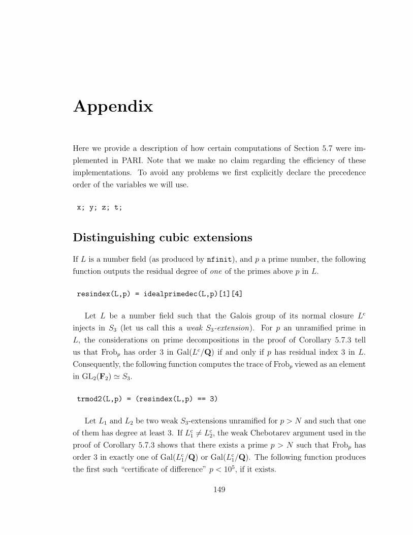
Appendix

Here we provide a description of how certain computations of Section 5.7 were im-

plemented in PARI. Note that we make no claim regarding the efficiency of these

implementations. To avoid any problems we first explicitly declare the precedence

order of the variables we will use.

x; y; z; t;

Distinguishing cubic extensions

If L is a number field (as produced by nfinit), and p a prime number, the following

function outputs the residual degree of one of the primes above p in L.

resindex(L,p) = idealprimedec(L,p)[1][4]

Let L be a number field such that the Galois group of its normal closure Lc

injects in S3 (let us call this a weak S3-extension). For p an unramified prime in

L, the considerations on prime decompositions in the proof of Corollary 5.7.3 tell

us that Frobp has order 3 in Gal(Lc/Q) if and only if p has residual index 3 in L.

Consequently, the following function computes the trace of Frobp viewed as an element

in GL2(F2) ' S3.

trmod2(L,p) = (resindex(L,p) == 3)

Let L1 and L2 be two weak S3-extensions unramified for p > N and such that one

of them has degree at least 3. If Lc1 6= Lc

2, the weak Chebotarev argument used in the

proof of Corollary 5.7.3 shows that there exists a prime p > N such that Frobp has

order 3 in exactly one of Gal(Lc1/Q) or Gal(Lc

1/Q). The following function produces

the first such “certificate of difference” p < 105, if it exists.

149

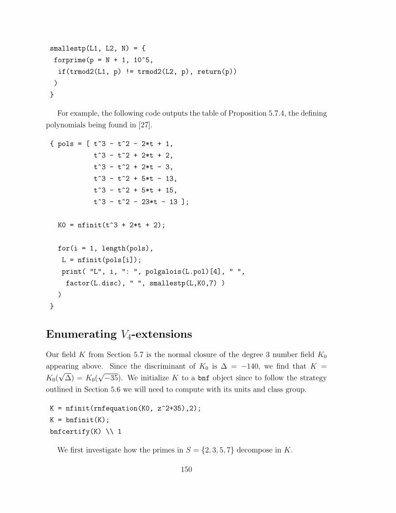
smallestp(L1, L2, N) =

forprime(p = N + 1, 10^5,

if(trmod2(L1, p) != trmod2(L2, p), return(p))

)

For example, the following code outputs the table of Proposition 5.7.4, the defining

polynomials being found in [27].

pols = [ t^3 - t^2 - 2*t + 1,

t^3 - t^2 + 2*t + 2,

t^3 - t^2 + 2*t - 3,

t^3 - t^2 + 5*t - 13,

t^3 - t^2 + 5*t + 15,

t^3 - t^2 - 23*t - 13 ];

K0 = nfinit(t^3 + 2*t + 2);

for(i = 1, length(pols),

L = nfinit(pols[i]);

print( "L", i, ": ", polgalois(L.pol)[4], " ",

factor(L.disc), " ", smallestp(L,K0,7) )

)

Enumerating V4-extensions

Our field K from Section 5.7 is the normal closure of the degree 3 number field K0

appearing above. Since the discriminant of K0 is ∆ = −140, we find that K =

K0(√

∆) = K0(√−35). We initialize K to a bnf object since to follow the strategy

outlined in Section 5.6 we will need to compute with its units and class group.

K = nfinit(rnfequation(K0, z^2+35),2);

K = bnfinit(K);

bnfcertify(K) \\ 1

We first investigate how the primes in S = 2, 3, 5, 7 decompose in K.

150

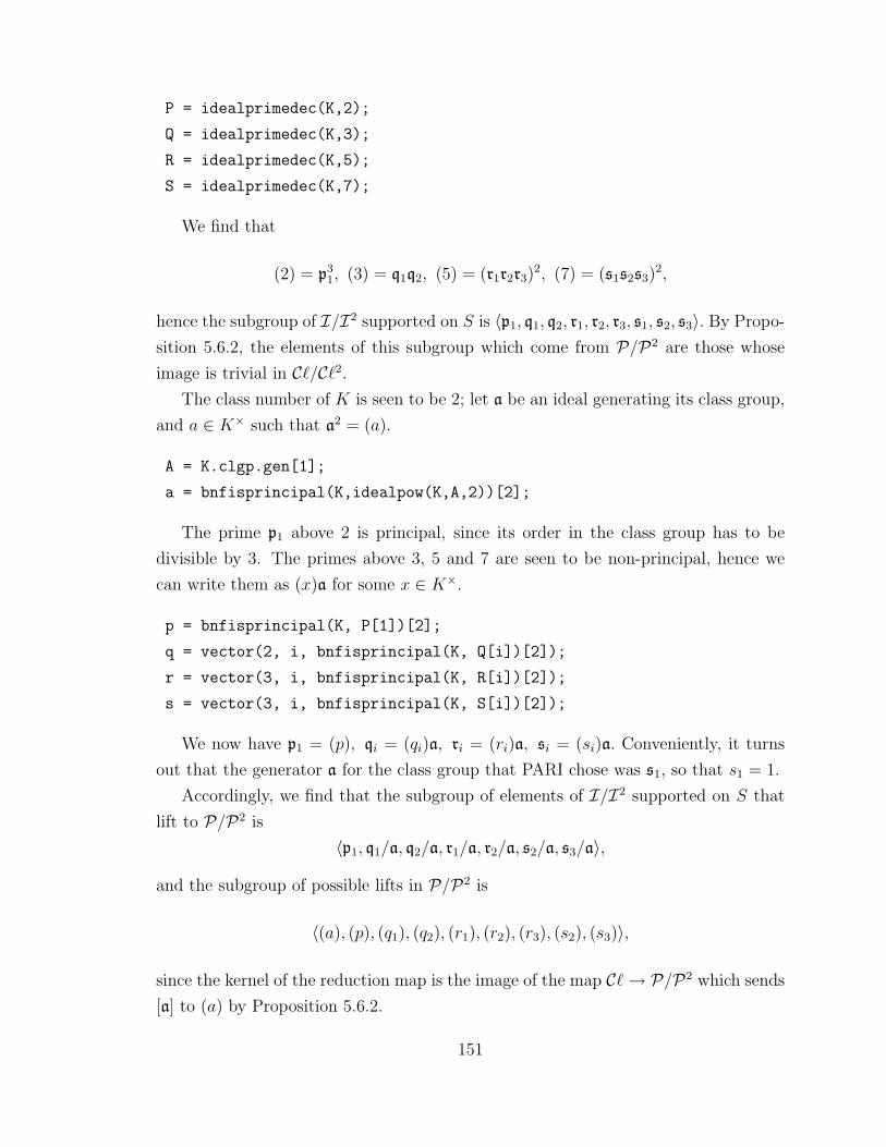
P = idealprimedec(K,2);

Q = idealprimedec(K,3);

R = idealprimedec(K,5);

S = idealprimedec(K,7);

We find that

(2) = p31, (3) = q1q2, (5) = (r1r2r3)2, (7) = (s1s2s3)2,

hence the subgroup of I/I2 supported on S is 〈p1, q1, q2, r1, r2, r3, s1, s2, s3〉. By Propo-

sition 5.6.2, the elements of this subgroup which come from P/P2 are those whose

image is trivial in C`/C`2.

The class number of K is seen to be 2; let a be an ideal generating its class group,

and a ∈ K× such that a2 = (a).

A = K.clgp.gen[1];

a = bnfisprincipal(K,idealpow(K,A,2))[2];

The prime p1 above 2 is principal, since its order in the class group has to be

divisible by 3. The primes above 3, 5 and 7 are seen to be non-principal, hence we

can write them as (x)a for some x ∈ K×.

p = bnfisprincipal(K, P[1])[2];

q = vector(2, i, bnfisprincipal(K, Q[i])[2]);

r = vector(3, i, bnfisprincipal(K, R[i])[2]);

s = vector(3, i, bnfisprincipal(K, S[i])[2]);

We now have p1 = (p), qi = (qi)a, ri = (ri)a, si = (si)a. Conveniently, it turns

out that the generator a for the class group that PARI chose was s1, so that s1 = 1.

Accordingly, we find that the subgroup of elements of I/I2 supported on S that

lift to P/P2 is

〈p1, q1/a, q2/a, r1/a, r2/a, s2/a, s3/a〉,

and the subgroup of possible lifts in P/P2 is

〈(a), (p), (q1), (q2), (r1), (r2), (r3), (s2), (s3)〉,

since the kernel of the reduction map is the image of the map C`→ P/P2 which sends

[a] to (a) by Proposition 5.6.2.

151

It follows that the subgroup B of K×/(K×)2 corresponding to exponent 2 exten-

sions of K unramified outside S is

B = O×/(O×)2 × 〈a, p, q1, q2, r1, r2, r3, s2, s3〉.

Here O× has rank 2, and O× = 〈−1〉 × 〈ε2, ε3〉. Hence B, as a vector space over F2,

has a basis consisting of

−1, ε2, ε3, a, p, q1, q2, r1, r2, r3, s2, s3.

eps = K.tufu;

gen = concat(eps, [a, p, q[1], q[2], r[1], r[2], r[3], s[2], s[3]]);

gen = nfbasistoalg(K, gen);

We now explicitly compute representatives in K× for the 212 elements of B.

drop(list) = if(length(list) <= 1, [], vecextract(list, "2.."))

products(list) =

if(list == [], [1],

tmp = products(drop(list)); concat(tmp, list[1]*tmp)

)

repr = products(gen);

To find all the subgroups B ⊂ B which are isomorphic to V4 as an F2[S3]-module,

we need to be able to decide when two elements of K× are equal in K×/(K×)2.

sqroot(d) =

fact = idealfactor(K, d);

id = 1;

for(i = 1, matsize(fact)[1],

if(fact[i,2] % 2 != 0, return(0),

id = idealmul(K, id, idealpow(K, fact[i,1], fact[i,2]/2))

152

)

);

\\ now (d) = id^2

fact = bnfisprincipal(K,id);

if(fact[1] == [1]~, return(0), rac = fact[2]);

\\ now (d) = (rac)^2, d = u*rac^2

u = nfeltdiv(K, d, nfeltpow(K, rac, 2));

fact = bnfisunit(K, u);

if(fact[3] == Mod(1,2), return(0)); \\ sign

v = 1;

for(i=1, 2,

if(fact[i] % 2 != 0, return(0),

v = v * K.fu[i]^(fact[i]/2);

)

);

\\ now x = v^2 rac^2

nfeltmul(K, v, rac)

For x, y ∈ K×, the following function returns an element z such that x = z2y if it

exists; else it returns 0.

congmodsquares(x,y) = sqroot(nfeltdiv(K,x,y))

By computing their iterates on the primitive element of K we identify the three

transpositions in G = Gal(K/Q) ' S3.

ord(g) =

pow = Mod(g, K.pol); id = Mod(z, K.pol); n = 1;

while(pow != id, pow = nfgaloisapply(K,g,pow); n++);

return(n)

153

G = nfgaloisconj(K);

tau = [];

for(i = 1, length(G), if(ord(G[i]) == 2, tau = concat(tau, [G[i]])))

We now search for all the subgroups B of type V4. They are the subsets of B of

the form 1, α, β, γ, where α, β, γ is an orbit for the action of G on K×/(K×)2

such that α · β = γ.

list = [];

for(i = 1, length(repr), alpha = repr[i];

\\ check if we already found a B containing alpha

found = 0;

for(j = 1, length(list), for(k = 1, 3,

if(congmodsquares(alpha, list[j][k]), found = 1)

) );

if(found, next);

\\ looks for transpositions fixing alpha

compt = 0;

for(j = 1, 3,

if( congmodsquares(alpha, nfgaloisapply(K, tau[j], alpha)),

compt++; fix = j

)

);

\\ |Orb| = 3 iff Stab contains a unique transposition

if( compt != 1, next );

\\ let tau[j], tau[k] be the two others

if( fix == 1, j = 2; k = 3 );

if( fix == 2, j = 1; k = 3 );

if( fix == 3, j = 1; k = 2 );

154

beta = nfgaloisapply(K, tau[j], alpha);

gama = nfgaloisapply(K, tau[k], alpha); \\ sic

\\ if alpha*beta = gama we found a new B

if( congmodsquares(nfeltmul(K, alpha, beta), gama),

list = concat(list, [[alpha, beta, gama]])

)

);

Now list contains 7 triples corresponding to the subgroups B of B of type V4, as

claimed in the proof of Proposition 5.7.5. For every corresponding extension L, we

look for a prime p > 7 such that Frobp has order 4 in Gal(L/Q).

smallestP(L, N) =

forprime(p = N + 1, 10^5, if(resindex(L,p) == 4, return(p)))

for(i = 1, length(list),

B = 49*list[i]; \\ for some reason PARI complains without the 49

alpha = B[1];

F = rnfinit(K, y^2 - alpha); \\ intermediate extension

beta = rnfeltup(F, B[2]);

F = nfinit(F.pol);

L = nfinit(rnfequation(F, x^2 - beta));

print("L", i, ": ", smallestP(L,7))

)

We find 19, 23 and 31, as claimed in the proof of Proposition 5.7.5.

155

156

Bibliography

[1] J. Achter. Detecting complex multiplication. In Computational aspects of alge-

braic curves, volume 13 of Lecture Notes Ser. Comput., pages 38–50. World Sci.

Publ., Hackensack, NJ, 2005.

[2] L. Adleman and M.-D. Huang. Counting points on curves and abelian varieties

over finite fields. Symbolic Comput., 32(3):171–189, 2001.

[3] M. Atiyah and I. Macdonald. Introduction to commutative algebra. Addison-

Wesley Publishing Co.

[4] B. Birch. How the number of points of an elliptic curve over a fixed prime field

varies. J. London Math. Soc., 43:57–60, 1968.

[5] N. Bourbaki. Algebre commutative, chapitre 8: dimension. Masson, Paris, 1983.

[6] C. Breuil, B. Conrad, F. Diamond, and R. Taylor. On the modularity of elliptic

curves over Q: wild 3-adic exercises. J. Amer. Math. Soc., 14(4):843–939, 2001.

[7] H. Cohen. Advanced topics in computational number theory, volume 193 of Grad-

uate Texts in Mathematics. Springer-Verlag, New York, 2000.

[8] C. Consani and J. Scholten. Arithmetic on a quintic threefold. Internat. J. Math.,

12(8):943–972, 2001.

[9] J. Conway, R. Curtis, S. Norton, R. Parker, and R. Wilson. Atlas of finite groups.

Oxford University Press, Eynsham, 1985.

[10] A. de Jong. Smoothness, semi-stability and alterations. Inst. Hautes Etudes Sci.

Publ. Math., (83):51–93, 1996.

[11] P. Deligne. Formes modulaires et representations `-adiques. In Seminaire Bour-

baki 1968/1969, Exp. 355, Lecture Notes in Mathematics, Vol. 179. Springer-

Verlag, Berlin, 1971.

157

[12] P. Deligne. Cohomologie des intersections completes. In SGA 7: Groupes de

monodromie en geometrie algebrique II, Lecture Notes in Mathematics, Vol. 340.

Springer-Verlag, Berlin, 1973.

[13] P. Deligne. La conjecture de Weil. I. Inst. Hautes etudes Sci. Publ. Math.,

(43):273–307, 1974.

[14] P. Deligne. SGA 412: Cohomologie etale, volume 569 of Lecture Notes in Mathe-

matics. Springer-Verlag, Berlin, 1977.

[15] P. Deligne and G. Lusztig. Representations of reductive groups over finite fields.

Ann. of Math. (2), 103(1):103–161, 1976.

[16] M. Deuring. On the zeta-function of an elliptic function field with complex mul-

tiplications. In Proceedings of the international symposium on algebraic number

theory, Tokyo & Nikko, 1955. Science Council of Japan, Japan, 1956.

[17] G. Faltings. Endlichkeitssatze fur abelsche Varietaten uber Zahlkorpern. Invent.

Math., 73(3):349–366, 1983.

[18] J.-M. Fontaine and Y. Ouyang. Theory of p-adic Galois representations. Springer.

In preparation.

[19] E. Freitag and R. Kiehl. Etale cohomology and the Weil conjecture, volume 13 of

Ergebnisse der Mathematik und ihrer Grenzgebiete (3). Springer-Verlag, Berlin,

1988.

[20] W. Fulton and J. Harris. Representation theory, a first course, volume 129 of

Graduate Texts in Mathematics. Springer-Verlag, New York, 1991.

[21] P. Griffiths and J. Harris. Principles of algebraic geometry. Wiley Classics Li-

brary. John Wiley & Sons Inc., New York, 1994.

[22] A. Grothendieck. Formule de lefschetz et rationalite des fonctions L. In Dix

exposes sur la cohomologie des schemas, volume 3 of Advanced Studies in Pure

Mathematics. North-Holland Publishing Co., Amsterdam, 1968.

[23] R. Hartshorne. Algebraic geometry, volume 52 of Graduate Texts in Mathematics.

Springer-Verlag, New York, 1977.

158

[24] F. Hirzebruch. Topological methods in algebraic geometry. Classics in Mathemat-

ics. Springer-Verlag, Berlin, 1995.

[25] K. Hulek, R. Kloosterman, and M. Schutt. Modularity of Calabi-Yau varieties.

In Global aspects of complex geometry, pages 271–309. Springer, Berlin, 2006.

[26] K. Ireland and M. Rosen. A classical introduction to modern number theory,

volume 84 of Graduate Texts in Mathematics. Springer-Verlag, New York, second

edition, 1990.

[27] J. Jones. Tables of number fields with prescribed ramification, June 2001.

http://math.asu.edu/~jj/numberfields/.

[28] N. Katz. On a certain class of exponential sums. J. Reine Angew. Math., 377:12–

17, 1987.

[29] N. Katz. Gauss sums, Klossterman sums, and monodromy groups, volume 116

of Annals of Mathematics Studies. Princeton University Press, Princeton, NJ,

1988.

[30] C. Khare. Modularity of Galois representations and motives with good reduction

properties. J. Ramanujan Math. Soc., 22(1):75–100, 2007.

[31] C. Khare and J.-P. Wintenberger. Serre’s modularity conjecture: the case of odd

conductors (I). Preprint, 2006.

[32] R. Kiehl and R. Weissauer. Weil conjectures, perverse sheaves and `-adic Fourier

transform, volume 42 of Ergebnisse der Mathematik und ihrer Grenzgebiete.

Springer-Verlag, Berlin, 2001.

[33] S. Kobayashi. Fixed points of isometries. Nagoya Math. J., 13:63–68, 1958.

[34] N. Korobov. Exponential sums and their applications, volume 80 of Mathemat-

ics and its Applications (Soviet Series). Kluwer Academic Publishers Group,

Dordrecht, 1992.

[35] J. Lagarias, H. Montgomery, and A. Odlyzko. A bound for the least prime ideal

in the Chebotarev density theorem. Invent. Math., 54(3):271–296, 1979.

[36] A. Lauder. Counting solutions to equations in many variables over finite fields.

Found. Comput. Math., 4(3):221–267, 2004.

159

[37] G. Laumon. Exponential sums and `-adic cohomology: a survey. Israel J. Math.,

120(part A):225–257, 2000.

[38] R. Livne. The average distribution of cubic exponential sums. J. Reine Angew.

Math., 375/376:362–379, 1987.

[39] R. Livne. Cubic exponential sums and Galois representations. In Current trends

in arithmetical algebraic geometry (Arcata, Calif., 1985), volume 67 of Contemp.

Math., pages 247–261. Amer. Math. Soc., Providence, RI, 1987.

[40] J.-F. Mestre. Courbes de Weil de conducteur 5077. C. R. Acad. Sci. Paris Ser.

I Math., 300(15):509–512, 1985.

[41] J. Milne. Etale cohomology, volume 33 of Princeton Mathematical Series. Prince-

ton University Press, Princeton, N.J., 1980.

[42] J. Milnor. Singular points of complex hypersurfaces. Annals of Mathematics

Studies, No. 61. Princeton University Press, Princeton, NJ, 1968.

[43] D. Mumford. Abelian varieties. Tata Institute of Fundamental Research Studies

in Mathematics, No. 5. Bombay, 1970.

[44] R. Murty. Congruences between modular forms. In Analytic number theory

(Kyoto, 1996), volume 247 of London Math. Soc. Lecture Note Ser., pages 309–

320. Cambridge Univ. Press, Cambridge, 1997.

[45] J. Neukirch. Class field theory, volume 280 of Grundlehren der Mathematischen

Wissenschaften. Springer-Verlag, Berlin, 1986.

[46] K. Ribet. Report on mod ` representations of Gal(Q/Q). In Motives (Seattle,

WA, 1991), volume 55 of Proc. Sympos. Pure Math., pages 639–676. Amer. Math.

Soc., Providence, RI, 1994.

[47] R. Rodrıguez and V. Gonzalez-Aguilera. Fermat’s quartic curve, Klein’s curve

and the tetrahedron. In Extremal Riemann surfaces (San Fransisco, 1995), vol-

ume 201 of Contemp. Math. Amer. Math. Soc., Providence, RI, 1997.

[48] B. Sagan. The symmetric group: representations, combinatorial algorithms, and

symmetric functions, volume 203 of Graduate Texts in Mathematics. Springer-

Verlag, New York, 2001.

160

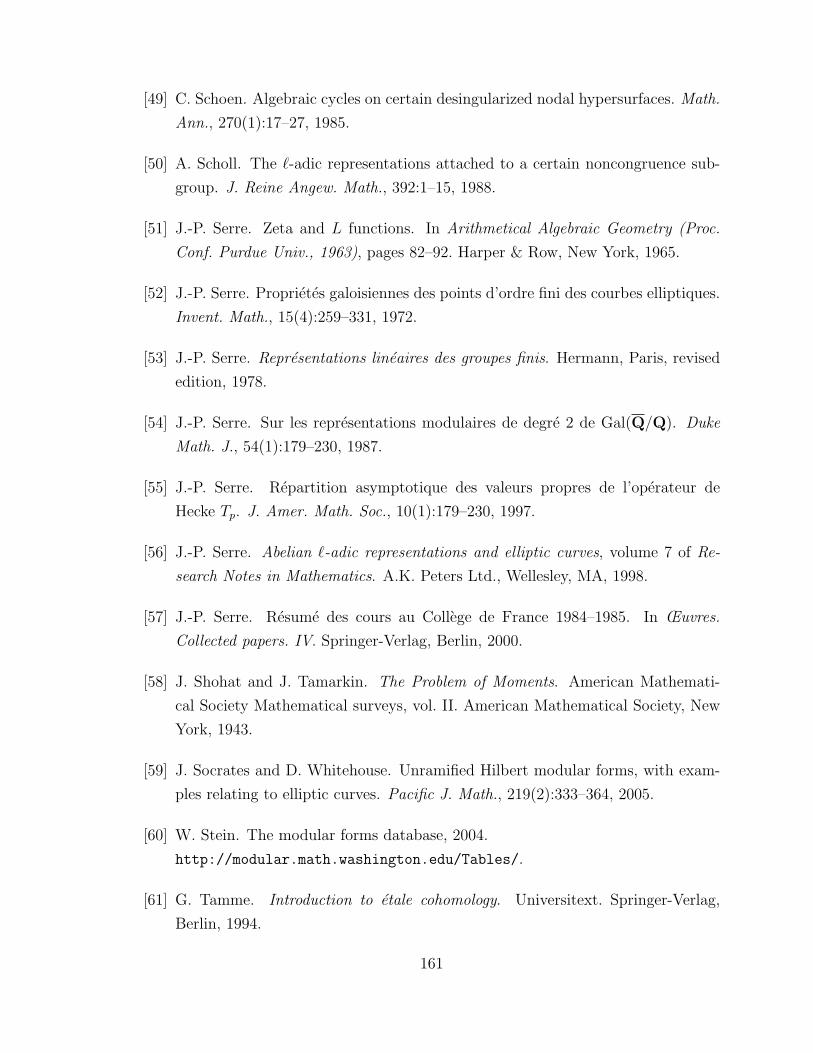
[49] C. Schoen. Algebraic cycles on certain desingularized nodal hypersurfaces. Math.

Ann., 270(1):17–27, 1985.

[50] A. Scholl. The `-adic representations attached to a certain noncongruence sub-

group. J. Reine Angew. Math., 392:1–15, 1988.

[51] J.-P. Serre. Zeta and L functions. In Arithmetical Algebraic Geometry (Proc.

Conf. Purdue Univ., 1963), pages 82–92. Harper & Row, New York, 1965.

[52] J.-P. Serre. Proprietes galoisiennes des points d’ordre fini des courbes elliptiques.

Invent. Math., 15(4):259–331, 1972.

[53] J.-P. Serre. Representations lineaires des groupes finis. Hermann, Paris, revised

edition, 1978.

[54] J.-P. Serre. Sur les representations modulaires de degre 2 de Gal(Q/Q). Duke

Math. J., 54(1):179–230, 1987.

[55] J.-P. Serre. Repartition asymptotique des valeurs propres de l’operateur de

Hecke Tp. J. Amer. Math. Soc., 10(1):179–230, 1997.

[56] J.-P. Serre. Abelian `-adic representations and elliptic curves, volume 7 of Re-

search Notes in Mathematics. A.K. Peters Ltd., Wellesley, MA, 1998.

[57] J.-P. Serre. Resume des cours au College de France 1984–1985. In Œuvres.

Collected papers. IV. Springer-Verlag, Berlin, 2000.

[58] J. Shohat and J. Tamarkin. The Problem of Moments. American Mathemati-

cal Society Mathematical surveys, vol. II. American Mathematical Society, New

York, 1943.

[59] J. Socrates and D. Whitehouse. Unramified Hilbert modular forms, with exam-

ples relating to elliptic curves. Pacific J. Math., 219(2):333–364, 2005.

[60] W. Stein. The modular forms database, 2004.

http://modular.math.washington.edu/Tables/.

[61] G. Tamme. Introduction to etale cohomology. Universitext. Springer-Verlag,

Berlin, 1994.

161

[62] J. Tate. Algebraic cycles and poles of zeta functions. In Arithmetica Algebraic

Geometry (Proc. Conf. Purdue Univ., 1963), pages 93–110. Harper & Row, New

York, 1965.

[63] R. Taylor. Galois representations. Ann. Fac. Sci. Toulouse Math. (6), 13(1):73–

119, 2004.

[64] R. Taylor and A. Wiles. Ring-theoretic properties of certain hecke algebras. Ann.

of Math. (2), 141(3):553–572, 1995.

[65] A. Weil. Numbers of solutions of equations in finite fields. Bull. Amer. Math.

Soc., 55:497–508, 1949.

[66] A. Wiles. Modular elliptic curves and Fermat’s last theorem. Ann. of Math. (2),

141(3):443–551, 1995.

162