exponential models for sequential...

Exponential Models for Sequential Data

John Lafferty

School of Computer Science

Carnegie Mellon University

Joint work with:

Doug Beeferman, Adam Berger

Andrew McCallum, Fernando Pereira

Acknowledgements:

Yoshua Bengio, Leon Bottou, Michael Collins,

Yann LeCun, Andrew Ng, Sebastian Thrun

Motivating Problem:

Segment & Annotate Data with Content Tags

ICML Workshop on Learning from Spatial and Temporal Data 1

Sequence Segmentation and Labeling

• Goal : mark up sequences with content tags

• Problem: overlapping dependencies on context

– long-distance dependencies

– multiple levels of granularity (e.g., words & characters)

– aggregate properties (e.g., layout, html)

– past and future observations

• Generative models that can represent such dependencies

quickly become computationally intractable

• I’ll focus on text, but similar problems in many other domains;

e.g., biological sequence analysis


Modeling Sequences

Standard tool is the hidden Markov Model (HMM).

· · · Yi−1 Yi Yi+1 · · ·

· · · Xi−1 Xi Xi+1 · · ·

P (X,Y) =∏

i P (Xi |Yi)P (Yi |Yi−1)

• Generative models, strong independence assumptions.

• Very widely used (genomics, natural language, information

extraction...)


Conditional Models

• Model p(label sequence y | observation sequence x) rather

than joint probability p(y,x)

• Allow arbitrary dependencies on the observation sequence x

• Still efficient (Viterbi, forward-backward) if dependencies

within the state sequence y are constrained

• Do not need to use states to model dependency on past and

future observations ⇒ smaller state space, easier to design


Using Exponential Models (MEMMs)

• Represent probability P (y′ |x, y) of new state given

observation and previous state as a product of “feature

effects”:

P (y′ | y, x) =1

Z(y, x)exp

∑

k

λk︸︷︷︸weight

fk(x, y, y′)︸︷︷︸feature

• Parameter estimation: Maximum likelihood or penalized

(regularized) ML via iterative scaling

• Good empirical success for labeling and information

extraction tasks (Rathnaparkhi, 1998; McCallum et al., 2000)


Outline

• Text Segmentation using Exponential Models

• The Label Bias Problem for State-Conditional Models

• Conditional Random Fields

• Experiments on Synthetic and Real Data


Text Segmentation

(BBL, 1999)

• Break up text stream into “semantically coherent” units

– Not completely well-defined

– Granularity depends on application

• Story segmentation: recover boundaries between “articles”

• Applications to video & audio retrieval

• Arises from temporal/sequential nature of data;

analogous problems for DNA sequences, many other domains


Modeling the “Topic” Adaptively

Some doctors are more skilled at doing the procedure

than others so it’s recommended that patients ask

doctors about their track record. People at high risk

of stroke include those over age 55 with a family history

or high blood pressure, diabetes and smokers. We urge

them to be evaluated by their family physicians and this

can be done by a very simple procedure simply by having

them test with a stethoscope for symptoms of blockage.


An Adaptive Language Model (Generative)

• First construct a standard, static (stationary) backoff trigram

model

ptri(w | w−2, w−1)

• Use this as a prior/default in a family of conditional

exponential models

pexp(w | H) =1

Z(H)exp

(∑

i

λifi(H,w)

)ptri(w | w−2, w−1)

where H ≡ w−N , w−W+1, . . . , w−1 is the word history .


An Adaptive Language Model (cont.)

• The features fi depend both on the word history H and the

word being predicted; assigned a weight λi.

• H is the previous 500-word context (sliding window)

• Here we use trigger features:

fi(H,w) ={

1 if si ∈ H and w = ti0 otherwise.


Sample Triggers

(s, t) eλ

residues, carcinogens 2.3

Charleston, shipyards 4.0

microscopic, cuticle 4.1

defense, defense 8.4

tax, tax 10.5

Kurds, Ankara 14.8

Vladimir, Gennady 19.6

education, education 22.2

music, music 22.4

insurance, insurance 23.0

Pulitzer, prizewinning 23.6

Yeltsin, Yeltsin 23.7

Russian, Russian 26.1

sauce, teaspoon 27.1

flower, petals 32.3

casinos, Harrah’s 42.8

(s, t) eλ

recent, recent 2.3

national, national 3.3

University, University 3.5

Doo, Chun 6.3

Soviet, Soviet 6.9

fraud, fraud 8.0

detergent, Tide 9.2

Carolco, Hoffman 9.7

Freddie, conventional 10.0

aluminium, smelter 10.4

officers, officers 11.0

records, records 11.5

merger, merger 11.6

proportionate, chances 15.6

nutrasweet, sweetener 18.4

waste, waste 20.7


Change Across Segment Boundaries

-0.05

0

0.05

0.1

0.15

0.2

0.25

-500 -400 -300 -200 -100 0 100 200 300 400 500

LRi = log

(pexp(wi |H)

ptri(wi | wi−2, wi−1)

)


Lexical Features

Broadcast news:

CNN’S richard blystone is here to tell us...

this is wolf blitzer reporting live from the white

house.

Newswire:

a texas air national guard fighter jet crashed

Friday in a remote area of southwest texas.

He was at home waiting for a limousine to take him

to los angeles airport for a trip to chicago.


The Learning Paradigm:

Feature Selection/Induction

• Goal: construct a probability distribution q(b |ω), where

b ∈ {yes,no} is the value of a random variable describing

the presence of a segment boundary in context ω.

• We consider distributions in the exponential family

Q(f, q0) =

{q(· |ω) : q(b |ω) =

1

Zλ(ω)eλ·f(ω) q0(b |ω)

}

λ · f(ω) = λ1f1(ω) + λ2f2(ω) + · · · λnfn(ω) .

• The gain of the candidate feature g is defined to be

Gq(g) = argmaxα (D(p ‖ q)−D(p ‖ qα,f)) .


First Features Selected for WSJ

currentposition +1 +2 +3 +4 +5-1-2-3-4-5

INCORPORATED

4.5−0.50 < LRi < 0

5.3CORPORATION

31.6SAYS

0.39MR.

0.07CLOSED

27.6SAID

2.9FEDERAL

6.8

SAID¬ SAID

2.7THE

0.36POINT

4.5LRi ≤ 0

4.5NAMED

14.2SEE

94.8 15

Sample Segmentations of Wall Street Journal


First Features Selected for CNNcurrentposition +1 +2 +3 +4 +5-1-2-3-4-5

C.

9.0I

0.61FRIDAY

9.93JOINS

2.26A

3.10−0.1 ≤ LRi < 0

3.4J.

7.76HAITI

5.95C.

7.910 < LRi < 0.05

1.85C.

2.06IT’S

0.55IN

1.7IS

0.59J.

0.1017

Sample Segmentations: WSJ/CNN


Evaluation: A Probabilistic Error Metric

Error is calculated as the probability Pµ that the reference and

hypothesized segmentations disagree between two randomly

chosen word positions:

okay false alarmmiss okay(b)(a) (c) (d)

Reference

segmentation

segmentation

Hypothesized

Words


Quantitative Segmentation Results

modelreferencesegments

hypoth.segments Pµ precision recall F-meas.

exp. model 9984 9543 0.12 60% 57% 58

random 9984 9984 0.32 12% 12% 12

all 9984 219,099 0.41 5% 100% 9

none 9984 0 0.57 0% 0% —

even 9984 9980 0.26 14% 12% 13%

(Note: Have also compared to HMMs, decision trees, and some

other methods.)


Modeling Temporal Structure

• This finesses the sequential/temporal nature of the problem:

Viewed as series of classification problems with simple

sequential decision rule

• Want explicit notion of time/state

• Represent probability P (yi |x, yi−1) of new state given

observation and previous state using features:

P (yi | yi−1, x) =1

Z(yi−1, x)exp(

∑

k

λk︸︷︷︸weight

fk(x, yi−1, yi)︸︷︷︸feature

)

• However, potential problem...


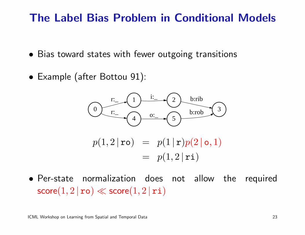
The Label Bias Problem in Conditional Models

• Bias toward states with fewer outgoing transitions

• Example (after Bottou 91):

0

1r:_

4r:_

2i:_

3

b:rib

5o:_ b:rob

p(1, 2 | ro) = p(1 | r)p(2 | o, 1)

= p(1, 2 | ri)

• Per-state normalization does not allow the required

score(1, 2 | ro) � score(1, 2 | ri)


Experiments on Synthetic Data

• Generate data according to mixture of first-order and second-

order hidden Markov Model (5 states, 26 outputs)

p(x,y) = (1− α) p1(x,y) + α p2(x,y)

• Train first-order models parameterized in the same way.

• As the data becomes more second order, the error rates

increase, as first-order models fail to fit higher-order data.


MEMM vs. HMM

0

10

20

30

40

50

60

0 10 20 30 40 50 60

ME

MM

Err

or

HMM Error

first orderdata

second orderdata


Proposed Solutions

1. Determinization: 0 1,4r:_2i:_

5o:_ 3

b:rib

b:rob

• not always possible

• state-space explosion

2. Fully-connected models: lack prior structural knowledge

3. Our solution: Conditional random fields (CRFs):

• Allow some transitions to “vote” more strongly than others

in computing state sequence probability

• Whole sequence rather than per-state normalization;

conditioned on entire input sequence.

• Convex likelihood function


Classical Notion of Random Field


Markov Property

p(XA |Xv, v 6∈ A) = p(XA |Xv, v ∈ ∂A)


Random Fields on Sequences:

Chains and Trees


Conditional Random Fields

Suppose there is a graphical structure to Y; i.e., graph G =

(V,E) such that Y = (Y1,Y2, . . . ,Y|V |).

A distribution p(Y |X) is a conditional random field in case,

when conditioned on X, the random variables Yv obey the

Markov property with respect to the graph:

p(Yv |X,Yw, w 6= v) = p(Yv |X,Yw, (w, v) ∈ E)


Tree-based Models

Assume underlying graph is a tree. Hammersley-Clifford

theorem says CRF is a Gibbs distribution:

pθ(y |x) ∝ exp

∑

e∈E,k

λk fk(e,y|e,x) +∑

v∈V,k

µk gk(v,y|v,x)


CRFs for Sequences

• The state sequence is a Markov random field conditioned on

the observation sequence

• Model form: p(y |x)∝exp∑T

t=1

[ ∑j λjfj(yt, yt−1 |x, t)

+∑

k µkgk(yt |x, t)

]

• Features:

– fj represent the interaction between successive states,

conditioned on the observations

– gk represent the dependence of a state on the observations

• Dependence on entire observation sequence


A Special Case: From HMMs to CRFs

HMM:

p(y |x) ∝∏T

t=1 p(yt | yt−1)p(xt | yt)yi−1 yi

xi

MEMM:

p(y |x) =∏T

t=11

Zyt−1,xtexp

[ ∑j λjfj(yt, yt−1)

+∑

k µkgk(yt, xt)

] yi−1 yi

xi

CRF:

p(y |x) = 1Zx

∏Tt=1 exp

[ ∑j λjfj(yt, yt−1)

+∑

k µkgk(yt, xt)

] yi−1 yi

xi

Discriminative “Boltzmann chains” (Saul and Jordan; MacKay, 1996)


Efficient Estimation

Marginals and normalizing constant can be computed efficiently

using dynamic programming

Matrix notation:

Mi(y′, y |x) = exp (Λi(y

′, y |x))

Λi(y′, y |x) =

∑k λk fk(ei,Y|ei

= (y′, y),x) +∑

k µk gk(vi,Y|vi= y,x)

where ei is the edge with labels (Yi−1,Yi) and vi is the vertex

with label Yi.

Normalization (partition function):

Zθ(x) = (M1(x)M2(x) · · ·Mn+1(x))start,stop


Forward-Backward Calculations

• Probability of label Yi = y, given observation sequence x:

Probθ(Yi = y |x) =αi(y |x)βi(y |x)

Zθ(x)

αi(x) = αi−1(x)Mi(x)

βi(x)> = Mi+1(x)βi+1(x)

• Training requires forward-backward (unlike for HMMs)

• Complexity same as standard Baum-Welch, even with

“global” features.


Iterative Scaling

Update equations:

δλk =1

Slog

Efk

Efk

, δµk =1

Slog

Egk

Egk

where

Efk =∑

x

p(x)n+1∑

i=1

∑

y′,y

fk(ei,y|ei= (y′, y),x) ×

αi−1(y′ |x)Mi(y

′, y |x)βi(y |x)

Zθ(x)

(and similarly for Egk)


Recall: MEMM vs. HMM

0

10

20

30

40

50

60

0 10 20 30 40 50 60

ME

MM

Err

or

HMM Error


CRF vs. HMM

0

10

20

30

40

50

60

0 10 20 30 40 50 60

CR

F E

rror

HMM Error


MEMM vs. CRF

0

10

20

30

40

50

60

0 10 20 30 40 50 60

ME

MM

Err

or

CRF Error


CRF vs. HMM

0

5

10

15

20

25

30

35

40

0 5 10 15 20 25 30 35 40

CR

F E

rror

HMM Error


MEMM vs. CRF

0

5

10

15

20

25

30

35

40

0 5 10 15 20 25 30 35 40

ME

MM

Err

or

CRF Error


MEMM vs. HMM

0

5

10

15

20

25

30

35

40

0 5 10 15 20 25 30 35 40

ME

MM

Err

or

HMM Error


Experiments on Text

UPenn tagging task: 45 tags (syntactic), 1M words training

DTThe

NNasbestos

NNfiber ,,

NNcrocidolite ,,

VBZis

RBunusually

JJresilient

INonce

PRPit

VBZenters

DTthe

NNSlungs ,,

INwith

RBeven

JJbrief

NNSexposures

TOto

PRPit

VBGcausing

NNSsymptoms

WDTthat

VBPshow

RPup

NNSdecades

JJlater ,,

NNSresearchers

VBDsaid


Sample Results on Penn Data

error oov oov error

HMM 5.69% 5.45% 45.99%

MEMM 6.37% 5.45% 54.61%

CRF 5.55% 5.45% 48.05%


Results with Spelling Features

using spelling features

error oov error error ∆ oov error ∆

HMM 5.69% 45.99%

MEMM 6.37% 54.61% 4.81% -25% 26.99% -50%

CRF 5.55% 48.05% 4.27% -24% 23.76% -50%


Future Directions

• Tree-structured random fields for hierarchical parsing

• Feature selection and induction: automatically choose the fk

and gk functions (efficiently)

• Train to maximize per-symbol likelihood∏

i Prob(yi |x)

(not pseudo-likelihood)

• Numerical methods to accelerate convergence

(e.g. quasi-Newton, hybrid IS and conjugate gradient)

• Theoretical bounds on performance


Summary

• Conditional sequence models have the advantage of allowing

complex dependencies among input features

• May be prone to the label bias problem

• CRFs are an attractive modeling framework that:

– Discriminatively model sequence annotations

– Allow non-local features

– Avoid label bias through global normalization

– Have efficient inference & estimation algorithms


exponential models for sequential...

Documents