exploring the energy landscape

© M. S. Shell 2012 1/14 last modified 4/12/2012

Exploringtheenergylandscape ChE210D

Today's lecture: what are general features of the potential energy surface and

how can we locate and characterize minima on it

Derivatives of the potential energy function

Forces

For any atomic configuration, we can compute the force acting on each atom from the negative

energy derivative with respect to the particle coordinates:

��,� = −�� ,� = −��

�� ,� = −��

��

In shorthand notation,

�� = −��

�

Alternatively,

�� = −∇�� That is, the force stems from the gradient of the potential energy.

We can simplify this expression if our potential energy function is built from pairwise interac-

tions,

�� =��

We have that:

�� = �� − �� + �� − �� + �� − ��

Consider computing the force on atom �. There are − 1 terms in the pairwise summation

that include the coordinates of atom ". Thus the energy derivative with respect to �� is:

��,� = − ��

= − ��

�#�


= −��

�� #�

Using the definition of ��,

2�� = 2�� − ��

�� =

�� − ��

Hence,

��,� = −�� − ��

�� #�

Doing the same for the � and � coordinates,

�� =��

�� #�

where

�� = � − � For example, if our pair potential is the so-called soft-sphere interaction,

�� = % & �'()*

where + is a positive integer, then

�� =�� ,−+%'

*��)*)-.�#�

Simplifying,

�� = −+�� /% &

��'(

)*0

�#�

Notice that the force acting on atom " due to atom 1 is just the negative of the force acting on

atom 1 due to atom ", since

�� = −��2


In simulation, we typically maintain an (N,3) array of forces. A typical way to implement pair-

wise force and potential energy calculation in computer code is the following:

set the potential energy variable and elements of t he force array equal to zero loop over atom i = 1 to N – 1 loop over atom j = i+1 to N calculate the pair energy of atoms i and j add the energy to the potential energy variable calculate the force on atom i due to j add the force to the array elements for atom i subtract the force from the array elements for at om j

Second derivatives and the Hessian

The curvature of the potential energy function surrounding a given atomic configuration � is

given by second derivatives. There are 3 × 3 different second derivatives, attained by

cross-permuting different particle coordinates. We typically write the second derivatives as a

matrix called the Hessian:

5�� =

67777778 �� -�

�� - �- ⋯ ��

�- �� - �-

�� - �- ⋯ ��

�- ��⋮ ⋮ ⋱ ⋮ �� -

�� - ⋯ ��

�� <======>

The Hessian is important in distinguishing potential energy minima from saddle points, as

discussed in greater detail below. It can be a memory-intensive matrix to compute in molecular

simulation, as the number of elements is 9 �.

The energy landscape

Basic definition and properties

The potential energy function �� defines all of the thermodynamic and kinetic properties of

a classical atomic system. We can think of this function as being plotted in a high-dimensional

space where there are 3 axes, one for each coordinate of every atom. An additional axis

measures the potential energy, and we call the projection of the potential energy function in

3 + 1 dimensional space as the potential energy landscape (PEL).

Though we cannot visualize the PEL directly, the following schematic shows some features of it:


Stationary points correspond to the condition where the slope of the PEL is zero:

∇�� = @

This is shorthand for the following simultaneous conditions:

�� = 0 ��

�� = 0 ��

�� = 0" = 1,2, … ,

Notice that these equations imply that the net force acting on each particle is zero:

�� = 0

Therefore, the stationary points correspond to mechanically stable configurations of the atoms

in the system.

There are two basic kinds of stationary points:

• For minima, the curvature surrounding the stationary point is positive. That is, any

movement away from the point increases the potential energy.

• For saddles, one can move in one or more directions around a stationary point and ex-

perience a decrease in potential energy.

Scaling of the number of minima and saddle points

PELs contain numerous stationary points. It can be shown [Stillinger, Phys Rev E (1999); Shell et

al, Phys Rev Lett (2004)] that both the number of minima and saddle points grow exponentially

with the number of atoms:

numberofminima~ exp' �

particle coordinates, �

�� local minima

saddle point basin

global minimum


numberofsaddlepoints~expT �

where ' and T are system-specific constants but independent of the number of atoms.

The implication of these scaling laws is that it is extraordinarily difficult to search exhaustively

for all of the minima for even very small systems (~100 atoms), since their number is so great.

By extension, it is extremely challenging to locate the global potential energy minimum, that is,

the set of particle coordinates that gives the lowest potential energy achievable.

The following figure shows a disconnectivity graph for a system of just 13 Lennard-Jones atoms

in infinite volume, taken from [Doye, Miller, and Wales, J. Chem. Phys. 111, 8417 (1999)].

The horizontal axis marks the potential energy and the lines show the connectivity of different

minima. To move from one minimum to another, one must travel the path formed when the

lines extending from two minima connect to a common energetic point. This small system has

1467 distinct potential energy minima. These results were generated using an advanced and

computationally-intensive minima-finding algorithm.

Relevance of finding minima

Why should we care to find PEL minima?


• Mechanically stable molecular structures can be identified. When examining conforma-

tional changes within a molecule, minima give the distinct conformational states possi-

ble. For changes among many molecules, the minima provide the basic structures asso-

ciated with physical events in the system (e.g., binding). Both can often be compared

with experiment.

• Differences in the energies of different minimized structures provide a first-order per-

spective on the relative populations of these (neglecting entropies). Again, this can be

compared to experiment and often is an important force field diagnostic.

• Initial structures in molecular simulations often need to be “relaxed” away from high-

energy states. Minimization can take an initial structure and remove atomic overlaps or

distorted bond and angle degrees of freedom.

Locating local energy minima

Problem formulation

If we are anywhere within the basin of a minimum, we can define a steepest descent protocol

that takes us to the minimum:

� U = −∇�

��lim U → ∞) = ��(�) Here, U is a fictitious time-like variable. The solution to this first order differential equation in

the limit that U → ∞ is the set of coordinates at a minimum min� . Here, we essentially follow

the forces down the potential energy surface until we reach its bottom—the velocities vectors

of each atom follow the negative forces. In a two-dimensional contour plot of energies (as a

function of coordinates), this would look like:


The steepest descent protocol is equivalent to an instantaneous quench of a system to absolute

zero: we continuously remove energy from the system until we cannot remove any more.

Line searches

It is very inefficient to implement the above equation because one must take U to infinity, and

because the closer we get to the minimum, the slower we are to converge due to the fact that

the forces grow increasingly small. A number of much more efficient methods are available.

These typically use a so-called line search as a part of the overall approach. A line search simply

says to find a minimum along one particular direction in coordinate space, X�. In two dimen-

sions,

The procedure for a line search is broken into two parts.

1. Start with an initial set of coordinates Y� and a search direction X�, chosen to be in the

downhill direction of the energy surface.

2. Let -� = Y�. Then, find two more coordinates �� = Y� + ZX� and [� = Y� + 2ZX� by

taking small steps Z along the search direction. Z should be chosen to be small relative

to the scales of energy changes relative to particle coordinates.

3. Is �([�) > �(��)? If so, the three coordinates bracket a minimum and we should

move to the next part of the algorithm.

4. If not, we need to keep searching along this direction. Let -� ← �� , �� ← [�, and [� ← �� + ZX�. Go back to step 3.

The second part of the algorithm consists of finding the minimum once we’ve bracketed it. One

possibility is to bisect pairs of coordinates:

1. Find a new coordinate ̂�. If |-� − ��| > |�� − [�|, pick ̂� = -� (-� + ��). Otherwise,

pick ̂� = -� (�� + [�).

X�


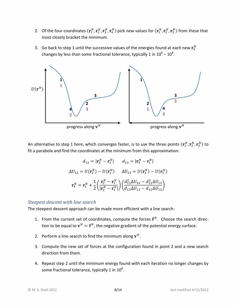
2. Of the four coordinates (-�, �� , [� , ̂�) pick new values for (-�, ��, [�) from these that

most closely bracket the minimum.

3. Go back to step 1 until the successive values of the energies found at each new ̂�

changes by less than some fractional tolerance, typically 1 in 106 – 10

8.

An alternative to step 1 here, which converges faster, is to use the three points (-�, �� , [�) to

fit a parabola and find the coordinates at the minimum from this approximation:

-� = |�� − -�| -[ = |[� − -�| Δ�-� = �(��) − �(-�)Δ�-[ = �([�) − �(-�) ̂� = -� + 12a �� − -�|�� − -�|b a -[� Δ�-� − -�� Δ�-[ -[Δ�-� − -�Δ�-[b

Steepest descent with line search

The steepest descent approach can be made more efficient with a line search:

1. From the current set of coordinates, compute the forces ��. Choose the search direc-

tion to be equal to X� = ��, the negative gradient of the potential energy surface.

2. Perform a line search to find the minimum along X�.

3. Compute the new set of forces at the configuration found in point 2 and a new search

direction from them.

4. Repeat step 2 until the minimum energy found with each iteration no longer changes by

some fractional tolerance, typically 1 in 108.

progress along X�

�(�) 1

1

3

2

3 4

2

progress along X�

1

3

3 2

1 4

2


Conjugate-gradient method

For long, narrow valleys in the PEL, the steepest descent + line search method results in a large

number of zigzag-type motions as one approaches the minimum. This is because the approach

continuously overcorrects itself when computing the new search direction with each iteration

(new line search). Instead, a more efficient approach is to use the conjugate gradient (CG)

method.

The CG approach differs only in the choice of a new search direction with each iteration in step

3. Like the steepest descent + line search approach, we use the gradient of the energy surface.

In addition, however, we use the previous search direction as well. The CG method chooses

search directions that are conjugate (perpendicular) to previous gradients found. A new search

direction at the "th iteration is found using

X�� = �� + c�X�)-�

with

c� = �� ⋅ ��)-� ⋅ ��)-�

Here, the dot product signifies the 3N-dimensional vector multiplication:

�� ⋅ �� = ��,-� + ��,-� + ��,-� + ��,�� +⋯+ ��,��

For +-dimensional quadratic functions, the CG approach converges exactly to the minimum in +

iterations (e.g., + line search operations).

An alternative equation for c is typically used in molecular modeling, as it has better conver-

gence properties:

c� = (�� − ��)-� ) ⋅ ��)-� ⋅ ��)-�


Newton and Quasi-Newton methods

Location of minima can be enhanced by using second derivative information. Consider the PEL

in the vicinity of a minimum. For the sake of simplicity, we will consider a one-dimensional

function �(�). We can Taylor expand �(�) and its derivative to second order:

�(�) = �(�Y) + (� − �Y) �(�Y) � + (� − �Y)�2 ��(�Y) �� …

�(�) � = �(�Y) � + (� − �Y) ��(�Y) �� …

Neglecting higher terms, we can solve for the point at which the derivative is zero:

� = �Y − a �(�Y) � ba ��(�Y) �� b)-

For quadratic functions, this relation will find the minimum after only a single application. For

other functions, this equation defines an iterative procedure whereby the minimum can be

located through successive applications of it (each time the function being approximated as

quadratic):

��e- = �� − a �(��) � ba ��(��) �� b)-

This is the Newton-Raphson iteration scheme for finding stationary points. The above proce-

dure will converge to both minima and saddle points. To converge to minima, one must first

move to a point on the PEL where the energy landscape has positive curvature in every direc-

tion.

For multidimensional functions �(�) the update equation above involves an inverse of the

Hessian matrix of second derivatives:

�e-� = �� + �� ⋅ 5�)-

To implement this method in simulation requires computation of the 3 × 3 Hessian matrix

and its inverse with each iteration step. For even small systems, this task can become compute-

and memory-intensive.

To remedy these issues, several quasi-Newton methods are available. The distinctive feature

of these approaches is that they generate approximations to the inverse Hessian; upon each

iteration, these approximations grow increasingly accurate. These approximations are generat-

ed from the force array. The most popular of these in use with molecular modeling methods is


the Limited Broyden-Fletcher-Goldfarb-Shanno (LBFGS) approach. Implementations of this

method can be found at online simulation code databases.

In general, Newton and quasi-Newton methods are more accurate and efficient than the

conjugate gradient approach; however, both are widely used in the literature.

Locating global energy minima

Methods to find global potential energy minima are actively researched and have important

applications in crystal and macromolecular structure prediction. The global minimum problem

is much more challenging as it requires a detailed search of the entire PEL and it is difficult if

not impossible to know a priori when the global minimum has been found (unless the entire

surface has been explored exhaustively).

Typically global-minimizers combine local minimization with various other methods to selec-

tively explore low-energy regions of the PEL and with bookkeeping routines to remember which

parts have been searched and what low-energy configurations have been found. This search is

usually partially stochastic in nature, often leveraging the molecular dynamics and Monte Carlo

techniques we will discuss in later lectures.

Normal mode analysis

For minima

Consider the PEL in the vicinity of a minimum. Let’s write the coordinates of all the atoms

about this minimum be

Y�

If we consider very small perturbations about these coordinates,

� = Y� + Δ�

we can Taylor expand the potential energy to second order. That is, we can perform a harmon-

ic approximation to the PEL about a minimum:

�(�) = �(Y�) + Δ�-�2 ��(Y�) �-� + Δ�-Δ�-2 ��(Y�) �- �- +⋯+ Δ��2 ��(Y�) ��

Notice that all of the first-order terms in the Taylor expansion are zero by the fact that �(Y�) is

a minimum. A shorter way of writing this is in matrix form using the Hessian:


Δ� = 12677778Δ�-Δ�-Δ�-Δ��⋮Δ��<=

===>f

67777778 �� -� �� - �- ⋯ �� - �� - �- �� - �- ⋯ �� - ��⋮ ⋮ ⋱ ⋮ �� - �� - ⋯ �� <=

=====>

677778Δ�-Δ�-Δ�-Δ��⋮Δ��<=

===>

which can be written in more compact form:

� = �Y + 12gf5g

where �Y = �(Y�) and g = Δ�. Keep in mind that the Hessian is evaluated at Y�.

We can use a trick of mathematics to simplify the analysis, by diagonalizing the Hessian matrix 5. Notice that 5 is a symmetric matrix, since the order in which the second derivatives are

taken doesn’t matter. That property means that we can write

5 = hfih

where i is a diagonal matrix of eigenvalues:

i = jk- 0 ⋯ 00 k� ⋯ 0⋮ ⋮ ⋱ ⋮0 0 ⋯ k�l and h is a matrix whose rows are eigenvectors of 5.

Then,

� = �Y + 12gfhfihg

= �Y + 12 (hg)fi(hg) = �Y + 12 mfim

In the last line, we defined a new set of 3 coordinates, instead of (g), that consists of linear

combinations of the atomic positions:

m = hg = h� − hY�


Physically, the new coordinates m correspond to projecting the atomic positions on a new set of

axes given by the eigenvectors of the Hessian.

Using the above Taylor expansion, the fact that i is a diagonal matrix means that the energy is

a simple a sum of 3 independent harmonic oscillators along the new directions m:

� = �Y + 12�k�U��[��n-

The physical interpretation of this result is the following. Starting from the minimum and at low

temperatures, the system oscillates about Y�. The eigenvectors of 5 give the normal modes

along which the system fluctuates, that is, the directions and collective motions of all of the

atoms that move in harmonic fashion for each oscillator. There are 3 of these modes corre-

sponding to the 3 eigenvectors.

The eigenvalues give the corresponding force constants and can be related to the frequencies

of fluctuations. If all atomic masses are the same, o, then

p� = qk� o⁄

In the case that the atomic masses differ, a slightly more complicated equation is used [Case,

Curr. Op. Struct. Biol. 4, 285 (1994)].

Regarding the eigenvalues,

• All will be positive or zero, since the energy must increase as one moves away from the

minimum. Thus, the frequencies are all real.

• If the system has translational symmetry (i.e., atoms can collectively be moved in the x,

y, and z directions without a change in energy), then three of the eigenvalues will be ze-

ro.

• If the system also has rotational symmetry (i.e., atoms can be collectively rotated about

the x, y, and z axes), then an additional three eigenvalues will be zero.

The spectrum of different normal mode frequencies informs one of motions on different

timescales:

• High-frequency modes signify very fast degrees of freedoms. The corresponding

eigenmodes typically correspond to bond stretching motions, if present. High-

frequency modes tend to be localized, i.e., involving only a few atoms.


• Low-frequency modes indicate slow degrees of freedoms. These modes tend to be col-

lective, involving the cooperative movement of many atoms.

For higher-order stationary points

Minima in the PEL are not the only points that satisfy the relation:

∇�(�) = 0

Saddle points are also defined by this condition. At a saddle point, the slope of the PEL is zero

but there exists at least one direction that will correspond to a decrease in the energy of a

system.

Recall that the PEL is a hypersurface in 3 + 1 dimensional space. This means that, at any

point on the PEL, there are 3 orthogonal directions that we can take. As a result, saddles can

be categorized by the number of directions that lead to a decrease in potential energy, called

the saddle order. First order saddles have one direction of negative curvature, second have

two, and so on and so-forth. A zeroth order saddle is a minimum and a 3 th order saddle is a

maximum.

An identical Taylor-expansion and normal mode analysis can be performed at a saddle point in

the potential energy surface:

• Unlike minima, saddles will have one or more eigenvalues of the Hessian that are nega-

tive. These correspond to a decrease in the potential energy as one moves away from

the saddle point.

• The corresponding eigenvectors give the saddle directions that result in this energy de-

crease.

• The number of negative eigenvalues gives the order of a saddle.

Such considerations can be useful when examining activated processes and barrier-crossing

events in molecular systems.

exploring the energy landscape

Documents