at SciVerse ScienceDirect

Environmental Pollution 166 (2012) 65e74

Contents lists available

Environmental Pollution

journal homepage: www.elsevier .com/locate/envpol

Exploring the applicability of future air quality predictions based on synopticsystem forecasts

Yuval a,*, David M. Broday a, Pinhas Alpert b

aDepartment of Civil and Environmental Engineering, Technion-Israel Institute of Technology, Haifa 32000, IsraelbDepartment of Geophysics and Planetary Sciences, Tel Aviv University, Tel Aviv, Israel

a r t i c l e i n f o

Article history:Received 23 October 2011Received in revised form27 February 2012Accepted 6 March 2012

Keywords:Air quality managementClimate changeSynoptic classification

* Corresponding author.E-mail address: lavuy@tx.technion.ac.il ( Yuval).

0269-7491/$ e see front matter � 2012 Elsevier Ltd.doi:10.1016/j.envpol.2012.03.010

a b s t r a c t

For a given emissions inventory, the general levels of air pollutants and the spatial distribution of theirconcentrations are determined by the physiochemical state of the atmosphere. Apart from the trivialseasonal and daily cycles, most of the variability is associated with the atmospheric synoptic scale. Asimple methodology for assessing future levels of air pollutants’ concentrations based on synopticforecasts is presented. At short time scales the methodology is comparable and slightly better thanpersistence and seasonal forecasts at categorical classification of pollution levels. It’s utility is shown forair quality studies at the long time scale of a changing climate scenario, where seasonality and persis-tence cannot be used. It is demonstrated that the air quality variability due to changes in the pollutionemissions can be expected to be much larger than that associated with the effects of climatic changes.

� 2012 Elsevier Ltd. All rights reserved.

1. Introduction

Numerous chemicals introduced into the atmosphere by naturaland anthropogenic sources have harmful effects on living organ-isms and may damage different aspects of the environmentthrough various processes on many time scales (Seinfeld andPandis, 1998). The adverse effects of air pollutants on humanhealth arewell known (e.g., World Health Organization, 2006; Popeet al., 1995; Schwartz and Dockery, 1992) and short term predictionof their concentrations is important in cases where they may reachdeleterious levels. Long term predictions of air quality are impor-tant for better management of the air resources and for estimationsof their possible long term impacts on the public’s health and onthe environment (Vallero, 2007).

Ambient air quality is closely linked to the prevailing weatherconditions (Seinfeld and Pandis, 1998). Most of the meteorologicalvariables depend to a large extent on the dominating atmosphericconfiguration at the synoptic scale and thus the synoptic patternsare associated with the quality of the air (Ganor et al., 2010; Chenet al., 2008; Cheng et al., 2007a; Tanner and Law, 2002;Triantafyllou, 2001). The link between the prevailing meteorologyand the quality of the air is at many levels. At the small spatialscales, the wind’s direction determines where local emissions willgo. The local wind speed and the nature of the atmospheric

All rights reserved.

stratification determine a pollutant’s dispersion around the mainadvection axis. Local sun radiation intensity (function of cloudcover), temperature and humidity determine the rates of chemicalreactions and transformations affecting the emissions. Large scaleatmospheric flows dictate transboundary transport of pollutants,with their composition usually strongly affected by ageingprocesses (Vallero, 2007). Al these meteorological conditionsdepend to a large extent on the type of synoptic system dominatinga region and thus, the synoptic systems provide very useful infor-mation for predicting the air quality. The effects of local factors liketopography, urbanisation and sea breeze cannot be neglectedthough, and they are superimposed on the synoptic scale condi-tions (Tanner and Law, 2002; Triantafyllou, 2001). The synopticsystem dominating a region at a certain time is usually definedusing the regional pressure and temperature fields, which aredescribed by data observations (Pearce et al., 2011; Cheng et al.,2007a; Alpert et al., 2004). For that purpose, point-wise data canbe processed and classified by a completely automated mathe-matical scheme (Pearce et al., 2011; Cheng et al., 2007a), or bya manual or semi-automatic procedure based on a training set ofspatial maps classified by experts (Alpert et al., 2004).

Due to the complexity of the processes governing air quality, airpollution prediction is a tough challenge. The difficulties lie in thecomplication of atmospheric photochemistry and the uncertaintiesdue to the inaccuracies in emission inventories, in addition to theuncertainties associated with the forecast of the atmospheric state.Even the state of the art of chemical transport models requireintegration of data observations in order to achieve reasonable

640

680

720

N

Haifa

Tel Aviv

Yuval et al. / Environmental Pollution 166 (2012) 65e7466

outputs for short term predictions (Carmichael et al., 2008).Moreover, use of chemical transport models becomes computa-tionally prohibitive for studies at the very long time scales.

This study presents a very simple alternative methodology forassessing future air pollutant levels, based on forecasted synopticsystems. The use of photochemical model is obviated but the tradeoff may be a reduced accuracy. Themethod does compare well withthe simple seasonal and persistence forecasts benchmark methodsfor short termpredictions. However, unlike these benchmarks it canbe utilised for studying the long term impacts of climatic changes onfuture air quality, based on existing climate model outputs.

2. Data

A 16 years database (1991e2006) of daily classification tosynoptic systems of the 12:00 UTC eastern Mediterranean NCEPdata was developed and provided by Alpert et al. (2004). A corre-sponding database for 1950e2099 was also provided based on theECHAM4/OPYC3 global climate model output (Roeckner andCoauthors, 1996; Chou et al., 2006). The ECHAM4/OPYC3 isa coupled ocean-atmosphere model. Its control run until 1990 wasbased on the observed CO2 and other greenhouse gasses emissions.Since 1990, the model was run according to input adapted from theIPCC Special Report on Emissions Scenarios scenario B2, wheredynamics of technological changes continue along the historicaltrends (IPCC, 2007). The synoptic system classification is based ona semi-objective classification of geopotential height, temperatureand the horizontal wind components at the 1000 hPa level. Alpertet al. (2004) defined 19 synoptic systems characteristic to theeastern Mediterranean, which can be lumped into six groups. Thesystems names and their group affiliations are given in Table 1.

The air quality data were observed by the air quality monitoringnetworks in the Haifa, Gush Dan and the southern coast areas ofIsrael (Fig. 1). The network in Haifa consists of 20 stations. Deploy-ment of the monitoring network commenced during 1985 but thenumber of stations has stabilised only since 2002. This studyconsiders the 2002e2006 data of SO2, NO2, O3, and PM10 formost of

Table 1A list of the synoptic systems, their synoptic system group affiliations and theseasons in which they are most frequent. The synoptic systems definitions and thegroup affiliation follow Alpert et al. (2004).

SystemNo.

System name Group Season

1 Red Sea Trough with the Easternaxis

Read SeaTrough

Autumn/Winter

2 Red Sea Trough with the Westernaxis

Read SeaTrough

Autumn/Winter

3 Red Sea Trough with the Centralaxis

Read SeaTrough

Autumn/Winter

4 Persian Trough (Weak) Persian Trough Summer5 Persian Trough (Medium) Persian Trough Summer6 Persian Trough (Deep) Persian Trough Summer7 High to the East Siberian High Winter8 High to the West Subtropical

HighSpring/Summer

9 High to the North Siberian High Winter10 High over Israel (Central) Siberian High Winter11 Low to the East (Deep) Cyprus Low Winter12 Cyprus Low to the South (Deep) Cyprus Low Winter13 Cyprus Low to the South (Shallow) Cyprus Low Winter14 Cyprus Low to the North (Deep) Cyprus Low Winter15 Cyprus Low to the North (Shallow) Cyprus Low Winter16 Cold Low to the West Cyprus Low Winter17 Low to the East (Shallow) Cyprus Low Winter18 Sharav Low to the West Sharav Low Spring19 Sharav Low over Israel (Central) Sharav Low Spring

150 170 190 210600

Fig. 1. A map showing the location of the monitoring stations. Stations in Haifa aremarked with pentagrams, station in Gush Dan are marked by diamonds and station inthe southern coast are marked by circles. The coordinates are in kilometres in the NewIsrael Grid system.

the stations, and the 1997e2006 data for the Nave Shaanan station,which has longer records for all the pollutants. The Gush Dannetwork consists of 22 stations. Monitoring started in this region inthe mid 1990s and the 1995e2006 data of SO2, NO2, O3, and PM2.5are used in this study. The southern Israeli coast is covered bya network of 24 stations. The 2000e2006 data of SO2, NO2, O3, andPM2.5 are used in this study. Every monitoring station usuallyobserves only a subset of the pollutants. Many of the stations alsoobserve at least one of the followingmeteorological variables: windspeed and direction, temperature, relative humidity and pressure.The observed data in all cases are half-hourly mean values. Thiswork considers the daily 12:00 UTC air pollution data so that theyare compatible with the 12:00 UTC synoptic systems classification.

3. Methods

Consider a set of classifications of the atmospheric states in a region to synopticsystem types, carried out for a certain characterising period. Using this set and the

Yuval et al. / Environmental Pollution 166 (2012) 65e74 67

corresponding observed air quality data, synoptic pollution coefficients Pij can becalculated for each pollutant at any monitoring location in the region as follows,

Pij ¼ 1Nj

XNj

k¼1

Cik; (1)

where Cik is the sample of the pollutant’s observed concentrations at the Nj timepoints when one of the i ¼ 1;.;M recognised synoptic systems appeared in a cal-endarian month j during the characterising period. In principle, a coefficient for eachsystem could be produced for the whole characterising period (i.e., one coefficientfor each system) but the refinement to monthly resolution is usually very beneficial.The pollution coefficients can also be characterised by a different statistic of thesample of Cik , e.g. using its median instead of the mean. In this study the classifi-cation to the M ¼ 19 eastern Mediterranean synoptic system of Alpert et al. (2004)is used, based on the daily 12:00 UTC NCEP data. A similar classification process canbe carried out for the output of a numerical weather prediction (NWP) model at itsnative resolution or at any other lower resolution. Such a classification can be alsocarried out for a climate model output that was run for periods in the past for whichair pollution observations exist. Due to the dominance of the daily cycle in pollutantconcentrations variability, in all cases the air pollution concentrations Cik should bethe ones observed at hours corresponding to the time of the day for which thesynoptic classification is produced (i.e., if the classifications are for 12:00 UTC, Cikshould be air pollution data observed at 12:00 UTC or some statistic of the observeddata around this hour). It must also be emphasised that Pij pertains to the specificlocation of the air pollutant observations. That way the local conditions that impact

1 3 5 7 90

10

20

a

Con

c. (µ

g/m

3 )

1 3 5 7 9

20

40

60b

Con

c. (µ

g/m

3 )

1 3 5 7 9

10

20

30

40

c

Con

c. (µ

g/m

3 )

1 3 5 7 920406080

100d

Con

c. (µ

g/m

3 )

Sys

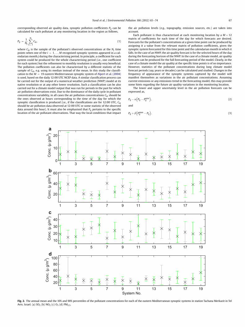
Fig. 2. The annual mean and the 10% and 90% percentiles of the pollutant concentrations forAviv, Israel. (a) SO2 (b) NO2 (c) O3 (d) PM2.5.

the air pollution levels (e.g., topography, emission sources, etc.) are taken intoaccount.

Each pollutant is thus characterised at each monitoring location by a M � 12matrix of coefficients for each time of the day for which forecasts are desired.Forecasts for the pollutant’s concentrations at a given time point can be produced byassigning it a value from the relevant matrix of pollution coefficients, given thesynoptic system forecasted for this time point and the calendarianmonth inwhich itfalls. In the case of an NWP, the air quality forecast is for the selected hours of the dayduring the forecasting horizon of the NWP. In the case of a climate model, air qualityforecasts can be produced for the full forecasting period of the model. Clearly, in thecase of a climate model the air quality at the specific time points is of no importance.However, statistics of the pollutant concentrations during long climate modelforecast periods (say, years or decades) can be calculated and studied. Changes in thefrequency of appearance of the synoptic systems captured by the model willmanifest themselves as variations in the air pollutant concentrations. Assumingcurrent emissions or any emissions trend in the forecasting model, this may providesome hints regarding the future air quality variations in the monitoring location.

The lower and upper uncertainty level in the air pollution forecasts can beexpressed as,

Pij � a�Pij � Pmin

ij

�; (2)

and

Pij þ b�Pmaxij � Pij

�; (3)

11 13 15 17 19

11 13 15 17 19

11 13 15 17 19

11 13 15 17 19tem No.

each of the eastern Mediterranean synoptic systems in station Tachana Merkazit in Tel

Yuval et al. / Environmental Pollution 166 (2012) 65e7468

where Pminij and Pmax

ij are the minimum and maximum of the sample Cik , respec-tively, and a and b are coefficients in the range ½0 1 � that can be selected accordingto the desired confidence level. Alternatively, low and high percentile values of theset Cik can serve as the lower and upper limits of the prediction. The most suitablestatistics to define the system coefficients and their limits may vary betweenpollutants and regions. They can be determined by a cross-validation process inwhich the level of risk is set in advance by the selection of the a and b parameters orthe values of the limiting percentiles. For this study, we used the mean value(defined in Eq. (1)) as a system coefficient, and low and high percentiles foruncertainties. It must be noted that these uncertainty calculations assume an airpollution emission scenario similar to the one during the characterising period. Theunknown future variations in the pollution emissions are not accounted for in thiswork and the possible implications are discussed later.

The process described above of forecasting a pollutant’s concentration and itsuncertainty range, based on the synoptic system classification, can be carried out fora few monitoring stations in a region. This step involves very little additional workand costs, and it results in spatial maps of the forecasted pollution levels and theiruncertainties.

195 200 205 210

740

745

750a

b

195 200 205 210

740

745

750c

d

195 200 205 210

740

745

750

e f

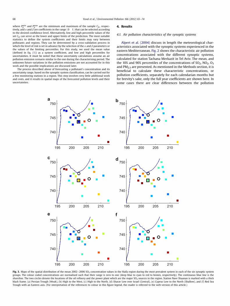
Fig. 3. Maps of the spatial distribution of the mean 2002e2006 SO2 concentration values ingroups. The colour coded concentrations are normalised such that their range is zero to oshoreline. The two circles denote the locations of the oil refinery and the power plant whichblack frame. (a) Persian Trough (Weak), (b) High to the West, (c) High to the North, (d) ShTrough with an Eastern axis. (For interpretation of the references to colour in this figure le

4. Results

4.1. Air pollution characteristics of the synoptic systems

Alpert et al. (2004) discuss in length the meteorological char-acteristics associated with the synoptic systems experienced in theeastern Mediterranean. Fig. 2 shows the characteristic air pollutionconcentrations associated with the different synoptic systems,calculated for station Tachana Merkazit in Tel Aviv. The mean, andthe 10% and 90% percentiles of the concentrations of SO2, NO2, O3and PM2.5 are presented. As mentioned in the Methods section, it isbeneficial to calculate these characteristic concentrations, orpollution coefficients, separately for each calendarian months butfor brevity’s sake, only the full year coefficients are shown here. Insome cases there are clear differences between the pollution

195 200 205 210

740

745

750

195 200 205 210

740

745

750

195 200 205 210

740

745

750

the Haifa region during the most prevalent system in each of the six synoptic systemne (deep blue to cyan to red to brown, respectively). The continuous blue line is theare the major SO2 sources in the region. Station Nave Shaanan is marked with a thick

arav Low over Israel (Central), (e) Cyprus Low to the North (Shallow), and (f) Red Seagend, the reader is referred to the web version of this article.)

Yuval et al. / Environmental Pollution 166 (2012) 65e74 69

coefficients of the different synoptic systems and between thesystem groups. For example, the SO2 concentrations associatedwith systems 1e3, the Red Sea Troughs, are much higher than thoseof systems 4e6 of the Persian Trough group. However, the rangebetween the 10th and 90th percentile values can be very wide andthere is some overlap between the ranges of all four pollutants, foralmost all the systems.

Each synoptic system is associated with a certain typical winddirection that determines the main axis of air pollution dispersionand thus, to a certain extent, its spatial concentration pattern. (Thelevels of the concentrations are mainly determined by the typicalwind speed, atmospheric stratification conditions and the atmo-spheric chemistry rates.) Fig. 3 shows maps of the spatial patternsof the mean SO2 concentrations in the Haifa bay area for a repre-sentative system from each of the six synoptic system groups. Therepresentative systemswere selected as the most prevalent in theircorresponding groups. The only significant SO2 sources in theregion are the oil refinery and the power plant, located at its centre(see Fig. 3). When the region is dominated by the Persian Troughand the High to the West systems, the typical winds are from thenorthwest. As a result, the mean SO2 concentrations during thesesystems (Fig. 3a and b, respectively) are highest southeast of the

December Ja

20

40

60

80a

Con

c. (µ

g/m

3 )

December Ja

102030405060

b

Con

c. (µ

g/m

3 )

December Ja

102030405060

c

Con

c. (µ

g/m

3 )

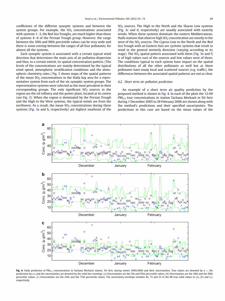
Fig. 4. Daily prediction of PM2.5 concentrations in Tachana Merkazit station, Tel Aviv, dupredictions by a x and the uncertainties are denoted by the solid line envelope. (a) Uncertainpercentile values. (c) Uncertainties are the 25th and the 75th percentile values. The uncerrespectively.

SO2 sources. The High to the North and the Sharav Low systems(Fig. 3c and d, respectively) are usually associated with easterlywinds. When these systems dominate the eastern Mediterranean,Haifa stations that observe high SO2 concentration aremostly to thewest of the SO2 sources. The Cyprus Low to the North and the RedSea Trough with an Eastern Axis are cyclonic systems that result inwind in the general westerly direction (varying according to itsstage). The SO2 spatial pattern associated with them (Fig. 3e and f)is of high values east of the sources and low values west of them.The conditions typical to each system have impact on the spatialdistributions of all the other pollutants as well but as thesepollutants have many local and scattered sources (e.g. traffic), thedifferences between the associated spatial patterns are not as clear.

4.2. Short term air pollution prediction

An example of a short term air quality prediction by theproposed method is shown in Fig. 4. In each of the plots the 12:00PM2.5 true concentrations in station Tachana Merkazit in Tel Avivduring 1 December 2005 to 28 February 2006 are shown alongwiththe method’s predictions and their specified uncertainties. Thepredictions in this case are based on the mean values of the

nuary February

nuary February

nuary February

ring winter 2005/2006 and their uncertainties. True values are denoted by a þ, theties are the 5th and 95th percentile values. (b) Uncertainties are the 10th and the 90thtainty envelope includes 85, 75 and 55 of the 88 true valid values in (a), (b) and (c),

Yuval et al. / Environmental Pollution 166 (2012) 65e7470

concentration samples for each synoptic system (Eq. (1)). Theuncertainty limits shown in Fig. 4a, b and c span the 5e95, 10e90and 25e75 percentiles for each synoptic system, respectively.Naturally, as the uncertainty limits narrow they include less of thereal values within their bounds. Eighty five, 75 and 55 out of the 88valid real data shown in Fig. 4a, b and c, respectively, are within theuncertainty bounds. The large uncertainties shown in Fig. 4 implythat the prediction skills of the proposed method cannot beexpected to be very high. It is important therefore to verify that thepredictions are comparable to those achieved by commonbenchmarks.

0

0.5

1

a

Succ

ess

rate

SynSeaPer

0

0.2

0.4

0.6

0.8b

Succ

ess

rate

0

0.2

0.4

0.6

0.8

c

Succ

ess

rate

0

0.2

0.4

0.6

0.8d

Succ

ess

rate

Monitor

Fig. 5. The success rate at predicting the correct categorical level (Low/Medium/High) of tforecast and persistence with one day lag. The observations are from the stations in the Gus

The two benchmark methods we consider are the seasonal andpersistence forecast methods. The seasonal forecast assigns thepollutant concentration prediction at a certain day to be the meanvalue of the air pollution concentration sample observed at its cal-endarian day during all the years in the study period. Due to therelatively small number of years in the available time series (andthus a small number of time points to calculate each calendarianmean), our calculation included data of the relevant calendarian dayand its adjacent six days (e.g., the calendarianmean of 15 January at12:00 was calculated using the time points on January 12e18 at12:00 in all the years in the study period). A second benchmark,may

optic systemssonalsistence

ing stations

he true daily 12:00 pollution concentration by the synoptic system forecast, seasonalh Dan network during the study period 1995e2006. (a) SO2, (b) NO2, (c) O3, (d) PM2.5.

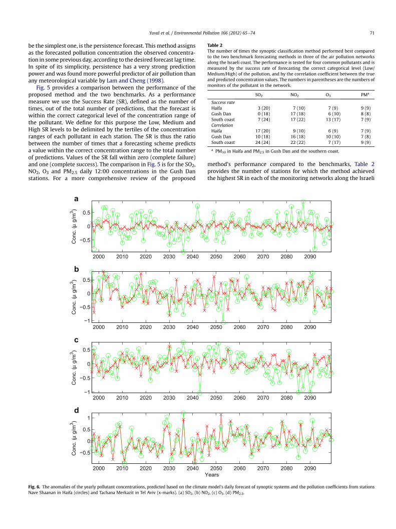
Table 2The number of times the synoptic classification method performed best comparedto the two benchmark forecasting methods in three of the air pollution networksalong the Israeli coast. The performance is tested for four common pollutants and ismeasured by the success rate of forecasting the correct categorical level (Low/Medium/High) of the pollution, and by the correlation coefficient between the trueand predicted concentration values. The numbers in parentheses are the numbers ofmonitors of the pollutant in the network.

SO2 NO2 O3 PMa

Success rateHaifa 3 (20) 7 (10) 7 (9) 9 (9)Gush Dan 0 (18) 17 (18) 6 (10) 8 (8)South coast 7 (24) 17 (22) 13 (17) 7 (9)CorrelationHaifa 17 (20) 9 (10) 6 (9) 7 (9)Gush Dan 10 (18) 16 (18) 10 (10) 7 (8)South coast 24 (24) 22 (22) 7 (17) 9 (9)

a PM10 in Haifa and PM2.5 in Gush Dan and the southern coast.

Yuval et al. / Environmental Pollution 166 (2012) 65e74 71

be the simplest one, is the persistence forecast. This method assignsas the forecasted pollution concentration the observed concentra-tion in some previous day, according to the desired forecast lag time.In spite of its simplicity, persistence has a very strong predictionpower and was found more powerful predictor of air pollution thanany meteorological variable by Lam and Cheng (1998).

Fig. 5 provides a comparison between the performance of theproposed method and the two benchmarks. As a performancemeasure we use the Success Rate (SR), defined as the number oftimes, out of the total number of predictions, that the forecast iswithin the correct categorical level of the concentration range ofthe pollutant. We define for this purpose the Low, Medium andHigh SR levels to be delimited by the tertiles of the concentrationranges of each pollutant in each station. The SR is thus the ratiobetween the number of times that a forecasting scheme predictsa value within the correct concentration range to the total numberof predictions. Values of the SR fall within zero (complete failure)and one (complete success). The comparison in Fig. 5 is for the SO2,NO2, O3 and PM2.5 daily 12:00 concentrations in the Gush Danstations. For a more comprehensive review of the proposed

2000 2010 2020 2030 2040

−0.5

0

0.5

Con

c. (µ

g/m

3 )

a

2000 2010 2020 2030 2040−1

−0.5

0

0.5

Con

c. (µ

g/m

3 )

b

2000 2010 2020 2030 2040−1

−0.5

0

0.5

Con

c. (µ

g/m

3 )

c

2000 2010 2020 2030 2040

−0.5

0

0.5

1

Y

Con

c. (µ

g/m

3 )

d

Fig. 6. The anomalies of the yearly pollutant concentrations, predicted based on the climateNave Shaanan in Haifa (circles) and Tachana Merkazit in Tel Aviv (x-marks). (a) SO2, (b) NO

method’s performance compared to the benchmarks, Table 2provides the number of stations for which the method achievedthe highest SR in each of the monitoring networks along the Israeli

2050 2060 2070 2080 2090

2050 2060 2070 2080 2090

2050 2060 2070 2080 2090

2050 2060 2070 2080 2090ears

model’s daily forecast of synoptic systems and the pollution coefficients from stations2, (c) O3, (d) PM2.5.

Yuval et al. / Environmental Pollution 166 (2012) 65e7472

coast. Table 2 also provides the corresponding number of times thatthe proposed method achieved the highest Pearson correlationcoefficient. Examining Fig. 5 and Table 2, it can be concluded thatthe proposed method have a small, but clear advantage, comparedto the benchmarks, especially in the NO2 and PM2.5 forecasts. It isinteresting to note that the additional information that the synopticsystem forecast provide does result in some advantage compared tothe simpler methods. However, given the additional efforts itrequires, the advantage of the proposedmethod seemsmarginal forthe short term predictions and adopting this method for routine airquality forecasts might not be warranted.

4.3. Application for future climate air quality assessment

Fig. 6 shows the predicted annual mean anomalies (residualsafter subtracting the mean) of concentrations of SO2, NO2, O3 andPM2.5 for the years 1997e2099, based on synoptic system classifi-cation of the ECHAM4/OPYC3 model output and the pollutioncoefficients calculated for stations Nave Shaanan in Haifa andTachanaMerkazit in Tel Aviv. Using anomalies of the concentrationsenables plotting the two forecasts on the same scale (there aresignificant differences in the mean pollution levels between thetwo stations) and better appreciation of the magnitude of the longterm variability. The annual variability is relatively small, with anamplitude of about 1 mg/m3 for all the pollutant series. Theamplitude of the variations in the SO2 in Nave Shaanan is muchlarger than that in Tachana Merkazit. The location of Nave Shaananis very close to the local SO2 sources (see Fig. 3), and being situatedon a mountain slope at the elevation of the stacks leads to largevariations in the SO2 concentrations during different synopticsystems. Commensurate amplitudes of the annual variations in thetwo stations exist for all the other pollutants.

The correlation between the two forecasts are 0.77, 0.44, 0.40and 0.85 for SO2, NO2, O3 and PM2.5, respectively. The PM2.5 levels inIsrael are dominated by transboundary transport of sulphates andnitrates from eastern Europe, and by dust particles from thesurrounding deserts (Erel et al., 2007). The spatial variability ofPM2.5 and the associated variability in the PM2.5 pollution coeffi-cients are thus small and result in similar long term PM2.5 forecastin the two stations. Most of the SO2 in Israel is due to largeindustrial plants, emitting quite constantly 24 h a day. The temporalvariations in the SO2 concentrations are therefore mainly due to thevariability in themeteorological conditions which are characteristicto different synoptic systems. Thus, the correlation between theSO2 forecasts for the two locations is also relatively high. The lowercorrelation between the forecasts of NO2 and O3 is probably due tothe fact that the concentrations of these two pollutants dependmainly on the NOx and VOCs emissions of the local traffic.

2000 2010 2020 2030 2040

−1

0

1

2

Ye

Con

c. (µ

g/m

3 )

Fig. 7. The anomalies of the yearly PM2.5 concentrations, considering only days which weranomalies from the annual means, with the means calculated taking only the concentratiopentagrams denote the mean annual values due to synoptic systems transporting PM2.5 tomark values due to synoptic systems transporting mineral dust from northern Africa (system

Variations in the traffic emissions as a result of changes in the trafficpatterns and volumes, the weekly cycle, due to holidays, etc. areclearly not related to the dominating synoptic system. This resultsin differences between the NO2 and O3 pollution coefficientscalculated for different stations for each synoptic system, and todifferent temporal variability patterns in the long term forecasts.

An example of the possible importance of long term forecasts isgiven in Fig. 7. The figure shows the 1997e2099 anomalies of theyearly PM2.5 concentrations in Haifa, considering only days whichwere assigned synoptic system belonging to one of two specialgroups. One group includes systems 4, 5, 6 and 8, which transportto Israel PM2.5, mainly sulphates and nitrates, from eastern Europe.The second group consists of systems 2, 12, 13, 18 and 19, whichtransport to Israel mineral dust from northern Africa. The shownvalues are the anomalies from the annual means, with the meanscalculated taking only the concentration values during days whenthe mentioned synoptic system groups were present (other daysassigned zero value). No clear trend is noted in the levels of thedust-related PM during the 103 years period. However, the levels ofPM2.5 transported from eastern Europe is increasing with a lineartrend that results in additional 2 mg/m3 during this period. Giventhat eastern Europe transport is a major contributor to the PM2.5burden in Israel (Asaf et al., 2008; Erel et al., 2007), this is animportant and interesting finding, suggesting that local controlmeasures to reduce PM emissionsmay not be sufficient to abate thefuture PM2.5 in Israel.

5. Discussion and conclusions

This study proposes a very simple method for assessing thefuture air quality in a location for which historical air pollutionrecords and a corresponding set of classifications of the weather tosynoptic systems are available. The method was shown to becomparable, and slightly better than the seasonal and one-day-lagpersistence forecasts in a three air pollution networks along theIsraeli Mediterranean coast. By its nature, persistence cannot beused for long term air quality forecasts and seasonal forecasting isnot useful for studies which consider possible climatologicalchanges. Given an output of a climate model for the region, themethod proposed by this work enables studying future air quality ina changing climate scenario. The climate change effect is incorpo-rated in the variations in the frequency of the appearance of thevarious synoptic patterns. This assessment can serve as an alter-native to the more complicated and expensive approach of usingchemical transport air pollution schemes driven by climate models(Jacob and Winner, 2009). However, a major drawback of theproposed approach is its use of constant pollutant coefficients.Moreover, the accuracy of our assessment depends to a large degree

2050 2060 2070 2080 2090ars

e assigned synoptic system belonging to one of two groups. The shown values are then values during days when the mentioned synoptic systems groups were present. Thethe eastern Mediterranean from eastern Europe (systems 4, 5, 6 and 8). The diamondss 2, 12, 13, 18 and 19). The solid lines are linear regression lines fitted to the two curves.

1998 2000 2002 2004 2006

5

6

7

8

9

10

11

12

Con

c. (µ

g/m

3 )

a

1998 2000 2002 2004 2006

20

25

30

35

Con

c. (µ

g/m

3 )

b

1998 2000 2002 2004 2006

50

55

60

65

70

75

Con

c. (µ

g/m

3 )

c

1998 2000 2002 2004 2006

20

21

22

23

Con

c. (µ

g/m

3 )

d

Fig. 8. The real 1997e2006 annual mean pollution concentrations in Haifa, Israel (circles) and the corresponding hindcasting estimates (x-marks) by the synoptic classificationmethod. (a) SO2, (b) NO2, (c) O3, (d) PM2.5.

Yuval et al. / Environmental Pollution 166 (2012) 65e74 73

on the ability of the climate model to produce synoptic systemssimilar to the real ones, and with frequencies which are similar tothe observed ones.

The accuracy of the proposed method is a concern in its appli-cation for forecasting long term trends in the air quality. However,a much larger concern is the caveat hidden in the assumption ofcurrent air pollution emission levels while calculating the pollutioncoefficients. The last few decades have seen variations in airpollution emissions in the developed world (happily, mainlydecreasing trends) whose impact on the air quality probably dwarfsthe possible variations due to different prevalence of the synopticsystems in the future. For example, SO2 levels in Haifa, Israel, werereduced by more than an order of magnitude in the last 20 yearsand are expected to drop to almost zero level once the local powerplant and refineries switchover from use of fuel oil to natural gas.VOC levels in most developed countries experienced a similar drop(Dollard et al., 2007) and will probably be further reduced with theon-going improvements in private vehicle emission controls. Theintroduction of electric cars will bring about a decrease in bothVOCs and NOx emissions and thus also in the O3 levels. Theincreased use of non-combustive energy production sources andbetter emission controls on industrial plants will result ina decrease in PM, NOx and O3.

Fig. 8 shows a comparison between the real annual average1997e2006 concentrations of SO2, NO2, O3 and PM2.5 in NaveShaanan, Haifa, and the hindcasting by the proposed method. Thesynoptic system pollution coefficients were calculated using thedata during the whole observation period and are thus providinginformation on that period’s mean levels. This results in hindcastsfor these pollutantswhich are almost nonvariant in time, in contrast

to the very significant trends in the local SO2, NO2 and O3 levels. Thesources of PM2.5 in Haifa, much of it desert dust and transportedsulphates and nitrates from eastern Europe, have not significantlychanged during 1997e2006. However, even for this pollutant thehindcast is not close to the real record, probably due to insufficientaccuracy in capturing the yearly variations in the synoptic systemoccurrence by the climate model. Cheng et al. (2007b) assumedthree different scenarios of air pollution emissions in their assess-ment of climatic impact on air quality however, there is no guar-antee that any of these scenarios will materialise. Future airpollutants emissions are an unknown but given the examplesshown in Fig. 8, it is very probable that their variations will havea larger impact on future air pollution levels compared to the rela-tively small variations expected due to any reasonable variations inthe occurrence of synoptic systems in a changing world climate.

Acknowledgements

This work was supported by the Technion Center for Excellencein the Exposure Science and Environmental Health. The authorswould like to thank the anonymous reviewers for their help whichresulted in a more focused and streamlined manuscript.

References

Alpert, P., Ostinski, I., Ziv, B., Shafir, H., 2004. Semi-objective classification for dailysynoptic systems: application to the eastern Mediterranean climate change.International Journal of Climatology 24, 1001e1011.

Asaf, D., Pedersen, D., Peleg, M., Matveev, V., Luria, M., 2008. Evaluation of back-ground levels of air pollutants over Israel. Atmospheric Environment 42,8453e8463.

Yuval et al. / Environmental Pollution 166 (2012) 65e7474

Carmichael, G.R., Sandu, A., Chai, T., Daescu, D.N., Constantinescu, E.M., Tang, Y.,2008. Predicting air quality: improvements through advanced method tointegrate models and measurements. Journal of Computational Physics 227,3540e3571.

Chen, Z.H., Cheng, S.Y., Li, J.B., Gou, X.R., Wang, W.H., Chen, D.S., 2008. Relationshipbetween atmospheric pollution processes and synoptic pressure patterns innorthern China. Atmospheric Environment 42, 6078e6087.

Cheng, C.S., Campbell, M., Li, Q., Li, G., Auld, H., Day, N., Pengelly, D., Gingrich, S.,Yap, D., 2007a. A synoptic climatological Approach to assess climatic impact onair quality in southecentral Canada. Part I: historical analysis. Water, Air andSoil Pollution 182, 131e148.

Cheng, C.S., Campbell, M., Li, Q., Li, G., Auld, H., Day, N., Pengelly, D., Gingrich, S.,Yap, D., 2007b. A synoptic climatological Approach to assess climatic impact onair quality in southecentral Canada. Part II: future estimates. Water, Air and SoilPollution 182, 117e130.

Chou, C.J., Neelin, D., Tu, J.Y., Chen, C.T., 2006. Regional tropical precipitation changemechanisms in ECHAM4/OPYC3 under global warming. Journal of Climate 19,4207e4223.

Dollard, G.J., Dumitrean, P., Telling, S., Dixon, J., Derwent, R.G., 2007. Observed trendsin ambient concentrations of C2eC8 hydrocarbons in the United Kingdom overthe period from 1993 to 2004. Atmospheric Environment 41, 2559e2569.

Erel, Y., Kalderon-Asael, B., Dayan, U., Sandler, A., 2007. European atmosphericpollution imported by cold air masses to the Eastern Mediterranean during thesummer. Environmental Science and Technology 41, 5198e5203.

Ganor, E., Osetinski, I., Stupp, A., Alpert, P., 2010. Increasing trend of African dust,over 49 years, in the eastern Mediterranean. Journal of Geophysical Research115, D07201. doi:10.1029/2009jD012500.

IPCC, 2007. Climate change 2007: the physical sciences basis. In: Solomon, S.,Qin, D., Manning, M., Chen, Z., Marquis, M., Averyt, K.B., Tignor, M., Miller, H.L.

(Eds.), Contribution of Working Group I to the Fourth Assessment Report of theIntergovernmental Panel on Climate Change. Cambridge University Press,Cambridge, UK and New York, USA.

Jacob, D.J., Winner, D.A., 2009. Effects of climate change on air quality. AtmosphericEnvironment 43, 51e63.

Lam, K.C., Cheng, S., 1998. A synoptic climatological approach to forecast concen-trations of sulfur dioxide and nitrogen oxides in Hong Kong. EnvironmentalPollution 101, 183e191.

Pearce, J.L., Beringer, J., Nicholls, N., Hyndman, R.J., Petteri, U., Tapper, N.J., 2011.Investigating the Influence of Synoptic-scale Meteorology on Air Quality UsingSelf-organizing and Generalizing Additive Modelling.

Pope III, C.A., Bates, D.V., Raizenne, M.E., 1995. Health effects of particulate air pollution:time for reassessment? Environmental Health Perspectives 103, 472e480.

Roeckner, E., Coauthors, 1996. The Atmospheric General Circulation Model ECHAM-4: Model Description and Simulation of Present-day Climate. Max-Planck-Institute für Meteorologie. Rep. 218, 90pp.

Schwartz, J., Dockery, D.W., 1992. Increased mortality in Philadelphia associatedwith daily air pollution concentrations. The American Review of RespiratoryDisease 145, 600e604.

Seinfeld, J.H., Pandis, S.N., 1998. Atmospheric Chemistry and Physics, from AirPollution to Climate Change. Wiley, New York.

Tanner, P.A., Law, P., 2002. Effects of synoptic weather systems upon the air qualityin an Asian megacity. Water, Air and Soil Pollution 136, 105e124.

Triantafyllou, A.G., 2001. PM10 pollution episodes as a function of synoptic clima-tology in a mountainous industrial area. Environmental Pollution 112, 491e500.

Vallero, D., 2007. Fundamentals of Air Pollution, fourth ed. Academic Press, NewYork.World Health Organization, 2006. Air Quality Guidelines for Particulate Matter,

Ozone, Nitrogen Dioxide and Sulfur Dioxide. Global Update 2005. WHO Press,Geneva.