exploring for the determinants of credit risk in credit

Exploring for the Determinants of Credit Risk inCredit Default Swap Transaction Data.

Didier Cossin∗ & Tomas Hricko∗∗

October 2001

Comments Welcome

∗HEC, University of Lausanne, CH-1015 Lausanne, SwitzerlandTel: 41 21 692 34 69Fax: 41 21 692 33 05Email: [email protected]∗∗Email: [email protected]

Acknowledgments:We thank Fabio Alessandrini, Jerome Detemple, Paul Ehling, Hans-Ulrich

Gerber, Sarkis J. Khoury, David Mayers, Hugues Pirotte, Waymond Rodgers,Frank Skinner, René Stulz and Heinz Zimmermann and participants at theEFMA and IAFE meetings for their help and comments. Financing wasprovided by the Swiss National Science Foundation (FNRS).

1

Exploring for the Determinants of Credit Risk inCredit Default Swap Transaction Data.

October 2001

Comments Welcome

2

Abstract

We investigate the influence of various fundamental variables on a cross-section of credit default swap rates. Credit default swap rates can be seenas an alternative proxy for credit risk. Therefore our findings are relevantnot only for the understanding of credit default swaps but for credit risk ingeneral. The fundamental variables include ratings, interest rate data andstock market related information such as variance and leverage (so called ”structural variables ”). We test for the stability of the influence of the dif-ferent fundamental variables along several lines. We find evidence that mostof the variables predicted by credit risk pricing theories have a significantimpact on the observed levels of credit default prices. We also provide aninternational analysis of corporate credit risk, as half of our corporate sampleis not US based, as well as some results on sovereign credit risk. Using thisinformation we are able to explain a significant portion of the cross-sectionalvariation in our sample with adjusted R2 reaching 82% using the variablespredicted by classical theoretical models. However there are important be-havioral differences between high rated and low rated underlyings, sovereignand corporate underlyings and underlyings from different markets (US vs noUS), differences that we examine. In particular, we provide evidence thatratings, while having strong explanatory power overall in cross-section, havestrong non-linearities, threshold effects with US corporates (i.e. have signif-icantly different impact on high rated and low rated companies) while theytend to behave consistently with sovereigns. We also show that the expectednegative relationship of credit risk to interest rates is valid for low credit risklevel but not for high credit risk levels. Also, while US interest rate levelsseem to matter for credit risk worldwide, the local slope of the yield curvematters more than the US’. Structural variables (volatility, leverage) have

3

strong explanatory power for high and low rated corporates and drive mostof the credit risk when ratings have little explanatory power (eg, when creditrisk is low in US corporates). In general, structural variables provide com-plementary information to ratings (ie, are not subsumed in ratings), and canbe seen as the primary source of information on credit risk in some subsam-ples (high rated US). The past evolution of stock prices remains significantas well beyond leverage changes, pointing out possibly to behavioral financeissues in the credit risk markets. Finally, contrarily to expectations, prelim-inary results tend to show that liquidity does not seem to play a large rolein this OTC exotic market.

4

1 Introduction

Credit risk has received much attention in the academic literature. The bulkof the work has focused on theoretical valuation issues. There is far lessresearch on the empirical side. Nearly all of the empirical work investigat-ing credit risk has focused on the bond market. The main approach was toexplain the determinants and the dynamics of the credit spread, hence thedifference between the yield on a bond of a risky counterparty and a gov-ernment bond. Government and corporate bonds differ in a variety of ways,which makes the credit spread an imperfect proxy for credit risk. Some ofthe issues are addressed in Duffee (1998). Financial innovation has led tothe emergence of a new kind of derivative written directly on a credit risk,credit derivatives. The Credit Default Swap (CDS) is the most used CreditDerivative. A Credit Default Swap is an instrument that provides its buyerwith a lump sum payment made by the seller in the case of default (or other” credit event ”) of an underlying reference entity against the periodic pay-ment made by the buyer. This periodic payment expressed as a functionof its notional value is the CDS rate. No academic study that we know ofhas investigated the empirical behavior of credit default swap rates. Such astudy has strong implications for our understanding of credit risk behavior.It represents an opportunity to study credit risk from another instrumentthan the fixed income instruments (bonds, swaps) analyzed previously.We test for the influence of the theoretical factors predicted by the re-

duced and the structural form literature. Moreover, we test for the stabilityof the influences by using a cross-section of credit default swap rates on avariety of underlyings.Our study differs from all existing studies done on factors influencing

credit risk in some respect. Credit derivatives have been around for someyears but they have only in the recent past begun to be used widely in themarket. Credit default swaps are supposed to allow the transfer of pure creditrisk from one counterparty to another. They can be designed to provideprotection against consequences of default in a variety of ways. In the purestform they provide a pre-specified payment in the event of default. If this isa fixed payment then the value of the credit default swap is only influencedby the occurrence of default. The payment can be specified in terms of anotherwise risk free bond, which makes it dependent on the term structure of

5

interest rates. In this case the following relationship has to hold

Credit risky bond+ Credit default swap = Riskfree bond

Due to this fundamental relationship we can use the prices of credit de-fault swaps, respectively their swap rate, in order to analyze indirectly thefactors influencing the credit risk of the underlying parties of the credit de-fault swaps. This approach has many advantages. It is not subject to someof the flaws of previous studies investigating credit risk as measured by thespread of the risky bond yield relative to the risk free rate. As the contractsare written directly on a credit event they are not subject to the distortionof call features and other covenants. Furthermore, credit default swaps arenot interest rate based instruments (while other credit risk instruments suchas bonds and swaps are). They allow for a direct analysis of credit risk (andthe influence of interest rates thereupon), rather than for an indirect analysisof credit risk as embedded in an interest-rate based security. Finally, theypresent a somewhat standardized instrument to study and compare creditrisk in different countries, as well as credit risk coming from corporates ver-sus sovereigns. However they are also subject to some disadvantages whichare linked to their nature as OTC contracts. The main disadvantage is theirlack of liquidity and of a secondary market. We only observe the prices atinitiation of the contract. Secondary trading or a closing of the position isdone directly in-between the counterparties or with another broker. More-over some of the refinements of the contract like exact specification of thepayment in case of default as well as the exact definition of default can anddo vary slightly from contract to contract.We proceed with a brief literature review of empirical studies of credit

risk before addressing how classical theoretical models would price creditdefault swaps. We then describe our data and the variables we consideredbased on the theoretical and empirical literature. The empirical investigationthat follows provides results on the impact of these variables as well as oninternational differences and other underlying differences.

6

2 Literature review

The literature on such a recent instrument as the Credit Default Swap isby necessity scarce. Nonetheless, several papers have addressed the the-oretical pricing of credit derivatives during the last few years. Longstaffand Schwartz (1995) present the pricing of credit spread options based onan exogenous mean-reverting process for credit spreads. Das (1995) uses astructural-form compound option model to price credit derivatives in a sto-chastic interest environment. The structure used corresponds more to creditspread options though than to credit default swaps. Duffie (1999) presents asimple argumentation for the replication of Credit Default Swaps as well asa simple reduced form model of the instrument. Das and Sundaram (2000)use a Heath-Jarrow-Morton framework to modelize credit spreads directlyand thus generate a flexible pricing model that can be used for fitting.Hull andWhite (2000 a and b) develop a reduced-form type pricing model,

with an extension to several underlyings and non perfectly correlated default.They calibrate their model based on the traded bonds of the underlying ona time series of credit default swap prices on one underlying.While the literature on Credit Default Swaps is scarce and no complete

empirical analysis has been produced yet that we know of, there is a moresignificant empirical literature on credit risk in general.Some papers have concentrated on a direct analysis of credit ratings as

provided by the big rating agencies. These ratings are important as theyare used extensively in practice as a proxy for credit risk. Some theoreticalmodels also rely on ratings and rating transitions like Jarrow et alii (1997).Moon and Stotsky (1993)\ evaluate the determinants of ratings by each ratingagency in a systematic econometric analysis. Hite and Warga (1997) analyzechanges in ratings during the life of a bond and find some information contentfor down grades at announcement, and little or none for upgrades. Theearlier studies by Katz (1974), Hettenhouse and Sartoris (1976), Weinstein(1977) and Pinches and Singleton (1978) all concluded that there is a lagbetween the arrival of new information and rating changes. Hence ratingsdo not necessarily provide much new information, except for small not veryfrequently traded firms. Further evidence on the changing of ratings throughtime is provided by Lucas and Lonski (1993). They find a trend towards lowerrate debt issues combined with a higher rating volatility in the bond marketduring 1970-1990. Some more evidence on the quality of ratings is provided

7

by Cantor et al. (1997) by analyzing the influence of split rating on pricing.Finally Nickel et al. (2000) analyze the stability of rating transitions. Thework of Altman and Kishore (1996a) and Izvorski (1997) provide some moreevidence on default and recovery rates. Altman and Kishore (1996a) findthat history of default and the resulting default rates are sensitive to somespecific issues and that ratings have no explanatory power on recovery ratesonce seniority is taken into account. Izvorski (1997) concludes that maturity,seniority and the state of the economy are the main determinants of thevalue of firm specific contracts. The influence of maturity is a debated issueas there is no general consensus among the different modelling approacheson its influence on credit risk pricing particularly for below investment gradeissues.

There are only a few studies investigating the determinants of creditspreads. Duffee (1998) finds that the credit spread is negatively relatedto the level of interest rates and the term spread. He also finds that thesensitivity to changes in the term structure is more pronounced for lowerrated bonds. He observes further that changes in bond values might be dueto the influence of the call feature present in a bond. Allessandrini (1998)confirms these findings and concludes further that the business cycle effectis mainly captured by the changes in long-term interest rates. The study byFriedson and Garman (1998) differs from the previous by using new issuesof high-yield bonds to analyze the factors that influence the pricing. Theyfind that changes in the risk free rate, credit spreads and the slope of theyield curve influence the pricing. The more recent study by Collin-Dufresneet al. (1999) uses time series of quoted bond prices to analyze the influenceof various financial variables that should in theory influence changes in yieldspreads. They find that these variables have only limited explanatory power.Moreover the residuals of the regressions are highly cross-correlated pointingto the influence of an unobserved common factor. Some further evidence forco-movements of credit spreads is provided by Batten et al. (1999) in theirstudy on Australian Eurobonds.Some studies have analyzed credit risk from other instruments, notably

on Swaps like Sun and Sundaresan (1993) on Swap quotes and Cossin andPirotte (1997) on swap transaction data. Their results tend to be less ad-vanced on credit risk issues than the previously quoted studies on bondspreads.

8

There is a different group of studies that focus on sovereign debt. Analo-gous to the literature on corporate ratings, sovereign ratings were subject toclose examination. Cantor and Packer (1996) find that the public informationis contained in ratings and that rating changes do have a significant effecton the prices of outstanding debt. Classens and Penacchi (1996) construct amodel that takes into account a number of issuer specific factors. They cal-ibrate their model to the observed prices of Mexican Brady bonds. Kaminand Kleist (1999) analyze the determinants and the evolution of emergingmarket spreads during the 1990s. They find a strong relationship of creditratings, maturity and currency denomination with emerging market instru-ments spreads. They also find evidence for a changing risk premium duringthe time span under consideration. Cumby and Evans (1997) and Dungeyet al. (1999) consider credit quality to be some unobservable random vari-able. Dungey et al. (1999) provide a decomposition of international spreadchanges in a Kalman filter framework. Their main result is that for theCommonwealth countries the first of their three factors (the common factor)displays long-swings that explains most of the changes in credit spreads. Forother countries some country specific influences seem to be more important.A significant improvement within those studies is presented by Eichengreenand Mody (1998). They consider the determinants of emerging market debtvalues by taking into account a possible selectivity bias as some low ratedcountries might have been unable to issues bonds following the emergingmarket turbulences. Their findings confirm that higher quality translatesinto a higher probability of issue and a lower spread. However fundamen-tal information can only explain a fraction of the overall variation in theirsample.

There has not been any advanced study we are aware of that bear onCredit Risk as reflected in Credit Derivatives. We next analyze how differ-ent models would price Credit Default Swaps in order to understand whatvariables are important to consider in our empirical analysis and how thosevariables will affect Credit Default Swap rates. We will not fit a specificmodel to our data here (as this goes beyond the scope of this paper) butrather uncover stylized facts about different variables in order to make ourempirical analysis more clear and pertinent.

9

3 The factors influencing credit risk

3.1 The pricing of a credit default swap

In this section we want to derive the general structure of the pricing of a creditdefault swap and illustrate the differences in pricing among various possibletheoretical approaches. Two strands dominate the theoretical literature oncredit risk today: the structural and the reduced form ones. We will workout the explicit pricing for a structural form model and for a reduced formmodel in order to show the influence of the various parameters analyzed inthe subsequent sections. The pricing is done from the buyers point of view.The buyer will have to make periodic payments as long as there is no defaultof the underlying party. On the other hand he will receive some paymentin the case of default. This payment can be specified in a variety of ways.The payment could be defined as a fixed amount in the simplest case. It canbe the difference between the pre-default value and the recovery value of abond. The most common definition is to define it as the difference betweenthe face value of the bond and the recovery value after default. The payoutis sometimes corrected for accrued interest and implied interest payments.The value of a default swap to the buyer of protection is thus given by

V alue of a credit default swap =

IE0[−NXi=1

exp

µ−Z ti

0

r (u) du

¶· Pr ob (no default until time ti) · Swap rate

·Notional + expµ−Z τ

0

r (u) du

¶Pr ob (default · at · time · τ) · Payment]

(1)

where i is the index of the payments, N is the number of payments untilmaturity and r(u) is the interest rate. The expectations operator in the aboveequation is needed as the interest rate could be stochastic and correlated withthe variables influencing the probability of default.Various models will differon how they determine the probabilities and the payment at default.

10

3.2 A simple structural analysis of Credit Default Swaps

In a first step we will develope the pricing for a structural model, with nonstochastic interest rates. It is clear that this model is only applicable directlyfor corporate underlyings. Some evolution of the model could be used forsovereigns in the spirit of Classens and Penacchi (1996). Following the basicMerton (1974) framework we assume that the firm value V follows a geometricBrownian motion given by

dV/V = (r − d) · dt+ σv · dz (2)

where r is the instantaneous risk-free rate, d is the continuous dividendyield and σv is the volatility of the firm value process. The firm will defaultif this value breaches some pre-specified default level denoted H. We willassume that this default level is an exogenously fixed constant. It could bea deterministic function of time. Black and Cox (1977) use a deterministicexponential barrier to model the effect of bond indenture provisions on thevalue of risky debt. We could use a similar functional form to model thedefault boundary. Another possible extension would be in the spirit of Leland(1994) and Leland and Toft(1996). In their model the default boundaryis determined endogenously by maximizing the value of equity respectivelyto the value of the firm. For simplicity we maintain the assumption of afixed constant default boundary. The value of the credit default swap iscomparable to the sum of a number of barrier options on the firm value.The methodology and notation we use for the pricing of the barrier optionsfollows the work of Rich (1994). The probability of no default until time i isobtained as

Pr ob (no default until time i) (3)

= Pr ob (VTi > H, inf Vt > H)

= Pr ob (VTi > H)− Pr ob (VTi > H, inf Vt < H)= N

µ−H/V0 + µ · (ti)σ ·√ti

¶− exp

µ2 ·H/V0 · µ

σ2

¶N

µ−H/V0 − µ · tiσ ·√ti

¶where :

Vt = firm value process

H = default boundary (possibly the face value of debt)

µ = r − d− σ2

2for all t from 0 to Ti

11

With these probabilities we can price one leg of the credit default swap.The value of the periodic payments is obtained as

Part1 = Swap rate ·Notional ·NXi=1

N

µ−H/V0 + µ · (ti)σ ·√ti

¶− exp

µ2 ·H/V0 · µ

σ2

¶N

µ−H/V0 − µ · tiσ ·√ti

¶(4)

Now we proceed to the pricing of the second leg of the default swap, whichis the payment in the case of default. We assume that the recovery value isjust a discount on the face value. This is not an unreasonable assumptionif the recovery rate can be estimated ex-ante with some degree of certainty.We could make the recovery rate a function of time. The valuation couldalways be done by solving numerically the integral given in equation number1. On the other hand the recovery rate could be a function of the value ofthe assets at time of default. However this value is known to us as default istriggered when the firm value crosses the level H as long as default occurs atany time before maturity. Therefore the assumption that the recovery rateis a function of the asset value at the time of default, would just make itdependent on H contrarily to Merton (1974) where a European type settingis used. If the underlying firm value process is a jump-diffusion process, themodelling of a recovery rate that depends on the asset values of the firm atdefault would be more complicated. Under the above assumptions the valueof the second part is given by

Part2 = IE0 [exp (−r · τ) Pr ob (default · at · time · τ) · Payment]=

Z T

0

Payment (H, τ) · exp (−r · τ) · h (τ) dτwhere :

h (τ) = first passage time density of the process v at the level H

h (τ) =− ln

³HV0

´σ√τ 3

n¡x− σ

√τ¢

x =ln¡V0H

¢+ (µ+ σ2) τ

σ√τ

(5)

Under the assumption that the recovery rate is a function of H or the face

12

value we can simplify the above integral to

Part2 = Payment ·³(H/V0)

a+m ·N (w) + (H/V0)a−mN³w − 2mσ

√T´´

where :

a =µ

σ2

m =

pµ2 + 2 · ln (r) · σ2

σ2

w =ln³HV0

´+m · σ2 · T

σ ·√T (6)

The valuation equation would be more complicated if the interest ratewere considered stochastic and correlated with the firm value process. Wemight not be able to obtain a closed form solution for this case dependingon the choice of the process for the stochastic interest rate.Because the value of the firm follows a diffusion process the probability of

default goes to zero as the maturity of the contract goes to zero. Thereforethe credit spread on a risky bond implied by such a model goes to zero aswell. Empirically however default spreads do not go to zero with decreasingmaturity but they remain positive. One possibility to take into account thatfirm value can drop suddenly is to model the firm value process as a jump-diffusion process. Zhou (1997) follows this path and obtains a closed formsolution for the value of a bond under some restrictions and proposes the useof the Monte Carlo methodology for the valuation in the general case.The factors that influence the value of the credit default swap in a classical

structural model such as the one proposed here are the distance from thedefault boundary, the value of the assets of the company, the volatility of thevalue of the company, the level of the interest rate and the time to maturityof the credit default swap. In the earliest structural model, the Mertonmodel, it was assumed, that the default boundary was just the face valueof debt. In the later models the default boundary was given exogenouslyor determined endogenously as in Leland(1994), Leland and Toft (1996) andAnderson and Sundaresan (1996). Even if we don’t observe the exact value ofthis boundary we can identify the influence of various factors on the distancefrom this boundary. A decrease in the stock price will lower the distanceto this boundary, the same is true for an increase in leverage. An increasein volatility would also increase the probability of default as the likelihoodincreases that the firm value process crosses the default boundary.

13

3.3 A Reduced Form Approach and Implications

We turn now to a reduced form approach. In the reduced form approachthe probability of default is governed by the hazard rate. This is common toall the models like Jarrow and Turnbull (1995), Duffie and Singleton (1997)and Lando (1994/97). The hazard rate denoted h(t) could be a function ofa various other variables.Lando (1994/97) derives some simple representations for the valuation

of credit derivatives. The value of a contingent claim that pays some fixedamount if default has not occurred before that time is obtained as

IEQt

·exp

µ−Z T

t

r (s) ds

¶X · 1I (Γ > T )

¸= (7)

1I (Γ > t) IEQt

·exp

µ−Z T

t

r (s) + λ (s) ds

¶X

¸where Γ is the time of default and λ is the intensity of the Poisson process

governing the default probability. This expression is exactly the value of oneof the payments of the credit default swap rate times the notional conditionalon no default up to that point. The other leg of the default swap would bevalued with the expression for a credit derivative that pays off Z(Γ) if theunderlying defaults at time Γ and zero otherwise. This expression is givenby

IEQt

·exp

µ−Z Γ

t

r (s) ds

¶Z (Γ)

¸= (8)

1I (Γ > t) IEQt

·Z T

t

Z (s) · λ (s) expµ−Z s

t

r (u) + λ (u) du

¶ds

¸where Γ = is the time of default

The payment Z(s) would in our case be defined as

Z (s) = FV −Re covery valuewhere FV = face value

The recovery value can be defined in a variety of ways. Jarrow andTurnbull (1995) define it as an ex-ante known value. Another possibility is totreat it as being dependent on a number of state variables. Das and Tufano(1996) for instance assume, that the recovery rate is correlated with the

14

default free spot rate. Duffie and Singleton (1998) specify the recovery valueas a fraction of the pre-default value of the bond (Recovery of Market Value).This solution has some advantages on the modelling side while recovery ofFace Value (where the creditor receives a fraction of the promised face value)or Recovery of Treasury (where the creditor receives a fraction of an identicalbut default free bond) are more common (see Jarrow and Turnbull (1995)).A variety of authors have suggested that the default rate could depend

on some state variables reflecting the economic environment and some firmspecific information. Lando (1994/1997) assumes that the hazard rate de-pends on a number of state variables. Jarrow and Turnbull (2000) use thesame kind of process and assume that the hazard rate is a function of therandom elements in the evolution of a stock price index and the short terminterest rate. Their hazard rate function is given by

λ (t) = a0 (t) + a1r (t) + βσ1W1 (t) (9)

where a0,a,and β are constants; r is the risk free rate and W1 is a Brown-ian motion governing the unexpected part of the returns of a stock priceindex. Their model can be calibrated to fit some observed structure of de-fault spreads. The constant in their model could depend as well on someparameters related to the firm value like the rating, the leverage or the stockprice volatility. In the reduced form framework the valuation formula wouldbe given by

V alue of a credit default swap = (10)

1I (Γ > t) ·NXi=1

IEQt

·exp

µ−Z Ti

t

r (s) + λ (s) ds

¶X

¸+1I (Γ > t) · IEQt

·Z T

t

Z (s) · λ (s) expµ−Z s

t

r (u) + λ (u) du

¶ds

¸The reduced and the structural form approaches differ significantly in the

way they model the default probabilities. On the other hand the economicaldifferences become much smaller if we use a structural model with a jump-diffusion process for the firm value, thus allowing for sudden drops in thevalue of the firms assets, or if we introduce a hazard rate that depends oneconomic and firm specific factors. Therefore the factors influencing theprices of default swaps are basically the same, but the weighting of theirinfluence is different. The form of their influence on credit risk itself will

15

obviously differ amongst the different modelizations. Based on these modelswe identify a number of factors that should affect the prices of credit defaultswaps and credit risk in general. These factors are primarily in the case ofreduced form models the default process, the interest rate and the recoveryrule as well as the maturity of the instrument.

16

4 The Credit Default Swap Data

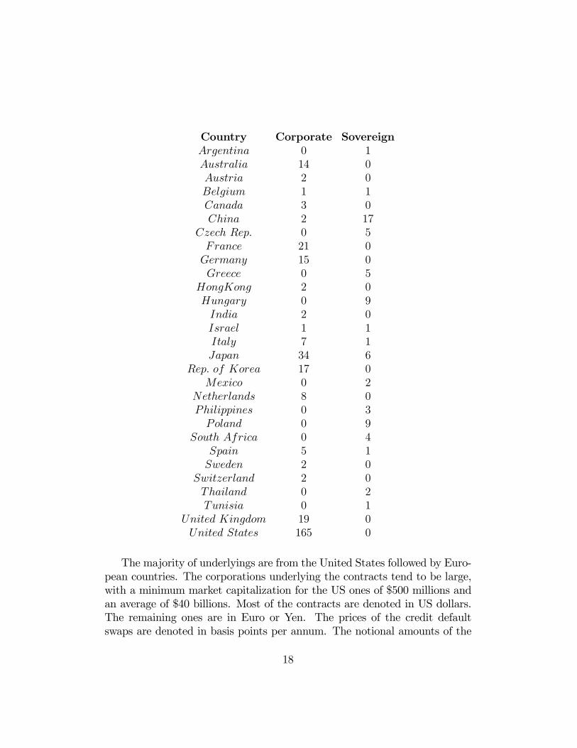
The credit default swap data is obtained from a major London interdealerbroker. The data consist of several thousand one way quotes and 393 realizedtrades. In this study we focus on the realized trades. A one way quote inan OTC market is just the request to sell or to buy a specific instrument forsome specific price. It is not cleared market data with a well defined bid askspread. The traded data on the other hand is market cleared data, hence itrepresents the market consensus on the fair value of the credit default swap attransaction time. Therefore we will restrict ourselves to the 393 observationsof traded contracts. These trades took place during the period from January1998 to February 2000, with observations of all qualities well-spread overthe period (with a peak end of 1998 and beginning of 1999). In the samplewe have 70 sovereign and 323 corporate underlyings. The underlyings comefrom a variety of countries. The domiciles of the underlyings are:

17

Country Corporate SovereignArgentina 0 1Australia 14 0Austria 2 0Belgium 1 1Canada 3 0China 2 17

Czech Rep. 0 5France 21 0Germany 15 0Greece 0 5

HongKong 2 0Hungary 0 9India 2 0Israel 1 1Italy 7 1Japan 34 6

Rep. of Korea 17 0Mexico 0 2

Netherlands 8 0Philippines 0 3Poland 0 9

South Africa 0 4Spain 5 1Sweden 2 0

Switzerland 2 0Thailand 0 2Tunisia 0 1

United Kingdom 19 0United States 165 0

The majority of underlyings are from the United States followed by Euro-pean countries. The corporations underlying the contracts tend to be large,with a minimum market capitalization for the US ones of $500 millions andan average of $40 billions. Most of the contracts are denoted in US dollars.The remaining ones are in Euro or Yen. The prices of the credit defaultswaps are denoted in basis points per annum. The notional amounts of the

18

contracts range from 1 to 20 million US$ . The payment at default is definedas the difference between the notional of the credit default swap and therecovery value of a bond on this underlying with the same notional. Devia-tions from the general structure outlined above are possible. For some of thecontracts more detailed procedures in case of default are specified directlybetween the counterparties without the involvement of the broker. Thesecould include for instance the payment of the value of the bond during sometime before the default and other refinements. We have excluded the highestobservation because we consider it to be an outlier. The observation is aquote from a credit default swap of Russia. We realize that the overall valueis instructive, but we believe that as it is the only value of this magnitude itwould bias more our results than add any quantitatively reliable information.The following table summarizes the basic statistics of the data.

Whole US Non USSample Corporate Corporate Corporate Sovereign

Observations 392 323 166 157 69Mean 0.0088 0.0073 0.0054 0.0092 0.0157Median 0.0047 0.0042 0.0034 0.0048 0.0081

Maximum 0.0780 0.0780 0.0335 0.0780 0.0700Minimum 0.0005 0.0011 0.0011 0.0011 0.0005Std. Dev. 0.0119 0.0103 0.0060 0.0132 0.0159Skewness 2.988 3.853 2.993 3.162 1.422Kurtosis 13.171 20.873 12.105 13.782 4.535

RatingsAverage 6.83 6.58 6.47 6.72 7.90

Max 16 16 16 16 12Min 1 1 1 2 1

Table 1: Descriptiv statistics of the credit default swap rates of the wholesample and all the sub-samples.

19

5 The determinants of credit risk: Variableswe consider and our sources

In this section we outline the factors to be analyzed in the subsequent econo-metric analysis. As shown earlier, the choice of those factors is justified bythe existing theoretical literature on the pricing of credit sensitive contracts.Overall, structural models stress the influence of the value of the assets of thecompany, its volatility, the distance from the default boundary (as influencednotably by the leverage), the level of interest rate and the maturity. Reducedform models use also the latter two but exogeneize the default process andthe recovery rule.

1. Credit ratings

Credit ratings are the most widely observed measure of credit quality ofa specific debt issue or the issuing entity in general and remain the mostcommonly used information for the default process and the hazard rate λ.All the reduced form models rely in one way or another on the estimationof a default probability. In practice default probabilities are estimated veryoften by rating classes. Some models like Jarrow et al. (1997) are directlybased on the estimation of the rating migration matrix. Numerous studies oncredit ratings have shown that often changes in ratings are anticipated by themarket. Thus we expect that ratings have only a limited explanatory powerfor price changes. However other studies particularly on sovereign ratings(for example Cantor and Packer (1996)) have shown that ratings subsumeefficiently all the fundamental information. Moreover they seem to providesome additional information beyond the fundamentals used in their study.Our research uses a cross-section of initial prices of credit default swaps. Weare investigating the various factors that influence the level of credit defaultswap rates, not the changes. Therefore credit ratings should have a significantexplanatory power in our regressions . The main critique concerning ratingsis their infrequent revisions. A structural alternative to ratings based on animplementation of the Merton model is currently available in the market asdiscussed underneath.The credit ratings we use are the ratings of the underlying company for

its long term debt. They range from AAA to C in Standard and Poor ’srating system and from AAA to B3 in Moody’s notation. We have used the

20

Standard and Poor’s rating whenever possible. If only the Moody rating wasavailable we used it instead of the Standard and Poors rating. The choice wasmade based on the facts that we had more ratings available from Standardand Poor’s than from Moody’s in our sample. The differences among the tworatings are however small. We use the ratings in two ways in our regressions.We introduce dummy variables that represent each rating and thus let usanalyze the impact of each rating with no assumption on its relationship tothe other ratings. We also have translated the alpha numeric rating classesinto a numerical scale ranging from 1 for the highest to 17 for the lowestcredit rating. This procedure, while being common in the literature, mightintroduce a bias because we implicitly assume that the influence of a ratingchange is the same between AA and A or BB and B. It is clear that the ratingchange can have a more dramatic influence for lower quality underlyingsthan for higher quality underlyings and we will indeed investigate this point.However working with a number of dummy variables can be not very wellsuited for some subsamples (as we observe only very few observations forsome of the rating classes). We thus use both methodologies to confirmour results, using dummy variables in some regressions and the numeric-translation in some alternatives. We also use extensively an intermediateapproach and allow for behavioral differences among high and low ratings byusing either a single dummy variable or subsamples. The numerical valuesthat we assigned to the different rating classes can be found in the followingtable:

21

V alue Moody0s S&P # Observations1 Aaa AAA 92 Aa1 AA+ 73 Aa2 AA 324 Aa3 AA− 335 A1 A+ 366 A2 A 527 A3 A− 408 Baa1 BBB+ 439 Baa2 BBB 5610 Baa3 BBB− 3611 Ba1 BB+ 1012 Ba2 BB 413 Ba3 BB− 214 B1 B+ 215 B2 B 416 B3 B− 017 C C 0

It is interesting to notice that our data offer a wide spread of ratings rarein empirical academic studies, from AAA to B with half of the underlyingsbeing BBB-rated or less.

2. Interest rate

It is interesting to note that most of the current credit risk managementmodels as used by practitioners, whether based on ratings or on structuralvariables (such as leverage and variance) do not include stochastic interestrates. On the other hand, the spot rate is a factor that appears in all ofthe current academic credit risk pricing models. In general the spot rateis negatively correlated with the credit spread. This impact is confirmed inempirical studies (see Duffee (1998) and others). We expect to find a negativerelationship between the US spot rate and the observed credit default swaprates. We use the US spot rate as the risk free benchmark for all of thecountries.

We use the 3 month treasury constant maturity rate series from the data-base of the federal bank of St.Louis (FRED) as the proxy for the short term

22

risk free rate. We are working with monthly observations and chose the latestobservation before the trading date of the credit default swap. The choice ofthe US rate is certainly a viable choice for the US corporate underlyings aswell as a usual choice for the sovereign underlyings as the US government isregarded normally as the highest grade counterparty in the world. In order toexamine the influence of this choice we use additionally series of bench markyields up to five years from datastream for the following countries: Australia,Germany, Japan and the UK.

3. Slope of the yield curve

The slope of the yield curve does not appear in most of the structuralmodels directly, but we would still expect it to have a significant impact viaits influence on the expected short rate in the future and due to the fact thatit is related to future business conditions. Some interest rate models likeBrennan and Schwartz (1979) model explicitly the short and the long rate ,while others take it into account implicitly by assuming that the short rate ismean reverting around the long rate level. Das (1995) is a model which usesthe whole risk-free term structure. We interpret the economic influence ofthe yield curve as conveying information on future spot rates and economicconditions. Generally a steeper slope of the term structure is considered tobe an indicator of improving economic activity in the future. Harvey (1988)finds that the slope of the yield curve has a positive relationship with fu-ture consumption. Estrella and Hardouvelis (1991) confirm that a positivelysloped yield curve is associated with an increase in real economic activityas measured by consumption, consumer durables and investment. FinallyEstrella and Mishkin (1995) test the predictive power of various financialvariables in probit models for the prediction of recessions. They find thatamong all the variables examined the slope of the yield curve has the highestpower, with a decrease in the slope being associated with an increase in theprobability of a recession.Therefore we introduce slopes of the yield curves of some other countries

as the economies in the US, Europe and Japan are not at the same stages inthe business cycle.

In order to measure the slope of the yield curve we use the differencebetween the long term and the short term interest rate series from the federal

23

bank of St.Louis (FRED).We include again the series for Australia, Germany,Japan and the UK. In this case we measure the slope of the yield curve asthe difference between the benchmark yield over 10 years and the benchmarkyields below five years. The series are taken from Datastream.

4. Time-to-maturity

We expect that time to maturity should have an influence on observedCredit Default Swap rates. However there is no consensus in the literature asto the shape of the term structure of credit spreads. Most of the structuralmodels predict an upward sloping term structure for investment grade anda downward sloping term structure for speculative grade debt. But the ex-pected term structures can be more complicated than that as illustrated byMerton’s (1974) hump-shaped or Das’ (1995) ”N-shaped” term structures.Collin-Dufresne (1999) points out that the second effect is mainly due to thefact that these models use implicitly declining leverage ratios. We use thetime-to-maturity reported in the database.

The time to maturity is reported in the database either directly as timeto maturity reported in weeks, months or years or as a specific ending data.We translate all the times to maturity in a notation of weeks. In some caseswe round the resulting number of weeks as the contract might have beeninitiated any date of the week The error introduced by using weeks insteadof days is very small as most of the observations are expressed in years anywayand the maturities are rather long ranging anywhere from some months upto 10 years.

5.Stock prices

Stock prices contain information on the underlying companies. Negativeinformation on the firm is reflected faster in the stock price than in therating. In all the structural form models like Merton (1974) or the variousextensions like Shimko et al (1993), Longstaff and Schwartz (1995), Leland(1994), Leland and Toft (1997) default is triggered by the firm value process.Leland (1994) shows that it is possible to reformulate the Merton model interms of the stock price instead of V (the value of the firms’ assets). Basedon the structural models Kealhofer, McQuown and Vasicek (KMV) have

24

developed and marketed a model for the pricing and management of riskydebt. They use stock prices to back out expected default probabilities.

In the context of a reduced form model Jarrow and Turnbull (2000) usea default rate which is dependent on the random element of a stock priceindex. Following their approach we could make the default rate dependenton the evolution of a stock price.

The influence of stock price changes are twofold. The stock price mightreflect business conditions ahead of time. On the other hand a drop in thestock price induces a higher leverage ratio if one assumes that the level andvalue of debt fluctuates less strongly than the value of equity. We will adjustthe stock returns for returns in the associated index in order to control forsystematic stock movements. Moreover we will construct a dynamic measureof leverage in order to isolate the leverage effect.The stock price data is collected from Reuters with a weekly frequency.

We use the data to estimate changes in the stock price 4 weeks, 12 weeks, 26weeks and 1 year before the trading date of the credit default swap. We usethe absolute as well as the real percentage changes in the stock price as anexplanatory variable. Due to the fact that we use the changes from a monthup to a year the choice of the weekly frequency instead of daily does notseem to matter much. The prices are Friday’s closing prices as reported byReuters. We use the data from the last Friday before the trade of the creditdefault swap.

6. Variance or volatility of the firms’ assets

All the structural models contain as an input the volatility of the assetsof the firm. The credit spread is expected to increase with a higher volatility.Ronn and Verma (1986) show how to link the volatility of the firm value withthe volatility of the stock price. As a proxy for the variability in the firmsassets we will use the historical annualized variance of the stock returns.

We measure variance as the historical variance estimated using the weeklyquotes reported by Reuters. We use a running window of 52 weeks to estimatethe variance for every trading week. The weekly variance is annualized byusing the scaling implied by a geometric Brownian motion for the underlyingstock price. We use the historical variance because there are no liquid options

25

for a lot of the underlyings in our sample which makes it impossible to usethe implied volatility from traded option prices.

7. Leverage

All of the structural models agree that the level of leverage has a signif-icant impact on credit risk. Either they are directly based on the ratio offirm value to debt value or they depend on the distance of the firm valueprocess from some default triggering level (also called the distance from de-fault). Collin-Dufresne and Goldstein (1999) note that most of the structuralform models use implicitly declining expected leverage ratios. This fact ex-plains why these models predict a declining term structure of yield spreadsfor speculative grade debt. Collin-Dufresne and Goldstein develop a modelwhich yields stationary leverage ratios. In the context of reduced form mod-els, the leverage ratio has only an indirect influence via the hazard rate. Inall the models higher leverage is associated with an increase of credit risk.As a proxy for leverage we will use a variable defined as book value of long-term debt divided by market value of equity. As the market value of equitychanges at the same speed as the stock price we use this variable to controlfor leverage effects when we include stock price changes as an explanatoryvariable.

In order to control for changes in leverage we construct a dynamic proxyfor leverage using the debt reported in the Equities 3000 database fromReuters and the market values from Datastream. We use as a proxy forleverage the ratio of the total liabilities and the market value of the firms’equity. The use of leverage differs significantly between the various countries.Therefore we restrict the use of the leverage proxy to the US sub-sample.

8. Index returns

In order to control for factors affecting all the securities in some mar-kets we verify the robustness of our results regarding the influence of stockprices by using market index adjusted returns as well as index returns incombination with stock price changes. The indices include the following:

26

Australia All Ordinaries Italy MibtelAustria ATX Korea KS 11Be lg ium Bel 20 Netherlands AEXCanada TSE 30 Spain MSIFrance CAC 40 Switzerland SMIGermany Xetra DAX UK FTSE 100Hong Kong Hang Seng US S&P 500India BSEN

9. Idiosyncratic factors

The default probability and thus the credit default swap rates might alsodepend on a number of idiosyncratic factors. Nickel et al. (2000) investigatethe stability of rating transition matrices. They find that rating transitionsvary significantly between US and non-US obligors, between industries andthe stage of the business cycle. Following the same lines we want to test fordifferences among various sub-samples. Our sample is composed of sovereignand corporate debt. Moreover it encompasses underlyings from a variety ofcountries. In practice different hazard rates are used for different industries.We will differentiate between sovereign and corporate and US and non UScorporate underlyings by using dummy variables and sub-samples. We willnot differentiate among the various industries as we do not have enoughobservations of the same industry in the different subgroups.We are also dealing with an exotic product where liquidity effects may

matter (notably when traders rely on replication for pricing). We use marketcapitalization as a proxy for liquidity and investigate its impact as well.

27

6 Estimations and Results

6.1 The credit rating and time to maturity

In a first step we want to analyze the influence of the rating on the creditdefault swap rates. Despite all their deficiencies, ratings are still consideredthe most important single source of information on the credit quality of aborrower. Therefore we expect a strong connection between ratings andcredit default swap prices. The influence of the rating does not need tohave the same influence on lower grade and high grade underlyings. Wewill investigate this question with a set of dummy regressions. The secondvariable that we will look at is the time to maturity. Although time tomaturity is a natural variable to consider in any derivative contract, thetheoretical influence of the time to maturity on credit default swap rates andcredit risk in general is ambiguous. Many structural form models predictfor example that we could observe a hump shaped term structure of creditspreads for low rated underlyings and a decreasing one for very low ratedunderlyings. Some predict even more complex term structures while reducedform models can accommodate many shapes.

We estimate all the equations as simple linear regressions on the level ofdefault swap rates and as a semilog model on the logarithm of credit defaultswap rates. This second set of regressions represents a crude attempt atchecking for some non linearities and confirming or infirming results obtainedfrom linear regressions. It should be clear that the relationships we arelooking for are most probably non linear. This work should be thought of aslooking for the impact of variables on credit default swap rates via a linearapproximation and a semi log approximation (we have also tested for a fulllog specification with very similar results, confirming the strength of theresults beyond the issue of specification). Obviously, a better attempt wouldbe to test for a more precise shape for the relationships. This would haveto rely on the direct testing of a model. Unfortunately, such a methodologywould have the double task of testing the model and testing the results, asno model has faced a consensus in the literature yet. This double testingwould limit the analysis of the results by itself.

We will refer to the regressions on the logarithm of the CDSR as thelog-regressions.We introduce a dummy for ratings below BBB. The choice ofthe BBB rating was done out of statistical considerations in order to have

28

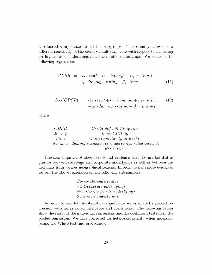
a balanced sample size for all the subgroups. This dummy allows for adifferent sensitivity of the credit default swap rate with respect to the ratingfor highly rated underlyings and lower rated underlyings. We consider thefollowing regressions

CDSR = cons tan t+ α0 · dummy1 + α1 · rating +α2 · dummy1 · rating + β2 · time+ ε (11)

Log (CDSR) = cons tan t+ α0 · dummy1 + α1 · rating (12)

+α2 · dummy1 · rating + β2 · time+ ε

where

CDSR Credit default Swap rateRating Credit RatingTime Time to maturity in weeksdummy1 dummy variable for underlyings rated below A

ε Error term

Previous empirical studies have found evidence that the market distin-guishes between sovereign and corporate underlyings as well as between un-derlyings from various geographical regions. In order to gain more evidence,we run the above regression on the following sub-samples:

Corporate underlyingsUS Corporate underlyingsNon US Corporate underlyingsSovereign underlyings

In order to test for the statistical signifcance we estimated a pooled re-gression with unrestricted intercepts and coefficients. The following tablesshow the result of the individual regressions and the coefficient tests from thepooled regression. We have corrected for heteroskedasticity when necessary(using the White test and procedure).

29

Dependent VariableExplanatory Variables Whole Sample Corporate

CDSR Log(CDSR) CDSR Log(CDSR)Constant -0.0043 -7.1393 0.0002 -6.9657

(0.05) (0.00) (0.92) (0.00)Dummy 1 -0.0035 0.6556 -0.0043 0.4376

(0.83) (0.36) (0.78) (0.51)

Rating 0.0016 0.2394 0.0012 0.2063(0.00) (0.00) (0.00) (0.00)

Rating*Dummy1 0.0013 -0.0381 0.0012 -0.0174(0.37) (0.54) (0.38) (0.76)

Time 0.0000 0.0042 0.0000 0.0036(0.64) (0.01) (0.28) (0.10)

Adjusted R2 0.40 0.55 0.35 0.50

White correction x x x x

Number of Observations 346 346 279 279

F-Statistic 57.8900 104.7700 38.2000 70.0100(0.00) (0.00) (0.00) (0.00)

Dependent VariableExplanatory Variables Corporate US Corporate Non US Sovereign

CDSR Log(CDSR) CDSR Log(CDSR) CDSR Log(CDSR)Constant -0.0009 -6.8191 0.0009 -7.1543 -0.0083 -7.1172

(0.51) (0.00) (0.82) (0.00) (0.12) (0.00)Dummy 1 -0.0393 -1.7593 0.0198 2.0609 -0.1185 -0.2098

(0.00) (0.00) (0.58) (0.11) (0.04) (0.96)

Rating 0.0009 0.1784 0.0015 0.2346 0.0022 0.2722(0.00) (0.00) (0.00) (0.00) (0.00) (0.00)

Rating*Dummy1 0.0037 0.1453 -0.0007 -0.1487 0.0126 0.0759

(0.00) (0.01) (0.83) (0.21) (0.01) (0.82)

Time 0.0000 0.0035 -0.0001 0.0045 0.0001 0.0033(0.99) (0.14) (0.27) (0.19) (0.14) (0.17)

Adjusted R2 0.68 0.50 0.37 0.55 0.63 0.66

White correction x x

Number of Observations 145 145 134 134 67 67

F-Statistic 77.4400 37.7100 20.9400 42.3000 29.2300 32.8400(0.00) (0.00) (0.00) (0.00) (0.00) (0.00)

Table 2: Results of the estimation of the following equation on the wholesample and the subgroups (on the credit default Swap rate and the log of it):CDSR = cons tan t+ α0 · dummy1 + α1 ·Rating + α2 · dummy1 ·Rating +β1 · Time

30

The first obvious result lies in the striking significance of the differentregressions, with Fisher tests never under 20. This significance is notablylinked to the significance of the ratings variable that remains strongly signifi-cant whatever the specification (linear or semi-log) and the sample considered(sovereign, US or nonUS corporates). The strongest impact economically ofratings happens with Sovereign credit default swap rates (with the largestcoefficient in both specifications). This confirms the result already in theliterature that Sovereign and Corporate ratings are not interchangeable andthat the Sovereign rating differences are larger (from a pricing point of view)than the Corporates ones.

The use of the dummy variable multiplied by the rating is a way of testingwhether low rated underlyings, whether Sovereign or Corporates, have a dif-ferent price-rating relationship than highly rated underlyings. The coefficientis only significant for the US Corporate sub-sample (and for the Sovereignsub-sample in the linear regression). The value of the coefficient of the rat-ing variable multiplied by the dummy is quite larger than the value of thecoefficient of the rating variable on its own in the linear specification, thusindicating a potentially very strong threshold impact of ratings. This indeedindicates that the influence of the rating on the level of the credit defaultswap rate varies significantly for low rated underlyings and high rated under-lyings. This can be considered in line with some theoretical results from thestructural form literature, which predict that low rated riskier debt behavessignificantly differently from high rated debt. We find the same evidencein the sovereign sub-sample with the same magnitude of impact of a ratingchange for low rated debt in the linear specification. This variable is notsignificant for the rest of the sub-samples. It may be a first hint that USCorporates ratings may behave or be considered differently from the non USones in the Credit Risk pricing market. This is due to the fact that non USCorporates include a wide range of underlyings for which credit risk pricingdoes not react in the same way to changes in their rating. Ratings do differas far as their pricing impact on credit risk in the US versus non US Corpo-rates. One should thus be wary of importing models fitted in one sample foruse in the other sample.

The time to maturity is nearly never significant. It has a positive coeffi-cient in the case where it is significant (whole sample in semi-log configura-tion), meaning that a longer time to maturity leads to a higher CDS rate (or

31

higher credit risk). The reason for the overall lack of significance might becoming from the fact that we are working on initial offering prices of CDS.The standard maturity of these contracts is 5 years. About half of our ob-servations have a time to maturity of five years or a value very close to 5years. We have also tested for the impact of a variable constituted of thedummy variable multiplied by the time variable. The idea is to test whetherthe maturity has a different impact for low rated underlyings and for highrated underlyings, as would be expected from structural form models. Wedid not obtain significant results, which may point once more to a sampleproblem as far as maturity is concerned. Finally we have tested the possibil-ity that the influence of time is more complicated than assumed by a simpleregression. We have introduced dummies for various time bands. Howeverthe more complicated structure did not yield any better results. Nearly allof the coefficients were insignificant. The reason for this could be the sameas mentioned above.

Our next regressions investigate more precisely the presence of non lineareffects in ratings. We first regress our CDS spreads on credit rating dum-mies representing rating classes (whenever we had enough observations wehave done the same test at the one-notch difference instead of the one-classdifference with similar results). We have each time omitted the worst ratingclass so that the constant in the regression represents the coefficient to thatclass. Table 3 gives the results. On the whole sample, each rating class ap-pears significant except for one. High ratings have a negative coefficient asexpected (lower spread than the worst class) but non linearities appear (thetop 3 classes do not differ much from each other while the lower classes clearlydiffer from the higher ones). Nonetheless some incongruities (such as the factthat the BB class requires a higher spread than the B class) may be linked tothe mix of truly different data such as sovereign, US and non US corporates.Regressions on each sample separately show strongly different behaviors foreach subsample. In US corporates, there is a clear distinction (that we willuse further) between high (AAA to A) and low (BBB and lower) ratings,with seemingly no strong difference between the high ratings (except for theAAA class that stands somewhat out) and no strong difference between thelow ratings (although these non significant differences are ordered in meansas expected). This further reveals the strong threshold effect that exists inUS corporate ratings.Ratings’ impact on nonUS corporates spreads is somewhat more erratic

32

and bears less explanatory power, confirming results already found in thelinear expression. Sovereign underlyings produce an almost picture perfectregression of what would expect from ratings’ impact, with a significant im-pact of each class, close to linear differences from one class to the other(except for the closeness of the two top classes) and a strong overall explana-tory power. Ratings do matter for sovereign underlyings, their impact isconsistent with common expectations and threshold effects do not seem asimportant as for US corporates.

33

Dependent VariableExplanatory Variables Whole Sample Corporate

CDSR Log(CDSR) CDSR Log(CDSR)Constant 0.0131 -4.8999 0.0131 -4.8999

(0.00) (0.00) (0.00) (0.00)AAA -0.0109 -4.8999 -0.0115 -1.5646

(0.00) (0.00) (0.00) (0.00)AA -0.0103 -1.1054 -0.0103 -1.0682

(0.00) (0.00) (0.00) (0.00)A -0.0092 -0.7982 -0.0093 -0.8219

(0.00) (0.00) (0.00) (0.00)BBB 0.0001 0.2158 -0.0009 0.1176

(0.98) (0.30) (0.78) (0.58)

BB 0.0199 1.3484 0.0075 0.8927(0.00) (0.00) (0.12) (0.00)

Adjusted R2 0.33 0.47 0.20 0.38



F-Statistic 39.2339 70.0181 17.3403 41.2900(0.00) (0.00) (0.00) (0.00)

Dependent VariableExplanatory Variables Corporate US Corporate Non US Sovereign

CDSR Log(CDSR) CDSR Log(CDSR) CDSR Log(CDSR)Constant 0.0156 -4.9194 0.0121 -4.8915 0.0405 -3.2781

(0.00) (0.00) (0.00) (0.00) (0.00) (0.00)

AAA -0.0139 -1.5451 -0.0380 -2.7680(0.00) (0.00) (0.00) (0.00)

AA -0.0124 -0.9374 -0.0095 -1.1976 -0.0394 -3.6089(0.01) (0.05) (0.01) (0.00) (0.00) (0.00)

A -0.0122 -0.8982 -0.0077 -0.7081 -0.0351 -2.1909(0.01) (0.06) (0.03) (0.00) (0.00) (0.00)

BBB -0.0077 -0.1287 0.0048 0.3920 -0.0248 -1.1553(0.12) (0.79) (0.28) (0.10) (0.00) (0.00)

BB -0.0018 0.4499 0.0119 1.1156(0.81) (0.49) (0.03) (0.00)

Adjusted R2 0.29 0.31 0.22 0.46 0.50 0.61

White correction x x x x x x


F-Statistic 14.5118 16.0229 12.0659 33.7427 18.1860 27.4515(0.00) (0.00) (0.00) (0.00) (0.00) (0.00)

Table 3: Results of the estimation of the following equation on the wholesample and the subgroups (on the credit default Swap rate and the log of it):CDSR = cons tan t + AAA · dummy + AA · dummy + A · dummy + BBBdummy +BB dummy

34

Overall, it is remarkable that with ratings only we are able to explain up to67 percent of the variation in our sample (and a minimum of 27 percent). Thehighest values are observed for the sovereign sub-sample. It is also noticeablethat our subsamples vary widely in behaviors, US corporates presenting aclear threshold effect in ratings, sovereign being influenced quasi linearly andnon US corporates presenting the least clear relationship to ratings. Andit becomes very clear that large variations in the sample, and notably inthe corporate samples, are not explained by the rating. Investigating howsuccessful other variables will be at approximating Credit Default Swap ratesremains thus important.

35

6.2 The US interest rate, the slope of the yield curveand the credit spread

Most of the empirical papers predict an increase in the credit spread if thelevel of interest rate decreases. Other interest rate variables can be consideredfor which interpretation may be more complex. The influence of the slopeof the yield curve can be seen as a proxy for the state of the economy. Asteeper term structure of interest rates is associated with an improvementof the business climate while a flatter term structure would be associatedwith a decrease in the economic activity. We have also considered the spreadbetween longterm AAA corporate bonds and longterm government bondswhich is a direct measure for the riskiness of this rating class in the US (andthus a measure of minimal credit risk). In order to investigate the relationshipwe estimate the following equation:

CDSR = cons tan t+ α0 · dummy1 + α1 · rating+α2 · dummy1 · rating + β1 · short_US+β2 · slope+ β3 · Spread+ β4 · time+ ε (13)

Log (CDSR) = cons tan t+ α0 · dummy1 + α1 · rating+α2 · dummy1 · rating + β1 · short_US+β2 · slope+ β3 · Spread+ β4 · time+ ε (14)

where

short_US level of the US short rateslope Slope of the yield curve defined as long rate− short rateSpread

Spread of the average US AAA rated bond over thelong government rate

The following table depicts the correlation of the three interest rate vari-ables for all the groups.

36

Whole SampleShort rate Slope AAA Spread

Short rate 1.0000 -0.4238 -0.7241Slope -0.4238 1.0000 0.7736AAA Spread -0.7241 0.7736 1.0000

CorporateShort rate Slope AAA Spread


SovereignShort rate Slope AAA Spread


US CorporateShort rate Slope AAA Spread


Non US CorporateShort rate Slope AAA Spread


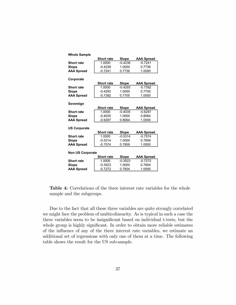
Table 4: Correlations of the three interest rate variables for the wholesample and the subgroups.

Due to the fact that all these three variables are quite strongly correlatedwe might face the problem of multicolinearity. As is typical in such a case thethree variables seem to be insignificant based on individual t-tests, but thewhole group is highly significant. In order to obtain more reliable estimatesof the influence of any of the three interest rate variables, we estimate anadditional set of regressions with only one of them at a time. The followingtable shows the result for the US sub-sample.

37

Dependent VariableExplanatory Variables US Corporate US Corporate US Corporate US Corporate

CDSR Log(CDSR) CDSR Log(CDSR) CDSR Log(CDSR) CDSR Log(CDSR)Constant -0.0110 -8.1623 0.0066 -5.4475 -0.0032 -7.1951 -0.0092 -8.2221

(0.15) (0.00) (0.02) (0.00) (0.07) (0.00) (0.00) (0.00)Dummy 1 -0.0370 -1.5257 -0.0418 -2.2112 -0.0365 -1.3097 -0.0393 -1.7526

(0.00) (0.01) (0.00) (0.00) (0.00) (0.02) (0.00) (0.00)Rating 0.0010 0.1977 0.0010 0.1898 0.0010 0.1864 0.0011 0.2010

(0.00) (0.00) (0.00) (0.00) (0.00) (0.00) (0.00) (0.00)Rating* Dummy 1 0.0035 0.1254 0.0039 0.1822 0.0035 0.1108 0.0037 0.1424

(0.00) (0.02) (0.00) (0.00) (0.00) (0.04) (0.00) (0.01)US Short Rate 0.0454 2.3858 -0.1407 -25.7281

(0.57) (0.82) (0.00) (0.00)Slope 0.7023 88.5725 1.3391 213.3073

(0.12) (0.21) (0.00) (0.00)Spread AAA 0.4229 69.2721 0.5452 91.6958

(0.11) (0.06) (0.00) (0.00)Time 0.0000 0.0035 0.0000 0.0012 0.0000 0.0036 0.0000 0.0031

(0.85) (0.14) (0.46) (0.60) (0.96) (0.10) (0.93) (0.15)

Adjusted R2 0.72 0.58 0.70 0.55 0.72 0.57 0.72 0.58

White correction x x x

Number of Observations 145 145 145 145 145 145 145 145

F-Statistic 53.3400 29.3500 67.0600 35.6700 73.4300 39.1500 73.9500 40.8800(0.00) (0.00) (0.00) (0.00) (0.00) (0.00) (0.00) (0.00)

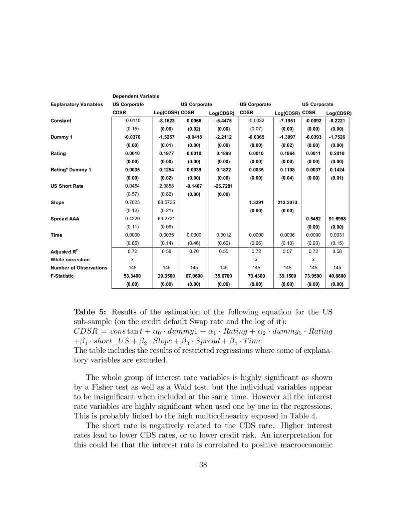
Table 5: Results of the estimation of the following equation for the USsub-sample (on the credit default Swap rate and the log of it):CDSR = cons tan t + α0 · dummy1 + α1 · Rating + α2 · dummy1 · Rating+β1 · short_US + β2 · Slope+ β3 · Spread+ β4 · TimeThe table includes the results of restricted regressions where some of explana-tory variables are excluded.

The whole group of interest rate variables is highly significant as shownby a Fisher test as well as a Wald test, but the individual variables appearto be insignificant when included at the same time. However all the interestrate variables are highly significant when used one by one in the regressions.This is probably linked to the high multicolinearity exposed in Table 4.The short rate is negatively related to the CDS rate. Higher interest

rates lead to lower CDS rates, or to lower credit risk. An interpretation forthis could be that the interest rate is correlated to positive macroeconomic

38

prospects. Interestingly though, the impact of the short rate on the CDSrate of US corporates is much higher for highly rated corporates than forlow rated corporates where it becomes insignificant. This may be linked tothe fact that low rated corporates are very sensitive to their financing costswhich increase significantly as rates increase. It shows that interest rates’impact on credit risk matters overall but is rather complex.The AAA spread has a positive sign as expected. Therefore we confirm

the findings of previous empirical research for the US sub-sample. The ad-justed R2 of the regressions increases significantly due to the inclusion ofthe interest rate variables. Therefore a pricing model of credit default swapsshould include at least some information related to the rating and the interestrate environment. However all the three interest rate variables have similarexplanatory power for the US sub-sample. Therefore we can not concludethat one is more important that the other two,as we could have expectedfrom their high correlations. The results of the estimation for the wholesample are shown below.

39

Dependent VariableExplanatory Variables Whole Sample Whole Sample Whole Sample Whole Sample

CDSR Log(CDSR) CDSR Log(CDSR) CDSR Log(CDSR) CDSR Log(CDSR)Constant 0.0193 -5.6583 0.0137 -5.2813 -0.0045 -7.3613 -0.0121 -8.3492

(0.04) (0.00) (0.00) (0.00) (0.08) (0.00) (0.01) (0.00)Dummy 1 -0.0096 0.3088 -0.0072 0.2758 -0.0034 0.8212 -0.0034 0.6787

(0.58) (0.68) (0.67) (0.71) (0.84) (0.24) (0.84) (0.33)

Rating 0.0017 0.2552 0.0017 0.2544 0.0016 0.2449 0.0017 0.2530(0.00) (0.00) (0.00) (0.00) (0.00) (0.00) (0.00) (0.00)

Rating* Dummy 1 0.0018 -0.0111 0.0016 -0.0087 0.0013 -0.0512 0.0013 -0.0395(0.25) (0.86) (0.28) (0.89) (0.38) (0.39) (0.37) (0.51)

US Short Rate -0.4204 -32.7086 -0.3499 -36.0653(0.00) (0.00) (0.00) (0.00)

Slope -1.2510 -4.7787 0.0896 124.7125(0.09) (0.93) (0.88) (0.00)

Spread AAA 0.0143 14.4605 0.5278 82.3000(0.97) (0.64) (0.03) (0.00)

Time 0.0000 0.0031 0.0000 0.0031 0.0000 0.0042 0.0000 0.0038(0.98) (0.04) (0.92) (0.05) (0.64) (0.01) (0.69) (0.01)

Adjusted R2 0.43 0.60 0.43 0.60 0.40 0.56 0.40 0.58

White correction x x x x x x x


F-Statistic 38.2300 74.7200 52.5400 105.0600 46.1800 87.9600 47.8300 96.1900(0.00) (0.00) (0.00) (0.00) (0.00) (0.00) (0.00) (0.00)

Table 6: Results of the estimation of the following equation for the wholesample (on the credit default Swap rate and the log of it):CDSR = cons tan t + α0 · dummy1 + α1 · Rating + α2 · dummy1 · Rating+β1 · short_US + β2 · Slope+ β3 · Spread+ β4 · TimeThe table includes the results of restricted regressions where some of explana-tory variables are excluded.

Only the US short rate is significant when we use all the three variablesin the same regression. The whole group on the other hand has a significantinfluence in all the sub-samples. The individual regressions show a differentpicture. For the whole sample all of the interest rate variables are significantexcept the US slope in the linear regressions. For the non US corporateand the sovereign underlyings only the US short rate remains consistentlysignificant. The US slope and the AAA spread lose their significance. Thisresult is interesting as it indicates that for non US underlyings the US rate

40

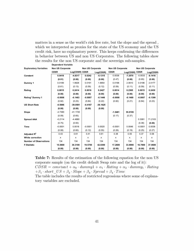
matters in a sense as the world’s risk free rate, but the slope and the spread ,which we interpreted as proxies for the state of the US economy and the UScredit risk, have no explanatory power. This keeps confirming the differencesin behavior between US and non US Corporates. The following tables showthe results for the non US corporate and the sovereign sub-samples.

Dependent VariableExplanatory Variables Non US Corporate Non US Corporate Non US Corporate Non US Corporate

CDSR Log(CDSR) CDSR Log(CDSR) CDSR Log(CDSR) CDSR Log(CDSR)Constant 0.0418 -4.8317 0.0242 -5.1315 0.0038 -7.2570 -0.0033 -8.1416

(0.01) (0.00) (0.00) (0.00) (0.47) (0.00) (0.65) (0.00)Dummy 1 0.0189 1.9928 0.0191 1.9954 0.0198 2.0610 0.0196 2.0177

(0.61) (0.13) (0.59) (0.12) (0.59) (0.11) (0.59) (0.11)

Rating 0.0015 0.2414 0.0016 0.2427 0.0014 0.2365 0.0015 0.2430(0.00) (0.00) (0.00) (0.00) (0.00) (0.00) (0.00) (0.00)

Rating* Dummy 1 -0.0008 -0.1463 -0.0007 -0.1448 -0.0008 -0.1469 -0.0007 -0.1399(0.82) (0.23) (0.84) (0.22) (0.82) (0.21) (0.84) (0.23)

US Short Rate -0.5886 -39.0581 -0.4167 -36.1625(0.00) (0.00) (0.00) (0.00)

Slope -2.7390 -41.1720 -1.5481 55.9195(0.09) (0.65) (0.17) (0.37)

Spread AAA -0.2114 -4.4880 0.3081 71.2103(0.75) (0.93) (0.38) (0.00)

Time -0.0001 0.0018 -0.0001 0.0020 -0.0001 0.0046 -0.0001 0.0038(0.08) (0.60) (0.12) (0.55) (0.26) (0.19) (0.25) (0.27)

Adjusted R2 0.43 0.61 0.41 0.61 0.38 0.55 0.37 0.58

White correction x x x x x x x x


F-Statistic 15.5800 30.3100 19.5700 42.8300 17.2600 33.8900 16.7800 37.0600(0.00) (0.00) (0.00) (0.00) (0.00) (0.00) (0.00) (0.00)

Table 7: Results of the estimation of the following equation for the non UScorporate sample (on the credit default Swap rate and the log of it):CDSR = cons tan t + α0 · dummy1 + α1 · Rating + α2 · dummy1 · Rating+β1 · short_US + β2 · Slope+ β3 · Spread+ β4 · TimeThe table includes the results of restricted regressions where some of explana-tory variables are excluded.

41

Explanatory Variables SovereignCDSR Log(CDSR) CDSR Log(CDSR) CDSR Log(CDSR) CDSR Log(CDSR)

Constant 0.0821 -0.4657 0.0317 -3.6534 -0.0066 -7.1548 -0.0106 -7.8869(0.00) (0.70) (0.00) (0.00) (0.26) (0.00) (0.32) (0.00)

Dummy 1 -0.1572 -2.6727 -0.1239 -0.6769 -0.1231 -0.1083 -0.1164 0.4946

(0.00) (0.31) (0.17) (0.84) (0.03) (0.98) (0.05) (0.90)

Rating 0.0031 0.3503 0.0030 0.3454 0.0021 0.2734 0.0022 0.2817(0.00) (0.00) (0.00) (0.00) (0.00) (0.00) (0.00) (0.00)

Rating* Dummy 1 0.0154 0.2431 0.0125 0.0698 0.0130 0.0666 0.0124 0.0071

(0.00) (0.31) (0.12) (0.82) (0.01) (0.84) (0.02) (0.98)

US Short Rate -1.4214 -109.8740 -0.9105 -78.8030(0.00) (0.00) (0.00) (0.00)

Slope -1.4794 -45.0359 -0.9462 20.9506(0.41) (0.67) (0.48) (0.81)

Spread AAA -1.6471 -113.5704 0.1515 50.2066(0.08) (0.04) (0.80) (0.20)

Time 0.0001 0.0066 0.0001 0.0057 0.0001 0.0033 0.0001 0.0034

(0.00) (0.00) (0.00) (0.00) (0.13) (0.18) (0.14) (0.16)

Adjusted R2 0.77 0.84 0.72 0.80 0.63 0.65 0.63 0.66

White correction x


F-Statistic 32.0900 49.2500 35.0700 55.0800 23.3000 25.8800 23.0400 26.8800(0.00) (0.00) (0.00) (0.00) (0.00) (0.00) (0.00) (0.00)

Table 8: Results of the estimation of the following equation for the sovereignsample (on the credit default Swap rate and the log of it):CDSR = cons tan t + α0 · dummy1 + α1 · Rating + α2 · dummy1 · Rating+β1 · short_US + β2 · Slope+ β3 · Spread+ β4 · TimeThe table includes the results of restricted regressions where some of explana-tory variables are excluded.

42

6.3 The influence of foreign interest rates

We have found evidence that the slope of the US yield curve is significantfor the US sub-sample. However it is not significant for non US underlyings.We want to test for the influence of non US interest rates. We have testedfor the influence of the levels and the slopes of the yield curves of the fol-lowing countries: Australian rates for Australian companies, Japanese ratesfor Asian companies, German rates for countries of continental Europe andBritish Pound rates for underlyings in the UK. The rates and the slopes ofthe individual country rates are highly correlated and we encounter the samekind of multicolinearity problems as with the US interest rate. Therefore werestrict ourselves to use only the level of the US short rate and the slopes ofthe individual country yield curves. We estimate the following equations:

CDSR = cons tan t+ α0 · dummy1 + α1 · rating + α2 · dummy1 · rating+β3 · short_US + β4 ·Au ·AuSlope+ β5 ·Ge ·GeSlope+β6 · JP · JpSlope+ β7UK · UKSlope+ βTime+ ε (15)

Log (CDSR) = cons tan t+ α0 · dummy1 + α1 ·Rating + α2 · dummy1·Rating + β3 · short_US + β4 ·Au ·AuSlope+β5 ·Ge ·GeSlope+ β6 · JP · JpSlope+β7 · UK · UKSlope+ β8 · Time+ ε (16)

whereshort_US level of the US short rateAu, Ge, Jp, UK Country DummiesAu, Ge, Jp, UKSlope Country Slopes

The results of the regressions are shown in the following table.

43

Dependent VariableExplanatory Variables Whole Sample Sovereign Corporate Non US Corporates

CDSR Log(CDSR) CDSR Log(CDSR) CDSR Log(CDSR) CDSR Log(CDSRConstant 0.0111 -5.5091 0.0199 -4.8481 0.0113 -5.5887 0.0222 -5.1642

(0.01) (0.00) (0.05) (0.00) (0.02) (0.00) (0.00) (0.00)Dummy 1 -0.0038 0.4674 -0.1291 -0.6333 -0.0038 0.2400 0.0209 1.8121

(0.82) (0.54) (0.01) (0.77) (0.82) (0.75) (0.55) (0.03)Rating 0.0017 0.2524 0.0026 0.3584 0.0012 0.1957 0.0015 0.2029

(0.00) (0.00) (0.00) (0.00) (0.00) (0.00) (0.00) (0.00)Rating*Dummy1 0.0013 -0.0285 0.0128 0.0398 0.0012 0.0072 -0.0010 -0.1385

(0.39) (0.66) (0.00) (0.84) (0.40) (0.91) (0.75) (0.08)

US Short Rate -0.2937 -30.7614 -0.5240 -51.0116 -0.2000 -23.4939 -0.2956 -24.1472(0.00) (0.00) (0.01) (0.00) (0.01) (0.00) (0.02) (0.00)

AU*Slope AU -2.7650 -144.7317 -1.8419 -92.9712 -4.6663 -305.7934(0.01) (0.03) (0.03) (0.13) (0.00) (0.00)

GE*Slope GE -0.4423 -55.0117 -1.9272 -139.8780 -0.1062 -51.2254 -1.5239 -176.5203(0.00) (0.00) (0.00) (0.00) (0.43) (0.00) (0.00) (0.00)

JP*Slope JP 0.1640 31.3538 -0.6099 48.7801 0.4862 56.1647 -0.6186 -29.2604(0.52) (0.07) (0.57) (0.35) (0.07) (0.00) (0.07) (0.27)

UK*Slope UK 0.3485 37.9199 0.0764 21.6882 1.2258 125.4778(0.06) (0.08) (0.70) (0.30) (0.00) (0.00)

Time 0.0000 0.0036 0.0001 0.0053 -0.0001 0.0025 -0.0001 0.0044(0.75) (0.02) (0.01) (0.00) (0.19) (0.29) (0.22) (0.11)

Adjusted R2 0.44 0.37 0.56 0.45 0.70

White correction x x x x x


F-Statistic 30.8300 63.1900 33.0300 77.3600 19.2300 39.9600 13.3200 34.7000(0.00) (0.00) (0.00) (0.00) (0.00) (0.00) (0.00) (0.00)

Table 9: Results of the estimation of the following equation for the wholesample and all the subgroups (on the credit default Swap rate and the log ofit):CDSR = cons tan t+ α0 · dummy1 + α1 ·Rating + α2 · dummy1 ·Rating +β3 · short_US + β4 ·Au ·AuSlope+ β5 ·Ge ·GeSlope+ β6 · JP · JpSlope+β7UK · UKSlope+ β8Time

In general we find that the level of the short term US rate remains signif-icant through out all the sub-samples. All the additional yield curve slopesare significant except the Japanese slope. The Japanese slope is significantfor the corporate sub-sample including or excluding US corporations. It ishowever not significant for the sovereign and the overall sample. The reasonfor the insignificance in the sovereign sub-sample might be due to the fact

44

that there are only five observations of credit default swaps on the Japanesegovernment. The signs of the coefficient are as expected for the Australianand the German slopes. They are positive and thus support the view thata steeper yield curve is associated with improving business conditions, andthus associated with lower credit risk. The coefficient of the Japanese slopechanges sign but is insignificant and thus we can not draw any additionalconclusions. The sign of the UK slope is negative, while we observed aninverted term structure for the whole sample period in the UK.

We find evidence that the US interest rate has a strong influence on creditdefault swap rates even after controlling for the effects of the local termstructure. The slope of the local term structure adds additional information.We have interpreted the slope of the yield curve as an indicator of futureeconomic conditions. As the US and the rest of the world are not at the samestage in the business cycle, the economic outlook for the various economiesis different. The finding that the slope of the local interest rates matter isconsistent with this interpretation.

45

6.4 The variance

Although we do not test for any specific models in this paper, it is interestingto investigate further stylized facts expected from theoretical models. Mostof the structural form models predict that an increase in the variability of thefirm’s asset value leads to higher credit risk. We use the historical varianceas a proxy for the variability of the firm value. All the variables used sofar were not firm specific. Even if the rating encompasses theoretically allthe relevant information contained in the stock price, it is a very sluggishmeasure of credit quality. The information contained in the stock price getsupdated almost instantly on the arrival of new information relevant to theunderlying firm. Therefore we expect that the variance and the other stockprice related variables add information because they are firm specific and upto date. Variance and other stock related variables are at the center of thestructural form models of credit risk (and can be incorporated in reducedform models).

We estimate the following equation

CDSR = cons tan t+ α0 · dummy1 + α1 ·Rating (17)

+α2 · dummy1 ·Rating + β1 · short_US+β4 · V ar + β5 · Time+ ε

Log (CDSR) = cons tan t+ α0 · dummy1 + α1 ·Rating (18)

+α2 · dummy1 ·Rating + β1 · short_US+β4 · V ar + β5 · Time+ ε

whereV ar Annualized variance of the stock returns

The following table depicts the results of the regressions.

46

Dependent VariableExplanatory Variables Corporate US Corporate Non US Corporate


(0.03) (0.00) (0.13) (0.00) (0.15) (0.00)Dummy 1 -0.0116 -0.3367 -0.0326 -1.1074 0.0258 1.2656

(0.45) (0.61) (0.00) (0.08) (0.61) (0.53)

Rating 0.0012 0.2192 0.0012 0.2106 0.0010 0.2312(0.00) (0.00) (0.00) (0.00) (0.00) (0.00)

Rating*Dummy1 0.0014 0.0152 0.0029 0.0653 -0.0015 -0.1102(0.24) (0.78) (0.00) (0.26) (0.72) (0.52)

US Short Rate -0.2095 -26.5179 -0.1667 -28.7906 -0.1671 -24.3960(0.00) (0.00) (0.00) (0.00) (0.14) (0.00)

Variance 0.0345 1.8661 0.0192 2.3548 0.0412 1.7225(0.00) (0.00) (0.01) (0.00) (0.00) (0.00)

Time -0.0001 0.0016 0.0000 0.0020 -0.0001 0.0009(0.14) (0.47) (0.70) (0.38) (0.12) (0.84)

Adjusted R2 0.56 0.62 0.76 0.61 0.56 0.63



F-Statistic 51.8393 66.2826 68.8475 35.1568 24.1007 32.5349(0.00) (0.00) (0.00) (0.00) (0.00) (0.00)

Table 10: Results of the estimation of the following equation for the corpo-rate sub-samples (on the credit default Swap rate and the log of it):CDSR = cons tan t+ α0 · dummy1 + α1 ·Rating + α2 · dummy1 ·Rating +β3 · short_US + β4 · V ariance+ β5Time

47

Dependent VariableExplanatory Variables US High US Low Non US High Non US Low

CDSR Log(CDSR) CDSR Log(CDSR) CDSR Log(CDSR) CDSR Log(CDSR)Constant 0.0071 -5.0643 -0.0037 -5.0721 0.0013 -6.4395 0.0381 -3.4724

(0.00) (0.00) (0.67) (0.00) (0.58) (0.00) (0.20) (0.01)Rating 0.0003 0.0891 0.0022 0.1416 0.0006 0.1729 0.0017 0.1348

(0.08) (0.05) (0.00) (0.00) (0.00) (0.00) (0.18) (0.04)US Short Rate -0.1227 -29.5465 -0.2148 -29.5358 -0.0543 -14.8300 -0.4678 -38.8352

(0.00) (0.00) (0.15) (0.02) (0.13) (0.09) (0.05) (0.00)Variance 0.0043 0.8057 0.0354 3.3696 0.0017 0.4566 0.0411 1.7132

(0.17) (0.29) (0.00) (0.00) (0.48) (0.45) (0.00) (0.03)Time 0.0000 0.0042 0.0000 -0.0025 0.0000 0.0078 -0.0004 -0.0129

(0.64) (0.11) (0.36) (0.56) (0.04) (0.02) (0.14) (0.29)

Adjusted R2 0.16 0.20 0.69 0.54 0.27 0.32 0.59 0.51



F-Statistic 4.8220 5.9119 28.7181 15.2710 7.7096 9.5905 13.2807 9.7422(0.00) (0.00) (0.00) (0.00) (0.00) (0.00) (0.00) (0.00)

Table 11: Results of the estimation of the following equation for the USsub-sample and the US high and low rated sub-samples (on the credit defaultSwap rate and the log of it):CDSR = cons tan t+α0 ·Rating+β3 · short_US+β4 ·V ariance+β5Time

The influence of the variance of the underlying stock price is positive andsignificant for all the sub-samples, whether US or non US Corporates, in thelinear or semi log specification. The coefficient is higher for the non US cor-porates. The contribution to the overall explanatory power of the regressionis quite high on an already remarkable level. The result is a clear indicationthat firm specific information matters and the prediction of the structuralform models is verified in our sample. Firm volatility adds information be-yond what is captured in ratings for the pricing of Credit Default Swaps.We have also tested for different shapes for the relationship. For example,we have tested the influence of the volatility with and without the variance.If the volatility is included instead of the variance it is significant and hasa positive coefficient. In combination with the variance both are significant.However the volatility has a negative coefficient. We have tested for the in-fluence of the variance raised to a higher power. However these terms arenot significant beyond the variance.

48

6.5 Stock price changes

The variance measures the overall variability of the past stock prices. Itcontains no information if the future prospects of the firm have improved orworsened. A booming firm can have the same variance as a firm on the vergeof bankruptcy. The influence of past stock prices can be seen from severalperspectives. A decrease in the stock price will lead to a smaller equityand without a reduction in the amount of outstanding debt to an increasein leverage. On the other hand a decline in the stock price can indicate aworsening in the prospects of a firm. The third possible influence is from thedemand side. A decline of the stock price might induce bondholders to seekprotection from credit risk. A stronger decline might lead to more demandan thus raise the price, e.g. the credit default swap rate.

In order to test for the information contained in the returns on the stockprior to the trading date of the credit default swap, we include the marketadjusted change in the stock price during the year before the trade. Weadjust the change in the stock price for the change in the associated marketindex. We estimate the following regressions:

CDSR = cons tan t+ α0 · dummy1 + α1 ·Rating + α2 · dummy1 ·Rating+β1 · short_US + β4 · V ar + β5 ·mch1year + β7 · Time (19)

Log (CDSR) = cons tan t+ α0 · dummy1 + α1 · rating + α2 · dummy1 ·Rating+β1 · short_US + β4 · V ar + β5 ·mch1year + β7 · Time (20)

wheremch1 year market adjusted 1 year change

We have tested different time intervals to calculate the return on the stock.In general the longer the calculation period the more significant the influence.We adjust the returns on the stock for the return on the market in order tocontrol for market wide changes in the economy. The results obtained withor without the market adjustment do not vary significantly. Moreover thechanges in the stock price remain significant and of the same sign. Marketadjusted results are somewhat more significative though, showing that un-derperformance related to the market may drive credit risk somewhat more

49

that absolute underperformance. The following table shows the results of theestimation using market adjusted changes.

Dependent VariableExplanatory Variables US Non US

CDSR Log(CDSR) CDSR Log(CDSR)Constant 0.0027 -5.8580 0.0031 -6.3358

(0.31) (0.00) (0.54) (0.00)Dummy 1 -0.0392 -1.6504 0.0244 1.1690

(0.00) (0.04) (0.62) (0.56)

Rating 0.0012 0.2095 0.0010 0.2287(0.00) (0.00) (0.01) (0.00)

Dummy 1 * Rating 0.0036 0.1186 -0.0011 -0.0821

(0.00) (0.11) (0.78) (0.63)

US Short Rate -0.1435 -26.8879 -0.0641 -17.3576(0.01) (0.00) (0.56) (0.02)

Variance 0.0175 2.2153 0.0374 1.4678(0.01) (0.00) (0.00) (0.01)

1 year changes -0.0013 -0.1103 -0.0061 -0.4157(0.01) (0.26) (0.00) (0.01)

Time 0.0000 0.0022 -0.0001 0.0012(0.83) (0.34) (0.12) (0.77)

Adjusted R2 0.76 0.61 0.59 0.66



F-Statistic 61.1148 30.3847 23.3277 30.9352(0.00) (0.00) (0.00) (0.00)

Table 12: Results of the estimation of the following equation for the USsub-samples (on the credit default Swap rate and the log of it):CDSR = cons tan t+α0 ·dummy1+α1 ·Rating+α2 ·dummy1 ·Rating+β3 ·short_US+β4 ·V ariance+β5 · 1 year market adjusted changes+β6 ·Time

The change in the stock price is significant for all the subgroups. The 1year change has a negative sign pointing to the fact that an increase in thestock price is associated with a lower credit risk while a decrease leads to ahigher risk. (We also looked at absolute changes which have positive signand are significant, even when used with relative changes, showing that both

50

the direction and the size of the change matter. We do not reproduce thesehere as absolute changes capture essentially the same element as variance orvolatility does).

51

6.6 Leverage

One of the interpretations of why past stock returns may have explanatorypower for the credit default swap rate could be linked to their effect onleverage. Most of the structural form models use the ratio of market valueof equity and debt value as an indicator of default probability (distance todefault). We use the ratio of market value of equity and debt as a proxyfor leverage. We restrict ourselves to the US sub-sample for the followingestimation for two reasons. Leverage is strongly dependent on the countryand the industry, for accounting, tax and agency reasons. A country withlarge conglomeratesincluding a house bank may view a higher leverage asmore acceptable than an economy with independent banks for agency rea-sons. Secondly as the debt value is almost always produced as an accountingnumber it depends strongly on the accounting principles used in every coun-try. In order to have a somewhat reliable number we restrict the followingestimation to the US sub-sample hoping the US accounting principle (USGAAP) provides a reliable estimate of the true leverage. We estimate thefollowing equation:

CDSR = cons tan t+ α0 · dummy1 + α1 · rating + α2 · dummy1 · rating+β1 · short_US + β4 · V ar+β5 ·mch1year + β6 · Lev + β8 · time (21)

Log (CDSR) = cons tan t+ α0 · dummy1 + α1 ·Rating + α2 · dummy1 ·Rating+β1 · short_US + β4 · V ariance+β5 ·mch1year + β6 · Lev + β8 · time (22)

where

Lev Total Liabilities/Market value of equity

Table 13 shows the results of the regressions.

52

Dependent VariableExplanatory Variables US

CDSR Log(CDSR)Constant 0.0015 -6.0825

(0.56) (0.00)Dummy 1 -0.0413 -1.7519

(0.00) (0.03)Rating 0.0012 0.2129

(0.00) (0.00)Dummy 1 * Rating 0.0037 0.1179

(0.00) (0.11)

US Short Rate -0.1340 -23.8107(0.01) (0.00)

Variance 0.0185 2.0712(0.01) (0.00)

1 year changes -0.0014 -0.0736

(0.01) (0.46)

Leverage 0.0001 0.0215(0.05) (0.00)

Time 0.0000 0.0023(0.83) (0.30)

Adjusted R2 0.78 0.64

White correction x

Number of Observations 121 121

F-Statistic 53.8643 27.2423(0.00) (0.00)

Table 13: Results of the estimation of the following equation for the USsub-sample (on the credit default Swap rate and the log of it):CDSR = cons tan t+ α0 · dummy1 + α1 ·Rating + α2 · dummy1 ·Rating +β3 · short_US+β4 ·V ariance+β5 · 1 year market adjusted changes+β6 ·Leverage+ β7 · Time

The results show that leverage has a significant influence on the creditdefault swap rates in our sample beyond the rating, interest rate and volatilityinformation. More surprisingly we note that the influence of the stock pricechanges remains significant even after controlling for the leverage effects.Overall, including the different variables, interest rate variables as well asthe firm specific variables such as variance of the value of the firm’s assets,

53

leverage and past stock price evolution improves the adjusted R2 to a highlevel of 78% in the linear form. This result confirms that the variables thatwere provided by theoretical models do explain most of the variation in creditrisk pricing.

54

6.7 The impact of liquidity as measured by marketcapitalization

As Credit Defaults Swaps constitute an exotic market where pricing is oftenattempted by replication and thus affected by the existence and the liquidityof the considered securities, we try to capture liquidity effects by a marketcapitalization proxy.We estimate the following equations

CDSR = cons tan t+ α1 ·Rating + α2 ·Market CapitalisationLog (CDSR) = cons tan t+ α1 ·Rating + α2 ·Market Capitalisationand

CDSR = cons tan t+ α1 ·Rating ++β1 · short_US+β2 · V ariance+ β3 · Leverage+β4 ·Market Capitalisation+ β5 · Time

Log (CDSR) = cons tan t+ α1 ·Rating ++β1 · short_US+β2 · V ariance+ β3 · Leverage+β4 ·Market Capitalisation+ β5 · Time

The following tables show the results of the regressions.

Dependent VariableExplanatory Variables US Corporate US High Rated US Low Rated


(0.02) (0.00) (0.00) (0.00) (0.00) (0.00)Rating 0.0016 0.1661 0.0002 0.0713 0.0031 0.2225

(0.00) (0.00) (0.15) (0.08) (0.00) (0.00)Market Capitalisation -0.0019 -3.4200 -0.0141 -3.6500 -0.0034 -1.9400

(0.85) (0.00) (0.00) (0.00) (0.94) (0.68)

Adjusted R2 0.50 0.53 0.09 0.11 0.57 0.39



F-Statistic 68.0376 75.6900 5.2564 6.2523 34.6708 16.6626(0.00) (0.00) (0.01) (0.00) (0.00) (0.00)

Table 14: Results of the estimation of the following equation for the US,the US high and low rated sub-samples (on the credit default Swap rate andthe log of it): CDSR = cons tan t+α1 ·Rating+α2 ·market capitalisation

55

Dependent VariableExplanatory Variables US

CDSR Log(CDSR)Constant -0.0038 -5.0741

(0.73) (0.00)Rating 0.0021 0.1251

(0.00) (0.00)US Short Rate -0.1984 -28.4542

(0.36) (0.14)

Variance 0.0388 3.8258(0.00) (0.00)

Leverage -0.0001 -0.0009(0.81) (0.97)

Market Capitalisation 0.0000 0.0000(0.74) (0.89)

Time 0.0000 -0.0020(0.36) (0.51)

Adjusted R2 0.69 0.55


Number of Observations 49 49

F-Statistic 18.9674 10.6315(0.00) (0.00)

Table 15: Results of the estimation of the following equation for the USsub-sample (on the credit default Swap rate and the log of it):CDSR = cons tan t + α1 · Rating + β1 · short_US + β2 · V ariance + β3 ·Leverage+ β4 ·Market Capitalisation+ β5 · Time

The proxy is significant for high rated US corporates but not for the lowrated ones. This could be a sign that liquidity effects are leading differ-ences in high rated US corporates. Nonetheless, interpretation is not secureas significance drops in multivariate regressions, notably when they includeleverage. Overall, liquidity effects as measured by this proxy do not seem toimpact prices significantly in this market.

56

6.8 The overall impact of structural variables versusratings

We further explore how structural variables (variance, leverage, time, andinterest rate) fare in predicting CDS rates versus ratings (and time). Ratingsare the most used source of information for credit risk and remain overall thesingle most useful source of explanatory power in our regressions indeed.When considering the overall sample of US Corporates for example, rat-

ings provide for a R2 of 47% in the linear form while structural variablesprovide for 31%. These structural variables are not subsumed in ratings ascombining them with ratings increases the explanatory power significantlyto 65%.Nonetheless, when considering subsamples, the picture changes and the

importance of considering structural variables becomes even stronger. Look-ing at high rated US corporates, ratings have very low explanatory power(4%) and this explanatory power is subsumed in size differences as discussedabove. On the other hand, structural variables (notably with the leveragevariable) keep a high explanatory power of 48%. Regarding low rated cor-porates on the other hand, ratings do dominate while structural variables(notably the variance variable) help boost the explanatory power, thus fur-ther illustrating the strong threshold effect that affects US corporates.We have still a different picture for non US corporates, illustrating once

more the non homogeneity of credit risk and its complexity. Ratings in nonUS corporates matter and provide most of the explanatory power for the highrated corporates while most of the explanatory power is provided by struc-tural variables (variance) for low rated corporates. Overall though, this con-firms the importance of considering structural variables in determining creditrisk spreads. Reduced form models, which have many advantages comparedto structural models, notably as far as implementation is concerned, shouldthus incorporate structural variables in the way some of the most recent suchmodels do (eg Jarrow and Turnbull (2000)). Structural models, on the otherhand, can keep instructing us on the theoretical shape of the relationshipbetween structural variables and credit risk.

57

Dependent VariableExplanatory Variables US Corporate US Corporate US Corporate


(0.46) (0.00) (0.70) (0.00) (0.04) (0.00)Rating 0.0015 0.1851 0.0015 0.1833

(0.00) (0.00) (0.00) (0.00)Short Rate -0.1119 -22.1849 -0.0178 -12.7241

(0.07) (0.00) (0.83) (0.20)

Variance 0.0301 2.1428 0.0426 3.8898(0.00) (0.00) (0.00) (0.00)

Leverage 0.0001 0.0215 0.0000 0.0066(0.06) (0.01) (0.80) (0.56)

Time 0.0000 0.0018 0.0000 -0.0019 0.0000 0.0032(0.80) (0.43) (0.19) (0.58) (0.83) (0.19)

Adjusted R2 0.65 0.61 0.31 0.18 0.47 0.48



F-Statistic 45.6770 38.0248 14.7818 7.5544 63.9601 67.9813(0.00) (0.00) (0.00) (0.00) (0.00) (0.00)

Table 16: Results of the estimation of the following equation for the UScorporate sub-sample (on the credit default Swap rate and the log of it):CDSR = cons tan t + α1 · Rating ++β1 · short_US + β2 · V ariance + β3 ·Leverage+ β5 · Time

The estimations includes restricted versions of the above equation.

58

Dependent VariableExplanatory Variables US High Rated US High Rated US High Rated


(0.00) (0.00) (0.00) (0.00) (0.45) (0.00)Rating 0.0001 0.0480 0.0003 0.1008

(0.42) (0.23) (0.05) (0.01)Short Rate -0.1172 -26.9325 -0.1154 -26.2720

(0.00) (0.00) (0.00) (0.00)Variance -0.0014 -0.4981 -0.0015 -0.5556

(0.62) (0.47) (0.58) (0.42)

Leverage 0.0002 0.0350 0.0002 0.0364(0.00) (0.00) (0.00) (0.00)

Time 0.0000 0.0034 0.0000 0.0027 0.0000 0.0075(0.88) (0.15) (0.72) (0.24) (0.12) (0.01)

Adjusted R2 0.48 0.41 0.48 0.41 0.04 0.11

White correctionNumber of Observations 72 72 72 72 93 93

F-Statistic 14.0574 10.8603 17.4979 13.1179 2.7333 6.4374(0.00) (0.00) (0.00) (0.00) (0.07) (0.00)

Table 17: Results of the estimation of the following equation for the UShigh rated sub-sample (on the credit default Swap rate and the log of it):CDSR = cons tan t + α1 · Rating ++β1 · short_US + β2 · V ariance + β3 ·Leverage+ β5 · Time


59

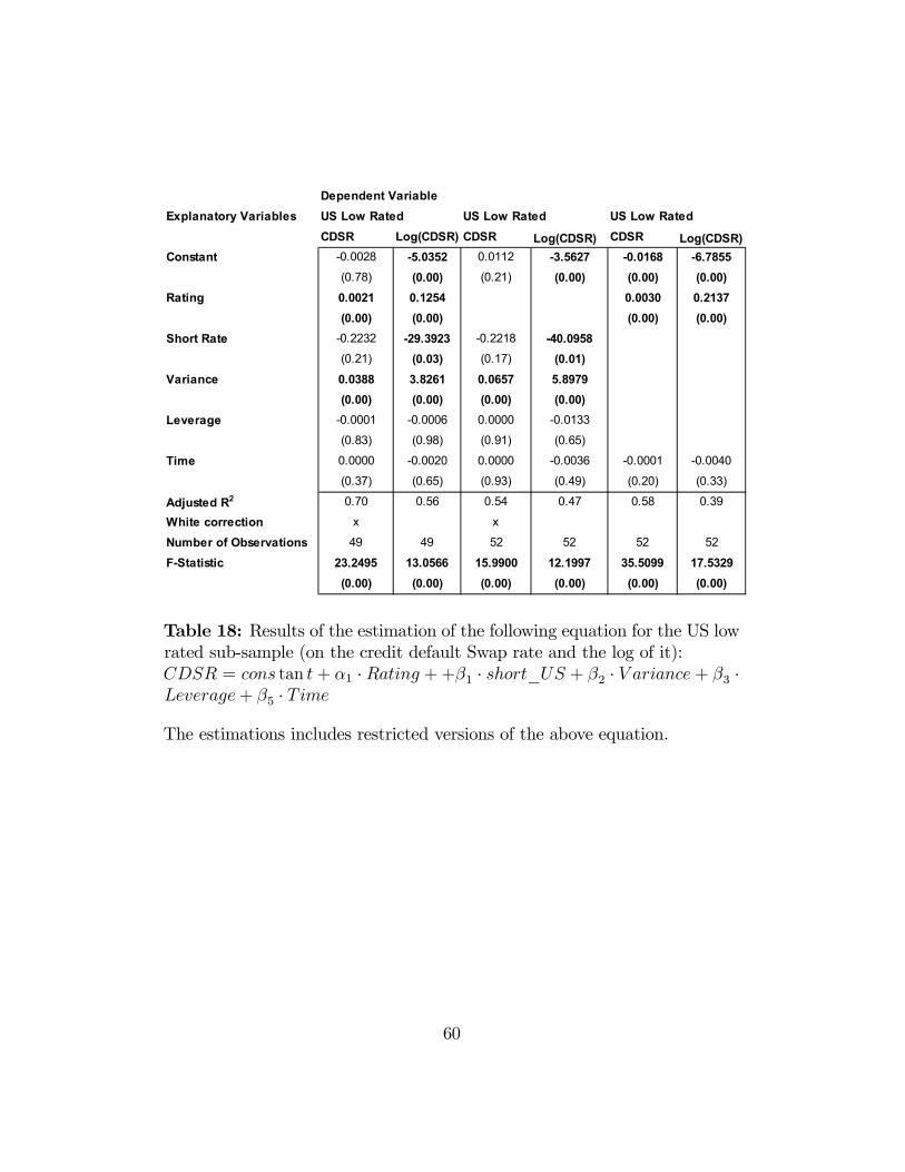
Dependent VariableExplanatory Variables US Low Rated US Low Rated US Low Rated


(0.78) (0.00) (0.21) (0.00) (0.00) (0.00)Rating 0.0021 0.1254 0.0030 0.2137

(0.00) (0.00) (0.00) (0.00)Short Rate -0.2232 -29.3923 -0.2218 -40.0958

(0.21) (0.03) (0.17) (0.01)Variance 0.0388 3.8261 0.0657 5.8979

(0.00) (0.00) (0.00) (0.00)Leverage -0.0001 -0.0006 0.0000 -0.0133

(0.83) (0.98) (0.91) (0.65)

Time 0.0000 -0.0020 0.0000 -0.0036 -0.0001 -0.0040(0.37) (0.65) (0.93) (0.49) (0.20) (0.33)

Adjusted R2 0.70 0.56 0.54 0.47 0.58 0.39



F-Statistic 23.2495 13.0566 15.9900 12.1997 35.5099 17.5329(0.00) (0.00) (0.00) (0.00) (0.00) (0.00)

Table 18: Results of the estimation of the following equation for the US lowrated sub-sample (on the credit default Swap rate and the log of it):CDSR = cons tan t + α1 · Rating ++β1 · short_US + β2 · V ariance + β3 ·Leverage+ β5 · Time


60

7 Conclusions

We have investigated the influence of various factors on Credit Default Swaprates and therefore on credit risk as reflected in a recent credit derivativemarket. This paper reflects the complexity of credit risk, a risk that is nothomogenous amongst underlyings (whether sovereigns or corporates, US andnon US based).

Starting from theoretical models, we have identified some factors thatshould influence the CDS rates. We have compared econometrically theinfluence of those factors on various subgroups in our sample. We find that allof the theoretical factors have a significant influence and that taken togetherthese factors drive much of the variation in the pricing of Credit DefaultSwaps (up to 82% despite our probably misspecified linear form).

The rating is the most important single source of information on creditrisk, although all the other factors add significant information to ratings andmatter more than ratings for some subgroups. This latter fact stresses theimportance of alternative theories such as structural form credit risk theo-ries (and the need to incorporate such variables in reduced form theories).Ratings themselves can have strong threshold effects as we find that the sen-sitivity of the level of credit default swap rates to ratings is different for highrated debt and for low rated debt. Hence a difference in rating for highquality US corporate underlyings can have close to no explanatory powerwhile structural variables such as market value leverage do have explanatorypower. In general such structural variables (variance notably for low ratedunderlyings) have explanatory power and are not subsumed in ratings. Sov-ereign and Corporates have different sensitivities to rating information andUS and non US corporates show different behaviors in relationship to ratings(with threshold effects seemingly not as significant for non US corporates asfor US corporates). US interest rates influence the credit default rates ofall the subgroups, e.g. US rates do matter for credit default swap rates ofunderlyings from other countries. For US companies the level, the slope ofthe yield curve and the spread matter. For non US underlyings the level ofthe US rates is important, however the local slope of the yield curve mat-ters more than the US slope. Considering the slope of the yield curve as anindicator of future economic activity this points to the fact that default islinked to the performance of the local economy, as would be expected. We

61

thus have further evidence that international credit risk markets are not ho-mogenous and that national markets may differ both in behavioral structure(thresholds) as well as in the variables to consider (local term structures). Aspredicted by structural models the variance of the stock price is positivelylinked with the default swap rates. It adds specific information beyond whatis contained in ratings and thus should be considered when estimating creditrisk. Declines in the stock price are positively associated with the observeddefault swap rates. We find evidence that the size and the direction of thechange in stock prices matter. Further in line with structural form modelswe find that leverage has a significant influence on the default swap rates.Even when we control for leverage and market index changes the influenceof past stock price changes remains significant. Liquidity effects as measuredby market capitalization do not seem to matter. Overall considering stochas-tic interest rates and what we call structural variables remains a necessitybeyond the use of ratings for a good approximation of credit risk.

Further research will be needed to investigate the influence of maturityfurther, explore further the threshold and other non linearities present in thevariables, and overall build a convincing and empirically practical model thatwill allow for more precise empirical testing of what drives credit risk.

62

7.1 References

- Alessandrini, F., 1999, ”Credit Risk, Interest Rate Risk, and the Busi-ness Cycle”, The Journal of Fixed Income, September 1999, p. 42 -53.

- Altman, E. and A. Saunders, 1997, ” Credit Risk Measurement: Devel-opments over the Last 20 Years ”, forthcoming in Journal of Bankingand Finance, March 1992.

- Batten, J.; Ellis, C.; Hogan,W., 1999, ”Scaling the Volatility of CreditSpreads: Evidence from the Australian Eurobonds”, Working Paper.

- Cantor, R. and Packer, F., 1996, ”Determinants and Impact of Sov-ereign Credit Ratings”, Economic Policy Review, October 1996, p. 37- 53.

- Claessens, S. and Pennacchi, G., 1996, ”Estimating the Likelihood ofMexican Default from the Market Prices of Brady Bonds”, Journal ofFinancial and Quantitative Analysis, March 1996, Vol. 31, No. 1, p.109 - 126.

- Collin-Dufresne, P. and Goldstein, R.S., 1999, ”Do Credit Spreads Re-flect Stationary Leverage Ratios? Reconciling Structural and Reduced-Form Frameworks.”, Working Paper.

- Collin-Dufresne, P.; Goldstein, R.S.; Spencer, M.J., 2000, ”The Deter-minants of Credit Spread Changes”, Working Paper.

- Cossin, Didier; Pirotte, Hugues, 1997. ”Swap Credit Risk: An Empiri-cal Investigation on Transaction Data.”. Journal of Banking & Finance.Vol. 21 (10). p1351-73. October 1997.

- Cossin, D., and H. Pirotte, 1998, ” How Well Do Classical Credit RiskModels Fit Swap Transaction Data ? ”, European Financial Manage-ment Journal, vol. 4, no 1, March 1998, p.65-78.

- Cumby, R.E. and Evans, M.D.D., 1997, ”The Term Strucutre of CreditSpreads: Estimates and Specification Tests”, Working Paper.

63

- Das, S. R. and P. Tufano, 1995, ” Pricing Credit Sensitive Debt whenInterest Rates, Credit Ratings and Credit Spreads are Stochastic ”,Journal of Financial Engineering, Vol. 5, p. 161- 198.

- Das, S. R. and Sundaram, R. K., 2000 ” A Discrete-Time Approachto Arbitrage-Free Pricing of Credit Derivatives ”, Management Science46(1), January 2000, pp. 46-63 .

- Duffie, D. and Singleton, K. J., 1997, ”An Econometric Model of theTerm Structure of Interest-Rate Swap Yields.”. Journal of Finance.Vol. 52 (4). P. 1287-1321. September 1997.

- Duffee, G.R., 1998, ” The Relationship Between Treasury Yields andCorporate Bond Yield Spreads”, The Journal of Finance, December1998, Vol. LII, N0. 6, Pp. 2225 - 2241.

- Duffee, G.R., 1999, ” Estimating the Price of Default Risk”, The Re-view of Financial Studies, Spring 1999,Vol. 12, No. 1, p. 197 -. 226.

- Dungey, M.; Martin, V.L. and Pagan A.R., 1999, ”A Multivariate La-tent Factor Decomposition of International Bond Spreads”, WorkingPaper.

- Eichengreen, B. andMody, A., 1998, ”What Explains Changing Spreadson Emerging-Market Debt: Fundamentals orMarket Sentiment?”, Work-ing Paper.

- Gho, J.C. and Ederington, L.H., 1993, ”Is a Bond Rating DowngradeBad News, Good News, or No News for Stockholders ?”, The Journalof Finance, December 1993, Vol XLVIII, No. 5, p. 2001 - 2008.

- Hettenhouse, G. W. and Sartoris, W.L., 1976, ”An Analysis of theInformational Value of Bond Rating Changes”, Quarterly Review ofEconomics and Business. 16 (2), Summer, 65-78.

- Hull, J. and White, A., 2000, ”Valuing Credit Default Swaps I: NoCounterparty Default Risk”, The Journal of Derivatives, Fall 2000.

- Hull, J. and White, A., 2000, ”Valuing Credit Default Swaps II: In-cluding Counterparty Default Risk”, The Journal of Derivatives, Fall2000.

64

- Houweling, P.; Hoek, J. and Kleibergen, F. 1999, ”The Joint Estimationof Term Structures and Credit Spreads”, Working Paper.

- Jarrow, R. and Stuart, T., 1995, ” Pricing Derivatives on FinancialSecurities Subject to Credit Risk ”, Journal of Finance, 50(1), March1995, 53-85.

- Jarrow, R.; Lando, D.and Turnbull, S. 1997, ”A Markov Model for theTerm Structure of Credit Risk Spreads”. Review of Financial Studies.Vol. 10, (2). p 481-523.

- Katz, Steven, 1974, ”The Price Adjustment Process of Bonds to Rat-ing Reclassifications: A Test of Bond Market Efficiency”, Journal ofFinance, 29 (2), May, 551-559.

- Kamin, S.B. and von Kleist, K., 1999, ”The Evolution and Determi-nants of Emerging Market Credit Spreads in the 1990’s”, BIS WorkingPaper, Nr. 68.

- Kaufold, H. and Smirlock, M., 1991, ”The Impact of Credit Risk onthe Pricing and Duration of Floatingrate Notes”, Journal of Bankingand Finance, Vol. 15, p. 43 - 52.

- Klein, P., 1996, ”Pricing Black-Scholes Options with Correlated CreditRisk”, The Journal of Banking and Finance, Vol. 20, p. 1211 - 1229.

- Leland, H. and K. Toft, 1996, ” Optimal Capital Structure, EndogenousBankruptcy, and the Term Structure of Credit Spreads ”, Journal ofFinance, 51, (July 1996), pp: 987-1019.

- Longstaff, F. and E. Schwartz, 1995, ” A Simple Approach to ValuingRisky Fixed and Floating Rate Debt ”, Journal of Finance, 50 (3), July1995.

- Longstaff, F. and E. Schwartz, 1995, ” Valuing Credit Derivatives ”,Journal of Fixed Income, June 1995, p. 6-12.

- Lopez, J.A. and Saidenberg, M.R., 1999, ”Evaluating Credit Risk Mod-els”, Working Paper.

- Lucas, D.J. and J. Lonski, 1992, ” Changes in Corporate Credit Quality1970-1990 ”, Journal of Fixed Income, March 1992.

65

- Madan D., 1998, ”Default Risk”, in Statistics in Finance by D. Haudand S. Jacker.

- Madan, D. and Unal, H., 1994, ” Pricing the Risk of Default ”, workingpaper, University of Maryland.

- Merton, R. C., 1974, ” On the pricing of corporate debt: the riskstructure of interest rates.”, Journal of Finance, Vol.29, p. 449 - 470.

- Nickell, P.; Perraudin, W. and Varotto, S. 1998, ”Stability of RatingTransitions”, Working Paper.

- Pinches, G. E. and Sinlgleton, J. C., 1978, ”The Adjustment of StockPrices to Bond Rating Changes”, The Journal of Finance, 33 (1),March, 29-44.

- Scholtes, B., 1999, ”On the Comovement of Bond Yield Spreads andCountry Risk Ratings”, The Journal of Fixed Income, March 1999, p.99- 103.

- Scott, L. 1998, ”A Note on the Pricing of Default Swaps”, WorkingPaper.

- Sutton, D.G., 1998, ”Spread Overreaction in International Bond Mar-kets”, BIS Working Paper, Nr. 55.

- Weinstein, M.I., 1977, ”The Effect of a Rating Change Announcementon the Bond Price”, Journal of Financial Economics, 5 (3), December,329 -50.

- Wilson, T. ,1997, ”Portfolio Credit Risk ”, Risk, Vol. 10 (9).

66

exploring for the determinants of credit risk in credit

Documents