exploring correlations between groundwater level change
TRANSCRIPT

Exploring correlations between Groundwater level change and settlement planning
in National Capital Territory of Delhi
A Thesis presented to the Faculty of Architecture, Planning and Preservation COLUMBIA UNIVERSITY
In Partial Fulfillment of the Requirements for the Degree
Master of Science in Urban Planning
By
Anish Pendharkar
May 2020

ii
© 2020 Anish Pendharkar

iii
ABSTRACT
Groundwater in Delhi has been decreasing continuously over the past two decades, with
many parts of the state designated as over-exploited or critically exploited. The depletion of
groundwater is often attributed to the widespread and mostly illegal extraction through tube
wells. Various case studies on water access in Delhi, point toward several factors which lead
people to use tube wells, such as the absence of piped water supply, absence of private sources of
water, inability to afford the high price of a legal connection and insecurity of tenure. These
factors result in a different level of groundwater dependence in planned and unplanned
settlements.
This is a novel exploratory study with two objectives: to develop a quantifiable
relationship between these factors and change in groundwater levels and to observe if these
relationships vary between planned and unplanned settlements. Such an empirical relationship
would help understand primary reasons for groundwater depletion, and would help in nuanced
estimation of groundwater draft, leading to realistic estimations of future demands and potential
of groundwater development. Two kinds of regression analysis are used, one global (OLS) and
another local (GWR). Results show that most relationships between these factors and
groundwater change are as expected, with some exceptions. Though no significant difference
was found in these relationships between planned and unplanned settlements. Future studies with
better data availability can help establish conclusive empirical relationships and tools like GWR
can help define spatial regimes for groundwater management in Delhi.
Keywords: groundwater development; access to water; informality; Delhi

iv
ACKNOWLEDGEMENTS
I must thank the following people without whom this thesis would not have been possible.
First, I must thank my batchmates and friends, Ju Hwa Jung, Argelis Gonzalez Samot and Kevin
Kim to be there to listen to all my ideas patiently and provide constant feedback.
I must also thank Prof. Weiping for encouraging me to pursue and enjoy the process of designing
and conducting a statistical exploration. Your thoughtful critiques were essential in formulating
research design. Your thorough inspection of each chapter helped me rethink my assumptions
and, in the process, helped me learn a great deal.
I would like to extend special thanks to Prof. Andrea Rizvi for agreeing to be my thesis reader.
Your course in my first year is the primary reason for my interest in infrastructure planning. I
truly appreciate the feedback and detailed comments you’ve provided for the thesis drafts.
Furthermore, I extend my appreciation to my friends from IIT Kharagpur, who were always there
to discuss over video calls, what probably would have been a boring study for you all, and help
me with some of the math for this.

v
TABLE OF CONTENTS
Table of Acronyms 6 List of Tables 7 List of Figures 7 Part 1: Introduction and Background
Groundwater issues in Delhi 9 Introduction of the city 10
Part 2: Understanding policy context
Review of DJB policies 16 Issues of supply in absence of piped water 18
Part 3: Literature Review
Review of consumer-side factors leading to groundwater usage 20 Review of groundwater studies 26
Part 4: Research Methodology
Defining variables 32 Selecting Unit of analysis 33 Selecting a Time frame for analysis 36 Data Preparation 37
Part 5: Analysis
Correlations 44 OLS 47 Geographically Weighted Regressions 54 Comparison of Results 62
Part 6: Conclusions and Directions for future research
Conclusion 64 Directions for future research 64
Bibliography
67

vi
Table of Acronyms AC Assembly Constituency CGWB Central Ground Water Board DCB Delhi Cantonment Board DDA Delhi Development Authority DJB Delhi Jal Board (Delhi Water Board) DOF Degree of Freedom DUSIB Delhi Urban Shelter Improvement Board ECI Election Commission of India GEC Groundwater Estimation Committee GNCT Government of National Capital Territory (of Delhi) GPS Geographic Positioning System GWR Geographically Weighted Regressions HH Households IDW Inverse Distance Weighting (Interpolation) JJ Jhuggi-Jhopri (Temporary dwellings made of mud and tin sheets) LG Lieutenant Governor (Head of state of Delhi) LISA Local Indicator of Spatial Association NCT National Capital Territory (of Delhi) NDMC New Delhi Municipal Corporation OLS Ordinary Least Squares RWA Resident Welfare Associations UA Unauthorized Colony UV Urban Village VIF Variance Inflation Factor

vii
List of Tables
Table 1: Population in various types of settlements in Delhi (Source: CPR 2015) ........................................ 3 Table 2: Governance structure for various Urban Services in Delhi ............................................................. 5 Table 3: Access to 'individual' piped water connection in different settlements. Source: (Maria, 2008) .... 9 Table 4: Population and domestic draft for two sub-districts of Delhi ....................................................... 22 Table 5: Selected Independent variables and their source, time and scale of available data. ................... 24 Table 6: Treatment for variables with high correlations ............................................................................ 37 Table 7: Range and distribution of each independent variable .................................................................. 38 Table 8: Variance Inflation factor for independent variables ..................................................................... 39 Table 9: Results of OLS regression, with coefficient estimates, standard errors and p-values. ................. 40 Table 10: Comparison of Coefficients of Planned and Unplanned settlements. Note: the differences are not statistically significant .......................................................................................................................... 41 Table 11: Model Inputs for Geographically Weighted Regressions ............................................................ 46 Table 12: Measures of goodness of fit for GWR model .............................................................................. 46 Table 13: Condition numbers and number of ACs within each range ........................................................ 53 Table 14: Comparison of Goodness-of-fit for OLS and GWR model ........................................................... 55 Table 15: Comparison of Coefficients for OLS and GWR model ................................................................. 55
List of Figures
Figure 1:Various zones identified for groundwater management. Source: (NAQUIM report,2017) ........... 1 Figure 2: Pic: Waiting in queue is the norm to get water from tankers. Source: (Singh, 2017) ................. 14 Figure 3: Access to water in Slum households in comparison to all households. Source: Census, 2011 ... 15 Figure 4: Difference in land cover between Khichripur Urban Village (unplanned settlement) vs. Kalyan Puri Resettlement Colony (planned settlement). Source: Google maps .................................................... 23 Figure 5: 272 wards of Delhi ....................................................................................................................... 25 Figure 6: 72 Assembly Constituencies of Delhi ........................................................................................... 26 Figure 7: 9 Districts of Delhi as per old classification .................................................................................. 27 Figure 8: Decadal fluctuation in Groundwater levels between 2006-16. Source: CGWB Report, 2017 ..... 29 Figure 9: ...................................................................................................................................................... 30 Figure 10: .................................................................................................................................................... 30 Figure 11: Left: A sample application form filed by RWAs for regularization. Right: Official List of 1731 Unauthorized colonies with AC numbers. .................................................................................................. 32 Figure 12: Satellite View of Rithala Urban Village ...................................................................................... 33 Figure 13: Summary statistics of share of HHs living in unplanned settlements in each AC ...................... 34 Figure 14:Blue units as Planned ACs and Reds as unplanned ACs of Delhi ................................................ 35 Figure 15: Correlation matrix and Scatterplot matrix for all variables (dependent and independent) ..... 36 Figure 16: Correlation matrix and Scatterplot matrix for modified variables ............................................ 38 Figure 17: Plotting residuals i.e. difference between predicted and actual GW values by each AC number. .................................................................................................................................................................... 44 Figure 18: Left: Residuals plotted for each AC on map of Delhi, Right: Global Moran's I test reveals clusters of high-high, high-low and low-low predictions. ........................................................................... 45 Figure 19: Local R-squares over all ACs ....................................................................................................... 47

viii
Figure 20 Left: Strength and nature of relationship with access to piped water and to tube wells, Right: Variation in Standard Error. ........................................................................................................................ 48 Figure 21: Left: Strength and nature of relationship with House ownership, Right: Variation in Standard Error. ........................................................................................................................................................... 49 Figure 22 Left: Strength and nature of relationship with %HHs having source of water within premises,Right: Variation in Standard Error. .............................................................................................. 50 Figure 23: Left: Strength and nature of the relationship with income (owning a four-wheeler), Right: Variation in Standard Error ......................................................................................................................... 51 Figure 24: Left: Strength and nature of the relationship with Groundwater recharge, Right: Variation in Standard Error ............................................................................................................................................. 52

1
Part 1: Introduction and Background
1.1 Groundwater issues in Delhi
“India grows at night...when the government sleeps” - Gurcharan Das, Author
Delhi, being the richest metropolitan and the capital city, has continuously seen mass
influx of population, often at a greater rate than its capacity to house and service them. This gap
has led to emergence of various kinds of settlements in Delhi, and as of today, it is estimated that
no more than quarter of a population lives in settlements which were designed by planners
(Table 1). They greatly differ in access to municipal services, especially piped water. To fill this
gap in access to water, groundwater has been an important source, either by compulsion or by
choice. As a result of massive extractions for urban use, coupled with groundwater use for
irrigation, water tables in the region are fast depleting. In 2017, Central Groundwater Board’s
Figure 1:Various zones identified for groundwater management. Source: (NAQUIM report,2017)

2
Delhi unit prepared a groundwater management plan due to these concerns. Figure 1 shows the
zones of interventions identified by the report. In short, the majority of the state’s area was either
marked for regulation of groundwater withdrawal or designated as poor groundwater quality
area. Based on such reports and government’s own action plans, the state government at present
tries to prevent groundwater depletion in various ways, such as, through improving and
extending pipe networks and regulating tube well usage.
However, little is known about how these interventions such as more access to piped
water actually impact groundwater level change. Moreover, the present methods of estimation of
groundwater draft take the population as a homogenous mass, discounting more dependence on
groundwater of some people than other. This thesis is a novel attempt to first identify such
factors which lead to groundwater dependence for people and then explore correlations between
groundwater level change and these factors. Through ordinary least square regressions and
spatial regression, it aims to establish empirical relationship between groundwater levels, service
provisions and planning. Such empirical relationship could guide infrastructure investments and
policy decisions in planning for water services in Delhi.
1.2 Introduction of the city
Delhi along with being the capital city, is one of the 9 Union Territories of India i.e. areas
directly controlled by the Central government. Though Delhi, like ‘states’ in India1, also has a
legislative assembly, a state body whose members are directly elected by the people.
Different types of settlements make today’s Delhi, and understanding the city/state
requires a general understanding of these.
1 India is made up of two kinds of units. 29 states (like states in the US) and 9 Union territories. Delhi is a Union Territory, but also has governance structures like the states.

3
1.2.1 Planned and Unplanned Settlements
Various government reports on Delhi acknowledge the existence of two types of
settlements, planned and unplanned. Planned settlements generally comprise of planned colonies,
which are demarcated on Delhi’s master plan as development area (first settlement type in Table
1). Such colonies only make up to a quarter of total population of the state, as per various
government estimates. The following classification of settlement types is generally followed:
Table 1: Population in various types of settlements in Delhi (Source: CPR 2015)
Settlement Types (Classification generally followed)
Estimated Population, 2000 (1 lakh=100,000)
% of Total Estimated Population
Classification as per this study
Planned Colonies 33.08 Lakhs 23.7 Slum Designated Areas 26.64 Lakhs 19.1 Planned
Settlements (73.5% of Delhi’s population)
JJ Resettlements Colonies 17.76 Lakhs 12.7 Regularized-Unauthorized colonies
17.76 Lakhs 12.7
Rural Villages 7.40 Lakhs 5.3 JJ Clusters 20.72 Lakhs 14.8 Unplanned
settlements (26.5% of Delhi’s population)
Unauthorized colonies 7.40 Lakhs 5.3 Urban Villages 8.88 Lakhs 6.4
Total 139.64 Lakhs 100
However, as this research is concerned more with groundwater dependence which in turn
depends on levels of service provisions, a broader definition of planned and unplanned
settlements would be more useful.
I define planned settlements as all such settlements, which either by the virtue of being
deliberately planned, or having acquired a legal status over the years, enjoy the same level of
access to municipal services as ‘planned colonies. Thus, planned is not defined in terms of land
planning but in terms of planning for service provision by the government. Thus, for this study,
4
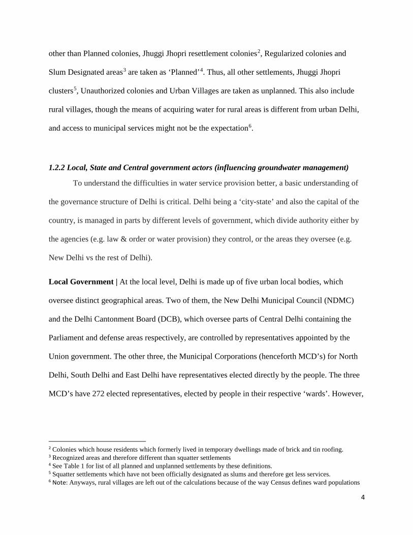
other than Planned colonies, Jhuggi Jhopri resettlement colonies2, Regularized colonies and
Slum Designated areas3 are taken as ‘Planned’4. Thus, all other settlements, Jhuggi Jhopri
clusters5, Unauthorized colonies and Urban Villages are taken as unplanned. This also include
rural villages, though the means of acquiring water for rural areas is different from urban Delhi,
and access to municipal services might not be the expectation6.
1.2.2 Local, State and Central government actors (influencing groundwater management)
To understand the difficulties in water service provision better, a basic understanding of
the governance structure of Delhi is critical. Delhi being a ‘city-state’ and also the capital of the
country, is managed in parts by different levels of government, which divide authority either by
the agencies (e.g. law & order or water provision) they control, or the areas they oversee (e.g.
New Delhi vs the rest of Delhi).
Local Government | At the local level, Delhi is made up of five urban local bodies, which
oversee distinct geographical areas. Two of them, the New Delhi Municipal Council (NDMC)
and the Delhi Cantonment Board (DCB), which oversee parts of Central Delhi containing the
Parliament and defense areas respectively, are controlled by representatives appointed by the
Union government. The other three, the Municipal Corporations (henceforth MCD’s) for North
Delhi, South Delhi and East Delhi have representatives elected directly by the people. The three
MCD’s have 272 elected representatives, elected by people in their respective ‘wards’. However,
2 Colonies which house residents which formerly lived in temporary dwellings made of brick and tin roofing. 3 Recognized areas and therefore different than squatter settlements 4 See Table 1 for list of all planned and unplanned settlements by these definitions. 5 Squatter settlements which have not been officially designated as slums and therefore get less services. 6 Note: Anyways, rural villages are left out of the calculations because of the way Census defines ward populations

5
all the five bodies virtually are accountable to the Union government and are headed by
Commissioners appointed directly by Ministry of Home Affairs.
State government | Like any other state in India, it has a state parliament, which manages
transport, industrial development, revenue administration, power generation, food and civil
supplies and health and family welfare. However, because it is the capital region, unlike other
states, the responsibility of any physical planning as well as that of law and order is assumed by
the union government itself.
Union government | The central government, (or the federal government as in the US), Union
government reserves some important functions in the state concerned with security and physical
planning as seen in Table 2.
Table 2: Governance structure for various Urban Services in Delhi
Level of government Authorities/Bodies Union Ministry of Home Affairs | Delhi Police
Ministry of Defense Ministry of Urban Development | Delhi Development Authority
State Delhi Jal Board (DJB) Urban Development Department (UDD) Delhi Urban Shelter Improvement Board (DUSIB) Six companies for electricity generation, transmission, and distribution
Local New Delhi Municipal Council (NDMC) Delhi Cantonment Board (DCB) Municipal Corporations of Delhi (North, South, and East)
Difficulties form a 3-tier governance structure in water provision: Thus, Delhi remains a
governance structure often called that of "limited statehood" (Center for Policy Research, 2015).
Politicians often attribute failures of governance to the complexities arising due to such structure
of shared responsibilities and thus shared accountabilities between the three tiers of government.

6
As we would see later, while the responsibility of water service lies with the Delhi Jal
Board (DJB, see above figure), which is directly controlled by the state, the accessibility of water
services depends on the legal status of a household. The power to certify which lies with ( ), an
agency controlled by the Union government. Also, while the Delhi Development Authority
(DDA, a union agency) is responsible for development of land and housing in Delhi i.e.
development of planned settlements, the state only oversees Delhi Urban Shelter Improvement
Board, which is responsible for slum rehabilitation, i.e. the upkeep and care of informal (and thus
naturally unplanned) settlements. Thus, while the degree of accessibility to water services
provided by the state depends majorly on planned-ness of settlements, the state has no power to
direct growth of planned settlements itself.
1.2.3 Delhi Jal Board
The central actor in this study is the Delhi Jal Board (Jal = Water) or DJB, is state
institution which oversees water provision as well as groundwater management. DJB in its
current form was constituted by the DJB Act of 1998. DJB manages water and sewage related
infrastructure in 95% land area of the state, except in the areas of the urban local bodies, NDMC
and DCB, which are directly controlled by Union government elected representatives.
The DJB, being a state institution, gets most of its income from state government grants.
CPR report also notes that the DJB receives a bigger share of state funds than even the three
MCD’s combined. Though its funds are heavily skewed towards sewerage, where it allocates
more than 70% of its budget in 2012-13, while water supply got less than 30% of the funds.
The DJB’s governing board has representatives from all three tiers of government, as
well as representatives from the Central Ground Water Board (CGWB), which is another

7
important actor in this research. We’ll stress this role of CGWB as a representative on DJB board
in next section.

8
Part 2: Understanding policy context
Groundwater use for domestic or other purposes is considered to be a significant factor
which causes the water table depletion in Delhi. In a metropolis of the scale of Delhi, it is
unusual and understandably unsustainable for people to depend on groundwater rather than
municipal provided water or purified water from other sources. One of the direct reasons is lack
of piped water supply. But previous researches and policy studies have identified reasons beyond
that, which result in groundwater dependence, such as Delhi Jal (Water) Board’s policies and
issues of erratic water supply.
2.1 Review of DJB’s policies
The DJB Act of 1998, which constituted the Board, also defined its roles, responsibilities
and even where it’s mandatory or not to provide services. Several authors have pointed out this
caveat in the foundational legislation of the Act, which goes like this:
“..this clause shall not be construed to require the board to do anything which is not in the opinion of the Board practicable at a reasonable cost, or to provide water supply to any premises which have been constructed in contravention of any law or in which adequate arrangement for internal water supply, including internal storage, as may be required by the Board, does not exist.”
Thus, DJB is not ‘obligated’ to provide services in ‘unplanned’ settlements. (CPR 2015).
However, this doesn’t stop the Board from extending its services to unplanned or illegal
settlements, the only consideration being whether it is ‘practical’ to do so. The guarantee of
tenure is an important consideration for defining practicality, which again points towards the
difficulties of service extension to transient settlements. CPR reports through a senior
One salient feature to note here is that, DJB often states the improvement in access to
services in terms of increase in the length of infrastructure, and not by number of people served
or left out of the system. This method of evaluation is understandably flawed, as the Delhi

9
Development Report (2013) demonstrated, that even though the piped water supply increased in
coverage from 75% to 81%, access to water in unauthorized colonies and JJCs remained largely
“unsatisfactory”.
Table 3: Access to 'individual' piped water connection in different settlements. Source: (Maria, 2008)
Though the access to water is not only through piped water. Both DJB and the residents
themselves make alternate arrangements to the formal network supply. Two methods being the
most prominent, water distribution through water tankers and procurement through bore wells.
Both means of procuring have had serious implications on ground water levels. It is important to
note here that DJB itself relies on ground water as a water source, though it accounts for only
about 8% of the total supplied water as per their estimates. The criticality of ground water was
even realized by the 1998 Act, which states that the second role of DJB would be to:
7 Jain (1990) 8 (Suparna Singh, 2018)
Classification as per this study
Settlement Types (Classification generally followed)
Tenure Poverty7 Access to individual tap connections
Planned Settlements (73.5% of Delhi’s population)
Planned Colonies Legal Low Good situation Slum Designated Areas
Legal Mixed Restricted by technical features
JJ Resettlements Colonies
Legal High Official right not respected
Regularized-Unauthorized colonies
Legal Mixed Good situation
Rural Villages Legal Low Not under the responsibility of the DJB Unplanned settlements (26.5% of Delhi’s population)
JJ Clusters Illegal High No right to individual connection Unauthorized colonies Semi Legal Mixed No right to individual connection Urban Villages Legal Mixed Good situation, but part of supply may
be through groundwater sources8

10
“plan for, regulate and manage the exploitation of ground water in Delhi in consultation with
Central Ground Water Authority and also give advice in this regard to... local authorities, except
with the prior approval of the central government.”
2.2 Issues of supply in absence of piped water
A) Supply through Water Tankers
The water tankers are an alternative arrangement done by DJB, to supply potable water in
water deficit areas. Water deficit areas are either the ones which have no piped water supply or
ones which have limited supply inadequate to meet demand, especially during summer months.
The tanker system uses two types of tankers, one provided by the Board and other private
tankers contracted out by the DJB, which are slowly phased out of the system. However, both of
these have certain issues. The private systems had been accused in the past of filling these
tankers with unregulated ground water, resulting in a decision by the National Green Tribunal in
2013, which mandated all tankers operating within Delhi to get registered with DJB.
DJB’s own tanker system has faults. DJB employs two types of tankers, the old ones called as
‘department tankers’, and the new fleet ‘GPS enabled Stainless steel tankers. The departmental
tankers had long been accused of deviating from routes and selling the water to private suppliers
which in turn sell the water for a profit. These tankers also are infamous amongst the residents
from their poor water quality.
While the GPS enabled new tanker, fleet improved over these shortcomings of black
marketing of water, they are not independent of accusations of bias in service provisions. The
tankers though have designated stops, these distribution points cannot be believed to provide an
equitable distribution of water. Tankers are often at the helm of influential persons or those with

11
political connections, which decide the stop point for the tankers, leading to a distrust for the
service (CPR, 2015). While the DJB aims for greater transparency and customer satisfaction for
tanker service, through publishing tanker schedules online and running a call center for
complaint addressal, the residents largely remain unaware of tit, or cannot access them due to
digital divide. The issue of poor quality persists, while some residents are deterred by the long
queues, and thus some residents refuse to collect water provided by DJB tankers.
B) Supply through Tube Wells
The DJB also operate tube wells which are monitored for quality across such settlements
which are known to face water shortages or do not have access to piped water. However, such
tubewells comprise of a tiny percentage of actual number of illegal tubewells operating across
Delhi (NGT, n.d.)

12
Part 3: Literature Review
This section looks at the existing literature about water access and usage in Delhi, to
explore reasons further than the policy and supply side problems identified in the previous
chapters. Case studies by researchers and anthropologists identify various issues at the consumer
end such as affordability, insecure tenure and dissatisfaction with community sources of water
also contribute to groundwater usage by the residents. Lastly, this section looks at empirical
studies, both from government organizations and researchers around the world, to learn identify
key variables, scale and methods of analysis.
3.1 Review of consumer-side factors leading to groundwater usage:
Inequities in access to piped water: While the planned areas, urban villages and regularized
colonies are believed to have the good level of water service (Maria 2008), the above-mentioned
systems of differentiated citizenships engrained in the DJB Act result in different levels of access
to water for each type of settlement.
As aggregate Census numbers do not differentiate between these different types of
settlements, they do not tell the whole story of access to water. Adding to this, the estimates of
supply variability between different settlements are difficult to obtain from DJB’s own data. The
water supply tables published by DJB, state demand and supply volumes at a very macro scale
(in DJB revenue zones) (GNCT Delhi, 2017).
Multitude of field studies by local universities and anthropologists (Safe Water Network,
2016, Roy, 2013, Grönwall, 2011), as well as government’s own reports (Srivastav P.P, 2007)
make these differences in the provision of municipal services clear. Service provision often vary

13
within the same settlements, for e.g. only the houses which face the main road have been
connected to piped supply. In the case of Jaffrabad, a large 40-year-old colony in Delhi, this
forces residents to rely on private borewells. (Safe Water Network, 2016). In some cases, even
the piped connections run dry, and great distances to communal treated tap water sources, forces
residents to opt for hard water from nearby bore-wells, which they boil and use (Roy, 2013).
Affordability issues, barriers due to price of connection: Many HHs even after getting the
option of piped water access, decide not to apply for a connection given the high cost.
Acknowledging the high pricing of fixed connections act as barrier to get formal connections, the
government has recently tried to lower to include more people into the piped network of the city.
(Suparna Singh 2019).
However, illegal access to water also poses a financial cost, particularly on the slum HHs.
Case studies report about 63% of HHs pay an initial cost to gain access to water, which includes
bore-well construction costs and cost of submersible pumps amongst other things (Safe Water
Network, 2016). The costs increase with greater depths of groundwater. However, even if high
groundwater levels lower the cost of installations, such groundwater could be of lower quality,
and thus pose public health issues. (Gupta & Sarma, 2016)
To be reminded, DJB does provide alternate means to access water in the absence of
piped connections, or in case of insufficient supply, in form of tanker water or communal taps.
Discontent due to sharing and distrust over water quality: Though even these HHs which have
access to these alternate means, might not end up using these sources. As community taps are
shared between 10 to 30 HHs, and majority residents spend 30-60 minutes daily to fetch water,
this deters residents from these services by DJB. (Safe Water Network, 2016).

14
Slums, while being legal settlements, rely on such community taps for water
requirements. Table 2 above shows this is due to technical difficulties in laying pipes through
winding streets and complex built forms. This fact is further confirmed by Census 2011. Only
51% of slum HHs have water source in premises, while the statewide average is 78% of total
settlements. This points that even between all settlements classified as planned in this study,
there exists different levels of water access.
Lack of potable water in absence of piped supply, is further aggravated through a general
distrust and the high costs of tanker water. As a result, it is ‘quite common’ for to people opt for
secondary sources, like tube-wells and bore-wells, though for non-potable use (Safe Water
Network, 2016).
Figure 2: Pic: Waiting in queue is the norm to get water from tankers. Source: (Singh, 2017)

15
Impacts of Insecurity of tenure on dependence on groundwater: While the unplanned
settlements make constant efforts to improve access to municipal services, the label of illegality
could also lead to a ‘passive acceptance of ecological problems. The HHs in such settlements,
who are tenure insecure, especially in JJ clusters, use “threat to transient existence” as an excuse
to avoid demanding water related services in the locality. (Roy 2013) The insecurity of tenure
also prohibits these HHs to pool in time and resources to make permanent or at least safe
arrangements for water access. However, they still make individual arrangements through private
tube-well operators who install private pipelines.
The restriction to access piped water are also sometimes perpetuated by government own
rules. Until 2015, government restricted number of connections to a single building at 6, while
Figure 3: Access to water in Slum households in comparison to all households. Source: Census, 2011

16
other renters/owners were required to arrange for their water through underground tanks, thus
leaving out people who had access to tap water, both physically and financially (PTI, 2015).
Groundwater dependence for sustained water security: However, the distinction between
planned and unplanned settlements is often rendered meaningless, as even the now regularized
colonies which get piped water supply, continue to use borewells. Water from borewells acts as
free and reliable source of water in comparison to irregular municipal supplies. (Truelove 2007).
In addition, richer households often use tube wells, which have a high initial cost but provide a
free and reliable service thereafter to counter erratic municipal water supplies, especially in the
summer months. Moreover, tube-wells arguably also provide the luxury of avoiding the hassle of
obtaining water within specific times, as majority of colonies in Delhi receive water for about
couple of hours in the day (Rounak Kumar Gunjan, 2020).
Thus, tubewells remain a major primary or alternate source, used to satisfy potable and
non-potable water needs. To be sure, even Delhi Jal Board uses groundwater along with regular
treated water, to supply urban villages which were newly connected to the city system. (Suparna
Singh 2019) But there is general acknowledgement that the DJB tubewells form a miniscule
percentage of the actual number of tubewells operating in the city, majority of them illegally.
CGWB and DJB have taken many measures over time in order to restrict use of illegal tube
wells or to regularize them. The CGWB in 2010, mandated that every tube well operating in the
state should take prior permission from the DJB or NDMC. Further, in 2012 they decided on the
following criteria for obtaining such permission:
17
1. There must be no public water supply system in the area. 2. The applicant must have a certificate from the water supply agency stating that the there is no such supply
in the area. 3. The applicant household cannot already have a tube well or bore well.
It is clear from the requirements that it was an effort to document the new bore wells, not
directed towards enumerating the already operating ones. In addition, a lot of tube wells as seen
from numerous case studies operate in areas with a formal piped water supply, but which is
inadequate. Tube well water is not used as potable but for other needs. Also, the lengthy and
complicated process of obtaining a permission, might have deterred the applicants as only 976
tube wells were registered with the DJB as of 2014. These was also an opportunity lost in regard
to any attempt of enumerating tube wells. CPR report noted that their fieldwork suggests that
given the complicated nature of the process, far less tube wells have been registered, rendering
majority of them illegal.
DJB in early 2014, made task force to identify and regularize the in-use tube wells in
unplanned settlements. The few tube wells that were overtaken by DJB, were handed over to
Resident Welfare Associations, and the neighbors started getting their water at one tenth of the
prices they paid to private operators. Thus, after a tube well is regulated, the price goes down for
the residents, but this does not have impacts either on the quality nor on the quantity of
groundwater exploited.
Complementing these actions by DJB, the LG released a notice asking operators and
residents to voluntarily disclose their tube wells. However, the uncertainty regarding the future
actions, again discouraged most from doing so, and again an opportunity was lost to identify the
actual scale of these illegal operations.

18
Thus, there is no reliable estimate for the number of tube wells, which operate outside the
knowledge of the DJB, adding to which the previous efforts of estimating their number has been
nullified by complicated and unclear policies.
However, as we see in the next chapter, enumerations of tube wells are generally not used in
groundwater draft calculations. It is thus important to next review what are the current methods
of estimation, and the factors identified by both the public authorities and scholars impacting
groundwater levels.
3.2 Review of groundwater studies
3.2.1 CGWB methods and policies
The Central Groundwater Board is the authority which carries out annual review of
groundwater levels in Delhi, and publishes data about the current level of exploitation and future
potential of the use of groundwater for irrigation, domestic or industrial use, which has informed
the Water Policy of 2016 and the recent Summer Action Plan, constituted in 2019 in the city.
The handbooks use two ‘correlated’ factors to decide groundwater potential, verifying results of
one factor with the other.
• The trend of groundwater changes over 10 years
• ‘Stage of groundwater development’9
Stage of groundwater development is basically dependent on three factors, the groundwater
availability in a region, the annual recharge from rainfall and other sources and the
groundwater ‘draft’.
9 The term Groundwater Extraction was replaced with Groundwater development, as per recommendations of GEC 2015 report

19
To calculate groundwater ‘draft’ which this study is interested in, the CGWB handbooks
refer to Groundwater Estimation Committee reports, which establish the measures to estimate the
groundwater draft in urban and rural areas since 1984.
The latest GEC report specifies two different methods for estimation of groundwater draft for
domestic use, which are outlined below. (GEC, 2017)
• Unit draft method: This is same as methods used to determine the draft for irrigation. Here, unit
draft for each type of well is multiplied by the number of wells used for domestic purposes.
• Consumptive Use method: Population is multiplied with per capita consumption usually
expressed in liter per capita per day (lpcd).
Understandably, the unit draft method is less suitable for a metropolis like Delhi, as
previously mentioned, there is no reliable estimate for number of wells operating in the city, and
most of them operate illegally. Thus, consumptive use method is more suitable.
However, the reports offer little discussion over how this fractional load is calculated.
The general method to calculate fractional load is to calculate the difference in municipal supply
for the area and per capita need of water.
3.2.2 Groundwater studies and methodology
Sampling and interpolations: To study how groundwater varies in a region or a city, either in
terms of water tables or quality of water, sampling and analysis may be done in various ways.
Water levels can be obtained from yearly reports from Central Groundwater Board, a central
20
government institution, tasked with monitoring groundwater usage. For a region wide analysis,
all available data points from the CGWB reports may be used (Dash, Sarangi, and Singh 2010),
or aggregation of observed values could be done to perform a region-based analysis instead
(Chatterjee et al. 2009).
Individual sample points or a strategic sampling of available well values, could help in
studies with a special purpose, for e.g., difference in groundwater depletion between agriculture
land and urbanized land (Trivedi et al. 2001), or between different land covers like forests, parks
and settlement areas (Gupta and Sharma 2016). The unit of observation vary from administrative
units comprising of a population of a million (Dash et.al 2010), to small villages with a
population of a few thousands (Trivedi et al. 2001).
Similarly, to extend analysis over a larger area once the samples are collected, the
methods for interpolating water levels can employ variety of methods, however two of them,
namely Inverse Distance Weighting (IDW) (Taleb Odeh 2019) and Krigid (Dash et.al 2010) find
most mention. Both methods are primarily based on Tobler’s Law (Everything is related to
everything else, but near things are more related than distant things). While IDW is advantageous
over normal interpolations as it can account for surface gradient changes, Kriging also considers
the overall spatial arrangement among the measured points in addition, and outputs a measure of
confidence of predictions. Thus, this study will make use of Kriging to interpolate groundwater
levels.
Important Factors influencing groundwater change: Like CGWB studies, contemporary
researches identify rainfall variations as an important factor influencing groundwater levels,

21
other than anthropogenic factors (Okkonen & Kløve, 2010 ,Hu et al., 2019,). Also, for studies
focusing on impacts of city growth through study of land cover and groundwater withdrawal,
rainfall variations form an important control variable (Choi et al., 2012).
Another factor of importance in groundwater studies, especially for studies tracking
impact of urbanization over groundwater over time, is the land cover change. While land–cover
changes are generally used as a measure of growth of the city, in terms of demand for water, it is
also an important factor influencing storm water runoff and rainfall permeability. In fact, some
studies identify land-cover as a factor of influence even for micro-level changes in rainfall,
which is an important factor in CGWB studies to estimate future availability (Kharol et al., 2013,
Cao et al., 2015). While most studies use remote-sensing to observe variation in land-cover/land-
use over time, their classifications of land-use vary according to perceived factors influencing
groundwater change for e.g. binary classification as urban and agricultural land cover in dry
areas (Odeh et al., 2019) or multiple classes which also account for water bodies in tropical
climates (Patra et al., 2018). However, the calculation of urban land cover in most studies
reviewed is based on surfaces covered by impervious surfaces such as asphalt and concrete (or
paved and concrete surfaces) (Tam & Nga, 2018).
Other than remote-sensing studies, urbanization studies also account for the impact of
population or population density as an important factor contributing to change in quantity or
quality of groundwater.
Methods of analysis: correlation studies, GWR, map overlay.
Most of the above studies, use correlation analysis, either through specific software’s or
studies observing land cover change as single factors, also employ map overlay analysis

22
GWR is a recent technique which finds applications in several groundwater studies. GWR is
particularly useful if the dependent variables are available in point formats.
Learnings from methodology studies
From the studies reviewed above, some of the factors that this study should include should be:
• Ways of estimating changes in groundwater levels • Estimate of rainfall variation • Dependence on land cover and population
Need of a new definition
It could be observed from the studies above that though the current methods of estimation
specify broader methods of estimation treating population and built form uniformly, the case
studies visited in previous section, explain that the patterns of dependence on groundwater are
not uniform over the entire urban population. Even in areas which receive municipal supply
depend on various factors such as price of water connection, trust over quality of water and
affordability of supplementary borewell connection. For example, the CGWB report estimates
following domestic draft for two Tehsils in Delhi:
Table 4: Population and domestic draft for two sub-districts of Delhi
Sub districts/Tehsils Population (as per Census 2011)
Domestic draft (as per CGWB Handbook 2015)
Vivek Vihar 247906 403.68 Preet Vihar 1062568 813.43
Not only the population groups are different, but the difference in settlements is also seen
in the variables of ground cover and built form. The following picture exemplifies this
difference. On the left side is Khichripur urban village, and adjacent to it is the Kalyan Puri
Resettlement Colony, which is planned and constructed by DSUIB. This satellite image clearly

23
shows the difference of physical forms between planned and unplanned settlements. The
resettlement colony on the right has neatly lined streets with trees, and green, open spaces which
allow groundwater recharge. While the urban village is a dense built form with little tree cover
and open spaces. Therefore, a distinction which could be missed by the above-mentioned
groundwater researches correlating land covers, through remote sensing.
Figure 4: Difference in land cover between Khichripur Urban Village (unplanned settlement) vs. Kalyan Puri Resettlement Colony (planned settlement). Source: Google maps
Thus, there needs to be a new way to estimate groundwater draft which accounts for such
differences between population groups and type of settlements, based on all these factors.
Learnings from this literature review inform our selection of variables in the next section.

24
Part 4: Research Methodology
4.1 Defining variables
Independent variables:
Drawing from research studies on Correlation analysis:
• Variable to control for variation in rainfall and physical factors o Total groundwater recharge
• Variables to control for built form and land cover variation o HHs having concrete roofs
Drawing from research studies on groundwater dependence in Delhi:
Lack of piped water supply:
• Variable defining access to piped water o Percent HHs having access to treated tap water:
• Variable to distinguish the unit of analysis as planned/unplanned o Percent HHs in Unplanned settlements
Demand side factors:
• Variable defining the use of tube wells o Percent HHs identifying tube-wells as the primary source of water
• Variable defining community/individual sources of access o Percent HHs having a primary source of water within premises
• Variable defining socio-economic status of HHs o Percent HHs owning a Car
• Variables defining security of tenure o Percent HHs owning the house
Data collection and manipulations
Table 5: Selected Independent variables and their source, time and scale of available data.
Variable Source Time over which data collected
Scale Measurement Unit
Recharge Aquifer Mapping and Groundwater Management Plan
2013 Sub-district Ham (hectare-meter)

25
Variable Source Time over which data collected
Scale Measurement Unit
Roof_Concrete H-14, Houselisting and Housing Census
2011 Ward Number and % of HH
Tap_Treated -same- 2011 Ward -same- Plan Slums |DUSIB JJ
enumeration 2015-16 Assembly
Constituency -same-
Unauthorized Colonies | Scraped from RWA regularization applications
2018-19 Assembly Constituency
-same-
Urban Villages | Revenue Department Notification List, Manually Geocoded
Compiled 2013/ Last Revision 2002
Point data -same-
Tubewell H-14, Houselisitng and Housing Census, 2011
2011 Ward -same-
Within_premises -same- 2011 Ward -same- Car_Jeep_Van -same- 2011 Ward -same- Owned -same- 2011 Ward -same-
4.2 Selecting Unit of Analysis
The state of Delhi is can be divided based on two type of units, first being political,
deliberations for which are
decided by ECI, and second
being the unit of analyses used
by Census and various Central
government agencies.
Political units:
Municipal wards | Wards are
both political as well as Census
units. (though might not be
large enough to account for Figure 5: 272 wards of Delhi

26
variation in groundwater levels. Moreover, the unplanned settlements are available by AC no.
and disaggregating these to smaller units at ward levels might render the data highly inaccurate)
Assembly constituencies | Like PCs, boundaries were delineated such that each PC, by census
2001, accounted for 200,000 people. At the state level, Delhi has 70 Members of Legislative
Assembly, each representing an ‘Assembly Constituency’ (henceforth AC). Each AC is
delimited based on 2001 Census data, to contain about 200,000 voters.
Parliamentary constituencies | The boundaries were delineated such that each PC, by census
2001, accounted for 200,000 people. Other than 272 representatives at the local government level
and 70 in the state parliament, the people of Delhi are also represented by 7 Members of
Parliament, elected from their Parliament Constituencies (henceforth PC’s). Each PC is delimited
based on Census 2001 data, so as to contain 2 million voters.
Figure 6: 72 Assembly Constituencies of Delhi

27
Census units:
Districts | Districts are the first
divisions into which Delhi is
divided. There were 9 districts in
2011 which have since 2015, re-
divided into 11 districts. Analysis
at a district scale is suitable for
regional studies, and thus not
suitable for our purposes.
Subdistrict or Tehsils | Districts
are further divided at the subdistrict scales. Analysis for groundwater is done by the CGWB at
this level. Also, the rainfall data is available at this scale. Delhi had 27 districts in 2011, and thus
sub-districts, though helpful for accuracy of data (no aggregations required) would provide a
small DOF, not preferable for OLS and more so, not for local regressions.
Choosing the unit: ACs are most suitable unit for this study, as:
Useful scale and sample size: The units are large enough to represent variations in groundwater
levels. Though the CGWB uses its smallest unit as the sub districts or tehsils of Delhi, there are
some limitations: first being the coarseness of variation which might render any analysis or
interpretation useless. Second, being the heterogeneity in each tehsil in terms of natural features,
built features and demographics. As observed from the map, tehsils show close to radial pattern,
thus originating at New Delhi and extending to the boundaries. For e.g., the West district, xy
Figure 7: 9 Districts of Delhi as per old classification

28
subdistrict. Also, 70 ACs form a large enough sample size for regression analysis compared to
27 sub-districts.
Limited variability in population: As population is a defining factor for groundwater studies, the
ACs are an ideal unit of analysis, as each AC had a population of 200,000 in 2001, which can be
assumed to grow at a similar rate across Delhi.
Units of Action: ACs are units which are represented by elected members at the state level. As
mentioned in previous chapters, DJB is the primary body handling all water supply and
groundwater management related works in the state.
More importantly, selecting a political boundary, would ensure the results and suggestions can
be incorporated in decision making, as the revenue districts of DJB overlap with the AC's and
also the action plans are made consulting the local area representatives.
Delineation has remained constant: While the Census data for the subdistricts and wards is
available for the year 2011, the delineations of both have changed since 2015 and 2018.
4.3 Selecting a time frame for analysis
Since most of data sources, record data around 2011, this is an appropriate scale of
analysis (see Table 6). However, the CGWB identifies a 10-year scale as a criterion to observe
long-term groundwater fluctuations. Therefore, in preparation of the dependent variable, a
timeline equally distributed around the year 2011 is useful. 2006-16 is thus a suitable period to
observe change in groundwater levels, assuming that the trend was similar in 2011.

29
4.4 Data preparation
A) Dependent variable:
The reference data for groundwater level
change for 2006-16, is the map of decadal
water level fluctuations, printed in 2016
Groundwater Yearbook of Delhi, produced
by CGWB. Two methods were tried, firstly,
to reproduce this map, and secondly,
digitizing the raster map with published
ranges to calculate groundwater level change
within each AC.
Results of Kriging:
Groundwater level for each well was
extracted from the Water Resources of India portal. Since the reference map uses, Post-Kharif
values as observations, the Kriging was performed over these values.
On the left is the raster obtained after subtraction of mean well values over the decade
and those in 2016. As can be observed, the raster reproduces the reference map accurately in all
places, except in Southern parts of Delhi, which are masked by a Ridge, and also has different
elevations than rest of the state.
Figure 8: Decadal fluctuation in Groundwater levels between 2006-16. Source: CGWB Report, 2017
30
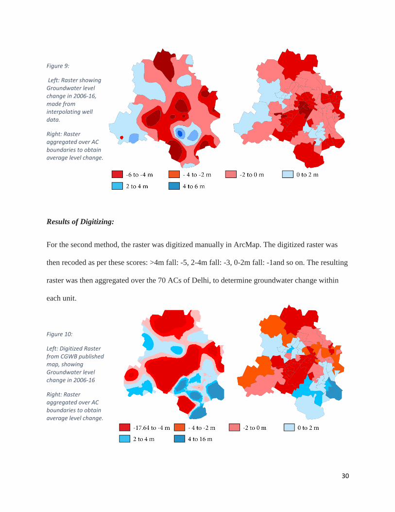
Results of Digitizing:
For the second method, the raster was digitized manually in ArcMap. The digitized raster was
then recoded as per these scores: >4m fall: -5, 2-4m fall: -3, 0-2m fall: -1and so on. The resulting
raster was then aggregated over the 70 ACs of Delhi, to determine groundwater change within
each unit.
Figure 9:
Left: Raster showing Groundwater level change in 2006-16, made from interpolating well data.
Right: Raster aggregated over AC boundaries to obtain average level change.
Figure 10:
Left: Digitized Raster from CGWB published map, showing Groundwater level change in 2006-16
Right: Raster aggregated over AC boundaries to obtain average level change.

31
Choice of values: The results of interpolation mirror the reference map correctly, expect for
Southern parts. These parts have been constantly mentioned as critical, in many CGWB reports
over the past decade, and thus form an important part of this study. Therefore, the latter derived
values of dependent variables are more suitable and reliable for the purpose of this study.
However as mentioned previously, the values are only as informative as the raster at the scale of
digitization, and thus, though the Y values are continuous, they show limited variation, only from
–5 to +5 m. In reality, the variation is much larger, as observed from the values of Kriging
interpolation. Therefore, the Y values can be considered as ‘Scores’ rather than absolute values
of groundwater change.
B) Independent variables:
Most of the independent variables are directly taken from Census 2011 data or from CGWB
studies (see Table 6). The interaction term, however, has to calculated as no official data exists
as per the definitions of this study.
Interaction term | The interaction term which would distinguish between planned and unplanned
settlements is prepared as follows: First, the number of populations in different types of
unplanned settlements of Delhi as this study classifies them, are identified. Then, these are
aggregated and the percentage of HHs in unplanned settlements over total number of HHs in an
AC is determined. A threshold percentage is specified, based on which an AC is classified as
planned or unplanned.
Slum HHs: DSUIB published an Assembly Constituency wise list of 675 slum HHs with
population, no. of households.
Unauthorized colonies: As previously mentioned, the State government and central government
had been proactive in regularizing the UCs before 2020 elections. For this each UC had to

32
constitute a Resident Welfare Association, which then furnished list of documents before the
state government. An example of such documents is shown in the left side10. The red rectangle
highlights the plot count and approximate population of the colony mentioned in each form, This
data was manually entered and aggregated to count total HHs in such colonies in each AC.
Figure 11: Left: A sample application form filed by RWAs for regularization. Right: Official List of 1731 Unauthorized colonies with AC numbers.
Urban Villages: No comprehensive list exists to indicate the location of the UVs. While the
revenue departments have estimates of the number of HHs, the boundaries of these remain
arbitrary. Thus, the following workaround was adopted: 1) Each UV was geocoded by manually
10 Note: a basic analysis of the scraped data reveals that there are differences in terms of the household sizes. This could be explained by another form in the set, which asks whether the households own the land. Thus, while the UC through the case studies reveal presence of renters, some forms might not have counted them in the population as is not required by the application process. Thus, it is expected that the actual number of HHs are greater than those listed, if the renter HHs are counted for all colonies.

33
searching by name. However, the urban villages cannot just be aggregated as point features, as
many of them lie at an intersection of many Assembly Constituency. Therefore, to minimize
error in counts while aggregating the village population to respective AC’s, each point was
assumed as the centroid, which was then transformed into circles by spreading the population as
per average density of an unauthorized colony in Delhi11. These circles were then aggregated on
to AC boundaries to find the number of households in each. For e.g.,
For the village of Rithala: Population: 4,047
Assumed population density: 8,254 people/sq. km (Population density of North-West District)
Estimated buffer: a radius of 390 sq. m
11 Average HH size: 4.7. Average population density 11,320 persons/sqkm (as per Unauthorized Colony data)
Figure 12: Satellite View of Rithala Urban Village

34
Classification as Planned/Unplanned:
Adding all HHs count calculated above for each of the AC, and then determining the
share of unplanned over total HHs in an AC, the mean percentage of unplanned HHs was found
to be around 30%, the median being around 28%.
Taking a cue from the numbers, two thresholds for this study were tried, at 25% and
40%. The maps below show the distribution: Taking a cue from the maps and counts12, the
threshold for this study will be assumed at 40%. A 40% threshold shows a more regular
distinction and overlaps accurately with the actual built form of Delhi13. Therefore, ACs with the
ratio of less than 40% of unplanned HHs to total HHs will be counted as planned. 48 ACs were
counted as planned and 22 as unplanned by this definition14. The map below shows the
distribution:
A broad distinction between the two kind of areas can be seen here15. The blues cover
most of the central part of Delhi, which has the Parliament, important institutions and the
12 For a threshold of 25%, 35 ACs are classified as planned and unplanned. 13 such as classifying the AC’s having DDA colonies in East Delhi correctly as planned 14 Population of ACs overlapping two Sub-districts, Narela and Najafgarh was modified by the factor of (Total Population/Urban Population) to account for total number of HHs, both rural and urban. Rural HHs are not counted for ward level data and thus were not aggregated in AC popualtion. 15 Variables taking this distinct spatial structures can be employed too, for e.g. dummy variables for central and peri-urban/rural areas.
Figure 13: Summary statistics of share of HHs living in unplanned settlements in each AC

35
colonial parts of Delhi. The Reds form a radial ring around these, for these were the parts where
most of the Urban Villages were located before the city expanded.
Figure 14:Blue units as Planned ACs and Reds as unplanned ACs of Delhi

36
Part 5: Analysis
5.1 Correlations
A basic correlation analysis for all the selected variables reveal expected relationships
amongst the variables. The above correlation matrix shows the scatterplot on the left side and the
R-values to the right of all variables. Values with high correlations suggest that the variables
move together in same or opposite directions, and therefore the relationships between any such
variables are like its correlated dependent variable.
Figure 15: Correlation matrix and Scatterplot matrix for all variables (dependent and independent)

37
As a rule of thumb, variables with R-value of around 0.7 or above are generally treated to
reduce redundancy and to specify the model correctly. Following treatments are made to limit
multi-collinearity:
Table 6: Treatment for variables with high correlations
Variable High Correlations with
Inference Treatment
ROOF_ CONCRETE
+ with Tap_Treated + with Within_Premises + with Car_Jeep_Van
The HHs having a concrete roof overhead, expectedly also get piped water supply, in their premises. Also, ACs with higher % of such HHs also have wealthier HHs and thus more share of HHs owning a four-wheeler. The relationships are all indicative of populations in planned settlements and their collinearity is expected.
The variable is to account for land-cover, a determinant of ground permeability for groundwater recharge. As it is accounted by variable RECHARGE, this variable can be dropped form the equation.
TAP_ TREATED
- with Tubewell + with Within_Premises
ACs with higher % of HH with a municipal water connection, naturally have lower share of HHs owning a tube well. The correlations also suggest that such HHs generally have connections in the premises i.e. piped connections are more through private than communal taps.
The variable forms an important factor for this study, and therefore cannot be omitted. Moreover, the variables are correlated, but not explain each other completely. E.g. a HH can access treated water from a source outside its premises and is more likely to use borewell as an alternate source according to case studies. To preserve the variable and decrease the collinearity, a new variable is specified: Treat_by_Tube = Tap_Treated / Tubewell
The revised correlation matrix with the final selection of independent variables is shown below.

38
The scatterplots above point towards a near linear relationship between all selected
independent variables and the dependent variable. The following are descriptive statistics about
each variable for planned and unplanned settlements.
Table 7: Range and distribution of each independent variable
Variables Unit Planned AC’s Unplanned AC’s Min Median Max Min Median Max
Owned % HH 23.70 69.04 78.57 48.21 71.03 79.66 Treat_by_Tube Ratio/unitless 0.37 49.82 826.16 0.84 5.03 1327.52 Within_premises % HH 50.85 84.30 95.28 22.47 70.62 93.99 FWheeler % HH 4.14 23.72 52.33 3.99 15.24 50.45 Recharge Hectare-m 47.37 188.90 957.53 21.93 416.71 3872.14
Figure 16: Correlation matrix and Scatterplot matrix for modified variables

39
5.2 OLS OLS regression is arguably the most used form of correlation analysis in social sciences. A
simple linear model with the general form is:
Y = α + β1x1 + β2x2 +.. βnxn + e
Given this additive, linear structure, it is easy to calculate the expected (i.e., predicted) value of
Y given any values of X:
E[Y] = E[BX + ε] = E[BX] + E[ε] = BX
where E[∙] represents the expected value and E[ε] = 0 by assumption. In other words, the
predicted value of Y is obtained by summing up the BX’s. The residual is the difference between
the actual Y and the predicted value BX. OLS regression takes observations of the X and Y
variables and estimates the B coefficients in equation (1) that minimize the sum of the squared
residuals.
GW_MeanScore ~ β0 + β1Owned + β2 Treat_by_Tube + β3 Within_premises + β4 FWheeler + β5Recharge + e
Since, multicollinearity was an issue with the selected variables, as a matter of standard practice,
VIF or Variance Inflation Factor for the above variables is calculated. Higher values of VIF
indicate the presence of multicollinearity, and a value of 1 indicates a complete absence of it16.
The following table specifies that the model is correctly specified with little correlations amongst
the variables.
Table 8: Variance Inflation factor for independent variables
Variables Owned Treat_by_Tube
Within_premises
FWheeler Recharge
VIF 1.144626
1.339677 1.299220
1.553686 1.032926
16 Generally, a value of 5 or more is considered as a ‘problematic’ amount of multicollinearity (James et al., 2013). ESRI guides recommend a value of 7.5 or lower.

40
Model: As our hypothesis states, because of the physical, socio-economic and service level
differences between planned and unplanned settlements, the relationships between Y and X’s are
different amongst those marked as planned and unplanned. To make this distinction in the model,
we create a dummy variable ‘d’ and code it as 0, if the settlement is planned17, and 1 if the AC is
classified as unplanned. We create an interaction variable for every dependent variable, like:
i.Tubewell = d * Tubewell. Model is thus specified in the form:
Y = α + β1x1 + β2(I*x1) + β3x2 + β4(I*x2) +.. + Βd(d) + Βnxn
The complete equation is thus18:
GW_MeanScore ~ β0 + β1Owned + β2 Treat_by_Tube + β3 Within_premises + β4 FWheeler + β5 Recharge + β6 i.Owned + β7 i.Treat_by_Tube + β8 i.Within_premises + β9 i.FWheeler + β10i.Recharge + β11 d
Results of OLS: Table 9: Results of OLS regression, with coefficient estimates, standard errors and p-values.
GW_ MeanScore19 Predictors Coefficients Standardized
Coefficients Std. Error p
(Intercept) 310 0.00 277.47 0.26 Owned -6.82 -0.43 2.45 0.007 Treat_by_Tube -0.20 -0.23 0.18 0.27 Within_premises -0.37 -0.03 2.53 0.88 FWheeler 2.97 0.22 2.12 0.16 Recharge -0.24 -1.14 0.16 0.13 i.Owned 4.80 0.95 5.78 0.40 i.Treat_by_Tube 0.54 0.53 0.26 0.04 i.Within_premises -4.28 -0.87 3.59 0.23 i.FWheeler -5.46 -0.32 5.40 0.31 i.Recharge 0.33 1.65 0.16 0.04 d -99.17 -0.28 518.03 0.84 Observations 70 R2 / R2 adjusted 0.304 / 0.172 F-statistic: 1.612 on 11 and 58 DF, p-value: 0.02
17 As specified in the previous chapter I.e. ACs with less than 25% of total HHs living in Unplanned settlements (Slums, Urban Villages and Unauthorized colonies) 18 VIF values for the new model with interaction terms is not tested here as it the terms are expected to be correlated with each other, and thus have a higher VIF 19 GW_MeanScore is modified to show groundwater level changes in centimeters instead of meters, for the ease of deciphering regression coefficients.

41
Table 10: Comparison of Coefficients of Planned and Unplanned settlements. Note: the differences are not statistically significant
Predictors Planned AC’s Unplanned AC’s Coefficients Standardized
Coefficients Coefficients Standardized
Coefficients (Intercept) 310 0.00 310 0.00 Owned -6.82 -0.43 -2.02 0.52 Treat_by_Tube -0.20 -0.23 0.34 0.3 Within_premises -0.37 -0.03 -4.65 -0.9 FWheeler 2.97 0.22 -2.49 -0.1 Recharge -0.24 -1.14 0.09 0.51
Evaluating the results against 90% significance, four variables are found significant20. The
low values for goodness of fit (R-square and adjusted R square), devoid the model of any
prediction power. However, the model overall is significant at 90%, and thus could be useful to
observe the relationships between all variables assumed. The key findings about these
relationships are discussed in the next section. However, the model is useful only if the residuals
are not spatially autocorrelated.
5.2.1 Key Findings from the OLS regression
• Variable: Recharge ( Std. Coefficient: -1.14) | However, the standard coefficients suggest that
looking at the impact in terms of standard deviations, i.e. the usual variation in recharge values,
the impact is largest. However, such a large variation is likely to be caused by climate and
hydrological factors rather than by factors under human control such as rainwater harvesting. |
For a per unit change, groundwater recharge has little effect on groundwater levels21
• Variable: Owned (Std. Coefficient: -0.43) | Ownership of the Household has the most negative
effect on the groundwater level change. This suggests a drop-in water levels with rise in
20 The sample size, at 58 DOF is arguably, not large enough to evaluate against the general standard of 95% significance. 21 While contrary to our assumption an increase in groundwater recharge causes a little decrease in levels in planned ACs, while it causes a little rise in unplanned ACs.

42
ownership, instead of a rise which one would normally expect. Since ownership generally grants
access to piped water, results might suggest that tubewell usage which is used as secondary or
supplementary source22 is more frequent, or causes more damage than the tubewell which act as
primary or only source of water. This might also be an indication of a variable closely associated
with house ownership, which impacts water levels, and can be further explored.
Also, note that increase in ownership causes a drop of 3 times of more in planned AC’s
than in unplanned AC’s. For every 10% increase in HHs in planned AC’s, which are owned by
the family living in it, groundwater level goes down by 70 cm, while in unplanned AC’s it falls
by 20 cm. This might suggest that HHs with private tubewell connections cause more damage
than community tubewells, which are more common in unplanned settlements.
• Variable: Treat_by_Tube (Std. Coefficient: -0.23) | The percentage of households using
treated water or not using tube wells as their primary source have a little effect on groundwater
levels. This suggests that expanding the water supply network or access to piped water in itself,
won’t impact groundwater change much. Interestingly, while groundwater levels slightly
decrease with increase in HHs with piped water connections in planned settlements, the levels
slightly rise in unplanned settlements with more HHs connected to water supply network23.
• Variable: FWheeler (Std. Coefficient: 0.22) | Increase in affluence of the HHs within an
Assembly Constituency, causes a rise in water levels in planned ACs, while a fall in water levels
in unplanned ones. For every 10% increase in HHs owning a four-wheeler, the water level rises
by 30 cm in planned ACs, while it falls by similar amounts in unplanned ACs. This might
indicate the rural vs urban nature of unplanned and planned ACs respectively. A variable to
22 Not reported in Census, usually makeshift arrangements 23 However, the relationship as well as the differences are not statistically significant.

43
control for other type of water uses such as for irrigation or industrial use might provide a clearer
picture.
• Variable: Within_premises (Std. Coefficient: -0.03) | With an increase in HHs having sources
of water within premises, the groundwater levels decrease. For every 10% increase in HHs
having their source of water within premises, the water levels fall by about 3 cm in planned
AC’s, while around 40 cm in unplanned AC’s. This is contrary to nature of relationship one
would expect24.
• Variable: d (Std. Coefficient: -0.28) | The result is inconclusive that the relationships between
these factors and groundwater level change, ‘significantly’ differ between planned and
unplanned ACs25. However, the nature and scale of relationships vary between the two on
several parameters.
The results show, hypothesis that groundwater change depends on these factors has some
empirical backing26. The relationships suggest that increasing the piped water supply network
has little effect over groundwater change on its own, while decreasing the price of water
connection might have a greater impact27. Results also suggest that increase in more share of
owners, such as those areas with bungalows rather than rented multi-story apartments, cause a
greater damage to groundwater levels.
Though, only three of these factors are statistically significant, suggesting that the
variables are explaining the same variations and some of these factors can substitute for each
24The large difference in coefficients between planned and unplanned AC’s might point toward a difference in type of groundwater use between urban and rural areas, i.e. for domestic purposes vs for multiple purposes. 25 as the our dummy variable and other interaction variables are statistically insignificant. 26 The model has a p-value of 0.02 which is lower than our expected value of 0.05. 27 If ability to afford a four-wheeler corresponds with that of affordability of a piped water connection.

44
other. For. e.g., a HH owning a car, would be expected to have piped water connection, that too
in its premises, and is likely to be the owner rather than a renter28. Further thought is needed into
how to substitute, modify or separate the effect of these variables.
5.2.2 Observing Autocorrelations:
An important check for the OLS model, is to explore if the residuals show non-
stationarity or spatial autocorrelation. A basic plot of residuals against AC numbers show
patterns of over and under-prediction (Figure 16).
28 Therefore, future studies need not select all these factors.
Figure 17: Plotting residuals i.e. difference between predicted and actual GW values by each AC number.

45
This is confirmed by plotting them on the map. The residuals plotted on the map show clusters of
over and under-predictions on visual inspection.
A Global Moran's I is a global test helps to identify whether the data is indeed spatially
correlated. The GI test in ArcMap, reveals a Z value: 3.41 and a P-value :0.000635, indicating a
presence of spatial autocorrelations within the residuals.
Further a local test Anselin’s LISA is carried out to observe the locations and type of clusters
which could reveal information about any missing variables. The map to the right shows these
clusters. These results confirm what could be expected based on visual analysis. Clusters of high
and low groundwater values are correlated and thus our OLS model cannot be used to derive any
meaningful information. OLS is a global test and thus, cannot be used in case of the correlated
Figure 18: Left: Residuals plotted for each AC on map of Delhi, Right: Global Moran's I test reveals clusters of high-high, high-low and low-low predictions.

46
data. However, to account for these local patterns, Geometrically Weighted Regressions, a local
form of spatial regression could be used to study non-stationary correlations.
5.3 Geographically weighted Regressions
As mentioned previously, contemporary studies also prefer GWR as a tool of analysis,
especially when spatial auto correlations are expected. The nature of urban studies poses a high
chance of autocorrelations. The GWR identifies different coefficients and standard residual
errors compared to OLS regression. More importantly, it establishes how the relationships vary
over different parts of Delhi at a ‘local level’, I.e. it assumes that the relationships are different
for each AC, rather than fitting a single equation to all.
Table 11: Model Inputs for Geographically Weighted Regressions
Parameters Kernel Type
Bandwidth method Distance Cell size
Values FIXED BANDWIDTH_PARAMETER 8000 197 (auto)
5.3.1 Results of GWR:
Since, GWR makes it possible to review spatial variations in parameters of every
variable, it can account for change in variables at every unit, while also accounting for the effect
of neighbors. Thus, GWR models can better fit the observed values, as can be seen from the
following table:
Table 12: Measures of goodness of fit for GWR model
AICc R square Adjusted R square 37.26 0.954 0.919

47
Local R-squared and Std. Residuals | The following graphs show variation in goodness of fit
measures across all units29. The GWR model better predicts groundwater level change in the
peripheral and in ACs of South and South-East Delhi.
29 Reds in all graphs show higher/highest values. Blues show the lower/lowest values.
Figure 19: Local R-squares over all ACs

48
Variable: Treat_by_tube | The graph to the right shows the variation of regression coefficients
and that to the left show standard errors in prediction. Eastern parts of Delhi, show a little rise in
water levels i.e. maximum of 2 cm rise with 10% more HHs using piped water. Other parts show
a small negative correlation, i.e. water levels fall with increased piped water supply or with lesser
people using tube wells as primary sources (a median of 12 cm fall with 10% increase).
Treat_by_tube Min Mean Median Max Coefficients -4.15 -0.57 -0.06 0.40
Figure 20 Left: Strength and nature of relationship with access to piped water and to tube wells, Right: Variation in Standard Error.

49
Variable: Owned | Expect for parts of North and North-West Delhi, which show rise in water
levels, other ACs show a fall in water levels with increase in share of HHs living in a house they
own. The results are consistent with OLS estimates.
Owned Min Mean Median Max Coefficients -9.27 -2.24 -3.03 8.45
Figure 21: Left: Strength and nature of relationship with House ownership, Right: Variation in Standard Error.

50
Variable: Within_premises | ACs of East and South Delhi show a rise in water levels with
more share of HHs having access to water within their premises. Peripheral ACs of East and
North Delhi show a large fall, while the central areas show little positive or negative correlation
of the variable with water level changes.
Within_premises Min Mean Median Max Coefficients -4.81 1.10 0.46 12.61
Figure 22 Left: Strength and nature of relationship with %HHs having source of water within premises,Right: Variation in Standard Error.

51
Variable: FWheeler | The nature of spatial variation is unclear. As car ownership is used as a
proxy for affluent HHs, which either have piped water connections or can pay for borewell
installation, areas North of New Delhi region show a fall in water levels with a rise in
affordability of water connections30.Areas South of this region show a rise in water levels with
more affluent HHs living in the ACs
30 assuming affordability of a water connection correlates with affordability of a car
FWheeler Min Mean Median Max Coefficients -5.90 0.69 -0.34 8.40
Figure 23: Left: Strength and nature of the relationship with income (owning a four-wheeler), Right: Variation in Standard Error

52
Variable: Recharge | Groundwater recharge was used as a control variable in the equation
In line with the OLS estimates, a unit increase in groundwater recharge, i.e. an increase of 1
hectare-meter of groundwater recharge, cause a miniscule change of less than 2 cm for all of
Delhi31.
Recharge Min Mean Median Max Coefficients -0.31 0.01 0.02 0.43
31 However, the standard coefficients would be a better estimate for the impact of total annual recharge, as the variations are usually much larger than unit change.
Figure 24: Left: Strength and nature of the relationship with Groundwater recharge, Right: Variation in Standard Error

53
Limitations of GWR: The GWR model has some shortcomings, and therefore is not suitable in
predicting changes in groundwater levels in current form. As can be observed from the values for
Condition number, the 70 units show a high degree of multicollinearity32. As VIF values for the
OLS model using these variables were quite small, global multicollinearity is arguably, not a
problem. However, Local multicollinearity between variables is a major limiting factor,
especially given the inherent similarity of these variables for a population under study, and is
hard to account for33. Future studies could use the solutions described in the next chapter to
improve upon this shortcoming.
Table 13: Condition numbers and number of ACs within each range
Condition Number <30 30-40 40-50 50 and above Number of ACs 9 23 25 14
5.3.2 Key Findings from the GWR regression
• All of the relationships show spatial variations, where the direction and magnitude of
relationships change within and between planned and unplanned ACs. Also, GWR explains the
data better (closely fits the data) than an Ordinary Least Square regression, with an adjusted R-
square of 95%.
• None of the relationships show a clear distinction between planned and unplanned ACs.
Particularly there are not distinctly peripheral, and therefore suggests that there isn’t a clear
32 ArcGIS guides recommend a condition number less than 30 as a measure of properly specified model with little multicollinearity. 33 Thematic maps were made for each variable, which are given in the appendix. Though large swaths of Delhi show similar values for every variable (which is to be expected), no particular pattern could be identified, which would indicate an absence of a particular variable. Other solutions for this are proposed in the next section.

54
difference between planned and unplanned settlements, and the spatial regimes might be
varying in different fashion.
• Increase in share of HHs with piped water connection, causes a slight rise or fall in groundwater
levels34 in all parts of Delhi, except in South Delhi. In South Delhi, increase of 10% in such
households cause a decrease up to 40 cm or more in groundwater. This anomaly was observed in
OLS estimates as well.
• Increase in share of HHs with a water connection within premises, causes water levels to fall in
the larger ACs, that also are the more rural areas of Delhi35. While water levels rise if more HHs
have a connection within house in urban and more densely packed areas of Delhi.
• Increase in affluent HHs may cause the water levels to rise or fall, where the pattern of spatial
variation is random.
• Groundwater levels vary a little with unit increase in groundwater recharge in all parts except
parts of Delhi, i.e. an increase in 1 meter of water recharge per hectare, cause the water levels to
rise by 20 cm or less. This is an indication of equal or even greater groundwater draft per year
than the sustainable levels for self-recharge, which multiple CGWB reports suggest.
5.4 Comparison of results
Though two different kinds of regression models cannot be compared together directly,
the goodness of fit indicators reveal that the local regression test GWR captures the spatial
variations and predicts the data well. However, spatial autocorrelation and multicollinearity
(local) are limiting factors for both models. Thus, while some expected relationships, both in
34 (as expected, and as also confirmed by the OLS results) 35 This could be due to private tube well connections rather than municipal supply.

55
direction and magnitude are observed, this study is inconclusive in finding a significant
measure of correlation between the given variables and groundwater level changes.
Table 14: Comparison of Goodness-of-fit for OLS and GWR model
OLS GWR Adjusted R-squared 0.106 0.954 AICc 0.919
Below (Table 15) is a comparison of the coefficients obtained from both models. It
should be noted that, while OLS estimates global values, GWR estimates local values for each
AC, accounting for neighbor impacts. Therefore, the coefficients are not directly comparable.
However, it can be observed that GWR calculates a greater range of coefficients than
OLS. Moreover, if median values are taken as an indication, some relationships amplify or
reverse in direction between the two models.
Table 15: Comparison of Coefficients for OLS and GWR model
Variables OLS36 GWR Planned AC’s Unplanned AC’s Planned AC’s Unplanned AC’s Min Median Max Min Median Max Owned -6.82 -2.02 -9.27 -3.03 6.38 -6.54 -2.92 8.45 Treat_by_Tube -0.2 0.34 -4.15 -0.06 0.40 -3.92 -0.09 0.22 Within_premises -0.37 -4.65 -4.81 0.25 12.61 -4.02 0.74 10.06 FWheeler 2.97 -2.49 -4.97 -0.51 8.40 -5.90 0.06 5.22 Recharge -0.24 0.09 -0.31 0.02 0.43 -0.31 0.02 0.36
36 Calculating coefficients for both planned and unplanned settlements

56
Part 6: Conclusion and Directions for future research
6.1 Conclusion:
This study measured correlations between groundwater change and socio-economic and
service variables. While this study was inconclusive in establishing statistically significant
relationships, it points towards the usefulness of GWR and other spatial regression techniques
made available by advances in Geo-statistics, in deriving such relations. Empirical relationships
would help hydrologists, urban planners and authorities concerned with water supply services to
explore primary reasons for groundwater depletion, better estimate the groundwater draft and
groundwater potential in different parts of Delhi. With improved data availability in the future,
researchers interested in exploring the topic further, could build upon this study.
6.2 Directions for future Research:
As evident from the limitations of this study, issues of spatial autocorrelation in OLS
model, and of local multicollinearity in GWR, outline the need for better estimation of variables,
and a need for fine grained data. There are several other suggestions as well as directions for
future researches which build upon this study, stated below.
Variables to control for: This study was concerned with domestic use of water, and therefore
didn’t strictly control for other types of uses. However, the spatial patterns, especially the distinct
peri-urban ones, point towards two set of variables to account for: namely variables related to
irrigation use of groundwater, and those related to industrial use. Estimation for both is currently
available only through CGWB reports, based on macro-level estimations37.
37 In which, industrial use of groundwater is taken as a percentage of domestic draft, which in itself is based on broad assumptions.

57
Improvements in type of data and finer scale of data collection: Going ahead, there are some
recommended directions which future studies could take, which this study could not due to the
unavailability of data from public agencies or other reasons. One of these is using geocoded
locations of planned and unplanned settlements to observe impacts over water levels of
individual wells, using spatial regressions and GWR. This would do away with the inaccuracies
resulting from aggregation and would shed light on possibilities of accounting for such nuances
in Kriging interpolation models of groundwater variation itself.
Also, to improve upon the problem of multicollinearity, from which the GWR models
suffer in this study, it would be useful to gather data at a finer scale, preferably at the ward level
or ideally, in polygon shapefiles for all planned and unplanned settlements and in well points for
dependent variables. As all the variables used for the study are indicators of the difference
between planned and unplanned settlements, and thus representing similar populations, they’re
expected to show correlations. However, aggregating ground recharge data from the sub-district
level to the AC level, and aggregating groundwater change raster from a regional scale to AC
polygons, are some additional factors which increase collinearity amongst adjacent units in this
study.
Accounting for population of villages: Census 2011 counted ward populations as the people
living in ‘non-rural’ i.e. in designated urban areas. These populations were then aggregated to get
number of HHs in each AC’s. Thus, this study did not account for the population living in
villages in the state of Delhi, due to data limitations. Future studies could map out the villages
over the state, and after counting their populations from census, aggregate them over the ACs.
Controlling for rural HHs, would help better explain some of the peripheral variations, and might
render more variables as significant.

58
Observing Spatio-temporal variations: This study focused observed correlation over different
social and spatial variations, but only in a fixed time frame, while contemporary groundwater
studies, especially with new tools of geo-statistics and GWR, have observed groundwater
changes over time. Therefore, an important succession would be to carry out the analysis,
possibly tracing the growth of similar planned or unplanned settlements and observing
groundwater level variations over time. For e.g. future case studies may observe groundwater
level variations before and after extension of piped water supply to an unauthorized colony.
Distinctions between different settlements: Also, to be sure, while this study advocated the need
to consider population as a heterogenous group in terms of their use of groundwater, I have made
the broader distinction only in terms of planned and unplanned settlements, thus overlooking the
differences which exist within all types of planned as well as unplanned settlements. This was
also an acknowledgement to the fact that models of urban phenomenon need to be simple enough
to be useful (Michael Batty, 2020).
Establishing spatial regimes to inform groundwater studies: Once a robust GWR model is
obtained, hierarchical clustering can reveal spatial regimes, which could help establish standards
for groundwater draft calculations (Barboza-Salerno, 2020). GWR over OLS allows to explore
spatial regimes, without defining it beforehand as it is done for the OLS model in this study.

59
Bibliography
ANI. 2019. “Rajya Sabha Passes Bill to Provide Ownership Rights in Unauthorised Colonies in Delhi - The Economic Times.” 2019. https://economictimes.indiatimes.com/news/politics-and-nation/rajya-sabha-passes-bill-to-provide-ownership-rights-in-unauthorised-colonies-in-delhi/articleshow/72370447.cm.
Barboza-Salerno, G. E. (2020). Examining Spatial Regimes of Child Maltreatment Allegations in a Social Vulnerability Framework. Child Maltreatment, 25(1), 70–84. https://doi.org/10.1177/1077559519850340
Cao, Q., Yu, D., Georgescu, M., Han, Z., & Wu, J. (2015). Impacts of land use and land cover change on regional climate: A case study in the agro-pastoral transitional zone of China. Environmental Research Letters, 10(12), 124025. https://doi.org/10.1088/1748-9326/10/12/124025
Chatterjee, Rana, B. K. Gupta, S. K. Mohiddin, P. N. Singh, Shashank Shekhar, and Rajaram Purohit. 2009. “Dynamic Groundwater Resources of National Capital Territory, Delhi: Assessment, Development and Management Options.” Environmental Earth Sciences; Heidelberg 59 (3): 669–86. http://dx.doi.org.ezproxy.cul.columbia.edu/10.1007/s12665-009-0064-y.
Choi, W., Galasinski, U., Cho, S.-J., & Hwang, C. (2012). A Spatiotemporal Analysis of Groundwater Level Changes in Relation to Urban Growth and Groundwater Recharge Potential for Waukesha County, Wisconsin. Geographical Analysis, 44(3), 219–234. https://doi.org/10.1111/j.1538-4632.2012.00848.x
Center for Policy Research. (2015). The Intersection of Governments in Delhi [Brief]. https://www.cprindia.org/research/reports/intersection-governments-delhi
Dash, J. P., A. Sarangi, and D. K. Singh. 2010. “Spatial Variability of Groundwater Depth and Quality Parameters in the National Capital Territory of Delhi.” Environmental Management; New York 45 (3): 640–50. http://dx.doi.org.ezproxy.cul.columbia.edu/10.1007/s00267-010-9436-z.
GEC. (2017, October 30). Groundwater Estimation Committee Report 2015. http://cgwb.gov.in/Documents/GEC2015_Report_Final%2030.10.2017.pdf
Gupta, P., & Sarma, K. (2016). Spatial distribution of various parameters in groundwater of Delhi, India. Cogent Engineering, 3(1), 1138596. https://doi.org/10.1080/23311916.2016.1138596
Jain A.K (1990), The making of a metropolis. Planning and growth of Delhi, Delhi: National Book Organisation
Kharol, S. K., Kaskaoutis, D. G., Badarinath, K. V. S., Sharma, A. R., & Singh, R. P. (2013). Influence of land use/land cover (LULC) changes on atmospheric dynamics over the arid region of Rajasthan state, India. Journal of Arid Environments, 88, 90–101. https://doi.org/10.1016/j.jaridenv.2012.09.006
Maria, Augustin. 2008. “Urban Water Crisis in Delhi: Stakeholders Reponses and Potential Scenarios of Evolution.” Institute du Development Durable and des Relations Internationales
Marie Zerah. 2000. “Household Strategies for Coping with Unreliablewater Supplies: The Case of Delhi.” September 2000. https://doi.org/10.1016/S0197-3975(99)00045-4.

60
Odeh, T., Mohammad, A. H., Hussein, H., Ismail, M., & Almomani, T. (2019). Over-pumping of groundwater in Irbid governorate, northern Jordan: A conceptual model to analyze the effects of urbanization and agricultural activities on groundwater levels and salinity. Environmental Earth Sciences, 78(1), 40. https://doi.org/10.1007/s12665-018-8031-0
Patra, S., Sahoo, S., Mishra, P., & Mahapatra, S. C. (2018). Impacts of urbanization on land use /cover changes and its probable implications on local climate and groundwater level. Journal of Urban Management, 7(2), 70–84. https://doi.org/10.1016/j.jum.2018.04.006
Patrick Heller, Partha Mukhopadhyay, and Subhadra Banda,Shahana Sheikh. 2015. “Exclusion, Informality, and Predation in the Cities of Delhi,” August. http://citiesofdelhi.cprindia.org/wp-content/uploads/2015/12/Cities_of_Delhi-Overview.pdf.
Patrick Heller, Partha Mukhopadhyay,Shahana Sheikh, Subhadra Banda. (2015, May). Categorisation of settlement in Delhi | Centre for Policy Research. https://www.cprindia.org/research/reports/categorisation-settlement-delhi
PTI. (2015, September 13). Water connections to a single property increased to 10: DJB. https://economictimes.indiatimes.com/news/politics-and-nation/water-connections-to-a-single-property-increased-to-10-djb/articleshow/48945819.cm?from=mdr
Roy, Deya. 2013. “Negotiating Marginalities: Right to Water in Delhi.” Urban Water Journal 10 (2): 97–104. https://doi.org/10.1080/1573062X.2012.709254.
Safe Water Network. (2016). Drinking Water Supply for Urban Poor. https://www.safewaternetwork.org/sites/default/files/Safe%20Water%20Network_Delhi%20City%20Report.PDF
Shahana Sheikh, Sonal Sharma, Subhadra Banda. (2015, April). The Delhi Jal Board (DJB): Seeing beyond the Planned | Centre for Policy Research. https://www.cprindia.org/research/reports/delhi-jal-board-djb-seeing-beyond-planned
Singh, Nawal Prasad. 2010. “Space and Ground Water Problem in Delhi.” Procedia Environmental Sciences, International Conference on Ecological Informatics and Ecosystem Conservation (ISEIS 2010), 2 (January): 407–15. https://doi.org/10.1016/j.proenv.2010.10.045.
Srivastav P.P. 2007. “Expert-Comittee-Report-on-Lal-Dora.Pdf.” http://delhimasterplan.com/wp-content/uploads/2009/09/Expert-comittee-report-on-lal-dora.pdf.
Suparna Singh. 2019. “Versus | Delhi Water Undrinkable? NDTV’s Ground Report - YouTube.” 2019. https://www.youtube.com/watch?v=dZtu0einRKU.
Tam, V. T., & Nga, T. T. V. (2018). Assessment of urbanization impact on groundwater resources in Hanoi, Vietnam. Journal of Environmental Management, 227, 107–116. https://doi.org/10.1016/j.jenvman.2018.08.087
Trivedi, Soham, Babu Ram Yadav, Neeraj Gupta, H. Chandrasekharan, and K. Ramachandran. 2001. “Effects of Urbanization on Changes in Groundwater Quantity and Quality in Delhi State, India.” In .

61
Truelove, Yaffa. 2007. “On the Verge of a Water Crisis? State Discourses and the Production of Water Inequality in Delhi, India.” M.A., United States -- Colorado: University of Colorado at Boulder. https://search.proquest.com/docview/304888235/abstract/7E5D0EF75AA048C6PQ/1.
Truelove, Yaffa. 2011. “(Re-)Conceptualizing Water Inequality in Delhi, India through a Feminist Political Ecology Framework.” Geoforum 42 (2): 143–52. https://doi.org/10.1016/j.geoforum.2011.01.004.