Exploratory Data Analysis

Psychology 3256

1

Introduction

• If you are going to find out anything about a data set you must first understand the data

• Basically getting a feel for you numbers– Easier to find mistakes– Easier to guess what actually happened– Easier to find odd values

2

Introduction

• One of the most important and overlooked part of statistics is Exploratory Data Analysis or EDA

• Developed by John Tukey• Allows you to generate hypotheses as well

as get a feel for you data• Get an idea of how the experiment went

without losing any richness in the data

3

Hey look, numbers!

x (the value) f (frequency)

10 1

23 2

25 5

30 2

33 1

35 1

4

Frequency tables make stuff easy

• 10(1)+23(2)+25(5)+30(2)+33(1)+35(10• = 309

5

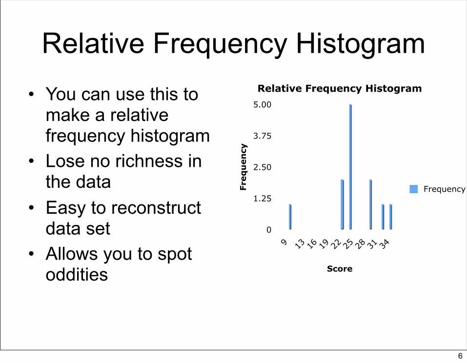
Relative Frequency Histogram• You can use this to

make a relative frequency histogram

• Lose no richness in the data

• Easy to reconstruct data set

• Allows you to spot oddities

0

1.25

2.50

3.75

5.00

9 13 16 19 22 25 28 31 34

Relative Frequency Histogram

Fre

qu

en

cy

Score

Frequency

6

Categorical Data

• With categorical data you do not get a histogram, you get a bar graph

• You could do a pie chart too, though I hate them (but I love pie)

• Pretty much the same thing, but the x axis really does not have a scale so to speak

• So say we have a STAT 2126 class with 38 Psych majors, 15 Soc, 18 CESD majors and five Bio majors

7

Like this

0

10

20

30

40

Psych Soc CESD Biology

STAT 2126

Co

un

t

Major

Biology

CESD

Soc

Psych

STAT 2126

8

Quantitative Variables

• So with these of course we use a histogram

• We can see central tendency• Spread• shape

9

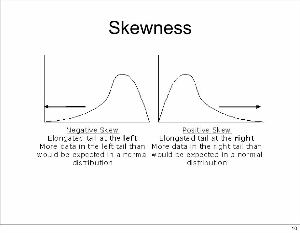
Skewness

10

Kurtosis

• Leptokurtic means peaked• Platykurtic means flat

11

More on shape

• A distribution can be symmetrical or asymmetrical

• It may also be unimodal or bimodal• It could be uniform

12

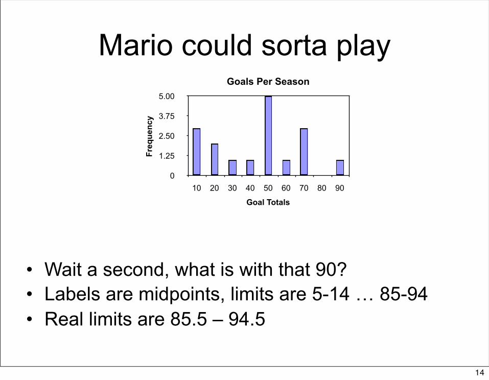
An example• Number of goals

scored per year by Mario Lemieux

• 43 48 54 70 85 45 19 44 69 17 69 50 35 6 28 1 7

• A histogram is a good start, but you probably need to group the values

13

Mario could sorta play

• Wait a second, what is with that 90?• Labels are midpoints, limits are 5-14 … 85-94• Real limits are 85.5 – 94.5

0

1.25

2.50

3.75

5.00

10 20 30 40 50 60 70 80 90

Goals Per Season

Freq

uenc

y

Goal Totals

14

Careful

• You have to make sure the scale makes sense

• Especially the Y axis• One of the problems with a histogram with

grouped data like this is that you lose some of the richness of the data, which is OK with a big data set, perhaps not here though

15

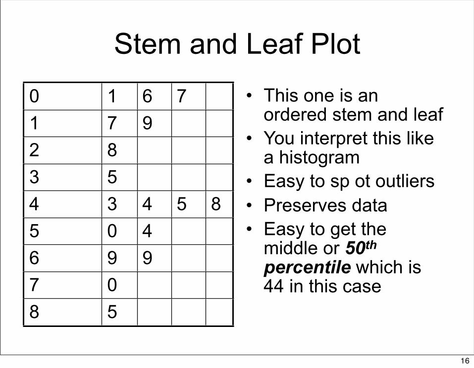
Stem and Leaf Plot

0 1 6 71 7 92 83 54 3 4 5 85 0 46 9 97 08 5

• This one is an ordered stem and leaf

• You interpret this like a histogram

• Easy to sp ot outliers• Preserves data• Easy to get the

middle or 50th percentile which is 44 in this case

16

The Five Number Summary

• You can get other stuff from a stem and leaf as well

• Median• First quartile (17.5 in our case)• Third quartile (61.5 here)• Quartiles are the 25th and 75th percentiles• So halfway between the minimum and the

median, and the median and the maximum

17

You said there were five numbers..

• Yeah so also there is the minimum 1• And the maximum, 85

– These two by the way, give you the range• Now you take those five numbers and

make what is called a box and whisker plot, or a boxplot

• Gives you an idea of the shape of the data

18

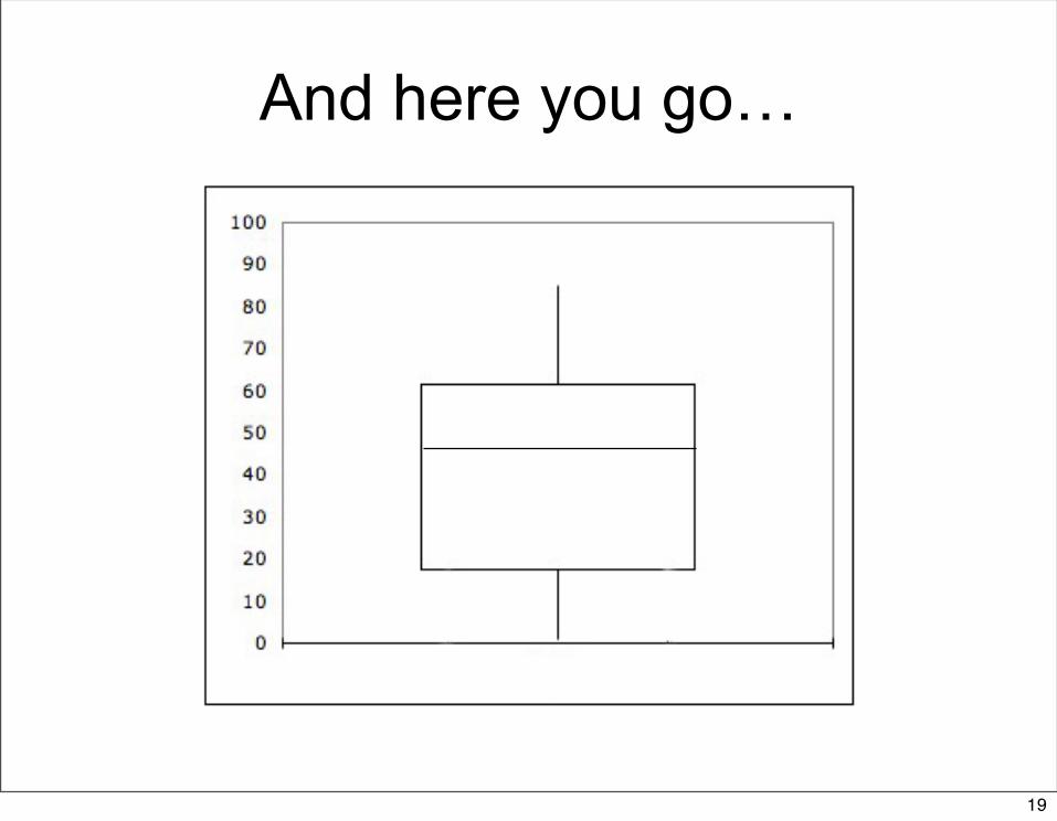
And here you go…

19

and it continues

• We talked about the central tendency of a distribution

• This is one of the three properties necessary to describe a distribution

• We can also talk about the shape– You know that kurtosis stuff and all of that

20

An Example

• Consider…• 1 5 9 20 30• 11 12 13 14 15• Both have the same mean (13)

– They both sum to 65, then divide 65 by 5, you get 13

21

The same, but different…

• 1 5 9 20 30• 11 12 13 14 15• So, they both have the same mean, and

both are symmetrical• How are they different?• Well the one on the top is much more

spread out

22

Spread

• Well how could we measure spreadoutedness?

• Well the range is a start• 1 - 30 vs 11 - 15• Seems pretty crude• We could look at the IQD• Still pretty crude

23

We need something better

• Something that is kind of like a mean really

• Like the average amount that the data are spread out

• Well why not do that?

24

Well here’s why not

€

(x − x)n∑ =

(1−13) + (5 −13) + (9 −13) + (20 −13) + (30 −13)5

=−12 + (−8) + (−4) + 7 +17

5

=05

25

Hmm

• They will ALWAYS sum to zero• Makes sense when you think about it• If the mean is the balancing point, there

should be as much mass on one side as the other

• So how do we get rid of negatives?• Absolute value!

26

The Mean Absolute Deviation

€

(x − x)n∑ =

(1−13) + (5 −13) + (9 −13) + (20 −13) + (30 −13)5

=12 + 8 + 4 + 7 +17

5

=485

= 9.6

27

Cool!

• Well sometimes things you think are cool, well they aren’t

• Mullets for example…• Anyway, for our purposes the MAD is

just not that useful• It is, in the type of stats we will do, a

dead end• Too bad, as it has intuitive appeal

28

There has to be another way

• Well of course there is or we would end now…

• OK, how else can we get rid of those nasty negatives?

• Square the deviations• (you know, -92 = 81 for example)

29

We are getting closer…

€

x − x( )2

n∑ =1−13( )2 + 5 −13( )2 + 9 −13( )2 + 20 −13( )2 + 30 −13( )2

5

=(−12)2 + (−8)2 + (−4)2 + 72 +172

5

=144 + 64 +16 + 49 + 289

5=112.4

30

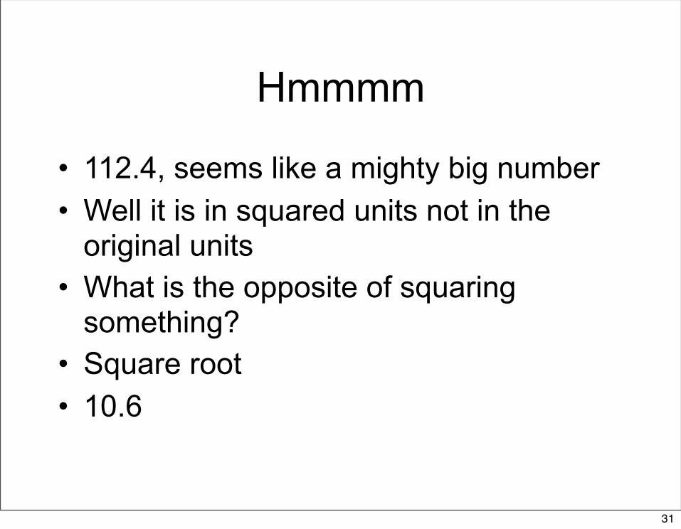
Hmmmm

• 112.4, seems like a mighty big number• Well it is in squared units not in the

original units• What is the opposite of squaring

something?• Square root• 10.6

31

There is a little problem here

• The formula I have shown you so far, has n on the bottom

• Yeah I know that just makes sense.• In fact, it is supposed to be n-1• We want something that will be an

unbiased estimator of the same quantity in the population

32

Variance and standard deviation

• The population parameters, variance and the standard deviation have N on the bottom

• The sample statistics used to estimate them have n-1

• If they had n, they would underestimate the population parameters

33

Sample statistics

€

s2 =x − x( )

2

n −1∑

€

s =x − x( )

2

n −1∑

34

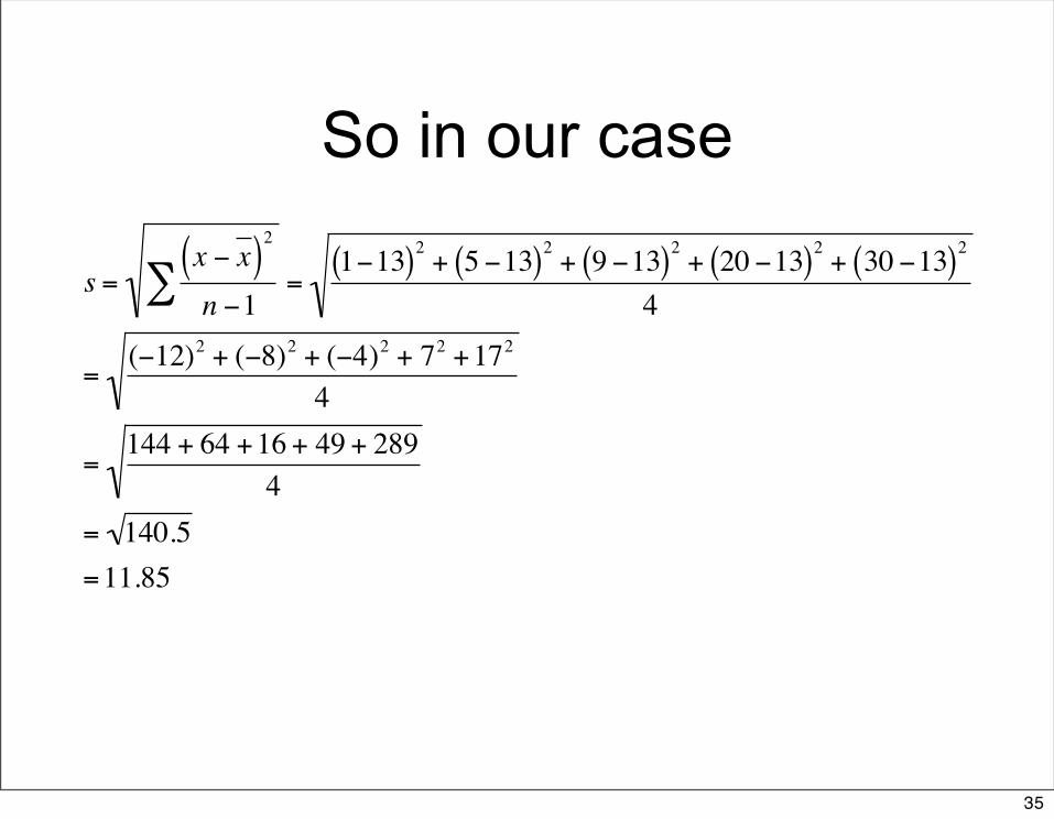
So in our case

€

s =x − x( )

2

n −1∑ =1−13( )2 + 5 −13( )2 + 9 −13( )2 + 20 −13( )2 + 30 −13( )2

4

=(−12)2 + (−8)2 + (−4)2 + 72 +172

4

=144 + 64 +16 + 49 + 289

4= 140.5=11.85

35

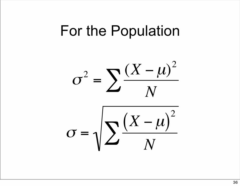
For the Population

€

σ =X −µ( )2

N∑€

σ 2 =(X −µ)2

N∑

36

How are the variance and sd affected by extreme scores?

• 1 5 9 20 30• s = 11.85• OK let’s throw in a new number, say 729• 1 5 9 20 30 729• Our new mean is 132.33• Our new variance is 85555.067• Our new standard deviation is 292.50• Well the mean is affected by extreme scores,

so of course so is the sd

37

How can we use this to our advantage?

• coefficient of variation• Katz et al (1990)• study mean 69.6 sd 10.6• no study mean 46.6 sd 6.8 • one could conclude there is more variation

with studying• however the cvs are .152 and .146

respectively• sd / mean

38

A couple of key points

• Remember, we want to learn about populations not samples

• we estimate population parameters with sample statistics

• we want unbiased estimators of parameters

39

39

€

E(x + k) = x + kvar(x + k) = sx

2

E(xk) = x kvar(xk) = sx

2k 2

Transformations

40

40