1

Exploiting the Full Potential of Microarray Data

X Liu*, V Vinciotti, K Fraser, S Swift and A Tucker*Leiden Institute of Advanced Computer Science, Leiden University; On leave fromSchool of Computing, Information Systems and MathematicsBrunel Universitywww.ida-research.net; hui@ida-research.net

Xiaohui Liu

Cell Nucleus: Where the genes are.

www.grad.ttuhsc.edu/courses/histo Texas Tech University Health Sciences Center

Genes are DNA sequences

DEFINITION Human breast cancer susceptibility (BRCA2) mRNA, complete cds.ORGANISM Homo sapiens

Eukaryotae; mitochondrial eukaryotes; Metazoa; Chordata;Vertebrata; Eutheria; Primates; Catarrhini; Hominidae; Homo.

FEATURES Location/Qualifierssource /map="13q12-q13"

/chromosome="13"CDS 229..10485

/gene="BRCA2"/codon_start=1/product="BRCA2"

/gene="BRCA2”ORIGIN

1 ggtggcgcga gcttctgaaa ctaggcggca gaggcggagc cgctgtggca ctgctgcgcc61 tctgctgcgc ctcgggtgtc ttttgcggcg gtgggtcgcc gccgggagaa gcgtgagggg

121 ctcgggtgtc ggtggcgcga gaggcggagc cgctgtggca atccaaactc gccgggagaa[180 lines deleted] 10921 ttacaatcaa caaaatggtc atccaaactc aaacttgaga aaatatcttg ctttcaaatt10981 gacacta

www.ncbi.nlm.nih.gov/Entrez

2

Protein

mRNA

DNA

transcription

translation

CCTGAGCCAACTATTGATGAA

PEPTIDE

CCUGAGCCAACUAUUGAUGAA

MicroarrayIndividual genes can be compared using a ‘Competitive Hybridisation’Microarrays allow this experiment to be carried out on a mass scale at a microscopic levelTypically 6-30 thousand genes can be analysed on one chip simultaneouslyCy5

Cy3

Cy5

Cy3

+ +

+ +

Extract RNA

Treated Cell

Normal Cell

Human Genome

Dye

Print Array

cDNA microarrays: the processBuilding the chip:

MASSIVE PCR PCR PURIFICATION and PREPARATION

PREPARING SLIDES PRINTING

RNA preparation:

CELL CULTURE AND HARVEST

RNA ISOLATION

cDNA PRODUCTION

Hybing the chip: POST PROCESSING

ARRAY HYBRIDIZATION

PROBE LABELING

SCANNING THE CHIP

Adapted from Schena & Davis

3

cDNA microarrays: Building the chip

Arrayed Library(96 or 384-well plates)

PCR amplification Consolidate into well plates

Spot as microarrayon glass slides

(Ngai Lab, UC Berkeley)

96 well plate Contains cDNA probes

Glass SlideArray of bound cDNA probes

4x4 blocks = 16 print-tip groups

Print-tip group 7

Print-tip group 1

Pins collect cDNA from wells

cDNA microarrays: RNA preparation

mRNA is reverse-transcribed into cDNA and labelled.

cDNA microarrays: Hybing the chipHybridizing of labelled cDNA target samples to cDNA probes on the slide

cover

slip

Hybridize for

5-12 hours

4

cDNA microarrays: brief summary

cDNA “A”Cy5 labeled

cDNA “B”Cy3 labeled

Hybridization Scanning

Laser 1 Laser 2

+

Image Capture

Biological Question

Sample PreparationMicroarray

Life Cycle

Data Analysis & Modelling

MicroarrayReaction

MicroarrayDetection

Taken from Schena & Davis

Biological questionCo-expressed genes

Sample class prediction etc.

Testing

Biological verification and interpretation

Microarray experiment

Estimation

Experimental design

Image analysis

Low-level analysis

Clustering Discrimination

16-bit TIFF files

Microarray gene expression Data

Gene expression data on p genes for n samples

Genes

mRNA samples

Gene expression level of gene i in mRNA sample j

=Log( Red intensity / Green intensity), or

sample1 sample2 sample3 sample4 sample5 …1 0.46 0.30 0.80 1.51 0.90 ...2 -0.10 0.49 0.24 0.06 0.46 ...3 0.15 0.74 0.04 0.10 0.20 ...4 -0.45 -1.03 -0.79 -0.56 -0.32 ...5 -0.06 1.06 1.35 1.09 -1.09 ...

Log(Signal)

5

Veronica Vinciotti

From experimental design to gene networks

Sample A Sample B

RNA

cDNA

Cy3-dCTP Cy5-dCTP

DNAmicroarray

A=BA < B

A > B

DATAEXPERIMENTALDESIGN

IMAGEANALYSIS

CLUSTERING/CLASSIFICATION

BIOLOGICALNETWORKS

TWO-CHANNEL DNA MICROARRAY EXPERIMENT

Experimental Design Experimental Design Issues

Technical variationReplicated genes on the slide

Biological variationSamples from different individuals

How to allocate samples to arraysWhich two conditions should be compared on one array?

6

Choice of DesignQuestion: Given number of conditions (e.g. time points) we wish to compare and a number of arrays we can afford to make, what is the most efficient design?

Which Design is Best?Loop-type of designs have been shown to be more efficient than reference designs

Both theoretically and experimentallyLoop designs allocate the resources more efficiently to compare the conditions of interest

In a reference design, 50% of the resources are used on a reference sample, of little interest to biologists

However…The data that come out of loop-type of designs are less intuitive

One can use a simple linear model to obtain estimates of the contrasts

How to extend loop designs to large studiesComparing all possible pairs of conditions becomes unrealistic for large studies

How to measure the efficiency of a designThe design should provide precise estimates of the parameters of interestThe design should be robust to the situation when arrays get missing/damaged or the experiment has to be extended in future

Design for Large Studies(Vinciotti et al, 2004, Bioinformatics)

7

Karl Fraser

Current Image Processing Techniques

Current techniques rely upon operator assistance and prior knowledgeAt present, no one method has been successful in blindly processing a slide with excess noiseRather than focus on one technique, we instead propose an adaptable framework which can be developed to combine multiple techniques

Current ProcessingGenePix® Method

Current Processing…contGenePix® Method

8

Problems Copasetic Analysis

Image Layout

Acquire high level image information

(gene blocks)

Image Layout

Acquire high level image information

(gene blocks)

Image Structure

Acquire low level image information (individual genes)

Image Structure

Acquire low level image information (individual genes)

Copasetic Clustering

Applies a clustering algorithm to the entire

image surface

Copasetic Clustering

Applies a clustering algorithm to the entire

image surface

Structure Extrapolation Feature Identification

Final Analysis

Summarise data (calculate gene spot metrics)

Final Analysis

Summarise data (calculate gene spot metrics)

Final Analysis

Summarise data (calculate gene spot metrics)

Data Services Data Analysis

Post Processing

Clean up image (compensate for

background noise)

Post Processing

Clean up image (compensate for

background noise)

Post Processing

Clean up image (compensate for

background noise)

Imag

e T

ran

sfo

rmat

ion

En

gin

e

Tra

nsfo

rm im

ages

into

diff

eren

t vie

ws

as

requ

ired.

Thi

s se

rvic

e is

ava

ilabl

e to

all

subs

eque

nt s

tage

s of

the

fram

ewor

k

Imag

e T

ran

sfo

rmat

ion

En

gin

e

Tra

nsfo

rm im

ages

into

diff

eren

t vie

ws

as

requ

ired.

Thi

s se

rvic

e is

ava

ilabl

e to

all

subs

eque

nt s

tage

s of

the

fram

ewor

k HISTORICAL RESULTS

FINAL RESULTS

Data Stream

Service Request Helper Task

Core TaskData StreamData Stream

Service RequestService Request Helper Task

Core TaskOutput

Log2 ratios and related statistics

Output

Log2 ratios and related statistics

Input

Raw 16bit cDNA microarray

images

Spatial Binding

Identify and group regions of interest (a genes pixels)

Spatial Binding

Identify and group regions of interest (a genes pixels)

Vader Search

Enhance ‘Spatial Binding’ using

historical results

Vader Search

Enhance ‘Spatial Binding’ using

historical results

ITE: Data Filtering

Analysing the raw data may not be beneficialFiltering can clean, emphasis genesFor example, input-output response curves

Filtered DataRaw Data

ITE: Data Transformations

Sometimes a different perspective can help…

9

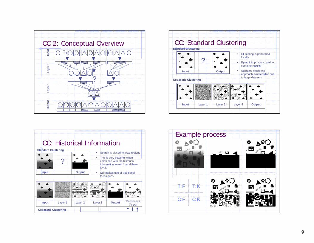
CC 2: Conceptual OverviewIn

put

Out

put

Laye

r 0La

yer 1

?

CC: Standard ClusteringStandard Clustering

Copasetic Clustering

• Clustering is performed locally

• Pyramidic process used to combine results

• Standard clustering approach is unfeasible due to large datasets

Input Output

?

Input Layer 1 Layer 2 Layer 3 Output

CC: Historical Information

Input Output

?• Search is biased to local regions

• This is very powerful when combined with the historical information saved from different levels

• Still makes use of traditional techniques

Input Layer 1 Layer 2 Layer 3 Output Consensus Output

Copasetic Clustering

Standard Clustering

T:KT:KT:FT:F

C:KC:KC:FC:F

Example process

10

CC: Microarray Results

• A microarray slide that contains ~10 million observations (1.2M FG)• Black squares show regions where extreme values have distorted local area

Post-Processing & Final Analysis

Overall Results

Provided a 1 – 3dB (PSNR) improvement over GenePix® as used by an expert operator

HGMP 1 HGMP 2

Stephen Swift

11

Clustering and Grouping (1)

ClusteringArranging Objects (as Points) into Sets According to “Distance” on a Hyper-Graph

GroupingArranging Objects into Sets According to Some Inter-Object Relationship

Each Set is Usually Mutually Exclusive

Will Not Consider “Fuzzy” Clustering

Clustering and Grouping (2)

Problem

Clustering Grouping

DistanceMatrix

RelationshipMatrix

ClusterWorth

ClusteringMethod

Application 1 – MTS Decomposition

-3

-2

-1

0

1

2

3

1 7 13 19 25 31 37 43 49 55 61 67 73 79 85 91 97

-2.5-2

-1.5-1

-0.50

0.51

1.52

1 8 15 22 29 36 43 50 57 64 71 78 85 92 99

-3

-2

-1

0

1

2

3

1 7 13 19 25 31 37 43 49 55 61 67 73 79 85 91 97

Application 2 – Email Logfiles

SITE A-02SITE A-01 SITE A-03 SITE A-04 SITE A-05

SITE A

SITE B-01 SITE B-02

SITE B

SITE C-02SITE C-01 SITE C-03 SITE C-04 SITE C-05

SITE C

SITE D-01 SITE D-02 SITE D-03

SITE D SITE X-YZ

SITE X

KEY

Server Name

Server

Network Connection

Physical Site

Site Name

12

Application 3 – Microarrays Vectors and Distances (1)

Many Methods are Designed to Work on Distance Metrics, e.g. K-Means

They Assume that the “Triangle Inequality” Holds

This is NOT the Case for Many Applications, e.g. MTS Decomposition Using Cross-Correlation

More General “Grouping” Methods Must be Chosen

Vectors and Distances (2)Distance Matrices

Euclidean

Correlation

Minkowski

Manhattan

Mahalanobis

Relationship MatricesHow Long is a Piece of String?

Often Application Dependant

Cluster Worth (1)

The Choice of Correct Metric for Judging the Worth of a Clustering Arrangement is Vital for Success

There are as Many Metrics as Methods!

Each has Their Own Merits and Drawbacks

13

Cluster Worth (2)

Sum of Squares by Cluster

Homogeneity (H)

Separation (S)

H/S

Maximum Likelihood

Minimum Description Length

Etc…

The Number of ClustersMany Applications Specify the Number of Clusters a Solution Requires, e.g. the Email Server Application

Many Do Not, e.g. Microarray Data

Determining the Number of Clusters is Very Difficult

A Choice of Method that Locates the Number of Clusters and Their Contents is Often Desirable

MethodsStatistical

K-Means

Hierarchical

PAM

Optimisation / Search /AIEvolutionary Computing

SOM

Hill Climbing and Simulated Annealing

KDD and Others, e.g. CLARIS, EM

Comparing Clusters and Methods

H40 K40 SOM40 HC40 SA40

H40 - 0.609 0.041 0.640 0.647

K40 - - 0.053 0.536 0.540

SOM40 - - - 0.082 0.074

HC40 - - - - 0.879

SA40 - - - - -

Metrics Can Be Used To Compare Method Result Similarity

14

Consensus Clustering

Clustering Results Can Vary Depending on the Method UsedCombine the Results of Multiple Methods into One Set of Consensus ResultsAn Algorithm is Needed For Generating Consensus Clusters Given the Agreement MatrixWe Use an Approximate Stochastic Algorithm Called Simulated Annealing

Consensus Clustering

Agreement MatrixConsensus Clusters

Input Cluster Results

-10 0 10 20

-10

-50

5

cmdscale(disthhv8)[,1]

cmds

cale

(dis

thhv

8)[,2

]

-10 0 10 20

-10

-50

5

cmdscale(disthhv8)[,1]

cmds

cale

(dis

thhv

8)[,2

]

-10 0 10 20

-10

-50

5

cmdscale(disthhv8)[,1]

cmds

cale

(dis

thhv

8)[,2

]

-10 0 10 20

-10

-50

5

cmdscale(disthhv8)[,1]

cmds

cale

(dis

thhv

8)[,2

]

The Agreement Matrix Scalability Issues

0.75

0.85

0.95

0 500 1000 1500 2000

N

WK

K-MeansHCM1SAM1HCM2SAM2

15

Summary (1)

Clustering and Grouping Problems are Hard!

Especially Microarray Data

Difficult Choice of Metric, Cluster Worth and Method Against Problem

There is No Free Lunch!

Allan Tucker

MicroArray Data

High dimensionalSmall number of samplesModel the data

ClassificationFeature selectionKnowledge discovery

Model complexity issues

Effect of Model Complexity

sample size

aver

age

CV

err

or

20 40 60 80 100

0.0

0.2

0.4

0.6

0.8

1.0 5 links

50 links500 linksNaive

(a)

16

Identifying Predictive Genes

Naïve Bayes ClassifierWell establishedMinimises parameters

Feature selectionLocal stepwise methodsGlobal search (SA)

Resampling methodsCross validation

Identifying Predictive Genes

Identify genes robustlyData perturbed during CVRepeats of stochastic SA search

Assign confidence based upon the frequencies of genes being selectedLimit maximum number of links -MDL

Confidence Scores

Relatively small number of genes Identified with high confidenceConsistency between runs

genes

prop

ortio

n

0 200 400 600 800 1000 1200 1400

0.0

0.2

0.4

0.6

0.8

1.0

genes

prop

ortio

n

0 100 200 300 400 500 600

0.0

0.2

0.4

0.6

0.8

1.0

Identified GenesB-CELL PROSTATE

GeneBank Proportion GeneBank ProportionAK023995 0.862 AA055368* 0.5U15173* 0.796 N64741 0.34L21936 0.488 AA487560* 0.33D83785 0.454 W47179 0.27

BC014433 0.442 AA486727 0.26U59309 0.277 AA455925 0.25-47202 0.25 H29252 0.25

Z14982* 0.169 AA010110 0.24BC016182* 0.162 AA180237 0.23

U82130 0.146 AA443302 0.2Z80783 0.131

BC009914 0.127U77949 0.112

17

Expert Knowledge

Lots of other information availablePathway InformationGene OntologySequence InformationFunctional information

Use this data as prior knowledgeUpdate with data

Bayesian Classifiers

TAN - No longer assume independence between features

BNC – Include class node as a normal variable

Dynamic Bayesian Networks

g0

g1

g2

g3

g4

t-5 t-4 t-3 t-2 t-1 t

Genes

Time Lag

Summary (2)

When micro-array data only has small samples:

Simple models with small parameters bestGlobal search for parameters better

Bayesian networks can incorporate different types of dataUpdate expert knowledge with data

18

Conclusion

Biological data are very noisy Modelling biological systems, at systems level?More integrated computational methods for organising and analysing data

Acknowledgements

LIACS, LUMC, IBLMARIE, BIOMAP, BBSRC, EPSRC, Wellcome

TrustLarry Hunter, Terry SpeedData kindly provided by

Paul Kellam from the Dept. of Immunology and Molecular Pathology, University College London.Dr Li from the Dept. of Biological Sciences, BrunelUniversity, Uxbridge.