explicit stress integration of complex soil...

INTERNATIONAL JOURNAL FOR NUMERICAL AND ANALYTICAL METHODS IN GEOMECHANICSInt. J. Numer. Anal. Meth. Geomech., 2005; 29:1209–1229Published online 12 July 2005 in Wiley InterScience (www.interscience.wiley.com). DOI: 10.1002/nag.456

Explicit stress integration of complex soil models

Jidong Zhao1,n,y, Daichao Sheng1, M. Rouainia2 and Scott W. Sloan1

1School of Engineering, University of Newcastle, NSW 2308, Australia2School of Civil Engineering and Geosciences, University of Newcastle, Newcastle upon Tyne NE1 7 RU, U.K.

SUMMARY

In this paper, two complex critical-state models are implemented in a displacement finite element code. Thetwo models are used for structured clays and sands, and are characterized by multiple yield surfaces, plasticyielding within the yield surface, and complex kinematic and isotropic hardening laws. The consistenttangent operators}which lead to a quadratic convergence when used in a fully implicit algorithm}aredifficult to derive or may even not exist. The stress integration scheme used in this paper is based on theexplicit Euler method with automatic substepping and error control. This scheme employs the classicalelastoplastic stiffness matrix and requires only the first derivatives of the yield function and plasticpotential. This explicit scheme is used to integrate the two complex critical-state models}the sub/super-loading surfaces model (SSLSM) and the kinematic hardening structure model (KHSM). Variousboundary-value problems are then analysed. The results for the two models are compared with each other,as well with those from standard Cam-clay models. Accuracy and efficiency of the scheme used for thecomplex models are also investigated. Copyright # 2005 John Wiley & Sons, Ltd.

KEY WORDS: explicit stress integration; automatic substepping; critical state models; bounding surface;structured soil

1. INTRODUCTION

Critical-state soil models were first developed by Roscoe and his colleagues at Cambridge 30years ago [1–4]. Since then, such models have been widely used in various geotechnicalapplications. Despite their popularity, the classic Cam-clay models are inadequate foraddressing soil characteristics such as structures, anisotropy, small-strain behaviour, stiffnessdegradation during cyclic loading, and rate-dependent behaviour. Consequently, a variety ofcomplex elastoplastic models have been proposed and they contain various modifications to thestandard Cam-clay models to cover different soil types and loading behaviours [5–10]. Inparticular, the kinematic hardening structure model (KHSM) developed by Rouainia and MuirWood [9] and the sub/super-loading surface model (SSLSM) proposed by Asaoka [10] are bothcapable of addressing natural soils with initial structures, and can simulate complicated soilresponse during cyclic loading. However, these models are mostly used to model the behaviour

Received 2 September 2004Revised 22 May 2005

Accepted 24 May 2005Copyright # 2005 John Wiley & Sons, Ltd.

yE-mail: [email protected]

nCorrespondence to: J. Zhao, School of Engineering, University of Newcastle, NSW 2308, Australia.

of one single soil element and their applications to boundary-value problems are rather limited.The aim of the present study is to develop algorithmic and computational aspects of finiteelement implementation of the two models using an explicit stress-integration scheme.

Existing approaches for integrating stress–strain laws at Gauss points can be classified as‘explicit’ schemes or ‘implicit’ schemes. Implicit algorithms based on the concepts of operatorsplit and closest point projection or the so-called return mapping have been applied to a varietyof computational geomechanics applications [11–22], while explicit schemes with substeppingand error control have also been suggested in References [23–28] and applied to variousgeotechnical problems [7,29,30]. The advantages and disadvantages of the two classes ofschemes are well-known and extensive comparisons between them have been made in literature(see, e.g. References [27,30–33]).

While both implicit and explicit schemes have been developed for the classic critical-statemodels [7,12,14–17,20], application of these schemes to more complex geomechanical models islimited. It is generally fair to state that highly non-linear complex constitutive models favours anexplicit solution, because (i) the numerical solution to the local non-linear equations in animplicit scheme may not converge, (ii) the consistent tangent operator may be very difficult toderive so that the main advantage of the implicit schemes, i.e. the quadratic convergence ofNewton iteration, is not guaranteed. In addition, certain geomechanical models, as the twomodel used in this paper, become so complex that it is very difficult to derive the second-orderderivative of the plastic potential. Some exceptions of using implicit schemes for complexmodels include Bojar et al. [20] and Tamagnini et al. [21]. The former has used implicit schemeto solve an anisotropic bounding surface model. A loading surface that is homologous to thebounding surface in the strain space has to be introduced to handle the additional consistencycondition on the bounding surface. Tamagnini et al. [21] used an implicit generalized backwardEuler (GBE) method to treat an elastoplastic constitutive model for bonded geomaterials. Someassumptions such as material isotropy and hyperelastic behaviour had to be made to partiallyalleviate the drawbacks of implicit algorithms such as the requirement of computing the second-order gradients of the plastic potential.

On the other hand, it is less cumbersome to use explicit integration schemes to solve complexconstitutive models. In particular, the accuracy of these schemes, which is perceived to be theirmain drawback compared to the implicit schemes, can be overcome by using automaticsubstepping and error control. In this paper, the explicit scheme presented in References [26,27]is extended to solve two complex models. The two models KHSM and SSLSM both containmultiple yield surfaces and combined kinematic and isotropic hardening, invoked by theintroduction of an initial structure and the bounding surfaces. The explicit scheme isreformulated to accommodate additional internal variables and hardening laws. Theconsistency conditions on the bounding surfaces are translated to the current loading surfaces.No addition measure is required to treat the consistency associated with the bounding surface.An automatic load stepping scheme is used to solve the global system of Equations [28,29],which ensures that the small-strain non-linearity in the KHSM and SSLSM is captured withaccuracy and efficiency.

This paper is organized as follows. First, the KHSM and the SSLSM are briefly described andcompared. Secondly, a general procedure for integrating stress–strain laws with both kinematicand isotropic hardening and more than one hardening parameters is presented. Thirdly, the twoconstitutive models are used to analyse triaxial compression tests under drained and footingconditions. The results of the two models are compared, as well as those from standard

Copyright # 2005 John Wiley & Sons, Ltd. Int. J. Numer. Anal. Meth. Geomech. 2005; 29:1209–1229

J. ZHAO ET AL.1210

Cam-clay models. The performance of the explicit substepping integration scheme on KHSMand SSLSM is evaluated. Finally, the conclusions of the study are summarized.

2. TWO COMPLEX SOIL MODELS

In this section, the KHSM (Rouainia and Muir Wood [9]) and the SSLSM (Asaoka [10]) arebriefly described. Slight modifications have been made to the formulation of each of the modelsto facilitate comparison. Both the KHSM and SSLSM were developed to account for initialstructures, small strain stiffness, stiffness degradation with strain history, and hystereticresponse in cyclic loading. In the KHSM, this was done by adding a structural surface into thekinematic hardening model developed by Al-Tabbaa and Muir Wood [34]; while in the SSLSM,an extra superloading surface was introduced into the subloading surface model proposed byHashiguchi [35]. Concepts of bounding-surface plasticity [36] are used in both models. As aresult, there are three surfaces of elliptical shape as in the MCC model in both models}thereference surface, the bubble surface, and the structural surface for the KHSM (see Figure 1(a)in the plane of p0 � q) and the normal yield surface, the subloading surface, and thesuperloading surface for the SSLSM (see Figure 1(b)). The small elastic region is confined by asmall kinematic hardening bubble in the KHSM and the subloading surface in the SSLSM,respectively. The current stress state is always located within or on the bubble/subloadingsurface. Any stress path moving beyond the initial boundary of the bubble/subloading surfacecauses plastic deformation and evolution of all yield surfaces. The KHSM was initiallypresented in a form that can account for the initial anisotropy in soils by presenting a structuresurface not passing through the origin. For simplicity, this feature is neglected here}with boththe structure surface and the reference surface being assumed to pass through the origin.Consequently, it has a formulation similar to the model proposed by Muir Wood [6]. In theSSLSM, the three yield surfaces are all supposed to pass through the origin.

In both models, associated flow is assumed. The yield functions and corresponding plasticpotentials for the yield surfaces in the two models are presented in Table I. In Table I, p0 and s

are the mean pressure and the deviatoric stress, respectively, given by p0 ¼ tr½r�=3; s ¼ r� pI;where I is the second-order identity tensor and tr½�� is the trace operator of ½��: For SSLSM,

q

p′ cp′ cp′ ~ cp′

( )qp , ( )qp ,

Superloading Surface

Normal yield Surface

Subloading Surface

O

p′Mq =

( )qp ~,~

(b)

q

p′ cp′ ˆp′

cb p′r

Reference Surface

Critical state line

cs pr ′

Bubble Surface

c

nn

Structure Surface

O

(a)

σσ

α

′′′

�

Figure 1. Illustration of yield surfaces for KHSM and SSLSM in the p0–q plane:(a) KHSM [9]; (b) SSLSM [10].


EXPLICIT STRESS INTEGRATION OF COMPLEX SOIL MODELS 1211

ðp0; sÞ; ð%p0;%sÞ and ð*p0; *sÞ are the mean pressure and deviator stress at the subloading surface,superloading surface and normal-loading surface, respectively. Relations among them will beaddressed afterwards. It should be noted that the slope of the critical state line (CSL)(designated by M in the table) is expressed as a function of the Lode angle y; and determines theshape of the failure surface in the deviatoric plane. The following expression for M is used inthis paper:

MðyÞ ¼Mmax2a4

1þ a4 � ð1� a4Þsin 3y

� �1=4ð1Þ

By setting the parameter a with a ¼ ð3� sin fÞ=ð3þ sin fÞ; this yield surface coincides with theMohr–Coulomb hexagon at all vertices in the deviatoric plane (where f is the friction angle ofthe soil at critical state), while setting a ¼ 1; recovering the Drucker–Prager compression circle.It should be noted that this surface is differentiable for all stress states and is convex (provideda50:6). The variation of yield surface cone with respect to a in the deviatoric stress plane isdepicted in Figure 2.

Other parameters in Table I should be noted in conjunction with Figure 1. For the KHSM,ðp0c; 0Þ; ðp

0#a; 0Þ; and ðp

0%a; s%aÞ (instead of ðp0%a; q%aÞÞ are the centres of the reference surface in a general

3D stress space, the structure surface, and the bubble surface in a general 3D stress space,respectively. Rs ¼ p0#a=p

0c is a parameter indicating the initial structure, whereas Rb is the size

ratio of the bubble surface over the reference surface (and is assumed to be constant duringloading). The KHSM uses the slopes of the normal compression line and swelling line, ln andkn; in the plane of ln v� ln p0; which is slightly different from standard critical-state models. Forthe SSLSM, ðp0c; 0Þ; ð*p

0c; 0Þ; and ð%p

0c; 0Þ are the respective centres of the three surfaces. Moreover,

ðp0; qÞ; ð*p0; *qÞ; and ð%p0; %qÞ are the corresponding stresses on the subloading, normal Cam-clay, andsuperloading yield surfaces in the p0–q plane, respectively. The three stress states are related to

Table I. Yield functions and corresponding plastic potentials for KHSM and SSLSM.

Model Yield surface Yield function and plastic potential

KHSM [9] Reference surface fr ¼ gr ¼s : s

ðMðyÞp0cÞ2þ

p0

p0c� 1

� �2

�1

Bubble surface fb ¼ gb ¼ðs� s%aÞ : ðs� s%aÞ

ðMðyÞp0cÞ2

þp0 � p0%a

p0c

� �2

�R2b

Structure surface fs ¼ gs ¼s : s

ðMðyÞp0cÞ2þ

p0

p0%c� Rs

� �2

�R2s

SSLSM [10] Normal yield surface fnor ¼ gnor ¼*s : *s

ðMðyÞ*p0cÞ2þ

*p0

*p0c� 1

� �2

�1

Subloading surface fsub ¼ gsub ¼s : s

ðMðyÞp0cÞ2þ

p0

p0c� 1

� �2

�1

Superloading surface fsup ¼ gsup ¼%s : %s

ðMðyÞ%p0cÞ2þ

%p0

%p0c� 1

� �2

�1


J. ZHAO ET AL.1212

one another by the following radial mapping rule:

R ¼p0

%p0¼

q

%q; Rn ¼

*p0

%p0¼

*q

%qð2Þ

where R and Rn are similarity ratios for superloading/subloading surfaces and superloading/normal surfaces, respectively. They act as constitutive hardening variables in the SSLSM. IfR ¼ Rn ¼ 1:0; the SSLSM will coincide with the modified Cam-clay model (MCCM). If in amore general 3D stress place, ðp0; qÞ; ð*p0; *qÞ; and ð%p0; %qÞ may be replaced by ðp0; sÞ; ð%p0;%sÞ and ð*p0; *sÞ;respectively, where s; %s and *s have a same principal direction and yield a similar relations innorm form as (2) R ¼ jjsjj=jj%sjj; Rn ¼ jj*sjj=jj%sjj:

The elastic moduli present themselves in the KHSM and the SSLSM in the following form:

KHSM : K ¼dp0

deev¼

p0

kn

SSLSM : K ¼dp0

deev¼

vp0

k

; G ¼3ð1� 2mÞ2ð1þ mÞ

K ð3Þ

where K and G are the bulk modulus and the shear modulus, respectively. eev denotes the elasticvolumetric strain. m is Poisson’s ratio. v ¼ 1þ e is the specific volume, and e is the void ratio.

The evolution of the plastic strain in the KHSM and the SSLSM is the same as in thestandard Cam-clay model:

depij ¼ dg@g

@s0ijð4Þ

where depij denotes the plastic strain increment, dg denotes the plastic multiplier. The followinggeneralized form of hardening laws is supposed for both models:

dj ¼ dgB ð5Þ

where j denotes a vector of hardening variables and B is an intermediate vector used in thefinite element formulation. In the KHSM the size of the bubble with respect to the reference

2

Mohr-Coulomb

ο30

ο30

Eq. (1)

Drucker-Prager Compression

Cone (� =1 )

−

�

�′3�′

1�′

Figure 2. Variation of the yield surface with respect to a in the deviatoric stress plane.



surface can be assumed to be constant, so that rb ¼ const: In this case the KHSM has fourhardening parameters: p0c; rs; and the bubble centre ðp0%a; s%aÞ: In the SSLSM, there are threehardening parameters: p0c; R; and Rn: Thus the vectors j and B in the two models have thefollowing expressions:

KHSM : j ¼ fk1;k2;k3;k4gT ¼ fp0c;Rs; p0%a; s%ag

T; B ¼ fB1;B2;B3;B4gT

SSLSM : j ¼ fk1;k2;k3gT ¼ fp0c;R;R

ngT; B ¼ fB1;B2;B3gT

ð6Þ

Detailed expressions for the elements of B in the KHSM and the SSLSM may be referred to inAppendix A.

In the KHSM, the following geometric kinematic hardening mapping rule is used to ensurethe movement of the bubble in a direction parallel to the line joining the current stress and theconjugate point on the bounding surface:

%rc

Rs¼

%rRb

ð7Þ

where %rc ¼ rc � #a; %r ¼ r� %a; r and rc denotes the current stress on the bubble and itsconjugate stress point (image stress) on the structure surface, respectively. In addition, theplastic modulus H in the KHSM is assumed to depend on the Euclidean distance b between thecurrent stress and the conjugate stress (as illustrated in Figure 3).

It should be noted that both models can degenerate to the standard Cam-clay model byappropriate selection of model parameters. The MCC model will be recovered by the KHSMwith Rb ¼ Rs ¼ 1:0; and by the SSLSM with R ¼ Rn ¼ 1:0: In addition, both models use thesame the destructuration laws Rn ¼ 1=Rs; given k ¼Ma; ln ¼ l=v; kn ¼ k=v and under the sameplastic deformation index (for example, ed in this paper), where Rs and Rn are thedestructuration index in the KHSM and SSLSM, respectively. However, the two models alsoexhibit obvious differences, in such aspects as the anisotropic nature of the model itself, themapping rule, and the description of the reconsolidation process for soils. Details may bereferred to in [9,10].

q

p′ cp′

c

nn

O

b

α

ασ

σ

Figure 3. Illustration of the translation rule and normalized distance for KHSM.


J. ZHAO ET AL.1214

3. EXPLICIT STRESS INTEGRATION

3.1. General formulation for finite element implementation

During a typical elastoplastic finite element analysis, the following system of ordinarydifferential equations is to be solved:

’r ¼ Dep’e

’j ¼ ’gBð8Þ

where ’r and ’e are the rate of the stress and strain, respectively. ’j ¼ f’k1; ’k2; . . . ; ’kngT denotes the

rate of the hardening parameter vector, and BT ¼ f@k1=@g; @k2=@g; . . . ; @kn=@gg: The elasto-plastic stiffness matrix and plastic multiplier are defined through

Dep ¼ De �Deba

TDe

Aþ aTDeb; ’g ¼

aTDe’eAþ aTDeb

ð9Þ

where De is the elastic stiffness matrix. For the two models to be implemented, expressions inEquation (3) are used for K and G: The generalized hardening modulus A and the gradients ofyield surface and plastic potential are defined by

A ¼ �@f

@j

� �T’j’g; a ¼

@f

@r; b ¼

@g

@rð10Þ

The generalized hardening modulus A in the KHSM has the following form:

A ¼ �@fb@p0c

@p0

@epv

@fb@p0¼

@fb@p0%a

@p0%a@edþ@fb@q%a

@q%a@ed

� � ffiffiffiffiffiffiffiffiffiffiffiffiffiffiffiffiffiffiffiffiffiffiffiffiffiffiffiffiffiffiffiffiffiffiffiffiffiffiffiffiffiffiffiffiffiffiffiffiffiffiffiffiffiffiffið1� AdÞ

@fb@p0

� �2þAd

@fb@q

� �2sð11Þ

whereas in the SSLSM, it can be expressed as

A ¼ �@fsub@p0c

@p0c@*p0c

@*p0c@epv

@fsub@p0�@fsub@p0c

@p0c@R

@R

@edþ@p0c@Rn

@Rn

@ed

� � ffiffiffiffiffiffiffiffiffiffiffiffiffiffiffiffiffiffiffiffiffiffiffiffiffiffiffiffiffiffiffiffiffiffiffiffiffiffiffiffiffiffiffiffiffiffiffiffiffiffiffiffiffiffiffiffiffiffiffiffiffið1� AdÞ

@fsub@p0

� �2þAd

@fsub@q

� �2sð12Þ

The following pseudo-time, T ; is defined to facilitate the integration of (8)

T ¼ ðt� t0Þ=Dt ð13Þ

where t0 is the time at the start of the load increment, t0 þ Dt is the time at the end of loadincrement, and 04T41: Since dT=dt ¼ 1=Dt; (9) may then be rewritten as

drdT¼ DepDe ¼ Dr� DgDeb

djdT¼ ’gDtB ¼ DgB

ð14Þ



jidong

Cross-Out

jidong

Replacement Text

-

where Dg ¼ aTDreðAþ aTDebÞ: Equations (13) and (14) define a classical initial value problemto be integrated over the pseudo-time interval T ¼ 0 to 1.

3.2. Explicit stress integration

The explicit integration scheme with automatic substepping and error control [26,27] is usedhere to integrate the rate form of the stress–strain relations for the two models. A generalprocedure of this scheme include: (a) locating the yield surface intersection with the elastic trialstress path; (b) integrating the stress–strain relations using the modified Euler scheme withsubstepping and error control; and (c) correcting the yield surface drift if any. The proceduresfor implementing the KHSM and SSLSM closely follow that described in Reference [27] andonly the necessary modifications are given below.

3.2.1. Yield surface intersection. An elastic trial stress increment Dre is first computed upon theimposed strain increments De:

Dre ¼ DeDe ð15Þ

For both the KHSM and SSLSM, the elastic part of the constitutive relation is non-linear.However, the incremental relation between the mean stress and the elastic volumetric strain canbe integrated analytically to give the following secant elastic moduli:

KHSM : %K ¼p00DeevðexpðDeev=k

nÞ � 1Þ

SSLS : %K ¼p00DeevðexpðvDeev=kÞ � 1Þ

; %G ¼3ð1� 2mÞ2ð1þ mÞ

%K ð16Þ

where p00 is the effective mean stress at the start of the strain increment Deev: Poisson’s ratio isassumed to be constant when deriving the secant shear modulus %G: Accordingly, the secantelastic stiffness matrix %De may be computed by %K and %G; and (15) may be replaced by

D%re ¼ %DeDe ð17Þ

where %K and %G; and thus %De are evaluated by the initial stress state r0 and the total volumetricstrain increments Dev: The obtained elastic trial stress increment D%re can then be used to checkif plastic yielding occurs. The exact yield condition, f ðr; jÞ ¼ 0 ( fb for the KHSM and fsubfor the SSLSM, respectively), is approximated by an appropriate small tolerance FTOL(typically ranged from 10�9 to 10�12) via: j f ðr; jj4FTOL: If f ðr0;j0Þ5� FTOL andf ðr0 þ D%re;j0Þ > þFTOL; an elastoplastic transition occurs, and an efficient and accuratealgorithm such as the Pegasus intersection method as present in Reference [27] may be used toascertain the fraction of De that moves the stresses from r0 to the stress state rint on the yieldsurface ( fb for the KHSM and fsub for the SSLSM, respectively). The extra internal variablesintroduced by the bounding surface in the KHSM and the SSLSM will not evolve during thiselastic trial process, as they are all assumed to be related with plastic deformation only (referredin Appendix A).

For every stress point on the current yield surface, there is an image (conjugate) stresspoint on the bounding surface. We further exam the change of the image stress point afterlocating the yield surface intersection. As an illustration, we choose the simple triaxial casesðp0; qÞ to be examined here, and it is easy to extend them to general 3D cases where the


J. ZHAO ET AL.1216

Lode angle is also considered. For the KHSM, once the yield surface intersection rint is found,the elastic incremental stress Dre ¼ rintr0 can be found exactly, using the secant elastic moduliand the portion of the strain increment. The stress state rint satisfies fbðr0 þ Dre; j0Þ4FTOL;which is

fb ¼ðq0 þ Dqe � q%a0 Þ : ðq0 þ Dqe � q%a0 Þ

Mp0c0

� �2þ

p00 þ Dp0e � p0%a0p0c0

� �2�R2

b4FTOL ð18Þ

In view of Equation (7), the image stress point on the structural surface is now

rc ¼Rb

Rsðr0 þ Dre � %a0Þ þ #a0 ð19Þ

Substitution of (19) into the yield function of structural surface in Table I leads to

fs ¼½Rbðq0 þ Dqe � q%a0

Þ=Rs�MðyÞp0c0

� �2þ

Rbðp00 þ Dp0e � p0%a0Þ=Rs þ p0#a0

p0c0� Rs0

� �2�R2

s0 ð20Þ

Note that Rs0 ¼ p0#a0=p0c0: Rearranging Equation (20) leads to

fs ¼Rb

Rs0ð fb þ R2

bÞ � R2s0 ¼

Rb

Rs0fb þ

R3b � R3

s0

Rs0ð21Þ

Recall that Rb=Rs041: We find that fs4FTOL; or alternatively

fsðrðsÞ0 þ DrðsÞe ;j0Þ4FTOL ð22Þ

Equation (22) indicates that the image stress point of rint is consistently within or on thestructural surface. Following the same procedure, we can arrive at the same conclusion forSSLSM.

3.2.2. Modified Euler scheme with substepping. Once the portion of the given strain incrementthat causes plastic yielding is known, a set of stress increments and a set of increments of thehardening parameters can be computed using the forward Euler method, with all stress-dependent quantities estimated at the current stress state. We then can update the stress stateand hardening parameters according to the forward Euler solution. Using the updated stressstate and the updated hardening parameter to estimate elastic stiffness and gradients of the yieldsurface and plastic potential, we can obtain another set of stress increments and hardeningparameter increments, i.e. the modified Euler solution. The difference between the two sets ofsolutions can then be used as an error measure. The strain increment is subdivided if the error islarger than a prescribed tolerance. If the error is within the tolerance, the stress state andhardening parameters are then updated according to the modified Euler method. Thesubstepping scheme used here largely follows that presented in Reference [27] for critical statemodels. The relative error in the stress solutions follows exactly that in Reference [27]. However,the relative error in the hardening parameters is computed as follows for the KHSM and



SSLSM, respectively:

KHSM : ERRðkÞn

¼

ffiffiffiffiffiffiffiffiffiffiffiffiffiffiffiffiffiffiffiffiffiffiffiffiffiffiffiffiffiffiffiffiffiffiffiffiffiffiffiffiffiffiffiffiffiffiffiffiffiffiffiffiffiffiffiffiffiffiffiffiffiffiffiffiffiffiffiffiffiffiffiffiffiffiffiffiffiffiffiffiffiffiffiffiffiffiffiffiffiffiffiffiffiffiffiffiffiffiffiffiffiffiffiffiffiffiffiffiffiffiffiffiffiffiffiffiffiffiffiffiffiffiffiffiffiffiffiffiffiffiffiffiffiffiffiffiffiffiffiffiffiffiffiffiffiffiffiffiffiffiffiffiffiffiffiffiffiffiffiffiffiffiffiffiðDp0c2 � Dp0c1Þ

2

ðp0cÞ2

þðDp0%a2 � Dp0%a1Þ

2

ðp0%aÞ2

þðDRs2 � DRs1Þ

2

ðRsÞ2

þðDs%a2 � Ds%a1Þ : ðDs%a2 � Ds%a1Þ

s%a : s%a

s

SSLSM : ERRðkÞn ¼

ffiffiffiffiffiffiffiffiffiffiffiffiffiffiffiffiffiffiffiffiffiffiffiffiffiffiffiffiffiffiffiffiffiffiffiffiffiffiffiffiffiffiffiffiffiffiffiffiffiffiffiffiffiffiffiffiffiffiffiffiffiffiffiffiffiffiffiffiffiffiffiffiffiffiffiffiffiffiffiffiffiffiffiffiffiffiffiffiffiffiffiffiffiffiffiffiffiffiðDp0c2 � Dp0c1Þ

2

ðp0cÞ2

þðDR2 � DR1Þ

2

ðRÞ2þðDRn

2 � DRn1Þ

2

ðRnÞ2

s ð23Þ

where the subscript 2 stands for the second-order accurate solution obtained by the modifiedEuler method, the subscript 1 stands for the first-order accurate solution obtained by theforward Euler method, and all the denominators use the second-order accurate solutions. InEquation (23), we include the error in each hardening parameter, even though some parameters(such as Rs for the KHSM) do not explicitly appear in the current yield surface. The larger valuebetween the stress error and the hardening parameter error is then used to subincrement thestrain increment.

In the KHSM, the translation law in Equation (A1) should theoretically guarantee thatthe bubble is always inside the structure surface. In numerical computation, however, this isnot always the case and the bubble might have drifted slightly outside the structure surface.Test runs show that this drift is sensitive to the parameters b and bmax used in the translationlaw as well as the material parameters B; k; and c: This drift, if left uncorrected, can leadto some numerical instability. The correction of this drift is discussed below. The SSLSMis more robust in the sense that the subloading surface always lies within the superloadingsurface.

3.2.3. Correction of yield surface drift. The stress state at the end of a successful subincrementmay slightly drift away from the current yield surface. It is generally recommended to correctthis drift, using for example a consistent scheme as described in Reference [27]. Supposing thatthe uncorrected stresses and hardening parameters, denoted by r0 and j0; violate the currentyield condition so that j f ðr0; j0Þj > FTOL; we can impose a small change dr and a small stresschange dj to bring the stress point back to the yield function. One condition is that such changesshould not cause any strain. From Equation (14), we have

dr ¼ �dgDeb0; dj ¼ dgB0 ð24Þ

where De; b0 and B0 are computed at r0 and j0: Our goal is now to find the scalar dg: We canexpand the yield function around r0 and j0 using the first-order terms in the Taylor series:

f ðr0 þ dr; j0 þ djÞ ¼ f0 þ aT0 drþ@f

@jdj ¼ 0 ð25Þ

where f0 ¼ f ðr0;j0Þ; and a0 is evaluated at r0: Substituting (24) into (25) leads to

dg ¼ f0=ðA0 þ aT0Deb0Þ ð26Þ


J. ZHAO ET AL.1218

where A0 is evaluated by Equations (11) and (12) for the KHSM and SSLSM, respectively, usingr0 and j0 for the current yield surface. Once dg is obtained, corrections to r and j are readilycomputed by (24) and the stresses and hardening parameters are updated as follows:

r ¼ r0 þ dr; j ¼ j0 þ dj ð27Þ

This consistent correction scheme may be applied repeatedly until j f ðr;jÞj4FTOL:For the SSLSM, the yielding condition of the current yield surface ( fsub), i.e. Equation (26),

contains all the hardening parameters. Therefore, the bounding surface ( fsup) is updatedaccordingly. For the KHSM, the current yield surface ( fb) does not contain the hardeningparameter Rs: Therefore, we can either leave Rs unchanged, or update it using the same scalar dggiven by (26). In this study, we use the latter option when the bubble surface is inside the structuralsurface, to be consistent with other hardening parameters. If the bubble surface is slightly driftedoutside the structural surface at the end of a subincrement, the structural surface is then corrected byadjusting Rs so that the current stress point is identical to the image point, i.e. fsðr;jÞ ¼ 0:

3.3. Global stiffness equation solver

The global stiffness equations are solved by the load stepping scheme with automaticsubincrementation and error control as presented in References [28,29]. Such a scheme issimilar to the stress integration method. We first compute the tangential stiffness based on thecurrent stresses and solve the stiffness equation to obtain the forward Euler solution of nodaldisplacements. We then update the stresses, recompute the stiffness and resolve the stiffnessequation to obtain the modified Euler solution. The two sets of displacements naturally constructan error measure, which is then used to subdivide the load step if it is larger than a prescribedtolerance. The displacement tolerance is typically set to 10�3–10�5 and is set to 10�4 in this paper.

The automatic load stepping scheme represents a linear incremental procedure toapproximate the load-deformation behaviour of the system of ordinary differential equations,in contrast with the iterative procedures as typically represented by the Newton–Raphsonmethod or the modified Newton–Raphson method. The iterative procedures present anadvantage of satisfying equilibrium equations at the end of each converged time step. Quadraticconvergence may be achieved if the consistent tangent stiffness operators are used. However, incase of strongly non-linear material behaviour, as here for the KHSM and SSLSM, theiterations may not converge and the algorithmic consistent tangent operators may even notexist. The load stepping scheme with automatic subincrementation and error control retain theadvantage of using small load increment for incremental procedure when necessary, and at thesame time, is capable of minimizing the drift from equilibrium by computing the residual forcesat the end of each load increment and adding these to the applied forces for the next increment.These features make the automatic load stepping scheme suitable for solving the governingequations at the global level for soils characterized by models with complex mechanicalbehaviours as in the KHSM and SSLSM.

4. VERIFICATION AND APPLICATION

In this section, the two soil models and standard critical-state models are used to analysedrained triaxial compression tests and a rigid footing problem. Accuracy, efficiency androbustness of the explicit schemes used for the two models are also examined.



4.1. Drained triaxial compression tests

For the following triaxial compression tests, a quarter of the cylindrical specimen of 0.5 unit indiameter and 1.0 unit in length is discretized into eight triangular six-noded elements. Theloading process resembles that in a conventional triaxial compression test in that the radialstress is kept constant while a prescribed axial strain is imposed gradually. The units of soil andgeometric parameters are not important as long as they are consistent with each other. Quasi-static displacement analysis is used for the computation. An initial isotropic stress field withs0r0 ¼ s0a0 ¼ 34:5 is applied to the soil specimen. An axial strain of 50% is imposed in 100 coarseincrements. Sensitivity studies of the over-consolidation ratio and the initial structure ratio arefirst conducted for both the KHSM and the SSLSM. The two models are then used to simulatethe mechanical responses of two types of soils. Examination of the consistency of accuracy andefficiency of the schemes used is then carried out for the KHSM.

4.1.1. Sensitivity studies of OCR and initial structure ratio. Model parameters for the KHSMand SSLSM used in the sensitivity study are as presented in Table II. A lightly structured soilwith OCR varying between 1.5 and 9 is modelled by the KHSM and the SSLSM, respectively,and the predicted stress–strain curves are presented in Figure 4(a) and (b). The initial structuresin the KHSM and the SSLSM are set by Rs ¼ 1:5 and Rn ¼ 0:67; respectively. Note that Rs inthe KHSM is equivalent to 1=Rn in the SSLSM. The effects of initial structure on the modelresponse are investigated by considering normally consolidated soils. As can be seen, the shapeof the stress–strain curves obtained by the two models is similar with each other. Both modelspredict higher peak strength with a larger OCR, and a flatter curve with a smaller OCR. Thepeak shear strengths for the KHSM appear at about 2.5–4.5% axial strain, with a larger OCRcausing a slightly lagged peak response. For the SSLSM, the peak strengths occur at axialstrains between 3 and 5%, with a smaller OCR causing a slightly lagged response.

Three different initial structures are assumed for both models (in the KHSM Rs ¼ 1; 5; 10 andin the SSLSM Rn ¼ 1:0; 0:2; 0:1; respectively), and the predicted stress–strain curves are shownin Figure 4(c) and (d). As is shown, the KHSM generally predicts that the soil with an initialstructure can generally sustain a larger shear stress, and the stress–strain curves for Rs ¼ 5 and10 actually display a peak shear strength. In contrast to the KHSM, the SSLSM predicts thatthe soil with an initial structure shows a smaller shear stress than the remoulded soil, and there isno obvious peak shear strength in the strain–stress curves with a large initial structure.However, this does not necessarily imply that the existence of initial structure will degrade thestrength of the soil. On the contrary, according to Asaoka et al. [37], for the same soil, the higher

Table II. Model parameter selection for KHSM and SSLSMfor the sensitivity studies.

Models KHSM SSLSM

Compression index ln ¼ 0:05 l ¼ 0:05Swelling index kn ¼ 0:035 kn ¼ 0:035Poisson’s ratio m ¼ 0:3Frictional angle f ¼ 35:38Slope of CSL Mmax ¼ 1:43Other specific o ¼ 4:0; B ¼ 1:98;c ¼ 1:5; m ¼ 0:127; a ¼ 0:092parameters Rb ¼ 0:1;Ad ¼ 0:95 Ad ¼ 0:95; e0 ¼ 0:82


J. ZHAO ET AL.1220

the state of structure the higher the peak shear stress obtained. The reason for this difference inthe SSLSM lies in that, even for the same soil, different initial structures imply different initialconditions (such as initial stress field and initial void ratio). In general, the compression line forstructured soils is higher than the NCL for reconstituted soils. Thus, if the initial stresses arekept the same, larger initial void ratio is required for higher initial structure. Various approaches(such as curve fitting of the real stress–strain relation) are recommended by Asaoka et al. [37] toattain these initial conditions. However, it is difficult to do so due to the lack of experimentaldata. Therefore, in the computations for the SSLSM, the initial conditions for all structuredsoils are assumed to be the same for the sake of simplicity. Nevertheless, the simulations clearlyshow the initial structure does have a significant influence on the mechanic response of both theKHSM and SSLSM.

4.1.2. Numerical performance. The numerical performance of the stress integration scheme isstudied here using the KHSM with initial conditions and material properties given in Table II(Rs ¼ 5:0 and OCR ¼ 4:0). The influence of the prescribed error tolerance is first investigated.Here, we assumed the yield surface tolerance (FTOL) is fixed at 10�9 and the displacement errortolerance is fixed at 10�4: The stress tolerance (STOL) varies from 10�3 to 10�9: The load isapplied in form of prescribed axial strain and a total axial strain of 10% is imposed in 20 coarseincrements. The obtained stress–strain curves are shown in Figure 5, which confirms that thevariation of the tolerance does not cause any significant difference in the predicted local stress–strain results. Figure 5(b) plots the relative error in the vertical stress against the axial strain.

00 0.05 0.1 0.15 0.2 0.25

20

40

60

80

100

120

140D

evia

tor

Str

ess q

OCR=1.5

OCR=5.0

OCR=9.0

0

20

40

60

80

100

120

Dev

iato

r S

tres

s q

OCR=1.5

OCR=5.0

OCR=9.0

0

10

20

30

40

50

60

Dev

iato

r S

tres

s q

Rs= 1.0

Rs= 5.0

Rs=10.0

0

10

20

30

40

50

60

Dev

iato

r S

tres

s q

R*=1.0R*=0.2R*=0.1

Axial strain

0 0.05 0.1 0.15 0.2 0.25

Axial strain

0 0.05 0.1 0.15 0.2 0.25

Axial strain0 0.05 0.1 0.15 0.2 0.25

Axial strain

(a) (b)

(c) (d)

Figure 4. Sensitivity study to overconsolidation ratio and initial structure for the KHSM and SSLSM: (a)KHSM to OCR; (b) SSLSM to OCR; (c) KHSM to initial structure; and (d) SSLSM to initial structure.



The reference vertical stress srefv is obtained using a STOL ¼ 10�9 and 10 000 load increments.As may be observed, the relative error is well controlled under each prescribed tolerance.Figure 5(c) and (d) show the total and the maximum subincrements used at each load increment,respectively. An increase of the stress error tolerance by two orders (100) results in a decrease inthe number of subincrements roughly by 10 times. Therefore, the increase of subincrements incases of smaller tolerance is affordable for the computation. Actually, this is further confirmedby the CPU times used for each case. The total CPU times used for the four cases of STOL ¼10�3; 10�5; 10�7; 10�9; are 3, 7, 16 and 45 s, respectively. Only a marginal increase in CPU timesis resulted in when the stress tolerance is tightened. In Figure 5(c) and (d), we also note asignificant number of subincrements have been used in the first load increment, whereas thestress error (Figure 5(b)) is relatively small. This type of behaviour implies that thesubincrementation is actually controlled by the error in the hardening parameters, which isnot shown here. For the KHSM model, the elastic region is very small and plastic yielding startsright after loading. Because the centre of the bubble yield surface is initially located on the p0

axis and q%a ¼ 0; the relative error in the hardening parameter defined by Equation (23) is thenvery large, even the absolute error is very small. This type of behaviour always occurs when thedenominator in the relative error is zero (for example a problem with a zero initial stress), andcan be avoided by using a combined error measure where the absolute error replaces the relativeerror when the denominator is too small.

300 0.02 0.04 0.06 0.08 0.1

60

90

120

150

STOL=1.0E-03STOL=1.0E-05STOL=1.0E-07STOL=1.0E-09

1.0E-09

1.0E-08

1.0E-07

1.0E-06

1.0E-05

1.0E-04

1.0E-03

STOL=1.0E-03

STOL=1.0E-07

STOL=1.0E-05

1.0E+01

1.0E+02

1.0E+03

1.0E+04

1.0E+05

To

tal

sub

incr

emen

ts p

er s

tep

STOL=1.0E-07

STOL=1.0E-05

STOL=1.0E-03

1.0E+00

1.0E+01

1.0E+02

1.0E+03

Max

imal

su

bin

crem

ents

per

ste

p

STOL=1.0E-07

STOL=1.0E-05

STOL=1.0E-03

Axial strain

0 0.02 0.04 0.06 0.08 0.1

Axial strain

0 0.02 0.04 0.06 0.08 0.1

Axial strain

0 0.02 0.04 0.06 0.08 0.1

Axial strain

(a) (b)

(c) (d)

Figure 5. Models response and subincrements for KHSM under different prescribed tolerances: (a) stress–strain curves; (b) stress errors; (c) total subincrements per step; and (d) maximal subincrements per step.


J. ZHAO ET AL.1222

4.2. Rigid strip footing

Analysis of a rigid strip footing can be a difficult numerical exercise due to the singularity at theedge of the footing and the strong rotation of the principal stresses. The KHSM and theSSLSM, as well as the MCC model, are used to simulate the soil behaviour. Material parametersfor these models are listed in Table III. Note that these parameters are selected so that the modelresponses from both the KHSM and the SSLSM coincide with that from the MCC model whenthere is no initial structure in the soil. The critical state void ratio at p0 ¼ 1 is assumed to have ahomogeneous value of 1.8 over the soil depth. The soil is assumed to be overconsolidatedto 15 kPa at ground surface. The footing geometry and the finite element mesh are shown inFigure 6, with L=2 ¼ 1: The domain is divided into 288 triangular six-noded elements with atotal of 1143 degrees of freedom. The left and right boundaries are fixed in the horizontaldirection but allowed to move in the vertical direction, whereas the bottom boundary is lockedin both directions. A prescribed displacement of 0.2B is applied to the nodes under the footingin 50 coarse increments, and an equivalent footing load is found by summing the appropriatenodal reactions. Initial structures are attributed to the KHSM and SSLSM. The displacementtolerance (DTOL) is set to 10�3; while the stress integration tolerance (STOL) and the yieldsurface tolerance (FTOL) are set to 10�6 and 10�9; respectively.

Figure 7 illustrates the load–displacement curves obtained by the KHSM and the SSLSM incomparison with the MCC model. The effects of the initial structure of the soil on the load–displacement curves are apparent for both two structure models (Figure 7(a)). As may beobserved, curves from both KHSM and SSLSM exhibit an obvious peak before they fall intothe curve of MCCM’s. This peak occurs at around 0.93 footing displacement for the SSLSMand 0.19 for the KHSM. Figure 7(b) and (c) further depict the evolution of structural index atreference point a; b; c and d (as shown in Figure 6) for the KHSM and SSLSM. It is readily tofind the shallower the point is, the quicker the initial structure decays, which is a directconsequence of the plastic strain development in the simulated domain. It can also be noted thatthe destructuration in the KHSM starts at the beginning of the loading (Figure 7(b)), thedestructuration in the SSLSM is somewhat delayed (Figure 7(c)). It is further noted thatthe destructuration at point a in the SSLSM roughly coincides with the peak footing load inFigure 7(a). With the adopted model parameters, the elastic region of the KHSM is so small (as rb)that plastic yielding immediately starts upon loading, and thus the impact of destructuration on

Table III. Model parameter selection for footing problem.

Models KHSM SSLSM MCC

Compression index ln ¼ 0:11 l ¼ 0:25 l ¼ 0:25Swelling index kn ¼ 0:0131 k ¼ 0:052 k ¼ 0:052Poisson’s ratio m ¼ 0:3 m ¼ 0:3 m ¼ 0:3Density g ¼ 6 kN=m3 g ¼ 6 kN=m3 g ¼ 6 kN=m3

Frictional angle f ¼ 238 f ¼ 238 f ¼ 238Slope of CSL Mmax ¼ 0:9 Mmax ¼ 0:9 Mmax ¼ 0:9Other specific o ¼ 3:96; B ¼ 3:52; m ¼ 9:64; a ¼ 0:51 e0 ¼ 1:6parameters c ¼ 1:53; rb ¼ 0:05; Ad ¼ 0:45; a ¼ 0:77;

Ad ¼ 0:55; a ¼ 0:77; Rn ¼ 0:6; e0 ¼ 2:35Rs ¼ 5:4; e0 ¼ 1:6



the overall mechanical response is also reflected from the beginning. In the SSLSM, the elasticregion is relatively large, and the material behaves elastically until roughly the peak load.However, once plastic yielding occurs, the initial structural will decay rapidly and its influenceon the overall mechanical response then becomes visible.

The numerical performance of the implementation of the two complex models is furtherinvestigated for this boundary value problem. The displacement tolerance (DTOL) is fixed at10�3; and the yield surface tolerance at 10�9: The stress tolerance (STOL) varies between 10�4

and 10�7: Table IV presents the overall CPU times, the total successful subincrements at allintegration points per load increment, the maximum successful subincrements amongst theintegration points per load increment, and the relative stress error for the three models ofMCCM, KHSM and SSLSM. The overall CPU times do not increase significantly as the STOLbecomes more stringent. The total numbers of successful subincrements and the numbers ofmaximum subincrements increase roughly by a factor of

ffiffiffiffiffi10

pwhen the stress tolerance is

tightened by a factor of 10. The relative stress errors for the three models are all controlledunder the stress tolerance. In computing the relative stress error, a reference solution obtainedwith a STOL ¼ 10�9 is used. Another observation is that the KHSM uses most subincrementsamong the three models. The reason for this is that the KHSM has the most number ofhardening parameters.

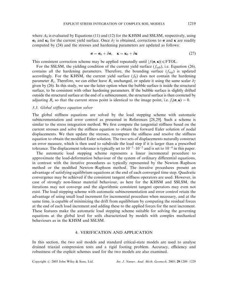
Figure 8 depicts the total number of successful subincrements used in each load increment forthe three models. As is shown, a higher resolution of the stress tolerance will always invoke alarger number of successful subincrements during each loading step for all the three models. Thenumber of the successful subincrements increases again roughly

ffiffiffiffiffi10

ptimes as the stress

tolerance is tightened by a factor of 10. As is observed from Figure 8(a) and (c), the MCCM and

Figure 6. Mesh for rigid strip footing: 288 triangular six-noded elements with 625 nodesand 1143 degrees of freedom.


J. ZHAO ET AL.1224

SSLSM do not require any subincrement initially, because of the elastic regions in the model.For the KHSM, the elastic region is very small and plastic yielding occurs very early, and thussubincrementation is required right from the beginning.

0

5

10

15

20

25

30

0 0.1 0.2 0.3 0.4 0 0.1 0.2 0.3 0.4

0 0.1 0.2 0.3 0.4

Footing Displacement/(L /2)

Fo

oti

ng

Lo

ad

MCC

SSLSM

KHSM

(a)

0

1

2

3

4

5

6


Rs

in K

HS

M

a

b c

d

(b)

0.5

0.6

0.7

0.8

0.9

1

1.1


R*

in S

SL

SM

a

b

c

d

(c)

Figure 7. The rigid footing problem analysed by the MCCM, KHSM and SSLSM: (a)footing displacement vs footing load; (b) footing displacement vs structural index Rs

evolution in KHSM at reference points; and (c) footing displacement vs structural indexRn evolution in SSLSM at reference points.

Table IV. Rigid footing on KHSM by explicit Euler substepping integration.

CPU Total successful Max. successful RelativeModel Stress tolerance time (s) subincrements subincrements stress error

MCC STOL ¼ 1:0E� 4 19 8118 17 3.890E-05STOL ¼ 1:0E� 5 19 21 019 44 9.205E-06STOL ¼ 1:0E� 6 21 61 823 120 6.845E-07STOL ¼ 1:0E� 7 31 190 824 437 }

KHSM STOL ¼ 1:0E� 4 23 28 827 71 7.860E-05STOL ¼ 1:0E� 5 24 64 101 126 1.780E-06STOL ¼ 1:0E� 6 30 178 601 244 2.729E-07STOL ¼ 1:0E� 7 48 542 249 608 }

SSLSM STOL ¼ 1:0E� 4 19 9654 18 8.200E-05STOL ¼ 1:0E� 5 19 24 589 50 5.520E-06STOL ¼ 1:0E� 6 21 68 181 154 5.783E-07STOL ¼ 1:0E� 7 37 210 311 484 }



5. CONCLUSIONS

Some key conclusions from this study are as follows.

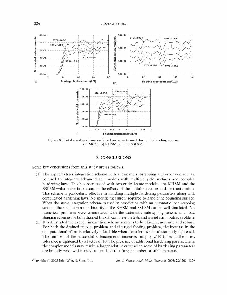
(1) The explicit stress integration scheme with automatic substepping and error control canbe used to integrate advanced soil models with multiple yield surfaces and complexhardening laws. This has been tested with two critical-state models}the KHSM and theSSLSM}that take into account the effects of the initial structure and destructuration.This scheme is particularly effective in handling multiple hardening parameters along withcomplicated hardening laws. No specific measure is required to handle the bounding surface.When the stress integration scheme is used in association with an automatic load steppingscheme, the small-strain non-linearity in the KHSM and SSLSM can be well simulated. Nonumerical problems were encountered with the automatic substepping scheme and loadstepping schemes for both drained triaxial compression tests and a rigid strip footing problem.

(2) It is illustrated the explicit integration scheme remains to be efficient, accurate and robust.For both the drained triaxial problem and the rigid footing problem, the increase in thecomputational effort is relatively affordable when the tolerance is substantially tightened.The number of the successful subincrements increases roughly

ffiffiffiffiffi10

ptimes as the stress

tolerance is tightened by a factor of 10. The presence of additional hardening parameters inthe complex models may result in larger relative error when some of hardening parametersare initially zero, which may in turn lead to a larger number of subincrements.

1.0E+00

1.0E+01

1.0E+02

1.0E+03

1.0E+04

1.0E+05

0 0.1 0.2 0.3 0.4

Footing displacement/(L/2)

Su

cces

sfu

l su

bin

crem

ents

STOL=1.0E-7

STOL=1.0E-6

STOL=1.0E-5

STOL=1.0E-4

(a)

1.0E+02

1.0E+03

1.0E+04

1.0E+05

0 0.1 0.2 0.3 0.4


Su

cces

sfu

l su

bin

crem

ents STOL=1.0E-7 STOL=1.0E-6

STOL=1.0E-5 STOL=1.0E-4

(b)

1.0E+00

1.0E+01

1.0E+02

1.0E+03

1.0E+04

1.0E+05

0 0.05 0.1 0.15 0.2 0.25 0.3 0.35 0.4


Su

cces

sfu

l su

bin

crem

ents STOL=1.0E-7

STOL=1.0E-6

STOL=1.0E-4

STOL=1.0E-5

(c)

Figure 8. Total number of successful subincrements used during the loading course:(a) MCC; (b) KHSM; and (c) SSLSM.


J. ZHAO ET AL.1226

(3) The implementation of these complex soil models into finite element codes facilitates theirapplication into boundary-value problems. Modelling of overconsolidated soils underdrained triaxial compression shows that both the KHSM and the SSLSM predict asmoother stress–strain curve than those from standard Cam-clay models. Simulation ofstructured soils under drained triaxial compression indicates that the initial structure has asignificant effect on the predictions of both the KHSM and the SSLSM. Both modelspredict that a soil with an initial structure can sustain a larger shear stress than theremoulded soil. However, to attain this by the SSLSM, special attention must be paid toensure that the initial void ratio corresponds to the initial structure. Modelling of the rigidstrip footing by the KHSM and the SSLSM illustrates that implemented complex soilmodels can be applied to solve boundary-value problems. The effects of the initialstructure on the load–displacement response are noticeable when the predictions of thesemodels are compared that of the modified Cam-clay model.

APPENDIX A

For the KHSM, the following expressions for B can be obtained:

B1 ¼p0c

ln � kn

@fb@p0

B2 ¼oð1� RsÞln � kn

ded

ðB3;B4ÞT ¼ %a

B2

Rsþ

B2

p0c

� �þ Bmðrc � rÞ

ðA1Þ

where

Bm ¼ H � n : rdp0

p0cþ %a

dRs

Rs

� �� b; n ¼

@fb@p0;@fb@q

� �T; r ¼ ðp0; qÞT

ded ¼

ffiffiffiffiffiffiffiffiffiffiffiffiffiffiffiffiffiffiffiffiffiffiffiffiffiffiffiffiffiffiffiffiffiffiffiffiffiffiffiffiffiffiffiffiffiffiffiffiffiffiffiffiffiffið1� AdÞ

@fb@p0

� �2þAd

@fb@q

� �2s; %a ¼ ðp0%a; q%aÞ

T; b ¼ n � ðrc � rÞ

rc ¼ Rsp0c þ

Rs

Rbðp0 � p0%aÞ;

Rs

Rbðq� q%aÞ

� �T; bmax ¼ 2

ðRs � RbÞRb

n � ðr� %aÞ

H ¼Bpc

ðln � knÞRb

b

bmax

� �cþHc; Hc ¼

Rsp0cfx½ðp

0 � p0%aÞ þ Rbp0c�g

ðln � knÞ ðp0 � p0%aÞ2 þ ððq� q%aÞ=M2Þ2

x ¼ ðp0 � p0%aÞ þ

oð1� RsÞRs

ded

and o; Ad; B; and c are additional model parameters.In the SSLSM, B has the following elements:

B1 ¼v*p0cl� k

@fsub@p0

; B2 ¼ �vM

l� km lnR ded; B3 ¼

vMa

l� kRnð1� RnÞ ded ðA2Þ



where

ded ¼

ffiffiffiffiffiffiffiffiffiffiffiffiffiffiffiffiffiffiffiffiffiffiffiffiffiffiffiffiffiffiffiffiffiffiffiffiffiffiffiffiffiffiffiffiffiffiffiffiffiffiffiffiffiffiffiffiffiffiffiffið1� AdÞ

@fsub@p0

� �2þAd

@fsub@q

� �2s

and m; a; and Ad are additional model parameters. l and k are the slopes of the normalcompression line and swelling line in the plane of v� ln p0; respectively.

ACKNOWLEDGEMENTS

The authors would thank Prof. David Potts for his helpful suggestions. Comments from the twoanonymous reviewers are also gratefully acknowledged.

REFERENCES

1. Roscoe KH, Schofield AN, Wroth CP. On the yielding of soils. Geotechnique 1958; 8:22–52.2. Roscoe KH, Schofield AN. Mechanical behaviour of an idealised ‘wet’ clay. Proceeding of 2nd European Conference

on Soil Mechanics and Foundation Engineering, vol. 1, Wiesbaden, 1963; 47–54.3. Schofield AN, Wroth CP. Critical State Soil Mechanics. McGraw-Hill: London, 1968.4. Roscoe KH, Burland JB. On the generalised stress–strain behaviour of ‘wet’ clay. Engineering Plasticity. Cambridge

University Press: Cambridge, 1968; 535–560.5. Carter JP, Booker JR, Wroth CP. A critical state soil model for cyclic loading. In Soil Mechanics}Transient and

Cyclic Loads, Pande GN, Zienkiewicz OC (eds). Wiley: New York, 1982; 219–252.6. Muir Wood D. Kinematic hardening model for structured soil. In Numerical Models in Geomechanics, Pande NV,

Pietruszczak S (eds). Balkema: Rotterdam, 1995; 83–88.7. Sheng DC, Sloan SW, Yu HS. Aspects of finite element implementation of critical state models. Computational

Mechanics 2000; 26:185–196.8. Liu MD, Carter JP. On the volumetric deformation of reconstituted soils. International Journal for Numerical and

Analytical Methods in Geomechanics 2000; 24:101–133.9. Rouainia M, Muir Wood D. A kinematic hardening constitutive model for natural clays with loss of structure.

Geotechnique 2000; 50(2):153–164.10. Asaoka A. Consolidation of clay and compaction of sand}an elasto-plastic description. The 12th Asian Regional

Conference on SMGE, Singapore, August 2003.11. Simo JC, Taylor RL. Consistent tangent operators for rate-independent elasto-plasticity. Computer Methods in

Applied Mechanics and Engineering 1985; 48:101–118.12. Potts DM, Gens A. A critical assessment of methods of correcting for drift from the yield surface in elastoplastic

finite element analysis. International Journal for Numerical and Analytical Methods in Geomechanics 1985; 9:149–159.13. Oritz M, Simo JC. An analysis of a new class of integration algorithms for elasto-plastic constitutive relations.

International Journal for Numerical Methods in Engineering 1986; 23:353–366.14. Britto AM, Gunn MJ. Critical State Soil Mechanics via Finite Elements. Ellis Horwood: Chichester, 1987.15. Gens A, Potts DM. Critical state models in computational geomechanics. Engineering Computations 1988; 5:

178–197.16. Borja RI, Lee SR. Cam-clay plasticity. Part I: implicit integration of elasto-plastic constitutive relations. Computer

Methods in Applied Mechanics and Engineering 1990; 78:49–72.17. Borja RI. Cam-clay plasticity. Part II: implicit integration of constitutive equations based on a non-linear elastic

stress predictor. Computer Methods in Applied Mechanics and Engineering 1991; 88:225–240.18. Jeremic B, Sture S. Implicit integration in elastoplastic geotechnics.Mechanics of Cohesive-Frictional Materials 1997;

2:165–183.19. Macari EJ, Weihe S, Arduino P. Implicit integration of elastoplastic constitutive models for frictional materials with

highly non-linear hardening functions. Mechanics of Cohesive-Frictional Materials 1997; 2:1–29.20. Borja RI, Lin CH, Montans FJ. Cam-clay plasticity. Part IV: implicit integration of anisotropic bounding surface

model with nonlinear hyperelasticity and ellipsoidal loading function. Computer Methods in Applied Mechanics andEngineering 2001; 190:3293–3323.

21. Tamagnini C, Castellanza R, Nova R. A generalized backward Euler algorithm for the numerical integration ofan isotropic hardening elastoplastic model for mechanical and chemical degradation of bonded geomaterials.International Journal for Numerical and Analytical Methods in Geomechanics 2002; 26:963–1004.


J. ZHAO ET AL.1228

22. Borja RI, Sama KM, Sanz PF. On the numerical integration of three-invariant elastoplastic constitutive models.Computer Methods in Applied Mechanics and Engineering 2003; 192:1227–1258.

23. Wissmann JW, Hauck C. Efficient elastic–plastic finite element analysis with higher order stress point algorithms.Computers and Structures 1983; 17:89–95.

24. Sloan SW. Substepping schemes for the numerical integration of elastoplastic stress–strain relations. InternationalJournal for Numerical Methods in Engineering 1987; 24:893–911.

25. Hashash YMA, Whittle AJ. Integration of the modified Cam-clay model in nonlinear finite element analysis.Computers and Geotechnics 1992; 14:59–83.

26. Sloan SW. Substepping schemes for the numerical integration of elastoplastic stress–strain relations. InternationalJournal for Numerical Methods in Engineering 1987; 24:893–911.

27. Sloan SW, Abbo AJ, Sheng DC. Refined explicit integration of elastoplastic models with automatic error control.Engineering Computations 2001; 18(1/2):121–154.

28. Abbo AJ, Sloan SW. An automatic load stepping algorithm with error control. International Journal for NumericalMethods in Engineering 1996; 39:1737–1759.

29. Sheng DC, Sloan SW. Loading stepping schemes for critical state models. International Journal for NumericalMethods in Engineering 2001; 50:67–93.

30. Luccioni LX, Pestana JM, Taylor RL. Finite element implementation of non-linear elastoplastic constitutive lawsusing local and global explicit algorithms with automatic error control. International Journal for Numerical Methodsin Engineering 2001; 50:1191–1212.

31. Potts DM, Ganendra D. An evaluation of substepping and implicit stress point algorithms. Computer Methods inApplied Mechanics and Engineering 1994; 119:341–354.

32. Crisfield MA. Nonlinear Finite Element Analysis of Solids and Structures, vol. 1: Essentials. Wiley: Chichester, 1991.33. Crisfield MA. Nonlinear Finite Element Analysis of Solids and Structures, vol. 2. Wiley: Chichester, 1997.34. Al-Tabbaa A, Muir Wood D. An experimentally based ‘bubble’ model for clay. In Proceedings of 3rd International

Conference on Numerical Models in Geomechanics NUMOG III, Pietruszczak S, Pande GN (eds). Elsevier AppliedSciences: Amsterdam, 1989; 91–99.

35. Hashiguchi K. Subloading surface model in unconventional plasticity. International Journal of Solids and Structures1989; 25:917–945.

36. Dafalias YF. Bounding surface plasticity. I: mathematical foundation and hypoelasticity. Journal of EngineeringMechanics (ASCE) 1986; 112(EM9):966–987.

37. Asaoka A, Nakano M, Noda T. Superloading yield surface concept for highly structured soil behaviour. Soils andFoundations 2000; 40(2):99–110.



explicit stress integration of complex soil...

Documents