explaining variation in child labor statisticsftp.iza.org/dp5156.pdfdiscussion paper series...
TRANSCRIPT
DI
SC
US
SI
ON
P
AP
ER
S
ER
IE
S
Forschungsinstitut zur Zukunft der ArbeitInstitute for the Study of Labor
Explaining Variation in Child Labor Statistics
IZA DP No. 5156
August 2010
Andrew DillonElena BardasiKathleen BeeglePieter Serneels

Explaining Variation in Child Labor Statistics
Andrew Dillon International Food Policy Research Institute
Elena Bardasi
World Bank
Kathleen Beegle World Bank and IZA
Pieter Serneels
University of East Anglia and IZA
Discussion Paper No. 5156 August 2010
IZA
P.O. Box 7240 53072 Bonn
Germany
Phone: +49-228-3894-0 Fax: +49-228-3894-180
E-mail: [email protected]
Any opinions expressed here are those of the author(s) and not those of IZA. Research published in this series may include views on policy, but the institute itself takes no institutional policy positions. The Institute for the Study of Labor (IZA) in Bonn is a local and virtual international research center and a place of communication between science, politics and business. IZA is an independent nonprofit organization supported by Deutsche Post Foundation. The center is associated with the University of Bonn and offers a stimulating research environment through its international network, workshops and conferences, data service, project support, research visits and doctoral program. IZA engages in (i) original and internationally competitive research in all fields of labor economics, (ii) development of policy concepts, and (iii) dissemination of research results and concepts to the interested public. IZA Discussion Papers often represent preliminary work and are circulated to encourage discussion. Citation of such a paper should account for its provisional character. A revised version may be available directly from the author.

IZA Discussion Paper No. 5156 August 2010
ABSTRACT
Explaining Variation in Child Labor Statistics* Child labor statistics are critical for assessing the extent and nature of child labor activities in developing countries. In practice, widespread variation exists in how child labor is measured. Questionnaire modules vary across countries and within countries over time along several dimensions, including respondent type and the structure of the questionnaire. Little is known about the effect of these differences on child labor statistics. This paper presents the results from a randomized survey experiment in Tanzania focusing on two survey aspects: different questionnaire design to classify children work and proxy response versus self-reporting. Use of a short module compared with a more detailed questionnaire has a statistically significant effect, especially on child labor force participation rates, and, to a lesser extent, on working hours. Proxy reports do not differ significantly from a child’s self-report. Further analysis demonstrates that survey design choices affect the coefficient estimates of some determinants of child labor in a child labor supply equation. The results suggest that low-cost changes to questionnaire design to clarify the concept of work for respondents can improve the data collected. JEL Classification: J21, C81, C93 Keywords: child labor, survey design, Tanzania Corresponding author: Andrew Dillon International Food Policy Research Institute 2033 K Street, NW Washington, DC 20006-1002 USA E-mail: [email protected]
* We would like to thank Economic Development Initiatives, especially Joachim de Weerdt, the supervisory staff, enumerators and data entry teams for thorough work in the field. We also appreciate the thoughtful comments by three anonymous referees and the suggestions of the Editor, which improved the paper substantially. We thank the seminar participants at IZA Workshop on Child Labor and at the Conference “Survey Design and Measurement in Development Economics”, sponsored by the World Bank, the Enterprise Initiative, and Yale University for their comments and feedback. This work was supported by the World Bank Research Support Budget and the Gender Action Plan at PREM-Gender. All views are those of the authors and do not reflect the views of The World Bank or its member countries.

2
1. Introduction and background
In the past decade, special attention has been paid to generating empirical evidence on
child labor for developing countries. Edmonds (2009) illustrates the boom in studies
on child labor and provides an overview of labor force participation rates across a
large number of countries. Recognizing the importance of both the definition of child
labor and its measurement, the International Labor Organization/IPEC’s Statistical
Information and Monitoring Programme on Child Labour (SIMPOC) has focused on
establishing standardized methods for survey design to measure children’s work (see
ILO, 2008, and ILO, 2004). Despite these efforts, there is still substantial variation in
how child labor is measured. Partly this reflects the practice of measuring child labor
as part of a broader survey, a consequence of the limited capacity of statistical offices
in low-income countries to field frequent stand-alone child labor surveys. In turn,
there can be considerable inconsistency in statistics.
Guarcello et al. (2009) carefully document the apparent inconsistency of child labor
statistics from large-scale national surveys for several countries. In Ghana, for
instance, a comparison between the Core Welfare Indicator Survey (CWIQ) (2003)
and the SIMPOC survey (2000) shows a decline in child labor of 27 percentage points
from 34 percent of children working in the SIMPOC survey. In Kenya, the Multiple
Indicator Cluster Survey 2 (MICS2 2000) and SIMPOC (1998/99) surveys report an
increase in child labor of 36 percentage points from 8 percent in the SIMPOC survey.
Changes in child labor force participation rates over time certainly could reflect real
changes – such as rapid economic growth. In this case, we would likely expect to see
similar changes in school enrollment, which Guarcello et al. (2009) do not observe.
Other explanations for such large fluctuations between two independent surveys
administered in close proximity are survey design and sample design. However,
Guarcello et al. (2009) find that differences in survey design (including questionnaire
type and fieldwork season) explain only some of the variation in child labor estimates
across surveys and that samples look otherwise comparable (including age, sex, and
urban composition). A sizeable portion of the variation in child labor statistics
remains unexplained. There is scant evidence on the impact of survey design on child
labor statistics, in contrast with adult labor, where there is more evidence, especially

3
from the United States.1 One exception is Dillon (2010), who compares two different
child labor modules within the same survey, one a standard set of labor questions that
collects information on participation and hours across various activities posed to
parents about their children, and another subjective game played by children that
reveals the distribution of their time. Comparisons between the two modules suggest
that adults report lower hours of child labor when using a standard labor module
relative to children who play the subjective game, but the paper cannot disentangle the
proxy effect versus the effect of question type/design.
The objective of this paper is to explore further what aspects of survey design affect
child labor indicators to assess these tradeoffs. We focus on two main areas: the effect
of including screening questions to structure the questionnaire regarding labor market
activities and the respondent type. The sequencing of employment questions is posited
to have a large influence on labor statistics. This may be particularly relevant in a
setting where a significant proportion of individuals are employed in household
enterprises or home production and are not directly remunerated in the form of a
salary or wage. Classification of activities between those that are considered “work”
and those that are not may induce confusion in survey respondents who are not
familiar with internationally recognized definitions of labor market activities and may
have a very personal concept of “employment.” For example, the stand-alone question
“Did you work in the last 7 days?” is hypothesized to systematically undercount
persons who work in household enterprise activities without direct wage payments,
e.g., unpaid family workers or women (Anker, 1983), who may not recognize
themselves (or be recognized by other household members) as “employed
individuals.” This type of employment question may also be flawed for measuring
child labor, especially when children participate in economic activities related to the
household enterprise or home production, and even more so when such activities are
seasonal, occasional, or occupy only a few hours a week. This is especially the case in
developing countries.
Respondent type may also influence the labor statistics generated. Borgers et al.
(2000) illustrate that, given the appropriate question structuring and interview
1 Bardasi et al. (2010) review some of the literature with a focus on evidence from low-income settings.
4
conditions, children older than 10 years of age have sufficient cognitive development
to respond accurately to survey questions. However, in practice other household
members are often asked to report on the children’s activities, rather than the child
him or herself. In related work on adults, we find that the effect of proxy response has
a large and statistically significant effect on a number of labor statistics, like labor
force participation, weekly hours worked, and daily earnings (Bardasi et al., 2010).
We also find that the relationship between the proxy and the respondent, with respect
to age, education, and gender, influences the estimated adult labor statistics.
Focusing on children age 10-15, we assess the implications of survey methods both on
average and in relation to the characteristics of the child and his/her household. We
draw lessons for measuring child labor force participation, the type and intensity of
child work (particularly work that occurs in household enterprises and farms), and the
changes in patterns of child work over time. The setting for this work, Tanzania,
influences the extent to which these findings might be applicable to other countries.
Specifically, we are testing alternative survey designs in a context that we
characterize, based on our field experiences, as one where there are not negative
perceptions of child labor (see discussion in Bass, 2004, who draws a similar
conclusion about perceptions of child labor in Sub-Saharan Africa). Thus, we are not
testing whether households try to deny or hide child labor activities and whether
specific questionnaire designs can circumvent this problem, but we are assuming—
quite confidently—that this problem is marginal in our setting.
In this study, we focus on child labor data from household surveys. Household-based
surveys are unlikely to be appropriate sources of data on the most hazardous or worst
forms of child labor, which are rare in Tanzania. Such measures should ideally be
collected through other methods (see ILO, 2008). Our intent is to measure the extent
to which children are engaged in productive activities, which is a first step in the
measurement of child labor—not testing how to measure child labor according to the
ILO statistical definition.
The structure of the paper is as follows. We describe the experimental design and the
identification strategy to test differences in questionnaire design and respondent type

5
in the next section. Section 3 provides a description of the data collected; Section 4
presents our results. Section 5 concludes.
2. The survey experiment Whether changes in the measurement method have an effect on the statistics they
produce is, ultimately, an empirical question. We designed and implemented a survey
experiment in Tanzania focusing on two key dimensions of labor survey design: the
inclusion of screening questions in the questionnaire with respect to identifying labor
force participants and the type of respondent. In this experiment, we have two
different questionnaire designs (which we call “detailed” and “short”) and two
respondent types (proxy and self-report). Households were randomly selected for the
survey from seven districts in Tanzania; we describe the household selection process
in the subsequent section. After households were selected within the village, they
were randomly assigned to one of four groups defined by the combination of the two
experiments, one orthogonal to the other: detailed and self-report, detailed and proxy,
short and self-report, and short and proxy. Details on the sampling approach and
survey assignment for households and individuals are provided in Section 4.
The experiment was conducted for both adults and children—individuals eligible for
data collection were all those age 10 and older. In this paper, we focus on the
responses from children and the measurement of child labor. We define child labor as
the labor force activity of a child ages 10 to 15 who has engaged in at least one hour
of labor market activity over the past seven days. An internationally recognized
definition of child labor remains an open item in the child labor policy agenda as
current international agreements such as the ILO’s Convention 138 agree on age
limits for child labor, but leave discretion to member countries on hours and activity
restrictions in defining child labor. Our definition is consistent with the ILO’s
Statistical Information and Monitoring Program on Child Labor (SIMPOC) definition
of child labor.2
2 In another paper, we focus on the measurement of labor statistics for all the adult population (Bardasi et al., 2010). Note that the “adult labor statistics experiment” and the “child labor statistics experiment” on which we report in this paper are not separate experiments, but rather focus on two different populations in the same survey experiment.

6
For the first dimension of this survey experiment, we have a “detailed” labor module
and a “short” labor module. The short module reflects the approach commonly used in
short questionnaires, such as the Core Welfare Indicator Survey (CWIQ). This short
module is often used to generate statistics with a high frequency, for example with
annual regularity, in lieu of multi-topic household surveys that are too demanding to
implement on an annual basis. In our survey experiment, the detailed module differs
from the short module in two ways: the set of screening questions is longer in the
detailed module and the detailed module collects information on second and third
jobs. Our objective is to compare the impact of the different screening questions. The
detailed module includes several screening questions about labor force participation,
specifically, whether the person has worked for someone outside the household (as an
employee), whether s/he has worked on the household farm, and whether s/he has
worked in a non-farm household enterprise (three separate yes/no questions). These
questions are asked with respect to the past 7 days as well as for the past 12 months.
In the short module, there is only one question for each of the two reference periods,
namely whether s/he has worked in the past 7 days (or past 12 months, respectively).
From these screening questions (yes to any of the three in the detailed module; a yes
to the one question in the short module), a person is identified working (employed). In
the remainder of the paper, we focus on employment statistics with respect to the past
7 days of a worker’s main job. Although we expect different results depending on the
reference period (seasonal activities are likely to be particularly important in the
measurement of child labor), we decided to focus on the past 7 days because this is
the standard ILO approach in measuring employment. Moreover, our survey was
carried out over a whole year, so seasonality effects should average out between
survey assignments. In both the detailed and short versions, the employed are then
asked their occupation, sector, employer, hours, and wage. There are too few second
and third jobs in the data to analyze those data (6 children and 1 child report a second
and third job, respectively).
In the second dimension of the experiment, we vary the respondent to whom the
questions are asked: directly to the child or to a proxy respondent. Response by proxy
rather than self-report is a common practice in household surveys, with the household
head often answering all questions. The ILO guidelines for child labor statistics are
that these questions be answered by the child, without proxy, and in cases where
7
young children (less than 9 years) have difficulty comprehending or responding to
questions, someone else in the family, usually the mother or elder sister, may assist
them (ILO, 2004). Although self-reporting (for respondents of some minimum age,
typically 10 years or older) is the established standard for multi-topic household
surveys (Schaffner, 2000), in practice proxy respondents are often used when
individuals are away from the household working or otherwise unavailable to
interview in the time allotted in an enumeration area to conduct interviews. In our
survey experiment, the proxy respondent is randomly chosen from among the
household members who are at least 15 years old. This age threshold reflects common
practice in fieldwork as it is unlikely for an enumerator to choose another child
(younger than 15) to be a proxy respondent for children (or adults) in the household.
The proxy respondent is thus either the head of household, spouse of the head, or an
older child or relative living in the household.3 The proxy respondent then reports on
two other household members who are at least 10 years old. In practice, proxy
respondents are usually not randomly chosen but selected on the basis of availability
and knowledge of the person for whom they will respond. Although, in this sense, the
experiment does not exactly mimic the actual conditions of proxy respondents, the
randomization of proxies allows us to investigate whether proxy characteristics may
have an effect on the statistics generated.
Tables A1 and A2 in the Annex report the key employment questions in the short and
detailed questionnaires and summarize the main features of the two experiments. The
full English versions of the labor modules are presented in Bardasi et al. (2010).
Combining each of the above two dimensions in our experiment gives rise to a 2 x 2
randomized design that reflects commonly used approaches in practice: a detailed
questionnaire with self-respondents, a detailed questionnaire with proxy respondents,
a short questionnaire with self respondents, and a short questionnaire with proxy
respondents. We use the results from the detailed self-report questionnaire as the
benchmark reference for our analysis. This is generally considered to be the “best
practice” approach of household surveys. It corresponds to ILO recommendations,
which prescribe a detailed questionnaire with children self-reporting, as well as
3 The Tanzanian CWIQ 2006 data indicate that the average Tanzanian household has between two and three adults who could serve as a proxy.

8
recommendations of the World Bank. However, it is not possible to establish with our
experiment that the detailed self-report questionnaire (or any other alternative for that
matter) is the “gold standard,” or the “best” approach to collect child labor statistics.
Instead, we will be able to document variations across survey design and identify the
most important dimensions along which variations occur.
In each of the four designs, in addition to the labor module, the questionnaire also
includes five other modules: a household roster, and sections on household assets,
dwelling characteristics, land, and consumption expenditures. The questions in these
sections follow the same sequence and phrasing, and refer to the same recall periods
in the detailed and short questionnaires. The labor module was administered before
the consumption module, but after the land module in the questionnaire.
Before analyzing the child labor statistics, we first compare household and individual
level variables across the assignments to ensure that characteristics are not statistically
different on average. From an analytical perspective, we have organized the analysis
to address two types of questions: (i) the effects of the change in survey design on
child labor statistics, and (ii) whether survey design affects the relationship between
child labor and the variables of interest that are typically documented in the empirical
literature as being important covariates of child labor. Regardless of whether
variations in child employment are found on average, it is possible that the survey
design affects reporting on child labor in a non-random way with respect to those
characteristics that are generally found to explain (or be correlated with) child labor.
To address the first question, we follow two steps. We first estimate differences in
mean child labor statistics across assignments.4 We compare the mean outcomes in
children’s labor force participation, occupation, daily hours worked, and weekly
earnings across the four groups for the child’s main job. Since the survey assignments
4 In the parlance of randomized control design, to estimate the average treatment effect, we ideally want to estimate ∆ = Yt
1-Y t0 which is the difference of the outcome variable of interest at time t
between two treatments denoted by the superscripts 1 and 0. However, since ∆ is unobservable to the econometrician because a household does not receive two treatments simultaneously, one estimates the treatment effect given the observable data, i.e. TE = E (Yt
1 | T=1) - E (Yt0 | T=0). Since in a properly
implemented randomized design, the treatment and control groups have identical characteristics on average because the groups were composed of randomly allocated households, differing only with respect to the treatment received, the selection bias, E (Yt
0 | T=1) - E (Yt0 | T=0), equals zero and the
estimate of the treatment effect is unbiased.
9
are randomly allocated, we abstract from unobserved heterogeneity in individual,
household, or village characteristics.
In a second step, we formally estimate the marginal survey design effects using the
following specification:
yi = α + βPPh + βSSh + λXi + γDh + ɛh
(Eq. 1)
Where iy are the different labor statistics (such as labor force participation, labor
supply, earnings, and occupational choice) for the i th child, Ph is an indicator variable
for the proxy treatment of children in household h, Sh is an indicator variable for the
short questionnaire treatment of children in household h, Xi is a vector of child and
household characteristics for the i th individual, D captures district indicators, and ɛ is
the stochastic error term, which is randomly distributed across households.
Survey data are also used to estimate behavioral equations, for example how the age
of the child and other personal and household characteristics impact the probability of
the child working. We investigate whether point estimates of key covariates (vector
Z) in these equations vary when different survey designs are used, focusing on four
important covariates of child work, as identified by seminal papers in the child labor
literature: the child’s age (Edmonds, 2009), household size (Edmonds, 2005),
household assets (Basu and Van, 1998), and household land size (Bhalotra and
Heady, 2003). To do this, we interact the survey assignment variables with each of
these variables minus its mean value in the sample (Zi – mean Z), while controlling for
the survey assignment effects, the covariate of interest, household and individual
characteristics (Xi, which includes Z variables), as well as district indicators. We
estimate the following specification:
yi = α + βPPh + βPPh(Zi – mean Z) + βSSh + βPSh(Zi – mean Z)
+ λXi + γDh + ɛh (Eq. 2)
10
3. The data
The survey experiment, the Survey of Household Welfare and Labour in Tanzania
(SHWALITA), was implemented in Tanzania. The work was implemented by a well-
established data collection enterprise, Economic Development Initiatives (EDI) with
the capacity to undertake high-quality field studies. The survey assignments were
carefully piloted in a rural and an urban area not part of the sample. A qualitative
debriefing with the field supervisors took place at the end of each day during the pilot,
in order to solicit their feedback on a range of issues.5 In addition, a subset of
households was selected for qualitative interviews with the respondents, in order to
see whether wording and structure of the questionnaire could be further improved.6
Training manuals and enumerator instructions were then revised based on these
sources of feedback during the pilot. Enumerators were then trained and the survey
was implemented.7
SHWALITA was purposively designed and fielded to study the implications of the
alternative survey designs for employment indicators and consumption expenditure
measures. Here we focus on the component that applies to employment indicators.
The field work was conducted from September 2007 for 12 months in villages and
urban areas from 7 districts across Tanzania: one district in the regions of Dodoma,
Pwani, Dar es Salaam, Manyara, and Shinyanga region, and two districts in the
Kagera region. Households were randomly drawn from a listing of all households in
5 The feedback focused on nine areas: 1. General impressions of the respondent’s comprehension; 2. Question phrasing; 3. Question sequencing; 4. Completeness of lists of question responses; 5. Clarity of interviewer instructions; 6. Completeness of interviewer manual to resolve field problems encountered; 7. Questions that should be restructured for greater clarity and respondent comprehension; 8. Conceptual or cultural difficulties in translating questions to local language; 9. Areas of emphasis for training enumerators. One of the most important parts of the questionnaire to pilot was the selection of proxy and self-reporting respondents. After a day of training, interviewers spent significant time practicing with examples. 6 During this qualitative interview, respondents were asked open-ended questions to solicit how they thought about the survey questions, why they chose the responses they did, and how they thought about concepts such as work, household production, and their primary activities. 7 The enumerators were trained with the assistance of field supervisors who undertook the questionnaire pre-testing exercise. The training consisted of explaining the research objectives of the survey as well as the “sense” of each question, reinforcing the standards required for correct completion of the household questionnaire and the working relationship between enumerator and supervisor. A field experience to practice administering the questionnaire was part of the training. An interviewer manual was prepared to provide specific guidance during the training period, and to serve as a reference during the implementation. Throughout the training, special emphasis was put on standardization of the manner in which questions are posed and the correct selection of proxy and self-reporting respondents using a random number list.
11
the village or urban enumeration area and randomly assigned to one of the four groups
defined by the two experiments. The total sample is 1,344 households (with two of
these households being replacement households for refusals to participate), with 336
households assigned to each of the four labor modules. Although the sample of 1,344
is not designed to be nationally representative of Tanzania, the districts were selected
to capture variation in Tanzania—both urban/rural as well as along other socio-
economic dimensions. The basic characteristics of the SHWALITA households
generally match nationally representative data from the Household Budget Survey
(2006/07) (results not presented here). Households were interviewed over 12 months,
but because of small samples we do not explore the variations across main seasons
(such as the harvest season with peak labor demand and the dry seasons with low
demand).
After the households were randomly selected and randomly assigned to one of the
four assignment groups, respondents and proxies were selected according to the
following rules. In households assigned to self-report, up to two individuals ages 10
and older were randomly selected to self-report. In households assigned to proxy
report, one household member over 15 years was first selected to proxy report; in a
second stage, up to two household members age 10 and older (after excluding the
individual chosen to be a proxy respondent) were selected to be reported on by the
proxy. The proxy also reported for him/herself, and was considered a self-report in
this case. Random selection was conducted by first listing eligible individuals (either
proxies or self-reports). Then the enumerator examined a random number table pre-
printed in the questionnaire that had random numbers generated and listed in columns
that corresponded to the potential total number of eligible individuals that could be
listed. Each of these tables was generated uniquely for each questionnaire and for
each set of listing exercises (either proxies or self-reports) that were required of the
enumerator.
Because eligible respondents were all those age 10 and older, the sample selected for
our analysis included both adults and children. In this paper, we limit our sample to
the sub-group of children. Of the total sample of 1,344 households, 494 had at least
one child age 10-15 years, resulting in a sample of 566 children. We focus on the
subset of households in which these children reside. Some main characteristics of

12
these households are presented in Table 1 by survey assignment. To verify the random
nature of the assignment of households to one of the four survey types, we test
whether the different household characteristics differ across the four assignment
groups. We do this by regressing each characteristic on three indicator variables that
reflect the survey assignment (the fourth group being the base category) and test for
joint significance of the coefficients using an F test. For most household
characteristics, the difference is insignificant, reflecting the random assignment
during the field work. Only in three cases do we observe a significant difference
between groups, indicating that households assigned to the detailed self-report and
short proxy surveys turn out to be slightly larger and own slightly more land than the
other two groups.
Turning to the 566 children, we classify them on the basis of the survey assignment
they receive. This is the combination of the module assigned to the household and
sub-household assignment of the child. Children were randomly selected from among
all members age 10 and older to self-report or be reported on by proxy. In three cases,
children selected to self-report were unavailable and their labor information was
collected by proxy respondent. Omitting these children, rather than reclassifying them
to their actual assignment as we have done in our analysis, has no effect on the results
presented below.
To test the random nature of the assignment, we follow the same approach as for
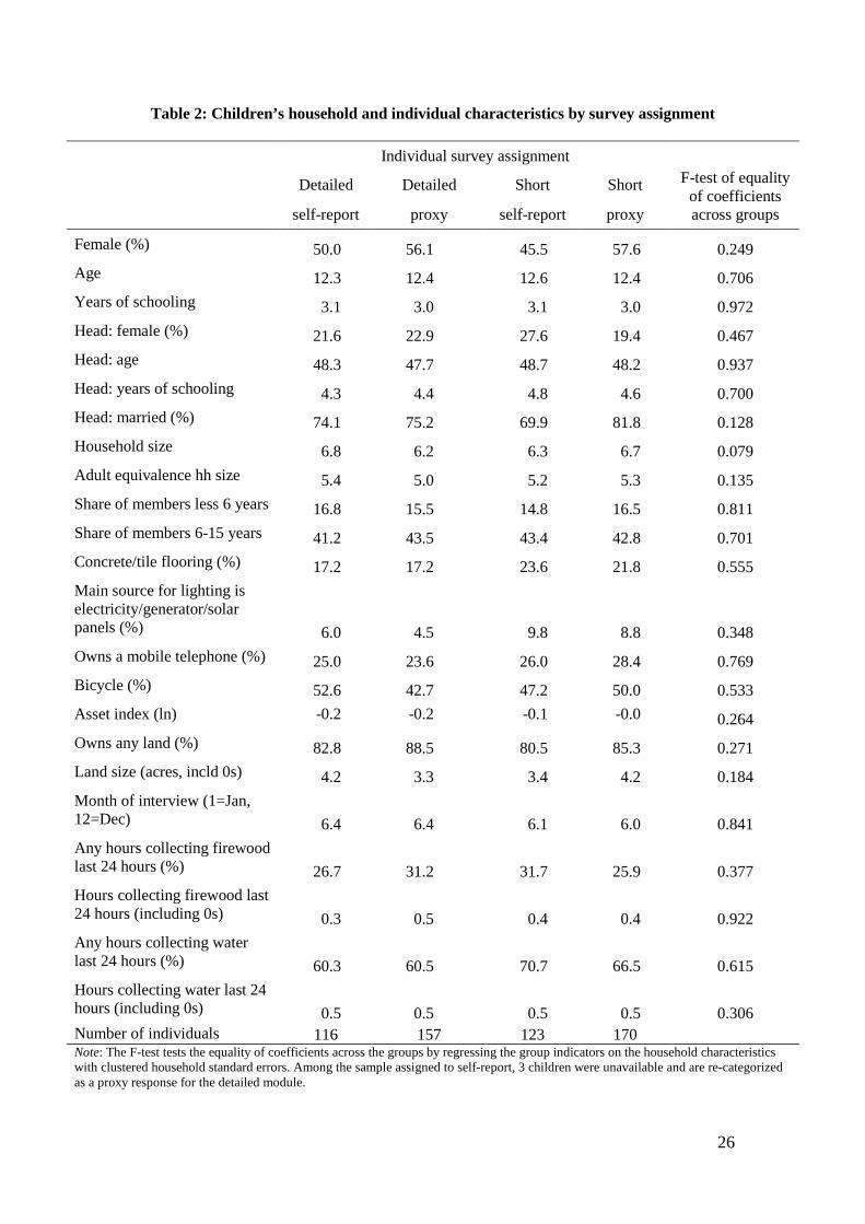
households. The results, reported in Table 2, show that we find no difference across
the four assignments, except for household size, with the households assigned to the
detailed self-report and short proxy surveys slightly larger. Consistent with the design
of the survey experiment, there are more households with proxy reported children
(Table 1 columns 2 and 4) and more individual children who are proxy reported
(Table 2 columns 2 and 4). This is because proxy respondents can only be adults age
15 years and older. Thus, in households selected to the proxy assignment, children age
10-14 have a higher probability of being selected to be proxy subjects than to be self-
reports, compared with children in households selected to the self-report assignment.
4. Results
13
We present the results in three parts. In the first part, we examine differences across
the children for three key statistics: their labor force participation (LFP) rate, their
weekly hours of labor supply, and their main activity in their main job. We also
consider time-use statistics focusing on two household chores that are often carried
out by children: the collection of firewood and water.8 These time-use questions are
identical across the four survey designs and are asked to all children regardless of
their employment status, with the only survey design variation arising from the
respondent type (self-report or proxy). Throughout we focus on a comparison between
the results generated by the short and detailed modules and a comparison between
those generated by the proxy and self-reported modules.
In the second part, we estimate the average effects of survey type for each of these
statistics using standard analysis (probit, OLS, and multinomial logit) where LFP,
weekly hours, and main activity are in turn left-hand-side variables, and the survey
assignment as well as household and individual characteristics and district effects are
right-hand-side variables, as set out in Equation 1.
In the third part, we estimate Equation 2 to investigate whether the effects on child
labor of the personal and household characteristics commonly analyzed in the child
labor literature are sensitive to changes in the survey type.
Differences in labor indicators across survey type
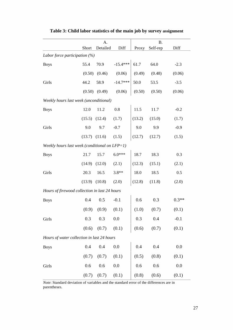
Table 3 present differences in LFP, working hours, and time spent on firewood and
water collection by questionnaire and respondent type, disaggregated by gender. In
each case, we test for a difference in means across survey type groups using a t-test.
Row 1 of Table 3, for instance, first reports the mean LFP of boys obtained from the
short module (55.4 percent) and compares this with the mean LFP for boys obtained
from the detailed module (70.9 percent) and tests whether the difference (-15.4
percentage points) is statistically different from zero. Following the conventional
definition, domestic activities (cleaning house and cooking) are not considered
8 Collecting firewood and water are activities that are included in the System of National Accounts definition of economic activities and should in principle be defined as “work,” although in practice they are routinely excluded.

14
economic activities and are not included in LFP. Note that when comparing means
between two survey designs (e.g., detailed vs. short questionnaire), we are “pooling”
statistics with respect to the other experiment (e.g., self-report vs. proxy).9
We find that there are significant differences in reported LFP for boys and girls when
using the short module compared with the detailed module. LFP with the short
module is 15 percentage points lower for both groups. The difference between the
proxy and self-reported statistic, however, is not statistically significant for either
boys or girls (the difference is -2.3 and -3.5 percentage points, respectively).
One reason why we may observe large differences in LFP between the short and
detailed modules is the under-reporting of marginal jobs (i.e., jobs that are especially
short, in terms of weekly hours) in the short module. If this is the case, we expect to
observe longer average weekly hours conditional on working for the short than the
detailed questionnaire, while average weekly hours for the whole sample (i.e.,
including the zeros) may not differ substantially between the two experiments. This is
exactly what we observe, which suggests that when using the short questionnaire,
marginal jobs are disproportionately under-reported compared with jobs with longer
weekly hours in comparison to what is reported by the detailed questionnaire.
Reported time spent on the collection of firewood and water is generally not
statistically different across groups, with one exception: boys are reported to spend
more time on collecting firewood when reported by proxy.
Of particular interest is to assess whether the relationship of the proxy to the child,
particularly that of the child to his/her parents, may influence labor statistics. As
proxy assignment was random among the eligible respondents in the household who
were at least 15 years old, no biases due to the selection of proxy should be present in
our estimates. Parents of the child make up 67.5 percent of the proxy responses.
Grandparents account for 10.4 percent of proxy responses, while siblings report on
9 The intent of the survey experiment was not to generate statistics on child labor for comparison with other surveys in Tanzania, where there will be differences in questionnaire design as well as samples and field supervision. Nonetheless, we note that our LFP rates are higher than the 46 percent LFP reported by Guarcello et al. (2009), perhaps in part driven by a large share of rural households in our sample.
15
their own sibling in 14.2 percent of the cases.10 Restricting the proxy sample to only
the sub-sample of parental proxies does not significantly change the estimates for
proxy-reported statistics in Table 3 or the regression results in Table 5 discussed
below. Fathers as proxy respondents report lower LFP and higher working hours of
their children than do mothers, but the difference is not statistically significant. These
results are available upon request.
In Table 4, we turn to the distribution of children’s main activities across broadly
defined categories. Participation in domestic duties, while not included in labor force
statistics, is commonly collected, particularly in a child labor context. This is usually
done by including domestic duties as a possible answer to the questions regarding the
individual’s main activity. Here we examine how reporting on domestic duties
changes when using one overall question about any work (short module) compared
with using three screening questions that require the respondent to specify wage work,
farm work, and non-farm household enterprise work (detailed module). For the short
module, the distribution across main categories is derived from a single question
(question 4 in the short module – see Table A1, first column); for the detailed module,
it is derived from question 9 (see Table A1, second column). The results in Table 4
show that the difference in questionnaire design between the short and detailed
modules has a large and statistically significant impact on reports for both boys and
girls. The first interesting finding is that the short questionnaire generates lower
percentages of “no work” answers than the detailed questionnaire, i.e., higher
percentages of individuals who classify themselves in employment.11 The difference
is especially large (-20.6 percentage points) and statistically significant for girls but
not for boys. However, when asked about the sector of main activity, an extremely
large percentage of children who define themselves as “working” in the short
questionnaire indicate that they are engaged in domestic duties – the difference with
the detailed questionnaire is very large and significant for both boys (+21 percentage
points) and girls (+35 percentage points). The detailed questionnaire, by contrast,
generates higher participation in agriculture for both boys and girls (the difference
compared with the short questionnaire is about 15-16 percentage points). As for the
10 Other categories of proxies include nieces/nephews (3.5 percent), other relatives (3.2 percent), and brothers or sisters-in-law (1.2 percent). 11 In the short questionnaire, “no work” corresponds to those who answer “no” to question 1 (see Table A1, column 1); in the detailed questionnaire ‘no work’ are those who answer ‘no’ to all questions 1,3,5.
16
type of respondent, there is almost no difference between the statistics generated by
self and proxy (except for slightly fewer boys working in “other sectors”).12
Together this suggests that the additional questions contained in the detailed version
work as “screening questions,” filtering out at least part of the children that equate
domestic duties with employment. It appears that individuals who would classify
themselves as “working in domestic duties” if assigned the short questionnaire are
“screened out” when using a detailed module and end up classified as “no work.” This
most frequently happens for girls. At the same time, a non-negligible proportion of
children that would classify themselves as mainly engaged in domestic duties in the
short questionnaire are classified in agricultural activities in the detailed
questionnaire.
Regression results: Survey assignment effects
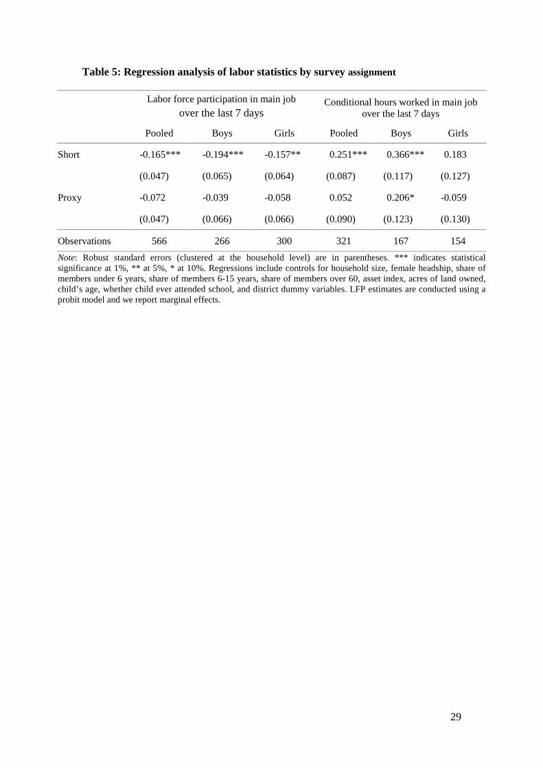
To obtain the marginal effect of each survey assignment, we estimate Equation 1
controlling for individual characteristics (age, gender, and education [highest grade
attended]), household characteristics (household size, composition, asset holdings,13
and land holdings), and district indicators. In each case, we include separate indicator
variables for the short module and the proxy module. Including an additional indicator
variable for the short proxy interaction yields very similar results (results not
presented). The results for child LFP, obtained by using a probit model, are reported
in the first columns of Table 5, and indicate that the short module yields 19
percentage points lower participation rates for boys and 16 percentage points lower
for girls (note that this is after re-classifying all domestic duties into “no work,”
following the ILO definition of employment). The use of proxy respondents also
produces underestimation of child labor with respect to self-reporting, but the effects
are much smaller (although, again, larger for girls) and not statistically significant for
our sample size. These effects are large and their variation is consistent with the
widespread differences in child labor statistics noted by Guarcello et al. (2009), who,
12 The non-agricultural sectors were: mining/quarrying/manufacturing/processing, gas/water/electricity, construction, transport, buying and selling, personal services, education/health, and public administration. Only 9 children did work in these sectors in the past 7 days. 13 The household asset index is constructed from a list of 14 durable assets, 7 livestock categories, and 7 housing characteristics. It has mean value 0.11 and standard deviation 0.9.

17
using data for four African countries (Togo, Lesotho, Burkina Faso, and Ghana), find
that a CWIQ survey, which is similar to our short questionnaire, generates lower LFP
estimates than a more detailed survey. However, since the surveys they compare are
implemented two years apart, their results are only indicative.
The right-hand-side panel of Table 5 reports the OLS results for the natural log of
weekly hours of work in the child’s main job conditional on working. The weekly
hours of work are significantly higher for boys in the short questionnaire; they are
also higher for girls, but the difference is not significant. This is consistent with the
hypothesis that in the short questionnaire marginal jobs are disproportionately more
likely to be forgotten (or not considered as jobs worth reporting) than jobs with
greater weekly hours in comparison with jobs reported in the detailed questionnaire.
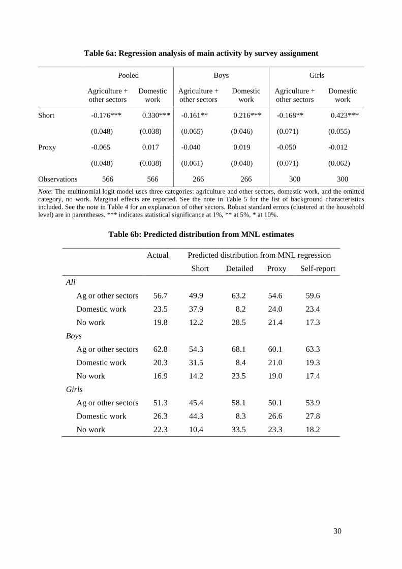
Next we estimate a multinomial logit to investigate how the survey assignment affects
the allocation across three categories (“outcomes”): agriculture and other sectors,
domestic work, and the omitted category “no work.”14 The results in Table 6a present
the marginal effects, while Table 6b presents the predicted probabilities estimated at
the mean value of the covariates for the three outcomes and the two experiments. For
the pooled sample (Table 6a, panel A), using a short module produces lower
participation in agriculture and other non-agricultural sectors with respect to “no
work” than a detailed questionnaire produces, with a larger effect for girls. Both girls
and boys are more likely to be classified as working in domestic work than identified
as not working when given a short module. This effect is also larger for girls than
boys. The proxy module is not associated with significant changes in sector
classification.
The multivariate analysis confirms that the largest difference between the short and
the detailed modules is in the allocation of children across the two categories
“domestic work” and “no work” (both considered as not in employment, based on the
ILO definition). Although the detailed module captures higher participation in
employment, the largest and most significant switch is from domestic work (in the
short module) to agriculture or no work (in the detailed module). However, the type of
14 We merged “other sectors” with the agricultural sector because there are few observations in the non- agricultural sectors. Alternative categorizations do not change the results.
18
respondent does not appear to produce large impacts on labor force participation and
the allocation across employment categories. Using proxy respondents produces
similar statistics as when asking the child directly.
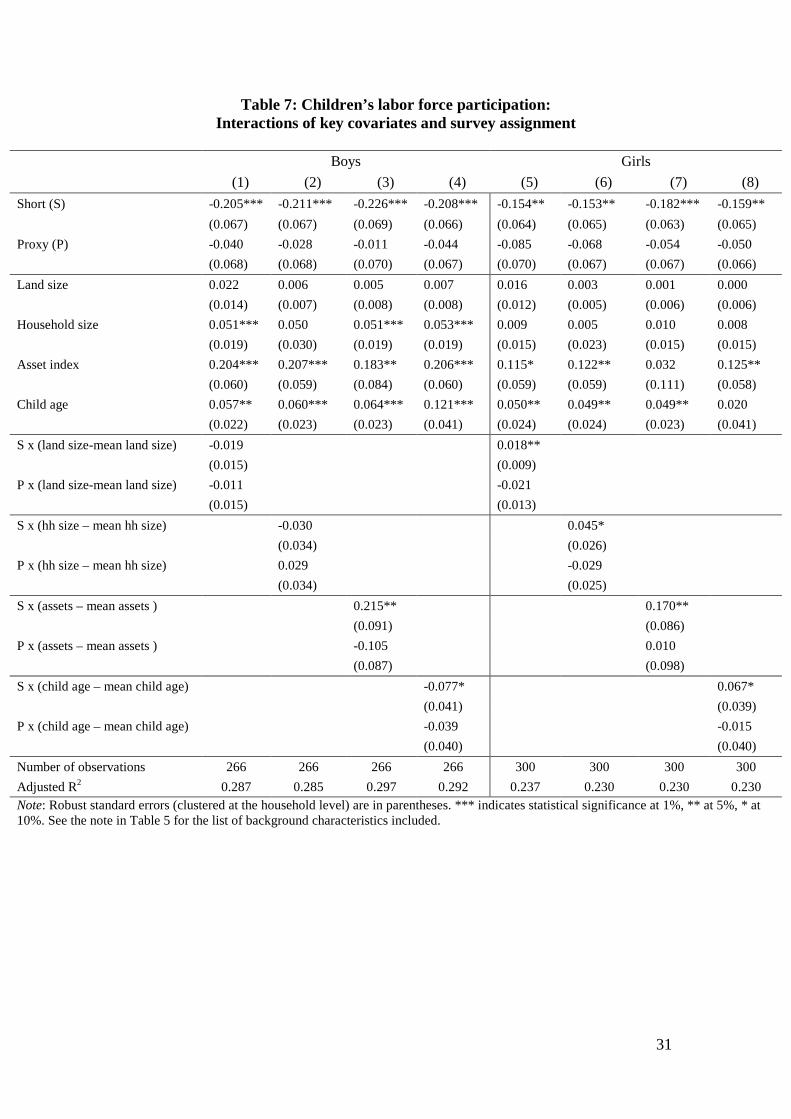
Regression results: Interaction between survey assignment and covariates
To address questions about the effect of survey methods on the estimated coefficients
of child labor determinants, we assess the relationships between child labor supply
and four variables discussed in Section 3that have been identified in the literature as
key covariates.15 All four covariates are expected, and have been observed, to be
positively related to child labor. In the subsequent discussion, we assess whether and
how the estimated coefficients that reflect these respective relationships are affected
by variations in questionnaire and respondent type.
Table 7 reports the results of estimating Equation 2 for LFP using a probit
regression.16 Columns 1-4 (5-8) present the interactions of survey types and one of the
four covariates of interest for boys (girls). The results suggest potentially important
impacts of the survey design on the estimated coefficients. For boys there are no
differential effects of survey assignment by land holdings or household size. The
negative impact of the short module is strongly attenuated for boys in households with
higher asset holdings. Conversely, the impact of the short module is greater for boys
who are older. For girls, we estimate variations in the short versus detailed impact
associated with each of the four variables of interest. The difference in LFP between
the short and detailed module is smaller for girls in households with larger land
holdings, larger household size, and more assets, and for girls who are older, relative
to other girls.
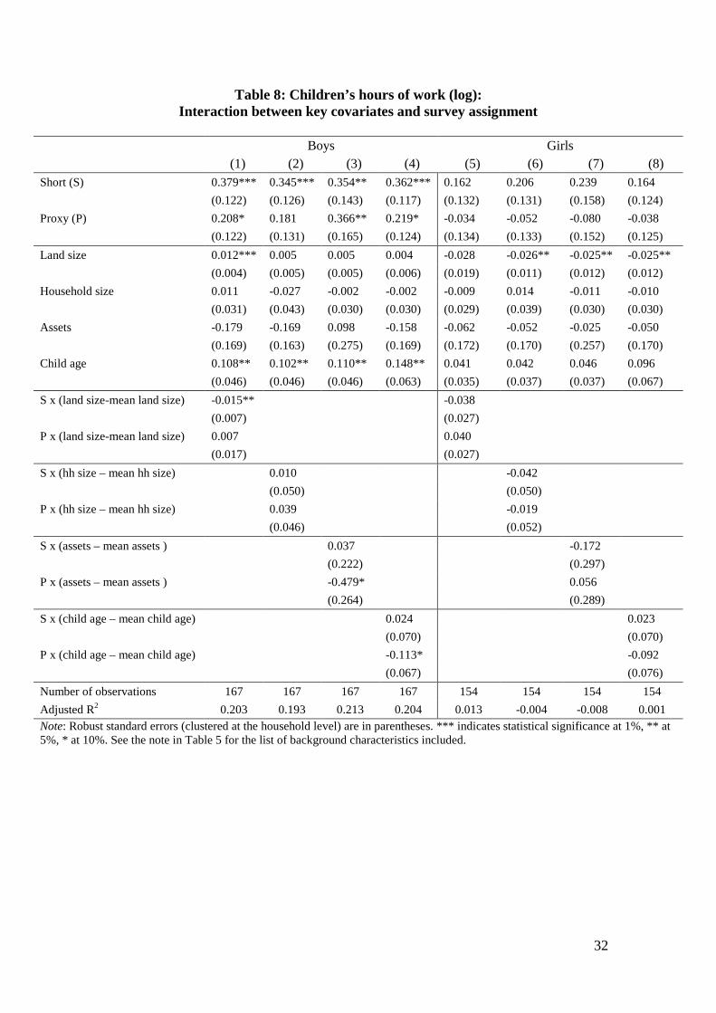
We find fewer statistically significant effects of survey design choices in estimates
associated with the four covariates we focused on when we consider the effects of
those covariates on girls’ or boys’ conditional hours (Table 8). For girls, we find no 15 The aim of these results is to explore whether survey methods may affect the estimated coefficients. A more detailed analysis would be needed to give a precise meaning to the results. For instance, we limit ourselves to a simple linear relationship and do not explore the interaction with quadratic covariates, which may or may not be more appropriate in some instances. 16 As before, we only report the results for the short and proxy indicators. Including an additional indicator variable for the short proxy module yields similar results.
19
differential effect associated with proxy or short modules with respect to land
holdings, household size, assets, and the child’s age. For boys, only land holdings are
associated with a differential effect of the short questionnaire. Boys from households
with larger land size have less of a gap between hours reported by the short vs.
detailed modules. Proxy reporting yields greater hours (as in Table 5) but this increase
is attenuated for older boys, and is reversed (i.e., proxy respondents generate fewer
hours than self-respondents) for boys living in households with a higher level of
assets. Although other results are not statistically significant, the small sample size
permits only the statistically significant detection of large effects.
Results in Tables 7 and 8 indicate that different survey methods may generate
employment statistics that are not only different at the mean, but also vary as key
covariates vary. That is, the estimation of the economic relationships of interest to the
researcher can be affected by the survey method. For both girls’ and boys’ LFP, we
find that the size of the effect of the short versus detailed module varies depending on
household assets and the child’s age. Given the central importance in the literature of
the effect of household wealth and household size on girls’ participation in domestic
duties—like childcare and food preparation—and economic activities—like the
processing of food for market sale—our results raise important questions on the
empirical estimation of these effects and point to the need for more research in this
direction.
Cost implications
Alternative survey designs will have cost implications that have to be weighed against
the value of “better” data. The difference in length between the detailed and the short
module we used in our experiment was small; using the detailed module added only a
few minutes to the average duration of the interview, according to field work reports
from enumerators and supervisors. The cost implication of using a detailed rather than
a short module, therefore, is also small. The additional cost of printing slightly longer
questionnaires and the extra data entry requirement are only marginally larger for the
detailed questionnaire.
20
By contrast, using proxy instead of self-reports involves substantial savings. The use
of self-reports increases the length of field work because more days are spent in each
sample village to locate and interview respondents. This survey experiment was
carried out in conjunction with a larger consumption expenditure experiment, which
required survey teams to spend a full two weeks in a village anyway. We cannot
determine the additional field days that would be needed to complete self-report
compared to proxy labor modules. However, based on field experience, we can
roughly calculate that for two days spent in a village using proxy respondents, the
survey team would need at least one more day to track down self-reports. This
corresponds to a 33 percent increase in the length of time spent on actual field work.
We can assume that all variable costs of field staff (per diems, lodging costs), often
the largest category of survey costs, would increase by 33 percent. Transport costs
may also raise if field teams used a team vehicle to track down respondents for self-
reports. Given that the results of our experiment indicate that using self-reports
instead of proxy respondents does not alter significantly the employment statistics
collected, we can conclude—even without a rigorous cost-benefit calculation—that
using self-reports in this case (for this sample and this type of statistics) would not be
worth the extra cost required.
5. Conclusions
Child labor has received increasing attention over the past decade and empirical
measurement has now become common practice. How child labor is measured does
differ across countries and within countries over time, potentially creating problems
of comparability. Little is known about whether different survey methods generate
different results for child labor statistics or whether the fluctuations we observe in
child labor data are explained by other factors. This paper presents a randomized
experiment whereby we use two commonly varied survey designs, the level of detail
in the questionnaire and the choice of respondent, to estimate the effects of these
survey features on the labor statistics they generate.
Our findings suggest that using a short employment module generates a much lower
incidence of child labor, once the percentage of boys and girls who declare their main
occupation was “domestic duties” are correctly classified—as per the ILO definition
21
of employment—as “not in work,” and also has some effect on working hours. Both
boys and girls are reported to have lower participation in agriculture and more in
domestic duties using the short module. Response by proxy seems to have no effect
on employment statistics compared with the self-reported response by the child. These
observations are confirmed when controlling for a wide range of individual,
household, and village characteristics. When we use probit analysis to estimate the
marginal effect of the two survey types, we find that the short module yields 17
percentage points lower participation rates for boys and 23 percentage points lower
for girls. Using a multinomial logit, we find that both boys and girls are less likely to
be reported in agriculture and other sectors than in no work and domestic duties when
using the short module. However, response by proxy produces statistics that are not
significantly different from self-response. This is in sharp contrast with the effect of
survey methods on labor statistics of adults, where response by proxy appears to have
the largest impact (see Bardasi et al., 2010). Our finding that there is no significant
discrepancy in child labor force participation statistics between proxy and self-reports
(that is, between the situation in which questions are asked to adults or the children
themselves) is particularly reassuring.17 When discussing the choice of the
respondent, in particular the use of household surveys to obtain information on child
labor, the ILO guidelines state that “...With regard to respondents, the general practice
is to address survey questions to the most knowledgeable adult member of the
household (or sometimes the head of household, who is often also the parent or
guardian of the working child). However, sections of the questionnaire may be
addressed to the children themselves, particularly on hazards at the work place, and
the main underlying reason for working.” (ILO, 2008, para 49) The ILO document
also states the importance of respecting ethical standards to make sure that children
are not adversely affected by their participation in the survey, when they are
respondents. So, in situations where it is not possible to interview the children directly
or it is considered inappropriate, our results indicate that employment statistics should
not be significantly affected.
17 An alternative view is that children and parents (and other proxy respondents) are equally disinclined to reveal the actual extent of child labor due to social stigma – that it is hidden from surveyors. As discussed in the Introduction, we consider this stigma to be minimal in this setting. This does imply that these results may not be germane in contexts where people would want to hide or deny the extent to which children work.

22
Our results suggest that for measuring child labor, the World Bank and ILO
recommendation of using a detailed, self-reported questionnaire has an effect
primarily through the appropriate screening of children into reporting their labor
market activities. The type of questionnaire has a limited effect on measuring hours
correctly for the whole sample, as our results on unconditional hours worked in Table
3 suggest. The screening questions may have an important role in reducing a source of
misreporting in labor modules, namely, the respondent’s confusion over the economic
distinction between labor market activities and domestic activities.
The lower LFP but longer hours for those in employment estimated with the short
questionnaire compared with the detailed module suggests that more marginal jobs
are being under-reported when using the short employment module. This indicates
that the survey design may matter more for certain groups of individuals than others,
such as in this example for children who combine work with school.
We also find evidence that estimated coefficients reflecting the relationship between
child labor force participation and economic variables that have been found to be
significant explanatory variables, like household size, assets, and land owned by the
household, can differ depending on the survey method used.
These results provide clear evidence that survey design does matter for measuring and
explaining child labor outcomes. Interestingly, the effects are different from those for
adults found in our previous work. In the case of children, what appears to be
important is a questionnaire design that defines more precisely (through screening
questions) what “work” means, while using a proxy or asking the child directly does
not seem to affect employment statistics. For adults we came to the opposite
conclusions (Bardasi et al., 2010).
Although we considered only two dimensions of survey design, our results send a
strong signal. In order to compare, monitor, and analyze child labor, more attention
should be placed in harmonizing the survey approach that generates the data. Rapid
declines or increases in child labor that are solely due to differences in survey
approaches may send wrong signals to policymakers. Although shorter, rapid
appraisal questionnaires might be advantageous from a policy perspective and for cost
23
reasons—and may be a very acceptable method for adults if they self-report
information, based on our research findings—their ability to provide reliable child
labor statistics needs to be further considered. These few additional screening
questions in the detailed questionnaire—to clarify the meaning of the concept of
work—come at very little cost for survey field work.
Our results are also an implicit plea for additional, similar survey experiments, as they
leave important questions unanswered. Whereas the experiments used in this paper
(especially the short vs. detailed questionnaire one) focus on existing survey
instruments, future work may want to explore the effects that newly designed
instruments would have. In particular, combining survey instruments with direct
observation or diary keeping could be especially useful to find out what approach
works best, and to help define a “gold standard,” on which there is currently no
agreement. Another fruitful way forward would be to implement survey experiments
to investigate issues related to the System of National Accounts categorization. The
experiment used in this paper, while not well suited to address these issues, indicates
that how respondents classify children’s work may not always be clear. Finally, a
more precise way to identify a “pure” proxy effect would involve comparing data on
the same person from proxy and self-response. Although this type of experiment
could not be implemented in the setting available to us, this is certainly something
worth considering for future work under different conditions.
24
References
Anker, R. (1983) “Female Labour Force Participation in Developing Countries: A
Critique of Current Definitions and Data Collection Methods.” International Labour Review 122(6): 709-724.
Bardasi, E., K. Beegle, A. Dillon, and P. Serneels (2010) “Do Labor Statistics Depend
on How and to Whom the Questions are Asked? Results from a Survey Experiment in Tanzania.” World Bank Policy Research Working Paper 5192.
Bass, L. (2004) Child Labor in Sub-Saharan Africa. Lynne Rienner Publishers,
Boulder, London. Basu, K., and P.H. Van (1998) “The Economics of Child Labor.” American Economic
Review 88(3): 412–427. Bhalotra, S., and C. Heady (2003) “Child Farm Labor: The Wealth Paradox.” The
World Bank Economic Review 17(2): 197-227. Borgers, N., E. de Leeuw, and J. Hox (2000) “Children as Respondents in Survey
Research: Cognitive Development and Response Quality.” Bulletin de Méthodologie Sociologique 66: 60-75.
Dillon, A. (2010) “Measuring Child Labor: Comparisons between Hours Data and a
Subjective Module.” Research in Labor Economics 31: 135-159. Edmonds, E. (2005) “Does Child Labor Decline with Improving Economic Status?”
Journal of Human Resources 40(1): 77-99. Edmonds, E.V. (2009) “Child Labor” in T.P Schultz and J. Strauss, Handbook of
Development Economics Volume 4, Elsevier Science, Amsterdam, North Holland, forthcoming.
Guarcello, L., I. Kovrova, S. Lyon, M. Manacorda, and F.C. Rosati (2009) “Towards
Consistency in Child Labour Measurement: Assessing the Comparability of Estimates Generated by Different Survey Instruments.” Understanding Children's Work Project Draft Working Paper.
ILO (2004) Child Labour Statistics: Manual on methodologies for data collection through surveys. Geneva.
ILO (2008) Child Labour Statistics: Report III. Geneva.
Schaffner, J. (2000) “Chapter 9 Employment,” in P. Glewwe and M. Grosh (eds.), Designing Household Survey Questionnaires for Developing Countries: Lessons from 15 Years of the Living Standards Development Study. Oxford University Press (for the World Bank).

25
Table 1: Household characteristics by survey assignment
Households by survey assignment F-test of equality of coefficients
across groups
Detailed Detailed Short Short
self-report proxy self-report proxy
Head: female (%) 20.4 22.3 26.7 19.3 0.544
Head: age 48.4 47.3 48.7 48.4 0.882
Head: years of schooling 4.2 4.5 4.6 4.7 0.778
Head: married (%) 74.3 76.2 71.6 81.5 0.277
Household size 6.8 6.0 6.2 6.6 0.046
Adult equivalence household size 5.5 4.9 5.1 5.3 0.082
Share of members less 6 years 16.7 15.5 15.4 16.3 0.876
Share of members 6-15 years 41.2 41.9 42.1 41.0 0.915
Concrete/tile flooring (non-earth) (%) 16.8 17.7 23.3 23.0 0.451
Main source for lighting is electricity/generator/solar panels (%) 5.3 4.6 10.3 9.6 0.199
Owns a mobile telephone (%) 25.7 24.6 25.0 29.1 0.845
Bicycle (%) 52.2 43.1 45.7 50.4 0.457
Asset index (ln) -0.2 -0.2 -0.1 -0.0 0.206
Owns any land (%) 84.1 87.7 80.2 85.2 0.457
Land size (acres, incld 0s) 4.3 3.2 3.3 4.1 0.082
Month of interview (1=Jan, 12=Dec) 6.4 6.3 6.1 5.9 0.711
Number of households 113 130 116 135 Note: The F-test tests the equality of coefficients across the groups by regressing the group indicators on the household characteristics with clustered household standard errors.
26
Table 2: Children’s household and individual characteristics by survey assignment
Individual survey assignment F-test of equality of coefficients across groups
Detailed Detailed Short Short
self-report proxy self-report proxy
Female (%) 50.0 56.1 45.5 57.6 0.249
Age 12.3 12.4 12.6 12.4 0.706
Years of schooling 3.1 3.0 3.1 3.0 0.972
Head: female (%) 21.6 22.9 27.6 19.4 0.467
Head: age 48.3 47.7 48.7 48.2 0.937
Head: years of schooling 4.3 4.4 4.8 4.6 0.700
Head: married (%) 74.1 75.2 69.9 81.8 0.128
Household size 6.8 6.2 6.3 6.7 0.079
Adult equivalence hh size 5.4 5.0 5.2 5.3 0.135
Share of members less 6 years 16.8 15.5 14.8 16.5 0.811
Share of members 6-15 years 41.2 43.5 43.4 42.8 0.701
Concrete/tile flooring (%) 17.2 17.2 23.6 21.8 0.555
Main source for lighting is electricity/generator/solar panels (%) 6.0 4.5 9.8 8.8 0.348
Owns a mobile telephone (%) 25.0 23.6 26.0 28.4 0.769
Bicycle (%) 52.6 42.7 47.2 50.0 0.533
Asset index (ln) -0.2 -0.2 -0.1 -0.0 0.264
Owns any land (%) 82.8 88.5 80.5 85.3 0.271
Land size (acres, incld 0s) 4.2 3.3 3.4 4.2 0.184
Month of interview (1=Jan, 12=Dec) 6.4 6.4 6.1 6.0 0.841
Any hours collecting firewood last 24 hours (%) 26.7 31.2 31.7 25.9 0.377
Hours collecting firewood last 24 hours (including 0s) 0.3 0.5 0.4 0.4 0.922
Any hours collecting water last 24 hours (%) 60.3 60.5 70.7 66.5 0.615
Hours collecting water last 24 hours (including 0s) 0.5 0.5 0.5 0.5 0.306 Number of individuals 116 157 123 170 Note: The F-test tests the equality of coefficients across the groups by regressing the group indicators on the household characteristics with clustered household standard errors. Among the sample assigned to self-report, 3 children were unavailable and are re-categorized as a proxy response for the detailed module.
27
Table 3: Child labor statistics of the main job by survey assignment
A. B. Short Detailed Diff Proxy Self-rep Diff
Labor force participation (%)
Boys 55.4 70.9 -15.4*** 61.7 64.0 -2.3
(0.50) (0.46) (0.06) (0.49) (0.48) (0.06)
Girls 44.2 58.9 -14.7*** 50.0 53.5 -3.5
(0.50) (0.49) (0.06) (0.50) (0.50) (0.06)
Weekly hours last week (unconditional)
Boys 12.0 11.2 0.8 11.5 11.7 -0.2
(15.5) (12.4) (1.7) (13.2) (15.0) (1.7)
Girls 9.0 9.7 -0.7 9.0 9.9 -0.9
(13.7) (11.6) (1.5) (12.7) (12.7) (1.5)
Weekly hours last week (conditional on LFP=1)
Boys 21.7 15.7 6.0*** 18.7 18.3 0.3
(14.9) (12.0) (2.1) (12.3) (15.1) (2.1)
Girls 20.3 16.5 3.8** 18.0 18.5 0.5
(13.9) (10.8) (2.0) (12.8) (11.8) (2.0)
Hours of firewood collection in last 24 hours
Boys 0.4 0.5 -0.1 0.6 0.3 0.3**
(0.9) (0.9) (0.1) (1.0) (0.7) (0.1)
Girls 0.3 0.3 0.0 0.3 0.4 -0.1
(0.6) (0.7) (0.1) (0.6) (0.7) (0.1)
Hours of water collection in last 24 hours
Boys 0.4 0.4 0.0 0.4 0.4 0.0
(0.7) (0.7) (0.1) (0.5) (0.8) (0.1)
Girls 0.6 0.6 0.0 0.6 0.6 0.0
(0.7) (0.7) (0.1) (0.8) (0.6) (0.1)
Note: Standard deviation of variables and the standard error of the differences are in parentheses.
28
Table 4: Child’s main activity in their main job by survey assignment
Boys Girls
A. Short or detailed Short Detailed Diff
Short Detailed Diff
Agriculture 52.5 68.5 -16.0*** 42.9 58.2 -15.4***
Other sectors 2.9 2.4 0.5 1.3 0.7 0.6
Domestic Duties 30.2 9.4 20.8*** 43.5 8.2 35.3***
No work 14.4 19.7 -5.3 12.3 32.9 -20.6***
Number of individuals 139 127 154 146
B. Proxy or self-rep Proxy Self-rep Diff
Proxy Self-rep Diff
Agriculture 60.3 60.0 0.3 49.5 51.8 -2.3
Other sectors 1.4 4 -2.6* 0.5 1.8 -1.3
Domestic Duties 21.3 19.2 2.1 23.7 20.2 3.5
No work 17.0 16.8 0.2 23.1 20.2 2.9
Number of individuals 141 125 186 114 Note: Other sectors are specifically listed on the questionnaire and include mining/quarrying, manufacturing/processing, gas/water/electricity, construction, transport, trading, personal services, education/health, public administration, and other. *** indicates statistically significant mean differences with the detailed self-report at 1%, ** at 5%, * at 10%.
29
Table 5: Regression analysis of labor statistics by survey assignment
Labor force participation in main job
over the last 7 days Conditional hours worked in main job
over the last 7 days
Pooled Boys Girls Pooled Boys Girls
Short -0.165*** -0.194*** -0.157** 0.251*** 0.366*** 0.183
(0.047) (0.065) (0.064) (0.087) (0.117) (0.127)
Proxy -0.072 -0.039 -0.058 0.052 0.206* -0.059
(0.047) (0.066) (0.066) (0.090) (0.123) (0.130)
Observations 566 266 300 321 167 154
Note: Robust standard errors (clustered at the household level) are in parentheses. *** indicates statistical significance at 1%, ** at 5%, * at 10%. Regressions include controls for household size, female headship, share of members under 6 years, share of members 6-15 years, share of members over 60, asset index, acres of land owned, child’s age, whether child ever attended school, and district dummy variables. LFP estimates are conducted using a probit model and we report marginal effects.
30
Table 6a: Regression analysis of main activity by survey assignment
Pooled Boys Girls
Agriculture + other sectors
Domestic work
Agriculture + other sectors
Domestic work
Agriculture + other sectors
Domestic work
Short -0.176*** 0.330*** -0.161** 0.216*** -0.168** 0.423***
(0.048) (0.038) (0.065) (0.046) (0.071) (0.055)
Proxy -0.065 0.017 -0.040 0.019 -0.050 -0.012
(0.048) (0.038) (0.061) (0.040) (0.071) (0.062)
Observations 566 566 266 266 300 300
Note: The multinomial logit model uses three categories: agriculture and other sectors, domestic work, and the omitted category, no work. Marginal effects are reported. See the note in Table 5 for the list of background characteristics included. See the note in Table 4 for an explanation of other sectors. Robust standard errors (clustered at the household level) are in parentheses. *** indicates statistical significance at 1%, ** at 5%, * at 10%.
Table 6b: Predicted distribution from MNL estimates
Actual Predicted distribution from MNL regression
Short Detailed Proxy Self-report
All
Ag or other sectors 56.7 49.9 63.2 54.6 59.6
Domestic work 23.5 37.9 8.2 24.0 23.4
No work 19.8 12.2 28.5 21.4 17.3
Boys
Ag or other sectors 62.8 54.3 68.1 60.1 63.3
Domestic work 20.3 31.5 8.4 21.0 19.3
No work 16.9 14.2 23.5 19.0 17.4
Girls
Ag or other sectors 51.3 45.4 58.1 50.1 53.9
Domestic work 26.3 44.3 8.3 26.6 27.8
No work 22.3 10.4 33.5 23.3 18.2
31
Table 7: Children’s labor force participation: Interactions of key covariates and survey assignment
Boys Girls (1) (2) (3) (4) (5) (6) (7) (8)
Short (S) -0.205*** -0.211*** -0.226*** -0.208*** -0.154** -0.153** -0.182*** -0.159**
(0.067) (0.067) (0.069) (0.066) (0.064) (0.065) (0.063) (0.065)
Proxy (P) -0.040 -0.028 -0.011 -0.044 -0.085 -0.068 -0.054 -0.050
(0.068) (0.068) (0.070) (0.067) (0.070) (0.067) (0.067) (0.066)
Land size 0.022 0.006 0.005 0.007 0.016 0.003 0.001 0.000
(0.014) (0.007) (0.008) (0.008) (0.012) (0.005) (0.006) (0.006)
Household size 0.051*** 0.050 0.051*** 0.053*** 0.009 0.005 0.010 0.008
(0.019) (0.030) (0.019) (0.019) (0.015) (0.023) (0.015) (0.015)
Asset index 0.204*** 0.207*** 0.183** 0.206*** 0.115* 0.122** 0.032 0.125**
(0.060) (0.059) (0.084) (0.060) (0.059) (0.059) (0.111) (0.058)
Child age 0.057** 0.060*** 0.064*** 0.121*** 0.050** 0.049** 0.049** 0.020
(0.022) (0.023) (0.023) (0.041) (0.024) (0.024) (0.023) (0.041)
S x (land size-mean land size) -0.019 0.018**
(0.015) (0.009)
P x (land size-mean land size) -0.011 -0.021
(0.015) (0.013)
S x (hh size – mean hh size) -0.030 0.045*
(0.034) (0.026)
P x (hh size – mean hh size) 0.029 -0.029
(0.034) (0.025)
S x (assets – mean assets ) 0.215** 0.170**
(0.091) (0.086)
P x (assets – mean assets ) -0.105 0.010
(0.087) (0.098)
S x (child age – mean child age) -0.077* 0.067*
(0.041) (0.039)
P x (child age – mean child age) -0.039 -0.015
(0.040) (0.040)
Number of observations 266 266 266 266 300 300 300 300
Adjusted R2 0.287 0.285 0.297 0.292 0.237 0.230 0.230 0.230 Note: Robust standard errors (clustered at the household level) are in parentheses. *** indicates statistical significance at 1%, ** at 5%, * at 10%. See the note in Table 5 for the list of background characteristics included.
32
Table 8: Children’s hours of work (log): Interaction between key covariates and survey assignment
Boys Girls (1) (2) (3) (4) (5) (6) (7) (8)
Short (S) 0.379*** 0.345*** 0.354** 0.362*** 0.162 0.206 0.239 0.164
(0.122) (0.126) (0.143) (0.117) (0.132) (0.131) (0.158) (0.124)
Proxy (P) 0.208* 0.181 0.366** 0.219* -0.034 -0.052 -0.080 -0.038
(0.122) (0.131) (0.165) (0.124) (0.134) (0.133) (0.152) (0.125)
Land size 0.012*** 0.005 0.005 0.004 -0.028 -0.026** -0.025** -0.025**
(0.004) (0.005) (0.005) (0.006) (0.019) (0.011) (0.012) (0.012)
Household size 0.011 -0.027 -0.002 -0.002 -0.009 0.014 -0.011 -0.010
(0.031) (0.043) (0.030) (0.030) (0.029) (0.039) (0.030) (0.030)
Assets -0.179 -0.169 0.098 -0.158 -0.062 -0.052 -0.025 -0.050
(0.169) (0.163) (0.275) (0.169) (0.172) (0.170) (0.257) (0.170)
Child age 0.108** 0.102** 0.110** 0.148** 0.041 0.042 0.046 0.096
(0.046) (0.046) (0.046) (0.063) (0.035) (0.037) (0.037) (0.067)
S x (land size-mean land size) -0.015** -0.038
(0.007) (0.027)
P x (land size-mean land size) 0.007 0.040
(0.017) (0.027)
S x (hh size – mean hh size) 0.010 -0.042
(0.050) (0.050)
P x (hh size – mean hh size) 0.039 -0.019
(0.046) (0.052)
S x (assets – mean assets ) 0.037 -0.172
(0.222) (0.297)
P x (assets – mean assets ) -0.479* 0.056
(0.264) (0.289)
S x (child age – mean child age) 0.024 0.023
(0.070) (0.070)
P x (child age – mean child age) -0.113* -0.092
(0.067) (0.076)
Number of observations 167 167 167 167 154 154 154 154
Adjusted R2 0.203 0.193 0.213 0.204 0.013 -0.004 -0.008 0.001 Note: Robust standard errors (clustered at the household level) are in parentheses. *** indicates statistical significance at 1%, ** at 5%, * at 10%. See the note in Table 5 for the list of background characteristics included.

33
Annex
Table A1 - Key employment questions in the short and detailed questionnaires Short questionnaire Detailed questionnaire 1. During the past 7 days, has [NAME] worked for
someone who is not a member of your household, for example, an enterprise, company, the government or any other individual? YES...1 (»3) NO.....2 (question repeated for the past 12 months)
3. During the past 7 days, has [NAME] worked on a farm owned, borrowed or rented by a member of your household, whether in cultivating crops or in other farm maintenance tasks, or have you cared for livestock belonging to a member of your household? YES...1 (»5) NO.....2 (question repeated for the past 12 months)
5. During the past 7 days, has [NAME] worked on his/her own account or in a business enterprise belonging to he/she or someone in your household, for example, as a trader, shop-keeper, barber, dressmaker, carpenter or taxi driver? YES...1 (»7) NO.....2 (question repeated for the past 12 months)
1. Did [NAME] do any type of work in the last seven days? Even if for 1 hour. YES...1 (»3) NO.....2 (question repeated for the past 12 months)
7. CHECK THE ANSWERS TO QUESTIONS 1, 3 AND 7. (WORKED IN LAST 7 DAYS) ANY YES..1 ALL NO.....2 (»37)
3. What is [NAME]'s primary occupation in [NAME]'s main job? (MAIN OCCUPATION IN THE LAST 7 DAYS) a. OCCUPATION b. OCCUPATION CODE
8. What is [NAME]'s primary occupation in [NAME]'s main job? (MAIN OCCUPATION IN THE LAST 7 DAYS) a. OCCUPATION b. OCCUPATION CODE
4. In what sector is this main activity? AGRICULTURE. . . . . . . . . . . . . . 1 MINING/QUARRYING . . . . . . . . . . . 2 MANUFACTURING/ PROCESSING. . . . . . . 3 GAS/WATER/ELECTRICITY. . . . . . . . . 4 CONSTRUCTION . . . . . . . . . . . . . 5 TRANSPORT. . . . . . . . . . . . . . . 6 BUYING AND SELLING . . . . . . . . . . 7 PERSONAL SERVICES. . . . . . . . . . . 8 EDUCATION/HEALTH . . . . . . . . . . . 9 PUBLIC ADMINISTRATION. . . . . . . . .10 DOMESTIC DUTIES. . . . . . . . . . . .11 OTHER, SPECIFY . . . . . . . . . . . .12
9. In what sector is this main activity? AGRICULTURE. . . . . . . . . . . . . . 1 MINING/QUARRYING . . . . . . . . . . . 2 MANUFACTURING/ PROCESSING. . . . . . . 3 GAS/WATER/ELECTRICITY. . . . . . . . . 4 CONSTRUCTION . . . . . . . . . . . . . 5 TRANSPORT. . . . . . . . . . . . . . . 6 BUYING AND SELLING . . . . . . . . . . 7 PERSONAL SERVICES. . . . . . . . . . . 8 EDUCATION/HEALTH . . . . . . . . . . . 9 PUBLIC ADMINISTRATION. . . . . . . . .10 DOMESTIC DUTIES. . . . . . . . . . . .11 OTHER, SPECIFY . . . . . . . . . . . .12

34
Table A2. Self-report and proxy selection process
Self-report Proxy Eligibility rule: Eligibility rule for selecting proxy respondent: Individuals age 10+ Individuals age 16+ Eligibility rule for selecting subjects for proxy reporting: Individuals age 10+ Selection: Selection: Random selection of 2 respondents among eligible respondents
1. Random selection of 1 proxy respondent among eligible proxy respondents. The proxy respondent self-reports for him/herself
2. Random selection of 2 subjects for proxy reporting (excluding the proxy respondent selected)