explaining crime growth in russia during transition: economic and
TRANSCRIPT
1
Yury Andrienko†
Explaining Crime Growth in Russia during Transition: Economic and
Criminometric Approach*
February, 2001
Abstract.
This paper presents a simple model of a rational offender based on cost-benefit analysis with uncertain income and costs. In the empirical part we estimate a system of dynamic crime supply equation and its first difference by using Generalized Method of Moments with moment conditions generated by assumption of endogeneity of explanatory variables. We use a set of socio-economic, demographic and other indicators as explanatory variables, including proxies for criminal experience, alcohol and drug consumption, and the strength of Police. Data used are panel data from 1990 to 1998 for 70 Russian regions. In the study crime is represented by homicide and larceny as proxies for violent and property crimes respectively. Both types of crime are found to be persistent over time. There is a strong deterrent effect arising from Police activity but this effect is very restricted indicating that enforcement activity is important but could not prevent further crime growth. High level of education prevents people from committing either types of crime. Dramatically increasing drug consumption led to a rise in either type of criminal activity. Higher alcohol consumption is found to be responsible for growth in violence during transition. Moreover, in spite of common belief on the West, the largest part of homicides is not associated with criminal gangs but a result of outbreak of aggression within family and neighborhood generally caused by alcohol intoxication. Family disruption in 90-es is also highly responsible for crime growth. Other socio-economic indicators have an opposite impact on violent and property crimes. We find that with higher income inequality, and lower real income and unemployment rate property crimes are substituted by violence. We can expect therefore further total crime growth once Russia has sustainable economic growth, with less violence but with more property and economic crimes. At the same time total crime rate in Russia is still below the level in other European countries, even if we take into account higher unreported rate in Russia.
* The author would like to thank Rudiger Ahrend and other CEFIR, former RECEP, members for the idea of the project initialization, EERC experts and conference participants for helpful comments and concernment in the project results. Also I am indebted to Ministry of Interior officials, Eugenia Koshkina from Institute of Narcology, and Alexander Nemtsov from Institute of Psychology for data providing. All remaining errors are the responsibility of the author. Financial support of the Eurasia foundation is gratefully acknowledged.
† Economist at Centre for Economic and Financial Research (CEFIR), Moscow.
2
Contents.
INTRODUCTION. 3
I. HISTORIC DEVELOPMENT OF CRIME IN RUSSIA. 4
II. LITERATURE REVIEW. 9
III. MODELS AND METHODOLOGY. 12
III.i. Theoretical and econometric models. 12
III.ii. Methodology. 15
IV. EMPIRICAL PART. 18
IV.i. Data. 19
IV.ii. Regression results. 21
V. POLICY IMPLICATIONS. 26
REFERENCES. 28
APPENDIX. 31
3
Introduction.
It is quite clear that epochal changes in economic, social, political environment in
Russia could be resulted in changes of people incentives to criminal activity. The state
lost its control over the people minds and they accommodated fast to new conditions of
freedom. Changes in moral norms have made Russians more patient to previously
unacceptable activities. As a result society was engulfed in a criminal deluge. No need to
say that high stress from reforms and worsened economic conditions was aggravated by
felling of unsafety when people are in fear of their lives.
The purpose of this project is to shed some light on possible factors of crime
growth in Russia during transition. Among the causes of crime growth mentioned in a
public opinion poll held in 1991, the main answers were (i) a fall in the standards of living
(mentioned by 73 % of respondents), (ii) passivity and indecision of the authorities (56
%), (iii) failure to punish the offenders (50 %).
It is commonly accepted that democratization of society and transition to market is
inevitably accompanied by such an evil as the high total crime rate (e.g. emergence of
private property leads to lucrative crime against it). However, some other negative
consequences from openness in Russian society are on the surface, like increased
intentional and planned homicides, economic crimes and drug spreading. The last two
types of crime have shown the most drastic increase and are responsible for the dramatic
growth in total crime rate in Russia during the 90-es.
Now, Russia has an entire range of social problems previously associated only
with capitalist society, i.e. poverty, unemployment, inequality, homelessness, drug
addiction, along with other peculiarities, such as wage arrears, nonpayment, barter, high
corruption, etc. All of them could be the causes and partially the consequences of crime
growth in Russia.
This study is the first empirical paper on factors of crime in Russia. We want to
check whether drastic changes in social and economic indicators, such as income decline,
rise in inequality and unemployment had an impact on people incentives to illegal
behavior. The deterioration of these indicators should have resulted in higher
attractiveness of involvement in the illegal sector, even if it is becoming more risky.
Probably, the influence of those indicators was different for major types of crime. Thus,
we are going to consider two types of crime, homicide and larceny-thefts, as
representatives of violent and property crimes. The second hypothesis we are going to test

4
is that the efficiency of the law enforcement agencies also impact on the crime rate. Is
there sufficient control of the state over the crime situation? Does the probability to be
detected deter a criminal? Another question that may be raised in this project is whether
economic and social instruments rather than law enforcement can prevent people from
crime. As is recognized in other countries, for example, greater employment
opportunities, training at school or institutions of higher learning keep youth from illegal
activities.
Looking at crime distribution across the Russian regions, one can notice that there
are stable differences among the regions. Crime increases from west to east and the
pattern (not levels) is rather stable in time dimension. This can mean criminal inertia or
crime persistency over time, the next hypothesis to be tested.
The main question we want to answer is “What are the main determinants of
criminal behavior in Russia and what policies, law-enforcement-related and socio-
economic, can be used to control or combat crime?” We will try to concentrate more on
basic crime determinants (so called factors of crime) known from the empirical literature.
Data we are going to use in the project are panel data that is pooled time-series
from 1990 to 1998 and cross-section data for 89 subjects of Russian Federation. Crime
supply equation in dynamic form complemented with its first differenced form will be
estimated as a system by General Method of Moments. Explanatory variables in the
model are allowed to be endogenous. Instruments to be used are from moment conditions
implied by assumption of endogeneity.
The paper consists of five main parts. The First section describes the historic
development of crime in USSR and Russia, and changes occurred during transition
period. The Second part contains literature review. In the Third section we present
theoretical and empirical models, including methodological issues. Data and results are
given in the Forth section. And the last section concludes.
I. Historic development of crime in Russia.
Crime was a problem in Russia even at the beginning of XX century. In the tsarist
Russia the number of criminal cases was very big, on the level of 2.5 million, i.e.
approximately the same rate as in the last decade of the XX century. The October
revolution led to a dramatic economic decline and simultaneously to growth in crime.
Then, as we know, under the Soviet regime the state was able to cope both with crime and

5
political freedom by means of cruel repression. Criminal statistics collection was
established in USSR in 1922 and it reported astounding 2.9 % of population convicted in
1924, coming down to 1.7 and 1.8 in 1925 and 1926. It is noteworthy, that it is much
higher than conviction rate 0.7 % of population in 1999. After Stalin’s death and further
political warming in the 50-s, the crime rate in USSR began to rise gradually following a
worldwide trend in crime. We recognize that the largest part of crimes during Stalin’s
time could be not civil but rather political crimes. Downward trend on the figure below
reflects, to my mind, the ability of the - in essence - police state, to keep citizens under
control and to suppress freethinking with savagery. On the other hand, as Soviet Union
had the boggled imagination economic growth at that time, which is usually accompanied
by the rise in crime activity in a democratic society, the deterrent effect from police and
repression was obviously much higher than we may think.
Numbe r of crime s pe r 100'000 population in USSR, 1920-1990
0
500
1000
1500
2000
1920 1930 1940 1950 1960 1970 1980 1990
Source: normalized figure from Kudryavtsev V. N., "Sovremennie prob lemi b orb i s pres tupnostyu v Ross i i", Ves tnik Ross iyskoy Akademii Nauk, vol 69, # 9, p. 790-797.
After the beginning of the democratization process in the Soviet Union or in
Gorbachev’s epoch in 1985 the hopes of the Russians for the end of the command
economy were very high and looked realistic. The euphoria of acquired freedom in fact
resulted in some improvements in the economic and the crime situation, but since 1988
irreversible processes of further democratization in political and economic life continued,
which led to an incredible growth in crime rate. One of the much merit of Gorbachev’s
politics was opening of criminal statistics to public, which was closed for more than 50
years of the Communist regime. To our mind inability of law enforcement system to cope
with increased crime was the main cause of crime wave that began at the end of 80-s. The
Soviet penal system, the most severe in the world, that kept in custody about 2 million
6
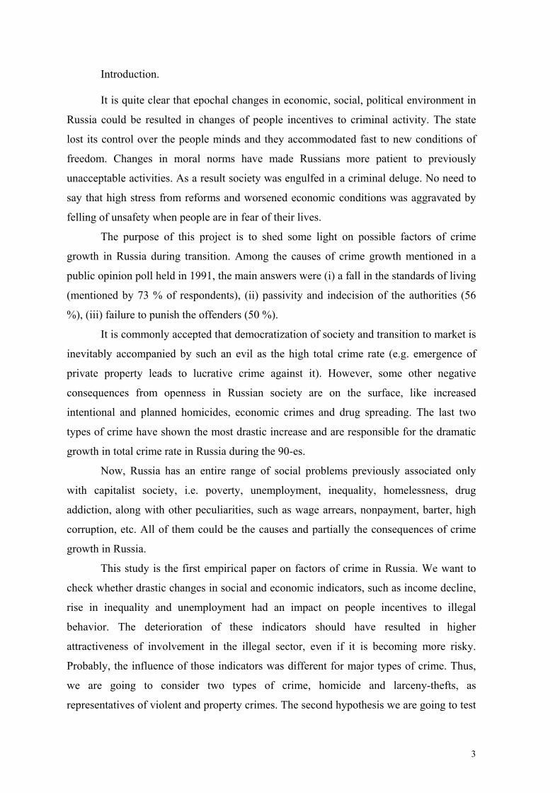
people (0.7 % of population) in the mid of the 80-s1, together with police force were
unable to fulfill their duties after the democratic revolution in the
society.
Crime rate in Russia, 1985-1999.
0
500
1000
1500
2000
2500
3000
3500
1985
1986
1987
1988
1989
1990
1991
1992
1993
1994
1995
1996
1997
1998
1999
0
5
10
15
20
25
30
35
Total number of registeredcrimes, thousands (left scale)
Homicides and attempedhomicides, thousands (rightscale)
Source: Goscomstat (1999).
By the time the economic liberalization was initiated by Gaidar’s cabinet at the
beginning of 1992, the crime rate was already 80 % higher than in 1988 and had grown by
further 30 % before it stabilized in 1993 (see figure above). The period of relative
improvement in 1994-1997 in Russia was followed by a rise in crime after the 1998 crisis.
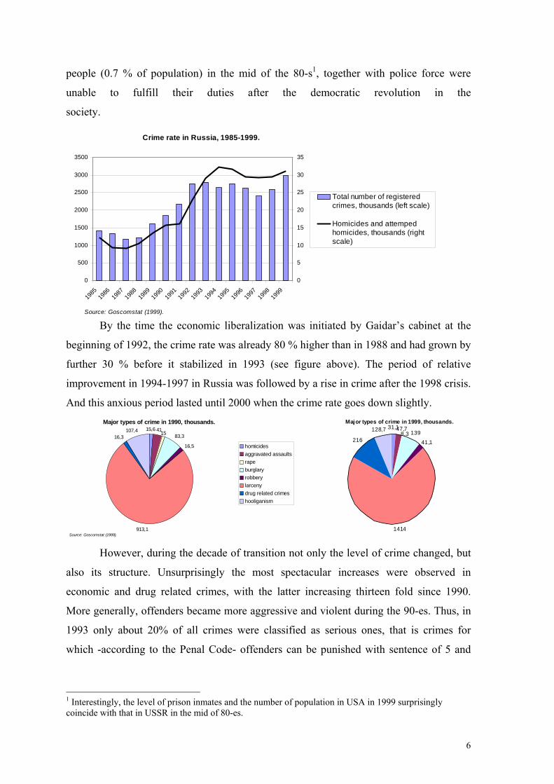
And this anxious period lasted until 2000 when the crime rate goes down slightly. Major types of crime in 1990, thousands.
83,3
913,1
16,3107,4 15,6
1541
16,5 homicidesaggravated assaultsrapeburglaryrobberylarcenydrug related crimeshooliganism
Source: Goscomstat (1999).
However, during the decade of transition not only the level of crime changed, but
also its structure. Unsurprisingly the most spectacular increases were observed in
economic and drug related crimes, with the latter increasing thirteen fold since 1990.
More generally, offenders became more aggressive and violent during the 90-es. Thus, in
1993 only about 20% of all crimes were classified as serious ones, that is crimes for
which -according to the Penal Code- offenders can be punished with sentence of 5 and
1 Interestingly, the level of prison inmates and the number of population in USA in 1999 surprisingly coincide with that in USSR in the mid of 80-es.
Major types of crime in 1999, thousands.
1414
216
128,7
41,1
13947,731,1
8,3
7
more years of imprisonment. Alarmingly the percentage of serious crimes had jumped to
60 per cent in 1998.
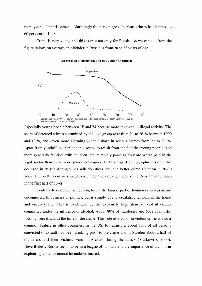
Crime is very young and this is true not only for Russia. As we can see from the
figure below, on average an offender in Russia is from 20 to 33 years of age.
0 10 20 30 40 50 60 70 80
Population
Criminals
Age profiles of criminals and population in Russia
Source: Kudryavtsev V. N., "Sovremennie problemi borbi s prestupnost'u v Rossii", Vestnik Rossiyskoyakademii nauk, vol 69, # 9, p. 790-797.
Especially young people between 18 and 24 became more involved in illegal activity. The
share of detected crimes committed by this age group rose from 21 to 26 % between 1990
and 1998, and -even more alarmingly- their share in serious crimes from 22 to 29 %.
Apart from youthful exuberance this seems to result from the fact that young people (and
more generally families with children) are relatively poor, as they are worse paid in the
legal sector than their more senior colleagues. In this regard demographic disaster that
occurred in Russia during 90-es will doubtless result in better crime situation in 20-30
years. But pretty soon we should expect negative consequences of the Russian baby boom
in the first half of 80-es.
Contrary to common perception, by far the largest part of homicides in Russia are
unconnected to business or politics, but is simply due to escalating tensions in the home
and ordinary life. This is evidenced by the extremely high share of violent crimes
committed under the influence of alcohol. About 80% of murderers and 60% of murder
victims were drunk at the time of the crime. This role of alcohol in violent crime is also a
common feature in other countries. In the US, for example, about 60% of all persons
convicted of assault had been drinking prior to the crime and in Sweden about a half of
murderers and their victims were intoxicated during the attack (Markowitz, 2000).
Nevertheless, Russia seems to be in a league of its own, and the importance of alcohol in
explaining violence cannot be underestimated.
8
In spite of this negative development in crime activity during transition period,
Russia still has the crime rate below the level in many Western European countries even
if we take into account the higher rate of not registered crimes in Russia. On the other
hand, the homicide rate in Russia is four-five times higher than in other European
countries and approximately at the same level as the homicide rate in USA and Brazil. It
should be noticed that the high homicide rate in Russia corresponds to other high
mortality rates, like the suicide rate, which is four times as much as in Europe, and even
the general mortality rate. The latter was equal to the European average mortality rate in
1990, about 10 deaths per 1000 population but after five years it was already 50 % higher
than the European average and achieved the level of 14 deaths per 1000 population. It is
also interesting that suicides, homicides and health problems are particularly prevalent in
rural areas. This, together with the fact that most violent crimes occur in the home or
immediate neighborhood, suggests to us that a large part of crimes in Russia is a direct
consequence of hardships associated with a decade of economic decline and epochal
changes. This in turn suggests that the problem is temporary, but positive changes will
probably be slow.
Writing about crime we should not forget about law enforcement activity of the
state. First, we understand that during recession the state was not able to provide adequate
financing for its Criminal Justice and Police System. Thus, efficiency of Police activity,
say measured by the detection rate, diminished sharply2. On the other hand, poor
financing of courts and prisons led to more heavy punishment during transition.
Russia and USA are still on the top of the prison population rating, keeping in the
custody about 0.7 per cent of population. About 1 million people are behind bars in the
prisons and pre-trial detention facilities in Russia. About 20 % of them were convicted in
personal crimes (homicide, rape or assault) and about 25 % committed serious property
crimes (burglary and robbery). In the words of Pristavkin, the head of presidential
commission on pardon, up to 90 % of incarcerated in Russia are not professional
criminals as they had committed a domestic crime.
Prisons and pretrial detention facilities are overcrowded in Russia, often the
density in the latter is lower than one square meter per man, and detainees have to sleep in
three shifts. Convicted people held in correctional institutions are short of food, medicine
and clothes. As a consequence, the risk to become ill with tuberculosis in prison is 58
2 But not in official reports.

9
times higher than the Russian average, and the general mortality rate is 28 times higher.
This is apparently not only due to a lack of resources, but to some degree a conscious
policy of the Russian penal system. Ministry of Interior officials say that they prefer to
keep young men in pretrial detention facilities for as long as possible even for small
delinquencies to show them the whole unattractiveness of being in such a place3. An
unprecedented amnesty in the summer 2000, when about 100,000 people should have
been released from prisons4, did little to improve the situation of those remaining in
custody.
Penal system in Russia, which was inherited from the command regime and
continues to be one of the most severe in the world, needs to be reformed in the direction
of providing population with further democratic freedoms.
II. Literature review.
As Latov writes in his review (Latov, 2000), American economists retain
intellectual prevalence in economic-criminological studies. Western European studies
play the secondary role. Say, Entorf (Entorf, 1997) express regret for absence of modern
research in Economics of crime in Germany. There are few empirical studies of crime in
Russia, if any. Unfortunately, Russian economists and other scientists have not played
their role in studying this vital problem yet. In the words of Latov this paper will be the
first empirical study in Economics of crime in Russia.
Economic models of crime with expected utility maximization approach have been
developed since Becker’s seminal paper (Becker, 1968), in which he proposed a simple
cost-benefit analysis incorporating monetary gains and losses and uncertainty about the
punishment for an illegal activity. The main result of the model is that the probability of
punishment and monetized size of punishment deter an offender that is with their increase
the expected utility reduces. Moreover, an offender with decreasing absolute risk aversion
is more deterred by 1 % increase in the probability in punishment rather than the same rise
in the size of punishment. Also, Becker considers a supply of offence function of the
entire society, where total number of crimes is a function of the average values of the
probability, severity of punishment and other factors.
3 Suspect people usually spend periods between six months and two years in such facilities before they are remanded for trial. 4 But were not released by the beginning of fall yet, as far as we know.

10
Another theoretical model is a portfolio choice model of crime (presented, e.g. by
Heineke, 1978), where an individual decides what proportion of his exogenous income to
allocate to an illegal activity with an uncertain outcome. He proves that the probability
and the severity of punishment deter crime for a risk averse person.
The third type of models suggested in Economics of crime is a portfolio model of
time allocation between legal and illegal activities. For example, Ehrlich (1973)
considered a model with fixed leisure time.
The conclusions of all mentioned models are quite similar. Thus, assuming
decreasing absolute risk aversion, all models provide the same conclusions about deterrent
effect of a rise in the probability and severity of punishment and about an impact of
increased wealth and gains from both legal and illegal activities on the crime rate rise.
What empirical papers estimate is usually a simple crime supply function or that
with a production function of law enforcement activity, using OLS and 2SLS methods
respectively. Both methods usually provide similar results. As stated in Eide (1994): in
spite of a possible spurious correlation between clear-ups ratio and crime rate, both
estimations of the impact of probability of punishment on crime rate are negative, but
OLS is usually two times lower in absolute value than 2SLS.
Norwegian economist Eide (1994) reviewed a sizable number of empirical papers
in which authors usually estimate a cross-section regression for cities, districts, or states,
and in particular reported that
(i) The probability and the size of punishment (e.g. arrest ratio and average prison
term) have a significant negative effect on all types of crime (Ehrlich, 1973;
Vandaele, 1978; Myers, 1980; Mathur, 1978; Avio and Clark, 1978), however, in
a few studies the effect of severity of punishment is not significant.
(ii) Different measures of benefits from legal activities like mean or median income
usually provide significant negative effect on crime (e.g. Myers 1980; Mathur
1978; Mathieson and Passell 1976; Heineje 1978) but some of the studies do not
reject significant positive impact (Sjoquist 1973; Willis 1983). Given those results,
total effect of legal income opportunities is ambiguous as it represents not only
costs but also gains to an offender.
(iii) A little bit vague conclusion holds also for income inequality, which is positive in
most of the significant cases (Ehrlich 1973; Vandaele 1978; Swimmer 1974;
Holtman and Yap 1978) but Mathur (1978) reported that Gini coefficient has a
positive and negative impact on murder and robbery (or burglary) accordingly.
11
(iv) Unemployment is found empirically to be indefinite in its relations with crime,
e.g., significantly positive in (Thaler 1977; Willis 1983).
(v) Among other indicators included in studies as explanatory variables, some
important demographic indicators deserve to be mentioned. Thus, population
density has a positive effect in all significant cases (Willis 1983; Forst 1976;
Danziger and Wheeler 1975), age represented by the proportion of the youth is
also significantly positive (Avio and Clark 1978; Schuller 1986), race measured as
proportion of non-whites (in US cities or states) is almost always has a strong
positive impact (Ehrlich 1973; Vandaele 1978; Danziger and Wheeler 1975).
Panel data estimation was quite scarce in Economics of crime studies compared to
the above cross-section and time-series studies. Although, panel data cause some
estimation problems, they provide a better model specification and combine both time and
space in one estimation.
Levitt (1997) using a panel of large US cities from 1970-1992 and exploring
original instruments first demonstrated that police reduce crime. In another paper of him
on the same panel Levitt (1995) showed that the presence of measurement errors, that is
crime underreporting, do not change the observed negative relation between the arrest and
crime rates.
Fajnzylber et al (1998) in their multinational study of 34 countries for 1970-1994
using GMM system estimation have found that income inequality increases crime, that
crime is counter-cyclical, persistent over time and deterred by higher conviction rate and
police personnel. The same authors (Fajnzylber et al, 1999) using an enlarged pooled
sample for 45 countries over the 1965-1995 period have concluded that income
inequality, measured by Gini coefficient, has a significant positive effect on homicide and
this fact cannot be explained by poverty, education inequality, unfair distribution of police
and justice protection.
Entorf and Spengler (1998) have estimated supply-of-offences functions for
different crime categories using panel data of the German regions. The results confirm
deterrence hypothesis for crime against property, but only weakly for crime against
person. They use economic variables as measures of legal and illegal income
opportunities. Thus, higher income and income inequality are found to be associated with
higher crime rates.
There are a few empirical papers estimating impact of alcohol consumption on
mainly violent crimes. For example, it was shown in Lenke (1975) that there is a

12
statistical correlation between the violent crime rate and alcohol consumption per capita in
some Scandinavian countries in 1960-1973. In a recent paper Markowitz (2000) using the
results of victimization surveys held in 16 developed countries, has found that higher
price for alcohol beverages reduces violent crime.
All in all, a set of different socio-economic-demographic and law enforcement
indicators is used in the empirical literature with a purpose to show their impact on crime
activity, but sometimes there is only weak explanation of their relationship with crime and
as a result different conclusions are observed. So, we still do not know all main causes of
illegal behavior. Therefore, more in-depth studies are needed in this field.
III. Models and methodology.
III.i. Theoretical and econometric models.
We proceed here with a simple model similar to that of Fajnzylber et al (1998).
Assume a risk neutral, rational economic agent who decides to commit a crime if net
benefits
r=(1-p)*B-C-I-p*F (1)
are above the threshold m, where p is probability of punishment, B is loot, C is
costs of planning and executing the crime, I is income from legal activity, F is the size of
punishment. Assume the probability of committing a crime is a function of two arguments
Prob=Φ(r,m), (2)
where Φ is an increasing and concave function of net benefits: Φr’>0, Φrr”<0, and
a decreasing and convex function of threshold level: Φm’<0, Φmm’’>0.
Further we present a discussion on how different socio-economic variables affect
the parameters in the model. A higher individual’s income (I↑) is perceived as
opportunity cost to crime execution as an offender can earn money in the legal sector and
leads to lower net benefits (r↓) and probability of committing a crime (Prob↓). But higher
income of a victim means higher loot (B↑) (unless the richer are better protected against a
crime), so a total effect of income is unclear. Higher inequality in income distribution
could mean higher tension and more conflicts in community groups and may lead to a fall
in threshold level (m↓) (lessens the norms and increases wants) for a poor individual,
thereby increasing a chance of committing a crime (Prob↑).

13
Better law enforcement activity is either higher probability of detection an
offender p or the higher size of punishment F, which are substitutes in terms of the model
in the sense that one per cent increase of any leads to the same expected size of
punishment p*F. One per cent increase in p is probably more costly to society, than one
per cent rise in F, but as many researches claim deterrent effect from the size is often less
than that from the probability (see for example, Becker 1995). So, society may gain more
from an increased probability of being punished, if it is not much more costly than simply
increasing the size of imprisonment5.
Alcohol can be used by criminals to master courage (or to repress fear). Heavy
alcohol drinking could lead to irrational behavior of a person, when he/she inadequately
appreciates the consequences of proceedings. One may think, anyway, that higher alcohol
consumption leads in terms of our model to lower threshold level (m↓) through lower
individual’s norms. The same impact on threshold level is expected to be for drug users.
Moreover, drug addiction needs more spending compared with intemperance in drink and
hence drug users may accept more risky criminal projects, e.g. burglary instead of theft.
Educational level has an ambiguous effect on crime decision. On the one hand, a
better-educated person may obtain higher loot (B↑) and spend less on crime execution
(C↓). On the other hand, a better education might lead to higher threshold (norms) (m↑)
and gives more opportunities in the legal sector with a higher income (I↑).
Past experience in criminal activities is another important factor affecting the
decision to remain in this sector through lower costs (C↓), higher loot (B↑) and reduction
in the level of legal income (I↓), opportunity cost to be in the criminal sector or in jail6. In
general, higher incidence of criminal activity facilitates a transfer of experience to young
generation.
The income of the unemployed or those who do not have permanent source of
income, such as unemployment benefits, is negligible. So, they have higher net benefits
(r↑). Moreover, a desperate person is more prone to crime.
We know that people in cities usually have higher income (I↑) and also loot (B↑),
since there are more opportunities to work but also to steal. Also, there is a greater
interaction among people in the cities (and therefore, more conflicts) and offender has
5 That is the length of time served, which is very costly for our budget as we can see how poorly prisons are financed in Russia. 6 Those who have criminal records, have less opportunity to find a legal job.

14
expectation of a lower probability of being detected. The total effect of urbanization is
unclear and may depend on various factors.
Described relations between parameters of the model and some social-economic
and demographic (SED) indicators are summarized in the table below. Table of relations.
Enforce-
ment
Criminal
experience
Alcohol,
Drug Income
Inequa-
lity
Educa-
tion
Unemploy-
ment
Prob. of
punishment +
Loot + + +
Costs - -
Income - + + -
Fine +
Net benefits - + ? + ? +
Threshold - - + +
Prob. of
committing
a crime
- + + ? + ? +
The next step is a transformation of the theoretical model into an empirical one
allowing its estimation on the aggregate data set. The RHS of the expression for net
benefits r is a function of the set of indicators
r=r(criminal experience, probability of apprehension, strength of sentence, alcohol
and drug consumption, income, income group, family conditions, residence (urban or
rural), educational level, ethnic group, age, etc.) (3)
In the same way we can write the expression for the threshold level
m=m(criminal experience, alcohol and drug consumption, income, income group,
family conditions, residence (urban or rural), educational level, ethnic group, age, etc.) (4)
Assuming a linear form of functions Φ, r and m in (2)-(4), and aggregating the
equation for regional population, we obtain the linear crime supply equation for crime rate
Crimeit= β0*Crimeit-1+β1*Pit+β2*Alcoholit+β3*Drugit+β4*Educationit+
β5*Incomeit+β6*Giniit+β7*Unemplit+δ*Xit+γt+αi+εit, (5)
15
where subscripts ‘i’ and ‘t’ are a region and a year respectively; Crimeit is a crime
rate; Pit is a probability of punishment; Alcoholit is a measure of alcohol consumption;
Drugit is a measure of drug consumption or the number of drug users; Incomeit is an
average real income; Giniit is a Gini coefficient, a measure of inequality in income
distribution; Unemplit is an unemployment rate; Xit is a matrix of other socio-economic,
demographic, and other indicators usually included in the crime supply function to control
for (observed) differences in regional performance, which may reflect norms and wants in
those regions (family disruption, share of urban population, ethnic structure, age structure,
geographical location, etc.); αi is a regional specific constant term which includes other
(unobserved) characteristics of a region; γt is a year dummy (unobserved changes of crime
rate in time); εit is an error term.
Note that criminal experience is measured as lagged crime rate and reflects both
the number of criminals in the region and their intensity of crime committing. The term of
a sentence is not included in the model as an independent variable, as we believe that it
does not vary across regions and over time in spite of the new Criminal Code introduction
in 19977, but this problem needs further investigation. Unfortunately, we do not have any
regional data on that at the moment.
III.ii. Methodology.
Some objections to the empirical studies of crime usually come from measurement
errors in reported crime. Thus, latent (unregistered) crime rate in Russia can vary from 20
to 99 % and even more for different types of crime8. However, the most serious crimes are
better reported9. Victimization surveys usually provide more reliable information about
the actual crime level. Studies based on them show that results do not markedly differ
from studies using registered crime rate10. Levitt (1995) used Griliches and Hausman
(1986) technique to show that measurement error does not change conclusions for
deterrence effect in US.
7 A judge from Khabarovsk krai told me in private interview in winter 2000 that even if new Code allows more severe sentence, judges rarely apply it and continue to use the same sentences for similar crimes as they are used to do. 8 In USA only 38 % of all crimes are reported to police (Levitt 1995), while in Russia that figure is much lower, about 1/5 of all crimes are registered, including 1/3 of homicides, 1/7 of rapes, 1/78 of larceny cases (Kudryavtsev 1999). 9 E.g. Moscow police registers about 25 % of all crimes committed in the city, predominantly those that they may expect to solve (Sinelschikov 1998). 10 E.g. Myers showed that elasticities of punishment variables do not differ more than 5 to 15 % between actual and reported crime rates, as cited in Eide (1994, p.169).
16
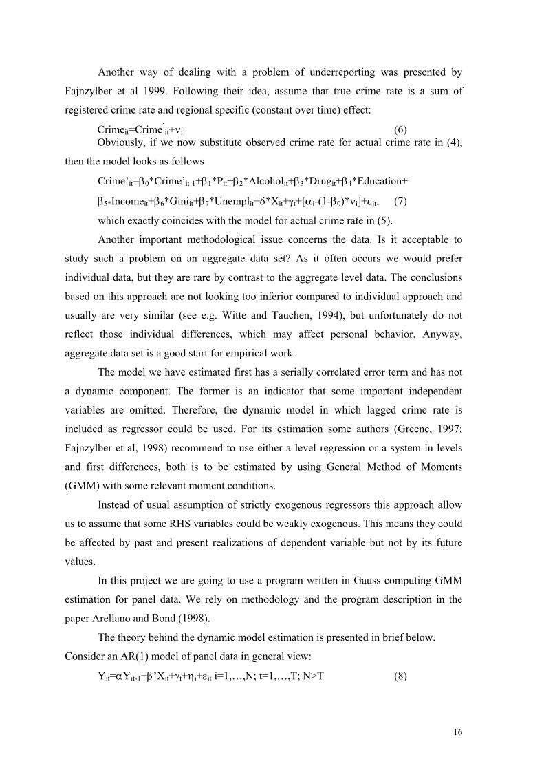
Another way of dealing with a problem of underreporting was presented by
Fajnzylber et al 1999. Following their idea, assume that true crime rate is a sum of
registered crime rate and regional specific (constant over time) effect:
Crimeit=Crime’it+νi (6)
Obviously, if we now substitute observed crime rate for actual crime rate in (4),
then the model looks as follows
Crime’it=β0*Crime’it-1+β1*Pit+β2*Alcoholit+β3*Drugit+β4*Education+
β5*Incomeit+β6*Giniit+β7*Unemplit+δ*Xit+γt+[αi-(1-β0)*νi]+εit, (7)
which exactly coincides with the model for actual crime rate in (5).
Another important methodological issue concerns the data. Is it acceptable to
study such a problem on an aggregate data set? As it often occurs we would prefer
individual data, but they are rare by contrast to the aggregate level data. The conclusions
based on this approach are not looking too inferior compared to individual approach and
usually are very similar (see e.g. Witte and Tauchen, 1994), but unfortunately do not
reflect those individual differences, which may affect personal behavior. Anyway,
aggregate data set is a good start for empirical work.
The model we have estimated first has a serially correlated error term and has not
a dynamic component. The former is an indicator that some important independent
variables are omitted. Therefore, the dynamic model in which lagged crime rate is
included as regressor could be used. For its estimation some authors (Greene, 1997;
Fajnzylber et al, 1998) recommend to use either a level regression or a system in levels
and first differences, both is to be estimated by using General Method of Moments
(GMM) with some relevant moment conditions.
Instead of usual assumption of strictly exogenous regressors this approach allow
us to assume that some RHS variables could be weakly exogenous. This means they could
be affected by past and present realizations of dependent variable but not by its future
values.
In this project we are going to use a program written in Gauss computing GMM
estimation for panel data. We rely on methodology and the program description in the
paper Arellano and Bond (1998).
The theory behind the dynamic model estimation is presented in brief below.
Consider an AR(1) model of panel data in general view:
Yit=αYit-1+β’Xit+γt+ηi+εit i=1,…,N; t=1,…,T; N>T (8)

17
A transformation (the first difference or orthogonal deviation) of this model is
applied in order to eliminate unobservable individual effect ηi. We will use the first
difference of the equation (8):
∆Yit=α∆Yit-1+β’∆Xit+∆γt+∆εit i=1,…,N; t=2,…,T; N>T (9)
where ∆Yit=Yit-Yit-1, ∆Xit=Xit-Xit-1 and so on..
If we assume, first, error term εit is not serially correlated, and, second,
explanatory variables are weakly exogenous, that is their current realization can be
determined only by past and current values of dependent variable, then the following
moment conditions can be used in GMM estimation:
E[Yit-s(γt+εit)]=0 for s≥1, t=2,…,T (10)
E[Xit-s(γt+εit)]=0 for s≥1, t=2,…,T (11)
As follows from both these conditions, E[Yit-s(∆γt+∆εit)]=0 for s≥2, t=3,…,T and
E[Xit-s(∆γt+∆εit)]=0 for s≥2, t=3,…,T which allows us to use second and higher lags of
dependent and weakly exogenous independent variables as instruments for the regression
in first differences.
Usually the regression in first differences (8) is complemented by the regression in
levels (9) as difference estimator has low asymptotic precision and large biases in small
samples. The instruments to be used for the regression in levels should not be correlated
with the individual effect ηi. Assuming stationary property of the model (7), that is
E[Yitηi]=E[Yisηi] and E[Xitηi]=E[Xisηi] for t=1,…,T; s=1,…,T we will have additional
moment conditions:
E[∆Yit-1(γt+ηi+εit)]=0 for t=3,…,T (12)
E[∆Xit-1(γt+ηi+εit)]=0 for t=3,…,T (13)
We see that lagged first differences of dependent and endogenous independent
variables could be used as instruments for the regression in levels, but further lags would
be redundant in the system estimation as lagged levels are already included as instruments
for the regression in first differences.
According Arellano and Bond (1991) GMM provide the next estimates for the
system of regressions (8) and (9) with moment conditions (10)-(13):
θ = ( ) yZZXXZZX ′Ω′′Ω′ −−− 111 ˆˆ (14)
Avar ( )θ = ( ) 11ˆ −− ′Ω′ XZZX (15)
18
where ( ),, βαθ = ( ),,1 XyX t−= ( ),,YYy ∆= Z is a special matrix constructed
from instruments, and Ω is a consistent estimate of variance-covariance matrix of the
moment conditions.
Crucial assumption for the consistency of estimators is no serial correlation of
error term εit. If it is not serially correlated, then its first difference εit-εit-1 should be
negatively first order serially correlated but not second order serially correlated. Formally,
Corr(εit-εit-1,εit-1-εit-2)=-σi2 and Corr(εit-εit-1,εit-2-εit-3)=0 if we assume Corr(εit,εit-1)=0 and
Corr(εit,εit)= σi2.
If the null hypothesis of no second order serial correlation is rejected then higher
order lags of dependent and endogenous independent variables should be used as
instruments. Another test in the model is a Sargan test of overidentifying restrictions,
which tests the validity of instruments. Not rejected null hypothesis supports the estimated
model.
Now we are ready to proceed further with econometric estimation of the model.
IV. Empirical part.
Note that in the theoretical framework we do not make any assumption on the type
of illegal activity. We think that the model is equally suited for both violent and property
crimes. In the former case, as it is often done in the neoclassic economic approach, we
assume that there are some psychic costs and gains from violent activity, which can be
evaluated in monetary terms. This approach is fruitful even in such a case, as we will see
later. The model (7) derived in the theoretical part will be estimated for both violent (or
personal) and property crimes. Though criminologists may object to this approach and
call different causes for each particular type of crime, we believe that we are using factors
common for either crime activity. Also, this approach allows us to assess the possible
substitution effect between two types of crime.
Violent crimes in Russian juridical literature include the four types of crime,
namely homicide, assault, rape, and hooliganism. The number of homicides and attempted
homicides will be used as a proxy for violent crime rate11. According to criminologists,
this indicator has the highest quality as it better reported by police. On the contrary, the
number of larceny-thefts, which we are using as a proxy for property crime rate suffers
11 They total about 15 % of all violent crimes in Russia.

19
from underreporting12 though it presents the largest part of property crimes13. The most
frequent types of crimes against property are larceny-theft, burglary, robbery, fraud, and
auto-theft.
IV.i. Data.
Descriptive statistics and definition of variables are presented in Tables 1 and 2 in
Appendix. Note that economic indicators have quite large standard deviations. It is not
strange inasmuch as moderate differences in initial conditions and further economic crises
and divergence of the Russian regions.
Crime levels and clear-up ratios both for homicide and larceny for all 89 regions in
1990-1998 were provided by the Main Information Center of the Russian Federation
Ministry of the Interior in which all statistics about crime in the country are collected. A
regional map of homicide rate per 100’000 population in 1998 can be found in Appendix,
Figure 1. Some shortcomings of official crime levels were already discussed above.
Alcohol consumption figures are not available for regions and even for Russia as a
whole. We know, however, official and shadow production of vodka, which total about 7
litters of pure alcohol per capita in 1999 (Goscomstat, 2000)14. Following the
recommendations of an expert15, the best available proxy for alcohol consumption could
be the number of people hospitalized in stationary medical facilities with alcoholic
psychosis, and to some extent a mortality rate from alcohol poisoning16. The former was
obtained from the Institute of Narcology for 80 regions over the period of 1990-1998 and
the latter is from the Institute of Psychiatry for 89 regions over the period of 1991-1998.
Unfortunately, none of the above alcohol indicators reflect the picture of alcohol
consumption accurately, especially in rural areas, where men are usually heavy drinkers
and are not treated for alcoholism. The national homicide and alcohol psychosis rates are
shown on Figure 2 in Appendix.
12 About 80 % of them are not reported and not registered by police. 13 About three fourth of all property crimes. 14 Nevertheless, different estimates of alcohol consumption in Russia at the end of 90-es show the level of about 14 liters of absolute alcohol per capita a year (e.g. Izvestiya, Jan 5, 2000). 15 Professor Nemtsov from the Institute of Psychiatry, Moscow, who is an author of papers on alcohol addiction issues. 16 Simply because they are better reported and reflect more or less plausibly the share of people who heavily consume alcohol drinks. But alcohol-poisoning mortality is looking inferior proxy to alcohol psychosis as it reflects quality rather than quantity of consumed beverages.

20
Drug consumption was approximated by the number of people with diagnosed
drug addiction, which was also obtained from the Institute of Narcology for all Russian
regions during the period 1991-1998. Although the real number of drug users is
not less than ten times as much as this official statistics reports17, we hope that data
correctly reflect dynamics and differences among the regions, i.e. we assume that
proportion of registered drug users is somehow stable over time but different only for
each region. Data for 1990 was extrapolated.
Real income is calculated at constant prices of 1990. Nominal income per capita
for 1990-1993 was obtained from Goscomstat (1999). Average annual CPI for 1991 and
1992 obtained from Goscomstat (1994) and 1993 obtained from the RECEP database
were used as price deflators. Real income per capita for the other years was calculated
from real income growth for 1994-1998 taken from Goscomstat (1999). These figures are
available only for 70 Russian regions.
The Gini coefficient for 1994-1998 was produced by the author’s calculations
based on data from Goscomstat (1999). Assuming lognormal distribution of income in the
regions and implementing the two-factor model, the coefficient was calculated based on
the subsistence level, average income and the share of population with income below the
subsistence level. For the other years coefficient was extrapolated, assuming that income
inequality was not greater in 1990-1993 than it in 1994.
The level of education is again the author’s calculations of average years of
schooling of population above fifteen years of age. Distribution of population by
educational level is from Micro census (1995). Figures for the other years were
propagated. The share of indigenous population in the region representing ethnic structure
in this study was obtained from the last census of population (Census, 1989) and it is also
constructed to be stable over time.
Other demographic indicators, a share of urban and a share of young population
(below 16 years of age) in a region for 1990-1998 (Goscomstat, 1999) could be the
important demographic variables. The indicators of geographical location of the region
are presented by the latitude and longitude of the regional center. They are another pair of
constant in time indicators.
Family disruption in our paper is measured by the difference between the number
of marriages and divorces in a region (Goscomstat, 1999).
17 Official number of people with diagnosis of drug addiction was 155 thousand while narcology specialists estimate the real number of drug users is over 3 million people.
21
The number of unemployed people is taken from Goscomstat annual labor force
survey (Goscomstat 1999), which is conducted regularly since 1992 and uses a standard
ILO classification. Data for proceeding years were obtained by extrapolation.
IV.ii. Regression results.
Regressions were run in the program DPD98 written by mentioned above Arellano
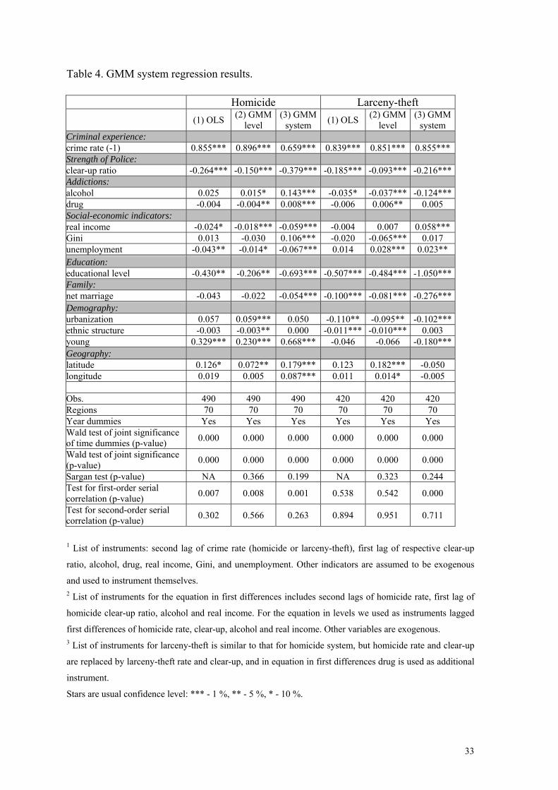
and Bond (1998), which was kindly provided by Hartmut Lehmann. In Table 4 in
Appendix we report the results of three regressions, first for homicide rate and then for
larceny-theft. The table presents average elasticities of the crime rate with respect to
independent variable. Elasticities were calculated from the obtained coefficient estimators
multiplied by the ratio of dependent and independent variable means. Definitions of
variables and their descriptive statistics can be found in Tables 1 and 2 respectively.
The OLS estimators of model (7) without dynamic term, i.e. when lagged crime
rate is not included as explanatory variable, are not valid since test for no first-order serial
correlation is rejected and therefore they are not reported in Table 4.
First column is a simple OLS estimation of the model (7). The second is GMM
estimation of the regression in levels, i.e. the model (7) with the list of instruments, which
includes second lag of crime rate and first lags of weakly exogenous explanatory
variables. The third is a system GMM estimation of the regression (7) and its first
difference with lagged differences and second lags of levels used as instruments for the
equations in levels and first differences respectively. Here we use two-step procedure to
obtain efficient and consistent estimates, which explores residuals from the first step to
construct the consistent estimate of variance-covariance matrix.
Sargan test of overidentifying restrictions under the null hypothesis of the validity
of instruments is not rejected for all four GMM estimations. The disturbances from all
three regressions for homicide and the third regression for larceny-theft are not serially
correlated as the test for no first-order serial correlation of differenced residuals is rejected
and test for no second-order serial correlation is not rejected. OLS and GMM level
regressions for larceny-theft are not valid, as they have autocorrelated residuals what
probably reflects that there are some important omitted variables.
We are going to ground our conclusions on GMM system estimation since it is
more efficient and controls for likely endogeneity of explanatory variables. However,
22
from Table 4 we can conclude that all three valid regressions for homicide show striking
similarity in results, with only some exceptions for homicide regressions.
Note that we have observation for transition period from 1990 to 1998 and sample
period for GMM includes 7 last years for homicide system of regressions and 6 years for
case of larceny-theft, whereas 2 first years are used as instruments. Also, another
assumptions for consistency of estimation, that N is greater than T (70>9) and N is
(asymptotically) large, are satisfied.
We can conclude that both homicide and larceny rates are persistent over time.
The lagged dependent variable, which is a proxy for criminal experience is very
significantly positive. Its elasticity is equal to 0.66 in case of homicide and 0.86 for
larceny-theft. As we could predict thieves are more likely to repeat an offence than
murderers and this is reflected in larger elasticity. Therefore, we can expect that
homicides are more closely connected with other indicators. Although the interpretation
of the past crime level as criminal experience could be restricted and in reality it is more
complex, we think, it already contains all other information, that is accommodated to
changes in its determinants.
The strength of Police, measured by the proportion of solved crimes (detection
rate) is significantly negative in both cases. A higher share of cleared crimes may have
two effects. The first one is a so-called incapacitation effect when criminals in custody are
not able to continue their criminal activities (among freeside people) while they are in jail,
thereby decreasing the number of offenders who are free. The second is a deterrence
effect, which means that a higher probability of not getting away with a crime is
preventing some people (criminals or not) from getting involved in crime industry. Since
most studies show a negligible size of incapacitation effect, further we will refer to clear-
up ratio as a deterrent effect of Police on crime. Therefore, the deterrent effect arising
from police activity is found to be playing the essential role in determination of current
incidence of any crime activity. This indicates the importance of this factor despite its
imperfection in measuring on the first glance, given the large share of not registered
crimes, especially for larceny-theft.
The next scope of socio-economic indicators has surprisingly opposite impact on
violent and property crimes. While higher alcohol consumption increases violence, it has
the opposite effect on property crimes. This confirms a statistical evidence of high share
of violent crimes committed by alcohol-intoxicated people. Effect on property crime is
not strange as the share of crimes committed by drunk offenders is much lower in this
23
case and do not exceed 20 % at the end of 90-es, while alcohol played not the last role in
not less than 70 % of violent cases. As observed in developed countries, alcohol
consumption is counter-cyclical in Russia, i.e. rises during economic recession. Another
important cause of increased alcohol consumption was lost state monopoly on alcohol
production in 1992 and as a consequence, low price and abundance of low quality
counterfeit alcohol, which led to sharp rise in alcohol consumption entailing a higher rate
of fatal alcohol poisoning. Fortunately, from 1995 alcohol consumption was declining at
least up to the crisis in August 1998, following which it seems to be rising again18.
Besides the number of alcohol psychosis we tried mortality rate from alcohol poisoning as
another proxy for alcohol consumption. In this case alcohol continue to have significant
increasing effect on homicides. At the same time, higher drug consumption significantly
raises either types of crime. In spite of this finding, the Ministry of Interior statistics
reports still very low but rising share of crimes committed under the influence of drug,
which may reflect the fact that a narcotist usually commit a crime before drug usage in
contrast to offenders who prefer alcohol. The close relationship between drug
consumption and property crime is expected given that drugs are very expensive and a
typical drug user is a relatively poor young person19.
Poverty is another important factor of crime. According to the regression results,
the rise in real income causes the fall in violent activity of criminals and the rise in
acquisitive crime. A negative income effect on crime was clearly observable after the
1998 crisis when real income suddenly fell drastically by 30 %, which was followed by an
approximately 25 % rise in crime rate during the next year. That year saw also an
especially strong rise in larceny-theft, about 34 %, what is not corresponding to our results
and probably was connected not with income but rather with other reasons like increased
number of crimes committed by a theft or sudden rise in reporting rate.
On the other hand, we can conclude that higher income inequality measured by
Gini index leads to higher violence20 but have no significant effect on thefts. Meanwhile,
income inequality is a measure of social tension in the society. More tension means more
conflicts in social groups, including family, and hence more violence.
People who are unemployed, especially for a long time and with low chances to
find a job are thought to be more prone to illegal activities due to low opportunity costs,
18 Undoubtedly this is a feature of Russian crises. 19 Say, the doze of heroin in Moscow is about five times as expensive as a bottle of vodka. 20 What other researchers observe in different countries.

24
that is legal earnings. The Ministry of Justice statistics report that during transition the
share of convicted people without a permanent source of income rose from 16 to 55 %.
But does this mean that criminals constitute the largest part among unemployed? Probably
not because criminals are usually young people without working experience and with low
chances to find a legal job with comparable income. Therefore, they are not in the labor
force. While the results of studies in other countries do not show a clear relationship
between crime and unemployment, some evidence of a positive relationship exists. Our
results show that unemployment rise is associated with lower violence but higher property
crime cases.
Educational level is measured as average years of schooling of people above 15
years of age according to the Micro Census 1994. An impact of education on crime is
recognized as ambiguous in the economic literature. It may cause some opposite effects.
On the one hand, a higher level of education might indicate higher moral norms and
greater job opportunities resulting in higher income in the legal economy. On the other
hand, such people may be even smarter and more productive in some types of illegal
activities and therefore, have higher gains from that. Regression results support the first
idea, showing strong significant negative impact of educational attainment on both types
of crime. Have people in a region on average one additional year of schooling, either
crime rates will be about 8-11 per cent lower. Possibly reporting rate will be higher in this
case thereby increasing even more the found effect of education on crime.
Concerning demographical indicators, urbanization of a region is better for
property crime that is the more urban a region the less registered crime rates. Note that in
a simple correlation analysis crime rate is higher in more urban areas, the picture exactly
observed in other countries, e.g. in USA. From the correlation matrix in Tables 5 and 6 in
Appendix we see that for homicide rate significantly negatively correlated indicators are
clear-up and net marriage, and for larceny – clear-up, Gini index, net marriage and ethnic
structure.
Another demographic indicator, presenting age structure is differently signed.
Regions with larger share of young population suffer from higher violence but gain from
lower property crimes. This conclusion is correspondent with mentioned above age
structure of people convicted in crime.
Geographical and demographical indicators are also significant in the GMM
regressions. As it looks on the map of Russian regions in Appendix, where homicide rate
is increasing from west to east and from south to north, the regressions provide the same

25
conclusion. Namely, after controlling for crime experience, the strength of police and the
set of socio-economic-demographic indicators, latitude and longitude continue to be
significantly positive for homicide rate, reflecting other unobserved or not controlling
differences among the regions (like climate, daytime, and possibly culture, traditions,
norms, etc). But for larceny-theft both indicators are not significant. That gives support to
the idea that regional differences in natural indicators like temperature and duration of
nighttime could be important crime factors leading to more conflicts within family and
neighborhood.
Not less interesting conclusion is that crime rates are closely related with main
socio-economic indicators. More importantly, during crises when alcohol consumption
and income inequality rise and real income falls we observe substitution of property
crimes by violent crimes. In reality both crime rates were rising after shocks and crises in
1992 and 1998 and this was probably caused by problems with Police force financing
inadequate to new conditions, what led to lower detection rate. This fact slightly hides the
clearness of our findings about substitution effect. But it seems that after crisis, when
violence was rising, a large part of Police resources was sent on fighting with violent
offenders, thus giving more incentives to other crime activities.
Another important observation is a rather small magnitude of estimated elasticities
of socio-economic indicators. Therefore, only large changes in economic conditions could
be followed by considerable changes in criminal activity. This is exactly what Russia has
experienced during 90-es and is also true for period of gradual crime growth during long
period from 60-es to 80-es. Thus, say, twofold fall in real income is followed by only 6
per cent rise in crime rate according to our estimates.
Robustness check of obtained results was done in the following directions. First,
as we already note, even if we use other estimation technique like pooled OLS and GMM
in level for homicide, results are similar though inefficient. Second, we restricted data
sample on the regions in the European part of Russian Federation. For this sub sample we
had to narrow the list of instruments for the regression in levels as the previous set is not
working and making the program to abort. However, the main conclusions do not change
with the exception of real income and Gini, which lost their significance, maybe due to
incorrect list of instruments. Third, we used other time periods, like 1993-1998 and 1994-
1998. In these cases basic results remain the same with minor changes. Thus, for
homicide only drug consumption has become significantly negative and for larceny real
income and unemployment have lost their significance, what may be caused by a short

26
time period. And fourth, trying to cope with collinearity problems, we restricted the set of
regressors on the core list, which includes criminal experience, strength of Police, alcohol
and drug consumption, and three socio-economic indicators. In this case all results remain
with two exceptions. First, detection rate for thefts continues to be negative but not highly
significant. Second, unemployment rate becomes significantly positive for violence. As
the last step in this model specification we study robustness of opposite effects on crime
from income and income inequality. There is a significant positive correlation between
real income and Gini coefficient, from the Table 5 it is equal 0.4. Real income was
replaced by the interactive term between real income and Gini coefficient. As a result, we
have found a further confirmation of increasing effect of inequality on violent crimes. But
at the same time interactive term is significantly negative, implying that real income
growth with unchanged income distribution leads to reduction in violence.
All checks we have made allow us to consider obtained results as being quite robust.
V. Policy implications.
Both violent and property crimes in Russia have a high degree of criminal inertia,
which can be explained by correspondent level of criminal experience and its spreading. It
may sound strange for usually not repeated crimes like homicides and more suited for
recidivism in property crimes. Anyway, our finding tells us that there is a stable social
environment, which may be called “social illness”, that generates a deviant behavior of
some part of population. Under stable environment we mean rather stable demographical
and geographical situation, educational attainment, everything not connected directly with
economic situation. This environment could from our point of view almost entirely
explain differences in crime levels and long-term changes in crime situation. Say,
observed fall in birthrate during 90-es leads to decreasing share of young people and
therefore in less violence in couple decades. The similar positive impact is expected from
higher educational level. One additional year of education decreases crime level by about
10 per cent. Economic situation should have immediate effect on crime, but this effect is
found to be surprisingly very low. Other indicators closely related with economic
situation, like alcohol consumption, family formation and disruption have higher order
impact on crime levels. Only these indicators among studied have considerable short-term
effect. Moreover, we still do not know what are other major reasons of short-term crime
growth. Direct short-term effect from economic improvement unfortunately does not
27
show less crime activity. Say, Russia had outstanding 7 % GDP growth in 2000, while
total crime rate has fallen by only 2 % at that year.
Present conditions of Russian penal system only facilitate the transfer of criminal
experience to convicted or suspected young persons. Policy makers should have in mind
this fact before this system will be reformed. Efficiency of law enforcement activity is
very restricted and even if detection rate rises by 20 % (say from 50 to 60%), ceterus
paribus, crime will fall only by 5-7 %. We have to think now what is better for the
country, to finance Police and build new prisons or invest more in education and
economy, or help families. The first is undoubtedly much cheaper but do not solve a
problem and have miserable effect.
As for families, we would like to note here how important (not only from
criminological but demographical view) to help young people to form a family and split
those families, which are not able to live together. On the one hand, a family prevents
young man from theft and other criminal activity. On the other hand, obstacles for
divorces in unhappy families often lead to deplorable consequences, especially in those
families, where husbands drink to excess.
In the long run we could expect that once Russia has sustained growth, violent
crimes will be decreasing (say, homicide rate will decline together with other mortality
indicators) as we can judge from our results. No doubt that Criminal Justice System has to
be reformed because it could prevent further crime growth in Russia at some extent, but
only if its development will be adequate to new conditions. Increasing level of education
for young people can be resulted in their lower involvement in illegal activity today while
they are studying and in future when they will be working. In this respect twelve years of
secondary education is a good reform of education in Russia, which will improve the
crime situation. And this is good news. But there is bad news. With higher drug
consumption Russia will probably have further rise in either crimes. With better economic
conditions violent crimes will be replaced by acquisitive crimes, what we observe now in
developed countries. Higher income and unemployment rate could lead to more property
crimes. The remedies that can prevent this rise in property and economic crimes exist
maybe outside the economic sphere. From these facts we can sum up, that crime is a price
paid for open society and growth.

28
References.
In Russian:
I. Statistical books:
Goscomstat, 1994, «Индексы цен в России, 1990-1992 гг.», Москва, Госкомстат.
Goscomstat, 1999, «Российский статистический ежегодник», Москва, Госкомстат.
Goscomstat, 2000, «Социально-экономическое положение в Российской Федерации», 1,
2000, Москва, Госкомстат.
Household survey, 1997, «Статистический бюллетень», …, Москва, Госкомстат.
Москва, Госкомстат.
Household survey, 1998, «Статистический бюллетень», …, Москва, Госкомстат.
II. Literature:
Becker, 1968, Беккер Г., «Преступление и наказание: экономический подход», Истоки 4,
Москва, 2000, с. 28-90.
Climate, 1997, «Предпринимательский климат регионов России: география России для
инвесторов», Москва, Начала-Пресс.
Criminology, 1999, «Криминология. Учебник для юридических вузов», СП-б.: Санкт-
Петербургский университет МВД России.
Entorf, 1997, Энторф Х., «Преступность с экономической точки зрения: факты, теория и
статистика», Политэконом, 1, 1997.
Kudryavtsev, 1999, Кудрявцев, В. Н., «Современные проблемы борьбы с преступностью в
России», Вестник Российской академии наук, том 69 9, с. 790-797.
Latov, 2000, Латов Ю.В., «Экономика преступлений и наказаний: тридцатилетний юбилей»,
Истоки 4, Москва, 2000, с. 228-270.
Micro census, 1995, «Образование населения России: по данным микропереписи населения
1994 года», Москва, Госкомстат, 1995.
Survey, 1991, «Мнение населения о правовой защищенности и деятельности
правоохранительных органов в Российской Федерации», Государственный комитет по
статистике Российской Федерации, Москва, РИИЦ, 1992.
Census, 1989, «Некоторые итоги Всесоюзной переписи населения 1989 года», Москва,
Госкомстат, 1991.
Sinelschikov, Синельщиков, 1998, «Лукавые цифры милицейской статистики. Преступность
снижается только на бумаге», http://besta.rbc.ru/documents/vek/980203/0231303.html.

29
In English:
Arellano, M. and S. Bond (1991), “Some tests of specification for panel data: Monte Calro
evidence and an application to employment equations”, Review of Economic Studies 58, 277-297.
Arellano, M. and S. Bond (1998), “Dynamic Panel Data Estimation Using DPD98 for Gauss: a
Guide for Users”.
Avio, K.L. and C.S. Clark, 1976, “Property crime in Canada: an econometric study”, Ontario
Council Economic Research Studies, Ontario, Canada.
Becker, Gary, 1968, “Crime and Punishment: An Economic Approach”, Journal of Political
Economy 76: 169-217.
Becker, Gary, 1995,”The Economics of Crime”, reprint from the Fall 1995 issue of Cross
Sections, a publication by the Federal Reserve Bank of Richmond,
http://www.rich.frb.org/cross/pubs/crime1.html.
Blustein, A., J. Cohen and D. Nadin, eds, 1978, “Deterrence and incapacitation: estimating the
effect of criminal sanctions on crime rate”, National Academy of Sciences, Washington, D.C.
Danziger, S. and D. Wheeler, 1975, “The economics of crime: punishment or income
distribution”, Rev. Soc. Econ., 113-31.
Ehrlich, Isaac, 1973, “Participation in Illegitimate Activities: A Theoretical and Empirical
Investigation”, Journal of Political Economy 81: 521-565.
Eide, Erling, 1994, “Economics of Crime. Deterrence and the Rational Offender”, Contribution to
economic analysis, # 227, North-Holland.
Fajnzylber, Pablo, Lederman, Daniel, and Loayza, Norman, 1998, “What Causes Violent
Crime?”, Office of the Chief Economist Latin America and the Caribbean, The World Bank,
mimeo.
Fajnzylber, Pablo, Lederman, Daniel, and Loayza, Norman, 1999, “Inequality and Violent
Crime”, Office of the Chief Economist Latin America and the Caribbean, The World Bank,
mimeo.
Fleisher, Belton, 1966, “The Effect of Income on Delinquency”, American Economic Review, 56:
118-137.
Forst, B., 1976, “Participation in illegitimate activities: further empirical findings”, Policy Anal.,
2, 3, 477-92.
Greene, W., 1997, ”Econometric Analysis”, Prentice-Hall.
Griliches, Zvi and Hausman, Jerry, 1986, “Errors in Variables in Panel Data”, Journal of
Econometrics 31: 93-118.
Heineke, J.M., 1978, Economic models of criminal behaviour. Amsterdam, North-Holland.
Holtman, A.G. and L. Yap, 1978,”Does punishment pay?” Pub. Fin., 33, 1-2, 90-7.
30
Imrohoroglu, Ayse; Merlo, Antonio; Rupert, Peter, 1996, “On the Political Economy of Income
Redistribution and Crime”, Federal Reserve Bank of Minneapolis Staff Report: 216, September
1996, p.35.
Lenke, L., 1975, “Violent Crime and Alcohol: A Study of the Developments in Assaultive
Crime”, Stockholm, Department of Criminology, University of Stockholm.
Levitt, Steven, 1995, “Why Do Increased Arrest Rates Appear to Reduce Crime: Deterrence,
Incapacitation, or Measurement Error?”, NBER Working Paper No.5268.
Levitt, Steven, 1997, “Using Electoral Cycles in Police Hiring to Estimate the Effect of Police on
Crime”, American Economic Review, 81(3), June 1997, p. 270-290.
Markowitz, Sara, 2000, “Criminal Violence and Alcohol Beverage Control: Evidence from an
International Study”, NBER Working Paper #7481.
Mathieson, D. and P. Passell, 1976, “Homicide and robbery in New York city: an econometric
model”, J. Legal Stud., 5, 83-98.
Myers, S.L., 1980, “Why are crimes underreported? What is the crime rate: does it really matter?”
Soc. Sc. Q., 61, 1 (June), 23-43.
Mathur, V.K., 1978,”Economics of crime: an investigation of the deterrent hypothesis for urban
areas”, Rev. Econ. Stat., 60, 3 (Aug), 459-66.
Sjoquist, D., 1973, “Property crime and economic behavior: some empirical results”, Am. Econ.
Rev., 63, 3, 439-46.
Swimmer, E.R., 1974, “Measurement of the effectiveness of urban law enforcement – A
simultaneous approach”, Southern Econ. J., 40, (April), 618-30.
Thaler, R., 1977, ”An econometric analysis of property crime”, J. Pub. Econ.,8, 323-38.
Vandaele, W., 1978, “Participation in Illegitimate activities: Ehrlich revised”, in Blumstein et al.,
270-335.
Willis, K.G., 1983, “Spatial variations in crime in England and Wales: testing an economic
model”, Reg. Stud., 17, 4, 261-72.
Witte, Ann and Tauchen, Helen, 1994, “Work and Crime: An Exploration Using Panel Data”,
NBER Working Paper No. 4794

31
Appendix.
Table 1. Description of the variables used in the regressions.
Variable Description Homicide rate Number of homicides per 100'000 population Larceny rate Number of larceny-thefts per 100'000 population Clear-up ratio Proportion of homicides (larceny-thefts) solved by Police
Alcohol consumption Number of people hospitalized to stationary medical facilities with diagnosis of alcohol psychosis per 100'000 population
Drug consumption Number of registered people with diagnosis of drug addiction, per 100'000 population
Real income Average income in constant 1990 prices Gini index Income inequality measure, from 0 to 100 Unemployment Unemployment rate, per cent Educational level Average years of schooling of population above 15 years of age
Net marriage Number of marriages minus number of divorces, per 1'000 population
Urban population Share of urban population, per cent Ethnic population Share of indigenous (non-Russian) population, per cent Young population Share of young population below 16 years of age, per cent Latitude Geographical latitude Longitude Geographical longitude

32
Table 2. Descriptive statistics for the homicide regression.
Variable Obs. Regions Mean Std Dev Min Max Homicide rate 490 70 19.611 8.880 3.655 79.085 Clear-up ratio 490 70 80.543 10.017 22.200 94.200 Alcohol consumption 490 70 79.270 40.299 0.500 220.700 Drug consumption 490 70 49.335 57.587 2.100 372.100 Real income 490 70 149.488 80.815 35.000 628.000 Gini 490 70 34.131 6.267 16.913 60.109 Unemployment 490 70 9.814 4.693 2.800 30.800 Education level 490 70 9.373 0.473 8.681 11.107 Net marriage 490 70 2.571 0.916 -0.700 6.900 Urban population 490 70 70.320 11.612 36.957 100.000 Ethnic population 490 70 9.133 19.505 0.000 80.200 Young population 490 70 23.524 3.477 17.200 36.800 Latitude 490 70 54.643 5.286 43.000 68.000 Longitude 490 70 59.543 34.280 21.000 162.000 Table 3. Descriptive statistics for the larceny-theft regression.
Variable Obs. Regions Mean Std Dev Min Max
Larceny rate 420 70 904.244 333.276 153.031 2241.597 Clear-up ratio 420 70 49.279 11.131 18.700 83.500 Alcohol consumption 420 70 85.917 39.012 0.500 220.700 Drug consumption 420 70 53.984 59.947 2.200 372.100 Real income 420 70 150.519 83.908 35.000 628.000 Gini 420 70 34.042 6.233 16.913 60.109 Unemployment 420 70 10.592 4.585 3.300 30.800 Education level 420 70 9.373 0.473 8.681 11.107 Net marriage 420 70 2.523 0.887 -0.700 6.300 Urban population 420 70 70.245 11.670 36.957 100.000 Ethnic population 420 70 9.133 19.508 0.000 80.200 Young population 420 70 23.304 3.423 17.200 36.500 Latitude 420 70 54.643 5.287 43.000 68.000 Longitude 420 70 59.543 34.286 21.000 162.000
33
Table 4. GMM system regression results.
Homicide Larceny-theft
(1) OLS (2) GMM level
(3) GMM system (1) OLS (2) GMM
level (3) GMM
system Criminal experience: crime rate (-1) 0.855*** 0.896*** 0.659*** 0.839*** 0.851*** 0.855*** Strength of Police: clear-up ratio -0.264*** -0.150*** -0.379*** -0.185*** -0.093*** -0.216*** Addictions: alcohol 0.025 0.015* 0.143*** -0.035* -0.037*** -0.124*** drug -0.004 -0.004** 0.008*** -0.006 0.006** 0.005 Social-economic indicators: real income -0.024* -0.018*** -0.059*** -0.004 0.007 0.058*** Gini 0.013 -0.030 0.106*** -0.020 -0.065*** 0.017 unemployment -0.043** -0.014* -0.067*** 0.014 0.028*** 0.023** Education: educational level -0.430** -0.206** -0.693*** -0.507*** -0.484*** -1.050*** Family: net marriage -0.043 -0.022 -0.054*** -0.100*** -0.081*** -0.276*** Demography: urbanization 0.057 0.059*** 0.050 -0.110** -0.095** -0.102*** ethnic structure -0.003 -0.003** 0.000 -0.011*** -0.010*** 0.003 young 0.329*** 0.230*** 0.668*** -0.046 -0.066 -0.180*** Geography: latitude 0.126* 0.072** 0.179*** 0.123 0.182*** -0.050 longitude 0.019 0.005 0.087*** 0.011 0.014* -0.005 Obs. 490 490 490 420 420 420 Regions 70 70 70 70 70 70 Year dummies Yes Yes Yes Yes Yes Yes Wald test of joint significance of time dummies (p-value) 0.000 0.000 0.000 0.000 0.000 0.000
Wald test of joint significance (p-value) 0.000 0.000 0.000 0.000 0.000 0.000
Sargan test (p-value) NA 0.366 0.199 NA 0.323 0.244 Test for first-order serial correlation (p-value) 0.007 0.008 0.001 0.538 0.542 0.000
Test for second-order serial correlation (p-value) 0.302 0.566 0.263 0.894 0.951 0.711
1 List of instruments: second lag of crime rate (homicide or larceny-theft), first lag of respective clear-up
ratio, alcohol, drug, real income, Gini, and unemployment. Other indicators are assumed to be exogenous
and used to instrument themselves. 2 List of instruments for the equation in first differences includes second lags of homicide rate, first lag of
homicide clear-up ratio, alcohol and real income. For the equation in levels we used as instruments lagged
first differences of homicide rate, clear-up, alcohol and real income. Other variables are exogenous. 3 List of instruments for larceny-theft is similar to that for homicide system, but homicide rate and clear-up
are replaced by larceny-theft rate and clear-up, and in equation in first differences drug is used as additional
instrument.
Stars are usual confidence level: *** - 1 %, ** - 5 %, * - 10 %.

34

35
Table 5. Correlation matrix for the homicide regression. (1) (2) (3) (4) (5) (6) (7) (8) (9) (10) (11) (12) (13) (14) (15) (1) Homicide rate 1.00 (2) Lagged homicide rate 0.94 1.00 (3) Clear-up ratio -0.11 -0.09 1.00 (4) Alcohol consumption 0.13 0.13 -0.05 1.00 (5) Drug consumption 0.36 0.41 -0.22 -0.12 1.00 (6) Real income 0.03 0.01 -0.09 0.38 -0.07 1.00 (7) Gini 0.25 0.25 -0.26 -0.01 0.25 0.34 1.00 (8) Net marriage -0.12 -0.15 -0.18 -0.48 -0.07 -0.22 0.17 1.00 (9) Unemployment 0.18 0.26 -0.16 -0.11 0.37 -0.26 -0.04 0.01 1.00 (10) Latitude 0.11 0.10 0.34 0.44 -0.27 0.48 0.01 -0.48 -0.23 1.00 (11) Longitude 0.53 0.52 0.06 -0.05 0.27 0.05 0.05 -0.31 0.03 0.09 1.00 (12) Urban population 0.00 -0.01 -0.19 0.48 -0.05 0.36 0.05 -0.60 -0.24 0.48 0.13 1.00 (13) Ethnic population 0.17 0.18 -0.18 -0.38 0.05 -0.18 0.03 0.53 0.38 -0.28 -0.03 -0.47 1.00 (14) Education level 0.22 0.21 -0.45 0.15 0.23 0.40 0.31 -0.35 0.02 0.20 0.42 0.59 -0.01 1.00 (15) Young population 0.45 0.42 -0.05 -0.40 0.12 -0.03 0.15 0.37 0.16 -0.15 0.41 -0.48 0.65 0.08 1.00 Table 6. Correlation matrix for the larceny-theft regression. (1) (2) (3) (4) (5) (6) (7) (8) (9) (10) (11) (12) (13) (14) (15) (1) Larceny-theft rate 1.00 (2) Lagged larceny-theft rate 0.93 1.00 (3) Clear-up ratio -0.55 -0.57 1.00 (4) Alcohol consumption 0.27 0.29 -0.21 1.00 (5) Drug consumption -0.03 -0.02 0.05 -0.22 1.00 (6) Real income 0.01 0.04 -0.29 0.41 -0.08 1.00 (7) Gini -0.18 -0.11 -0.19 0.00 0.26 0.38 1.00 (8) Net marriage -0.45 -0.44 0.03 -0.47 -0.06 -0.19 0.17 1.00 (9) Unemployment -0.22 -0.24 0.32 -0.33 0.32 -0.31 -0.04 0.06 1.00 (10) Latitude 0.33 0.31 -0.23 0.48 -0.26 0.47 0.01 -0.48 -0.25 1.00 (11) Longitude 0.40 0.42 -0.28 -0.06 0.28 0.02 0.07 -0.32 0.03 0.09 1.00 (12) Urban population 0.19 0.19 -0.25 0.53 -0.05 0.37 0.05 -0.59 -0.27 0.48 0.13 1.00 (13) Ethnic population -0.34 -0.30 -0.03 -0.43 0.04 -0.18 0.03 0.52 0.43 -0.28 -0.03 -0.47 1.00 (14) Education level 0.03 0.07 -0.35 0.16 0.24 0.41 0.31 -0.33 0.01 0.20 0.42 0.59 -0.01 1.00 (15) Young population 0.03 0.07 -0.31 -0.37 0.15 -0.05 0.16 0.37 0.25 -0.17 0.40 -0.50 0.67 0.07 1.00

36
Figure 1.

37
Figure 2.
Homicides and alcohol consumption, 1985-1999
0
5
10
15
20
25
1985
1986
1987
1988
1989
1990
1991
1992
1993
1994
1995
1996
1997
1998
1999
0
25
50
75
100
125
150
Homicides and attempedhomicides, per 100'000population (left scale)Real alcohol consumptionfrom monthly data,10=1992 (left scale)No. Of alcohol psychosisper 100'000 population(right scale)