Explaining and Forecasting Inflation in Turkey*

by

Ilker Domaç

July 2003

The growing adoption of inflation targeting (IT) framework in emerging market economies has increased the importance of understanding inflation dynamics and forecasting its future path in these countries. This paper considers the case of Turkey and investigates the performance of models that have some theoretical foundations. To this end, the study focuses on mark-up models, monetary models, and the Phillips curve. The findings suggest that the mark up models have the best in-sample performance followed by money gap models and the Phillips curve. The empirical results from out-of-sample forecasting performance for the period covering the new economic program (May 2001-December 2002), however, show that the Phillips curve and the money gap models perform better than mark-up models. These findings, in turn, imply that (i) Phillips curves augmented with the exchange rate and money models might provide complementary views in the Turkish context; and (ii) the relative importance of output gap and monetary disequilibrium in the inflation process has increased under the floating exchange rate regime. All in all, the results underscore the importance of relying on multiple models of inflation in the conduct of Turkish monetary policy.

JEL classification: E31; E37; E58; C53

* I would like to thank Mark Griffiths for his helpful comments and Mustafa Eray Yücel for his valuable assistance. The findings and conclusions of the paper are solely those of the author and not necessarily those of the Central Bank of Turkey.

Why is our money ever less valuable? Perhaps it is simply that we have inflation because we expect inflation, and we expect inflation because we’ve had it.

—Robert M. Solow1 1. Introduction

Contrary to many emerging market economies, which have experienced

noticeable declines in inflation owing to a combination of relatively favorable external

factors and implementation of sound domestic policies, Turkey is still endeavoring to

curb chronic high inflation and attain price stability (Table 1). The absence of a

permanent fiscal adjustment coupled with unsatisfactory progress with the

implementation of key structural reforms lie at the heart of the chronic high inflation in

Turkey. The experiences from a variety of approaches to stabilization adopted by

emerging market economies (exchange rate-based orthodox programs and heterodox

programs) also confirm that inflation does not stay permanently low in the absence of a

permanent fiscal adjustment.2

Table 1. Evolution of the Inflation Rate in Selected Emerging Market Economiesa 1981-1990 1991-1995 1996-2000 2000 2001 2002Turkey 46.3 79.3 74.1 54.9 54.4 45Israel 118.3 12.9 6.4 1.1 1.1 5.7South Africa 14.7 11.3 6.5 4.5 5.7 10Korea 6.4 6.2 4.0 2.3 4.1 2.8Malaysia 3.2 4.3 3.1 1.3 1.4 1.8Thailand 4.4 4.8 4.3 1.5 1.7 0.6Hungary 10.9 25.4 15.1 9.7 9.2 5.3Chile 20.4 13.9 5.2 3.8 3.6 2.5Mexico 69.1 18.0 19.4 9.5 6.4 5.0a: Average inflation rates obtained from IMF WEO (2003) and the CBRT.

Evidence suggests that countries, which adopted exchange rate based stabilization

arrangements, appear to have been more successful in bringing inflation down. This

1 Technology Review (December/January 1979, page.31). 2 See Agenor and Montiel for more on this (1999, page 395-396).

2

monetary regime, however, is prone to balance of payment crises as countries often fail to

implement macroeconomic policies that are consistent with the fixed exchange rate

regime. Moreover, the increase in the degree of capital mobility coupled with greater

financial openness and liberalization in emerging market economies has made it more

difficult for central banks with finite reserves to defend a tight nominal exchange rate

commitment. As a consequence, emerging market economies have been moving away

from employing the exchange rate as a nominal anchor. In fact, it seems that many

emerging market economies, including Turkey, have opted for adopting inflation

targeting (IT) or some form of this monetary policy framework, in view of the success of

this regime in a number of industrialized countries. The adoption of IT, however, entails

that the central bank has a good understanding of inflation dynamics and is relatively

successful in predicting the future path of inflation.

The vast literature on the causes of inflation includes competing models of the

inflation process. To the best of my knowledge, however, there has not been any study

investigating the relative performance of the main existing inflation models in Turkey. In

light of the envisaged adoption of IT in Turkey, this paper attempts to fill this void by

comparing the in-sample and out-of sample performance of the models in order to shed

more light on the inflation dynamics and its forecasting in Turkey. The approach of this

study is to consider models that have some theoretical foundations so that models can be

useful both for understanding the causes of inflation and for forecasting purposes.

Indeed, comparing the performance of several models is not only justified by the

uncertainties inherent in the estimation of any particular model, but also by the approach

followed by many central banks in practice. Blinder (1998, page 12) elaborates on the

3

latter point by stating that his approach at the Federal Reserve Board when faced with

model uncertainty was to “Use a wide variety of models…My usual procedure was to

stimulate a policy on as many of these models as possible….” Judgment is then exercised

when evaluating the results from the different models. By the same token, Longworth

and Freedman (2000) state that given model uncertainty and a changing environment, it is

essential for central banks to rely on a variety of models in conducting policy.

The remainder of the paper is structured as follows. The next section, which

focuses mainly on the empirical literature, provides a cursory discussion of the

determinants of inflation in emerging market economies including Turkey. Section 3

discuses the main models of inflation. Section 4 presents in-sample estimation results of

the models of interest. Section 5 summarizes the out-of-sample performance of these

models. Finally, Section 6 concludes the paper.

2. A Cursory Look at the Determinants of Inflation

There is a consensus that, in the long-run, inflation is a monetary phenomenon.

Within the framework of developing countries, however, the nature of the mechanisms

underlying the dynamics of inflation has stimulated much discussion between the

monetarists and structuralists since the early 1960s. Key aspects of the debate in recent

years have been the interactions—and inconsistency—between fiscal, monetary, and

exchange rate policies; structural factors (such as the existence of wage and price inertia);

credibility problems; and the stance of expectations regarding future policies. The

following sub-sections provide a brief overview of the empirical studies focusing on

emerging market economies and Turkey.

4

2.1 The case of Emerging Market Economies

Studies in this strand of the literature suggest that contrary to industrialized

countries, where real factors emerge as the main determinants of inflation, nominal

factors play a more important role in affecting the evolution of inflation in emerging

market economies. For instance, the IMF (1996) shows that the output gap does not play

an important role in explaining inflation in developing countries. Instead, changes in

money growth and nominal exchange rates have higher explanatory power in explaining

inflation. This finding does not suggest that inflation is not a function of excess demand

in these countries; it simply implies that the contribution of excess demand is dominated

by those of nominal shocks. More precisely, inflation in the medium-term is viewed as

the result of the government financing its deficit through the creation of money or

through time inconsistent monetary policy.

The empirical evidence concerning the link between fiscal deficits and inflation

has been rather elusive in spite of the theoretical links. At the level of any particular

country, it may be difficult to establish a clear short-term link between fiscal deficits and

inflation. In fact, the correlation may be even negative during extended periods of time.

Evidence suggests that the existence of a positive correlation in the long-run is also not a

clear-cut phenomenon (Agenor and Montiel, 1999). For instance, Fisher, Sahay, and

Vegh (2001) find that the relationship between the fiscal deficit and inflation is only

strong in high inflation countries—or during high inflation episodes—but they find no

obvious relationship between fiscal deficits and inflation during low inflation episodes or

for low inflation countries.

5

A recent study by Catao and Terrones (2001), however, was successful in relating

long-run inflation to the permanent component of the fiscal deficit scaled by the inflation

tax base, measured as the ratio of narrow money to GDP. Their finding suggest that a 1

percent reduction in the ratio of the fiscal deficit to GDP typically lowers inflation by 1.5

to 6 percentage points depending on the size of the money supply.

One of the main focuses of the literature has been central bank independence. It

is argued that a lack of central bank independence can lead to succumbing to political

considerations that may lead to a monetary policy looser than optimal. For instance, if

there is a perception that pursuing expansionary monetary policy can increase output,

politicians could put pressure on the central bank—say during the election period—to

trade off a boost to growth against higher inflation. In fact, the IMF (1996) found that

inflation performance between 1975 and 1995 in industrial countries is negatively

correlated with an index of central bank independence. However, the findings of this

study also suggest that the same relationship did not hold over the same period for

developing countries. This conclusion may be attributed to imprecision in the

measurement of central bank independence arising from a divergence between de jure

and de facto central bank independence in these countries.3

In fact, a recent study by Gutierrez (2003) explores the relationship between

inflation performance and the level of independence of the central bank entrenched in the

constitution as opposed to the de jure independence established in the central bank law.

Her results suggest that Latin American countries that entrench the independence of the

central bank in the constitution tend to have lower inflation, even after controlling for

3 Independence is typically assessed by evaluating the central bank’s founding legislation and its institutional structure.

6

other factors.4 Central bank independence, however, cannot, by itself, ensure the

credibility of monetary policy, which hinges on the overall stance of macroeconomic

policy. For example, if the fiscal policy is deemed to be inconsistent with the inflation

target, credibility is impossible to attain, even with an independent central bank.

Changes in the exchange rate are one of the key determinants of inflation in

emerging market economies. The pass-through of a depreciation into domestic prices in

these countries could be much larger than the share of imported goods in the consumption

basket would indicate. This is because an increase in the price of imports in the face of a

depreciation would also affect inflation expectations. An increase in inflation

expectations, in turn, would tend to depreciate the exchange rate as agents buy foreign

currency to maintain purchasing power. In view of this feedback between the exchange

rate and domestic prices, a country can easily fall victim to a vicious circle of

depreciation and inflation. As a consequence, many countries have adopted fixed

exchange regimes in an effort to break this cycle. Although this strategy is often

successful in the short-run, it is vulnerable to balance of payment difficulties later on if

macroeconomic policies are not consistent with the exchange rate.

Inflation expectations are an important component of the inflation process. High

and chronic inflation can engender institutional changes, thereby leading to a high degree

of indexation in the areas of the labor market, financial assets, housing, and the foreign

exchange. Although indexation is not an independent source of inflation, it can enhance

the persistence of nominal shocks.

4 Typically constitutions are better enforced than ordinary laws in view of their superior legal rank. Furthermore, modifications generally required qualified majorities to make the constitution much harder to amend than a law.

7

A number of empirical investigations have attempted to shed light on the

determinants of inflation in emerging market economies. Lougani and Swagel (2001)

employed vector autoregressions (VARs) to study the experience of 53 developing

countries between 1964 and 1998. They estimate VAR’s consisting of the following

variables: (i) money growth and exchange rates; (ii) the output gap and a measure of the

world business cycle; (iii) changes in the price of oil and non-oil commodities; (iv) past

realizations of inflation. Their findings suggest that either money growth or exchange

rate movements—depending on the ordering—explain two-thirds of the variance of

inflation at both short and long horizons. Their results indicate that inflation expectations

also play an important role in the inflation process in developing countries: past

realizations of inflation explain between 10 and 20 percent of inflation movements.

Overall, their findings suggest that cost shocks or the output gap are not significant

factors affecting the evolution of inflation in these countries.

By contrast, Mohanty and Klau (2001), who study the experience of 14 emerging

market economies in the 1980s and 1990s, find that exogenous supply shocks—in

particular those to food prices—play an important role in the inflation process. Food

prices typically account for a larger percentage of the CPI in emerging market economies

than in industrial countries. Furthermore, food prices tend to be very volatile owing to

the influence of weather and the presence of trade restrictions. Their results suggest that

demand factors, captured by the output gap and excess money, do not play a significant

role in the inflation process. Wage growth and exchange rate changes, on the other hand,

appear to make important contributions to inflation volatility in many countries. Their

8

findings also indicate that inflation persistence plays an important role in explaining both

the average level of inflation and its variation.

2.2 The case of Turkey5

The Turkish economy has been undergoing chronic high inflation since the 1970s.

Indeed, starting from the 1970s, the inflation rate displayed an upward trend and reached

its peak of 120 percent in 1994 in the aftermath of an exchange market crisis.6 The

evolution of inflation in Turkey can be divided into four sub-periods: (i) the period during

which price developments were influenced by financial liberalization and the

deteriorating current account outlook (1989-1993); (ii) the 1994 currency crisis and

worsening debt dynamics (1995-1999); (iii) the exchange-rate based stabilization

program and its collapse (2000- February 2001); and (iv) the adoption of the floating

regime in February 20001, which was followed by the inception of the Economic

Program for Strengthening the Turkish Economy in May 2001.

Between 1989 and 1993, prior to the 1994 crisis, inflation rate hovered around 60

percent. After the 1994 crisis, the inflation rate moved to an upper plateau in the 80

percent range. Inflation began to fall back towards the 60 percent range at the outset of

1998 due mainly to the fiscal retrenchment along with the sharp contraction in economic

activity.7

In an attempt to stabilize the Turkish economy, which was plagued by chronic

high inflation and real interest rates as well as deteriorating debt dynamics, the authorities

launched an exchange rate based stabilization program in January 2000. The program

5 This section draws mainly upon Bahmani-Oskooee and Domaç (2003). 6 For a more extensive discussion of the studies on inflation in Turkey see Kibritçioğlu (2001) and references therein.

9

also included some heterodox measures in the context of public prices and new rent

regulations in the housing sector in line with the targeted inflation rate with an objective

to reduce consumer price inflation to 25 percent by the end of 2000.

Although there was some success in reducing inflation—the CPI inflation

declined to 33.4 percent on an annual basis by February 2001—weaknesses in the

banking system, the severe terms of trade shock along with the deterioration of the

macroeconomic vulnerabilities all contributed to the collapse of the program. As a result,

a floating exchange rate regime was adopted on February 22, 2001.

In high inflation countries like Turkey the question of why prices increase lies at

the heart of the debate over which policies should be adopted to stabilize the price level.

As was pointed out earlier, the notion that inflation is ultimately a monetary phenomenon

is widely accepted. There is strong evidence that in the medium and long term, there

exists a very close correlation between the rate of growth of monetary aggregates and

inflation, after changes in output and velocity are taken into consideration. This

correlation has been corroborated both in the international8 and the Turkish experiences

(Figure 1).

At first blush, the above discussion might suggest that it would be relatively

straightforward for the central bank to eliminate inflation in light of its influence on the

behavior of monetary aggregates, the monetary base in particular. The close correlation

between money and prices, however, does not reveal anything about the direction of

causality.9

7 See the Inflation Report published by the Central Bank of Turkey (CBRT) in July 2000 for more on this. 8 See for instance Lucas (1996). 9 In fact, the results of Granger Causality tests show that the causality runs from prices to base money (Monetary Policy Report published by the CBRT in April 2002).

10

Figure 1 Base Money Growth and Inflation

20

40

60

80

100

120

140

91 92 93 94 95 96 97 98 99 00 01 02

Inflation (y-o-y)Base money growth (y-o-y)

In this respect, consistent with the experience of other countries with high-

inflation episodes—i.e., Mexico and Brazil—recent empirical evidence on Turkey

suggests that exogenous movements to monetary base have not been a cause of

inflationary pressures in Turkey.10 The empirical findings show that inflationary

pressures in Turkey have their origin in the following factors: (i) the presence of external

shocks which engender sharp exchange rate depreciations; (ii) changes in public sector

prices; and (iii) inflationary inertia.11

10 See the Monetary Policy Report published by the CBRT in April 2002. Existing studies, see for instance Lim and Papi (1997), Sakallıoğlu and Yeldan (1999), Özcan et. al. (2001), tend to agree upon the importance of the inertia and the exchange rate. However, there seems to be a disagreement over the importance of monetary variables. 11 The above-mentioned indirect transmission channel through which shocks to exchange rates and public prices can influence inflation expectations in Turkey can be illustrated by the following example. Let us assume that the central bank faces an exogenous shock in the form of unanticipated adjustments to administered prices that are not compatible with the central bank’s inflation target. In turn, this will generate a higher CPI, thereby raising nominal demand for money. If the central bank increases the supply of base money to match the increase in demand, the central bank would have accommodated the rise in money demand engendered by an exogenous shock to prices caused by the increase in public prices. Under normal circumstances, this would be described as once for all adjustment in the price level, which should not create further problems for the central bank. However, given Turkey’s history of high inflation, the dynamics triggered by the increase in public prices are complicated as the public might revise their inflationary

11

3. Models of Inflation

A quick glance at the literature points to three classes of models for inflation

determination.12 The first view envisions inflation as a cost-push phenomenon in the

context of a long-term constant mark-up over costs. The second view considers inflation

mainly as a monetary phenomenon and links changes in monetary variables to those in

prices. Finally, the third view envisages inflation as stemming from real factors,

imbalances between aggregate demand and supply in particular. A review of the

empirical studies suggests that the first type of model has been frequently employed in

emerging market economies, while the other two have been typically—but not

exclusively—used in industrialized countries. The next section will provide a brief

discussion of these three classes of models.

3.1 Mark-up Models

Goodfriend (1997) provides a comprehensive discussion of the theoretical

underpinnings of the mark-up model. These types of models, in which the price level is

determined by costs and a given mark-up, take the following form:

Pt = µt(Wt)γw(EtP*

t)γe (1)

where P, µ, W, E, P* stand for the domestic level of prices, the mark-up over costs,

wages, the nominal exchange rate, and the level of foreign prices, respectively.13 The

above equation arises from the maximization problem of a firm that faces a demand curve

expectations upwards, which would lead to increases in wages and non-tradeable goods prices, and thus bringing about inflation and monetary base growth. 12 This section draws largely on Bailliu et al. (2002). 13 EP* is a measure of foreign prices expressed in Turkish lira.

12

with a negative slope. Under this framework, the firm sells at a price equal to a given

mark-up above marginal cost which is determined by the price of domestic inputs,

captured by domestic wages, and the price of foreign inputs, reflected in the level of

foreign prices.

When expressed in logarithms, the domestic price amounts to a weighted average

of nominal wages and foreign prices (expressed in local currency):

pt= ln(µt) + γw wt + γe(et+p*

t) + εt (2)

where lower case letters represent the variables in logarithmic form. The above

estimation provides a basis for estimating a long-run relationship between prices, wages,

and foreign prices under the assumption that the mark-up is constant or fluctuating

randomly around a given long-run value.

In the short-run and medium-run, however, there could be significant and

persistent fluctuations in the mark-up depending on the speed of adjustment of price

setters to changes in wages or in foreign prices. As a result, it is important to consider

more complex dynamics when working with monthly or quarterly inflation rates, which

would amount to the following form:

∆pt= αp∆pt-1 +αw∆wt+αe∆(et+p*

t)- δ(pt-1- γw wt-1 + γe(et-1+p*t-1)) + νt (3)

where the lagged term reflects the inflationary inertia, contemporaneous changes in

wages and foreign prices are included to incorporate immediate adjustments. Finally, the

above equation embodies an error correction term to capture the long-term relationship

included in equation (2).

13

The mark-up model has been employed widely to study the inflation process in

number of emerging market economies. For instance, Perez-Lopez (1996) and Garces

(1999) relied on the mark-up model to investigate the determinants of inflation in

Mexico. The latter author includes additional variables such as the changes in the

administered prices, a simple measure of output gap along with a cointegration term

reflecting deviations from a long-run relationship among the domestic price level, the

foreign price level in domestic currency, and the level of wages for the period 1985-1998.

Garcia and Restrepo (2001) as well as Springer and Kfoury (2002) employ the mark-up

model for Chile and Brazil, respectively. Evidence suggests that mark-up models have

performed well in the case of Latin American countries in terms of their in-sample and

out-of-sample fit to historical series.14

3.2 Monetary Models

Monetary models are based on the view that inflation is in essence a monetary

phenomenon. Monetarist analysis argues that a monetary disequilibrium exists if the

quantity of money in the economy is greater than what the public desires to hold. Under

such a situation, monetary models assert that the price level will increase to re-establish

the equilibrium between supply and demand for money. As a consequence, an excess

supply of money can lead to inflationary pressure in much in the same way that an excess

demand for goods does. Monetary disequlibria is typically captured by using the money

gap, which is the difference between the actual money supply and the estimated long-run

money demand.

14 The adoption of the inflation targeting regime in Chile and Brazil, however, appears to have led to parameter instability.

14

Money gap is usually specified in two different ways in empirical studies. In the

case of countries for which the money demand is stable, the following partial adjustment

framework can be considered:

mgapt= ms

t-mdt (4)

mdt= vo + v1yt –v2it – v3 md

t-1 (5)

In the above equations, ms

t, mdt, are the natural logarithm of demand for and supply of

money, respectively, y is the logarithm of real GDP and i are the nominal short-term

interest rates. In the case of countries where a stable demand for money function does

not exist, a real money gap variable is constructed by the following expression:

mgapt= mt - mTR

t (6)

where the money gap is defined as the deviation of the actual real money supply from its

trend value. In view of the absence of a stable money demand function for Turkey, I rely

on the second approach employed by Mohanty and Klau (2001) and consider the

following model:

(7) α εmoneygapγ∆pβ∆p titi

n0iiti

n1it

+++=−=−= ∑∑

where the key variable is the money gap, which aims to capture the impact of the

channel for the monetary disequilibrium on the dynamics of price changes. It should be

noted that it would not be appropriate to include the exchange rate depreciation as an

additional term in the money-gap model. This is because an excess demand for money

should translate into higher demand for goods, generating domestic price pressures, and

also higher demand for other assets such as foreign currency, leading to a depreciation of

15

the domestic currency. As a result, a theoretically consistent money-gap model should be

able to explain change in both tradable and non-tradable goods prices.15

A number of studies have applied monetary models to industrialized countries.

Altmari (2001) is a recent example of such an application. He investigates the

performance of a number of monetary models of inflation for the euro area over the

period 1998 to 2000. His findings suggest that monetary and credit aggregates contain

significant information to forecast inflation in the euro area, particularly at medium-term

horizons. Using structural VAR analysis studies by Kasumovich (1996) as well as Fung

and Kasumovich (1998) show that a monetary policy shock leads to a persistent money

disequlibrium, which is closed as prices adjust over a number of years.16

Jonsson (1999) and Callen and Chang (1999) are examples of this strand of the

empirical literature focusing on emerging market economies. The former study

concludes that an increase in the money supply raises domestic prices in South Africa

although this effect is somewhat compensated by an increase in domestic interest rates.

The latter study considers two models of inflation in India—one based on the monetary

approach and the other using the output gap. Their results suggest that monetary

aggregates contain the best information about future inflation and that output gap is not a

significant explanatory power.

Nevertheless, monetary models should be used with caution since financial

innovations can lead to instability in the money-inflation relationship. Furthermore, in

the presence of a high short-run interest elasticity of money with respect to interest rates,

it may well be the case that the required interest rate increase to bring money back to its

15 Moreover, if the exchange rate is partly driven by the evolution of money, the inclusion of both variables would generate estimation problems associated with multicollinearity.

16

target is not sufficient to reduce spending and inflation. As pointed out by King (2002),

however, there are good reasons for considering models based on money growth. First,

although models based on monetary aggregates may not perform well in forecasting

inflation, they tend to perform better as indicators of long-run inflationary pressures.

Second, expansion of the monetary base may be the only way to relax monetary

conditions at low rates of inflation coupled with the possibility of a liquidity trap and

interest rates close to zero.

3.3 Phillips Curve

The development of contemporary inflation theory was greatly influenced by the

development of the Phillips curve model. The original contribution by Phillips (1958)

concluded that, on the basis of empirical observations for Great Britain, there is a

negative correlation between the rate of change in money wages and the rate of

unemployment and that this relationship was stable. The theoretical foundation of the

Phillips curve was developed by Lipsey (1960), who derived the Phillips curve from a

supply and demand system of a single labor market. In the decade or so following its

inception, the Phillips curve was subject to many modifications. For example, the inverse

of unemployment rate was substituted by the unemployment/output gap as the proxy for

excess demand. Moreover, with Friedman’s contribution in 1968, the role of

expectations in affecting wage changes was acknowledged and as a result inflation

expectations were incorporated into the Phillips curve. Finally, it was converted from a

wage equation to a price inflation equation.

16 See also Porter and Small (1991), Hendry (1995), Armour et al. (1996), and Engert and Hendry (1998).

17

As was pointed out by Gordon (1997), the Phillips curve summarizes the

dependence of inflation on three basic factors: inertia, demand, and supply. This Phillips

curve framework is often referred to as the traditional Phillips curve to separate it from

the new Phillips curve.17 The new Phillips curve in spirit is similar to the traditional

Phillips curve as it also links inflation positively with economic activity. However, the

new Phillips curve differs from the traditional Phillips curve as it relates inflation to

movements in real marginal cost in lieu of the output gap. Proponents of the new Phillips

curve argue that this framework is more adequate since it is obtained from a model of

staggered nominal price setting by monopolistically competitive firms, and thus has more

solid theoretical foundations. Gali et al. (2001), however, show that by imposing certain

restrictions on technology and labor market structure, and within a local neighborhood of

the steady state, real marginal cost is proportionally related to the output gap.

The traditional Phillips curve’s popularity arises from, in part, its relative success

as a forecasting tool. Stock and Watson (1999) argue that “As a tool for forecasting

inflation, it is widely regarded as stable, reliable and accurate, at least compared to the

alternative.” In parallel to the wide-spread use of the traditional Phillips curve for

industrialized countries, recent studies by Coe and McDermott (1999) and Simone (2000)

have considered emerging market economies. The former study estimates Phillips curve

based on output gaps for 13 Asian countries. Their findings indicate that the output gap

is a significant determinant of inflation in 11 out of 13 countries even after controlling for

other variables such as monetary disequlibria. The latter investigation estimates time

varying Phillips curves for Chile. His conclusions suggest that although the model,

17 See Goodfriend and King (1997) for a comprehensive survey of the new Phillips curve literature.

18

which includes the pre-announced inflation target, displays some autocorrelation, it

outperforms the model that excludes this variable in forecasting exercises.

In this paper, I employ a specification for the traditional Phillips curve that links

inflation to inflation expectations, some measure of disequilibria and a variable reflecting

changes in imported prices since Turkey is a relatively open economy. Under the

assumption that expectations are formed adaptively and that the relationship is linear, one

can employ lagged inflation as a proxy for inflation expectations and obtain the following

specification:

)8( )()()(

321 εββπβπ α ttttt sgap LLL ++++= ∆ where πt is the inflation rate at time t, L is the lag operator, gapt is the output gap at time t,

and st is the nominal exchange rate.

4. In-Sample Estimation Results of the three Models for Turkey

This section summarizes the estimation results for the three models of inflation

and compares their in-sample performance. Each model is estimated using monthly data

covering the period 1990.01- 2002.12.18 Throughout the investigation, I include two

dummy variables, one for 1994.4 and the other for 2001.4, to account for the sharp

increases in inflation. As Perron (1989) indicates, it is important to include dummy

variables, which allow the coefficient of intercept or trends to shift in response to large

shocks. Appendix 1 presents the variables involved in the investigation and Appendix 2

depicts their evolution over the sample period.

19

4.1 Mark-up Model

In an attempt to investigate the short-run and the long-run properties of the mark-

up model, I employ the approach known as the Autoregressive Distributed Lag (ARDL)

put forth by Peseran and Shin (1997). The main advantage of this strategy is that it can

be applied irrespective of whether the series are I(0) or I(1), and this avoids the pre-

testing problems related with the unit roots and standard cointegration analysis. The

ARDL procedure appears to perform better than the fully modified OLS approach of

Phillips and Hansen (1990) in small samples. Moreover, another advantage of the ARDL

model is that, in the case of first-difference stationary variables, appropriate

augmentation of the order of the regressors is sufficient to simultaneously correct for

residual serial correction and the endogeneity problem in the estimation of the long-run

parameters.

In practice, the estimation involves two steps. The first stage of the process

involves establishing the existence of a long-run relationship between the variables and is

tested by considering the joint significance of the coefficients of the lagged level

variables in the following equation:

(9) )()(

*

1131211*

1110 εδδδϑζθα tttttititiniiti

nit pewPpewp t ++++++∆+∆++=∆

−−−−−−=−= ∑∑ The null hypothesis of “non-existence of the long-run relationship” defined by H0:

δ1=δ2=δ3=0 is tested against the alternative of H1: δ1≠δ2≠δ3≠0. The relevant statistic to

test the null is the familiar F-statistic. The asymptotic distribution of this F-statistic,

however, is non-standard irrespective of whether the variables are I(1) or I(0). Peseran et

18 This period is selected due to data availability. In particular, the monthly data for wage series in Turkey is available up to December 2002.

20

al. (1986) have tabulated two sets of appropriate critical values. One set assumes that

they are all I(0). This provides a band covering all possible classifications of the

variables into I(1) and I(0) or even fractionally integrated. If the calculated F-statistic lies

above the upper level of the band, the null is rejected, indicating co-integration. If the

calculated F-statistic falls below the lower level of the band, the null cannot be rejected,

supporting lack of cointegration. If the calculated F-statistic falls within the band, the

result is inconclusive. Under this case, following Kremers et al. (1992), the error

correction term will be a useful way of establishing cointegration.

Once we have established the existence of cointegration, we move to the second

stage of the procedure, which involves estimating the error-correction model. The main

objective here is to investigate the short-run dynamics.

In this paper, following Garces (1999), I also include the administered prices (ap)

in the mark-up model (hereafter mark-up model II) in view of its importance in the

inflation process in Turkey. In the estimations, I consider 8 lags for both versions of the

mark-up model.19 In the case of the mark-up I model, the calculated F-test is 5.16,

suggesting that variables of interest are cointegrated. The calculated value of the F-test in

the mark-up model II (6.03) also exceeds the upper bound of the critical value band, thus

supporting the existence of a long-run relationship among the variables involved.

Table 2 reports the estimated long-run models of inflation using the ARDL

procedure, in which Akaike’s Information Criterion (AIC) is employed to select the lag

length.

19 The choice of the lag order should be no concern at this stage due to more efficient results of the second stage.

21

Table 2: Long-run Coefficient Estimates of the Mark-up Models Regressor Mark-up Model I Mark-up Model II Constant -13.2 (6.1) -10.9 (2.9) wt 0.30 (3.5) 0.32 (2.3) (et+p*

t) 1.30 (6.5) 1.10 (3.0) apt 0.05 (0.2) Trend -0.03 (3.3) -0.02 (1.9) a: Numbers inside the parentheses are absolute values of the t-ratios calculated by using the asymptotic standard errors of long-run coefficients.

In the case of mark-up model I, empirical results suggest that a 1 percent rise in

wages will increase the price level by 0.3 percent in the long-run. The findings indicate

that the long-run impact of a rise in foreign price on the domestic price level is

considerably higher: a 1 percent increase in (et+p*t) will raise the price level by 1.3

percent. These findings document the importance of the exchange rate on the evolution

of the price level in Turkey. The empirical findings for the mark-up II are fairly similar

to that of mark-up model I, confirming the significance of the exchange rate on the

evolution of the price level in Turkey.

Table 3 presents the results of the corresponding error correction models to

investigate the short-run dynamics. In this stage, I also rely on the AIC to select the lag

length of each variable.

22

Table 3: In-sample Estimation Results of Mark-up Modelsa Regressor Mark-up Model I Mark-up Model II Constant -1.21 (5.74) -0.57 (3.98) ECt-1 -0.09 (2.99) -0.05 (2.55) ∆pt-1 0.32 (4.44) 0.37 (5.76) ∆pt-2 -0.11 (1.43) -0.04 (0.57) ∆pt-3 -0.12 (1.43) -0.09 (1.71) ∆pt-4 -0.13 (1.73) -0.14 (2.69) ∆pt-5 -0.08 (1.27) ∆pt-6 -0.08 (1.30) ∆pt-7 -0.13 (2.25) ∆apt 0.21 (5.74) ∆(et+p*

t) 0.13 (3.75) 0.06 (1.88) ∆(et-1+p*

t-1) -0.09 (2.41) -0.06 (2.81) ∆(et-2+p*

t-2) -0.07 (2.12) -0.07 (2.28) ∆(et-3+p*

t-3) -0.01 (0.27) ∆(et-4+p*

t-4) -0.07 (2.20) ∆wt 0.06 (2.37) 0.08 (3.69) ∆wt-1 0.06 (2.45) 0.07 (3.51) 1994.4 dummy 0.11 (5.47) 0.04 (1.91) 2001.4 dummy 0.03 (2.04) 0.02 (1.01) Other Statistics R2 0.716 0.752 Adj R2 0.671 0.719 S.E.E 0.013 0.012 Jarque-Bera 6.660 3.841 LM AR (12) 23.807 31.233 LM ARCH (12) 11.415 10.427 White-Heteroskedasticity 42.269 31.663 Reset 16.662 3.798 a: Numbers inside the parentheses are absolute values of the t-ratios.

In the case of mark-up model I, the lagged error-correction term (ECt-1) has a size

of 0.09, which is negative and statistically significant, suggesting a relatively fast

convergence to the long-run equilibrium in the face of shocks. The error-correction term

in the mark-up model II also carries its correct negative sign and is statistically

significant, supporting the existence of a long-run relationship among the variables

involved. The ARDL error-correction term in the mark-up model II, however, has a

23

slightly lower coefficient (-0.05) than the mark-up model I (-0.09), suggesting a

somewhat slower return to the long-run equilibrium compared with the mark-up model II.

4.2 Money-gap Model

In the case of Turkey, the money gap measure can be constructed for almost any

definition of money. As a result, I consider three definitions of monetary aggregates,

namely the monetary base (mb), M1, and M2.20 I construct a real money gap variable,

measured as the proportionate deviation of the actual real money supply from its trend

value, obtained using the Hodrick-Prescott (HP) filter. The corresponding money gap

measures for the three monetary aggregates will be referred to as mgapmbt, mgapm1t, and

mgapm2t.

I rely on the AIC to select the appropriate lag length for each variable in

estimating equation (7). In this respect, the investigation considers all possible

combinations up to 8 lags and then employs the combination that minimizes the AIC.21

Given that the objective of the paper is to examine models that can be employed both to

explain and forecast inflation, I decided to use the parsimonious specifications chosen by

the AIC.

Table 4 reports the results of this attempt. As expected, the impact of an increase

in the money gap on inflation is positive and is estimated at around 0.4 percent, 0.081

percent, and 0.11 percent (including both the lagged and contemporaneous coefficients),

respectively for the monetary base, M1, and M2 based measures of money gap.

20 M2Y definition of money supply, which includes foreign exchange deposits, is not considered since this aggregate is affected by the evolution of the exchange rate. 21 It should be noted that this exercise involves running 130,305 regressions. The general formula for the number of regressions involved can be written as (2n-1)(2n+1-1)m where n and m are the number of lags considered and number of independent variables involved, respectively.

24

Table 4: In-sample Estimation Results for the Money Gap Modelsa mgapmb model mgapm1 model Mgapm2 model Constant 0.014 (3.21) 0.013 (3.21) 0.018 (4.09) ∆pt-1 0.387 (7.00) 0.381 (7.17) 0.434 (8.51) ∆pt-4 -0.071 (1.39) ∆pt-5 0.140 (2.41) 0.143 (2.61) 0.141 (2.75) ∆pt-6 0.122 (2.03) 0.095 (1.74) ∆pt-8 -0.012 (0.21) 0.003 (0.61) 0.057 (1.18) mgapt -0.136 (5.30) mgapt-1 0.388 (2.00) 0.075 (4.81) 0.194 (7.53) mgapt-4 0.062 (3.00) 0.035 (2.44) mgapt-8 -0.045 (2.26) -0.029 (2.20) 1994.4 dummy 0.162 (10.9) 0.163 (11.2) 0.168 (11.8) 2001.4 dummy 0.045 (3.03) 0.045 (3.28) 0.029 (2.09) Other Statistics R2 0.626 0.671 0.687 Adjusted R2 0.602 0.647 0.669 S.E.E 0.014 0.014 0.013 Jarque-Bera 5.679 2.251 0.096 LM AR (12) 20.079 23.806 28.833 LM ARCH (12) 12.621 11.104 8.551 White-Heteroskedasticity 10.890 15.602 8.935 RESET 2.349 0.260 1.608 a: Figures in parentheses are the absolute value of the t-ratios.

4.3 Phillips Curve

In estimating equation (8), I use the nominal USD exchange rate and a measure of

the output gap estimated by Paşaoğulları and Yurttutan (2002). Their study employs

Kalman Filter methodology by following the same approach taken by Boone et al.

(2002).22 In the estimation, I rely on the AIC to select the lag length of each variable. In

this respect, the investigation considers all possible combinations up to 8 lags and then

22 Output gap measure in original series is quarterly, which are converted into monthly frequency using RATS 5.0 distrib procedure. This procedure maintains the sum of three months equal to the value at the quarter. We have adjusted so that the average of three months, rather than the sum, is equal to the quarter value. For example, the average of output gap measure for the first three months of 2000 will be equal to the output gap at the first quarter of 2000.

25

employs the combination that minimizes the AIC.23 Table 5 reports the parsimonious

specification chosen by the AIC.

Table 5: In-sample Estimation Results for the Phillips Curvea Regressor Coefficient T-ratioa Constant 0.017 5.26 πt-1 0.364 6.91 gapt 0.076 2.20 ∆st 0.108 3.38 ∆st-6 0.068 2.92 ∆st-8 0.054 2.30 1994.4 dummy 0.123 6.23 2001.4 dummy 0.039 2.42 Other Statistics R2= 0.622 Adj R2= 0.603 S.E.E.= 0.015 Jarque-Bera = 2.03 LM AR (12) = 31.29 LM ARCH (12) = 23.46 White-Heteroskedasticity = 3.87 Reset = 2.77 a: Figures are the absolute value of the t-ratios.

The coefficient estimates of the Phillips curve are consistent with our priors. The

coefficient on lagged inflation is roughly 0.4. This would imply that a 1 percent increase

in inflation in a given month would translate into a 0.4 percent increase in inflation in the

next month. The coefficient on the output gap is positive and equal to roughly 0.08,

implying that a 1 percent rise in the output gap would increase monthly inflation by 0.08

percent. The impact of a depreciation of the nominal exchange rate on inflation is

estimated at around 0.23 percent (including both the lagged and contemporaneous

coefficients).

23 This exercise involves running 66,585,855 regressions.

26

For comparison purposes, it is useful to ferret out how the above-presented in-

sample results of the three models fare vis á vis an AR1. A priori, these models, to be

useful in forecasting, should at minimum outperform this simple univariate specification.

Table 6 reports the estimation results.

Table 6: In-sample Estimation Results for the AR1 Modela Regressor Coefficient T-ratioa Constant 0.026 8.99 ∆pt-1 0.382 6.66 1994.4 dummy 0.163 9.81 2001.4 dummy 0.050 3.02 Other Statistics R2= 0.513 Adj R2= 0.503 S.E.E.= 0.017 Jarque-Bera = 1.84 LM AR (12) = 42.8 LM ARCH (12) = 22.4 White-Heteroskedasticity = 3.98 Reset = 5.91 a: Figures are the absolute value of the t-ratios.

A quick glance at the adjusted R2 and the standard error of the regression (SEE)

suggests that all three models, in terms of in-sample-fit, outperform the AR1 model.

Among the three models, the findings indicate that the mark up models have the best in-

sample performance followed by money gap models and the Phillips curve.

The results of the diagnostic tests suggest that in most cases the errors fulfill the

classical assumptions. More specifically, the findings suggest that (i) the null hypothesis

of normally distributed errors cannot be rejected at 1 percent significance level; (ii) the

null hypothesis of no ARCH up to order 12 in the residuals cannot be rejected at 1

percent significance level; (iii) the null hypothesis of no heteroskedasticity cannot be

rejected at 1 percent significance level, except for the mark-up models; and (iv) the null

27

hypothesis of no serial correlation up to order twelve cannot be rejected at 1 percent

significance level, except for the mark-up II, the Phillips curve, and mgapm2 models.24,25

The above-presented models are estimated using Newey and West (1987) adjustment

methodology to obtain corrected standard errors, which should in general lead to correct

inference asymptotically. The inferences are the same when estimated variances and co-

variances are corrected by using the Newey and West method (results are available upon

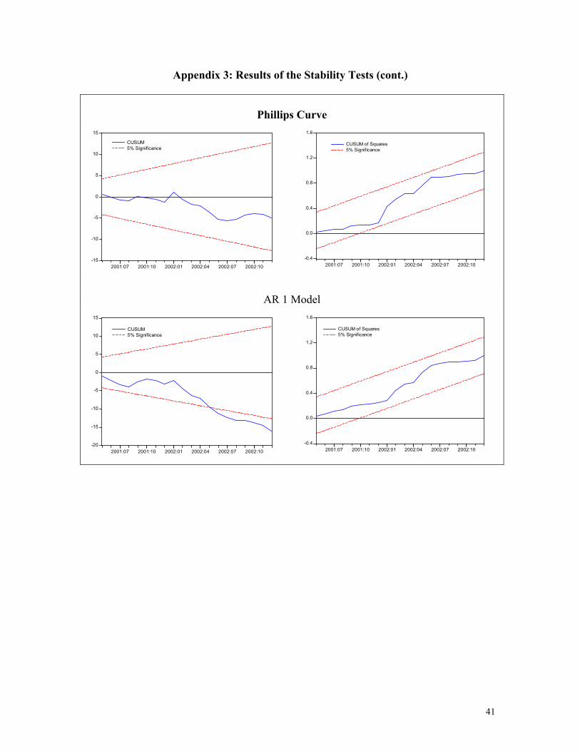
request).26 Moreover, CUSUM stability tests, presented in Appendix 3, also indicate that

the models are, by and large, stable as evidenced by the graph of the cumulative sum of

squares of recursive residuals. Next, I explore the forecasting performance of the models.

5. Comparison of the Forecasts

In an attempt to examine the out-of-sample forecasting performance of the models

considered in this paper, I estimate all the models using dynamic rolling regression

starting with 1990.01-2001.4 as the sample period, moving up one month each time to

generate a new forecast. The dynamic forecasts are true multi-step forecasts—from the

start of the forecast sample—since they employ the recursively computed forecast of the

lagged value of the dependent variable. These forecasts may be interpreted as the

forecasts for the subsequent periods that would be computed utilizing information

available at the start of the forecast sample. This exercise is conducted by using the

actual values for the explanatory variables. The selection of the forecasting period was

24In the presence of serial correlation, the coefficient estimates will still be unbiased and consistent, though they will not be the most efficient in the class of all linear unbiased estimators. This inefficiency of the estimates will manifest itself in the t-statistics generated from the coefficients, leading to dubious t-statistics. 25 It should be noted that the high RESET statistic in the case of mark-up model I indicates a problem with the chosen specification, which I did not try to solve here. 26 Since it would be preferable to base our forecasts on a model with a simple error structure, I did not attempt to correct for serial correction in the cases of the mark-up II, the Phillips curve, and mgapm2 models.

28

motivated by the adoption of a new economic program in May 2001 with a view to shed

light on the out-of-sample performance of the models under the new regime based, inter

alia, on the floating exchange rate and the new Central Bank Law.

I rely on the three most commonly used measures of predictive accuracy, namely

root mean square error (RMSE), mean absolute error (MAE), and Theil’s inequality

coefficient. The RMSE is a better performance criterion when the variable of interest

undergoes fluctuations and turning points. The RMSE penalizes models with large

prediction errors more than MAE does. If the variable displays a steady trend, MAE

might be preferred to RMSE since then one is concerned with how far above or below the

actual data line the simulation falls. Theil’s inequality coefficient ranges between 0 and

1, with 0 indicating perfect prediction.

In addition to these forecasting measures, I also employ relative absolute error

(RAE) proposed by Armstrong and Collopy (1992) as an alternative. They argue that, for

the purpose of comparing time series forecasts, the RAE is more appropriate than the

RMSE. The RAEs for a particular forecasting method are summarized across all the H

horizons on a particular series by the following expression:

(10)

,,,1

,,,1,

AF

AFCumRAE

shshrw

H

h

shshm

H

hsm

−∑

−∑=

=

=

where H, h, s, Fm,h,s, Ah,s, and rw are the number of horizons to be forecast, the horizon

being forecast, the series being forecast, the forecast from method m for horizons h of

series s, the actual value at horizon h of series s, and the random walk method,

respectively.

29

Table 7 reports the forecast errors. The results imply that the best performing

model based on out-of-sample performance is the Phillips curve model. The money gap

model using M1 definition is a close second followed by the money gap (mb) model,

mark-up model II, mark-up model I, and money gap (M2) model. The findings indicate

that all models outperform the AR1 specification.

Table 7: Out of Sample Forecasting Performance (Dynamic)a Root Mean

Squared Error Mean Absolute

Error Theil’s

Inequality Coefficient

CumRAE

Mark-up I 0.016428 0.013181 0.244261 0.713678

Mark-up II 0.016261 0.013512 0.235664 0.731572

Money Gap (mb) 0.015594 0.012741 0.215036 0.689854

Money Gap (M1) 0.015025 0.012991 0.199086 0.703381

Money Gap (M2) 0.017782 0.015300 0.232011 0.828371

Phillips Curve 0.014489 0.011544 0.215639 0.625015

AR1 0.019398 0.017409 0.240598 NAb a: Estimation period: 1990.01-2001.04; Forecasting period: 2001.05-2002.12 b: Not applicable

6. Policy Implications and Conclusion

The successful performance of a number of industrialized countries that have

adopted inflation targeting (IT) has rendered this monetary policy strategy an attractive

alternative for emerging market economies (EMs). Indeed, a number of EMs has already

instituted IT or some form of this monetary policy framework. The growing attraction of

inflation targeting among EMs as a monetary policy framework has, in turn, increased the

importance of understanding inflation dynamics and forecasting the future path of

inflation in these countries.

30

In light of the envisioned adoption of this regime in Turkey, this study considers

the case of Turkey and examines the in-sample and out-of sample performance of models

that have some theoretical foundations for the period January 1990-December 2002. To

this end, the investigation focuses on mark-up models, monetary models, the Phillips

curve, and the simple AR1 specification. The results from the in-sample estimations

suggest that mark-up models perform better than money-gap models and the Phillips

curve in explaining movements in Turkish inflation during the period under

consideration. The findings also indicate that all three models outperform the AR1

specification, which was selected as a benchmark.27

The empirical results from the out-of-sample forecasting performance for the

period May 2001-December 2002, however, turned out to be quite different. More

specifically, the findings show that the Phillips curve and money gap models have better

out-of-sample forecasting performance compared to mark-up models since the inception

of the new economic program.

There are two main policy implications emerging from the thrust of the overall

findings. First, the findings suggest that the Turkish economy has experienced a change

in the dynamics of inflation under the new regime, which included, inter alia, the

adoption of floating exchange rates and the new Central Bank Law. This, in turn, implies

that there has been a change in the relative importance of different determinants of

inflation since the introduction of the floating regime. Although the best performing

model, based on in-sample results, turned out to be the mark-up models incorporating the

exchange rate, wages, and the administered prices, the Philips curve and money gap

27 All three models, to be useful in forecasting, should at minimum perform better than this simple univariate specification.

31

models—particularly the one based on M1 measure of money-gap—outperformed the

mark-up models when out-of sample performance was considered. As a result, it can be

argued that the relative importance of output gap and monetary disequilibrium in the

inflation process in Turkey has increased under the new regime.

Second, monetary policy, by its very nature, is conducted in an environment

characterized by uncertainty and change. The uncertainty is likely to be higher in a

country like Turkey where the economy has been undergoing significant changes. Based

on estimation and forecasting results presented in this study, it can be argued that Phillips

curves augmented with the exchange rate as well as money models might provide

complementary views in the Turkish context. In light of the experiences of other

emerging market economies that adopted IT or some form of this monetary policy

framework, it is quite possible that the relative importance of other components in the

models of the inflation process is likely to increase as the volatility of the exchange rate

and the pass-through decline over time. All in all, the findings highlight the importance

of relying on multiple models of inflation in the conduct of Turkish monetary policy.

32

References

Agenor, P. and P. Montiel (1999), “Development Macroeconomics”, Princeton University Press, Princeton, New Jersey.

Altimari, S. N. (2001), “Does Money Lead Inflation in the Euro Area?”, European Central Bank Working Paper, No. 63.

Armour, J. J. Atta-Mensah, W. Engert, and S. Hendry (1996), “A Distant Early Warning Model of Inflation Based on M1 Disequilibria”, Bank of Canada Working Paper, No: 96-05.

Bahmani-Oskooee, M. I. Domaç (2003), “On the Link between Dollarization and Inflation: Evidence from Turkey", forthcoming in Comparative Economic Systems.

Bailliu, J. D. Garces, M Kruger, and M. Messmacher (2002), “Explaining and Forecasting Inflation in Emerging Markets: the Case of Mexico”, Working Paper written as part of Research Collaboration Program between the Bank of Canada and the Baco de Mexico..

Blinder, A. S. (1998), “Central Banking in Theory and Practice”, Cambridge, Mass.: MIT Press.

Boone, L., M. Juillard, D. Laxton, and P. N’Diaye (2002), “How Well Do Alternative Time-Varying Models of the NAIRU Help Policymakers Forecast Unemployment?”, Forthcoming, IMF Working Paper.

Callen, T. and Chang, D. (1999), “Modeling and Forecasting Inflation in India”, IMF Working Paper, No: WP/99/119.

CBRT, Monetary Policy Report (2002), April.

_____, Inflation Report (2000), July.

Catão, L. and M. Terrones (2001), “Fiscal Deficits and Inflation: A New Look at the Emerging Market Evidence”, IMF Working Paper, No: WP/01/74.

Coe. D.T. and C.J. McDermott. (1999), “Does the Gap Model Work in Asia?”, IMF Staff Papers, vol. 44(1), pp. 59-80.

Conesa Labastida, A. (1998), “Pass-Through del Tipo de Cambio y del Salario: Teoría y Evidencia para la Industria Manufacturera en México”, Banko de México Working Paper, No: 9803.

Engert, W. and J. Selody. (1998), “Forecasting Inflation with the M1-VECM: Part Two”, Bank of Canada Working Paper, 98-6.

Fischer, S., R. Sahay and C. Vegh. (2002), “Modern Hyper- and High Inflations”, Journal of Economic Literature, Forthcoming.

Friedman, M. (1968), “The Role of Monetary Policy”, American Economic Review, vol. 58, pp. 1-17.

Fung, B.S.C. and M. Kasumovich (1998), “Monetary Shocks in the G-6 Countries: Is There a Puzzle?”, Journal of Monetary Economics, vol. 42(3), pp. 575-92.

33

Gali, J., M. Gertler and J.D. Lopez-Salido (2001), “European Inflation Dynamics”, European Economic Review, vol. 45(7), pp. 1237-70.

Garces Díaz, D.G. (1999), “Determinación del Nivel de Precios y la Dínamica Inflacionaria en México”, Banco de México Working Paper, No: 9907.

Garcia, C. and J. Restrepo (2001), “Price Inflation and Exchange Rate Passthrough in Chile”, Banco de Chile working Paper, No: 128.

Goodfriend, M. and R. King (1997), “The New Neoclassical Synthesis”, In NBER Macroeconomics Annual 1997, ed. By B. Bernanke and J. Rotemberg. Cambridge, Mass.: MIT Press.

Goodfriend, M. (1997), “A Framework for the Analysis of Moderate Inflations”, Journal of Monetary Economics, vol. 39(1), pp. 45-66.

Gordon, R.J. (1997), “The Time-Varying NAIRU and its Implications for Economic Policy”, Journal of Economic Perspectives, vol. 11(1), pp. 11-32.

Gutierrez, E. (2003), “Inflation Performance and Constitutional Central Bank Independence: Evidence from Latin American and the Caribbean”, IMF Working Paper, No: 53.

Haan, J. and D. Zelhorst (1990), “The Impact of Government Deficits on Money Growth in Developing Countries”, Journal of International Money and Finance, vol. 9, pp. 455-69.

Hallman, J.J., Porter, R.D. and Small, D.H. (1991), “Is the Price Level Tied to the M2 Monetary Aggregate in the Long Run?”, American Economic Review, vol.81(4), pp. 841-858.

Hendry, S. (1995), “Long-Run Demand for M1”, Bank of Canada Working Paper, 95-11.

International Monetary Fund (1996), “The Rise and Fall of Inflation: Lessons from the Postwar Experience”, World Economic Outlook, October, Chapter VI. Washington, D.C.: International Monetary Fund.

_____(2001), “The Decline of Inflation in Emerging Markets: Can it be Maintained?”, World Economic Outlook, May, Chapter IV. Washington, D.C.: International Monetary Fund.

Jonsson, G. (1999), “Inflation, Money Demand, and Purchasing Power Parity in South Africa”, IMF Working Paper, No: WP/99/122.

Kasumovich, M. (1996), “Interpreting Money-Supply and Interest-Rate Shocks as Monetary-Policy Shocks”, Bank of Canada Working Paper, No: 96-8

Kibritçioğlu, A. (2001), “Causes of Inflation in Turkey: A Literature Survey with Special Reference to Theories of Inflation”, University of Illinois at Urbana-Champaign, Office of Research Working Paper, No: 01-0115

King, M. (2002), “No money, no inflation—the role of money in the economy”, Bank Of England Quarterly Bulletin, summer 2002.

Kremers, J., N.R Ericsson and J.J. Dolado (1992), “The Power of Cointegration Tests”, Oxford Bulletin of Economics and Statistics, vol. 54(3), pp. 325-348.

34

Lipsey, R. G. (1960), “The Relationship Between Unemployment and the Rate of Change of Money Rates in the U.K., 1862-1957: A Further Analysis”, Economica, vol. 27, pp. 1-32.

Longworth, D. and C. Freedman. (2000), “Models, Projections and the Conduct of Policy at the Bank of Canada”, Paper prepared for the conference “Stabilization and Monetary Policy: The International Experience,” Banco de Mexico, November 14-15.

Lougani, P. and P. Swagel (2001), “Sources of Inflation in Developing Countries”, IMF Working Paper, No: WP/01/198.

Lucas, R. (1996), “Nobel Lecture: Monetary Neutrality”, Journal of Political Economy,

vol.104.

Mohanty, M.S. and M. Klau (2001), “What Determines Inflation in Emerging Market Countries?”, BIS Papers, No. 8: Modeling Aspects of the Inflation Process and Monetary Transmission Mechanism in Emerging Market Countries.

Newey, W. and K. West (1987), “A Simple Positive Definite, Heteroskedasticity and Autocorrelation Consistent Covariance Matrix”, Econometrica, vol 55, pp. 703-708.

Özcan, K. M., Berument, M. H., and Neyaptı, B. (2001), “Dynamics of Inflation and Inflation Inertia in Turkey”, unpublished manuscript Bilkent University.

Paşaoğulları, M and T. Yurttutan (2002), “Alternative Output Gap Measures: Review of Statistical Methodologies and Applications to Turkish Data”, Mimeo, the Central Bank of the Republic of Turkey.

Perez-López, A. (1996), “Un Estudio Econométrico sobre la Inflacíon en México” Banco de México Working Paper, No: 9604.

Perron, P. (1989), “The Great Crash, the Oil Price Shock, and the Unit Root Hypothesis”, Econometrica, vol. 57, pp. 1361-401.

Pesaran, M.H. and Shin, Y. (1997), “An Autoregressive Distributed Lag Modeling Approach to Cointegration Analysis, in S. Strass, A. Holly and P. Diamond (eds.), Centennial Volume of Rangar Frisch, Econometric Society”, Cambridge University Press, Cambridge.

Pesaran, M.H., Shin, Y. and Smith, R.J. (1996), “Testing for the Existence of a Long Run Relationship”, Department of Applied Economics Working Paper, No. 9622, University of Cambridge.

Phillips, A.W. (1958), “The Relationship Between Unemployment and the Rate of Change of Money Wages in the United Kingdom, 1861-1957”, Economica, vol 25, pp. 283-299.

Phillips, A. and B. Hansen (1990), “Statistical Inference in Instrumental Variable Regression with I(1) Processes”, Review of Economic Studies, vol 57, pp. 99-125.

35

Sakallıoglu, U. C. and Yeldan, A. E. (1999), “Dynamics of Macroeconomic Disequilibrium and Inflation in Turkey: The State, Politics, and the Markets Under a Globalized Developing Economy”, Bilkent University Department of Economics Working Paper, No: 99-10.

Santaella, J.A. (2001), “El Traspaso inflacionario del Tipo de Cambio, la Paridad del Poder de Compra y Anexas: La Experiencia Mexicana”, In La Inflación en México, Gaceta de Economía, ITAM, forthcoming.

Simone, F. (2000), “Forecasting Inflation in Chile Using State-Space and Regime-Switching Models”, IMF Working Paper, No: WP/00/162.

Springer, P. and M. Kfoury (2002), “A Simple Model for Inflation Targeting in Brazil”, Brazilian Journal of Applied Economics, vol, 6(1), pp. 31-48.

Stock, J.H., and M.W. Watson (1999), “Forecasting Inflation”, Journal of Monetary Economics, vol. 44, pp. 293-335.

36

Appendix 1: Data Definition and Sources

Domestic price level (P): is defined as the Turkish consumer price index, source a.

Exchange rate (E): is the spot exchange rate defined as the number of Turkish Lira per

US dollar, source b.

Administered prices (ap): includes the prices controlled by the Government, source a.

Foreign price level (P*): is the US consumer price index, source c.

Wages (W): wages in manufacturing industry, source a.

Monetary base (mb): Currency Issued + Required Reserves (in TL) + Free Deposits,

source b.

M1: Currency in circulation + demand deposits, source b.

M2: M1 + time deposits, source b.

All data are monthly covering January 1990- December 2002 and are obtained

from the following sources: (a) State Institute of Statistics; (b) The Central Bank of

Turkey; (c) IMF’s International Financial Statistics.

37

Appendix 2: Figures of Series

Output Gap CPI Inflation

-12

-8

-4

0

4

8

90 91 92 93 94 95 96 97 98 99 00 01 02-4

0

4

8

12

16

20

24

90 91 92 93 94 95 96 97 98 99 00 01 02

Nominal exchange ratea Wagesa

-10

0

10

20

30

40

50

90 91 92 93 94 95 96 97 98 99 00 01 02-8

-4

0

4

8

12

16

20

24

90 91 92 93 94 95 96 97 98 99 00 01 02

Administered Pricesa Money-gap (mb)

0

10

20

30

40

50

60

90 91 92 93 94 95 96 97 98 99 00 01 02-.20

-.15

-.10

-.05

.00

.05

.10

.15

.20

90 91 92 93 94 95 96 97 98 99 00 01 02

a: Rate of change

38

Appendix 3: Results of the Stability Tests

Mark-up Model I

-12

-8

-4

0

4

8

12

2001:07 2001:10 2002:01 2002:04 2002:07

CUSUM5% Significance

-0.4

0.0

0.4

0.8

1.2

1.6

2001:07 2001:10 2002:01 2002:04 2002:07

CUSUM of Squares5% Significance

Mark-up Model II

-12

-8

-4

0

4

8

12

2001:07 2001:10 2002:01 2002:04 2002:07

CUSUM5% Significance

-0.4

0.0

0.4

0.8

1.2

1.6

2001:07 2001:10 2002:01 2002:04 2002:07

CUSUM of Squares5% Significance

39

Appendix 3: Results of the Stability Tests (cont.)

Money Gap Model (mb)

-15

-10

-5

0

5

10

15

2001:07 2001:10 2002:01 2002:04 2002:07 2002:10

CUSUM5% Significance

-0.4

0.0

0.4

0.8

1.2

1.6

2001:07 2001:10 2002:01 2002:04 2002:07 2002:10

CUSUM of Squares5% Significance

Money Gap Model (M1)

-20

-15

-10

-5

0

5

10

15

2001:07 2001:10 2002:01 2002:04 2002:07 2002:10

CUSUM5% Significance

-0.4

0.0

0.4

0.8

1.2

1.6

2001:07 2001:10 2002:01 2002:04 2002:07 2002:10

CUSUM of Squares5% Significance

Money Gap Model (M2)

-20

-15

-10

-5

0

5

10

15

2001:07 2001:10 2002:01 2002:04 2002:07 2002:10

CUSUM5% Significance

-0.4

0.0

0.4

0.8

1.2

1.6

2001:07 2001:10 2002:01 2002:04 2002:07 2002:10

CUSUM of Squares5% Significance

40

Appendix 3: Results of the Stability Tests (cont.)

Phillips Curve

-15

-10

-5

0

5

10

15

2001:07 2001:10 2002:01 2002:04 2002:07 2002:10

CUSUM5% Significance

-0.4

0.0

0.4

0.8

1.2

1.6

2001:07 2001:10 2002:01 2002:04 2002:07 2002:10

CUSUM of Squares5% Significance

AR 1 Model

-20

-15

-10

-5

0

5

10

15

2001:07 2001:10 2002:01 2002:04 2002:07 2002:10

CUSUM5% Significance

-0.4

0.0

0.4

0.8

1.2

1.6

2001:07 2001:10 2002:01 2002:04 2002:07 2002:10

CUSUM of Squares5% Significance

41