expertrna: a new framework for rna structure prediction

ExpertRNA: A new framework for RNA structure prediction

Menghan Liu, Giulia Pedrielli

Arizona State University, School of Computing Informatics and Decision Systems Engineering

Erik Poppleton, Petr Sulc

Arizona State University, School of Molecular Sciences and Center for Molecular Design and Biomimetics.

Dimitri P. Bertsekas

Arizona State University, School of Computing Informatics and Decision Systems Engineering

Massachussets Institute of Technology, Electrical Engineering.

January 17, 2021

Abstract

Ribonucleic acid (RNA) is a fundamental biological molecule that is essential to all living organisms,

performing a versatile array of cellular tasks. The function of many RNA molecules is strongly related to

the structure it adopts. As a result, great effort is being dedicated to the design of efficient algorithms

that solve the “folding problem”: given a sequence of nucleotides, return a probable list of base pairs,

referred to as the secondary structure prediction. Early algorithms have largely relied on finding

the structure with minimum free energy. However, the predictions rely on effective simplified free

energy models that may not correctly identify the correct structure as the one with the lowest free

energy. In light of this, new, data-driven approaches that not only consider free energy, but also use

machine learning techniques to learn motifs have also been investigated, and have recently been shown

to outperform free energy based algorithms on several experimental data sets.

In this work, we introduce the new ExpertRNA algorithm that provides a modular framework which

can easily incorporate an arbitrary number of rewards (free energy or non-parametric/data driven)

and secondary structure prediction algorithms. We argue that this capability of ExpertRNA has the

potential to balance out different strengths and weaknesses of state-of-the-art folding tools. We test

the ExpertRNA on several RNA sequence-structure data sets, and we compare the performance of

ExpertRNA against a state-of-the-art folding algorithm. We find that ExpertRNA produces, on average,

more accurate predictions than the structure prediction algorithm used, thus validating the promise of

the approach.

Keywords: RNA folding, secondary structure prediction, rollout

1 Introduction

Ribonucleic acid (RNA) is a fundamental biological macromolecule that is essential to all living organisms,

performing a versatile array of cellular tasks including information transfer, enzymatic function, sensing,

regulation, and structural function (Elliott and Ladomery, 2017). RNA has recently emerged as a promising

drug target, with new therapeutic approaches aiming to develop drugs that target RNA rather than

1

(which was not certified by peer review) is the author/funder. All rights reserved. No reuse allowed without permission. The copyright holder for this preprintthis version posted January 19, 2021. ; https://doi.org/10.1101/2021.01.18.427087doi: bioRxiv preprint

https://doi.org/10.1101/2021.01.18.427087

proteins. Moreover, designed RNA molecules are used in rapidly growing fields of synthetic biology and

RNA nanotechnology, with applications to diagnostics, immunotherapy, drug delivery and realization of

logical operations inside cells (Green et al., 2014; Geary et al., 2014; Hochrein et al., 2013; Han et al.,

2017; Guo, 2010; Qi et al., 2020). In particular, such functionalities are enabled by the 3D structure the

RNA molecules fold into. Each RNA molecule is made up of individual units, nucleotides (bases), that are

of four types, A, U, G and C. A molecule is then uniquely defined by its sequence and structure. The

sequence is a string with the A, U, C, G bases reported in the order they appear. RNA sequences range in

length from tens (tRNAs, siRNAs) to tens of thousands (e.g. viral genomes and long non-coding RNAs) of

nucleotides. The structure, i.e., the way nucleotides are interacting in space, can be represented through

an incidence matrix (each cell is (1, 0) if the nucleotides are linked or not, respectively) or dot-bracket

notation (Sect. 3). In particular, the primary structural elements of RNA molecules are base pairs, i.e.,

bonds between bases that are not contiguous. The most common types of base pairings, referred to as the

“canonical base pairs”, are (i) the Watson-Crick base pairs, where a nucleotide of type A pairs with U, G

pairs with C, and (ii) the wobble base pair, where a nucleotide of type G pairs with U. Given a sequence,

a set of canonical base pairs defines the secondary structure, which is often used as a first approximation

of the RNA structure. The tertiary structure is a more accurate representation that also considers weaker

interactions compared to the base pairing. Together, these interactions determine the three-dimensional

relative orientation of nucleotides.

Given the impact of structure on RNA functionality, the accurate computational prediction of the

secondary and tertiary structure of RNA is an ongoing area of great interest in the computational biology

community (Calonaci et al., 2020; Cruz et al., 2012; Wayment-Steele et al., 2020).

Secondary Structure Prediction. Most tools for secondary structure prediction (Reuter and Mathews,

2010; Hofacker, 2003; Zadeh et al., 2011; Zuker and Stiegler, 1981) attempt to identify the structure that

minimizes the free energy (FE) associated with the RNA molecule upon pairing a subset of the nucleotides,

i.e., the energy released by folding a completely unfolded RNA sequence. The underlying assumption

is that the structure with the lowest free energy is also the most likely structure the RNA will adopt.

Equivalently, this family of approaches relies on the basic idea that the lower the FE the more stable the

RNA structure will be. A first challenge for this family of approaches is that it is not possible to exactly

calculate the free energy due to the (i) incomplete understanding of the RNA molecular interactions, and

(ii) the impractical computational cost of detailed kinetic simulation tools. As a result, several approximate

models have been proposed in the literature (Mathews et al., 1999; Xia et al., 1998; Andronescu et al., 2007,

2010) to estimate the free energy associated with a given secondary structure. Most of the computational

savings are a result of ignoring tertiary interactions. A second, and possibly deeper, challenge is that this

model assumes that an “optimal” structure is one that pairs nucleotides in a way that minimizes the free

energy (MFE). However, RNA is known to fold cotranscriptionally (Angela et al., 2018), equivalently,

RNA molecules might adopt a kinetically-preferred structure different from the global free energy minima.

In light of these challenges, alternative approaches to structure prediction have been proposed. Stochas-

tic kinetic folding algorithms (Isambert and Siggia, 2000; Sun et al., 2018) approximate the folding kinetics

of RNA molecules as they are transcribed. Data driven approaches have also started to become popular that

use machine learning to evaluate structures rather than FE or kinetic models. These include ContraFold,

DMfold, and structure prediction with neural networks (Do et al., 2006; Wang et al., 2019; Calonaci

2


https://doi.org/10.1101/2021.01.18.427087

et al., 2020). Furthermore, in the attempt to achieve advantages of model or data driven approaches,

methods have been proposed that attempt to aggregate multiple information sources to get more accurate

secondary structure prediction. Within the data driven category, some examples of information sources are

the experimentally determined SHAPE data (Lucks et al., 2011; Low and Weeks, 2010), and evolutionary

covariation information (Calonaci et al., 2020). On the model driven side, statistical ensemble approaches

are used to boost the solutions obtained by the different FE driven folding algorithms. To the knowledge

of the authors, ensemble methods allow to mix solutions from different algorithms only upon completion,

i.e., they do not enable interaction among the algorithms while they are running (Aghaeepour and Hoos,

2013). A recent survey on a set of secondary structure prediction tools has reported mixed results, with

data-driven approaches generally outperforming the ones based on nearest-neighbor free energy models,

and with model-based ensemble approaches showing competitive results (Wayment-Steele et al., 2020).

Tertiary Structure Prediction. Concerning the tertiary structure prediction problem, fewer approaches

can be found in the literature (Seetin and Mathews, 2011; Westhof and Auffinger, 2006; Tan and Chen,

2010; Miao et al., 2017; Watkins et al., 2020). In fact, the prediction of tertiary structures is particularly

challenging, and most prediction methods only work for short RNA sequences (tens of nucleotides). Data

driven approaches have attracted attention also for the tertiary structure prediction. However, their

accuracy remains limited due to the small number of 3D RNA structure data sets available for model

training and verification.

Stemming from the observation that several folding algorithms have been proposed in the literature for

secondary and, even if fewer, for tertiary structure prediction, without any approach dominating the

other, we propose the idea to build a framework that can exploit several folding tools and criteria to

evaluate the quality of a folded sequence, during the algorithm execution. The aim of our approach is to

achieve a better RNA structure prediction quality. The result of our work is ExpertRNA, which allows to

combine multiple secondary structure prediction algorithms (equivalently referred to as folding algorithms

or folders), whose predictions are sequentially evaluated by a set of experts that score the quality of the

predicted structures based upon their own scoring criteria. ExpertRNA is based on rollout (Bertsekas,

2020), an approximate dynamic programming technique, which, given an algorithm called base policy

(or base heuristic), generates an improved algorithm, called rollout policy, as evaluated by one or more

“experts”. Rollout also allows the use of multiple base policies and it provably improves (relative to the

expert score) on the performance of each of them.

We argue that ExpertRNA has the potential to exploit the strengths of the folding tool being used by the

algorithm itself as base heuristic, by improving on the solution by using several experts. In this manuscript,

we focus on secondary structure prediction, and we use RNAfold (a free energy based folder (Lorenz

et al., 2011)) as the base heuristic (Sect. 2), and, as expert, we use two different implementations of the

state-of-the-art tool ENTRNA (a classifier that evaluates the quality of a sequence-structure pair (Su et al.,

2019)) to judge sequence-structure pairs generated by a folding algorithm (Sect. 2). We test ExpertRNA

against two popular RNA sequence-structure data sets: Rfam (Burge et al., 2013), and the Mathews

data set (Ward et al., 2017). We compare the performance of ExpertRNA against RNAfold, when used

in isolation. We find that, in the sequences taken from Rfam, ExpertRNA produces, on average, more

accurate predictions of secondary structure, and performs, on average, the same on the Mathews data set.

3


https://doi.org/10.1101/2021.01.18.427087

2 Relevant Literature

With respect to our work, we distinguish two main branches of research within the rich literature in RNA

secondary structure prediction: (i) model driven, and (ii) data driven approaches. As mentioned in Sect. 1,

most of model driven approaches use the Free Energy (FE) as reference reward function to be minimized.

Algorithms differ in the model used to approximate the FE and the mechanisms to explore the space of

possible structures, in the attempt to find the minimum FE (MFE). Data driven approaches use machine

learning techniques to evaluate the quality of the structure as a replacement, or, possibly, in addition to

FE. In this case, FE is interpreted as a feature instead of the reward.

2.1 Model driven folding

The most common approach for evaluating RNA structures is its free energy, which can be thought of as

the energy released by folding a completely unfolded RNA sequence. It can also be interpreted as the

amount of energy that must be added in order to unfold a folded molecule. As a result, a sequence will

be most likely found in a minimum free energy structure. No closed form is available for the exact free

energy calculation, and algorithms differ in the way they approximate such computation, and the way

they search in the space of secondary structures attempting to find the one(s) with associated minimum

(approximated) free energy (Lorenz et al., 2011). An example of minimum free energy approximation

relies on the nearest-neighbor model (NN-M) (Xia et al., 1998). The NN-M relies on the assumption that

each base pair contributes to the overall free energy independently from one another, and a base pair is

only influenced by the immediately adjacent base pairs. As a result of these assumptions, the total free

energy is the sum of all the base pair free energies, along with additional terms that account for the free

energy contribution of motifs such as hairpin loops, internal loops, and bulges and junctions (Mathews

et al., 1999) (Fig. 1). Using the free energy minimization criteria, any predicted “optimal” secondary

structure for an RNA molecule depends on the model of folding and the specific folding energies used to

calculate that structure. A consequence of this is that different optimal structures may be obtained if the

folding energies are changed even slightly.

An example of algorithm relying on FE is RNAfold, a de-facto standard tool for RNA secondary

structure prediction. The RNAfold software (Lorenz et al., 2011) makes use of the NN-M to sequentially

assign nucleotides to the partially folded sequence. Importantly, RNAfold allows constrained folding, i.e.,

users can input information concerning pairings between nucleotides that they wish to fix and/or just

constraining nucleotides to be paired without defining the nucleotide to pair it with. This second type of

constraint is not generally implementable by folding packages and led us to choose RNAfold as the base

heuristic for this first version of ExpertRNA. Further examples of model based RNA folding approaches are

stochastic kinetic folding algorithms. Rather than using dynamic programming, base pairings are randomly

sampled biasing towards bonds with high energy. Energy is estimated using kinetic models, and, for

computational efficiency, the kinetic model is called only to evaluate the partially folded structure (Isambert

and Siggia, 2000; Sun et al., 2018; Zadeh et al., 2011). Another approach is AveRNA, an ensemble-based

prediction method for RNA secondary structure (Aghaeepour and Hoos, 2013). AveRNA combines a set

of existing MFE-based secondary structure prediction procedures into an ensemble-based method aiming

to achieve higher prediction accuracy. The underlying algorithms use different models for free energy.

4


https://doi.org/10.1101/2021.01.18.427087

These models, first presented in (Andronescu et al., 2007, 2010), use the constraint generation method to

sequentially produce constraints that enforce known structures to have energies lower than other structures

for the same molecule. Such method has resulted in several FE approximation variants.

It is important to, again, highlight that one of the main drawbacks of model driven methods is that

energy models are approximations of the not fully known complex physical interactions and folding

conditions that determine the folded structure of the molecule in natural or laboratory settings. Because

of uncertainties in the folding model and the folding energies, the “true” folding may not be the “optimal”

folding determined by the algorithm. In fact, several and sub-optimal structures may exist within a few

percent of the minimum energy.

2.2 Data-driven folding

Approaches utilizing statistical learning have recently received increasing attention. Different folding

algorithms may use different statistical methods and different features to generate base pairing decisions.

The CONTRAfold algorithm falls into this category of approaches (Do et al., 2006). CONTRAfold

applies stochastic context-free grammars (SCFGs) for representing RNA structures as random objects

that are modified within a fully-automated statistical learning procedure that sequentially biases the

sampling distribution responsible for the making and breaking of base pairs within the sequentially formed

RNA structure. In particular, CONTRAfold sequentially forms and brakes base pairs updating the

probability associated to the several bonding alternatives, which is formulated using conditional log-linear

models (CLLMs). The hyperparameters of the CLLMs are estimated using several features of RNA

sequence-structure pairs. The model determines the likelihood of a base pairing (or a set of pairings)

to be selected by the algorithm (Do et al., 2006). The algorithm CycleFold (Sloma and Mathews, 2017)

differs from ContraFold because it uses sets of RNA bases as building blocks for the search, instead of the

individual nucleotides. Each of these sets has a detailed energetic characterization, thus improving the

accuracy of the energy prediction patterns. The building blocks are subsequently folded in a way similar

to other data-driven approaches (Dieckmann et al., 1996). LearnToFold (Chowdhury et al., 2019) uses

an approximate folding tool (LinearFold) as inference engine for search, and a structured support vector

machine (sSVM) to bias the sampling towards more favorable pairings. SPOT-RNA (Singh et al., 2019)

uses deep contextual learning for base pair prediction and it is one of the few to include tertiary interactions,

even if approximated. Deep and transfer learning (Hanson et al., 2020) are trained in order to calculate

the likelihood of each nucleotide to be paired with any other nucleotide in a sequence. ENTRNA (Su

et al., 2019) is a supervised learning algorithm that uses a support vector machine (SVM) to produce

an evaluation of the quality of a RNA secondary structure. In particular, ENTRNA receives as input a

sequence-structure pair and it returns a measure of the likelihood that such a pair folds, and it is stable.

Such likelihood measure is defined by the authors as foldability. The higher the foldability, the more

likely the sequence-structure pair is to exist and be stable. Alternatively, the more likely that sequence

is to fold into that structure. ENTRNA, as any data-driven approach, needs to be trained by examples

of existing sequence-structure pairs, each associated with a set of features (sequence-segment entropy

-SSE-, free energy, relative number of nucleotides of type G and C, relative number of paired nucleotides).

In particular, the SSE metric was proposed in (Su et al., 2019) to give a measure of diversity of the

nucleotides segments within the RNA sequence. However, to be trained, ENTRNA also requires failed

5


https://doi.org/10.1101/2021.01.18.427087

examples (i.e., sequence-structure pairs that cannot fold in a stable manner). This is a challenge due to the

unavailability of “failed” experiments, which the authors tackle by using the Positive-Unlabeled learning

method to fill in the failed examples (Li et al., 2009). Nevertheless, this remains a source of inaccuracy for

the approach. Similar to ENTRNA, RNAStructure (Reuter and Mathews, 2010) uses both data driven

features and free energy models to evaluate sequence-structure pairs. RNAstructure, first, contained a

method to predict the lowest free energy structure, it was subsequently expanded to include bimolecular

folding and hybridization thermodynamics, and stochastic sampling of structures. It provides methods for

constraining structures based on empirical characteristics of similar sequences. Finally, recent extensions

calculate partition functions for secondary structures common to two sequences and can perform stochastic

sampling of common structures.

2.3 Contributions

The contribution of this paper is both algorithmic and applied: (i) we extend the rollout approach to

be used with multiple heuristics and multiple experts, while controlling the number of branches being

active at each iteration of the algorithm, thus allowing to control the computational expense. We allow

the different experts to interact which leads to better solutions than allowing experts to only judge the

branches dedicated to them (Bertsekas, 2020); (ii) we exploit this algorithmic capability to maintain

multiple parallel rollout branches allowing the several experts and, potentially, folding algorithms, to

maintain multiple solutions. To our knowledge, unlike all the previously published algorithms, ExpertRNA

is the only approach allowing the different folding algorithms to interact while the structure is being folded.

We believe that this capability is the key to overcome the different challenges from the several secondary

structure prediction approaches (model and data-driven).

3 Proposed Approach

The main idea underlying ExpertRNA is to formulate secondary structure prediction (folding) as a

sequential assignment problem. Based on the description in Sect. 2, we assume a sequence of nucleotides

is given as input together with a set of physical constraints that define possible nucleotide-to-nucleotide

interactions (base pairing) that can be translated into feasible actions. It is important to formalize the

way we model RNA sequences and the related structures before introducing actions and constraints.

Specifically, our work makes use of the dot-bracket notation to represent RNA structures (Antczak

et al., 2018). According to this formalism, each nucleotide is represented by a letter, symbolizing the type

of base (A, C, G, U) and a “dot” (.), if the nucleotide is unpaired, i.e., it does not establish a bond with

any other nucleotide in the sequence, or a “bracket” otherwise. If a nucleotide pairs with another, it can

either be the origin of the pairing, in which case we represent it using an open bracket “(”, or the sink, in

which case we use a close bracket “)” (Fig. 1). Fig. 1 shows an example of an RNA sequence-structure

(Fig. 1a), and the corresponding dot bracket notation (Fig. 1b). In the following, we define the main

components of ExpertRNA.

6


https://doi.org/10.1101/2021.01.18.427087

5’ 3’

5’ 3’

Figure 1: Example of an RNA secondary structure representation, with the highlighted structural motifs:a) 2D planar structure representation; b) Dot-bracket notation. This notation only represents the basepairing and does not provide the type of nucleotide.

3.1 State and action modeling in ExpertRNA

As previously mentioned, ExpertRNA sequentially attaches bases to a partially formed structure deciding

whether to pair a base (open or closed bracket) or not. Given the same sequence, a different dot-bracket

assignment will result in a different structure.

More specifically, when we select the next element from the input sequence x ∈ {A,U,C,G}, we will

connect it to the rest of the structure by means of 3 alternative actions (represented as the top, bottom,

and right arcs from each node in Fig. 2). The right arc, used in isolation, corresponds to a dot (“.”) in

the dot bracket notation, and establishes a sequential link between bases (i.e., no base pair), while the

up/down (open/closed) arcs establish a base pair type of connection, thus corresponding to a bracket. The

number of links that can be activated at iteration k is a function of the partial structure formed by the k

nucleotides already assigned, as well as the remaining N − k nucleotides in the sequence that have not

been assigned yet. Fig. 2 reports an illustrative example of the sequential folding of the RNA molecule.

(a) Example of sequential assignment. At each iteration k, thestate is represented by the assigned nucleotides and the corre-sponding bonds (i.e., sequential or base pair type of connection).

(b) [Corresponding set ofcontrols

Figure 2: Example of assignment

We start selecting a nucleotide (A in the example in Fig. 2a) and we activate the right link, corresponding

to a “.”. At the second iteration, we select C, the next nucleotide in the sequence, and we activate the

downward link (open bracket “(”)), and the right link, thus electing C as part of a base pair. Note that, at

this point, the sink of the base pair is not established, but we have only decided that C will be part of

a base pair, as origin. This means that, further in the path generation, we will need to elect one of the

candidates to be paired with C. The third-to-fifth actions are identical and they result in three C-type

bases with the right link activated, corresponding to three dots (“.”). At this point, we select G as the

7


https://doi.org/10.1101/2021.01.18.427087

next base with the upward link active (closed bracket “(”)), thus electing G as base pair, and we connect

it to the, only feasible origin C.

Actions Generalizing the example in Fig. 2, the possible actions that we can implement, at each iteration,

are to sequence, open base pair and close base pair, with the associated dot-bracket notation “.”, “(”, “)”,

respectively. ExpertRNA proceeds to form a structure starting from from the unpaired 5’ extreme (the

“first” nucleotide in the sequence, Fig. 1), and completed once all the elements are assigned, i.e., the 3’

extreme of the sequence has been reached (the “last” nucleotide in the sequence, Fig. 1). Also, we assume

that bases assigned and links activated at iteration h cannot be changed at any iteration k > h. Let us

consider a sequence of actions {u1, . . . , uk} corresponding to the assignment of the first k nucleotides out

of a N -nucleotides long sequence, with k < N . Equivalently, {u1, . . . , uk} is a partial assignment. Our

objective is to sequentially perform sequence-structure assignments using a set of well defined elementary

actions. A structure is complete when k = N .

Feasibility Determination As previously mentioned, at each iteration of the algorithm, we can either

execute a (i) “null” action (sequencing), or (ii) base pairing the nucleotide. When evaluating the feasibility

of an action the following items need to be considered:

• nucleotides of type A can only form a base pair with U;

• nucleotides of type G can only form a base pair with C or U;

• nucleotides of type U only form a base pair with A or G;

• nucleotides of type C only form a base pair with G;

• to be paired i and j need to satisfy |i− j| ≥ 4, where i and j are the location indexes of the two

nucleotides.

Hence, at each iteration, the set of feasible actions depends on the partial sequence u1, . . . , uk generated

by the procedure up to iteration k, as well as the nucleotides k + 1, . . . , N that remain to be sequenced.

3.2 ExpertRNA Algorithm

The proposed ExpertRNA tackles the problem of RNA secondary structure prediction as a sequential

assignment of (known) nucleotides.

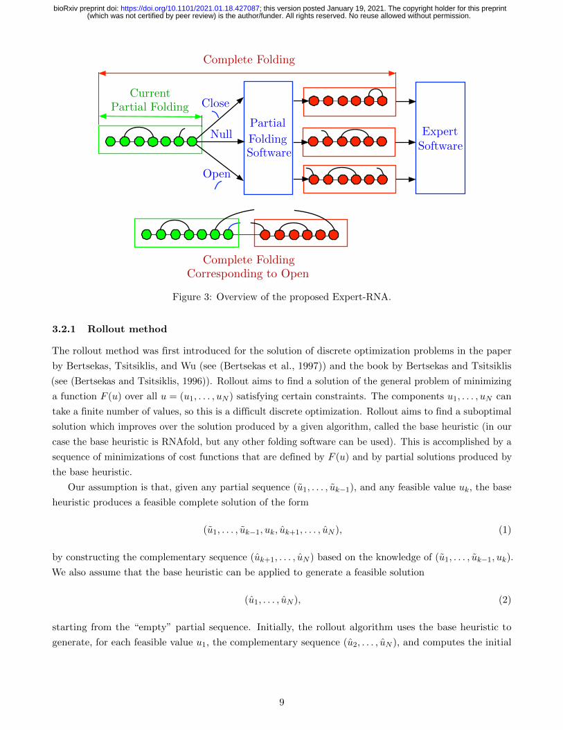
Fig. 3 shows the structure of our ExpertRNA approach with its two main algorithmic components:

(i) the partial folding; and the (ii) expert software. The algorithm sequentially adds elements to the

incomplete structure (“current partial folding” in Fig. 3), which we initialize to be the empty set. The

first nucleotide is chosen as the first element of the input sequence provided by the user. At each step, the

subsequent nucleotide is selected, and we can choose whether to simply sequence it to the last assigned

nucleotide (“Null” action in Fig. 3) or pair it with any nucleotide in the existing structure (“Close” in

Fig. 3), or pair it with an element still to be assigned (“Open” in Fig. 3). The definition of these actions

is motivated by the physical laws that govern molecular bonding (as previously specified in feasibility

determination).

8


https://doi.org/10.1101/2021.01.18.427087

Partial Folding Software Critic Software Facilities xij i j zj = 0 or 1 Sample Space Event {a ≤ X ≤ b}a b x PDF fX(x) δ x x + δ

Clients Facilities xij i j zj = 0 or 1

minuk,µk+1,...,µk+ℓ−1

E

{gk(xk, uk, wk) +

k+ℓ−1∑

i=k+1

gi

(xi, µi(xi), wi

)+ Jk+ℓ(xk+ℓ)

}

bk Belief States bk+1 bk+2 Policy µ m Steps

Truncated Rollout Policy µ m Steps Φr∗λ

B(b, u, z) h(u) Artificial Terminal to Terminal Cost gN(xN ) ik bk ik+1 bk+1 ik+2 uk uk+1 uk+2

Original System Observer Controller Belief Estimator zk+1 zk+2 with Cost gN (xN )

µ COMPOSITE SYSTEM SIMULATOR FOR POMDP

(a) (b) Category c(x, r) c∗(x) System PID Controller yk y ek = yk − y + − τ Object x hc(x, r) p(c | x)

uk = rpek + rizk + rddk ξij(u) pij(u)

Aggregate States j ∈ S f(u) u u1 = 0 u2 uq uq−1 . . . b = 0 ik b∗ b∗ = Optimized b Transition Cost

Policy Improvement by Rollout Policy Space Approximation of Rollout Policy at state i

One-step Lookahead with J(j) =∑

y∈A φjyr∗y bk Control uk = µk(bk)

p(z; r) 0 z r r + ϵ1 r + ϵ2 r + ϵm r − ϵ1 r − ϵ2 r − ϵm · · · p1 p2 pm

... (e.g., a NN) Data (xs, cs)

V Corrected V Solution of the Aggregate Problem Transition Cost Transition Cost J∗

Start End Plus Terminal Cost Approximation S1 S2 S3 Sℓ Sm−1 Sm

Disaggregation Probabilities dxi dxi = 0 for i /∈ Ix Base Heuristic Truncated Rollout

Aggregation Probabilities φjy φjy = 1 for j ∈ Iy Selective Depth Rollout Policy µ

Maxu State xk Policy µk(xk, rk) h(u, xk, rk) h(c, x, r) hu(xk, rk) Randomized Policy Idealized

Generate “Improved” Policy µ by µ(i) ∈ arg minu∈U(i) Qµ(i, u, r)

State i y(i) Ay(i) + b φ1(i, v) φm(i, v) φ2(i, v) J(i, v) = r′φ(i, v)

1




E

{gk(xk, uk, wk) +

k+ℓ−1∑

i=k+1

gi

(xi, µi(xi), wi

)+ Jk+ℓ(xk+ℓ)

}





















1




E

{gk(xk, uk, wk) +

k+ℓ−1∑

i=k+1

gi

(xi, µi(xi), wi

)+ Jk+ℓ(xk+ℓ)

}





















1




E

{gk(xk, uk, wk) +

k+ℓ−1∑

i=k+1

gi

(xi, µi(xi), wi

)+ Jk+ℓ(xk+ℓ)

}





















1

Partial Folding Software Critic Software Complete Folding Current Partial Folding

Clients Facilities xij i j zj = 0 or 1 Open Close Null


E

{gk(xk, uk, wk) +

k+ℓ−1∑

i=k+1

gi

(xi, µi(xi), wi

)+ Jk+ℓ(xk+ℓ)

}





















1




E

{gk(xk, uk, wk) +

k+ℓ−1∑

i=k+1

gi

(xi, µi(xi), wi

)+ Jk+ℓ(xk+ℓ)

}





















1




E

{gk(xk, uk, wk) +

k+ℓ−1∑

i=k+1

gi

(xi, µi(xi), wi

)+ Jk+ℓ(xk+ℓ)

}





















1

Termination State Constraint Set X X = X X Multiagent

Current Partial Folding


Approximation of E{·}: Approximate minimization:

minu∈U(x)

n∑

y=1

pxy(u)(g(x, u, y) + αJ(y)

)

x1k, u1

k u2k x2

k dk τ

Q-factor approximation

u1 u1 10 11 12 R(yk+1) Tk(yk, uk) =(yk, uk, R(yk+1)

)∈ C

x0 u∗0 x∗

1 u∗1 x∗

2 u∗2 x∗

3 u1 x2 u2 x3

x0 u∗0 x∗

1 u∗1 x∗

2 u∗2 x∗

3 u0 x1 u1 x1

High Cost Transition Chosen by Heuristic at x∗1 Rollout Choice

Capacity=1 Optimal Solution 2.4.2, 2.4.3 2.4.5

Permanent Trajectory Tentative Trajectory Optimal Trajectory Cho-sen by Base Heuristic at x0 Initial

Base Policy Rollout Policy Approximation in Value Space n n − 1n − 2

One-Step or Multistep Lookahead for stages Possible Terminal Cost

Approximation in Policy Space Heuristic Cost Approximation for

for Stages Beyond Truncation yk Feature States yk+1 Cost gk(xk, uk)

Approximate Q-Factor Q(x, u) At x Approximation J

minu∈U(x)

Ew

{g(x, u, w) + αJ

(f(x, u, w)

)}

Truncated Rollout Policy µ m Steps

Approximate Q-Factor Q(x, u) At x

Cost Data Policy Data System: xk+1 = 2xk + uk Control constraint:|uk| ≤ 1

Cost per stage: x2k + u2

k

{X0, X1, . . . , XN} must be reachable Largest reachable tube

x0 Control uk (ℓ − 1)-Stages Base Heuristic Minimization

Target Tube 0 k Sample Q-Factors (ℓ − 1)-Stages State xk+ℓ = 0

1





minu∈U(x)

n∑

y=1


)

x1k, u1

k u2k x2

k dk τ



)∈ C

x0 u∗0 x∗

1 u∗1 x∗

2 u∗2 x∗

3 u1 x2 u2 x3

x0 u∗0 x∗

1 u∗1 x∗

2 u∗2 x∗

3 u0 x1 u1 x1









minu∈U(x)

Ew

{g(x, u, w) + αJ

(f(x, u, w)

)}





k



Target Tube 0 k Sample Q-Factors (ℓ − 1)-Stages State xk+ℓ = 0

1




Complete Folding Corresponding to Open


minu∈U(x)

n∑

y=1


)

x1k, u1

k u2k x2

k dk τ



)∈ C

x0 u∗0 x∗

1 u∗1 x∗

2 u∗2 x∗

3 u1 x2 u2 x3

x0 u∗0 x∗

1 u∗1 x∗

2 u∗2 x∗

3 u0 x1 u1 x1









minu∈U(x)

Ew

{g(x, u, w) + αJ

(f(x, u, w)

)}





k



1






minu∈U(x)

n∑

y=1


)

x1k, u1

k u2k x2

k dk τ



)∈ C

x0 u∗0 x∗

1 u∗1 x∗

2 u∗2 x∗

3 u1 x2 u2 x3

x0 u∗0 x∗

1 u∗1 x∗

2 u∗2 x∗

3 u0 x1 u1 x1









minu∈U(x)

Ew

{g(x, u, w) + αJ

(f(x, u, w)

)}





k



1






minu∈U(x)

n∑

y=1


)

x1k, u1

k u2k x2

k dk τ



)∈ C

x0 u∗0 x∗

1 u∗1 x∗

2 u∗2 x∗

3 u1 x2 u2 x3

x0 u∗0 x∗

1 u∗1 x∗

2 u∗2 x∗

3 u0 x1 u1 x1









minu∈U(x)

Ew

{g(x, u, w) + αJ

(f(x, u, w)

)}





k



1





Expert


minu∈U(x)

n∑

y=1


)

x1k, u1

k u2k x2

k dk τ



)∈ C

x0 u∗0 x∗

1 u∗1 x∗

2 u∗2 x∗

3 u1 x2 u2 x3

x0 u∗0 x∗

1 u∗1 x∗

2 u∗2 x∗

3 u0 x1 u1 x1









minu∈U(x)

Ew

{g(x, u, w) + αJ

(f(x, u, w)

)}





k


1

Figure 3: Overview of the proposed Expert-RNA.

3.2.1 Rollout method

The rollout method was first introduced for the solution of discrete optimization problems in the paper

by Bertsekas, Tsitsiklis, and Wu (see (Bertsekas et al., 1997)) and the book by Bertsekas and Tsitsiklis

(see (Bertsekas and Tsitsiklis, 1996)). Rollout aims to find a solution of the general problem of minimizing

a function F (u) over all u = (u1, . . . , uN ) satisfying certain constraints. The components u1, . . . , uN can

take a finite number of values, so this is a difficult discrete optimization. Rollout aims to find a suboptimal

solution which improves over the solution produced by a given algorithm, called the base heuristic (in our

case the base heuristic is RNAfold, but any other folding software can be used). This is accomplished by a

sequence of minimizations of cost functions that are defined by F (u) and by partial solutions produced by

the base heuristic.

Our assumption is that, given any partial sequence (u1, . . . , uk−1), and any feasible value uk, the base

heuristic produces a feasible complete solution of the form

(u1, . . . , uk−1, uk, uk+1, . . . , uN ), (1)

by constructing the complementary sequence (uk+1, . . . , uN ) based on the knowledge of (u1, . . . , uk−1, uk).

We also assume that the base heuristic can be applied to generate a feasible solution

(u1, . . . , uN ), (2)

starting from the “empty” partial sequence. Initially, the rollout algorithm uses the base heuristic to

generate, for each feasible value u1, the complementary sequence (u2, . . . , uN ), and computes the initial

9


https://doi.org/10.1101/2021.01.18.427087

solution component u1 as

u1 ∈ arg minu1∈U1

F (u1, u2, . . . , uN ).

Where U1 is the set of feasible solutions at the first iteration. Then, sequentially for every iteration k ≥ 2,

given the partial solution (u1, . . . , uk−1), the rollout algorithm, considers all feasible values of uk and

applies the base heuristic to generate the complete solution

(u1, . . . , uk−1, uk, uk+1, . . . , uN ),

cf. Eq.(1). It then computes the value of uk that minimizes the cost function over all these complete

solutions:

uk ∈ arg minuk

F (u1, . . . , uk−1, uk, uk+1, . . . , uN ),

and fixes uk at the computed value uk. It then repeats with (u1, . . . , uk−1) replaced by (u1, . . . , uk). After

N steps the rollout algorithm produces the complete sequence

u = (u1, . . . , uN )

which is called the rollout solution. The fundamental result underlying the rollout algorithm is that under

certain assumptions, we have cost improvement, i.e.,

F (u1, . . . , uN ) ≤ F (u1, . . . , uN ), (3)

where (u1, . . . , uN ) is the solution produced by the base heuristic starting with the empty partial solution (cf.

Eq.(3)). Even when the assumptions needed for cost improvement are not satisfied, a simple modification,

the so-called fortified rollout algorithm, produces a modified sequence that satisfies the cost improvement

property in equation (3).

In addition to the fortified, several other versions of the rollout algorithm have been proposed in the

literature; we refer to the reinforcement learning textbook by Bertsekas (see (Bertsekas, 2019)) and the

monograph (see (Bertsekas, 2020)) for a detailed account, which includes discussions of rollout algorithms

that incorporate constraints. Another version that is relevant to this work is rollout with an expert, which

applies to problems where we do not know the cost function F of the problem, but instead we have

access to an expert that can rank any two feasible solutions u1 = (u11, . . . , u1N ) and u2 = (u21, . . . , u

2N ) by

comparing their values F (u1) and F (u2) (see (Bertsekas, 2019), Sect. 2.4.3, and (Bertsekas, 2020), Sect.

2.3.6). Still another version that is relevant to this work is rollout with multiple heuristics, which allows

to use multiple base policies simultaneously, and also a variant that maintains multiple partial solutions

simultaneously, and selectively enlarges some of these partial solutions.

3.2.2 ExpertRNA Detailed Description

In this paper, we have used several algorithmic variants involving fortified rollout with multiple heuristics

and multiple partial solutions. The expert that can rank two solutions is provided by the software package

ENTRNA. The base heuristics are provided by the software package RNAfold (Sect. 2). It is important to

note, however, that any expert software and base heuristic software are allowed within our algorithmic

10


https://doi.org/10.1101/2021.01.18.427087

framework, subject to relatively weak restrictions (see the books (Bertsekas, 2019) and (Bertsekas, 2020)).

In the current formulation of the rollout algorithm, we require the folder to be able to start from a partially

formed structure and furthermore impose that during the folding, a selected base has to end up base-paired.

Currently, only RNAfold allows for such a specific formulation of constraints. In the future version of our

algorithm, we will modify the action definition so that it can work with folders that require to specify

which base pairs are to be formed.

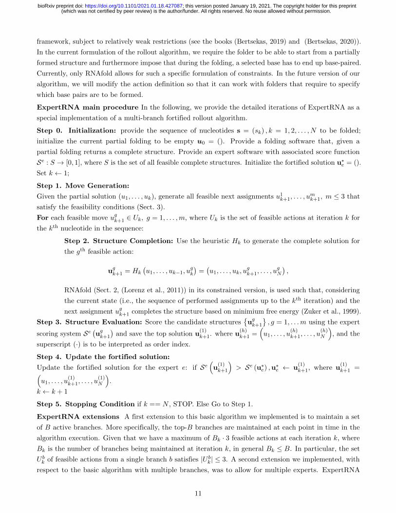
ExpertRNA main procedure In the following, we provide the detailed iterations of ExpertRNA as a

special implementation of a multi-branch fortified rollout algorithm.

Step 0. Initialization: provide the sequence of nucleotides s = (sk) , k = 1, 2, . . . , N to be folded;

initialize the current partial folding to be empty u0 = (). Provide a folding software that, given a

partial folding returns a complete structure. Provide an expert software with associated score function

Se : S → [0, 1], where S is the set of all feasible complete structures. Initialize the fortified solution u∗e = ().

Set k ← 1;

Step 1. Move Generation:

Given the partial solution (u1, . . . , uk), generate all feasible next assignments u1k+1, . . . , umk+1, m ≤ 3 that

satisfy the feasibility conditions (Sect. 3).

For each feasible move ugk+1 ∈ Uk, g = 1, . . . ,m, where Uk is the set of feasible actions at iteration k for

the kth nucleotide in the sequence:

Step 2. Structure Completion: Use the heuristic Hk to generate the complete solution for

the gth feasible action:

ugk+1 = Hk

(u1, . . . , uk−1, u

gk

)=(u1, . . . , uk, u

gk+1, . . . , u

gN

),

RNAfold (Sect. 2, (Lorenz et al., 2011)) in its constrained version, is used such that, considering

the current state (i.e., the sequence of performed assignments up to the kth iteration) and the

next assignment ugk+1 completes the structure based on minimium free energy (Zuker et al., 1999).

Step 3. Structure Evaluation: Score the candidate structures{ugk+1

}, g = 1, . . .m using the expert

scoring system Se(ugk+1

)and save the top solution u

(1)k+1. where u

(h)k+1 =

(u1, . . . , u

(h)k+1, . . . , u

(h)N

), and the

superscript (·) is to be interpreted as order index.

Step 4. Update the fortified solution:

Update the fortified solution for the expert e: if Se(u(1)k+1

)> Se (u∗e) ,u

∗e ← u

(1)k+1, where u

(1)k+1 =

(u1, . . . , u

(1)k+1, . . . , u

(1)N

).

k ← k + 1

Step 5. Stopping Condition if k == N , STOP. Else Go to Step 1.

ExpertRNA extensions A first extension to this basic algorithm we implemented is to maintain a set

of B active branches. More specifically, the top-B branches are maintained at each point in time in the

algorithm execution. Given that we have a maximum of Bk · 3 feasible actions at each iteration k, where

Bk is the number of branches being maintained at iteration k, in general Bk ≤ B. In particular, the set

U bk of feasible actions from a single branch b satisfies |U b

k| ≤ 3. A second extension we implemented, with

respect to the basic algorithm with multiple branches, was to allow for multiple experts. ExpertRNA

11


https://doi.org/10.1101/2021.01.18.427087

is such that B is set to be a multiple of the number of experts. This choice is justified by the fact that

no prior information is available that can help us choosing for which expert we should maintain more

branches. Finally, in case multiple experts are adopted, a number of fortified solutions bounded by the

number of experts is maintained at each iteration. The fortified solution(s) is updated at iteration k, if

a structure with higher reward is identified for any of the experts. Then, at each iteration, a solution

generated by a feasible action is compared to the fortified solution. If no action achieves a better score,

the fortified action is chosen instead.

ExpertRNA move generation A focal aspect of ExpertRNA is the generation of the set of feasible

actions at iteration k, Uk (Step 1, Move Generation in the general ExpertRNA algorithm). In the following,

we detail the procedure for the generation of the feasible actions.

Step 0. Initialization: Iteration index k, partially folded structure u1, . . . , uk, and the unfolded

nucleotide sequence sk+1:N = (sl)Nl=k+1 , sl ∈ {A,U,C,G}. Initialize the set of feasible actions to the empty

set Uk+1 = ∅.Step 1. Action Generation: A feasible action represents the pair of nucleotide and the modality used

to attach the nucleotide to the rest of the sequence. There are three possible actions: (i) open base pair,

which we will refer to as uok+1; (i) close base pair, which we will refer to as uck+1; (ii) and the null action

(i.e., simple sequencing), which we refer to as unk+1 .

Step 3. Feasibility Certification: We will verify whether the actions are feasible.

Open Base pairing: Condition 1: Given the incomplete structure uk, derive ho, i.e., the number of

open base pair that have not been closed. If the size of the remaining sequence satisfies N − k > ho + 4 + 1,

then condition 1 is satisfied, and we generate the set of candidate paired bases for the (k + 1)st base;

Condition 2: If, among the nucleotides to pair, there exist at least one nucleotide that can physically pair

with uok+1, then condition 2 is satisfied;

Condition 3: If all the bases with open brackets uoh, h = 1, . . . , k can close if the (k + 1)st base is not a

closed bracket, then condition 3 is satisfied;

If all conditions are satisfied Uk+1 ← Uk+1 ∪ uok+1.

Close Base pairing: Condition 1: Given the incomplete structure uk+1, derive ho, i.e., the number of

open base pair that have not been closed,if ho. If ho > 0, condition 1 is satisfied.

Condition 2: If there is an open base uoh, h ≤ k − 4 and the nucleotide is compliant with the current base,

Condition 2 is satisfied.

If all conditions are satisfied Uk+1 ← Uk+1 ∪ uck+1.

Null pairing: Condition 1: Given the incomplete structure uk, derive ho, i.e., the number of open base

pair that have not been closed, if ho < N − k − 1, then condition 1 satisfied.

Condition 2: Calculate the number of nucleotides of the whole chain minus the position of last closed

nucleotide, denote this number as rk. If rk + 4 ≥ ho, Condition 2 is satisfied.

Condition 3: If the (k + 1)th nucleotide is unpaired, check whether the whole chain can be completed

complying with feasibility constraints, which means all remaining incomplete open base pairs within the

partial chain uk can be paired using nucleotides which have not yet been assigned (A, U, C, G pairing

constraints considered). If so, Condition 3 is satisfied.

If all conditions are satisfied Uk ← Uk ∪ unk .

12


https://doi.org/10.1101/2021.01.18.427087

(a) (b) (c)

(d) (e) (f )

Figure 4: Examples of feasible and infeasible conditions for action as uok+1, uck+1, and unk+1. The green

circles are the bases within the folded partial chain (the last green circle is the position we are currentlyassigning) and the red part is the unfolded part. The black arcs are implemented pairings whereas the bluearcs are being tested for feasibility. (a) the action uok+1 is feasible. (b) simple sequencing unk+1 is feasible.(c) closing a base pair uck+1 at the position is feasible. (d) opening a base pair uok+1 at the position isinfeasible, since open base pairing condition 1 is violated. (e) sequencing unk at the position is infeasible,since null pairing condition 1 is violated. (f) closing the base pair uck at the position is infeasible, sinceclose base pairing condition 2 is violated.

4 Numerical Results

In this section, we compare the performance of ExpertRNA and RNAfold used in isolation. We highlight

that judging the quality of a proposed structure is generally not a trivial problem, and this is the main

motivation at the basis of data-driven approaches that allow to consider rewards different from free energy.

In this analysis, we will consider the sequence-structure pairs in the data sets as the “ground truth”.

Under this working assumption, the better method is the one which produces a sequence-structure pair

that is more similar to the one in the data base. Similarity measures will be discussed.

4.1 Experimental Setting

Data set for training When training ENTRNA, we adopted 1024 pseudoknot-free RNA molecules from

the RNASTRAND data base (Andronescu et al., 2008). The length of the sequences within the data base

ranges from 4 to 1192 nucleotides (Fig. 5(a) shows the distribution of the sequence length).

0 200 400 600 800 1000 12000

100

200

300

400

500

50 100 150 200 250 300 3500

200

400

600

800

1000

100 200 300 4000

20

40

60

80

100

120

Co

un

t

Co

un

t

Co

un

t

RNA Length RNA Length

(a) (b) (c)

RNA Length

Figure 5: Distribution of RNA length in (a) RNASTRAND, (b) Mathews, and (c) Rfam.

Data set for testing ExpertRNA was tested on two data sets. The first data set was obtained from the

Rfam data base (Burge et al., 2013) by randomly selecting a subset of seed structures from distinct ncRNA

families. Specifically, we used 167 sequences of length ranging from 71 to 408 nucleotides (Fig. 5(c)). The

13


https://doi.org/10.1101/2021.01.18.427087

second data set is the benchmark data set of the RNAStructure tool (Reuter and Mathews, 2010), as

populated by Mathews’ lab (Ward et al., 2017), which consists of natural RNA sequences with known

secondary structures, comprising 1880 sequences of lengths ranging from 28 to 338 nucleotides (Fig. 5(b)).

Metrics As previously mentioned, in this analysis, we consider better the algorithm that produces a

structure that is close to the one in the data base. More specifically, to evaluate the quality of the produced

structures, we look into three indicators:

• Free Energy (FE): Free Energy (FE) is a standard metric to evaluate the quality of an RNA structure.

RNAfold is a FE minimizer. Hence, the ExpertRNA solution may have higher associated FE. The

free energy calculation used here is from the ViennaRNA package and is the same one used by

RNAfold (Lorenz et al., 2011);

• Matthews Correlation Coefficient (MCC): MCC (Matthews, 1975) is a popular metric in the RNA

structure prediction field used to score the confusion matrix of a binary prediction. It takes into

account the number of correctly and incorrectly predicted paired/unpaired bases and returns a

score between -1 and 1, where -1 is a totally incorrect structure, 0 is the expected value of random

assignment and 1 is a totally correct structure. The formal definition is:

MCC =TP · TN − FP · FN√

(TP + FP ) · (TP + FN) · (TN + FP ) · (TN + FN)(4)

where TP, TN are the correctly identified paired and unpaired bases, respectively. FP, FN are the

incorrectly paired and unpaired bases, respectively.

• Foldability: This metric is a score in the interval [0, 1] quantified by ENTRNA. The higher the

foldability the more likely is the sequence-structure pair to fold (Sect. 2).

ExpertRNA Settings We created an extension of ENTRNA for this work, namely, the No Free Energy

ENTRNA (ENTRNA-NFE). Specifically, we re-trained the ENTRNA classifier removing the free energy

from the set of features used to train the Support Vector Machine at the basis of the expert. The rationale

behind this modification was to allow to search for solutions (structures) that do not necessarily have low

free energy. ENTRNA-NFE was a better-performing expert than the original ENTRNA as well as the

ExpertRNA using both ENTRNA and ENTRNA-NFE simultaneously. We ran these several variants of

ExpertRNA maintaining four branches at each iteration. In the case where we used both experts, we

allowed each expert to maintain its two highest scoring branches at each iteration. As a result, at each

iteration k of ExpertRNA, we have a number B = 4 of active branches and B = 4 structure foldings are

performed. To reduce the computational demand, the foldings can be parallelized. All results reported

were obtained from ExpertRNA with ENTRNA-NFE expert. Nonetheless, similar performance were

obtained with the ENTRNA expert and when using both experts together.

4.2 Performance analysis

In the following, we analyse first the MCC as main discerning metric to individuate the characteristics of

the proposed algorithm against the state of the art RNAfold. We then look into free energy and foldability

to provide additional insights on the difference between the two approaches.

14


https://doi.org/10.1101/2021.01.18.427087

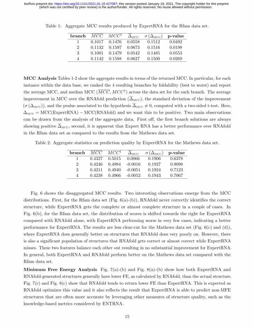
Table 1: Aggregate MCC results produced by ExpertRNA for the Rfam data set.

branch MCC MCC† ∆MCC σ (∆MCC) p-value

1 0.1017 0.1476 0.0558 0.1512 0.04922 0.1132 0.1597 0.0673 0.1516 0.01983 0.1001 0.1479 0.0542 0.1485 0.05534 0.1142 0.1588 0.0627 0.1500 0.0269

MCC Analysis Tables 1-2 show the aggregate results in terms of the returned MCC. In particular, for each

instance within the data base, we ranked the 4 resulting branches by foldability (best to worst) and report

the average MCC, and median MCC (MCC,MCC†) across the data set for the each branch. The average

improvement in MCC over the RNAfold prediction (∆MCC), the standard deviation of the improvement

(σ (∆MCC)), and the pvalue associated to the hypothesis ∆MCC 6= 0, computed with a two-sided t-test. Here,

∆MCC = MCC(ExpertRNA)−MCC(RNAfold) and we want this to be positive. Two main observations

can be drawn from the analysis of the aggregate data. First off, the first branch solutions are always

showing positive ∆MCC, second, it is apparent that Expert RNA has a better performance over RNAfold

in the Rfam data set as compared to the results from the Mathews data set.

Table 2: Aggregate statistics on prediction quality by ExpertRNA for the Mathews data set.

branch MCC MCC† ∆MCC σ (∆MCC) p-value

1 0.4327 0.5015 0.0066 0.1906 0.63782 0.4246 0.4984 -0.0016 0.1927 0.90983 0.4211 0.4940 -0.0051 0.1924 0.71234 0.4238 0.4966 -0.0052 0.1943 0.7067

Fig. 6 shows the disaggregated MCC results. Two interesting observations emerge from the MCC

distributions. First, for the Rfam data set (Fig. 6(a)-(b)), RNAfold never correctly identifies the correct

structure, while ExpertRNA gets the complete or almost complete structure in a couple of cases. In

Fig. 6(b), for the Rfam data set, the distribution of scores is shifted towards the right for ExpertRNA

compared with RNAfold alone, with ExpertRNA performing worse in very few cases, indicating a better

performance for ExpertRNA. The results are less clear-cut for the Mathews data set (Fig. 6(c) and (d)),

where ExpertRNA does generally better on structures that RNAfold does very poorly on. However, there

is also a significant population of structures that RNAfold gets correct or almost correct while ExpertRNA

misses. These two features balance each other out resulting in no substantial improvement for ExpertRNA.

In general, both ExpertRNA and RNAfold perform better on the Mathews data set compared with the

Rfam data set.

Minimum Free Energy Analysis Fig. 7(a)-(b) and Fig. 8(a)-(b) show how both ExpertRNA and

RNAfold-generated structures generally have lower FE, as calculated by RNAfold, than the actual structure.

Fig. 7(c) and Fig. 8(c) show that RNAfold tends to return lower FE than ExpertRNA. This is expected as

RNAfold optimizes this value and it also reflects the result that ExpertRNA is able to predict non-MFE

structures that are often more accurate by leveraging other measures of structure quality, such as the

knowledge-based metrics considered by ENTRNA.

15


https://doi.org/10.1101/2021.01.18.427087

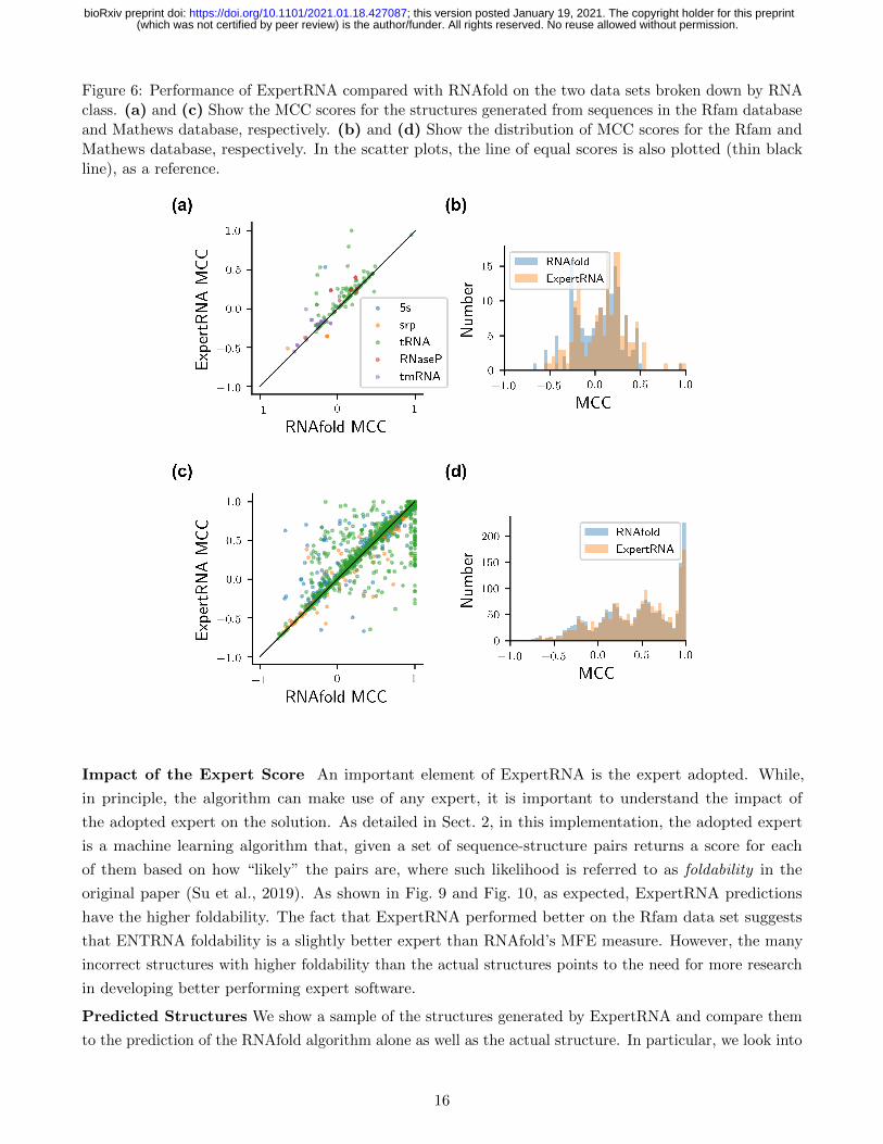
Figure 6: Performance of ExpertRNA compared with RNAfold on the two data sets broken down by RNAclass. (a) and (c) Show the MCC scores for the structures generated from sequences in the Rfam databaseand Mathews database, respectively. (b) and (d) Show the distribution of MCC scores for the Rfam andMathews database, respectively. In the scatter plots, the line of equal scores is also plotted (thin blackline), as a reference.

Impact of the Expert Score An important element of ExpertRNA is the expert adopted. While,

in principle, the algorithm can make use of any expert, it is important to understand the impact of

the adopted expert on the solution. As detailed in Sect. 2, in this implementation, the adopted expert

is a machine learning algorithm that, given a set of sequence-structure pairs returns a score for each

of them based on how “likely” the pairs are, where such likelihood is referred to as foldability in the

original paper (Su et al., 2019). As shown in Fig. 9 and Fig. 10, as expected, ExpertRNA predictions

have the higher foldability. The fact that ExpertRNA performed better on the Rfam data set suggests

that ENTRNA foldability is a slightly better expert than RNAfold’s MFE measure. However, the many

incorrect structures with higher foldability than the actual structures points to the need for more research

in developing better performing expert software.

Predicted Structures We show a sample of the structures generated by ExpertRNA and compare them

to the prediction of the RNAfold algorithm alone as well as the actual structure. In particular, we look into

16


https://doi.org/10.1101/2021.01.18.427087

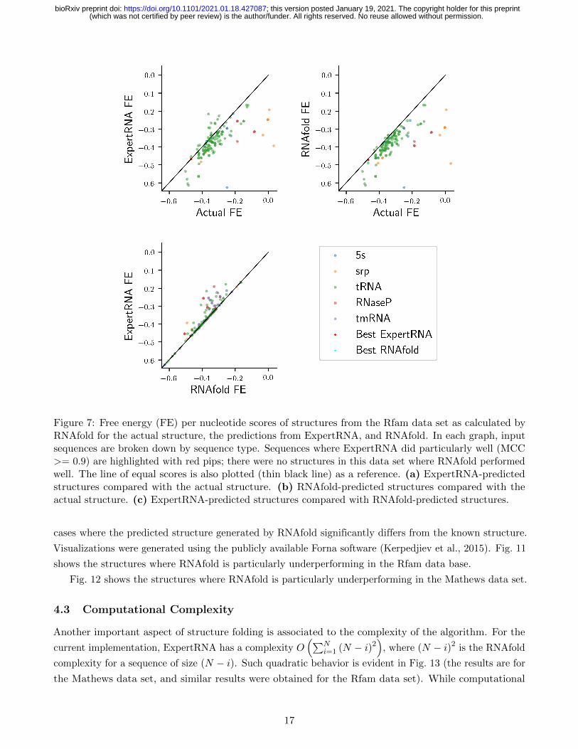
Figure 7: Free energy (FE) per nucleotide scores of structures from the Rfam data set as calculated byRNAfold for the actual structure, the predictions from ExpertRNA, and RNAfold. In each graph, inputsequences are broken down by sequence type. Sequences where ExpertRNA did particularly well (MCC>= 0.9) are highlighted with red pips; there were no structures in this data set where RNAfold performedwell. The line of equal scores is also plotted (thin black line) as a reference. (a) ExpertRNA-predictedstructures compared with the actual structure. (b) RNAfold-predicted structures compared with theactual structure. (c) ExpertRNA-predicted structures compared with RNAfold-predicted structures.

cases where the predicted structure generated by RNAfold significantly differs from the known structure.

Visualizations were generated using the publicly available Forna software (Kerpedjiev et al., 2015). Fig. 11

shows the structures where RNAfold is particularly underperforming in the Rfam data base.

Fig. 12 shows the structures where RNAfold is particularly underperforming in the Mathews data set.

4.3 Computational Complexity

Another important aspect of structure folding is associated to the complexity of the algorithm. For the

current implementation, ExpertRNA has a complexity O(∑N

i=1 (N − i)2)

, where (N − i)2 is the RNAfold

complexity for a sequence of size (N − i). Such quadratic behavior is evident in Fig. 13 (the results are for

the Mathews data set, and similar results were obtained for the Rfam data set). While computational

17


https://doi.org/10.1101/2021.01.18.427087

Figure 8: Free energy (FE) of structures from the Mathews database as calculated by RNAfold calculatedfor the actual structure, and the predictions from ExpertRNA, and RNAfold. In each graph, inputsequences are broken down by sequence type. Sequences where ExpertRNA and RNAfold did particularlywell (MCC >= 0.9) are highlighted with smaller cyan and red pips, respectively. The line of equalscores is also plotted (thin black line) as a reference. (a) ExpertRNA-predicted structures comparedwith the actual structure. (b) RNAfold-predicted structures compared with the actual structure. (c)ExpertRNA-predicted structures compared with RNAfold-predicted structures.

efficiency is a known challenge in secondary structure prediction, a promising avenue will be to investigate

multi-agent rollout (Bertsekas, 2020) as a way to boost the efficiency.

4.4 Summary

Compared to the RNAfold tool, ExpertRNA performs better on the data set of known structures from

Rfam, and approximately equivalently on the data set from the Mathews lab. In several cases, the

ExpertRNA structures had higher free energy (compared to RNAfold) according to the nearest-neighbor

model. However, they are closer to the actual known structure. Structures predicted by both ExpertRNA

and RNAfold almost always have lower free energy than the actual structure, further indicating the

limitations of free energy approximations in identifying correctly folded structures. In most cases, where

18


https://doi.org/10.1101/2021.01.18.427087

Figure 9: Foldability scores for structure predictions from the Rfam data set as calculated by the expert,ENTRNA-NFE. In each graph, input sequences are broken down by sequence type. Sequences whereExpertRNA did particularly well (MCC >= 0.9) are highlighted with red pips; there were no structuresin this data set where RNAfold performed well. The line of equal scores is also plotted (thin black line)as a reference. (a) ExpertRNA-predicted structures compared with the actual structure. (b) RNAfold-predicted structures compared with the actual structure. (c) ExpertRNA-predicted structures comparedwith RNAfold-predicted structures.

ExpertRNA found structure in better agreement with the actual known structure, the FE of that structure

was only slightly higher than the FE of RNAfold. However, in few cases (e.g. Fig. 12(a)-(c),(g)-(i)), the

solutions where ExpertRNA had much better agreement with the correct structure, RNAfold solution had

much lower free energy. ExpertRNA hence shows the ability to identify the correct structure even if its

predicted FE is quite higher than the MFE prediction by integrating other experts that may implicitly or

explicitly account tertiary contact and kinetic information.

5 Conclusions

In this paper, we propose a new framework, ExpertRNA, for the automatic folding of secondary structures

for RNA molecular compounds. ExpertRNA builds upon the fortified rollout algorithm and generalizes

19


https://doi.org/10.1101/2021.01.18.427087

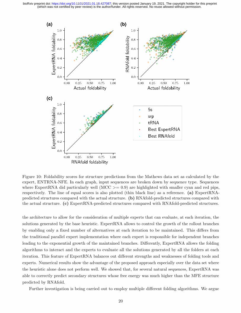
Figure 10: Foldability scores for structure predictions from the Mathews data set as calculated by theexpert, ENTRNA-NFE. In each graph, input sequences are broken down by sequence type. Sequenceswhere ExpertRNA did particularly well (MCC >= 0.9) are highlighted with smaller cyan and red pips,respectively. The line of equal scores is also plotted (thin black line) as a reference. (a) ExpertRNA-predicted structures compared with the actual structure. (b) RNAfold-predicted structures compared withthe actual structure. (c) ExpertRNA-predicted structures compared with RNAfold-predicted structures.

the architecture to allow for the consideration of multiple experts that can evaluate, at each iteration, the

solutions generated by the base heuristic. ExpertRNA allows to control the growth of the rollout branches

by enabling only a fixed number of alternatives at each iteration to be maintained. This differs from

the traditional parallel expert implementation where each expert is responsible for independent branches

leading to the exponential growth of the maintained branches. Differently, ExpertRNA allows the folding

algorithms to interact and the experts to evaluate all the solutions generated by all the folders at each

iteration. This feature of ExpertRNA balances out different strengths and weaknesses of folding tools and

experts. Numerical results show the advantage of the proposed approach especially over the data set where

the heuristic alone does not perform well. We showed that, for several natural sequences, ExpertRNA was

able to correctly predict secondary structures whose free energy was much higher than the MFE structure

predicted by RNAfold.

Further investigation is being carried out to employ multiple different folding algorithms. We argue

20


https://doi.org/10.1101/2021.01.18.427087

Figure 11: Example structure from the Rfam data set with the best performance improvement betweenExpertRNA and RNAfold. Each row contains the actual structure (a-d-g), the RNAfold (b-e-h), and theExpertRNA prediction (c-f-i). Nucleotides whose pairing was predicted incorrectly are shown in red inpanels (b) and (c), while correct pairings are green. The numbers in parenthesis are: foldability of thestructure as evaluated by ENTRNA-NFE, free energy as evaluated by RNAfold, and MCC compared withthe actual structure (bold): (a-c) A phenylalanine tRNA from Archaeoglobus fulgidis; (d-f) An alaninetRNA from Methanococcus maripaludis; (g-i) A 5s rRNA from Bacillus toyonensis.

that, in the process of generating the solution, perhaps one of the folders will be performing very well, but,

after some iterations, a different folder may produce superior results. In some sense, ExpertRNA tracks

the best folder, online, as the sequence is being constructed. Also, we are investigating the opportunity

to use more/different experts. In light of this, a possible future direction is to include more features in

ENTRNA training or combination with additional expert scoring (e.g., based on covariation information

21


https://doi.org/10.1101/2021.01.18.427087

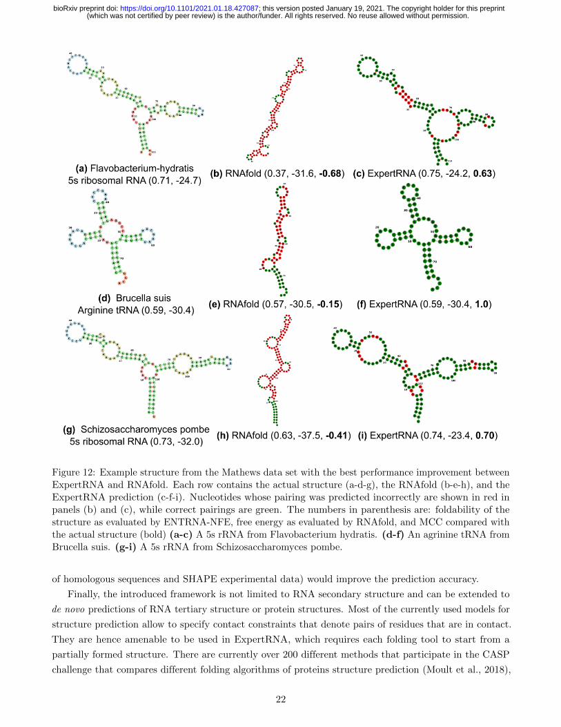
Figure 12: Example structure from the Mathews data set with the best performance improvement betweenExpertRNA and RNAfold. Each row contains the actual structure (a-d-g), the RNAfold (b-e-h), and theExpertRNA prediction (c-f-i). Nucleotides whose pairing was predicted incorrectly are shown in red inpanels (b) and (c), while correct pairings are green. The numbers in parenthesis are: foldability of thestructure as evaluated by ENTRNA-NFE, free energy as evaluated by RNAfold, and MCC compared withthe actual structure (bold) (a-c) A 5s rRNA from Flavobacterium hydratis. (d-f) An agrinine tRNA fromBrucella suis. (g-i) A 5s rRNA from Schizosaccharomyces pombe.

of homologous sequences and SHAPE experimental data) would improve the prediction accuracy.

Finally, the introduced framework is not limited to RNA secondary structure and can be extended to

de novo predictions of RNA tertiary structure or protein structures. Most of the currently used models for

structure prediction allow to specify contact constraints that denote pairs of residues that are in contact.

They are hence amenable to be used in ExpertRNA, which requires each folding tool to start from a

partially formed structure. There are currently over 200 different methods that participate in the CASP

challenge that compares different folding algorithms of proteins structure prediction (Moult et al., 2018),

22


https://doi.org/10.1101/2021.01.18.427087

Figure 13: Computational effort for ExpertRNA across the Mathews data set with quadratic fit shown.

and over 10 different methods in its RNA counterpart, RNA-puzzle (Cruz et al., 2012), and these algorithms

can be used as folders in the Expert-RNA framework. The experts in such implementation can correspond

to the system energy calculated, e.g., with Rosetta (Rohl et al., 2004), and other knowledge-based

potentials. The Expert-RNA tool is freely available at https://github.com/MenghanLiu212/RL-RNA,

and the scripts used to process the output of Expert-RNA into Fig. 6-12 are freely available at https:

//github.com/ErikPoppleton/rollout_plotter.

References

Aghaeepour, N., and H. H. Hoos. 2013. “Ensemble-based prediction of RNA secondary structures”. BMC

bioinformatics 14 (1): 139.

Andronescu, M., V. Bereg, H. H. Hoos, and A. Condon. 2008. “RNA STRAND: the RNA secondary

structure and statistical analysis database”. BMC bioinformatics 9 (1): 1.

Andronescu, M., A. Condon, H. H. Hoos, D. H. Mathews, and K. P. Murphy. 2007. “Efficient parameter

estimation for RNA secondary structure prediction”. Bioinformatics 23 (13): i19–i28.

Andronescu, M., A. Condon, H. H. Hoos, D. H. Mathews, and K. P. Murphy. 2010. “Computational

approaches for RNA energy parameter estimation”. RNA 16 (12): 2304–2318.

Angela, M. Y., P. M. Gasper, E. J. Strobel, K. E. Watters, A. A. Chen, and J. B. Lucks. 2018. “Compu-

tationally Reconstructing Cotranscriptional RNA Folding Pathways from Experimental Data Reveals

Rearrangement of Non-Native Folding Intermediates”. bioRxiv :379222.

Antczak, M., M. Popenda, T. Zok, M. Zurkowski, R. W. Adamiak, and M. Szachniuk. 2018. “New algorithms

to represent complex pseudoknotted RNA structures in dot-bracket notation”. Bioinformatics 34 (8):

1304–1312.

Bertsekas, D. . P. 2019. Reinforcement Learning and Optimal Control. Athena Scientific, Belmont, MA.

Bertsekas, D. . P. 2020. Rollout, Policy Iteration, and Distributed Reinforcement Learning. Athena

Scientific, Belmont, MA.

23


https://github.com/MenghanLiu212/RL-RNA

https://github.com/ErikPoppleton/rollout_plotter

https://github.com/ErikPoppleton/rollout_plotter

https://doi.org/10.1101/2021.01.18.427087

Bertsekas, D. P., and J. N. Tsitsiklis. 1996. Neuro-Dynamic Programming. Athena Scientific, Belmont,

MA.

Bertsekas, D. P., J. N. Tsitsiklis, and C. Wu. 1997. “Rollout algorithms for combinatorial optimization”.

Journal of Heuristics 3 (3): 245–262.

Burge, S. W., J. Daub, R. Eberhardt, J. Tate, L. Barquist, E. P. Nawrocki, S. R. Eddy, P. P. Gardner, and

A. Bateman. 2013. “Rfam 11.0: 10 years of RNA families”. Nucleic acids research 41 (D1): D226–D232.

Calonaci, N., A. Jones, F. Cuturello, M. Sattler, and G. Bussi. 2020. “Machine learning a model for RNA

structure prediction”. arXiv preprint arXiv:2004.00351 .

Chowdhury, F. R. R., H. Zhang, and L. Huang. 2019. “Learning to Fold RNAs in Linear Time”.

bioRxiv :852871.

Cruz, J. A., M.-F. Blanchet, M. Boniecki, J. M. Bujnicki, S.-J. Chen, S. Cao, R. Das, F. Ding, N. V.

Dokholyan, S. C. Flores et al. 2012. “RNA-Puzzles: a CASP-like evaluation of RNA three-dimensional

structure prediction”. Rna 18 (4): 610–625.

Dieckmann, T., E. Suzuki, G. K. Nakamura, and J. Feigon. 1996. “Solution structure of an ATP-binding

RNA aptamer reveals a novel fold.”. Rna 2 (7): 628–640.

Do, C. B., D. A. Woods, and S. Batzoglou. 2006. “CONTRAfold: RNA secondary structure prediction

without physics-based models”. Bioinformatics 22 (14): e90–e98.

Elliott, D., and M. Ladomery. 2017. Molecular biology of RNA. Oxford University Press.

Geary, C., P. W. Rothemund, and E. S. Andersen. 2014. “A single-stranded architecture for cotranscriptional

folding of RNA nanostructures”. Science 345 (6198): 799–804.

Green, A. A., P. A. Silver, J. J. Collins, and P. Yin. 2014. “Toehold switches: de-novo-designed regulators

of gene expression”. Cell 159 (4): 925–939.

Guo, P. 2010. “The emerging field of RNA nanotechnology”. Nature nanotechnology 5 (12): 833.

Han, D., X. Qi, C. Myhrvold, B. Wang, M. Dai, S. Jiang, M. Bates, Y. Liu, B. An, F. Zhang et al. 2017.

“Single-stranded DNA and RNA origami”. Science 358 (6369): eaao2648.

Hanson, J., T. Litfin, K. Paliwal, and Y. Zhou. 2020. “Identifying molecular recognition features in

intrinsically disordered regions of proteins by transfer learning”. Bioinformatics 36 (4): 1107–1113.

Hochrein, L. M., M. Schwarzkopf, M. Shahgholi, P. Yin, and N. A. Pierce. 2013. “Conditional Dicer

substrate formation via shape and sequence transduction with small conditional RNAs”. Journal of the

American Chemical Society 135 (46): 17322–17330.

Hofacker, I. L. 2003. “Vienna RNA secondary structure server”. Nucleic acids research 31 (13): 3429–3431.

Isambert, H., and E. D. Siggia. 2000. “Modeling RNA folding paths with pseudoknots: application to

hepatitis delta virus ribozyme”. PNAS 97 (12): 6515–6520.

24


https://doi.org/10.1101/2021.01.18.427087

Kerpedjiev, P., S. Hammer, and I. L. Hofacker. 2015. “Forna (force-directed RNA): Simple and effective

online RNA secondary structure diagrams”. Bioinformatics 31 (20): 3377–3379.

Li, X.-L., P. S. Yu, B. Liu, and S.-K. Ng. 2009. “Positive unlabeled learning for data stream classification”.

In Proceedings of the 2009 SIAM International Conference on Data Mining, 259–270. SIAM.

Lorenz, R., S. H. Bernhart, C. H. Zu Siederdissen, H. Tafer, C. Flamm, P. F. Stadler, and I. L. Hofacker.

2011. “ViennaRNA Package 2.0”. Algorithms for molecular biology 6 (1): 26.

Low, J. T., and K. M. Weeks. 2010. “SHAPE-directed RNA secondary structure prediction”. Methods 52

(2): 150–158.

Lucks, J. B., S. A. Mortimer, C. Trapnell, S. Luo, S. Aviran, G. P. Schroth, L. Pachter, J. A. Doudna, and

A. P. Arkin. 2011. “Multiplexed RNA structure characterization with selective 2’-hydroxyl acylation

analyzed by primer extension sequencing (SHAPE-Seq)”. Proceedings of the National Academy of

Sciences 108 (27): 11063–11068.

Mathews, D. H., J. Sabina, M. Zuker, and D. H. Turner. 1999. “Expanded sequence dependence of

thermodynamic parameters improves prediction of RNA secondary structure”. Journal of molecular

biology 288 (5): 911–940.

Matthews, B. W. 1975. “Comparison of the predicted and observed secondary structure of T4 phage

lysozyme”. Biochimica et Biophysica Acta (BBA)-Protein Structure 405 (2): 442–451.

Miao, Z., R. W. Adamiak, M. Antczak, R. T. Batey, A. J. Becka, M. Biesiada, M. J. Boniecki, J. M.

Bujnicki, S.-J. Chen, C. Y. Cheng et al. 2017. “RNA-Puzzles Round III: 3D RNA structure prediction

of five riboswitches and one ribozyme”. Rna 23 (5): 655–672.

Moult, J., K. Fidelis, A. Kryshtafovych, T. Schwede, and A. Tramontano. 2018. “Critical assessment of

methods of protein structure prediction (CASP)—Round XII”. Proteins: Structure, Function, and

Bioinformatics 86:7–15.

Qi, X., X. Liu, L. Matiski, R. Rodriguez Del Villar, T. Yip, F. Zhang, S. Sokalingam, S. Jiang, L. Liu,

H. Yan et al. 2020. “RNA Origami Nanostructures for Potent and Safe Anticancer Immunotherapy”.

ACS nano 14 (4): 4727–4740.

Reuter, J. S., and D. H. Mathews. 2010. “RNAstructure: software for RNA secondary structure prediction

and analysis”. BMC bioinformatics 11 (1): 129.

Rohl, C. A., C. E. Strauss, K. M. Misura, and D. Baker. 2004. “Protein structure prediction using Rosetta”.

In Methods in enzymology, Volume 383, 66–93. Elsevier.

Seetin, M. G., and D. H. Mathews. 2011. “Automated RNA tertiary structure prediction from secondary

structure and low-resolution restraints”. Journal of computational chemistry 32 (10): 2232–2244.

Singh, J., J. Hanson, K. Paliwal, and Y. Zhou. 2019. “RNA secondary structure prediction using an

ensemble of two-dimensional deep neural networks and transfer learning”. Nature communications 10

(1): 1–13.

25


https://doi.org/10.1101/2021.01.18.427087

Sloma, M. F., and D. H. Mathews. 2017. “Base pair probability estimates improve the prediction accuracy

of RNA non-canonical base pairs”. PLoS computational biology 13 (11): e1005827.

Su, C., J. D. Weir, F. Zhang, H. Yan, and T. Wu. 2019. “ENTRNA: a framework to predict RNA

foldability”. BMC bioinformatics 20 (1): 373.

Sun, T.-t., C. Zhao, and S.-J. Chen. 2018. “Predicting Cotranscriptional Folding Kinetics For Riboswitch”.

The Journal of Physical Chemistry B 122 (30): 7484–7496.

Tan, Z.-J., and S.-J. Chen. 2010. “Predicting ion binding properties for RNA tertiary structures”.

Biophysical journal 99 (5): 1565–1576.

Wang, L., Y. Liu, X. Zhong, H. Liu, C. Lu, C. Li, and H. Zhang. 2019. “DMFold: A novel method to

predict RNA secondary structure with pseudoknots based on deep learning and improved base pair

maximization principle”. Frontiers in genetics 10:143.

Ward, M., A. Datta, M. Wise, and D. H. Mathews. 2017. “Advanced multi-loop algorithms for RNA

secondary structure prediction reveal that the simplest model is best”. Nucleic acids research 45 (14):

8541–8550.

Watkins, A. M., R. Rangan, and R. Das. 2020. “FARFAR2: Improved de novo Rosetta prediction of

complex global RNA folds”. Structure.

Wayment-Steele, H. K., W. Kladwang, E. Participants, and R. Das. 2020. “RNA secondary structure

packages ranked and improved by high-throughput experiments”. BioRxiv .

Westhof, E., and P. Auffinger. 2006. “RNA tertiary structure”. Encyclopedia of Analytical Chemistry:

Applications, Theory and Instrumentation.

Xia, T., J. SantaLucia Jr, M. E. Burkard, R. Kierzek, S. J. Schroeder, X. Jiao, C. Cox, and D. H. Turner.

1998. “Thermodynamic parameters for an expanded nearest-neighbor model for formation of RNA

duplexes with Watson- Crick base pairs”. Biochemistry 37 (42): 14719–14735.

Zadeh, J. N., C. D. Steenberg, J. S. Bois, B. R. Wolfe, M. B. Pierce, A. R. Khan, R. M. Dirks, and

N. A. Pierce. 2011. “NUPACK: analysis and design of nucleic acid systems”. Journal of computational

chemistry 32 (1): 170–173.

Zuker, M., D. H. Mathews, and D. H. Turner. 1999. “Algorithms and thermodynamics for RNA secondary

structure prediction: a practical guide”. In RNA biochemistry and biotechnology, 11–43. Springer.

Zuker, M., and P. Stiegler. 1981. “Optimal computer folding of large RNA sequences using thermodynamics

and auxiliary information”. Nucleic acids research 9 (1): 133–148.

26


https://doi.org/10.1101/2021.01.18.427087

expertrna: a new framework for rna structure prediction

Documents