expert systems with applications -...

Expert Systems with Applications 38 (2011) 14819–14831

Contents lists available at ScienceDirect

Expert Systems with Applications

journal homepage: www.elsevier .com/locate /eswa

Cost optimization of integrated network planning based on adaptive sectorizationin hybrid F/CDMA telecommunications system via Lagrangean relaxation

Kuo-Chung Chu a, Frank Yeong-Sung Lin b, Chun-Sheng Wang c,⇑

a Department of Information Management, National Taipei University of Nursing and Health Sciences, 365, Min-Te Road, Taipei, Taiwan, ROCb Department of Information Management, National Taiwan University, 1, Sec. 4, Roosevelt Rd., Taipei, Taiwan, ROCc Department of Information Management, Jinwen University of Science and Technology, 99, An-Chung Road, Hsin-Tien, Taipei, Taiwan, ROC

a r t i c l e i n f o

Keywords:CDMACombinatorial optimizationHybrid F/CDMA schemeLagrangean relaxationNetwork planningNetwork survivabilitySectorization

0957-4174/$ - see front matter � 2011 Elsevier Ltd. Adoi:10.1016/j.eswa.2011.05.067

⇑ Corresponding author.E-mail addresses: [email protected] (K.-C. Chu

Lin), [email protected], [email protected]

a b s t r a c t

In this paper, we investigate the integrated network planning for telecommunications system, which con-siders adaptive sectorization and a hybrid F/CDMA scheme jointly under quality of service (QoS) con-straints. The problem is formulated as a combinatorial optimization formulation in terms ofminimizing the cost. We also investigate the viability of using Lagrangean relaxation (LR) to solve theproblem. With regard to the computational results, the cost of considering network error states in theplanning stage is 45% more than that of non-error. The proposed LR approach outperforms a simple algo-rithm with a cost improvement of 60%. In addition, the link constraint is more important to the total costthan the node constraint. Given a link constraint, the cost is affected more significantly by a decreasingthreshold than by an increasing threshold. The proposed model is not only a valuable reference for net-work planning in a new field (e.g., a desert scenario), but also fits the planning requirements when someequipment pre-exists (an embedded scenario). We assign constant values to several decision variables, sothe model is adaptable to various scenarios.

� 2011 Elsevier Ltd. All rights reserved.

1. Introduction key factor in the routing problem, the backbone topology and the

1.1. Challenges of integrated network planning

The use of wireless communications continues to experiencedramatic growth. While voice services are now almost ubiquitous,wireless data applications have only recently gained momentum.The ongoing migration of voice services from wired to wireless sys-tems, as well as the ever-increasing number of data applications,figure prominently in the drive toward fulfillment of code divisionmultiple access (CDMA)-based 3G systems and beyond. Generally,wireless cellular network planning involves both wireline andwireless (radio) elements. Fig. 1 shows the system architecture ofan integrated wireline/wireless network. In wireline networks,planning issues include mobile switching center (MSC) allocation,MSC interconnection, base station (BS) allocation or cell placement,BS configuration (cell sectorization), backbone topology, and trafficrouting. The MSC serves as the access point for the wireless net-work to connect to the wireline backbone network. A number ofwireless networks, i.e., radio access networks (RANs), are con-nected to the MSC. The coverage of a RAN consists of several cells,each of which is served by a BS. Since the backbone topology is a

ll rights reserved.

), [email protected] (F.Y.-S.(C.-S. Wang).

routing path for each origin–destination (OD) pair must be consid-ered jointly. Meanwhile, in a wireless system, channel (spectrum)assignment, BS power control, and mobile station/mobile user(MS/MU, the two terms are used interchangeably hereafter) hom-ing must be considered. For each MU, the BS is the first tier facilityfor accessing the network (RAN). Generally speaking, hundreds tothousands of users are covered/served by the BSs, so those userswould be out of service if a RAN were to fail. Thus, network surviv-ability is very important in the planning of RANs.

The survivability of telecommunication networks is a crucial is-sue for both service providers and end users. Actually, the problemof network survivability stems from network planning. The plan-ning process can be categorized into the three phases: topologicaldesign, traffic routing, and circuit routing design in the transmis-sion facility network (Medhi, 1994). In traffic routing, for example,the primary goal is to provide optimal capacity with quality of ser-vice (QoS) guarantees, while minimum-cost routing is primarilyconcerned with circuit routing design.

Network failures can occur as a result of natural disasters(floods, hurricanes, etc.), human actions (war, terrorism, hacker at-tacks) or the failure of software or control systems. The networkmust be designed for survivability, so that traffic can still be carriedimmediately after a failure. Efforts should focus on designing net-works so that service can be maintained at a reasonable cost ifthere is a failure. A wireless or mobile network consists of a

http://dx.doi.org/10.1016/j.eswa.2011.05.067

mailto:[email protected]




http://dx.doi.org/10.1016/j.eswa.2011.05.067

http://www.sciencedirect.com/science/journal/09574174

http://www.elsevier.com/locate/eswa

Wireline Backbone Network

MSC MSC

MSC

RAN

RAN

RAN

RAN

Mobile Switching Center

Radio Access Network

Base Station

Mobile Station

Wireline Link

Wireless Link

MSCHome Location Register (HLR) /Visitor Location Register (VLR)

Fig. 1. System architecture of an integrated wireline/wireless network.

Table 1The effects of wireless component failure and mitigation strategies.

Failure Cause Number of usersaffected

Time to fix Ways to reduce the risk of failure Time to fix afterimprovements

MSC Hardware, software, operators 100,000 Hours to days Spare components, extra power, smallerswitches, Sonet ring, training

Seconds to minutes

HLR/VLR Hardware, software 100,000 Hours to days Replicated database, redundant components Seconds to minutesBS/BSC Hardware, software, nature 1000 � 20,000 Hours to days Overlay BS, redundant components, Sonet ring Seconds to minutesDevice interface Hardware 1 Hours to days Multiple interfaces, access different wireless

networksSeconds to minutes

14820 K.-C. Chu et al. / Expert Systems with Applications 38 (2011) 14819–14831

number of components, such as BSs, BS controllers (BSCs), MSCs,home location registers (HLRs) and visiting location registers(VLRs), signaling system 7 (SS7), and high-capacity trunks. A failurecould involve one or more of these components, so survivability isalso an important research issue in mobile wireless networks (Chu-prun & Bergstrom, 1998; Snow, Varshney, & Malloy, 2000). The im-pact of a failure can be measured in terms of the number of usersaffected and the duration of the outage. Table 1 summarizes the ef-fects of failures and the mitigation strategies applied in a wirelessenvironment (Snow et al., 2000). To provide reliable and survivablewireless and mobile services, network providers must devise waysto reduce the number of network failures and ways to cope withfailures when they do occur. In the scenario of BS failure, redun-dant components and overlaying BSs can be considered jointly inthe network planning stage (Chu & Lin, 2006).

1.2. Approaches of capacity management

Call admission control (CAC) is a popular mechanism to admitas many users as possible so that the system benefit can be opti-mized (Chu, Wang, & Lin, 2010), while CAC-based adaptive channelreservation approach is proposed for priority soft handoff (Chu,Hung, & Lin, 2009). In addition, cell sectorization is widely usedto increase system capacity in cellular systems. Basically, systemcapacity is considered as a multiple factor that is equal to the num-ber of sectors. This is the case in an ideal antenna system, but dueto the non-ideal antenna radiation pattern, the sectorization gain is

smaller than the number of sectors in reality (Castañeda-Camacho,Uc-Rios, & Lara-Rodríguez, 2003; Wibisono & Darsilo, 2001). Thegain is approximately 2.39 for a non-ideal antenna pattern (Castañ-eda-Camacho et al., 2003). Even if the cell is not uniformly sector-ized, sectorization still helps increase the system capacity(Wibisono & Darsilo, 2001). However, many studies that evaluatethe capacity of CDMA systems assume a uniform spatial traffic dis-tribution, as it best fits CDMA’s characteristics if all signals sharethe whole spectral resource (Liberti & Rappaport, 1994; Wu,Chung, & Sze, 1997). The whole bandwidth is divided equallyamong the cells, so that cells with the heaviest loads have the samefrequency resources as any other cell. Nevertheless, uniformly dis-tributed traffic among cells (equal cell loads) is very uncommon,especially in an urban environment, where the traffic distributionis usually non-uniform.

Although non-uniform traffic reduces the system capacity, veryfew works have considered the problem in conjunction with net-work planning (Tutschku & Tran-Gia, 1998; Wu et al., 1997). Evenif sufficient capacity is planned, uneven/non-uniform (the twoterms are used interchangeably hereafter) traffic distributionmay occur in a cellular system, creating a ‘‘hot spot’’ that exceedsthe pre-determined capacity and introducing a large call blockingprobability. For non-uniform traffic distributions, adaptive sector-ization is an effective way to maximize the network capacity(Lee, Kang, & Park, 2002; Saraydar & Yener, 2001). Sectors are ro-tated and resized adaptively to improve the system’s performancewhen traffic is not uniformly distributed. These studies consider

K.-C. Chu et al. / Expert Systems with Applications 38 (2011) 14819–14831 14821

sectorization as a optimization problem. In Saraydar and Yener(2001), given the number of sectors and MS locations, the objectiveis to minimize the total power consumed by a cell, subject to QoSrequirements. Meanwhile the sectorization problem is formulatedas an integer linear programming model in which the objective isto minimize call blocking for handoff calls between cells in thesame sector (Lee et al., 2002).

Although sectorization is widely used to increase systemcapacity, the communications quality expressed by the signal-to-interference ratio (SIR) differs between cells due to the diversityof the traffic distribution. The variance in communications qualitydegrades the efficiency of spectrum reuse by the whole system. Aprevious work on non-uniform traffic in CDMA (Takeo, Sato, &Ogawa, 1999) dealt with the imbalance of load levels among cells.When non-uniform traffic distribution occurs, it is desirable to re-allocate the radio resources to allow all cells to carry the desiredamount of traffic. Since the ability to accommodate the expectedgrowth in traffic and broadband services is limited by the scarceradio spectrum, it is necessary to design a more spectral efficienttechnique, such as spectrum resource management. In Zhuge andLi (2002, 2003), capacity analysis in multi-band overlaid CDMA isproposed as a way to maximize spectrum utilization. More specifi-cally, the multi-band spectrum is used to meet heterogeneousrequirements. Combining traditional FDMA with CDMA is an alter-native strategy that mitigates interference moderately. Kim andPrabhu (1998) show that the current frequency reuse factor of 1is not always optimal. Meanwhile, the results in Hamidian andPayne (1997) demonstrate that it is possible to increase cell capac-ity without deploying additional cells by applying proper FDMAfrequency reuse to minimize interference. In addition, the adaptivesectorization scheme is also applied to balance the system load in ascenario of non-uniform distributions.

1.3. Complexity of integrated network planning

Mobile network planning involves a sequence of tasks startingfrom coverage analysis and ending with channel assignment. Weneed to determine the amount of network equipment (e.g. MSCs,BSs) required and find suitable placements for the different compo-nents. Effective planning has a significant impact on costs and thequality of service (QoS), as the operator has to assign channels tothe BSs such that QoS is guaranteed. Even though cell planning isa basic task, it is subject to several constraints (Merchant & Seng-upta, 1995; Pierre & Houeto, 2002). In addition, network planningrequires a large number of algorithms, each of which focuses on aproblem with specific constraints. A quite common task is thenecessity to trade-off all design objectives against each other,while respecting their individual importance. Thus, integrated net-work planning becomes a combinatorial optimization problemcomprised of several issues, such as network planning (Ali, 2002;Garg, Simha, & Xing, 2002; Hao et al., 1997; Tutschku, 1998), sur-vivability requirements (Ghashghai & Rardin, 2002), and channelassignment (Duque-Anton, Kunz, & Ruber, 1993; Wang & Rush-forth, 1992), which are NP-complete or NP-hard.

Since the network planning problem is NP-complete, its solu-tion is difficult, even if we succeed in formulating the planningproblem as an optimization task. Although there has been a greatdeal of research into exact algorithms that work for small- andmedium-size problems, the proposed solutions for large-scaleproblems are only approximations. Model developers must makea lot of important planning decisions by deciding which aspectsto include in a model and which aspects to leave out. As a result,developing a very accurate model or trying to reach the exact opti-mum is not a very practical goal. It can even be risky because, whena network is optimized very tightly to achieve one goal, typicallyprofit, it might be expensive to adapt the network to changing

needs. Therefore, instead of trying to find optimal solutions, plan-ning models should allow the user to understand a network’sbehavior and trade-offs better.

For most problems, there is no known algorithm that guaran-tees finding a global optimum in polynomial time. In many cases,sophisticated heuristics have to be developed to achieve satisfac-tory results. The exact solution is practically impossible to achievedue to an exponentially growing calculation time. Moreover, exist-ing heuristics do not guarantee convergence to a truly global opti-mal solution, and the use of non-global optimal solutions wouldprobably lead to significant unwarranted costs in networkplanning.

Traditional planning models that use 2G cellular systems arenot suitable for 3G systems, since they do not consider QoS, powercontrol, or traffic diversity (Amaldi, Capone, & Malucelli, 2003).Thus, the planning model for CDMA-based 3G networks shouldbe further developed. Generally, the objective of cell planning incellular networks is to determine the number of BSs, the locationand capacity of each BS, and the BS configurations with given con-straints, such as budget, cell capacity, traffic, and maximum allow-able interference. Most studies have dealt with network planningissues by using optimization models, and several algorithms havebeen proposed to solve such models. For example, Tabu search isused to determine the number and location of BSs in Amaldiet al. (2003); Lee and Kang (2000); simulated annealing is em-ployed for site selection and BS configuration in Hurley (2002);neural/fuzzy networks are used to find the optimal BS locationsand for automatic BS placement and dimensioning in Binzer andLandstorfer (2000); Huang, Behr, and Wiesbeck (2000); and non-exhaustive search algorithms are applied to determine the optimallocations for BSs in Bose (2001). Another study (Hanly & Mathar,2002) proposes using an analytical model to determine the mini-mal BS density, subject to the outage probability threshold. Themodel is formulated as a function of traffic intensity and MUs arerandomly distributed according to a two-dimensional Poissonpoint pattern.

Although there has been extensive research on different net-work planning issues, there are relatively few works in the litera-ture that deal with the overall planning and managementproblem in an integrated manner. Previous studies of CDMA plan-ning have focused on cell arrangements (Amaldi et al., 2003; Hanly& Mathar, 2002), and did not consider sectorization and spectrumresource allocation. In this paper, we build an integrated networkplanning model that considers adaptive sectorization with a hybridF/CDMA scheme jointly under QoS constraints, and investigate thescenario of BS failure/error.

The remainder of this paper is organized as follows. In Section 2,we describe the hybrid F/CDMA scheme, based on which the asso-ciated SIR models are formulated. Section 3 describes the proposedintegrated model for network planning as well as the solution ap-proach. In Section 4, we discuss the computational experiments.Section 5 contains some concluding remarks.

2. The SIR models

2.1. Hybrid F/CDMA scheme

In the hybrid F/CDMA scheme (HFCS) (Eng & Milstein, 1994),the available wideband spectrum is divided into a number ofsubspectra with smaller bandwidths. Each subspectrum employsdirect sequence (DS) spectrum spreading with a reduced process-ing gain, which is transmitted in one and only one subspectrum.We assume that BWWHOLE, which is the whole frequency band-width on both the uplink (UL – from the MS to the BS) and thedownlink (DL – from the BS to the MS), consists of a number of

1 2 3 4 5FU FU FU FU FU

WHOLEBW

Fig. 2. An example of bandwidth decomposition.

Table 2The FSs in the above example.

FSI.D.

Combination ofFUs

FSI.D.

Combination ofFUs

FSI.D.

Combination ofFUs

1 (1) 6 (1,2) 11 (2,3,4)2 (2) 7 (2,3) 12 (3,4,5)3 (3) 8 (3,4) 13 (1,2,3,4)4 (4) 9 (4,5) 14 (2,3,4,5)5 (5) 10 (1,2,3) 15 (1,2,3,4,5)

, 'm mI

mH mT 'mT

'mLmL

ΔmI

mI

'mI

'mH

'mI

',m mI

mIΔ 'mIΔ

mΔ 'mΔ

Fig. 3. Mutual interference between FSs.


frequency units (FUs). Each FU has a bandwidth BWFU. We denotethe set of FUs as FU, then jFUj = BWWHOLE/BWFU. Furthermore, severalfrequency segments (FSs) from consecutive FUs can be combined,and we denote the set of FSs as FS. For example, if the bandwidthallocated to the DL is decomposed into five FUs, jFUj = BWWHOLE/BWFU = 5 (as shown in Fig. 2), the FSs can be categorized into fivegroups based on the FS length. The notation (�) represents the FSand the notation � represents the FU. Based on FU = {1, 2, 3, 4, 5},FS = {(1), (2), (3), (4), (5), (1,2), (2,3), (3,4), (4,5), (1,2,3), (2,3,4),(3,4,5), (1,2,3,4), (2,3,4,5), (1,2,3,4,5)}; thus, the total numberof FSs is jFSj = jFUj � (jFUj + 1)/2 = 5 � 6/2 = 15. The FSs and theirIDs are enumerated in Table 2. The capacity of the HFCS is calcu-lated as the sum of the capacities of the subspectra.

2.2. SIR models

When performing sectorization, we denote K as the set of sectorconfigurations and S as the set of sector candidates; the sector can-didate sk,i is defined by both the sector configuration (k 2 K) andthe sector identity (i). For simplicity, we substitute s for sk,i, and de-note sectorjs as the sector s in BS j (s 2 Sk, j 2 B), where B is the BS set(Chu, Lin, & Wang, 2010). Assume that both the UL and the DL havethe same number of FSs, i.e., the same jFSj. We then further defineSIR models with the HFCS. For example, on the UL, we denote yjs asthe decision variable (DV), which is m if sectorjs deploys FS m,m 2 FS. Thus, the bandwidth allocated to the UL and the DL is cal-culated by (1) and (2), respectively, where L(yjs) is the length ofFS m. The indicator function, Wðyjs; yj0s0 Þ, of interference from sec-torjs using FS yjs = m to sectorj0s0 using FS yj0s0 ¼ m0, can be pre-calculated.

WULjs ¼ LðyjsÞ � BWUL

FU 8j 2 B; s 2 S; ð1ÞWDL

js ¼ LðyjsÞ � BWDLFU 8j 2 B; s 2 S: ð2Þ

To better describe the calculation of the indicator functionWðyjs; yj0s0 Þ, Fig. 3 illustrates the mutual interference between FSs.

We denote Lm as the length of FS m, and let Hm and Tm be thebeginning and ending FUs of FS m, respectively. Then,Lm = jTm � Hm + 1j, and D ¼ jTm � Hm0 þ 1j is the degree of overlapbetween FS m and FS m0. In addition, we denote Im;m0 ¼ Wðyjs; yj0s0 Þand Im0 ;m ¼ Wðyj0s0 ; yjsÞ as the interference between FS m and FS m0

and between FS m0 and FS m, respectively. To calculate Im;m0 andIm0 ;m, we only focus on segment D, since the residual part IDm ofIm and the residual part IDm0 of Im0 will not interfere with each other.Thus, the interference strength of length D of FS m will be con-verted into the interference strength Im;m0 with length Lm0 in (3),

so we get Im;m0 in (4). The calculation of Im0 ;m is similar to that ofIm;m0 , and is defined in (5) and (6).

D ¼ Lm0 � Im;m0 ð3Þ

Im;m0 ¼D

Lm0ð4Þ

D ¼ Lm � Im0 ;m ð5Þ

Im0 ;m ¼DLm

ð6Þ

To express the SIR models effectively when HFCS is combined withsectorization, we simplify the inter-cellular and intra-cellular inter-ference in the worst case, where the MSs are located near a cellboundary. Fig. 4 shows an interference scenario in which the ULinterference in the reference BS received from the MSs in the inter-fering BS is maximal; and the DL interference of the MSs receivedfrom the interfering BS is also maximal. We denote ae

j as a DV,which is 1 if BS j is active in network state e, and 0 otherwise; qe

jsc

is a DV, which is the number of aggregate channels required in sec-torjs for traffic class-c in network state e. The SIR SIRUL

js;cðtÞ in the UL isdefined in (7), where the intra-cellular IUL

jst;intra and inter- cellularIULjst;inter interference can be further expressed by (8) and (9), respec-

tively. Eq. (9) considers the effect of both inter-sector and inter-FSinterference.

SIRULjs;c ¼

WULjs

dULcðtÞ

�PUL

c þ 1� aej

� �V

ð1� qULÞIULjst;intra þ IUL

jst;inter

¼L ye

js

� �� BWUL

FU

dULcðtÞ

�PUL

cðtÞ þ 1� aej

� �V

ð1� qULÞIULjst;intra þ IUL

jst;inter

ð7Þ

IULjst;intra ¼

Xc02C

aULc0 PUL

c0 qejsc0 � aUL

c PULc ð8Þ

IULjst;inter ¼

Xj02Bj0–j

Xs02Ss0–S

Xc02C

XULj0s0jsa

ULc0 PUL

c0 qej0s0c0

rej0s0

Djj0 � rej0s0

!s

W yej0s0 ; y

ejs

� �ð9Þ

For the DL connection, the SIR models are expressed in (10)–(12).

IDLjst;intra ¼

Xc02C

aDLc0 PDL

c0 qejsc0 � aDL

c PDLc ð10Þ

j

'j

Reference BS

base station

sector

mobile

t

't' ' 'jj j sD r−

Interfering BS

power signal

interference

j

'j

Reference BS

t

't

' 'j sr

'jj jsD r−Interfering BS

't't

(a) (b)

' 'j sr

s

's

s

's

Fig. 4. An interference scenario: (a) UL interference and (b) DL interference.

Table 3Notations used for the integrated network planning problem.


IDLjst;inter ¼

Xj02Bj0–j

Xs02Ss0–S

Xc02C

XDLj0s0 jsa

DLc0 PDL

c0 qej0s0c0

rej0s0

Djj0 � rejs

!s

W yej0s0 ; y

ejs

� �ð11Þ

Notation Description

Xdirjsj0s0

Indicator function of interference in direction dir from sectorjs tosectorj0s0

SIRDLjs;c ¼

LðyjsÞ � BWDLFU

dDLcðtÞ

� PDLc þ ð1� zjstÞV

ð1� qDLÞIDLjst;intra þ IDL

jst;inter

ð12Þ

bejsc Call blocking probability threshold of traffic class-c in sectorjs in

state eee

lc Call blocking probability threshold of traffic class-c on link l instate e

vlt Indicator function, which is 1 if MS t is an end of link lWðyjs; yj0s0 Þ Indicator function of interference from sectorjs using FS yjs to

sectorj0s0 using FS yj0s0

ul Capacity threshold of link lDB Cost of BS installationDk Cost of sector configurationDl(cl) Cost of link with traffic cl

/ljs Indicator function, which is 1 if sectorjs is an end of link l, and 0otherwise

Dm Cost of bandwidth allocationdpl Indicator function, which is 1 if link l belongs to path p, and 0

otherwiseAc(o) Traffic intensity of OD pair o with traffic class c(o)E The set of base station (BS) states {normal, failure/error}FS The set of FSsFU The set of FUsL The set of links L = L1 [ L2 [ L3 [ L4

3. The network planning model

3.1. Problem formulation

The problem of integrated network planning is investigated interms of the following subproblems (Wu et al., 1997): (i) BS alloca-tion and configuration; (ii) network topology, traffic routing, andcell capacity management; (iii) MS homing (call admission control)and channel assignment; (iv) power transmission radius control;and (v) bandwidth allocation. In this paper, the network plan istreated as an embedded system in which a lot of equipment pre-exists or is reused from previous networks. Thus, the capacity ofthe MSC nodes and transmission links may be constrained. Theoverall concept of the problem is shown in Fig. 5, and Table 3 liststhe notations used in the formulation.

MSC level

Cell level

BS level

L3

L2

L4

Node Splittinglevel

L1

X X’

Fig. 5. The levels of the integrated network planning problem.

L1 The set of links between two split nodes for all MSCsL2 The set of links between two MSCsL3 The set of links between an MSC and a BSL4 The set of links between a BS and an MSLBlc(�) CBP of Kaufman’s model for traffic class-c on link lL(yjs) The length and multiple value of BWFU, of FS indicated by yjs

nelc The number of channels required on link l for traffic class-c

nl The total number of channels allocated to link lO The set of OD pairsPO The set of paths for OD pair oqc(o) The number of channels required for OD pair o with traffic class

c(o)qjs The total number of channels allocated in sectorjs

Rjs UB on the radius of the power transmission in sectorjs

SBjsc(�) CBP of Kaufman’s model for traffic class-c in sectorjs

SIRdirjs;cðtÞ

SIR value for MS t in sectorjs in direction dir

uejst Indicator function, which is 1 if MS t is covered by sectorjs in state

e, and 0 otherwiseVGe

js A vector of the aggregate traffic intensity in sectorjs,

VGejs ¼ ge

jsc1; ge

jsc2; . . . ; ge

jscjCj

n oVMe

js A vector of the channels required in sectorjs,

VMejs ¼ qe

jsc1; qe

jsc2; . . . ; qe

jscjCj

n oVGe

l A vector of the aggregate traffic intensity on link

l;VGel ¼ f e

lc1; f e

lc2; . . . ; f e

lcjCj

n oVMe

l A vector of the channels required on link

l;VMel ¼ ne

lc1;ne

lc2; . . . ;ne

lcjCj

n o


Let L1,L2,L3, and L4 denote, respectively, the sets of links fornode splitting in a single MSC, between two MSCs, between anMSC and the BS, and between the BS and an MS; then, we assignL = L1 [ L2 [ L3 [ L4. If the costs of BS installation, sector configura-tion, and link connection are DB, Dk, and Dl(nl) with traffic intensitynl, respectively, the objective is to minimize the total cost in aninteger programming (IP) problem. The associated DVs in thisproblem are described in Table 4.

ZIP ¼minXj2B

DBhj þXj2B

Xk2K

Dkbjk þX

l2L�fL4gDl

Xe2E

Xc2C

nelc

!; ðIPÞ

subject to:

Eb

NTOTAL

� �UL

c

6 SIRULjs;c 8j 2 B; s 2 S; c 2 C; e 2 E ð13Þ

Eb

NTOTAL

� �DL

c

6 SIRDLjs;c 8j 2 B; s 2 S; c 2 C; e 2 E ð14ÞX

l2L4

Xo2O

Xp2Po

AcðoÞxepdpl/ljs ¼ ge

jsc 8j 2 B; s 2 S; c 2 C; e 2 E ð15ÞXl2L4

Xo2O

Xp2Po

qcðoÞxepdpl/ljs 6 qe

jsc 8j 2 B; s 2 S; c 2 C; e 2 E ð16ÞXo2O

Xp2Po

AcðoÞxepdpl 6 ul 8l 2 L� fL4g; e 2 E ð17Þ

Xo2O

Xp2Po

qcðoÞxepdpl ¼ ne

lc 8l 2 L� fL4g; c 2 C; e 2 E ð18Þ

SBjsc VGejsc;VMe

jsc

� �6 be

jsc 8j 2 B; s 2 S; c 2 C; e 2 E ð19Þ

LBlc VGel ;VMe

l

� �6 ee

lc 8l 2 L� fL4g; c 2 C; e 2 E ð20ÞXp2PO

xep 6 1 8o 2 O; e 2 E ð21Þ

Xo2O

Xp2Po

xepdpl/ljsvlt 6 ze

jst 8j 2 B; s 2 S; l 2 L4; t 2 T; e 2 E ð22Þ

zejstDjt 6 re

jsuejst 8j 2 B; s 2 S; t 2 T; e 2 E ð23Þ

rejs 6 ae

j Rjs 8j 2 B; s 2 S; rejs 2 Y; e 2 E ð24Þ

aej 6 hj 8j 2 B; e 2 E ð25ÞX

k2K

bjk ¼ hj 8j 2 B ð26Þ

yejs 6 hjV 8j;2 B; s 2 S; e 2 E ð27Þ

zejst 6 ae

j 8j 2 B; s 2 S; t 2 T; e 2 E ð28ÞXj2B

Xs2S

zejst ¼ 1 8t 2 T; e 2 E ð29Þ

qejsc 6 ae

j Mjs 8j 2 B; s 2 S; c 2 C; e 2 E ð30Þae

j ¼ 0 or 1 8j 2 B; e 2 E ð31Þbjk ¼ 0 or 1 8j 2 B; k 2 K ð32Þxe

p ¼ 0 or 1 8o 2 O; p 2 Po; e 2 E ð33Þze

jst ¼ 0 or 1 8j 2 B; s 2 S; t 2 T; e 2 E ð34Þhj ¼ 0 or 1 8j 2 B ð35Þye

js 2 FS 8j;2 B; s 2 S; e 2 E ð36Þ

The SIR constraints for the UL and the DL are expressed in (13) and(14), respectively; while the aggregate traffic intensities in sectorjs

and the required numbers of channels are calculated by (15) and(16), respectively. The total capacities of the transmission linksare constrained by (17), and the total number of channels for thelinks is computed by (18). Constraints (19) and (20) require that ablockage in a sector or on a link should be less than a pre-definedthreshold of probability be

jsc and eelc , respectively, where the call

blocking probability functions are defined by Kaufman’s model(Kaufman, 1981). Constraint (21) ensures that each OD pair is trans-mitted on one path. Constraint (22) guarantees that if a BS does not

provide service to an MS, the link between them cannot be selectedas a part of the routing path. MS t can only be serviced in the cov-erage of sectorjs by (23). BS j only provides service in the coverage ofre

js if BS j is installed by (24). Under Constraint (25), BS j cannot beactive if it is not installed. Without installation, sectorization willnot be applied to BS j by (26). Constraint (27) requires that band-width is only assigned if the BS is installed. If the BS is not sector-ized, no MS can be serviced by (28). Constraint (29) guaranteesthat each MS will be serviced. The total number of channels allo-cated in sectorjs for traffic class-c is limited by (30). Constraints(31)–(35) are integer properties of the DVs. Finally, when usingthe HFCS, only one FS can be deployed on both the UL and the DLby DV ye

js under Constraint(36).

3.2. Solution approach

The problem (IP) becomes an LR problem (LR) by relaxing nineconstraints: (13)–(17), (22), (23), (25) and (28). We multiply therelaxed constraints by the vector of corresponding Lagrangean

multipliers V ¼ v1jsce;v2

jsce;v3jsce;v4

jsce;v5le;v6

jslte;v7jste;v8

je;v9jste

� �, where

all the multipliers, except v3jsce, are greater than or equal to zero

and add them to the primal objective function.

ZD v1jsce;v2

jsce;v3jsce;v4

jsce;v5le; v6

jslte; v7jste; v8

je;v9jste

� �

¼minXj2B

DBhj þXj2B

Xk2K

Dkbjk þX

l2L�fL4gDl

Xe2E

Xc2C

nelc

!

þXj2B

Xs2S

Xc2C

Xe2E

v1jsce

� ðEb=NTOTALÞULc dUL

c ð1� qULÞXc02C

aULc0 PUL

c0 qejsc0 � aUL

c PULc

! "

þXj02Bj0–j

Xs02Ss0–S

Xc02C

XULj0s0jsa

ULc0 PUL

c0 qej0s0c0

rej0s0

Djj0 � rej0s0

!s

W yej0s0 ; y

ejs

� �1CA�L ye

js

� �� BWUL

FU � PULc þ 1� ae

j

� �V

� �iþXj2B

Xs2S

Xc2C

Xe2E

v2jsce

� ðEb=NTOTALÞDLc dDL

c ð1� qDLÞXc02C

aDLc0 PDL

c0 qejsc0 � aDL

c PDLc

! "

þXj02Bj0–j

Xs02Ss0–S

Xc02C

XDLj0s0 jsa

DLc0 PDL

c0 qej0s0c0

rej0s0

Djj0 � rejs

!s

W yej0s0 ; y

ejs

� �1CCA�L ye

js

� �� BWDL

FU � PDLc þ 1� ae

j

� �V

� �i

þXj2B

Xs2S

Xc2C

Xe2E

v3jsce

Xl2L4

Xo2O

Xp2Po

AcðoÞxepdpl/ljs � ge

jsc

!

þXj2B

Xs2S

Xc2C

Xe2E

v4jsce

Xl2L4

Xo2O

Xp2Po

qcðoÞxepdpl/ljs � qe

jsc

!

þX

l2L�fL4g

Xe2E

v5le

Xo2O

Xp2Po

AcðoÞxepdpl �ul

!

þXj2B

Xs2S

Xl2L4

Xt2T

Xe2E

v6jslte

Xo2O

Xp2Po

xepdpl/ljsvlt � ze

jst

!

þXj2B

Xs2S

Xt2T

Xe2E

v7jste ze

jstDjt � rejsu

ejst

� �þXj2B

Xe2E

v8je ae

j � hj

� �

þXj2B

Xs2S

Xt2T

Xe2E

v9jste ze

jst � aej

� �; ðLRÞ

subject to: (18)–(21), (24), (26), (27), (29)–(36).

Table 4Description of DVs in the formulation of integrated network planning.

Notation Description

aej BS activation DV, which is 1 if BS j is active in state e, and 0

otherwisebjk BS configuration DV, which is 1 if BS j is with sector configuration

k, and 0 otherwisef elc Aggregate intensity of traffic class-c on link l in state

e; f elc ¼

Po2OP

p2PoAcðoÞxe

pdpl

gejsc Aggregate intensity of traffic class-c in sectorjs in state e

hj BS installation DV, which is 1 if BS j is installed in state e, and 0otherwise

nelc The number of channels required on link l for traffic class-c

qejsc The aggregate number of channels required in sectorjs for traffic

class-cre

js Power transmission radius of sectorjs in state e

xep Traffic routing DV, which is 1 if path p is selected in state e

yejs Bandwidth allocation DV, which is m if sectorjs deploys FS m in

state eze

jst CAC DV, which is 1 if MS t is granted by sectorjs in state e, and 0otherwise


Problem (LR) can be decomposed into four independent sub-problems: (SUB 1), (SUB 2), (SUB 3), and (SUB 4), each of whichcan be solved optimally by the proposed algorithms.

Subproblem (SUB 1) related to hj, bjk:

ZSUB 1 ¼minXj2B

DBhj þXj2B

Xk2K

Dkbjk �Xj2B

Xe2E

v8jehj

¼minXj2B

hj DB �Xe2E

v8je

!þXk2K

Dkbjk

" #ðSUB1Þ

subject to:

Xk2K

bjk ¼ hj 8j 2 B ð26Þ

bejk ¼ 0 or 1 8j 2 B; k 2 K; e 2 E ð32Þ

hj ¼ 0 or 1 8j 2 B ð35Þ

To solve this subproblem optimally, we further decompose it intojBj independent subproblems, each of which deals with the proba-ble values of hj. If hj = 0, it forces bjk = 0, so the subproblem valueis zero. If hj = 1, one bjk must be assigned to 1 under Constraint(26). Then, we choose the smallest value of Dk, and assign bjk = 1. Gi-ven that Dk and bjk in the state hj = 1, we calculate temp-

min=hj DB �P

e2Ev8je

� �þP

k2KDkbjk. Comparing tempmin with zero,

if it is less than zero, we assign hj = 1 and associate bjk = 1; other-wise, we assign zero to both hj and bjk.

Subproblem (SUB 2) related to xep;n

elc; f

elc:

ZSUB 2 ¼ minX

l2L�fL4gDl

Xe2E

Xc2C

nelc

!þXj2B

Xs2S

Xc2C

Xe2E

v3jsce

Xl2L4

Xo2O

�Xp2Po

AcðoÞxepdpl/ljs þ

Xj2B

Xs2S

Xc2C

Xe2E

v4jsce

�Xl2L4

Xo2O

Xp2Po

qcðoÞxepdpl/ljs þ

Xl2L�fL4g

Xe2E

v5le

Xo2O

Xp2Po

AcðoÞxepdpl

�X

l2L�fL4g

Xe2E

v5leul þ

Xj2B

Xs2S

Xl2L4

Xt2T

Xe2E

v6jslte

�Xo2O

Xp2Po

xepdpl/ljsvlt ðSUB2Þ

subject to:

Xo2O

Xp2Po

qcðoÞxepdpl ¼ ne

lc 8l 2 L� fL4g; c 2 C; e 2 E ð18Þ

LBlc VGel ;VMe

l

� �6 ee

lc 8l 2 L� fL4g; c 2 C; e 2 E ð20ÞXp2PO

xep 6 1 8o 2 O; e 2 E ð21Þ

xep ¼ 0 or 1 8o 2 O; p 2 Po; e 2 E ð33Þ

The subproblem (SUB 2) is rewritten as follows, wherene

lc ¼P

o2O

Pp2Po

qcðoÞxepdpl is replaced by Constraint (18)

minXe2E

Xo2O

xep

Xp2Po

Xj2B

Xs2S

Xl2L4

Xc2C

v3jsceAcðoÞ þ v4

jsceqcðoÞ

� �dpl/ljs

""(

þXt2T

v6jstledpl/ljsvlt

#þXp2Po

Xl2L�fL4g

v5leAcðoÞ þ Dl

Xc2C

qcðoÞ

" #dpl

#)

�X

l2L�fL4g

Xe2E

v5leul

To solve (SUB 2) optimally, we further decompose it into jEj � jOjindependent subproblems. Then, for each jEj � jOj subproblem, wedefine coefxe

p in (37), so that each subproblem finds a minimal valueby choosing xe

p correctly. Because the term �P

l2L�fL4gP

e2Ev5leul is a

constant value, only one xep should be chosen. The solution is easier.

We calculate all coefxep, and choose the smallest value of coefxe

p. If itis less than or equal to zero, and QoS constraint (20) for aggregatetraffic ne

lc is satisfied, we assign xep ¼ 1; otherwise, we assign

xep ¼ 0, and all other xe

p ¼ 0.

coefxep ¼

Xp2PO

Xj2B

Xs2S

Xl2fL4g

Xc2C

v3jsceAcðoÞ þ v4

jsceqcðoÞ

� �dpl/ljs

"

þXt2T

v6jstledpl/ljsvlt

#þXp2PO

Xl2L�fL4g

v5leAcðoÞ þ Dl

Xc2C

qcðoÞ

" #dpl

ð37Þ

Subproblem (SUB 3) related to zejst:

ZSUB 3 ¼minXj2B

Xs2S

Xt2T

Xe2E

v7jsteze

jstDjt þXj2B

Xs2S

Xt2T

Xe2E

v9jsteze

jst

�Xj2B

Xs2S

Xl2L4

Xt2T

Xe2E

v6jslteze

jst

¼minXt2T

Xe2E

zejst

Xj2B

Xs2S

v7jsteDjt þ v9

jste �Xl2L4

v6jslte

!( );

ðSUB3Þ

subject to:

Xj2B

Xs2S

zejst ¼ 1 8t 2 T; e 2 E ð29Þ

zejst ¼ 0 or 1 8j 2 B; s 2 S; t 2 T; e 2 E ð34Þ

We decompose (SUB 3) into jTj � jEj independent subproblems,each of which calculates the total jBj � jSj values of tempjs ¼

v7jsteDjt þ v9

jste �P

l2L4v6

jslte

� �. We than assign ze

jst ¼ 1 with the small-

est value of tempjs.


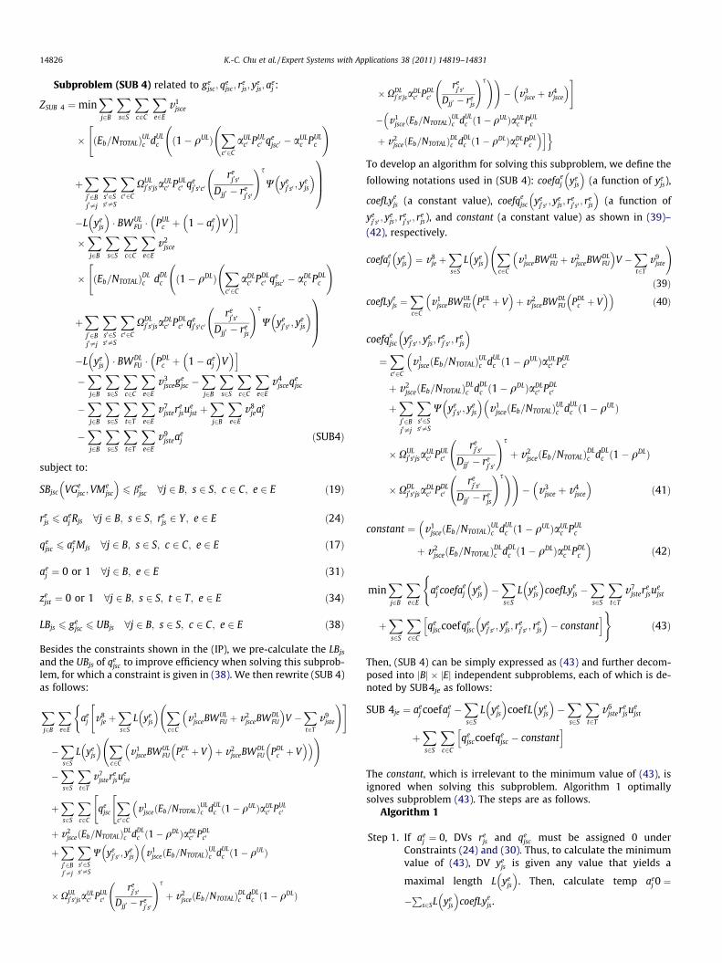
Subproblem (SUB 4) related to gejsc; q

ejsc; r

ejs; y

ejs; a

ej :

ZSUB 4 ¼minXj2B

Xs2S

Xc2C

Xe2E

v1jsce

� ðEb=NTOTALÞULc dUL

c ð1� qULÞXc02C

aULc0 PUL

c0 qejsc0 � aUL

c PULc

! "

þXj02Bj0–j

Xs02Ss0–S

Xc02C

XULj0s0jsa

ULc0 PUL

c0 qej0s0c0

rej0s0

Djj0 � rej0s0

!s

W yej0s0 ; y

ejs

� �1CCA�L ye

js

� �� BWUL

FU � PULc þ 1� ae

j

� �V

� �i�Xj2B

Xs2S

Xc2C

Xe2E

v2jsce

� ðEb=NTOTALÞDLc dDL

c ð1� qDLÞXc02C

aDLc0 PDL

c0 qejsc0 � aDL

c PDLc

! "

þXj02Bj0–j

Xs02Ss0–S

Xc02C

XDLj0s0jsa

DLc0 PDL

c0 qej0s0c0

rej0s0

Djj0 � rejs

!s

W yej0s0 ; y

ejs

� �1CCA�L ye

js

� �� BWDL

FU � PDLc þ 1� ae

j

� �V

� �i�Xj2B

Xs2S

Xc2C

Xe2E

v3jscege

jsc �Xj2B

Xs2S

Xc2C

Xe2E

v4jsceqe

jsc

�Xj2B

Xs2S

Xt2T

Xe2E

v7jstere

jsuejst þ

Xj2B

Xe2E

v8jeae

j

�Xj2B

Xs2S

Xt2T

Xe2E

v9jsteae

j ðSUB4Þ

subject to:

SBjsc VGejsc;VMe

jsc

� �6 be

jsc 8j 2 B; s 2 S; c 2 C; e 2 E ð19Þ

rejs 6 ae

j Rjs 8j 2 B; s 2 S; rejs 2 Y; e 2 E ð24Þ

qejsc 6 ae

j Mjs 8j 2 B; s 2 S; c 2 C; e 2 E ð17Þ

aej ¼ 0 or 1 8j 2 B; e 2 E ð31Þ

zejst ¼ 0 or 1 8j 2 B; s 2 S; t 2 T; e 2 E ð34Þ

LBjs 6 gejsc 6 UBjs 8j 2 B; s 2 S; c 2 C; e 2 E ð38Þ

Besides the constraints shown in the (IP), we pre-calculate the LBjs

and the UBjs of qejsc to improve efficiency when solving this subprob-

lem, for which a constraint is given in (38). We then rewrite (SUB 4)as follows:

Xj2B

Xe2E

aej v8

je þXs2S

L yejs

� � Xc2C

v1jsceBWUL

FU þ v2jsceBWDL

FU

� �V �

Xt2T

v9jste

!" #(

�Xs2S

L yejs

� � Xc2C

v1jsceBWUL

FU PULc þ V

� �þ v2

jsceBWDLFU PDL

c þ V� �� !

�Xs2S

Xt2T

v7jstere

jsuejst

þXs2S

Xc2C

qejsc

Xc02C

v1jsceðEb=NTOTALÞUL

c dULc ð1� qULÞaUL

c0 PULc0

�""

þ v2jsceðEb=NTOTALÞDL

c dDLc ð1� qDLÞaDL

c0 PDLc0

þXj02Bj0–j

Xs02Ss0–S

W yej0s0 ; y

ejs

� �v1

jsceðEb=NTOTALÞULc dUL

c ð1� qULÞ�

�XULj0s0 jsa

ULc0 PUL

c0

rej0s0

Djj0 � rej0s0

!s


c dDLc ð1� qDLÞ

�XDLj0s0 jsa

DLc0 PDL

c0

rej0s0

Djj0 � rejs

!s!!� v3

jsce þ v4jsce

� �#

� v1jsceðEb=NTOTALÞUL


c PULc

�þ v2

jsceðEb=NTOTALÞDLc dDL

c ð1� qDLÞaDLc PDL

c

�ioTo develop an algorithm for solving this subproblem, we define the

following notations used in (SUB 4): coefaej ye

js

� �(a function of ye

js),

coefLyejs (a constant value), coefqe

jsc yej0s0 ; y

ejs; r

ej0s0 ; r

ejs

� �(a function of

yej0s0 ; y

ejs; r

ej0s0 ; r

ejs), and constant (a constant value) as shown in (39)–

(42), respectively.

coefaej ye

js

� �¼ v8

je þXs2S

L yejs

� � Xc2C

v1jsceBWUL

FU þ v2jsceBWDL

FU

� �V �

Xt2T

v9jste

!

ð39Þ

coefLyejs ¼

Xc2C

v1jsceBWUL

FU PULc þ V

� �þ v2

jsceBWDLFU PDL

c þ V� ��

ð40Þ

coefqejsc ye

j0s0 ; yejs; r

ej0s0 ; r

ejs

� �¼Xc02C

v1jsceðEb=NTOTALÞUL


c0 PULc0

�þ v2


c ð1� qDLÞaDLc0 PDL

c0

þXj02Bj0–j

Xs02Ss0–S

W yej0s0 ; y

ejs

� �v1

jsceðEb=NTOTALÞULc

�dUL

c ð1� qULÞ

�XULj0s0 jsa

ULc0 PUL

c0

rej0s0

Djj0 � rej0s0

!s


c dDLc ð1� qDLÞ

�XDLj0s0 jsa

DLc0 PDL

c0

rej0s0

Djj0 � rejs

!s!!� v3

jsce þ v4jsce

� �ð41Þ

constant ¼ v1jsceðEb=NTOTALÞUL


c PULc

�þ v2


c ð1� qDLÞaDLc PDL

c

�ð42Þ

minXj2B

Xe2E

aej coefae

j yejs

� ��Xs2S

L yejs

� �coefLye

js �Xs2S

Xt2T

v7jstere

jsuejst

(

þXs2S

Xc2C

qejsccoefqe

jsc yej0s0 ; y

ejs; r

ej0s0 ; r

ejs

� �� constant

h i)ð43Þ

Then, (SUB 4) can be simply expressed as (43) and further decom-posed into jBj � jEj independent subproblems, each of which is de-noted by SUB4je as follows:

SUB 4je ¼ aej coefae

j �Xs2S

L yejs

� �coefL ye

js

� ��Xs2S

Xt2T

v6jstere

jsuejst

þXs2S

Xc2C

qejsccoefqe

jsc � constanth i

The constant, which is irrelevant to the minimum value of (43), isignored when solving this subproblem. Algorithm 1 optimallysolves subproblem (43). The steps are as follows.

Algorithm 1

Step 1. If aej ¼ 0, DVs re

js and qejsc must be assigned 0 under

Constraints (24) and (30). Thus, to calculate the minimumvalue of (43), DV ye

js is given any value that yields a

maximal length L yejs

� �. Then, calculate temp ae

j 0 ¼

�P

s2SL yejs

� �coefLye

js.


Step 2. If aej ¼ 1, assign a value of ye

js that gets a maximal length

L yejs

� �, and assign re

js equal to Rjs. Each subproblem SUB4je

can be further decomposed into jSj � jCj independent sub-

problems to optimally solve the coefqejsc ye

j0s0 ; yejs; r

ej0s0 ; r

ejs

� �by

repeating Steps 2.1 and 2.2 given a pair of yejs and re

js.Step 2.1 Assign LBjs, which is defined in Constraint (38) to

qejsc .

Step 2.2 Each coefqejsc exhaustively searches all combina-

tions of jBj � jSj, and gets DVs yej0s0 and re

j0s0 whenthe minimum value of coefqe

jsc is calculated.Assign the minimum value to tempmin ae

j 1Step 2.3 Update tempmin ae

j 1, if a smaller value of temp-min ae

j 1 is calculated.Step 2.4 Increase qe

jsc by one if it is less than UBjs and Con-straint (19) is satisfied, and go to Step 2.1; other-wise, end Step 2.

Step 3. Select the minimal value from jSj � jCj of tempmin aej 1, and

assign it to temp aej 1.

Step 4. In each of the jBj � jEj subproblems, compare temp aej 0

with temp aej 1, and choose the smaller one. If the smaller

one is temp aej 0, assign 0 to ae

j ; rejs and qe

jsc , and select any

one of yejs that gets a maximal length L ye

js

� �; else, if the

smaller one is temp aej 1, assign ae

j ¼ 1, and assign rejs; q

ejsc ,

and yejs to associated values.

3.3. Getting primal feasible solutions

After solving subproblems (SUB 1), (SUB 2), (SUB 3), and

(SUB 4), the objective value of ZD v1jsce;v2

jsce;v3jsce;v4

jsce;v5le;v6

jslte;�

v7jste;v8

je;v9jsteÞ is a lower bound (LB) of ZIP. Based on the problem

(LR), the dual problem ZD ¼max ZD V1jsce;v2

jsce;v3jsce;v4

jsce;v5le;v6

jslte;�

v7jste;v8

je;v9jsteÞ is constructed to calculate the tightest LB of the prob-

lem (IP), subject to v1jsce; v2

jsce;v4jsce;v5

le;v6jslte;v7

jste;v8je;v9

jste

� �P 0 and

v3jsce. Because of the complexity of an integrated comprehensive

planning model, we further propose the following primal heuris-tics to calculate an upper bound (UB): (1) a BS configuration andcall admission control (CAC) subproblem, (2) resource and capacitymanagement, and (3) a traffic routing and topology designsubproblem.

3.3.1. BS configuration and CAC subproblemsThere are two issues to be considered by this primal heuristic:

(1) cost minimization of network planning; (2) all MSs should becompletely serviced by the network. Thus, we try to serve allMSs with the smallest number of BSs with

Pj2B

Ps2Sze

jst ¼ 1, irre-spective of the antenna type (omni-directional or smart antenna)adopted. However, this raises the question: How many BSs are re-quired and where should they be placed? The answers to thesequestions depend primarily on the MS distribution. In the BS allo-cation subproblem, if

Pe2E

Ps2S

Pt2T ze

jst ¼ 0, the implication is thatinstalling BS j is unnecessary. Furthermore, each BS configurationuses an omni-directional antenna if

Pt2T ze

js1t >P

s2fs2 ;s3 ;s4gP

t2T zejst;

otherwise, it uses a smart antenna.For each BS j (written as BSj), denote maxBSj as the total number

of MSs that can be serviced by BSj, and let minBSj be the totalnumber of MSs that are only serviced by BSj. Based on both minBSj

and maxBSj, the traffic load in BSj is given by loadBSj =minBSj � jTj + maxBSj (actually jTj can be any large number). Then,all loadBSj are sorted in descending order to minimize costs. Thus,in Algorithm 2, the installation and configuration of BSs and CACfor MSs are considered jointly.

Algorithm 2

Step 1. For each network state e, calculate all loadBSj and sortthem in descending order.

Step 2. Sort the elements in set FS in ascending order of the ele-ment length.

Step 3. Build (hj = 1) and activate ðaej ¼ 1Þ BSs that cover MSs only

served by one BS.Step 3.1 Build BSj from which minBSj is nonzero. Config-

ure BSj with an omni-directional antenna(bj1 = 1), and allocate the first element in theset FS to ye

js. Activate BSj with the maximumradius of power transmission re

js if it satisfies

the QoS constraint; or deactivate BSj aej ¼ 0

� �.

Step 3.2 Repeat Step 2 until the BSs are built.Step 4. Select a BS that has not been placed yet by Step 2 in

descending order of loadBSj until loadBSj = 0.Step 4.1 Build BSj, configure it with an omni-directional

antenna (bj1 = 1), and allocate the first elementin the set FS to ye

js. Activate BSj with increasingpower transmission radius re

js to cover MSs thathave not been admitted, until the total numberminBSj in BSj are covered.

Step 4.2 In the coverage rejs, if MS t has not been admitted

yet and is covered by BSj, then admit it to BSj, i.e.,assign ze

jst ¼ 1 (where s is the sector I.D. of BSj

with an omni-antenna), if the QoS constraint issatisfied; otherwise ze

jst ¼ 0.Step 4.3 Repeat Step 3 until all BSs are checked.

Step 5. Deal with the MSs that have not been admitted, and re-home them in the nearest active BS.

Step 6. For each BSj, calculate the aggregate traffic gejsc

� �and the

required channel qejsc

� �.

Step 7. Check QoS, and repeat this step until the QoS requirementin each BSj is satisfied.Step 7.1 If MS t was previously assigned to an omni-

directional antenna (bj1 = 1), we re-assign theMS to a smart antenna (adjust bj2 = 1), and viceversa. Then, we adjust ze

jst to fit the antenna typeof each BSj.

Step 7.2 Re-assign yejs with the next element if the QoS

requirement is violated.Step 8. Adjust the power transmission radius re

js for all BSj to coverthe MS that is farthest away from each BSj.

3.3.2. Topology design, capacity management, and traffic routingsubproblems

The backbone topology design is by nature a minimum costspanning tree problem. As shown in Fig. 5, the traffic on link L2is aggregated by link L3 from several BSs that are jointly connectedto a specific MSC node. Furthermore, to model the node constraint,we add an auxiliary link, L1, with weight zero. To fulfill the nodesplitting requirement. Irrespective of whether the link or the nodeconstraints are considered, they are expressed jointly in Constraint(17). The steps of the primal Algorithm 3 for solving this subprob-lem are as follows:

Algorithm 3

Step 1. For each network state e, define a link weight. Applyingthe minimum spanning tree algorithm to solve this sub-problem, each

Pe2Ev5

le means a specific link and its lengthis the weight cost (actually the link cost is a function of thelink length).

Step 2. Check the aggregate traffic and capacity.


Step 2.1 For each link L3, calculate the aggregate trafficf elc

� �generated by all OD pairs.

Step 2.2 Properly assign the transmission capacity nelc

� �,

subject to the pre-defined call blocking probabil-ity threshold in (20).

Step 3. Construct a minimum cost spanning tree.Step 3.1 Calculate the aggregate traffic on link L2, where

the traffic is aggregated by link L3 from severalBSs that are jointly connected to a specific MSCnode.

Step 3.2 Construct a minimum cost spanning tree subjectto the pre-defined capacity constraint in (17).

(a) Given A(d)=1.5 Erlangs

3.5E+07

3.7E+07

3.9E+07

4.1E+07

4.3E+07

4.5E+07

4.7E+07

4.9E+07

5.1E+07

5.3E+07

10 20 30 40 50 60 |T|

A(v)=0.1A(v)=0.2A(v)=0.3A(v)=0.4A(v)=0.5

ZIP

3.

3.

3.

4.

4.

4.

4.

4.

5.

5.

Fig. 6. Planning costs as a function of jTj w

0

5

10

15

20

25

30

35

40

10 20 30 40 50 60 |T|

Gap

(%)

A(v)=0.1A(v)=0.2A(v)=0.3A(v)=0.4A(v)=0.5

(a) Error gap

Fig. 7. Performance analysis of the network p

(a) Total cost

2.E+07

3.E+07

4.E+07

5.E+07

6.E+07

7.E+07

8.E+07

9.E+07

10 20 30 40 50 60 |T|

F-LRF-SAN-LRN-SA

ZIP

Fig. 8. Cost comparison of variou

Step 4. Repeat Steps 1–3 to consider all network states, each ofwhich chooses the maximum capacity for each link as aprimal solution.

4. Computational experiments

4.1. Parameters

In this work, we consider voice traffic (v) and data traffic (d),where v, d 2 C. The number of OD pairs is half the total numberof MSs(jOj = jTj/2). Each OD pair belongs to only one traffic type,either voice or data traffic, and the amount of voice-data traffic

(b) Given A(d)=3.0 Erlangs

5E+07

7E+07

9E+07

1E+07

3E+07

5E+07

7E+07

9E+07

1E+07

3E+07

10 20 30 40 50 60 |T|

ZIP

A(v)=0.1A(v)=0.2A(v)=0.3A(v)=0.4A(v)=0.5

ith respect to voice traffic intensities.

0

500

1000

1500

2000

2500

3000

10 20 30 40 50 60|T|

CPU

(sec

onds

)

A(v)=0.1A(v)=0.2A(v)=0.3A(v)=0.4A(v)=0.5

(b) CPU time

lanning model, given A(d) = 1.5 Erlangs.

0%

10%

20%

30%

40%

50%

60%

70%

10 20 30 40 50 60 |T|

Impr

ovem

ent (

%)

F-LR vs. F-SAN-LR vs. N-SA

(b) Improvement over SA

s scenarios and approaches.

0

100

200

300

400

500

600

700

800

900

1000

1 16 31 46 61 76 91 106 121 136 151 166 181 196

Iteration

Mean

V1 V2 V3'V3" V4 V5V6 V7 V8

Fig. 9. Sensitivity analysis of Lagrangean multipliers for the planning problem.


in all OD pairs is 50–50. The experiment environment is given asjBj = 15, and jKj = 2 (omni-directional antenna and three uniformsectors) introduces jSj = 4(1 + 3). The associated QoS parametersare given as elv ¼ 0:01; eld ¼ be

jsv ¼ 0:03; bejsd ¼ 0:05 (Chu & Lin,

2004, 2006), and the required bit energy to noise ratio (BENR)for voice (v) traffic and data (d) traffic is ðEb=NTOTALÞUL

v ¼ðEb=NTOTALÞDL

v =7 dB and ðEb=NTOTALÞULd ¼ ðEb=NTOTALÞDL

d =6 dB (Kim,Jeong, Jeon, & Choi, 2002) respectively. Activity factors (AFs) are gi-ven as aUL

v ¼ aDLv ¼ aUL

d ¼ aDLd ¼ 0:5 (Jeon & Jeong, 2001, 2002; Kim

et al., 2002). The unit costs are assigned as DB = 5,000,000,Dk = 100,000, and Dl = 50 per kilometer per channel. The informa-tion rates are dUL

v ¼ dDLv ¼ 9:6 kbps (Choi & Kim, 2001; Kim & Jeong,

2000; Kim et al., 2002), and dULd ¼ dDL

d ¼ 38:4 kbps (Kim & Jeong,2000); and the numbers of channels required are qv = 1 andqd = 4. The orthogonality factors are qUL = 0.5 and qDL = 0.5, andthe power is perfectly controlled by PUL

v ¼ 10 dB, PDLv ¼ 15 dB,

PULd ¼ 15 dB, and PDL

d ¼ 20 dB (Kim et al., 2002).

4.2. Results

The computational experiments focus on jBj = 10, and the plan-ning cost is a function of jTj. It is given that ul2L1

¼ 100 Erlangs, andul2fL2 ;L3g ¼ 50 Erlangs. With regard to voice traffic intensity, wesimply denote the voice intensity Av(o) and data intensity Ad(o) ofOD pair o as A(v) and A(d), respectively. For given A(d) = 1.5 andA(d) = 3.0 Erlangs, the costs are shown in Fig. 6 (a) and (b), respec-tively. The cost of A(d) = 3.0 is more than 1% higher than that ofA(d) = 1.5. Irrespective of which A(d) is given, the more A(v) isloaded, the higher will be the calculated the cost. However, irre-spective of which A(v) is given, the costs converge whenever jTjis in the largest value. The results indicate that the total numberof MSs in the system significantly affects the overall planning cost.

Given A(d) = 1.5, other measurements, namely the error gap andCPU time, are also reported, as shown in Fig. 7. Both measurementsare also expressed as a function of jTjwith respect to the voice traf-fic intensities. In Fig. 7(a), the total number of gaps is calculated inthe range 12–34%; the more intensity A(v) is given, the looser willbe the calculated gap. In contrast to a smaller value of jTj, a largerjTj has a tighter gap. With regard to the effect of jTj on the CPUtime, Fig. 7(b) shows that the CPU time is an increasing functionof the total number of MSs. Nevertheless, the traffic intensityA(v) of each MS is not a significant factor in the CPU time.

To evaluate the performance of the planning model, which issolved by the LR approach, we implement a simple algorithm(SA), and also consider two network state scenarios: one for a nor-

mal state (N), where there are no failures among BSs, and the otherfor a failure state (F), where there are failures among the BSs.Fig. 8(a) summarizes the cost comparison of the solution ap-proaches in conjunction with the states. In terms of BS failures,the total cost is 26% more than in the normal state given jTj = 10,while it is more than 45% given jTj = 60. Clearly, the proposed LRapproach outperforms the SA algorithm. In addition, the largerthe number of MSs, the more improvement there will be in the to-tal planning cost. For a failure state, the results in Fig. 8(b) showthat the improvements, denoted by F-LR vs. F-SA, are within therange 10–60% when jTj is set between 10 and 60. Meanwhile, inthe normal state, the improvements, denoted by N-LR vs. N-SA,are in the range 5–40%.

4.3. Sensitivity analysis

After solving the integrated network planning problem, we havea rough representation of a real case. From a management perspec-tive, the most important insights are gained from the analysis afterfinding a primal feasible solution for the original model. This anal-ysis is commonly called sensitivity analysis and answers questionsabout what would happen to the optimal solution if the parame-ters in the model were varied. In addition, by using the LR ap-proach to solve the model, some constraints are relaxed andmultiplied by the corresponding Lagrangean multipliers. Fromthe analysis of the multipliers, we can understand the managerialimplications of the constraints. We run the analysis up to 1000iterations, but the values of the multiplier almost converge to thecorresponding constant values after 200 iterations. Fig. 9 showsthe results up to 200 iterations. The greater the value of the multi-plier, the more important will be the corresponding constraint inthe problem. Multiplier V7 related to constraint (23) convergesto the largest value 900. This means the service requirement isthe most important issue in solving the planning problem, as anycall requests are admitted to the coverage area of a cell. The impor-tance of the service requirement stems from the decision variationof the BS installation, as well as the BS configuration. MultipliersV30 (related to the node constraint) and V300 (related to the linkconstraint) converge to 320 and 500, respectively, which impliesthat the link constraint is of more concern than the node constraintfor an MSC. Other multipliers calculate much smaller values thanthe previous three; for example, the multipliers V1 and V2 areclose to 10 or lower. Because the traffic load is unsaturated, wedo not discuss V1 and V2 here.

Fig. 10. Sensitivity analysis of the effect of the capacity constraints on the planningcost.


The proposed network planning model considers an embeddedsystem in which some of the equipment pre-exists, as well as adesert system in which all of the equipment is newly installed.The multiplier analysis indicates that the capacity constraints inthe model are significant. To further investigate the effects of theconstraints, Fig. 10 shows that ZIP is varied when the parameter(capacity threshold) is changed. Denote u1 and u2 as the thresh-olds for the node constraint and the link constraint, respectively.The link constraint affects the total cost more significantly thanthe node constraint. For the link constraint (u2), the effect onthe cost is more significant with the decreasing threshold (4.4%)than the increasing threshold (�2%).

5. Conclusion

5.1. Research contributions

Because of ever-growing user demand and advances in technol-ogy, CDMA has received increasing attention in recent years. How-ever, it is still a challenge for system planners, managers andadministrators to plan and manage such complex systems in anefficient and effective way. To address this issue, we propose anintegrated planning model for survivable CDMA networks. Themodel considers the following issues jointly: (1) wireline networkissues: topology design and link capacity management; (2) cellularnetwork issues: cell/BS planning (site selection), cell/BS coverage(power transmission radius), sectorization (BS configuration), andsurvivability; and (3) CDMA issues: uplink/downlink SIR analysis,voice/data traffic, and bandwidth allocation (the hybrid F/CDMAscheme).

We highlight the following findings. With an increasing trafficload, more expenditure is required to provide sound service, sub-ject to a pre-defined capacity constraint. The proposed modeland solution approach yield a better solution quality as the systemload increases. With regard to the computational results, the costof providing network survivability in the planning stage is 45%more than that of non-survivability. The proposed LR approachoutperforms the SA algorithm, with a cost improvement of 60%.In addition, the link constraint is more important to the total costthan the node constraint. Given a link constraint, the cost is af-fected more significantly by a decreasing threshold than by anincreasing threshold. Thus, the threshold value should be setappropriately. If the right hand-sides (thresholds) of the capacityconstraints for both nodes and links are given very large values,the proposed planning model also uses such values for a desert sce-nario. In other words, the nodes as well as the links can be assignedas much capacity as necessary after the planning stage. Generallyspeaking, the model directs network planning as well as capacity

management to meet the requirements of CDMA-based 3Gsystems.

5.2. Managerial implications

Network planning is a complex task that has to meet many sys-tem requirements. A quite common requirement is the necessity totrade off all design objectives against one another, while respectingtheir individual importance. The solution to the planning problemrequires a large number of algorithms, each of which focuses on aproblem with specific constraints. When the survivability issue isconsidered in the planning stage, the cost is lower than that ofdeploying redundant equipment in each BS. We also considercapacity management in links and nodes. The proposed model isnot only a valuable reference for network planning in a new field(desert scenarios), but also fits the planning requirements whensome equipment pre-exists (embedded scenarios). This is becausewe give a constant value to several decision variables, so the modelis adaptable to various scenarios. We consider link and node con-straints that fit the requirements for embedded systems. Withincreasing traffic, the planning costs are higher, which indicatesthat capacity needs to be expanded to meet the scenario of con-stantly increasing traffic. It is noteworthy that the proposed modelprovides survivability in the network planning stage. With regardto capacity management, the link constraint affects the total plan-ning cost more significantly than the node constraint. Thus, cellplanning that addresses MS coverage as well as topological designplays an important role in an integrated network planningproblem.

Acknowledgement

This paper received Dragon Thesis Award, Gold Medal, AcerFoundation, 2005.

References

Ali, S. Z. (2002). An efficient branch and cut algorithm for minimization of numberof base stations in mobile radio networks. In Proceedings of IEEE PIMRC (Vol. 5,pp. 2170–2174).

Amaldi, E., Capone, A., & Malucelli, F. (2003). Planning UMTS base station location:Optimization models with power control and algorithms. IEEE Transactions onWireless Communications, 2(5), 939–952.

Binzer, T., & Landstorfer, F. M. (2000). Radio network planning with neuralnetworks. In Proceedings of IEEE VTC-Fall (Vol. 2, pp. 811–817).

Bose, R. (2001). A smart technique for determining base-station locations in anurban environment. IEEE Transactions on Vehicular Technology, 50(1), 43–47.

Castañeda-Camacho, J., Uc-Rios, C. E., & Lara-Rodríguez, D. (2003). Reverse linkErlang capacity of multiclass CDMA cellular system considering nonidealantenna sectorization. IEEE Transactions on Vehicular Technology, 52(6),1476–1488.

Choi, W., & Kim, J. Y. (2001). Forward-link capacity of a DS-CDMA system withmixed multirate sources. IEEE Transactions on Vehicular Technology, 50(3),737–749.

Chu, K. C., Hung, L. P., & Lin, F. Y. S. (2009). Adaptive channel reservation for calladmission control to support prioritized soft handoff calls in a cellular CDMAsystem. Annals of Telecommunications, 64(11–12), 777–791.

Chu, K. C., & Lin, F. Y. S. (2004). Network planning and capacity managementconsidering adaptive sectorization in survivable FDMA–CDMA systems. InProceedings of IEEE APCCAS (pp. 465–468).

Chu, K. C., & Lin, F. Y. S. (2006). Survivability and performance optimization ofmobile wireless communication networks in the event of base station failure.Computers and Electrical Engineering, 32(1–3), 50–64.

Chu, K. C., Lin, F. Y. S., & Wang, C. S. (2010). Modeling of adaptive load balancingwith hybrid FCDMA and sectorization schemes in mobile communicationnetworks. Journal of Network and Systems Management, 18(4), 395–417.

Chu, K. C., Wang, C.-S., & Lin, F. Y. S. (2010). An admission control-based benefitoptimization model for mobile communications: the effect of a decision timebudget. Journal of Network and Systems Management, 18(2), 169–189.

Chuprun, S., & Bergstrom, C. S. (1998). Comparison of FH/CDMA and DS/CDMA forwireless survivable networks. In Proceedings of IEEE GLOBECOM (Vol. 3, pp.1823–1827).

Duque-Anton, M., Kunz, D., & Ruber, B. (1993). Channel assignment for cellularradio using simulated annealing. IEEE Transactions on Vehicular Technology,42(1), 14–21.


Eng, T., & Milstein, L. B. (1994). Comparison of hybrid FDMA/CDMA systems infrequency selective Rayleigh fading. IEEE Journal on Selected Area inCommunications, 12(5), 938–951.

Garg, N., Simha, R., & Xing, W. (2002). Algorithms for budget-constrained survivabletopology design. In Proceedings of IEEE ICC (Vol. 4, pp. 2162–2166).

Ghashghai, E., & Rardin, R. L. (2002). Using a hybrid of exact and genetic algorithmsto design survivable networks. Computers and Operations Research, 29(1), 53–66.

Hamidian, K., & Payne, J. (1997). Performance analysis of a CDMA/FDMA cellularcommunication system with cell splitting. In Proceedings of IEEE ISCC (pp. 545–550).

Hanly, S., & Mathar, R. (2002). On the optimal base-station density for CDMAcellular networks. IEEE Transactions on Communications, 50(8), 1274–1281.

Hao, Q., Soong, B.-H., Gunawan, E., Ong, J.-T., Soh, C.-B., & Li, Z. (1997). A low-costcellular mobile communication system: A hierarchical optimization networkresource planning approach. IEEE Journal on Selected Areas in Communications,15(7), 1315–1326.

Huang, X., Behr, U., & Wiesbeck, W. (2000). Automatic base station placement anddimensioning for mobile network planning. In Proceedings of IEEE VTC-Fall (Vol.4, pp. 1544–1549).

Hurley, S. (2002). Planning effective cellular mobile radio networks. IEEETransactions on Vehicular Technology, 51(2), 243–253.

Jeon, W. S., & Jeong, D. G. (2001). Call admission control for mobile multimediacommunications with traffic asymmetry between uplink and downlink. IEEETransactions on Vehicular Technology, 50(1), 59–66.

Jeon, W. S., & Jeong, D. G. (2002). Call admission control for CDMA mobilecommunications systems supporting multimedia services. IEEE Transactions onWireless Communications, 1(4), 649–659.

Kaufman, J. S. (1981). Blocking in a shared resource environment. IEEE Transactionson Communications, 29(10), 1474–1481.

Kim, W. S. & Prabhu, V. K. (1998). Enhanced capacity in CDMA systems withalternate frequency planning. In Proceedings of IEEE ICC (Vol. 2, pp. 973–978).

Kim, D., & Jeong, D. G. (2000). Capacity unbalance between uplink and downlink inspectrally overlaid narrow-band and wide-band CDMA mobile systems. IEEETransactions on Vehicular Technology, 49(4), 1086–1093.

Kim, S. W., Jeong, D. G., Jeon, W. S., & Choi, C.-H. (2002). Forward link performance ofcombined soft and hard handoff in multimedia CDMA systems. IEICETransactions on Communications, E85-B(7), 1276–1282.

Lee, C. Y., & Kang, H. G. (2000). Cell planning with capacity expansion in mobilecommunications: A tabu search approach. IEEE Transactions on VehicularTechnology, 49(5), 1678–1691.

Lee, C. Y., Kang, H. G., & Park, T. (2002). A dynamic sectorization of microcells forbalanced traffic in CDMA: Genetic algorithms approach. IEEE Transactions onVehicular Technology, 51(1), 63–72.

Liberti, J. C., & Rappaport, T. S. (1994). Analytical results for capacity improvementsin CDMA. IEEE Transactions on Vehicular Technology, 43(3), 680–690.

Medhi, D. (1994). A unified approach to network survivability for teletrafficnetworks: Models, algorithms and analysis. IEEE Transactions onCommunications, 42(2–4), 534–548.

Merchant, A., & Sengupta, B. (1995). Assignment of cells to switches in PCSnetworks. IEEE/ACM Transactions on Networking, 3(5), 521–526.

Pierre, S., & Houeto, F. (2002). A tabu search approach for assigning cells to switchesin cellular mobile networks. Computer Communications, 25(5), 464–477.

Saraydar, C. U., & Yener, A. (2001). Adaptive cell sectorization for CDMA systems.IEEE Journal on Selected Areas in Communications, 19(6), 1041–1051.

Snow, A. P., Varshney, U., & Malloy, A. D. (2000). Reliability and survivability ofwireless and mobile networks. IEEE Computer, 33(7), 49–55.

Takeo, K., Sato, S., & Ogawa, A. (1999). A base station selection technique for up/downlink in CDMA systems. In: IEEE VTC-Spring (Vol. 3, pp. 1804–1808).

Tutschku, K. (1998). Demand-based radio network planning of cellular mobilecommunication systems. In Proceedings of INFOCOM (Vol. 3, pp. 1054–1061).

Tutschku, K., & Tran-Gia, P. (1998). Spatial traffic estimation and characterizationfor mobile communication network design. IEEE Journal on Selected Areas inCommunications, 16(5), 804–811.

Wang, W., & Rushforth, C. K. (1992). An adaptive local-search algorithm for thechannel-assignment problem. IEEE Transactions on Vehicular Technology, 45(3),459–466.

Wibisono, G., & Darsilo, R. (2001). The effect of imperfect power control andsectorization on the capacity of CDMA system with variable spreading gain. InProceedings of IEEE PACRIM (Vol. 1, pp. 31–34).

Wu, J.-S., Chung, J.-K., & Sze, M.-T. (1997). Analysis of uplink and downlinkcapacities for two-tier cellular system. IEE Proceedings – Communications,144(6), 405–411.

Zhuge, L., & Li, V. O. K. (2002). Reverse-link capacity of multiband overlaid DS-CDMAsystems. Mobile Networks and Applications, 7(2), 101–113.

Zhuge, L., & Li, V. O. K. (2003). Overlaying CDMA systems with interferencedifferentials. Mobile Networks and Applications, 8(3), 269–278.

expert systems with applications -...

Documents