U.S. DEPARTMENT OF THE INTERIOR

U.S. GEOLOGICAL SURVEY

Experiments in In Situ Fish Recognition Systems Using Fish Spectral and Spatial Signatures

by

'Charles Bendall, U.S. Department of the Navy, Space and Naval Warfare Systems Center San Diego

2Steve Hiebert, U.S. Bureau of Reclamation, Denver Technical Service Center, and

2Gordon Mueller, U.S. Geological Survey, Midcontinent Ecological Science Center.

Open File Report 99-104

This report is preliminary and has not been reviewed for conformity with U.S. Geological Survey editorial standards (or with the North American Stratigraphic Code). Any use of trade, product or firm names is for descriptive purposes only and does not imply endorsement by the U.S. Government.

2 1 Electro-Optics Branch 743, San Diego, CA 92152-6241 2P.O. Box 25007 (D-8220), Denver, Colorado 80225

TABLE OF CONTENTS

Page

EXECUTIVE SUMMARY.................................................................................. iiiiINTRODUCTION................................................................................................ 1METHODS........................................................................................................... 2

Image Calibration..................................................................................... 5Calibration Error....................................................................................... 7Fish Signatures......................................................................................... 9Morphological Signatures........................................................................ 10Analysis Procedures................................................................................. 11

RESULTS and DISCUSSIONS........................................................................... 14Spectral Signatures................................................................................... 14Moments.................................................................................................. 15Moments and Morphological Signatures................................................. 18Differences Between Centers................................................................... 18Normalized Moment of Color.................................................................. 20Fourier Transform Spatial Signatures...................................................... 20Fourier Transform Signature Analysis Procedure.................................... 27Fourier Transform Signatures.................................................................... 27Histograms................................................................................................. 29Signature DataBase................................................................................... 30

CONCLUSIONS.................................................................................................... 33RECOMMENDATIONS....................................................................................... 34ACKNOWLEDGMENTS...................................................................................... 35LITERATURE CITED........................................................................................... 35APPENDIX

Supporting Figures..................................................................................... 37

TABLE Number Page

1. Summary of spectral and spatial fish signatures from Test 1 & 2.. 13

2. Summary offish identification based on spectral and spatialsignatures......................................................................................... 31

3. Summarized matrix of differentiated speciation based onspectral and/or spatial signatures..................................................... 34

FIGURE

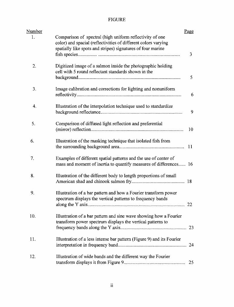
Number Page1. Comparison of spectral (high uniform reflectivity of one

color) and spacial (reflectivities of different colors varying spatially like spots and stripes) signatures of four marine fish species.................................................................................... 3

2. Digitized image of a salmon inside the photographic holding cell with 5 round reflectant standards shown in the background..................................................................................... 5

3. Image calibration and corrections for lighting and nonuniforrn reflectivity...................................................................................

4. Illustration of the interpolation technique used to standardize background reflectance.............................................................

5. Comparison of diffused light reflection and preferential(mirror) reflection............................................................................. 10

6. Illustration of the masking technique that isolated fish fromthe surrounding background area...................................................... 11

7. Examples of different spatial patterns and the use of center ofmass and moment of inertia to quantify measures of differences...... 16

8. Illustration of the different body to length proportions of smallAmerican shad and chinook salmon fry............................................ 18

9. Illustration of a bar pattern and how a Fourier transform power spectrum displays the vertical patterns to frequency bands along the Y axis................................................................................. 22

10. Illustration of a bar pattern and sine wave showing how a Fourier transform power spectrum displays the vertical patterns to frequency bands along the Y axis....................................................... 23

11. Illustration of a less intense bar pattern (Figure 9) and its Fourierinterpretation in frequency band......................................................... 24

12. Illustration of wide bands and the different way the Fouriertransform displays it from Figure 9................................................... 25

11

13. Illustration of a gradient bar pattern and how the Fouriertransform power spectrum displays that on the Y frequency axis.................................................................................................... 26

14. A Fourier transform power spectrum for striped bass...................... 29

15. Comparison of image histograms of fry and j ack chinook salmon... 30

in

EXECUTIVE SUMMARY

The objective of this study was to determine if inter-species spectral or spatial variations could be used to develop an automated fish identification system. Comparative tests were conducted using twelve fish species, (chinook salmon, striped bass, American shad, rainbow trout, northern pikeminnow, Sacramento sucker, channel catfish, hardhead, white catfish and white sturgeon) common to the Sacramento River, California. Experiments were performed under optimum laboratory conditions at the Bureau of Reclamation's Fish Research Facilities located near Red Bluff Diversion Dam, Red Bluff, California.

Spectral reflectance information was gathered from subject fish in the visible wavelengths range of 400 to 700 nm, using a CCD camera equipped with narrow band pass filters. Images were captured, digitized and stored on computer.

The twelve fish species could be divided into three broad (high, medium, and low) reflectivity categories, however, additional independent signature data was needed for in situ specific identification. Additional signatures were developed using basic morphometrics and spatial reflectivities (i.e., spots, stripes, color and reflectance gradient patterns). Morphometric measurements included fish size, pixel number within a mask, body length and depth ratios, and calculations of color moments. Spatial signatures showing promise either singly or in combination for species identification were: moment of color (quantified color gradient changes across the length or depth of the fish), center of color (quantified head and tail colors differing from the central fishes body), Fourier transformation signature of line profiles, and histogram signatures (pixel intensity- number distributions) across the entire fish.

These experiments suggest that the technology already exists for an automated, in-situ fish identification system to work under laboratory conditions. Graphic analysis of morphometrics, spectral and spatial signature curves suggested there was differentiation between 10 of the 12 species (84%). The two not discernable were the northern pikeminnow and channel catfish. However, additional research may reveal signatures that could also differentiate these species.

Future spectral and spatial signature work should focus on three topics:* Application of this data base of signatures and analysis techniques to an in-situ,

field environment. Testing is needed to demonstrate the application of this technology to field conditions and determine the applicability of field generated images with high resolution laboratory images.

*More signature validation and refinements are needed with all species. Additional signatures are needed to distinguish fish species within each broad reflective category as well as confirm the category identification.

* Develop software for fish counting and identification for a computer vision system. This should include investigations of electro-optic technologies and optical water properties appropriate for an in-situ system.

mi

INTRODUCTION

Fishery managers have long searched for a method or technology that would provide rapid and accurate information regarding the movement or migrations of fish through river corridors. Hatchery released stocks can be implanted with magnetic tags that can be detected when fish pass through sensor arrays. Unfortunately, our ability to monitor and enumerate "wild" populations of migrants is extremely limited. Present technology can be used to detect fish, and in some cases identify fish size as migrants pass through confined fish weirs or ladders. However, actual speciation requires on site observers and,or photography that can be analyzed later with precise morphometric analysis. To our knowledge, no automated fish identification system currently exists that provides accurate, in-situ fish recognition information. The goal of this study was to test the feasibility and initial data collection for an optical system that is accurate, non-lethal and adaptable to an in-situ environment.

Morphometric characteristics have been used successfully as a nonlethal method of determining smoltification levels for juvenile spring chinook salmon and steelhead (Beeman et al. 1995, Hanes et al. 1995). These authors suggested spectrography might be used as a smoltification index. Morphometric characters have been used successfully to discriminate between the Gila species (Douglas et al. 1998). Video tape recordings have been used for monitoring fish passage at nearly all the Columbia and Snake River dams and computer image techniques have been developed to remove non-fish images from recorded video tape (Hatch et al. 1998)

This study is a cooperative venture of the US Geological Survey, Bureau of Reclamation, and Department of the Navy to determine if target recognition technology can be applied to fish recognition systems. Recent advances in computer processing power, data storage, camera electronics, has brought machine vision recognition systems closer to reality. Provided the resources, we feel a system could be developed and installed at an underwater diversion or impoundment structures that could notify managers in-situ of the occupance and numbers of specific fish species. Such a system could prove vital information in the management and recovery of endemic fish stocks in conjunction with water management objectives.

Our work focussed on developing a fish signature database for the purpose of species identification. A fish signature is a distinctive set of both spectral and spatial qualities which is uiquely characteristic to only one species. Experiments focused on measuring and distinguishing differences in spectral and spatial variations of major fish species found in the Sacramento and San Joaquin Rivers. Study fish were readily available from the Tracy Fish Salvage Facility (Tracy, California) and the resulting system could be tested using videos of fish passing through fish ladders at Red Bluff Diversion Dam (Red Bluff, California-RBDD). These experiments were intended to be the first step in a series designed to develop and test signature recognition techniques. This report presents preliminary results of the spectral and spatial signature determination process and the mathematical tests used to describe differences in shape and color distributions.

1

Inter-species spectral variations is one possible signature that is compatible with machine vision systems. Spectral signatures are obvious between some tropical fish species and can occur in various forms. One fish might be uniformly brighter for all colors or uniformly brighter in a particular color band (spectral signature). There can also be distinctive color patterns, such as stripes or spots, that provide another color signature type (spatial spectral signature) (Figure 1). While these are good examples, the spectral and spatial variations of Sacramento River species are much less obvious to the human eye, but, never the less are discernable.

Color and Reflectivity

The human eye is sensitive to light in the visible spectral region which includes wavelengths ranging from 400 to 700 nanometers (10'9 meters). We refer to a unique variation in wavelength reflectivity as a spectral signature. An object's color is determined by its reflectivity in this wavelength. Fish can also have distinctive reflectivities in particular spectral (color) regions. The fish in Figure 1A or IB have a high reflectivity in the red or blue spectral region. Fish with distinctive color patterns have reflectivities that vary spatially across the fish. Figure 1C and ID are two examples offish with spatial reflectivity distributions.

To measure fish color signatures, it is necessary to measure the fish's reflectivity throughout the visible spectral region. The remainder of this report discusses how these measurements were performed and the results of the analysis.

METHODS AND APPARATUS

Fish were captured from the wild and photographed to measure their spectral and spatial signatures in specialized photographic tanks. Originally 7 fish species (Chinook salmon, striped bass, American shad, rainbow trout, northern pikeminnow, Sacramento sucker, and channel catfish) were chosen for the test. Three additional species (hardhead, white catfish, and white sturgeon) were later added. Fish were obtained from the Sacramento River by screw traps and electrofishing and from the Tracy Fish Collection Facility located in the Sacramento/San Joaquin Delta.

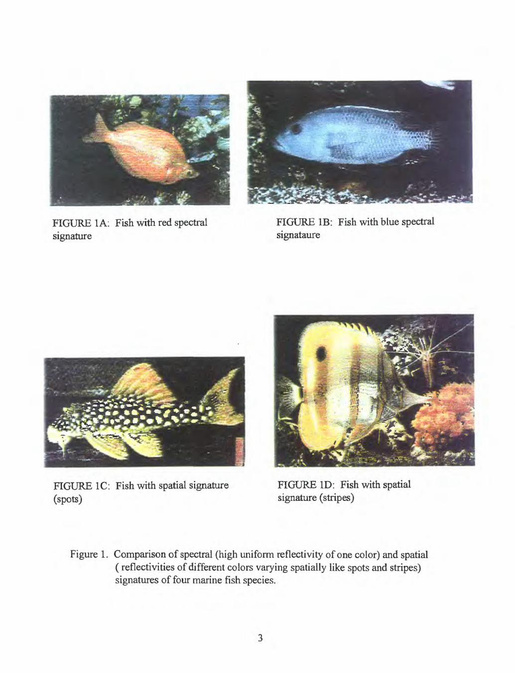
FIGURE 1 A: Fish with red spectral signature

FIGURE IB: Fish with blue spectral signataure

FIGURE 1C: Fish with spatial signature (spots)

FIGURE ID: Fish with spatial signature (stripes)

Figure 1. Comparison of spectral (high uniform reflectivity of one color) and spatial ( reflectivities of different colors varying spatially like spots and stripes) signatures of four marine fish species.

Tests were conducted in the Bureau of Reclamation's Fish Research Facility located near Red Bluff, California. Fish were brought to the facility just prior to the tests and held for a maximum of 4 days. Spectral imagery took approximately 30 to 100 minutes. At the conclusion, study fish were returned unharmed to the Sacramento River.

Test fish were placed in aO.8X1.5m diameter fiberglass tank that had a glass panel on one side. Behind the glass panel was an internal partition made of white Plexiglass that confined the fish next to the glass. The width (10-24 cm) between the glass and Plexiglas sheet could be adjusted to accommodate different sized fish while restricting their movement. A second, horizontal partition helped center the fish within the confinement. The tank was filled with clear well water and maintained at a constant 16 °C. Larger salmon and shad had to be slightly anesthetized with CO2 gas during the tests.

A charged coupled device (CCD) TV camera equipped with 16 narrow spectral bandpass filters was used to capture spectral and spatial fish signatures. The filters had center wavelengths of 400, 420, 440, 460, 480, 500, 520, 540, 560, 580, 600, 620, 640, 660, 680, and 700 nanometers (nm) (respectively the visible violet, blue, green, yellow, orange, and red spectrum). The filters had a bandpass of 15 nm except for the 700 nm filter which had a 8 nm bandpass. In addition to the narrow spectral filters, we also used broadband red, blue and green filters similar to those used in color CCD cameras. The camera was set on a tripod, perpendicular (1.5m) from the viewing chamber.

The photographic chamber was illuminated with fluorescent lights that were positioned to reduce glare. A spectral image of a fish was obtained by placing a spectral bandpass filter in front of the CCD camera lens, capturing a frame of video with a frame grabber, digitizing the image and storing the digitized image on the computer. Next, a second filter was placed in front of the lens and a second image digitized. This procedure was repeated until images were obtained with each spectral filter. At least 19 images were taken of each fish.

Figure 2 provides an example of a digitized image, showing a fish and reflectance standards. Such images were digitized into a matrix consisting of 640 x 480 elements or pixels. Each pixel was comprised of 8 bits and could have ranged between 0 and 1 depending on the intensity of light incident on the pixel. Pixels with a value of 1 are saturated (i.e., increasing the light intensity does not increase the pixel value). Saturated pixels are undesirable and we used special neutral density (ND) filters to limit the number of saturated pixels in each image.

Figure 2. Digitized image of a salmon in the photographic cell with the 5 round reflectance standards shown in the background.

Image Calibration

The camera measured the light intensity reflected from the fish within the bandpass of the filter. The intensity reflected from the fish into the camera was proportional to the product of the light intensity incident on the fish and the fish's reflectivity (Equation 1)

reflectedW- Equation 1

where IrefiectedW was the reflected intensity, IjnCjdentW was the incident intensity and was the reflectivity at wavelength X.

The term G was used to represent a number of factors that determine the amount of the reflected light that actually was imaged onto the cameras CCD array. Included in G were such factors as the size of the lens, the distance between the fish and the camera, and the transmission of the water. We have assumed that G was the same for all fish and was independent of wavelength. This is not strictly true but, simplifies the calculations. The issue of specular reflectivity that will be discussed later is an example where the assumptions regarding G are violated. The reflectivity can be determined from the ratio of the reflected and incident intensities. This task was not as easy as it might seem because the lighting was not uniform throughout the tank nor was the response of the camera uniform. In order to utilize Equation 1 it was necessary to calibrate the camera.

The first step in the calibration procedure was to correct for nonuniform lighting and the unknown factors of G. This was accomplished by placing a white background plate with uniform reflectivity in the tank. A digitized computer image of the plate, such as that shown is Figure 3 A, was obtained. The nonuniformity of the lighting and camera can be seen from the horizontal line profile shown in Figure 3B. If the camera response and lighting was uniform, the curve in Figure 3B should be a straight line. From the line profile it is evident that the combined effects of lighting, geometric factors, and camera

CALIBRATION BACKGROUND

1.5

1

0.5

00 200 400 600 NONUNIFORMITY CORRECTION

1

0.8

0.6

0.4

0.2

00

00

200 400 LINE PROFILE

600

0.5 1 PIXEL VALUE

Figure 3. Image calibration and corrections for lighting and nonuniform reflectivity

response results in a pixel values ranging from 0.1 to 1.0. The plate has a uniform reflectivity but substituting into Equation 1 without correcting for the light and camera nonuniformities would mistakenly yield nonuniform reflectance values for the plate.

The easiest way to correct for the nonuniformities was to create a correction image by replacing each pixel value in the original image by its reciprocal value (1/pixel value). Multiplication of the original image by the correction image produces a uniform response as indicated by the line profile in Figure 3C. The nonuniformity correction was valid only for the lighting and camera settings from which it was measured. It was important not to move the camera or the lights, adjust the iris on the lens or change the camera's internal gain settings while acquiring the fish images. The camera's automatic gain control was disabled and the iris fixed at the full open setting. The iris was normally used to control the intensity of the light reaching the camera's focal plane. With the iris fixed in the full open position many of the images had large numbers of saturated pixels. Neutral density filters were placed in front of the camera lens to limit the number of saturated pixels.

The next step in the calibration procedure was to convert pixel values to reflectivity. To accomplish this, a set of five reflectance standards were placed in the tank with reflectance values of 2%, 9%, 47%, 74% and 99%. The standards appeared as five circles at the top of in each digitized computer fish image. For each image, a linear least square fit was performed on the reflectance standards to provide a calibration from pixel value to reflectivity. An example of a curve is shown in Figure 3D. The horizontal axis corresponds to the pixel value (0 to 1) and the vertical axis is the corresponding reflectance values of the five standards. The straight line represents the result of the linear least square fit and gives the conversion from pixel value to reflectivity. The equation for the line show in Figure 3D is given by:

reflectivity = slope * pixel value + y intercept Equation 2

The reflectivity of each pixel was calculated by inserting the pixel value into Equation 2. Once the calibrated procedure had been completed, the spectral and spatial signatures could be extracted from the image. A new nonuniformity correction was made whenever the experimental setup was modified. This occurred whenever lights or camera were moved or lenses changed on the camera. The nonuniformity correction was assumed to be valid independent of the filter wavelength and fish. The conversion from pixel value to reflectivity was calculated for each digitized fish image.

Sources of Error in Calibration

Partially valid assumptions and systematic errors were inevitable during the calibration process and these measurements were no exception. Several of the most important are discussed below.

The frame grabber introduced a digitization offset into the data. Images acquired with the very low light levels (room darkened and the lens cap placed on the camera) did not result in pixel values of zero. Each pixel always had a small but significant value. It was necessary to remove this value before calibrating the image. For the second set of tests (Test 2-September 1995) the digitization offset was obtained from the reflection standard holder shown in Figure 2. This was painted black and had a very small reflectivity which we assumed to be zero. We located the darkest area on the holder, calculated the mean pixel value within the area and used this as the digitization offset. The digitization offset was subtracted from the image prior to calibration. In the initial tests in June, the standard holder was made of wood and did not provide a good measure of the digitization offset. Instead, we tried to locate the darkest area in the image and used the mean pixel value for this area as the digitization offset. Inaccuracies in the digitization offset would have had the greatest impact on those fish with lowest reflectivities.

For the nonuniformity correction, we had a 12 inch x 12 inch reflection standard with a reflectivity of approximately 70%. The tank cell was approximately 80-cm-wide so it required three images with the reflection standard on the left, center and right portions of the tank. The plan was to combine the images to create a uniform background. For Test 1 this process did not always produce a seamless uniform background. In these instances the Plexiglas sheet used to restrict the fish movement was used as the uniform background. The Plexiglas appeared to be uniform but, was probably not as uniform as the reflection standard. In Test 2 we unknowingly saturated a large portion of center image of the reflection standard. We again used the Plexiglas background as our uniform standard but, the calibration procedure was more complicated than in Test 1. We had fastened the five calibration standards to the Plexiglas. This produced a nonumform background where the reflection standards were located. An interpolation technique was used to approximate the Plexiglas pixel values hidden by the five reflection standards The same method was used to remove a small saturated area in the center of the Plexiglas and the horizontal fish rest. This process is illustrated in Figure 4.

The reflectance values used to convert from pixel value to reflectivity were measured in air and not water. We made several attempts to estimate their reflectivity in water but we were unable to achieve consistent results. It did appear that the ratio of reflectivities in air and water were constant. We assumed the use of the air reflectance values introduced only a scaling error.

Spatial signatures based on color moments require knowing the fish's orientation in the tank (i.e., facing left or right). Generally, the fish remained in the same orientation but on occasion reversed direction during the measurements. To speed up the analysis a single orientation was selected for each fish. Points in the spatial signature curves showing large variations could result from an incorrect orientation. This type of error was easily corrected but time consuming. Orientation errors of this type did not seem to affect the spatial signature analysis and were not corrected at this time.

ORIGINAL IMAGE USED FOR NON teOIRIyfry CORRECTIONS

Figure 4. Illustration of the interpolation technique used to standardize background reflectance.

The G term contains a number of factors that were assumed to be independent offish species. Figure 5 illustrates an important situation in which this assumption was violated. Figure 5 shows a digitized image of a striped bass. Also shown is a horizontal line profile through the fish and through the reflection standards. There are points on the fish line profile that exceed the value of the highest reflection standard. Conversion of pixel value into reflectivity produced values exceeding one. Reflectivity values cannot be greater than one. This is not an error in our calibration procedure, but results from a difference in G between the fish and the reflection standards. The reflection standards used in the calibration proceedure were diffuse reflectors. This means that light incident on the reflection standards was reflected in all directions and only a small portion of the light was imaged by the camera. On the other hand, the bright areas of the fish act like tiny mirrors. These areas were oriented so that the light from the fluorescence lights was reflected preferentially towards the camera, which made them appear to have a reflectivity greater than one. These unreasonably high reflectivities were not a serious problem, but do illustrate that signatures can be highly dependent on lighting geometry.

Fish Signatures

Fish signature data was obtained during two 1-week periods in June (Test 1) and September (Test 2) 1995. Table 1 lists the species and number of samples for species measured during each test. Spectral signatures often species were measured between the two tests. Furthermore, salmon and shad were split into categories, "small" and "large", for a total of 12 fish "species".

SJRIPED BASSWFH SATURATED PIXELS

Figure 5. Comparison of diffuse light reflection and preferential (mirror) reflection.

Morphological Signatures

Two very simple morphological signatures have been included in the signature data base: fish size (based on pixel count) and fish length to body depth ratio. This information was a by product of the spectral and spatial signatures calculations and the morphological signatures were included to help confirm cluster and species identification. The number of pixels comprising the fish mask was used to measure fish size. Pixel summation was a simple function for the image processing hardware and was also required for bulk reflectance calculations. This information was useful in the identification of large shad, striped bass and large chinook salmon within their respective clusters. Fish length and body depth calculations resulted from calculations of fish moments (see next section for a discussion of moments). This information provided a unique signature for white sturgeon and was also useful in confirming large salmon identifications.

Spectral signatures were obtained only for fish side views. Spectral images of 42 fish were taken during Test 1. Of these, 39 images were used to obtain spectral signatures. Nineteen images are taken of each fish yielding about 740 images analyzed in Test 1. Top and bottom view spectral images of an additional 13 fish were obtained, but were not analyzed or presented in this report. Side view images of 33 fish were taken during Test 2 and 31 fish were used in the analysis. This corresponds to a total of nearly 630 images. An additional 18 fish were also examined but, not used in the study primarily because the images were not of a side view. In the two tests, nearly 1400 images were analyzed.

10

Considering the large number of images collected during this program there were very few lost fish images. From Test 1 images of hardhead number 2 at 620 nm and hardhead number 3 at the broadband green filter are missing. From Test 2 images of catfish number 3 at 680 nm, striped bass number 2 for both the 680 nm and the broadband blue filters and the chinook number 6 at 660 nm filter are missing. The missing files had minimal impact on the conclusions of this report. The 680 nm and 700 nm data has been excluded in our analysis because of inadequate lighting at these wavelengths and the broadband data has not been processed for this report. The software was not designed to check for missing data files and in these cases the reflectivity was assumed to be 0.

Analysis Procedure

Extracting the signatures from the digitized images was not technically difficult, but it was time consuming. To analyze the fish signature it was necessary to construct a mask for each fish. Since the fish moved between images, it was necessary to construct a mask for each color image. The mask is a computer generated image of the digitized fish image. Unlike the digitized fish image, the mask only has pixel values of 1 or 0. Every pixel in the mask corresponding to a fish pixel was assigned the value 1 while all other pixels are zero. Multiplication of the digitized fish image by the mask extracts the fish from the image and removes the unwanted background. This process is illustrated in Figure 6.

(6B) FISH MASK

ROTATED FISH.pNLY

Figure 6. Illustration of the masking technique applied to each image to isolate fish from the surrounding background area.

11

Following the image calibration procedure, fish images were multiplied by the mask to extract the fish and the spectral and spatial signatures. Several types of spatial signatures were evaluated for potential species identification. Most proved unsatisfactory but five signatures were selected as the most promising candidates. These five are described in greater detail later. This yielded a total of six types of signatures (five spatial and one spectral).

During Test 2 multiple images were often recorded at each filter wavelength. The images differed in the amount of neutral density (ND) filtering utilized. This was done to examine the effects of pixel saturation on the signatures. It was necessary to develop a decision criteria that could be used to select one image for the signature measurements. Three criteria were tested: the image with highest reflectivity, the image with best fit between pixel value and reflectivity (Figure 3D) and the image with smallest number of saturated pixels. Fortunately, all three criteria generally selected the same image and the highest reflectivity criteria was arbitrarily used as the decision criteria.

The signatures for each species were collected into a rectangular matrix with 19 columns. Each column corresponded to one of the 19 bandpass filters used in the study. The number of rows in the matrix corresponded to the number offish measured for that species. Separate signature matrices were obtained for the spectral signature and four of the five spatial signatures. The Fourier transformed spatial signature, which will be explained in greater detail, was treated in a slightly different manner. The fish from Test 1 and Test 2 were also treated separately to avoid differences that could result from seasonal changes in fish coloration or slight differences in experimental procedures between the two tests. Average signatures were obtained by performing a column average on the signature matrices yielding the mean value for each bandpass filter. The standard deviation for each column was also calculated.

The spectral signature of a single fish was defined to be its average reflectivity which was calculated in the following manner: Multiplying the mask and the calibrated digital fish image extracted the fish from the background by setting all the non-fish pixels to 0. The fish pixels retained their calibrated value. A summation over all the pixels yielded a value related to the total signal reflected by the fish. A summation over all the pixels in the mask was performed which yielded the total number of pixels comprising the fish. The ratio of the total signal to the total number of pixels was the average reflectivity.

12

Table 1. Summary of spectral and spacial fish signatures of tests 1 and 2 (different trips).

Testl

1

2

3

4

5

6

7

8

9

10

Test 2

12

3

4

5

6

7

8

9

10

SPECIES

Small Chinook

Small American Shad

Large American Shad

Striped Bass

Rainbow Trout

Channel Catfish

White Catfish

Northern Pikeminnow

Hardhead

Sacramento Sucker

Small ChinookSmall American Shad

Striped Bass

Channel Catfish

White Catfish

White Sturgeon

Northern Pikeminnow

Hardhead

Sacramento Sucker

Chinook, Jack

DATA CODES

cs

shs

shl

sb

rb

cf

we

sq

hh

su

chfsh

sb

cf

we

sr

sq

hh

su

chj

SAMPLE NUMBER

4

2

2

7

3

3

1

7

7

8

2

3

3

3

2

2

4

2

4

8

COMMENTS

data contains only one sample at this time

only six have been used

two very small hardheads not used in spatial signature analysis

only seven have been used

one not used because of uncertain identification

one NP was eliminated because it had an abnormally high reflective.

13

RESULTS AND DISCUSSIONS

Spectral Signatures

The results of the spectral signature analysis indicated that fish could be grouped into three reflectance clusters. These clusters were labeled high, medium, and low. The high reflectance cluster consisted of the adult shad, shad fry, chinook salmon fry, and striped bass. The white catfish, channel catfish, white sturgeon, rainbow trout, and northern pikeminnow made up the medium reflectance cluster. The hardhead, Sacramento sucker and jack chinook salmon constituted the low reflectance cluster. The three spectral signature clusters for both tests were plotted and are shown on Figures Rl through R6 (Appendix). For each fish species there were three curves. The central curve was the average reflectance value for each wavelength. The upper and lower curves were the average value plus or minus the standard deviation at each wavelength. The region bounded by the upper and lower curves provided an indication of the range of possible reflectance values for each species. The presentation of Figures Rl through R6 shows there was considerable overlap between some species reflectivities. From that graphic analysis we concluded that, within a cluster, reflectivity was not a definitive signature.

The overlap between the high and medium and medium and low clusters are shown in Figures R7 through R14. The high and medium clusters from Test 2 (Figures R2 and R4) have been plotted together in Figure R9. The high cluster information has been plotted in red and the medium cluster in blue. The solid curves are the average species reflectivity curves and the asterisks represent the average value plus or minus the standard deviation. As can be seen from Figure R9, there is very little overlap of the blue and red curves. The average curves are well separated and the vast majority of red asterisks lie above the blue asterisks. The same information was plotted in a different manner in Figure RIO. The high cluster was plotted as a single red bar, where each bar corresponds to a separate bandpass filter. The upper and lower bounds of each bar was determined by the maximum and minimum red asterisks from Figure R9. The medium cluster data is plotted as blue bars. Areas where the red and blue bars intersect are indicated by shades of red or blue depending on amount of overlap between the high or medium clusters. In most cases the bars are completely separated. Similar plots for Test 1 are shown in Figures R7 and R8. There was slightly more overlap, but the clusters were in general well defined especially at the smaller wavelengths.

The overlap between the medium and low clusters is shown in Figures Rl 1 through R14. The medium cluster is shown in blue and the low cluster in green. Referring to Figure Rl 1 or R12, the separation between Test 1 medium and low clusters is not as great as between the high and medium clusters but still well defined. In Test 2 (Figure R13 and R14) two clusters are still evident but there was considerable overlap.

14

Spectral signatures could be used to associate a fish species with a reflectance cluster. This was especially true for species within the high reflectance cluster. There was a greater overlap between the medium and low clusters, but the separate clusters were still evident. Association of a fish with a reflectance cluster greatly reduced the task of species identification through a reduction in the number of probable species. No species tested exhibited a distinctive spectral signature that would provide a unique identification. There was a general increase in reflectivity at the longer wavelengths (reds), especially in Test 2. It was unclear if this was evidence of a seasonal variation or a systematic error in our analysis procedure.

While average reflectivity provided a good estimate of the fishes reflectance cluster, it did not yield a unique species identification. Additional signatures were still needed to distinguish fish species within each cluster as well as confirm the cluster identification. Spatial signatures in conjunction with a few simple and basic morphological signatures may provide the additional information need to provide a unique species identification.

Moments

Fish with the same average reflectivity may have different spatial color distributions. This point is illustrated in Figure 7 which shows four similar rectangles with the same average reflectivity but with different spatial color distributions. Moments are a standard technique in shape analysis and provides a quantitative measurement of differences in spatial color distributions. We found with fish, it could be used to determine color differences from the dorsal to ventral and/or head to tail changes. The formal mathematical definition for the moments of an arbitrary object appear to be quite involved but in reality the first few moments are quite intuitive. The formal expression for moments my is given in Equation 3 where the summations are over all the pixels in the X and Y directions and p(X,Y) is the pixel value at coordinate (X,Y). The X and Y directions correspond to the standard Cartesian graph coordinates (horizontal and vertical axes).

m ij = EExj * yj * p(x,y) Equation 3

The zeroth order moment (m00) is just a summation of all the pixels comprising the object. In our case, if the object is the fish, then the m0;0 is just the total signal from

15

signal = 3870 x center of mass = 11 ycenterQfrrpss=5C

s;xmQmeitofinerfja = y moment of inertia =

FIGURE 7C

signal = 3870 x center of mass=95 y center of mass = 50 x moment of inertia-3201042 y moment of inertia 838480

signal =3870x center of mass = 100y center of mass = 54x moment of inertia=3289086y moment of inertia = 777422

FIGURE 7D

signal = 3870 x center of mass=100 y tenter of mass = 50 xjmoment of inertia-39B1240 y moment of inertia = 1069080

Figure 7. Simple examples of different spatial patterns and the use of center of mass and moment of inertia to quantify measures of differences.

16

the fish. If the object is the fish mask then mo 0 is just the total number of pixels comprising the fish. The ratio of the m00 for the fish to m00 for the mask is the average reflectivity. The ratio of first order moments to the zeroth moment (Xc = m, 0/m0 0) and (Yc = m0 /moo) are the center of mass in the X and Y directions. The second moments (m2 o, m lfl and m0 2), which are the highest moment we will be concerned with, are more commonly know as the moments of inertia. The value of the moments depend on the choice of coordinate system. Interpretation of the moments is simplified if the center of mass is chosen as the origin of the coordinate system. The central moments are given by a simple modification to Equation 4.

Mu = ZZ(X - xc)' * (y - Yi)1 * P (x,y) Equation 4

A further simplification is possible if spatial signatures are determined in terms of the principal central moments. The principal central moments are calculated from Equation 4 after the object has been rotated through an angle (q) given by

tan(2*q) = 2*Mu/( M2/M0?2) Equation 5

The rotation aligns the principal axes with the X and Y axes. This rotation was important because the principal axes tend to correspond to the axes of symmetry of the fish as perceived by human observers.

Zero through second order moments were calculated for both the fish and the fish mask. Moments calculated for the mask are referred by as mass moments (i.e., center of mass or moment of inertia). Moments calculated for the fish are referred to as color moments (i.e., center of color or moment of color). Color principal moments calculate from Equation 4 after rotation through the angle given by Equation 5 were written as CP (i.e., CP0 o or CP, 0). Mass principal moments were written as MP. Several spatial signatures were calculated from combinations of these moments. Two signatures showed potential as a means of distinguishing fish within a reflectance cluster. These are referred to as (1) Difference Between Centers of Color and Mass and (2) Normalized Moment of Color.

The Difference Between Centers of Color and Mass (DBCCM) is the X (or Y) difference between the center of color and the center of mass divided by the length (or body depth) of the fish.

DBCCMx = (CP l5o - MP 1>0)/length Equation 6

or

DBCCMy = (CP0,, - MP0;1 )/width

The length or body depth normalization allow comparison offish of different sizes.

17

The Normalized Moment of Color (NMC) is the X (or Y) fish moment of color divided by the product of the total fish signal and the X (or Y) moment of inertia.

NMCx = CP2,o/(CP0,o* MP2 , 0) Equation 7

or

NMCy = CP0y(CP0>o*MPof2)

The moment of color was normalized in this manner to remove dependencies on fish size and reflectivity.

Moment and Morphological Signatures

Size

Fish size information is shown in Figures SZ1 through SZ6. The total number of pixels has been used is a measure offish size and corresponded to the MP0 0 moment of the mask. The pixel number clearly distinguishes large American shad and striped bass from small American shad and chinook salmon fry. Pixel size was also useful in distinguishing large chinook salmon from other fish in both the medium and low reflectivity clusters (Figure SZ6). Size varies throughout the life cycle of the fish and clearly fish size should be used with caution for the purposes of species identification.

Length to depth Ratio

White sturgeon have a significantly larger length to depth ratio than other species measured (Figures LWI through LW6). Length to width ratio also appeared to be a good signature for distinguishing jack chinook salmon from other fish in the low reflectance cluster. The small size of shad and salmon fry made it difficult to construct an accurate mask for these fish. Consequently, the length to depth ratio curves (Figures LWI and LW2) were ambiguous. However, a comparison of the shad and salmon fry in Figure 8 shows that shad and salmon fry of similar lengths have different body depths.

Difference Between Centers of Color and Mass (DBCCM)

The Difference Between Centers of Color and Mass (DBCCM) is the X (or Y) difference between the center of color and the center of mass divided by the length (or width) of the fish.

DBCCMx = (CP 1>0 - MP 1;0)/length Equation 8 or

DBCCMy = (CP0,i - MP0.i)/width

18

Figure 8. Illustration of the different body to length ratios of small American shad and chinook salmon fry.

This spatial signature was motivated by our need to distinguish color distribution like those used in Figure 7A, B and C. All three figures have the same signal (average reflectivity) but very different spatial distributions. Figures 7A and B can be distinguished by the value of the Y center of mass, while Figures 7 A and C can be distinguished by the X center of mass value.

Figures 7A, B and C can be compared rather easily because the rectangles are placed at the same location. Comparison of fish images was more due to fish movement. This problem was partially solved by computing the difference between the shift in center color and center of mass of each image. The X component of the DBCCM indicated if the head or tail of the fish was brighter or darker while the Y component provided equivalent information on the dorsal and ventral color distribution. A positive X component indicated that the tail was brighter than the head while a positive Y component indicated that the ventral area was brighter than the dorsal area. The length or depth normalization allowed comparison of different sized fish.

The X component (Figures DX1 through DX6) does not appear to be a useful signature. The curves all tend to overlap and contain both positive and negative values. The figures have been included for completeness. The Y component may contain some useful information. A comparison of Figures DY3 (Test 1) and DY4 (Test 2) showed there was no overlap of pikeminnow with either rainbow trout or sturgeon. White sturgeon and rainbow trout did overlap. This signature should be used with caution. Rainbow trout and white sturgeon were only available during Test 2 and there were a number of cases where promising signatures were not consistent between tests. An example was the comparison of the X Normalized Moment of Color for hardhead and sucker between Tests 1 and 2 (Figures DX5 and DX6).

19

Normalized Moment of Color (NMC)

The Normalized Moment of Color (NMC) is the X (or Y) fish moment of color divided by the product of the total fish signal and the X (or Y) moment of inertia.

NMCx = CP2 0/(CP0,o* MP2 0) Equation 9

= CP0,2/(CP0/MP0>2)or

The moment of color was normalized in this manner to remove dependencies of fish size and reflectivity. Our use of this signature was motivated by the differences between Figure 7A and D. The figures were clearly different but have the same center of mass coordinates. The two color distributions were easily distinguished by comparing moments of inertia instead of centers of mass. The X and Y normalized moments of color are shown in Figures MX1 through MX6 and MY1 through MY6. The X and Y normalized moments of color were similar, so only the X component will be discussed.

The NMC of striped bass and large American shad were normally lower (<1.1) than values for juvenile shad and salmon (Figure MX2). The standard deviation for salmon in Test 1 (Figure MX1) was large and did overlap with striped bass slightly. The large standard deviation was due to the difficulty in constructing an accurate mask for small fish. Note that there was almost a complete separation of the y component (Figure MY1). NMC for small shad and small salmon were generally greater (10~4) than for other fish species (7x10~5) studied in this project. The upper limit of the standard deviation of white catfish in Test 2 (MX4) did approach 10~4 . The NMC for jack salmon (Figure MX6) was much lower than other species in the medium and low clusters (<1.8xlO~5) with the exception of the lower standard deviation line of hardhead in Test 2.

Fourier Transform Spatial Signatures

The Fourier transformation is a well known technique for analyzing the frequency content of temporal and spatial signals. The Fourier transform expresses a complex function as a sum of simple sinusoids. This transformation often results in a more simple representation of the complex function. The following are a few examples illustrating how Fourier transforms were used to obtain fish signatures. Fourier transforms can have both real and imaginary components. It is often more useful to plot the power spectrum of the Fourier transform rather than its real or imaginary components. Figure 9 shows a pattern of 8 alternating bright and dark bars. Also shown is a horizontal line profile of the bar pattern. The bright bars have a value of 1 and the dark bars have a value of 0 as can be seen from the line profile. If this bar pattern was a fish, then the bright bars would have a very high reflectivity and the dark bars would have a reflectivity of zero. The Fourier transform power spectrum of the line profile was plotted at the bottom of Figure 9.

20

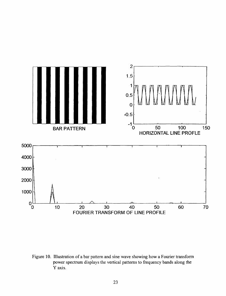
Several peaks in specific frequency bands were evident. The first occured at zero cycles and corresponded to the total signal in the pattern. If we make an analogy between the bar pattern and a fish, then the signal at zero cycles is related to the reflectivity of the fish. The second peak occurs at 8 cycles and is produced by the 8 bar pattern. The three smaller peaks at 24, 40 and 56 cycles are harmonics of the second peak at 8 and are due to the sharp edges of the bar pattern. Edge effects are illustrated in Figure 10. The bar pattern in Figure 9 is duplicated in Figure 10. The line profile of the bar pattern is shown in red. Also shown in blue is a line profile of an 8 cycle sine wave. The corresponding Fourier transform power spectrums are shown in red and blue at the bottom of Figure 10. The red power spectrum line corresponding to the line profile of the bar pattern shows the peaks at 8, 24, 40 and 56 cycles. The blue power spectrum line corresponding to the sine wave has only the peak at 8 cycles.

A second bar pattern is plotted in Figure 11 along with the corresponding line profile and Fourier transform power spectrum. The bar pattern again has a frequency of 8 cycles, but in this case the dark bars have a value of 0.5. Two differences can be seen between the Fourier transforms power spectra in Figures 9 and 11. The signal at zero frequency is greater in Figure 11. If we again make an analogy with a fish then the reflectivity of the fish in Figure 11 is greater than that in Figure 9 which is true because the dark bars in Figure 9 have zero reflectivity. Conversely the signal at 8 cycles is greater in Figure 9 indicating a greater contrast in the bar pattern. The higher harmonics are less obvious in Figure 11

Figure 12 shows a third bar pattern similar to Figure 9 except that there are four bars instead of eight. The line profiles and corresponding Fourier transform power spectrum are also shown. As expected a signal peak occurs at four cycles instead of at eight. Higher harmonics are also visible. Finally a fourth bar pattern, line profile and Fourier transform power spectrum are illustrated in Figure 13. The bar pattern is created by adding the bar patterns in Figures 9 and 12. The evidence of bars occurring at both 4 and 8 cycles is clearly seen in the accompanying power spectrum.

These figures hopefully illustrate the significance of Fourier transforms and ability to detect somewhat subtle differences. Fourier transforms provide information on a signal's frequency content. This includes information on the net strength of the signal and the strength of each frequency component of the signal

21

0

BAR PATTERN-1

0 50 100 150 HORIZONTAL LINE PROFLE

5000

4000

3000

2000

1000

00 10 20 30 40 SO'

FOURIER TRANSFORM OF LINE PROFILE60 70

Figure 9. Illustration of a bar pattern and how a Fourier transform power spectrum displays the vertical patterns to frequency bands along the Y axis.

22

BAR PATTERN

2

1.5

1

0.5

0

-0.5

-10 50 100 150

HORIZONTAL LINE PROFLE

5000

4000

3000

2000

1000

00 10 20 30 40 50

FOURIER TRANSFORM OF LINE PROFILE60 70

Figure 10. Illustration of a bar pattern and sine wave showing how a Fourier transform power spectrum displays the vertical patterns to frequency bands along the Y axis.

23

10000

8000

60001

4000

2000

0

BAR PATTERN

0

-1

IMAMM

0 50 100 150 HORIZONTAL LINE PROFLE

0 10 20 30 40 50 60 FOURIER TRANSFORM OF LINE PROFILE

70

Figure 11. Illustration of a less intense bar pattern (Figure 9) and its Fourier interpretation in frequency band.

24

BAR PATTERN

0

-10 50' 100 150

HORIZONTAL LINE PROFLE

5000

4000

3000

2000

1000

00 10 20 30 40 50

FOURIER TRANSFORM OF LINE PROFILE60 70

Figure 12. Illustration of wide bands and the different way the Fourier transform power spectrum displays it from Figure 9.

25

BAR PATTERN

0

-10 50 100 150

HORIZONTAL LINE PROFLE

5000

40001

30001

2000

1000

0 A A. .o 10 20 30 40 50

FOURIER TRANSFORM OF LINE PROFILE60 70

Figure 13. Illustration of a gradient bar pattern and how the Fourier transform power spectrum displays that on the Y frequency axis.

26

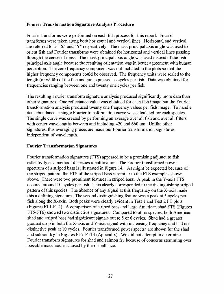
Fourier Transformation Signature Analysis Procedure

Fourier transforms were performed on each fish process for this report. Fourier transforms were taken along both horizontal and vertical lines. Horizontal and vertical are referred to as "X" and "Y" respectively. The mask principal axis angle was used to orient fish and Fourier transforms were obtained for horizontal and vertical lines passing through the center of mass. The mask principal axis angle was used instead of the fish principal axis angle because the resulting orientation was in better agreement with human perception. The zero frequency component was not included in the plots so that the higher frequency components could be observed. The frequency units were scaled to the length (or width) of the fish and are expressed as cycles per fish. Data was obtained for frequencies ranging between one and twenty one cycles per fish.

The resulting Fourier transform signature analysis produced significantly more data than other signatures. One reflectance value was obtained for each fish image but the Fourier transformation analysis produced twenty one frequency values per fish image. To handle data abundance, a single Fourier transformation curve was calculated for each species. The single curve was created by performing an average over all fish and over all filters with center wavelengths between and including 420 and 660 um. Unlike other signatures, this averaging procedure made our Fourier transformation signatures independent of wavelength.

Fourier Transformation Signatures

Fourier transformation signatures (FTS) appeared to be a promising adjunct to fish reflectivity as a method of species identification. The Fourier transformed power spectrum of a striped bass is illustrated in Figure 14. As might be expected because of the striped pattern, the FTS of the striped bass is similar to the FTS examples shown above. There were two prominent features in striped bass. A peak in the Y-axis FTS occured around 10 cycles per fish. This clearly corresponded to the distinguishing striped pattern of this species. The absence of any signal at this frequency on the X-axis made this a defining signature. The second distinguishing feature was a peak at 5 cycles per fish along the X-axis. Both peaks were clearly evident in Test 1 and Test 2 FT plots (Figures FT1-FT4). A comparison of striped bass and large American shad FTS (Figures FT5-FT6) showed two distinctive signatures. Compared to other species, both American shad and striped bass had significant signals out to 5 or 6 cycles. Shad had a greater gradual drop in both the X-axis and Y-axis signal with increasing frequency and had no distinctive peak at 10 cycles. Fourier transformed power spectra are shown for the shad and salmon fry in Figures FT7-FT14 (Appendix). We did not attempt to determine Fourier transform signatures for shad and salmon fry because of concerns stemming over possible inaccuracies caused by their small size.

27

STRIPED BASS FOURIER TRANSFORM POWER SPECTRA0.03

0.02-

0.01 -]

00 5 10 15 20

POWER SPECTRUM FOR X-AXIS (FISH LENGTH)25

5 10 15 20 POWER SPECTRUM FOR Y-AXIS (FISH WIDTH)

25

Figure 14. A Fourier transform power spectrum for striped bass

28

Previous hardhead and Sacramento sucker signatures were quite similar; however, their FTS might offer a distinctive signature. The sucker's Y-axis FTS (Figures FT31-FT34) appeared to dominate low frequencies in the range of one to four cycles.

Hardhead FTS (Figures FT35-FT38) was dominated by the Y-axis FTS at one cycle but the X-axis FTS was generally stronger at frequencies between two and four cycles. Jack chinook (Figure FT39 and FT40) X-axis FTS dominated frequencies above three cycles where there were features at both five and ten cycles. These features are distinguishable from striped bass because they are weaker and dominates the X-axis FTS rather than the Y-axis FTS. Jack chinook signatures were only measured in Test 2 and additional measurements are recommended to confirm the five and ten cycle features. Hard head, suckers and jack chinooks have much less signal throughout the frequency spectrum than the striped bass and large shad.

With the exception of rainbow trout, the FTS for species in the medium reflectance band were not distinctive and were similar to the FTS of the suckers (dominated at low frequencies by the Y-axis). The strength of rainbow trout FTS between 4 and 6 cycles was similar to that of the large shad except that the X-axis component dominates (Figure FT19 and 20). The strength of the low frequency FTS of pikeminnow, rainbow and channel catfish were greater than those by white catfish, sturgeon, sucker and hardhead. There can be a factor of two variations in the low frequency signal strength from Test 1 to Test 2, so caution should be used in deciding how much confidence to place in signatures based on the low frequency FTS strength. The FTS of the white catfish from Test 1 appears to have significant features at the higher frequencies (Figure FT25 and 26). This is because the low frequency FTS strength is significantly lower and the strength at the higher frequencies is really comparable to those of the other fish.

Histograms

The distribution of the number of pixels as a function of the pixel value is know as a histogram. Digitized pixel values can range from 0 to 1 in increments of approximately 0.004. Fish in the high cluster had a greater number of large pixel values compared to fish in the medium or low clusters groups. Histograms for each fish image were calculated and examples of histograms are shown in Figure 15. The X-axis has been converted from pixel value to reflectivity and values >1 were possible when specular reflections were present. Specialized computer boards are available for calculating image histograms. This makes histograms an attractive candidate for fish signatures. The fish histograms obtained in this study have not yet been reduced to effective signatures. Histograms showed a great deal of variability and it was not obvious how to effectively quantify this information. Histograms did contain several very interesting trends. For instance, jack chinook salmon histograms tended to have a very distinctive bifurcation while histograms of higher reflective fish like small chinook salmon and American shad were generally more symmetric (Figure 15).

29

'*siss*as^^«^^iiHMi8«^issii^iigji^ia3s^^SlMiis^;iiilll| !jpRii

Figure 15. An example of a histogram image of a fry and jack chinook salmon. (Note the bimodal peaks in the jack salmon that could be used as another spatial signature for fish identification).

Signature Database

The results of the spectral and spatial signatures are summarized in Table 2. Fish species are listed in the first column and grouped into their respective reflectance clusters. The letters H, M and L refer to the high, medium and low reflectance clusters. An L entry beside a fish species means that the signature in that column can be used to distinguish that species from all species in the low reflectance cluster.

30

Table 2. Summary offish identification based on spectral and spacial signatures.

FISH SPECIES

Striped Bass

Large Shad

Small Shad

Small Chinook

Pikeminnow

Rainbow Trout

Catfish

White Catfish

White Sturgeon

Sacramento Sucker

Hardhead

Chinook, Jack

SPECTRAL

Reflectance Band

High

High

High

High

Medium

Medium

Medium

Medium

Medium

Low

Low

Low

MORPHOMETRIC

Size

H M L*

H* M L

Length To Depth Ratio

Small Chinook

Small Shad

H M L

L

SPATIAL

X Moment Of Color

H@

H@

H* M L

H* M~+ L

~+

~%

M L~%

Y Center Of Color & Mass Difference

Rainbow trout White Sturgeon

Northern Pikeminnow

Northern Pikeminnow

Fourier Transform Signature

H M L

H M L

M* L

H M L

M* L

M+

M+

L

L

H M L

The asterisk beside the L in the large shad row and beside the H in the jack salmon row was used to indicate that size cannot be used to distinguish these species from one other.

Column three corresponds to the signatures based on size. In morphometric analysis it was shown that large American shad and jack chinook salmon were much larger than other species. The H, M and L in column 3 adjacent to large shad and jack salmon, indicates these species were distinguishable by size from the other studied species. Large American shad and jack salmon were approximately the same size but consequently size was not a good discriminate between these two species.

The next column presents length to width ratios. Sturgeon had a unique length to width ratio and the H, M and L in the entry indicated that this was a unique signature. Length to width ratio also looked promising for distinguishing small salmon from small shad but not other species. This fact was indicated enterring small salmon (small shad) in the small shad (small salmon) row. An L in the jack salmon row indicated that the length to width ratio can be used to distinguish jack salmon from other low reflectance species.

31

The normalized moment of color had a number of interesting applications. It could be used to distinguish the small shad and small salmon from other species with the possible exception of small salmon and white catfish. This was indicated by the "~+ "beside the M in the small salmon row and the "~+" in the white catfish row. The "~" indicates that there was a slight signature overlap. This signature can be used to distinguish the jack salmon from the medium cluster and from the low cluster with the possible exception of the hardhead indicated by the "~%". The "@" beside the H in the large shad and striped bass indicates that the normalized color moment cannot be used to distinguish these species but can be used to distinguish them from the small shad and small chinook. The "*" beside the H in the small shad and small salmon indicates a similar relation.

The difference between Y component center of mass and color was not a very promising signature but in comparing the graphs it did appear to distinguish northern pikeminnow from rainbow trout or sturgeon. Rainbow trout and white sturgeon signatures were only obtained during one test. More measurements are needed to confirm this signature

The Fourier transformed power spectrum (FTS) signatures appeared to be very useful. The FTS of the large shad, striped bass, rainbow trout and jack chinook salmon appeared to be unique signatures. The FTS of striped bass was particularly distinguishing. The FTS also appeared to be a promising means of distinguishing hardheads and suckers. The strength of the FTS of the northern pikeminnow and the channel catfish appeared useful in distinguishing these fish from white catfish, Sacramento sucker and hardhead.

The contents of Table 2 are displayed in a simplified matrix in Table 3. Fish species are listed in the same order in column 1 in both tables and row 1 of Table 3. Table entries summarize whether spectral or spatial signatures could be used to distinguish the two fish species. Identification is based on the graphical analysis presented in this report. Four symbols ("S", "Y", "N", and " -") are used to summarize the results of Table 2. An entry of "S" in a block of the table signifies that the corresponding fish species fall in different reflectance bands. An entry of" Y" indicates that one or more spatial signatures from Table 2 could possibly be used to distinguish the fish species. "N" means that no spatial signature was discovered. The symbol" " appears along the diagonal indicating that the row and column species were identical.

As an example, the entry for CJ (jack chinook) and SB (striped bass) (row 2-column 15) reads "S Y". The "S"signifies the species were found in different reflectance bands and the " Y" indicates that one or more spatial signature were identified that could potentially differentiate these species. Looking back at Table 2, these fish are in the high and low reflectance bands, and differ both in size and Fourier transform signatures. A review of Table 3 shows that the vast majority of entries contain "S Y" or "Y". We did not find any distinguishing spatial signatures for white catfish which would allow distinction from hard head or Sacramento sucker but they do fall in different reflectance bands. The northern pikeminnow and channel catfish are the only fish species for which no distinguishing spatial or spectral signatures were discovered.

32

Table 3. Summarized matrix of differentiated speciation based on spectral and or spacial signatures from 10 fish species from the Sacramento River, CA.

FISH

SB

LS

ss

sc

NP

RT

CF

weSTR

SUK

HH

CJ

SB....

Y

Y

Y

SY

SY

SY

SY

SY

SY

SY

SY

LS

Y....

Y

Y

SY

SY

SY

SY

SY

SY

SY

SY

SS

Y

Y....

Y

SY

SY

SY

SY

SY

SY

SY

SY

SC

Y

Y

Y

....

SY

SY

SY

SN

SY

SY

SY

SY

NP

SY

SY

SY

SY

....

Y

N

Y

Y

SY

SY

SY

RT

SY

SY

SY

SY

Y....

Y

Y

Y

SY

SY

SY

CF

SY

SY

SY

SY

N

Y....

Y

Y

SY

SY

SY

weSY

SY

SY

SN

Y

Y

Y....

Y

SN

SN

SY

STR

SY

SY

SY

SY

Y

Y

Y

Y....

SY

SY

SY

SuK

SY

SY

SY

SY

SY

SY

SY

SN

SY

.....

Y

Y

HH

SY

SY

SY

SY

SY

SY

SY

SN

SY

Y....

Y

CJ

SY

SY

SY

SY

SY

SY

SY

SY

SY

Y

Y....

SB=Striped Bass, LS=Large Shad, SS=Small Shad, SC=Small Chinook, NP=Northern Pikeminnow, RT=Rainbow Trout, CF=Channel Catfish, WC=White Catfish, STR=White Sturgeon, SUK=Sacramento Sucker, HH=Hardhead, CJ=Chinook, Jack Differention basis is: S=relfectance, Y=spatial, N= no spatial signature..

CONCLUSIONS

This study suggests that the development of an automated fish identification and counting system may be feasible. Preliminary tests have been very promising. If an automated fish identification and counting system is developed, it could prove instrumental in replacing observers at fish ladders and possibly allow monitoring in strategic locations within the river corridor itself.

Grouping fish species into three reflectance cluster groups appeared to be a logical first step in species identification. Additional signatures would help validate cluster assignments and help distinguish specific species within the same reflectance cluster. The high and medium reflectance clusters appear to have adequate separations, however, there was significant overlap between the medium and low clusters. The development of additional signatures would help increase the accuracy of speciation in these clusters. Size, length to width ratio, normalized X moment of color, and Fourier transformed

33

power spectrum all appear promising signature techniques for identifying jack chinook (and presumably larger chinook as well) from other medium and low cluster species. Hardheads and suckers appear to be difficult species to distinguish, however, the FTS appears promising. The length to width ratio appeared to be a unique signature of the sturgeon and also a promising discriminate between the chinook fry and shad fry. The normalized X moment of color was a promising method of distinguishing the chinook fry and shad fry from other fish in the high, medium and low clusters. The striped bass FTS should provided a very unique signature and also appeared promising as a means of identifying large shad and rainbow trout.

The signature database appeared promising but the identification of additional signatures is needed for several other species, such as the northern pikeminnow and channel and white catfish. It may be possible to distinguish the white catfish from the northern pikeminnow and channel catfish based on the strength of its low frequency FTS, but a more definitive signature is needed. Other than reflectance cluster, no distinguishing signature was found between the white catfish and the pikeminnow or hardhead.

RECOMMENDATIONS

A feasibility program is recommended that would expand on the fish signature data base and apply what has been learned to field environment. A possible test site would be at the Red Bluff Diversion Dam where the technology could be tested at the fish ladders and in the river (gates up operations).

Controlled lighting is needed to insure reliable signatures. Lighting variations across the camera's field of view will result in fish signatures dependent on the location of the fish within the scene. Intensity variations within the camera's field of view resulting from ripples or waves on the water surface can be similar to intensity changes due to a fish swimming through the field of view. Lighting configurations need to be developed that minimize the effects of variations in water flow. Further studies to determine the best lighting for optimum separation of the fish from its surroundings could be valuable to a FICS. VE Technologies, Inc. (Canada) has developed a special tunnel and illuminator for fish counting applications. It might be beneficial to purchase or construct similar equipment or software for experimenting with different lighting configurations.

An Imaging Technology Inc. computer vision system has been purchased to evaluate existing technology for an automated fish counting and identification system. Software has been written to isolate fish from the background image, but more work is needed before this software can be used in a machine vision system. This software is also needed to analyze the large samples required to refine and complete the signature's database.

34

ACKNOWLEDGMENTS

We wish to express our sincere appreciation to Sandy Borthwick who assisted in logistics and setting up holding facilities at Red Bluff. Carol Williams (USFWS), Bob Marsh (California Dept. Of Fish and Game) and Lloyd Hess (USBR) assisted in collecting fish and study logistics and to Charlie Listen and Dennis Rondorf for reviewing this report.. The study was funded under the US OS's Endangered and Species At-Risk Program and by the USBR's Mid-Pacific Region and Research and Technology Development Program.

LITERATURE CITED

Beeman, J. W., D. W. Rondorf, and M. E. Tilson. 1994. Assessing smoltification of juvenile spring chinook salmon (Oncorhynchus tshawytscha) using changes in body morphology. Canadian Journal of Fisheries and Aquatic Sciences 51:838-844.

Beeman, J. W., D. W. Rondorf, M. E. Tilson and D. A. Venditti. 1995. A Nonlethal measure of Smolt status of Juvenile Steelhead Based on Body Morphology. Transactions of the American Fisheries Society 124: 764-769.

Douglas, M. E., Miller R. R. and W. L. Minckley. 1998. Multivariate Discrimination of Colorado Plateau Gila spp.: The "Art of Seeing Well" Revisited. Transactions of the American Fisheries Society 127:2 pp 163-171

Hatch, D. R., J. F. Fryer, M. Schwartzberg and D. R Pederson. 1998. A computerized editing system for video monitoring offish passage. North American Journal of Fisheries Management 18:694-699.

Haner, P.V., J.C. Faler, R.M. Schrock, D.W. Rondorf, and A.G. Maule. 1995. SkinReflectance as a Nonlethal Measure of Smoltification for Juvenile Salmonids. North

American Journal of Fisheries Management 15:814-822.

35

APPENDIX

Supporting Figures

1.2TRIP1 HIGH

0.8

0.6

OLU

LU CC

0.4

0.2

-0.2 400

shs shl cs_ sb

450 500 550 600 650 FILTER CENTER WAVELENGTH (nanometers)

700

Figure Rl. Fish categorized into the high spectral reflectance cluster fromthe June 1995 tests. American shad adults (shl), American shad juveniles (shs), chinook salmon fry (cs) and striped bass (sb).

1.2TRIP2 HIGH

0.8

£ 0.6

OLLI

LLI 01

0.4

0.2

-02 400

sh chf sb

450 500 550 600 650 FILTER CENTER WAVELENGTH (nanometers)

700

Figure R2. Fish categorized into the high spectral reflectance cluster from the September 1995 tests. American shad juveniles (sh), chinook salmon fry (chf) and striped bass (sb).

1.2TRIP1 MEDIUM

0.8

uOLLJ

0.4cc

0.2

Cf WC rb

400 450 500 550 600 650 FILTER CENTER WAVELENGTH (nanometers)

700

Figure R3. Fish categorized into the medium spectral reflectance cluster from the June 1995 tests. Channel catfish (cf), white catfish (we), northern pikeminnow (sq) and rainbow trout (rb).

0.7

0.6

0.5

0.4

> 0.3

O 111u! 0.2 HIor

0.1

TRIP2 MEDIUM

-0.1

-0.2

Cf we sq sr

400 450 500 550 600 650 FILTER CENTER WAVELENGTH (nanometers)

700

Figure R4. Fish categorized into the medium spectral reflectance cluster from the September 1995 tests. Channel catfish (cf), white catfish (we), northern pikeminnow (sq) and white sturgeon (sr).

0.5

0.4

0.3

u

TRIP1 LOW

OLU

LUor

0.1

-0.1

-0.2 400

su hh

450 500 550 600 650 FILTER CENTER WAVELENGTH (nanometers)

700

Figure R5. Fish categorized into the low spectral reflectance cluster fromthe June 1995 tests. Sacramento sucker (su) and hardhead (hh).

0.5

0.4

0.3

TRIP2 LOW

0.2

OHI _i U. HI CC

0.1

-0.1

-0.2 400

SU hh chj

450 500 550 600 650FILTER CENTER WAVELENGTH (nanometers)

700

Figure R6. Fish categorized into the low spectral reflectance cluster from the September 1995 tests. Sacramento sucker (su), hardhead (hh) and chinook salmon jack (chj).

TRIP1 HIGH AND MEDIUM

400 450 500 550 600 FILTER CENTER WAVELENGTH (nanometers)

700

Figure R7. Comparison of high and medium reflectance clustered fish from the June 1995 tests. Solid lines are species means and asterisks represent plus and minus one standard deviation. High reflectance cluster is in red and medium clustered fish in blue.

TRIP1 HIGH AND MEDIUM1-

0.8-

0.6-

oLU

U_ LJJ UL

0.4--

0.2-

HIGH

MEDIUM

LOW

0-420 460 500 540 580 620 660

FILTER CENTER WAVELENGTH (nanometers)

Figure R8. Comparison of high and medium reflectance clustered fish from the June 1995 tests. Degree of overlap is shown in blended color areas. Axis labels and fish are the same as in Figure R7.

TRIP2 HIGH AND MEDIUM

400 450 500 550 600 650FILTER CENTER WAVELENGTH (nanometers)

700

Figure R9. Comparison of high and medium reflectance clustered fish from the September 1995 tests. Solid lines are species means and asterisks represent plus and minus one standard deviation. High reflectance cluster is in red and medium clustered fish in blue.

TRIP2 HIGH AND MEDIUM1

0.8- - -

HIGH

0.6-

O _ MEDIUM

u] 0-4~ en

0.2-

0-420 460 500 540 580 620 660

FILTER CENTER WAVELENGTH (nanometers)

Figure RIO. Comparison of high and medium reflectance clustered fishfrom the September 1995 tests. Degree of overlap is shown in blended color areas. Axis labels and fish are the same as in Figure R9.

TRIP1 MEDIUM AND LOW

00.5 LU_J u_ uu a:

400 450 500 550 600FILTER CENTER WAVELENGTH (nanometers)

650 700

Figure Rl 1. Comparison of medium and low reflectance clustered fish from the June 1995 tests. Solid lines are species means and asterisks represent plus and minus one standard deviation. Medium reflectance cluster is in blue and low clustered fish in green.

TRIP1 MEDIUM AND LOW1-

0.8-

E 0.6-

oHI_1 u_ 111Of

0.4-

0.2-

0-

HIGH

MEDIUM

LOW

420 460 500 540 580 620 660 FILTER CENTER WAVELENGTH (nanometers)

Figure R12. Comparison of medium and low reflectance clustered fish from the June 1995 tests. Degree of overlap is shown in blended color areas. Axis labels and fish are the same as in Figure Rll.

TRIP2 MEDIUM AND LOW

400 450 500 550 600 650FILTER CENTER WAVELENGTH (nanometers)

700

Figure R13. Comparison of medium and low reflectance clustered fish from the September 1995 tests. Solid lines are species means and asterisks represent plus and minus one standard deviation. Medium reflectance cluster is in blue and low clustered fish in green

TRIP2 MEDIUM AND LOW1-

0.8-

HIGH

~ 0.6-

5 _ MEDIUMLU

u. 0.4 - ^^ = -1

LOW !

0.2-

0-420 460 500 540 580 620 660

FILTER CENTER WAVELENGTH (nanometers)

JillHl'ii

Figure R14. Comparison of medium and low reflectance clustered fish from the September 1995 tests. Degree of overlap is shown in blended color areas. Axis labels and fish are the same as in Figure R13.

16

14

X10

12

I COu-10zCO

I 0_ U_ O 6OL LJLJ OQI 4

_2 400

TRIP1 HIGH NUMBER OF PIXELS IN FISH

-w*^shl

sb sb sb sb sfcr

shs shl cs sb

450 500 550 600 650FILTER CENTER WAVELENGTH (nanometers)

700

Figure SI. Number of pixels per fish as a size determination signature for high reflectance clustered fish from the June 1995 tests.

14

12

x10 TRIP2 HIGH NUMBER OF PIXELS IN FISH

10CO

^ 8 CO

UJ X CL 6u. O a:UJ , CO 4

"400

sb - sb sb sb Sb - sb - sb sb ~ sb "" sb

sh chf sb

450 500 550 600 650FILTER CENTER WAVELENGTH (nanometers)

700

Figure S2. Number of pixels per fish as a size determination signature for high reflectance clustered fish from the September 1995 tests.

x1014 r

12

10X COU.

? 8 CO

£L 6 U.O ocLU .. CQ 4^ID 2

"400

TRIP1 MEDIUM NUMBER OF PIXELS IN FISH

sq-"~^-str- sV^1

^, rb ^rb . -*b x^1*^ rb ^ rt) ^~rb^ ^ rb ^rb-rb-rb ^rb

cf we sq rb

450 500 550 600 650FILTER CENTER WAVELENGTH (nanometers)

700

Figure S3. Number of pixels per fish as a size determination signature for medium reflectance clustered fish from the June 1995 tests.

x1014 r

12

10I CO

5 8 CO

O. 6

o:LUm 4

-2 1 400

TRIP2 MEDIUM NUMBER OF PIXELS IN FISH

cf we sq sr

450 500 550 600 650 FILTER CENTER WAVELENGTH (nanometers)

700

Figure S4. Number of pixels per fish as a size determination signature for medium reflectance clustered fish from the September 1995 tests.

X10« TRIP1 LOW NUMBER OF PIXELS IN FISH12 r

10

CO

CO

LU XQ.

o:UJ CO

8

6

"400

-str su su- -scr stT"

hh hh

su hh

450 500 550 600 650FILTER CENTER WAVELENGTH (nanometers)

700

Figure S5. Number of pixels per fish as a size determination signature for low reflectance clustered fish from the June 1995 tests.

x10'3.5 r

I CO

CO

2.5

Q. 1.5u_OOHW A CO 1

0.5

-0.400

TRIP2 LOW NUMBER OF PIXELS IN FISH

ehj ̂ -ehj - ehj - ehj ehj" ̂

hh hfc hh hh hh hh hh Mi hh

su rih_ chj

450 500 550 600 650FILTER CENTER WAVELENGTH (nanometers)

700

Figure S6. Number of pixels per fish as a size determination signature for low reflectance clustered fish from the September 1995 tests.

7 r

1 sO

OzLU

C03

o:

TRIP1 HIGH RATIO OF FISH LENGTH TO WIDTH

shs shl cs sb

400 450 500 550 600 650 FILTER CENTER WAVELENGTH (nanometers)

700

Figure LWI. Length to body depth ratio signatures of fish in the high reflectance cluster from June 1995 tests.

TRIP2 HIGH RATIO OF FISH LENGTH TO WIDTH7 r

|s

O

I 4LU_J

CO3

I 2QL

sh chf sb

400 450 500 550 600 650FILTER CENTER WAVELENGTH (nanometers)

700

Figure LW2. Length to body depth ratio signatures of fish in the high reflectance cluster from September 1995 tests.

7 r

6

O

h-4 OzLU

53

O

I'

0400

TRIP1 MEDIUM RATIO OF FISH LENGTH TO WIDTH

cf we sq rb

rb

450 500 550 600 650FILTER CENTER WAVELENGTH (nanometers)

700

Figure LW3. Length to body depth ratio signatures offish in the medium reflectance cluster from June 1995 tests.

12r

10

X

o<:oX

8

CD ZLLJ 6_iI CO

O 4 O

400

TRIP2 MEDIUM RATIO OF FISH LENGTH TO WIDTH

cf we sr

450 500 550 600 650FILTER CENTER WAVELENGTH (nanometers)

700

Figure L W4. Length to body depth ratio signatures of fish in the medium reflectance cluster from September 1995 tests

7 r

Is

£4CDZ UI

u.LU O

TRIP1 LOW RATIO OF FISH LENGTH TO WIDTH

SU--SQ

su hh

/ \ /<

400 450 500 550 600 650FILTER CENTER WAVELENGTH (nanometers)

700

Figure LW5. Length to body depth ratio signatures of fish in the low reflectance cluster from June 1995 tests.

I

Qs

o

I 4LJJ

CO 3

0400

TRIP2 LOW RATIO OF FISH LENGTH TO WIDTH

i - eh} sty _ehr ehj- ehj

su hh chj

450 500 550 600FILTER CENTER WAVELENGTH (nanometers)

650 700

Figure LW6. Length to body depth ratio signatures of fish in the low reflectance cluster from September 1995 tests.

n>

O

2

HB

3 £

, ,

p. ^

si 8

^

o Ia.

N ^

v;a^

g-B

'S ^

^ 3 o

I11 Q

fl>

§ O

g

!»

oo

O

Pn> oo B

'

o 5 ^

NU

MB

ER

OF

PIX

ELS

NO

RM

ALI

ZE

D B

Y W

IDT

H

<bp b U

I

Fl 7J o m i

.fB

g m

g

\\

V^-

-8£

&

S-

to

O is)

I Q <

O m 3J o

n CO

CO D O

O CO m O

oo

>-j

o GO

00

f 1

33

00w

oe

1

S I'

3.

P

(JQ

II?

^s*^

c±.

sa

o

Q

O

t±$

3 33

3 o

WQ

|-b

O

P

O f

P^

i >

O

s °

r"

(A

CT

NU

MB

ER

OF

PIX

ELS

NO

RM

ALI

ZE

D B

Y W

IDT

H6

00

So

P

-*

P

o

01

-*

tn

M

p bi gc

O o m Hi O

-n o 8 5 ;o CO rn

TJ H

O

n> U)

r B

< £

? 8

3 <§

i w

<«

iS »

8*

°J^

tr

* co

p;

S"

o

js 1

^ 5"

g-B

^

n>

po

o

^ o

i^<

p-t

goo

B S

^

^s 5

o

o

yj

0 2.

«°>

O

co

o

-*

e.

IB-

rrN

UM

BE

R O

F P

IXE

LS N

OR

MA

LIZ

ED

BY

WID

TH

p

p

p

p01

o

01

'->

tn

K)

ui

Og

m o o> 8

p

w

2 2 m D c < o m 71 O % D 8 5 10

CO m 5 I O

NU

MB

ER

OF

PIX

ELS

NO

RM

ALI

ZE

D B

Y W

IDT

H

B'B

oo $ I

00

H-«

OQ 13

qg

< S2

.

?|l

CD

p

^rr^

+

K""-

CD

^"

C^

^

£± p

o

^^ §

B ^^

&»

°

jj

3

§ c

^3

cp

<-f

v^

^n

CD

P^

^"t

^^

^J

^^f>

O

* w

g-s B-

^ s^

tJs?

^

SI O m 1 33 I Tl I

S o

ob

ben

____o____en

I I

I

^0

^0

P

^

P

K>

P->

____tn

____M

____o»__

__w

i I

I I

I

m

g c o m i 33

O CO

CO > O O

O 5 33 CO m o z

f

^

B

<

00g

g

S

eg"

«

w ^

g

§ o

5 I I

8 3

3

8r?

^ o

* 2,

on"

^*

S3

£fj

8 * !

p3

.

I-J

TO

<

S3.

O

CD

0

3.

g.

OQ

2

P ^

C^ i

O)

&

pa

OI

*

^_

v

Q

K- o

3

O

'"~l')

'Ti

^ ^ °

3

o S

P^

H)

r^fB

3

^N

O

c*-

CLr"

K

CD

M

ffl

>-!

i-h

P

on

1-

4^O

n

S

fP

>-h>

ft

!§ §

NU

MB

ER

OF

PIX

ELS

NO

RM

ALI

ZE

D B

Y W

IDT

H

^§

0g

p2

og

og

|

| |

| |

| p

«.

n O m 3̂ j I S 1

I TO I -<

O m o

n CO

CO D

O

O O

3J CO I O

3 O

00

3

<

0

0CD

S

P

,£

.'*§.

^ 5 ^

01

°°

h-h

P3

B.

p^

Q

C

a 3

3 §

> »

g*

o^

O

CO

H^

*~4

CO

CD

O

g

a. i

to

B'|

xj^^ o

^0

3O

"~

^ "T

3S

! C

T-

O

& S

" S;

i 1,1

±r o

2

|

cT S

CD"

^

e-1-1

£8B'

a.

f?5

NU

MB

ER

OF

PIX

ELS

NO

RM

ALI

ZE

D B

Y W

IDT

Hi

O

O

O

O

P

'a

oP

liP

klP

Tr

p

O> cn

I

(A

g 3 I -<

O m O Tl

CO

CO >

O O 73 CO m 3 5 o

0.3TRIP1 HIGH X CENTER OF MASS AND COLOR SEPARATION

CD 2

aLU n N o

0-0.12CO

LU X-0.2CL LL O

m 5ID2 -0.4

-0.5 400

A

shs shl cs sb

450 500 550 600 650FILTER CENTER WAVELENGTH (nanometers)

700

Figure DXI. Signatures offish using the X component (differences in fish between head and tail area) of the centers of color and mass from fish categorized in the high reflectance cluster in June 1995 tests.

D

C/5

B°J

CT'

C/3

a § I

trt>

M

nj

fa

3 ^

g

grt

i ^*

H.-

rt)

0q

O

faK

" PD

rt> ^^

tr 2

.

S3.

£3 rt>

»e^

III

Pj

Od

R-

° o ^

rt)

H+,

D-

a §

BJc

S. «

w.

O

S

Od

Od

NU

MB

ER

OF

PIX

ELS

NO

RM

ALI

ZE

D B

Y L

EN

GT

H6666

p p

^

u w

'-*

o

^

KJ

3- CO

CT

'ft ft

\ ft

x o m I 73

O -n CO

CO o 8 5 73

CO m O

CD on

CD O

a> c

r c/3

lit

M,

« ^

P5

n> B

S-

3

5

>-j

_-

n>o

^ M

P?

£fl

O

N'

17

C

ft

p

co

f^ &

p-

B'

go

OQ

?&

?s

s,x

O)

,-f

OIs

8" I

3 8

-g

III

n>

co

S-

o

o

< x

O CD s- g

CD

t-1

1-4 a

B'P

g CD th00

CO

og

m §

7J I S 1

NU

MB

ER

OF

PIX

ELS

NO

RM

ALI

ZE

D B

Y L

EN

GT

H0066

p

pK>

'->

o

'-*

K>

o>

m

o c X o

m O

O o o 73

V) m o

0.3TRIP2 MEDIUM X CENTER OF MASS AND COLOR SEPARATION

0.2

0.1LJU

DQQ LJU N

0-0.1ZCO_lLUX-0.2Q.U_O

m ^D z -0.4

-0.5 400

Cf we sq sr

450 500 550 600FILTER CENTER WAVELENGTH (nanometers)

650 700

Figure DX4. Signatures offish using the X component (differences in fish between head and tail area) of the centers of color and mass from fish categorized in the medium reflectance cluster in September 1995 tests.

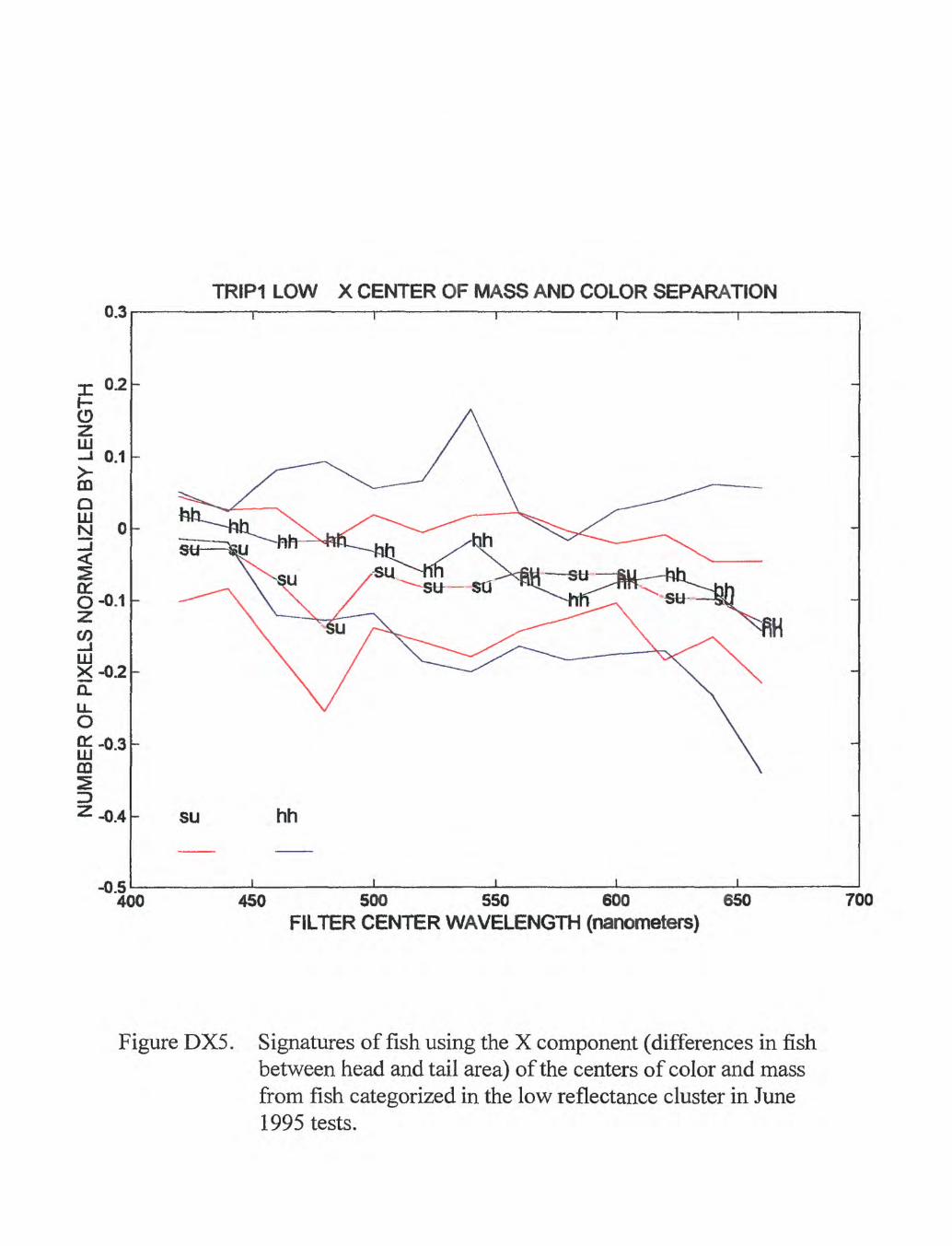
TRIP1 LOW X CENTER OF MASS AND COLOR SEPARATION0.3

0.2

0.1

CD

LJJ

feQ LU N

0-0.1

LU X-0.2CL LL O

CD2ID

-0.5 400

SU hh

450 500 550 600FILTER CENTER WAVELENGTH (nanometers)

650 700

Figure DX5. Signatures offish using the X component (differences in fish between head and tail area) of the centers of color and mass from fish categorized in the low reflectance cluster in June 1995 tests.

TRIP2 LOW X CENTER OF MASS AND COLOR SEPARATION0.3

0.2

ILU

0.1

O LU N

0-0.1-2L

CO

LU X-0.2CL

8r°-3m

-0.4

-0.5 400

su chj

450 500 550 600FILTER CENTER WAVELENGTH (nanometers)

650 700

Figure DX6. Signatures of fish using the X component (differences in fish between head and tail area) of the centers of color and mass from fish categorized in the low reflectance cluster in September 1995 tests.

, tf* TRIP1 HIGH Y NORMALIZED COLOR MOMENTS OF INERTIA

<3-5

EELU Z 3

u_ OCO O ch- 2-5LU

1 2OL Od 1 -5oQLU ^N 1

01 0.5 Oz

-0.5 400

sb - sb sb - sb--st

~shl

shs shl cs sb

450 500 550 600 650 FILTER CENTER WAVELENGTH (nanometers)

700

Figure MYl. Signatures of fish using the Y component (differences ofreflectivity vary between the center of the fish and either the dorsal and/or ventral areas) in the normalized moment of color for fish categorized in the high reflectance cluster in June 1995 tests.

Y N

OR

MA

LIZ

ED

CO

LOR

MO

ME

NT

S O

F IN

ER

TIA

co £

o.

3

GOCD

o

o

jj^ !

"S

- o*

55

2 "*

£-IS

1"

rl-

<T)

O)

OQ52

. O

E?

2.

n> co

<

O th

B 5T

co?S

B-

rg §

OQr\

i "->

*

.

fD 3

O

O ^

I 8

o

o^

pj

>J^ ^

^ *

*

J J

O o g s

co o

6

FS 3J O m » I

7] lg

p UI

(0 (0

UI

i. I Q o 73 I O

O o 7] m 1 o n

m

10

< 8

x10,-s TRIP1 MEDIUM Y NORMALIZED COLOR MOMENTS OF INERTIA

6

o: LU

oCO

1O

O OQ 0 111 N

tr o

-2

cf we sq rb

400 450 500 550 600FILTER CENTER WAVELENGTH (nanometers)

650 700

Figure MY3. Signatures of fish using the Y component (differences ofreflectivity vary between the center of the fish and either the dorsal and/or ventral areas) in the normalized moment of color for fish categorized in the medium reflectance cluster in June 1995 tests.

14

12 <

QL LU 10

x 10-s TRIP2 MEDIUM Y NORMALIZED COLOR MOMENTS OF INERTIA

CO

LU

8

6O

Q£ 4

g oO 2QLUNIJ 0<

O -2

-6 400

Cf we sq sr

450 500 550 600 650FILTER CENTER WAVELENGTH (nanometers)

700

Figure MY4. Signatures offish using the Y component (differences ofreflectivity vary between the center of the fish and either the dorsal and/or ventral areas) in the normalized moment of color for fish categorized in the medium reflectance cluster in September 1995 tests.

14

12

LU10

u_O 8 CO

zLU e

o: 4 o_JoO 2Q UJ N Zi 0

onO -2

x10 TRIP1 LOW Y NORMALIZED COLOR MOMENTS OF INERTIA

SU hh

400 450 500 550 600FILTER CENTER WAVELENGTH (nanometers)

650 700

Figure MY5. Signatures of fish using the Y component (differences ofreflectivity vary between the center of the fish and either the dorsal and/or ventral areas) in the normalized moment of color for fish categorized in the low reflectance cluster in June 1995 tests.

10

< 8

01z

oCO

Z LU

o: 2 oo oQ 0UJN

-2

x 10-s TRIP2 LOW Y NORMALIZED COLOR MOMENTS OF INERTIA

gj:>j-=ehp:=66jg

su hh chj

400 450 500 550 600 650FILTER CENTER WAVELENGTH (nanometers)

700

Figure MY6. Signatures of fish using the Y component (differences ofreflectivity vary between the center of the fish and either the dorsal and/or ventral areas) in the normalized moment of color for fish categorized in the low reflectance cluster in September 1995 tests.

3.5

< 3

LU Z ~ 2.5O CO

1 2

O2(£ 1.5O

O OQ 1LUN

x 10-* TRIP1 HIGH X NORMALIZED COLOR MOMENTS OF INERTIA

a: o

0.5

-0.5 400

*hr~ shL-*hH- shl

shs shl cs sb

450 500 550 600 650FILTER CENTER WAVELENGTH (nanometers)

700

Figure MXI. Signatures of fish using the X component (differences ofreflectivity vary between the center of the fish and either the head and/or tail areas) in the normalized moment of color for fish categorized in the high reflectance cluster in June 1995 tests.

X N

OR

MA

LIZ

ED

CO

LOR

MO

ME

NT

S O

F IN

ER

TIA

CD

I

K1 5

5

co

o Q3 -

(D j M

^

<-*

CDO

O

*^

W

S' s

? p

S,CD

S

. H

i_

i.C

L C

* g

»B

'cr CD

\~

~/

^

j~7

'

B-

g

OQ

^r1

cii ?

Xsis

3 B-

§

§ 2

31

o o

o is

(o

n

B* g

»

s-a

o th

^2-1

?i

S? o Io o

; n>

r1 co

s) 73

Og

m o

73 I m 1

o

in

(0

v>

CT

(A

CT W

CT

N)

tn

X o 73 B O

O o o

m 3 m 7J j!

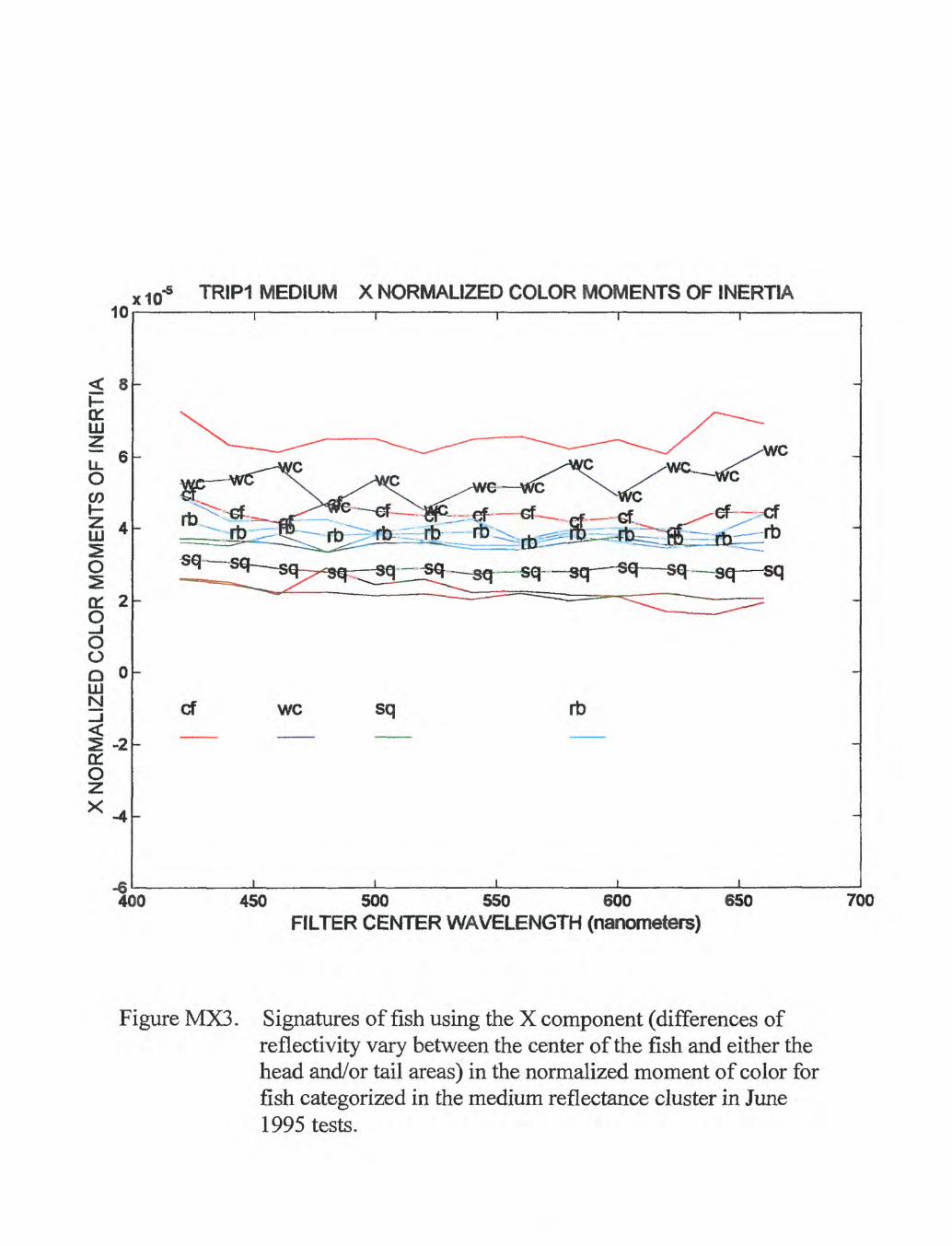
10

< 8

x 10-s TRIP1 MEDIUM X NORMALIZED COLOR MOMENTS OF INERTIA

or in6U-

OCO

i 4oo: 2 go oQ o mN

a: o

-2

-6 400

we

sq sq- scf - sq- sq $3 s% sq

cf we sq rb

450 500 550 600 650 FILTER CENTER WAVELENGTH (nanometers)

700

Figure MX3. Signatures offish using the X component (differences ofreflectivity vary between the center of the fish and either the head and/or tail areas) in the normalized moment of color for fish categorized in the medium reflectance cluster in June 1995 tests.

14

12

P

LU 10

U)

ZLU fi 2 6

O 2 tt 4

g oO 2 Q LU N Ii 0

01 O -22X

, 10-5 TRIP2 MEDIUM X NORMALIZED COLOR MOMENTS OF INERTIA

-6 1 400

cf we sq sr

450 500 550 600 650 FILTER CENTER WAVELENGTH (nanometers)

700

Figure MX4. Signatures of fish using the X component (differences ofreflectivity vary between the center of the fish and either the head and/or tail areas) in the normalized moment of color for fish categorized in the medium reflectance cluster in September 1995 tests.

10

< 8

a: in2

oCO

1 4s o so: 2 go o Q oinN

x 10-s TRIP1 LOW X NORMALIZED COLOR MOMENTS OF INERTIA

a: o

-2

su hh

400 450 500 550 600FILTER CENTER WAVELENGTH (nanometers)

650 700

Figure MX5. Signatures of fish using the X component (differences ofreflectivity vary between the center of the fish and either the head and/or tail areas) in the normalized moment of color for fish categorized in the low reflectance cluster in June 1995 tests.

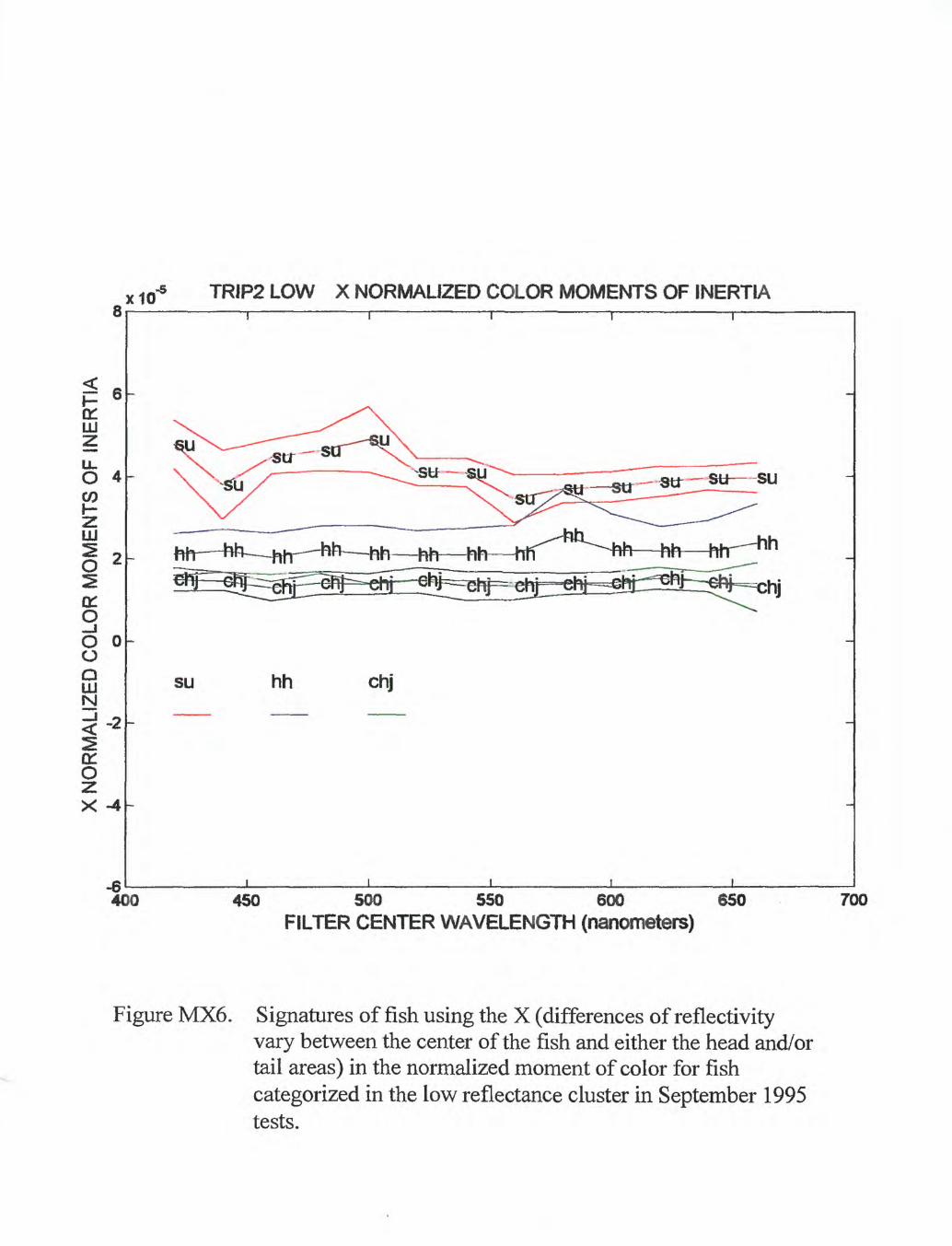
x10" TRIP2 LOW X NORMALIZED COLOR MOMENTS OF INERTIA

DC LU

O 4

LU

o: go o oo LU N_i )Ia: oX -4

-6 400

hh hh hrf^

su hh chj

450 500 550 600 650FILTER CENTER WAVELENGTH (nanometers)

700

Figure MX6. Signatures of fish using the X (differences of reflectivityvary between the center of the fish and either the head and/or tail areas) in the normalized moment of color for fish categorized in the low reflectance cluster in September 1995 tests.

10

< 8

DC LU

il 6 oCO

x ltf« TRIP1 LOW X NORMALIZED COLOR MOMENTS OF INERTIA

01 2 OO O Q 0

aDC O

-2

-6 400

su hh

450 500 550 600FILTER CENTER WAVELENGTH (nanometers)

650 700

Figure MX5. Signatures of fish using the X component (differences ofreflectivity vary between the center of the fish and either the head and/or tail areas) in the normalized moment of color for fish categorized in the low reflectance cluster in June 1995 tests.

TRIP2 LOW X NORMALIZED COLOR MOMENTS OF INERTIA

a: LU

O 4

LU

o:o _iO 0oQ LU N

OHo z.X -4

nfr hh htr "** hh

su hh chj

400 450 500 550 600 650FILTER CENTER WAVELENGTH (nanometers)

700

Figure MX6. Signatures of fish using the X (differences of reflectivityvary between the center of the fish and either the head and/or tail areas) in the normalized moment of color for fish categorized in the low reflectance cluster in September 1995 tests.