Experimenting with Entrepreneurship:

The Effect of Job-Protected Leave

⇤

Joshua D. Gottlieb

University of British Columbiaand NBER

Richard R. Townsend

University of California San DiegoTing Xu

University of British Columbia

July 17, 2016

Abstract

Do potential entrepreneurs remain in wage employment because of the danger thatthey will face worse job opportunities should their entrepreneurial ventures fail? Usinga Canadian reform that extended job-protected leave to one year for women giving birthafter a cutoff date, we study whether the option to return to a previous job increasesentrepreneurship. A regression discontinuity design reveals that longer job-protectedleave increases entrepreneurship by 1.8 percentage points. The results are driven bymore educated entrepreneurs, starting firms that survive at least five years and hirepaid employees, in industries where experimentation is more valuable.

JEL Classification: L26, J13, J16, J65, J88, H50Keywords: Entrepreneurship, Risk-Aversion, Job-Protected Leave, Career, Real Option, Experimentation

⇤Gottlieb: Joshua.Gottlieb@ubc.ca. Townsend: rrtownsend@ucsd.edu. Xu: ting.xu@sauder.ubc.ca. We are grate-ful to Shai Bernstein, Ing-Haw Cheng, Gordon Dahl, Thomas Hellmann, Kai Li, Gustavo Manso, Kevin Milligan,Ramana Nanda, Carolin Pflueger, Matt Rhodes-Kropf, Elena Simintzi, conference and seminar participants at Cal-tech/USC, NBER, Stanford, and UBC, and especially our discussants Paige Ouimet and Joshua Rauh for valuablecomments. Gottlieb thanks the Stanford Institute for Economic Policy Research and Federal Reserve Bank of SanFrancisco for their hospitality while working on this project, and the Social Sciences and Humanities Research Coun-cil of Canada for support. We are indebted to Statistics Canada, SSHRC, and the staff at the British ColumbiaInteruniversity Research Data Centre at UBC for facilitating data access. The research and analysis are based ondata from Statistics Canada and the opinions expressed do not represent the views of Statistics Canada.

1 Introduction

Entrepreneurship has long been thought to play a critical role in innovation, job creation and

economic growth (Schumpeter, 1911). There is now a large body of empirical evidence in support of

this view (e.g. King and Levine, 1993; Levine, 1997; Beck, Levine and Loayza, 2000; Levine, Loayza

and Beck, 2000; Guiso, Sapienza and Zingales, 2004). Yet only a small fraction of the population

undertakes entrepreneurial endeavors. For example, in the United States, only 6.6 percent of the

labor force is self-employed (World Bank, 2015).

While regulation and capital access are previously-documented impediments to starting a busi-

ness,1 perhaps the most fundamental reason people might avoid entrepreneurship is its risk. Starting

a new business is inherently risky since a wide range of outcomes is possible and the ex ante likelihood

of substantial success is low. Perhaps most importantly, downside outcomes for entrepreneurs are

exacerbated by career considerations. If a potential entrepreneur leaves her secure corporate job to

start a company that ultimately fails, she may subsequently have trouble finding non-entrepreneurial

employment nearly as good as she could have obtained without the failure.2

This idea of career considerations motivates the widely-held belief that entrepreneurship in-

creases during recessions. Workers who have already lost their job face a lower opportunity cost

of trying to start a new business, though opinions vary as to whether entrepreneurship increased

during the Great Recession (Fairlie, 2010; Shane, 2011). In this paper, we use a natural experiment

to investigate the relationship between entrepreneurship and career considerations. In particular,

we examine whether granting employees extended leaves of absence, with guaranteed options to

return to their jobs, increases entry into entrepreneurship.

While employees do not often have the option to take leaves for the purpose of starting a business,1See, for example, Evans and Jovanovic (1989); Holtz-Eakin, Joulfaian and Rosen (1994a,b); Hurst and Lusardi

(2004); Bertrand, Schoar and Thesmar (2007); Mel, McKenzie and Woodruff (2008); Kerr and Nanda (2009); Adelino,Schoar and Severino (2015); Schmalz, Sraer and Thesmar (2015); Mullainathan and Schnabl (2010); Bruhn (2011);Branstetter, Lima, Taylor and Venâncio (2014)

2According to entrepreneurs themselves, their two main fears are financial risk and the fear of losing a stableprofessional job (Brinckmann, 2016). The latter concern is supported by the evidence. Ferber and Waldfogel (1998),Williams (2002), Bruce and Schuetze (2004), Niefert (2006), and Kaiser and Malchow-Moller (2011) all documentthat previously self-employed individuals earn lower wages upon returning to wage employment than continuouslywage-employed individuals.

1

governments often require that leaves be permitted surrounding the birth of a child. Such leaves,

if sufficiently long, could in principle be used to explore a business idea while retaining the option

to return to one’s previous job. We exploit a reform to Canadian maternity leave laws that took

place in 2000. The reform extended job-protected leave entitlements to one year, approximately a

five month increase. In contrast, the US mandates only three months of leave in total. Given that

US law expects employees to return to work after three months, workers in Canada may be able to

use their substantial additional time to test the viability of a business idea, even with a new child

in the household.

Indeed, anecdotal evidence suggests that entry into entrepreneurship among Canadian women

increased following the reform. According to the Vancouver Sun, “a growing number [of mothers] are

using their maternity leave—now a full year in Canada—to either plan or start a new professional

direction in life. . . longer maternity leaves are making it easier for women to try their hand at

starting a business” (Morton, 2006). Danielle Botterell, author of the Candian book Moms Inc.,

said in an interview with the Globe and Mail, “We think the trend of mompreneurship, particularly

in this country, really took off when the government extended maternity leave to a year” (Pearce,

2011). According the Financial Post, a Canadian business newspaper, “there is a new breed of

female entrepreneurs using their maternity leaves to incubate real businesses” (Mazurkewich, 2010).

One entrepreneur interviewed used her maternity to start amassing clients, explaining that “my

maternity leave was my security blanket.” In her interpretation, job-protected leave time allowed

for low-risk experimentation with entrepreneurship (Karol, 2012).

Our empirical strategy exploits the fact that implementation of maternity leave reform in Canada

was tied to the date a woman gave birth. In particular, mothers who gave birth on or after December

31, 2000 were eligible for the extended job-protected leave. Those who gave birth even one day

before were not. Given that there are limitations on the extent to which the timing of births can

be controlled, “gaming” around the cutoff date is likely to be limited. Consistent with the difficulty

of gaming, we find no evidence of a jump in the birth rate after the cutoff date. Moreover, the

2

observable characteristics of those who gave birth just before and after the cutoff suggest that they

are similar in terms of age, education, and ethnicity. Thus, the way that the reform was implemented

lends itself to examination with a regression discontinuity design.

In particular, we examine whether mothers who gave birth just after the cutoff date are discon-

tinuously more likely to be entrepreneurs as of the next census five years later. We are unable to

look at shorter-term effects because the 2001 Census is too close to the reform cutoff date. Nonethe-

less, the benefit of looking at long-term outcomes is that the results cannot merely reflect transitory

entry into entrepreneurship. We find that the increase in job-protected leave entitlements leads to

approximately a 1.8 percentage point increase in entrepreneurship among mothers. Compared to

an approximately 5 percent base rate, this represents an economically significant increase of around

35 percent. This baseline result is robust when examining different windows around the cutoff date,

different methods of fitting the pre- and post- trends, and different definitions of entrepreneurship.

The effect is stronger for women with more human and financial capital. Moreover, the effect is

concentrated in industries where experimentation arguably plays a more important role: those with

high startup capital requirements, high failure rates, and high cashflow volatility.

These findings have more economic significance if the entry into entrepreneurship we observe

involves high-quality entrepreneurs as opposed to low-quality entrepreneurs. Several pieces of evi-

dence speak to the quality of the new entrepreneurs. First, we measure businesses that still exist

five years after the reform. If the reform only increased low-quality entrepreneurship, we would not

expect to see long-run effects because the marginal businesses would fail within that time frame.

Further, we find that the effect of the reform on entrepreneurship is significantly stronger for mothers

with ex ante characteristics that predict higher quality businesses. In particular, those with more

education, work experience, and access to capital respond more strongly to the reform. We further

distinguish high-quality entrepreneurship from low-quality entrepreneurship by examining whether

a business has paid employees. We find that the reform leads to an increase in entrepreneurs that

hire employees but has no effect on non-job-creating entrepreneurship. These results also help to

3

rule out the possibility that longer leaves simply lead to skill degradation or changes in preferences

away from wage employment.

While our results directly involve entry into entrepreneurship by recent mothers, it is quite

plausible that they generalize beyond that population. For example, if engineers at large technology

companies were given the ability to take job-protected leave unrelated to the birth of a child, our

results suggest that such an intervention might lead to the creation of more technology startups.

To be sure, policy interventions of this sort have other costs and benefits that we do not measure

here. So we do not aim to make welfare statements about such policies. Our objective is to shed

light on whether career considerations indeed represent a major impediment to entrepreneurship,

using these policies as an empirical tool.

Our paper contributes to a growing literature that views entrepreneurship as a series of exper-

iments (see Kerr, Nanda and Rhodes-Kropf, 2014, for an overview). While many entrepreneurial

projects may be negative NPV in a static sense, entrepreneurs can engage in cheap experiments

that reveal information about the project’s prospects. Conditional upon that information being

favorable, the project may become positive NPV; thus, there is value in the real option to con-

tinue. In closely related work, Manso (2014) and Dillon and Stanton (2016) model the dynamics

of experimentation in self-employment and quantify this option value. According to this exper-

imentation view, frictions to experimenting are the chief impediment to entrepreneurship. Such

frictions can be due to regulation (Klapper, Laeven and Rajan, 2006), technology (Ewens, Nanda

and Rhodes-Kropf, 2015), organizational constraints (Gompers, 1996), or financing risk (Nanda and

Rhodes-Kropf, 2013, 2014). In our setting, job-protected leaves could reduce the cost of experimen-

tation by giving entrepreneurs the ability to test an idea’s viability without the risk of long-term

negative career consequences.

More broadly, we contribute to a large literature on factors that discourage entrepreneurship.

Entry regulations limit entrepreneurship both across (Djankov, Porta, Lopez-de Silanes and Shleifer,

2002; Desai, Gompers and Lerner, 2003; Klapper, Laeven and Rajan, 2006) and within countries

4

(Mullainathan and Schnabl, 2010; Bruhn, 2011; Branstetter, Lima, Taylor and Venâncio, 2014).

Much work has examined whether relaxing financial constraints increases entrepreneurship (Evans

and Jovanovic, 1989; Holtz-Eakin, Joulfaian and Rosen, 1994a,b; Hurst and Lusardi, 2004; Bertrand,

Schoar and Thesmar, 2007; Mel, McKenzie and Woodruff, 2008; Kerr and Nanda, 2009; Adelino,

Schoar and Severino, 2015; Schmalz, Sraer and Thesmar, 2015), and whether entrepreneurship

training programs or exposure to entrepreneurial peers generate spillovers (Karlan and Valdivia,

2011; Lerner and Malmendier, 2013; Drexler, Fischer and Schoar, 2014; Fairlie, Karlan and Zinman,

2015). This paper differs in its focus on career considerations. We are not aware of any other work

examining whether potential entrepreneurs hesitate to take the plunge because they are afraid to

worsen their fallback option. Our findings are consistent with Manso (2011), who shows that the

optimal contract to motivate innovation (or experimentation more generally) involves a commitment

by the principal not to fire the agent.

In recent work, Hombert, Schoar, Sraer and Thesmar (2014) examine a French reform to unem-

ployment insurance (UI). Prior to the reform, unemployed workers would stop receiving UI payments

if they started a business. Following the reform, starting a business no longer required giving up

these benefits. Hombert et al. (2014) study how this reform affects the composition of new en-

trepreneurs. New firms started in response to the reform are, on average, smaller than start-ups

before the reform, but they are just as likely to survive and to hire employees. We differ in our

focus on the career considerations of potential entrepreneurs, rather than the quality of the marginal

entrepreneur.

Finally, our paper also contributes to a large literature on the effects of maternity leave on

labor market outcomes (Ruhm, 1998; Klerman and Leibowitz, 1999; Waldfogel, 1999; Baker and

Milligan, 2008a; Lalive and Zweimüller, 2009; Lalive, Schlosser, Steinhauer and Zweimüller, 2013;

Schönberg and Ludsteck, 2014). Overall, the literature finds that more generous leave entitlements

do delay mothers’ return to work. However, evidence on the relationship between leave duration and

subsequent outcomes is mixed. A key empirical challenge has been to find exogenous variation in

5

leave-taking by mothers. Our paper adds to this literature by examining entry into entrepreneurship,

rather than wages and job continuity. Moreover, the way the reform in Canada was implemented

allows us to use a regression discontinuity design to identify causal effects. Thus far, such an

empirical strategy has only been possible with data from Norway, where leaves increased more

gradually over time—from 18 weeks to 35 weeks in 6 separate reforms from 1977 to 1992 (Dahl,

Løken, Mogstad and Salvanes, 2013; Dahl, Løken and Mogstad, 2014).

This paper proceeds as follows. Section 2 presents a simple conceptual framework showing how

job-protected leave could encourage entry into entrepreneurship. Section 3 discusses the data used

in the study. Section 4 discusses the details of maternity leave in Canada. Section 5 discusses our

empirical strategy. Section 6 presents the results. Section 7 concludes.

2 Conceptual Framework

In order to fix ideas, we present a stylized model of the self-employment decision in our context. The

model describes how the choice to explore self-employment can respond to parental leave policy, and

generates predictions that we will test empirically. Consider a potential worker whose background

option is a job that pays a constant real income of y.3 At time 0, she has a child and takes an initial

maternity leave. During this time period, job-protected leave is guaranteed in all different policy

regimes. So, regardless of any policy changes we will consider, she always has the right to resume

the wage-y job at time 1.

At time 1, she has three choices. She can stay at home with the child and receive a non-pecuniary

benefit b but earn no income. She can resume employed work at income y, but in that case she has

to pay child care costs of k � 0. Or she can take the risk of starting a business.

When starting a business, the entrepreneur chooses an effort level e, which influences the po-

tential payoff. This effort has a convex cost, scaled by an effort cost parameter ↵ > 0; the total

cost is ↵e2. We assume that ↵ is distributed uniformly in the population on [0, 1], and each agent

3We abstract away from discounting, inflation, and wage growth. So all incomes and costs can be thought of asreal time-0 values.

6

knows her own ↵ when making her choices. An entrepreneur also has to pay for child care, so the

total cost of entrepreneurship in the first period is ↵e2 + k. We assume that the effort cost is only

incurred once.

There are two possible payoffs if she starts the business. With probability ⇡ 2 (0, 1), the business

succeeds and generates a payoff of �e where � > 0 is another parameter. We think of this payoff

as all-inclusive—for example, it could include non-monetary benefits of self-employment. With

probability 1� ⇡, the business fails and the gross payoff is 0.

We simplify matters at time 2 by assuming that she always returns to some form of work,

whether wage employment or self-employment. If she previously returned to wage employment at

time 1, her wage is unchanged at y. If she became an entrepreneur at time 1, and the business was

successful, we assume that it continues to thrive at time 2 and the payoff is again �e. Someone

who found it worthwhile to take the risk of entrepreneurship will not return to wage employment

if self-employment is successful, since the return is unchanged and there is no additional risk or

effort cost. On the other hand, if she stayed on leave or if the time-1 business failed, the empirical

evidence predicts that she would suffer a salary reduction should she return to wage employment at

time 2 (Bertrand, Goldin and Katz, 2010; Bruce and Schuetze, 2004). We express this wage cut as a

proportional reduction from y to (1� �)y where � < 1 is a parameter. When a policy guaranteeing

job-protected leave is introduced, we interpret it as reducing or eliminating the penalty � from

taking time off. Table 1 summarizes the payoffs in each time period under each choice, and Figure

1 illustrates the timing.

The people we consider are those with parameters such that y(1 + �) > b + k. This condition

implies that the mothers we study prefer to return to work at time 1 over spending their extended

leave purely on child care. Of course this condition will not hold for all mothers, but those who

prefer taking the maximum time off are unlikely to respond to our policy change by becoming

entrepreneurs.4 The condition shows that higher wages and a higher penalty for absence from the

labor market (�) make working preferable to extended leave. Higher childcare costs and higher4In fact, we can show that their entrepreneurship response is opposite that of those who satisfy y(1 + �) > b+ k.

7

benefits make it better to stay at home. This decision depends only on fixed parameters, and not

the heterogeneous effort cost ↵.

Given this framework, we can predict who will try her hand at entrepreneurship. We simply com-

pare the expected payoffs to entrepreneurship and wage employment at time 1. These comparisons

yield a threshold rule in the effort cost ↵. Those with effort costs satisfying

↵ <�2⇡2

2y � y(1� ⇡)(1� �)⌘ A (1)

will become entrepreneurs. The right-hand side of inequality (1) defines the threshold A for the

effort cost ↵. Those with effort costs ↵ > A will return to paid employment at time 1, while those

with lower values of ↵ will start a business.

Since ↵ ⇠ Unif[0, 1], the threshold A for the entrepreneurship decision is also equal to the share

of potential entrepreneurs who will choose entrepreneurship. We can now consider the effect of a

policy guaranteeing mothers the option to return to their previous job at time 2. This policy reduces

or eliminates the wage penalty � from taking time off. To compute its effect on the share choosing

self-employment at time 1, we differentiate the self-employment share A with respect to �:

dA

d�= � �2⇡2(1� ⇡)

y [2� (1� ⇡)(1� �)]2(2)

Both the numerator and denominator in this fraction are positive, so equation (2) is negative overall.

Reducing the wage penalty increases the share choosing self-employment. The effect is increasing

in the return to self-employment �, and decreasing in the market wage y. The �2⇡2 term in the

numerator of equation (2) comes from the entrepreneur’s optimal effort decision. Conditional on

becoming an entrepreneur, more skilled workers have higher returns to effort, so choose a higher

effort level (the optimal effort choice is e⇤ =�⇡

↵). The optimal effort choice responds to and

reinforces � and ⇡, leading to the quadratic term.

To determine whether these effects are larger for high- or low-human capital workers, we have to

8

interpret human capital in light of the model. If human capital only shows up in wages y, then the

effects are unambiguously decreasing in human capital⇣

d2Ad�dy > 0

⌘. If human capital only shows up

in the returns to entrepreneurship �, then the effects are increasing in human capital⇣

d2Ad�d� < 0

⌘.

Perhaps the most natural interpretation of human capital is that both entrepreneurship returns and

market wages (� and y) increase proportionally to each other and to an underlying skill level. If

this is so, then the return to self-employment dominates and higher-human-capital workers will be

more responsive to changes in the wage penalty �.5

Finally, we consider variation in the effect of � depending on the level of risk involved in en-

trepreneurship. Observe in equation (2) that the wage penalty has no effect on entrepreneurship

when ⇡ = 0 or ⇡ = 1—when there is no uncertainty in the payoff of entrepreneurship. Only

for intermediate values of ⇡—when entrepreneurship involves elevated risk—does the wage penalty

matter. So the model predicts bigger effects of the wage penalty on entrepreneurship as the risk of

entrepreneurship increases from either extreme.

3 Data

The data used in this paper come primarily from the Canadian Census of the Population, which is

administered every five years by Statistics Canada. The census enumerates the entire population of

Canada. Eighty percent of households receive a short census questionnaire, which asks about basic

topics such as age, sex, marital status, and mother tongue. Twenty percent of households receive

the long-form questionnaire, which adds many additional questions on topics such as education,

ethnicity, mobility, income, employment, and dwelling characteristics. Respondents to the long

form survey typically give Statistics Canada permission to directly access tax records to answer the

income questions. Participation in the census is mandatory for all Canadian residents. Aggregated

data from the census are available to the public. Individual-level data are only made publicly

available 92 years after each census and in some cases only with the permission of the respondent.5Specifically, let � = w1h and y = w2h, where w1, w2 > 0 are constants and h measures human capital. Then

equation (2) becomes dAd� = � hw2

1⇡2(1�⇡)

w2[2�(1�⇡)(1��)] . Then d2Ad�dh < 0 so the effect of � is increasing in human capital.

9

However, for approved projects, Statistics Canada makes the micro-data from the long form survey

available for academic use. We use these confidential micro-data in our study. While the data are at

the individual level, they are still anonymized. Moreover, the individual and household identification

codes are not consistent across census years. So although the census is administered to the whole

population every five years, it is not possible to form a panel and our data are purely cross-sectional.

Our primary sample consists of mothers from the 2006 census who (we infer) had a child within

5 months of the December 31, 2000 reform date. There are 118,470 such mothers in the census.

Due to restrictions from Statistics Canada, all of our results (including observation counts) are

reported using census weights. Because participation in the census is mandatory and the 20 percent

of households selected for the long form survey are random, the weights are generally very close to 5

for all respondents. That is, one observation in the sample data is representative of approximately

5 observations in the population data. Because the weights are so uniform, our results change little

when they are unweighted.

One key variable for this study is the date on which a woman gave birth. While the census does

not directly record this information, it can be inferred fairly well from the birth dates of children

residing in the same household. In particular, the census records family relationships within a

household and the date of birth for all members of the household. Therefore, we assume that a

mother gave birth on the birth dates of the children residing in the same household. Of course, there

is some measurement error in our inferred dates of child birth. For example, we would incorrectly

infer dates of child birth for women residing in a household with adopted children or step-children.

Similarly, for women who do not reside in the same household as their children, we would incorrectly

infer that they never gave birth.6 We think that this measurement error is likely small in magnitude

and, if anything, it would bias us against finding the effects we estimate.

The other key variable for our study is entrepreneurship, which we proxy for with self-employment,

as is common in the literature. Respondents to the long form census must provide information on

6We use children reported in the 2006 census to infer child birth dates in a window around December 31, 2000;therefore the relevant children would be around five years old as of the 2006 census date.

10

both their total income and self-employment income. In most cases, this information is obtained

directly from their tax filings. Our primary definition of self-employment is someone who receives

at least 50 percent of her total income from self-employment.7 Separately, respondents must also

report whether they consider themselves self-employed based on their primary job. If they report

being self-employed, they also indicate whether their business has paid employees. We favor the

income-based measure as it comes from administrative data. However, we show in robustness tests

that our results are similar when using self-reported self-employment. Note that both measures of

self-employment include individuals who have incorporated their businesses or hired paid employees.

Table 2 shows basic summary statistics for mothers and for fathers who had a child within 5

months of the December 31, 2000 reform date. While the sample is selected based on the inferred

birth of a child around December 31, 2000, the summary statistics reflect information as of the 2006

census. In our sample, 4.41 percent of mothers are self employed as of 2006 when using the definition

based on self-employment income. In addition, 2.68 percent both identify themselves as being self-

employed and have over 50 percent of their income over the past year from self-employment. The

average mother in the sample is approximately 32.8 years old and has 1.76 children as of 2006.

About 28.6 percent are college graduates. The rate of self-employment for fathers is higher, as are

age and education. Note that there are fewer fathers than mothers in the sample because there are

more households with only a mother present than households with only a father present.

4 Maternity Leave Policy In Canada

Canada’s ten provinces8 have significant legal and fiscal autonomy, and in particular have pri-

mary responsibility for labor legislation. Despite this autonomy, legislatively guaranteed maternity

leave—the right to return to a pre-birth job after a specified period of absence—has several com-

mon features across the provinces. First, employees are protected from dismissal due to pregnancy.

7Canadian taxes are assessed based on individual income, not combined spousal income as in the US Thus ourdata record self-employment and wage employment income for each individual.

8In addition to the ten provinces, whose combined population is 34 million, Canada has three territories with acombined population of 100,000, located north of 60 degrees latitude.

11

Second, a maximum period for the leave is always prescribed, and the provinces do not mandate

any paid leave. Initially the laws of several provinces provided guidance on how the period of leave

should be split pre- and post-birth, but current practice is to leave this to the discretion of the

mother and employer. Third, the laws specify a minimum period of employment for eligibility. This

varies widely: initially 52 weeks of employment was common, although the recent trend is toward

shorter qualification periods. Fourth, most laws specify which terms of employment are preserved

during the leave and any responsibility of the employer to maintain benefits. Finally, the laws of

some provinces establish rules for extending leaves because of medical complications or pregnancies

that continue after term (Baker and Milligan, 2008b).

While provinces only mandate a period of unpaid leave, partial income replacement is provided

by the federal employment insurance system. Prior to 2001, employment insurance provided partial

income replacement for 25 weeks surrounding the birth of a child (a 2-week unpaid waiting period

followed by a 25-week paid leave period). In 2001, the Employment Insurance Act was reformed to

allow for up to 50 weeks of partial income replacement (a 2-week unpaid waiting period followed

by a 50-week paid leave period). Those on leave receive 55 percent of their normal income up to a

maximum determined each year based on mean income levels (at the time $413 CAD per week, or

about $275 USD). Of course temporary income replacement is less useful if one’s pre-birth employer

does not approve of the leave, and the absence were to cost the new mother her job. Prior to the 2001

reform to the Employment Insurance Act, provinces required that employers grant anywhere from 18

to 35 weeks of job-protected leave surrounding the birth of a child (with the exception of Quebec,

which already required 70 weeks). Following the reform, all provinces increased the mandated

guarantee to at least 52 weeks to match the new income replacement period set by employment

insurance (including the 2-week waiting period). Table 3 shows the maximum leave period by

province, before and after the 2001 reform. The average province went from approximately 35

weeks to 54 weeks, an increase of almost 5 months. Given that maternity leave entitlements usually

increase gradually over time, this reform represents one of the largest year-over-year increases in

12

any country.

5 Empirical Strategy

An important aspect of the reform’s implementation for our purposes is that it was tied to the

date a woman gave birth. Those who gave birth on or after December 31, 2000 were entitled to

an extended leave. Those who gave birth even a day before were not. Despite unhappiness among

those who just missed the cutoff, no exceptions were made to this policy, even in cases of premature

births (Muhlig, 2001).

Figure 2 illustrates our setup graphically using the sample of mothers who filled out the long form

census questionnaire in 2006. In both panels, the horizontal axis represents the date of childbirth

relative to the reform date. The vertical axis shows the maximum weeks of paid and unpaid leave,

in Panels A and B respectively, available to the mother based on the date and province where she

lived at the time of the birth. We proxy for this location with the respondent’s answer to the

2006 census question about her province of residence five years earlier. The dots represent means

for births in that week and the lines fit a cubic trend on each side of the cutoff with 95 percent

confidence intervals. In Panel A there is no variation within a birth date as paid leave is determined

at the federal level. Thus, all mothers in our sample who gave birth before December 31, 2000, were

eligible for exactly 25 weeks of paid leave; those who gave birth after were eligible for 50 weeks. In

Panel B, there is some variation induced by the fact that different provinces have different unpaid

leave policies. On average, women in our sample who gave birth before the reform date were eligible

for approximately 40 weeks of total job-protected leave; those who gave birth after were eligible for

57 weeks.

While Figure 2 illustrates that there was a discontinuous jump in both paid and unpaid leave

eligibility for mothers who gave birth around the reform, it does not show whether there was a

discontinuous jump in the amount of leave actually taken. If the reform had no effect on actual

leave-taking, we would not expect to find an effect on entrepreneurship. Unfortunately, census

13

respondents do not report the amount of leave they took with each child, preventing us from creating

a figure analogous to Figure 2 showing the actual weeks of leave taken. However, the census data

do allow for a cruder analysis along these lines. While respondents do not retrospectively report

the length of previous leaves taken, they do report whether they are currently on leave as of the

census date. We therefore trace out the probability of a respondent being on leave on the census

date as a function of the number of weeks between her most recent child’s birth and the census

date. We do this separately using data from the 1996 and 2006 censuses. Figure 3 shows that,

in all weeks following birth, the probability of employed mothers being on leave is indeed greater

in the post-reform period. Of course, given that we are comparing leave taking behavior in two

periods that are ten years apart, it is possible that such behavior changed for reasons other than

than the reform. However, Baker and Milligan (2008a) study the same Canadian reform using a

difference-in-differences estimation framework—they use panel data, but have a sample too small

for our RDD estimation strategy. Their results comport with Figure 3: the reform increased the

length of leave actually taken by mothers. We repeat the same exercise for fathers and, consistent

with Baker and Milligan (2008a), find little change in leave-taking behavior from 1996 to 2006. It

thus appears that there was a discontinuous increase in the amount of leave available to and taken

by mothers who gave birth just after the December 31, 2000 cutoff date.

Aside from leave-taking, women on each side of the cutoff are likely to be similar in terms of

other characteristics. The reform thus lends itself naturally to analysis with a sharp regression

discontinuity design (RDD). Our hypothesis is that the additional leave time may promote entry

intro entrepreneurship by giving individuals the opportunity to test the viability of business ideas

without risking harm to their current career paths. To test this hypothesis we estimate standard

parametric RDD models of the form:

yit = � · Postt +KX

k=1

�k · EventT imekt +KX

k=1

�k · EventT imekt ⇥ Postt + ✏it (3)

where yit is an outcome of interest for individual i who gave birth at time t, EventT imet is the

14

date of a child’s birth relative to the reform date, Postt is an indicator variable equal to one if the

birth is on or after the reform date, and K is the degree of the polynomial time trend that we fit

separately on either side of the cutoff. In robustness tests we estimate this equation with different

polynomial degrees and non-parametric control functions.

Our primary outcome of interest is an indicator equal to one if individual i is an entrepreneur

as of the 2006 census date, as defined in Section 3. Thus, we are examining the effect of extended

job protected leave on entrepreneurship status approximately five years later. We do not examine

entrepreneurship status as of the 2001 census date because the census date falls too close to the

reform date. The 2001 census was administered on May 15, only about 5.5 months from the reform

date. This means that individuals who just qualified for extended leave by giving birth shortly after

December 31, 2000, would still likely be on leave by the census date, as they would be eligible for 12

months of leave. As a result, we cannot observe whether these individuals entered entrepreneurship

during or immediately after their leave. However, looking at long-term outcomes has the benefit

that our results cannot reflect merely transitory short-term entry into entrepreneurship.

In this setup we are interested in �, the coefficient on the post-policy indicator. This estimates

the size of the discontinuity in the time trend at the cutoff date. If eligibility for the extended leave

time increases the probability of entering entrepreneurship, this coefficient would be positive.

6 Results

6.1 Validity of Regression Discontinuity Design

We begin our analysis by examining whether RDD is a valid empirical strategy in our setting. To the

extent that the timing of births can be controlled, one concern is that different types of individuals

might choose to locate themselves on the right side of the cutoff threshold. Conditional on the

timing of pregnancy, the timing of births is difficult to control precisely, as the length of pregnancy

naturally varies by five weeks (Jukic et al., 2013). Nevertheless, scheduled Caesarean deliveries

or induced births could conceivably be shifted within a small window. Baker and Milligan (2015)

15

find no evidence of gaming in birth timing around the reform we study in this paper. Similarly,

Dahl, Løken and Mogstad (2014) find no evidence of gaming around a similar reform in Norway.

However, Dickert-Conlin and Chandra (1999) do find evidence that births are moved from the

beginning of January to the end of December in the US to take advantage of tax benefits.9 To

minimize gaming concerns, we focus on first-time singleton births in our baseline specification (i.e.,

we exclude twins, second children, and so forth). First-time singleton births are considerably less

likely to be scheduled in advance. We categorize a birth as a first-time singleton birth if a child

residing in the same household as a mother is the oldest child in the household and no other children

in the household share the same birth date. Still, it remains possible that gaming may occur even

for these births. Such gaming may be related to the mechanism we have in mind—individuals who

want to test the viability of a business idea select into the longer leave to allow themselves the

ability to do so. Alternatively, it may simply be those who are more savvy about how to game the

reform are also more inclined toward entrepreneurship, but the reform has no effect on their ability

to become an entrepreneur.

Gaming would mean that births that would otherwise have occurred prior to December 31, 2000

instead occur after. Moreover, it is likely easier to delay a birth that would have otherwise occurred

close to the cutoff date than one that would have occurred far in advance. Thus, if gaming is present

in our sample, we would expect a discontinuous jump in sample density around the cutoff, as mass

is shifted from the left of the cutoff to the right (McCrary, 2008). To test whether this is the case,

we aggregate our data to the day level and estimate

NumBirthst = � · Postt +KX

k=1

�k · EventT imekt +KX

k=1

�k · EventT imekt ⇥ Postt + ut, (4)

where NumBirthst represents the number of (first-time, non-multiple) births on date t. This is9Recent work suggests that the magnitude of birth timing in the US is small and largely due to misreporting

rather than actual shifting of births (LaLumia et al., 2015). In addition, it may be easier to shift births earlier intime rather than later, as would be required in our setting. Finally, Caesarean sections are much less common inCanada, where the overall rate is 20 percent lower than in the US (OECD, 2015) .

16

analogous to our baseline specification in equation (3), but with the outcome being the birth rate

rather than entrepreneurship measures. If there is gaming, we expect � to be positive—that is,

there should be a jump in the birth rate around the cutoff date, even allowing for non-linear time

trends on both sides of the discontinuity. The results of this exercise are shown in Panel A of Table

4. We estimate equation (4) using cubic time trends on both sides of the cutoff and estimation

windows ranging from 60 days to 150 days. We also control for day-of-week effects. We find no

significant discontinuity in the birth rate at the reform date for all estimation windows. The point

estimates are positive, but insignificant both statistically and economically. The point estimates

imply that 6.5 to 16.8 births in Canada may have been shifted from the pre-reform period to the

post-reform period. Panel A of Figure 4 shows this birth density graphically. The lines correspond

to the estimated cubic time trends on each side of the cutoff, and the discontinuity at the cutoff

date corresponds to the estimated coefficient on Postt. We see an almost smooth evolution of birth

frequency across the cutoff date.

Because the reform was implemented close to the end of the year, it is plausible that some

births are shifted for reasons having to do with the beginning of a new calendar year other than our

reform. To test this, we expand our sample to include births around December 31 in non-reform

years, starting in 1991 (ten years before the reform) and ending in 2005 (the last year-end for which

we have data). Using the expanded sample, we test whether there is a larger discontinuity around

December 31 in the reform year relative to other years by re-estimating equation (4), but fully

interacting all variables with an indicator equal to one only in the reform year. Panel B of Table 4

shows the results. We find no evidence of a larger discontinuity around December 31 in the reform

year than in other years. In fact the point estimates on the key interaction term are negative in

some cases, suggesting a smaller discontinuity if anything. The absence of gaming around the cutoff

is also consistent with Baker and Milligan (2015) who find that the reform had no effect on the

spacing of births.

Given that there is no evidence of gaming, it is plausible that those who gave birth just before

17

the cutoff date are similar to those who gave birth just after, both in terms of their observable and

their unobservable characteristics. In other words, around the cutoff date, eligibility for extended

leave is assigned as good as randomly. While we cannot test whether individuals on each side of

the cutoff are similar in terms of unobservable characteristics, we can test whether they are similar

in terms of observable characteristics. To do so, we estimate equation (4) with parents’ observable

characteristics as dependent variables. We choose characteristics that are largely fixed at the time

of childbirth so they are unlikely to be affected by the treatment. The results are shown in Panel C

of Table 4. We find no discontinuity in terms of age, education, or ethnicity for parents who have a

child around the reform date. Despite the insignificant discontinuity we estimate along all of these

dimensions, it remains possible that these tests could be underpowered to detect relevant changes

in the composition of mothers. In Appendix A, we quantify the maximum plausible bias in our

main results, accounting for the statistical noise in Table 4 Panel C. These results further support

the validity of the regression discontinuity design.

Our focus in this section has been on gaming in the timing of births within a small window

around the cutoff date. However, it should be noted that the reform may not have been completely

unanticipated. On February 29, 2000 the federal budget was announced with the December 31,

2000 cutoff date to be eligible for extended income replacement. In principle, this announcement

predated the cutoff sufficiently so that parents could delay conception until a point where they

would be sure to give birth under the new rules. However, even if the reform were fully anticipated

and conceptions were timed accordingly, as long as births were not timed differentially conditional

on being pregnant, we would still estimate an unbiased causal effect among the population that

conceived approximately 9 months prior to the cutoff.

Moreover, as we described in Section 4, job-protected leave is regulated at the provincial level

and extended income replacement from the federal government is useless without extended job-

protected leave time. The provinces did not announce that they would extend job-protected leave

until November 2000 at the earliest, and in some cases they claimed that they would not be extending

18

job-protected leave, even though they later ended up capitulating.10 Thus all of the mothers in our

sample conceived before they knew whether job-protected leave would be extended in their province

and, if so, what the cutoff date would be.

6.2 Main Findings

Next, we use our regression discontinuity setup to estimate whether women who had access to

longer job-protected leave were subsequently more likely to forgo wage employment and become

entrepreneurs. Specifically, we estimate equation (3) on the sample of women who had their first

child (excluding multiples) around the December 31, 2000 cutoff date. The main outcome of interest

is whether an individual had the majority of her total income coming from self-employment as of

the May 16, 2006 census date. We estimate cubic time trends (control functions) based on the date

of child birth on both sides of the cutoff date. The results are shown in Panel A of Table 5. In

Columns (1)-(4), we estimate equation (3) using births that occurred in windows of 60, 90, 120, and

150 days on either side of the cutoff date.11

Across all estimation windows the coefficient on Postt is positive and statistically significant,

indicating a discontinuous positive jump in the tendency for women who had a child after the cutoff

date to subsequently become entrepreneurs. In later robustness tests we verify that these results

remain similar when equation (3) is estimated using a quartic polynomial or non-parametrically.

The estimated magnitudes are economically significant as well. For example, the point estimate

on Postt in column (4) suggests that the leave extension increases the probability of becoming an

entrepreneur by 1.83 percent. The probability of becoming an entrepreneur for women giving birth

before the cutoff date is approximately 4.84 percent, so our estimates suggest that the reform leads

to a relative increase of about 37.8 percent. Panel B of Table 5 shows the results for fathers. As

discussed earlier, although fathers are eligible to share part of the extended leave, in practice they

10Two provinces (Alberta and Saskatchewan) waited until the first half of 2001 to announce the extension andretroactively extended job-protected leave for those who gave birth after the December 31, 2000 cutoff date.

11Our results remain the same when we estimate equation (3) on collapsed daily level data. See Appendix TableA1.

19

do not. Consistent with this fact, we find no discontinuity in entrepreneurship rates among fathers

whose children were born after the cutoff date.12

The lack of an effect of job-protected leave on fathers provides an initial placebo test. If our

baseline results were driven by other factors that changed discontinuously for parents having a child

around December 31, 2000, we might expect to see an increase in entrepreneurship rates for fathers

as well. The absence of any jump for fathers provides further evidence against concerns that other

factors relevant for the entrepreneurship decision changed contemporaneously with the reform.

As another placebo test, we examine whether there is a discontinuous jump in entrepreneurship

rates for mothers who had a child around December 31 of non-reform years. We pool all years

from 1991 to 2005 and fully interact a reform year indicator with all variables in equation (3).

Panel C of Table 5 shows the results. We find no evidence of a discontinuity in entrepreneurship in

non-reform years, as indicated by the lack of a significant coefficient on the Postt indicator across

all specifications. In contrast, we do find a significantly larger discontinuity in the reform year, as

indicated by the significant positive coefficient estimated on the interaction term Reform⇥ Postt.

Table 6 shows that our baseline results are robust to alternative regression specifications and

sample selection criteria. Panel A shows that the results remain similar when using a quartic

polynomial rather than a cubic to fit the time trends. Panel B shows that that results also remain

similar when the time trends on each side of the cutoff are estimated non-parametrically with a

local linear polynomial, using various bandwidths. Finally, Panel C shows that the results are also

robust to including all children born in the estimation window rather than limiting the sample to

first children only. To increase power, we will use this expanded sample going forward.

Panel A of Figure 5 shows our baseline result graphically. The grey dots report the raw

data—self-employment shares for births over each week. The solid and dashed lines show cubic

and non-parametric estimates of these trends, estimated separately on each side of the cutoff. The

12In principle, one could argue that we should find an effect for fathers if our results reflect experimentation. Thatis, fathers who want to pursue entrepreneurship should use their portion of the parental leave to do so with low careerrisk. However, across most countries, fathers are more reluctant to take extended parental leave for any purpose.There is evidence from Norway that this is due to stigma or fear of negative employer reaction (Dahl et al., 2014).

20

discontinuities at the cutoff date in the estimated control functions correspond to �, the coefficients

on Postt. The dotted lines show confidence intervals for the estimated cubic control function; Table

6 showed that the non-parametric estimates are also statistically significant. The dots immediately

to the right of the cutoff show a sharp increase in entrepreneurship. The self-employment share

drops a few weeks farther to the right, and then rises again from around day 50 onwards. The self-

employment share at the end of our estimation window is around 6 percent, reflecting a sustained

increase in the self-employment share after the reform. Altogether, the graph is consistent with the

result that providing employees with access to extended periods of job-protected leave spurs entry

into entrepreneurship.

Panel B of Figure 5 shows the graph corresponding to our placebo analysis, limiting the sample

to only the non-reform years. The entrepreneurship rate evolves smoothly across the cutoff date in

non-reform years, in contrast to the significant jump found in Panel A. These results are consistent

with the reform being the driver of the increase in entrepreneurship. They also help to mitigate

concerns that our baseline results are driven by other factors related to the transition between

calendar years.

6.3 Heterogeneity

Having established that our baseline results are robust, we now turn to examining whether the effect

of job-protected leave on entrepreneurship varies based on observable characteristics. It is plausible

that certain individuals will be more sensitive to job-protected leaves than others because they are

more willing or able to start a business. For example, individuals with higher education or work

experience may have human capital that positions them better to start a business during a job-

protected leave. Indeed, recall that the theoretical framework from Section 2 predicts a larger effect

for those with higher human capital. Individuals with high-income spouses may be less constrained

in terms of financial capital.

Motivated by these observations, we split our sample along these three separate dimensions.

21

Specifically, we examine whether the effect of job-protected leave differs for those with and without

a college degree, those above and below the median age at child birth, and those with a high-

income and low-income spouse.13 Table 7 shows the results using all children born in the estimation

window. Consistent with our expectations, in Columns (1) and (2) we find that there is a positive

effect of job-protected leave on entrepreneurship for those with a college degree, but no effect for

those without one. The p-value of the difference in coefficients is shown below the estimates. The

difference in Columns (1) and (2) is significant at p < 0.05. In Columns (3) and (4) we find a

positive effect for mothers above the median age at child birth (29 years), and no effect for mothers

less than the median age. The difference is significant at p < 0.01.

Finally in Columns (5) and (6) we find a positive effect for women with a spouse making above

the median income and no effect for women with a spouse making below the median income. In

this case the difference is significant at p < 0.1. One caveat regarding the spousal income results

is that we can only measure spousal income as of 2006. Ideally, we would observe spousal income

prior to child birth and split the sample based on that. Nonetheless, since income is persistent, 2006

income may be a reasonable proxy for 2001 income. Overall, the results suggest that the effect of

job-protected leave on entry into entrepreneurship is higher for those with more human and financial

capital and thus a greater ability to enter.

6.4 Entrepreneurship Quality

One potential concern with our findings thus far is that the entry into entrepreneurship that we

are observing may be driven by low quality “subsistence entrepreneurs” (Schoar, 2010). However,

this does not appear to be the case. First, we measure businesses that still exist five years after the

reform. If the reform only increased low-quality entrepreneurship, we might expect to see no long-run

effects because the businesses whose creation it spurred would fail within that time frame. Further,

as the previous section shows, the effect of the reform on entrepreneurship is significantly stronger

13Recall that the Canadian tax system, and hence the Census, measures income individually rather than byhousehold.

22

for mothers with ex ante characteristics that predict higher-quality businesses. In particular, those

with more education and more work experience (as proxied by age) respond more strongly to

the reform. In this section, we further distinguish high-quality entrepreneurship from low-quality

entrepreneurship by examining whether an entrepreneurial business hires employees.

Our primary measure of entrepreneurship thus far is based on self-employment income. However,

respondents to the long form census questionnaire also self-report whether they are self-employed.

If they identify themselves as self-employed, they further report whether or not they have paid

employees. We begin by making sure that our results do not change much when using self-reported

self-employment status. In particular, we only categorize an individual as an entrepreneur if the

majority of her income comes from self-employment according to tax records and she identifies

herself as self-employed in the census questionnaire. The results are shown in Panel A of Table

8. We still estimate a positive effect of job-protected leave on entrepreneurship using this refined

version of our dependent variable.

Next, we decompose this alternative dependent variable into two separate variables: (1) an

indicator equal to one if the majority of the individual’s income comes from self employment and

she reports herself as being self-employed with paid employees and (2) an indicator equal to one if the

majority of her income comes from self employment and she reports herself as being self-employed

without paid employees. The former are likely engaging in higher quality, or more substantial

entrepreneurship. In Panels B and C, we re-estimate Panel A separately using these two dependent

variables. We find a strong positive effect of the reform on job-creating entrepreneurship in Panel

B and essentially no effect on non-job-creating entrepreneurship in Panel C. These results provide

evidence that the reform does not simply promote entry of low quality entrepreneurs.

Finally, as noted earlier, while our results directly relate to entry into entrepreneurship by recent

mothers, it is quite plausible that they generalize beyond that population. A growing body of work

emphasizes the importance of option value in entrepreneurship (Kerr et al., 2014; Manso, 2014;

Dillon and Stanton, 2016). We find that the potential downside of this experimentation—losing

23

your previously secure job—plays a significant role as well. So if potential entrepreneurs had the

opportunity to experiment, while maintaining the option to return to their previous jobs, this could

generate growth in startups. Such a policy would represent a significant change in the labor market,

and we are not able to conduct a full welfare analysis of such a policy. Nevertheless, the general

principle that career considerations matter for entrepreneurship is likely to apply beyond our setting.

6.5 Mechanism

Our results thus far show that offering employees extended job protected leaves makes them more

likely to pursue entrepreneurship. Our posited mechanism is that job protected leaves allow en-

trepreneurs to explore business ideas without putting their non-entrepreneurial career trajectories

at risk. If that is indeed the channel through which the effect operates, we should expect stronger

results for those who derive higher option or experimentation value from the reform.

The value of experimentation is likely the highest in industries where startup capital require-

ments are high. In industries where startup capital requirements are low, there is less need to engage

in time-consuming experiments to determine whether projects are promising. One can simply pay

the low startup costs to obtain this information. In industries where startup capital requirements

are high, however, experimentation is important. In such industries, many projects may be negative

NPV in a static sense, but conditional upon information from an experiment being favorable, the

project may become positive NPV.

Motivated by this observation, we examine whether the reform increases entrepreneurship in high

startup capital industries more than entrepreneurship in low startup capital industries. Following

Adelino, Schoar and Severino (2015), we categorize industries as having high or low startup capital

requirements based on data from the Survey of Business Owners (SBO). We then split industries

in half and define new dependent variables measuring entrepreneurship in high and in low startup

capital industries. Table 9 shows the results. Panel A shows that the reform indeed leads to a

strong increase in high-startup-capital entrepreneurship. In contrast, Panel B shows that there is

24

no statistically significant effect of the reform on low-startup-capital entrepreneurship.

If expanded leave increases entrepreneurship by helping entrepreneurs manage the risk of starting

a new business, we might expect to see the effects concentrated where the risk of entrepreneurship is

highest so downside protection is most valuable. We test this by calculating two measures of startup

risk by industry. Using data on the universe of UK private firms provided by Bureau van Dijk’s

Orbis database, we first compute the exit rate of firms in their first five years of existence. Using

all firms less than ten years old, we also calculate earnings volatility over each five year period.14

We consider industries with higher exit rates or higher cash flow volatility to be riskier.

For both of these risk measures, we split industries in half and define new dependent variables

measuring entrepreneurship in risky, and in less risky, industries. Table 10 reports the discontinuity

in entrepreneurship in these two categories of industries. We find consistent evidence that the reform

increases entrepreneurship in risky industries but not in the less risky industries. Overall these

results are consistent with the view that job-protected leave drives entrepreneurship by insulating

entrepreneurs from downside risk and enabling them to experiment.

6.6 Alternative Explanations

6.6.1 Longer Leaves Cause Skills to Degrade

One potential alternative explanation for our results is that longer leaves cause employees’ skills

to degrade. In this case, workers might lack the skills to return to their previous jobs, essentially

forcing them into self-employment. However, the skill degradation story runs counter to empirical

evidence, labor laws, and the logic of revealed preferences. First, one would expect “skill-degradation

entrepreneurs” to be lower quality entrepreneurs, but we find an increase in high quality, job-creating

entrepreneurship. Second, if employees were forced out of their job due to skill degradation, we would

expect job continuity to decrease. However, using panel data, Baker and Milligan (2008a) find that

14When calculating earnings volatility, we only use firms that survive for at least five years. This preventsearnings volatility from being dominated by the same firms that drive exit rate, and makes the two risk measuresmore complementary. Among this sample, we calculate rolling 5-year standard deviations of annual cash flows. Wethen average these standard deviations across all observations within an industry.

25

the reform we study in this paper actually increased job continuity with pre-birth employers.15

Third, even if an employee’s skills did degrade, she would have grounds to bring legal action were

she forced out of her job as a result of having taken job-protected leave.

Finally, the reform did not require employees to take longer leaves; it merely gave them the

ability to do so. Thus, by revealed preference, our results would have to be driven by workers

who prefer to take a long leave from the labor force and then enter entrepreneurship following skill

degradation. But for people with that set of preferences, the reform did not relax any constraints

and thus should not have had an effect. Employees could always choose to quit their job and then

spend enough time away from work that they would ultimately be driven into entrepreneurship

through a loss of their labor-market skills. In other words, the only new choice the reform made

possible was to take a long leave from the labor force while also maintaining the option to return to

one’s previous job. Therefore, any alternative explanation would have to be one where the option

to return to one’s previous job is pivotal. This logic, combined with the empirical evidence on job

continuity and entrepreneur quality, makes skill degradation an unlikely mechanism for our results.

6.6.2 Longer Leaves Cause a Desire For Job Flexibility

Another potential explanation is that longer leaves cause individuals to develop a desire for greater

job flexibility. Importantly, this alternative explanation must be distinct from the possibility that

simply having a child may lead to an increased desire for job flexibility. Our estimates would not

be influenced by changes in preferences that result from having a child, as our analysis considers

exclusively mothers. Rather, conditional on having a child, we compare those who (quasi-randomly)

were eligible for a longer period of job-protected leave to those who were not. It does remain possible

that actually taking a longer leave causes a desire for a more flexible job. However, this alternative

explanation runs counter to the same evidence cited in the previous section. Again, one would

15Note that Baker and Milligan’s (2008) results are entirely consistent with ours. Longer job-protected leaveentitlements can lead both to greater entry into entrepreneurship and greater job continuity. Longer leaves maycause some people to leave their pre-birth employer to start a business. However, longer leaves may simultaneouslycause even more people to return to their pre-birth employer who otherwise would have left the labor force or becomeunemployed.

26

expect “job-flexibility entrepreneurs” to be lower quality, but we find the opposite. Under this

alternative explanation, one would also expect a decrease in job continuity, but Baker and Milligan

(2008a) find the opposite. Finally, for people who preferred to take a long leave from the labor force

and then enter entrepreneurship for flexibility, the reform did not relax any constraints and thus

should not have had an effect.

6.6.3 Longer Leaves Relax Financial Constraints

A final possibility is that longer leaves simply relax financial constraints. However, in 2000, em-

ployment insurance only provided 55 percent income replacement up to a maximum of $413 CAD

per week (about $275 USD). Thus, the reform does not represent a positive wealth shock, as people

earn significantly lower income while on leave. If someone had an idea but insufficient capital to

pursue it, she would still have insufficient capital while on leave.

To further disentangle the effects of job-protected and paid leave, we repeat our analysis limiting

the sample to mothers who gave birth in Quebec. Quebec increased job-protected leave to 70 weeks

many years earlier and did not change it along with the other provinces. Thus, a mother who gave

birth just after December 31, 2000 in Quebec would be eligible for more paid leave than one who

gave birth before, but no additional job-protected leave. In Appendix Table A4, we re-estimate our

baseline specification limiting the sample to mothers that we infer to have given birth in Quebec. We

find insignificant effects of the reform in this case, suggesting that changes in paid leave entitlements

do not drive our results. Instead, the job-protection aspect of the reform appears to be the key

factor. These results are also consistent with Dahl, Løken, Mogstad and Salvanes (2013) who find

that increases in paid leave without changes in job protection have little effect on a wide variety of

outcomes.

27

7 Conclusion

Choosing to start a business is inherently a risky proposition. In this paper, we highlight the

importance of one particular type of risk: the downside risk that an entrepreneur faces when giving

up alternative employment. If a potential entrepreneur starts a venture that ultimately fails, it is

hard to obtain as good a job as the one she could have otherwise had. We have adduced empirical

evidence that this phenomenon is indeed a relevant consideration for potential entrepreneurs, by

showing the effect of an extended leave of absence. When Canadian mothers are granted extended

leaves of absence, during which they are guaranteed the option to return to their job, their entry

into entrepreneurship increases. In our setting, regression discontinuity estimates show that the

extra job-protected leave increases entry into entrepreneurship by approximately 35 percent. The

resulting businesses are economically meaningful, as our results are not driven by new business that

quickly fail. Instead, the entrepreneurs that are spurred to enter tend to hire paid employees and

to have more human and financial capital. They enter in industries where the downside protection

appears most valuable. We conclude that entrepreneurs are indeed concerned about their downside

risk in the event they want to return to paid employment.

These results suggest a key role for well-functioning labor markets in facilitating entrepreneur-

ship. Potential entrepreneurs are also potential employees (Gromb and Scharfstein, 2002). It is

much easier to take a big risk with one’s career when there is a good fallback option in place.

We show that job-protected leave can provide this fallback option in some circumstances. Flexible

and well-functioning labor markets can do the same, and may therefore play an important role in

facilitating entrepreneurship.

28

References

Adelino, Manuel, Antoinette Schoar, and Felipe Severino, “House prices, collateral, andself-employment,” Journal of Financial Economics, August 2015, 117 (2), 288–306.

Baker, Michael and Kevin Milligan, “How Does Job-Protected Maternity Leave Affect Mothers’Employment?,” Journal of Labor Economics, October 2008, 26 (4), 655–91.

and , “Maternal employment, breastfeeding, and health: Evidence from maternity leave man-dates,” Journal of Health Economics, July 2008, 27 (4), 871–887.

and , “Maternity leave and children’s cognitive and behavioral development,” Journal ofPopulation Economics, 2015, 28 (2), 373–391.

Beck, Thorsten, Ross Levine, and Norman Loayza, “Finance and the sources of growth,”Journal of Financial Economics, 2000, 58 (1-2), 261–300.

Bertrand, Marianne, Antoinette Schoar, and David Thesmar, “Banking Deregulation andIndustry Structure: Evidence from the French Banking Reforms of 1985,” Journal of Finance,April 2007, 62 (2), 597–628.

, Claudia Goldin, and Lawrence F. Katz, “Dynamics of the Gender Gap for Young Profes-sionals in the Financial and Corporate Sectors,” American Economic Journal: Applied Economics,July 2010, 2 (3), 228–255.

Branstetter, Lee, Francisco Lima, Lowell J. Taylor, and Ana Venâncio, “Do entry regu-lations deter entrepreneurship and job creation? Evidence from recent reforms in portugal,” TheEconomic Journal, June 2014, 124 (577), 805–832.

Brinckmann, Jan, “FACE (failure aversion change in europe) entrepreneurship project report,”FACE Entrepreneurship, 2016.

Bruce, Donald and Herbert J. Schuetze, “The labor market consequences of experience inself-employment,” Labor Economics, 2004, (11), 575–598.

Bruhn, Miriam, “License to sell: The effect of business registration reform on entrepreneurialactivity in mexico,” Review of Economics & Statistics, February 2011, 93 (1), 382–386.

Dahl, Gordon B., Katrine V. Løken, and Magne Mogstad, “Peer effects in program partic-ipation,” American Economic Review, July 2014, 104 (7), 2049–2074.

, , , and Kari Vea Salvanes, “What is the case for paid maternity leave?,” Working PaperOctober 2013.

de Mel, Suresh, David McKenzie, and Christopher Woodruff, “Returns to capital in mi-croenterprises: Evidence from a field experiment,” The Quarterly Journal of Economics, Novem-ber 2008, 123 (4), 1329–1372.

Desai, Mihir, Paul Gompers, and Josh Lerner, “Institutions, capital constraints and en-trepreneurial firm dynamics: Evidence from Europe,” Working Paper No. 10165, National Bureauof Economic Research December 2003.

Dickert-Conlin, Stacy and Amitabh Chandra, “Taxes and the timing of births,” Journal ofPolitical Economy, 1999, 107 (1), 161–177.

29

Dillon, Eleanor W. and Christopher T. Stanton, “Self-employment dynamics and the returnsto entrepreneurship,” Working Paper, 2016.

Djankov, Simeon, Rafael La Porta, Florencio Lopez de Silanes, and Andrei Shleifer,“The Regulation of Entry,” Quarterly Journal of Economics, February 2002, 117 (1), 1–37.

Drexler, Alejandro, Greg Fischer, and Antoinette Schoar, “Keeping It Simple: FinancialLiteracy and Rules of Thumb,” American Economic Journal: Applied Economics, April 2014, 6(2), 1–31.

Evans, David S. and Boyan Jovanovic, “An estimated model of entrepreneurial choice underliquidity constraints,” Journal of Political Economy, August 1989, 97 (4), 808–827.

Ewens, Michael, Ramana Nanda, and Matthew Rhodes-Kropf, “Cost of experimentationand the evolution of venture capital,” Technical Report February 2015.

Fairlie, Robert W., “Kauffman Index of Entrepreneurial Activity: 1996-2009,” Kauffman, 2010.

, Dean Karlan, and Jonathan Zinman, “Behind the GATE Experiment: Evidence on Ef-fects of and Rationales for Subsidized Entrepreneurship Training,” American Economic Journal:Economic Policy, May 2015, 7 (2), 125–161.

Ferber, Marianne A. and Jane Waldfogel, “The long-term consequences of nontraditionalemployment,” Monthly Labor Review, May 1998, pp. 3–12.

Gompers, Paul A., “Grandstanding in the venture capital industry,” Journal of Financial Eco-nomics, September 1996, 42 (1), 133–156.

Gromb, Denis and David Scharfstein, “Entrepreneurship in equilibrium,” Working Paper, 2002.

Guiso, Luigi, Paola Sapienza, and Luigi Zingales, “Does Local Financial Development Mat-ter?,” The Quarterly Journal of Economics, 2004, 119 (3), 929–969.

Holtz-Eakin, Douglas, David Joulfaian, and Harvey S. Rosen, “Entrepreneurial decisionsand liquidity constraints,” RAND Journal of Economics, July 1994, 25 (2), 334–347.

, , and , “Sticking it out: Entrepreneurial survival and liquidity constraints,” Journal ofPolitical Economy, February 1994, 102 (1), 53–75.

Hombert, Johan, Antoinette Schoar, David Sraer, and David Thesmar, “Can unemploy-ment insurance spur entrepreneurial activity?,” Working Paper No. 20717, National Bureau ofEconomic Research 2014.

Hurst, Erik and Annamaria Lusardi, “Liquidity constraints, household wealth, and en-trepreneurship,” Journal of Political Economy, April 2004, 112 (2), 319–347.

Jukic, A.M., D.D. Baird, C.R. Weinberg, D.R. McConnaughey, and A.J. Wilcox,“Length of human pregnancy and contributors to its natural variation,” Human Reproduction,2013, 28 (10), 2848–2855.

Kaiser, Ulrich and Nikolaj Malchow-Moller, “Is self-employment really a bad experience? Theeffects of previous self-employment on subsequent wage-employment wages,” Journal of BusinessVenturing, 2011, (26), 572–588.

30

Karlan, Dean and Martin Valdivia, “Teaching entrepreneurship: Impact of business trainingon microfinance clients and institutions,” Review of Economics and Statistics, September 2011,93 (2), 510–527.

Karol, Gabrielle, “Is the power maternity leave trend good or bad for women?,” Forbes, November2012.

Kerr, William and Ramana Nanda, “Financing constraints and entrepreneurship,” WorkingPaper No. 15498, National Bureau of Economic Research 2009.

Kerr, William R., Ramana Nanda, and Matthew Rhodes-Kropf, “Entrepreneurship asExperimentation,” The Journal of Economic Perspectives, July 2014, 28 (3), 25–48.

King, Robert G. and Ross Levine, “Finance and growth: Schumpeter might be right,” QuarterlyJournal of Economics, 1993, 108 (3), 717–737.

Klapper, Leora, Luc Laeven, and Raghuram Rajan, “Entry regulation as a barrier to en-trepreneurship,” Journal of Financial Economics, December 2006, 82 (3), 591–629.

Klerman, Jacob Alex and Arleen Leibowitz, “Job continuity among new mothers,” Demogra-phy, May 1999, 36 (2), 145–55.

Lalive, Rafael, Analía Schlosser, Andreas Steinhauer, and Josef Zweimüller, “Parentalleave and mothers’ careers: The relative importance of job protection and cash benefits,” Reviewof Economic Studies, September 2013, p. rdt028.

and Josef Zweimüller, “How does parental leave affect fertility and return to work? Evidencefrom two natural experiments,” Quarterly Journal of Economics, August 2009, 124 (3), 1363–1402.

LaLumia, Sara, James M. Sallee, and Nicholas Turner, “New evidence on taxes and thetiming of birth,” American Economic Journal: Economic Policy, May 2015, 7 (2), 258–293.

Lerner, Josh and Ulrike Malmendier, “With a little help from my (random) friends: Successand failure in post-business school entrepreneurship,” Review of Financial Studies, October 2013,26 (10), 2411–2452.

Levine, Ross, “Financial Development and Economic Growth: Views and Agenda,” Journal ofEconomic Literature, June 1997, 35 (2), 688–726.

, Norman Loayza, and Thorsten Beck, “Financial intermediation and growth: Causality andcauses,” Journal of Monetary Economics, August 2000, 46 (1), 31–77.

Manso, Gustavo, “Motivating innovation,” Journal of Finance, October 2011, 66 (5), 1823–1860.

, “Experimentation and the returns to entrepreneurship,” Review of Financial Studies, Forthcom-ing, 2014.

Mazurkewich, Karen, “Baby biz grows up; Women expand scope of businesses,” Financial Post,November 2010.

McCrary, Justin, “Manipulation of the running variable in the regression discontinuity design: Adensity test,” Journal of Econometrics, February 2008, 142 (2), 698–714.

31

Morton, Brian, “New working moms are busier than ever: Many use maternity leave to start newbusinesses,” Vancouver Sun, July 2006.

Muhlig, Ingrid, “Leave policy should be flexible,” Ottawa Citizen, February 2001.

Mullainathan, Sendhil and Philipp Schnabl, “Does less market entry regulation generate moreentrepreneurs? Evidence from a regulatory reform in Peru,” Working Paper, 2010.

Nanda, Ramana and Matthew Rhodes-Kropf, “Investment cycles and startup innovation,”Journal of Financial Economics, November 2013, 110 (2), 403–418.

and , “Financing risk and innovation,” Management Science, Forthcoming, 2014.

Niefert, Michaela, “The impact of self-employment experience on wages,” Working Paper, 2006.

OECD, Health at a Glance 2015: OECD Indicators, Paris: OECD Publishing, 2015.

Pearce, Tralee, “How to be a mompreneur; The women behind a successful baby-blanket companywrite a manual to offer business and family advice,” The Globe and Mail, May 2011.

Ruhm, Christopher J., “The economic consequences of parental leave mandates: Lessons fromEurope,” Quarterly Journal of Economics, February 1998, 113 (1), 285–317.

Schmalz, Martin C., David A. Sraer, and David Thesmar, “Housing collateral and en-trepreneurship,” Journal of Finance, forthcoming, 2015.

Schoar, Antoinette, “The divide between subsistence and transformational entrepreneurship,”Innovation Policy and the Economy, January 2010, 10 (1), 57–81.

Schönberg, Uta and Johannes Ludsteck, “Expansions in Maternity Leave Coverage and Moth-ers’ Labor Market Outcomes after Childbirth,” Journal of Labor Economics, July 2014, 32 (3),469–505.

Schumpeter, Joseph A, The Theory of Economic Development, Cambridge, MA: Harvard Uni-versity Press, 1911.

Shane, Scott, “The Great Recession’s Effect on Entrepreneurship,” Federal Reserve Bank of Cleve-land, Economic Commentary, March 2011.

Waldfogel, Jane, “The impact of the family and medical leave act,” Journal of Policy Analysisand Management, March 1999, 18 (2), 281–302.

Williams, Donald R., “Returns to education and experience in self-employment: evidence fromGermany,” Working Paper, 2002.

World Bank, World Development Indicators 2015, Washington, D.C.: World Bank, 2015.

32

33

Figure 1

Model Timing

This figure illustrates the timing of the model. At time 0, all workers take an initial maternity leave. At time 1, a worker chooses whether to take an extended leave, return to wage employment, or start a business. In the latter case, she also chooses an effort level e. New entrepreneurs learn their payoff (success or failure) only after incurring the effort cost. Depending on choices made at time 1, and on realized outcomes in the case of entrepreneurs, time 2 employment proceeds as illustrated. Payoffs at time 1 are shown in red and those at time 2 in blue.

34

Figure 2

Maximum Leave Eligibility by Date of Child Birth

This figure illustrates leave policy changes using our sample of mothers who gave birth around the reform cutoff date December 31, 2000. In both panels, the horizontal axis represents the date of child birth relative to the reform date. In Panel A, the vertical axis represents the maximum weeks of paid leave available to the mother based on the date and province where she gave birth. Panel B shows the job-protected leave available. Panel B shows the raw data for each week with grey dots, a cubic trend estimated separately on each side of the cutoff, and the 95 percent confidence interval for that trend.

Panel A: Paid Leave

Panel B: Job Protected Leave

35

Figure 3

Leave Taking Before and After Reform

Panel A shows the share of mothers on leave on the census date as a function of the number of weeks between their most recent child’s birth and the census date. Panel B shows the share of fathers. We calculate these shares separately using data from the 1996 census (before the reform) and the 2006 census (after the reform).

Panel A: Mothers

Panel B: Fathers

36

Figure 4

RDD Validity Check

This figure provides a validity check of our regression discontinuity setup. It plots the estimated density of births over time to test whether there is a discontinuous jump around the policy change. This corresponds to the test in Table 4 Panel A, except that the y-axis is expressed in the fraction of birth on each event day. The grey dots show the raw data for each week. The solid lines show cubic control functions estimated separately on each side of the cutoff, and the dashed lines show 95 percent confidence intervals for the control functions. The discontinuity at day 0 corresponds to the estimated coefficient on Post.

37

Figure 5

Baseline Result: Entrepreneurship Response to Extended Leave

This figure shows the results from our regression discontinuity design. Panel A plots the estimates during our treatment year, where the cutoff date is December 31, 2000. Panel B plots the estimates when testing for a jump in entrepreneurship rates among mothers who had a child around December 31 of non-reform years. In both panels, the grey dots represent the raw data on self-employment shares for births during each week. The red solid lines show the estimated cubic control functions, the dotted lines show the associated 95 percent confidence intervals, and the dashed blue lines show the non-parametric control functions estimated using an Epanechnikov kernel with a 14-day bandwidth. The discontinuity at the cutoff date corresponds to the estimated coefficient on Post. The sample includes all births within the 120-day estimation window.

Panel A: Self-Employment Discontinuity in Reform Year

Panel B: Self-Employment Discontinuity in Placebo Years

38

Table 1

Model Payoffs

This table shows the payoffs in both times in the model depending on the mother's choice at time 1, and whether the business succeeds.

Payoff by time period:

Choice at time 1: Time 1 Time 2 Extended leave at time 1: b y(1 – ) – k Return to work at time 1: y – k y – k Start business at time 1: probability : βe – e2 – k

probability 1 – – e2 – k

probability βe – k

probability 1 – y(1 – ) – k

39

Table 2

Summary Statistics

This table presents the summary statistics for mothers and fathers who had their first child (excluding multiple births) within 5 months of the December 31, 2000 reform date. All variables reflect information as of the 2006 census date (May 16, 2006). Number of Children is the total number of children the parent had as of the census date. Entrepreneur (income-based) is an indicator equal one if the parent receives at least 50% of her or his total income from self-employment. Entrepreneur (income-based & self-reported) is an indicator equal to one if the parent receives at least 50% of her or his total income from self-employment and identifies as self-employed. Age is the parent’s age as of the census date. Bachelor’s Degree indicates having a Bachelor or above Bachelor degree. Minority indicates being in a non-White ethnic group. Sample sizes are weighted and rounded to the nearest multiples of 5.

Sample: Mothers Fathers Observations Mean Median St. Dev. Observations Mean Median St. Dev. Number of Children 118,470 1.756 2 0.659 99,180 1.834 2 0.645 Entrepreneur (income-based) 118,470 0.044 0 0.205 99,180 0.081 0 0.273 Entrepreneur (income-based & self-reported) 118,470 0.027 0 0.161 99,180 0.057 0 0.233 Age 118,470 32.79 33 5.697 99,180 36.13 36 6.331 Bachelor's Degree 118,470 0.286 0 0.452 99,180 0.290 0 0.454 Minority 118,470 0.256 0 0.437 99,180 0.242 0 0.428

40

Table 3

Maternity Leave Reform

This table shows the maximum length of job-protected leave by province as well as the maximum length of paid-leave before and after the 2001 reform. Source: Baker and Milligan (2008), provincial statues and Employment Standards.

Province Weeks Leave Pre-Reform

Weeks Leave Post-Reform Cut-off Date

Alberta 18 52 December 31, 2000 British Columbia 30 52 December 31, 2000 Manitoba 34 54 December 31, 2000 New Brunswick 29 54 December 31, 2000 Newfoundland and Labrador 29 52 December 31, 2000 Nova Scotia 34 52 December 31, 2000 Ontario 35 52 December 31, 2000 Prince Edward Island 34 52 December 31, 2000 Quebec 70 70 NA Saskatchewan 30 52 December 31, 2000 Mean value: 34.8 54.2 Employment insurance (paid leave) 25 50 December 31, 2000

41

Table 4

RDD Validity Tests

This table validates our regression discontinuity setup. Panel A tests for discontinuity in density around the reform cutoff date for various estimation windows. The dependent variable is the number of births on each event day. Post indicates event days on and after the cutoff date December 31, 2000. Panel B tests for discontinuity in density around December 31 in reform year 2000 relative to all other non-reform years from 1991 to 2005. We interact the indicator Reform Year with all variables in Panel A. Panel C tests for discontinuity in observable covariates such as age at child birth, education, and minority status around the reform cutoff date. All specifications includes cubic control functions estimated separately on both sides of the cutoff date. Panels A and B also include day of week fixed effects. Sample sizes in Panel C are weighted and rounded to the nearest multiple of 5. Standard errors are clustered by week. *, **, and *** indicate significance at the 10%, 5%, and 1% levels, respectively.

Panel A: Smoothness of Density (2000-2001)

Dependent variable: Number of Births (1) (2) (3) (4) Post 12.12 16.83 6.507 -1.819 (15.64) (18.88) (16.38) (15.66) Day of week FEs Yes Yes Yes Yes Window 60 90 120 150 R2 0.386 0.353 0.361 0.377 Number of days 121 181 241 301

Panel B: Smoothness of Density (1991-2005)

Dependent variable: Number of Births (1) (2) (3) (4) Post 19.36 14.70 -3.785 -4.428 (24.02) (20.56) (19.00) (17.28) Reform Year × Post -18.65 -6.991 6.316 0.935 (28.47) (27.37) (24.68) (22.97) Day of week FEs Yes Yes Yes Yes Window 60 90 120 150 R2 0.208 0.213 0.226 0.238 Number of days 1,815 2,715 3,615 4,515

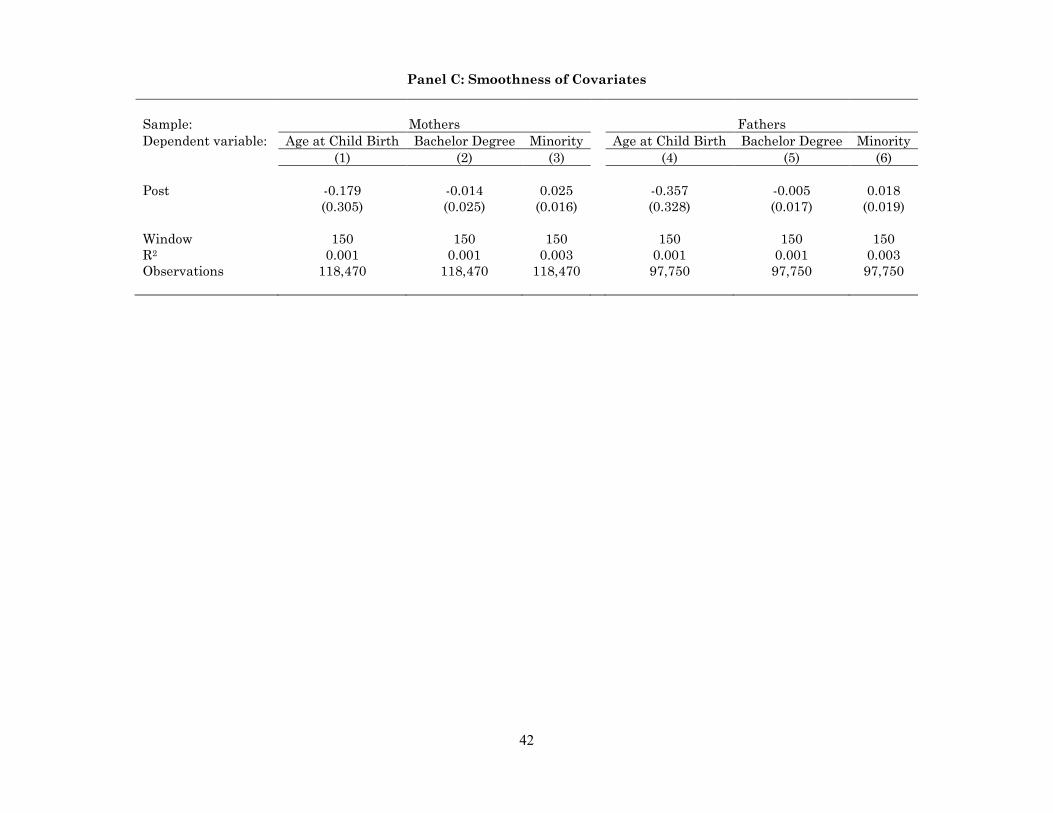
42

Panel C: Smoothness of Covariates

Sample: Mothers Fathers Dependent variable: Age at Child Birth Bachelor Degree Minority Age at Child Birth Bachelor Degree Minority (1) (2) (3) (4) (5) (6) Post -0.179 -0.014 0.025 -0.357 -0.005 0.018 (0.305) (0.025) (0.016) (0.328) (0.017) (0.019) Window 150 150 150 150 150 150 R2 0.001 0.001 0.003 0.001 0.001 0.003 Observations 118,470 118,470 118,470 97,750 97,750 97,750

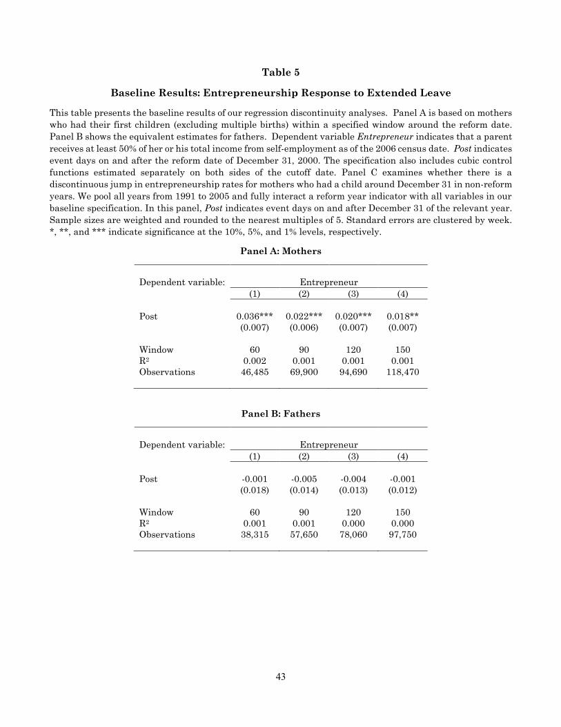
43

Table 5

Baseline Results: Entrepreneurship Response to Extended Leave

This table presents the baseline results of our regression discontinuity analyses. Panel A is based on mothers who had their first children (excluding multiple births) within a specified window around the reform date. Panel B shows the equivalent estimates for fathers. Dependent variable Entrepreneur indicates that a parent receives at least 50% of her or his total income from self-employment as of the 2006 census date. Post indicates event days on and after the reform date of December 31, 2000. The specification also includes cubic control functions estimated separately on both sides of the cutoff date. Panel C examines whether there is a discontinuous jump in entrepreneurship rates for mothers who had a child around December 31 in non-reform years. We pool all years from 1991 to 2005 and fully interact a reform year indicator with all variables in our baseline specification. In this panel, Post indicates event days on and after December 31 of the relevant year. Sample sizes are weighted and rounded to the nearest multiples of 5. Standard errors are clustered by week. *, **, and *** indicate significance at the 10%, 5%, and 1% levels, respectively.

Panel A: Mothers

Dependent variable: Entrepreneur (1) (2) (3) (4) Post 0.036*** 0.022*** 0.020*** 0.018** (0.007) (0.006) (0.007) (0.007) Window 60 90 120 150 R2 0.002 0.001 0.001 0.001 Observations 46,485 69,900 94,690 118,470

Panel B: Fathers

Dependent variable: Entrepreneur (1) (2) (3) (4) Post -0.001 -0.005 -0.004 -0.001 (0.018) (0.014) (0.013) (0.012) Window 60 90 120 150 R2 0.001 0.001 0.000 0.000 Observations 38,315 57,650 78,060 97,750

44

Panel C: Placebo Test in Non-Reform Years

Dependent variable: Entrepreneur (1) (2) (3) (4) Post 0.002 -0.001 -0.003 -0.003 (0.003) (0.005) (0.004) (0.004) Reform Year × Post 0.034*** 0.023*** 0.023*** 0.021*** (0.008) (0.008) (0.008) (0.008) Window 60 90 120 150 R2 0.001 0.000 0.000 0.000 Observations 781,610 1,179,580 1,597,780 2,006,615

45

Table 6

Robustness to Other Samples and Control Functions

This table presents the results of various robustness tests. Panel A estimates the discontinuity using a quartic rather than cubic polynomial as the control function. Panel B uses a local linear regression with an Epanechnikov kernel and various bandwidths as the control function. Panel C estimates our baseline specification including all children born in the estimation window. Dependent variable Entrepreneur indicates that a mother receives at least 50% of her total income from self-employment as of the 2006 census date. Post indicates event days on and after December 31, 2000. Sample sizes are weighted and rounded to the nearest multiples of 5. Standard errors are clustered by week. *, **, and *** indicate significance at the 10%, 5%, and 1% levels, respectively.

Panel A: Quartic Polynomial Dependent variable: Entrepreneur (1) (2) (3) (4) Post 0.031*** 0.030*** 0.021*** 0.020*** (0.007) (0.007) (0.007) (0.006) Window 60 90 120 150 R2 0.002 0.001 0.001 0.001 Observations 46,485 69,900 94,690 118,470

Panel B: Non-Parametric Dependent variable: Entrepreneur (1) (2) (3) (4) Post 0.022*** 0.026*** 0.029*** 0.026*** (0.003) (0.002) (0.003) (0.003) Window 150 150 150 150 Bandwidth 14 days 21 days 28 days 35 days Observations 118,470 118,470 118,470 118,470

Panel C: All Children Dependent variable: Entrepreneur (1) (2) (3) (4) Post 0.022** 0.013** 0.010** 0.012** (0.009) (0.006) (0.005) (0.005) Window 60 90 120 150 R2 0.000 0.000 0.000 0.000 Observations 101,965 153,615 209,085 262,865

46

Table 7

Heterogeneity in Entrepreneurship Response to Extended Leave Depending on Entrepreneur Characteristics

This table examines whether our main results differ across subsamples, i.e., those with and without a college degree (columns 1-2), those above and below the median age at child birth (columns 3-4), and those with a high income and low income spouse (columns 5-6). The samples are based on mothers who had a child within 5 months of the December 31, 2000 reform date. P-values indicates the significance of the differences in coefficient Post across subsamples. Sample sizes are weighted and rounded to the nearest multiples of 5. Standard errors are clustered by week. *, **, and *** indicate significance at the 10%, 5%, and 1% levels, respectively.

Subsample: BA Degree No BA Degree Age>=29 Age<29 High Income Spouse Low Income Spouse (1) (2) (3) (4) (5) (6) Post 0.046** -0.001 0.028*** -0.009 0.028** 0.000 (0.019) (0.006) (0.007) (0.006) (0.012) (0.007) Window 150 150 150 150 150 150 P-value 0.037 0.037 0.000 0.000 0.092 0.092 R2 0.001 0.000 0.000 0.001 0.001 0.000 Observations 69,725 193,140 143,780 119,085 112,645 150,220

47

Table 8

Entrepreneurship Quality

This table reports the results using various classifications of entrepreneurship. In Panel A, the dependent variable is an indicator equal to one if at least 50% of the mother’s total income comes from self-employment and she reports herself as self-employed. In Panel B, the dependent variable is an indicator equal to one if at least 50% of the mother’s income comes from self-employment and she reports herself as being self-employed with paid employees. Panel C is similar but without paid employees. The samples are based on mothers who had a child within 5 months of the December 31, 2000 reform date. Sample sizes are weighted and rounded to the nearest multiples of 5. Standard errors are clustered by week. *, **, and *** indicate significance at the 10%, 5%, and 1% levels, respectively.

Panel A: Report Entrepreneurship Dependent variable: Entrepreneur (Self-Reported) (1) (2) (3) (4) Post 0.013*** 0.007* 0.007** 0.008** (0.003) (0.004) (0.003) (0.003) Window 60 90 120 150 R2 0.000 0.000 0.000 0.000 Observations 101,965 153,615 209,085 262,865

Panel B: Entrepreneur with Paid Employees Dependent variable: Entrepreneur With Paid Employees (1) (2) (3) (4) Post 0.008*** 0.005*** 0.004** 0.006*** (0.003) (0.002) (0.002) (0.002) Window 60 90 120 150 R2 0.000 0.000 0.000 0.000 Observations 101,965 153,615 209,085 262,865

Panel C: Entrepreneur without Paid Employees Dependent variable: Entrepreneur Without Paid Employees (1) (2) (3) (4) Post 0.005* 0.002 0.002 0.002 (0.002) (0.003) (0.003) (0.003) Window 60 90 120 150 R2 0.000 0.000 0.000 0.000 Observations 101,965 153,615 209,085 262,865

48

Table 9

High Startup Capital vs Low Startup Capital

This table examines whether our main results differ for entrepreneurs entering into industries with different levels of startup capital. Following Adelino et al. (2015), we obtain information on industry level startup capital from the Survey of Business Owners (SBO) Public Use Microdata Sample (PUMS) by selecting the sample of new firms in each industry and averaging the amount of capital needed to start those firms. High startup capital is defined as 2-digit NAICS industries for which the amount of startup capital is higher than the median for all industries. In Panel A, the dependent variable is an indicator equal to one if at least 50% of the mother’s total income comes from self-employment and she report being in an industry with high startup capital requirements. Panel B is similar but the dependent variable only includes entrepreneurs in industries with startup capital requirements below the median. The samples are based on mothers who had a child within 5 months of the December 31, 2000 reform date. Sample sizes are weighted and rounded to the nearest multiples of 5. Standard errors are clustered by week. *, **, and *** indicate significance at the 10%, 5%, and 1% levels, respectively.

Panel A: Entrepreneur in High Startup Capital Industries Dependent variable: Entrepreneur in High Startup Capital Industries (1) (2) (3) (4) Post 0.024*** 0.019*** 0.008** 0.006 (0.005) (0.003) (0.004) (0.004) Window 60 90 120 150 R2 0.001 0.001 0.000 0.000 Observations 101,965 153,615 209,085 262,865

Panel B: Entrepreneur in Low Startup Capital Industries Dependent variable: Entrepreneur in Low Startup Capital Industries (1) (2) (3) (4) Post -0.002 -0.006 0.002 0.006 (0.007) (0.004) (0.005) (0.006) Window 60 90 120 150 R2 0.001 0.000 0.000 0.000 Observations 101,965 153,615 209,085 262,865

49

Table 10

High Startup Risk vs Low Startup Risk

This table examines whether our main results differ for entrepreneurs entering into industries with different levels of startup risk. We compute two industry-level measures of startup risk based on complete UK private firm data provided by Bureau van Dijk’s Orbis database. For each 3-digit NAICS industry, we first compute the exit rate among new firms within the first five years of incorporation. We also compute average 5-year cash flow volatility among young firms less than 10 years old. High startup risk industries are defined as industries for which the exit rate or the cash flow volatility is higher than the median for all industries. In Panels A and C, the dependent variable is an indicator equal to one if at least 50% of the mother’s total income comes from self-employment and she report being in a high startup risk industry. Panels B and D are similar but the dependent variable only includes entrepreneurs in industries with below median startup risk. The samples are based on mothers who had a child within 5 months of the December 31, 2000 reform date. Sample sizes are weighted and rounded to the nearest multiples of 5. Standard errors are clustered by week. *, **, and *** indicate significance at the 10%, 5%, and 1% levels, respectively.

Panel A: Entrepreneur in High Exit Rate Industries Dependent variable: Entrepreneur in High Exit Rate Industries (1) (2) (3) (4) Post 0.027*** 0.018*** 0.011*** 0.011*** (0.006) (0.006) (0.004) (0.004) Window 60 90 120 150 R2 0.001 0.001 0.000 0.000 Observations 101,965 153,615 209,085 262,865

Panel B: Entrepreneur in Low Exit Rate Industries Dependent variable: Entrepreneur in Low Exit Rate Industries (1) (2) (3) (4) Post -0.005 -0.005 -0.001 0.001 (0.004) (0.003) (0.004) (0.004) Window 60 90 120 150 R2 0.000 0.000 0.000 0.000 Observations 101,965 153,615 209,085 262,865

50

Panel C: Entrepreneur in High Cash Flow Volatility Industries Dependent variable: Entrepreneur in High Cash Flow Volatility Industries (1) (2) (3) (4) Post 0.024*** 0.017*** 0.009** 0.010** (0.005) (0.005) (0.004) (0.004) Window 60 90 120 150 R2 0.001 0.001 0.000 0.000 Observations 101,965 153,615 209,085 262,865

Panel D: Entrepreneur in Low Cash Flow Volatility Industries Dependent variable: Entrepreneur in Low Cash Flow Volatility Industries (1) (2) (3) (4) Post -0.002 -0.004 0.001 0.002 (0.004) (0.003) (0.004) (0.004) Window 60 90 120 150 R2 0.000 0.000 0.000 0.000 Observations 101,965 153,615 209,085 262,865

Appendix

[For Online Publication]

A Quantifying Worst-Case Selection Bias

Although Table 4 showed no significant differences in the number of births on either side of thediscontinuity, or in the predetermined characteristics of the mothers, the probative value of thesefacts is limited by the power of the estimates. In this appendix, we quantify the potential bias inour main estimates while accounting for the estimation error in Table’s 4 validity checks.

To think formally about this bias, suppose that there are two groups in the population, thosewith a high probability (pH) of becoming entrepreneurs and those with a low probability (pL). Let✓ be the share of H-types in the population, and let subscripts 0 and 1 index the periods beforeand after the policy change. So prior to the change, the share of entrepreneurs in the populationis (1 � ✓0)pL0 + ✓0p

H0 . If the policy has a treatment effect then the self-employment probabilities

change for a given type of person, so pH1 > pH0 or pL1 > pL0 . If the policy does not have a treatmenteffect, then we could still estimate an apparent treatment effect if the population changes, that is✓1 > ✓0. The observed share of entrepreneurs after the policy change is (1� ✓1)pL1 + ✓1p

H1 .

In order to test whether our results are driven by selection, we will assume that the policy hasno treatment effect so pH1 = pH0 = pH and pL1 = pL0 = pL. Thus the difference in the share ofentrepreneurs we observe is

(1� ✓1)pL + ✓1p

H � (1� ✓0)pL � ✓0p

H = (✓1 � ✓0)pH � (✓1 � ✓0)p

L = �✓ ·�p (5)

where �✓ = ✓1 � ✓0 and �p = pH � pL. Note that the difference operator on the population shares✓ refers to the change across the time periods, while the difference operator on the probabilitiesrefers to theH-types’ additional propensity to become entrepreneurs (in the cross-section). Weaim to determine the largest value that this product could plausibly take, and that will provide aconservative estimate of how much selection bias our main estimates might suffer.

Empirically we do not observe whether a mother has type H or type L. So we proxy for thiswith her observable predetermined characteristics. We first run a purely observational regressionof entrepreneurship probability on the same cross-sectional characteristics we examined in Table 4,namely age, education, and ethnicity:

yit = ⇣1Ageit + ⇣2Educationit + ⇣3Minorityit + ✏it. (6)

The estimated coefficients ⇣ serve a role analogous to �p in equation (5). Changes in the age,education and minority status across the discontinuity, as seen in Panel C of Table 4, play a roleanalogous to �✓. Let X = (Aget, Educationt,Minorityt) be the vector of average characteristics inthe population at time t, namely on either side of the discontinuity. Then the inner product ⇣ ·�Xallows us to gauge how much selection bias (on observables) could drive our results.

Table A2 presents the results from estimating a few variants of equation (6). A first observationis that the direction of the point estimates actually suggests bias opposite to the direction of ourmain results. Older and more educated mothers are more likely to be entrepreneurs. But the pointestimates for �X, from Panel C of Table 4, shows that their share falls after the policy change. Soan estimate of ⇣ ·�X based on the point estimates implies a bias opposite to the results we actuallyobserve, and specifically of -0.001.

Although these point estimates suggest that selection is unlikely to explain our results, we go one

step further and consider the worst case selection bias consistent with the mothers’ characteristics weobserve. That is, we consider the 95 percent confidence interval of the changes in each demographicvariable in X, and focus on values in those intervals that would maximize the bias in the direction ofour results.16 Since age and education are associated with higher entrepreneurship, we consider thetop of Table 4’s confidence intervals for those two variables, namely an age of 0.42 years older and a3.5 percentage point increase in the share of college graduates. Since minority status is associatedwith lower entrepreneurship, the bias in favor of our results would be maximized at the bottomof the confidence interval, or a change of -0.006 in the minority share. Putting these variablestogether, we find a maximum selection bias of ⇣ ·�X = 0.002. Thus the worst case bias is an orderof magnitude smaller than our estimated treatment effects in Table 5.

Table A3 presents a conceptually similar exercise, in which we look for a discontinuity in pre-dicted entrepreneurship based on individual covariates. We first estimate a regression to predictentrepreneurship based on the covariates included in equation (6), plus their interactions. Usingthose estimates, we compute the predicted probability of entrepreneurship for each mother in ourdata. We then estimate our baseline regression, equation (3), with the predicted entrepreneurshippropensity as the dependent variable. Table A3 shows these estimates. The coefficients indicatethat those eligible for longer leave are, if anything, less likely to be entrepreneurs than those whogave birth before the discontinuity. This difference is significant in column 2, but otherwise in-distinguishable from zero. So these results confirm our previous calculation: selection bias cannotgenerate our main finding.

16Because our estimates of how these variables relate to entrepreneurship probabilities, ⇣, are extremely precise,we do not concern ourselves with estimation error in ⇣.

Appendix TablesTable A1. Baseline Results: Replication on Data Collapsed to Day Level

This table repeats our baseline regression discontinuity estimates on daily level data. We take the samples from Table 5 Panel A and collapse them to the day-level. The dependent variable Entrepreneurship Rate is the fraction of mothers giving birth on an event day who receive at least 50% of their total income from self-employment as of the 2006 census date. Post indicates event days on and after the reform date of December 31, 2000. The specification includes cubic time trends on both sides of the cutoff date. Sample sizes correspond to the number of days in the estimation windows. Each observation is weighted by the number of births on that day. Standard errors are clustered by week. *, **, and *** indicate significance at the 10%, 5%, and 1% levels, respectively.

Dependent variable: Entrepreneurship Rate (1) (2) (3) (4) Post 0.036*** 0.022*** 0.020*** 0.018** (0.008) (0.006) (0.007) (0.007) Window 60 90 120 150 R2 0.002 0.001 0.001 0.001 Number of days 121 181 241 301

Table A2. Entrepreneurship and Cross-Sectional Characteristics

This table presents the cross-sectional relationship between mothers’ entrepreneurship probability and their predetermined characteristics examined in Table 4 Panel C. Dependent variable Entrepreneur indicates that a mother receives at least 50% of her total income from self-employment as of the 2006 census date. Samples are the same as those used in columns 1 to 3 of Table 4 Panel C. Standard errors are clustered by week of child birth. *, **, and *** indicate significance at the 10%, 5%, and 1% levels, respectively.

Dependent variable: Entrepreneur (1) (2) (3) (4)

Age at Child Birth 0.003*** 0.003***

(0.000) (0.000) Bachelor Degree 0.019*** 0.011***

(0.004) (0.004) Minority -0.022*** -0.021***

(0.003) (0.003)

Window 150 150 150 150 R2 0.006 0.002 0.002 0.009 Observations 118,470 118,470 118,470 118,470

Table A3. Discontinuity in Predicted Entrepreneurship Propensity

This table re-estimate an analogue of our baseline specification, where the dependent variable is changed to the predicted propensity to be an entrepreneur. This propensity is estimated through a regression of self-employment against a variety of individual characteristics and their interactions. Other than the change in the dependent variable, the specification follows that used in Table 5 Panel A. Sample sizes are weighted and rounded to the nearest multiples of 5. Standard errors are clustered by week. *, **, and *** indicate significance at the 10%, 5%, and 1% levels, respectively.

Dependent variable: Predicted Entrepreneurship from Covariates (1) (2) (3) (4) Post -0.001 -0.002* -0.001 -0.001 (0.001) (0.001) (0.001) (0.001) Window 60 90 120 150 R2 0.002 0.001 0.001 0.001 Observations 46,485 69,900 94,690 118,470 Number of days 121 181 241 301

Table A4. Job-Protected Leave vs Paid Leave

This table re-estimate our baseline specification limiting to mothers that gave birth in Quebec, where job-protected leave did not increase but paid leave increased during the 2001 reform. The specification follows that used in Table 5 Panel A. Sample sizes are weighted and rounded to the nearest multiples of 5. Standard errors are clustered by week. *, **, and *** indicate significance at the 10%, 5%, and 1% levels, respectively.

Dependent variable: Entrepreneur (1) (2) (3) (4) Post 0.006 -0.006 -0.007 0.025 (0.014) (0.033) (0.027) (0.026) Window 60 90 120 150 R2 0.009 0.005 0.005 0.003 Observations 10,000 15,130 20,470 25,725