i

Experimental Testing and Modelling of Adhesively

Joined T-structures

by

Khaled Boqaileh

A thesis

presented to the University of Waterloo

in fulfillment of the

thesis requirement for the degree of

Master of Applied Science

in

Mechanical Engineering

Waterloo, Ontario, Canada, 2015

© Khaled Boqaileh 2015

ii

AUTHOR'S DECLARATION

I hereby declare that I am the sole author of this thesis. This is a true copy of the thesis, including any

required final revisions, as accepted by my examiners.

I understand that my thesis may be made electronically available to the public.

Khaled Boqaileh

iii

ABSTRACT

As fuel-efficiency standards continue to push original equipment manufacturers (OEM's) to produce more

fuel-efficient vehicles, it is important to look at new and innovative ways to achieve this goal. Although

there are multiple solutions to this challenge including powertrain refinement and aerodynamics, a

primary focus is to reduce the weight of vehicles. To achieve this goal the designers can utilize

combinations of high strength and lightweight materials to reduce vehicle structure weight. The main

challenge that arises when joining mixed materials using conventional methods such as welding or

mechanical fasteners is galvanic corrosion. This form of corrosion occurs when two dissimilar materials

are in contact over time. Furthermore, dissimilar materials often cannot be joined using traditional

methods such as welding. Adhesives provide a solution to this challenge, providing a barrier between the

two materials to mitigate galvanic corrosion. Additionally, adhesives can provide improved NVH (noise,

vibration and harshness) performance and create a more evenly distributed stresses within the joint. With

increasing interest in adhesives for joining materials, it has become important for designers to have

accurate material models to use in finite element simulations for design and optimization.

The goal of this thesis was to evaluate the feasibility of applying bulk material and coupon-level test data

to predict structural response and failure under quasi-static and dynamic conditions. Two commercial

toughened structural epoxy adhesives were investigated (DP460NS and SA9850, 3M Company,

Minnesota) to join structures subject to quasi-static and dynamic load levels.

Structural testing was undertaken on T-shaped samples created by adhesively joining two Al6063-T5 C-

channels. For each adhesive, four structural experimental tests were undertaken including quasi-static

direct shear (2.5 mm/min), quasi-static torsion (2.5 mm/min), unsupported dynamic impact shear

(4.43 m/s) and supported dynamic impact shear (3.96 m/s).

Surface preparation is an important component when assessing the strength of the adhesive. Grit blasting

was used to prepare the surfaces of the DP460NS samples since this was previously demonstrated to

provide good bond strength with low variability. The second adhesive (SA9850) was tested with two

surface preparations, grit blasting and with forming lubricant applied to the surface, where the forming

lubricant surface contamination provided higher strength and lower variability. In general, the four

experimental tests demonstrated consistent responses concerning shape, maximum force and

displacement at failure. In addition, it was found that the dynamic impact forces at failure were larger

than the quasi-static forces at failure. This result was expected because both adhesives were strain rate

dependent.

iv

Numerical models of the experiments were developed using adhesive mechanical properties determined

in previous studies from bulk and coupon-level tests, and integrated into a cohesive element formulation.

A boundary condition sensitivity study was undertaken, guided by imaging acquired during the

experimental testing. The final models comprised C-channels modeled with solid elements, adhesive

modeled with cohesive elements, and a detailed model of the experimental fixture to account for fixture

compliance during the test. The aluminum C-channels were modeled using an incremental plasticity

model with a von Mises yield surface. It was determined that deformation rate effects were significant for

the adhesive and a rate-dependent cohesive model was implemented to address this challenge. Lastly, a

mesh convergence study was carried out and resulted in a convergence at an element size of 2mm.

The numerical simulation results for the SA9850 adhesive were in good agreement with the experiments

for all four load cases, demonstrated by an excellent cross correlation rating. Similar results were

obtained for the DP460NS, with the exception of the quasi-static torsion case, where the numerical model

underpredicted the force and displacement at failure. This was attributed to the constitutive model not

accounting from Mode III material properties, the mode of loading for this test case, which can differ

significantly from Mode II for some adhesives.

In general, the failure forces predicted in the numerical simulations were lower than the average

experimental force, which was also proven through statistical analysis. This issue was attributed to the

source of the shear data for the material models, which was a thick adherend lap shear. The shear data

used for the material model development included a relatively thick bond line, which is known to affect

the measured strength properties. Additionally, the thick adherend lap shear test does not result in pure

shear data. It is recommended that further testing be undertaken to measure shear properties to be used in

future modeling efforts.

Fatigue testing was also carried out on the two adhesives. The testing was done with a tensile test sample,

single lap shear sample and a structural test sample. The S-N curve measured with tensile test samples

was log-linear. However, the single lap shear fatigue testing revealed that at lower stress amplitudes the

effects of the bending of the adherend caused early failure of the joint and in many cases resulted in

failure of the adherend and not the adhesive, emphasizing the importance of joint design. Fatigue testing

on the T-structure demonstrated a similar curve shape when compared to the single lap shear testing with

the primary difference being that the structural tests resulted in fewer cycles to failure at the same stress

amplitude. This difference can be attributed to the larger adhesion area in the structural sample when

v

compared to the single lap shear sample, and therefore a higher likelihood of defects in the joint that

could initiate fatigue failure.

The main goal of this thesis was to verify the applicability of a cohesive approach to model structural

response. In general, the model results demonstrated that material properties measured at the bulk and

coupon levels can accurately predict the response and failure of an adhesive joint in a structural test.

vi

ACKNOWLEDGEMENTS

I acknowledge all those that helped me, of whom there are many. I would like to thank Luis Fernando

Trimiño Rincon, Jeff Wemp and Yogi Nandwani who were instrumental in completing this thesis. I

would lastly like to especially thank Duane Cronin, who made this thesis possible.

I would like to thank Mary M. Caruso-Dailey and Kent Nielsen of 3M Company, Initiative for Advanced

Manufacturing Innovation and Automotive Partnerships Canada for financially supporting this research. I

would also like thank Compute Canada for providing the necessary computing resources.

vii

DEDICATION

This is dedicated to my family without whom I would not be where I am today. I would like to especially

thank my father and mother, two of the most supportive people in my life.

viii

TABLE OF CONTENTS

AUTHOR'S DECLARATION ...................................................................................................................... ii

ABSTRACT ................................................................................................................................................. iii

ACKNOWLEDGEMENTS ......................................................................................................................... vi

DEDICATION ............................................................................................................................................ vii

TABLE OF CONTENTS ........................................................................................................................... viii

LIST OF TABLES ...................................................................................................................................... xii

LIST OF FIGURES ................................................................................................................................... xiv

LIST OF EQUATIONS ........................................................................................................................... xviii

NOMENCLATURE .................................................................................................................................. xix

Chapter 1 : INTRODUCTION .................................................................................................................. 1

1.1 RESEARCH MOTIVATION ....................................................................................................... 1

1.2 RESEARCH APPROACH AND OBJECTIVES ......................................................................... 7

Chapter 2 : BACKGROUND .................................................................................................................... 8

2.1 ADHESIVES ................................................................................................................................ 8

2.1.1 EPOXY ADHESIVE ............................................................................................................ 8

2.1.2 FAILURE MODES: INTERFACIAL AND COHESIVE .................................................. 11

2.1.3 SURFACE PREPARATION .............................................................................................. 12

2.2 ADHESIVE MATERIAL PROPERTIES .................................................................................. 14

2.2.1 SHEAR TESTING .............................................................................................................. 15

2.2.2 CLEAVAGE TEST............................................................................................................. 18

2.2.3 TENSILE TEST .................................................................................................................. 19

2.3 DATA EVALUATION............................................................................................................... 22

2.4 STRUCTURAL TESTING ......................................................................................................... 23

2.5 FATIGUE TESTING .................................................................................................................. 24

ix

2.6 NUMERICAL SIMULATION OF ADHESIVES ...................................................................... 25

2.6.1 FEA AND FEM BACKGROUND ..................................................................................... 25

2.6.2 IMPLICIT OR EXPLICIT .................................................................................................. 27

2.6.3 MATERIAL MODELS ....................................................................................................... 28

2.6.4 COHESIVE ZONE MODEL .............................................................................................. 29

Chapter 3 : METHODS ........................................................................................................................... 35

3.1 EXPERIMENTAL STRUCTURAL TESTING ......................................................................... 35

3.1.1 STRUCTURAL SAMPLE DESIGN .................................................................................. 35

3.1.2 QUASI-STATIC DIRECT SHEAR TESTS ....................................................................... 36

3.1.3 QUASI-STATIC TORSIONAL SHEAR TESTS ............................................................... 37

3.1.4 DYNAMIC IMPACT TESTS ............................................................................................. 37

3.2 NUMERICAL SIMULATION ................................................................................................... 40

3.2.1 COHESIVE MODEL MATERIAL PARAMATERS ........................................................ 41

3.2.2 SINGLE ELEMENT VERIFICATION .............................................................................. 42

3.2.3 ADHESIVE MESH CONVERGENCE STUDY ................................................................ 47

3.2.4 ALUMINUM C-CHANNELS MATERIAL PROPERTIES .............................................. 48

3.2.5 BOUNDARY CONDITIONS ............................................................................................. 48

3.3 Fatigue testing ............................................................................................................................. 54

3.3.1 TENSILE SAMPLE FATIGUE TESTING ........................................................................ 56

3.3.2 SINGLE LAP SHEAR FATIGUE TESTING .................................................................... 56

3.3.3 STRUCTURAL SAMPLE FATIGUE TESTING .............................................................. 57

Chapter 4 : RESULTS AND DISCUSSIONS ........................................................................................ 58

4.1 : COMPARISON OF NUMERICAL AND EXPERIMENTAL RESULTS .............................. 58

4.1.1 QUASI-STATIC TESTING ............................................................................................... 58

4.1.2 TORSIONAL TESTING .................................................................................................... 65

4.1.3 DYNAMIC IMPACT ......................................................................................................... 69

4.1 FATIGUE TESTING RESULTS ................................................................................................ 80

x

4.1.1 DOG BONE FATIGUE RESULTS .................................................................................... 80

4.1.2 SINGLE LAP SHEAR FATIGUE RESULTS ................................................................... 80

4.1.3 STRUCTURAL SAMPLE FATIGUE RESULTS ............................................................. 82

Chapter 5 : SUMMARY AND RECOMMENDATIONS ....................................................................... 84

5.1 SUMMARY ................................................................................................................................ 84

5.2 RECOMMENDATIONS ............................................................................................................ 86

APPENDIX A: STRUCTURAL SAMPLE SPECIFICATIONS AND MANUFACTURING .................. 87

MECHANICAL DRAWINGS ............................................................................................................... 87

MANUFACTURING PROCES FOR STRUCTURAL TEST SAMPLES ............................................ 91

APPENDIX B: FATIGUE SAMPLE SPECIFICATIONS......................................................................... 93

APPENDIX C: TEST MACHINE DETAILS ............................................................................................ 94

5.1 Quasi-static shear, torsion and fatigue single lap shear test rig .................................................. 94

5.2 Tensile test sample fatigue test rig .............................................................................................. 95

5.3 Dynamic impact test rig .............................................................................................................. 97

APPENDIX D: FIXTURE EVOLUTION .................................................................................................. 98

APPENDIX E: TESTING FIXTURES ..................................................................................................... 100

APPENDIX F: MESH CONVERGENCE ANALYSIS ........................................................................... 104

APPENDIX G: LS-DYNA CARDS ......................................................................................................... 106

APPENDIX H: NUMERICAL SIMULATION EVOLUTION ............................................................... 113

QUASI STATIC SHEAR ..................................................................................................................... 113

SUPPORTED DYNAMIC IMPACT TEST ......................................................................................... 115

UNSUPPORTED DYNAMIC IMPACT TEST ................................................................................... 117

APPENDIX I: EXPERIMENTAL RESULTS COMPARING HCF AND LCF AND SURFACE

PREPERATION ....................................................................................................................................... 119

DP460NS QUASI-STATIC DIRECT SHEAR EXPERIMENTAL RESULTS................................... 119

SA9850 QUASI-STATIC DIRECT SHEAR EXPERIMENTAL RESULTS ...................................... 121

DP460NS TORSION EXPERIMENTAL RESULTS .......................................................................... 125

xi

SA9850 TORSION EXPERIMENTAL RESULTS ............................................................................. 126

DP460NS DYNAMIC IMPACT EXPERIMENTAL RESULTS ........................................................ 127

SA9850 DYNAMIC IMPACT EXPERIMENTAL RESULTS ........................................................... 129

SA9850 SURFACE PREPARATION CONCLUSION ....................................................................... 132

APPENDIX J: STRAIN RATE AFFECTS ON THE NUMERICAL SIMULATION ............................ 133

REFERENCES ......................................................................................................................................... 135

xii

LIST OF TABLES

Table 1: Ford F150 and Range Rover Land Rover fuel economy figures [11] ............................................ 5

Table 2: DP460NS Properties at Quasi-static 0.05/s [25] ........................................................................... 10

Table 3: SA9850 Properties Quasi-static 0.1/s [25] .................................................................................... 11

Table 4: Summary of adhesive characterization tests ................................................................................. 14

Table 5: Tiebreak vs. cohesive zone model [66] vs. continuum models .................................................... 28

Table 6: Dynamic Impact testing specifications ......................................................................................... 38

Table 7: Cohesive vs continuum elements time to completion ................................................................... 41

Table 8: Simulation model parameters for cohesive elements .................................................................... 42

Table 9: DP460NS energy release rate in Mode II original and calculated ................................................ 43

Table 10: Al6063-T5 material properties [78] ............................................................................................ 48

Table 11: Impact velocity for unsupported dynamic impact ...................................................................... 52

Table 12: Impact velocity for supported dynamic impact .......................................................................... 53

Table 13: S-N curve testing percentages ..................................................................................................... 56

Table 14: Quasi-static shear experimental and numerical horizontal C-channel deformation comparison 60

Table 15: DP460NS quasi-static shear numerical simulation vs. experimental tests displacement, force

and energy comparison ............................................................................................................................... 61

Table 16 DP460NS Quasi-static shear – Cross correlation and size........................................................... 62

Table 17: SA9850 quasi-static shear numerical simulation vs. experimental testsdisplacement, force and

energy comparison ...................................................................................................................................... 64

Table 18: SA9850 Quasi-static shear – Cross correlation and size ............................................................ 65

Table 19:DP460NS quasi-static torsionnumerical simulation vs. experimental testsforce and energy

comparison .................................................................................................................................................. 66

Table 20: DP460NS Quasi-static torsion – Cross correlation and size ....................................................... 67

Table 21 : SA9850quasi-static torsionnumerical simulation vs. experimental testsforce and energy

comparison .................................................................................................................................................. 68

Table 22: SA9850 Quasi-static torsion – Cross correlation and size .......................................................... 69

Table 23: Unsupported dynamic impact experimental and numerical horizontal C-channel deformation

comparison .................................................................................................................................................. 71

Table 24: DP460NS Unsupported dynamic impact numerical simulation vs. experimental tests

displacement and energy comparison ......................................................................................................... 72

Table 25: DP460NS unsupported dynamic impact - Cross correlation and size ........................................ 73

Table 26: SA9850 Unsupported dynamic impact numerical simulation vs. experimental test displacement

and energy comparison ............................................................................................................................... 74

xiii

Table 27: SA9850 unsupported dynamic impact - Cross correlation and size ........................................... 75

Table 28: DP460NS supported dynamic impact numerical simulation vs. experimental tests displacement,

force and energy comparison ...................................................................................................................... 76

Table 29: DP460NS supported dynamic impact - Cross correlation and size ............................................ 77

Table 30: SA9850 supported dynamic impact tnumerical simulation vs. experimental tests displacement,

force and energy comparison ...................................................................................................................... 78

Table 31: SA9850 supported dynamic impact - Cross correlation and size ............................................... 79

Table 32: Statistical analysis of DP460NS – HCF vs. NCF ..................................................................... 121

Table 33: Statistical analysis of SA9850 with a contaminated surface – HCF vs. LCF ........................... 122

Table 34: SA9850 LCF grit blasted vs. contaminated surface experimental test results .......................... 124

Table 35: Statistical analysis of DP460NS ............................................................................................... 125

Table 36: Statistical analysis of SA9850 grit blasted and contaminated surface ...................................... 126

xiv

LIST OF FIGURES

Figure 1: Fuel economy standards for new passenger vehicles by country [1] ............................................ 1

Figure 2: Average US automobile fuel economy over time based on [3] ..................................................... 2

Figure 3: EU automobile CO2 emissions vs. time [6] ................................................................................... 2

Figure 4: Hybrid car sales over the last 10 years [7]..................................................................................... 3

Figure 5: Lamborghini Aventador multi-material body structure [9] ........................................................... 4

Figure 6: Honda accord weight vs. time [11] ................................................................................................ 5

Figure 7: Honda accord fuel economy vs. time [11] ..................................................................................... 5

Figure 8: Break down of materials used in the Audi A6BIW [12] ............................................................... 6

Figure 9: Adhesive test chain ........................................................................................................................ 7

Figure 10: Toughened epoxy macro picture – Magnification x 7500 [21] ................................................... 9

Figure 11: Mixing tube (left) Adhesive gun (Right) ................................................................................... 10

Figure 12: Interfacial vs. cohesive failure [29] ........................................................................................... 12

Figure 13: DP460NS Single lap shear surface preparation comparison [31] ............................................. 13

Figure 14: SA9850 Single lap shear surface preparation comparison [31] ................................................. 13

Figure 15: Types of joint stresses [33] ........................................................................................................ 14

Figure 16: Modes of loading (a) Mode I – opening (b) Mode II – In-plane shear (c) Mode III – Out of-

plane shear[37] ............................................................................................................................................ 15

Figure 17: Thin single lap shear adherend bending [40]............................................................................. 15

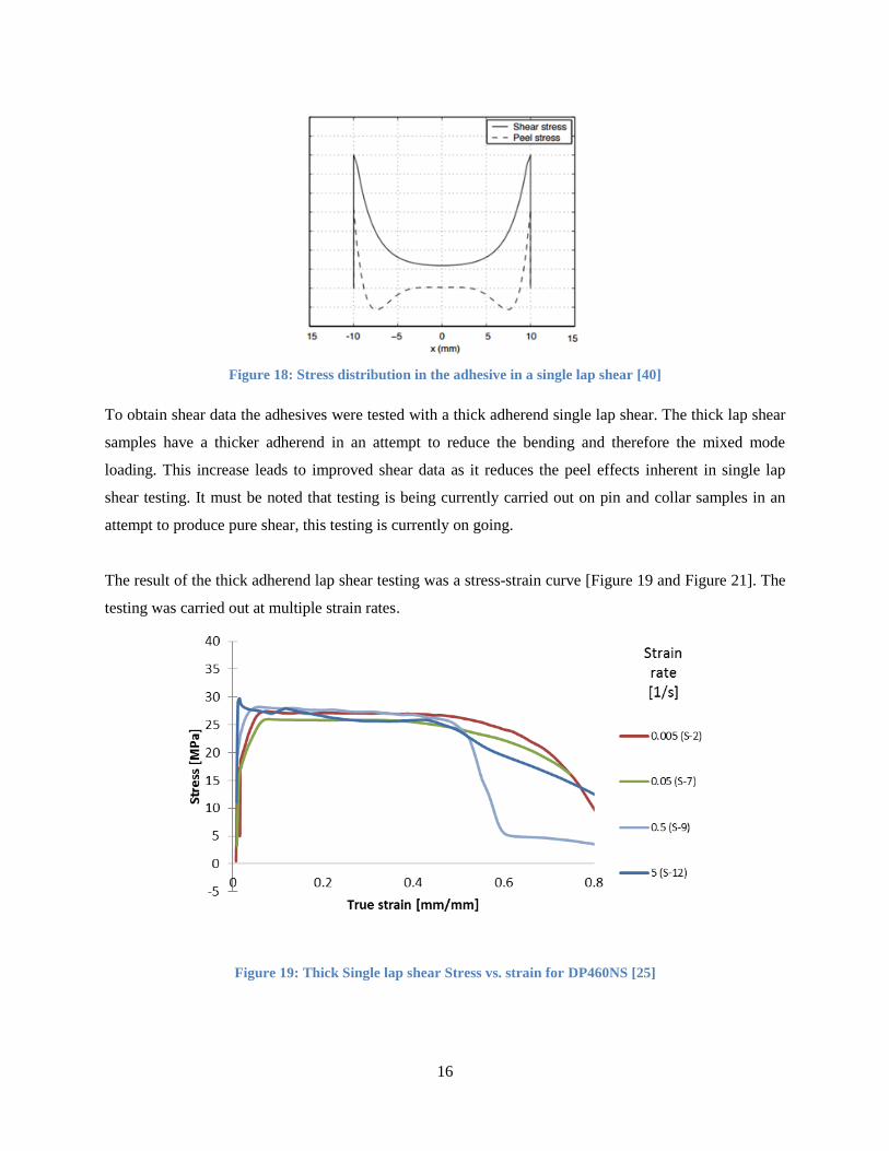
Figure 18: Stress distribution in the adhesive in a single lap shear [40] ..................................................... 16

Figure 19: Thick Single lap shear Stress vs. strain for DP460NS [25] ....................................................... 16

Figure 20: Stress at Failure vs. strain rate for DP460NS in shear [25] ....................................................... 17

Figure 21: Single lap shear Stress vs. strain for SA9850 [25] .................................................................... 17

Figure 22: Stress at Failure vs. strain rate for SA9850 in shear [25] .......................................................... 18

Figure 23: Double cantilever beam test [42] ............................................................................................... 19

Figure 24: Tensile test sample – Mini dogbone .......................................................................................... 19

Figure 25: comparison of ASTM tensile test sample and mini dogbone sample with DP460NS [25] ....... 20

Figure 26: Stress vs. strain DP460NS in tension [25] ................................................................................. 20

Figure 27: Stress at failure vs. strain rate for DP460NS in tension [25] ..................................................... 21

Figure 28: Stress vs. strain SA9850 in tension [25] .................................................................................... 21

Figure 29: Stress at failure vs. strain rate for SA9850 in tension [25] ........................................................ 22

Figure 30: T-sample highlighting shear and peel flanges [47] ................................................................... 23

Figure 31: Riveted T-shaped C-channels [48] ............................................................................................ 24

Figure 32: Preprocessing mesh example in 2D ........................................................................................... 26

xv

Figure 33: Preprocessing mesh example in 3D of tensile test sample ........................................................ 26

Figure 34: Continuum mechanics vs. cohesive zone model [67] ................................................................ 29

Figure 35: Evolution of the separation in the traction-separation curve ..................................................... 30

Figure 36: Traction-separation curve example ........................................................................................... 31

Figure 37: Traction-seperation curve details [66] ....................................................................................... 31

Figure 38: Mixed-mode Traction-seperation curve[66] .............................................................................. 33

Figure 39: Trilinear traction-separation law material number 240 [66] ...................................................... 34

Figure 40: Trilinear, mixed-mode traction-separation law [66] .................................................................. 34

Figure 41: Adhesively joined structural testing sample .............................................................................. 35

Figure 42: Quasi-static shear fixture (LCF) ................................................................................................ 36

Figure 43: Torsion fixture ........................................................................................................................... 37

Figure 44 : Dynamic impact unsupported fixture ....................................................................................... 38

Figure 45: Deformed sample in high deformation testing with no support ................................................ 39

Figure 46: Dynamic Impact with support ................................................................................................... 39

Figure 47: Flow chart for simulating adhesives .......................................................................................... 40

Figure 48: Single element cohesive simulation a) single element b) tension c) shear ................................ 42

Figure 49: DP460NS Single element in shear ............................................................................................ 44

Figure 50: SA9850 single element in shear ................................................................................................ 44

Figure 51: DP460NS single element in tension .......................................................................................... 45

Figure 52: SA9850 single element in tension ............................................................................................. 45

Figure 53: DP460NS thick adherend single lap shear numerical simulation vs. experimental test ............ 46

Figure 54: SA9850 thick adherend single lap shear numerical simulation vs. experimental test ............... 46

Figure 55: Simulation of thick adherend single lap shear ........................................................................... 47

Figure 56: Mesh convergence of energy absorbed ..................................................................................... 47

Figure 57: Securing bolt boundary condition for quasi-static shear ........................................................... 49

Figure 58: Quasi-static shear slight misalignment in the experiment (left) and in the simulation (right) .. 49

Figure 59: Quasi-static shear extended solid block simulation ................................................................... 50

Figure 60: Torsional simulation Securing bolts boundary condition .......................................................... 50

Figure 61: Torsional simulation moving bolt boundary condition ............................................................. 51

Figure 62: Components below the fixture (left) block representation of components (right) .................... 52

Figure 63: Unsupported boundary condition block (left) and bolts (right) ................................................. 53

Figure 64: Fixture and test sample unsupported (left) and supported (right) numerical simulation ........... 54

Figure 65: General tension-tension sine wave for fatigue testing ............................................................... 55

Figure 66: Tensile sample loaded in fatigue fixture.................................................................................... 56

xvi

Figure 67: Single lap shear - side view [50] ............................................................................................... 57

Figure 68: DP460NS quasi-static shear numerical simulation force-displacement result .......................... 59

Figure 69: Quasi static cohesive simulation – DP460NS – deformation before failure ............................. 59

Figure 70: Deformation of horizontal section during quasi-static shear testing - Numerical simulation

(left) and experimental test (right) .............................................................................................................. 60

Figure 71: DP460NS quasi-static shear numerical simulation vs. experimental tests ................................ 61

Figure 72: DP460NS Quasi-static shear - Experimental test 95% CI for displacement, force and Energy

compared to numerical simulation .............................................................................................................. 62

Figure 73: Spew fillet .................................................................................................................................. 63

Figure 74: SA9850 quasi-static shear numerical simulation vs. experimental tests ................................... 63

Figure 75: SA9850 Quasi-static shear - Experimental test 95% CI for displacement, force and Energy

compared to numerical simulation .............................................................................................................. 64

Figure 76: Quasi-static torsion simulation - start ........................................................................................ 65

Figure 77: DP460NS quasi-static torsionnumerical simulation vs. experimental tests .............................. 66

Figure 78: DP460NS Quasi-static torsion - Experimental test 95% CI for force and Energy compared to

numerical simulation ................................................................................................................................... 67

Figure 79: SA9850 quasi-static torsionnumerical simulation vs. experimental tests ................................. 68

Figure 80: SA9850 Quasi-static torsion - Experimental test 95% CI for force and Energy compared to

numerical simulation ................................................................................................................................... 69

Figure 81: Unsupported dynamic impact simulation before the test (left) and after the test (right) ........... 70

Figure 82: Unsupported dynamic impact numerical simulation (left) vs. experimental test (right) ........... 70

Figure 83: DP460NS Unsupported dynamic impact numerical simulation vs. experimental tests ............ 71

Figure 84: DP460NS unsupported dynamic impact - Experimental test 95% CI for force and Energy

compared to numerical simulation .............................................................................................................. 72

Figure 85: SA9850 Unsupported dynamic impact numerical simulation vs. experimental tests ................ 73

Figure 86: SA9850 unsupported dynamic impact - Experimental test 95% CI for force and Energy

compared to numerical simulation .............................................................................................................. 74

Figure 87: DP460NS dynamic impact with a supportnumerical simulation vs. experimental tests ........... 75

Figure 88: Supported dynamic impact simulation before the test (left) and after the test (right) ............... 76

Figure 89: DP460NS supported dynamic impact - Experimental test 95% CI for force and Energy

compared to numerical simulation .............................................................................................................. 77

Figure 90: SA9850 supported dynamic impact numerical simulation vs. experimental tests .................... 78

Figure 91: SA9850 supported dynamic impact - Experimental test 95% CI for force and Energy compared

to numerical simulation ............................................................................................................................... 79

xvii

Figure 92: Dog bone fatigue data S-N curve for DP460NS and SA9850 ................................................... 80

Figure 93: DP460NS and SA9850 percentage of maximum force vs. cycle’s to failure - Single lap shear

fatigue ......................................................................................................................................................... 81

Figure 94: Single lap shear bending during test .......................................................................................... 81

Figure 95: Stress distribution in the adhesive in a single lap shear example [40] ...................................... 82

Figure 96: Fatigue S-N curve for DP460NS single lap shear vs structural testing ..................................... 83

Figure 97: Horizontal channel with four holes (left), Vertical channel with one hole (left) ....................... 91

Figure 98: Fixture for creating the structural test samples .......................................................................... 92

Figure 99: High compliance quasi-static fixture - HCF .............................................................................. 98

Figure 100: Low compliance Quasi-static shear fixture - LCF ................................................................... 99

Figure 101: Dynamic impact initial fixture unsupported ............................................................................ 99

Figure 102: Mesh refinement from left to right (4mm, 2mm, 1mm, 0.2mm) ........................................... 104

Figure 103: Quasi-static– DP460NS - Shear - HCF ................................................................................. 119

Figure 104: Quasi-static – DP460NS - Shear - LCF ................................................................................. 120

Figure 105: Quasi-static – SA9850 - Shear - HCF ................................................................................... 121

Figure 106: Quasi-static – SA9850 - Shear – LCF – Grit blasted ............................................................ 122

Figure 107: Surface failure of SA9850 grit blasted - Interfacial failure (right) and cohesive failure (Left)

.................................................................................................................................................................. 123

Figure 108: SA9850 grit blasted - Horizontal section deformation comparison - Interfacial failure (right)

and cohesive failure (Left) ........................................................................................................................ 123

Figure 109: Spew fillet .............................................................................................................................. 124

Figure 110: Quasi-static SA9850 with a contaminated surface in Shear – LCF ....................................... 125

Figure 111: Quasi-static DP460NS torsion test results ............................................................................. 126

Figure 112: Quasi-static SA9850 with grit blast - torsion test results ...................................................... 127

Figure 113: Quasi-static SA9850 with contaminated surface- torsion test results ................................... 127

Figure 114: DP460NS unsupported dynamic impact test results .............................................................. 128

Figure 115: DP460NS supported dynamic impact test results .................................................................. 129

Figure 116: SA9850 grit blasted unsupporteddynamic impact test results ............................................... 130

Figure 117: SA9850 contaminated surface unsupported dynamic impact test results .............................. 130

Figure 118: SA9850 grit blasted unsupported dynamic impact test results .............................................. 131

Figure 119:SA9850 contaminated surface unsupported dynamic impact test results ............................... 131

Figure 120: SA9850 unsupported dynamic impact numerical simulation vs. experimental tests ............ 133

Figure 121: SA9850 supported dynamic impact numerical simulation vs. experimental tests ................ 134

xviii

LIST OF EQUATIONS

Equation 1: Cross correlation [45] .............................................................................................................. 22

Equation 2: Displacement to failure calculations[66] ................................................................................. 32

Equation 3: Mixed-mode loading displacement to failure[66] ................................................................... 32

Equation 4: Mixed-mode yield initiation displacement [66] ...................................................................... 34

Equation 5: Energy release rate in Mode II calculation [66] ...................................................................... 43

Equation 6: Fatigue Equations .................................................................................................................... 55

xix

NOMENCLATURE

FEA – Finite element analysis

FEM – Fining element Method

CAE – Computer aided engineering

BIW – Body in Weight

OEM – Original equipment manufacturer

DCB – Double cantilever beam

S-N curve – stress amplitudes vs. number of cycles to failure

CAD – Computer aided design

σ - Stress

MPa – Megapascals

Mpg – miles per gallon

CFD – Computational fluid dynamics

HCF – High compliance fixture

LCF – Low compliance fixture

NVH - Noise vibration harshness

CAFE (corporate average fuel economy)

UK - United Kingdom

US – United States

CI – Confidence Interval

LVDT - linear variable differential transformer

1

Chapter 1 : INTRODUCTION

1.1 RESEARCH MOTIVATION

The motivation to create more fuel-efficient vehicles is one that has come about primarily due to new

government regulations. These economy standards for fuel efficiency all around the world are increasing

each year [Figure 1].With these economy standards in mind, original equipment manufacturers (OEM’s)

have been forced to change how cars are designed to meet these new regulations.

Figure 1: Fuel economy standards for new passenger vehicles by country [1]

Such standards include the 2025 American standard in which the required fuel economy for cars and

light-duty trucks will be 54.5 miles per gallon (mpg) by 2025 [2]. This is a substantial increase in average

fuel economy because the current average is only 31.2 mpg [Figure 2]. This shows a large difference

between what is expected of car manufacturers by 2025 and what the current reality is. Therefore, many

new and innovative technologies will be required to increase the average fuel economy for vehicles.

2

Figure 2: Average US automobile fuel economy over time based on [3]

Another reason for creating cars that are more efficient is to address environmental issues. The negative

effect from car emissions has forced many governments around the world to introduce more stringent

emission laws. This was done in an effort to push car manufacturers to create vehicles that produce less

CO2, which has led to an increase in the amount of cars sold with lower CO2 emissions [Figure 3]. Some

of these regulations are the EU new car target [4] and the US CAFE (corporate average fuel economy)

standards [5]. Another reason for this decrease is due to the fact that in parts of the world such as the UK;

cars are taxed annually based on their annual emissions. Therefore, a lower emission vehicle is also

cheaper to own.

Figure 3: EU automobile CO2 emissions vs. time [6]

3

It can be seen that reducing the amount of fuel that a car uses is a positive step forward. To achieve this

goal there are three main aspects that can be reevaluated by OEMs.

The first way is for OEMs to refine and modify the powertrains to create vehicles that are more efficient.

This has meant a downsizing of engines, increased use of turbo charging, direct injection, higher

compression ratios and other means. Although these powertrain refinements are an important step

forward, many manufacturers have begun to put in more effort into producing hybrids and electric cars.

This change in powertrains has also meant that more hybrid and electric cars are being manufactured and

sold. [Figure 4]

Figure 4: Hybrid car sales over the last 10 years [7]

Another aspect that can be assessed to reduce fuel consumption is for the manufacturers to refine the

aerodynamics of vehicles. Although aerodynamics is not within the scope of this thesis it is also an

important part of creating vehicles that are more fuel-efficient. Simply put if a car can move through the

air more efficiently it will require less fuel [8].

The last aspect that OEMs can consider and the one this thesis will concentrate on is the goal to decrease

the mass of vehicles. The main way in which designers can decrease the mass of a vehicle is through

changing the materials that are used for many components. These material changes can be implemented to

the most fundamental parts of the car such as the chassis, doors, roofs etc. Currently, most vehicles are

designed using steel as the main material for all the major components. Although there has been a great

step forward in creating high strength steels, it has become important for designers to use other materials

such as aluminum, polymers, and composites to reduce mass. Supercars defined as “high performance

sports car”, have used alternative materials and manufacturing processes to reduce the weight of vehicles.

Although this use of mixed materials is mainly for performance purposes, one of the side effects is better

fuel economy. This use of exotic materials and manufacturing practices is only possible on supercars as

4

cost is not a consideration when compared to common consumer vehicles. Supercars show that through

the use of lighter materials vehicles can gain better fuel efficiency without sacrificing the safety or

comfort of the passengers. The vehicle shown is a Lamborghini Aventador [Figure 5], which through the

use of alternative materials can decrease weight while increasing performance and inadvertently

increasing fuel economy.

Figure 5: Lamborghini Aventador multi-material body structure [9]

Unlike supercars, the more common consumer vehicles have continued to increase in mass over time.

This is due to the fact that common consumer vehicles have continued to use similar materials for the

body in white (BIW) while adding more safety equipment, entertainment systems, luxury items and a

general increase in the size of the vehicles over time. All of these additions have resulted in a weight gain.

The graphs below show the changes in the Honda Accord attributes for the past 25 years. The weight of

the vehicle has increased [Figure 6] while the fuel economy has remained the same [Figure 7]. This

stagnation in fuel efficiency for vehicles can be attributed to this increase in mass. Although this graph

only shows the Honda Accord attributes, this trend is the same for all common consumer vehicles. To

address this trend, manufacturers have begun using aluminum to reduce the mass of vehicles [10]. The

Ford F150 and the Range Rover Land Rover are both vehicles that have recently seen a reduction of

732lbs and 926lbs respectively through the extensive use of aluminum. This decrease has also led to an

increase in the fuel efficiency of these two vehicles [Table 1].

5

Table 1: Ford F150 and Range Rover Land Rover fuel economy figures [11]

Previous combined

EPA (MPG)

New combined EPA

(MPG)

Increase (%)

Ford F150 18 22 18.2

Range Rover Land Rover 14 16 12.5

Figure 6: Honda accord weight vs. time [11]

Figure 7: Honda accord fuel economy vs. time [11]

While it is generally accepted that creating lighter vehicles is a positive step forward, OEMs have

multiple avenues to achieve this. The main way for OEMs to reduce mass is through the use of multi-

materials for vehicle structures, which can be employed to provide further flexibility for the designer.

This concept is currently being utilized in modern vehicles such as the Audi A6, which uses aluminum

and steel in the construction of the BIW [Figure 8].

6

Figure 8: Break down of materials used in the Audi A6BIW [12]

The introduction of multi-material structures introduces new challenges in terms of joining dissimilar

materials. The main concern with using traditional methods such as mechanical fasteners to join

dissimilar materials is galvanic corrosion. This form of corrosion occurs when two dissimilar materials

are in contact. Another issue is that it is usually difficult to weld together dissimilar materials due to the

fact that they have different properties [13].

These challenges can be addressed through the use of structural adhesives to join dissimilar materials.

Structural adhesives can be used in place of more traditional joining methods such as welding or

mechanical fasteners such as bolts. The use of adhesives has multiple advantages for designers: [14]

Adhesive bonding produces a continuous bond. This produces a uniform stress distribution when

compared to mechanical fasteners or spot-welds and improves the noise and vibration harshness

properties (NVH)

The adhesive bonds the adherends and is capable of creating a seal, which stops moisture and

debris.

The last and main advantage is that multi materials can be joined without the issue of galvanic

cell (corrosion).

With increased use of adhesives, it has become important for OEMs to have material models that

accurately predict the behavior of these adhesives. Therefore, it is important to evaluate how adhesives

can be simulated.

For this thesis, two structural adhesives were tested. These adhesives are both toughened epoxy adhesives

that were characterized through multiple tests (DP460NS and SA9850, 3M Company, Minnesota). These

7

tests include coupon level tests, material level tests and structural tests. These tests are further described

in Chapter 2.

The material and coupon level testing were carried out previously to create an accurate computer aided

engineering (CAE) material model, which would be used in finite element simulations. Using these

material models, designers and engineers could reduce the design time and cost for vehicle development

[15].

1.2 RESEARCH APPROACH AND OBJECTIVES

The main steps that were undertaken to complete this research are as follows:

Four structural tests were carried on each adhesive.

Numerical simulations were completed for each structural test configuration.

Lastly, the experimental tests were compared to the numerical simulation results.

The structural testing was carried out with two C-channels, which were joined back-to-back using

toughened epoxy adhesives. The four tests that were carried out were quasi-static direct shear

(2.5 mm/min), quasi-static torsion (2.5 mm/min), unsupported dynamic impact shear (4.43 m/s) and

supported dynamic impact shear (3.96 m/s). Structural testing can be thought of as the final step that is

completed in the adhesive testing chain [Figure 9].

The primary goal of this research was to evaluate numerical models with structural testing and to evaluate

the constitutive material models that were developed for each adhesive. These constitutive models were

created using data from the material and coupon level testing and then used in the structure-level models.

Figure 9: Adhesive test chain

8

Chapter 2 : BACKGROUND

2.1 ADHESIVES

Adhesives are widely used in all industries. An adhesive is a material that is used to bond together the

surfaces of two other materials. Although this is a simplified description, adhesives have been used

throughout history in many different forms. Archaeologists have found evidence of adhesive use dating

back to 4000B.C. It was found in prehistoric sites that broken pottery vessels were repaired using sticky

resins from tree sap. Although the current form of adhesives is much more complicated than that used in

4000 B.C., the goal of joining materials together is the same [16]. It is important to note that only in

recent times have modified adhesives become more common. This is due to the fact that through chemical

manipulation adhesives can be modified to better suite many new applications. For example, certain

adhesives have been developed for use in high temperature environments.

There are many forms of adhesives that are used on a daily basis. Adhesives are classified by the way

they are used or by their chemical type. The following is a list of the most common adhesives. These

include but are not limited to anaerobic, cyanoacrylates, toughened acrylic/methacrylate, UV curable

adhesives, polyurethanes and many others [17].

The main type of adhesive and the one that is the most important with regards to this thesis is the epoxy

adhesive.

2.1.1 EPOXY ADHESIVE

Although all the adhesive types mentioned above have their uses, for the purposes of this thesis epoxy

adhesives will be discussed in-depth because both adhesives that were tested were epoxy adhesives.

Epoxy adhesives are made up of two components. The first is an epoxy resin also called the epoxide.

While the second component is a hardener, which is also called a polyamine [13]. Combining the epoxy

resin and the hardener causes the curing cycle to begin, which results in a thermosetting polymer [13].

Epoxy adhesives are useful as they allow great versatility in formulation because of the fact that there are

many different resins and hardeners. They also come in a one-part or two-part form and can be viscous or

can flow easily. Again, this large difference in potential properties means that epoxy adhesives can be

used for many applications and can be modified to gain the properties that are required [18-20].

Neat resins are ones in which there are no additives to the epoxy adhesive. This means that the materials

are a one-phase material. Rubber toughened epoxies such as the ones used in this study are two-phase

materials. Two-phase materials are ones in which there are distinct parts of the material that have

9

different chemical or physical structures. For toughened epoxy adhesives, this means that relatively small

rubber particles are dispersed and bonded to a matrix of epoxy [Figure 10].

Figure 10: Toughened epoxy macro picture – Magnification x 7500 [21]

Epoxy adhesives have desirable properties such as high modulus, low creep and good performance at

elevated temperature. The adhesives that were studied in this thesis (DP460NS and SA9850, 3M

Company, Minnesota) are both toughened epoxy adhesives. They are toughened with elastomeric

additives, which are added to increase ductility and to ensure better crack growth resistance. The additives

also ensure that the desirable properties of the epoxy adhesive are not negatively affected [20]. It has been

found that toughened epoxies are stronger than neat resins by over an order of magnitude [22].

2.1.1.1 TWO-PART EPOXY ADHESIVE: DP460NS

The first adhesive that was tested in the present work was a two-part toughened epoxy adhesive

(DP460NS, 3M Company, Minnesota). This two-part adhesive was combined using a mixing tube [Figure

11]. This tube mixes the epoxy resin and hardener at a 1:2 ratio, which is suggested by the manufacturer

[23]. In addition, using this mixing tube helps to reduce porosity during application and that helps to

optimize the strength of the adhesive in the joint [24]. After the adhesive was applied, it was cured in an

oven. The details of the temperature and time required to ensure maximum strength were studied

previously. It was found that for DP460NS the optimal temperature is 75 oC for a length of 1.5 hours.

More details of the use of the adhesive and the manufacturing process are found in Appendix A.

10

Figure 11: Mixing tube (left) Adhesive gun (Right)

Through all the material and coupon level testing the properties of DP460NS were found [Table 2].

Table 2: DP460NS Properties at Quasi-static 0.05/s [25]

Mechanical Property DP460NS Shear DP460NS Tension

E [GPa] 0.235 2.2

Yield Stress [MPa] 25.58 36

Strain to failure ~0.8 0.108

Density [kg/m3] 1200 1200

2.1.1.2 ONE-PART EPOXY ADHESIVE: SA9850

The second adhesive that was tested was a one-part toughened epoxy adhesive (SA9850, 3M Company,

Minnesota) [26]. Due to the fact that this is a one-part adhesive it does not require a mixing tube. It was

applied to the surface and then placed into an oven to cure. The curing cycle that is required to acquire the

optimal performance out of the adhesive has been previously studied and is usually provided by the

manufacturer of the adhesive. It was found that for SA9850 the optimal temperature is 170 oC for a length

of 1.5 hours. More details of the use of the adhesive and the manufacturing process are found in

Appendix A.

Through all the material and coupon level testing the properties of SA9850 were found [Table 3].

11

Table 3: SA9850 Properties Quasi-static 0.1/s [25]

Mechanical Property SA9850 Shear SA9850 Tension

E [GPa] 0.526 2.1

Yield Stress [MPa] 22.77 30.14

Strain to failure 0.65 0.12

2.1.2 FAILURE MODES: INTERFACIAL AND COHESIVE

In an adhesive joint, there are two main failure modes, interfacial failure or cohesive failure. Cohesive

failure occurs when the adherent fails [Figure 12, c and d]. This is the desirable failure as it usually means

that the maximum strength of the adherent was tested [27].

Interfacial failure occurs when the adherent peels at the surface [Figure 12, e and f]. This type of failure

can be seen afterwards where bare adherend is observed. This is undesirable as the maximum potential of

the adherent was not reached and the joint was not optimized. This type of failure can be attributed to

surface preparation or to poor joint design [28].

The final type of failure that can occur is fracture of the adherend. This type of failure indicates that the

improper size or material for the adherend was chosen for the design and was therefore weaker than the

adhesive [Figure 12, a and b]. It should also be noted that a mix of these failure modes could be observed;

therefore, it was important to evaluate the surfaces after testing to decide which failure occurred. This can

help to explain anomalies in the data.

12

Figure 12: Interfacial vs. cohesive failure [29]

2.1.3 SURFACE PREPARATION

The surface preparation was an important consideration when evaluating and designing an adhesive joint.

This is due to the fact that adhesion is a surface phenomenon. It has an effect on the strength of the

adhesive that can be achieved and which type of failure results during the testing [30]. Therefore, when

designing an adhesive joint it is important to consider the surface preparation of all the materials that are

in contact with the adhesive. A detailed description of the process carried out to create all the samples can

be found in Appendix A.

Initially it was decided that the surface preparation for all the samples would be grit blasted. Grit blasting

would ensure that more consistent data would be obtained due to the fact that the contaminants that might

be on the surface initially would be cleaned off [31].

13

Figure 13: DP460NS Single lap shear surface preparation comparison [31]

Testing was carried out to find the surface preparation that would maximize the strength of the adhesive.

For the DP460NS, grit blasting was found to give the greatest strength and best consistency [Figure 13].

Figure 14: SA9850 Single lap shear surface preparation comparison [31]

For the SA9850 the surface preparation testing showed the maximum strength and greatest consistency

was found by using a contaminant on the surface (Dry lube E1, Zeller+Gmelin, Germany) [Figure 14].

Dry lube E1 is a metal forming lubricant that in our testing was used to mimic a contaminated scenario.

Therefore, the SA980 was tested structurally with two surface preparations, with grit blasting and with a

contaminated surface.

14

2.2 ADHESIVE MATERIAL PROPERTIES

A joint can be loaded and stressed in multiple modes [Figure 15]. In general, the loading would be a

mixed loading scenario and therefore a combination of stresses [Figure 15] would be present during the

loading of the joint. The tests that are conducted on a material and coupon level attempt to produce a

singular stress mode [32]. Using information that was gathered though coupon and material level testing

as well as mixed mode loading equations, more complicated mixed mode loading such as the structural

testing can be predicted using simulations.

Figure 15: Types of joint stresses [33]

Multiple tests were carried out for each mode of loading [Table 4]. Although multiple tests were carried

out in shear, some tests produced results that lead to more accurate shear data. Mode I and Mode II is

another way that cleavage and shear are commonly described [Figure 16].The third mode of loading is

Mode III [Figure 16, c] and was not tested at the material or coupon level. Torsion primarily undergoes a

Mode III form of loading, which is an out of plane shear.[34] It has been shown in multiple studies [35,

36] that the energy release rate in mode III can vary from the energy release rate in mode II although the

amount varies for each adhesive.

Table 4: Summary of adhesive characterization tests

Cleavage Shear Tensile

Tests carried out

DCB (Double

cantilever beam)

Single lap shear Dog bone

Thick lap shear

Pin and Collar testing

15

Figure 16: Modes of loading (a) Mode I – opening (b) Mode II – In-plane shear (c) Mode III – Out of-plane

shear[37]

Some of the tests that are used to characterize the adhesive require a joint configuration while others can

be carried out with just the adhesive. Therefore, multiple tests and fixtures were used to characterize

adhesives in multiple scenarios.

2.2.1 SHEAR TESTING

Shear testing was carried out to obtain Mode II loading of the adhesive. The adhesive was tested in a joint

configuration, which would allow for a shear type of failure. Evaluating the tests that were available to

obtain shear data for the adhesive it was concluded that the single lap shear testing would be carried out

[38]. The main limitation for this testing is the fact that the aluminum (adherend) deflected during the test

[Figure 17]. This meant that the adhesive was being tested in a mixed-model loading scenario, which is

undesirable for a Mode II test. The stress distribution in the adhesive in a single lap shear shows both

shear and peel stresses [Figure 18]. It also shows that there is a large stress concentration on the ends.

It is recommended by the ASTM standard to place end adherends, which is an attempt to reduce the

bending and therefore produce better shear data [39].

Figure 17: Thin single lap shear adherend bending [40]

16

Figure 18: Stress distribution in the adhesive in a single lap shear [40]

To obtain shear data the adhesives were tested with a thick adherend single lap shear. The thick lap shear

samples have a thicker adherend in an attempt to reduce the bending and therefore the mixed mode

loading. This increase leads to improved shear data as it reduces the peel effects inherent in single lap

shear testing. It must be noted that testing is being currently carried out on pin and collar samples in an

attempt to produce pure shear, this testing is currently on going.

The result of the thick adherend lap shear testing was a stress-strain curve [Figure 19 and Figure 21]. The

testing was carried out at multiple strain rates.

Figure 19: Thick Single lap shear Stress vs. strain for DP460NS [25]

17

Figure 20: Stress at Failure vs. strain rate for DP460NS in shear [25]

Figure 21: Single lap shear Stress vs. strain for SA9850 [25]

18

Figure 22: Stress at Failure vs. strain rate for SA9850 in shear [25]

Both adhesives were found to be strain rate dependent in shear [Figure 20, Figure 22]. As the strain rate

of the adhesive increases so does the stress at failure. This was an important observation that was drawn

from the shear data because it means that the models used for numerical simulations should be strain rate

dependent to predict how the adhesive will behave.

2.2.2 CLEAVAGE TEST

The tapered double cantilever beam test was carried out to obtain the cleavage or mode I “opening” data

[Figure 23]. As the adherent is pulled apart, the crack propagates along the length of the testing sample.

The adhesive fails and the force-displacement data was used to obtain information about the failure of the

adhesive in Mode I as well as the energy release rate in mode I. The energy release rate is defined as “the

energy dissipated during fracture per unit of newly created fracture surface area” [41].

19

Figure 23: Double cantilever beam test [42]

The energy release rate parameter was important in the cohesive material model and its importance will

be explained and used later on in the numerical simulation section.

2.2.3 TENSILE TEST

Lastly, a tensile test was carried out on the adhesive with a mini dogbone. This was done through the use

of a tensile sample that was created from a sheet of adhesive. This sheet was cast and then tensile samples

were cut out. The mini dog bone was created at the University of Waterloo [Figure 24] [43]. A more

detailed drawing of the mini dogbone can be found in Appendix B. The mini dogbone was chosen due to

multiple reasons:

The larger samples that are found in ASTM standards for plastics would be more difficult to

create [44]. This is due to the fact that the thicker the adhesive that is cast, the higher the

likelihood of voids in the adhesive sheet. These voids cause the adhesive to fail prematurely and

therefore do not produce the data that is required to characterize the adhesive.

Limitations of existing testing rigs at the University of Waterloo would make using ASTM

standard samples not possible for all strain rates.

A smaller test sample is more economical.

Figure 24: Tensile test sample – Mini dogbone

20

The mini dogbone sample (TSHB sample) and the ASTM samples were compared for DP460NS [Figure

25]. It was found that the mini dogbone sample produced similar data to the ASTM sample and therefore

proved to be a good option.

Figure 25: comparison of ASTM tensile test sample and mini dogbone sample with DP460NS [25]

The tensile test was placed in an Instron machine and pulled at quasi-static, medium and high strain rates.

It was important to test the adhesives at multiple strain rates because they are strain rate dependent.

Through this testing a stress-strain curve was obtained for DP460NS [Figure 26] and SA9850 [Figure 28]

at multiple strain rates.

Figure 26: Stress vs. strain DP460NS in tension [25]

0

5

10

15

20

25

30

35

40

45

0.00 0.10 0.20 0.30 0.40

Engi

neer

ing S

tres

s (M

Pa)

Strain (mm/mm)

Specimen Comparison (DP 460 NS)

DP460 NS ASTMV Sample 07

DP460 NS ASTMV Sample 08

DP460 NS ASTMV Sample 09

DP460NS TSHB Sample 02

DP460NS TSHB Sample 03

ASTM V Samples

TSHB Samples

21

Figure 27: Stress at failure vs. strain rate for DP460NS in tension [25]

The strain rate dependency for the adhesives can again be seen in tension [Figure 27, Figure 29]. That is

to say as the strain rate increases so does the stress to failure. Also, due to the fact that the stress increases

by almost double it was very important to consider this fact when creating the models and carrying out the

numerical simulations.

Figure 28: Stress vs. strain SA9850 in tension [25]

22

Figure 29: Stress at failure vs. strain rate for SA9850 in tension [25]

2.3 DATA EVALUATION

The data that was obtained through the structural testing and the numerical simulation were to be

compared. To carry out this comparison analysis software [CORelation and Analysis, GNS mbH] was

used to compare the graphs to ascertain the accuracy of the numerical simulation when compared to the

experimental tests. With this software, two values were obtained to compare the graphs, the size and

shape values. The size value is a comparison of the area under the curves, for which the maximum value

is one. As for the shape value, or cross correlation value, it is calculated using Equation 1. This value is a

measure of the similarity of two data sets.

Equation 1: Cross correlation [45]

The cross correlation values are rated based on the scale as follows [46]. This scale was used to compare

the numerical simulation results to the experimental results to help compare the shapes of the force-

displacement results.

23

0.86< K <1.00 Excellent

0.65< K <0.86 good

0.44< K <0.65 Fair

0.26< K <0.44 Marginal

0.00< K <0.26 Unacceptable

2.4 STRUCTURAL TESTING

As briefly explained in the introduction, structural testing was carried out following material and coupon

level testing. The purpose was to test the adhesive in a larger sample that is also more realistic of a

structural component. Multiple methods have been employed in the past to test adhesive in a structural

setting. One example is a testing sample that attempts to produce shear and peel in two distinct regions.

[Figure 30]

Figure 30: T-sample highlighting shear and peel flanges [47]

This method of testing adhesives was desirable because the sample can be tested in three different

configurations. This can be done by applying the adhesive to only the peel flanges, only the shear flanges

or to all the flanges. With these configurations, multiple experimental results can be obtained and

therefore more data can be used to compare to the numerical simulations.

24

The first issue with this sample is the complexity involved in creating it and setting up the fixtures to test

it. The samples required machining and a fixture would have to be built to hold this sample. Another issue

is that the test attempts to produce a pure shear and peel in the two sections. This lack of mixed mode

loading meant that the material model verification would be weak. This is undesirable because the goal

was to test the constitutive material models for the adhesives in a more complex mode of loading.

Another method for structural testing was done by Hoang [48]. This test sample is a t-sample [Figure 31].

The sample in Hoang’s [48] testing was used to structurally test aluminum rivets. This design was based

on multiple other tests and studies [47, 49-53].

Figure 31: Riveted T-shaped C-channels [48]

The benefit to this testing is that the T-sample is a simple configuration, which would therefore help to

ensure more consistent data. This was a very important point as more consistent data with less scatter

allows for a better comparison to the simulations. Another benefit to this sample is that it allows for

multiple configurations to be tested such as shear and torsion. The testing carried out by Hoang [48] also

showed the adherend deformed during the tests, which helps to ensure that the adhesive will be tested in a

mixed-mode loading scenario therefore testing the material models to their limit.

2.5 FATIGUE TESTING

Fatigue occurs when a material is subjected to repeat loading and unloading. It is an important mechanism

to assess as it is approximated that 90% of mechanical failures are fatigue related [54]. If the loads are

above a certain threshold, microscopic cracks will begin to form at the stress concentrators such as the

surface. Eventually a crack will reach a critical size, the crack will propagate suddenly, and the structure

25

will fracture. The shape of the structure will significantly affect the fatigue life; square holes or sharp

corners will lead to elevated local stresses where fatigue cracks can initiate. Round holes and smooth

transitions or fillets will therefore increase the fatigue strength of the structure [54]. This is also true for

adhesive joints because the design of the joint will affect the fatigue life. Therefore, with the large amount

of mechanical failures that are related to fatigue it was important to assess the fatigue life of the

adhesives. Adhesive fatigue testing can be carried out with a single lap shear, torsional sample or a tensile

sample (mini dogbone for example) to name a few tests.

2.6 NUMERICAL SIMULATION OF ADHESIVES

The main reason the structural numerical simulations were carried out was to test the accuracy of the

constitutive model that was created for FEA simulations. The following section gives a description of the

simulations and explains the multiple material models that can be used to simulate adhesives in a joint.

2.6.1 FEA AND FEM BACKGROUND

The Finite element method (FEM) is a numerical technique that is used to find approximate solutions to

partial differential equations. FEA (Finite element analysis) on the other hand is the practical application

of FEM and has become a common tool for most engineers. FEA is used by many programs, which aim

to create numerical solutions to complicated problems. These problems can vary from problems of

engineering to mathematical physics.

Some common FEA applications: [55]

Mechanical/Aerospace/Civil/Automotive engineering

Structural/stress analysis

Fluid flow

Heat Transfer

Electromagnetic fields

Soil Mechanics

Acoustics

Biomechanics

To carry out FEA in a mechanical engineering application the following three steps are undertaken.[56].

Step 1: Preprocessing

The first step is to create a model in a CAD program (Solidworks, Dassault Systèmes SolidWorks Corp.).

After creating a 3D model, which represents the sample, software is required to discretize the model into

26

finite elements (HyperMesh, Altair, USA). These elements are made up of nodes, which are represented

as red dots [Figure 32]. The smaller (finite) elements allow the FEA program to analyze each finite

element and how it affects the elements around it. By doing so, the problem is effectively broken down

into smaller problems. This same meshing process can also be carried out on 3D objects such as the

tensile test sample[Figure 33].

Figure 32: Preprocessing mesh example in 2D

Figure 33: Preprocessing mesh example in 3D of tensile test sample

It is important at this point to evaluate the mesh to ensure that none of the elements are too skewed. This

is important as mesh problems can affect the simulation results [57].

The new discretized geometry can then be imported into FEA software (LS-DYNA, Livermore software

technology Corp.). With this software all the boundary conditions, contacts, material models and other

information is set up. These parameters will be used by the software to determine the calculations that are

carried out, which affects the outcome of the simulation.

The final step is to carry out a mesh convergence study. The goal of which is to find the mesh size that

leads to a convergence in properties such as energy, force and displacement.

Step 2: Solver

With all the steps carried out above the next step it to run the solver, which can be either implicit or

explicit. This step is mainly carried out by the solver and the calculations that are carried out are based on

the decision made in step 1.

27

Step 3: Post processing

Upon the completion of the analysis by the software, the data that is provided needs to be interpreted.

This is done by first ensuring that no issues can be seen in the results, such as shooting nodes (Which is

simulation instability). The next step is to evaluate the hourglass energies (These are nonphysical energies

[58]) to ensure that they are less than 10% of the total energy [59]. Lastly, the stresses and forces can be

evaluated to ensure that they are within reason when compared to experimental data or to calculations.

These steps are important because analyzing the data and verifying the results gives more validity to the

numerical simulation. Often from this step, one must return to step one and fix parameters that help to

ensure a better numerical simulation and results.

2.6.2 IMPLICIT OR EXPLICIT

Explicit and implicit approaches are used in numerical analysis. Choosing between implicit or explicit

formulation is done on the basis of the time scale of the solution [60]. For the purposes of this thesis

implicit and explicit simulations were considered due to the fact that the structural testing was carried out

at a quasi-static rate and at a higher deformation rate, which are different in terms of the time scale.

The implicit solution is one in which the calculation of current quantities in one time step are based on the

quantities calculated in the previous time step. This solution type is also called an Euler time integration

scheme. This is a useful method because it is unconditionally stable, meaning that even if large time step

are taken, the solution remains stable. The main disadvantage to using this solution method is that this

algorithm requires the calculation of the inverse of the stiffness matrix. This calculation of an inverse

matrix is computationally expensive [61].

The explicit method calculates the state of the system at a later time from the state of the system at the

current time. This is a useful method as it by passes the inversion of the complex stiffness matrix and is

therefore less computationally intensive. The main disadvantage is this method is conditionally stable,

meaning that the time steps of the solution have to be small and are often limited by the smallest element

and the material properties [61].

Therefore, for a slow-speed dynamic problem, the implicit method is the optimal choice and for a high-

speed problem the explicit method is the optimal choice.

A large number of problems are not easily classified. That is to say they are neither slow-speed or high-

speed. Such example are crash simulations and drop tower tests [62]. For these types of problems, which

this thesis deals with, either solution method will work .The limiting factor becomes the amount of time

required to complete the simulation, which if small elements are used can mean a slow simulation when

using explicit.

28

2.6.3 MATERIAL MODELS

Three material models can be considered when modeling the adhesives in a joint configuration. The

models are tiebreaks, cohesive zone model and the continuum model [63]. There are multiple points to

consider when selecting which model to use such as computational costs, time and accuracy required

[Table 5].

A tiebreak can be considered as a spring element that joins two nodes. From this description, it can be

seen that a tiebreak is a simple way of modeling an adhesive. It allows the modeling of connections and

transmits both compressive and tensile forces [64]. One of the issues with a tiebreak is that “numerical

unzipping” can occur. Numerical unzipping is a phenomenon in which the failure of the first tiebreak

element releases a large amount of energy, which sets of a chain reaction and causes all the tiebreaks to

break prematurely [65].

The cohesive zone model is a more complicated model when compared to the tiebreak. This is due to the

fact that a cohesive zone model requires cohesive elements to represent the adhesive. These elements are

more computationally costly than the tiebreak contacts. Although the cohesive zone model simplifies into

three tied nodes per element, it is still more than the one required for the tiebreaks. The benefit of using

this model is that it is more comprehensive than a simple tiebreak model, which increases the accuracy of

the results.

Table 5: Tiebreak vs. cohesive zone model [66] vs. continuum models

Tie break model Cohesive zone model Continuum model

Computational

Usage Least Middle Most

Accuracy Least Middle Most

Example

The most comprehensive and costly model is the continuum model. The cohesive model only uses one

layer of solids, unlike the continuum model, which requires multiple layers through the thickness. The

continuum model also uses different calculations in the simulations and different parameters [Figure 34].

These differences lead to an increase in computational time and cost when the continuum model is

29

compared to the cohesive and tiebreak models. The main benefit is that this is the most comprehensive

way of simulation the adhesives and therefore has the potential to be the most accurate.

Figure 34: Continuum mechanics vs. cohesive zone model [67]

2.6.4 COHESIVE ZONE MODEL

A common method of calculating and modelling crack growth is through the use of linear elastic fracture

mechanics (LEFM). The idea being that the stress field near the crack tip is calculated using the theory of

elasticity. Therefore, the crack will propagate when the stress near the crack tip exceeds the material

fracture toughness [63]. There are many methods in LEFM that can be used to simulate the crack

propagation and subsequent failure of adhesives [63]. These include techniques such as the virtual crack

extension [68], the j-integral [69], the victual crack closure (VCC) [70] and the stiffness derivative [71]

which are all based on the Griffith criteria [72]. The issue with all these methods is they are incapable of

predicting the initiation of the crack and are restricted to problems in which the initial position and size of

the crack is known [73]. For the tests that were carried out in this thesis the crack position and direction

are unknown and therefore none of these methods of crack prediction work.

The cohesive zone model (CZM) is another model that is used in the area of fracture mechanics to predict

crack growth. The fracture formation is regarded as a gradual phenomenon in which as the surfaces

separate the crack that develops at the leading edge takes place across a cohesive zone and is resisted by

cohesive tractions (71). Therefore, CZM can be considered as an alternative method to model separation.

The main advantage of the CZM is that it is able to predict the behavior of an un-cracked structure. This

is an important difference as it means that CZM can be used for more practical simulations such as a car

30

model with adhesives. Another advantage to CZM is that it eliminates singularity of stress, which is

important as it ensures that unzipping does not occur [74].

CZM is a good way of describing the cohesive forces that occur when material elements are being pulled

apart. As the surfaces detach, traction begins to increase until a maximum is reached. The element then

gradually reduces to zero at which point complete separation of the cohesive element occurs. The

evolution of the separation in the cohesive zone can be visualized by points on the traction-separation

curve [Figure 35] [75].

Figure 35: Evolution of the separation in the traction-separation curve

A traction separation curve is the curve used by the cohesive model. It is created by normalizing the

stress-strain curve found from either shear or tension testing. The traction-separation curve is used for

both mode I and mode II [Figure 36].

31

Figure 36: Traction-separation curve example

CZM is important to discuss because the two cohesive material models that were considered for

simulating the adhesive in this thesis are both based on this method. The two material models are the

general cohesive model (Material number 186, LS-DYNA) and the strain rate dependent cohesive

material model (Material number 240, LS-DYNA).

2.6.4.1 GENERAL COHESIVE FORMULATION

This is the simplest implementation of the CZM model and is implemented in commercial codes (For

example LS-DYNA). It is a general model that incorporates all the main aspects of the CZM model as

discussed above. It requires only one traction-separation curve, which is used for both mode I and mode II

[Figure 37]. This is a limitation in that only one mode of loading is 100% accurate.

Figure 37: Traction-seperation curve details [66]

32

tmax –Peak Traction

δF

- Displacement to Failure

Gc – Energy Release rate

ATSLC – Area under the traction separation curve

Another limitation is that this model does not take into consideration the strain rate of effects of the

adhesive. This means that the parameters that are inserted should be specific to the strain rate that is being

tested. Although there are some limitations, the positive to using this model is that it is a simple

implementation of the cohesive zone model. Another positive to using this model is that it can be used

with the implicit approach, which is not the case for some other material models.

The maximum separation in mode I and mode II are calculated using the tensile stress, shear stress,

energy release rates and the area under the traction separation curve [Equation 2].

Equation 2: Displacement to failure calculations[66]

There are multiple options to simulate mixed mode loading scenarios in the general cohesive formulation.

The one used in this thesis can be seen in Equation. Figure 38 is a visualization of the traction-separation

curve in a mixed-mode loading scenario.

Equation 3: Mixed-mode loading displacement to failure[66]

33

Figure 38: Mixed-mode Traction-seperation curve[66]

2.6.4.2 COHESIVE FORMULATION WITH RATE EFFECTS

The next model that was considered was another CZM model that is a tri-linear elastic-ideally plastic

cohesive zone model (MATERIAL NUMBER 240, LS-DYNA) [76]. This model is more sophisticated

than the general CZM model above. This model has two main advantages:

It can incorporate strain rate affects, meaning it can be used for all scenarios.

Different traction separation curves can be used for Mode I and Mode II.

The main disadvantage to using this material model is that it cannot be used with an implicit formulation.

This is a limitation when looking at quasi-static testing because the time to completion could potentially

be very high using an explicit formulation.

After all the parameters are inserted into the material model, it produces a trilinear traction-separation

curve while taking into consideration the strain rate [Figure 39]. Therefore, as the simulation is running

this material model will create the correct traction-separation curve for both tension and shear at the

correct strain rate. This makes it more robust than the general cohesive formulation, which is only capable

of using one set of data at a specified strain rate.

34

Figure 39: Trilinear traction-separation law material number 240 [66]

This model utilizes a different equation for a mixed-mode loading scenario [Equation 4]. This mixed

model loading is also visualized in Figure 40.

Equation 4: Mixed-mode yield initiation displacement [66]

Figure 40: Trilinear, mixed-mode traction-separation law [66]

This model is more complicated than the general cohesive material model because it does not simply

follow a traction-separation curve. It builds the traction-separation curve based on the variables that are

inserted at the correct strain rate.

35

Chapter 3 : METHODS

3.1 EXPERIMENTAL STRUCTURAL TESTING

3.1.1 STRUCTURAL SAMPLE DESIGN

The purpose of the structural testing was to evaluate numerical models and therefore required a consistent

repeatable test and the ability to manufacture consistent test samples. The first step was to identify a

design for the structural testing. From the two options discussed in the background section, the Hoang

[48] T-shape sample was chosen. It was chosen for multiple reasons:

It provided a simple geometry, which helped to achieve experimental consistency.

The T-shape sample could be tested in multiple configurations such as torsion and shear.

The machines required to test the samples were available at the University of Waterloo, which

decreased the cost and time to complete the testing.

Investigating the design that was used by Hoang [48], a modification of that test sample was undertaken.

The Hoang [48] test sample consisted of a large adhesion area and large C-channels. The sample size was

reduced to a smaller section to ensure that it could be tested in existing testing equipment. The machines

that were considered for testing were an Instron machine for quasi-static rates and a drop tower tester for

higher deformation velocities. The details of each machine can be found in Appendix C. The drop tower

had a smaller testing area and therefore the proposed test sample [Figure 41] was designed with this size

restriction in mind. This new structural sample size and design [Figure 41] was used for all the

experimental tests.

Figure 41: Adhesively joined structural testing sample

For the C-channels, Al6063-T5 (aluminum) was used with a thickness of 1/8”. This aluminum was

chosen for several reasons:

36

The surface preparation testing was previously carried out on 6000 series aluminum. The joint

strength was found to be similar for several 6000 series aluminums [31].

Much of the light weighting work that is being currently carried out is on aluminum, which was

shown with the two vehicles discussed in the introduction.

Lastly, Al6063-T5 was chosen because it was available in the required size.

3.1.2 QUASI-STATIC DIRECT SHEAR TESTS

The structural sample [Figure 41] was tested at a quasi-static rate of 2.5mm/min, the same rate used by

Hoang [48]. Two fixtures were built for quasi-static testing. The first fixture, known as the High

Compliance Fixture (HCF) resulted in high variability data attributed to deformation in the fixture.

Therefore, a new Low Compliance Fixture (LCF) [Figure 42] was designed and used for the quasi-static

direct shear tests. The experimental test results for both fixtures and more details about each can be found

in Appendix D, E, and I.

Figure 42: Quasi-static shear fixture (LCF)

The force was measured with a 20,000lb load cell and the displacement was measured using a linear

variable differential transformer (LVDT). For this test the failure of the adhesive, deformation in the C-

channels and compliance of the rig were included in the displacement that was measured using the LVDT

(i.e. the LVDT measured crosshead displacement). A camera (Nikon D3200) was set up to record each

test and was used to measure displacement in the test sample and the fixture compliance, which is the

difference found between the LVDT measurement and the tracker software measurement (Tracker: Video

37

analysis and modeling tool, open source physics). Due to this compliance (40kN/mm), the displacement

was found from the tracker software.

3.1.3 QUASI-STATIC TORSIONAL SHEAR TESTS

The torsional test was carried out on the same Instron machine as the quasi-static shear test. The fixture

was designed to allow the horizontal C-channel be loaded vertically down while the vertical C-channel

was held in place generating torsion or Mode III loading on the adhesive joint. The fixture [Figure 43],

which was made of steel, was reinforced and monitored for compliance. The displacement was obtained

using software (Tracker: Video analysis and modeling tool, open source physics) for the same reason as

the quasi-static shear test.

Figure 43: Torsion fixture

3.1.4 DYNAMIC IMPACT TESTS

Two dynamic impact tests were carried, supported (3.96 m/s) and unsupported (4.43 m/s), using an

instrumented falling weight drop tower (Rosand Precision IFW5 drop tower tester). The velocity and

mass of the impactor [Table 6] was chosen based on the energy required to cause adhesive failure and

considering the limits of the test apparatus. To calculate velocity and mass required, the first step was to

approximate the amount of energy required to fail the adhesive by assessing the thick adherend single lap

shear data, calculated to be 5.41 J. The area for the structural test was 23 times larger than the thick

adherend lap shear and it was therefore estimated that 124 J would be required to fail the adhesive in the

dynamic impact testing. From this result, 250 J was chosen to ensure that the adhesive would fail while

remaining within the limits of the test apparatus. To achieve this impact energy, a mass of 25.4 kg and a

38

drop height of 1m were calculated for the testing. For the supported section, the height was decreased to

0.8 m to ensure that the load cell was not harmed.

Table 6: Dynamic Impact testing specifications

Unsupported Supported

Height (m) 1.0 0.8

Mass (kg) 25.4 25.4

Velocity (m/s) 4.43 3.96

The first dynamic impact test was carried out with a fixture that did not have a support [Figure 44]. With

this unsupported fixture, it was found that the adhesive did not fail. The aluminum channels plastically

deformed and absorbed the impact energy, but the adhesive joint did not fail [Figure 45]. This can be

seen as a desirable outcome in the sense that it shows the strength of the adhesive and its ability to be

used as a structural joining method. However, since the purpose of the test was to investigate adhesive

response and failure, a support was incorporated into the fixture resulting in a higher load and producing

failure in the adhesive.

Figure 44 : Dynamic impact unsupported fixture

39

Figure 45: Deformed sample in high deformation testing with no support

The second dynamic impact test was carried out with the supported fixture. To achieve adhesive failure at

a dynamic impact speed, a support was added underneath the horizontal C-channel. It was added to stop

the aluminum from plastically deforming during the test [Figure 46]. This resulted in higher load on the

adhesive without having to increase the speed or mass.

Figure 46: Dynamic Impact with support

40

3.2 NUMERICAL SIMULATION

A flow chart of the approach taken to model the experiments is shown in Figure 47. The models were

analyzed using a commercial finite element solver (LS-DYNA, LSTC, Livermore CA). The green path

highlights the method used for the quasi-static cases while the blue path highlights the method used for

the dynamic impact cases.

Figure 47: Flow chart for simulating adhesives

Cohesive elements were used to simulate the adhesive. The cohesive element was chosen over the

tiebreaks because it was more comprehensive, as explained in the background section. The cohesive

element has been proven by multiple studies to give good results when simulating adhesives [63, 67, 77].

Continuum or solid elements were not used because of the limitation concerning computational cost and

time. A dynamic impact simulation was carried out with a continuum material model (Material number

41

187, SAMP, LS-DYNA) and one element through the thickness of the adhesive. When compared to the

cohesive element, the single layer solid elements resulted in an increase in computation time of three

times [Table 7]. The issue with using one single integration point element through the thickness of the

adhesive is it does not yield accurate results. Therefore, to gain accurate results more elements are

required through the thickness, which increases the time to completion to days. The last issue with using

the continuum element was that it could not be used with an implicit formulation, which was desirable for

the quasi-static test simulations.

Table 7: Cohesive vs continuum elements time to completion

Cohesive Continuum

1 element

Time to

completion 5h11m 16h12min

Two cohesive material models were used in this study. The first was a general cohesive model (Material

number 186, LS-DYNA) and the second was a dynamic cohesive model with strain rate effects (Material

number 240, LS-DYNA). It should be noted that the general cohesive model was the same as the dynamic

cohesive model, but excluded deformation rate effects, which was suitable for the quasi-static tests.

Further, the general cohesive model could be used in both the implicit and explicit code formulations,

where the implicit form was used to model the quasi-static response of the test samples and reduce

computation time. Therefore, the same parameters were used for both cohesive element types.

3.2.1 COHESIVE MODEL MATERIAL PARAMATERS

To create the cohesive models, the necessary material parameters were required from the coupon and

material level testing. Table 8 lists the cohesive model variables that were required and the corresponding

test data. The stress-strain data for tension and shear, for multiple strain rates, were normalized to create

the traction-separation curves that were required for the cohesive models. These cohesive variables were

used to create the strain rate dependent cohesive material model (Material number 240, LS-DYNA). The

same variables are also used to create the general cohesive material model (Material number 186, LS-

DYNA), which did not include strain rate effects requiring a single traction-separation curve at a single

strain rate. To emphasize the importance of considering strain rates affects, a simulation was carried out

on the dynamic impact case without considering strain rate affects. It was found that neglecting strain rate

42

effects for the dynamic load cases significantly under predicted the force and displacement response. The

details of these tests can be found in Appendix J.

Table 8: Simulation model parameters for cohesive elements

Cohesive

model

Variables

Traction

separation curve

Energy

release rate

(Mode I)

Energy release

rate (Mode II)

Peak

traction

(Mode I)

Peak

traction

(Mode II)

Test to

obtain data

Based on

Normalized

thick adherend

lap shear test

Tapered

double

cantilever

beam

Calculated

(Equation comes

from the general

cohesive

material model)

Bulk

material

tensile

test

Thick

adherend

lap shear

Appendix G provides the complete material data used for the numerical simulations.

3.2.2 SINGLE ELEMENT VERIFICATION

Prior to undertaking the full simulations, the cohesive material model implementations were verified

using single element test cases [Figure 48]. This was done to ensure that the material parameters used

produced a similar stress-strain output in tension and shear when compared to the experiments. Tension

was compared to the tensile test and shear was compared to the thick adherend lap shear.

Figure 48: Single element cohesive simulation a) single element b) tension c) shear

The following tests were carried out with the general cohesive element model (Material number 186, LS-

DYNA) at a quasi-static strain rate of 0.1/s. After this verification was completed, the same data was then

enhanced with deformation rate effects for the cohesive material model with strain rate dependence

1mm

1mm

43

(Material number 240, LS-DYNA) and the single element cases were analyzed at deformation rates

corresponding to the experimental data.

For the cohesive material model, the strain or displacement at failure was determined by the energy

release rate parameter. Therefore, the energy release rate in mode II was evaluated. It was found that

because no specific test was carried out to determine this value; a calculation was required using the data

from the coupon and bulk material level tests. The calculation that was used came from the general

cohesive material model where The GIIC

is the energy release rate in mode II [Equation 5].

Equation 5: Energy release rate in Mode II calculation [66]

ATSLC = Area under the traction separation curve

S= Max Shear stress

δIIF = Displacement

Therefore, using the equation found above and data from the thick adherend lap shear the energy release

rate in Mode II was calculated for both adhesives [Table 9].

Table 9: DP460NS energy release rate in Mode II original and calculated

Adhesive Calculated Energy release rate

in Mode II - GIIC (N/mm)

DP460NS 15.7

SA9850 14.6

After calculating the energy release rate in mode II and running the shear simulation it was found that the

numerical simulation predicted the experimental test for DP460NS [Figure 49]. It is also important to

note that the maximum force and the modulus of elasticity obtained from the numerical simulation were

in good agreement with the experimental tests. The same conclusion was reached for SA9850 [Figure 50]

44

Figure 49: DP460NS Single element in shear

Figure 50: SA9850 single element in shear

Next, the single element cohesive material model was tested in tension for DP460NS and SA9850 [Figure

51, Figure 52]. This test showed the limitations of the general cohesive material model. The main concern

was the fact that the simulation did not capture the modulus of elasticity. This difference for tension

loading occurs because the cohesive material model only uses one traction-separation curve for both

45

tension and shear. Since the primary mode of loading for the structural tests was shear, the shear traction-

separation curve was used.

Figure 51: DP460NS single element in tension

Figure 52: SA9850 single element in tension

Therefore, the model can be optimized for one mode. For this testing, it was decided that the model would

be optimized for shear as a majority of the structural testing is in shear (although it is mixed loading).

One method for solving this optimization problem is to use the strain rate dependent cohesive material

model in LS-DYNA (Material number 240, LS-DYNA), which allows for the insertion of specific

traction separation curves for tension and shear.

46

SINGLE LAP SHEAR VERIFICATION

The cohesive material model was also used in the numerical simulation for the thick adherend single lap

shear. This was another verification method to ensure the cohesive element captured a thick adherend

single lap shear joint failure. As this is considered a pure shear failure, the results produced by the

numerical simulation were found to be accurate for DP460NS and SA9850 [Figure 53, Figure 54].

Figure 53: DP460NS thick adherend single lap shear numerical simulation vs. experimental test

Figure 54: SA9850 thick adherend single lap shear numerical simulation vs. experimental test

47

Figure 55 shows the simulation of the thick adherend lap shear joint unloaded [Figure 55, left] and just

prior to failure of the adhesive [Figure 55, right].

Figure 55: Simulation of thick adherend single lap shear

Lastly, it was also important to ensure that the general cohesive element produced similar results for

implicit and explicit methods. Therefore, the single element and the thick adherend lap shear were run in

both implicit and explicit. It was found that both tests matched exactly when comparing the explicit to the

implicit formulations, while the time to completion was reduced using the implicit formulation. As an

example of the time saved by using the implicit formulation, the single element at a quasi-static rate took

5 minutes to complete using an explicit formulation and 1 second using an implicit formulation.

3.2.3 ADHESIVE MESH CONVERGENCE STUDY

To ensure the accuracy of the simulation a mesh convergence study needed to be undertaken. The purpose

of the mesh convergence study was to find the coarsest mesh that could be used to model the structural

tests. The coarsest mesh allowed for the fastest computational time, which also decreased the cost of the

simulation. Details of the mesh convergence study can be seen in Appendix F, an example showing the

mesh convergence for the energy absorbed can be seen in Figure 56

Figure 56: Mesh convergence of energy absorbed

48

From the mesh convergence study it was found that the optimal mesh size was 2mm for the width of the

cohesive element, which had an aspect ratio of 1:10.

3.2.4 ALUMINUM C-CHANNELS MATERIAL PROPERTIES

The aluminum C-channels were modeled with solid elements. Shell and thick shell elements were

investigated but the results showed multiple issues such as hourglassing and mesh convergence problems

associated with the load application to the elements.

The material model that was used to simulate the 6063-T5 aluminum alloy was a power law plasticity

model. This material model uses a power law hardening rule with material properties that were found

from a study based on similar extruded aluminum channels [78] [Table 10].

Table 10: Al6063-T5 material properties [78]

Material E (GPa) σyield (MPa) v N (Hardening

exponent)

K (strength

coefficient)

Al 6063-T5 64 142 0.3 0.123 301.4

3.2.5 BOUNDARY CONDITIONS

Multiple iterations of each simulation were carried out with modified boundary conditions. From these

simulations, the different boundary conditions were assessed and refined to ensure that the numerical

simulation was able to capture what occurred in the experimental tests. The evolution and effects of the

boundary conditions on the numerical simulation results can be found in Appendix H.

3.2.5.1 Quasi-static shear boundary condition Evaluation

It was important to evaluate the test fixture and the videos to ensure that the boundary conditions used in

the simulation were correctly implemented. From this evaluation, it was found that three important

aspects were observed for the quasi-static shear testing:

Securing bolts [Figure 57]

Interaction between moving plate and test sample

Interaction between the sample and the fixture

The bolts were simplified to the boundary condition where the nodes that are affected on the C-channel

were constrained [Figure 57].

49

Figure 57: Securing bolt boundary condition for quasi-static shear

The interaction between the moving plate and the test sample was evaluated. Upon further investigation,

it was found that the fixture was misaligned by 1.5 degrees on average. This resulted in an initial ramp up

stage in the data. Therefore, for the simulation the interactive plate was placed at an angle of 1.5 degrees

similar to what was observed and measured in the tests [Figure 58].

Figure 58: Quasi-static shear slight misalignment in the experiment (left) and in the simulation (right)

The final boundary condition that was evaluated was the interaction between the sample and the fixture.

Due to the fact that the horizontal C-channel is placed over the fixture, simulating part of the fixture

[Figure 59 in green] was important to capture the complex interaction between the sample and the fixture.

50

Figure 59: Quasi-static shear extended solid block simulation

3.2.5.2 Quasi-static Torsional Testing boundary condition Evaluation

The following are the boundary conditions that were considered for the quasi-static torsional test:

Securing bolts [Figure 60]

Load point [Figure 61]

The securing bolts were simulated by using cylinders that were the same size as the bolts. This was done

because during the testing the vertical C-channel rotated. This meant that unlike the shear test, the bolts

were in contact with the C-channel in different places as the rotation occurred.

Figure 60: Torsional simulation Securing bolts boundary condition

Cylinders used to

simulate securing

bolts

51

The load point in the experimental test is a bolt that is attached to the moving section of the rig. The bolt

pulled the horizontal section downwards to create a torsional movement. This was simulated by creating

the bolt as a continuum element with the correct dimensions. [Figure 61]

Figure 61: Torsional simulation moving bolt boundary condition

3.2.5.3 Dynamic impact without a support boundary condition Evaluation

For the unsupported dynamic impact testing, it was found that the following boundary conditions were

important:

The inertial effects of the fixture

Securing bolts

Interaction between the striker and the sample

Impact speed

The entire fixture was simulated because the load cell was located below the fixture. Therefore, upon

impact the load is transmitted through the fixture to the load cell [Figure 64, left]. With this in mind, the

securing bolts were also simulated because they transmitted the force from the sample to the fixture

[Figure 63].

The interaction with the striker was assessed by reviewing the high-speed videos. It was found that the

impactor hit at an angle of 0.5 degrees. This observation showed that the wall that was used in the

simulation also needed to be angled at 0.5 degrees.

The compliance of the large section located below the fixture, which housed the load cell, was analyzed.

This section was predominantly made of aluminum. It was found that without considering this section in

52

the numerical simulations, the results were stiffer in the initial ramp up stage when compared to the

experimental test data. To remedy this problem a block [Figure 62] was added below the fixture and

sample. This block was given the properties of the aluminum to mimic the compliance of all the

components found below the fixture [Figure 63, left].

Figure 62: Components below the fixture (left) block representation of components (right)

The impact speed that was calculated was the ideal speed at impact because it did not account for any

energy losses such as friction. Therefore, the video of the impactor was assessed using software (Tracker:

Video analysis and modeling tool, open source physics) and this software analyzed velocity was used in

the simulation [Table 11].

Table 11: Impact velocity for unsupported dynamic impact

Calculated speed (m/s) Software analyzed speed

(m/s)

4.43 4.2

53

Figure 63: Unsupported boundary condition block (left) and bolts (right)

3.2.5.4 Supported Dynamic impact boundary condition Evaluation

The supported dynamic impact boundary conditions were the same as those found for the unsupported

dynamic impact. The only modification was that the horizontal support was added to the fixture to

prevent the adherend from deforming similar to the experimental tests [Figure 64, right].

The only boundary condition that was different for the supported dynamic impact is the impact speed,

which was found through analysis of the video footage [Table 12].

Table 12: Impact velocity for supported dynamic impact

Calculated speed (m/s) Software analyzed speed (m/s)

3.96 3.83

54

Figure 64: Fixture and test sample unsupported (left) and supported (right) numerical simulation

3.3 Fatigue testing

The main purpose of fatigue testing was to create an S-N curve (stress amplitude vs. number of cycles to

failure). The first step in completing the fatigue testing was choosing the configurations that were to be

tested. It was decided that a tensile bulk material sample, single lap shear [54, 79], and the structural

sample in direct shear would be tested. The tensile test sample was chosen because it tests the adhesive at

the material level and would help obtain the bulk fatigue properties. As for the single lap shear, it was

chosen because it tests the adhesive at the coupon level and would help obtain the effect of a joint on the

adhesive fatigue properties. Lastly, the structural sample would be used to compare to the single lap shear

results.

One of the common test parameters used by multiple studies was a tension-tension or shear-shear

sinusoidal wave [Figure 65] [54, 79]. This means that once the adhesive is loaded in tension or shear, it is

never unloaded throughout the fatigue test. This was therefore chosen as the loading cycle.

55

Figure 65: General tension-tension sine wave for fatigue testing

Another parameter that is required is the frequency at which the cyclic loading would take place. This

again varied and after some research, 5Hz was chosen. The 5Hz was chosen due to results from studies in

which adhesive fatigue properties were tested. It was shown that a lower frequency reduced the amount of

heat that was generated in the adhesive, which is desirable because heat has been shown to affect the

fatigue properties of an adhesive negatively [29, 80].

Lastly, the parameters such as the maximum and minimum stress that would be required to create the

cyclic loading were calculated [Equation 6]. Using the equations found below and the percentage of the

maximum yield strength [Table 13] of the adhesive the testing parameters were all chosen. The stress

ratio [R in Equation 6] was chosen to be 0.1.

Equation 6: Fatigue Equations

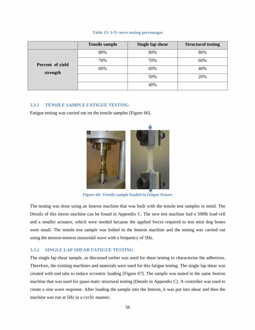
56

Table 13: S-N curve testing percentages

Tensile sample Single lap shear Structural testing

Percent of yield

strength

80% 80% 80%

70% 70% 60%

60% 60% 40%

50% 20%

40%

3.3.1 TENSILE SAMPLE FATIGUE TESTING

Fatigue testing was carried out on the tensile samples [Figure 66].

Figure 66: Tensile sample loaded in fatigue fixture

The testing was done using an Instron machine that was built with the tensile test samples in mind. The

Details of this intron machine can be found in Appendix C. The new test machine had a 500lb load cell

and a smaller actuator, which were needed because the applied forces required to test mini dog bones

were small. The tensile test sample was bolted in the Instron machine and the testing was carried out

using the tension-tension sinusoidal wave with a frequency of 5Hz.

3.3.2 SINGLE LAP SHEAR FATIGUE TESTING

The single lap shear sample, as discussed earlier was used for shear testing to characterize the adhesives.

Therefore, the existing machines and materials were used for this fatigue testing. The single lap shear was

created with end tabs to reduce eccentric loading [Figure 67]. The sample was tested in the same Instron

machine that was used for quasi-static structural testing (Details in Appendix C). A controller was used to

create a sine wave response. After loading the sample into the Instron, it was put into shear and then the

machine was run at 5Hz in a cyclic manner.

57

Figure 67: Single lap shear - side view [50]

3.3.3 STRUCTURAL SAMPLE FATIGUE TESTING

The last fatigue test that was carried out was on the structural T-sample. The same Instron machine and

LCF that were used to test the structural samples were also used for the fatigue testing. In addition, the

sinusoidal wave, producing shear loading in the sample, was used with a frequency of 5Hz, which is the

same as all the fatigue testing that was undertaken previously.

Adhesive End tab

58

Chapter 4 : RESULTS AND DISCUSSIONS

4.1 : COMPARISON OF NUMERICAL AND EXPERIMENTAL RESULTS

The initial goal of this thesis was to carry out a structural test that would then be used to verify the

accuracy of the numerical material models that were created. Therefore, comparing the numerical

simulation data with the experimental test data helped to evaluate the accuracy of the adhesive material

models. All the experimental tests and numerical simulations results were reported in terms of load (kN)

and displacement (mm).

SA9850 was structurally tested with two surface preparations: grit blasting and a contaminated surface. It

was found that the contaminated surface resulted in better data because it was more consistent. Therefore,

the experimental test data obtained from the contaminated surface preparation was used for this study.

The details of all the tests and the comparison of the grit blasting and contaminated surface can be found

in Appendix I.

4.1.1 QUASI-STATIC TESTING

The first step was to analyze the numerical simulation results for DP460NS. The force-displacement for

the quasi-static structural testing simulation was found [Figure 68]. The displacement comprised of the

failure of the adhesive as well as plastic deformation of the adherend. It was found that there were two

distinct parts of the graph [Figure 68]:

Section 1 – ramp up

Section 2 – Adherend Plastic deformation and adhesive deformation

The ramp up stage, as discussed in the boundary condition section, was because the impact plate that

interacts with the sample was misaligned by 1.5 degrees at the start of the test. Once the sample was

aligned with the impact plate the deformation of the adherend and the adhesive began.

59

Figure 68: DP460NS quasi-static shear numerical simulation force-displacement result

At the end of the test, the adhesive failed and the adherend underwent plastic deformation [Figure 69].

Much of this plastic deformation occurred in the horizontal C-channel.

Figure 69: Quasi static cohesive simulation – DP460NS – deformation before failure

Section 1 Section 2

60

A comparison between the numerical simulation and the experimental test showed the plastic deformation

that occurred in the horizontal aluminum C-channel [Figure 70]. The opening distance was also assessed

and it was found that the numerical simulation captured the deformation of the horizontal C-channel for

both DP460NS and SA9850 [Table 14].

Figure 70: Deformation of horizontal section during quasi-static shear testing - Numerical simulation (left)

and experimental test (right)

Table 14: Quasi-static shear experimental and numerical horizontal C-channel deformation comparison

Average opening

(mm)

DP460NS SA9850

Experimental Test 42.0 44.6

Numerical Simulation 45.0 45.2

Difference (%) 6.90 1.34

Figure 71 illustrates the experimental data vs. the numerical simulation for shear of DP460NS in quasi-

static testing. The average maximum force, displacement to failure and energy were calculated and the

numerical simulation and experimental tests were compared [Table 15]. The difference for all these

parameters was found to be approximately 10% but all these numerical values fell within the 95%

confidence interval (CI) obtained for the experimental tests [Figure 72]. In addition, analysis software

(CORA) was used to evaluate the shape of the graphs, which is represented by the cross correlation value

[Table 16]. For this test, it was found that the cross correlation value resulted in an excellent rating, which

shows that the numerical simulation graph shape was similar to the experimental tests. Taking all these

Opening

61

parameters into consideration it was concluded that the numerical simulation accurately captured the

behavior of the DP460NS quasi-static shear tests.

Figure 71: DP460NS quasi-static shear numerical simulation vs. experimental tests

Table 15: DP460NS quasi-static shear numerical simulation vs. experimental tests displacement, force and

energy comparison

Average Maximum

Displacement (mm)

Average Maximum

Force (kN)

Energy

(kN-mm)

Experimental Test

(95% confidence

interval)

3.00 (±0.56) 30.48 (±3.9) 40.59

(±12.81)

Numerical Simulation 3.28 26.84 46.56

Difference (%) 8.92 12.70 13.7

62

Figure 72: DP460NS Quasi-static shear - Experimental test 95% CI for displacement, force and Energy

compared to numerical simulation

Table 16 DP460NS Quasi-static shear – Cross correlation and size

Cross Correlation

Function Size

DP460NS 1 0.995 0.987

DP460NS 2 0.968 0.893

DP460NS 3 0.988 0.945

Average 0.984 0.942

Rating Excellent Excellent

Figure 74 shows the SA9850 data for the numerical simulation vs. the experimental tests with the

contaminated surface preparation. The SA9850 numerical simulation captures the experimental tests well

except for the third experimental test. This sample exhibited a larger displacement when compared to the

two other tests. Upon investigating the samples after failure, it was found that the spew fillet on the third

sample was not cleaned. The addition of a spew fillet has been shown in multiple studies to increase the

63

failure strength of epoxy adhesives. [81, 82] This larger amount of energy absorption observed by the

third SA9850 sample can therefore be attributed to the spew fillet [Figure 73].

Figure 73: Spew fillet

Therefore, when the third data set was excluded, the maximum force and energy are approximately 4%

different when comparing the numerical simulations and the experimental tests [Table 17]. The numerical

simulation over predicted the displacement at failure by 15% and did not fall within the 95% confidence

interval of the experimental tests [Figure 75]. The last two values that were used to evaluate the accuracy

of this numerical model were the cross correlation (Excellent) and the size (Good) ratings [Table 18],

both of which show that the numerical simulation results were in agreement with the experimental tests.

Similar to DP460NS, the conclusion for SA9850 is that the numerical simulation was able to simulate the

behavior of the adhesive for the quasi-static shear experimental test.

Figure 74: SA9850 quasi-static shear numerical simulation vs. experimental tests

64

Table 17: SA9850 quasi-static shear numerical simulation vs. experimental testsdisplacement, force and

energy comparison

Average Maximum

Displacement (mm)

Average Maximum

Force (kN)

Energy

(kN-mm)

Experimental Test

(95% confidence

interval)

2.92 (±0.15) 28.02 (±0.84) 45.77

(±21.55)

Numerical Simulation 3.36 26.88 47.92

Difference (%) 14.01 4.15 4.59

Figure 75: SA9850 Quasi-static shear - Experimental test 95% CI for displacement, force and Energy

compared to numerical simulation

65

Table 18: SA9850 Quasi-static shear – Cross correlation and size

Cross Correlation

Function Size

SA9850 1 0.983 0.757

SA9850 2 0.998 0.915

Average 0.991 0.836

Rating Excellent Good

4.1.2 TORSIONAL TESTING

For both adhesives in torsion, the cohesive elements began to fail at the same corner in the numerical

simulation [Figure 76, marked as one]. As the cohesive elements failed, they eroded in the same direction

[Figure 76]. This gradual failure was seen after the maximum force was reached [Figure 77, Figure 79].

Figure 76: Quasi-static torsion simulation - start

The simulation for DP460NS in torsion captured the initial stage when compared to the experimental tests

but failed at a lower displacement and force [Figure 77]. This difference can also be seen when the

experimental test and numerical simulation maximum force, energy [Table 19], cross correlation value

and the size value [Table 20] were compared. All these comparisons show that the numerical simulation

does not capture the experimental tests. Lastly, the failure seemed to be gradual in the simulation as the

elements erode, which was unlike the test because it failed instantly. From these results it was important

to consider the fact that during torsion the primary mode of loading is a Mode III form of loading, which

is an out of plane shear [34]. This model of loading was not tested previously and therefore this lack of

1

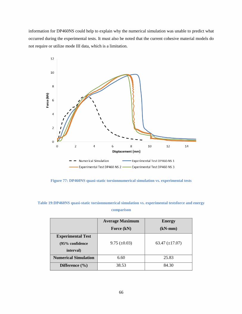
66

information for DP460NS could help to explain why the numerical simulation was unable to predict what

occurred during the experimental tests. It must also be noted that the current cohesive material models do

not require or utilize mode III data, which is a limitation.

Figure 77: DP460NS quasi-static torsionnumerical simulation vs. experimental tests

Table 19:DP460NS quasi-static torsionnumerical simulation vs. experimental testsforce and energy

comparison

Average Maximum

Force (kN)

Energy

(kN-mm)

Experimental Test

(95% confidence

interval)

9.75 (±0.03) 63.47 (±17.07)

Numerical Simulation 6.60 25.83

Difference (%) 38.53 84.30

67

Figure 78: DP460NS Quasi-static torsion - Experimental test 95% CI for force and Energy compared to

numerical simulation

Table 20: DP460NS Quasi-static torsion – Cross correlation and size

Cross Correlation

Function Size

DP460NS 1 0.643 0.265

DP460NS 2 0.664 0.307

DP460NS 3 0.617 0.304

Average 0.641 0.292

Rating Fair Marginal

Unlike the DP460NS torsional results, the SA9850 numerical simulation predicted the behavior of the

adhesive [Figure 79]. The energy was over predicted by the numerical simulation by 24.6% but fell within

the 95% confidence interval [Figure 80]. The maximum force (2.9% difference) and the shape of the

force-displacement curve, which resulted in a cross correlation rating of excellent [Table 21] showed that

the numerical simulation matched well with the experimental tests.

68

Although the numerical simulation for SA9850 in torsion is capable of capturing the behavior of the

experimental tests, it is still important to keep in mind that no previous testing was carried on the mode III

loading for SA9850.

Figure 79: SA9850 quasi-static torsionnumerical simulation vs. experimental tests

Table 21 : SA9850quasi-static torsionnumerical simulation vs. experimental testsforce and energy

comparison

Average Maximum

Force (kN)

Energy

(kN-mm)

Experimental Test

(95% confidence

interval)

6.84 (±1.17) 23.21 (±10.72)

Numerical Simulation 7.05 29.79

Difference (%) 2.90 24.53

69

Figure 80: SA9850 Quasi-static torsion - Experimental test 95% CI for force and Energy compared to

numerical simulation

Table 22: SA9850 Quasi-static torsion – Cross correlation and size

Cross Correlation

Function Size

SA9850 1 0.953 0.722

SA9850 2 0.787 0.594

SA9850 3 0.987 0.881

Average 0.909 0.732

Rating Excellent Good

4.1.3 DYNAMIC IMPACT

The numerical simulation results for DP460NS and SA9850 showed that the adhesive did not fail. The

aluminum C-channels deformed and absorbed all the energy while the adhesive held the two C-channels

together [Figure 81], which is the same result as that found experimentally. An evaluation was carried out

to ensure that the deformations in the numerical simulation were consistent with the deformations that

were observed in the experiment.

70

Figure 81: Unsupported dynamic impact simulation before the test (left) and after the test (right)

The maximum deformation of the horizontal C-channel was evaluated at two points as indicated by the

red dots [Figure 82].

Figure 82: Unsupported dynamic impact numerical simulation (left) vs. experimental test (right)

It was found that the difference for the deformation of the horizontal C-channel between the numerical

simulation and the experimental test at these points was 2% and 5.4% for DP460NS and SA9850

respectively [Table 23].

71

Table 23: Unsupported dynamic impact experimental and numerical horizontal C-channel deformation

comparison

Average Displacement (mm)

DP460NS SA9850

Experimental Test 5.1 6.5

Numerical Simulation 5.2 6.2

Difference (%) 2.0 5.4

At the maximum force when the velocity of the impact goes to 0 m/s, the aluminum underwent elastic

unloading, hence the displacement reversal seen at the end of the graph [Figure 83].

For the DP460NS unsupported dynamic impact, the numerical simulation and experimental tests were

compared [Figure 83]. The percent difference between the numerical simulation and the experimental test

for displacement (2.5%) and energy (5%) were both good [Table 24]. These positive results were also

validated by the cross correlation rating of excellent [Table 25].

Figure 83: DP460NS Unsupported dynamic impact numerical simulation vs. experimental tests

72

Table 24: DP460NS Unsupported dynamic impact numerical simulation vs. experimental tests displacement

and energy comparison

Average Maximum

Displacement (mm)

Energy

(kN-mm)

Experimental Test

(95% confidence interval) 7.4 (±0.64) 156 (±2.64)

Numerical Simulation 7.59 164

Difference (%) 2.5 5.0

Figure 84: DP460NS unsupported dynamic impact - Experimental test 95% CI for force and Energy

compared to numerical simulation

73

Table 25: DP460NS unsupported dynamic impact - Cross correlation and size

Cross Correlation

Function Size

DP460NS 1 0.971 0.853

DP460NS 2 0.96 0.79

DP460NS 3 0.964 0.792

DP460NS 4 0.968 0.727

DP460NS 5 0.971 0.853

Average 0.967 0.803

Rating Excellent Good

When comparing the SA9850 experimental tests to the numerical simulations [Figure 85] it was found

that the initial peak was not captured, which is the case with all the dynamic impact experiments. Similar

to the analysis results for DP460NS, the difference between the displacement, energy [Figure 85], CI

comparison [Figure 86] and cross correlation values [Table 27] all show that this numerical simulation

accurately captured what occurred in the experimental tests.

Figure 85: SA9850 Unsupported dynamic impact numerical simulation vs. experimental tests

74

Table 26: SA9850 Unsupported dynamic impact numerical simulation vs. experimental test displacement and

energy comparison

Average Maximum

Displacement (mm)

Energy

(kN-mm)

Experimental Test

(95% confidence

interval)

7.94 (±0.7) 155 (±2.75)

Numerical Simulation 8.35 176

Difference (%) 5.0 12.7

Figure 86: SA9850 unsupported dynamic impact - Experimental test 95% CI for force and Energy compared

to numerical simulation

75

Table 27: SA9850 unsupported dynamic impact - Cross correlation and size

Cross Correlation

Function Size

SA9850 1 0.978 0.964

SA9850 2 0.975 0.860

SA9850 3 0.967 0.875

Average 0.973 0.900

Rating Excellent Excellent

The unsupported dynamic impact for DP460NS showed a good comparison between the numerical

simulation and the experimental tests [Figure 87]. With a support, the deformation of the adherend was

reduced significantly and the energy was absorbed through the failure of the adhesive.

Figure 87: DP460NS dynamic impact with a supportnumerical simulation vs. experimental tests

During the impact, the numerical simulation showed that a small amount of deformation was observed in

the horizontal C-channel but most of the force and the deformation was the adhesive as it sheared and

failed [Figure 88].

76

Figure 88: Supported dynamic impact simulation before the test (left) and after the test (right)

The numerical simulation and the experimental tests for DP460NS showed a difference of 3.7% when

comparing their energy absorption [Table 28]. As for the maximum force and the displacement, both are

under predicted in the numerical model by 22.3% and 24.3% respectively. Although these differences are

high, the maximum force result from the numerical simulation is found to be within the 95% CI for the

experimental test [Figure 89]. In addition, the cross correlation function rating was found to be excellent

[Table 29]. Therefore, the numerical simulation captures the experimental tests well when all the

comparison parameters are considered.

Table 28: DP460NS supported dynamic impact numerical simulation vs. experimental tests displacement,

force and energy comparison

Average Maximum

Displacement (mm)

Average Maximum

Force (kN)

Energy

(kN-mm)

Experimental Test

(95% confidence

interval)

3.64 (±0.32) 58.9 (±15.0) 79.2 (±22.1)

Numerical Simulation 2.85 47.1 82.1

Difference (%) 24.3 22.3 3.6

77

Figure 89: DP460NS supported dynamic impact - Experimental test 95% CI for force and Energy compared

to numerical simulation

Table 29: DP460NS supported dynamic impact - Cross correlation and size

Cross Correlation

Function Size

DP460NS 1 0.937 0.7

DP460NS 2 0.923 0.786

Average 0.93 0.743

Rating Excellent Good

Lastly, the SA9850 numerical simulation results were compared to the supported dynamic impact tests

[Figure 90].The numerical simulation showed similar results to DP460NS. Comparing the average

maximum force and displacement it was found that the numerical simulation under predicted by

approximately 20% for both [Table 30]. The difference for energy was found to be 5.7%. The force result

from the numerical simulation was found to fall within the 95% CI for the experimental test [Figure 91].

Lastly, the cross correlation function and the size both resulted in a rating of excellent [Table 31].

78

Therefore, taking all the comparison parameters into consideration it can be concluded that the numerical

simulation captures the experimental tests.

Figure 90: SA9850 supported dynamic impact numerical simulation vs. experimental tests

Table 30: SA9850 supported dynamic impact tnumerical simulation vs. experimental tests displacement,

force and energy comparison

Average Maximum

Displacement (mm)

Average Maximum

Force (kN)

Energy

(kN-mm)

Experimental Test

(95% confidence

interval)

3.71 (±) 57.38 (±) 86.21 (±)

Numerical Simulation 3.0 45.5 81.3

Difference (%) 19.2 21.4 5.7

79

Figure 91: SA9850 supported dynamic impact - Experimental test 95% CI for force and Energy compared to

numerical simulation

Table 31: SA9850 supported dynamic impact - Cross correlation and size

Cross Correlation

Function Size

SA9850 1 0.879 0.707

SA9850 2 0.946 0.982

SA9850 3 0.933 0.95

Average 0.919 0.88

Rating Excellent Excellent

80

4.1 FATIGUE TESTING RESULTS

4.1.1 DOG BONE FATIGUE RESULTS

The fatigue data for DP460NS and SA9850 in a dog bone configuration were obtained. Using the data, an

S-N curve was plotted for both adhesives [Figure 92]. The thick black line found on the edge of the

figure represented the limit at which the fatigue life was assumed to be infinite. The adhesive was

assumed to be at “infinite” life at 10^7 cycles (approximately 23 days testing at a frequency of 5Hz) [83].

This was only an assumption and tests still needed to be carried out to ensure that it holds true for these

structural adhesives. The reason this was not completed was due to difficulties that were encountered with

the equipment when attempting to run the fatigue testing for a prolonged amount of time.

Figure 92: Dog bone fatigue data S-N curve for DP460NS and SA9850

4.1.2 SINGLE LAP SHEAR FATIGUE RESULTS

The fatigue data for DP460NS and SA9850 [Figure 93] in a single lap shear configuration were both

obtained.

81

Figure 93: DP460NS and SA9850 percentage of maximum force vs. cycle’s to failure - Single lap shear fatigue

As one can see for both adhesives, the cycles to failure do not decrease linearly as the stress amplitude

was reduced. This was due to the fact that during the test there was bending that was observed in the

aluminum. The adherend bending [Figure 94] created a stress concentration at the edges [Figure 95].

These stress concentrations at the edges, which resulted in a non-uniform shear distribution, caused the

adherend to fail at 50%. With these failures and the bending affects, the test was unable to produce fatigue

data for the adhesive at the lower percentages. This non-linear S-N curve emphasizes the effects and

importance of joint design. If a joint design is done incorrectly, it can lead to weaker fatigue qualities.

Figure 94: Single lap shear bending during test

82

Figure 95: Stress distribution in the adhesive in a single lap shear example [40]

Although changing the adherend was considered, it was ultimately decided that regardless of the adherend

choice, there was always going to be an inherent problem with this test due to the non-uniform stress

distribution along the bond line.

4.1.3 STRUCTURAL SAMPLE FATIGUE RESULTS

The structural fatigue testing was carried out at four stress percentages and only for DP460NS [Figure

96]. The single lap shear fatigue and the structural fatigue data were compared because they were both

joints with a mixed mode loading but predominantly shear stresses. The structural testing followed a

similar pattern to the single lap shear [Figure 96]. The single lap shear and the structural testing both

resulted in a non-linear S-N curve. This shows the extent by which the mixed mode loading affected the

fatigue life of the adhesive. It also further emphasized the importance of joint design to maximize the

strength as well as the fatigue life of a structure.

83

Figure 96: Fatigue S-N curve for DP460NS single lap shear vs structural testing

84

Chapter 5 : SUMMARY AND RECOMMENDATIONS

5.1 SUMMARY

Structural test samples were created by adhesively joining two aluminum C-channels. The structural

samples were tested using two toughened structural epoxy adhesives (DP460NS and SA9850) in four

configurations:

Quasi-static direct shear (2.5mm/min)

Quasi-static torsion (2.5mm/min)

Unsupported dynamic impact in direct shear (25 kg impacting at 4.43 m/s)

Supported dynamic impact in direct shear (25 kg impacting at 3.96 m/s)

In general, the four experimental tests demonstrated consistent responses concerning shape, maximum

force and displacement at failure. In addition, it was found that the dynamic impact forces at failure were

larger than the quasi-static forces at failure. This result was expected because both adhesives were strain

rate dependent.

Corresponding finite element models were developed for each test, using cohesive elements to model the

adhesive joint and incorporating material properties from tests on bulk adhesive (tensile tests) and

coupon-level tests (lap shear). The C-channels were modeled with solid elements, determined to be

necessary to model the impact and deformation of the adherends. Imaging from the experiments was used

to identify some challenges with the first model iteration. Importantly, the test was sensitive to the

boundary conditions including the test sample alignment, and the compliance of the test fixture. A

boundary condition sensitivity study was undertaken to identify the importance of the sample position and

alignment, and a detailed model of the test fixture was created to incorporate the fixture compliance in the

model. Finally, a mesh convergence study was undertaken and identified a mesh size of 2 mm as

appropriate for this model in quasi-static and dynamic loading.

The numerical models of the direct shear tests were in very good agreement with the experiments. The

cross-correlation rating for the quasi-static tests was 0.984 for DP460NS and 0.991 for SA9850, which

are both considered to be excellent. In torsion, the numerical simulation was in good agreement for the

SA9850, but for the DP460NS the numerical simulation predicted a lower force and displacement

compared to the experimental tests. It is therefore important to carry out testing in Mode III for DP460NS

to gain a better understanding of what the energy release rate in mode III is for this adhesive. It is also

important to test SA9850 in mode III and compared the results to DP460NS. With these tests, a better

85

understanding can be obtained of why the numerical simulation for SA9850 in torsion was more accurate.

For dynamic impact, both numerical models were in good agreement with the experimental results. This

was demonstrated using cross-correlation factor to compare the shape of the curves, which resulted in

excellent ratings.

It was discovered that for all the numerical simulations the predicted force was below the average force

measured in the experimental tests. This was due to the fact that the constitutive material models were

created based on work done with the thick adherend lap shear test. These thick adherend lap shear tests

produced relatively good shear data but were not in pure shear. To address this limitation, improved test

data should be measured using pure shear loading, such as in the pin and collar test. Another issue with

the thick adherend lap shear test data is that the surface preparation that was carried out for all the tests

was simply cleaning the surface. It has been proven that surface preparation can have an effect on the

strength of the adhesive joint. Therefore, it is recommended that this testing be undertaken again with grit

blasted surface preparation for DP460NS and a contaminated surface preparation for SA9850.

Fatigue testing was undertaken for three different test sample configurations. Tension-tension testing on

bulk adhesive material in a tensile sample configuration resulted in a log-linear relationship between the

applied stress amplitude and number of cycles to failure. It must be noted that an added benefit to using

the tensile test sample for fatigue is that the adhesive is visible. This would allow for future tests where

damage can potentially be observed during fatigue testing. When testing single lap shear samples, which

incorporate mixed mode loading and a stress concentration factor, the result was a non-linear relationship

between the applied stress amplitude and the number of cycles. This testing revealed that at lower stress

amplitudes the effects of the bending of the adherend caused early failure of the joint and in many cases

resulted in failure of the adherend and not the adhesive, emphasizing the importance of joint design.

Structural fatigue testing was carried out to observe the fatigue behavior of the adhesive in a larger

configuration. It was found that the response was generally similar in shape to the single lap shear sample,

but with reduced number of load cycles for a given stress amplitude. This difference can be attributed to

the larger adhesion area in the structural sample when compared to the single lap shear sample, and

therefore a higher likelihood of defects in the joint that could initiate fatigue failure. The fatigue testing

undertaken in this thesis represents a first attempt at measuring relevant material performance at the bulk,

coupon and structural levels.

86

The primary goal of this research was to demonstrate the ability to model adhesive joints in structures

subject to static and dynamic loading, to enable the incorporation of adhesives into vehicles through CAE

and to support the integration and design of multi-material lightweight structures.

5.2 RECOMMENDATIONS

The main recommendation for DP460NS and SA9850 is to improve the shear material data.

Carry out a Mode III test on both adhesives to gain a better understanding of the torsional

behavior of the adhesive and to compare the energy release rates in Mode III.

For SA9850, it was shown that the surface preparation in the structural tests showed high

variability. It is recommended that these coupon-level tests be repeated using the Dry Lube

surface preparation to be consistent with the data from the testing in this work.

87

APPENDIX A: STRUCTURAL SAMPLE SPECIFICATIONS AND

MANUFACTURING

MECHANICAL DRAWINGS

The C-channels used in the structural testing are aluminum 6063-T5.

88

89

90

91

MANUFACTURING PROCES FOR STRUCTURAL TEST SAMPLES

1. Cut and machine C-channels to the correct sizes. The ends of the C-channels were milled to

ensure accurate and consistent sizes.

2. Create all the holes using a template. This involved creating 4 holes on the horizontal channel and

for the torsion sample one hole in the horizontal channel

Figure 97: Horizontal channel with four holes (left), Vertical channel with one hole (left)

3. There were two forms of surface preparation that were carried out, Grit blasting and dry lube to

contaminate the surface

-For grit blasting the C-channels were placed in a grit-blasting machine and sand was

used. Grit blasting was done to ensure the surface roughness is equal for all channels.

After grit blasting, MEK (Methyl Ethyl Ketone) was used to clean surface from

contaminants.

-The other form of surface preparation was simply placing dry lube E1 on the surface for

SA9850 to mimic a contaminated surface

4. Use fixture to join the two C-channels into a T-shape configuration.

-Apply adhesive and place brass shims to ensure the thickness of the adhesive is

consistent.

92

Figure 98: Fixture for creating the structural test samples

5. Once the adhesive and the C-channels were clamped down in the fixture, it was placed into an

oven to cure the adhesive.

6. After removing the samples from the oven, the excess adhesive was removed to ensure that the

adhesive had a consistent area and that no spew fillet was left.

93

APPENDIX B: FATIGUE SAMPLE SPECIFICATIONS

Tensile test size

Single lap shear

94

APPENDIX C: TEST MACHINE DETAILS

5.1 Quasi-static shear, torsion and fatigue single lap shear test rig

This machine was a custom quasi-static hydraulic machine:

A 407 controller (MTS Systems Corporation) was used to control the hydraulic distribution and therefore

the custom quasi-static hydraulic machine.

Load cell

Company: Transducer Techniques

Model: SWP-20k

Capacity: 20,000lb

Hydraulic Cylinder

Company: Parker

Model: KJJ2HPS23A/23A

95

5.2 Tensile test sample fatigue test rig

The tensile test rig is also a custom rig. It was designed to test mini dogbones, which are sensitive to large

forces and required very little force to fail or fatigue.

Load cell

Company: Omega

Model: LC412-500

Capacity: 500lb

Hydraulic Cylinder

Company: MTS Systems Corporation

Model: 204.11

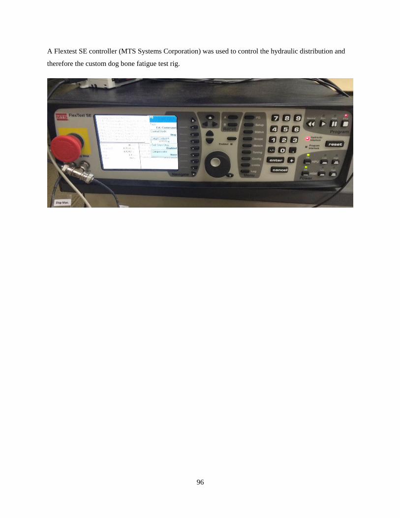
96

A Flextest SE controller (MTS Systems Corporation) was used to control the hydraulic distribution and

therefore the custom dog bone fatigue test rig.

97

5.3 Dynamic impact test rig

The dynamic impact test rig was a Rosand Precision IFW5 drop tower tester.

Mass that is used for the impact. It

is lifted and dropped at the

predetermined height.

Piezoelectric Load cell

Company: Kistler Technologies

Model: 9071A

Capacity: 400kN

98

APPENDIX D: FIXTURE EVOLUTION

An initial experiment was carried out with the first fixture that was created, also known as the high

compliance fixture (HCF) [Figure 99]. The data that was collected from this initial test was as expected

from the material and coupon level tests that were carried out previously. That is to say, that the forces

that were experienced during this initial structural test were similar the single lap shear testing. After

reviewing the initial data and camera footage, it was found that due to the fixture design and the

deformation of the test samples a large amount of elastic deformation was observed in the test fixture.

This meant that the deformation that was recorded by the LVDT was larger than the deformation that the

testing sample underwent. In the initial HCF, the sample was bolted to each column individually. This

setup caused a large moment to occur, which in turn caused the fixture to elastically deform. This created

a problem because for the numerical simulations only the test sample would be simulated and not the

entire fixture. This meant that even though some error can always be attributed to compliance in the

machine and fixture, any compliance issues would not be captured in the simulation. The HCF was

modified and strengthened to decrease the amount of elastic deformation in the fixture that was found in

the initial tests. This new low compliance fixture (LCF) would lead to less compliance in the machine and

therefore help to ensure that the simulations could be kept simple while still being accurate.

Figure 99: High compliance quasi-static fixture - HCF

The new LCF incorporated a solid steel bar that was welded to both columns. Onto this bar, a piece of

steel was welded and reinforced [Figure 100]. The sample then sat over the steel section and was quasi-

statically tested using an upward moving flat plate. This simple change in the fixture reduced the elastic

99

deformation and compliance of the machine. This helped to insure that the complexity of the simulation

and the cost with regards to time would not be increased by having to simulate the fixture as well.

Figure 100: Low compliance Quasi-static shear fixture - LCF

Similar to the quasi-static test, more than one fixture was created to complete the dynamic impact testing.

The first fixture was a simple fixture with two columns [Figure 101]. The sample was bolted into each

column and the mass was dropped. This was preliminary testing and was used to gain a better

understanding of the experimental test. This fixture was then strengthened and new supports were added

to reduce the vibration and compliance that was observed.

Figure 101: Dynamic impact initial fixture unsupported

100

APPENDIX E: TESTING FIXTURES

Quasi-static Design 1– HCF

101

Quasi-static Design 2– LCF- Main fixture

102

Quasi-static Torsion

103

Drop tower fixture

104

APPENDIX F: MESH CONVERGENCE ANALYSIS

The mesh convergence study was carried out on the high deformation test with a simple support. The test

was carried out with the following element sizes: 0.2mm, 1mm, 2mm and 4mm.

Figure 102: Mesh refinement from left to right (4mm, 2mm, 1mm, 0.2mm)

The following graphs show the results for displacement, energy absorbed and time to completion for all

the mesh sizes. It can be seen that at 2mm the displacement and energy absorbed have converged. The

time required to completion increases exponentially and with all this information 2mm was used as the

mesh size for the simulations.

105

106

APPENDIX G: LS-DYNA CARDS

Test Material Model Implicit or Explicit

Quasi-static Shear MATERIAL NUMBER

186 and MATERIAL

NUMBER 240 without

strain rate

Implicit/Explicit

Quasi-static Torsion MATERIAL NUMBER

186 and MATERIAL

NUMBER 240 without

strain rate

Implicit/Explicit

Supported dynamic

impact

MATERIAL NUMBER

240 with strain rate

Explicit

Unsupported dynamic

impact

MATERIAL NUMBER

240 with strain rate

Explicit

DP460NS MATERIAL NUMBER 186 Quasi-static

$ COHESIVE ELEMENTS

$

$ THIS MATERIAL NEEDS TO BE DEFINE USING A SINGLE LAYER OF SOLID ELEMENTS

$ THEREFORE IT REQUIRES THE DEFINITION OF A *PART CARD

$ AND A *SECTION_SOLID CARD

$ THE ORIENTATION OF THE ELEMENT MUST BE PROPER, SEE LS-DYNA MANUAL

*PART

adhesive

2,2,2

$

$

*SECTION_SOLID

2,20

$

*MAT_COHESIVE_GENERAL

$

107

$

$MID, RO, ROFLG, INTFAIL TES, TSLC, GIC, GIIC

2, 1.20E-9, 0, 1, 0, 1000, 2.82061, 15.733205

$

$XMU, T, S, STFSF

1, 37.57, 20.67, 0

$

$

*DEFINE_CURVE

$ LCID, SIDR, SFA corrected scale of displacement

1000, ,2.2

$

0.00,0.00

0.03,0.73

0.05,0.87

0.07,0.93

0.09,0.97

0.11,0.98

0.22,1.00

0.35,1.00

0.47,0.98

0.55,0.96

0.58,0.92

0.61,0.85

0.64,0.73

0.66,0.62

1.00,0.00

$

DP460NS MATERIAL NUMBER 240 Quasi-static

$

108

$ MAT # 240

*MAT_COHESIVE_MIXED_MODE_ELASTOPLASTIC_RATE

$

$ INCLUDES STRAIN RATE EFFECTS. ELEMENT SIZES LESS THAN 1mm IN THICKNESS

SHOULD BE USE WITH THIS MODEL

$

$ MATERIAL PROPERTIES DP-460NS USING EXPERIMENTAL DATA INCLUDING STRAIN

RATE EFFECTS

$

$MID, RO, ROFLG, INTFAIL, EMOD, GMOD, THICK, OUTPUT

2, 1.20E-9, 0, 0, 2.18E3, 0.77E3, 0, XXXX

$ OUTPUT= XXX, USE SAME AS D3PLOT FRQ

$ THICK =0 SO IT USES THE ACTUAL ELEMENT COORDINATES FOR THICKNESS TO

CALCULATE STIFFNESS

$

$

$UNITS FOR GC ENTRY ARE MPa x mm WHICH IS CONSISTENT WITH ENERGY RELEASE

RATE

$G1C_0, G1C_INF, EDOT_G1, TO, T1, EDOT_T, FG1

$-2.5, 7.6 , 0.4896, -31.95, -3.5, 0.0001263, 0.75 (8-12-2014)

-2.82, 4.15, 0.54, -31.95, -3.5, 0.0001263, 0.35

$G2C_0, G2C_INF, EDOT_G2, SO, S1, EDOT_S, FG2

$-10.48, 6.3, 0.0041, -23.89, -1.0153, 0.005, 0.77 (8-12-2014)

15.0, 0, 0, -23.890000, -1.0153, 0.005, 0.770000

$

$

SA9850 MATERIAL NUMBER 186 Quasi-static

$$$$$$$$$$$$$$$$$$$$$$$$$$$$$$$$$$$$$$$$$$$$$$$$$$$$$$$$$$

$

$ COHESIVE ELEMENTS

$

$

$$$$$$$$$$$$$$$$$$$$$$$$$$$$$$$$$$$$$$$$$$$$$$$$$$$$$$$$$$

$

109

$

$ THIS MATERIAL NEEDS TO BE DEFINE USING A SINGLE LAYER OF SOLID ELEMENTS

$ THEREFORE IT REQUIRES THE DEFINITION OF A *PART CARD

$ AND A *SECTION_SOLID CARD

$ THE ORIENTATION OF THE ELEMENT MUST BE PROPER, SEE LS-DYNA MANUAL

$

*PART

adhesive

2,2,2

$

*SECTION_SOLID

2,20

$

*MAT_COHESIVE_GENERAL

$

$ GIC & GIIC FIT TO TENSILE & LAP SHEAR

$ T FROM TENSILE TEST, S FROM SHEAR TEST

$

$ID, RO, ROFLG, INTFAIL TES, TSLC, GIC, GIIC

$2, 1.20e-9, 0, 1, 0, 1000, 7.68, 5.3

$UPDATE 04/11/2014

$2, 1.20e-9, 0, 1, 0, 1000, 2.974, 1.487

$ UPDATE NOV-26-104

2, 1.20e-9, 0, 1, 0, 1001, 2.974, 15

$UNITS FOR GIC ENTRY ARE MPa x mm WHICH IS CONSISTENT WITH ENERGY RELEASE

RATE

$

$XMU, T, S, STFSF

$1, 30.55, 20.84, 0

$ UPDATE 04/11/2014

1, 28.19, 24.9, 0

*DEFINE_CURVE

1000

0, 0

110

0.05, 0.8

0.1, 0.95

0.125, 0.965

0.15, 0.975

0.2, 0.98

0.5, 1

0.65, 0.96

0.75, 0.9

0.8, 0.65

1, 0

$

* DEFINE_CURVE

1001

0.000, 0.000

0.022, 0.296

0.072, 0.699

0.095, 0.739

0.116, 0.749

0.136, 0.754

0.157, 0.759

0.177, 0.765

0.198, 0.773

0.219, 0.781

0.239, 0.789

0.260, 0.798

0.281, 0.806

0.301, 0.814

0.322, 0.821

0.343, 0.829

0.363, 0.836

0.384, 0.844

0.404, 0.852

0.425, 0.860

0.446, 0.868

111

0.467, 0.877

0.487, 0.886

0.508, 0.895

0.529, 0.905

0.550, 0.914

0.570, 0.923

0.591, 0.931

0.612, 0.940

0.632, 0.948

0.653, 0.956

0.674, 0.963

0.694, 0.971

0.715, 0.978

0.735, 0.986

0.756, 0.993

0.777, 1.000

1.000, 0.000

$

$

$

SA9850 MATERIAL NUMBER 240 Quasi-static

$ MAT # 240 WITH STRAIN RATE EFFECTS

$

$WITH STRAIN RATE EFFECTS

$

*MAT_COHESIVE_MIXED_MODE_ELASTOPLASTIC_RATE

$

$

$ MATERIAL PROPERTIES SA-9850 USING EXPERIMENTAL DATA FROM SNPE-2000 AS

PRESENTED ABOVE FOR MATERIAL #240

$

$

$MID, RO, ROFLG, INTFAIL, EMOD, GMOD, THICK, OUTPUT

2, 1.20E-9, 0, 0, 2.4E3, 0.85E3, 0, XXXX

112

$ OUTPUT= XXX, USE SAME AS D3PLOT FRQ

$ THICK =0 SO IT USES THE ACTUAL ELEMENT COORDINATES FOR THICKNESS TO

CALCULATE STIFFNESS

$

$

$UNITS FOR GC ENTRY ARE MPa x mm WHICH IS CONSISTENT WITH ENERGY RELEASE

RATE

$G1C_0, G1C_INF, EDOT_G1, TO, T1, EDOT_T, FG1

-4.39, 24.86, 0.0103, -23.90, -2.86, 0.000186, 0.3

$G2C_0, G2C_INF, EDOT_G2, SO, S1, EDOT_S, FG2

$ 8.92, 0, 0, 24.9, 0, 0, 0.78 (*use this line if strain rate effects in shear want to be voided*)

-3.757, 3.705, 3.94, -17, -0.328, 4.41e-13, 0.78

$

$

$

Aluminum Material Mode:

*MAT_POWER_LAW_PLASTICITY_TITLE

Aluminum

$# mid ro e pr k n srcsrp

4 2.7100E-9 64000.000 0.300000 301.39999 0.123000

$# sigyvpepsf

142.000 0.000 0.000

113

APPENDIX H: NUMERICAL SIMULATION EVOLUTION

The numerical simulation results found throughout the thesis are the final outcomes. To reach these

results multiple iterations of the numerical simulations and boundary condition refinements were

undertaken. This appendix shows the numerical simulations that were undertaken and the changes that

were done to more accurately capture what occurred in the experimental tests.

QUASI STATIC SHEAR

With a straight wall the simulation did not exhibit the initial shallow ramp up that was observed in the

experimental tests. To remedy this problem the impacting wall in the simulation was angled similar to

what was observed in the experimental tests. Another problem with the original simulation is that the

block that the horizontal C-channel sits over was simulated as a solid rigid block. This was found to give

good results but the displacement that was simulated fell short of what was found through the testing.

Therefore, the boundary condition for the block was modified to capture the elastic deformation that

occurred in the steel bar during the testing. The block was extended and the edges of the block were

constrained. This allowed the center section, which housed the horizontal C-channel to deform elastically

as was observed during the testing

Therefore, a combination of a lack of an angled impact wall and a solid block in the initial numerical

simulations resulted in an incorrect displacement prediction.

Old Simulation

114

New Simulation

115

SUPPORTED DYNAMIC IMPACT TEST

No compliance

The following graphs show the numerical simulation without the compliance section that was added at the

bottom. The main difference was that the initial ramp up in the numerical simulation is stiffer than that

found in the experimental tests. This was observed for both DP460NS and SA9850.

Old simulation New simulation

Force Measurement 1

Force Measurement 2

116

Another problem that was observed was the position at which the force was found in the numerical

simulation. In the experimental test, the load cell is located below the fixture. In the numerical simulation,

the force data can be obtained from two points, at the wall impact and at the bottom. This was compared

in the following graphs and it was shown that taking the measurement from the bottom creates a smoother

ramp up but also captures all the noise that occurs as the maximum force is reached. When the

measurement is taken from the top, the force-displacement result is smooth.

117

UNSUPPORTED DYNAMIC IMPACT TEST

Without a fixture, the numerical simulation showed a very steep ramp up as the adhesive failed. In

addition, instead of the maximum force occurring at a singular point it occurs over a 2mm displacement,

which did not capture the experimental tests. To more accurately capture the boundary conditions the

simulation was redone with the fixture and this addition changed the force-displacement curve.

118

Old simulation New Simulation

119

APPENDIX I: EXPERIMENTAL RESULTS COMPARING HCF AND LCF

AND SURFACE PREPERATION

DP460NS QUASI-STATIC DIRECT SHEAR EXPERIMENTAL RESULTS

The force-displacement results were found from the HCF set up at a quasi-static rate for DP460NS

[Figure 103]. The deformation found below is not just that of the adhesive but of the entire sample, in

which some plastic deformation of the Aluminum was observed during the experimental test

It must also be noted that although this is called a quasi-static shear test, the sample was observed to

undergo a more complex mixed mode loading. This occurred because as the sample was pushed, the

adherend began to plastically deform, which caused the adhesive to go from a shear to a mixed mode-

loading scenario.

The data from this initial test showed variability. Looking at the graphs it can be seen that the ramp up

section is different for most of the tests. This variation makes it difficult to use this set of data to verify

the numerical simulations. It is also an undesirable set of data as much of the displacement that is

observed is it that of the fixture, which was not simulated because simulating the effects of the entire

fixture and the sample, would be computationally expensive.

Figure 103: Quasi-static– DP460NS - Shear - HCF

120

The quasi-static test was redone with the new LCF. This test was again carried out on the same hydraulic

tester with a modified fixture to reduce the elastic deformation. This data, unlike that found in the initial

test, shows a better data set [Figure 104]. The ramp up and displacement is similar and consistent.

Figure 104: Quasi-static – DP460NS - Shear - LCF

After reviewing the videos of the testing it was found that during the initial contact between the sample

and the moving plate, there was a slight misalignment of 1.5 degrees. This misalignment caused an initial

shallow ramp up that is highlighted in red [Figure 104]. This observation was important as it would affect

the boundary condition that would be used in the simulation.

Although looking at the graphs showed an improvement and better consistency with the LCF, it was

important to carry out a simple statistical analysis to verify the improvement [Table 32]. The main aspect

that was of importance was the displacement at failure. It was found that the standard deviation was

approximately two times smaller when comparing the HCF to the LCF. This decrease in the standard

deviation in displacement helps to show that the inconsistencies that were found in the HCF were down to

the large amount of deformation that the fixture underwent.

121

Table 32: Statistical analysis of DP460NS – HCF vs. NCF

Average Max Min Standard Deviation

HCF - Force 19.2 24 15 3.53

HCF - Displacement 4.0 4.9 3.4 0.6

LCF - Force 30.5 31.7 28.6 1.6

LCF - Displacement 3.0 3.3 2.8 0.23

SA9850 QUASI-STATIC DIRECT SHEAR EXPERIMENTAL RESULTS

The force-displacement curves were also obtained for SA9850 on the HCF [Figure 105]. Similar to the

results found for DP460NS, it was found that by switching to the LCF [Figure 106] more consistent data

was observed with a contaminated surface preparation. This was also verified when comparing the

standard deviation of the displacements of the HCF and the LCF with a contaminated surface [Table 33].

Figure 105: Quasi-static – SA9850 - Shear - HCF

122

Table 33: Statistical analysis of SA9850 with a contaminated surface – HCF vs. LCF

Average Max Min Standard Deviation

HCF - Force 14.9 17.2 12.5 2

HCF - Displacement 3.2 4 2.7 0.6

LCF– Force (Contaminated surface)* 28.02 28.2 27.9 0.2

LCF– Displacement (Contaminated surface)* 2.92 2.95 2.9 0.03

*This Data does not include sample 3 due to spew fillet

Figure 106: Quasi-static – SA9850 - Shear – LCF – Grit blasted

The main concern that was observed with the SA9850 on the LCF was the variation in the data with a grit

blasted surface preparation [Figure 106]. Although the data looks relatively consistent with regards to the

ramp up, two samples failed prematurely. Upon investigating the failures, it was seen that the two

samples that failed earlier failed in an interfacial manner [Figure 107]. The difference in strength can also

be seen in the amount of deformation that the horizontal adherend section underwent. The horizontal

adherend with the cohesive failure plastically deformed more than the horizontal section with the

123

interfacial failure [Figure 108]. This again emphasizes the importance of surface preparation to obtain the

best results for adhesives.

Figure 107: Surface failure of SA9850 grit blasted - Interfacial failure (right) and cohesive failure (Left)

Figure 108: SA9850 grit blasted - Horizontal section deformation comparison - Interfacial failure (right) and

cohesive failure (Left)

In comparison to the grit blasted surface preparation the contaminated surface showed good consistency,

which can be seen when comparing the standard deviations of displacement and force [Table 34]. This is

because SA9850 was designed to be optimized when used with a contaminant on the surface. Test sample

3 shows a failure that occurred at a higher displacement than the first two tests [Figure 110]. Upon

investigating the samples after failure, it was found that the spew fillet on the third sample was not

cleaned. The addition of a spew fillet has been shown in multiple papers to increase the failure strength of

epoxy adhesives. [81, 82] This larger amount of energy absorption observed by the third SA9850 sample

can therefore be attributed to the spew fillet [Figure 109].

124

Figure 109: Spew fillet

Table 34: SA9850 LCF grit blasted vs. contaminated surface experimental test results

Surface Preparation Attribute Average Max Min Standard

Deviation

Grit blasted

Force 25.2 30.6 19.6 4.67

Displacement 2.5 4 1.2 1.47

Contaminated

surface*

Force 28.02 28.2 27.9 0.19

Displacement 2.92 2.95 2.9 0.03

*This Data does not include sample 3 due to spew fillet

125

Figure 110: Quasi-static SA9850 with a contaminated surface in Shear – LCF

DP460NS TORSION EXPERIMENTAL RESULTS

The following figure shows the torsional results for the DP460NS [Figure 111]. As one can see, the data

is relatively consistent for the ramp up, as well as the force and the displacement [Table 35].

After analyzing the video using tracker software, no problems (such as bolt slipping) or compliance issues

were observed.

Table 35: Statistical analysis of DP460NS

Average Max Min Standard Deviation

Maximum Force 9.8 9.8 9.6 0.01

Displacement at maximum

force

7.8 8.5 7.4 0.45

126

Figure 111: Quasi-static DP460NS torsion test results

SA9850 TORSION EXPERIMENTAL RESULTS

The SA9850 also showed good consistency for both the grit blasted tests [Figure 112] and the

contaminated surface preparation [Figure 113]. The contaminated surface preparation had a higher force

and underwent a larger deformation before failing when compared to the grit blasted preparation [Table

36]. These results are expected from surface preparation testing that was previously carried out.

Table 36: Statistical analysis of SA9850 grit blasted and contaminated surface

Average Max Min Standard Deviation

Grit blasted - Maximum Force 3.9 4.2 3.4 0.45

Contaminated - Maximum Force 6.8 8.1 6.2 0.8

Grit blasted - Displacement at

maximum force

2.1 2.3 2.0 0.15

Contaminated - Displacement at

maximum force

4.0 4.6 3.5 0.46

127

Figure 112: Quasi-static SA9850 with grit blast - torsion test results

Figure 113: Quasi-static SA9850 with contaminated surface- torsion test results

DP460NS DYNAMIC IMPACT EXPERIMENTAL RESULTS

The force-displacement for the DP460NS unsupported dynamic impact tests were collected [Figure 114].

The data was consistent with regards to the displacements and the maximum forces. In this test, there was

no failure of the adhesive. The entire deformation that occurred was the adherend plastically deforming.

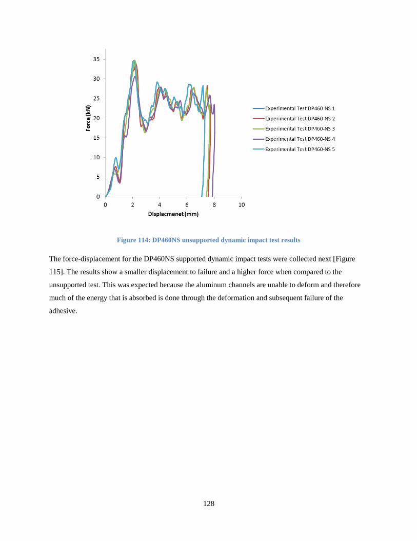
128

Figure 114: DP460NS unsupported dynamic impact test results

The force-displacement for the DP460NS supported dynamic impact tests were collected next [Figure

115]. The results show a smaller displacement to failure and a higher force when compared to the

unsupported test. This was expected because the aluminum channels are unable to deform and therefore

much of the energy that is absorbed is done through the deformation and subsequent failure of the

adhesive.

129

Figure 115: DP460NS supported dynamic impact test results

SA9850 DYNAMIC IMPACT EXPERIMENTAL RESULTS

The following results are for the SA9850 adhesive in the dynamic impact tests. Four separate tests were

carried out on the SA9850:

Test 1: boundary condition – Unsupported, Surface finish – Grit blasted [Figure 116]

Test 2: boundary condition – Unsupported, Surface finish – Contaminated Surface [Figure 117]

Test 3: boundary condition – Supported, Surface finish – Grit [Figure 118]

Test 4: boundary condition – Supported, Surface finish - Contaminated Surface [Figure 119]

Test 1, which tested the SA9850 with a grit blasted surface finish, showed a similar result to that observed

at a quasi-static rate [Figure 116]. The failure of the adhesive occurred at different displacements and

unlike DP460NS, even without a support all of the samples showed adhesive failure except for one

sample. This inconsistency can be attributed to the grit blasting surface finish because with a

contaminated surface this adhesive failure was not observed.

130

Figure 116: SA9850 grit blasted unsupporteddynamic impact test results

The testing carried out on the SA9850 with a contaminated surface resulted in a more consistent set of

data [Figure 117]. This showed that the ideal surface preparation for SA9850 was a contaminated surface

such as the dry lube E1 that was used in this thesis. With this contaminated surface, the SA9850 did not

fail because the adherend deformed and absorbed all the energy, which was a similar result to the

DP460NS.

Figure 117: SA9850 contaminated surface unsupported dynamic impact test results

131

With a support boundary condition, the same results concerning surface preparation were observed for

SA9850. The contaminated surface preparation [Figure 119] resulted in an increase of 20% energy

absorption at failure when compared to the grit blasted [Figure 118].

Figure 118: SA9850 grit blasted unsupported dynamic impact test results

Figure 119:SA9850 contaminated surface unsupported dynamic impact test results

132

SA9850 SURFACE PREPARATION CONCLUSION

For SA9850 the contaminated surface and the grit blasted surface preparation experimental test results

were compared:

Quasi-static shear showed that the contaminated surface resulted in lower standard deviations for

displacement and force.

Quasi-static torsion showed the force and displacement were double for the contaminated surface

preparation.

The unsupported dynamic impact test resulted in no adhesive failure with a contaminated surface

preparation.

For the supported dynamic impact, the energy absorption was 20% more for the contaminated

surface vs. the grit blasted surface preparation.

From looking at all the SA9850 experimental data in the quasi-static and dynamic impact tests it was

concluded that the contaminated surface data would be used to compare to the numerical simulations.

This was due to the fact that the contaminated surface resulted in more consistent and higher strength data

when compared to the grit blasted surface preparation.

133

APPENDIX J: STRAIN RATE AFFECTS ON THE NUMERICAL

SIMULATION

The SA9850 dynamic impact numerical models were tested without strain rate dependence.

The unsupported numerical simulation that did not include strain rate for the SA9850 predicted that the

adhesive fails [Figure 120]. Although there was a large amount of deformation in the adherends, in the

end the cohesive elements failed and eroded. This cohesive failure predicted by the numerical simulation

without strain rate affects for SA9850 is undesirable because none of the experimental tests showed

adhesive failure for SA9850. As for the numerical simulation with a strain rate, it was found that the

cohesive elements did not fail and the simulation was in better agreement with the experimental tests.

Figure 120: SA9850 unsupported dynamic impact numerical simulation vs. experimental tests

The same result was found for the supported dynamic impact simulation for SA9850. Without the strain

rate affects the numerical simulation underpredicted the displacement to failure and the energy required to

fail the adhesives [Figure 121].

134

Figure 121: SA9850 supported dynamic impact numerical simulation vs. experimental tests

135

REFERENCES

[1] Soren Anderson, Ian Parry, James M. Sallee, and Carolyn Fischer, "Automobile Fuel Economy Standards:

Impacts, Efficiency, and Alternatives," 2010.

[2] Obama Administration Finalizes Historic 54.5 mpg Fuel Efficiency Standards/ Consumer Savings Comparable

to Lowering Price of Gasoline by $1 Per Gallon by 2025. Available:

http://yosemite.epa.gov/opa/admpress.nsf/bd4379a92ceceeac8525735900400c27/13f44fb4e2c2d39d85257a68005d0

154!OpenDocument

[3] Monthly monitoring of vehicle fuel economy and emissions. Available:

http://www.umich.edu/~umtriswt/EDI_sales-weighted-CAFE.html

[4] G. Fontaras and Z. Samaras, "On the way to 130 g CO2/km—Estimating the future characteristics of the average

European passenger car," Energy Policy, vol. 38, pp. 1826-1833, 4, 2010.

[5] C. De Fur, A. Richardson, A. Roach and G. Wiesent, "US and german regulations of CO2 emissions from

passenger cars," in Globalization and Public PolicyAnonymous Springer, 2015, pp. 137-155.

[6] Anonymous "New Car CO2 Report 2015, The 14th report,".

[7] Y. Orbach and G. E. Fruchter, "Forecasting sales and product evolution: The case of the hybrid/electric car,"

Technological Forecasting and Social Change, vol. 78, pp. 1210-1226, 9, 2011.

[8] J. Wiedemann, The Influence of Ground Simulation and Wheel Rotation on Aerodynamic Drag Optimization-

Potential for Reducing Fuel Consumption, 1996.

[9] Lamborghini Aventador LP700 body and rolling shell revealed. [Online]. Available:

http://www.caradvice.com.au/106327/lamborghini-aventador-lp700-body-and-rolling-shell-revealed/

[10] W. S. Miller, L. Zhuang, J. Bottema, A. J. Wittebrood, P. De Smet, A. Haszler and A. Vieregge, "Recent

development in aluminium alloys for the automotive industry," Materials Science and Engineering: A, vol. 280, pp.

37-49, 3/15, 2000.

[11] The official U.S government source for fuel economy information. Available: http://www.fueleconomy.gov/

[12] S. Birch, "Audi, Lamborghini cross borders with multimaterial R&amp;D and production," 2011.

[13] A. Kinloch, "Toughening epoxy adhesives to meet today's challenges," MRS Bull, vol. 28, pp. 445-448, 2003.

136

[14] T. A. Barnes and I. R. Pashby, "Joining techniques for aluminium spaceframes used in automobiles: Part II —

adhesive bonding and mechanical fasteners," J. Mater. Process. Technol., vol. 99, pp. 72-79, 3/1, 2000.

[15] P. Peddiraju, A. Papadopoulous and R. Singh, "CAE framework for aerodynamic design development of

automotive vehicles," in 3rd ANSA & μETA International Conference, 2009, .

[16] Anonymous "History of adhesives," Tech. Rep. Volume 1, Issue 2, 1991.

[17] G. Rowland, "Adhesives and adhesion," CHEM NZ, vol. 71, pp. 17, 1998.

[18] 3M’s Structural Two‐Part Epoxy Adhesive Performance vs. Mechanical Fasteners. [Online]. Available:

http://multimedia.3m.com/mws/mediawebserver?mwsId=SSSSSufSevTsZxtUO8tBPY_ZevUqevTSevTSevTSeSSS

SSS--

[19] A. J. Kinloch, S. J. Shaw and D. L. Hunston, "Deformation and fracture behaviour of a rubber-toughened

epoxy: 2. Failure criteria," Polymer, vol. 24, pp. 1355-1363, 10, 1983.

[20] A. J. Kinloch, S. J. Shaw, D. A. Tod and D. L. Hunston, "Deformation and fracture behaviour of a rubber-

toughened epoxy: 1. Microstructure and fracture studies," Polymer, vol. 24, pp. 1341-1354, 10, 1983.

[21] A. Kin Loch and S. Shaw, "The fracture resistance of a toughened epoxy adhesive," The Journal of Adhesion,

vol. 12, pp. 59-77, 1981.

[22] A. F. Yee and R. A. Pearson, "Toughening mechanisms in elastomer-modified epoxies," J. Mater. Sci., vol. 21,

pp. 2462-2474, 1986.

[23] 3 Scotch-Weld TM Epoxy Adhesives DP460 Off-White DP460 NS - Technical Data. [Online]. Available:

http://multimedia.3m.com/mws/media/66122O/3mtm-scotch-weld-tm-epoxy-adhesive-dp460-ns-and-off-white.pdf

[24] L. F. M. da Silva, R. D. Adams and M. Gibbs, "Manufacture of adhesive joints and bulk specimens with high-

temperature adhesives," Int J Adhes Adhes, vol. 24, pp. 69-83, 2, 2004.

[25] L. Trimiño, Private Communication, 2015.

[26] Impact Resistant Structural Adhesive SA9850. Available: http://multimedia.3m.com/mws/media/880082O/3m-

impact-resistant-structural-adhesive-sa9850.pdf

[27] M. J. Davis and A. McGregor, "Assessing adhesive bond failures: Mixed-mode bond failures explained," in

ISASI Australian Safety Seminar, Canberra, 2010, pp. 4-6.

137

[28] A. Rudawska, "Selected aspects of the effect of mechanical treatment on surface roughness and adhesive joint

strength of steel sheets," Int J Adhes Adhes, vol. 50, pp. 235-243, 2014.

[29] J. S. Tomblin, Fatigue and Stress Relaxation of Adhesives in Bonded Joints. Office of Aviation Research,

Federal Aviation Administration, 2003.

[30] R. F. Wegman and J. Van Twisk, Surface Preparation Techniques for Adhesive Bonding. William Andrew,

2012.

[31] Y. Nandwani, Private Communication, 2015.

[32] B. Broughton and M. Gower, "Preparation and testing of adhesive joints," 2001.

[33] Adhesive Failure & Epoxy Failure. Available: http://theadhesivesexpert.com/adhesives-failure-epoxy-failure/

[34] A. B. de Morais, A. B. Pereira, M. F. S. F. de Moura and A. G. Magalhães, "Mode III interlaminar fracture of

carbon/epoxy laminates using the edge crack torsion (ECT) test," Composites Sci. Technol., vol. 69, pp. 670-676, 4,

2009.

[35] S. L. Donaldson, "Mode III interlaminar fracture characterization of composite materials," Composites Sci.

Technol., vol. 32, pp. 225-249, 1988.

[36] Z. Chen, R. Adams and L. F. da Silva, "Fracture toughness of bulk adhesives in mode I and mode III and curing

effect," Int. J. Fract., vol. 167, pp. 221-234, 2011.

[37] E. E. Medeiros, da Silva Dias, Avelino Manuel and A. L. Christoforo, "Numerical Simulation of Mechanical

Fracture Testings," International Journal of Materials Engineering, vol. 2, pp. 61-66, 2012.

[38] K. DeVries and P. Borgmeier, "Testing of adhesives," Handbook of Adhesive Technology, Marcell Dekker,

New York, pp. 223-253, 2003.

[39] ASTM D3165 - 07(2014), "Standard practice for preparing, cleaning, and evaluating corrosion test specimens,"

2014.

[40] G. Kelly, "Joining of carbon fibre reinforced plastics for automotive applications," 2004.

[41] S. Park and M. Seo, Interface Science and Composites. Academic Press, 2011.

[42] J. A. Nairn, "Energy release rate analysis for adhesive and laminate double cantilever beam specimens

emphasizing the effect of residual stresses," Int J Adhes Adhes, vol. 20, pp. 59-70, 2, 2000.

138

[43] R. Smerd, S. Winkler, C. Salisbury, M. Worswick, D. Lloyd and M. Finn, "High strain rate tensile testing of

automotive aluminum alloy sheet," Int. J. Impact Eng., vol. 32, pp. 541-560, 2005.

[44] A. Standard, "Standard test method for tensile properties of plastics," ASTM International.Designation: D, vol.

638, 2003.

[45] C. Thunert, "CORA Release 3.6 User’s Manual," GNS mbH, Germany, 2012.

[46] D. Cesari, S. Compigne, R. Scherer, L. Xu, N. Takahashi, M. Page, K. Asakawa, G. Kostyniuk, E. Hautmann,

K. Bortenschlager, M. Sakurai and T. Harigae, "WorldSID Prototype Dummy Biomechanical Responses," Stapp

Car Crash J., vol. 45, pp. 285-318, Nov, 2001.

[47] Clarke M., Buckley M., Broughton J.G., Hutchinson A.R., "Characterisation and simulation of structural

adhesives," 7th European LS_DYNA COnference, 2009.

[48] N. -. Hoang, A. -. Hanssen, M. Langseth and R. Porcaro, "Structural behaviour of aluminium self-piercing

riveted joints: An experimental and numerical investigation," Int. J. Solids Structures, vol. 49, pp. 3211-3223, 11/15,

2012.

[49] A. M. Girão Coelho and F. S. K. Bijlaard, "Experimental behaviour of high strength steel end-plate

connections," Journal of Constructional Steel Research, vol. 63, pp. 1228-1240, 9, 2007.

[50] S. W. Jones, P. A. Kirby and D. A. Nethercort, "The analysis of frames with semi-rigid connections — A state-

of-the-art report," Journal of Constructional Steel Research, vol. 3, pp. 2-13, 1983.

[51] F. Seeger, M. Feucht, G. Dumitru and T. Graf, "Enhancement of Spot Weld modeling using MAT_100_DAI. 7

th LS-DYNA Forum," Bamberg, Germany, 2008.

[52] J. A. Swanson, D. S. Kokan and R. T. Leon, "Advanced finite element modeling of bolted T-stub connection

components," Journal of Constructional Steel Research, vol. 58, pp. 1015-1031, 2002.

[53] F. Vivio, "A new theoretical approach for structural modelling of riveted and spot welded multi-spot

structures," Int. J. Solids Structures, vol. 46, pp. 4006-4024, 11, 2009.

[54] Anonymous "Chapter 14: Fatigue," ASM International. Elements of Metallurgy and Engineering Alloys, 2008.

[55] Introduction to Finite Element Analysis (FEA) or Finite Element Method (FEM). Available:

http://www.engr.uvic.ca/~mech410/lectures/FEA_Theory.pdf

[56] I. B. Barna Szabo, Finite Element Analysis. 1991.

139

[57] A. Javidinejad, "FEA Practical Illustration of Mesh-Quality-Results Differences between Structured Mesh and

Unstructured Mesh," International Scholarly Research Notices, vol. 2012, 2012.

[58] Hourglass. Available: http://www.dynasupport.com/howtos/element/hourglass

[59] S. Bala and J. Day, "General guidelines for crash analysis in LS-DYNA,".

[60] B. Moran, M. Ortiz and C. Shih, "Formulation of implicit finite element methods for multiplicative finite

deformation plasticity," Int J Numer Methods Eng, vol. 29, pp. 483-514, 1990.

[61] T. Bui, "Explicit and Implicit Methods In Solving Differential Equations," 2009.

[62] Z. Kazancı and K. Bathe, "Crushing and crashing of tubes with implicit time integration," Int. J. Impact Eng.,

vol. 42, pp. 80-88, 4, 2012.

[63] F. Dogan, H. Hadavinia, T. Donchev and P. S. Bhonge, "Delamination of impacted composite structures by

cohesive zone interface elements and tiebreak contact," Central European Journal of Engineering, vol. 2, pp. 612-

626, 2012.

[64] A. T. Zachariah, "Finite Element Modelling of Adhesive Interface between Steel and CFRP," 2006.

[65] L. Rincon, "Analysis and Performance of Adhesively Bonded Crush Tube Structures," 2012.

[66] Anonymous "LS-DYNA® KEYWORD USER'S MANUAL<br /> VOLUME II Material Models " 2012.

[67] S. Marzi, L. Ramon-Villalonga, M. Poklitar, F. Kleiner, I. Fraunhofer, A. Henkel and C. KGaA, "Usage of

cohesive elements in crash analysis of large, bonded vehicle structures experimental tests and simulation," in

German LS-Dyna Forum Bamberg, Pages BI, 2008, .

[68] D. M. Parks, "The virtual crack extension method for nonlinear material behavior," Comput. Methods Appl.

Mech. Eng., vol. 12, pp. 353-364, 12, 1977.

[69] J. R. Rice, "A path independent integral and the approximate analysis of strain concentration by notches and

cracks," Journal of Applied Mechanics, vol. 35, pp. 379-386, 1968.

[70] D. Xie and S. B. Biggers Jr., "Progressive crack growth analysis using interface element based on the virtual

crack closure technique," Finite Elements Anal. Des., vol. 42, pp. 977-984, 7, 2006.

[71] D. M. Parks, "A stiffness derivative finite element technique for determination of crack tip stress intensity

factors," Int. J. Fract., vol. 10, pp. 487-502, 1974.

140

[72] L. G. Margolin, "A generalized Griffith criterion for crack propagation," Eng. Fract. Mech., vol. 19, pp. 539-

543, 1984.

[73] K. Gordnian, H. Hadavinia, P. J. Mason and E. Madenci, "Determination of fracture energy and tensile

cohesive strength in Mode I delamination of angle-ply laminated composites," Composite Structures, vol. 82, pp.

577-586, 2, 2008.

[74] K. Park and G. H. Paulino, "Cohesive zone models: a critical review of traction-separation relationships across

fracture surfaces," Appl. Mech. Rev., vol. 64, pp. 060802, 2011.

[75] P. Reed and S. Spearing, "Research project: An evaluation of cohesive zone models for adhesive failure in

bonded joints," .

[76] S. Marzi, O. Hesebeck, M. Brede and F. Kleiner, "A rate-dependent, elasto-plastic cohesive zone mixed-mode

model for crash analysis of adhesively bonded joints," in 7th European LS-DYNA Conference, 2009, .

[77] R. D. S. G. Campilho, M. D. Banea, J. A. B. P. Neto and L. F. M. da Silva, "Modelling adhesive joints with

cohesive zone models: effect of the cohesive law shape of the adhesive layer," Int J Adhes Adhes, vol. 44, pp. 48-56,

7, 2013.

[78] I. Barsoum, F. Khan, A. Molki and A. Seibi, "Modeling of ductile crack propagation in expanded thin-walled

6063-T5 aluminum tubes," Int. J. Mech. Sci., vol. 80, pp. 160-168, 3, 2014.

[79] J. A. Harris and P. A. Fay, "Fatigue life evaluation of structural adhesives for automative applications," Int J

Adhes Adhes, vol. 12, pp. 9-18, 1, 1992.

[80] G. G. Tantina, "Design with plastics," ASM Hanbook, vol. 20, pp. 639, 1997.

[81] M. Tsai and J. Morton, "The effect of a spew fillet on adhesive stress distributions in laminated composite

single-lap joints," Composite Structures, vol. 32, pp. 123-131, 1995.

[82] M. You, Z. Yan, X. Zheng, H. Yu and Z. Li, "A numerical and experimental study of adhesively bonded

aluminium single lap joints with an inner chamfer on the adherends," Int J Adhes Adhes, vol. 28, pp. 71-76, 2008.

[83] W. Broughton, R. Mera and G. Hinopoulos, "Cyclic Fatigue Testing of Adhesive Joints: Test Method

Assessment," NPL Report CMMT (A), vol. 191, pp. 1996-1999, 1999.