experimental study on turbulent boundary-layer ows with ...1154071/fulltext01.pdfexperimental study...
TRANSCRIPT

Experimental study on turbulentboundary-layer flows with wall transpiration
by
Marco Ferro
October 2017
Technical Reports
Royal Institute of Technology
Department of Mechanics
SE-100 44 Stockholm, Sweden

Akademisk avhandling som med tillstand av Kungliga Tekniska Hogskolan iStockholm framlagges till offentlig granskning for avlaggande av teknologiedoktorsexamen fredag den 24 November 2017 kl 10:15 i Kollegiesalen, KungligaTekniska Hogskolan, Brinellvagen 8, Stockholm.
TRITA-MEK 2017:13ISSN 0348-467XISRN KTH/MEK/TR-17/13-SEISBN 978-91-7729-556-3
c©Marco Ferro 2017
Universitetsservice US–AB, Stockholm 2017
Experimental study on turbulent boundary-layer flows withwall transpiration
Marco Ferro
Linne FLOW Centre, KTH Mechanics, Royal Institute of TechnologySE-100 44 Stockholm, Sweden
AbstractWall transpiration, in the form of wall-normal suction or blowing through apermeable wall, is a relatively simple and effective technique to control the be-haviour of a boundary layer. For its potential applications for laminar-turbulenttransition and separation delay (suction) or for turbulent drag reduction andthermal protection (blowing), wall transpiration has over the past decades beenthe topic of a significant amount of studies. However, as far as the turbulentregime is concerned, fundamental understanding of the phenomena occurringin the boundary layer in presence of wall transpiration is limited and consid-erable disagreements persist even on the description of basic quantities, suchas the mean streamwise velocity, for the rather simplified case of flat-plateboundary-layer flows without pressure gradients.
In order to provide new experimental data on suction and blowing boundarylayers, an experimental apparatus was designed and brought into operation. Theperforated region spans the whole 1.2 m of the test-section width and with itsstreamwise extent of 6.5 m is significantly longer than previous studies, allowingfor a better investigation of the spatial development of the boundary layer. Thequality of the experimental setup and measurement procedures was verifiedwith extensive testing, including benchmarking against previous results on acanonical zero-pressure-gradient turbulent boundary layer (ZPG TBL) and ona laminar asymptotic suction boundary layer.
The present experimental results on ZPG turbulent suction boundarylayers show that it is possible to experimentally realize a turbulent asymptoticsuction boundary layer (TASBL) where the boundary layer mean-velocityprofile becomes independent of the streamwise location, so that the suction rateconstitutes the only control parameter. TASBLs show a mean-velocity profilewith a large logarithmic region and without the existence of a clear wake region.If outer scaling is adopted, using the free-stream velocity and the boundarylayer thickness (δ99) as characteristic velocity and length scale respectively,the logarithmic region is described by a slope Ao = 0.064 and an interceptBo = 0.994, independently from the suction rate (Γ). Relaminarization of aninitially turbulent boundary layer is observed for Γ > 3.70× 10⁻³. Wall suctionis responsible for a strong damping of the velocity fluctuations, with a decreaseof the near-wall peak of the velocity-variance profile ranging from 50% to 65%when compared to a canonical ZPG TBL at comparable Reτ . This decrease inthe turbulent activity appears to be explained by an increased stability of thenear-wall streaks.
iii

Measurements on ZPG blowing boundary layers were conducted for blowingrates ranging between 0.1% and 0.37% of the free-stream velocity and coverthe range of momentum thickness Reynolds number 10 000 / Reθ / 36 000.Wall-normal blowing strongly modifies the shape of the boundary-layer mean-velocity profile. As the blowing rate is increased, the clear logarithmic regioncharacterizing the canonical ZPG TBLs gradually disappears. A good overlapamong the mean velocity-defect profiles of the canonical ZPG TBLs and of theblowing boundary layers for all the Re number and blowing rates considered isobtained when normalization with the Zagarola-Smits velocity scale is adopted.Wall blowing enhances the intensity of the velocity fluctuations, especially inthe outer region. At sufficiently high blowing rates and Reynolds number, theouter peak in the streamwise-velocity fluctuations surpasses in magnitude thenear-wall peak, which eventually disappears.
Key words: Turbulent boundary layer, boundary-layer suction, boundary-layerblowing, wall-bounded turbulent flows, self-sustained turbulence.
iv

Experimentell studie av turbulenta gransskikt medvaggenomstromning
Marco Ferro
Linne FLOW Centre, KTH Mekanik, Kungliga Tekniska HogskolanSE-100 44 Stockholm, Sverige
SammanfattningGenom att anvanda sig av genomstrommande ytor, med sugning eller blasning,kan man relativt enkelt och effektivt paverka ett gransskikts tillstand. Genom sinpotential att paverka olika stromningsfysikaliska fenomen sa som att senarelaggabade avlosning och omslaget fran laminar till turbulent stromning (genomsugning) eller som att exempelvis minska luftmotstandet i turbulenta gransskiktoch ge kyleffekt (genom blasning), sa har ett otaligt antal studier genomforts paomradet de senaste decennierna. Trots detta sa ar den grundlaggande forstaelsenbristfallig for de stromningsfenomen som intraffar i turbulenta gransskikt overgenomstrommande ytor. Det rader stora meningsskiljaktigheter om de mestelementara stromningskvantiteterna, sasom medelhastigheten, nar sugning ochblasning tillampas aven i det mest forenklade gransskiktsfallet namligen detsom utvecklar sig over en plan platta utan tryckgradient.
For att ta fram nya experimentella data pa gransskikt med sugning ochblasning genom ytan sa har vi designat en ny experimentell uppstallning samttagit den i bruk. Den genomstrommande ytan spanner over hela breddenav vindtunnelns matstracka (1.2 m) och ar 6.5 m lang i stromningsriktningenoch ar darmed betydligt langre an vad som anvants i tidigare studier. Dettagor det mojligt att battre utforska gransskiktet som utvecklas over ytan istromningsriktningen. Kvaliteten pa den experimentella uppstallningen och valdamatprocedurerna har verifierats genom omfattande tester, som aven inkluderarbenchmarking mot tidigare resultat pa turbulenta gransskikt utan tryckgradienteller blasning/sugning och pa laminara asymptotiska sugningsgransskikt.
De experimentella resultaten pa turbulenta gransskikt med sugning bekraftarfor forsta gangen att det ar mojligt att experimentellt satta upp ett turbulentasymptotiskt sugningsgransskikt dar gransskiktets medelhastighetsprofil bliroberoende av stromningsriktningen och dar sugningshastigheten utgor den endakontrollparametern. Det turbulenta asymptotiska sugningsgransskiktet visar sigha en medelhastighetsprofil normalt mot ytan med en lang logaritmisk regionoch utan forekomsten av en yttre vakregion. Om man anvander yttre skalningav medelhastigheten, med fristromshastigheten och gransskiktstjockleken somkaraktaristisk hastighet respektive langdskala, sa kan det logaritmiska omradetbeskrivas med en lutning pa Ao = 0.064 och ett korsande varde med y-axeln paBo = 0.994, som ar oberoende av sugningshastigheten. Om sugningshasighetennormaliserad med fristromshastigheten overskrider vardet 3.70×10⁻³ sa atergardet ursprungligen turbulenta gransskiktet till att vara laminart. Sugningengenom vaggen dampar hastighetsfluktuationerna i gransskiktet med upp till
v

50− 60% vid direkt jamforelse av det inre toppvardet i ett turbulent gransskiktutan sugning och vid jamforbart Reynolds tal. Denna minskning av turbulentaktivitet verkar harstamma fran en okad stabilitet av hastighetsstraken narmastytan.
Matningar pa turbulenta gransskikt med blasning har genomforts forblasningshastigheter mellan 0.1 och 0.37% av fristromshastigheten och tackerReynoldstalomradet (10−36)×103, med Reynolds tal baserat pa rorelsemangds-tjockleken. Vid blasning genom ytan far man en stark modifiering av formen pahastighetesfordelningen genom gransskiktet. Nar blasningshastigheten okar sakommer till slut den logaritmiska regionen av medelhastigheten, karaktaristiskfor turbulent gransskikt utan blasning, att gradvis forsvinna. God overens-stammelse av medelhastighetsprofiler mellan turbulenta gransskikt med ochutan blasning erhalls for alla Reynoldstal och blasningshastigheter nar profil-erna normaliseras med Zagarola-Smits hastighetsskala. Blasning vid vaggenokar intensiteten av hastighetsfluktuationerna, speciellt i den yttre regionen avgransskiktet. Vid riktigt hoga blasningshastigheter och Reynoldstal sa kommerden yttre toppen av hastighetsfluktuationer i gransskiktet att overskrida deninre toppen, som i sig gradvis forsvinner.
Nyckelord: Turbulent gransskikt, gransskiktssugning, gransskiktsblasning,vaggbundna turbulenta floden, sjalv-forsorjande turbulens.
vi

Other publications
The following paper, although related, is not included in this thesis.
Marco Ferro, Robert S. Downs III & Jens H. M. Fransson, 2015.Stagnation line adjustment in flat-plate experiments via test-section venting.AIAA Journal 53 (4), pp. 1112–1116.
Conferences
Part of the work in this thesis has been presented at the following internationalconferences. The presenting author is underlined.
Marco Ferro, Robert S. Downs III, Bengt E. G. Fallenius & JensH. M. Fransson. On the development of turbulent boundary layer with wallsuction. 68th Annual Meeting of the APS Division of Fluid Mechanics. Boston,2015.
Marco Ferro, Bengt E. G. Fallenius & Jens H. M. Fransson. On theturbulent boundary layer with wall suction. 7th iTi Conference in Turbulence.Bertinoro, 2016. DOI: 10.1007/978-3-319-57934-4 6.
Marco Ferro, Bengt E. G. Fallenius & Jens H. M. Fransson. Onthe scaling of turbulent asymptotic suction boundary layers. 10th internationalsymposium on Turbulence and Shear Flow Phenomena (TSFP10). Chicago,2017.
vii


Contents
Abstract iii
Sammanfattning v
Introduction 1
Chapter 1. Basic concepts and nomenclature 3
1.1. Nomenclature 3
1.2. Definition of the problem 4
1.3. Turbulent boundary layers without transpiration 7
Chapter 2. Boundary-layer flows with wall transpiration 13
2.1. Laminar asymptotic suction boundary layers 13
2.2. Turbulent boundary layers with transpiration 14
2.2.1. The development of turbulent boundary layers with walltranspiration 14
2.2.2. The turbulent asymptotic suction boundary layer 15
2.2.3. Self-sustained turbulence in suction boundary layers 16
2.2.4. Mean-velocity profile 17
2.2.5. Reynolds stresses 27
Chapter 3. Experimental setup and measurement techniques 29
3.1. Wind tunnel 29
3.1.1. Test-section modifications 29
3.1.2. Traverse system 31
3.2. Perforated flat plate 33
3.2.1. Design and construction 33
3.2.2. Measurement station 36
3.3. Suction/blowing system 38
3.4. Instrumentation 39
3.4.1. Air properties 39
ix

3.4.2. Differential pressure measurements 39
3.5. Hot-wire anemometry 39
3.5.1. Introduction 39
3.5.2. Sensors characteristics 41
3.5.3. Sensors operation and calibration procedure 42
3.6. Transpiration velocity determination 43
3.7. Skin-friction measurement 45
3.7.1. Oil-film interferometry 46
3.7.2. Hot-film sensors 51
3.7.3. Miniaturized Preston tube 52
Chapter 4. Measurement procedure and data reduction 57
4.1. Preparation of an experiment 57
4.2. Heat transfer to the wall and outliers rejection 57
4.3. Estimation of friction velocity and absolute wall distance 59
4.3.1. Non-transpired turbulent boundary layers 60
4.3.2. Laminar/transitional suction boundary layers 60
4.3.3. Turbulent suction boundary layers 60
4.3.4. Turbulent blowing boundary layers 61
4.4. Intermittency estimation 62
Chapter 5. Results and discussion 65
5.1. Zero-pressure-gradient turbulent boundary layer 65
5.1.1. Assessment of the canonical state 65
5.1.2. Skin-friction coefficient 67
5.1.3. Statistical quantities 68
5.2. Zero-pressure-gradient suction boundary layers 75
5.2.1. Laminar ASBL 75
5.2.2. Self-sustained turbulence suction-rate threshold 76
5.2.3. Development of turbulent boundary layer with suction 79
5.2.4. Mean-velocity scaling for the turbulent asymptotic state 89
5.2.5. Profiles of streamwise velocity variance 100
5.2.6. Spectra 108
5.2.7. Higher order moments 109
5.3. Zero-pressure-gradient turbulent blowing boundary layers 114
5.3.1. Mean-velocity and velocity-variance profiles 115
5.3.2. Spectra and higher-order statistics 119
Concluding remarks 127
x

Acknowledgements 131
Bibliography 133
xi


Introduction
This thesis deals with the study of the low subsonic (incompressible) flow regimeof viscous fluids in the immediate vicinity of a wall. This region, called boundarylayer by Prandtl (1904), is where the relative velocity of the fluid with respectto the surface transitions from a finite value to the zero value at the surface.This deceleration of the fluid is a consequence of the non-negligible action ofthe frictional forces, which impose the no-slip condition at the wall. The theoryof boundary layers has evident engineering relevance because it explains andprovides the tools necessary to predict the friction drag and phenomena suchas the boundary-layer separation, responsible for the form drag (also denotedas the pressure drag) of an object in relative motion in a fluid. In addition,turbulent boundary layers in simplified geometries (such as circular pipes orflat plates) has become very important for the theoretical investigation on thenature of turbulence, providing well-defined standards against which varioustheories can be tested.
In particular, this thesis is devoted to boundary layers spatially developingon a permeable surface, through which wall-transpiration (suction or blowing) isapplied. Methods to modify and control the boundary-layer behavior have beensought from the earliest stage of boundary-layer studies and, in this respect,wall-normal suction and/or blowing immediately appeared as a relatively simpleand very effective control technique. Already in Prandtl’s very first paper onboundary-layer theory, he showed the possibility of avoiding flow separationon one side of a circular cylinder with the application of a small amount ofsuction through a spanwise slit on the surface (see Prandtl 1904). Localizedsuction has been explored as a technique to postpone separation on wings andhence to increase the maximum lift coefficient (Schrenk 1935; Poppleton 1951).Furthermore, wall suction has a strong stabilizing effect on boundary layers, andhas also been investigated as a technique to delay laminar-turbulent transitionin order to accomplish drag reduction by the inherent lower friction drag of alaminar boundary layer in comparison with a turbulent boundary layer. Studieson flat-plate flows have, for instance, been performed by Ulrich (1947) and Kay(1948), while more recently Airbus carried out a series of tests where transitiondelay was sought applying suction through a micro-perforated surface on theleading edge of the A320-airliner vertical fin (Schmitt et al. 2001; Schrauf &
1

2 Introduction
Horstmann 2004). Distributed blowing has been investigated as a skin-frictiondrag reduction technique for turbulent boundary layers (see Kornilov 2015 for areview on the topic), while localized blowing, known as film cooling, is commonlyadopted for the thermal protection of surfaces exposed to high-temperatureflows such as the turbine blades of jet engines (see e.g. Goldstein 1971).
Despite the practical interests of boundary layers with wall-normal masstransfer and the numerous investigations on the topic, fundamental understand-ing on the phenomena occurring in turbulent boundary layers in presence of walltranspiration is limited. Considerable disagreement persists in the literatureeven on the description of basic quantities, such as the the mean streamwisevelocity, for the rather simplified case of flat-plate boundary-layer flow withuniform transpiration and no pressure gradient.
The objective of this research is to expand the knowledge on this type offlows providing new experimental evidence and generating a database availableto the research community. In order to meet this objective, a significant partof this research project was devoted to the design and construction of anexperimental apparatus capable to generate well-defined transpired boundarylayers, which now remains available for future investigations on this type offlows.
Chapter 1
Basic concepts and nomenclature
In this thesis incompressible boundary layers spatially developing on a permeableflat plate are considered and in this chapter the main physical quantities ofthe problem are defined. A brief introduction to the common notation in wall-bounded turbulent flows is also given, together with a short summary on thenon-transpired zero-pressure-gradient turbulent boundary layer, denoted ZPGTBL in the following. For a more thorough introduction the interested reader isreferred to turbulence or boundary-layer textbooks (see e.g. Monin & Yaglom1971; Pope 2000; Schlichting & Gersten 2017). The description of boundarylayer flows in presence of wall-transpiration and a review of the previous studieson the topic will instead be given in Chapter 2.
1.1. Nomenclature
Cf : friction coefficient 2τw/ρU2∞ (-);
Cp: pressure coefficient2(P − P∞)/ρU2
∞ (-);f : indicates both frequency (Hz) or
a generic function;fcut: cut-off frequency of anemometer
low-pass filter (Hz);fmax: maximum resolved frequency,
defined as min(fsmp, fcut) (Hz);fsmp: sampling frequency (Hz);H12: boundary-layer shape factor
δ∗/θ (-);Lw: hot-wire sensor length (m);`∗: viscous length ν/uτ (m);P : mean pressure (Pa);R: specific gas constant of
air (J kg−1 K−1) or electricalresistance (Ω);
Re: representative Reynolds num-ber (-);
Rex: streamwise-coordinate Reynoldsnumber U∞x/ν (-);
Rex′ : streamwise-coordinate Reynoldsnumber corrected for virtualorigin U∞x
′/ν (-);Reδ∗ : displacement-thickness Reynolds
number U∞δ∗/ν (-);
Reθ: momentum-thickness Reynoldsnumber U∞θ/ν (-);
Reτ : friction Reynolds numberuτδ99/ν (-);
Suu: one-sided power-spectral-density estimate of thestreamwise-velocity fluctua-tions (m2/s2 Hz−1);
T : temperature (K);t: time (s);
tsmp: sampling time (s);U : mean streamwise velocity (m/s);u′: streamwise-velocity fluctua-
tions (m/s);
uτ : friction velocity√τw/ρ (m/s);
V : mean wall-normal veloc-ity (m/s);
3

4 1. Basic concepts and nomenclature
V0: spatially-averaged wall-normalvelocity at the surface (m/s);
v′: wall-normal-velocity fluctua-tions (m/s);
W : mean spanwise velocity (m/s);w′: spanwise-velocity fluctua-
tions (m/s);x: streamwise position (m);x′: streamwise position corrected for
virtual origin (m);y: wall-normal position (m);z: spanwise position (m);
Greek Symbols:
Γ: transpiration rate |V0|/U∞ (-);Γsst: maximum suction rate for self-
sustained turbulence (-);γ: intermittency of the velocity
signal (-);∆: Rotta-Clauser length scale
δ∗U∞/uτ (m);δ: generic boundary-layer thick-
ness (m);δ99: 99% boundary-layer thick-
ness (m);δ∗: boundary-layer displacement
thickness (m);
η: wall-normal distance normalizedwith an outer length scale (-);
θ: boundary-layer momentum thick-ness (m);
κ: von Karman constant (-);λl: wavelength of the light (m);λx: streamwise wavelength of the
velocity fluctuations (m);µ: dynamic viscosity (Pa s);ν: kinematik viscosity (m2/s);Π: wake parameter (-);ρ: density (kg/m3);τ : mean total shear stress (N/m2);τw: mean wall shear stress (N/m2);τ ′w: wall shear stress fluctua-
tions (N/m2);
Superscripts:
: denotes time average;+: denotes normalization with vis-
cous scales;
Subscripts:
∞: denotes the free-stream condi-tions;
s: denotes the conditions at thesuction/blowing start location;
as: denotes the asymptotic condi-tion;
1.2. Definition of the problem
Figure 1.1 provides a sketch of a turbulent boundary layer developing on apermeable flat plate. The origin of the coordinate system is the leading edgeof the flat-plate, with x indicating the streamwise direction and y the wallnormal direction. The ideal model to which we refer to extends infinitely in thespanwise and streamwise direction, with constant velocity U∞ in the free streamand a transpiration velocity V0 uniform in space (V0 > 0 indicates blowing whileV0 < 0 indicates suction). For an experimental realization of this flow case,however, porous or perforated surfaces must be used to approximate the idealfully permeable surface, hence in a portion of the surface the vertical velocity iszero and the uniformity of V0 in space cannot be guaranteed in a strict sense.In the case of experiments, as in this investigation, V0 represents the mean flowvelocity in the wall normal direction defined as the ratio between the flow-ratethrough the surface and the total area of the surface. Moreover, when in thefollowing the word uniform will be used in the framework of experimentalstudies, it will indicate a condition in which the local spatial average of V0 isconstant in space, i.e. no intentional variation of V0 in space are present other

1.2. Definition of the problem 5
than the ones that unavoidably accompany the use of a porous or perforatedsurface. The transpiration rate Γ is defined as
Γ ≡ |V0|/U∞ . (1.1)
Since it is a positive quantity, the context will clarify whether it refers to thesuction or blowing rate. The flow is governed by the incompressible continuityequation and Navier-Sokes equation, representing the conservation of momentum.These equations can be specialized for 2D turbulent boundary layers by applyingthe Reynolds decomposition, the condition ∂/∂z = 0 and the boundary layerapproximation obtaining
∂U
∂x+∂V
∂y= 0 (1.2)
U∂U
∂x+ V
∂U
∂y= −1
ρ
dP∞dx
+µ
ρ
∂2U
∂y2− ∂u′v′
∂y− ∂
∂x
(u′2 − v′2
), (1.3)
with the capital letters U and V indicating the time-averaged velocity componentin the streamwise and wall-normal directions respectively, while u′ and v′
represent the fluctuations around the mean. P∞ indicates the pressure outsideof the boundary layer, hence the term dP∞/dx = 0 in a zero-pressure-gradient(ZPG) flow. Finally µ is the dynamic viscosity of the fluid, while ρ is the density.The boundary conditions for the above equations are
U = u′ = v′ = 0 , V = V0 for y = 0 (1.4)
U = U∞ , u′ = v′ = 0 for y →∞ . (1.5)
The second and third terms of the R.H.S. of eq. (1.3) are often expressed as thewall-normal variation of the total shear stress τ
µ
ρ
∂2U
∂y2− ∂u′v′
∂y=
1
ρ
∂τ
∂y, (1.6)
with
τ = µ∂U
∂y− ρu′v′ , (1.7)
corresponding to the sum of the viscous shear stress, µ∂U/∂y, and the Reynoldsshear stress, −ρu′v′. The last term of the R.H.S. of eq. (1.3) is of secondaryimportance and is often neglected, however it becomes significant if a region ofseparation is approached (Rotta 1962).
In order to describe the problem, a measure of the boundary-layer thicknessis needed. A turbulent boundary layer, contrary to the laminar case, has adefinite edge separating the region where the flow is turbulent and the regionwhere the flow is irrotational. The nature of turbulent flow makes this edgestrongly irregular in space and unsteady in time, hence it is not a good choice forthe statistical description of the flow. Several definitions of the boundary-layerthickness δ can (and will) be used. A natural choice is the 99% thickness δ99,defined as
δ99(x) = y : U(x, y) = 0.99U∞ . (1.8)

6 1. Basic concepts and nomenclature
δy
x
U∞
V0
Figure 1.1. Turbulent boundary layer developing on a per-meable flat plate with wall-normal transpiration (not to scale).
Since the determination of δ99 requires the measurements of small velocitydifferences and the use of interpolation between data points, integral measures ofthe boundary-layer thickness are sometimes preferred, such as the displacementthickness
δ∗(x) =
∫ ∞0
(1− U(x, y)
U∞
)dy , (1.9)
and the momentum thickness
θ(x) =
∫ ∞0
U(x, y)
U∞
(1− U(x, y)
U∞
)dy . (1.10)
The shape factor H12 is defined as the ratio between the displacement andmomentum thicknesses H12 = δ∗/θ and provides an indication of the “fullness”of the velocity profile. When calculating the displacement and momentumthicknesses from experimental data, is common practice to fix the upper limitof the integrations in eq. (1.9) and (1.10) to the boundary layer-edge insteadof the total height of the measurement domain (see e.g. Titchener et al. 2015).Measurement uncertainty leads to a scatter around U∞ of the velocities measuredoutside of the boundary layer, which reflects in an error in the determination ofthe integral quantities if the data outside of the boundary layer are not excludedfrom the integration domains. In this work the upper limit of the integralsin eq. (1.9) and (1.10) was set to δ99.5, which was preferred to δ99 due to theparticularly long tails of the mean-velocity profiles of suction boundary layers.
Various Reynolds numbers are defined using different length scales, such asthe streamwise coordinate or the integral boundary layer thicknesses introduced:
Rex =U∞x
ν, Reδ∗ =
U∞δ∗
ν, Reθ =
U∞θ
ν. (1.11)
Another important parameter in the description of the boundary layer is themean (streamwise) wall shear stress
τw(x) = µ∂U(x, y)
∂y
∣∣∣∣y=0
, (1.12)
representing the shear force per unit area exchanged between the surface andthe fluid. A natural normalization of the wall shear stress with the dynamic

1.3. Turbulent boundary layers without transpiration 7
pressure gives the skin-friction coefficient
Cf =τw
12ρU
2∞. (1.13)
Integrating the boundary-layer momentum equation eq. (1.3) from the wallto infinity, the von Karman momentum integral is derived, providing an ex-pression for the skin-friction coefficient. In presence of uniform streamwisewall-transpiration but in absence of pressure gradients one obtains
Cf
2=
dθ
dx− V0U∞− 1
U2∞
∫ ∞0
∂
∂x
(u′2 − v′2
)dy . (1.14)
For turbulent boundary layers in absence of wall transpiration, the omissionof the last term in eq. (1.14) appears justified, (see e.g. Johansson & Castillo2002 and Schlatter et al. 2010). This result applies also to suction boundarylayers, characterized by smaller intensity of velocity fluctuations, but should beextended with care to turbulent boundary layers with blowing, for which theintensity of velocity fluctuations is larger.
1.3. Turbulent boundary layers without transpiration
It can be shown that for ZPG TBL it exists a layer for which the shear stress τis approximately constant in the wall-normal direction. This observation is inclose analogy with the near-wall region of pressure-driven internal flows (pipeflow or channel flow) for which
τ(y) = τw (1− y/δ) , (1.15)
(δ here indicates the pipe radius or the channel half-width) and hence τ(y) ≈ τwas long as y/δ 1. In the layer of approximately constant shear stress, theboundary layer thickness δ is not important in the description of the flow,leaving exclusively the quantities y, U , τw, µ and ρ. Dimensional analysissuggests that two non-dimensional parameters can fully describe the problem.Introducing the friction velocity as
uτ =
√τwρ, (1.16)
it is possible to writeU
uτ= fw
(yuτν
). (1.17)
The lengthscale `∗ = ν/uτ is called viscous length scale and together with thefriction velocity it defines the viscous units, sometimes referred to as inner orwall units. Normalization by the viscous units is commonly indicated with thesuperscript “+” such that eq. (1.17) can be written as
U+ = fw(y+) . (1.18)
The above equation is commonly indicated as law of the wall and was originallyformulated by Prandtl (1925). Very close to the wall, the Reynolds shear stressis small compared to the viscous shear stress. This region is called viscous

8 1. Basic concepts and nomenclature
sublayer and a Taylor series expansion of the mean velocity profile gives forZPG flows (Monin & Yaglom 1971)
U+ = y+ +O(y+4) , (1.19)
which is valid in the region y+ / 5.
In the outer part of the boundary layer, instead, the outer length scalegiven by the boundary layer thickness δ becomes important in the descriptionof the flow. With the assumption that the velocity distribution depends onlyon the local conditions and not on the streamwise evolution (i.e. the streamwisecoordinate enters the problem just through the local wall shear stress τw(x) andthe local boundary-layer thickness δ(x)), we can write (Rotta 1962)
U∞ − Uuτ
= Φ1
(y
δ,U∞uτ
). (1.20)
Empirical evidence suggests that the role of the parameter U∞/uτ = f(Re) ineq. (1.20) is small in the whole outer part of the boundary layer and can beneglected at “high enough” Reynolds number, obtaining the classical form ofthe velocity-defect law
U∞ − Uuτ
= Φ1
(yδ
), (1.21)
in complete analogy with what proposed by von Karman (1930) for pipe flow.The above expression provides a good description of the flow down to the vicinityof the wall as long as δ `∗. Choosing now δ99 as boundary-layer thickness,the ratio
δ99`∗
=uτδ99ν
= Reτ , (1.22)
is another possible definition of a Reynolds number describing the flow and isknown as the friction Reynolds number or the Karman number.
In the classical literature on turbulent boundary layers (e.g. Clauser 1956;Townsend 1961, 1976; Tennekes & Lumley 1972), turbulent boundary layer flowsobeying eq. (1.21), i.e. without Reynolds-number dependency in the outer partof the boundary layer, are called equilibrium or self-preserving boundary layers.Since the equilibrium conditions are expected to be maintained for Reynoldsnumber approaching infinity, observations at high but finite and practicallyrealizable Reynolds number can be used to infer the asymptotic behaviour ofthe boundary layer. As already discussed above, defining a representative lengthscale for the outer part of the boundary layer is problematic. Rotta (1950) andClauser (1956) derived an integral length scale from the similarity descriptionin eq. (1.21). The displacement thickness eq. (1.9) can be written as
δ∗ =uτU∞
∫ δ
0
U+∞ − U+ dy (1.23)
= δuτU∞
∫ 1
0
Φ1 d(y/δ) , (1.24)
1.3. Turbulent boundary layers without transpiration 9
which for an equilibrium layer at high Reynolds number (i.e. neglecting thedeviation of the inner layer in eq. 1.21) becomes
δ∗ = δuτU∞
K , (1.25)
where K is the integral of Φ1 from 0 to 1. The Rotta-Clauser length scale isdefined as
∆ =δ∗U∞uτ
, (1.26)
and provides an integral length scale for the similarity description of the outerflow. The Rotta-Clauser length scale is related to the boundary-layer thicknessas δ = ∆/K, and hence the velocity-defect law eq. (1.21) can be rewritten as
U∞ − Uuτ
= Φ2(η) , (1.27)
where η = y/∆.
As already argued by Millikan (1938) for sufficiently high Reynolds numberthere should be an overlap region between the inner and outer layer, wherey δ and y `∗ simultaneously. By matching the derivatives of eq. (1.18)and eq. (1.27) we obtain
y
uτ
∂U
∂y= y+
dfw(y+)
dy+= −ηdΦ(η)
dη= const. (1.28)
From the above equation a logarithmic velocity profile in the overlap region isimmediately derived, which can be expressed as
U+ =1
κln y+ +B , (1.29)
or as
U∞ − Uuτ
= − 1
κln η +B1 . (1.30)
The logarithmic behavior of the velocity profile in the boundary layer wasoriginally derived by von Karman (1930) making use of Prandtl’s mixing-lengthmodel, hence the constant κ is known as von Karman constant. As reviewedthoroughly in the book by Monin & Yaglom (1971), the logarithmic behaviourof the mean-velocity profile can also be obtained by different arguments than theone presented above, i.e. either by dimensional arguments (Landau & Lifshitz1987) or by the invariance of the dynamic equations of an ideal fluid to similaritytransformations. A logarithmic behaviour of the mean velocity profile was alsoderived by analytical methods by Fife et al. (2009) and Klewicki et al. (2009)for plane Couette flow and pressure-driven internal channel flow respectively.An important consequence of the log law is that as long as B and B1 aretaken to be independent of the Reynolds number, a logarithmic behaviour ofthe skin-friction coefficient with the Reynolds number is obtained. Combining

10 1. Basic concepts and nomenclature
eq. (1.29) and (1.30) we can write
U+∞ =
1
κ
(ln y+ − ln η
)+B +B1 (1.31)
U+∞ = − 1
κln ∆+ + C∗ , (1.32)
where C∗ = B +B1. Recalling eq. (1.12) and eq. (1.26), we get
Cf =2τwρU2∞
= 2
(uτU∞
)2
and ∆+ =δ∗U∞uτ `∗
= Reδ∗ .
Hence, we can rewrite eq. (1.32) as√2
Cf=
1
κln Reδ∗ + C∗ , (1.33)
or
Cf = 2
(1
κln Reδ∗ + C∗
)−2. (1.34)
Since inaccuracies in the wall-position determination provoke a larger uncertaintyon the displacement thickness in comparison to the momentum thickness (seee.g. Titchener et al. 2015), a slightly different form of eq. (1.34) is sometimespreferred:
Cf = 2
(1
κln Reθ + C
)−2. (1.35)
Recent experiments (Osterlund 1999; Nagib et al. 2007; Marusic et al. 2013)indicate that eq. (1.34) or eq. (1.35) can be used to describe the Reynoldsnumber behaviour of the directly measured skin-friction coefficient for the wholeReynolds-number range explored by the measurements.
For a turbulent boundary layer the logarithmic law is valid in a limitedportion of the boundary layer, with the lower and upper bounds being a questionof debate in the turbulence community (see Orlu et al. 2010 for an overview).The upper-bound limit ranges between y = 0.1δ to y = 0.2δ, while the estimatesof the lower bound varies more significantly between y+ = 30 (Tennekes &Lumley 1972; Pope 2000) to y+ = 200 Nagib et al. (2007) or even y+ > 600proposed by Zagarola & Smits (1998a) for pipe flow. Recently Marusic et al.(2013) adopted the expression y+ > 3
√Reτ for the lower bound, on the base
of the results by Klewicki et al. (2009) which indicates that viscous forces canbe neglected for y+ ' 2.6
√Reτ . Since neither the law of the wall, the velocity
defect law or the log-law are able to provide an appropriate description of themean velocity profile in the whole boundary layer, Coles (1956) proposed theuse of a composite profile
U+ = fw(y+) +Π
κW(yδ
), (1.36)
with Π and W known as wake parameter and wake function respectively.

1.3. Turbulent boundary layers without transpiration 11
A final remark should be made on the experimental realization of turbulentboundary layers. While the local approach is justified by dimensional argumentsfor the ideal turbulent boundary layer of Figure 1.1, it is well-known fromexperiments that significant history effects, originating from the presence oftripping devices and of a physical leading edge with its related pressure gradient,can be responsible for an alteration of the behaviour of the boundary layer,especially in its outer part. History effects results in significant discrepanciesbetween different experimental or numerical data sets even when the localparameters are matched (Chauhan & Nagib 2008; Schlatter & Orlu 2010, 2012;Marusic et al. 2015). In presence of history effects, hence, the Reynolds numberand the normalized distance from the wall are not the only parameters of theproblem and the flow cannot be considered fully developed or canonical. Thelarge amount of experiments on ZPG TBL has however allowed the derivationof practical criteria to assess whether a specific boundary layer can be consid-ered fully developed or not and hence correctly represents the canonical flow(Chauhan et al. 2009; Alfredsson & Orlu 2010; Sanmiguel Vila et al. 2017).


Chapter 2
Boundary-layer flows with wall transpiration
In this chapter a description of boundary-layer flows with uniform wall transpi-ration is provided, together with a review of previous works on the topic. Aftera short description of the rather special case of the laminar asymptotic suctionboundary layer, the focus will be on turbulent boundary layers.
2.1. Laminar asymptotic suction boundary layers
The laminar regime of suction boundary layers is one of the few cases forwhich an analytical solution of the Navier-Stokes equation can be derived. Theapplication of uniform suction at the wall can lead to a state for which themomentum loss due to wall friction is exactly compensated by the entrainmentof high-momentum fluid due to the suction, hence the boundary layer thicknessremains constant in the streamwise direction. Applying the condition ∂/∂x = 0and V (y = 0) = V0 < 0 on the two-dimensional and steady continuity andNavier-Stokes equations we obtain
V0∂U
∂y= ν
∂2U
∂y2, (2.1)
from which, together with the boundary conditions
U(y = 0) = 0 , U(y =∞) = U∞ , (2.2)
the mean velocity profile for an asymptotic suction boundary layer (ASBL) isreadily obtained
U
U∞= 1− eyV0/ν . (2.3)
Originally derived by Griffith & Meredith (1936), the exponential profile ofeq. (2.3) was experimentally verified by Kay (1948) and later by Fransson &Alfredsson (2003) over a streamwise distance of more than 400δ99. Integratingeq. (2.1) from the wall to infinity, the wall shear stress can be obtained, with
τw = −ρU∞V0 , (2.4)
which is valid independently of the flow regime, i.e. both for the ASBL and fora possible turbulent asymptotic suction boundary layer.
An exact measure of the boundary-layer displacement and momentumthicknesses can be derived from the expression of the mean velocity profile
13
14 2. Boundary-layer flows with wall transpiration
(eq. 2.3):
δ∗ =
∫ ∞0
1− U
U∞dy = − ν
V0, (2.5)
and
θ =
∫ ∞0
U
U∞
(1− U
U∞
)dy = −1
2
ν
V0, (2.6)
from which follows
H12 =δ∗
θ= 2 . (2.7)
In the literature, it is common to characterize the laminar asymptotic suctionboundary layer with its displacement thickness Reynolds number, which will beindicated in the following as ReASBL. A simple relation between ReASBL andthe suction rate can be derived
ReASBL =U∞δ
∗
ν= −U∞
V0=
1
Γ. (2.8)
ReASBL is sometimes used also for the characterization of turbulent asymptoticsuction boundary layers (see e.g. Schlatter & Orlu 2011, Bobke et al. 2016 andKhapko et al. 2016). This use will here be avoided, since, eq. (2.8) is definedwith a length scale derived for the laminar regime, hence not representative ofthe boundary-layer thickness of a turbulent asymptotic suction boundary layer.
2.2. Turbulent boundary layers with transpiration
2.2.1. The development of turbulent boundary layers with wall transpiration
For a canonical developing turbulent boundary layer, dimensional analysissuggests that the problem can be fully described by three non-dimensionalparameters (e.g. U/U∞, y/δ, Re; see Rotta 1962), while if wall transpiration isapplied, an additional parameter (V0/U∞) has to be considered. For turbulentsuction boundary layers, though, exactly as for its laminar counterpart, it ispossible to hypothesize that a streamwise-invariant state is reached, for whichthe momentum loss at the wall is compensated by the entrainment of high-momentum fluid due to the suction. For this state, known as the turbulentasymptotic suction boundary layer (TASBL) one of the physical variables of theproblem, namely x, disappears, and a link between two of the non-dimensionalparameters is established, i.e. Re = f(V0/U∞). The TASBL appears to beconsiderably more difficult to obtain experimentally than its laminar counterpart.It has been known from the earliest experiments on suction boundary layers(Dutton 1958; Black & Sarnecki 1958; Tennekes 1965) that at high-enoughsuction rate an initially turbulent boundary layer would relaminarize, hencethe asymptotic state obtained for x → ∞ would in that case be the laminarASBL (see §5.2.2). Even in the range of suction rates for which turbulence isself-sustained, the existence of an asymptotic state for any suction rate Γ hasbeen questioned (see §2.2.2). However, if a turbulent asymptotic state is proven

2.2. Turbulent boundary layers with transpiration 15
to exist for any suction rate below the relaminarization threshold, it means thatthe asymptotic state is the only “fully developed” state for a certain suctionrate, and no self-similarity is expected between non-asymptotic and asymptoticboundary layer at the same suction rate.
While suction decreases, and eventually eliminates, the boundary-layergrowth, wall-normal blowing significantly increases it, contributing also toa decrease of the wall shear stress. The limiting behavior as x → ∞ (orRex →∞) for the blowing turbulent boundary layer is to my knowledge unclear.Boundary layer separation occurs in the case of strong wall-normal uniformblowing: Glazkov et al. (1972) (based on experimantal results) proposed thatthe separation occurred for a blowing rate V0/U∞ > 0.02, while Coles (1971)estimated the value of V0/U∞ > 0.035 from an analogy between a separatedblowing boundary layer and a plane mixing layer between a uniform stream anda fluid at rest. McLean & Mellor (1972) reported that weak uniform blowing(V0/U∞ < 0.003) hastened the approach to separation in a strong adverse-pressure-gradient boundary layer. It is unclear, though, whether any value ofuniform blowing rate will eventually lead to separation of a turbulent boundary-layer at a certain downstream distance from the leading edge, as expected forlaminar boundary layer with blowing according to the analytical analysis byCatherall et al. (1965). Understanding the asymptotic behaviour of boundarylayers with wall blowing is rather important if we want to extend to this flowcase the concept of Reynolds-number similarity mutuated from canonical ZPGTBLs. Regarding the experimental realization of turbulent boundary layer withblowing, it should be kept in mind that another source of history effect is oftenpresent in addition to those commonly present in any turbulent boundary layerexperiment (see §1.3). As a matter of fact, wall-transpiration is usually applieddownstream of a certain impermeable streamwise-development length, hencethe achievement of the fully developed state should depend also on the distancefrom the location where blowing starts to be applied. At the current state, theamount of data available is however not sufficient to define analogous criteriaidentifying fully-developed blowing boundary layers and care should hence betaken in generalizing the experimentally-observed behaviour.
2.2.2. The turbulent asymptotic suction boundary layer
Already in the first experimental investigation on suction boundary layers byKay (1948), mainly devoted to the laminar regime, some turbulent velocityprofiles were measured and it was conjectured that “an asymptotic turbulentsuction profile may be closely approached at sufficient values of suction velocity”.This conclusion was, however, drawn from a very limited set of experimentalconditions and measurement locations, as was later noted by Dutton (1958),who undertook an experimental study exclusively dedicated to the turbulentregime of suction boundary layers. Dutton concluded that a spatially invariantturbulent boundary layer can be established just for a specific suction rate, itsvalue dependent on the nature of the porous surface: for a lower value of suction

16 2. Boundary-layer flows with wall transpiration
rate the boundary layer was found to grow continuously, while for larger valuesthe boundary layer thickness continually decreased, slowly approaching thelaminar asymptotic suction boundary layer. Black & Sarnecki (1958) proposedinstead that for every suction rate there is an asymptotic value of the momentumthickness Reynolds number Reθ = f(Γ): this state is reached rapidly whenthe asymptotic momentum thickness is close to the one at the beginning ofthe suction, otherwise a large development length is required to reach theasymptotic condition. The slow approach to the asymptotic state was alsoreported by Tennekes (1965, 1964), who furthermore suggested that a minimumsuction rate is necessary for obtaining the asymptotic state (−V +
0 & 0.04).More recently, a numerical study by Bobke et al. (2016) numerically obtainedtwo TASBLs through LES simulations and raised doubts on the possibilityof obtaining an asymptotic suction boundary layer in a practically realizableexperiment due to the very long streamwise suction length required, claimingthat a “truly TASBL is practically impossible to realise in a wind tunnel”. Itshould be noticed, however, that the initial condition chosen for the simulationswas the laminar ASBL while the common approach in the experimental studiesis to start the suction downstream of an initial impermeable entry length wherea turbulent boundary layer has been allowed to grow. Even in this case theevolution towards the asymptotic state appears to be slow, nevertheless it canbe hastened choosing a boundary layer thickness at the beginning of the suctionclose to the asymptotic one.
2.2.3. Self-sustained turbulence in suction boundary layers
As already reported above, it is known since the earliest studies on suctionboundary layers that an initially turbulent boundary layer would relaminarizefor large enough suction rate. However, there are considerable differencesin the reported values for the threshold suction rate Γsst below which a self-sustained turbulent state is observed. While Dutton (1958) and Tennekes (1964)suggested1 Γsst ≈ 0.01, Watts (1972) proposed the lower value of Γsst = 0.0036,which was closely confirmed in recent numerical simulations by Khapko et al.(2016), who reported Γsst = 0.00370. The present experimental investigationsconfirms the results by Watts (1972) and Khapko et al. (2016) (see §5.2.2).Figure 2.1 shows a summary of the reported state (laminar/relaminarizing orturbulent) in function of the suction rate for some previous works on the topic2.We notice that all the boundary-layers reported as turbulent by Dutton (1958),8 out of 10 of the ones in Black & Sarnecki (1958) and 7 out of 12 of the ones in
1It should be observed, however, that in Tennekes (1964) two measurement cases with
Γ ≥ 0.00543 were already considered by the author to be in a “early state of reversal tolaminar flow”.2The different terminology and procedures used by the different investigators make a strictcomparison difficult: Favre et al. (1966) instead of “relaminarization” used the concept of
“progressive destruction of the boundary layer”, while Black & Sarnecki (1958), even if awareof the possibility of a relaminarization, did not discuss the phenomena in the data analysis,
applying the proposed turbulent mean-velocity scaling to all of the experimental results.

2.2. Turbulent boundary layers with transpiration 17
Γ × 10−3
0 5 10 15 20
Kay (1948) [Exp.]
Dutton (1958) [Exp.]
Black & Sarnecki (1958) [Exp.]
Tennekes (1964) [Exp.]
Favre et al. (1966) [Exp.]
Watts (1972) [Exp.]
Yoshioka & Alfredsson (2006) [Exp.]
Bobke et al. (2016) [LES]
Khapko et al. (2016) [DNS]
Current Exp.
Figure 2.1. Suction boundary layer reported as turbulent(filled symbols) or relaminarizing/laminar (empty symbols) inthe current and in some previous works on suction boundarylayers. Gray filled area: Γ > Γsst according to Khapko et al.(2016) and the present study.
Tennekes (1964), were obtained with Γ > Γsst. It is thus possible to speculatethat those boundary layers were undergoing relaminarization, also consideringthat the above investigators were using Pitot tubes as measurement devices,making the fluctuating velocity component inaccessible and the traces of arelaminarization process hard to recognize. This possibility should be kept inmind in the critical review of the proposed mean velocity scaling for suctionboundary layers.
2.2.4. Mean-velocity profile
As all other turbulent boundary layers, also the boundary layer with transpira-tion has a two-layers structure. In the viscous sublayer the molecular momentumtransfer, hence the viscous shear stress, is dominant, while in the largest partof the boundary layer the turbulent momentum transfer, hence the Reynoldsstresses, is prevalent.
The viscous sublayer
Close to the wall
U∂U
∂x V
∂U
∂y, (2.9)
and, in presence of wall transpiration
V ≈ V0 . (2.10)

18 2. Boundary-layer flows with wall transpiration
The streamwise Reynolds equation for boundary-layer approximation eq. (1.3)reduces thus to (Rubesin 1954)
V0∂U
∂y=
1
ρ
∂τ
∂y, (2.11)
where τ is the total shear stress defined in eq. (1.7). Equation (2.11) can beintegrated from the wall to an arbitrary wall-normal position where eq. (2.9)continues to hold, obtaining
V0U =τ − τwρ
. (2.12)
In viscous units eq. (2.12) can be rewritten as
u2τ + V0U =τ
ρ. (2.13)
It should be noted that while eq. (2.13) is only approximately valid for a genericboundary layer with wall transpiration, it is exact for the whole boundary-layerin the case of a TASBL, since it can be derived from the full Reynolds equationwith the assumption ∂/∂x = 0. In the viscous sublayer, the viscous stressdominates over the Reynolds stress and eq. (1.7) is simplified to
τ = µ∂U
∂y. (2.14)
Eq. (2.13) can then be rewritten as
1 + V +0 U
+ =∂U+
∂y+=
1
V +0
∂
∂y+(1 + V +
0 U+) . (2.15)
Making use of the no-slip boundary condition, eq. (2.15) becomes (Rubesin1954; Mickley & Davis 1957; Black & Sarnecki 1958)
U+ =1
V +0
(ey+V +
0 − 1) , (2.16)
describing the velocity profile in the viscous sublayer for a transpired boundarylayer.
The turbulent near-wall region - Logarithmic or bi-logarithmic form?
In the literature on turbulent boundary layer flows with wall transpiration twomain categories of scaling laws for the mean-velocity profile can be distinguished.In a number of works a dependency of the streamwise velocity with the logarithmof the wall-normal distance is suggested for the near-wall turbulent region,analogously to the non-transpired turbulent boundary layers. In other worksthe streamwise velocity is proposed to be described by the series of logarithmicfunctions a ln2 y + b ln y + c. Due to the presence of a quadratic logarithmicterm expressions of this family are sometimes referred to as bi-logarithmic laws.These two results originated from four different approaches to the problem:

2.2. Turbulent boundary layers with transpiration 19
– the use of a closure hypothesis for the Reynolds stresses such as themomentum transfer (Rubesin 1954; Clarke et al. 1955; Mickley & Davis1957; Black & Sarnecki 1958; Stevenson 1963a; Simpson 1970) or thevorticity transfer (Kay 1948),
– asymptotic matching of expressions valid in the inner and outer regionof the boundary layers and derived from dimensional arguments andcharacteristic scales (Tennekes 1964, 1965; Andersen et al. 1972),
– analytical methods based on matched asymptotics expansions (Vig-dorovich 2004; Vigdorovich & Oberlack 2008; Vigdorovich 2016),
– empirical induction (Dutton 1958; Schlatter & Orlu 2011; Bobke et al.2016).
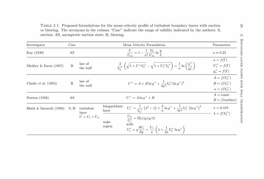
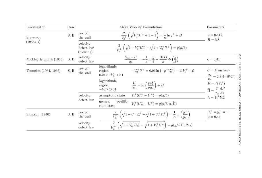
In the following paragraphs a review of the proposed mean-velocity scalings willbe given, while a summary is presented in Table 2.1.
For TASBLs, using Taylor’s vorticity-transfer theory and a mixing lengthdefined being proportional to the wall-normal distance L = κy, Kay (1948)obtained
U
U∞= 1− 1
κ2V0U∞
lny
δ, (2.17)
in which a logarithmic dependency of the streamwise velocity to the wall-normaldistance is observed. It should be noted that since this analysis is restricted toasymptotic suction cases, the proposed scaling extends until the boundary layeredge.
Rubesin (1954) was the first to apply Prandtl’s momentum-transfer theory tothe (compressible) boundary layer with blowing, deriving an integral expressionfor the near-wall turbulent region. For incompressible flow using L = κy asmixing-length, Prandtl’s momentum transfer theory gives
τ
ρ=
(κy∂U
∂y
)2
, (2.18)
which can be used in eq. (2.13) to obtain
u2τ + V0U =
(κy∂U
∂y
)2
. (2.19)
Eq. (2.19) can be rewritten as
u2τ + V0U =
[κ
V0
∂(u2τ + V0U)
∂ ln y
]2. (2.20)
The solution of this differential equation is
u2τ + V0U =V 20
4κ2(ln y + C1)2 , (2.21)
where C1 is an integration constant. One possible way to express eq. (2.21) inviscous scaling is (Stevenson 1963a)
2
V +0
(√1 + U+V +
0 − 1
)=
1
κln y+ + C2 −
2
V +0
, (2.22)

20 2. Boundary-layer flows with wall transpiration
where C2 = (C1 + ln `∗)/κ. Equation (2.22) reduces to the canonical logarithmiclaw of the wall (eq. 1.29) as long as
C2 → B +2
V +0
for V +0 → 0 , (2.23)
where B is the log-law intercept for the no-transpiration case. Stevenson (1963a)has however reported that the dependency on the transpiration rate of theterm C2 − 2/V +
0 is weak and he chose C2 − 2/V +0 = B for the description of all
his experimental results on blowing boundary layers. An expression similar toeq. (2.22) has been derived by many other authors (Clarke et al. 1955; Mickley& Davis 1957; Black & Sarnecki 1958; Stevenson 1963a; Simpson 1970), andhas recently been used by Kornilov (2015) to describe his experimental dataon turbulent boundary-layers with blowing. Rotta (1970) followed the sameprocedure, including a damping function following van Driest (1956) in orderto account for the viscous stresses near the wall. The difference between theexpressions proposed by the different authors is just in the values and in the wayof expressing the integration constant: a summary on the topic can be found inStevenson (1963a). As pointed out already by Rubesin (1954) and Clarke et al.(1955), both the mixing-length parameter κ and the integration constant shouldin general be regarded as functions of the suction or blowing rate. Nevertheless,it seems that all the supporters of the bilogarithmic law assumed the value of κto be constant or just weakly depending on the transpiration rate, fixing it tothe value for the turbulent boundary layer without mass transpiration. Mickley& Davis (1957), though, specified that “at values of V0/U∞ above 0.005 thevalue of κ increases with increasing values of V0/U∞”. The LHS of eq. (2.22)is sometimes referred to as the pseudo-velocity : if the mixing length parameterκ is independent of the transpiration parameter, a semilogarithmic plot of thepseudo-velocity against the wall-normal distance for the inner turbulent regionof boundary layers with mass transfer should result in a series of parallel lines.The bilogarithmic law has also been derived through an analytical approach byVigdorovich (2004), Vigdorovich & Oberlack (2008) and Vigdorovich (2016).
The application of momentum transfer theory to boundary-layer flows withmass transfer and the resulting bilogarithmic law appears to be the predominantview for the first decade of research on the topic. Doubts about the applicationof the mixing-length model to boundary-layer flows with mass transfer wereraised in Tennekes (1964) and Tennekes & Lumley (1972), stating in the latterthat “mixing-length models are incapable of describing turbulent flows containingmore than one characteristic velocity with any degree of consistency”. Mickley& Smith (1963) were the first to propose an alternative scaling, extending Coles(1956) decomposition of the canonical turbulent boundary-layer eq.(1.36) toboundary layers with wall transpiration and suggesting an empirical velocity-defect law of the form
U∞ − Uu∗τ
= − 1
κlny
δ+
Π(x)
κW(yδ
), (2.24)

2.2. Turbulent boundary layers with transpiration 21
where a dependency on the first power of the logarithm is evident. In eq. (2.24)u∗τ is a characteristic shear velocity based on the maximum shear stress. Con-sidering a boundary-layer flow without pressure gradient, the maximum shearstress does not coincide with the wall shear stress just in presence of blowing,while for the suction case eq. (2.24) would revert to the common velocity defectlaw for flows on non permeable surfaces, as long as κ is taken as constant.Tennekes (1964, 1965), Coles (1971) and Andersen et al. (1972) also suggested adependency of the streamwise velocity to the first power of the logarithm of thewall normal distance. Their rationale is that in presence of mass transfer it ispossible to adopt the same type of argument used by Millikan (1938) to derivethe log-law for turbulent boundary-layer flow on impermeable surfaces. Theboundary layer can be divided in a wall region which can be described with alaw of the wall
U
u0= f
(y
`0
), (2.25)
and an outer region where the velocity profile has the form of a defect law
U∞ − Uu0
= g(yδ
). (2.26)
The two regions share the same velocity scale u0, which can be related to thecharacteristic stress level close to the wall. If there is an overlap region whereboth descriptions are valid, then the velocity profile must have the logarithmicshape
U
u0=
1
κln
y
y0+B2 , (2.27)
or, equivalently,
U∞ − Uu0
= − 1
κlny
δ+B3 . (2.28)
For the case of a turbulent boundary layer flow without wall-normal masstransfer (see §1.3),
u0 = uτ =
√τwρ
and `0 = `∗ =ν
uτ. (2.29)
In presence of mass transfer, instead, since the viscous sublayer is described byeq. (2.16), an attractive choice of velocity and length scale is (Tennekes 1965)
u0 =τw/ρ
V0=u2τV0
and `0 =ν
V0, (2.30)
so that eq. (2.16) can be written in the form of eq. (2.25) as
U
u0= ey/`0 − 1 , (2.31)
independently of the suction ratio. If this choice of velocity scale proves to becorrect also for the outer part of the boundary layer, so that the velocity profile iscorrectly represented by eq. (2.26), then a logarithmic profile is expected to hold
22 2. Boundary-layer flows with wall transpiration
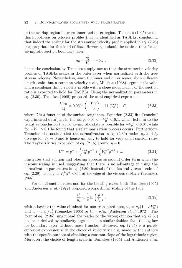
in the overlap region between inner and outer region. Tennekes (1965) testedthis hypothesis on velocity profiles that he identified as TASBLs, concludingthat indeed the scaling for the streamwise velocity profile applied in eq. (2.26)is appropriate for this kind of flow. However, it should be noticed that for anasymptotic suction boundary layer
u0 =u2τV0
= −U∞ , (2.32)
hence the conclusion by Tennekes simply means that the streamwise velocityprofiles of TASBLs scales in the outer layer when normalized with the free-stream velocity. Nevertheless, since the inner and outer region show differentlength scales but a common velocity scale, Millikan (1938) argument is validand a semilogarithmic velocity profile with a slope independent of the suctionratio is expected to hold for TASBLs. Using the normalization parameters ineq. (2.30), Tennekes (1965) proposed the semi-empirical expression
− UV0u2τ
= 0.06 ln
(−V0y
ν
)− 11
(V +0
)+ C , (2.33)
where C is a function of the surface roughness. Equation (2.33) fits Tennekes’experimental data just in the range 0.04 < −V +
0 < 0.1, which led him to thetentative conclusion that no asymptotic state is possible for −V +
0 < 0.04, whilefor −V +
0 > 0.1 he found that a relaminarization process occurs. FurthermoreTennekes also noticed that the normalization in eq. (2.30) makes u0 and `0diverge for V0 → 0 and is hence unlikely to hold for very small suction rates.The Taylor’s series expansion of eq. (2.16) around y = 0
U+ = y+ +1
2V +0 y
+2 +1
6V +20 y+3 + ... (2.34)
illustrates that suction and blowing appears as second order term when theviscous scaling is used, suggesting that there is no advantage in using thenormalization parameters in eq. (2.30) instead of the classical viscous scales ofeq. (2.29), as long as V +
0 y+ << 1 at the edge of the viscous sublayer (Tennekes
1965).
For small suction rates and for the blowing cases, both Tennekes (1965)and Andersen et al. (1972) proposed a logarithmic scaling of the type
U
uc∝ 1
κln
(y
`c
), (2.35)
with κ having the value obtained for non-transpired case, uc = uτ (1 + αV +0 )
and `c = νuc/u2τ (Tennekes 1965) or `c = ν/uc (Andersen et al. 1972). The
form of eq. (2.35), might lead the reader to the wrong opinion that eq. (2.35)has been derived by similarity argument in a similar fashion than the log-lawfor boundary layer without mass transfer. However, eq. (2.35) is a purelyempirical expression with the choice of velocity scale uc made by the authorswith the specific purpose of obtaining a constant slope of the logarithmic region.Moreover, the choice of length scale in Tennekes (1965) and Andersen et al.

2.2. Turbulent boundary layers with transpiration 23
(1972) do not have any specific role in the description of the flow and weredefined by analogy with the length scale for a boundary layer with or withoutmass transfer respectively. As a result, it is not possible to express the viscoussublayer as U/uc = f(y/`c). Formulations of the type of eq. (2.35) are henceequivalent to the empirical log-law with modified coefficient of the type
U+ = A ln y+ +B , (2.36)
used by Dutton (1958) to fit his experimental data. Watts (1972) and Bobkeet al. (2016) also favours this empirical logarithmic scaling, with the coefficientsA and B being functions of the suction rate.
The outer region
Following Coles (1956), Black & Sarnecki (1958) proposed a description of theouter region of a turbulent boundary layer with transpiration by summing aninner velocity component Ui coinciding with the bilogarithmic law of the walland a wake component Uw negligible in the inner part of the boundary layer.Differently from Coles (1956) they did not use uτ as the single normalizationparameter for the wake function, suggesting instead the use of the local shearvelocity of the bilogarithmic law y∂Ui/∂y. Mickley & Smith (1963) proposedthe use of a velocity defect law (eq. 2.24) in which a Coles-type wake function isevident. Stevenson (1963b), instead, proposed an extension of the bilogarithmiclaw to the wake region as a velocity defect law in the form:
2
V +0
(√1 + V +
0 U+∞ −
√1 + V +
0 U+
)= g(y/δ) , (2.37)
which was adopted also by Simpson (1970).
Tennekes (1965), instead, proposed a velocity defect law for turbulentasymptotic states in the form
V +0 (U+
∞ − U+) = g(y/δ) . (2.38)
Generalizing eq. (2.38) for non-asymptotic suction or blowing boundary layerswith pressure gradient, he proposed the tentative expression
V +0 (U+
∞ − U+) = g(y/δ,Λ, Π) , (2.39)
where Λ is a transpiration parameter and Π is a pressure-gradient parameter.
More recently, Cal & Castillo (2005) extended to boundary layers withtranspiration and pressure gradient the use of the empirical scaling proposed byZagarola & Smits (1998b) for ZPG TBLs, concluding that “the dependencies onthe upstream conditions, pressure gradient, and the blowing parameter are nearlyremoved from the mean deficit profiles when normalized by the Zagarola-Smitsscaling U∞(δ∗/δ)”, even though differences are observed between the blowingand the suction cases. Kornilov & Boiko (2012) tested the Zagarola-Smits scalingon their experimental data on ZPG boundary layer with blowing, obtaining agood overlap among the measured mean-velocity profiles.
24
2.
Boundary-l
ayer
flow
sw
ith
wall
transp
iratio
nTable 2.1. Proposed formulations for the mean-velocity profile of turbulent boundary layers with suctionor blowing. The acronyms in the column “Case” indicate the range of validity indicated by the authors: S,suction; AS, asymptotic suction state; B, blowing.
Investigator Case Mean Velocity Formulation Parameters
Kay (1948) ASU
U∞= 1− 1
κ2
V0
U∞lny
δκ ≈ 0.23
Mickley & Davis (1957) Blaw ofthe wall
2
V +0
(√1 + U+V +
0 −√
1 + U+a V
+0
)=
1
κln
(y+
y+a
) κ = f(Γ)
U+a = f(Γ)
y+a = f(Γ)
Clarke et al. (1955) Blaw ofthe wall
U+ = A+B ln y+ +1
4κ2V +0 (ln y+)2
A = f(V +0 )
B = f(V +0 )
κ = f(V +0 )
Dutton (1958) AS U+ = A ln y+ +BA = const.
B = f(surface)
Black & Sarnecki (1958) S, B turbulentlayerU = Ui + Uw
bilogarithmiclayer
U+i =
1
V +0
(λ2 − 1
)+λ
κln y+ +
1
4κ2V +0
(ln y+
)2κ = 0.419
λ = f(V +0 )
wakeregion
UwU∗i
= Π(x)g (y/δ)
with
U∗i = y∂Ui∂y
=Uτκ
(λ+
1
2κV +0 ln y+
)
2.2
.T
urbulent
boundary
layers
wit
htransp
iratio
n25
Investigator Case Mean Velocity Formulation Parameters
Stevenson
(1963a,b)
S, Blaw ofthe wall
2
V +0
(√V +0 U
+ + 1− 1
)=
1
κln y+ +B κ = 0.419
B = 5.8velocitydefect law(blowing)
2
V +0
(√1 + V +
0 U+∞ −
√1 + V +
0 U+
)= g(y/δ)
Mickley & Smith (1963) S, Bvelocitydefect law
U∞ − Uu∗τ
= − 1
κlny
δ+
Π(x)
κW(yδ
)κ = 0.41
Tennekes (1964, 1965) S, Blaw ofthe wall
logarithmicregion0.04<−V +
0 <0.1−V +
0 U+ = 0.06 ln
(−y+V +
0
)− 11V +
0 + C C = f(surface)ucuτ
= 2.3(1+9V +0 )
B = f(V +0 )
Π =δ∗
τw
dP
dx
Λ = V +0 U
+∞
logarithmicregion−V +
0 <0.04
U
uc= ln
(yu2
τ
νuc
)+B
velocity
defect law
asymptotic state V +0 (U+
∞ − U+) = g(y/δ)
general equilib-rium state
V +0 (U+
∞ − U+) = g(y/δ,Λ, Π)
Simpson (1970) S, Blaw ofthe wall
2
V +0
(√1 + U+V +
0 −√
1 + U+a V
+0
)=
1
κln
(y+
y+a
)U+a = y+a = 11
κ = 0.44
velocitydefect law
2
V +0
(√1 + V +
0 U+∞ −
√1 + V +
0 U+
)= g(y/δ,Π,Reθ)

26
2.
Boundary-l
ayer
flow
sw
ith
wall
transp
iratio
n
Investigator Case Mean Velocity Formulation Parameters
Rotta (1970) S, B U+ =[f(y+, V +
0 ) + g(y/δ)] A = 13.6 + 12.4 e−10.75V +
0
κ = 0.4
law ofthe wall
U+ = f(y+, V +0 )
df
dy+=
2(1 + V +0 U
+)
1 +
√1 + 4κ2y+2(1 + V +
0 U+)
(1− e−y+
√1+V +
0 U+/A
)2
Andersen et al. (1972) S, Blaw ofthe wall
U
uc=
1
κln(yucν
)+B + 14
(uτuc− 1
) κ = 0.41
B = 5.0ucuτ
= 1 + 7.7V +0
Watts (1972) S U+ = A ln y+ +B
A = 1/0.4(1− 390Γ)
B = 7.5 +5.5
π×
arctan [2.2 (−Γ/0.0014− 1)]
Bobke et al. (2016) AS U+ = A ln y+ +BA = f(Γ)
B = f(Γ)
Vigdorovich (2016) Slaw ofthe wall
2
V +0
(√(1 + U+V +
0 )− 1
)=
1
κ
[ln y+ +B0 −B1V
+0 +O((V +
0 )2)]
+O((y+)−α)
κ = 0.41
B0 = 2.05
B1 = 2.157
y+ → +∞α > 0

2.2. Turbulent boundary layers with transpiration 27
2.2.5. Reynolds stresses
Dutton (1958) calculated the Reynolds shear stress u′v′ profile in an turbulentasymptotic suction boundary layer from the measured streamwise velocitygradient through eq. (2.13) with τ ≈ −ρu′v′, reporting a strong decrease of thepeak value of u′v′+ when suction was applied. He then used the calculatedReynolds shear stress and the measured velocity gradient to obtain an estimatefor the turbulence production and the viscous dissipation term of the mean-flowenergy equation, concluding that in presence of suction the larger velocitygradient at the wall enhances the viscous dissipation, decreasing the relativeamount of mean-flow energy transferred to the turbulent motion. Similar resultswere also obtained by Rotta (1970), who also included in the analysis boundarylayers with blowing, reporting a large increase of the near-wall turbulenceproduction term in presence of blowing.
To my knowledge, the first study reporting direct measurements of theReynolds stresses in boundary layers with suction is by Favre et al. (1961).
Profiles of u′2, v′2, and u′v′ were reported, concluding that in presence of suctionthe Reynolds stresses are damped in the whole boundary layer compared to theno-transpiration case. Favre et al. (1966) concluded the same behaviour also
for the spanwise component w′2. Similar results were obtained by Andersenet al. (1972), even if complicated by pressure gradient effects. The variouscomponents of the Reynolds stress tensor are affected differently by wall-suction,with the near-wall anisotropy increasing with the suction rate. This increasein anisotropy is explained by the increased organization of the near-wall flowshowing a “more orderly behavior of low-speed and high-speed streaks and agreater longitudinal coherence of the low-speed streaks” (Antonia et al. 1994).Fulachier et al. (1977) reported X-wire anemometry results showing that the
streamwise velocity variance u′2 was damped the most by the suction, while w′2
was affected the least, in agreement with Antonia et al. (1988) but in contrastwith Elena (1975) and Fulachier et al. (1982) (as reported by Antonia et al.
1988), who conjectured that w′2 should be more damped by the suction than u′2.Finally Antonia et al. (1994), analyzing the DNS simulation results by Marianiet al. (1993), concluded that the component of velocity fluctuation most affected
by suction was v′2, followed respectively by w′2 and u′2. These differencesbetween numerical and experimental results were explained by Antonia et al.(1994) with the difficulties in obtaining reliable measurements of the near-wallfluctuations with hot-wire anemometry through X- or V-probes.
The Reynolds stresses are magnified by wall-normal blowing, as observed inthe experimental data by Andersen et al. (1972) and Kornilov (2015) and in theLES by Kametani et al. (2015). In general blowing increases the magnitude ofthe Reynolds stresses particularly in the outer part of the boundary layer: in therange of blowing rate and Reθ explored by Andersen et al. (1972) a secondary
peak in the u′2 profiles emerges in the outer part of the boundary layer, whichin some case is larger in magnitude than the near-wall peak. For the blowing

28 2. Boundary-layer flows with wall transpiration
rate reported in Kornilov (2015) a single peak in the u′2 profiles located in theouter part of the boundary layer is observed. Since with increasing blowing thewall shear stress decreases (and hence the viscous length-scale increases), theseobservations cannot be explained by spatial filtering of the hot-wire probe.
The Reynolds shear-stress distribution in a TASBL
In the special case of the turbulent asymptotic suction boundary layers, it ispossible to derive a relation between the Reynolds shear-stress and the meanvelocity profile. As already noted above, for an asymptotic boundary layereq. (2.12) is exact. Dividing both sides of eq. (2.12) with the asymptotic wallshear stress τw = −ρU∞V0 we get
τ
τw= 1− U
U∞. (2.40)
For a turbulent boundary layer τ ≈ −ρu′v′ everywhere but in the near-wallregion, hence for a large portion of the boundary layer
− u′v′
u2τ≈ 1− U
U∞, (2.41)
relating the inner-scaled Reynolds shear stress to the outer-scaled mean velocityprofile.
Chapter 3
Experimental setup and measurementtechniques
This chapter presents a description of the experimental setup built for thisstudy together with a summary on the measurement techniques employed.The main component of the apparatus is a flat plate with a permeable topsurface installed in the Minimum Turbulence Level wind tunnel of the FluidPhysics Laboratory at the Department of Mechanics of KTH - Royal Instituteof Technology. A suction/blowing system providing the necessary air flowthrough the permeable surface and two automated traverse systems completethe apparatus. Each of these parts will be described in detail in the followingsections and the main design choices will be motivated. Thermal anemometryand oil-film interferometry will briefly be introduced and, finally, an account onthe measure of the wall shear stress on permeable surfaces with a miniaturizedPreston tube will be given.
3.1. Wind tunnel
The Minimum Turbulence Level (MTL) wind tunnel is a closed loop wind tunnelwith a 7 m long test section having a cross-sectional area of 1.2× 0.8 m2. Themaximum streamwise turbulence intensity for an empty test section in the speedrange from 10 m/s to 60 m/s is less than 0.04% and a cooling system maintainsthe temperature of the flow constant with a maximum variation around themean in space and time of ±0.07K. The adjustable shape of the ceiling and floorof the test section allows the regulation of the pressure gradient. The interestedreader can find more details on the wind-tunnel design and characteristics inJohansson (1992) and Lindgren & Johansson (2002).
3.1.1. Test-section modifications
Considerable modifications to the wind-tunnel test section were required toallow the desired installation of the present experimental apparatus. In pres-ence of wall suction/blowing over a large area of a wind-tunnel model, thesignificant ejection/injection of mass flow from the test section results in anacceleration/deceleration of the flow along the streamwise direction. In orderto compensate for this effect, the ceiling, originally made of 30 mm thick wood
29

30
3.
Experim
ental
setup
and
measu
rem
ent
techniq
ues
650(c)
(a)
(d)
(e)(f)
(b)
Figure 3.1. Drawing of the experimental setup mounted in the MTL wind-tunnel test section. Filledareas: Perforated surfaces; (a) Impermeable leading-edge section; (b) leading-edge bleed slot; (c) Landingtraverse system (x− y); (d) Ceiling-height adjustment station; (e) Wall-mounted traverse system; (f ) Oil-filmmeasurement station. Note: The Landing traverse system was unmounted when performing oil-film orhot-wire measurements at the downstream station (e, f ).

3.1. Wind tunnel 31
panels, was exchanged with a series of perforated steel sheets with hole diame-ter 2 mm and a hole spacing giving an open area of 29.6%. The idea behindadopting this largely perforated ceiling, was to impose constant static pressurealong the whole test section, thus obtaining a zero-pressure-gradient boundarylayer on the test surface. However, when the wind tunnel was run with the newceiling, very large velocity fluctuations were observed, originating from the flowbeing alternately discharged through the ceiling or through the wind-tunneldiffuser. The solution of the problem was found by covering a large extent ofthe perforated area of the ceiling with adhesive plastic foil, leaving just 100 mmlong open slots every 1 m. Apart from the ejection/injection effect, the flowaccelerates inside the test section due to the growth of the boundary layers onall the walls. This effect is typically taken care of by adjusting the shape of theceiling such that the total cross-sectional area of the test section increases withthe downstream distance. Preliminary experiments showed however that theopen area of the ceiling together with the largest allowed regulation of the shapeof the ceiling was not sufficient to obtain a ZPG region extending over the wholestreamwise length of the test plate. The problem was solved installing a 1.2 mlong wall liner inside the wind-tunnel contraction section with the function todecrease the inlet cross-sectional height of the test section to 0.7 m from theoriginal 0.8 m and, hence, allowing a larger expansion of the cross-sectionalarea. With this configuration a large ZPG region could be obtained for anyexperimental condition examined through a joint regulation of the ceiling shapeand of a bleed-slot opening beneath the plate leading edge (see §3.2.1 for moredetails). The pressure gradient was checked either with a hot-wire traverseor with pressure-taps readings before each measurement and a regulation ofthe ceiling shape and/or of the bleed-slot opening was performed wheneverneeded. With this procedure the variation of U∞ was typically limited to lessthan ±0.5% on the whole plate model, with somewhat larger variation limitedto the first meter from the leading edge.
The test-section modifications described above and the installation of theplate model increased the free-stream disturbance level compared to the originalempty test section. The streamwise turbulence intensity in the free-streamincreases along the streamwise direction, reaching a maximum level of 0.2% atthe most downstream measurement location (6.06 m downstream of the leadingedge).
3.1.2. Traverse system
The MTL wind tunnel can be equipped with a fully automatic 5-axis traversesystem, able to accurately position a probe mounted on a sting penetrating intothe test section from a slot in the middle of the ceiling. At the flow velocityconsidered in this investigation (up to 45 m/s), flow-induced vibrations on thesting would cause erroneous data and frequent hot-wire probe breakage in closeproximity to the wall. In order to reduce probe vibrations, a new traversesystem was designed such that the traverse arm could be supported by the plate,

32 3. Experimental setup and measurement techniques
92
204 345
397
(a)
(b)
(c)
(d) (e)
(f)(g)
(h)
I.
II.
x
y
x
y
Figure 3.2. Drawing of the Landing traverse system. I. LiftedSecondary stage; II. Landed secondary stage. (a) vertical stingtraversable in the x− y direction from the main wind-tunneltraverse; (b) rotating shaft; (c) spring: (d) rubber feet; (e)wheel; (f ) DC servomotor; (g) stop switch; (h) hot-wire probe.
instead of simply hanging from the ceiling. Figure 3.2 reports a drawing of thisnew traverse system, which will in the following be referred to as the Landingtraverse system. It is made of two main components, a wing-shaped verticalsting (a), which is attached to the main traverse chassis on the top of thetest-section, and a secondary traverse stage pivoting around a small shaft (b).

3.2. Perforated flat plate 33
The vertical wing can be moved in the streamwise and wall-normal direction bythe main wind-tunnel traverse system. A motion routine starts with raising thevertical sting until the secondary stage is lifted from the surface, as indicatedin Figure 3.2I. The vertical wing is then moved in the desired streamwise xlocation and lowered toward the surface, with the wheel (e) facilitating themotion of the secondary stage on the surface. The vertical motion is interruptedby the electrical switch (g), regulated so that it activates when the rubber feet(d) touches the surface. The secondary stage is now pressed in position on theplate by a spring (c) as depicted in Figure 3.2II. Finally the desired positionof the probe (h) is adjusted rotating a leadscrew with the DC servomotor (f ).The servomotor is equipped with a rotary encoder ensuring a relative accuracyof the vertical displacement of the probe of ±1 µm. The vertical range of thesecondary traverse stage, and hence of the probe, is 180 mm. The extent ofthe upstream region influenced by the traverse system was checked moving thetraverse system progressively closer to a fixed Prandtl tube. The length of thehorizontal sting supporting the probe was then chosen such that the deviationin velocity measured by a Prandtl tube was less than 0.5% from the undisturbedvalue.
3.2. Perforated flat plate
3.2.1. Design and construction
A drawing of the flat plate installed inside the wind-tunnel test section is shownin Figure 3.1. The flat plate is 6.6 m long and spans the whole 1.2 m width of thewind-tunnel test section. It starts with a 122 mm long impermeable ellipticalleading edge followed by 8 individual plate elements, each one extending 812 mmin the streamwise direction. Finally, a 1.2 m long linear diffuser (not shownin Fig. 3.1) extends inside the wind-tunnel diffuser section from the platetrailing edge, expanding the flow to the full local cross-sectional area. Theplate is installed in the test section such that the test surface constitutes thewind-tunnel bottom surface. Such arrangement was preferred to the morecommon installation of the flat plate in the mid-height of the test-section fortwo reasons: first, the extra blockage originating from the suction/blowingtubing was deemed problematic, moreover since this configuration maximizesthe distance between test-section floor and ceiling, it guarantees a larger regionof free stream reducing blockage effects. In order to remove the boundarylayer developed in the wind-tunnel contraction and to allow the developmentof a fresh boundary layer with a well-defined origin on the test plate, the flowbeneath the plate leading edge is vented through a bleed slot with an adjustableopening (see Fig. 3.3). Thirteen pressure taps allow the measurement of thepressure distribution on the leading-edge top and bottom surface.
The variation of the leading-edge pressure coefficient as function of thebleed-slot opening is illustrated in Figure 3.4b, showing that quite a largeregulation is possible with the permissible adjustment of the bleed-slot opening.Figure 3.4a show instead the variation of the leading-edge pressure distribution

34 3. Experimental setup and measurement techniques
345
h o = 2
5 ÷
50
285
280
23
26
(b)(a)
122
03
1020
4080120
122
26
Ø 0.5
Figure 3.3. Top: Detail view of the leading-edge bleed slot.The right edge of the drawing corresponds to the start ofthe test-section. A hinged surface (a) allows the adjustmentof the bleed-slot opening (ho) through the regulation of twoturnbuckles (b). Bottom: Magnified view of the ellipticalleading edge with its pressure taps.
at fixed bleed-slot opening but varying free-stream velocity, showing that aregulation of the bleed-slot opening is needed in order to maintain a fixedleading-edge pressure distribution at different experimental conditions. Thepossibility of using an active venting system for the regulation of the leading-edge pressure coefficient was explored during the preliminary design of thecurrent experimental apparatus and is described in Ferro et al. (2015).
Each individual plate element is a sandwich construction: a 0.9 mm thickperforated titanium sheet is glued on a frame of square, L- and T-beams boltedon a 6 mm thick bottom plate (see Fig. 3.5 and 3.6). The T-beams elongatein the spanwise direction, with a streamwise spacing of 57.5 mm, chosen tolimit the maximum plate deflection at the maximum suction level to less than5 µm (calculated with classical beam theory). The webs of the T-beams areperforated to ensure a uniform pressure in the plate inner chamber. The widthof the webs of the L- and T-beams was chosen to be 2 mm to minimize the

3.2. Perforated flat plate 35
0 20 40 60 80 100 120
−1
−0.5
0
0.5
1
Cp
x (mm)
h
o = 30 mm(a)
U∞
= 15.0 m/s
U∞
= 20.0 m/s
U∞
= 30.0 m/s
U∞
= 40.0 m/s
0 20 40 60 80 100 120
−1
−0.5
0
0.5
1
Cp
x (mm)
U
∞
= 20 m/s(b)
ho = 25 mm
ho = 30 mm
ho = 35 mm
ho = 40 mm
ho = 45 mm
ho = 50 mm
Figure 3.4. Leading-edge pressure coefficient. (a): fixedbleed-slot opening (ho) and varying free-stream velocity; (b):fixed free-stream velocity and varying bleed-slot opening.
streamwise direction where suction/blowing is interrupted, while providingsufficient surface for the glue to hold. In each plate an access port for a 10 mmdiameter cylindrical plug is provided. Originally conceived for hot-film wall-shear-stress measurements, the plugs were instead mainly used to host pressuretaps for measuring the streamwise pressure gradient. Inside each plate fourpressure taps measure the static pressure in the inner chamber: in order tocheck the pressure uniformity, two of these pressure taps are located close to thecentre of the plate, while the other two are located 25 mm from the edges of theplate in two opposite corners. The titanium sheets (provided by CAV AdvancedTechonologies in Consett, UK) are laser drilled with 64 µm diameter holes witha centre-to-centre spacing of 0.75 mm in both spanwise and streamwise direction,giving a total open area of 0.56%. The holes are not aligned in the streamwisedirection, but rather a random pattern with fixed centre-to-centre distance andfixed row spacing was chosen, in order not to introduce any preferential spanwisescale in the flow. Since smoothness at the joint is important, the titaniumsheets were designed 2 mm shorter than the frame, so that a gap originatesbetween two adjacent plates on assembly. This gap is then filled with boxing
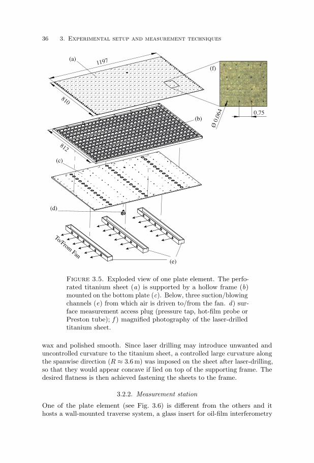
36 3. Experimental setup and measurement techniques
To/From Fan(e)
(d)
(c)
(f)(a)
(b)
812
1197
0,75
Ø 0
,064
810
Figure 3.5. Exploded view of one plate element. The perfo-rated titanium sheet (a) is supported by a hollow frame (b)mounted on the bottom plate (c). Below, three suction/blowingchannels (e) from which air is driven to/from the fan. d) sur-face measurement access plug (pressure tap, hot-film probe orPreston tube); f ) magnified photography of the laser-drilledtitanium sheet.
wax and polished smooth. Since laser drilling may introduce unwanted anduncontrolled curvature to the titanium sheet, a controlled large curvature alongthe spanwise direction (R ≈ 3.6 m) was imposed on the sheet after laser-drilling,so that they would appear concave if lied on top of the supporting frame. Thedesired flatness is then achieved fastening the sheets to the frame.
3.2.2. Measurement station
One of the plate element (see Fig. 3.6) is different from the others and ithosts a wall-mounted traverse system, a glass insert for oil-film interferometry

3.2
.P
erforated
flat
plate
37
57,5
130150
58
26Ø 40
Figure 3.6. The most downstream plate element with the wall-mounted traverse system, the oil-filminterferometry measurement station and the surface measurement access plug.

38 3. Experimental setup and measurement techniques
Figure 3.7. Photography depicting the bottom side of theplate, with the suction/blowing channel and the flexible hoses.
skin-friction measurements and the 10 mm diameter plug also present in theother plate elements. In order to avoid leakage when suction/blowing is applied,the oil-film-interferometry plug, the access plug and the traverse system aremounted into sleeves protruding in the inner chamber of the plate. This platewas mounted in the most downstream position, so that the wall-mounted traverseallows the measurement of boundary-layer profiles in a location unaccessibleto the wind-tunnel traverse system. The traverse has a range of 500 mm and arelative accuracy of ±1 µm. The positioning is obtained with a DC servomotorcontrolled with a rotary optical encoder. Since the traverse is fixed to the plateand the traverse mechanism is not exposed to the flow, probe vibrations arekept at a minimum.
3.3. Suction/blowing system
The suction/blowing system is the system of hoses, valves and a fan whichallows to generate and regulate the airflow through the perforated plate. Foreach plate section eighteen flexible hoses with a diameter of 25 mm depart fromthe side of the three suction channels on the bottom side of the plate (seeFig. 3.7). These flexible hoses are connected to 8 manifolds (one for each plate)from which rigid steel pipes 125 mm in diameter drive the flow to a woodensuction chamber (see Fig. 3.8). Eight regulation valves allow the adjustment ofthe volume flow in each one of the steel pipe, so that a uniform transpirationvelocity can be ensured even in presence of differences in the permeability ofeach titanium sheet. The chamber is connected to a 7.5 kW AC centrifugal fanthrough a single pipe 200 mm in diameter equipped with a flowmeter measuring

3.5. Hot-wire anemometry 39
the total volume flow driven by the system. The regulation of the volume flowis obtained adjusting the fan rotation speed with a variable-frequency drive.
3.4. Instrumentation
3.4.1. Air properties
The atmospheric pressure Patm was measured with a Druck PTX 520 absolutepressure transmitter (accuracy of ±180 Pa) connected to a Furness FCO510micromanometer. The air temperature T was obtained measuring with a Fluke-45 multimeter the resistance of Pt-100 sensor positioned in proximity of thehot-wire probe. The estimated accuracy on the temperature is ±0.15 K. Airdensity is obtained from the ideal gas law
Patm = ρRT , (3.1)
where the specific gas constant is R = 287 J kg−1 K−1. The dynamic air viscositywas obtained from Sutherland’s formula
µ
µ0=
T
T0
3/2T0 + S
T + S, (3.2)
with constants S = 111 K, T0 = 273 K and µ0 = 1.716× 10⁻⁵ (constants fromWhite 1991).
3.4.2. Differential pressure measurements
Dynamic pressure
The dynamic pressure in the free stream was measured with a Prandtl tubeand monitored during the experiments. The Prandtl tube was also used as thereference for the calibration of the hot-wire probes. The differential pressurebetween the total and static port was measured with a Furness FCO510 pressuretransducer with an accuracy of ±0.25% of the reading for differential pressuresfrom 20 Pa to 2000 Pa and of ±0.05 Pa for differential pressures smaller than20 Pa.
Static pressure taps
The pressure taps on the surface of the plate, the leading-edge pressure taps andthe pressure ports inside the plate chamber were monitored with a 16 inputsScanivalve DSA 3217 with a nominal accuracy of ±5 Pa. Given the limitedamount of pressure inputs available on the pressure transducer, not all thepressure taps can be measured simultaneously but a choice was made accordingto the specific measurement requirements.
3.5. Hot-wire anemometry
3.5.1. Introduction
Due to the small length scale and time scale encountered in the investigated flowcases, with the viscous length scale as small as l∗ ≈ 6 µm for some turbulent

40 3. Experimental setup and measurement techniques
(d)
(a)
(b)
(c)
Figure 3.8. Photography of a portion of the suction/blowingsystem. The wind-tunnel test section is on the left of the photo.(a) manifold; (b) regulation valve; (c) suction/blowing chamber;(d) centrifugal fan.

3.5. Hot-wire anemometry 41
suction boundary layers, the most suitable measurement technique is hot-wireanemometry. Hot-wire (and hot-film) anemometry relies on the dependence ofthe heat transfer from a heated surface on the fluid motion of the surroundingfluid. In practice, Joule heating is used to heat an electrically conductingelement which is simultaneously cooled by a fluid stream. An electrical circuitmeasures the changes in electrical resistance of the sensor, which are related toits temperature variation and in turn to the fluid velocity. The way the electricalcircuit is designed differentiates the Constant Current Anemometry (CCA),the Constant Voltage Anemometry (CVA) and the Constant TemperatureAnemometry (CTA), which was used for this investigation. If the heated sensorhas the shape of a wire suspended between two conducting support (prongs)it is referred to as hot-wire, if it has the shape of thin film deposited on ainsulating substrate it is called hot-film. Hot-wire are the preferred choice formeasurements in gasses, while hot-film are used in liquids or for wall-shear-stressmeasurements. A common choice for the material of hot-wire and hot-filmprobes is tungsten, or platinum and its alloys. The diameter of a hot-wire isusually in the order of 1 µm to 5 µm and its length ranges from 0.25 mm to 2 mm,with the length over diameter ratio lw/dw ' 200 in order to limit the magnitudeof the conductive heat transfer to the prongs (Ligrani & Bradshaw 1987), whichdegrades the time-response of the sensor. Measurements of multiple velocitycomponents and of flow vorticity are also possible if multiple wires are used.The small physical dimension of the probe makes the frequency response oftypical hot-wires much faster than other measurement techniques, ranging inthe order of tens of kilohertz, a characteristics that make hot-wire anemometrywell-suited for measurements in turbulent or unsteady flows. However spatialresolution, due to the size of the sensing element, can become a limitationfor hot-wire measurements (as for any other measurement technique) in highReynolds number turbulent flows. For this reason efforts to build nanoscalesensing element have been initiated in the last decade, leading to the productionof the NanoScale Thermal Anemometry Probe (NSTAP) (see e.g. Fan et al.2015). Since hot-wire anemometry has been a commonly used measurementtechnique for more than a century, the literature on the topic is rich and theinterested reader is referred to the textbooks by Perry (1982), Lomas (1985),Bruun (1995) and Tropea et al. (2007, §5.2).
3.5.2. Sensors characteristics
In this investigation in-house built boundary-layer type single-wire probes wereused and an account on the manufacturing process can be found in Ferro (2012).The wires were made out of platinum, which is commercially available in theform of Wollastone wire (a platinum wire clad in silver). For probes withwire-length Lw > 0.5 mm, wires with diameter dw = 2.54 µm were used. In thiscase the Wollastone wire was immersed in nitric acid to fully remove the silvercoating, then the platinum core was directly soldered on the prongs. Probeswith Lw < 0.5 mm required instead the use of a thinner wire with diameterdw = 1.27 µm: in this case the un-etched Wollastone wire was soldered on the

42 3. Experimental setup and measurement techniques
(a) (b)
6 V
H2NO3(6% m/m)
1 mm
Figure 3.9. Photography of the Wollastone wire electroetch-ing (a) and of the finished hot-wire probe (b).
prongs, spaced of approximately 1 mm, and the platinum core was exposed forthe desired length by electroetching with a small jet (dj = 0.15 mm) of dilutednitric acid (see Westphal et al. 1988), as shown in Figure 3.9.
3.5.3. Sensors operation and calibration procedure
The hot-wire probes were operated in constant temperature mode with aDantec StreamLine 90N10 frame in conjunction with a 90C10 CTA module.The resistance overheat OH was set to 70% or 80%, with
OH =Rh −Rc
Rc, (3.3)
where Rh indicates the electrical resistance of the sensor at operating tempera-ture and Rc the resistance at flow temperature. For probes with dw = 2.54 µm,the square-wave test gave a frequency response between 35 kHz to 85 kHz atflow velocities from 0 m/s to 45 m/s. In these cases an analogue low-pass fil-ter with 30 kHz cut-off frequency was applied on the signal. For probes withdw = 1.27 µm the square-wave test gave a frequency response between 85 kHzto 150 kHz at flow velocities from 0 m/s to 40 m/s and the low-pass filter cut-offfrequency was set to 100 kHz. The hot-wire signal was amplified and finallyacquired with a 16bit National Instruments PCI-6259 acquisition card.
The probes were calibrated in-situ in the free stream against a Prandtl tubeconnected to a Furness FCO510 pressure transducer. The number of calibrationpoints varied between 12 and 20, increasing for larger velocity ranges, withthe lowest velocity point having a speed U ≈ 1.4 m/s. Below this speed thesteady operation of the tunnel and the accuracy in the differential pressuredetermination cannot be guaranteed in the present setup. At lower velocity thetunnel cannot be maintained at constant temperature, and the measurement

3.6. Transpiration velocity determination 43
0.45 0.5 0.55 0.6 0.650
5
10
15
20
25
30
35
40
E (V)
U (
m/s
)
pre−calibration
post−calibration
calibration law
Figure 3.10. Typical pre- and post-calibration of one of ahot-wire probes used for the experiments.
uncertainty on the differential pressure measured at the Prandtl tube portbecomes larger. A fourth order polynomial fit through the calibration points(including the hot-wire signal at zero velocity, E0) was used as calibrationlaw. The flow temperature was kept the same between calibration and mea-surements, hence no temperature correction of the measured data is required.The calibration procedure was repeated many times in one day in order tocheck for calibration drift. While for probes with wire diameter dw = 2.54 µmthe calibration law appeared to be very stable in time, it was observed thatprobes with wires with diameter dw = 1.27 µm were more prone to show driftproblems, as already reported by Hites (1997) and Discetti & Ianiro (2017).When these probes were in use, a full calibration was performed before and aftereach boundary-layer profile measurement and the hot-wire signal at a referencelocation in the free stream was acquired several times during the experimentto check and quantify the possible drift. The calibration law used for theseexperiments has been obtained from interpolated calibration points, average ofthe pre- and post-calibration laws (see Fig. 3.10). The largest variation in themeasured free-stream velocity between the start and the end of the measurementhas been 1.4%, even though for most of the cases the variation was limited toless than 1%.
3.6. Transpiration velocity determination
Two different methods were used to determine the transpiration velocity. Thetotal volume flow through the eight plates was measured with a flow meterduring all the experiments and could be related to the mean transpirationvelocity on the whole plate. Moreover the differential pressure across thetitanium sheets was monitored and, in combination with previously determined

44 3. Experimental setup and measurement techniques
0 200 400 600 800 10000
0.05
0.1
0.15
0.2
∆P (Pa)
|V0|(m/s)
T = 295.1 K P
atm = 100.9 kPa
(a)
20 40 60 80 100 1201
2
3
4
5
6
7
dh
√ρ∆P
µ
|V0|×
103
√∆P/ρ
(b)
Figure 3.11. Suction velocity V0 vs. the differential pressureacross the titanium sheet ∆P for all the eight plate elementexpressed in physical units (a) and normalized form (b). Thesolid line are third-order polynomial fit thorugh the measuredpoints.
plate permeability, it can be related to the transpiration velocity through eachplate element. The flow meter used was a Lindab FMU-200 nozzle-type flowmeter, specifically calibrated for this experiment with extended uncertainty of±1.5%.
The permeability of each assembled plate element for the cases of suctionand blowing was determined applying suction and blowing to one plate at atime while measuring the total flow rate and the pressure drop (∆P ) acrossthe sheet. The uniformity of the pressure in the chamber of the plate couldbe checked comparing the pressure measured at four different locations (see§3.2.1) and the variation was found to be less than ±1%. The volume flowrate was measured with a Meriam 50MC2-6 laminar flow element (accuracy±1.5%) and could directly be related to the suction/blowing velocity (V0).The results for the suction case are reported in Figure 3.11 for all the eightplates. The use of the two normalized parameters dh
√ρ∆P/µ (where dh is the
diameter of one hole) and |V0|/√
∆P/ρ allows to compensate for the variationof ambient condition between the permeability measurement and the actualexperiments. A third order polynomial fit through the measured points is usedto calculate the vertical velocity from the measured ∆P , ρ and µ. Plate-to-platevariation can be observed from Figure 3.11 and concerns on the uniformityof the permeability of each plate were raised. Due to the impossibility ofmeasuring the local permeability on the whole 7.5 m2 of perforated surface,permeability measurements were performed on four circular samples of diameter60 mm obtained from a 150 mm× 150 mm test piece manufactured in the same

3.7. Skin-friction measurement 45
0 100 200 300 400 5000
0.02
0.04
0.06
0.08
0.1
0.12
0.14
∆P (Pa)
|V0| (m
/s)
Figure 3.12. Suction velocity V0 vs. the differential pressureacross the titanium sheet ∆P for four samples obtained froma single test piece.
way as the eight larger sheets used in the plate elements. The results areshown in Figure 3.12 and the uniform behaviour of the different samples can beobserved. As a conclusion, the plate-to-plate variation in permeability observedin Figure 3.11 is likely due to a systematic variation of the mean hole size amongthe different sheets, which were not laser drilled in a single batch but one by one.Since the permeability of each plate is known, a uniform suction velocity on thewhole perforated surface can be obtained regulating the differential pressureacross each of the eight sheets with the regulation valves of the suction/blowingsystem (see §3.3). The valves need to be regulated for each transpiration velocity,and, of course, whenever a portion of a plate is covered to partially reduce thesuction area. With this procedure a deviation of the suction velocity smallerthan ±2.5% could be obtained between the different plate elements.
During the experimental campaign an increasing deviation between thesuction velocity measured from the differential pressure across the sheets andthe one measured with the flow meter was observed. Cleaning the surfacewith acetone strongly reduced the discrepancies, hence it was concluded thatthe cause for the deviation had been the deposition of dust and dirt on theplate surface. For this reason the suction velocity used for the data analysiswas obtained from the flow-meter measurements, which measure directly thevolume flow rate, while the differential pressure measurements have been usedexclusively to check and regulate the uniformity of the suction velocity betweenthe different plate elements.
3.7. Skin-friction measurement
In boundary-layer studies the wall shear stress is a quantity of great importance.As a measure of the forces exchanged between the flow and an object, it capturesthe results of all the physical phenomena occurring in the boundary layer. For

46 3. Experimental setup and measurement techniques
U
α
oil
Figure 3.13. Schematics of the oil-film interferometry workingprinciple. The incident light must be monochromatic.
this reason, in addition to the obvious practical relevance for engineeringapplications, it has a fundamental role in the theoretical description of turbulentboundary layers, often as a scaling parameter in the form of uτ . For turbulentboundary layers on impermeable surfaces, oil-film interferometry has in thelast decade become one of the reference techniques to measure the wall shearstress. However, since it relies on the observation of the motion of a thin filmof oil on a surface, it cannot be used on permeable surfaces. As a result, in thisinvestigation oil-film interferometry has been employed exclusively for the caseof canonical turbulent boundary layer. Measuring shear stress on permeablesurfaces present significant challenges: efforts to use hot-films or miniaturizedPreston tube for shear-stress measurement on permeable surfaces were initiated,but proved to be unsuccessful. Few attempts of measuring wall shear stressover permeable surfaces with floating elements with a porous surface can befound in the literature (Dershin et al. 1967; Depooter et al. 1977). However, thetechnological difficulties in realizing such a balance (especially for the necessityof an air-tight but mechanically isolated air supply) and the problematics relatedto the errors originating from misalignements and gap-sizes discouraged theauthor from the use of this technique.
The following section will report a brief summary on the theory of oil-filminterferometry together with details on the specific experimental arrangement.Next, the attempts to use a hot-film probe and a miniaturized Preston tube forthe determination of shear stress on porous surfaces are documented.
3.7.1. Oil-film interferometry
Oil-film interferometry is a technique which allows the direct measurement ofthe mean wall shear stress through the observation of the motion of a very thinlayer of oil (< 10 µm) deposited on a surface and stretched by the action ofthe flow. The local thickness of the oil film is visualized and made measurableby the use of Fizeau interferometry. This technique was first introduced byTanner & Blows (1976) and further developed by Monson (1983) and Zilliac(1996) among others. Its evolution has been strictly related to the technological
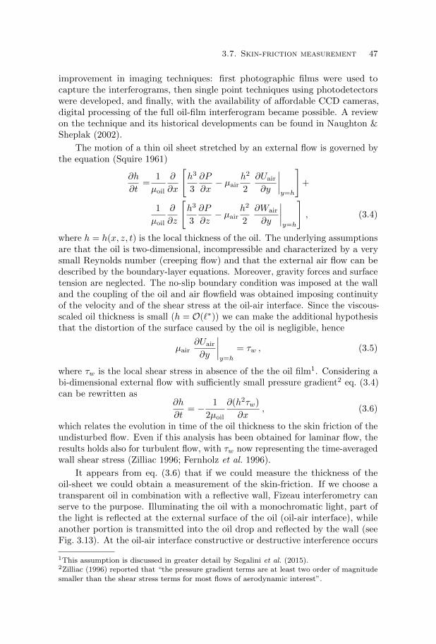
3.7. Skin-friction measurement 47
improvement in imaging techniques: first photographic films were used tocapture the interferograms, then single point techniques using photodetectorswere developed, and finally, with the availability of affordable CCD cameras,digital processing of the full oil-film interferogram became possible. A reviewon the technique and its historical developments can be found in Naughton &Sheplak (2002).
The motion of a thin oil sheet stretched by an external flow is governed bythe equation (Squire 1961)
∂h
∂t=
1
µoil
∂
∂x
[h3
3
∂P
∂x− µair
h2
2
∂Uair
∂y
∣∣∣∣y=h
]+
1
µoil
∂
∂z
[h3
3
∂P
∂z− µair
h2
2
∂Wair
∂y
∣∣∣∣y=h
], (3.4)
where h = h(x, z, t) is the local thickness of the oil. The underlying assumptionsare that the oil is two-dimensional, incompressible and characterized by a verysmall Reynolds number (creeping flow) and that the external air flow can bedescribed by the boundary-layer equations. Moreover, gravity forces and surfacetension are neglected. The no-slip boundary condition was imposed at the walland the coupling of the oil and air flowfield was obtained imposing continuityof the velocity and of the shear stress at the oil-air interface. Since the viscous-scaled oil thickness is small (h = O(`∗)) we can make the additional hypothesisthat the distortion of the surface caused by the oil is negligible, hence
µair∂Uair
∂y
∣∣∣∣y=h
= τw , (3.5)
where τw is the local shear stress in absence of the the oil film1. Considering abi-dimensional external flow with sufficiently small pressure gradient2 eq. (3.4)can be rewritten as
∂h
∂t= − 1
2µoil
∂(h2τw)
∂x, (3.6)
which relates the evolution in time of the oil thickness to the skin friction of theundisturbed flow. Even if this analysis has been obtained for laminar flow, theresults holds also for turbulent flow, with τw now representing the time-averagedwall shear stress (Zilliac 1996; Fernholz et al. 1996).
It appears from eq. (3.6) that if we could measure the thickness of theoil-sheet we could obtain a measurement of the skin-friction. If we choose atransparent oil in combination with a reflective wall, Fizeau interferometry canserve to the purpose. Illuminating the oil with a monochromatic light, part ofthe light is reflected at the external surface of the oil (oil-air interface), whileanother portion is transmitted into the oil drop and reflected by the wall (seeFig. 3.13). At the oil-air interface constructive or destructive interference occurs
1This assumption is discussed in greater detail by Segalini et al. (2015).2Zilliac (1996) reported that “the pressure gradient terms are at least two order of magnitudesmaller than the shear stress terms for most flows of aerodynamic interest”.
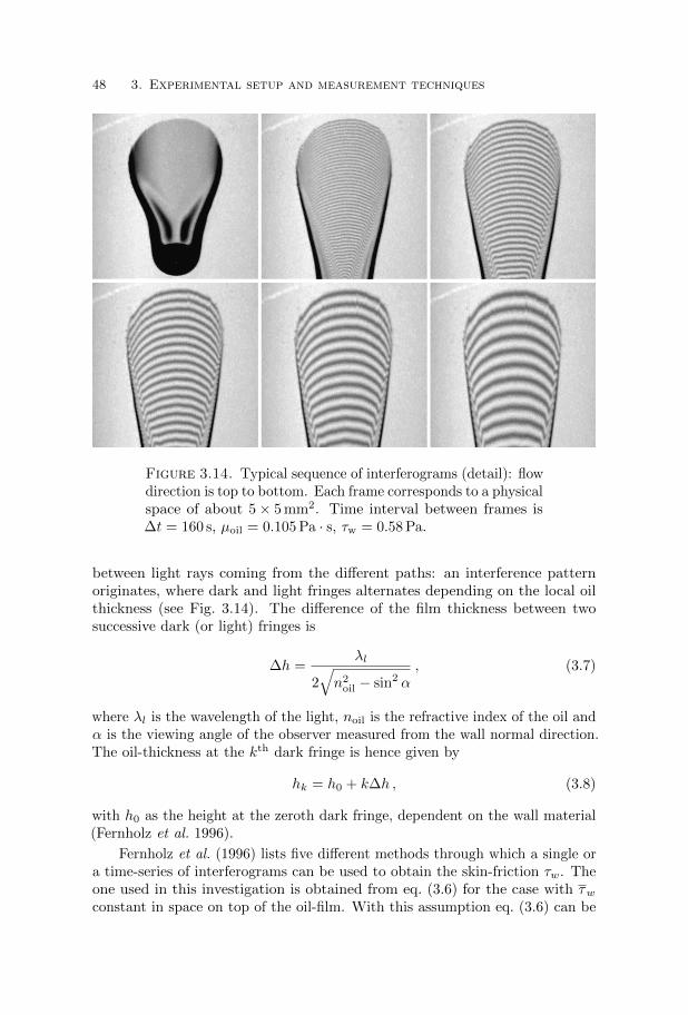
48 3. Experimental setup and measurement techniques
Figure 3.14. Typical sequence of interferograms (detail): flowdirection is top to bottom. Each frame corresponds to a physicalspace of about 5× 5 mm2. Time interval between frames is∆t = 160 s, µoil = 0.105 Pa · s, τw = 0.58 Pa.
between light rays coming from the different paths: an interference patternoriginates, where dark and light fringes alternates depending on the local oilthickness (see Fig. 3.14). The difference of the film thickness between twosuccessive dark (or light) fringes is
∆h =λl
2√n2oil − sin2 α
, (3.7)
where λl is the wavelength of the light, noil is the refractive index of the oil andα is the viewing angle of the observer measured from the wall normal direction.The oil-thickness at the kth dark fringe is hence given by
hk = h0 + k∆h , (3.8)
with h0 as the height at the zeroth dark fringe, dependent on the wall material(Fernholz et al. 1996).
Fernholz et al. (1996) lists five different methods through which a single ora time-series of interferograms can be used to obtain the skin-friction τw. Theone used in this investigation is obtained from eq. (3.6) for the case with τwconstant in space on top of the oil-film. With this assumption eq. (3.6) can be

3.7. Skin-friction measurement 49
rewritten in the form of an advection equation
∂h
∂t+τwh
µoil
∂h
∂x= 0 , (3.9)
which tells us that the kth dark fringe moves with speed
uk =τwhkµoil
. (3.10)
Combining eq. (3.10), (3.8), (3.7) the shear stress can finally be expressed as
τw
(k +
h0∆h
)= µoiluk
2√n2oil − sin2 α
λl. (3.11)
From a time-series of interferograms, it is possible to follow the movement ofmany fringes, hence many fringe speeds uk can be determined. For each fringe,eq. (3.11) can be written, hence an overdetermined system of linear equationscan be built with unknowns τw and h0/∆h. Solving this system the mean wallshear stress can be determined without any a priori knowledge of h0/∆h.
Oil-film interferometry setup and data processing
The oil-film interferometry measurements were conducted on a glass plug insertedin the plate element equipped with the wall-mounted traverse (see §3.2.2). Theplug is cylindrical with diameter 48 mm and is made of an inner glass cylindermounted inside an outer aluminum ring equipped with a pressure-tap. Theinner cylinder is made of N-BK7 borosilicate glass 40 mm in diameter and 4 mmthick. In order to measure the temperature of the surface during a run, athermocouple is pressed in contact to the bottom surface of the glass. The plugcan be accurately aligned with the surface of the plate with three set screws.A mistake in the design phase led to a streamwise misalignment between thelocation of the hot-wire probe and the oil-film interferometry plug. However,for the range of Rex considered (Rex ' 5 × 10⁶), the misalignment resultsin a variation of τw < 0.2%, smaller than the estimated uncertainty on theskin-friction determination via oil-film interferometry.
The light source is a sodium-vapour lamp (λl = 589 nm) and the interfer-ograms were recorded with a Nikon D7100 camera placed on the roof of thewind-tunnel with a 200 mm focal-length objective, resulting in a resolution of70 px/mm. The view-angle α of the camera was measured with a digital anglegauge with resolution ±0.1. The photos were taken at interval ranging from4 s to 15 s depending on the shear-stress level. The oil employed was silicone oilDOW CORNING 200 fluid, with a nominal kinematic viscosity of 100 mm2/s.The oil-viscosity variation with temperature has been measured with a Ubbelo-hde viscometer (accuracy ±0.1%) immersed in a temperature-controlled heatedbath and the results are shown in Figure 3.15. The viscometer provides ameasurement for the kinematic viscosity, from which the dynamic viscosity can

50 3. Experimental setup and measurement techniques
290 292 294 296 298 300 302 3040.085
0.09
0.095
0.1
0.105
0.11
0.115
T (K)
µoil (
Pa⋅
s)
Figure 3.15. Variation of the oil kinematic viscosity withtemperature. Solid line: Fit of eq. (3.13) through the measuredpoints.
be calculated
µoil(T ) = ρoil(T )νoil(T ) =ρoil(T0)
1 + C1(T − T0)νoil(T ) , (3.12)
where the values of the constants were provided by the manufacturer (ρ0 =964 kg/m3, T0 = 298.15 K, C1 = 0.96 × 10⁻³). To calculate the viscosity attemperatures other than the calibration points, the relation
µoil = C2 e C3/T (3.13)
was used3, with the value of the constants obtained from a fit through themeasured points (C2 = 218.4× 10⁻³ Pa·s ; C3 = 1819 K). The oil refractionindex has been obtained from the data provided by the manufacturer.
Before starting a measurement, the wind tunnel was run for a long time(more than one hour) so that all the components reached a steady temperature.Since the lower surface of the test plate is not immersed in the flow, but isfacing the laboratory, the temperature in the test section was set to be closeto room temperature (∆T < 1 C), in order to limit the heat transfer at theplug. The flow was then stopped and one or several drops of oil were quicklypositioned on the glass plug with the help of a needle. The wind tunnel wasturned on again and the acquisition of the images was started as soon as theair and the plug reached a steady temperature. The maximum temperaturevariation observed on the plug during a run was 0.1 K. The quality of the oilflow can be severely decreased by the presence of dust particles, and care mustbe taken to work in a clean environment and with clean tools. Cleaning the
3The relation is commonly known as Andreade equation, even if it was originally proposed byde Guzman (1913) (see Viswanath et al. 2007).

3.7. Skin-friction measurement 51
t (s)
x (
mm
)
200 400 600 800 1000
20
16
12
8
4
0
Figure 3.16. Typical x − t diagram obtained from a timeseries of interferograms. Red dashed lines : user-identified fringecentre.
glass plug and the needle before each run with a lens tissue wet in acetonehelped to reduce the number of runs largely affected by dust deposition.
From each series of interferograms several x−t diagrams can be constructed:one line of pixels parallel to the flow direction is selected and extracted fromall the interferograms. An x− t diagram is then obtained assembling all theextracted lines in a single figure as shown in Figure 3.16. The x− t diagramswere then analyzed with a semi-automatic computer program, originally writtenby Osterlund (1999) and further modified by Ruedi et al. (2003) and by thepresent author. The user is required to manually locate the fringe centre (peakof the greyscale intensity), an example is shown with the red dashed line inFigure 3.16. To improve accuracy, each measurement was repeated between 3to 5 times and from each of the runs, showing a large area not contaminatedby dust particle 3 different x− t diagrams were obtained and analyzed. Thereproducibility of the measured τw proved to be better than ±2%, in closeagreement with the accuracy estimate provided in Nagib et al. (2004) (±1.5%).
3.7.2. Hot-film sensors
During this investigation, an attempt to measure the wall shear stress in presenceof suction and blowing with hot-film sensors was conducted. Tao Systems SenflexSF0303 hot-films were glued on eight 10 mm diameter cylindrical plugs andaligned flush to the plate with the help of two set screws. Particular care was
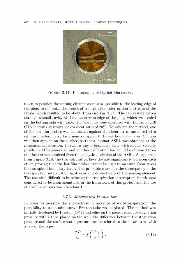
52 3. Experimental setup and measurement techniques
Figure 3.17. Photography of the hot film sensor.
taken to position the sensing element as close as possible to the leading edge ofthe plug, to minimize the length of transpiration interruption upstream of thesensor, which resulted to be about 3 mm (see Fig. 3.17). The cables were driventhrough a small cavity at the downstream edge of the plug, which was sealedon the bottom side with tape. The hot-films were operated with Dantec 90C10CTA modules at resistance overheat ratio of 20%. To validate the method, oneof the hot-film probes was calibrated against the shear stress measured withoil film interferometry for a non-transpired turbulent boundary layer. Suctionwas then applied on the surface, so that a laminar ASBL was obtained at themeasurement location. In such a way a boundary layer with known velocityprofile could be generated and another calibration law could be obtained fromthe shear stress obtained from the analytical solution of the ASBL. As apparentfrom Figure 3.18, the two calibration laws deviate significantly between eachother, proving that the hot-film probes cannot be used to measure shear stressfor transpired boundary-layer. The probable cause for the discrepancy is thetranspiration interruption upstream and downstream of the sensing element.The technical difficulties in reducing the transpiration interruption length wereconsidered to be insurmountable in the framework of this project and the useof hot-film sensors was abandoned.
3.7.3. Miniaturized Preston tube
In order to measure the shear-stress in presence of wall-transpiration, thepossibility to use a miniaturize Preston tube was explored. The method wasinitially developed by Preston (1954) and relies on the measurement of stagnationpressure with a tube placed on the wall: the difference between the stagnationpressure and the surface static pressure can be related to the shear stress witha law of the type
∆P
τw= f
(d2τwρν2
). (3.14)

3.7. Skin-friction measurement 53
2.26 2.28 2.3 2.32 2.34 2.36 2.380
0.5
1
1.5
2
2.5
3
E (V)
τw
(N
/m2)
+97%
laminar calib. (ASBL)
turbulent calib. (OFI)
Figure 3.18. Comparison between the hot-film calibrationlaw obtained in a non-transpired TBL and the one obtainedfor a laminar ASBL.
Preston tube method does not provide a direct measurement of the skin-friction,since the measured quantity is the mean velocity in the tube in disguise. However,the method proved to work as long as the tube is fully immersed in the regionwhere the law of the wall is valid. Preston tubes are typically calibrated in afully-developed pipe flow, where a direct measurement of the skin friction canbe obtained from the pressure-drop, with the Preston-tube diameter d+ lyingmainly in the logarithmic region of the turbulent boundary layer (see Patel 1965;Head & Vasanta Ram 1971; Bechert 1996). In presence of wall transpiration,however, the law of the wall for non-suction turbulent boundary layer does notrepresent accurately the mean velocity profile outside the viscous sublayer, asdepicted in Figure 3.19 where DNS results in the inner region of suction andimpermeable turbulent boundary layer are compared. Consequently, as longas the Preston tube lies outside of the viscous sublayer, a different calibrationlaw would apply for transpired or impermeable boundary layers, in analogy towhat occurs in pressure gradient boundary layers (Patel 1965; Hirt & Thomann1986). Simpson & Whitten (1968) proposed a calibration for Preston tubemeasurements in presence of wall transpiration, basing their conclusions on theSimpson’s law of the wall (Simpson 1967): as a consequence, this approach isbiased and cannot be used to validate a mean-velocity profile scaling. A differentPreston tube correction for wall transpiration was later proposed by Baker et al.(1971), a modified version of which was later recommended by Depooter et al.(1978), on the basis of shear-stress data measured with an ingeniously builtporous floating element.
If the tube opening resides fully in the viscous sublayer, a single calibrationcurve is expected to apply in all cases, independently of transpiration rate or

54 3. Experimental setup and measurement techniques
100
101
102
0
5
10
15
20
y+
U+
TASBL
ZPG TBL
Figure 3.19. Comparison between the mean velocity profileof a ZPG TBL (DNS data by Schlatter & Orlu 2010, forReθ = 4060) and a TASBL (DNS data by Khapko et al. 2016for Γ = 3.571× 10⁻³).
pressure gradients. For this reason an attempt to build a miniaturized Prestontube always lying entirely in the viscous sublayer was explored. The mainadvantage of the use of a Preston tube for our purpose is that the tube canbe placed directly on the transpired region, without the need to interrupt thesuction/blowing for a certain distance. Due to the large shear stress levelencountered in suction boundary layer, however, the size limitation on the tubediameter are stringent. In order to obtain an inner-scale diameter d+ < 3 in anasymptotic suction boundary layer with U∞ = 25 m/s and Γ = 3× 10⁻³ in airν = 1.55× 10⁻⁵, the diameter of the Preston tube must be
d < 3l∗ = 3ν
uτ= 3
ν
U∞√
Γ−1= 34 µm . (3.15)
Pipettes used for in-vitro fertilization have diameters ranging from 6 µm to 40 µmand are easily available, representing an appealing choice. Such a Preston tubecould be calibrated in a conventional ZPG TBL, and later used in transpiredboundary layer providing reliable results. As a verification an ASBL at moderatespeed could be used, for which an analytical expression for the shear-stressis available. To test this approach a Wallace ICSI WBB-30Z-30 polar biopsypipette with 32 µm external diameter, and 1 µm wall thickness was used (seeFig. 3.20 and Fig. 3.21 for a sketch of the geometry). The pipette was mountedin a support that could be inserted in the 10 mm plate access plug at the plateequipped with the oil-film interferometry plug. Accurate positioning of thepipette on the wall was obtained traversing the support in the plate-normaldirection with a micrometer screw while observing the position of the pipettetip with a microscope. The differential pressure between the stagnation and

3.7. Skin-friction measurement 55
Figure 3.20. Photography of the miniaturized Preston tube.In the inset a magnified view of the tip of the pipette is shown.
30°
56 - 60 mm Ø 32 μmØ 30 μm
Figure 3.21. Sketch of the Wallace ICSI WBB-30Z30 polarbiopsy pipette.
the static pressure measured at the wall (in a different spanwise position)was measured with a Furness FCO560 pressure calibrator with range 200 Pa.Due to the small tube opening, concerns on the frequency response of thepressure measurement raised. To estimate the time response of the system, thewind-tunnel was run for long times (hours) and then rapidly halted while theresponses of the Preston tube and of a Prandtl tube in the free stream weremonitored. The results are shown in Figure 3.22. It can be noticed that twohours after the flow was stopped, the stagnation pressure did not still reach thezero value. The time response of the miniaturized Preston tube appeared to

56 3. Experimental setup and measurement techniques
0 0.5 1 1.5 20
5
10
15
20
Pre
ston ∆
P (
Pa)
0 0.5 1 1.5 20
10
20
30
t (hours)
U∞
(m
/s)
Figure 3.22. Time response of the miniaturized Preston tube.
be insufficient for any practically interesting laboratory application. The causeof the slow response is probably the very small diameter and comparably longextent of the opening. In fact, if the tip of the pipette was cut such that theexternal diameter became ≈ 100 µm, the time response considerably improvedbut the size limitation of eq. (3.15) could not be met. Due to the insufficienttime response of the miniaturized Preston tube, the method was abandoned.

Chapter 4
Measurement procedure and data reduction
4.1. Preparation of an experiment
A typical experiment consisted in the acquisition of velocity time series forseveral boundary-layer profiles. As a first operation the extent of the walltranspiration was regulated either by disconnecting the upstream plate elementsfrom the suction/injection system or by covering a portion of the surface withstandard household aluminium foil, which was taped to the plate at its fouredges. The regulation of the transpiration region with aluminium foil could onlybe performed for the suction cases, since in presence of wall injection the foilwould detach from the surface. The desired suction/injection rate was obtainedby regulating the fan rotation speed, while the desired uniformity was achievedby adjusting eight valves on the suction chamber (one for each plate element).For all the measurements performed employing the supported traverse system,the zero-pressure-gradient condition was checked with streamwise traversesof the hot wire in the free stream. Readings from the pressure taps at theplate surface were instead used when the wall-mounted traverse was in useand the supported traverse unmounted. A rather tedious iterative regulationof the ceiling shape and/or of the bleed-slot opening allowed to establish azero-pressure-gradient free stream velocity distribution for all the experimentalconditions for 1.5 m / x / 6.5 m, as shown in Figure 4.1. Once the experimentalconditions were set, all the measured quantities were logged and the hot-wirescans of the velocity field were performed by a fully automatic computer program.A full recalibration of the hot-wire probe after the acquisition of a minimumof two and a maximum of five boundary-layer profiles was also automaticallyperformed.
4.2. Heat transfer to the wall and outliers rejection
It is well known that hot-wire measurement are affected by the proximity ofa solid wall, since additional heat transfer occurs between the heated plumeemanating from the wire and the colder surface. If the conventional hot-wire free-stream calibration is used, the additional heat transfer manifests asan unphysical increase of the measured velocity with decreasing wall-normaldistance. In order to identify the data points affected by wall-proximity effectsthe method proposed by Orlu et al. (2010) is followed. It relies on the observation
57

58 4. Measurement procedure and data reduction
0.97
0.98
0.99
1
1.01
1.02
1.03U
∞/〈U
∞〉
a)
0 1 2 3 4 5 60.97
0.98
0.99
1
1.01
1.02
1.03
x(m)
U∞/〈U
∞〉
b) V
0=0
V0<0
V0>0
Figure 4.1. Variation of the free-stream velocity with thestreamwise coordinate. 〈U∞〉 indicates the streamwise aver-aged value of the free-stream velocity. a) Hot-wire velocity-measurement in the free stream for all the experiments per-formed with the supported traverse system. b) Pressure-taps reading for all the experiments performed with the wall-mounted traverse system at x = 6.06 m. Dashed lines:〈U∞〉 ± 0.5%.
that the local turbulence intensity√u′2/U in the viscous sublayer increases
monotonically reaching its peak value at the wall (see Fig. 4.2). A decrease ofthe measured local turbulence intensity in proximity of the wall can hence beexplained by an additional heat transfer to the wall, responsible to an apparent
increase of U and/or a decrease of√u′2. In the current experiments all the
data points closer to the wall than the location of the measured peak of localturbulence intensity were considered to be outliers and rejected (see Fig. 4.4).

4.3. Estimation of friction velocity and absolute wall distance 59
0 10 20 300
0.1
0.2
0.3
0.4
0.5
0.6
y+
√
u′2 /U
TASBL V
0/U
∞ = −2.50 × 10
−3 [1]
TASBL V0/U
∞ = −3.00 × 10
−3 [1]
TASBL V0/U
∞ = −3.45 × 10
−3 [2]
TASBL V0/U
∞ = −3.57 × 10
−3 [2]
TASBL V0/U
∞ = −3.70 × 10
−3 [2]
ZPG TBL V0/U
∞ = 0, Re
θ=3626
[3]
Blowing TBL V0/U
∞ = +1.00 × 10
−3,
Reθ = 2395
[4]
Figure 4.2. Near-wall local turbulence-intensity distributionfor TASBLs, a non-transpired boundary layer and a blowingboundary layer. [1]: LES by Bobke et al. (2016); [2]: DNS by
Khapko et al. (2016); [3]: DNS by Schlatter & Orlu (2010); [4]:LES by Kametani et al. (2015).
4.3. Estimation of friction velocity and absolute wall distance
A good estimate of the friction velocity uτ and of the absolute wall positionis essential in the description of the flow, especially when viscous scaling isused as normalization. In some cases, namely non-transpired boundary layermeasured at the most downstream measurement station, a direct measurementof the wall shear stress with oil film interferometry was available, but forall the other remaining cases the wall shear stress needed to be estimatedindirectly. A direct measurement of the wall position with sufficient accuracywas unavailable in most of the cases: the rotary encoder of the traverse systemused can provide an accurate measurement of the relative displacement of thehot-wire probe but not of the absolute position of the probe in respect tothe wall. For measurements at the most downstream measurement station(x = 6.06 m, see §3.2.2), a measurement of the wall position was obtainedobserving the wire and the surface with a microscope mounting a micrometerfocus gauge. The estimated uncertainty is ±20 µm, which is insufficient formost of the non-transpired turbulent boundary layers (`∗ = 11 µm to 34 µm)and for all the turbulent suction boundary layer (`∗ ≈ 7.5 µm) measured at thatlocation. In the following paragraphs the procedure followed to determine uτand the absolute wall position is given for each type of experiments reported inthe results section.

60 4. Measurement procedure and data reduction
4.3.1. Non-transpired turbulent boundary layers
For cases measured at the most downstream measurement station, a directmeasurement of uτ was available through OFI (see §5.1.2 for details). Themeasured values of U+ could then be used to find the absolute wall normalposition applying a wall-normal shift to the viscous scaled velocity profile fittingit in a least-square sense to DNS data in the inner region. This procedurewas applied just to data-points with U+ < 10, corresponding to y+ / 13,
and the simulation data employed were the ones by Schlatter & Orlu (2010)at Reθ = 4060. The result of the procedure is illustrated in Figure 4.4. Forcases measured at streamwise positions different from x = 6.06 m, no directmeasurement of the wall shear stress was available: in these cases a least-squarefit extended up to y+ ≈ 35 to the aforementioned DNS data was performed todetermine both the y-shift and the friction velocity.
4.3.2. Laminar/transitional suction boundary layers
For the laminar ASBL profiles (see Fig. 5.12), the absolute wall position wasobtained applying a y-shift determined with a fit to the ASBL solution to themeasured y. The absolute wall positions determined for each profile agreebetween each other with a maximum deviation of ±5 µm around their meanvalue, which in turn deviates less than 20 µm from the microscope observationsof the wire distance from the wall. Since the fitting procedure acts as a rigidshift of the profile, it does not alter the shape of the profile. The agreementobserved in Figure 5.12 between the experimental profiles and the ASBL solutionshould therefore not be consider an artifact of the fitting procedure. For thetransitional profiles shown in Figure 5.13, the fitting procedure to the ASBLsolution could not be applied: the wall position was hence fixed to the meanvalue of the one determined for the laminar ASBL profiles, measured in thesame set of experiments.
4.3.3. Turbulent suction boundary layers
For turbulent suction boundary layers the wall shear stress was calculated usingthe von-Karman momentum integral equation modified for mass-transfer. Inabsence of pressure gradients and neglecting the streamwise variation of theReynolds normal stresses difference u′2 − v′2 the following relation holds(
uτU∞
)2
=Cf
2=
dθ
dx− V0U∞
. (4.1)
Once uτ is determined for each profile, the absolute wall position is determinedwith a fit to simulation data of TASBL in the near-wall region (U+ < 10.5,corresponding to y+ / 18). The law of the wall for suction boundary layersis in general a function both of the absolute wall-normal position y+ andof the suction velocity V +
0 . In the range of suction rates considered (Γ =2.5× 10⁻³ − 3.70× 10⁻³), however, no significant difference is observed up toy+ = 20 (see Fig. 4.3).
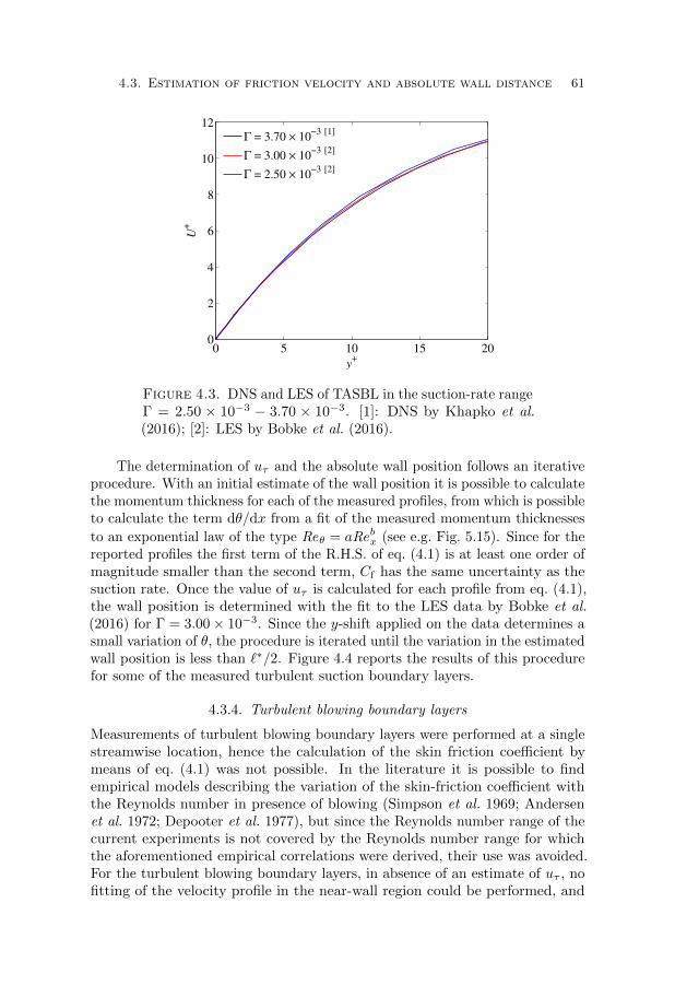
4.3. Estimation of friction velocity and absolute wall distance 61
0 5 10 15 200
2
4
6
8
10
12
y+
U+
Γ = 3.70 × 10⁻³
[1]
Γ = 3.00 × 10⁻³
[2]
Γ = 2.50 × 10⁻³
[2]
Figure 4.3. DNS and LES of TASBL in the suction-rate rangeΓ = 2.50 × 10⁻³ − 3.70 × 10⁻³. [1]: DNS by Khapko et al.(2016); [2]: LES by Bobke et al. (2016).
The determination of uτ and the absolute wall position follows an iterativeprocedure. With an initial estimate of the wall position it is possible to calculatethe momentum thickness for each of the measured profiles, from which is possibleto calculate the term dθ/dx from a fit of the measured momentum thicknesses
to an exponential law of the type Reθ = aRebx (see e.g. Fig. 5.15). Since for thereported profiles the first term of the R.H.S. of eq. (4.1) is at least one order ofmagnitude smaller than the second term, Cf has the same uncertainty as thesuction rate. Once the value of uτ is calculated for each profile from eq. (4.1),the wall position is determined with the fit to the LES data by Bobke et al.(2016) for Γ = 3.00× 10⁻³. Since the y-shift applied on the data determines asmall variation of θ, the procedure is iterated until the variation in the estimatedwall position is less than `∗/2. Figure 4.4 reports the results of this procedurefor some of the measured turbulent suction boundary layers.
4.3.4. Turbulent blowing boundary layers
Measurements of turbulent blowing boundary layers were performed at a singlestreamwise location, hence the calculation of the skin friction coefficient bymeans of eq. (4.1) was not possible. In the literature it is possible to findempirical models describing the variation of the skin-friction coefficient withthe Reynolds number in presence of blowing (Simpson et al. 1969; Andersenet al. 1972; Depooter et al. 1977), but since the Reynolds number range of thecurrent experiments is not covered by the Reynolds number range for whichthe aforementioned empirical correlations were derived, their use was avoided.For the turbulent blowing boundary layers, in absence of an estimate of uτ , nofitting of the velocity profile in the near-wall region could be performed, and
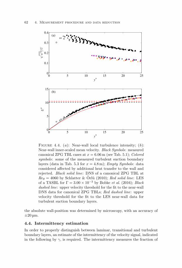
62 4. Measurement procedure and data reduction
0 5 10 15 20 250
5
10
15
y+
U+
(b)
0 5 10 15 20 250
0.1
0.2
0.3
0.4
y+
√
u′2 /U
(a)
Figure 4.4. (a): Near-wall local turbulence intensity; (b):Near-wall inner-scaled mean velocity. Black Symbols : measuredcanonical ZPG TBL cases at x = 6.06 m (see Tab. 5.1); Coloredsymbols: some of the measured turbulent suction boundarylayers (data in Tab. 5.3 for x = 4.8 m); Empty Symbols: dataconsidered affected by additional heat transfer to the wall andrejected. Black solid line: DNS of a canonical ZPG TBL atReθ = 4060 by Schlatter & Orlu (2010); Red solid line: LESof a TASBL for Γ = 3.00× 10⁻³ by Bobke et al. (2016); Blackdashed line: upper velocity threshold for the fit to the near-wallDNS data for canonical ZPG TBLs; Red dashed line: uppervelocity threshold for the fit to the LES near-wall data forturbulent suction boundary layers.
the absolute wall-position was determined by microscopy, with an accuracy of±20 µm.
4.4. Intermittency estimation
In order to properly distinguish between laminar, transitional and turbulentboundary layers, an estimate of the intermittency of the velocity signal, indicatedin the following by γ, is required. The intermittency measures the fraction of

4.4. Intermittency estimation 63
time in which the signal is in a turbulent state, taking the value γ = 0 whenthe signal is fully laminar and γ = 1 when the signal is fully turbulent. In orderto estimate the velocity-signal intermittency, the method proposed by Franssonet al. (2005) was used. It is an objective and user-independent method whichrequires as only parameter a cut-off frequency for a high-pass filter operationon the velocity signal. An accurate description of the procedure can be foundin Fransson et al. (2005).
In this work, the intermittency estimation procedure was applied to twodifferent cases: firstly it was used to determine the smallest suction rate for whichno turbulent spots are observed in an initially laminar boundary layer, secondlyit was used to determine at which suction rate an initially turbulent boundarylayer starts to show traces of relaminarization. In the first set of experiments,no tripping tape is used and suction is applied immediately downstream of theleading edge: in this configuration the boundary-layer profile evolves toward theASBL solution, with a characteristic length scale δ99,ASBL = ln(0.01)ν/V0. Thecut-off frequency was set to be U∞/(4δ99) (close to the value U∞/(5δ99) usedby Fransson et al. 2005). In the second set of experiments the boundary-layeris tripped at the leading-edge and the suction location is varied at differentdownstream location. The characteristic boundary-layer length scale can beapproximated with δ99,TASBL, which for the range of suction rate consideredcorresponds to roughly 10 to 20 times δ99,ASBL. The cut-off frequency was in thiscase chosen to be fcut = U∞/(4δ99,TASBL) approximated by U∞/(40δ99,ASBL).To verify that these choices of cut-off frequency are appropriate to obtain agood estimate of the intermittency of the velocity signal, the calculated valueγcalc are compared with the intermittency obtained from a visual inspectionof the velocity signal γvis. Figure 4.5 shows two different velocity signals, thetop one (a) was measured for an initially laminar boundary layer with tracesof turbulent spots, while the bottom one (b) was measured for an initiallyturbulent boundary layer undergoing relaminarization. The gray-shaded areasare the portion of the signal identified as turbulent by visual inspection. Forcase (a) γvisual = 0.22 and γcalc = 0.20, while for case (b) γvisual = 0.68 andγcalc = 0.79, demonstrating that the choices of fcut are appropriate.

64 4. Measurement procedure and data reduction
t (s)
U (
m/s
)
(a)
0 1 2 3 4 5 6 72
4
6
8
10
t (s)
U (
m/s
)
(b)
0 0.1 0.2 0.3 0.4 0.5 0.6 0.7
10
15
20
25
Figure 4.5. Velocity-signal for two transitional boundarylayers. (a): initially laminar boundary layer (γvisual = 0.22and γcalc = 0.20). (b): initially turbulent boundary layer(γvisual = 0.68 and γcalc = 0.79). Gray-filled areas: portion ofthe signal identified as turbulent by visual inspection.

Chapter 5
Results and discussion
5.1. Zero-pressure-gradient turbulent boundary layer
This section reports results obtained for zero-pressure-gradient turbulent bound-ary layers in absence of wall-transpiration: the purpose is not to offer additionaldata or new insight on zero-pressure-gradient turbulent boundary layers, a topicwhich has been the subject of a large number of dedicated studies, but ratherto test the capability of the current setup to reproduce this well-known flowcase. Benchmarking the measured non-transpired TBL against the canonicalZPG TBL is a first proof of the quality of the setup and of the experimentalprocedures. If successful, it is possible to conclude, for instance, that thethreshold on the variation of local free-stream velocity used to define the ex-perimental approximation of a zero pressure gradient is sufficiently low, thatthe history effects from the leading-edge pressure-distribution and from thetripping devices are small enough and finally that the perforated surface canindeed be considered hydraulically smooth. Hot-wire measurements were con-ducted for different free-stream velocities at different streamwise locations(0.55 m < x < 5.15 m) with the landing traverse system (see §3.1.2). Additionalmeasurements were also performed at the measurement station on the mostdownstream plate element (x = 6.06 m) using the wall-mounted traverse. Forthe measurement at x = 6.06 m the skin friction, could be directly measuredwith oil-film interferometry, allowing a more careful analysis of the velocityprofiles.
5.1.1. Assessment of the canonical state
A turbulent boundary layer is here defined to be canonical when it is completelydescribed by the governing parameters of the flow, which for ZPG TBLs arethe properly normalized wall-normal distance and the local Reynolds number.In other words with this definition the canonical state is achieved when thereal flow case studied can be considered representative of the ideal flow casethat we intended to study, despite all the experimental imperfections suchas wall roughness, three dimensionality, free-stream turbulence and historyeffects originating from the leading-edge pressure gradient and from turbulence-triggering devices. To assess the quality of the measured turbulent boundarylayer, the procedure delineated by Chauhan et al. (2009) was followed. There,
65

66 5. Results and discussion
100
101
102
103
104
0
5
10
15
20
25
30
y+
U+
Composite profileExp. Re
θ = 14740
Figure 5.1. Comparison of one of the ZPG TBL profile atx = 6.06 m with the composite profile by Chauhan et al. (2009).The fitted parameters were uτ , δ, Π.
a large experimental data-set of ZPG TBL was analyzed on the basis of ananalytic formulation of the mean-velocity profile as a composite profile of thetype (Coles 1956)
U+composite = U+
inner(y+) +
2Π
κW(yδ
). (5.1)
It was concluded that a boundary layer can be considered canonical1 if its shapefactor H12 and wake parameter Π differ less than a certain threshold from theshape factor H12,num and the wake parameter Πnum of the composite profile atthe same Reynolds number.
The shape factor for all the measured non-transpired cases is shown inFigure 5.2, and compared with the one obtained from the composite velocityprofile. The proposed threshold ±0.008 for the maximum deviation permissiblefor the profile to be considered in an equilibrium state is also reported withdashed lines. Figure 5.3 reports instead the experimentally determined wakeparameters, together with Πnum and the proposed threshold Πnum ± 0.05. Thewake parameters were determined from a fit of all the points with y+ > 50 andy < δ99 to the composite profile in Chauhan et al. (2009). It can be noticed thatthe majority of the measured profiles appear to respect the criteria proposedfor the wake parameter, with more frequent deviations for Reθ / 7500. The
1In Chauhan et al. (2009) a different terminology is used, indicating with equilibrium what
here we denote with canonical.

5.1. Zero-pressure-gradient turbulent boundary layer 67
5 10 15 201.25
1.3
1.35
1.4
1.45
1.5
Reθ × 10
−3
H1
2
Figure 5.2. Shape factor H12 against the momentum thick-ness Reynolds number Reθ for all the measured non-transpiredcases. Filled symbols: profiles at x = 6.06 m; Solid line:H12,num obtained from the integration of the composite profileproposed in Chauhan et al. (2009); Dashed line: H12,num±0.008;Dotted line: H12,num ± 1% .
shape-factor criteria appears to be more stringent than the wake-parametercriteria, with a larger number of profiles outside of the proposed bounds, againmainly for Reθ / 7500. These deviations at lower Reynolds number can be anindication of over or under tripping or of history effects originating from theleading-edge pressure gradient. For large enough Reynolds number, however,the measured profiles can be considered to be equilibrium ZPG TBL profiles,proving the quality of the present apparatus and of the experimental procedures.As additional proof, the next sections will report the measured skin-frictioncoefficient and the velocity profiles at the most downstream measurementlocation.
5.1.2. Skin-friction coefficient
Skin-friction measurements with oil-film interferometry were performed at themost downstream measurement station (xOFI = 6.13 m) for different free-streamvelocities. Each measurement was repeated from three to five times, and severalx − t diagrams (hence several value of τw) were obtained from each run (see§3.7.1). The mean value of the measured skin friction τw, was used to obtain

68 5. Results and discussion
5 10 15 200
0.1
0.2
0.3
0.4
0.5
0.6
0.7
0.8
Reθ × 10
−3
Π
Figure 5.3. Wake parameter Π against the momentum thick-ness Reynolds number Reθ for all the measured non-transpiredcases. Filled symbols: profiles at x = 6.06 m; Solid line: Πnum
for the composite profile proposed in Chauhan et al. (2009);Dashed line: Πnum ± 0.05 .
the skin-friction coefficient
Cf =τw
12ρU
2∞, (5.2)
with U∞ measured with a Prandtl tube located in the free stream above themeasurement location. The results are reported in Figure 5.4 together witha power-law fit through the data and the 1/7th power law with the modifiedcoefficient proposed in Nagib et al. (2007). The power-law fit was then usedto calculate the skin-friction coefficient, and hence the friction velocity uτ , fora series of velocity profiles measured with the wall-mounted traverse at thelocation x = 6.06 m. The skin-friction coefficients obtained with this procedureare plotted against the momentum-thickness Reynolds number in Figure 5.5 andcompared with the Coles-Fernholz skin friction law eq. (1.35) with parametersκ = 0.384 and C = 4.127 as proposed by Nagib et al. (2007). Good agreementbetween the OFI measurements and the Coles-Fernholz skin-friction law isfound, with larger deviation (even though limited to less than 2%) for the twosmallest Reynolds numbers considered.
5.1.3. Statistical quantities
Seven boundary-layer profiles were measured at the most downstream measure-ment location x = 6.06 m for different free-stream velocities, with the main

5.1. Zero-pressure-gradient turbulent boundary layer 69
4 6 8 10 12 14 16 18 202.1
2.2
2.3
2.4
2.5
2.6
2.7
Rex × 10
−6
Cf ×
10
3
C
f = 0.022 Re
x
−0.138
Cf = 0.024 Re
x
−1/7
Figure 5.4. Skin friction coefficient measured with oil-filminterferometry. The error bars show a ±2% variation in Cf .Solid line: power-law fit through the measured data; Dashedline: 1/7th law with coefficient proposed by Nagib et al. (2007).
experimental parameters listed in Table 5.1. For these profiles uτ was estimatedfrom the oil-film interferometry measurements. The mean-velocity profile ininner scaling is shown in Figure 5.6, together with the linear and logarithmiclaw of the wall
U+ = y+ (5.3)
and
U+ =1
κln y+ +B (5.4)
with constants κ = 0.384 and B = 4.173 as proposed by Nagib et al. (2007).Good overlap of the data in the inner region is observed for all the profilesconsidered, as expected from the classical turbulent-boundary-layer theory.Figure 5.7, shows the mean velocity defect scaled with the friction velocityU+∞ − U+ in outer scaling, with the Rotta-Clauser length scale ∆ = δ∗U∞/uτ
as the outer length scale. The good collapse of the data when looking at thevelocity defect in outer scaling gives additional confidence that the equilibriumstate was attained for the boundary-layer profiles considered. The dashed linein Figure 5.7 represents the log law expressed in the velocity-defect formulation
U+∞ − U+ = − 1
κln η +B1 , (5.5)
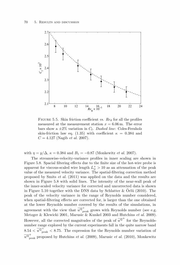
70 5. Results and discussion
8 10 12 14 16 18 20 22 242.1
2.2
2.3
2.4
2.5
2.6
2.7
Reθ × 10
−3
Cf ×
10
3
Figure 5.5. Skin friction coefficient vs. Reθ for all the profilesmeasured at the measurement station x = 6.06 m. The errorbars show a ±2% variation in Cf . Dashed line: Coles-Fernholzskin-friction law eq. (1.35) with coefficient κ = 0.384 andC = 4.127 (Nagib et al. 2007).
with η = y/∆, κ = 0.384 and B1 = −0.87 (Monkewitz et al. 2007).
The streamwise-velocity-variance profiles in inner scaling are shown inFigure 5.8. Spacial filtering effects due to the finite size of the hot-wire probe isapparent for viscous-scaled wire length L+
w > 10 as an attenuation of the peakvalue of the measured velocity variance. The spatial-filtering correction methodproposed by Smits et al. (2011) was applied on the data and the results areshown in Figure 5.8 with solid lines. The intensity of the near-wall peak ofthe inner-scaled velocity variance for corrected and uncorrected data is shownin Figure 5.10 together with the DNS data by Schlatter & Orlu (2010). Thepeak of the velocity variance in the range of Reynolds number considered,when spatial-filtering effects are corrected for, is larger than the one obtainedat the lower Reynolds number covered by the results of the simulations, in
agreement with the view that u′2+
peak grows with Reynolds number (see e.g.Metzger & Klewicki 2001, Marusic & Kunkel 2003 and Hutchins et al. 2009).
However, all the corrected magnitudes of the peak of u′2+
for the Reynolds-number range explored by the current experiments fall in the quite narrow band
8.54 < u′2+
peak < 8.75. The expression for the Reynolds number variation of
u′2+
peak proposed by Hutchins et al. (2009), Marusic et al. (2010), Monkewitz

5.1. Zero-pressure-gradient turbulent boundary layer 71
100
101
102
103
104
0
5
10
15
20
25
30
y+
U+
Figure 5.6. Inner-scaled mean-velocity profiles for x = 6.06 m.Dashed-dotted line: linear-law eq. (5.3); Dashed line: log-laweq. (5.4) with constants κ = 0.384 and B = 4.173 (Nagib et al.2007). Symbols as in Tab. 5.1.
10−3
10−2
10−1
100
0
5
10
15
20
25
y/∆
U∞+
−U
+
Figure 5.7. Outer-scaled velocity-defect profiles for x =6.06 m. Dashed line: log-law eq. (5.5) with constants κ = 0.384and B1 = −0.87 (Monkewitz et al. 2007). Symbols as inTab. 5.1.

72 5. Results and discussion
Table 5.1. Experimental parameters for the ZPG TBL profilesmeasured at x = 6.06 m.
Case
U∞ (m/s) 12.5 15.0 20.0 25.0 29.9 34.9 39.8uτ (m/s) 0.450 0.531 0.696 0.855 1.011 1.167 1.321Cf × 103 (-) 2.58 2.52 2.42 2.34 2.29 2.24 2.20`∗ (µm) 33.5 28.3 21.6 17.5 14.8 12.9 11.4θ (mm) 9.90 9.63 9.29 8.84 8.36 8.22 8.05δ∗ (mm) 13.42 13.00 12.37 11.68 10.99 10.78 10.50δ99 (mm) 83.74 84.99 81.87 78.29 77.99 77.88 76.42Reθ (-) 8230 9580 12360 14740 16650 19090 21330Reτ (-) 2500 3000 3790 4470 5250 6050 6710H12 (-) 1.36 1.35 1.33 1.32 1.31 1.31 1.30Π (-) 0.48 0.47 0.44 0.42 0.40 0.39 0.39Lw (mm) 0.280 0.280 0.280 0.280 0.280 0.280 0.280L+
w (-) 8.4 9.9 13.0 16.0 18.9 21.7 24.61/f+
max (-) 0.17 0.23 0.40 0.61 0.85 1.13 1.45tsmpU∞δ99
(-) 13500 15900 22000 25500 30700 31300 36500
& Nagib (2015), together with the constant value reported by Vallikivi et al.(2015) are shown in Figure 5.10 for a comparison with the present data.

5.1. Zero-pressure-gradient turbulent boundary layer 73
101
102
103
104
0
1
2
3
4
5
6
7
8
9
y+
u′2+
Figure 5.8. Symbols: measured inner-scaled streamwisevelocity-variance profiles for x = 6.06 m, symbols as in Tab. 5.1;Lines: data corrected for spatial-filtering effects with themethod by Smits et al. (2011).
0 0.05 0.1 0.15 0.2 0.25 0.3 0.350
0.002
0.004
0.006
0.008
0.01
0.012
y/∆
u′2/U
2 ∞
Figure 5.9. Outer-scaled streamise-velocity variance profilesfor x = 6.06 m. Symbols as in Tab. 5.1.

74 5. Results and discussion
Reτ
u′2+ p
eak
(a)
103
104
7
7.5
8
8.5
9
9.5
10
20 22 24 26 28 305
6
7
8
9
10
11
U +∞
u′2+ p
eak
(b)
u ′2+
peak= 4 .84 + 0 .47 lnRe[ 1]τ
u ′2+
peak= 4 .8 + 0 .38 lnRe[ 2]τ
u ′2+
peak= 2 .65 + 0 .69 lnRe[ 2]τ
u ′2+
peak= 8 .4 [ 3]
u ′2+
peak= 8 .4 [ 3]
u ′2+
peak= 22 − 340/U+ [4]∞
Figure 5.10. Variation of the near-wall peak of thestreamwise-velocity variance with the Reynolds number Reτ(a) and with U+
∞ (b). Filled symbols: current experiments(x = 6.06 m), data corrected with the method by Smits et al.(2011); Open symbols: current experiments, measured data;
Black crosses: DNS data by Schlatter & Orlu (2010); Lines:logarithmic trends proposed by [1] Hutchins et al. (2009) (ex-trapolated to L+
w = 0) and [2] Marusic et al. (2010), con-stant value proposed by [3] Vallikivi et al. (2015) for the range2600 < Reτ < 8300, expression proposed by [4] Monkewitz &Nagib (2015).

5.2. Zero-pressure-gradient suction boundary layers 75
5.2. Zero-pressure-gradient suction boundary layers
In this section the results obtained for boundary layer with wall-normal suctionare reported. Initially, laminar boundary layers are considered, with the inten-tion to verify that the apparatus is able to reproduce the laminar ASBL. Later,the range of suction rate for which turbulence can be maintained is investigatedand finally turbulent suction boundary layer are described, with the main focuson turbulent asymptotic suction boundary layers.
5.2.1. Laminar ASBL
A series of suction boundary-layer profiles were measured at the downstreammeasurement location x = 6.06 m for a free-stream velocity U∞ ≈ 10 m/s,with the suction applied immediately downstream of the leading-edge section(xs = 0.18 m) where no tripping tape was applied. In this configuration theFalkner-Skan boundary layer developing on the leading-edge section is expectedto evolve towards the ASBL velocity profile, which is obtained at a certaindownstream distance on the plate. Figure 5.11 shows the measured shape factorH12 corresponding to different suction rates Γ, together with the intermittencyvalue at y ≈ δ∗ calculated from the velocity-signal (see §4.4). The displacementthickness Reynolds number of the ASBL solution ReASBL (eq. 2.8) is alsoreported alongside the suction rate in the following figures, since it is the mostcommonly used parameter in the description of the flow. We observe that forall the profiles characterized by fully laminar velocity (γ = 0), the measuredshape factor coincide with the theoretical value H12 = 2. For this subset ofmeasurements the full velocity profile is illustrated in Figure 5.12 and comparedto the analytical ASBL solution. Excellent agreement is observed, proving thatan ASBL was indeed obtained at the measurement location for all the suctionrates Γ ≥ 3.38× 10⁻³ (ReASBL ≤ 296), providing a second proof of the qualityof the experimental apparatus and procedures. Figure 5.13 depicts the threeboundary-layers profiles for which an intermittent velocity was observed. Forthe profile at Γ = 2.92 × 10⁻³ (ReASBL = 343) the intermittency is still low(γ = 4% at y = δ∗) and the mean-velocity profile is still in good agreementwith the analytical ASBL solution. For increasing values of intermittency, themean-velocity profile departs from the ASBL solution, showing larger normalizedboundary-layer thickness and lower shape factor, related to the occurrence ofturbulent mixing in the boundary layer.
From the present data ona may conclude that in this particular setupintermittency in the velocity signal appears at a suction rate as high as Γ =2.92× 10⁻³ (ReASBL = 343). Care should be exercised in the generalization ofthese results. Since the critical Reynolds number according to linear stability istwo order of magnitude higher than the values of ReASBL for which turbulentprofiles were observed2, the transition of the ASBL is subcritical. The Reynolds
2Bussman & Muntz (1942) reported ReASBL,crit = 70 000 (see Schlichting & Gersten 2017,
§15.2.4c), Hocking (1975) reported ReASBL,crit = 47 000 and Fransson & Alfredsson (2003)
reported ReASBL,crit = 54 382.

76 5. Results and discussion
2 3 4 5 6 7 8 9 101.4
1.6
1.8
2
2.2
Γ × 103
H12
(a)
100200300400500
ReASBL
2 3 4 5 6 7 8 9 10
0
0.2
0.4
0.6
0.8
1
Γ × 103
γ (y
≈ δ
*)
(b)
100200300400500Re
ASBL
Figure 5.11. Boundary-layer shape factor H12 (a) andvelocity-signal intermittency γ (b) at x = 6.06 m for U∞ ≈10 m/s and xs = 0.18 m. In (a), Solid line: theoretical value ofshape factor for an ASBL (H12 = 2); Dashed lines: H12 =2± 1%.
number at which transition is observed depends on the perturbation level towhich the boundary layer is exposed (surface roughness, free-stream turbulenceintensity, leading-edge pressure gradients, smoothness at the plate joints etc.)and the extent of the streamwise distance along which the disturbances areallowed to grow. It is hence likely that a fully laminar ASBL exists for Γ <2.92× 10⁻³ (ReASBL > 343) under different conditions, as reported by Fransson(2010), where ASBL profiles at Re as high as ReASBL = 600 where obtained ina different experimental setup.
5.2.2. Self-sustained turbulence suction-rate threshold
Before discussing the turbulent state of suction boundary layer, it is crucial todefine the range of suction rate for which a turbulent state is self sustained. Itis known since the earliest studies on suction boundary layers that an initiallyturbulent boundary layer would relaminarize for large enough suction rates.

5.2. Zero-pressure-gradient suction boundary layers 77
0 0.2 0.4 0.6 0.8 10
1
2
3
4
5
6
7
8
9
10
U/U∞
−y V
0/ν
Γ = 9.41 × 10⁻³
Γ = 8.40 × 10⁻³
Γ = 7.51 × 10⁻³
Γ = 6.62 × 10⁻³
Γ = 4.78 × 10⁻³
Γ = 3.84 × 10⁻³
Γ = 3.61 × 10⁻³
Γ = 3.38 × 10⁻³
Figure 5.12. Velocity profiles for fully laminar boundarylayers at x = 6.06 m. Solid line: ASBL analytical velocityprofile.
0 0.2 0.4 0.6 0.8 10
5
10
15
20
25
U/U∞
−y V
0/ν
γ
0.2
0.4
0.6
0.8
1
Γ = 2.92 × 10⁻³
Γ = 2.47 × 10⁻³
Γ = 1.94 × 10⁻³
Figure 5.13. Velocity profiles for transitional boundary layersat x = 6.06 m. Solid line: ASBL analytical velocity profile.

78 5. Results and discussion
3.2 3.3 3.4 3.5 3.6 3.7 3.8 3.9 4 4.1 4.2
0
0.2
0.4
0.6
0.8
1
Γ × 10−3
γ
Rex,s
= 0.34 × 10⁶; ∆x/δ
s ≈ 950
Rex,s
= 0.52 × 10⁶; ∆x/δ
s ≈ 1030
Rex,s
= 1.99 × 10⁶; ∆x/δ
s ≈ 300
Rex,s
= 0.34 × 10⁶; ∆x/δ
s ≈ 680
Rex,s
= 1.67 × 10⁶; ∆x/δ
s ≈ 200
Rex,s
= 0.52 × 10⁶; ∆x/δ
s ≈ 740
Rex,s
= 2.02 × 10⁶; ∆x/δ
s ≈ 210
(a)
(b)
0 0.1 0.2 0.3 0.44
6
8
10
12
14
16
t (s)
U (
m/s
)
(a)
0 0.1 0.2 0.3 0.410
15
20
t (s)
U (
m/s
)
(b)
Figure 5.14. Top: Intermittency factor γ of the near-wallvelocity signal vs. the suction rate Γ for different suction startlocations Rexs and streamwise evolution lengths ∆x/δs. Blacksolid line: Γsst = 3.70 × 10⁻³ (Khapko et al. 2016); Blackdashed line: Γsst = 3.70× 10⁻³ ± 4%; Red dashed-dotted line:Γsst = 3.6 × 10⁻³ (Watts 1972). Bottom: Time series of thevelocity signal for the two sample cases indicated with (a) and(b).

5.2. Zero-pressure-gradient suction boundary layers 79
However, there are considerable differences in the literature regarding the valuesof the threshold suction rate Γsst (see §2.2.3). While the determination of Γsst isinteresting per se, its value is also important to avoid the inclusion of undesireddata in the analysis of turbulent suction boundary layers, since relaminarizingprofiles can carry misleading information in the study of the scaling of turbulentsuction boundary layers.
To obtain a measure of Γsst, experiments were conducted in which suctionwas applied starting from the normalized streamwise location Rex,s downstreamof an impermeable entry length on which a turbulent boundary layer developed(boundary-layer tripping is applied on the leading-edge section). At a down-stream distance ∆x from the commencement of suction, the velocity signal ismeasured in the inner region of the boundary layer (9 / y+ / 15) and theintermittency is calculated to determine whether the signal is fully turbulent,relaminarizing or fully laminar. The measurement is repeated for differentvalues of Γ and Rex,s and the results are shown in Figure 5.2.2. We observethat for all the initial conditions and evolution length considered the measuredself-substained turbulence suction-rate threshold fall in a ±4% bound from thevalue Γsst = 3.70× 10⁻³ reported by Khapko et al. (2016).
5.2.3. Development of turbulent boundary layer with suction
Turbulent suction boundary layers are expected to evolve towards an asymp-totic condition, for which the boundary layer becomes independent from thestreamwise coordinate. Earlier works suggested that to experimentally obtainan asymptotic turbulent state is difficult (or even impossible, Bobke et al. 2016),mainly because the evolution towards the asymptotic state is slow, i.e. occurringover a streamwise distance many times larger than the initial boundary layerthickness. The evolution to the asymptotic state can however be hastened ifthe boundary layer thickness at the location of the suction start is chosen to beclose to the asymptotic one (Dutton 1958; Black & Sarnecki 1958; Tennekes1964).
In order to test whether an asymptotic state could be obtained in thecurrent setup, a series of experiments where conducted in which the suctionrate was kept constant while the streamwise Reynolds number of the suction-start location Rex,s was gradually varied with a regulation of the free-streamspeed and of the physical suction-start location. The latter regulation wasobtained either disconnecting the upstream plate elements from the suctionsystem or, when finer adjustment was needed, covering a portion of the surfacewith standard households aluminium foil. The results for different suction ratesare shown in Figures 5.15 to 5.17, while in Table 5.2 the main experimentalparameters are listed. In Figures 5.15 to 5.17 x′ = x − xvo represent thestreamwise coordinate corrected for the virtual origin xvo calculated from thedownstream development of the canonical ZPG TBL cases. For all the suctionrates considered here, it was possible to experimentally realize a boundary layerwith approximately constant boundary-layer thickness, moreover for 4 out of 5
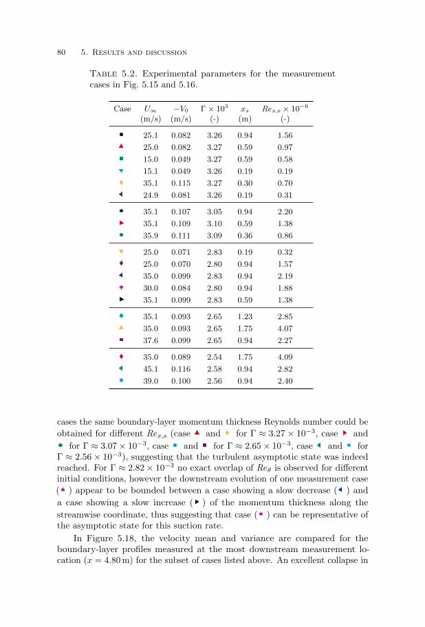
80 5. Results and discussion
Table 5.2. Experimental parameters for the measurementcases in Fig. 5.15 and 5.16.
Case U∞ −V0 Γ× 103 xs Rex,s × 10−6
(m/s) (m/s) (-) (m) (-)
25.1 0.082 3.26 0.94 1.56
25.0 0.082 3.27 0.59 0.97
15.0 0.049 3.27 0.59 0.58
15.1 0.049 3.26 0.19 0.19
35.1 0.115 3.27 0.30 0.70
24.9 0.081 3.26 0.19 0.31
35.1 0.107 3.05 0.94 2.20
35.1 0.109 3.10 0.59 1.38
35.9 0.111 3.09 0.36 0.86
25.0 0.071 2.83 0.19 0.32
25.0 0.070 2.80 0.94 1.57
35.0 0.099 2.83 0.94 2.19
30.0 0.084 2.80 0.94 1.88
35.1 0.099 2.83 0.59 1.38
35.1 0.093 2.65 1.23 2.85
35.0 0.093 2.65 1.75 4.07
37.6 0.099 2.65 0.94 2.27
35.0 0.089 2.54 1.75 4.09
45.1 0.116 2.58 0.94 2.82
39.0 0.100 2.56 0.94 2.40
cases the same boundary-layer momentum thickness Reynolds number could be
obtained for different Rex,s (case and for Γ ≈ 3.27× 10⁻³, case and
for Γ ≈ 3.07× 10⁻³, case and for Γ ≈ 2.65× 10⁻³, case and forΓ ≈ 2.56× 10⁻³), suggesting that the turbulent asymptotic state was indeedreached. For Γ ≈ 2.82× 10⁻³ no exact overlap of Reθ is observed for differentinitial conditions, however the downstream evolution of one measurement case
( ) appear to be bounded between a case showing a slow decrease ( ) and
a case showing a slow increase ( ) of the momentum thickness along the
streamwise coordinate, thus suggesting that case ( ) can be representative ofthe asymptotic state for this suction rate.
In Figure 5.18, the velocity mean and variance are compared for theboundary-layer profiles measured at the most downstream measurement lo-cation (x = 4.80 m) for the subset of cases listed above. An excellent collapse in
5.2. Zero-pressure-gradient suction boundary layers 81
the mean velocity profiles between the cases with matching suction rate is ob-served. The variance profiles for all the suction rates excluding Γ = 2.82× 10⁻³
also show excellent collapse in the outer region of the boundary layer, while theobservable deviation in the inner region can be explained by hot-wire spatialfiltering effects. For Γ = 2.82×10⁻³ the velocity variance profile show small butobservable differences in the outer region of the boundary layer, with the case
( ) having variance values between the ones of case ( ) and of case ( ). It is
concluded that all the cases reported in Figure 5.18 excluding ( ) and ( ) canbe considered turbulent asymptotic states. Figure 5.19 and 5.20 respectivelyshow the mean and variance velocity profiles at the three most downstreammeasurement locations for some of the cases identified as asymptotic. In thestreamwise-coordinate interval considered, corresponding to a streamwise dis-tance ∆x exceeding 20 times the boundary layer thickness δ99, the variation ofmomentum thickness is less than ±1.5% for all the cases considered. The varia-tion considering the full mean-velocity profiles is minimal and good overlap inthe outer part of the velocity variance profile is also observed. For completenessthe full evolution from a canonical ZPG TBL to the TASBL is illustrated inFigure 5.21 for case ( ). As expected the inner region adapt to the suction in ashort downstream distance, while a longer distance is required for the outer partof the boundary layer to reach the asymptotic condition. This is particularlyevident in the velocity variance profiles.
Concluding, for all the suction rates considered, it was possible to obtaina turbulent asymptotic state towards the downstream end of the flat plate:this was assessed observing that Reθ reached a constant value and that themean velocity and the outer part of the velocity variance profiles becameinvariant along the streamwise direction. For four out of the five suction ratesconsidered, the asymptotic Reθ and the asymptotic mean and variance velocityprofile could be obtained with two different initial conditions at the suctionstart, additional proof that the asymptotic state was indeed reached in a strictmanner. For one suction rate (Γ ≈ 2.82 × 10⁻³) the asymptotic value ofReθ and the velocity-variance profile could not be exactly reproduced withdifferent initial conditions, however Reθ and the velocity-variance profile appearto be bounded from two measurement cases with respectively slightly higherand lower streamwise coordinate Reynolds number at the suction start Rex,s .Table 5.3 summarizes the experimental conditions for which the asymptotic statecould be obtained and the boundary-layer parameters at the most downstreammeasurement station (x = 4.80 m). In Figure 5.22 the change in momentum-thickness Reynolds number and shape factor with the suction rate for theasymptotic states in Table 5.3 are plotted and compared with the simulationsresults by Bobke et al. (2016) and Khapko et al. (2016).
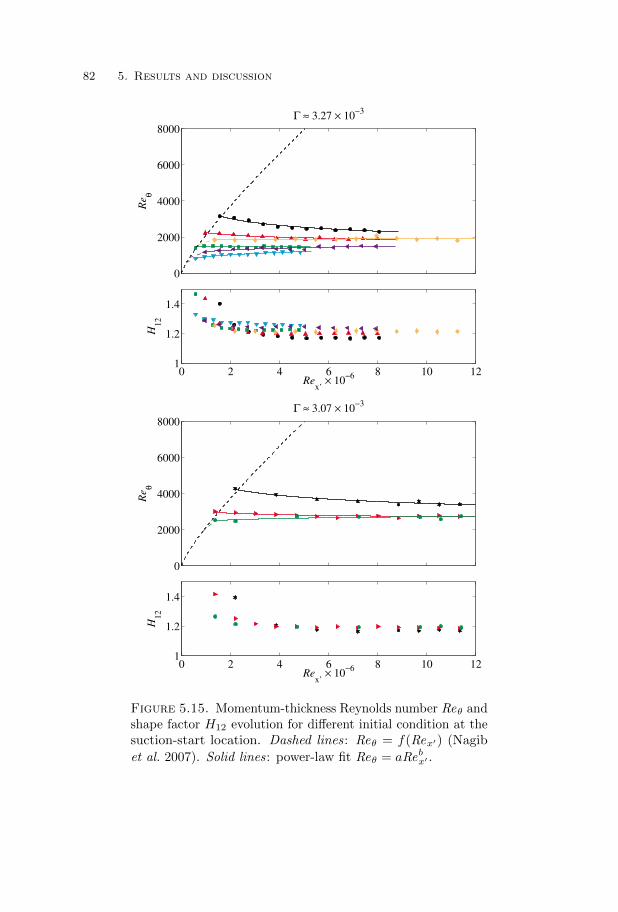
82 5. Results and discussion
0
2000
4000
6000
8000
Γ ≈ 3.27 × 10⁻³
Re
θ
0 2 4 6 8 10 121
1.2
1.4
Rex’
× 10−6
H12
0
2000
4000
6000
8000
Γ ≈ 3.07 × 10⁻³
Re
θ
0 2 4 6 8 10 121
1.2
1.4
Rex’
× 10−6
H12
Figure 5.15. Momentum-thickness Reynolds number Reθ andshape factor H12 evolution for different initial condition at thesuction-start location. Dashed lines: Reθ = f(Rex′) (Nagib
et al. 2007). Solid lines: power-law fit Reθ = aRebx′ .

5.2. Zero-pressure-gradient suction boundary layers 83
0
2000
4000
6000
8000
Γ ≈ 2.82 × 10⁻³
Re
θ
0 2 4 6 8 10 121
1.2
1.4
Rex’
× 10−6
H12
0
2000
4000
6000
8000
Γ ≈ 2.65 × 10⁻³
Re
θ
0 2 4 6 8 10 12 141
1.2
1.4
Rex’
× 10−6
H12
Figure 5.16. Momentum-thickness Reynolds number Reθ andshape factor H12 evolution for different initial condition at thesuction-start location. Dashed lines: Reθ = f(Rex′) (Nagib
et al. 2007). Solid lines: power-law fit Reθ = aRebx′ .

84 5. Results and discussion
0
2000
4000
6000
8000
Γ ≈ 2.56 × 10⁻³
Re
θ
0 2 4 6 8 10 12 141
1.2
1.4
Rex’
× 10−6
H12
Figure 5.17. Momentum-thickness Reynolds number Reθ andshape factor H12 evolution for different initial condition at thesuction-start location. Dashed lines: Reθ = f(Rex′) (Nagib
et al. 2007). Solid lines: power-law fit Reθ = aRebx′ .

5.2. Zero-pressure-gradient suction boundary layers 85
0
5
10
15
20
25
U+;10×
u′2+
Γ ≈ 3.27 × 10⁻³
L+
w ≈ 52
L+
w ≈ 80
0
5
10
15
20
25Γ ≈ 3.07 × 10
−3
L+
w ≈ 78
L+
w ≈ 79
0
5
10
15
20
25
U+;10×
u′2+
Γ ≈ 2.82 × 10⁻³
L+
w ≈ 75
L+
w ≈ 76
L+
w ≈ 64
100
101
102
103
104
0
5
10
15
20
25
y+
Γ ≈ 2.65 × 10⁻³
L+
w ≈ 72
L+
w ≈ 75
100
101
102
103
104
0
5
10
15
20
25
U+;10×
u′2+
y+
Γ ≈ 2.56 × 10⁻³
L+
w ≈ 79
L+
w ≈ 92
Figure 5.18. Inner-scaled velocity mean and variance profilesat x = 4.80 m. Dashed lines: Viscous sublayer. Colors andsymbols as in Tab. 5.2.

86 5. Results and discussion
0
5
10
15
20
U+
Γ = 3.27 × 10⁻³
∆x = 57 δ99
Rex = 9.60 × 10
6
Rex = 10.42 × 10
6
Rex = 11.25 × 10
6
0
5
10
15
20Γ = 3.10 × 10
−3
∆x = 37 δ99
Rex = 9.67 × 10
6
Rex = 10.50 × 10
6
Rex = 11.33 × 10
6
0
5
10
15
20
U+
Γ = 2.80 × 10⁻³
∆x = 24 δ99
Rex = 8.27 × 10
6
Rex = 8.98 × 10
6
Rex = 9.69 × 10
6
100
101
102
103
104
0
5
10
15
20
y+
Γ = 2.65 × 10⁻³
∆x = 20 δ99
Rex = 9.58 × 10
6
Rex = 10.40 × 10
6
Rex = 11.22 × 10
6
100
101
102
103
104
0
5
10
15
20
y+
U+
Γ = 2.58 × 10⁻³
∆x = 24 δ99
Rex = 12.42 × 10
6
Rex = 13.48 × 10
6
Rex = 14.55 × 10
6
Figure 5.19. Inner-scaled mean-velocity profiles for someasymptotic cases at the three most downstream measurementlocations. ∆x represents the streamwise distance betweenthe most upstream and the most downstream boundary-layerprofile shown in each graph. Colors as in Fig. 5.18. Dashedlines: Viscous sublayer.

5.2. Zero-pressure-gradient suction boundary layers 87
0
0.5
1
1.5
2
2.5
u′2+
Γ = 3.27 × 10⁻³
Re
x = 9.60 × 10
6
Rex = 10.42 × 10
6
Rex = 11.25 × 10
6
0
0.5
1
1.5
2
2.5
Γ = 3.10 × 10⁻³
Re
x = 9.67 × 10
6
Rex = 10.50 × 10
6
Rex = 11.33 × 10
6
0
0.5
1
1.5
2
2.5
u′2+
Γ = 2.80 × 10⁻³
Re
x = 8.27 × 10
6
Rex = 8.98 × 10
6
Rex = 9.69 × 10
6
101
102
103
104
0
0.5
1
1.5
2
2.5
y+
Γ = 2.65 × 10⁻³
Re
x = 9.58 × 10
6
Rex = 10.40 × 10
6
Rex = 11.22 × 10
6
101
102
103
104
0
0.5
1
1.5
2
2.5
y+
u′2+
Γ = 2.58 × 10⁻³
Re
x = 12.42 × 10
6
Rex = 13.48 × 10
6
Rex = 14.55 × 10
6
Figure 5.20. Inner-scaled velocity-variance profiles for someasymptotic cases at the three most downstream measurementlocations. Colors as in Fig. 5.18.

88 5. Results and discussion
100
101
102
103
104
0
5
10
15
20
25
30
y+
U+;5×
u′2+
Re
x = 0.95 × 10
6
Rex = 1.54 × 10
6
Rex = 2.71 × 10
6
Rex = 3.88 × 10
6
Rex = 5.05 × 10
6
Rex = 6.22 × 10
6
Rex = 7.39 × 10
6
Rex = 7.98 × 10
6
Figure 5.21. Evolution of the velocity mean and varianceprofiles from a ZPG TBL (Rex = 1.35× 10⁶) to a TASBL forΓ = 3.10× 10⁻³ and Rex,s = 1.38× 10⁶.

5.2. Zero-pressure-gradient suction boundary layers 89
2.4 2.6 2.8 3 3.2 3.4 3.60
2000
4000
6000
8000
Γ × 103
Re
θ, as
2.4 2.6 2.8 3 3.2 3.4 3.61
1.1
1.2
1.3
1.4
Γ × 103
H12, as
Figure 5.22. Momentum thickness Reynolds number Reθ andshape factor H12 variation with the suction rate. Filled symbols :asymptotic cases in Tab. 5.3; Open Blue Squares: LES databy Bobke et al. (2016); Open Red Diamonds: DNS data byKhapko et al. (2016).
5.2.4. Mean-velocity scaling for the turbulent asymptotic state
Once a series of TASBL profiles is identified, the problem of the appropriatemean-velocity scaling can be addressed. Figure 5.23 show the viscous-scaledmean-velocity profile for some of the measured TASBLs. The profiles appear tobe characterized by a large logarithmic region and by the absence of a clear wakeregion. The disappearance of the wake region was already reported in previousstudies and appears to be such a fundamental characteristics of TASBLs thatthe presence of a wake region can be considered a symptom that the boundarylayer has still not reached its asymptotic state (Black & Sarnecki 1958; Simpson1970; Bobke et al. 2016). These observations suggest that the logarithmic law
U+ = A(Γ) ln y+ +B(Γ) (5.6)
is a valid choice as an empirical description of the mean-velocity profile. However,a fairly large database of TASBLs at different suction rates is necessary todetermine the functions A = f1(Γ) and B = f2(Γ), while the amount of

90 5. Results and discussion
Table 5.3. Experimental parameters for all the measurementcases for which a TASBL was obtained and boundary-layerparameters for the profile at x = 4.80 m.
Case
U∞ (m/s) 25.0 35.1 35.1 35.9 30.0 35.1 37.6 39.0 45.1−V0 (m/s) 0.082 0.115 0.109 0.111 0.084 0.093 0.099 0.100 0.116Γ× 103 (-) 3.27 3.27 3.10 3.09 2.80 2.65 2.65 2.56 2.58xs (m) 0.59 0.30 0.59 0.36 0.94 1.23 0.94 0.94 0.94Rex,s × 10−6 (-) 0.97 0.70 1.38 0.86 1.88 2.85 2.27 2.40 2.82
x=
4.80
m
uτ (m/s) 1.43 2.01 1.95 2.00 1.58 1.81 1.94 2.00 2.30Cf × 103 (-) 6.48 6.51 6.17 6.19 5.61 5.30 5.29 5.20 5.19`∗ (µm) 10.6 7.5 7.7 7.6 9.4 8.4 8.0 7.6 6.5θ (mm) 1.16 0.77 1.16 1.16 1.86 2.22 2.07 2.18 1.86δ∗ (mm) 1.39 0.94 1.38 1.38 2.20 2.60 2.43 2.57 2.19δ99 (mm) 20.47 12.40 19.24 18.86 29.35 35.70 33.61 36.00 29.31Reθ (-) 1920 1800 2730 2740 3740 5170 5030 5600 5620Reτ (-) 1930 1660 2510 2480 3120 4270 4220 4720 4510H12 (-) 1.20 1.21 1.18 1.19 1.18 1.17 1.17 1.18 1.18Lw (mm) 0.55 0.60 0.60 0.60 0.60 0.60 0.60 0.60 0.60L+w (-) 52 80 78 79 64 72 75 79 92
1/f+max (-) 4.5 8.9 8.5 8.8 5.6 7.2 8.1 13.1 11.8tsmpU∞δ99
(-) 73500 125000 72900 66700 50900 44200 39400 38100 53900
experimental or numerical data available is indeed limited. In the followinganother approach is attempted: observing the mean-velocity profiles for the sameboundary layers plotted in outer scaling (see Fig. 5.24), a good overlap in theinner region can be noticed between all the TASBLs considered, independentlyfrom the suction rate. It follows that, at least in the range of suction rateconsidered, the TABLs profile can be described with the logarithmic law
U/U∞ = Ao ln η +Bo (5.7)
with the slope Ao and the intercept Bo constant for any suction rate. Regardingthe choice of the outer length-scale, three different choices (δ99, δ∗ and θ)are compared in Figure 5.24. No substantial difference between them can beobserved.
To further verify the mean-velocity scaling proposed in eq. (5.7), the indi-cator function
Ξ = yd(U/U∞)
dy(5.8)
was calculated for all the TASBLs listed in Table 5.2. Since the data were sam-pled nonequidistantly (namely with a logarithmic spacing) along the wall-normalcoordinate, the derivative was calculated with a weighted central-differencescheme of the type
dU
dy
∣∣∣∣y=yi
=
j=i+2∑j=i−2
wjUj (5.9)

5.2. Zero-pressure-gradient suction boundary layers 91
100
101
102
103
104
0
2
4
6
8
10
12
14
16
18
20
y+
U+
Γ=3.27 × 10⁻³
Γ=3.10 × 10⁻³
Γ=2.80 × 10⁻³
Γ=2.65 × 10⁻³
Γ=2.58 × 10⁻³
Figure 5.23. Viscous-scaled mean-velocity profiles of someof the measured TASBLs at x = 4.80 m. Dashed line: Viscoussublayer for Γ = 2.80× 10⁻³. Symbols as in Tab. 5.3.
with the weights wj calculated from the values of yi=j−2 , ... , j+2 following theprocedure proposed by Fornberg (1998) in order to maximize the accuracyat y = yi. The results are illustrated in Figure 5.25. A clear plateau of theindicator function is observed for y+ ' 150 and y/δ99 / 0.5 (corresponding toy ≈ δ95), indicating that the mean-velocity profile show indeed a logarithmicbehaviour along the wall-normal coordinate. The extent of this logarithmicregion is particularly large, extending for more than 40% of the boundary-layerthickness already for the lowest Reynolds (largest suction rate) considered(Reτ = 1760).
The slope Ao of the logarithmic region has been calculated for all theTASBLs profiles in Table 5.2 as the mean value of the indicator function fory+ > 150 and y/δ99 < 0.5. The results are shown in Figure 5.27: no clear trendof the value of the slope with the suction ratio can be distinguished and for allthe TASBLs profile considered Ao = 0.064± 5%. With this choice for Ao, theintercept Bo of the log-law can be calculated for each profile as the mean valuefor y+ > 150 and y/δ99 < 0.5 of
Ψ = U/U∞ −Ao ln η . (5.10)
For the choice of outer scale η = y/δ99 and Ao = 0.064, Figure 5.26 illustrates thefunction Ψ in inner- and outer-scaled wall-normal coordinate, while Figure 5.28reports the calculated value for Bo. The averaged value of the intercept Bo

92 5. Results and discussion
10−2
10−1
100
101
0.4
0.5
0.6
0.7
0.8
0.9
1
η=y/δ 99
η=y/(4θ)
η=y/δ*
η
U/U
∞
Γ=3.27 × 10⁻³
Γ=3.10 × 10⁻³
Γ=2.80 × 10⁻³
Γ=2.65 × 10⁻³
Γ=2.58 × 10⁻³
Figure 5.24. Outer-scaled mean-velocity profiles of some ofthe measured TASBLs at x = 4.80 m, for three different choicesof the outer length scale. The multiplicative coefficients ofthe length scales were chosen solely for illustration purposes.Dashed line: eq. (5.7) with Ao = 0.064 and Bo = 0.994. Sym-bols as in Tab. 5.3.
between all the profiles was found to be Bo = 0.994, 0.826 and 0.815 forη = δ99, δ
∗ and θ respectively.
From this analysis is also possible to derive an expression for A(Γ) andB(Γ) of eq. (5.6). We can rewrite eq. (5.7) as
U+ = U+∞(Ao ln η +Bo) , (5.11)
hence, choosing η = δ99
U+ = U+∞(Ao ln y+ −Ao ln Reτ +Bo,δ99) . (5.12)
Since for a TASBL U+∞ = 1/
√Γ, comparing eq. (5.6) and eq. (5.12)
A =Ao√
ΓB =
Bo,δ99 −Ao ln Reτ (Γ)√Γ
. (5.13)
Non-asymptotic turbulent suction boundary layers and mean-velocity scaling
Figure 5.29 and 5.30 illustrates, respectively in inner and outer scaling, twonon-asymptotic states at Γ ≈ 3.27× 10⁻³ together with the asymptotic stateat the same suction rate. In the two non asymptotic cases the presence of asmall but distinguishable wake region, compromises the validity of the proposed

5.2. Zero-pressure-gradient suction boundary layers 93
102
103
104
0
0.05
0.1
0.15
0.2
0.25
y+
Ξ
10−2
10−1
100
0
0.05
0.1
0.15
0.2
0.25
y/δ99
Ξ
Figure 5.25. Indicator function Ξ vs. the inner-scaled (top)and outer-scaled (bottom) wall-normal coordinate for all theTASBLs in Tab. 5.2 at x = 4.8 m. Red dashed line: Ξ = 0.064;Gray dashed-dotted line: limits of the logarithmic regiony+ = 150 and y/δ99 = 0.5.
mean-velocity scaling. In particular, if suction is applied too early upstream,the wake region appears as an overshoot above the log law, a behavior similar tothe effect of insufficient box size in the simulations by Bobke et al. (2016), whileif suction is applied too late downstream, the departure from the log law takesthe form of an undershoot. These deviations are probably linked to not fullydeveloped outer structures in the case of Reθ,s < Reθ,as (Bobke et al. 2016) orto an excess of low-wavenumber turbulent energy in the case of Reθ,s > Reθ,as(Coles 1971), hypotheses which find a confirmation in the behaviour of the mostouter part of the velocity-variance profiles shown in Figure 5.29.
From Figures 5.29 and 5.30, we observe that the inner and outer part of theboundary layer evolve over different downstream distances, with the near-wallregion adapting to the application of the suction in a shorter downstreamdistance than the outer part. History effects originating from the conditionupstream of the suction-start location persists for large downstream distance,

94 5. Results and discussion
102
103
104
0.85
0.9
0.95
1
1.05
1.1
1.15
y+
Ψ
10−2
10−1
100
0.85
0.9
0.95
1
1.05
1.1
y/δ99
Ψ
Figure 5.26. Ψ function for Ao = 0.064 vs. the inner-scaled(top) and outer-scaled (bottom) wall-normal coordinate forall the TASBls in Tab. 5.2 at x = 4.8 m. Red dashed line:Ψ = 0.0994; Gray dashed-dotted line: limits of the logarithmicregion y+ = 150 and y/δ99 = 0.5.
with the evolution toward the asymptotic state depending on whether Reθ,s >Reθ,as or Reθ,s < Reθ,as. Non-asymptotic boundary layers cannot hence beconsidered equilibrium layers and a scaling of turbulent suction boundary layerscan only be sought for turbulent asymptotic suction boundary layers.
Comparison with other experiments or simulations
The proposed mean-velocity scaling for TASBL is compared with previousnumerical and experimental results in Figure 5.31. The asymptotic profilesobtained numerically by Khapko et al. (2016) and Bobke et al. (2016) appear toshow outer-scaling similarity for all the suction rates considered, excluding thecase Γ = 3.70×10⁻³ representing their maximum Γ for self-sustained turbulence.Good agreement on the slope of the logarithmic region is found with the profilemeasured by Kay (1948) at the suction rate for which he reported that a constantboundary layer thickness was achieved. However the boundary-layer thickness

5.2. Zero-pressure-gradient suction boundary layers 95
2.5 2.75 3 3.25 3.50.055
0.06
0.065
0.07
0.075
Γ × 103
Ao
Figure 5.27. Slope of the logarithmic region of the individualTASBLs mean-velocity profiles. Solid line: Ao = 0.064; Dashedline: Ao = 0.064± 5%;. Symbols as in Tab. 5.3.
2.5 2.75 3 3.25 3.50.96
0.98
1
1.02
1.04
Γ × 103
Bo,δ
99
Figure 5.28. Intercept of the logarithmic law of the individualTASBLs mean-velocity profiles for Ao = 0.064. Solid line:Bo,δ99 = 0.994; Dashed line: Bo,δ99 = 0.994± 1%;. Symbols asin Tab. 5.3.
Reτ (observable by extent of y/δ99 in the logarithmic plot) appears small ifcompared with the simulation data or current experiments. The profile fromTennekes (1964) deviates considerably from the one measured in the currentexperiments. This profile represents however a case where the boundary-layermomentum thickness was still weakly growing and hence the asymptotic regimewas not fully established (see Fig. 5.30 for a comparison).
Figure 5.32 show the indicator function Ξ (eq. 5.8) calculated with the sameprocedure applied on the current experimental data for the LES by Bobke et al.(2016) and the DNS by Khapko et al. (2016). A plateau of Ξ can be observed for

96 5. Results and discussion
100
101
102
103
104
0
2
4
6
8
10
12
14
16
18
y+
U+;5×
u′2+
Figure 5.29. Viscous-scaled velocity mean and variance fortwo non-asymptotic states (symbols) compared with the asymp-totic state at the same suction rate (solid line). Dashed line:Viscous sublayer. Symbols as in Tab. 5.2.
10−2
10−1
100
0.4
0.5
0.6
0.7
0.8
0.9
1
y/δ99
U/U
∞
Figure 5.30. Outer-scaled mean velocity for two non-asymptotic states (symbols) compared with the asymptoticstate at the same suction rate (solid line). Dashed line: Log-law as in eq. (5.7) with A = 0.064 and B = 0.994. Symbols asin Tab. 5.2.

5.2. Zero-pressure-gradient suction boundary layers 97
10−3
10−2
10−1
100
0.4
0.5
0.6
0.7
0.8
0.9
1
y/δ99
U/U
∞
Γ=2.50 × 10⁻³
[1]
Γ=3.00 × 10⁻³
[1]
Γ=3.45 × 10⁻³
[2]
Γ=3.57 × 10⁻³
[2]
Γ=3.70 × 10⁻³
[2]
Γ=3.12 × 10⁻³
[3]
Γ=3.32 × 10⁻³
[4]
Figure 5.31. Comparison between the proposed mean-velocityscaling and other experimental and numerical data. Blackdashed line: log-law as in eq. (5.7) with Ao = 0.064 andBo = 0.994; [1]: LES simulations by Bobke et al. (2016); [2]:DNS simulations by Khapko et al. (2016); [3] Experiments byTennekes (1964) (run 2-312; x = 878 mm); [4]: Experiments byKay (1948).
all cases, even though for the highest suction case (γ = 3.70×10⁻³) the extensionis limited. In Figure 5.33 the value of Ao = 〈Ξ〉(y+ > 150∧y/δ99 < 0.5) obtainedfor the current experiments are compared with the one obtained from the citedsimulations. For the three data points with Γ < 3.5×10⁻³, Ao is approximatelyconstant with Ao = 0.0614± 0.5%, a value 4% lower than Ao = 0.064 obtainedfrom the current experiments.
Comparison with bilogarithmic law
Figure 5.34 depicts the profiles of pseudo-velocity
Up =2
V +0
(√V +0 U
+ + 1− 1
), (5.14)
as defined by Stevenson (1963a). If a bilogarithmic law is assumed for themean-velocity profiles of turbulent asymptotic suction boundary layers, thepseudo velocity profiles would exhibit an extended region where Up ∝ ln y+.Moreover, Stevenson (1963a) proposed that a log-law
Up =1
κln y+ +B , (5.15)
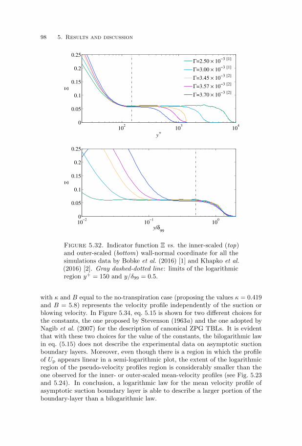
98 5. Results and discussion
102
103
104
0
0.05
0.1
0.15
0.2
0.25
y+
Ξ
10−2
10−1
100
0
0.05
0.1
0.15
0.2
0.25
y/δ99
ΞΓ=2.50 × 10
−3 [1]
Γ=3.00 × 10⁻³
[1]
Γ=3.45 × 10⁻³
[2]
Γ=3.57 × 10⁻³
[2]
Γ=3.70 × 10⁻³
[2]
Figure 5.32. Indicator function Ξ vs. the inner-scaled (top)and outer-scaled (bottom) wall-normal coordinate for all thesimulations data by Bobke et al. (2016) [1] and Khapko et al.(2016) [2]. Gray dashed-dotted line: limits of the logarithmicregion y+ = 150 and y/δ99 = 0.5.
with κ and B equal to the no-transpiration case (proposing the values κ = 0.419and B = 5.8) represents the velocity profile independently of the suction orblowing velocity. In Figure 5.34, eq. 5.15 is shown for two different choices forthe constants, the one proposed by Stevenson (1963a) and the one adopted byNagib et al. (2007) for the description of canonical ZPG TBLs. It is evidentthat with these two choices for the value of the constants, the bilogarithmic lawin eq. (5.15) does not describe the experimental data on asymptotic suctionboundary layers. Moreover, even though there is a region in which the profileof Up appears linear in a semi-logarithmic plot, the extent of the logarithmicregion of the pseudo-velocity profiles region is considerably smaller than theone observed for the inner- or outer-scaled mean-velocity profiles (see Fig. 5.23and 5.24). In conclusion, a logarithmic law for the mean velocity profile ofasymptotic suction boundary layer is able to describe a larger portion of theboundary-layer than a bilogarithmic law.
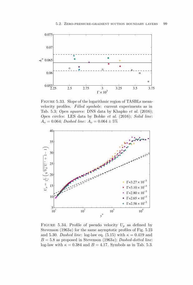
5.2. Zero-pressure-gradient suction boundary layers 99
2.25 2.5 2.75 3 3.25 3.5 3.750.055
0.06
0.065
0.07
0.075
Γ × 103
Ao
Figure 5.33. Slope of the logarithmic region of TASBLs mean-velocity profiles. Filled symbols: current experiments as inTab. 5.3; Open squares: DNS data by Khapko et al. (2016);Open circles: LES data by Bobke et al. (2016); Solid line:Ao = 0.064; Dashed line: Ao = 0.064± 5%
101
102
103
104
5
10
15
20
25
30
35
40
y+
Up=
2
V+ 0
(
√
V+ 0U
++
1−
1
)
Γ=3.27 × 10⁻³
Γ=3.10 × 10⁻³
Γ=2.80 × 10⁻³
Γ=2.65 × 10⁻³
Γ=2.58 × 10⁻³
Figure 5.34. Profile of pseudo velocity Up as defined byStevenson (1963a) for the same asymptotic profiles of Fig. 5.23and 5.30. Dashed line: log-law eq. (5.15) with κ = 0.419 andB = 5.8 as proposed in Stevenson (1963a); Dashed-dotted line:log-law with κ = 0.384 and B = 4.17. Symbols as in Tab. 5.3.

100 5. Results and discussion
5.2.5. Profiles of streamwise velocity variance
In Figure 5.35 the profiles of streamwise-velocity variance for the turbulentasymptotic cases measured at x = 4.8 m are plotted and compared with onenon-transpired ZPG TBL. The ZPG TBL profile chosen for the comparisonhas a Reynolds number Reτ = 4470, comparable to the two TASBLs with thelowest suction rates (Reτ = 4220 and 4720). It is evident that wall-normalsuction strongly damps the intensity of the velocity fluctuations in the wholeboundary layer. The shape of the velocity-variance profile is also significantlyaltered: an inner-peak is still observable close to the wall but the “shoulder”observable in the overlap region of canonical ZPG TBLs (which becomes morepronounced at larger Reynolds numbers) disappears, replaced by a monotonicdecrease from the inner peak to the boundary-layer edge.
In the profiles considered, however, the large wall shear stress leads toinsufficient spatial resolution of the hot-wire probe, with L+
w = 65− 80. Thetemporal resolution of the measurement is also insufficient for temporally fully-resolved measurement, with values of 1/f+max, where fmax is the largest resolvedfrequency, exceeding the criterion 1/f+max < 3 proposed by Hutchins et al. (2009).In order to overcome these limitations, a series of velocity profiles was measuredwith the wall-mounted traverse system at x = 6.06 m using hot-wire probeswith smaller wire-length and wire-diameter, increasing hence both the spatialand temporal resolution. For each value of Γ considered, the measurement hasbeen repeated with three different hot-wire probes, in order to quantify andcorrect for the spatial filtering effects. Moreover the experimental conditionswere chosen such that matching values of L+
w could be obtained for differentvalues of Γ in order to allow for direct comparison between profiles at differentsuction rates. The experimental parameters for this set of experiments arelisted in Table 5.4. Since just one velocity profile at a fixed streamwise locationhas been obtained, the term dθ/dx of the von-Karman momentum-integralspecialized for boundary-layer with wall transpiration
Cf2
=dθ
dx− V0U∞
(5.16)
remains unknown. For all the suction cases reported in §5.2.3, however, inthe region x > 4.0 m, dθ/dx < 0.02 × |V0/U∞|. Since the measurement casesconsidered in this section are similar for suction rate and suction start-locationto those in §5.2.3, the additional systematic error on the wall shear stressintroduced by neglecting the momentum-thickness derivative can hence beestimated to be less than 2% in Cf or less than 1% in uτ . To assess whether thevelocity profile measured are representative of asymptotic states, in Figure 5.36the mean-velocity profiles are compared with the log law proposed in §5.2.4(eq. 5.7). Good agreement with the proposed scaling is observed for all theprofiles, with somewhat larger deviation for the cases with Γ ≈ 2.56 (yellowsymbols), suggesting that the asymptotic state is just approximated but notfully obtained for this suction rate.

5.2. Zero-pressure-gradient suction boundary layers 101
101
102
103
104
0
0.5
1
1.5
2
2.5
y+
u′2+
101
102
103
104
0
2
4
6
8
Γ=3.27 × 10⁻³
; Lw
+ = 80
Γ=3.10 × 10⁻³
; Lw
+ = 78
Γ=2.80 × 10⁻³
; Lw
+ = 64
Γ=2.65 × 10⁻³
; Lw
+ = 75
Γ=2.56 × 10⁻³
; Lw
+ = 79
Γ = 0; Reτ = 5250; L
w
+ = 19
Figure 5.35. Symbols: Inner-scaled velocity-variance profilesat x = 4.8 m for TASBLs at various suction rates. Symbols asin Tab. 5.3. In the inset a comparison with one of the canonicalZPG TBL case reported in Fig. 5.8 with Reτ = 5250.
10−3
10−2
10−1
100
101
0.4
0.5
0.6
0.7
0.8
0.9
1
y/δ99
U/U
∞
Figure 5.36. Outer-scaled mean-velocity profile measured atx = 6.06 m. Dashed line: log law as in eq. (5.7) with Ao = 0.064and Bo = 0.994. Symbols as in Tab. 5.4: the same color is usedfor cases with matching suction rate.

102
5.
Resu
lts
and
disc
ussio
nTable 5.4. Experimental parameters for the suction cases at x = 6.06 m.
Case
U∞ (m/s) 34.0 34.1 34.1 34.9 35.0 35.0 37.5 37.3 37.5 38.0 38.1 37.7 39.1 38.8 38.9−V0 (m/s) 0.127 0.127 0.126 0.120 0.120 0.122 0.109 0.109 0.109 0.104 0.103 0.104 0.100 0.100 0.100Γ× 103 (-) 3.74 3.72 3.70 3.44 3.43 3.48 2.90 2.92 2.90 2.72 2.71 2.75 2.55 2.57 2.57xs (m) 0.19 0.19 0.19 0.30 0.30 0.30 0.94 0.94 0.94 1.24 1.24 1.25 1.24 1.24 1.25Rex,s × 10−6 (-) 0.43 0.43 0.43 0.70 0.71 0.69 2.31 2.28 2.29 3.13 3.14 3.13 3.22 3.20 3.23uτ (m/s) 2.08 2.08 2.07 2.05 2.05 2.07 2.02 2.02 2.02 1.99 1.99 1.98 1.98 1.97 1.97Cf × 103 (-) 7.47 7.44 7.40 6.88 6.87 6.97 5.81 5.84 5.81 5.45 5.42 5.49 5.10 5.13 5.14`∗ (µm) 7.3 7.3 7.2 7.4 7.3 7.4 7.5 7.6 7.6 7.6 7.6 7.6 7.6 7.6 7.6θ (mm) 0.52 0.54 0.54 0.81 0.85 0.82 1.76 1.84 1.83 2.24 2.28 2.27 2.52 2.55 2.41δ∗ (mm) 0.64 0.66 0.66 0.98 1.02 0.99 2.06 2.15 2.14 2.62 2.66 2.65 2.96 2.98 2.83δ99 (mm) 8.23 8.83 8.62 13.25 13.97 13.51 29.63 31.63 31.71 36.84 36.80 38.14 39.19 39.25 38.38Reθ (-) 1170 1210 1220 1890 1970 1880 4340 4480 4490 5660 5780 5710 6560 6590 6240Reτ (-) 1130 1220 1190 1800 1900 1820 3940 4150 4180 4860 4860 5010 5140 5130 5040H12 (-) 1.23 1.23 1.22 1.21 1.20 1.20 1.17 1.17 1.17 1.17 1.17 1.17 1.17 1.17 1.18Lw (mm) 0.57 0.41 0.23 0.57 0.41 0.23 0.57 0.41 0.23 0.57 0.41 0.23 0.57 0.41 0.23L+w (-) 78 56 32 77 55 31 76 53 30 75 54 30 75 53 30
1/f+max (-) 9.5 3.6 3.6 9.3 3.5 3.5 8.9 3.3 3.3 8.7 3.3 3.2 8.6 3.2 3.2tsmpU∞δ99
(-) 248100 231400 237100 158200 150100 155400 75900 70800 70900 62000 62200 59300 59900 59300 60900

5.2. Zero-pressure-gradient suction boundary layers 103
Figure 5.37 illustrates the dependency of the measured inner-scaled velocityvariance profile to the viscous-scaled wire length for all the cases at x = 6.06 m.The correction method proposed by Segalini et al. (2011) has been applied onthe measured data in order to compensate for filtering effects and obtain anestimate of the actual velocity-variance profile. The correction scheme relieson the dependence of the spatially-averaged streamwise turbulence intensityon the wire length and on the spanwise correlation coefficient (Dryden et al.1937), which in turn can be related to the local transverse Taylor microscale(Frenkiel 1949; Segalini et al. 2011): if the same flow field is measured withtwo or more hot-wire length, an estimate of the actual velocity variance canbe obtained together with an estimate of the Taylor microscale. The resultsof the correction method are reported in Figure 5.37 for all the suction ratesinvestigated. Even though other correction methods for hot-wire spatial filteringexist (Monkewitz et al. 2010; Smits et al. 2011), they were developed andcalibrated for wall-bounded flow in absence of wall transpiration and cannothence be applied on turbulent suction boundary layers.
Figure 5.38 reports, for all the suction rates considered, the inner-scaledvelocity variance profiles corrected from spatial-filtering effects, together withthe measured profile at matched L+
w ≈ 31 for the suction cases. Figure 5.38 alsodepicts a comparison with DNS and experimental corrected and uncorrectedvelocity-variance profiles for canonical ZPG-TBLs. The velocity variance isstrongly damped by the suction if compared to a canonical ZPG TBL, asalready noted in Figure 5.35. For the suction rates investigated the reductionof the (corrected) near-wall peak ranges from about 50% to 65% in respect to acanonical ZPG TBL with approximately the same Reτ . The magnitude of thenear-wall peak of the inner-scaled velocity variance profile is clearly dependenton the suction rate, with larger peak value for lower suction rates. The variationof the velocity-variance peak with the suction rate is reported in Figure 5.40in inner and outer scaling and compared with numerical simulations results byBobke et al. (2016) and Khapko et al. (2016). A simple linear fit through the
experimental data (u′2+
peak = −1170 Γ + 7.18) describes reasonably well (max.deviation < 2.5%) the inner-scaled velocity-variance peak from the currentexperiment and from the LES by Bobke et al. (2016), but not from the DNSby Khapko et al. (2016). In the range of suction rates considered, the velocityvariance peak from the experiments and the LES (but not from the DNS) can
also be described with the same accuracy by the relation u′2peak/U2∞ = 0.0108.
Since for an asymptotic state
u′2+
=u′2
−U∞V0=
u′2
U2∞
1
Γ, (5.17)
these two simple empirical relations are in contradiction with each other andwill diverge for decreasing suction ratio. From eq. (5.17) it is also apparent that
if u′2peak/U2∞ is taken as constant, u′2
+
peak →∞ if Γ→ 0, which is unphysical.

104 5. Results and discussion
0
0.5
1
1.5
2
2.5
3
3.5
4
4.5
Γ = 3.72 × 10⁻³
u′2+
Lw
+ = 32
Lw
+ = 56
Lw
+ = 78
Γ = 3.45 × 10⁻³
Lw
+ = 31
Lw
+ = 55
Lw
+ = 77
0
0.5
1
1.5
2
2.5
3
3.5
4
4.5
Γ = 2.91 × 10⁻³
u′2+
Lw
+ = 30
Lw
+ = 53
Lw
+ = 76
101
102
103
104
Γ = 2.73 × 10⁻³
y+
Lw
+ = 30
Lw
+ = 54
Lw
+ = 75
101
102
103
104
0
0.5
1
1.5
2
2.5
3
3.5
4
4.5
Γ = 2.56 × 10⁻³
y+
u′2+
Lw
+ = 30
Lw
+ = 53
Lw
+ = 75
Figure 5.37. Inner-scaled velocity-variance profiles at x =6.06 m for different suction rates. Symbols: measured data forvarious hot-wire length L+
w ; Colored lines : data corrected fromspatial-filtering effects with the method by Segalini et al. (2011)using all three measured profiles (dashed lines) and using justdata measured with the smallest and the largest probe (solidlines).

5.2. Zero-pressure-gradient suction boundary layers 105
101
102
103
104
0
1
2
3
4
5
6
7
8
9
y+
u′2+
Γ × 10
3 = 2.57, Re
τ = 5040
Γ × 103 = 2.75, Re
τ = 5010
Γ × 103 = 2.90, Re
τ = 4180
Γ × 103 = 3.48, Re
τ = 1820
Γ × 103 = 3.70, Re
τ = 1190
Γ = 0, Reτ = 5250
Γ = 0, Reτ = 1145
Figure 5.38. Inner-scaled velocity-variance profiles at x =6.06 m for different suction rates compared with no-transpiration cases. Circles: TASBLs (measured data, L+
w ≈31); Solid lines: TASBLs, corrected data (method: Segaliniet al. 2011); Triangles: canonical ZPG TBL at Reτ = 5250(measured data, L+
w ≈ 19); Dashed-dotted line: canonical ZPGTBL at Reτ = 5250, corrected data (method: Smits et al.2011); Dashed line: canonical ZPG TBL at Reτ = 1145, DNS
by Schlatter & Orlu (2010)
From Figure 5.38 we observe that the streamwise velocity-variance profilesdecrease monotonically from the inner-peak location to the zero value at theboundary-layer edge. For non-transpired canonical boundary layers (canonicalZPG TBL, turbulent pipe flow and turbulent channel flow) a shoulder in theouter part of the inner-scaled velocity-variance profiles is present and it becomesmore evident with increasing Reynolds number, finally taking the shape of aplateau for high enough Reynolds numbers3. It has been shown (Marusic et al.2010; Ng et al. 2011) that this increase with Reynolds-number of the magnitudeof the broadband velocity-variance profiles in the outer region can be attributedto the large and very-large scale motions. It can be speculated, based on thepresent data, that even small values of wall suction such as those applied inthis experiment are very effective in reducing the strength of the larger scalesof a turbulent boundary layer. This tentative conclusion finds support in theanalysis of the frequency spectra of the velocity signal (see §5.2.6).
3Whether or not an outer peak of the streamwise-velocity variance appears at high enoughReynolds number is a matter of debate, see e.g. Hutchins et al. (2009), Vallikivi et al. (2015)
and Monkewitz & Nagib (2015).

106 5. Results and discussion
0 0.2 0.4 0.6 0.8 1 1.2 1.40
0.002
0.004
0.006
0.008
0.01
y/δ99
u′2 /U
2 ∞
Γ × 10
3 = 2.57, Re
τ = 5040
Γ × 103 = 2.75, Re
τ = 5010
Γ × 103 = 2.90, Re
τ = 4180
Γ × 103 = 3.48, Re
τ = 1820
Γ × 103 = 3.70, Re
τ = 1190
Γ = 0, Reτ = 5250
Γ = 0, Reτ = 1145
Figure 5.39. Outer-scaled velocity-variance profiles atx = 6.06 m for different suction rates compared with no-transpiration cases. Circles: TASBLs (measured data, L+
w ≈31); Triangles : canonical ZPG TBL, measured data (L+
w ≈ 19);
Dashed line: canonical ZPG TBL, DNS by Schlatter & Orlu(2010)
The outer-scaled velocity-variance profiles, reported in Figure 5.39, show agood overlap for a large portion of the boundary-layer thickness (y/δ99 > 0.2)for all the profiles excluding the case with Γ = 2.57. For this particular case,however, the full achievement of the asymptotic state was considered doubtfulfrom the analysis of the mean velocity profile. The observed similarity betweenouter-scaled velocity variance profiles at different suction rates is howeverin contradiction with the outer-scaled similarity of the mean-velocity profileproposed in §5.2.4. Recalling eq. (2.41), describing the Reynolds shear-stressdistribution in the outer region of a TASBL, a similarity between the outer-scaled streamwise mean velocity profile of TASBL at different suction rates
implies a similarity between the viscous scaled Reynolds stress −u′v′+ (andvice versa), giving
U
U∞= f1(η) ⇐⇒ −u′v′+ = 1− f1(η) . (5.18)
For consistency with the proposed similarity of the mean-velocity profile inouter-scaled variables (see §5.2.4) and considering that the various components ofthe Reynolds-stress tensor should share the same scaling if similarity is observed,
it is expected that u′2+
= f(η). In Figure 5.41 the inner- and outer-scaledvelocity-variance profiles are plotted vs. the outer-scaled wall-normal distancefor the current experiments and the simulations data by Bobke et al. (2016)

5.2. Zero-pressure-gradient suction boundary layers 107
2.5 2.7 2.9 3.1 3.3 3.5 3.7 3.92
2.5
3
3.5
4
4.5
5
(
u′2+)
peak
Γ × 103
2.5 2.7 2.9 3.1 3.3 3.5 3.7 3.90.008
0.009
0.01
0.011
0.012
Γ × 103
(
u′2 /U
2 ∞
)
peak
Figure 5.40. Maximum of the velocity variance in inner (top)and outer (bottom) scaling. Open circles: current experiments,measured data for L+
w ≈ 31; Filled circles : current experiments,corrected data (method by Segalini et al. 2011); Blu squares:LES simulations by Bobke et al. (2016); Red diamonds: DNSsimulations by Khapko et al. (2016); Black dashed-dotted line:linear fit through the experimental data; Red dashed-dottedline: u′2/U2
∞ = 0.0108; Vertical dashed line: self-sustainedturbulence threshold (Khapko et al. 2016).
and Khapko et al. (2016). The experimental data show larger scatter if innerscaling is adopted, in apparent contradiction with the observed behaviour ofthe mean-velocity profiles. However, the opposite is observed for the simulation
data, for which good scaling of u′2+
occurs in the region (y/δ99 > 0.4) for allthe suction rates excluding the lowest (Γ = 2.50 × 10⁻³). The reason of thisdiscrepancy between experiments and simulations is at the present state unclear,even though it can be hypothesized that, analogously to what happen in pipeflow (Doherty et al. 2007), the achievement of a fully developed (asymptotic)turbulent state for the velocity-variance profile requires a longer streamwisedistance than for the mean-velocity profile.

108 5. Results and discussion
0 0.2 0.4 0.6 0.8 1 1.20
0.5
1
1.5
2x 10
−3
y/δ99
u′2 /U
2 ∞
0 0.2 0.4 0.6 0.8 1 1.20
0.1
0.2
0.3
0.4
0.5
0.6
0.7
0.8
y/δ99
u′2+
Γ = 2.57 × 10⁻³
Γ = 2.75 × 10⁻³
Γ = 2.90 × 10⁻³
Γ = 3.48 × 10⁻³
Γ = 3.70 × 10⁻³
Γ = 2.50 × 10⁻³
[1]
Γ = 3.00 × 10⁻³
[1]
Γ = 3.45 × 10⁻³
[2]
Γ = 3.57 × 10⁻³
[2]
Γ = 3.70 × 10⁻³
[2]
Figure 5.41. Outer- (left) and inner- (right) scaled velocityvariance profiles for the current experiments (symbols) andavailable numerical simulations ([1]: Bobke et al. (2016); [2]:Khapko et al. (2016)).
Given the small amount of experimental or numerical data on TASBLs,firm conclusion on the scaling of the velocity variance in TASBL should waitfor data covering a larger range of suction rates (and hence Reτ ) from moreindependent sources. If a Reynolds-number similarity of the Reynolds-stressestensor is confirmed for this flow, it would constitute a solid ground to explainthe observed outer scaling of the mean-velocity profile, as apparent from theexpression 5.18, derived form the Navier-Stokes equations for a 2D TASBL withthe only assumption of negligible viscous stress.
5.2.6. Spectra
Figure 5.42 depicts the inner-scaled premultiplied power-spectral-density (P.S.D.)map for all the suction cases for x = 6.06 m obtained with matching L+
w ≈ 31.The P.S.D. were estimated from the streamwise-velocity time series using Welch’smethod (Welch 1967). The wavelengths were inferred from the time-series ofvelocity using the Taylor’s “frozen turbulence” hypothesis (Taylor 1938) and thelocal mean velocity as the convective velocity of the waves. The applicabilityof Taylor’s hypothesis to wall-bounded flows has been recently questioned:Del Alamo & Jimenez (2009) showed with DNS of turbulent channel flow thatthe hypothesis holds for the small eddies (except near the wall), but is violatedby eddies with long wavelength, which are advected at velocity close to the bulkvelocity. For suction boundary layers, as can be observed from Figure 5.42, theenergetic contribution of the low frequency (large wavelength) components is

5.2. Zero-pressure-gradient suction boundary layers 109
small compared to the high frequency ones, providing a justification for theapplication of Taylor’s hypothesis.
As conjectured from the analysis of the velocity variance profiles, suctionis very effective in reducing the strength of the large scale structures presentin turbulent boundary layers, so that TASBLs (at least at the suction ratesconsidered) appear to be fundamentally dominated by the near-wall cycle. Thisis particularly evident if the power-spectra maps of the two lowest suction casesare compared with a canonical ZPG TBL at comparable Reτ (Fig. 5.43), forwhich a clear contribution of the large energy components is observed in a largeportion of the boundary-layer.
The streamwise wavelength λ+x,p related to the peak of the premultipliedpower spectral density increases with the suction rates, as clearly illustratedin Figure 5.44. For the non-transpired case the peak in f+P+
uu occurs atλ+x,p ≈ 1000 (in agreement with Jimenez et al. 2004; Hutchins & Marusic 2007
among others) and it increases with the suction rate reaching λ+x,p ≈ 2700
for Γ = 3.70 × 10⁻³. The peak in the premultiplied power spectral densitycorresponds to the signature of near-wall motion of the high- and low-speedstreaks observed firstly by Kline et al. 1967. The increase of the λ+x,p with thesuction rate is hence in qualitative agreement with the measurements and flowvisualization of a (localized) suction boundary layer by Antonia et al. (1988),who reported that “low-speed streaks tend to oscillate less in a spanwise directionwhile their streamwise persistence is increased [compared to the non transpiredcase]”. Since the instability of the near-wall streaks plays a major role in theproduction of turbulence (see Kim et al. 1971; Jimenez & Pinelli 1999, amongothers), the increased stability of the near-wall streaks was related by Antoniaet al. (1988) to the decrease of the Reynolds stresses in presence of wall-normalsuction.
5.2.7. Higher order moments
To conclude this description of turbulent suction boundary layers, the profilesof skewness and kurtosis of the streamwise velocity are reported for the suctioncases at x = 6.06 m and compared with canonical ZPG TBLs at different Reτin Figure 5.45 and 5.46 respectively. In the inner region of the boundary layer,the skewness of the velocity becomes more negative with increasing suctionrates, meaning that in this region the ejections of low momentum fluid fromthe wall are more frequent than sweeps of high momentum fluid from the outerpart of the boundary layer. This observation is in accordance with the viewof turbulent suction boundary layers (at least in the range of Reτ considered)as fundamentally dominated by the near wall cycle deducted from the analysisof the spectral maps. Similarly, the increase of the near-wall minimum valueof the skewness profile with increasing Reτ for the canonical ZPG-TBL casescan be related to the more frequent sweeps of high-momentum fluids towardthe near-wall region caused by the larger relevance for increasing Reynoldsnumber of the outer large-scale motions. For the suction cases the near-wall

110 5. Results and discussion
Figure 5.42. Premultiplied power-spectral-density maps ininner scaling for the suction cases measured at x = 6.06 m withmatching L+
w ≈ 31.

5.2. Zero-pressure-gradient suction boundary layers 111
Figure 5.43. Premultiplied power-spectral-density maps ininner scaling for the ZPG TBL case measured at x = 6.06 mwith Reτ = 5250 and L+
w ≈ 19.
101
102
103
104
105
0
0.2
0.4
0.6
0.8
1
1.2
1.4
1.6
1.8
2
λx
+
f + S
uu
+
y+ ≈ 15
Γ = 3.70 × 10⁻³
Γ = 3.48 × 10⁻³
Γ = 2.90 × 10⁻³
Γ = 2.75 × 10⁻³
Γ = 2.57 × 10⁻³
Γ = 0
Figure 5.44. Premultiplied power-spectral-density maps ininner scaling for y+ ≈ 15 and x = 6.06 m. Colored lines:suction cases with L+
w ≈ 31; Black line: canonical ZPG TBLwith Reτ = 5250 and L+
w ≈ 19.

112 5. Results and discussion
101
102
103
104
−3
−2.5
−2
−1.5
−1
−0.5
0
0.5
1
y+
Sk u
’
Γ × 10
3 = 2.57, Re
τ = 5040
Γ × 103 = 2.75, Re
τ = 5010
Γ × 103 = 2.90, Re
τ = 4180
Γ × 103 = 3.48, Re
τ = 1820
Γ × 103 = 3.70, Re
τ = 1190
Γ = 0; Reτ = 5250; L
w
+ = 19
Γ = 0; Reτ = 2500; L
w
+ = 8
Γ = 0, Reτ = 1145; DNS
Figure 5.45. Velocity-skewness profiles at x = 6.06 m for thesuction cases and for canonical ZPG TBLs. Circles: TASBLs(L+
w ≈ 31); Black symbols : canonical ZPG TBL, measured data;
Dashed line: canonical ZPG TBL, DNS by Schlatter & Orlu(2010)
minimum of the skewness profile becomes more negative with increasing suctionrate, while its location moves outwards, with values ranging from y+ ≈ 40 forΓ = 2.57× 10⁻³ to y+ ≈ 60 for Γ = 3.70× 10⁻³.
The velocity-kurtosis profiles of the suction cases show a near-wall peakincreasing in magnitude with the suction rate. Its wall-normal location increaseswith the suction rate, with values ranging from y+ ≈ 70 for Γ = 2.57× 10⁻³ toy+ ≈ 85 for Γ = 3.70×10⁻³. The distinctive minimum and distinctive maximumobserved respectively for the skewness and flatness profile in correspondence ofthe boundary-layer edge are indicators of the highly intermittent behaviour ofthe flow in this region. As a final observation, the smoothness of the skewnessand kurtosis profile serves as a proof that the sampling time chosen for themeasurement was long enough to obtain well-converged statistics.

5.2. Zero-pressure-gradient suction boundary layers 113
101
102
103
104
2
10
20
30
y+
Ku
u’
Γ × 10
3 = 2.57, Re
τ = 5040
Γ × 103 = 2.75, Re
τ = 5010
Γ × 103 = 2.90, Re
τ = 4180
Γ × 103 = 3.48, Re
τ = 1820
Γ × 103 = 3.70, Re
τ = 1190
Γ = 0; Reτ = 5250; L
w
+ = 19
Γ = 0; Reτ = 2500; L
w
+ = 8
Γ = 0, Reτ = 1145; DNS
Figure 5.46. Velocity-kurtosis profiles at x = 6.06 m for thesuction cases and for canonical ZPG TBLs. Circles: TASBLs(L+
w ≈ 31); Black symbols : canonical ZPG TBL, measured data;
Dashed line: canonical ZPG TBL, DNS by Schlatter & Orlu(2010); Solid line: normal-distribution kurtosis Kuu′ = 3.

114 5. Results and discussion
5.3. Zero-pressure-gradient turbulent blowing boundarylayers
A series of blowing boundary-layer profiles was measured at the most downstreammeasurement location (x = 6.06 m). For all the measurement cases uniform blow-ing was applied in the whole region downstream of the first plate element (xs =0.94 m). The blowing rates considered were Γ ≈ (1.00; 1.46; 1.95; 2.95; 3.74)×10−3
and for each blowing rate boundary layers with different Re number were ob-tained regulating the free-stream velocity in the range from 10 m/s to 40 m/s.The experimental parameters for the measurements of blowing boundary layersare listed in Table 5.5. To assess the magnitude of the spatial filtering of thehot-wire probe, selected measurements were repeated with a different wirelength. Unfortunately, given the difficulties in measuring the shear-stress in aboundary layer with transpiration (see §3.7.2 and §3.7.3), the friction velocitycould not be estimated for these experiments, hence all the results will bepresented exclusively in outer scaling. No boundary-layer separation could beobserved by means of tufts visualization for the whole range of blowing ratesand Reynolds numbers considered.
Table 5.5. Experimental parameters for all the blowing tur-bulent boundary layers measured at x = 6.06 m
Case U∞ V0 Γ× 103 xs Rex,s × 10−6 θ δ∗ δ99 Reθ H12 LwtsmpU∞δ99
(m/s) (m/s) (-) (m) (-) (mm) (mm) (mm) (-) (-) (mm) (-)
39.9 0.039 0.98 0.94 2.40 12.05 16.53 97.73 30820 1.37 0.57 32700
39.9 0.039 0.98 0.94 2.41 11.73 16.11 94.88 30130 1.37 0.28 33700
30.0 0.029 0.97 0.94 1.82 12.41 17.14 98.87 24130 1.38 0.28 27300
20.0 0.019 0.97 0.94 1.21 12.56 17.62 101.34 16280 1.40 0.28 19700
15.1 0.014 0.95 0.94 0.91 12.98 18.37 102.25 12550 1.42 0.28 17700
40.0 0.060 1.49 0.94 2.41 14.07 20.03 112.15 36220 1.42 0.57 28600
39.8 0.059 1.49 0.94 2.41 14.13 19.98 110.41 36390 1.41 0.28 28800
30.0 0.044 1.47 0.94 1.83 14.19 20.29 112.91 27720 1.43 0.28 23900
19.9 0.029 1.47 0.94 1.20 14.32 20.51 106.52 18270 1.43 0.28 18600
15.0 0.022 1.46 0.94 0.91 15.02 21.67 112.50 14550 1.44 0.57 13300
10.0 0.014 1.42 0.94 0.62 15.12 22.07 110.38 9940 1.46 0.28 10900
30.1 0.059 1.97 0.94 1.83 17.02 24.99 125.41 33230 1.47 0.28 21600
30.0 0.060 2.00 0.94 1.80 17.12 25.25 125.48 32960 1.48 0.57 21500
20.0 0.039 1.97 0.94 1.20 16.65 24.58 123.12 21320 1.48 0.28 16200
15.0 0.029 1.95 0.94 0.93 16.88 25.22 124.67 16740 1.49 0.57 10800
10.1 0.019 1.91 0.94 0.62 16.83 25.33 123.26 11140 1.51 0.28 9800
20.0 0.060 3.00 0.94 1.20 21.97 34.47 150.46 28140 1.57 0.28 13300
20.0 0.059 2.96 0.94 1.22 22.09 34.58 151.68 28710 1.57 0.57 11900
15.1 0.044 2.92 0.94 0.93 21.65 34.21 152.00 21480 1.58 0.57 10400
10.0 0.029 2.93 0.94 0.61 21.43 33.91 149.56 13870 1.58 0.57 8000
16.0 0.060 3.72 0.94 0.96 25.33 41.59 175.68 26050 1.64 0.28 10900

5.3. Zero-pressure-gradient turbulent blowing boundary layers 115
5.3.1. Mean-velocity and velocity-variance profiles
Figures from 5.47 to 5.51 illustrate the measured mean-velocity profiles fordifferent blowing rates and Reθ. A comparison with the lower Reynolds-numberexperiments by Andersen et al. (1972) is presented whenever data at matchingblowing rate were available. For all the blowing rates considered excluding thelowest (Γ ≈ 1.00× 10⁻³), overlap of the outer-scaled mean velocity is observedin a large portion of the boundary layer for large enough momentum-thicknessReynolds numbers. The range of Reθ among which the the outer-scaled mean-velocity profiles overlap is increasingly larger with increasing blowing rate. Forthe largest blowing rate considered, Γ ≈ 3.74 × 10⁻³, a good overlap of theouter-scaled mean-velocity profiles is noticed for 98% of the boundary layer-thickness between Reθ = 6670 and Reθ = 26050 (see Fig. 5.51), while forΓ ≈ 2.95 × 10⁻³ the outer-scaled mean-velocity profile are indistinguishablefor the outer 99% of the boundary-layer thickness in the Reynolds numberrange from Reθ = 13870 and Reθ = 28710 (see Fig. 5.50). In absence of anestimate for the friction velocity, the variation of U+
∞ with the Reynolds numberis unknown, hence it is not possible to conclude whether scaling of the meanvelocity with U∞ is to be preferred over the scaling with uτ . For the same reason,the applicability of the bi-logarithmic law of the wall (see §2.2.4) cannot betested on the experimental database. Mean-velocity profiles at different blowingrates are compared in Figure 5.52 from which a clear dependency on the blowingrates of the outer-scaled mean-velocity profile is apparent. With increasingblowing rates, moreover, an increasing curvature of the semi-logarithmic plot ofthe mean velocity profiles becomes evident, suggesting that for this type of flowa logarithmic law cannot properly describe the mean-velocity distribution.
In Figure 5.53 the velocity-defect profiles U∞ − U normalized with theZagarola-Smits velocity scale U∞δ
∗/δ99 are plotted vs. the outer-scaled wall-normal distance for all the blowing cases measured and compared with onenon-transpired ZPG TBL case and with the TASBL cases of Table 5.3. Weobserve a good overlap between all the blowing boundary layer profiles andthe non-transpired ZPG TBL case, in agreement with Cal & Castillo (2005)and Kornilov & Boiko (2012), but not between blowing and suction profiles, asalready noted by Cal & Castillo (2005). Even if for graphical clarity Figure 5.53reports just one canonical ZPG TBL case, the above conclusions do not change ifall the measured ZPG TBL cases measured are considered. Finally, Figure 5.54shows the variation of the shape factor with the momentum-thickness Reynoldsnumber for all the measured blowing boundary layers, illustrating that theshape factor at fixed Reθ increases with the blowing rate.
Wall-normal blowing generally increases the magnitude of turbulent fluctu-ations in the whole boundary layer, as observed from Figure 5.55 showing thelocal turbulence intensity profiles for boundary layers at different blowing rates.The shape of the velocity-variance profiles is also altered by the applicationof wall-blowing, as evident from Figure 5.56, illustrating the velocity-varianceprofiles for blowing boundary layers at different blowing rates and Reynolds

116 5. Results and discussion
10−3
10−2
10−1
100
0
0.1
0.2
0.3
0.4
0.5
0.6
0.7
0.8
0.9
1
Γ ≈ 1.00 × 10⁻³
y/δ99
U/U
∞
Re
θ = 30130
Reθ = 24130
Reθ = 16280
Reθ = 12550
Reθ = 4000
[*]
Figure 5.47. Outer-scaled mean-velocity profiles for blowingboundary layers with Γ ≈ 0.97× 10⁻³. Filled Symbols : currentinvestigation, x = 6.06 m (see Tab. 5.5); (*) Open Symbols:data from Andersen et al. (1972): case 100571-1 (x = 90 in;Γ = 1.04× 10⁻³).
10−3
10−2
10−1
100
0
0.1
0.2
0.3
0.4
0.5
0.6
0.7
0.8
0.9
1
Γ ≈ 1.46 × 10⁻³
y/δ99
U/U
∞
Re
θ = 36390
Reθ = 27720
Reθ = 18270
Reθ = 14550
Reθ = 9940
Figure 5.48. Outer-scaled mean-velocity profiles for blowingboundary layers with Γ ≈ 1.47× 10⁻³, current investigation,x = 6.06 m (see Tab. 5.5).

5.3. Zero-pressure-gradient turbulent blowing boundary layers 117
10−3
10−2
10−1
100
0
0.1
0.2
0.3
0.4
0.5
0.6
0.7
0.8
0.9
1
Γ ≈ 1.95 × 10⁻³
y/δ99
U/U
∞
Re
θ = 33230
Reθ = 21320
Reθ = 16740
Reθ = 11140
Reθ = 4740
[*]
Figure 5.49. Outer-scaled mean-velocity profiles for blowingboundary layers with Γ ≈ 1.97× 10⁻³. Filled Symbols : currentinvestigation, x = 6.06 m (see Tab. 5.5); (*) Open Symbols:data from Andersen et al. (1972): case 090171-2 (x = 90 in;Γ = 2.00× 10⁻³).
10−3
10−2
10−1
100
0
0.1
0.2
0.3
0.4
0.5
0.6
0.7
0.8
0.9
1
Γ ≈ 2.95 × 10⁻³
y/δ99
U/U
∞
Re
θ = 28710
Reθ = 21480
Reθ = 13870
Figure 5.50. Outer-scaled mean-velocity profiles for blowingboundary layers with Γ ≈ 2.95× 10⁻³, current investigation,x = 6.06 m (see Tab. 5.5).

118 5. Results and discussion
10−3
10−2
10−1
100
0
0.1
0.2
0.3
0.4
0.5
0.6
0.7
0.8
0.9
1
Γ ≈ 3.74 × 10⁻³
y/δ99
U/U
∞
Re
θ = 26050
Reθ = 6670
[*]
Figure 5.51. Outer-scaled mean-velocity profiles for blowingboundary layers with Γ ≈ 3.74× 10⁻³. Filled Symbols : currentinvestigation, x = 6.06 m (see Tab. 5.5); (*) Open Symbols:data from Andersen et al. (1972): case 090871-3 (x = 90 in;Γ = 3.76× 10⁻³).
numbers: for increasing Reynolds number and fixed blowing rate the magnitudeof the inner peak decreases, while an outer peak emerges. Already for the largestReynolds number measured for Γ ≈ 1.46 × 10⁻³, the outer-peak magnitudeis larger than the magnitude of the inner-peak, and at the largest Reynoldsnumbers considered (Γ ' 2.95× 10⁻³) the inner-peak completely disappears.These observations cannot be considered an artefact caused by the spatial filter-ing of the hot-wire probe, as evident from Figure 5.57 reporting measurementsobtained with different wire-length at the largest Reynolds number consideredfor the blowing rates Γ 6 3.00×10⁻³. For Γ ≈ 2.98×10⁻³ the observed overlapof the velocity variance profiles measured with different wire-length suggests thatalready for the larger wire no significant spatial filtering occurred. For smallerblowing rates some spatial filtering effect was observed, hence the measuredvelocity variance profiles were corrected for spatial resolution effects with themethod by Segalini et al. (2011). From Figure 5.57 can be concluded that cases
( ), ( ) and ( ) can be considered free from spatial-filtering effects. This
conclusion can be extended for case ( ), characterized by the same wire-length,
larger blowing rate but smaller free-stream velocity than ( ), resulting insmaller wall shear-stress and larger `∗.
Reconsidering Figure 5.55, we observe that the near-wall turbulence intensityincreases significantly with blowing. The near-wall turbulence intensity can

5.3. Zero-pressure-gradient turbulent blowing boundary layers 119
10−3
10−2
10−1
100
0
0.1
0.2
0.3
0.4
0.5
0.6
0.7
0.8
0.9
1
y/δ99
U/U
∞
Γ = 0.98 × 10⁻³
Γ = 1.49 × 10⁻³
Γ = 1.97 × 10⁻³
Γ = 3.00 × 10⁻³
Γ = 3.72 × 10⁻³
Γ = 0
Figure 5.52. Colored symbols: mean-velocity profiles at x =6.06 m for different blowing rates at the highest Reθ measured(see Tab. 5.5). Black triangles: canonical ZPG TBL at Reθ =21330.
be related to the relative level of the wall-shear-stress fluctuations as (see e.g.Alfredsson et al. 1988) √
τ ′2w
τw= limy→0
√u′2
U. (5.19)
For the largest blowing rate measured (Γ = 3.72 × 10⁻³, in which no spatial
filtering is expected to occur), the near-wall turbulence intensity is√u′2/U ≈
0.6, about 50% larger than the value of√u′2/U ≈ 0.4 usually reported for
canonical boundary-layers (Alfredsson et al. 1988; Osterlund 1999; Alfredsson
& Orlu 2010). For suction boundary layers the opposite is observed, with thenear-wall turbulence intensity strongly damped by the suction and reaching
values of√u′2/U ≈ 0.2 for suction rate Γ = 3.70×10⁻³ (data from Khapko et al.
2016, see Fig. 4.2). In Figure 5.55 the observed value of the local turbulence
intensity at the wall for the canonical ZPG TBL case is√u′2/U ≈ 0.3, instead
of the expected value of 0.4, due to hot-wire spatial-filtering effects.
5.3.2. Spectra and higher-order statistics
Figure 5.58 reports the premultiplied power-spectral-density map for the largestReynolds number measured at each blowing rate. The results are shown in thefrequency domain instead of the wavelength domain, because, as clearly seen in

120 5. Results and discussion
0 0.2 0.4 0.6 0.8 1 1.20
1
2
3
4
5
6
y/δ99
(U∞−
U)δ
99/(U
∞δ∗)
0.2 0.4 0.6 0.8 10
0.5
1
1.5
2
y/δ99
(U∞−
U)δ
99/(U
∞δ∗)
Figure 5.53. Mean-velocity-deficit profiles for blowing, suc-tion and no-transpiration cases normalized according to Za-garola & Smits (1998a). Filled colored symbols : all the blowingboundary layers in Tab. 5.5. Black triangles: canonical ZPGTBL at Reθ = 21330. Open colored symbols: all the TASBLcases in Tab. 5.3. Inset : detail view of the outer region.
Figure 5.58 low-frequency components in the outer part of the boundary layer(representative of the large-scale motions) becomes predominant with increasingblowing rate. This observation rises doubts about the applicability of Taylor’shypothesis (see §5.2.6) for boundary layers with blowing. With increasingblowing rate, the high-frequency near-wall peak of the premultiplied P.S.D.,trace of the near-wall cycle, disappears, in agreement with the disappearance ofthe inner peak of the streamwise-velocity-variance profiles. The outer peak ofthe premultiplied P.S.D. starts to develop at wall normal location y/δ99 ≈ 0.05and normalized frequency F ≈ 0.15, spreading with increasing blowing ratestowards the outer portion of the boundary layers covering a wider frequencyrange. This observations are the opposite behaviour of what observed for suctionboundary layers, where the turbulent activity remained fundamentally limitedto the near-wall region.
The skewness and kurtosis profiles for the largest Reynolds number measuredat each blowing rate are reported and compared with canonical ZPG TBLsin Figure 5.59 and Figure 5.60 respectively. The near-wall minimum of theskewness profile observed for the canonical ZPG TBL cases disappears for theblowing boundary layers, replaced by a monothonic increase of the velocity-skewness profile. Positive values of skewness in the whole inner region are

5.3. Zero-pressure-gradient turbulent blowing boundary layers 121
5 10 15 20 25 30 35 401.2
1.3
1.4
1.5
1.6
1.7
Reθ × 10
−3
H12
Γ = 0
Γ ≈ 1.00 × 10⁻³
Γ ≈ 1.46 × 10⁻³
Γ ≈ 1.95 × 10⁻³
Γ ≈ 2.95 × 10⁻³
Γ ≈ 3.72 × 10⁻³
Figure 5.54. Shape factor H12 variation with the momentum-thickness Reynolds number Reθ for the blowing boundary layerin Tab. 5.5 (symbols) compared with the shape factor of the com-posite profile for canonical ZPG TBLs proposed by Chauhanet al. (2009) (solid line).
observed for the blowing boundary layers, indicating the prevalence of sweepingmotion of high-momentum fluid from the outer layer towards the near-wallregion, commonly associated with large-scale motions.
The streamwise-velocity-kurtosis profiles of blowing boundary layers andcanonical ZPG TBLs show a good overlap in a large portion of the boundarylayer independently of the blowing rate if plotted vs. the outer-scaled wallnormal distance. In the near-wall region, instead, differences among cases atdifferent blowing rates can be observed, with increasing values of the near-wallkurtosis for larger blowing rates. For wall normal distances 0.03 / y/δ99 / 0.3the kurtosis values is approximately constant, with a value of Kuu′ ≈ 2.7, closeto Kuu′ ≈ 2.8 reported by Fernholz & Finley (1996) for the log law regionof canonical ZPG TBL. In this respect, considerable difference in the velocitykurtosis profiles of suction boundary layers (see Fig. 5.46) can be observed: atlarge suction rate (Γ ' 3.5× 10⁻³), in fact, the value of Kuu′ remains largerthan the Gaussian value Ku = 3 in the region y+ > 40.

122 5. Results and discussion
10−3
10−2
10−1
100
0
0.1
0.2
0.3
0.4
0.5
0.6
y/δ99
√
u′2 /U
Γ = 0.98 × 10⁻³
Γ = 1.49 × 10⁻³
Γ = 1.97 × 10⁻³
Γ = 3.00 × 10⁻³
Γ = 3.72 × 10⁻³
Γ = 0
Figure 5.55. Colored symbols : local turbulence-intensity pro-files at x = 6.06 m for different blowing rates at the highestReθ measured (see Tab. 5.5). Black triangles: canonical ZPGTBL at Reθ = 21330 (L+
w ≈ 25). Data are not corrected forspatial filtering.

5.3. Zero-pressure-gradient turbulent blowing boundary layers 123
0
0.002
0.004
0.006
0.008
0.01
0.012L
w = 0.28 mmΓ ≈ 1.00 × 10
−3
u′2/U
2 ∞
Reθ = 30130
Reθ = 24130
Reθ = 16280
Reθ = 12550
Lw
= 0.28 mmΓ ≈ 1.46 × 10⁻³
Reθ = 36390
Reθ = 27720
Reθ = 18270
Reθ = 9940
0
0.002
0.004
0.006
0.008
0.01
0.012L
w = 0.28 mmΓ ≈ 1.95 × 10
−3
u′2/U
2 ∞
Reθ = 33230
Reθ = 21320
Reθ = 11140
10−3
10−2
10−1
100
Lw
= 0.57 mmΓ ≈ 2.95 × 10⁻³
y/δ99
Reθ = 28710
Reθ = 21480
Reθ = 13870
10−3
10−2
10−1
100
0
0.002
0.004
0.006
0.008
0.01
0.012L
w = 0.28 mmΓ = 3.72 × 10
−3
y/δ99
u′2 /U
2 ∞
Reθ = 26050
Figure 5.56. Outer-scaled velocity-variance profiles for blow-ing boundary layers measured at x = 6.06 m (see Tab. 5.5).
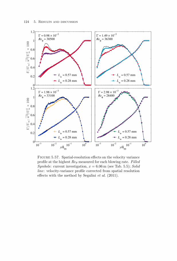
124 5. Results and discussion
0
0.2
0.4
0.6
0.8
1
1.2
Lw
= 0.57 mm
Lw
= 0.28 mm
Γ ≈ 0.98 × 10⁻³
Reθ ≈ 30500
U/U
∞;u′2 /U
2 ∞×
100
Lw
= 0.57 mm
Lw
= 0.28 mm
Γ ≈ 1.49 × 10⁻³
Reθ ≈ 36300
10−3
10−2
10−1
100
0
0.2
0.4
0.6
0.8
1
1.2
Lw
= 0.57 mm
Lw
= 0.28 mm
Γ ≈ 1.98 × 10⁻³
Reθ ≈ 33100
y/δ99
U/U
∞;u′2 /U
2 ∞×
100
10−3
10−2
10−1
100
Lw
= 0.57 mm
Lw
= 0.28 mm
Γ ≈ 2.98 × 10⁻³
Reθ ≈ 28400
y/δ99
Figure 5.57. Spatial-resolution effects on the velocity varianceprofile at the highest Reθ measured for each blowing rate. FilledSymbols : current investigation, x = 6.06 m (see Tab. 5.5); Solidline: velocity-variance profile corrected from spatial resolutioneffects with the method by Segalini et al. (2011).

5.3. Zero-pressure-gradient turbulent blowing boundary layers 125
Figure 5.58. Premultiplied power-spectral-density maps inouter scaling (F = fδ99/U∞; Puu,n = Puu/U
2∞) for the blowing
boundary layers at the highest Reτ measured for each blowingrate.

126 5. Results and discussion
10−3
10−2
10−1
100
−3
−2.5
−2
−1.5
−1
−0.5
0
0.5
1
1.5
y/δ99
Sk u
’
Γ = 0.98 × 10⁻³
Γ = 1.49 × 10⁻³
Γ = 1.97 × 10⁻³
Γ = 3.00 × 10⁻³
Γ = 3.72 × 10⁻³
Γ = 0; Reτ = 5250
Γ = 0; Reτ = 2500
Figure 5.59. Velocity-skewness profiles for the blowing bound-ary layers shown in Fig. 5.52. Symbols as in Tab. 5.5.
10−3
10−2
10−1
100
2
10
20
30
y/δ99
Ku
u’
Γ = 0.98 × 10⁻³
Γ = 1.49 × 10⁻³
Γ = 1.97 × 10⁻³
Γ = 3.00 × 10⁻³
Γ = 3.72 × 10⁻³
Γ = 0; Reτ = 5250
Γ = 0; Reτ = 2500
Figure 5.60. Velocity-kurtosis profiles for the blowing bound-ary layers shown in Fig. 5.52. Symbols as in Tab. 5.5. Solidline: kurtosis of a normal distribution Kuu′ = 3. Dashed line:Kuu′ = 2.7

Concluding remarks
Experimental apparatus
An experimental apparatus for the study of boundary layers with wall suctionand blowing was designed, built and tested. In order to better study thedevelopment of the boundary layer, the extent of the perforated area of thepresent apparatus was designed to be the largest possible in the MTL windtunnel, obtaining a perforated area of 6.5 m× 1.2 m, longer than any previousstudy on the topic. For suction boundary layers this allowed to experimentallyrealize the turbulent asymptotic conditions, while for blowing boundary layersit allowed to provide measurements at Reynolds numbers larger than previousstudies. The capability of this apparatus to accurately reproduce both themean velocity profile of a laminar ASBL and some previous results on canonicalZPG TBLs, regarding both the skin-friction law and the distribution of themean-velocity profile, established the quality of the experimental setup and ofthe measurement procedures.
Turbulent suction boundary layers
Turbulent suction boundary layers are found to exist only for suction ratesΓ < 3.7× 10⁻³, in accordance with Watts (1972) and Khapko et al. (2016): atlarger suction rates the boundary layer undergoes a process of relaminarization.It was proven that it is possible to experimentally realize a turbulent asymptoticstate, provided that the boundary layer thickness at the streamwise locationwhere suction is started is close to the asymptotic one: in the current experimentsTASBLs were obtained for suction rates 2.55× 10⁻³ < Γ < 3.7× 10⁻³.
The mean-velocity profiles of TASBLs are characterized by the disappear-ance of a clear wake region and by a logarithmic behaviour for a particularlylarge portion of the boundary layer (covering 40% of the boundary-layer thick-ness already at Reτ = 1760). A good overlap of the mean velocity profile in outerscaling (U/U∞ vs. η) independently from the suction rate is observed and a loglaw with slope Ao = 0.064 and intercept Bo = 0.994 (if η = y/δ99) describesaccurately the outer-scaled mean-velocity profiles. A possible explanation ofthe observed mean-velocity scaling is proposed: if the shear-stress scales withthe wall shear stress independently of the Reynolds number (or equivalently,of the suction rate), as observed in other parallel turbulent shear-flows (pipe
127

128 Concluding remarks
flow and channel flow), the mean velocity scaling with the free-stream velocityfollows from eq. (2.40), derived from the Navier-Stokes equation for a TASBL.
The application of suction leads to a strong damping of the velocity fluc-tuations, with a large decrease of the magnitude of the near-wall peak of thestreamwise-velocity variance, characterized by values from 50% to 65% lowerthan canonical ZPG TBLs at comparable Reτ . The damping of the velocityfluctuations by suction appears to be primarily due to the increased stabilityof the near-wall streaks (in agreement with Antonia et al. 1988), as can beconcluded from the increase with suction of the streamwise wavelength λ+x,prelated to the peak of the premultiplied power spectral density in the near-wallregion. The analysis of the power-spectral-density maps and the disappearenceof the shoulder in the streamwise-velocity variance profile suggests that suctionis very effective in reducing the strength of the (outer) large-scale structures ofthe boundary layer. TASBLs appear, hence, to be fundamentally dominatedby the near-wall cycle. This conclusion is supported by the negative valuestaken by the skewness of the velocity fluctuations for the whole region y+ ' 10,indication of a flow dominated by the ejections of low-momentum fluid fromthe near-wall region.
In order to confirm the proposed mean-velocity scaling and to verify thegenerality of the above conclusions, data on TASBLs for lower suction rates(hence larger Reynolds number) would be strongly beneficial. However, thelarger Reθ,as expected when the suction rate is lowered, represents a considerablechallenge. From an experimental perspective lowering Γ presents difficultiesrelated to the size of the experimental facility needed. To reach larger asymptoticReynolds numbers, in fact, it is required that a turbulent boundary layer isallowed to grow for a long downstream distance before suction is applied, sothat the boundary-layer thickness at the suction-start location is comparablewith the asymptotic one. Downstream of this location, a suction region must beprovided, which extends multiple times the (larger) boundary-layer thickness.From the numerical perspective, instead, the limiting factor would be the largeReτ encountered when Γ is lowered (Bobke et al. 2016).
Turbulent blowing boundary layers
The application of wall-normal blowing with small blowing rates, in the range of0.1% to 0.37% of the free-stream velocity, significantly modifies the behaviour ofthe boundary layer. The shape factor increases with the blowing rate, indicatingless full velocity profiles. An increasing curvature of the mean-velocity profilein a semi-logarithmic plot is observed with increasing blowing rate, suggestingthat a logarithmic law cannot be used to effectively describe the mean-velocityprofile of blowing boundary layers. The mean velocity-defect profiles of all theexamined blowing boundary layers appear to overlap between each other andwith canonical ZPG TBLs when normalized with the empirical Zagarola-Smitsvelocity scale, in agreement with Kornilov & Boiko (2012).

Turbulent blowing boundary layers 129
Blowing enhances the velocity fluctuations, with an increased local turbu-lence intensity throughout the boundary layer. The largest increase in the energyof the turbulent fluctuations is, however, located in the outer layer, as evidentfrom premultiplied power-spectra-density maps. At sufficiently large blowingrates and Reynolds number, the outer peak in the power spectra becomespredominant over the near-wall peak, which eventually disappears. Similarly,for all the blowing rates considered an outer peak of the streamwise-velocityvariance appears at high enough Reynolds number, eventually becoming largerthan the near-wall peak, which disappears completely for the largest Reynoldsnumbers and blowing rates investigated.
The lack of an estimate for the friction velocity constituted a considerablelimitation for the analysis of the results on blowing boundary layers, andadditional experiments where the wall shear stress is measured would be useful.The determination of the wall shear stress over a permeable surface presents,however, considerable difficulties. Wall balances have been successfully usedfor this purposes in the past (see Depooter et al. 1977) and their use should bereconsidered. Another possibility is the adoption of a measurement technique(e.g. laser Doppler velocimetry) which allows the measurement of velocities inthe viscous sublayer, from which the wall shear stress can be calculated.
Some other aspects of blowing boundary layers deserve further investigation.In particular, it remains unclear under which condition a blowing boundarylayer would remain attached, i.e. whether a minimum blowing rate is necessaryto produce separation or if any uniform blowing rate would eventually leadto boundary-layer separation at a certain downstream position. Answeringthis question would be beneficial for the treatment of the scaling laws of thestatistical quantities, because it would clarify whether an equilibrium asymptoticbehaviour (here signifying Re number independence) is to be expected or not.


Acknowledgements
This work has been financially supported by the European Research Council(ERC) and by KTH, which are gratefully acknowledged. Furthermore, the travelstipends by the Petersohns minne foundation and the AForsk foundation weregreatly appreciated.
I would like to thank my supervisor Prof. Jens Fransson for giving me theopportunity of undertaking the doctoral studies under his guidance. The trustand the freedom I have received allowed me to follow my own pace, while havingthe right support when needed.
My co-supervisor Dr. Bengt Fallenius has provided invaluable assistance inthe set-up and tuning of the experimental apparatus. During the years I havelearned to strongly appreciate his calm and friendly attitude, especially duringthe most nerve-wracking moments of the experimental campaigns.
Dr. Robert Downs, Docent Ramis Orlu and Dr. Antonio Segalini have alwaysbeen the most available in sharing their broad knowledge and experience in thefield of fluid mechanics and for this reason I want to thank them profoundly.Docent Ramis Orlu has also given me useful comments while reviewing thisthesis and other manuscripts.
Lic. Alexandra Bobke and Dr. Taras Khapko are thanked for sharing theirnumerical database on TASBLs.
Our present and former skilled technicians Joakim Karlstrom, Jonas Vikstromand Rune Lindfors are thanked for providing me well-crafted components to-gether with design suggestions and technical assistance.
Renzo and Sohrab, being my officemates for more than three years, deservea special mention for welcoming me on board of the research group, sharingtheir knowledge with me and for all the laughs and discussions we had inour room. Moreover, Renzo (here acting as Dr. Trip) volunteered for readingthe manuscript of this thesis and his comments were much appreciated. Thepleasant working environment of the Mechanics Department have contributedenormously to this project. I wish to thank all the present and former colleaguesfor that and for all the fun times during and outside working hours.
Lastly, I want to thank my parents, my brother and my girlfriend Anya fortheir love and constant support.
131


Bibliography
Alfredsson, P. H., Johansson, A. V., Haritonidis, J. H. & Eckelmann, H. 1988The fluctuating wall-shear stress and the velocity field in the viscous sublayer.Phys. Fluids 31 (5), 1026–1033.
Alfredsson, P. H. & Orlu, R. 2010 The diagnostic plot — a litmus test for wallbounded turbulence data. Eur. J. Mech. - B/Fluids 29 (6), 403–406.
Andersen, P. S., Kays, W. M. & Moffat, R. J. 1972 The turbulent boundarylayer on a porous plate: An experimental study of the fluid mechanics for adversefree stream pressure gradients. Tech. Rep. CR 127817. NASA.
Antonia, R. A., Fulachier, L., Krishnamoorthy, L. V., Benabid, T. & Ansel-met, F. 1988 Influence of wall suction on the organized motion in a turbulentboundary layer. J. Fluid Mech. 190, 217–240.
Antonia, R. A., Spalart, P. R. & Mariani, P. 1994 Effect of suction on thenear-wall anisotropy of a turbulent boundary layer. Phys. Fluids 6, 430.
Baker, R. J., Jonsson, V. K. & Launder, B. E. 1971 The turbulent boundarylayer with streamwise pressure gradient and foreign-gas injection. Tech. Rep.EHT/TN G/31. Imperial College of Sci. Tech.
Bechert, D. W. 1996 Calibration of Preston tubes. AIAA J. 34 (1), 205–206.
Black, T. J. & Sarnecki, A. J. 1958 The turbulent boundary layer with suction orinjection. Tech. Rep. 3387. Aero. Res. Counc. R. & M.
Bobke, A., Orlu, R. & Schlatter, P. 2016 Simulations of turbulent asymptoticsuction boundary layers. J. Turb. 17 (2), 157–180.
Bruun, H. H. 1995 Hot-Wire Anemometry: Principles and Signal Analysis. OxfordUniversity Press.
Bussman, K. & Muntz, H. 1942 Die stabilitat der laminaren Reibungsschicht mitAbsaugung. Jahrb. Dtsch. Luftfahrtforschung 1, 36–39.
Cal, R. B. & Castillo, L. 2005 Similarity analysis for transpired turbulent boundarylayers subjected to external pressure gradients. AIAA J. 43 (9), 1913–1922.
Catherall, D., Stewartson, K. & Williams, P. G. 1965 Viscous flow past a flatplate with uniform injection. Proc. Roy. Soc. A 284 (1398), 370–396.
Chauhan, K. A., Monkewitz, P. A. & Nagib, H. M. 2009 Criteria for assessingexperiments in zero pressure gradient boundary layers. Fluid Dyn. Res. 41 (2),021404.
Chauhan, K. A. & Nagib, H. M. 2008 On the development of wall-bounded turbulentflows. In IUTAM Symposium on Computational Physics and New Perspectives inTurbulence, pp. 183–189.
133

134 Bibliography
Clarke, J. H., Menkes, H. R. & Libby, P. A. 1955 A provisional analysis ofturbulent boundary layers with injection. J. Aeronaut. Sci. 22 (4), 255–260.
Clauser, F. H. 1956 The turbulent boundary layer. Adv. Appl. Mech. 4, 1–51.
Coles, D. 1956 The law of the wake in the turbulent boundary layer. J. Fluid Mech.1 (2), 191–226.
Coles, D. 1971 A survey of data for turbulent boundary layers with mass transfer. InAGARD Conference proceedings n. 93 on Turbulent Shear Flows AGARD-CP-93.
Del Alamo, J. C. & Jimenez, J. 2009 Estimation of turbulent convection velocitiesand corrections to Taylor’s approximation. J. Fluid Mech. 640, 5–26.
Depooter, K., Brundrett, E. & Strong, A. B. 1977 Direct measurement of wallshear stress with mass transfer in a low speed boundary layer. J. Fluid Eng. - T.ASME 99 (3), 580–584.
Depooter, K., Brundrett, E. & Strong, A. B. 1978 The calibration of prestontubes in transpired turbulent boundary layers. J. Fluid Eng. - T. ASME 100 (1),10–15.
Dershin, H., Leonard, C. A. & Gallaher, W. H. 1967 Direct measurement ofskin friction on porous flat plate with mass injection. AIAA J. 5 (11), 1934–1939.
Discetti, S. & Ianiro, A. 2017 Experimental Aerodynamics. CRC Press.
Doherty, J., Ngan, P., Monty, J. & Chong, M. 2007 The development ofturbulent pipe flow. In 16th Australasian Fluid Mechanics Conference (AFMC),pp. 266–270.
van Driest, E. R. 1956 On turbulent flow near a wall. J. Aeronaut. Sci. 23 (11),1007–1011.
Dryden, H. L., Schubauer, G. B., Jr., M. W. & Skramstad, H. K. 1937Measurements of intensity and scale of wind-tunnel turbulence and their relationto the critical Reynolds number of spheres. Tech. Rep. TR 581. NACA.
Dutton, R. A. 1958 The effects of distributed suction on the development of turbulentboundary layers. Tech. Rep. 3155. Aero. Res. Counc. R. & M.
Elena, M. 1975 Etude des champs dynamique et thermique d’un ecoulement turbulenten conduite avec aspiration a la paroi. PhD thesis, Univ. d’Aix-Marseille II.
Fan, Y., Arwatz, G., Van Buren, T. W., Hoffman, D. E. & Hultmark, M.2015 Nanoscale sensing devices for turbulence measurements. Exp. Fluids 56,138.
Favre, A., Dumas, R. & Verollet, E. 1961 Couche limite sur paroi plane poreuseavec aspiration. Tech. Rep. 1978. Comm. En. Atom. Rapp.
Favre, A., Dumas, R., Verollet, E. & Coantic, M. 1966 Couche limite turbulentesur paroi poreuse avec aspiration. J. Mecanique 5 (1), 3–28.
Fernholz, H. H. & Finley, P. J. 1996 The incompressible zero-pressure-gradientturbulent boundary layer: an assessment of the data. Prog. Aerosp. Sci. 32 (4),245–311.
Fernholz, H. H., Janke, G., Schober, M., Wagner, P. M. & Warnack, D.1996 New developments and applications of skin-friction measuring techniques.Meas. Sci. Technol. 7 (10), 1396–1409.
Ferro, M. 2012 Experimental study on turbulent pipe flow. Master’s thesis, KTH -Roy. Inst. of Tech., TRITA-MEK 2013:01.
Ferro, M., Downs III, R. S. & Fransson, J. H. M. 2015 Stagnation line adjustmentin flat-plate experiments via test-section venting. AIAA J. 53 (4), 1112–1116.
Bibliography 135
Fife, P., Klewicki, J. & Wei, T. 2009 Time averaging in turbulence settings mayreveal an infinite hierarchy of length scales. Discret. Contin. Dyn. S. 24 (3),781–807.
Fornberg, B. 1998 Classroom note: Calculation of weights in finite differenceformulas. SIAM Rev. 40 (3), 685–691.
Fransson, J. H. M. 2010 Turbulent spot evolution in spatially invariant boundarylayers. Phys. Rev. E 81 (3), 035301.
Fransson, J. H. M. & Alfredsson, P. H. 2003 On the disturbance growth in anasymptotic suction boundary layer. J. Fluid Mech. 482, 51–90.
Fransson, J. H. M., Matsubara, M. & Alfredsson, P. H. 2005 Transitioninduced by free-stream turbulence. J. Fluid Mech. 527, 1–25.
Frenkiel, F. N. 1949 The influence of the length of a hot wire on the measurementsof turbulence. Phys. Rev. 75 (8), 1263–1264.
Fulachier, L., Elena, M., Verollet, E. & Dumas, R. 1982 Suction effects on thestructure of the turbulent boundary layer on a heated porous wall. In Structureof Turbulence in Heat & Mass Transfer (ed. Z. P. Zaric), pp. 193–220.
Fulachier, L., Verollet, E. & Dekeyser, I. 1977 Resultats experimentauxconcernant une couche limite turbulente avec aspiration et chauffage a la paroi.Int. J. Heat Mass Tran. 20 (7), 731–739.
Glazkov, V. V., Guseva, M. D. & Zhestkov, B. A. 1972 Turbulent flow overpermeable plates. Izvestiya Akademii Nauk SSSR, Mekhanika Zhidkosti i Gaza 4,38–46, (in Russian). Translation published in Fluid Dyn. 7, 569–576, 1972.
Goldstein, R. J. 1971 Advances in Heat Transfer, vol. 7 , chap. Film Cooling, pp.321–379. Elsevier.
Griffith, A. A. & Meredith, F. N. 1936 The possible improvement in aircraftperformance due to the use of boundary-layer suction. Tech. Rep. 6634. Aero.Res. Counc. R. & M.
de Guzman, J. 1913 Anales Soc. Esp. Fis. y Quim. 11, 353.
Head, M. R. & Vasanta Ram, V. 1971 Simplified presentation of preston tubecalibration. Aeronaut. Quart. 22 (03), 295–300.
Hirt, F. & Thomann, H. 1986 Measurement of wall shear stress in turbulent boundarylayers subject to strong pressure gradients. J. Fluid Mech. 171, 547–562.
Hites, M. H. 1997 Scaling of high-Reynolds number turbulent boundary layers in thenational diagnostic facility. PhD thesis, Illinois Inst. of Tech.
Hocking, L. M. 1975 Non-linear instability of the asymptotic suction velocity profile.Q. J. Mech. Appl. Math. 28 (3), 341–353.
Hutchins, N. & Marusic, I. 2007 Evidence of very long meandering features in thelogarithmic region of turbulent boundary layers. J. Fluid Mech. 579, 1–28.
Hutchins, N., Nickels, T. B., Marusic, I. & Chong, M. S. 2009 Hot-wire spatialresolution issues in wall-bounded turbulence. J. Fluid Mech. 635, 103–136.
Jimenez, J., Del alamo, J. C. & Flores, O. 2004 The large-scale dynamics ofnear-wall turbulence. J. Fluid Mech. 505, 179–199.
Jimenez, J. & Pinelli, A. 1999 The autonomous cycle of near-wall turbulence. J.Fluid Mech. 389, 335–359.
Johansson, A. V. 1992 A low speed wind tunnel with extreme flow quality - designand tests. In Proc. of the 18th ICAS Congress, Beijing , pp. 1603–1611.

136 Bibliography
Johansson, T. G. & Castillo, L. 2002 Near-wall measurements in turbulent bound-ary layers using laser doppler anemometry. In Proceedings of ASME FEDSM’02,Montreal, Canada. FEDSM2002-3107.
Kametani, Y., Fukagata, K., Orlu, R. & Schlatter, P. 2015 Effect of uniformblowing/suction in a turbulent boundary layer at moderate reynolds number. Int.J. Heat Fluid Flow 55, 132–142.
von Karman, T. 1930 Mechanische Ahnlichkeit und Turbulenz. In Nachrichten vonder Gesellschaft der Wissenschaften zu Gottingen, pp. 58–76.
Kay, J. M. 1948 Boundary-layer flow along a flat plate with uniform suction. Tech.Rep. 2628. Aero. Res. Counc. R. & M.
Khapko, T., Schlatter, P., Duguet, Y. & Henningson, D. S. 2016 Turbulencecollapse in a suction boundary layer. J. Fluid Mech. 795, 356–379.
Kim, H. T., Kline, S. J. & Reynolds, W. C. 1971 The production of turbulencenear a smooth wall in a turbulent boundary layer. J. Fluid Mech. 50 (1), 133–160.
Klewicki, J., Fife, P. & Wei, T. 2009 On the logarithmic mean profile. J. FluidMech. 638, 73–93.
Kline, S. J., Reynolds, W. C., Schraub, F. A. & Runstadler, P. W. 1967 Thestructure of turbulent boundary layers. J. Fluid Mech. 30 (4), 741–773.
Kornilov, V. I. 2015 Current state and prospects of researches on the control ofturbulent boundary layer by air blowing. Prog. Aerosp. Sci. 76, 1–23.
Kornilov, V. I. & Boiko, A. V. 2012 Efficiency of air microblowing throughmicroperforated wall for flat plate drag reduction. AIAA J. 50 (3), 724–732.
Landau, L. D. & Lifshitz, E. M. 1987 Fluid Mechanics (2nd. ed.). Pergamon Press.
Ligrani, P. M. & Bradshaw, P. 1987 Subminiature hot-wire sensors: developmentand use. J. Phys. E: Sci. Instrum. 20, 323–332.
Lindgren, B. & Johansson, A. V. 2002 Evaluation of the flow quality in the MTLwind tunnel. Tech. Rep. TRITA-MEK 2012:13. KTH - Roy. Inst. of Tech.
Lomas, C. G. 1985 Fundamentals of Hot Wire Anemometry . Cambridge UniversityPress.
Mariani, P., Spalart, P. R. & Kollmann, W. 1993 Near-Wall Turbulent Flows,chap. Direct simulation of a turbulent boundary layer with suction, pp. 347–356.Elsevier.
Marusic, I., Chauhan, K. A., Kulandaivelu, V. & Hutchins, N. 2015 Evolutionof zero-pressure-gradient boundary layers from different tripping conditions. J.Fluid Mech. 783, 379–411.
Marusic, I. & Kunkel, G. J. 2003 Streamwise turbulence intensity formulation forflat-plate boundary layers. Phys. Fluids 15 (8), 2461–2464.
Marusic, I., Mathis, R. & Hutchins, N. 2010 High Reynolds number effects inwall turbulence. Int. J. Heat Fluid Flow 31 (3), 418–428.
Marusic, I., Monty, J. P., Hultmark, M. & Smits, A. J. 2013 On the logarithmicregion in wall turbulence. J. Fluid Mech. 716.
McLean, J. D. & Mellor, G. L. 1972 The transpired turbulent boundary layer inan adverse pressure gradient. Int. J. Heat Mass Transf. 15 (12), 2353–2369.
Metzger, M. M. & Klewicki, J. C. 2001 A comparative study of near-wallturbulence in high and low Reynolds number boundary layers. Phys. Fluids13 (3), 692–701.

Bibliography 137
Mickley, H. & Smith, K. 1963 Velocity defect law for a transpired turbulentboundary layer. AIAA J. 1 (7), 1685–1685.
Mickley, H. S. & Davis, R. S. 1957 Momentum transfer for flow over a flat platewith blowing. Tech. Rep. TN 4017. NACA.
Millikan, C. B. 1938 A critical discussion of turbulent flows in channels and circulartubes. In Proc. 5th Int. Cong. Appl. Mech, pp. 386–392.
Monin, A. S. & Yaglom, A. M. 1971 Statistical Fluid Mechanics: Mechanics ofTurbulence, vol I . Dover Publications, (Trans., original work published 1965).
Monkewitz, P. A., Chauhan, K. A. & Nagib, H. M. 2007 Self-consistent high-Reynolds-number asymptotics for zero-pressure-gradient turbulent boundarylayers. Phys. Fluids 19 (11), 115101.
Monkewitz, P. A., Duncan, R. D. & Nagib, H. M. 2010 Correcting hot-wiremeasurements of stream-wise turbulence intensity in boundary layers. Phys.Fluids 22 (9), 091701.
Monkewitz, P. A. & Nagib, H. M. 2015 Large-Reynolds-number asymptotics ofthe streamwise normal stress in zero-pressure-gradient turbulent boundary layers.J. Fluid Mech. 783, 474–503.
Monson, D. J. 1983 A nonintrusive laser interferometer method for measurement ofskin friction. Exp. Fluids 1 (1), 15–22.
Nagib, H. M., Chauhan, K. A. & Monkewitz, P. A. 2007 Approach to anasymptotic state for zero pressure gradient turbulent boundary layers. Philos.Trans. Roy. Soc. A 365 (1852), 755–770.
Nagib, H. M., Christophorou, C., Ruedi, J. D., Monkewitz, P., Osterlund,J., Gravante, S., Chauhan, K. & Pelivan, I. 2004 Can we ever rely on resultsfrom wall-bounded turbulent flows withoutdirect measurements of wall shearstress? In 24th AIAA Aerodynamic Measurement Technology and Ground TestingConference.
Naughton, J. W. & Sheplak, M. 2002 Modern developments in shear-stressmeasurement. Prog. in Aerosp. Sci. 38 (6), 515–570.
Ng, H. C. H., Monty, J. P., Hutchins, N., Chong, M. S. & Marusic, I. 2011Comparison of turbulent channel and pipe flows with varying Reynolds number.Exp. Fluids 51 (5), 1261–1281.
Orlu, R., Fransson, J. H. M. & Alfredsson, P. H. 2010 On near wall measure-ments of wall bounded flows - the necessity of an accurate determination of thewall position. Prog. Aerosp. Sci. 46 (8), 353–387.
Osterlund, J. M. 1999 Experimental studies of zero pressure-gradient turbulentboundary layer flow. PhD thesis, KTH - Roy. Inst. Tech., TRITA-MEK 99:10.
Patel, V. C. 1965 Calibration of the Preston tube and limitations on its use inpressure gradients. J. Fluid Mech. 23 (01), 185–208.
Perry, A. 1982 Hot-wire anemometry . Clarendon Press, Oxford, UK.
Pope, S. B. 2000 Turbulent Flows. Cambridge Univ Press.
Poppleton, E. D. 1951 Boundary-layer control for high lift by suction at the leading-edge of a 40 deg swept-back wing. Tech. Rep. 2897. Aero. Res. Counc. R. &M.
Prandtl, L. 1904 Uber Flussigkeitsbewegungen bei sehr kleiner Reibung. In 3rdIntern. Math. Kongr. Heidelberg , pp. 484–491. (Transl. as “Motion of fluids withvery little viscosity”, NACA-TM 452).

138 Bibliography
Prandtl, L. 1925 Bericht uber Untersuchungen zur ausgebildeten Turbulenz. Z.Angew. Math. Mech. 5 (2), 136–139, (Transl. as “Report on investigation ofdeveloped turbulence”,NACA-TM 1231).
Preston, J. H. 1954 The determination of turbulent skin friction by means of Pitottubes. J. Roy. Aeronaut. Soc. 58 (518), 109–121.
Rotta, J. C. 1950 Uber die Theorie der turbulenten Grenzschichten. Mitteilungenaus dem Max-Planck-Institut fur Stromungsforschung No. 1. (transl. as “On thetheory of the turbulent boundary layer” NACA-TM 1344).
Rotta, J. C. 1962 Turbulent boundary layers in incompressible flow. Prog. Aerosp.Sci. 2 (1), 1 – 95.
Rotta, J. C. 1970 Control of turbulent boundary layers by uniform injection andsuction of fluid. Tech. Rep. Jahrbuch 1970. DGLR.
Rubesin, M. W. 1954 An analytical estimation of the effect of transpiration coolingon the heat-transfer and skin-friction characteristics of a compressible, turbulentboundary layer. Tech. Rep. TN 3341. NACA.
Ruedi, J. D., Nagib, H., Osterlund, J. & Monkewitz, P. A. 2003 Evaluation ofthree techniques for wall-shear measurements in three-dimensional flows. Exp.Fluids 35 (5), 389–396.
Sanmiguel Vila, C., Vinuesa, R., Discetti, S., Ianiro, A., Schlatter, P. &Orlu, R. 2017 On the identification of well-behaved turbulent boundary layers.J. Fluid Mech. 822, 109–138.
Schlatter, P., Li, Q., Brethouwer, G., Johansson, A. V. & Henningson,D. S. 2010 Simulations of spatially evolving turbulent boundary layers up toReθ = 4300. Int. J. Heat Fluid Flow 31 (3), 251–261.
Schlatter, P. & Orlu, R. 2010 Assessment of direct numerical simulation data ofturbulent boundary layers. J. Fluid Mech. 659, 116–126.
Schlatter, P. & Orlu, R. 2011 Turbulent asymptotic suction boundary layersstudied by simulation. J. Phys.: Conf. Ser. 318, 022020.
Schlatter, P. & Orlu, R. 2012 Turbulent boundary layers at moderate reynoldsnumbers: inflow length and tripping effects. J. Fluid Mech. 710, 5–34.
Schlichting, H. & Gersten, K. 2017 Boundary-Layer Theory (9th ed.). Springer.
Schmitt, V., Archambaud, J. P., Hortstmann, K. H. & Quast, A. 2001 Hybridlaminar fin investigations. In RTO AVT Symposium on Active Control Technologyfor Enhanced Performance Operational Capabilities of Military Aircraft, LandVehicles and Sea Vehicles.
Schrauf, G. H. & Horstmann, K. H. 2004 Simplified hybrid laminar flow con-trol. In European Congress on Computational Methods in Applied Sciences andEngineering, ECCOMAS .
Schrenk, O. 1935 Versuche mit Absaugeflugeln. Luftfahrtforschung 28 (1), 10–27,(Transl. as “Experiments with suction-type wings”, NACA TM-773).
Segalini, A., Orlu, R., Schlatter, P., Alfredsson, P. H., Ruedi, J.-D. &Talamelli, A. 2011 A method to estimate turbulence intensity and transversetaylor microscale in turbulent flows from spatially averaged hot-wire data. Exp.Fluids 51 (3), 693.
Segalini, A., Ruedi, J.-D. & Monkewitz, P. A. 2015 Systematic errors of skin-friction measurements by oil-film interferometry. J. Fluid Mech. 773, 298–326.
Simpson, R. L. 1967 The turbulent boundary layer on a porous plate: an experimental

Bibliography 139
study of the fluid dynamics with injection and suction. PhD thesis, Mech. Eng.Dept., Stanford Univ.
Simpson, R. L. 1970 Characteristics of turbulent boundary layers at low Reynoldsnumbers with and without transpiration. J. Fluid Mech. 42 (4), 769–802.
Simpson, R. L., Moffat, R. J. & Kays, W. M. 1969 The turbulent boundary layeron a porous plate: experimental skin friction with variable injection and suction.Int. J. Heat Mass Transf. 12 (7), 771–789.
Simpson, R. L. & Whitten, D. G. 1968 Preston tubes in the transpired turbulentboundary layer. AIAA J. 6 (9), 1776–1777.
Smits, A. J., Monty, J., Hultmark, M., Bailey, S. C. C., Hutchins, N. &Marusic, I. 2011 Spatial resolution correction for wall-bounded turbulencemeasurements. J. Fluid Mech. 676, 41–53.
Squire, L. C. 1961 The motion of a thin oil sheet under the steady boundary layeron a body. J. Fluid Mech. 11 (2), 161–179.
Stevenson, T. N. 1963a A law of the wall for turbulent boundary layers with suctionor injection. Tech. Rep. 166. Cranfield College of Aero.
Stevenson, T. N. 1963b A modified velocity defect law for turbulent boundary layerswith injection. Tech. Rep. 170. Cranfield College of Aero.
Tanner, L. H. & Blows, L. G. 1976 A study of the motion of oil films on surfacesin air flow, with application to the measurement of skin friction. J. Phys. E: Sci.Instrum. 9 (3), 194–202.
Taylor, G. I. 1938 The spectrum of turbulence. Proc. Roy. Soc. A 164 (919), 476–490.
Tennekes, H. 1964 Similarity laws for turbulent boundary layers with suction orinjection. PhD thesis, TU Delft.
Tennekes, H. 1965 Similarity laws for turbulent boundary layers with suction orinjection. J. Fluid Mech. 21 (04), 689–703.
Tennekes, H. & Lumley, J. L. 1972 A first course in turbulence. MIT press.
Titchener, N., Colliss, S. & Babinsky, H. 2015 On the calculation of boundary-layer parameters from discrete data. Experiments in Fluids 56 (8), 159.
Townsend, A. A. 1961 Equilibrium layers and wall turbulence. J. Fluid. Mech. 11 (1),97–120.
Townsend, A. A. 1976 The structure of turbulent shear flow, 2nd ed . CambridgeUniversity Press.
Tropea, C., Yarin, A. & Foss, J. 2007 Springer Handbook of Experimental FluidMechanics. Springer-Verlag Berlin Heidelberg.
Ulrich, A. 1947 Theoretische Untersuchungen uber die widerstandsersparnisdurch Laminarhaltung mit Absaugung. Tech. Rep. 44/8. Aerodyn. Inst. Techn.Hochschule Braunschweig, (Transl. as “Theoretical investigation of drag reductionby maintaining the laminar boundary layer by suction”, NACA TM-1121).
Vallikivi, M., Hultmark, M. & Smits, A. J. 2015 Turbulent boundary layerstatistics at very high Reynolds number. J. Fluid Mech. 779, 371–389.
Vigdorovich, I. 2004 Velocity, temperature, and reynolds-stress scaling in the wallregion of turbulent boundary layer on a permeable surface. J. Exp. Theor. Phys.99 (5), 1028–1038.
Vigdorovich, I. 2016 A law of the wall for turbulent boundary layers with suction:Stevenson’s formula revisited. Phys. Fluids 28 (8), 085102.

140 Bibliography
Vigdorovich, I. & Oberlack, M. 2008 Analytical study of turbulent poiseuille flowwith wall transpiration. Phys. Fluids 20 (5), 055102.
Viswanath, D., Ghosh, T., Prasad, D., Dutt, N. & Rani, K. 2007 Viscosity ofLiquids: Theory, Estimation, Experiment, and Data. Springer.
Watts, K. C. 1972 The development of asymptotic turbulent, transitional and laminarboundary layers induced by suction. PhD thesis, University of Waterloo.
Welch, P. 1967 The use of fast Fourier transform for the estimation of power spectra:a method based on time averaging over short, modified periodograms. IEEETrans. audio electroacoust. 15 (2), 70–73.
Westphal, R. V., Ligrani, P. M. & Lemos, F. R. 1988 Developmnet of subminia-ture multi-sensor hot-wire probes. Tech. Rep. TM 100052. NASA.
White, F. M. 1991 Viscous Fluid Flow (2nd ed.). McGraw-Hill.
Yoshioka, S. & Alfredsson, P. H. 2006 Control of turbulent boundary layersby uniform wall suction and blowing. In 6th IUTAM Symposium on Laminar-Turbulent Transition (ed. R. Govindarajan), pp. 437–442.
Zagarola, M. V. & Smits, A. J. 1998a Mean-flow scaling of turbulent pipe flow. J.Fluid Mech. 373, 33–79.
Zagarola, M. V. & Smits, A. J. 1998b A new mean velocity scaling for turbulentboundary layers. In Proc. of 1998 ASME Fluids Engineering Division SummerMeeting . FEDSM98-4950.
Zilliac, G. C. 1996 Further developments of the fringe-imaging skin friction technique.Tech. Rep. TM 110425. NASA.