experimental optimization and response surfaces -...
TRANSCRIPT

5
Experimental Optimization and Response Surfaces
Veli-Matti Tapani Taavitsainen Helsinki Metropolia University of Applied Sciences
Finland
1. Introduction
Statistical design of experiments (DOE) is commonly seen as an essential part of chemometrics. However, it is often overlooked in chemometric practice. The general objective of DOE is to guarantee that the dependencies between experimental conditions and the outcome of the experiments (the responses) can be estimated reliably at minimal cost, i.e. with the minimal number of experiments. DOE can be divided into several subtopics, such as finding the most important variables from a large set of variables (screening designs), finding the effect of a mixture composition on the response variables (mixture designs), finding sources of error (variance component analysis) in a measurements system, finding optimal conditions in continuous processes (evolutionary operation, EVOP) or batch processes (response surface methodology, RSM), or designing experiments for optimal parameter estimation in mathematical models (optimal design).
Several good textbooks exist. Of the general DOE textbooks, i.e. the ones that are focused on any special field, perhaps (Box et. al., 2005), (Box & Draper, 2007) and (Montgomery, 1991) are the most widely used ones. Some of the DOE textbooks, e.g. (Bayne & Rubin, 1986), (Carlson & Carlson, 2005) and (Bruns et. al., 2006) focus on chemometric problems. Good textbooks covering other fields of applications include e.g. (Himmelblau, 1970) for chemical engineering, (Berthouex & Brown, 2002) and (Hanrahan, 2009) for environmental engineering, or (Haaland, 1989) for biotechnology. Many textbooks about linear models or quality technology also have good treatments of DOE, e.g. (Neter et. al., 1996), (Vardeman, 1994) and (Kolarik, 1995).
More extensive lists of DOE literature are given in many textbooks, see e.g. (Box & Draper, 2007) , or in the documentation of commercial DOE software packages, see e.g. (JMP, release 6)
This chapter focuses on common strategies of empirical optimization, i.e. optimization based on designed experiments and their results. The reader should be familiar with basic statistical concepts. However, for the reader’s convenience, the key concepts needed in DOE will be reviewed. Mathematical prerequisites include basic knowledge of linear algebra, functions of several variables and elementary calculus. However, neither theory, nor the methodology is presented in a rigorous mathematical style; rather the style is relying on examples, common sense, and on pinpointing the key ideas.
www.intechopen.com

Chemometrics in Practical Applications
92
The aim of this chapter is that the material could be used to guide chemists, chemical engineers and chemometricians in real applications requiring experimentation. Naturally, the examples presented have chemical/chemometric origin, but as with most statistical techniques, the field of possible applications is truly vast. The focus is on problems with quantitative variables and, correspondingly, on regression techniques. Qualitative (categorical) variables and analysis of variance (ANOVA) are merely mentioned.
Typical chemometric applications of RSM are such as optimization of chemical syntheses, optimization of chemical reactors or other unit operations of chemical processes, or optimization of chromatographic columns.
2. Optimization strategies
This section introduces the two most common empirical optimization strategies, the simplex method and the Box-Wilson strategy. The emphasis is on the latter, as it has a wider scope of applications. This section presents the basic idea; the techniques needed at different steps in following the given strategy are given in the subsequent sections.
2.1 The Nelder-Mead simplex strategy
The Nelder-Mead simplex algorithm was published already on 1965, and it has become a ‘classic’ (Nelder & Mead, 1965). Several variants and applications of it have been published since then. It is often also called the flexible polyhedron method. It should be noted that it has nothing to do with the so-called Dantzig’s simplex method used in linear programming. It can be used both in mathematical and empirical optimization.
The algorithm is based on so-called simplices N-polytopes with N+1 vertices, where N is the number of (design) variables. For example, a simplex in two dimensions is a triangle, and a simplex in three dimensions is a tetrahedron. The idea behind the method is simple: a simplex provided with the corresponding response values (or function values in mathematical optimization) gives a minimal set of points to fit perfectly an N-dimensional hyperplane in a (N+1)-dimensional space. For example for two variables and the responses, the space is a plane in 3-dimensional space. Such a hyperplane is the simplest linear approximation of the underlying nonlinear function, often called a response surface, or rather a response hypersurface. The idea is to reflect the vertex corresponding to the worst response value along the hyperplane with respect to the opposing edge. The algorithm has special rules for cases in which the response at a reflected point doesn’t give improvement, or if an additional expanded reflection gives improvement. These special rules make the simplex sometimes shrink, and sometimes expand. Therefore, it is also called the flexible simplex algorithm.
The idea is easiest understood graphically in a case with 2 variables: Fig. 1 depicts an ideal response surface the yield of a batch reactor with respect to the batch length in minutes and the reactor temperature in ˚C. The model is ideal in the sense that the response values are free from experimental error. We can see that first the simplex expands because the surface around the starting simplex is quite planar. Once the chain of simplexes attains the ridge going approximately from right, some of the simplexes are contracted, i.e. they shrink considerably. You can easily see, how a reflection would worsen the response (this is depicted as an arrow in the upper left panel). Once the chain finds the direction of the ridge,
www.intechopen.com

Experimental Optimization and Response Surfaces
93
the simplexes expand again and approach the optimum effectively. The Nelder-Mead simplex algorithm is not very effective in final positioning of the optimal point, because that would require many contractions.
Fig. 1. Sequences of Nelder-Mead simplex experiments with respect to time and temperature based on an errorless reactor model. In all panels, the x-axis corresponds to reaction time in minutes and y-axis corresponds to reactor temperature in ˚C. Two edges of the last simplex are in red in all panels. Upper left panel: the first 4 simplexes and the reflection of the last simplex. Upper right panel: the first 4 simplexes and the first contraction of the last simplex. Lower right panel: the first 7 simplexes and the second contraction of the last simplex. Lower right panel: the first 12 simplexes and the expanded reflection of the last simplex.
The Nelder-Mead algorithm has been used successfully e.g. in optimizing chromatographic columns. However, its applicability is restricted by the fact that it doesn’t work well if the results contain substantial experimental error. Therefore, in most cases another type of a strategy is a better choice, presented in the next section.
2.2 The Box-Wilson strategy (the gradient method)
In this section we try to give an overall picture of the Box-Wilson strategy, and the different types of designs used within the strategy will be explained in subsequent sections; the focus is on the strategy itself.
www.intechopen.com
Chemometrics in Practical Applications
94
The basic idea behind the Box-Wilson strategy is to follow the path of the steepest ascent
towards the optimal point. In determining the direction of the steepest ascent,
mathematically speaking, the gradient vector, the method uses local polynomial modelling.
It is a sequential method, where the sequence of main steps is: 1) make a design around the
current best point, 2) make a polynomial model, 3) determine the gradient path, and 4) carry
out experiments along the path as long as the results will improve. After step 4, return to
step 1, and repeat the sequence of steps. Typically the steps 1-4 have to be repeated 2 to 3
times.
Normally the first design is a 2N factorial design (see section 3.1) with an additional centre
point, possibly replicated one or more times. The idea is that, at the beginning of the
optimization, the surface within the design area is approximately linear, i.e. a hyperplane. A
2N factorial design allows also modelling of interaction effects. Interactions are common in
problems of chemical or biological origin. The additional centre point can be used to check
for curvature. If the curvature is found to be statistically significant, the design should be
upgraded into a second order design (see section 5), allowing building of a quadratic model.
The replicate experiments are used to estimate the mean experimental error, and for testing
model adequacy, i.e. the lack-of-fit in the model.
After the first round of steps 1-4 (see also Fig. 4), it is clear that a linear or linear plus
interactions model cannot fit the results anymore, as the results first get better and then
worse. Therefore, at this point, an appropriate design is a second order design, typically a
central composite or a Box-Behnken design (explained in section 5), both allowing building
of a quadratic polynomial model. The analysis of the quadratic model lets us estimate
whether the optimum is located near the design area or further away. In the latter case, new
experiments are again conducted along the gradient path, but in the first case, the new
experiments will be located around the optimum predicted by the model.
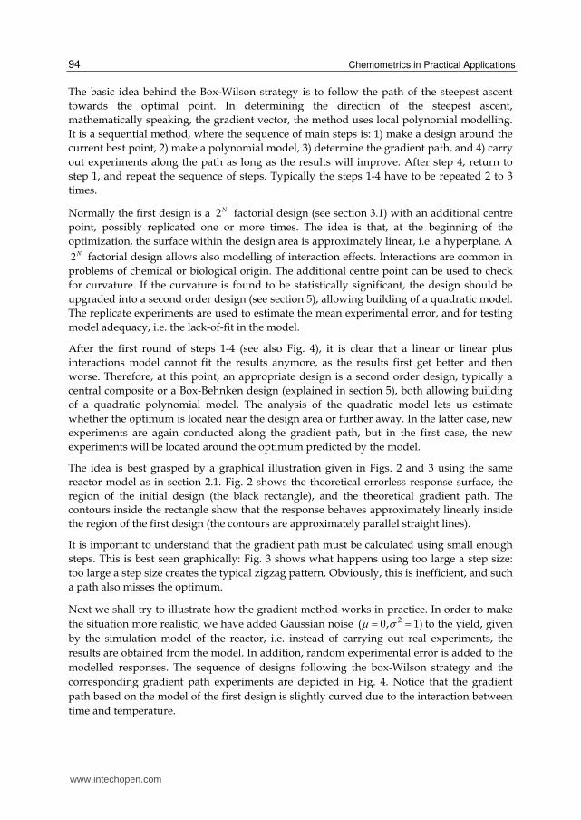
The idea is best grasped by a graphical illustration given in Figs. 2 and 3 using the same reactor model as in section 2.1. Fig. 2 shows the theoretical errorless response surface, the region of the initial design (the black rectangle), and the theoretical gradient path. The contours inside the rectangle show that the response behaves approximately linearly inside the region of the first design (the contours are approximately parallel straight lines).
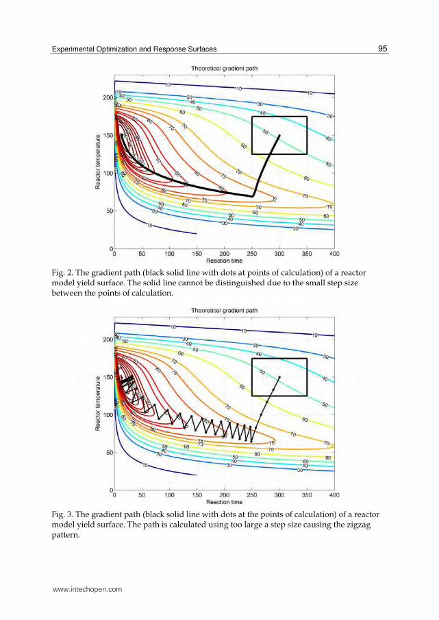
It is important to understand that the gradient path must be calculated using small enough
steps. This is best seen graphically: Fig. 3 shows what happens using too large a step size:
too large a step size creates the typical zigzag pattern. Obviously, this is inefficient, and such
a path also misses the optimum.
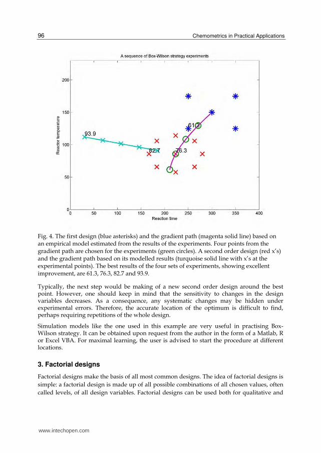
Next we shall try to illustrate how the gradient method works in practice. In order to make
the situation more realistic, we have added Gaussian noise 2( 0, 1) to the yield, given
by the simulation model of the reactor, i.e. instead of carrying out real experiments, the
results are obtained from the model. In addition, random experimental error is added to the
modelled responses. The sequence of designs following the box-Wilson strategy and the
corresponding gradient path experiments are depicted in Fig. 4. Notice that the gradient
path based on the model of the first design is slightly curved due to the interaction between
time and temperature.
www.intechopen.com
Experimental Optimization and Response Surfaces
95
Fig. 2. The gradient path (black solid line with dots at points of calculation) of a reactor model yield surface. The solid line cannot be distinguished due to the small step size between the points of calculation.
Fig. 3. The gradient path (black solid line with dots at the points of calculation) of a reactor model yield surface. The path is calculated using too large a step size causing the zigzag pattern.
www.intechopen.com
Chemometrics in Practical Applications
96
Fig. 4. The first design (blue asterisks) and the gradient path (magenta solid line) based on an empirical model estimated from the results of the experiments. Four points from the gradient path are chosen for the experiments (green circles). A second order design (red x’s) and the gradient path based on its modelled results (turquoise solid line with x’s at the experimental points). The best results of the four sets of experiments, showing excellent improvement, are 61.3, 76.3, 82.7 and 93.9.
Typically, the next step would be making of a new second order design around the best point. However, one should keep in mind that the sensitivity to changes in the design variables decreases. As a consequence, any systematic changes may be hidden under experimental errors. Therefore, the accurate location of the optimum is difficult to find, perhaps requiring repetitions of the whole design.
Simulation models like the one used in this example are very useful in practising Box-Wilson strategy. It can be obtained upon request from the author in the form of a Matlab, R or Excel VBA. For maximal learning, the user is advised to start the procedure at different locations.
3. Factorial designs
Factorial designs make the basis of all most common designs. The idea of factorial designs is
simple: a factorial design is made up of all possible combinations of all chosen values, often
called levels, of all design variables. Factorial designs can be used both for qualitative and
www.intechopen.com

Experimental Optimization and Response Surfaces
97
quantitative variables. If variables 1 2, , , Nx x x have 1 2, , , Nm m m different levels, the
number of experiments is 1 2 Nm m m . As a simple example, let us consider a case where
the variables and their levels are: 1x the type of a catalyst (A, B and C), 2x the catalyst
concentration (1 ppm and 2 ppm), and 3x the reaction temperature (60 ˚C, 70 ˚C and 80 ˚C).
The corresponding factorial design is given in Table 1.
x1 x2 x3
A 1 60
B 1 60
C 1 60
A 2 60
B 2 60
C 2 60
A 1 70
B 1 70
C 1 70
A 2 70
B 2 70
C 2 70
A 1 80
B 1 80
C 1 80
A 2 80
B 2 80
C 2 80
Table 1. A simple factorial design of three variables.
It is good to understand why factorial designs are good designs. The main reasons are that
they are orthogonal and balanced. Orthogonality means that the factor (variable) effects can be
estimated independently. For example, in the previous example the effect of the catalyst can
be estimated independently of the catalyst concentration effect. In a balanced design, each
variable combination appears equally many times. In order to understand why
orthogonality is important, let us study an example of a design that is not orthogonal. This
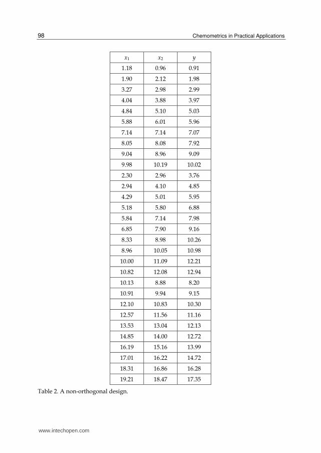
design, given in Table 2 below, has two design variables, 1x and 2x , and one response
variable, y.
www.intechopen.com
Chemometrics in Practical Applications
98
x1 x2 y
1.18 0.96 0.91
1.90 2.12 1.98
3.27 2.98 2.99
4.04 3.88 3.97
4.84 5.10 5.03
5.88 6.01 5.96
7.14 7.14 7.07
8.05 8.08 7.92
9.04 8.96 9.09
9.98 10.19 10.02
2.30 2.96 3.76
2.94 4.10 4.85
4.29 5.01 5.95
5.18 5.80 6.88
5.84 7.14 7.98
6.85 7.90 9.16
8.33 8.98 10.26
8.96 10.05 10.98
10.00 11.09 12.21
10.82 12.08 12.94
10.13 8.88 8.20
10.91 9.94 9.15
12.10 10.83 10.30
12.57 11.56 11.16
13.53 13.04 12.13
14.85 14.00 12.72
16.19 15.16 13.99
17.01 16.22 14.72
18.31 16.86 16.28
19.21 18.47 17.35
Table 2. A non-orthogonal design.
www.intechopen.com

Experimental Optimization and Response Surfaces
99
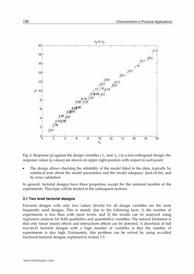
Now, if we plot the response against the design variables we get the following plot:
Fig. 5. Response (y) against the design variables ( 1x and 2x ) in a non-orthogonal design;
upper panel: y against, lower panel: y against.
Now, Fig. 5 clearly gives the illusion that the response depends approximately linearly both
on 1x and 2x with positive slopes. However, the true slope between y and 1x is negative.
To see this, let us plot the design variable against each other and show the response values
as text, as shown in Fig. 6.
Now, careful inspection of Fig. 6 reveals that actually yield decreases when increases. The
reason for the wrong illusion that Fig. 5 gives is that 1x and 2x are strongly correlated with
each other, i.e. the design variables are collinear. Although fitting a linear regression model
using both design variables would give correct signs for the regression coefficients,
collinearity will increase the confidence intervals of the regression coefficients. Problems of
this kind can be avoided by using factorial designs.
After this example, it is obvious that orthogonality, or near orthogonality, is a desired property of a good experimental design. Other desired properties are
The design contains as few experiments as possible for reliable results. The design gives reliable estimates for the empirical model fitted to the data.
www.intechopen.com
Chemometrics in Practical Applications
100
Fig. 6. Response (y) against the design variables ( 1x and 2x ) in a non-orthogonal design; the
response values (y values) are shown on upper right position with respect to each point.
The design allows checking the reliability of the model fitted to the data, typically by statistical tests about the model parameters and the model adequacy (lack-of-fit), and by cross validation.
In general, factorial designs have these properties, except for the minimal number of the experiments. This topic will be treated in the subsequent sections.
3.1 Two level factorial designs
Factorial designs with only two values (levels) for all design variables are the most frequently used designs. This is mainly due to the following facts: 1) the number of experiments is less than with more levels, and 2) the results can be analysed using regression analysis for both qualitative and quantitative variables. The natural limitation is that only linear (main) effects and interactions effects can be detected. A drawback of full two-level factorial designs with a high number of variables is that the number of experiments is also high. Fortunately, this problem can be solved by using so-called fractional factorial designs, explained in section 3.3.
www.intechopen.com

Experimental Optimization and Response Surfaces
101
Two-level factorial designs, usually called 2N designs, are typically tabulated using dimensionless coded variables having only values -1 or +1. For example, for a variable that represents a catalyst type, type A might correspond to -1 and type B might correspond to +1, or coarse raw material might be -1 and fine raw material might be +1. For quantitative variables, coding can be performed by the formula
12
i ii
i
x xX
x (1)
where iX stands for the coded value of the i’th variable, 1x stands for the original value of
the i’th variable, ix stands for the centre point value of the original i’th variable, and ix
stands for the difference of the original two values of the i’th variable. The half value of the
difference is called the step size. All statistical analyses of the results are usually carried out
using the coded variables. Quite often, we need to convert also coded dimensionless values
into the original physical values. For quantitative variables, we can simply use the inverse of
Eq. 1, i.e.
12
i i i ix x x X (2)
Tables of two-level factorial designs can be found in most textbooks of DOE. A good source is also NIST SEMATECH e-Handbook of Statistical Methods (NIST SEMATCH). Another way to create such tables is to use DOE-software e.g. (JMP, MODDE, MiniTab,…). It is also very easy to create tables of two-level factorial designs in any spreadsheet program. For example in Excel, you can simply enter the somewhat hideous formula
=2*MOD(FLOOR((ROW($B3)-ROW($B$3))/2^(COLUMN(C$2)-COLUMN($C$2));1);2)-1
into the cell C3, and then first copy the formula to the right as many time as there are
variables in the design (N) and finally copy the whole first row down 2N times. Of course, you can enter the formula anywhere in the spreadsheet, e.g. if you enter it into the cell D7 the references in the ROW functions must be changed into $C7 and $C$7, and the references in the column function must be changed into D$6 and $D$6, respectively.
If all variables are quantitative it is advisable to add a centre point into the design, i.e. an experiment where all variables are set to their mean values. Consequently, in coded units, all variables have value 0. The centre point experiment can be used to detect nonlinearities within the design area. If the mean experimental error is not known, usually the most
effective way to find it out is to repeat the centre point experiment. All experiments, including the possible centre point replicates, should be carried out in random order. The importance of randomization is well explained in e.g. (Box, Hunter & Hunter).
3.1.1 Empirical models related to two-level factorial designs
2N designs can be used only for linear models with optional interaction terms up order N.
By experience, it is known that interaction of order higher than two are seldom significant.
Therefore, it is common to consider those terms as random noise, giving extra degrees of
freedom for error estimation. However, one should be careful about such interpretations,
www.intechopen.com

Chemometrics in Practical Applications
102
and models should always be carefully validated. It should also be noted that the residual
errors always contain both experimental error and modelling error. For this reason,
independent replicate experiments are of utmost importance, and only having a reliable
estimate of the experimental error gives a possibility to check for lack-of-fit, i.e. the model
adequacy.
The general form of a model for a response variable y with linear terms and interaction terms up to order N is
1
N N N
i i ij i j ijk i j ki i j i j k
y b X b X X b X X X (3)
The number of terms in the second sum is 2
N
, and in the third sum it is3
N
, and so on.
The most common model types used are models with linear terms only, or models with linear terms and pairwise interaction terms.
If all terms of model (3) are used, and there are no replicate experiments in the
corresponding 2N design, there are as many unknown parameters in the model as there are
experiments in the design, leaving no degrees of freedom for the residual error, i.e. all
residuals are zero. In such cases, the design is called saturated with respect to the model, or
just saturated, if it is obvious what the model is. In these cases traditional statistical tests
cannot be employed. Instead, the significant terms can often be detected by inspecting the
estimated model parameter values using normal probability plots.
Later we need to differentiate between the terms “design matrix” and “model matrix”. A
design matrix is a expN N matrix whose columns are the values of design variables where
expN is the number of experiments. A model matrix is a expN p matrix that is the design
matrix appended with columns corresponding to the model terms. For example, a model
matrix for a linear plus interaction model for two variables has a column of ones
(corresponding to the intercept), columns for values of 1X and 2X and a column for values
of the product 1 2X X .
It is good to understand the nature of the pairwise interaction terms. Let us consider a
model for two variables, i.e. 0 1 1 2 2 12 1 2 y b b X b X b X X , and let us rearrange the terms as 0 1 1 2 12 1 2 y b b X b b X X . This form reveals that the interaction actually means that the
slope of 2X depends linearly on 1X . Taking 1X as the common factor instead of 2X shows
that the slope of 1X depends linearly on 2X . In other words, a pairwise interaction between
two variables means that the other variable affects the effect of the other one. If two
variables don’t interact, their effects are said to be additive. Fig. 7 depicts additive and
interacting variables.
In problems of chemical or biological nature, it is more a rule than an exception that
interactions between variables exist. Therefore, main effect models serve only as rough
approximations, and are used typically in cases with a very high number of variables. It is
also quite often useful to try to model some transformation of the response variable,
www.intechopen.com

Experimental Optimization and Response Surfaces
103
Fig. 7. Linear dependency of y on 1x and on 2x . Left panel: an additive case without
interaction, right panel: a non-additive case. Blue line: 2x has a constant value, green line:
2x has another constant value.
typically a logarithm, or a Box-Cox transformation. Usually the aim is to find a transformation that makes the residuals as normal as possible.
3.1.2 Analysing the results of two level factorial designs
Two level factorial designs can be analysed either by analysis of variance (ANOVA) or by
regression analysis. Using regression analysis is more straightforward, and we shall
concentrate on it in the sequel. However, one should bear in mind that the interpretation of the
estimated model parameter is different between quantitative and qualitative variables.
Actually, due to the orthogonality of 2N designs, regression analysis could be carried out
quite easily even by hand using the well-known Yates algorithm, see e.g. (Box & Draper, 2007).
Ordinary least squares regression (OLS) is the most common way to analyse results of orthogonal designs, but sometimes more robust techniques, e.g. minimizing the median of absolute values of the residuals, can be employed. Using latent variable techniques, e.g. PLS, doesn’t give any extra benefit with orthogonal designs. However, in some other kind of designs, typically optimal designs or mixture designs, latent variable techniques can be useful.
www.intechopen.com
Chemometrics in Practical Applications
104
The mathematics and statistical theory behind regression analysis can be found in any basic textbook about regression analysis or statistical linear models see e.g. (Weisberg, 1985) or (Neter et. al., 1996). In this chapter we shall concentrate on applying and interpreting the results of OLS in DOE problems. However, it is always good to bear in mind the statistical assumptions behind the classical regression tests, i.e. approximately normally distributed and independent errors. The latter is more important, and dependencies between random errors can make the results of the tests completely useless. This fact is well illustrated in (Box et. al., 2005). Even moderate deviations from normality are usually not too harmful, unless they are caused by gross errors, i.e. by outliers. For this reason, normal probability plots, or other tools for detecting outliers, should always be included in validating the model.
Since OLS is such a standard technique, a plethora of software alternatives exists for carrying out the regression analyses of the results of a given design. One can use general mathematics software like Matlab, Octave, Mathematica, Maple etc., or general purpose statistical software like S-plus, R, Statistica, MiniTab, SPSS, etc, or even spreadsheet programs like Excel or Open Office Calc. However, it is advisable to use software that contains those model validation tools that are commonly used with designed experiments. Practically all general mathematical or statistical software packages contain such tools.
Quite often there are more than one response variables. In such cases, it is typical to estimate models for each response separately. If a multivariate response is a ‘curve’, e.g. a spectrum or a distribution, it may be simpler to use latent variable methods, typically PLS or PCR.
This example is taken from Box & Draper (Box & Draper, 2007).
3.2 Model validation
Model validation is an essential part of analysing the results of a design. It should be noted that most of the techniques presented in this section can be used with all kinds of designs,
not only with 2N designs.
In the worst case, the validation yields the conclusion that the design variables have no effect on the response(s), significantly different from random variation. In such a case, one has to consider the following alternatives: 1) to increase the step sizes in the design variables, 2) to replicate the experiments one or more times, or 3) to make a new design with new design variables. In the opposite case, i.e. the model and at least some of the design variables are found to be statistically significant, the continuation depends on the scope of the design, and on the results of the (regression) analysis. The techniques used for optimization tasks are presented in subsequent sections.
3.2.1 Classical statistical tests
Classical statistical tests can be applied mainly to validate regression models that are linear with respect to the model parameters. The most common empirical models used in DOE are linear models (main effect models), linear plus interactions models, and quadratic models. They all are linear with respect to the parameters. The most useful of these (in DOE context) are 1) t-tests for testing the significance of the individual terms of the model, 2) the lack-of-fit test for testing the model adequacy, and 3) outlier tests based on so-called externally studentized residuals, see e.g. (Neter et. al., 1996).
www.intechopen.com

Experimental Optimization and Response Surfaces
105
The t-test for testing the significance of the individual terms of the model is based on the test
statistic that is calculated by dividing a regression coefficient by its standard deviation. This
statistic can be shown to follow the t-distribution with 1 n p degrees of freedom where n
is the number experiments, and p is the number of model parameters. If the model doesn’t
contain an intercept, the number of degrees of freedom is n p . Typically, a term in the
model is considered significant if the p-value of the test statistic is below 0.05.
The standard errors of the coefficients are usually based on the residual error. If the design
contains a reasonable number of replicates this estimate can also be based on the standard
error of the replicates. The residual based standard error of the i’th regression coefficient ibs
can be easily transformed into replicate error based ones by the formula /iE R bMS MS s . In
this case the degrees of freedom are 1rn (the symbols are explained in the next
paragraph).
The lack-of fit test can be applied only if the design contains replicate experiments which
permit estimation of the so-called pure error, i.e. an error term that is free from modelling
errors. Assuming that the replicate experiments are included in regression, the calculations
are carried out according to the following equations. First calculate the pure error sum of
squares ESS
2
1
,
rn
E ii
SS y y (4)
where rn is the number of replicates, iy ’s are outcomes of the replicate experiments, and y
is the mean value of the replicate experiments. The number of degrees of freedom of ESS is
1rn . Then calculate the residual sum of squares RSS :
21
ˆ ,
nR ii
SS y y (5)
where n is the number of experiments and y ’s are the fitted values, i.e. the values
calculated using the estimated model. The number of degrees of freedom of RSS is
1 n p , or n p if the model doesn’t contain an intercept. Then calculate the lack-of-fit
sum of squares LOFSS :
LOF R ESS SS SS (6)
The number of degrees of freedom of LOFSS is 1 rn n p , or rn n p if the model
doesn’t contain an intercept. Then, calculate the lack-of-fit mean squares LOFMS and the
pure error mean squares EMS by dividing the corresponding sums of squares by their
degrees of freedom. Finally, calculate the lack-of-fit test statistic /LOF LOF EF MS MS . It can
be shown that LOFF follows an F-distribution with 1 rn n p (or rn n p ) and 1rn
degrees of freedom. If LOFF is significantly greater than 1, it is said that the model suffers
from lack-of-fit, and if it is significantly less than 1, it is said that the model suffers from
over-fit.
www.intechopen.com

Chemometrics in Practical Applications
106
An externally studentized residual is a deleted residual, i.e. residual calculated using leave-
one-out cross-validation, divided the standard error of deleted residuals. It can be shown
that the externally studentized residuals follow a t-distribution with 2 n p degrees of
freedom, or 1 n p degrees of freedom if the model doesn’t contain an intercept. If the p-
value of an externally studentized residual is small enough, the result of the corresponding
experiment is called an outlier. Typically, outliers should be removed, or the corresponding
experiments should be repeated. If the result of a repeated experiment still gives an outlying
value, it is likely that model suffers from lack-of-fit. Otherwise, the conclusion is that
something went wrong in the original experiment.
3.2.2 Cross-validation
Cross-validation is familiar to all chemometricians. However, in using cross-validation
for validating results of designed experiments some important issues should be
considered. First, cross-validation requires extra degrees of freedom, and consequently
all candidate models cannot be cross-validated. For example, in a 22 design, a model
containing linear terms and the pairwise interaction cannot be cross-validated.
Secondly, often the designs become severely unbalanced, when observations are left
out. For example, in a 22 design with a centre point, the model containing linear terms
and the pairwise interaction can be cross-validated, but when the corner point (+1, +1)
is left out, the design is very weak for estimating the interaction term; in such cases the
results of cross-validation can be too pessimistic. On the other hand, replicated
experiments may give too optimistic results in cross-validation, as the design variable
combinations corresponding to replicate experiments are never left out. This problem
can be easily avoided by using the response averages instead of individual responses of
the replicated experiments.
Usually only statistically significant terms are kept in the final model. However, it is also
common to include mildly non-significant terms in the model, if keeping such terms
improves cross-validated results.
3.2.3 Normal probability plots
Normal probability plots, also called normal qq-plots, can be used to study either the
regression coefficients or the residuals (or deleted residuals). The former is typically used in
saturated models where ordinary t-tests cannot be applied. Normal probability plots are
constructed by first sorting the values from the smallest to largest. Then the proportions 0.5 / ip i n are calculated, where n is the number of the values, and i is the ordinal
number of a sorted value, i.e. 1 for the smallest value and n for the largest value (subtracting
0.5 is called the continuity correction). Then the normal score, i.e. inverse of ip using the
standard normal distribution, is calculated. Finally, the values are plotted against the
normal scores. If the distribution of the values is normal, the points lie approximately on a
straight line. The interpretation in the former case is that the leftmost or the rightmost values
that do not follow a linear pattern represent significant terms. In the latter case, the same
kind of values represent outlying residuals.
www.intechopen.com

Experimental Optimization and Response Surfaces
107
3.2.4 Variable selection
If the design is orthogonal, or nearly orthogonal, removing or adding terms into the model doesn’t affect the significance of the other terms. This is also the case if the estimates of the standard error of the coefficients are based on the standard error of the estimates (cf. 3.2.1).
Therefore, variable selection based on significance is very simple; just take the variables significant enough, without worrying about e.g. the order of taking terms into a model. Because models based on designed experiments are often used for extrapolatory prediction, one should, whenever possible, test the models using cross-validation. However, one should bear in mind the limitations of cross-validation when it is applied to designed experiments
(cf. 3.2.2). In addition, it is wise also to test models with almost significant variables using cross-validation, since sometimes such models have better predictive power.
If the design is not orthogonal, traditional variable (feature) selection techniques can be used, e.g. forward, backward, stepwise, or all checking possible models (total search). Naturally, the selection can be based on different criteria, e.g. Mallows pC , PRESS, 2R , 2Q , Akaike’s information etc., see e.g. (Weisberg, 1985). If models are used for extrapolatory prediction, a good choice for a criterion is to minimize PRESS or maximize 2Q . In many cases of DOE modelling, the number of possible model terms, typically linear, pair-wise interaction, and quadratic terms, is moderate. For example, a full quadratic model for 4 variables has 14 terms, plus the intercept. Thus the number of all possible sub-models is 214 which is 16384. In such cases, with the speed of modern computers, it is easy to test all sub-models with respect to the chosen criterion. However, if the number of variables is greater, going through all possible regression models becomes impossible in practice. In such cases, one can use genetic algorithms, see e.g. (Koljonen & al., 2008).
Another approach is to use latent variable techniques, e.g. PLS or PCR, in which the selection of the dimension replaces the selection of variables. Although variable selection seems more natural, and is more commonly used in typical applications of DOE than latent variable methods, neither of the approaches have been proved generally better. Therefore, it is good to try out different approaches, combined with proper model validation techniques.
A third alternative is to use shrinkage methods, i.e. different forms of ridge regression. Recently, new algorithms based on L1 norm have been developed, including such as LASSO (Tibshirani, 1996), LARS (Efron & al., 2004), or elastic nets (Zou & al., 2005). Elastic nets use combinations of L1 and L2 norm penalties. Penalizing the least squares solution by the L1 norm of the regression coefficient tends to make the non-significant terms zero which effectively means selecting variables.
In a typical application of DOE, the responses are multivariate in a way that they represent individual features which, in turn, typically depend on different variable combinations of the design variables. In such cases, it is better to build separate models for each response, i.e. the significant variables have to be selected separately for each response. However, if the response is a spectrum, or an object of similar nature, variable selection should usually be carried out for all responses simultaneously, using e.g. PLS regression or some other multivariate regression technique. In such cases, there’s an extra problem of combining the individual criteria of the goodness of fit into a single criterion. In many cases, a weighted average of e.g. the RMSEP values, i.e. the standard residual errors in cross-validation, of the individual responses is a good choice, e.g. using signal to noise ratios as weights.
www.intechopen.com

Chemometrics in Practical Applications
108
3.2.5 An example of a 2N design
As a simple example of a 2N design we take a 22 design published in the Brazilian Journal of Chemical Engineering (Silva et. al., 2011). In this study the ethanol production by Pichia stipitis was evaluated in a stirred tank bioreactor using semi defined medium containing xylose (90.0 g/l) as the main carbon source. Experimental assays were performed according to a 22 full factorial design to evaluate the influence of aeration (0.25 to 0.75 vvm) and agitation (150 to 250 rpm) conditions on ethanol production. The design contains also a centre point (0.50 vvm and 200 rpm), and in a replication of the (+1, +1) experiment. It should be noted that this design is not fully orthogonal due the exceptional selection of the replication experiment (the design would have been orthogonal, if the centre point had been replicated).
The results of the design are given in Table 3 below (X1 and X2 refer to aeration and agitation in coded levels, respectively).
Assay Aeration Agitation X1 X2 Production (g/l)
1 0.25 150 -1 -1 23.0
2 0.75 150 1 -1 17.7
3 0.25 250 -1 1 26.7
4 0.75 250 1 1 16.2
5 0.75 250 1 1 16.1
6 0.50 200 0 0 19.4
Table 3. A 22 design.
Fig. 8 shows the effect of aeration at the two levels of agitation. From the figure, it is clear that aeration has much greater influence on productivity (Production) than agitation. It also shows an interaction between the variables. Considering the very small difference in the response between the two replicate experiments, it is plausible to consider both aeration and the interaction between aeration and agitation significant effects.
Fig. 8. Production vs. aeration. Blue solid line: Agitation = 150; red dashed line: Agitation = 250.
www.intechopen.com

Experimental Optimization and Response Surfaces
109
If we carry out classical statistical tests used in regression analysis, it should be remembered that the design has only one replicated experiment, and consequently very few degrees of freedom for the residual error. Testing lack-of-fit, or nonlinearity, is also unreliable because we can estimate the (pure) experimental error with only one degree of freedom. However, it is always possible to use common sense and investigations about the effects on relative basis. For example, the difference between the centre point result and the mean value of the other (corner point) results is only 0.45 which is relatively small compared to differences between the corner points. Therefore, it is highly unlikely that the behaviour would be nonlinear within the experimental region. Consequently, it is likely that the model doesn’t suffer from lack-of-fit, and a linear plus interaction model should suffice.
Now, let us look at the results of the regression analyses of a linear plus interaction model (model 1), the same model without the agitation main effect (model 2), and the model with aeration only (model 3). The regression analyses are carried out using basic R and some additional DOE functions written by the author (these DOE functions, including the R-scripts of all examples of this chapter, are available from the author upon request).
The R listing of the summary of the regression models 1, 2 and 3 are given in Tables 4-6 below. Note that values of the regression coefficients of the same effects vary a little between the models. This is due to the fact that design is not fully orthogonal. In an orthogonal design, the estimates of the same regression coefficients will not change when terms are dropped out.
Estimate Std. Error t value p value
(Intercept) 20.6205 0.4042 51.015 0.000384 X1 -3.9244 0.4454 -8.811 0.012638
X2 0.5756 0.4454 1.292 0.325404
I(X1 * X2) -1.2744 0.4454 -2.861 0.325404
Residual standard error: 0.9541 on 2 degrees of freedom Multiple R-squared: 0.9796, Adjusted R-squared: 0.9489 F-statistic: 31.95 on 3 and 2 DF, p-value: 0.03051
Table 4. Regression summary of model 1 (I(X1 * X2) denotes interaction between X1 and X2).
Estimate Std. Error t value p value
(Intercept) 20.6882 0.4433 46.668 2.17e-05 X1 -3.8397 0.4873 -7.879 0.00426
I(X1 * X2) -1.1897 0.4873 -2.441 0.09238
Residual standard error: 1.055 on 3 degrees of freedom Multiple R-squared: 0.9625, Adjusted R-squared: 0.9375 F-statistic: 38.48 on 2 and 3 DF, p-value: 0.007266
Table 5. Regression summary of model 2 (I(X1 * X2) denotes interaction between X1 and X2).
www.intechopen.com

Chemometrics in Practical Applications
110
Estimate Std. Error t value p value
(Intercept) 20.5241 0.6558 31.3 6.21e-06 X1 -4.0448 0.7184 -5.63 0.0049
Residual standard error: 1.579 on 4 degrees of freedom Multiple R-squared: 0.8879, Adjusted R-squared: 0.8599 F-statistic: 38.48 on 1 and 4 DF, p-value: 0.004896
Table 6. Regression summary of model 3.
The residual standard error is approximately 1 g/l in models 1 and 2. This seems quite high compared to the variation in replicate experiments (16.2 and 16.1 g/l) corresponding to the pure experimental pure error standard deviation of ca. 0.071 g/l. The calculations of a lack-of-fit test for model 2 are the following: The residual sum of squares (SSRES) is 3·1.0552 = 3.339. The pure error sum of squares (SSE) is 1·0.0712 = 0.005. The lack-of-fit sum of squares (SSLOF) is 3.339-0.005 = 3.334. The corresponding mean squares are SSLOF/( dfRES- dfE) = SSLOF/(3-1) = 3.334/2 = 1.667 and the lack-of-fit F-statistic is MSLOF/MSE = 1.667/0.005 = 333.4 having 2 and 1 degrees of freedom. The corresponding p-value is 0.039 which is significant at the 0.05 level of significance. Thus, a formal lack-of-fit test exhibits significant lack-of-fit, but one must keep in mind that estimating standard deviation from only two observations is very unreliable. The lack-of-fit p-values for models 1 and 3 are 0.033 and 0.028, respectively, i.e. the lack-of-fit is least significant in model 2.
The effect of aeration (X1) is significant in all models, and according to model 1 it is obvious that agitation doesn’t have a significant effect on productivity. The interaction term is not significant in any of the models; however, it is not uncommon to include terms whose p-values are between 0.05 and 0.10 in models used for designing new experiments. The results of the new experiments would then either support or contradict the existence of an interaction.
Carrying out the leave-one-out (loo) cross-validation, gives the following Q2 values (Table 7).
Model R2 Q2
1 98.0 -22.0
2 96.2 84.5
3 88.8 68.1
Table 7. Comparison of R2 and Q2 values between model 1-3.
Fig. 9 shows the fitted and CV-predicted production values and the corresponding residual normal probability plots of models 1-3. By cross-validation, the model 2, i.e.
0 1 1 12 1 2 y b b X b X X , is the best one. Finally, Fig. 10 shows the contour plot of the best
model, model 2.
www.intechopen.com

Experimental Optimization and Response Surfaces
111
Fig. 9. Cross-validation of models 1-3. Left panel: Production vs. the number of experiment; black circles: data; blue triangles: fitted values; red pluses: cross-validated leave-one-out prediction. Right panel: Normal probability plots of the cross-validated leave-one-out residuals.
www.intechopen.com

Chemometrics in Practical Applications
112
Fig. 10. Production vs. Aeration and Agitation.
3.3 Fractional 2N designs (2
N-p designs)
The number of experiments in 2N designs grows rapidly with the number of variables N. This problem can be avoided by choosing only part of the experiments of the full design. Naturally, using only a fraction of the full design, information is lost. The idea behind fractional 2N designs is to select the experiments in a way that the information lost is related only to higher order interactions which seldom represent significant effects.
3.3.1 Generating 2N-p
designs
The selection of experiments in 2N-p designs can be accomplished by using so-called generators (see e.g. Box & al., 2005). A generator is an equation between algebraic elements
www.intechopen.com

Experimental Optimization and Response Surfaces
113
that represent variable effects, typically denoted by bold face numbers or upper case letters. For example 1 denotes the effect of variable 1. If there are more than 9 variables in the design, brackets are used to avoid confusion, i.e. we would use (12) instead of 12 to represent the effect of the variable 12. The bold face letter I represents the average response, i.e. the intercept of the model when coded variables are used. The generator elements (effects) follow the following algebraic rules of ‘products’ between the effects.
The effects are commutative, e.g. 12 = 21 The effects are associative, e.g. (12)3 = 1(23) I is a neutral element, e.g. I2 = 2 Even powers produce the neutral element, e.g. 22 = I or 2222 = I (naturally, for example 222 = 2)
Now, a generator of a design is an equation between a product of effects and I, for example
123 = I. The interpretation of a product, also called a word, is that of a corresponding
interaction between the effects. Thus, for example, 123 = I means that the third order
interaction between variables 1-3 is confounded with the mean response in a design
generated using this generator. Confounding (sometimes called aliasing) means that the
confounding effects cannot be estimated unequivocally using this design. For example, in a
design generated by 123 = I the model cannot contain both an intercept and a third order
interaction. If the model is deliberately chosen to have both an intercept and the third order
interaction term, there is no way to tell whether the estimate of the intercept really
represents the intercept or the third order interaction.
Furthermore, any equation derived from the original generator, using the given algebraic
rules, gives a confounding pattern. For example multiplying both sides of 123 = I by 1 gives
1123 = 1I. Using the given rules this simplifies into I23 = 1I and then into 23 = 1. Thus, in a
design with this generator the pairwise interaction between variable 2 and 3 is confounded
with variable 1. Multiplying the original generator by 2 and 3 it is easy to see that all
pairwise interactions are confounded with main effects (2 with 13 and 3 with 12) in this
design. Consequently, the only reasonable model whose parameters can be estimated
unequivocally, is the main effect model 0 1 1 2 2 3 3 y b b X b X b X . Technically possible
alternative models, but hardly useful in practice, would be e.g.
0 1 1 2 2 12 1 2 y b b X b X b X X or 123 1 2 3 1 1 2 2 3 3 y b X X X b X b X b X .
A design can be generated using more than one generator. Each generator halves the
number of experiments. For example, a design with two generators has only ¼ of the
original number of experiments in the corresponding full 2N design. If p is the number of
generators, the corresponding fractional 2N design is denoted by 2N-p.
In practice, 2N-p designs are constructed by first making a full 2N design table and then
adding columns that contain the interaction terms corresponding to the generator words.
Then only those experiments (rows) are selected where all interaction terms are +1.
Alternatively one can choose the experiments where all interaction terms are -1. As an
example, let us construct a 23-1 design with the generator 123 = I. The full design table
with an additional column containing the three-way interaction term is given in
Table 8.
www.intechopen.com

Chemometrics in Practical Applications
114
1x 2x 3x 1 2 3x x x
-1 -1 -1 -1
-1 -1 +1 +1
-1 +1 -1 +1 -1 +1 +1 -1
+1 -1 -1 +1
+1 -1 +1 -1
+1 +1 -1 -1 +1 +1 +1 +1
Table 8. A table for constructing a 23-1 design.
Now, the desired design table is obtained by deleting the rows 1, 4, 6 and 7. An alternative design is obtained by deleting the rows 2, 3, 5 and 8.
3.3.2 Confounding (aliasing) and resolution
An important concept related to 2N-p designs is the resolution of a design, denoted by roman
numerals. Technically, resolution is the minimum word length of all possible generators
derived from the original set of generators. For design with a single generator, finding out
the resolution is easy. For example, the resolution of the 23-1 design with the generator 123 =
I is III because the length of the word 123 is 3 (note that e.g. (12) would be counted as a
single letter in a generator word). If there are more generators than one, the situation is
more complicated. For example, if the generators in a 25-2 design were 1234 = I and 1235 = I,
then the equation 1234 = 1235 would be true which after multiplying both sides 1235 gives
45 = I. Thus the resolution of this design would be II. Naturally, this would be a really bad
design with confounding main effects.
The interpretation of the resolution of a design is (designs of resolution below III are
normally not used)
If the resolution is III, only a main effect model can be used If the resolution is IV, a main effect model with half of all the pairwise interaction
effects can be used If the resolution is V or higher, a main effect model with all pairwise interaction effects
can be used
If the resolution is higher than V also at least some of the higher order interaction can be estimated. There are many sources of tables listing 2N-p designs and their confounding patterns, e.g. Table 3.17 in (NIST SEMATCH). Usually these tables give so-called minimum aberration designs, i.e. designs that minimize the number of short words in all possible generators of a design with given N and p.
3.3.3 Example
This example is taken from (Box & Draper, 2007) (Example 5.2 p. 189), but the analysis is not completely identical to the one given in the book.
www.intechopen.com

Experimental Optimization and Response Surfaces
115
The task was to improve the yield (y) (in percentage) of a laboratory scale drug synthesis. The five design variables were the reaction time (t), the reactor temperature (T), the amount of reagent B (B), the amount of reagent C (C), and the amount of reagent D (D). The chosen design levels in a two level fractional factorial design are given in Table 9 below.
Coded Original Lower (-1) Upper (+1) Formula
X1 t 6 h 10 h 1
8
2
tX
X2 T 85⁰C 90⁰C 2
87.5
2.5
TX
X3 B 30 ml 60 ml 3
45
15
BX
X4 C 90 ml 115 ml 4
102.5
12.5
CX
X5 D 40 g 50 g 5
45
5
DX
Table 9. The variable levels of example 3.3.3.
The design was chosen to be a fractional resolution V design (25-1) with the generator I = 12345. The design table in coded units, including the yields and the run order of the experiments is given in Table 10 ( y stands for the yield).
order X1 X2 X3 X4 X5 y
16 -1 -1 -1 -1 1 51.8
2 1 -1 -1 -1 -1 56.3
10 -1 1 -1 -1 -1 56.8
1 1 1 -1 -1 1 48.3
14 -1 -1 1 -1 -1 62.3
8 1 -1 1 -1 1 49.8
9 -1 1 1 -1 1 49.0
7 1 1 1 -1 -1 46.0
4 -1 -1 -1 1 -1 72.6
15 1 -1 -1 1 1 49.5
13 -1 1 -1 1 1 56.8
3 1 1 -1 1 -1 63.1
12 -1 -1 1 1 1 64.6
6 1 -1 1 1 -1 67.8
5 -1 1 1 1 -1 70.3
11 1 1 1 1 1 49.8
Table 10. The design of example 3.3.3 in coded units.
Since the resolution of this design is V, we can estimate a model containing linear and pair-
wise interaction effects. However the design is saturated with respect to this model, and
www.intechopen.com

Chemometrics in Practical Applications
116
thus the model cannot be validated by statistical tests, or by cross-validation. The regression
summary is given Table 11.
Estimate Std. Error t value p value (Intercept) 57.1750 NA NA NA
t -3.3500 NA NA NA
T -2.1625 NA NA NA
B 0.2750 NA NA NA C 4.6375 NA NA NA
D -4.7250 NA NA NA
I(t * T) 0.1375 NA NA NA I(t * B) -0.7500 NA NA NA
I(T * B) -1.5125 NA NA NA
I(t * C) -0.9125 NA NA NA
I(T * C) 0.3500 NA NA NA I(B * C) 1.0375 NA NA NA
I(t * D) 0.2500 NA NA NA
I(T * D) 0.6875 NA NA NA
I(B * D) 0.5750 NA NA NA I(C * D) -1.9125 NA NA NA
Residual standard error: NaN on 0 degrees of freedom Multiple R-squared: 1, Adjusted R-squared: NaN F-statistic: NaN on 15 and 0 DF, p-value: NA
Table 11. Regression summary of the linear plus pairwise interactions model. NA stands for “not available”.
Because the design is saturated with respect to the linear plus pairwise interactions model there are no degrees of freedom for any regression statistics. Therefore, for selecting the significant terms we have to use either a normal probability plot of the estimated values of the regression coefficient or variable selection techniques. We chose to use forward selection based on the Q2 value. This technique gave the maximum Q2 value in a model with 4 linear terms and 7 pairwise interaction terms. However, after 6 terms the increase in the Q2 value is minimal, and in order to avoid over-fitting we chose to use the model with 6 terms. The chosen terms were the main effects of t, T, C and D, and the interaction effects between C and D and between T and B. This model has a Q2 value 83.8 % and the regression summary for this model is given in Table 12.
All terms in the model are now statistically significant at 5 % significance level, and the predictive power of the model is fairly good according the Q2 value . Section 4.3 shows how this model has been used in search for improvement.
3.4 Plackett-Burman (screening) designs
If the number of variables is high, and the aim is to select the most important variables for further experimentation, usually only the main effects are of interest. In such cases the most cost effective choice is to use designs that have as many experiments as there are parameters in
www.intechopen.com

Experimental Optimization and Response Surfaces
117
Estimate Std. Error t value p value
(Intercept) 57.1750 0.6284 90.980 1.19e-14 t -3.3500 0.6284 -5.331 0.000474
T -2.1625 0.6284 -3.441 0.007378
C 4.6375 0.6284 7.379 4.19e-05
D -4.7250 0.6284 -7.519 3.62e-05 I(T * B) -1.5125 0.6284 -2.407 0.039457
I(C * D) 1.9125 0.6284 -3.043 0.013944
Residual standard error: NaN on 0 degrees of freedom Multiple R-squared: 1, Adjusted R-squared: NaN
F-statistic: NaN on 15 and 0 DF, p-value: NA
Table 12. Regression summary of the 6 terms model.
the corresponding main effect model, i.e. N+1 experiments. It can be proved that such designs that are also orthogonal exist in multiples of 4, i.e. for 3, 7, 11, … variables having 4, 8, 12, … experiments respectively. The ones in which the number of experiments is a power of 2 are actually 2N-p designs. Thus for example a Plackett-Burman design for 3 variables that has 8 = 23 experiments is a 23-1 design. General construction of Plackett-Burman designs is beyond the scope of this chapter. The interested reader can refer to e.g. section 5.3.3.5 in (NIST SEMATECH). Plackett-Burman designs are also called 2-level Taguchi designs or Hadamard matrices.
3.5 Blocking
Sometimes uncontrolled factors, such as work shifts, raw material batches, differences in pieces of equipment, etc., may affect the results. In such cases the effects of such variables should be taken into account in the design. If the design variables are qualitative, such classical designs as randomized blocks design, Latin square design, or Graeco-Latin square design can be used, see e.g. (Montgomery, 1991). If the design variables are quantitative, a common technique is to have extra columns (variables) for the uncontrolled variables. For 2N and CC-designs, tables of different blocking schemes exist, see e.g. section 5.3.3.3.3. in (NIST SEMATECH).
3.6 Sizing designs
An important issue in DOE is the total number of experiments, i.e. the size of a design.
Sizing can be based on predictive power, or on the power of detecting differences of
predefined size Δ. The latter is more commonly used, and many commercial DOE software
packages have tools for determining the required number of estimates in such a way that
the statistical power, i.e. 1 ( is the probability of type II error), has a desired value at a
given level of significance . For pairwise comparisons, exact methods based on the non-
central t-distribution exist. For example, in R the function called power.t.test can be used to
find the number of experiments needed in pairwise comparisons. For multiple comparisons,
one can use the so-called Wheeler’s formula (Wheeler, 1974) for an estimate of the required
number of experiments n: 24 / n r where r is the number of levels of a factor, is the
experimental standard deviation, and is size of the difference. The formula assumes that
www.intechopen.com
Chemometrics in Practical Applications
118
the level of significance is 0.05, and the power 1 is 0.90. Wheeler gives also formulas
for several other common design/model combinations (Wheeler, 1974).
4. Improving results by steepest ascent
If the goal of the experimentation has been to optimize something, the next step after
analysing the results of a 2N or a fractional 2N design is to try to make improvement using
knowledge provided by the analysis. The most common technique is the method of steepest
ascent, also called the gradient (path) method.
4.1 Calculating the gradient path
It is well known from calculus that the direction of the steepest ascent on a response surface
is given by the gradient vector, i.e. the vector of partial derivatives with respect to the design
variables at a given point. The basic idea has been presented in section 3.2, and now we shall
present the technical details.
In principle, the procedure is simple. First we choose a starting point, say 0X , which
typically is the centre point of the design. Then we calculate the gradient vector, say at
this point. Note that it is important to use coded variables in gradient calculations. Next, the
gradient vector has to be scaled small enough in order to avoid zigzagging (see 2.2). This can
be done by multiplying the corresponding unit vector, 0 / , by a scaling factor, say
c. Now, the gradient path points are obtained by calculating , 1,2, , 0X = X + i (i-1) c i n
where n is the number of points. Once the points have been calculated, the experimental
points are chosen from the path so that the distance between the points matches the desired
step size, typically 1 in coded units. Naturally, the coded values have to be decoded into
physical values having the original units before experimentation.
4.2 Alternative improvement techniques
Another principle in searching optimal new experiments is to use direct optimization
techniques using the current model. In this approach, first the search region has to be
defined. There are basically two different alternatives: 1) a hypercube whose centre is at the
design centre with a given length for the sides of the hypercube, or 2) a hypersphere whose
centre is at the design centre with a given radius. In the first alternative, typically the length
of the side is first set to a value slightly over 2, say 3, giving mild extrapolation outside the
experimental region. In the latter, typically the length of the radius is first set to a value
slightly over 1, say 1.5, giving mild extrapolation outside the experimental region.
If the model is a linear plus pair-wise interactions model, the solution can easily be shown to
be one of the vertices of the hypercube in the hypercube approach. If the model is a
quadratic one, and the optimum (according to the model) is not inside the hypercube, the
solution is a point on one of the edges of the hypercube and a point on the hypersphere in
the hypersphere approach. In both approaches, the solution is found most easily using some
iterative constrained optimization tool, e.g. Excel’s Solver Tool. In the latter (hypersphere)
approach, it is easy to show, using the Lagrange multiplier technique of constrained
www.intechopen.com

Experimental Optimization and Response Surfaces
119
optimization, that the optimal point Xopt on the hypersphere of radius r is obtained by 12
X B I bopt , where is solved from the equation 1 2 22 B I b r . The notation is
explained in section 5.2. Unfortunately, must be solved numerically unless the model is
linear. The benefit of using (numerical) iterative optimization in both approaches, or using
the gradient path technique, is that they all work for all kind of models, not only for
quadratic ones.
4.3 Example
Let us continue with the example of section 3.3.3 and see how the model can be used to design new experiments along the gradient path. The model of the previous example can be written (in coded variables)
0 1 1 2 2 4 4 5 5 23 2 3 45 4 5 y b b X b X b X b X b X X b X X (7)
The coefficients (b’s) refer to the values given in Table 12. The gradient, i.e. the direction of steepest ascent, is the vector of partial derivatives of the model with respect to the variables. Differentiating the expression given in Eq. 7 gives in matrix notation
1 2 23 3 23 2 4 45 5 5 45 4 Tb b b X b X b b X b b X (8)
Because this is a directional vector, it can be scaled to have any length. If we want it to have
unit length, it must be divided by its norm, i.e. we use / . Now, let us start the
calculation of the gradient path from the centre of the design, where all coded values are zeros. Substituting numerical values into Eq. 8 gives
3.35 2.16 0.00 4.64 4.72 T (9)
The norm of this vector is ca. 7.73. Dividing Eq. 9 by its norm gives
0.43 0.28 0.00 0.60 0.61 T (10)
These are almost the same values as in the example 6.3.2 in (Box & Draper, 2007) though we have used a different model with significant interaction terms included. The reason for this is that the starting point is the centre point where the interaction terms vanish because the coefficients are multiplied by zeros.
The vector of Eq. 10 tells us that we should decrease the time by 0.43 coded units, the temperature by 0.28 coded units, and the amount of reagent D by 0.61 coded units and increase the amount of reagent C by 0.60 coded units. Of course, there isn’t much sense to carry out this experiment because it is inside the experimental region. Therefore we shall continue from this point onwards in the direction of the gradient. Now, because of the interactions, we have to recalculate the normed gradient at the new point where 1 0.43 X ,
2 0.28 X , 3 0.00X , 4 0.60X , and 5 0.61 X .
When this is added to the previous values, we get 1 0.80 X , 2 0.52 X , 3 0.05X ,
4 1.23X , and 5 1.25 X . These values differ slightly more from the values in the original
www.intechopen.com
Chemometrics in Practical Applications
120
source; however the difference has hardly any significance. The difference becomes more
substantial if we continue the procedure because the interactions start to bend the gradient
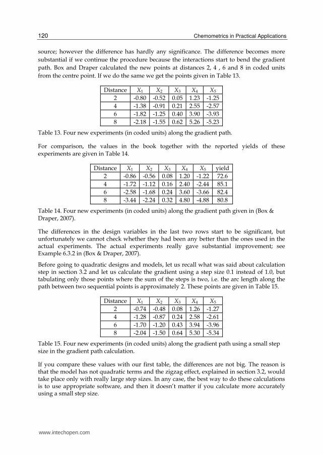
path. Box and Draper calculated the new points at distances 2, 4 , 6 and 8 in coded units
from the centre point. If we do the same we get the points given in Table 13.
Distance X1 X2 X3 X4 X5
2 -0.80 -0.52 0.05 1.23 -1.25
4 -1.38 -0.91 0.21 2.55 -2.57
6 -1.82 -1.25 0.40 3.90 -3.93
8 -2.18 -1.55 0.62 5.26 -5.23
Table 13. Four new experiments (in coded units) along the gradient path.
For comparison, the values in the book together with the reported yields of these experiments are given in Table 14.
Distance X1 X2 X3 X4 X5 yield
2 -0.86 -0.56 0.08 1.20 -1.22 72.6
4 -1.72 -1.12 0.16 2.40 -2.44 85.1
6 -2.58 -1.68 0.24 3.60 -3.66 82.4
8 -3.44 -2.24 0.32 4.80 -4.88 80.8
Table 14. Four new experiments (in coded units) along the gradient path given in (Box & Draper, 2007).
The differences in the design variables in the last two rows start to be significant, but unfortunately we cannot check whether they had been any better than the ones used in the actual experiments. The actual experiments really gave substantial improvement; see Example 6.3.2 in (Box & Draper, 2007).
Before going to quadratic designs and models, let us recall what was said about calculation step in section 3.2 and let us calculate the gradient using a step size 0.1 instead of 1.0, but tabulating only those points where the sum of the steps is two, i.e. the arc length along the path between two sequential points is approximately 2. These points are given in Table 15.
Distance X1 X2 X3 X4 X5
2 -0.74 -0.48 0.08 1.26 -1.27
4 -1.28 -0.87 0.24 2.58 -2.61
6 -1.70 -1.20 0.43 3.94 -3.96
8 -2.04 -1.50 0.64 5.30 -5.34
Table 15. Four new experiments (in coded units) along the gradient path using a small step size in the gradient path calculation.
If you compare these values with our first table, the differences are not big. The reason is that the model has not quadratic terms and the zigzag effect, explained in section 3.2, would take place only with really large step sizes. In any case, the best way to do these calculations is to use appropriate software, and then it doesn’t matter if you calculate more accurately using a small step size.
www.intechopen.com
Experimental Optimization and Response Surfaces
121
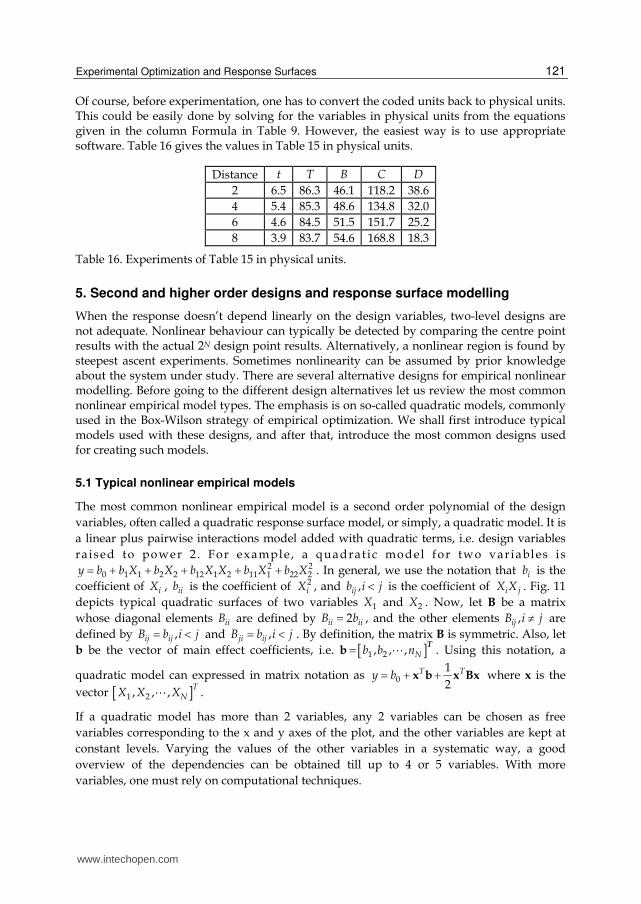
Of course, before experimentation, one has to convert the coded units back to physical units. This could be easily done by solving for the variables in physical units from the equations given in the column Formula in Table 9. However, the easiest way is to use appropriate software. Table 16 gives the values in Table 15 in physical units.
Distance t T B C D
2 6.5 86.3 46.1 118.2 38.6
4 5.4 85.3 48.6 134.8 32.0
6 4.6 84.5 51.5 151.7 25.2
8 3.9 83.7 54.6 168.8 18.3
Table 16. Experiments of Table 15 in physical units.
5. Second and higher order designs and response surface modelling
When the response doesn’t depend linearly on the design variables, two-level designs are not adequate. Nonlinear behaviour can typically be detected by comparing the centre point results with the actual 2N design point results. Alternatively, a nonlinear region is found by steepest ascent experiments. Sometimes nonlinearity can be assumed by prior knowledge about the system under study. There are several alternative designs for empirical nonlinear modelling. Before going to the different design alternatives let us review the most common nonlinear empirical model types. The emphasis is on so-called quadratic models, commonly used in the Box-Wilson strategy of empirical optimization. We shall first introduce typical models used with these designs, and after that, introduce the most common designs used for creating such models.
5.1 Typical nonlinear empirical models
The most common nonlinear empirical model is a second order polynomial of the design
variables, often called a quadratic response surface model, or simply, a quadratic model. It is
a linear plus pairwise interactions model added with quadratic terms, i.e. design variables
ra ised to power 2 . For example, a quadrat ic model for two var iables i s 2 2
0 1 1 2 2 12 1 2 11 1 22 2 y b b X b X b X X b X b X . In general, we use the notation that ib is the
coefficient of iX , iib is the coefficient of 2iX , and , ijb i j is the coefficient of i jX X . Fig. 11
depicts typical quadratic surfaces of two variables 1X and 2X . Now, let B be a matrix
whose diagonal elements iiB are defined by 2ii iiB b , and the other elements , ijB i j are
defined by , ij ijB b i j and , ji ijB b i j . By definition, the matrix B is symmetric. Also, let
b be the vector of main effect coefficients, i.e. 1 2, , ,b Nb b nT
. Using this notation, a
quadratic model can expressed in matrix notation as 0
1
2 x b x Bx
T Ty b where x is the
vector 1 2, , , TNX X X .
If a quadratic model has more than 2 variables, any 2 variables can be chosen as free
variables corresponding to the x and y axes of the plot, and the other variables are kept at
constant levels. Varying the values of the other variables in a systematic way, a good
overview of the dependencies can be obtained till up to 4 or 5 variables. With more
variables, one must rely on computational techniques.
www.intechopen.com

Chemometrics in Practical Applications
122
Fig. 11. Typical quadratic surfaces of 2 variables ( 1X and 2X ): a surface having a minimum
(upper left), a surface having a maximum (upper right), a surface having a saddle point
(lower left), and a surface having a ridge (lower right).
Other model alternatives are higher order polynomials, rational functions of several variables, nonlinear PLS, neural networks, nonlinear SVM etc. With higher order polynomials, or with linearized rational functions, it advisable to use ridge regression, PLS, or some other constrained regression technique, see e.g. (Taavitsainen, 2010). These alternatives are useful typically in cases where the response is bounded in the experimental region; see e.g. (Taavitsainen et. al., 2010).
5.2 Estimation and validation of nonlinear empirical models
Basically the analyses and techniques presented in sections 3.1.2 and 3.2 are applicable to
nonlinear models as well. Actually, polynomial models are linear in parameters, and thus
the theory of linear regression applies. Normally, nonlinear regression refers to regression
analysis of models that are nonlinear in parameters. This topic is not treated in this chapter,
and the interested reader may see e.g. (Bard, 1973)
It should be noted that some of the designs presented in section 5.3 are not orthogonal, and
therefore PLS or ridge regression are more appropriate methods than OLS for parameter
estimation, especially in so-called mixture designs.
www.intechopen.com

Experimental Optimization and Response Surfaces
123
For quadratic models, a special form of analysis called canonical analysis is commonly used for gaining better understanding of the model. However, this topic is beyond the scope of this chapter, and the reader is advised to see e.g. (Box & Draper, 2007). Part of the canonical analysis is to calculate the so called stationary point of the model. A stationary point is a point where the gradient with respect to the design variables vanishes. Solving for the stationary point is straightforward. The stationary point is the solution of the linear system of equations Bx b , obtained by differentiation from the model in matrix form given in
section 5.1. A stationary point can represent a minimum point, a maximum point, or a saddle point depending on the model coefficients.
5.3 Common higher order designs
Next we shall introduce the most common designs used for response surface modelling (RSM).
5.3.1 Factorial MN designs
Full factorial designs with M levels can be used for estimating polynomials of order at most 1M . Naturally, these designs are feasible only with very few variables, say maximum 3,
and typically for only few levels, say at most 4. For example, a 44 design would contain 256 which would be seldom feasible. However, the recent development in parallel microreactor systems having e.g. 64 simultaneously operating reactors at different conditions can make such designs reasonable.
5.3.2 Fractional factorial MN designs, and mixed level factorial design.
Sometimes it is known that one or more variables act nonlinearly and the others linearly. For
such cases a mixed level factorial design is a good choice. A simple way to construct e.g. a 3
or a 4 level mixed level factorial design is to combine a pair of variables in a 2N design into
a single new variable (Z) having 3 or 4 levels using the coding given in Table 17
( 1 2 3, ,x x x and 4x represent the levels of the variable constructed from a pair of variables
( ,i jX X ) in the original 2N design).
iX jX Z (3 levels) Z (4 levels)
-1 -1 1x 1x
-1 +1 2x 2x
+1 -1 2x 3x
+1 +1 3x 4x
Table 17. Construction of a 3, or 4 level variable from two variables of a 2N design.
There are also fractional factorial designs which are commonly used in Taguchi methodology. The most common such designs are the so-called Taguchi L9 and L27 orthogonal arrays, see e.g. (NIST SEMATECH).
www.intechopen.com

Chemometrics in Practical Applications
124
5.3.3 Box-Behnken designs
The structure and construction of Box-Behnken designs (Box & Behnken, 1960) is simple.
First, a 12 N design is constructed, say X0, then a 12 NN by N matrix of zeros X is created.
After this, X is divided into N blocks of 12 N rows and all columns, and in each block the
columns, omitting the i’th column, is replaced by X0. Finally one or more rows of N zeros are
appended to X. This is easy to program e.g. in Matlab or R starting from a 12 N design. The
following R commands will do the work for any number of variables (mton is a function
that generates NM designs, and nrep is the number of replicates at the centre point):
X0 <- as.matrix(mton(2,N-1)) M <- 2^(N-1) X <- matrix(0,N*M,N) for(i in 1:N) X[((i-1)*M+1):(M*i),(1:N)[-i]] <- X0 X <- rbind(X,rep(nrep,N))
As an example, Table 18 shows a Box-Behnken design of 3 variables and 3 centre point
replicate experiments.
1X 2X 3X
0 -1 -1
0 -1 +1
0 +1 -1
0 +1 +1
-1 0 -1
-1 0 +1
+1 0 -1
+1 0 +1
-1 -1 0
-1 +1 0
+1 -1 0
+1 +1 0
0 0 0
0 0 0
0 0 0
Table 18. A Box-Behnken design with 3 variables.
5.3.4 Central composite designs
The so-called central composite (CC) designs are perhaps the most common ones used in RSM, perhaps due their simple structure (for other possible reasons, see section 5.3). As the
name suggests they are composed of other designs, namely, of a factorial or fractional 2N
www.intechopen.com

Experimental Optimization and Response Surfaces
125
part, of so-called axial points, and of centre points. Sometimes the latter two parts together are called a star design. As an example, Table 19 shows a CC design for two variables.
1X 2X
-1 -1
Facto
rial 22
part
-1 +1 +1 -1
+1 +1 0 Axial
po
ints
0 0
0 0 0 Centre
points 0 0
Table 19. A CC design with 2 variables.
The value depends on the kind of properties we want the design to have. Typical desired
properties are orthogonality, rotatability, and symmetry. A rotatable design is such that the
prediction variance of a point in the design space does depend only on its distance from.
design centre, not on its direction. Let us denote the number of the centre points by cpN .
Then, for an orthogonal design is given by the following Eq. 11.
12 42
2 2 24
N
N NcpN N (11)
The derivation of this rather formidable looking equation, and of the two following ones, are
given e.g. in (Box & Draper, 2007). It should be noted that the model matrix obtained with
this choice for is not strictly orthogonal, because the intercept column (the column of
ones) vector is not orthogonal to the column vector of the quadratic terms. However, all the
other columns of the model matrix are orthogonal to each other. This can also be expressed
by saying that the quadratic effects are partially confounded with the intercept.
For a rotatable design, the appropriate value for is given by the equation Eq. 12.
42 N (12)
For maximal symmetry, i.e. all points except for the centre point, lie on a hypersphere of radius , the appropriate value for is given by the equation Eq. 13
N (13)
A common fourth choice is to set to 1. Such CC design is called a face centred CC design
(CCF). For ’s greater than 1 the designs are called circumscribed, CCC. Some other
alternatives, e.g. compromising between orthogonality and rotatability, exist too. Sometimes a CCC design is scaled so that is scale to 1, and the coordinates of the factorial points are
www.intechopen.com
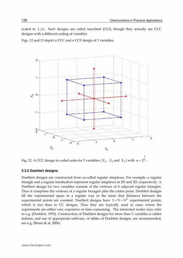
Chemometrics in Practical Applications
126
scaled to 1 / . Such designs are called inscribed (CCI), though they actually are CCC
designs with a different coding of variables.
Figs. 12 and 13 depict a CCC and a CCF design of 3 variables.
Fig. 12. A CCC design in coded units for 3 variables ( 1X , 2X and 3X ) with 3
42 .
5.3.5 Doehlert designs
Doehlert designs are constructed from so-called regular simplexes. For example, a regular
triangle and a regular tetrahedron represent regular simplexes in 2D and 3D, respectively. A
Doehlert design for two variables consists of the vertexes of 6 adjacent regular triangles.
Thus it comprises the vertexes of a regular hexagon plus the centre point. Doehlert designs
fill the experimental space in a regular way in the sense that distances between the
experimental points are constant. Doehlert designs have 21 N N experimental points,
which is less than in CC designs. Thus they are typically used in cases where the
experiments are either very expensive or time consuming. The interested reader may refer
to e.g. (Doehlert, 1970). Construction of Doehlert designs for more than 2 variables is rather
tedious, and use of appropriate software, or tables of Doehlert designs, are recommended,
see e.g. (Bruns & al, 2006)
www.intechopen.com

Experimental Optimization and Response Surfaces
127
Fig. 13. A CCF design in coded units for 3 variables ( 1X , 2X and 3X ) with 1 .
5.3.6 Mixture designs
If the design variables are proportions of constituents in a mixture, then in each experiment the values of the design variables sum up to 1 (100 %). In such cases, ordinary designs cannot be applied, since the row sums of ordinary designs vary irrespective of the coding used. If there are no other constraints than the closure constraint, the most common designs are the so-called simplex lattice, and simplex centroid designs. If some constraints are imposed as well, a good choice is to use optimal designs (see the next section), though other alternatives exist as well; see e.g. (Cornell, 1981), or (Montgomery, 1991).
The closure constraint has to be taken into account also in modelling results of mixture experiments. The closure means that the columns of the model matrix are linearly dependent making the matrix singular. One way to overcome this problem is to make the model using only 1N variables, because we need to know only the values of 1N
variables, and the value of the N’th variable is one minus the sum of the others. However, this may make the interpretation of the model coefficients quite difficult. Another alternative is to use the so-called Scheffe polynomials, i.e. polynomials without the intercept and the quadratic terms. It can be shown that Scheffe polynomials of N variables represent the same model as an ordinary polynomial of 1N variables, naturally with different
values for the polynomial coefficients. For example the quadratic polynomial of two
www.intechopen.com
Chemometrics in Practical Applications
128
variables 1 1 2 2 12 1 2 y b X b X b X X can be simplified into 22 1 2 12 1 12 1 y b b b b X b X if
2 11 X X . This shows that it is a quadratic function of 1X only; for more details see e.g.
(Cornell, 1981).
The model matrices of mixture designs are not orthogonal, and they are usually quite ill-conditioned. For this reason, it is commonly recommended to use PLS or ridge regression for estimating the model parameters.
5.3.7 Optimal designs
The idea behind so-called optimal designs is to select the experimental points so that they satisfy some optimality criterion about the model to be used. It is important to notice that the optimality of such designs is always dependent on the model. For this reason, optimal designs are often used in designing experiments for mechanistic modelling problems. In empirical modelling we don’t know the model representing the ‘true’ behaviour, and even a good empirical model is just an approximation of the true behaviour. Of course, if it has been decided to use e.g. a quadratic approximation, using a design that is optimal for a quadratic model is perfectly logical. However, the design still should have extra experiments that allow assessing the lack-of-fit.
Typically optimal designs are planned for quadratic models. Probably the most common optimality criterion is the D-optimality criterion. A D-optimal design is a design that
minimizes the determinant of the information matrix, i.e. 1
X XT where X is the model
matrix. There are several other optimality criteria, typically related to minimizing the variance of predictions, or to minimizing the variances of the model parameter estimates. In many cases, a design that is optimal according to one criterion is also optimal or nearly optimal according to several other criteria as well.
A nice feature in optimal designs is that it is easy take into account constraints in the design
space, e.g. a mixture constraint, or a constraint in which one variable always has to have a
greater value than some other variable. Constraints can sometimes be handled by some
‘tricks’, e.g. instead of using 1x and 2x when 1 2x x , one could use in design 1x and 3x
and set 2 1 3 x x x , i.e. to use a variable that tells how much greater to the value of 1x the
value of 2x is. In general, using optimal designs is the most straightforward approach for
constrained problems.
In practice, constructing optimal designs requires suitable software. Optimal design routines are available in most commercial statistical software packages containing tools for DOE. There is also an R package for creating optimal designs, called AlgDesign (http://cran.r-project.org/web/packages/AlgDesign/index.html). See also (Fedorov, 1972) or (Atkinson et. al., 2007).
5.4 Choosing an appropriate second order design
As we have seen, there are many types of designs for nonlinear empirical (usually quadratic) models. How does a practitioner know which one to choose? A good strategy is to try first a simple design that has extra degrees of freedom for validation and for checking
www.intechopen.com

Experimental Optimization and Response Surfaces
129
model adequacy. Of course, if the problem at hand is a mixture problem, one has to rely on mixture designs or optimal designs. If the experiments are very expensive, one may have to use saturated, or almost saturated designs, e.g. optimal designs or Doehlert designs. In other cases CC or Box-Behnken designs are better choices. For 3 variables, a Box-Behnken design contains fewer experiments than a CC design for 3 variables, but for more variables it is the other way round. For example, a 4 variable Box-Behnken design (without replicates) contains 33 experiments, as the corresponding CC design contains 25 experiments. Thus, except for mixture problems or constrained problems, a CC design is usually the best choice. In general, CCC designs should be preferred to CCF designs, but otherwise choosing the value for is usually not a big issue from the practical point of view; the differences in
performance are minor. CCF designs should be used only in cases where there is a real benefit of having fewer variable levels than the 5 variable levels of CCC designs (CCF designs use only 3 variable levels).
5.5 Example: Analysis of a Doehlert design for two variables
This example comes from (Dos Santos et. al., 2008). The aim was to optimize the recovery
percentage of several elements with respect to the temperature and the volume of
concentrated nitric acid from which we take only the recovery percentage of manganese (for
details, see (Dos Santos et. al., 2008). The design is a Doehlert design with 3 replicates, and it
is given in physical units in Table 20.
Temperature Volume Recovery %
135 5 89.0
165 5 90.2
120 3 90.4
150 3 94.3
150 3 91.6
150 3 91.2
180 3 91.0
135 1 82.6
165 1 88.0
Table 20. A Doehlert design with 2 variables.
Next, the variables are coded so that the maximum values are set to +1 and the minimum
values are set to 1 . Thus the coding formulas will be 1150
30
TX , and 2
3
2
VX . The
design in coded units is given in Table 21.
www.intechopen.com

Chemometrics in Practical Applications
130
1X 2X Recovery %
-0.5 +1 89.0
0.5 +1 90.2
-1 0 90.4
0 0 94.3
0 0 91.6
0 0 91.2
+1 0 91.0
-0.5 -1 82.6
+0.5 -1 88.0
Table 21. A Doehlert design with 2 variables in coded units.
Fig. 14 shows the design together with the recoveries visualizing the hexagonal structure of the design.
Fig. 14. The design of example 5.4.1 together with the measured recovery percentages.
www.intechopen.com

Experimental Optimization and Response Surfaces
131
Next a quadratic model is fitted to the data. The parameter estimates and the related statistics are given in Table 22.
Estimate Std. Error t value p value
(Intercept) 92.37 1.14 81.06 4.14e-06
X1 1.30 1.14 1.14 0.337
X2 2.15 0.99 2.18 0.118
I(X1^2) -1.67 1.80 -0.93 0.423
I(X1 * X2) -2.10 1.97 -1.06 0.365
I(X2^2) -4.50 1.35 -3.33 0.045
Residual standard error: 1.974 on 3 degrees of freedom Multiple R-squared: 0.8594, Adjusted R-squared: 0.6251 F-statistic: 3.668 on 5 and 3 DF, p-value: 0.1569
Table 22. Regression summary of the quadratic model.
According to Table 22 only the intercept and the quadratic effect of 2x are significant. The
p-value of the lack-of-fit test based on the 3 replicates is ca. 0.28. Thus the lack-of-fit is not
significant. The apparent reason for the low significance is the rather poor repeatability of
the experiments. The standard deviation of the recoveries of the replicate experiments is ca.
1.68 which is relatively high compared to the overall variation in the recoveries.
Next, let us see the results of cross-validation. Before cross-validation, the 3 replicates are replaced by the average of them. Fig. 15 shows the cross-validation results.
According to the cross-validation the predictions of the model are not very good. Due to the
poor repeatability, i.e. large experimental error, it is hard to tell whether the reason for
unreliable prediction is the large experimental error or something else, e.g. more
complicated nonlinearity than quadratic one. According to the model, the optimum lies
inside the experimental region and it corresponds to the stationary point. The optimal point
in coded units is 1 0.25X and 2 0.17X which corresponds to T = 158 and V = 3.35 in
physical units. This should be compared to Fig. 16 which shows the corresponding response
surface.
6. Multi-response optimization
A common problem is to optimize the values of several responses simultaneously. This
occurs quite frequently, because many products have to meet several different goodness
criteria. The problem in such applications is that the individual optima can be contradictory,
i.e. the optimal values for one of the responses may be far from the optimal values for some
other response. Several different techniques, such as finding the so-called Pareto optimal
result, exist. By far the simplest approach to this problem is to use so-called desirability
functions, presented in the next section. The idea was first presented by (Derringer & Suich,
1980) in an application of product development in rubber industry.
Optimization using the desirability function technique can be divided into the following steps:
www.intechopen.com

Chemometrics in Practical Applications
132
Fig. 15. Cross-validation of the quadratic model. Left panel: Recovery % vs. the number of experiment; black circles: data; blue triangles: fitted values; red pluses: cross-validated leave-one-out prediction. Right panel: Normal probability plots of the cross-validated leave-one-out residuals.
www.intechopen.com

Experimental Optimization and Response Surfaces
133
Fig. 16. Recovery % vs. Temperature and Volume.
First make a regression model, based on the designed experiments, individually for each response. Validate the models and proceed to step 2 after all models are satisfactory.
Make a desirability function i i id D y for each response separately (i goes from 1 to the
number responses, say q). Remember that the responses have been modelled as functions of
the design variables, i.e. 1 2, , , i i Ny f X X X .
Building the desirabilities should be done together with a person who knows what the customers want from the product, and it is typically team work. How to build such functions in practice is explained later. Note that combining the two functions, desirabilities can be expressed as functions of design variables only.
www.intechopen.com

Chemometrics in Practical Applications
134
Use an optimizer to maximize the combined desirability D which is the geometric mean of
the individual desirabilities, i.e. 1
1 2 qqD D D D , with respect to the design variables.
Check by experimentation that the found optimum really gives a good product.
There are many ways to produce suitable desirability functions, one of which is explained in (Derringer & Suich, 1980). Any function that gives the 1 value for a perfect response and the value 0 for an unacceptable product and continuously values between 0 and 1 for responses whose goodness is in-between unacceptable and perfect can be used. One of the simplest
alternatives is to use the following functions:
1
1
iy a
bid e for one-sided desirabilities,
and
c
iy a
bid e for two-sided desirabilities. The parameters a, b and c are user-defined
parameters chosen with the help of an expert on the product quality.
The idea is best illustrated by an example. Let us consider an example where the product would be the better the higher its elasticity is. Let us also assume that elasticity from 0.60 upwards would mean a practically perfect product and elasticity below 0.30 would mean a totally unacceptable product. Then the one-sided desirability function looks like (with a = 0.46 and b = 0.028) the one given in Fig. 17.
Fig. 17. A one-sided desirability function for elasticity that should be 0.60 or more and that would be totally unacceptable below 0.30.
www.intechopen.com
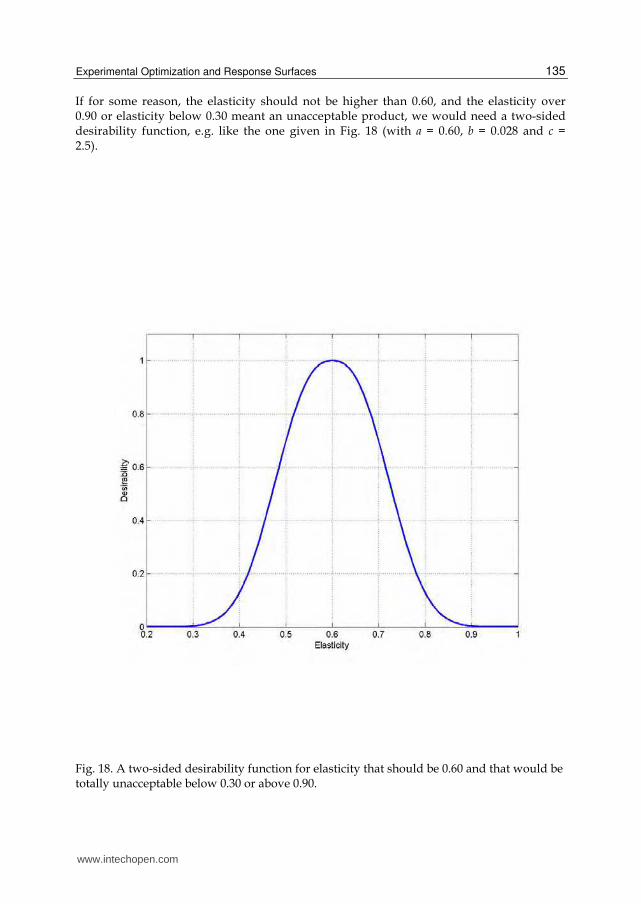
Experimental Optimization and Response Surfaces
135
If for some reason, the elasticity should not be higher than 0.60, and the elasticity over 0.90 or elasticity below 0.30 meant an unacceptable product, we would need a two-sided desirability function, e.g. like the one given in Fig. 18 (with a = 0.60, b = 0.028 and c = 2.5).
Fig. 18. A two-sided desirability function for elasticity that should be 0.60 and that would be totally unacceptable below 0.30 or above 0.90.
www.intechopen.com

Chemometrics in Practical Applications
136
For practical examples see e.g. (Taavitsainen et. al., 2010) or (Laine et. al., 2011).
7. Conclusion
Design of experiments is as much of an art as of science. Becoming an expert in the field
requires both theoretical studies and experience in practical applications. Although many
problems can be solved in principle by hand calculations, in practice use of suitable software
is needed. If the person involved is not familiar with command line style programs whose
use is essentially that of programming, he or she is recommended to use some commercial
software that typically also guide the user in the design and in the analysis of the results.
The use of simulation models, where artificial experimental error is added into the results of
the simulation, is highly recommended.
8. Acknowledgment
This work has been supported by the Helsinki Metropolia University of Applied Sciences.
9. References
Atkinson, A., Donev, A. & Tobias, R. (2007). Optimum experimental designs, with SAS. Oxford
University Press, ISBN 978-0-19-929660-6, New York, USA
Bard, Y. (1973) Nonlinear Parameter Estimation, Academic Press, ISBN 978-0120782505, New
York, USA
Bayne, K. & Rubin, I. (1986). Practical Experimental Designs and Optimization Methods for
Chemists, VCH, ISBN 0-89573-136-3, Deerfield Beach, Florida, USA
Berthouex, P. & Brown, L. (2002). Statistics for Environmental Engineers, Lewis Publishers
(CRC), ISBN 1-56670-592-4, Boca Raton, Florida, USA
Box, G. & Behnken, D. (1960). A simplex method for function minimization. Technometrics,
Vol.2, No.4, pp. 455–475
Box, G. & Draper. (2007). Response Surfaces, Mixtures, and Ridge Analyses, Wiley (2nd ed.),
ISBN 978-0-470-05357-7, Hoboken, New Jersey, USA
Box, G., Hunter, Hunter. (2005). Statistics for Experimenters: Design, Innovation, and Discovery
(2nd ed.),Wiley, ISBN 978-0-471-71813-0, New York, USA
Bruns, R., Scarmiano, I. & de Barros Neto, B. (2006). Statistical Design - Chemometrics ,
Elsevier, ISBN 978-0-444-52181-1, Amsterdam, The Netherlands
Carlson, R. & Carlson, R. (2005). Design and optimization in organic synthesis, Elsevier
Cornell, J. (1981). Experiments with Mixtures: Designs, Models, and the Analysis of Mixture Data
(3rd ed.), Wiley, ISBN 0-471-07916-2, New York, USA
Derringer, G. & Suich, R. (1980), Simultaneous Optimization of Several Response Variables.
Journal of Quality Technology, Vol.12, pp. 214-219
Doehlert, D. (1970) Uniform shell designs. Applied Statistics, Vol.19, pp.231-239.
Dos Santos, W., Gramacho, D., Teixeira, A., Costa,A. & Korn, M. (2008), Use of Doehlert
Design for Optimizing the Digestion of Beans for Multi-Element Determination by
www.intechopen.com

Experimental Optimization and Response Surfaces
137
Inductively Coupled Plasma Optical Emission Spectrometry, J. Braz. Chem. Soc.,
Vol. 19, No. 1, pp.1-10.
Efron, B., Hastie, T., Johnstone. I. & Tibshirani, R. (2004), Least angle regression, Ann. Statist.
Vol. 32, No. 2, pp. 407-499.
Fedorov, V. (1972). Theory of Optimal Experiments. Academic Press, ISBN 978-0824778811,
New York, USA
Haaland, P. (1989). Experimental Design in Biotechnology, Marcel Dekker, ISBN 978-
0824778811, New York, USA
Hanrahan, G. (2009). Environmental Chemometrics, CRC Press, ISBN 978-1420067965, Florida,
USA
Himmelblau, D. (1970). Process Analysis by Statistical Methods, Wiley, ISBN 978-0471399858 ,
New York, USA
JMP, release 6, Design of Experiments,
http://www.jmp.com/support/downloads/pdf/jmp_design_of_experiments.pdf,
9.9.2011
Kolarik, W. (1995). Creating Quality, McGraw-Hill, ISBN 0-07-113935-4
Koljonen, J., Nordling, T. & Alander, J. (2008), A review of genetic algorithms in near
infrared spectroscopy and chemometrics: past and future, Journal Of Near Infrared
Spectroscopy, Vol. 16, No. 3, pp. 189-197
Laine, P., Toppinen, E., Kivelä, R., Taavitsainen, V-M., Knuutila, O., Sontag-Strohm,
T.,Jouppila, K. & Loponen, J.(2011), Emulsion preparation with modified oat bran:
Optimization of the emulsification process for microencapsulation purposes,
Journal of Food Engineering, Vol.104, pp.538-547
Montgomery, D. (1991). Design and Analysis of Experiments (3rd ed.), Wiley, ISBN 0-471-
52994-X, Singapore
Nelder, J. & Mead, R. (1965). A simplex method for function minimization. Computer Journal
Vol.7, No.4, pp. 308–313, ISSN 0010-4620
Neter, J., Kutner, M., Nachtsheim, C. & Wasserman, W. (1996), Applied Linear Statistical
Models (4th ed.), WCB/McGraw-Hill, ISBN 0-256-11736-5, Boston, Massachusetts,
USA
NIST/SEMATECH e-Handbook of Statistical Methods,
http://www.itl.nist.gov/div898/handbook/, 9.8.2011
Taavitsainen, V-M. Ridge and PLS based rational function regression (2010), Journal of
Chemometrics. Vol.24, No. 11-12, pp.665-673
Taavitsainen, V-M., Lehtovaara, A. & Lähteenmäki, M. (2010), Response surfaces,
desirabilities and rational functions in optimizing sugar production, Journal of
Chemometrics. Vol. 24, No. 7-8, pp. 505-513
Tibshirani, R. (1996), Regression shrinkage and selection via the lasso, J. Royal. Statist. Soc. B.
Vol. 58, pp. 267–288
Vardeman, S. (1994). Statistics for Engineering Problem Solving, PWS , ISBN 978-0780311183,
Boston, Massachusetts, USA
Weisberg, S. (1985). Applied Linear Regression, Wiley, ISBN 0-471-87957-6, New York,
USA
www.intechopen.com

Chemometrics in Practical Applications
138
Wheeler, R. (1974) Portable power , Technometrics, Vol. 16, No. 2, pp. 193-201
Zou, H. & Hastie, T. (2005), Regularization and Variable Selection via the Elastic Net, Journal
of the Royal Statistical Society, Series B, Vol. 76, pp. 301-320.
www.intechopen.com

Chemometrics in Practical ApplicationsEdited by Dr. Kurt Varmuza
ISBN 978-953-51-0438-4Hard cover, 326 pagesPublisher InTechPublished online 23, March, 2012Published in print edition March, 2012
InTech EuropeUniversity Campus STeP Ri Slavka Krautzeka 83/A 51000 Rijeka, Croatia Phone: +385 (51) 770 447 Fax: +385 (51) 686 166www.intechopen.com
InTech ChinaUnit 405, Office Block, Hotel Equatorial Shanghai No.65, Yan An Road (West), Shanghai, 200040, China
Phone: +86-21-62489820 Fax: +86-21-62489821
In the book "Chemometrics in practical applications", various practical applications of chemometric methods inchemistry, biochemistry and chemical technology are presented, and selected chemometric methods aredescribed in tutorial style. The book contains 14 independent chapters and is devoted to filling the gapbetween textbooks on multivariate data analysis and research journals on chemometrics andchemoinformatics.
How to referenceIn order to correctly reference this scholarly work, feel free to copy and paste the following:
Veli-Matti Tapani Taavitsainen (2012). Experimental Optimization and Response Surfaces, Chemometrics inPractical Applications, Dr. Kurt Varmuza (Ed.), ISBN: 978-953-51-0438-4, InTech, Available from:http://www.intechopen.com/books/chemometrics-in-practical-applications/experimental-optimization-and-response-surfaces