experimental investigation of the effects of fuel aging on ... · performance and emissions of...
TRANSCRIPT
Experimental Investigation of the Effects of Fuel Aging on
Combustion Performance and Emissions of Biomass Fast
Pyrolysis Liquid-Ethanol Blends in a Swirl Burner
by
Milad Zarghami-Tehran
A thesis submitted in conformity with the requirements
for the degree of Master of Applied Science
Graduate Department of Mechanical and Industrial Engineering
University of Toronto
Copyright© by Milad Zarghami-Tehran 2012

ii
Abstract
Experimental Investigation of the Effects of Fuel Aging on Combustion
Performance and Emissions of Biomass Fast Pyrolysis Liquid-Ethanol
Blends in a Swirl Burner
Milad Zarghami-Tehran
Master of Applied Science
Graduate Department of Mechanical and Industrial Engineering
University of Toronto
2012
Biomass fast pyrolysis liquid is a renewable fuel for stationary heat and power generation;
however degradation of bio-oil by time, a.k.a. aging, has an impact on combustion performance
and emissions. Moreover, the temperature at which bio-oil is stored has a strong effect on the
degradation process. In this study, the same biooil-ethanol blends with different storage
conditions are tested in a pilot stabilized spray burner under the same flow conditions.
Measurements were made of the steady state gas phase emissions and particulate matter, as well
as visual inspection of flame stability. The results confirm a relationship between room
temperature storage time and storage at higher temperatures (accelerated aging). They also show
that fuel aging increases the emissions of carbon monoxide, unburned hydrocarbon and the
organic fraction of particulate matter. These emissions increase more rapidly as more time is
allocated for aging. NOx emission shows a slight decrease with fuel aging.

iii
Acknowledgements
I would like to thank Professor Murray J. Thomson for his guidance and supervision during the
course of this project. My mother and sister also deserve a special appreciation for their support
during this project.
Dr. Tommy Tzanetakis was my mentor, and I appreciate his endless support during various
stages of this project. I am thankful to Sina Moloodi, because of his generous advice whenever a
problem came up and his patience in teaching me how to operate the setup. I am also grateful for
all the support and help received from Brian Nguyen during the reconstruction of the lab and
running the experiments.
Many thanks to Umer Khan and Babak Borshanpour for their help during the experiments. I
would also like to thank R. Rizvi and Professor H. Naquib for their help with the
thermogravimetric analyzer. The help and support of other combustion research group members,
especially, Meghdad, Armin and Reza is gratefully appreciated.
Finally, I would like to acknowledge Natural Sciences and Engineering Research Council
(NSERC) of Canada, as well as Advanced Biorefinery Innovation Network (ABIN) for their
financial support and funding.
iv
Table of Contents
Abstract ........................................................................................................................................... ii
Acknowledgements ........................................................................................................................ iii
Table of Contents…………………………………………………………………………………iv
List of Tables ............................................................................................................................... viii
List of Figures ................................................................................................................................ ix
Nomenclature ................................................................................................................................ xii
1. Introduction ............................................................................................................................. 1
1.1 Motivation ........................................................................................................................ 1
1.2 Objective .......................................................................................................................... 2
2. Literature Review .................................................................................................................... 3
2.1 Bio-oil Production ............................................................................................................ 3
2.2 Bio-oil Properties ............................................................................................................. 4
2.2.1 Acidity ....................................................................................................................... 4
2.2.2 Oxygen & Water Content vs. Heating Value ............................................................ 5
2.2.3 Viscosity ................................................................................................................... 5
2.2.4 Solids Content ........................................................................................................... 5
2.2.5 Ash Content .............................................................................................................. 6
2.2.6 Evaporative Residue ................................................................................................. 7
2.2.7 Storage Stability ........................................................................................................ 8
2.3 Aging Mechanisms ........................................................................................................... 9
2.3.1 Esterification ............................................................................................................. 9
2.3.2 Polymerization .......................................................................................................... 9
2.3.3 Air Oxidation .......................................................................................................... 10
2.3.4 Gas Forming ............................................................................................................ 10

v
2.4 Effects of aging on bio-oil properties ............................................................................. 12
2.4.1 Visual & Structural Changes .................................................................................. 12
2.4.2 Viscosity ................................................................................................................. 13
2.4.3 Water Content ......................................................................................................... 15
2.4.4 Average Molecular Weight ..................................................................................... 17
2.4.5 Volatility ................................................................................................................. 19
2.4.6 Phase Separation ..................................................................................................... 20
2.5 Methods to Slow Down Aging ....................................................................................... 20
2.5.1 Solvent Addition ..................................................................................................... 20
2.5.2 Very mild hydrogenation ........................................................................................ 22
2.5.3 Minimizing the exposure to air ............................................................................... 23
2.6 Droplet Combustion of Bio-oil ...................................................................................... 23
2.7 Effect of Bio-oil Properties on Spray Combustion ........................................................ 25
2.7.1 Viscosity ................................................................................................................. 25
2.7.2 TGA Residue .......................................................................................................... 26
2.7.3 Water Content ......................................................................................................... 27
2.7.4 Solids & Ash Content ............................................................................................. 28
3. Experimental Methodology .................................................................................................. 30
3.1 Spray Burner .................................................................................................................. 30
3.1.1 Overall Setup .......................................................................................................... 31
3.1.2 Variable Swirl Generator ........................................................................................ 32
3.1.3 Air-Blast Atomizing Nozzle ................................................................................... 34
3.1.4 Pilot Flame .............................................................................................................. 35
3.2 Fuel Analysis .................................................................................................................. 36
3.2.1 Fuel Composition & Heating Value ....................................................................... 36
3.2.2 Viscosity ................................................................................................................. 37

vi
3.2.3 Thermogravimetric Analysis .................................................................................. 37
3.3 Gas Phase Emissions Measurement ............................................................................... 38
3.3.1 Oxygen Concentration ............................................................................................ 38
3.3.2 Unburned Hydrocarbons ......................................................................................... 39
3.3.3 Detailed Speciation of Pollutants ............................................................................ 39
3.4 Particulate Matter Emissions Measurement ................................................................... 41
3.4.1 Isokinetic Sampling System .................................................................................... 41
3.4.2 Gravimetric & Loss on Ignition Analysis ............................................................... 46
3.5 Flame Visualization ........................................................................................................ 48
3.6 Aging Procedure ............................................................................................................. 49
3.7 Combustion Test Procedure ........................................................................................... 51
4. Results and Discussion ......................................................................................................... 55
4.1 Experimental Test Plan .................................................................................................. 55
4.2 Experimental Results Summary ..................................................................................... 56
4.3 Mechanism of Pollution Formation from Bio-oil Combustion ...................................... 58
4.4 Analysis on the First Batch: Natural vs. Accelerated Aging .......................................... 60
4.4.1 Fuel Properties ........................................................................................................ 60
4.4.2 Gaseous Emissions .................................................................................................. 63
4.4.3 PM Emissions ......................................................................................................... 65
4.4.4 Flame Visualization ................................................................................................ 67
4.5 Analysis on the Second Batch: Long Term Accelerated Aging ..................................... 68
4.5.1 Fuel Properties ........................................................................................................ 68
4.5.2 Gaseous Emissions .................................................................................................. 72
4.5.3 PM Emissions ......................................................................................................... 73
4.5.4 Flame Visualization ................................................................................................ 75
4.6 NOx Emissions ............................................................................................................... 76

vii
4.7 Acetaldehyde, Formaldehyde and Methane Emissions .................................................. 78
5. Conclusions and Recommendations ..................................................................................... 79
5.1 Conclusions .................................................................................................................... 79
5.2 Recommendations .......................................................................................................... 80
5.3 Future Works .................................................................................................................. 80
Bibliography ................................................................................................................................. 82
Appendix A- Theoretical Isokinetic Sampling System Calibration ............................................. 88
Appendix B- Liquid and Gaseous Flow Calibration ..................................................................... 90
Appendix C- FTIR Calibration Validation ................................................................................... 92
Appendix D- Example of the TGA Curve .................................................................................... 93
Appendix E- Data Acquisition System ......................................................................................... 94

viii
List of Tables
Table 2.1 – Effect of Aging Time and Temperature on Water Content [27] ................................ 16
Table 2.2 – Effect of Aging on Average Molecular Weight of Bio-oil [27] ................................ 18
Table 3.1 – Fuel properties measurement standards ..................................................................... 36
Table 3.2 – Detection limits and uncertainty levels of the FTIR calibration model ..................... 40
Table 3.3 – Calculation methods of each PM fraction .................................................................. 47
Table 4.1 – Base point Operating Condition ................................................................................ 56
Table 4.2 – Basic Fuel Properties and Emissions of Aged Pure Bio-oil ...................................... 57
Table 4.3 - NOx Emissions of the Aged Bio-oil ............................................................................ 58
Table 4.4 – Emissions for Selected Blends ................................................................................... 78

ix
List of Figures
Figure 2.1- Fast Pyrolysis Process [10] .......................................................................................... 4
Figure 2.2 – Viscosity vs. Temperature and Methanol Addition [19] ............................................ 6
Figure 2.3 – TGA curves for batches with different solid content [22] .......................................... 8
Figure 2.4 – Changes of Waxy material morphology during Aging [38] ..................................... 12
Figure 2.5 - Viscosity of bio-oils and bio-oils with solvent addition at 60°C [39] ...................... 13
Figure 2.6 – Viscosity of bio-oil from softwood bark aged at 80 C [40] ..................................... 14
Figure 2.7 – Effect of Storage Time and Measurement Temperature on Viscosity [25] .............. 14
Figure 2.8 – Rate of viscosity increase vs. time of storage [37] ................................................... 15
Figure 2.9 – Effect of Aging and Solvent Addition on Water Content [39] ................................. 15
Figure 2.10 – Effect of Water Content and Methanol on Aging Rate [32] .................................. 16
Figure 2.11 – Effect of Aging on Bio-oil Constituents [37] ......................................................... 17
Figure 2.12 – Effect of Aging on Different Molecular Weight Compounds [25] ........................ 19
Figure 2.13 – Effect of Aging on Volatility [25] .......................................................................... 19
Figure 2.14 – Effects of additives on aging [32] .......................................................................... 22
Figure 2.15 – Four Stages of Bio-oil Droplet Combustion (left to right) [43] ............................. 24
Figure 2.16 – Solid State Combustion of the Cenospheric Residue [43] ..................................... 24
Figure 2.17 – Effect of SMD on Combustion [46] ....................................................................... 26
Figure 2.18 – Effect of TGA Residue on Combustion [22] .......................................................... 27
Figure 2.19 – Effect of Water Content on Combustion [22] ........................................................ 28
Figure 2.20 – Effect of Solids Content on Combustion [22] ........................................................ 29
Figure 3.1 – Bio-oil Burner Assembly [46] .................................................................................. 30
Figure 3.2 – Overall schematic of experimental setup [46] .......................................................... 32
Figure 3.3 – Schematic of Movable Block Swirl Generator [46] ................................................. 33
Figure 3.4 - CRZ of swirling flows in confined geometry [50] .................................................... 33
Figure 3.5 – Atomizing Nozzle Tip Assembly [52] ..................................................................... 34
Figure 3.6 – Schematic of Nozzle Cooling System [22] .............................................................. 35
Figure 3.7 – Alignment of Pilot Flame [46] ................................................................................. 36
Figure 3.8 – Schematic of the gas phase emissions measurement system [46] ............................ 38
Figure 3.9 – Gas Streamlines around sampling probe (VS < V) ................................................... 42
Figure 3.10 – Schematic of PM sampling system [46] ................................................................. 44

x
Figure 3.11 – Geometry and position of sampling probe and pressure taps [46] ......................... 45
Figure 3.12 – Gravimetric analysis and Loss on ignition procedure [22] .................................... 47
Figure 3.13 – Borescope Assembly [46] ....................................................................................... 48
Figure 3.14 – Temperature vs Time for Natural Aging ................................................................ 50
Figure 4.1 – Pollutant Formation Mechanisms of Bio-oil Combustion [22] ................................ 59
Figure 4.2 – Calculated Viscosity of Batch 1 Pure Bio-oil (via handheld viscometer) over Aging
Time .............................................................................................................................................. 61
Figure 4.3 – Measured Viscosity of Batch 1 Pure Bio-Oil (based on ASTM D445) over aging
time ............................................................................................................................................... 62
Figure 4.4 – Solids Content of Batch 1 Pure Bio-oil vs. Aging Time .......................................... 62
Figure 4.5 – Effect of Aging on the first batch blends’ TGA residue .......................................... 63
Figure 4.6 – CO emissions for Batch 1 Blends vs. Aging Time ................................................... 64
Figure 4.7 - UHC emissions for Batch 1 Blends vs. Aging Time ................................................ 64
Figure 4.8 – CR Emissions of Batch 1 Blends over the Aging Period ......................................... 66
Figure 4.9 – Comparison of Calculated and Measured CR for Batch 1 Blends ........................... 67
Figure 4.10 – Borescopic Photos of batch 1 bio-oil blend combustion ........................................ 68
Figure 4.11 - Calculated Viscosity of Batch 2 (via handheld viscometer) over Aging Time ....... 69
Figure 4.12 - Measured Viscosity of Batch 2 (based on ASTM D445) over Aging Time .......... 70
Figure 4.13 - Solids Content of Batch 1 vs. Aging Time ............................................................ 71
Figure 4.14 - Effect of Aging on the second batch blends’ TGA residue .................................... 72
Figure 4.15 - CO emissions for Batch 2 vs. Aging Time ............................................................. 73
Figure 4.16 - CO emissions for Batch 2 vs. Aging Time ............................................................. 73
Figure 4.17 - CR Emissions of Batch 2 Blends over the Aging Period ........................................ 74
Figure 4.18 - Comparison of Calculated and Measured CR for Batch 2 Blends .......................... 75
Figure 4.19 – Borescopic Photos of batch 2 bio-oil blends combustion ...................................... 76
Figure 4.20 – NOx emissions of Batch 1 Blends over Aging Period ........................................... 77
Figure 4.21 - NOx emissions of batch 2 over Aging Period ........................................................ 78
Figure A.1 – Velocity profile for the exhaust flow ....................................................................... 88
Figure C.1 – 1500 ppm CO spectrums before and after changing the FTIR He-Ne laser ............ 92
Figure D.1 – TGA curve for bio-oil blend 1N3 ............................................................................ 93
Figure E.1 – Front View of the Labview Program ....................................................................... 95
Figure E.2 – Logged Temperatures for Bio-oil blend 1A24 ......................................................... 96

xi
Figure E.3 – oxygen sensor voltage for bio-oil blend 1A24 ......................................................... 96

xii
Nomenclature
P Pressure
r Radial distance from the center of the burner
R Inner radius of the combustion chamber inlet
S Swirl number
U Axial gas velocity
W Tangential gas velocity
Axial flux of the tangential momentum in the combustor
Axial flux of the axial momentum in the combustor
Fuel mass flow rate
Absolute pressure as measured by the gauge in condenser exit
Gas temperature at the condenser exit
Dry gas flow rate though the PM sampling line
Wet gas flow rate though the PM sampling line
Total exhaust flow rate from the burner
Molar fraction of water in the wet exhaust based on mixture stoichiometry
Sampling time of the filter

xiii
Greek Symbols
ρ Density
σ Surface tension
α Fixed Swirl Block Angle
ζ Variable Block Angle
ζm Maximum Variable Block Angle
Abbreviations and Acronyms
ASTM American society of testing and materials
BD Below detection
CHNO Carbon-hydrogen-nitrogen-oxygen content
CR Carbonaceous residue
EPA Environmental protection agency
FID Flame ionization detector
FTIR Fourier transform infrared spectrometer
HHV Higher Heating Value
HMW High Molecular weight
LHV Lower Heating Value
LMW Low Molecular Weight
NOx Nitrogen oxides

xiv
PM Particulate matter
PPM Parts per million
RMSE Root Mean Square Error
SAT Saturated
SLPM Standard liters per minute
SMD Sauter mean diameter
TGA Thermogravimetric analysis
UHC Unburned hydrocarbons
VDC Volts DC

1
1. Introduction
1.1 Motivation
The concerns over the usage of fossil fuels and their limited supply as well as their adverse
environmental impact have intensified over the past decade. Clean renewable energy is being
discussed and developed to substitute for fossil fuel usage around the world [1]. Biomass, which
has stored the energy it receives from sunlight by photosynthesis, promises the highest potential
to contribute to the high energy needs of modern society for both the developed and developing
countries. Furthermore, biomass offers carbon neutral energy, which would mitigate the
greenhouse gas emissions of burning fossil fuels and contribute towards the emission objectives
of the Kyoto protocol and resolving some of the issues related to climate change [2].
Biomass has been utilized for energy purposes since man started a fire with wood. Although the
same method is being used today, numerous developments have been made over the millennia.
The main reason behind these advances is the difficulty of transportation and storage of biomass,
as well as the low efficiency of about 15% to 30% for electricity generation in direct biomass
combustion systems [3]. As a result, the tendency to convert biomass into biofuel has risen.
Liquid biofuels have lower emissions when combusted and are also more convenient to handle.
However, these improvements come with a price. In this case, it’s the capital investment and the
required energy for upgrading [4].
One type of liquid biofuels is fast pyrolysis liquid, also called bio-oil. This liquid is the product
of conversion of biomass through the fast pyrolysis process. Since the process cannot be fully
controlled and the feed material varies widely, the fuel product has different physical and
chemical specifications each time [5]. Properties such as acidity, high viscosity, low heating
value and inherent water, solids and ash make bio-oil difficult to handle and special burner
designs are required for stable combustion [6], [7], [8].
One issue with bio-oil which makes it less interesting for the use in industry is the degrading of
the fuel when stored for prolonged periods of time. There are some literature on the effects of
storage time and condition on bio-oil properties. There is also literature found on the effect of

2
each individual property on combustion performance. However, not much has been done to
analyze the effect of storage time and conditions on combustion performance and emissions of
bio-oil in a spray burner. This analysis would provide some insight on emissions trends and
could be advantageous for industry users by providing some timelines on bio-oil storage to
minimize their emissions.
1.2 Objective
The objective of this study is to examine the effect of storage time and conditions on combustion
performance and emissions of wood derived bio-oil-ethanol blends. This study will explain how
storage time changes the fuel properties and how these properties were found to influence the
combustion quality. The bio-oil was stored at room temperature to “age” it naturally. The storage
time is also mimicked by accelerating the “aging” process at higher temperatures. Different
batches with different aging methods and times are tested in a pilot stabilized swirl burner
designed and optimized by Tzanetakis [9].
Combustion quality was determined from the combustion chamber pressure, oxygen sensor and
flame photography. Detailed analysis is also carried out on measured gaseous and particulate
matter (PM) emissions. Particulate matter emissions are especially critical for usage of bio-oil in
diesel engines and gas turbines.

3
2. Literature Review
2.1 Bio-oil Production
Bio-oil is produced via a process called biomass “fast” or “flash” pyrolysis. This process is
basically the thermal decomposition of biomass in the absence of oxygen. It is the first step in
combustion and gasification processes [2]. Gases, vapors, aerosols and char are the product of
fast pyrolysis. If maximizing the liquid yield is of particular interest, achieving both moderate
reactor temperature and very short vapor residence time are necessary [2]. The short residence
time is to avoid further thermal decomposition into non-condensable gases which are more
desirable in the gasification process. On contrary, lower process temperature and longer
residence time is referred to as “slow” pyrolysis with charcoal as the major product [2], [9]. The
specifications for fast pyrolysis are high heat transfer rates to the biomass with a reactor
temperature at about 500 C and rapid cooling or quenching of the products with vapor residence
time less than 2 seconds [2], [10], [11].
The schematic of the fast pyrolysis process is shown in Figure 2.1. Biomass is dried and then
ground before entering the reactor where high heat transfer rates are required. The output of the
reactor is a mixture of gases, condensable vapors, char particles and entrained sand from the
fluidized bed. These products are passed through a cyclone to separate the char and sand
particles which are fed back to the reactor. The reactor heat is provided by burning the char and
making the sand heated up. The rest of the stream coming out of cyclone heads to the condenser
units. Non-condensable gases are collected from the condenser and are burnt to provide the
necessary heat for the process and also for drying biomass. The condensed vapors form bio-oil
which typically accounts for 75 wt% of the dried feedstock [12].
The main advantage of the fast pyrolysis process is that because the final product is a liquid, it is
easier to handle, store and transport. Another benefit of using this process is in the flexibility of
the feedstock the can be used. It has been found in the literature that almost 100 different types
of biomass including agricultural and forestry residues, energy crops and solid waste have been
tested [2].

4
Figure 2.1- Fast Pyrolysis Process [10]
2.2 Bio-oil Properties
The bio-oil used in this study is derived from woody biomass which mainly consists of cellulose,
hemicellulose and lignin. The ratio of these components varies with the type of wood. In
addition, inorganic materials are also present in small amounts which appear as ash in bio-oil
[11].
Bio-oil is a dark brown viscous liquid which is an aqueous solution of decomposed
oxygenated compounds with suspended macro-molecules of lignin [13]. The ratio of the aqueous
to tar-like phase is typically 3:1 by weight percent [14]. Several bio-oils studied have shown to
contain over 300 individual chemical species, including high molecular weight (HMW) and low
molecular weight (LMW) lignin, sugars, aldehydes and ketone, acids and alcohols [11], [15].
2.2.1 Acidity

5
Bio-oil is acidic with pH value between 2-3 which is mainly due to acetic and formic acids [16].
In order to prevent corrosion, materials such as stainless steel and Teflon should be used for
handling, storage, fuel lines and the combustion chamber.
2.2.2 Oxygen & Water Content vs. Heating Value
The oxygen content of bio-oil on dry feed basis is about 35-45 wt% [17], which is responsible
for the difference in properties of bio-oil compared to petroleum fuels. This oxygen is present in
almost all compounds of bio-oil, especially water which accounts for 15-25 wt% of bio-oil [16].
These are the major factors that the heating value of bio-oil is less than that of hydrocarbon fuels.
Bio-oil has lower heating value (LHV) of about 14-19 MJ/kg when petroleum fuels almost have
double that amount [17]. The water content of bio-oil make the aqueous phase polar which
reduces miscibility of bio-oil with non-polar, hydrocarbon fuels [18]. The presence of water also
lowers the viscosity which improves the flow and atomization quality [17].
2.2.3 Viscosity
Bio-oil has a viscosity at about 10-100 cP at 40 C [17], which is higher than No.2 fuel oil but
lower than No. 6 residual fuel oil. To improve atomization quality, bio-oil can be heated to 50 -
80 C [19].
Figure 2.2 shows the effect of temperature and methanol addition on the viscosity. Increasing
temperature reduces the viscosity, however it should be noted that higher temperatures may lead
to polymerization and agglomeration of bio-oil that end up in a solid-like state. Moreover,
solvent addition such as methanol, ethanol and acetone also reduces viscosity.
2.2.4 Solids Content
Oasmaa et al. describe the solid content of bio-oil as the methanol insoluble material left after the
procedure described elsewhere [20]. The solid particles contain both organic char and inorganic
ash which are entrained in the pyrolysis vapors [21]. The size of the ground biomass and the
efficiency of the cyclone have an effect on the percentage and size distribution of the solids
content which respectively range from 0.01 to 3 wt% and 1 to 200 microns [16]. The adverse
effects that the solid particles have on the fuel quality are seen as agglomeration during storage
and formation of a sludge layer at the bottom of the fuel containers [16]. In addition, during the

6
pyrolysis process, char particles encourage the cracking of vapor molecules which in turn
decreases the liquid yield [5].
High concentration of large solid particles in bio-oil can lead to nozzle clogging and erosion in
the combustion system. This physical property of bio-oil increases the particulate matter (PM)
emissions as solid particles become larger [22].
Figure 2.2 – Viscosity vs. Temperature and Methanol Addition [19]
2.2.5 Ash Content
Biomass feedstock usually contains mineral elements that show up as the ash composition in bio-
oil. Entrained fluidizing material which is usually sand also contributes to the amount of ash. The
procedure for measuring ash residue in bio-oil is to heat it to 775 C in the presence of oxygen in
order to burn off all other materials [13]. It has been found that wood-derived bio-oil contains
some amount of alkali metals like calcium, sodium and potassium. Other metals like iron, zinc
and aluminum are also present in smaller fractions [21]. Char particles in bio-oil carry most of
the ash [21], however over time due to the polarity of alkali metal ions, some ash might leach out
towards the aqueous phase bio-oil and get dissolved there [23].

7
In combustion systems, ash is considered to be a major reason for corrosion and erosion of heat
transfer surfaces and rotor blades. Compounds formed by alkali metals like sodium and
potassium have low melting point, which would solidify on heat transfer surfaces at lower
temperatures and will decrease the contact area, therefore decreasing the efficiency [13]. Bio-oil,
having passed through the pyrolysis process and filtration, contains much less ash than biomass
feedstock, 0.1 wt% for bio-oil vs. 1-15 wt% for biomass. Therefore, compared to direct
combustion of biomass in some power plants, using bio-oil will reduce the ash in the combustion
system [23].
2.2.6 Evaporative Residue
Bio-oil contains many compounds with different molecular weights. The lighter compounds,
including water, evaporate from bio-oil within a lower temperature range of 100-280
C [18].
However, evaporation stops at about 320 C and a solid residue is formed, typically at 20-30 wt%
of the original sample [16], [22]. In other studies, thermo-gravimetric analysis (TGA) has been
performed which heats up the sample at a constant rate and continually measures the mass.
Figure 2.3 shows the stages of evaporation of bio-oil batches with different solid content as
temperature is increased. Initially, LMW compounds and water are evaporated below 115 C ,
then cracking and evaporation of thermally unstable compounds takes place in 115-270 C, and
finally HMW, water-insoluble materials devolatilize till about 500
C [22], [24]. The
carbonaceous residue (CR) is the amount of organic matter left after all these stages, which is
typically accompanied with some inorganic ash content.

8
Figure 2.3 – TGA curves for batches with different solid content [22]
Because bio-oil is not fully distillable, it cannot be used when complete evaporation is required
for combustion, such as in gasoline engines. The fuel is also difficult to burn in spray combustors
due to its high molecular weight compounds. However, studies have shown that lighter miscible
fuels such as methanol or ethanol, decrease the average molecular weight of bio-oil and increase
its volatility. These effects improve ignition and help stabilize combustion of this liquid fuel.
2.2.7 Storage Stability
The oxygenated chemical compounds that are present in bio-oil make it an unstable liquid fuel
even at room temperature. These instabilities are mainly caused by polymerization and
esterification [19]. The process of changes in properties over time is referred to as aging in the
literature [19], [25], [26]. The aging rate changes when bio-oil is exposed to different
temperatures; which is very important for fuel applications [27]. The single phase bio-oil can
also separate into a sludgy phase and a thin aqueous phase due to aging. The main reason for this
phenomenon is the shift in molecular weight distribution which changes the solubility of aqueous

9
and non-aqueous phases [28]. Details on aging mechanisms and the effect on bio-oil properties
will be discussed in the following sections.
2.3 Aging Mechanisms
Bio-oil contains more than 300 compounds, and considering all the reactions that take place in
this mixture is beyond the scope of this study. However, an overview of the important chemical
reactions could provide a better understanding of aging.
2.3.1 Esterification
Equation 2.1 shows the reaction between alcohols and organic acids which yields esters and
water:
Equation 2.1
Where R & R’ are alkyl groups. This reversible ester-forming reaction can take place over a
course of several years. However, this time might be shortened in the presence of mineral acid
catalysts, which are abundant in bio-oil with pH value of 2-3.
The formation of esters from organic acids and alcohols is thermodynamically favored,
because the equilibrium constant is greater than unity. The heat of reaction for esterification is
relatively small; therefore the equilibrium constant is independent of temperature [29].
Radlein et al showed that by adding methanol, ethanol or propanol to bio-oil in the presence of a
mineral acid, esters and acetals were formed after 2-5 hours of reaction at room temperature [30].
2.3.2 Polymerization
Aldehydes and water react with each other to form polyacetal oligomers.
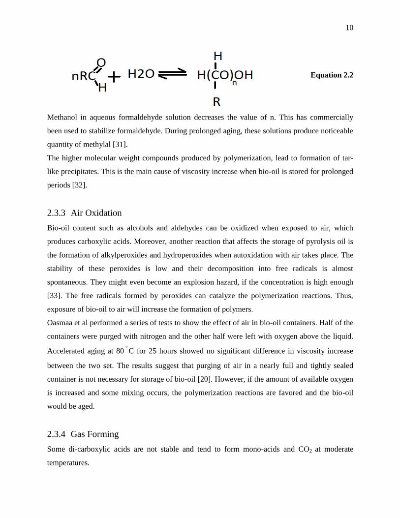
Equation 2.2 shows this reaction:
10
Equation 2.2
Methanol in aqueous formaldehyde solution decreases the value of n. This has commercially
been used to stabilize formaldehyde. During prolonged aging, these solutions produce noticeable
quantity of methylal [31].
The higher molecular weight compounds produced by polymerization, lead to formation of tar-
like precipitates. This is the main cause of viscosity increase when bio-oil is stored for prolonged
periods [32].
2.3.3 Air Oxidation
Bio-oil content such as alcohols and aldehydes can be oxidized when exposed to air, which
produces carboxylic acids. Moreover, another reaction that affects the storage of pyrolysis oil is
the formation of alkylperoxides and hydroperoxides when autoxidation with air takes place. The
stability of these peroxides is low and their decomposition into free radicals is almost
spontaneous. They might even become an explosion hazard, if the concentration is high enough
[33]. The free radicals formed by peroxides can catalyze the polymerization reactions. Thus,
exposure of bio-oil to air will increase the formation of polymers.
Oasmaa et al performed a series of tests to show the effect of air in bio-oil containers. Half of the
containers were purged with nitrogen and the other half were left with oxygen above the liquid.
Accelerated aging at 80 C for 25 hours showed no significant difference in viscosity increase
between the two set. The results suggest that purging of air in a nearly full and tightly sealed
container is not necessary for storage of bio-oil [20]. However, if the amount of available oxygen
is increased and some mixing occurs, the polymerization reactions are favored and the bio-oil
would be aged.
2.3.4 Gas Forming
Some di-carboxylic acids are not stable and tend to form mono-acids and CO2 at moderate
temperatures.

11
Equation 2.3 shows this reaction:
Equation 2.3
Where R & R’ could be hydrogen or alkyl groups. For example if both R & R’ are H, the
reaction proceeds at 150
C [34]. In addition, keto-acids form ketone and CO2 at low
temperatures.
Equation 2.4 demonstrates this path:
Equation 2.4
If R is –CH3 group, the reaction takes place readily at 25 C [34].
The other CO2 forming path in bio-oil is from ferulic acid, which is mainly due to the presence
of lignin in pyrolysis process. Equation 2.5 explains this reaction:
Equation 2.5
It has been observed that single carbon-carbon bond has lower breakage activation energy than a
normal bond and in the presence of oxygen, the decomposition rate is much more rapid which
introduces the idea of free radicals being involved. The free radicals that are present in the
aqueous phase of bio-oil can catalyze this reaction at low storage temperatures [35].
Peacocke et al analyzed the headspace of a bio-oil container which was sealed and stored for 6
months at ambient temperature. The gas in the positive pressure build up headspace was run
through a GC and contained 29 vol % CO2, 1% CO, 1% CH4, 61% N2, and 6% O2. It can be
assumed that all nitrogen was from the trapped air and the 10% missing oxygen could have

12
contributed to about 10% of 29% CO2, the rest of the oxygen present in CO2 coming from the
oxygenated compounds [36].
2.4 Effects of aging on bio-oil properties
2.4.1 Visual & Structural Changes
Oasmaa reported the visual changes in one month stored bio-oil as a change in colour from
reddish-brown to dark brown and an increase in dimness of the liquid. Formation of some flaky
sediments occurred after a few months of storage at 9 C [37].
Garcia-Perez et al. analyzed the structural changes that take place during aging. Figure 2.4 shows
cross-polarized pictures, taken at 30 C, of bio-oil at different aging times. The aging process was
accelerated by exposing the sample to 80 C.
Figure 2.4 – Changes of Waxy material morphology during Aging [38]
It is observed that the morphology of waxy materials change with time, suggesting
polymerization reactions happening between these materials and formation of new crystal
structures [38].

13
2.4.2 Viscosity
There are several literatures that suggest the viscosity of bio-oil increases with time of aging. Yu
et al. analyzed the aging of microwave pyrolysis liquid of corn stover and showed that
accelerated aging of bio-oil at 60 C would result in a rapid increase in viscosity of pure (original)
bio-oil. Adding a solvent would decrease both the viscosity and rate of viscosity increase,
however there is still an increasing trend with time. Figure 2.5 demonstrates all these information
graphically [39].
Figure 2.5 - Viscosity of bio-oils and bio-oils with solvent addition at 60°C [39]
Boucher et al conducted a study on bio-oil obtained from vacuum pyrolysis of softwood bark.
They measured the viscosity of different samples aged at 40, 50 and 80 C for 1, 6, 24 and 168
hours. They also found that viscosity of the bio-oil grows as the time of heating increases. In
addition, higher temperature of heating causes greater increase in viscosity. Figure 2.6 presents
the viscosity data for bio-oil aged at 80 C, measured at 30
C [40].
Chaala et al. considered the natural aging of vacuum pyrolysis liquid of softwood bark at room
temperature. Their result showed the same trend, however they also demonstrated that viscosity
of the bio-oil decreases at each point in time if the temperature is increased. Figure 2.7 presents
this information. The viscosity increase rate was also calculated for accelerated aging tests,
assuming a linear relationship between the viscosity and heating time. The data suggests that bio-

14
oil experiences a rate of increase in viscosity when heated at 80 C that is almost an order of
magnitude larger than when bio-oil is heated at 60
C. This information suggest strong
temperature dependence for aging [25].
Figure 2.6 – Viscosity of bio-oil from softwood bark aged at 80 C [40]
Figure 2.7 – Effect of Storage Time and Measurement Temperature on Viscosity [25]
Oasmaa and Kuoppala studied one year storage of forestry residue pyrolysis liquid at room
temperature in tightly sealed glass containers. The increase in viscosity over time is observed
here as well. In addition, the results indicate that the rate of increase in viscosity diminishes after
the first month, and starts to retard significantly after 6 months. Figure 2.8 depicts this
observation, as the time of storage becomes greater, the slope of the tangent (k) decreases [37].
0
100
200
300
400
0 50 100 150 200
Viscosity (cSt)
Aging Time (h)
heated at 80 C

15
Figure 2.8 – Rate of viscosity increase vs. time of storage [37]
2.4.3 Water Content
As mentioned earlier, the by-product of the main reactions occurring during aging is water.
Therefore, an increase in the amount of water present in bio-oil is expected over time.
Yu et al. performed accelerated aging experiments at 60 C on bio-oil from corn stover and their
results showed an increase in water content for pure (original) bio-oil. It is also understood from
the data that addition of solvents would both decrease the water content of bio-oil and slow the
water concentration increase. The results are summarized in Figure 2.9 [39].
Figure 2.9 – Effect of Aging and Solvent Addition on Water Content [39]
Czernik et al. also found that water content of the bio-oil increases with time. This increase was
greater and faster when bio-oil was stored at a higher temperature. Their data is presented in
Table 2.1 [27].

16
Table 2.1 – Effect of Aging Time and Temperature on Water Content [27]
37 C 60
C 90
C
Time (Days) Water (wt%) Time (Days) Water (wt%) Time (Days) Water (wt%)
0 16.1 0 16.3 0 16.2
7 16.2 1 16.3 1 16.2
17 16.6 2 16.6 2 16.6
28 16.5 3 17.1 4.5 17.3
56 16.6 6.7 17.7 8 17.5
84 16.6 9 17.7 15 17.7
Diebold and Czernik studied the effect of water content on the aging rate of bio-oil. Figure 2.10
shows that increasing the water content from 20% to 25% slows down the aging rate by almost
16% [32]. This could be an explanation for the previous result on increasing water content over
time flattening out after a certain time. As more water is produced over time, the aging rate is
slowed which in turn reduces the production of water. The addition of methanol also decreases
the aging rate.
Figure 2.10 – Effect of Water Content and Methanol on Aging Rate [32]

17
2.4.4 Average Molecular Weight
Oasmaa and Kuoppala suggest that there is a direct correlation between average molecular
weight of bio-oil and its viscosity. Therefore, they showed that over time the average molecular
weight of bio-oil increases which is the reason for the viscosity increase. Figure 2.11 presents the
changes in constituents of bio-oil over time when stored in sealed glass containers at 9 C. It can
be seen that the only components with major changes are ether-soluble (ES) materials and High
Molecular Weight (HMW) lignin materials which are the dichloromethane-insoluble fraction of
water-insolubles. Ether-solubles decreased gradually over time, mainly in aldehyde and ketones.
The oxygen content of ES decreased and that of Low Molecular Weight (LMW) lignin
increased. However, since the amount of LMW did not change significantly, some of it might
have converted to HMW lignin fraction [37].
Figure 2.11 – Effect of Aging on Bio-oil Constituents [37]
Czernik et al. performed measurements on naturally and accelerated aged samples of bio-oil and
realized that the proportion of the low molecular weight material decrease over time while that of
high molecular weight material increased. Table 2.2 presents the data that shows an increase in
average molecular weight for stored bio-oil [27].

18
Table 2.2 – Effect of Aging on Average Molecular Weight of Bio-oil [27]
37 C 60
C 90
C
Time
(Days)
Molecular
Weight
Time
(Days)
Molecular
Weight
Time
(Days)
Molecular
Weight
0 530 0 530 0 530
7 540 1 610 1 560
17 580 2 680 2 600
28 630 3 730 4.5 690
56 690 6.7 860 8 790
84 730 9 890 15 880
Chaala et al. divided the molecular weight range of compounds present in bio-oil into categories
and analyzed each category. Figure 2.12 shows a decrease in the fraction of lower molecular
weight compounds while the fraction of higher molecular weight materials increases with the
heating time at 80 C. This translates into an increase in average molecular weight of bio-oil with
time of storage [25].

19
Figure 2.12 – Effect of Aging on Different Molecular Weight Compounds [25]
2.4.5 Volatility
Thermogravimetric analysis (TGA) under nitrogen performed on fresh bio-oil and heat treated
bio-oil for 168 hours at 80 C in a sealed container, shows a loss in volatility and an increase in
the non-evaporative residue. Figure 2.13 demonstrates the effect of aging on the volatility of bio-
oil and the residue [25].
It is obvious that if the aging happens in a container that is not properly sealed, almost all the
volatile material of bio-oil will be lost and a thick, viscous tar-like material will be left.
Figure 2.13 – Effect of Aging on Volatility [25]

20
2.4.6 Phase Separation
The reasons for phase separation are substantial polarity, density and solubility difference
between the hydrophobic extractives and hydrophilic compounds present in bio-oil [28].
Yu et al. performed aging tests on bio-oil from microwave pyrolysis of corn stover and reported
phase separation. A water-rich layer appeared on the top and a tar-rich layer appeared on the
bottom after 30 days at 40 C and 15 days at 60
C. When solvent (methanol or ethanol) was
added to bio-oil, no phase separation was observed after 30 days at both 40 C and 60
C. This
suggests that solvent addition has another benefit which is prohibiting the bio-oil from phase
separation. This is especially valuable for bio-oil storage [39].
2.5 Methods to Slow Down Aging
Aging has a negative effect on the fuel quality of bio-oil and hence preventing it or at least
slowing down the process has potential advantages for both manufacturers and end users. The
usual methods involve solvent addition, mild hydrogenation to reduce the inherent oxygenated
compounds and proper sealing to minimize the exposure to air.
2.5.1 Solvent Addition
One of the earliest recommendations to add water, methanol or acetone to pyrolysis oils was
made by Polk and Phingbodhippakkiya. However, they did not present any data to illustrate the
usefulness of solvent addition to prohibit some the chemical reactions and avoid large increase in
viscosity [41].
Water addition effects analysis show that increasing the water content from 17 wt% to 30 wt%
reduces the bio-oil viscosity measured at 25 C from 1127cP to 199 cP. Moreover, the rate of bio-
oil aging after 4 months of storage at room temperature with 20 wt% water was 3.3 cP/Day. This
value was decreased when water was added to reach 25 wt% and 30 wt% to lower rates of 0.9
cP/Day and 0.05 cP/Day, respectively [42].
The effect of ethanol addition was investigated by Oasmaa et al. Ethanol was added to hardwood
bio-oil at 2 wt%, 5 wt%, 10 wt% and 20 wt%. The samples were aged for 4 months and the rate
of the viscosity increase was measured. The sample with no ethanol added showed an increase

21
with a rate of 0.12 cSt/Day, while the sample with 20% ethanol experienced only a minute aging
rate of 0.01 cSt/Day. Accelerated aging tests were also performed. Bio-oil was aged for 7 days at
50 C and the rate of viscosity increase reduced from 3.5 cSt/Day for pure bio-oil to 0.4 cSt/Day
for the mixture of bio-oil and 5 wt% ethanol [20].
Diebold and Czernik investigated the influence of different solvents on the aging rate of bio-oil.
As much as 10 wt% solvent was added including methanol, ethanol, acetone, ethyl acetate, 50/50
mixture of methanol and acetone and a 50/50 mixture of methyl iso-butyl ketone and methanol.
The experiments were carried out by accelerated aging of bio-oil at 90
C. The variation of
viscosities of pure bio-oil and the mixtures with time proved to be somewhat linear. The pure
bio-oil exhibited a rate of 60 cP/Day of viscosity increase. This value was reduced to 12 cP/Day
and 3.4 cP/day when 5 wt% and 10 wt% methanol was added, respectively. The samples with 10
wt% ethyl acetate, ethanol and acetone, measured a viscosity change rate of 8.6 cP/Day, 5.3
cP/Day and 4.6 cP/Day, respectively. The rate of increase in viscosity of the mixture of 5%
methanol and 5% methyl iso-butyl ketone was 6 cP/Day and the other mixture of 5% methanol
and 5% acetone was 4.8 cP/Day. Methanol proved to be the most promising of these solvents
because of both its lower price and effectiveness in slowing the aging process [32]. Figure 2.14
summarizes all these changes over time.

22
Figure 2.14 – Effects of additives on aging [32]
The timing of the solvent addition was demonstrated to be an important factor as well. Diebold
and Czernik used accelerated aging method to age two samples for 20.5 hours at 90 C. The first
one was pure bio-oil and the second one contained a mixture of bio-oil and 10 wt% methanol.
The viscosities of the sample measured at 40 C were 80 cP and 17 cP. After these measurements,
10 wt% methanol was added to aged pure bio-oil to recover its viscosity, however it only got
reduced to 25 cP. This observation suggests that adding solvents right after bio-oil production is
the best way to prevent it from aging; however storage volume might become an issue [32]. It
has also been mentioned elsewhere that a mixture of fresh bio-oil and 5 wt% methanol showed a
15% increase in viscosity when stored for 3 months at room temperature, while the same bio-oil
aged at the same condition and added the same amount of methanol after the storage time
experienced a viscosity increase at about 28% [33].
2.5.2 Very mild hydrogenation
Hydrogenation has been used in unsaturated vegetable oils to make it stable. The result is a
greasy semisolid material used sometimes instead of butter. However, this increase in viscosity is

23
not desirable for bio-oil fuel applications although the process would saturate the reactive
compounds and slow the aging of bio-oil.
A hydrogenation study was performed on bio-oil with a Palladium catalyst on carbon. After 8
months of aging at room temperature, the viscosity of the bio-oil diluted with 20% m-cresol
increase 72%, while the diluted hydrogenated bio-oil experienced only 21% increase in viscosity.
However, adding the solvent suggests that the viscosity increase after hydrogenation has been
significant although no data has been provided on the actual value [41].
2.5.3 Minimizing the exposure to air
As previously mentioned, the minor volume of air trapped on top of the bio-oil in a container
does not have any major effect on aging. However, if more air is available to the bio-oil, the
outcomes might not be the same. Mixing bio-oil with a medium to high speed blender in an open
container would result in bubble formation and the entrained air would saturate the bio-oil. This
augmented level of available oxygen could be responsible for production of peroxides that would
act as a catalyst for polymerization reactions. Limiting the access of air to bio-oil is necessary to
reduce the likelihood of peroxide formation that catalyzes the polymerization of olefins. Adding
some antioxidant such as hydroquinone also stabilizes the olefins, and seems to be more cost
effective than hydrogenation [33].
2.6 Droplet Combustion of Bio-oil
Bio-oil spray combustion can be explained with the aid of analysis on single droplet burning
studies. There are typically four stages in the droplet combustion of bio-oil: (1) surface burning
of volatiles, (2) droplet micro-explosion and a burst of fuel vapor, (3) sooty combustion of
micro-explosion droplets, (4) solid state combustion of the residues [43]. Figure 2.15 shows
these stages.

24
Figure 2.15 – Four Stages of Bio-oil Droplet Combustion (left to right) [43]
After ignition, evaporation of volatiles takes place from the surface of the droplet and a spherical
blue flame is produces by the quiescent combustion of these volatile compounds. During this
process, the outer crust is mostly left with viscous HMW material due to the loss of evaporative
compounds and the surface is exposed to heat and oxygen which leads to polymerization of these
heavier materials. This phenomenon causes the formation of a hardened shell on the surface of
the droplet which prevents the volatiles from escaping outside of the droplet [44]. As more
heating is provided to the droplet, more material evaporates inside the restricted shell and
pressure is build up there, leading eventually to a micro-explosion to take place. This micro-
explosion produces many more droplets with a reduced effective diameter. Right after this stage
that is recognized by a yellow flame attributed to soot burning, the droplet contracts to almost the
original diameter. This is accompanied by a reduction in flame size around the droplet, indicating
a substantial decrease in fuel evaporation. The last stage of droplet combustion begins when the
flame extinguishes completely [45]. The porous cenosphere left from the previous combustion
stages, burns in a non-volatile solid-state, fuel-rich combustion mode. The details of
heterogeneous burning of this carbonaceous residue are depicted in Figure 2.16. The non-
evaporative fraction of bio-oil that should be burned heterogeneously is usually about 20-30%.
At the end, the only material remaining should be ash, if complete combustion takes place [24].
Figure 2.16 – Solid State Combustion of the Cenospheric Residue [43]

25
Thermogravimetric analysis of bio-oil can also give insight to the combustion stages [24].
Although heating rates and time scales are totally different between TGA and droplet
combustion studies, the stages can be described similarly based on the results. TGA suggests that
very high temperatures and long residence time is required for complete burnout of carbonaceous
residue. This implies that bio-oil may not be well suited to combustion devices that require full
evaporation of the fuels such as internal combustion engines and jet engines.
2.7 Effect of Bio-oil Properties on Spray Combustion
2.7.1 Viscosity
Tzanetakis et al. have used a correlation to estimate the bio-oil droplet size or Sauter Mean
Diameter (SMD) coming out of an air-blast nozzle. One of the many parameters in this
correlation is the dynamic viscosity of bio-oil (µL). Equation 2.6 presents this correlation.
[
]
Equation 2.6
After performing spray combustion test with biooil-ethanol blends, they concluded that as the
calculated droplet size increases, the combustion quality becomes inferior and emissions rise.
This effect is shown in Figure 2.17 [7].

26
Figure 2.17 – Effect of SMD on Combustion [46]
As a result, one could conclude that since increasing viscosity tends to increase the droplet size,
it will deteriorate the combustion performance and increase the emissions.
2.7.2 TGA Residue
Thermogravimetric analysis provides insight on the fuel`s volatility. The TGA residue is a
measure of non-volatile matter present in the liquid. As this residue increases in bio-oil,
combustion becomes more challenging. Moloodi analyzed the effect of TGA residue on
combustion and emissions of bio-oil by adding different amounts of ethanol to bio-oil in order to
vary the TGA residue of the fuel. It was concluded that more volatile matter helps ignition and
sustainable combustion. This led to lower emission for the batch with lower TGA residue. The
effect of TGA residue on CO emission of bio-oil combustion is presented in Figure 2.18 [22].

27
Figure 2.18 – Effect of TGA Residue on Combustion [22]
2.7.3 Water Content
Water removal from bio-oil causes the adiabatic flame temperature to increase owing to higher
heating value, and droplet evaporation time to decrease due to the large latent heat of evaporation
of water [47]. Moreover, removing water increases the viscosity of bio-oil and lowers the
probability of having micro-explosions in droplet combustion [48].
Moloodi investigated the effect of water content on bio-oil spray combustion performance and
concluded that more water decreases the emission. Two batches of bio-oil with similar solids and
ash content and same ethanol addition were tested in a spray burner. The main difference was the
TGA residue because of water dilution. Figure 2.19 shows that emission decreases as water
content increases [22]. However, it needs to be mentioned that the water content of bio-oil has an
upper limit for combustion purposes. More water will decrease the heating value and rate of
combustion reactions, which in turn would cause instability and termination of combustion. In
addition, too much water would accelerate phase separation of bio-oil when stored.
0
200
400
600
800
1000
1200
1400
14% 15% 16% 17% 18%
CO
(P
PM
)
TGA Residue
CO

28
Figure 2.19 – Effect of Water Content on Combustion [22]
2.7.4 Solids & Ash Content
Effects of solids & ash content on combustion performance of bio-oil have been examined in the
literature [22]. To show the isolated effect of solids, three batches with similar ethanol addition,
water content and SMD were chosen. Author has labeled them S2, S3 & S4 with 0.089%,
0.839% and 2.217% solids content. Figure 2.20 shows that the emissions increase with
increasing solids content of the fuel. The large jump from S3 to S4 is mainly due to the almost
doubling of solids content as well as a substantial increase in char particle size which requires
more time for complete heterogeneous combustion [45]. The effect of ash is considered when
two batches with similar solids, water and ethanol content but different ash content were tested.
The first batch had 0.027% and the second batch had 0.223% ash, and the CO emissions were
202.9 ppm and 498.0 ppm, respectively. The increase in emission corresponding to an increase in
ash content may be due to catalytic effect of alkali metals in the gasification of char particles
[49].

29
Figure 2.20 – Effect of Solids Content on Combustion [22]
A linear correlation between carbonaceous residue emissions with the amount of solids content
and the TGA residue of the fuel has been suggested by Moloodi [22]. It shows that the effect of
the TGA residue is greater than the solids content.
0
200
400
600
800
1000
1200
1400
0.0% 0.5% 1.0% 1.5% 2.0% 2.5%
CO
[m
g/M
J]
Solids[%]
CO
S2 S3
S4
30
3. Experimental Methodology
3.1 Spray Burner
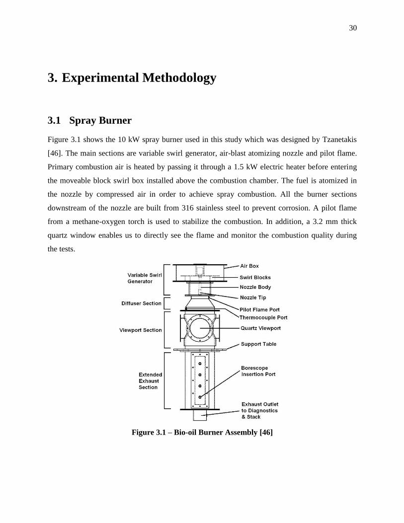
Figure 3.1 shows the 10 kW spray burner used in this study which was designed by Tzanetakis
[46]. The main sections are variable swirl generator, air-blast atomizing nozzle and pilot flame.
Primary combustion air is heated by passing it through a 1.5 kW electric heater before entering
the moveable block swirl box installed above the combustion chamber. The fuel is atomized in
the nozzle by compressed air in order to achieve spray combustion. All the burner sections
downstream of the nozzle are built from 316 stainless steel to prevent corrosion. A pilot flame
from a methane-oxygen torch is used to stabilize the combustion. In addition, a 3.2 mm thick
quartz window enables us to directly see the flame and monitor the combustion quality during
the tests.
Figure 3.1 – Bio-oil Burner Assembly [46]

31
3.1.1 Overall Setup
Figure 3.2 presents the schematic of the overall experimental system. The main inputs of the
burner are fuel and atomizing air through nozzle, primary combustion air and methane-oxygen
mixture for pilot flame. Two parallel peristaltic pumps are used to deliver ethanol or bio-
oil/ethanol mixture to the nozzle. All fuel lines are chosen from 316 stainless steel or Teflon
tubing for corrosion resistance. Fuel is atomized in the nozzle by compressed air that is passed
through a pressure regulator and rotameter. The primary combustion air is provided by a stack
fan downstream of all instruments in the system. The air is heated to between 250-300 C by a
heater mounted on top of combustion chamber and the flow is controlled by changing the voltage
on stack fan using a variac. The whole system operates at a slight negative pressure of 200-300
Pa provided by the stack fan in order to contain the exhaust gases and discharging them to the
roof stack and preventing them from spreading into the room.
Exhaust is cooled to room temperature using a spiral heat exchanger and most of particulate
matter is collected in the water traps below the heat exchanger. However before the heat
exchanger, a sample stream is tapped from the exhaust line downstream of combustion chamber
using a 6.4mm stainless steel heated line that avoids condensation. The sample passes through a
filter to remove PM before entering the gas phase emissions measurement instruments. PM is
also isokinetically sampled and collected on a filter for analysis. Details of gas phase and PM
emissions measurements will be discussed in the following sections.

32
Figure 3.2 – Overall schematic of experimental setup [46]
3.1.2 Variable Swirl Generator
Swirling flows introduce tangential velocity that causes angular momentum to the streamlines of
the main combustion air. The movable block swirl generator shown in Figure 3.3 can change the
ratio between axial and angular momentum of the flow by changing ζ [46]. The fixed swirl block
angle is represented by α and is set to 60 and the maximum operating angle shown by ζm is 12
.
If angular momentum is made large enough compared to axial momentum, a pressure gradient in
the opposite direction of the bulk flow is created. This causes the fluid to flow back toward the
upstream region, creating a central recirculation zone (CRZ) which is especially beneficial for
combustion systems in terms of mixing and stability. This concept is depicted in Figure 3.4.

33
Figure 3.3 – Schematic of Movable Block Swirl Generator [46]
Figure 3.4 - CRZ of swirling flows in confined geometry [50]
In swirling flows, the conservation of axial flux of momentum applies for both radial (GΦ) and
axial (Gx) directions [51]:
∫
Equation 3.1
∫
∫
Equation 3.2
where W, U and p are tangential and axial components of velocity and local static pressure,
respectively. Based on these parameters, the non-dimensional swirl number S is introduced,
which characterizes the ratio between angular and axial momentum fluxes and enables to

34
compare the swirl intensity of different flows. In order to obtain CRZ, a minimum swirl number
between 0.5 < S < 0.6 is required [50]. The movable block swirl generator used in this study is
capable of achieving S = 5.41 when swirl is set to 100%.
3.1.3 Air-Blast Atomizing Nozzle
An internal mix, air-blast nozzle from BEX Engineering Ltd. (model 1/4”JX6BPL11 with a 152
mm long extension tube and 2X2JPL back-connect body) is used in this study. The internal
construction and assembly of the nozzle is depicted in Figure 3.5. All the components are made
from stainless steel in order to avoid erosion and corrosion. The nozzle is placed along the
centerline of the burner and there is only 15.9 mm clearance between the tip of the nozzle and
the centerline of the pilot flame in order to spray the fuel-air mixture as close as possible to the
ignition source.
Figure 3.5 – Atomizing Nozzle Tip Assembly [52]
Fuel is carried through a 1.0 mm single liquid cap orifice to the internal mixing chamber, where
it is mixed with air. After that, the spray exits through six symmetrically spaced, 0.89 mm air cap
discharge orifices. The six individual jets make an angle of 60 with the centerline of the burner
and create a hollow cone pattern. This is important because the center of the spray does not
introduce any significant axial momentum along the centerline of the flow compared to central
discharge orifice. This benefits the formation of a CRZ that helps combustion stability.
Another factor that affects stability is fuel boiling. If this phenomenon is controlled for
atomization, it is called flash boiling atomization and it can benefit the combustion by reducing

35
the droplet size and widening the spray angle [53]. However, in the system used for this study,
the boiling and bubble forming causes instability which sometimes ends in flame blow-out.
Therefore, a water cooling system for the nozzle was designed by Moloodi in order to prevent
the fuel from boiling and avoid the instabilities. Figure 3.6 depicts the details of this cooling
system which consists of a 1/16” stainless steel tube enveloped helically around the nozzle body
[22]. Fuel temperature is monitored and whenever the boiling is about to happen, a ball valve is
manually opened to allow water to run through the system and cool down the fuel.
Figure 3.6 – Schematic of Nozzle Cooling System [22]
3.1.4 Pilot Flame
An oxy-fuel torch body and standard No. 7 tip with a 1.2 mm orifice diameter (Hoke Model No.
110-406) is inserted vertical to the axis of the burner to produce a fully premixed stoichiometric
methane-oxygen flame. The tip has a hexagonal slit which allows multiple flames to be issued
from the small openings, producing a wider overall flame. The energy throughput of the pilot
flame is 5% of the total 10 kW input from bio-oil blends, which corresponds to 0.88 standard
liters per minute (SLPM) of methane and 1.8 SLPM of oxygen. The pilot is always kept running
during a test, in order to sustain and stabilize the combustion.
Although the relative position of the pilot flame to the burner is fixed, nozzle orifices and the
pilot flame need to be aligned. The procedure is described by Tzanetakis [46]. Pure ethanol is
burnt in the combustion chamber and the nozzle is rotated until an evenly distributed spray flame
is observed and the pilot flame does not impinge on any of the fuel jets. Figure 3.7 describes the
difference between a good and poor alignment. After the correct configuration is found, the
nozzle is locked into place by four set-screws and won’t be repositioned unless a major nozzle
cleaning is required.

36
Figure 3.7 – Alignment of Pilot Flame [46]
3.2 Fuel Analysis
3.2.1 Fuel Composition & Heating Value
Fuel composition of the bio-oil is reported by measuring the carbon, hydrogen and nitrogen and
assuming that the rest is oxygen. The solids, ash and water content of the fuel are also important
for analyzing and predicting the behaviour of the combustion. The higher heating value (HHV)
needs to be determined in order to calculate the flow rate required for a 10 kW operation.
Table 3.1 lists the measurement methods used to obtain these properties which are outsourced for
measurements.
Table 3.1 – Fuel properties measurement standards
Property Test Method
Water Content ASTM E203
Solids Content MeOH-DCM insoluble
Ash Content ASTM 482
C-H-N-O ASTM 5291
HHV ASTM 4809

37
3.2.2 Viscosity
Viscosity has an effect on atomization quality and pumping of liquid fuels. The viscosity of pure
bio-oil was measured at room temperature using a handheld dip viscometer (Zahn Cup) before
each combustion test. The time required for the liquid to be drained from the cup is recorded and
using a correlation provided by the manufacturer, the time is converted to viscosity. This
measurement method is used 3 times for each sample and the arithmetic average is presented as
the data. However, the result is not very accurate and is only used for comparison between
different samples. More accurate measurement is outsourced to be done according to standard
ASTM D445 at 40 C for pure bio-oil and 80
C for bio-oil/ethanol blend which is closer to the
fuel temperatures exiting the spray nozzle. This measurement method uses a calibrated glass
capillary tube and is suitable for opaque fluids. For the higher temperature, slow heating rate is
required to avoid bubble formation from evaporation of volatiles in order to achieve more
accurate results [54].
3.2.3 Thermogravimetric Analysis
Two important pieces of information are obtained when TG analysis is performed: fuel’s
volatility distribution and its tendency for formation of a solid residue [44]. For this study, a TA
Instrument Q50 Analyzer is used. The bio-oil and ethanol blend is shaken to achieve a
thoroughly mixed and homogenized fluid. Then, a 15-20 mg sample is picked and placed on an
aluminum pan, which is put on the sample holder of the TG analyzer. Throughout the test, the
sample is kept under a 100 ml/min atmospheric flow of nitrogen. Heating starts at a rate of 10
C/min after 5 minutes of running nitrogen through the lines in order to deplete the system from
any Oxygen. The heating continues for an hour to reach a maximum temperature of 600 C. The
percentage of the material left at the end of the test is a representative of fuel’s tendency for char
formation and is named as “TGA residue” hereafter.

38
3.3 Gas Phase Emissions Measurement
Exhaust emissions were analyzed for carbon monoxide (CO), nitrogen oxides (NOx), unburned
hydrocarbons (UHC) and oxygen (O2) percent. Different instruments have been used for
measurement, which have been described in detail elsewhere [46]. The schematic of sampling
and analysis system is depicted in Figure 3.8. All the sampling lines and chambers are heated via
either heated tapes or feedback controlled heaters, and the temperature of the gas is maintained at
190-195 C in order to avoid any condensation in the lines.
Figure 3.8 – Schematic of the gas phase emissions measurement system [46]
3.3.1 Oxygen Concentration
The fraction of the exhaust that is composed of oxygen can be determined continuously using a
Zirconia (ZrO2) model OXY6200 oxygen sensor. The accuracy of this sensor is ±0.1 %O2 and it
is calibrated by running ambient room air through it to set the 21 vol% mark. The output is a 0-5
VDC that is linearly proportional to the 21% concentration. A stream of exhaust sample is passed
through the oxygen sensor at a flow rate of 1.8 SLPM provided by a vacuum pump. A separate
sampling line is used for this sensor as seen in Figure 3.8, because it operates at a high

39
temperature which can oxidize hydrocarbons and CO of the exhaust and affect the detection
results.
The voltage output of the sensor is logged by a data acquisition system and is used to back
calculate the equivalence ratio of the combustion. The voltage is translated into the percent
oxygen in exhaust, and by using the fuel’s atomic composition from CHNO analysis and
assuming complete combustion, real-time equivalence ratio and the flow of primary combustion
air required for that equivalence ratio is calculated. Since, the amount of CO present in exhaust is
in most cases below 0.2%, the complete combustion assumption only has minor effect on the
results and the error can be neglected.
3.3.2 Unburned Hydrocarbons
Unburned Hydrocarbon (UHC) emissions are measured using a flame ionization detector (FID)
from California Analytical Instrument. The detection mechanism of this device is that a sample
of exhaust is passed through a small hydrogen flame which produces a current proportional to
the number of carbon atoms in the sample [55]. The flow rate of this sample is automatically
kept at 1.5 SLPM by an internally built vacuum pump. The temperature of this exhaust sample is
kept at 190-195 C to prevent the heavier hydrocarbons from condensing. The current produced
by the flame is outputted as a voltage of 0-5 VDC and is fed into a data acquisition system
connected to a computer. Before each combustion test, the FID is calibrated by setting two
values. The first one is zero, using purified air and the second point is set to 90.2 ppm of methane
in air. The range is extrapolated to a maximum of 300 ppm with an uncertainty of ±3 ppm.
3.3.3 Detailed Speciation of Pollutants
The concentration of carbon monoxide (CO), NOx, methane (CH4), formaldehyde (CH2O),
acetaldehyde (C2H4O), carbon dioxide (CO2) and water (H2O) emissions in the exhaust sample
are measured using a Nicolet 380 Fourier Transform Infrared Spectrometer (FTIR). This
spectrometer compares the absorption spectrum of a gas sample in the mid infrared region (500
to 4000 cm-1
) against known standards [56].

40
A two way valve is used to switch the gas sampling between FID & FTIR. The FTIR gas cell has
a sample volume of 0.19 L and gas is continuously drawn into it at a flow rate of 10.3 SLPM and
a pressure of 86.3 kPa when spectra are taken. Each spectrum is obtained by scanning the sample
24 times over 1 minute at a resolution of 1 cm-1
, which translates into about 50 refills of the gas
cell per spectrum. A total of 5 spectra are taken for each combustion test and the arithmetic
average of the measured emission values are presented.
The calibration is done via a partial least square model using different gas mixtures of the
compounds considered in the study. Details of the FTIR calibration experimental setup and
method are provided in a previous work [57]. The minimum concentration of each species that
outputs a signal to noise ratio of 4 is set as the detection limit. The root mean square error
(RMSE) determines how accurate the model is by representing the deviation between the
predicted value by the model and actual concentration of the employed standard gas sample
mixture. Table 3.2 summarizes the detection limits and the accuracy of the models. Two separate
models have been used in this study, corresponding to different ranges of CO concentration. This
is due to the nonlinearity of CO absorption versus concentration curve. Each spectrum is
compared with the standard gas spectra to determine which of the two models is more suitable
for quantifying the spectrum.
Table 3.2 – Detection limits and uncertainty levels of the
FTIR calibration model
Species Units Detection Limits RMSE
CO (Low) ppm 10-600 15.6
CO (High) ppm 600-1500 25.5
NOx ppm 10-300 6.3
CH4 ppm 10-250 3.1
CH2O ppm 10-150 1.7
C2H4O ppm 30-150 5.2
CO2 % vol 2-15 0.19
H2O % vol 0.5-15 0.12

41
3.4 Particulate Matter Emissions Measurement
There are two main factors involved in PM measurements of an exhaust stream. First, a sample
that accurately represents the exhaust PM needs to be obtained. Isokinetic sampling is the
method used in this study. Second, the sample has to be analyzed and the concentration of the
PM should be measured. For this matter, gravimetric analysis and loss on ignition methods have
been employed.
3.4.1 Isokinetic Sampling System
PM sampling of an exhaust stream is usually done by inserting a small diameter probe with an
opening that faces upstream in a way that minimum disturbance is imposed on the flow. Under
frictionless flow conditions, isokinetic velocities are achievable when gas enters the tube without
changing velocity [58]. In other words, isokinetic condition is obtained if the sampling nozzle is
set parallel to the flow stream and the suction velocity of the nozzle is equal to the exhaust gas
velocity [59]. It is important to satisfy the isokinetic sampling conditions because it provides an
unbiased size distribution of exhaust PM. Controlling the sampling flow rate via a needle valve is
the most common method of practice for ensuring closest approximation to isokinetic sampling.
Inertial effects make the larger and heavier particles deviate more from the gas streamline, while
smaller and lighter particles follow the streamline closely. Figure 3.9 shows that when the
exhaust flow velocity is more than the sampling velocity, flow streamlines tend to deflect
outwards when they encounter the nozzle. As discussed above, heavier particle don’t follow the
streamlines and tend to continue on their straight path through the nozzle. This phenomenon
results in a change in distribution of particle size in a way that larger particles of the flow get
accumulated on the filter and the sample will not be an accurate representative of the flow [60].

42
Figure 3.9 – Gas Streamlines around sampling probe (VS < V)
In order to find the sampling flow rate for isokinetic sampling condition, two methods are
recommended. First method is using a pitot tube to measure the gas velocity as described by
EPA [61]. The other method, called “null method”, matches the velocities of main stream and
sampling stream by matching their static pressure [58]. In this study, the pitot tube method was
not used due to large amount and size of PM which would have ended in clogging of opening
hole of the tube that faces upstream. As an alternative, the null method with two static pressure
measurement openings parallel to the streamlines was used. If Bernoulli’s equation is used along
a streamline that enters the probe, assuming the gas is incompressible and frictionless (Mach
number << 0.3), it can be shown that the velocities inside the sampling tube and the exhaust
streamline are the same when the static pressure difference at these points is zero.
In reality, friction of the gas and incompressibility effects can cause a deviation from the
assumptions made for isokinetic conditions. Therefore, a calibration method is required to
validate the accuracy of these conditions based on theoretical considerations. Some of these
details are briefly discussed in Appendix A. The outcome of these calculations is that the ideal
isokinetic sampling flow rate is determined to be 10.4 % of the total exhaust flow rate.
Figure 3.10 shows the schematic of the isokinetic PM sampling system. The gas mixture inside
the combustion chamber is highly swirling. Therefore, the angular momentum of the flow can be
seen far downstream of the swirl generator [62]. This causes non-uniformity in PM distribution

43
as particles tend to accumulate near walls. For solving this issue, a flow straightener is placed in
the outlet pipe of the burner. It is constructed of 0.25 mm thick stainless steel sheet metal
arranged into a 24 x 24 mm “checkerboard” pattern. The purpose of the flow straightener is to
ensure an axial pipe flow velocity profile is achieved and the PM distribution is uniform before
entering the isokinetic sampling probe.
The isokinetic sampling probe uses the pressure gradient between fully stagnated and free stream
flow, so the dynamic pressure inside the main exhaust pipe needs to be detectable. For this
matter, a pipe size reduction is placed in the system from the 102 mm i.d. elbow to 38 mm i.d.
elbow. This change in diameter causes the gas velocity to increase, which in turn, increases the
dynamic pressure to about 21 Pa. This pressure can be readily detected by a manometer with an
accuracy of 1.2 Pa. This manometer is used during the combustion tests to make sure the
pressure difference between the two streams is always zero by controlling the flow rate.
The sampling probe is placed in a way that flow disturbances such as bends and size reductions
have minimum effect on uniformity of PM distribution within the gas. It is recommended in
literature that the probe should be located 8-10 duct diameters downstream and 3-5 diameters
upstream of any disturbance in order to minimize the effect [63]. In the system used for this
study, the probe is positioned 10.4 diameters (394 mm) downstream of the elbow and 1.7
diameters (64 mm) upstream of any flow disturbance due the lab space restrictions.

44
Figure 3.10 – Schematic of PM sampling system [46]
Figure 3.11 shows the geometry and position of the sampling probe and the static pressure taps.
The sampling probe is made of 11.3 mm i.d., 12.7 mm o.d. seamless stainless steel tube. The
diameter size was selected based on recommendations made by EPA [61]. Some other
considerations included the maximum flow rate in the probe that the vacuum pump could sustain
during sampling time and a reasonable amount of PM mass collected on the filter during the time
that pump could draw flow. For this matter, 5 minutes of sampling was chosen in order to
optimize both requirements. In addition, small diameter tubes were inserted in the sampling tube
and mounted perpendicular to the exhaust stream, in order to measure the static pressure at these
points.

45
Figure 3.11 – Geometry and position of sampling probe and pressure taps [46]
The temperature of the gas running through the sampling probe is about 250 C, which would
damage some of the gaskets in the assembly. For this reason, gas temperature fed into the filter is
controlled to be between 120-130 C according to EPA methods [61]. To do so, a cooling jacket
that uses compressed air at room temperature surrounds the sampling tube as seen in Figure 3.10.
In addition to the main sampling line and filter, an auxiliary line and filter is installed with ball
valves required to switch the gas between them. This auxiliary line is used during a filter change
in the main line; the purpose is to keep the sampled gas flow at a steady rate. This switching
prevents any changes in the combustion chamber pressure and also keeps the sampling line
passages warm.
A 47 mm diameter Tissuquartz filter (Product No. 7221) provided by Pall Life Sciences is placed
in an Advantec MFS Inc. stainless steel filter holder body (Model LS47, Part No. 304700), in
order to collect exhaust PM. The filters are made of quartz fibers which can endure high
temperatures in the range of 1100 C without decomposing. They have a 99.9 % aerosol retention
efficiency for 0.3 micron diameter particles (measured by ASTM D2986-95A) [64]. As shown in
Figure 3.10, a J-type thermocouple with a 1.6 mm diameter stainless steel sheath measures the
gas temperature just downstream of the filter. In addition, a shut-off ball valve is located prior to
the holder body on both the main and auxiliary lines, in order to make a sudden start/stop in the

46
flow and accurately time the sampling process. When the valves are fully open, the diameter
matches the sampling line in order to minimize any obstruction and PM loss.
A shell and tube heat exchanger provided by Seakamp Engineering Inc. (Part No. 2151414), is
placed between filter holder bodies and the sampling pump to condense the water vapor and
prevent liquid accumulation inside the line and the pump. Water is run in the tubes to cool down
the exhaust gas that runs in the shell. The flow rate of water is about 0.25 GPM and the
temperature increase is about 2 C for all tests. In order to calculate the PM concentration, the
total flow rate through the sampling line should be quantified. However, the gas rotameter which
is calibrated at the test pressure, measures the “dry” exhaust flow rate. It cannot be used to
measure the flow rate before the heat exchanger because of condensation problems. These two
flow rates show a relationship when it is assumed that the gas coming out of the condenser is at
equilibrium and saturated with water vapour. By performing a mass balance over the condenser,
the following equation is found between the standard volumetric gas flow rates:
⁄
Equation 3.3
where Psat is the saturation pressure at the temperature of the gas exiting the condenser, Ptotal is
the absolute pressure as measured by the gauge in the condenser exit and Xwater vapor is the molar
fraction of water in the exhaust before heat exchanger, based on mixture stoichiometry calculated
from oxygen sensor.
3.4.2 Gravimetric & Loss on Ignition Analysis
There are two successive sampling filters for each bio-oil test. Each collection on a filter takes 5
minutes. Depending on the pressure drop over the filter, this time might change. For high PM
loading, 3 minutes is used and for depositions that has minimum effect on pressure and might be
detectable, 10 minutes of collection is used.
The filters are desiccated and cleaned from any contamination prior to each combustion test, by
placing them in an oven at 750
C for two hours. They are then weighed 3 times using a
Scientech SM-128D Microbalance, and placed in a Petri dish and caped. In order to calculate the
amount of unburned carbonaceous residue (CR) and ash of the PM, a standard method called loss

47
on ignition described by ASTM code number D4422-03 was followed for each of the filters after
combustion tests [65]. The filter is placed in the Petri dish and capped immediately after
collecting it from the filter holder body. After the test, the collected filter is weighed 3 times
again to measure the total amount of PM. There is a high vapor content in the exhaust which gets
accumulated on the porous filter. A drying stage is done by placing the filter in the oven at 150 C
for two hours. Once more, the filter is weighed and the mass difference between this stage and
previous one, measures the water content present on the filter. Lastly, the filter is positioned in
the oven for an hour at 750 C for burning the CR fraction of the PM. The weight of the filter
containing only ash is measured 3 times. All the weights that are used for calculation are the
arithmetic average of the 3 measurements. Figure 3.12 shows these steps and Table 3.3 provides
the calculation method for each fraction of the PM based on the nomenclature of Figure 3.12.
Figure 3.12 – Gravimetric analysis and Loss on ignition procedure [22]
Table 3.3 – Calculation methods of each PM
fraction
Total PM(mg) M2 - M1
Water(mg) M2 – M3
CR(mg) M3 – M4
Ash(mg) Total-Water-CR

48
3.5 Flame Visualization
Combustion quality is evaluated by observing the flame through the viewport, monitoring
pressure fluctuations in the combustion chamber and using a borescope assembly to take pictures
and videos of the flame. These photographs qualitatively describe the trends in mixing and
atomization quality for each test.
Figure 3.13 shows a schematic of the flame visualization system used in this study. The probe is
a 9 mm diameter Lenox Instrument Co. direct view borescope with a tube length of 35 mm. It is
a rigid fiber-optic member that has a 90 angle mirror integrated to its body at one end and is
coupled to a 10 mega pixel camera at the other end. The mirror, when inserted in the burner,
provides an unobstructed, upward-looking view of the flame along the central axis of the burner.
In order to avoid very high temperatures on the optics, the optical assembly can be easily
inserted and removed from the burner via a rail-guide system. A 19 mm insulated tube surrounds
the fiber optic and lets compressed air at a flow rate of 250 SLPM pass through it, in order to
cool the optics and protect the mirror from PM impingement. This extra air is introduced far
downstream of the flame and in order to compensate for the fluid dynamic effects, stack fan
draw is increased until the same burner pressure as before these changes is achieved.
Figure 3.13 – Borescope Assembly [46]
During a combustion test, the probe is inserted through a tube fitting and remains there for only
5-10 seconds to a take a photograph or a short video. Several photographs are taken for each test

49
while the aperture opening (f-stop), shutter speed and ISO value (light sensitivity) of the camera
are manually adjusted to achieve the best picture quality possible. No post process image
treatment (besides cropping and resizing) is applied to any of the photographs.
3.6 Aging Procedure
For the purpose of this study, two separate batches of bio-oil have been used. Although
manufactured by the same provider and from the same feedstock, they had slightly different
properties and characteristics. First batch was poured into several bottles and sealed with a
plastic cap and separated into two categories. Some of the sealed bottles were stored in a
ventilated cabinet located in a room with a central climate control system which kept the
temperature at around 20 C. The cabinet’s door was kept closed and only opened when
temperature measurements were done, in order to keep the bio-oil out of any direct lighting. This
procedure is referred to as “Natural Aging” in this study, because the temperature is a close
approximate of room temperature. Figure 3.14 demonstrates the temperature fluctuations
measured on the glassware with a type K thermocouple over the period of the storage. The
frequency of the measurements was higher at the beginning to ensure consistency over different
times of the day.

50
Figure 3.14 – Temperature vs Time for Natural Aging
The rest of the bottles were stored in a fridge at 5 C, in order to slow down the aging of bio-oil to
a point that for the purpose of this study, it was considered no changes associated to aging
occurred during this storage. These bottles were taken out one by one from the fridge and placed
in a fume hood for five hours to reach the room temperature before “accelerated aging”
procedure could begin. In order to a mimic the natural aging in a shorter period of time, literature
has suggested that bio-oil can be heated up to higher temperatures and equivalent changes in
viscosity and average molecular weight are achieved after some time. A correlation is provided
by Diebold and Czernik for the aging rate as a function of temperature:
(
)
Equation 3.4 [32]
The aging rate here is defined as the change in viscosity over time and has a unit of cP/day and T
is the storage temperature in kelvin [32]. In order to calculate the time required to heat the bio-oil
0.0
5.0
10.0
15.0
20.0
25.0
30.0
05
/08
/20
11
0:0
01
5/0
8/2
01
1 0
:00
25
/08
/20
11
0:0
00
4/0
9/2
01
1 0
:00
14
/09
/20
11
0:0
02
4/0
9/2
01
1 0
:00
04
/10
/20
11
0:0
01
4/1
0/2
01
1 0
:00
24
/10
/20
11
0:0
00
3/1
1/2
01
1 0
:00
13
/11
/20
11
0:0
02
3/1
1/2
01
1 0
:00
03
/12
/20
11
0:0
01
3/1
2/2
01
1 0
:00
23
/12
/20
11
0:0
00
2/0
1/2
01
2 0
:00
12
/01
/20
12
0:0
02
2/0
1/2
01
2 0
:00
01
/02
/20
12
0:0
01
1/0
2/2
01
2 0
:00
21
/02
/20
12
0:0
00
2/0
3/2
01
2 0
:00
12
/03
/20
12
0:0
02
2/0
3/2
01
2 0
:00
01
/04
/20
12
0:0
01
1/0
4/2
01
2 0
:00
21
/04
/20
12
0:0
00
1/0
5/2
01
2 0
:00
11
/05
/20
12
0:0
02
1/0
5/2
01
2 0
:00
31
/05
/20
12
0:0
01
0/0
6/2
01
2 0
:00
20
/06
/20
12
0:0
03
0/0
6/2
01
2 0
:00
10
/07
/20
12
0:0
02
0/0
7/2
01
2 0
:00
30
/07
/20
12
0:0
00
9/0
8/2
01
2 0
:00
TempvsTime

51
and achieve an equivalent viscosity increase to the one obtained when stored at room
temperature, Equation 3.4 was manipulated to obtain the following equation:
(
) (
)
Equation 3.5
The inputs for this equation are the temperature of the heated storage and time of natural aging
that is to be mimicked by accelerated aging. The outcome is the time of storage required at
higher temperature. The bottles from the first batch that were taken out from the fridge to reach
room temperature were kept at 80 C in a vacuum oven from Precision Scientific Inc. (Catalog
No. 31566-26); therefore T was replaced by 353 in Equation 3.5.
The second batch was provided at a later date, and was poured into bottles with plastic caps
sealing the bio-oil so that the evaporative fraction won’t be loss during storage. The bottles were
immediately place into the fridge to inhibit the aging. Before each accelerated aging, one bottle
was taken out and left at room temperature for 5 hours. The required time of heating at 80 C was
calculated using Equation 3.5. Then, the bottle of bio-oil was placed in the oven and the time was
recorded as the start of the accelerated aging. The calculated time was added to the recorded start
time, in order to achieve the time that bio-oil had to be taken out of the oven. The bio-oil was
then left outside at room temperature overnight, in order to prepare it for viscosity
measurements.
3.7 Combustion Test Procedure
The combustion test procedure for the two different batches was the same. The heated lines,
including the ones with heating tape leading the sample to oxygen sensor, FID and FTIR, start to
warm up three hours before the official beginning of the test. The FTIR cell is heated to a
temperature of 110-120 C and a vacuum is drawn into it to take a background spectrum. Then,
the borescope assembly is set up and aligned such that the mirror sees the centerline of the
burner the cooling tube can be easily inserted in and out of the fitting on the burner, without any
extra force. The stack fan is then ramped up until the main combustion air flow reaches 250
SLPM and the atomizing air is set to 25 SLPM. Swirl is positioned at 50% before the air
preheater is started. Two hours before the test, cooling water begins to run through the system
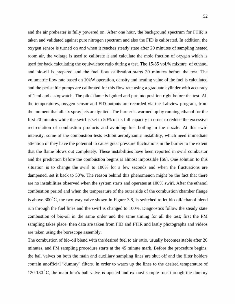
52
and the air preheater is fully powered on. After one hour, the background spectrum for FTIR is
taken and validated against pure nitrogen spectrum and also the FID is calibrated. In addition, the
oxygen sensor is turned on and when it reaches steady state after 20 minutes of sampling heated
room air, the voltage is used to calibrate it and calculate the mole fraction of oxygen which is
used for back calculating the equivalence ratio during a test. The 15/85 vol.% mixture of ethanol
and bio-oil is prepared and the fuel flow calibration starts 30 minutes before the test. The
volumetric flow rate based on 10kW operation, density and heating value of the fuel is calculated
and the peristaltic pumps are calibrated for this flow rate using a graduate cylinder with accuracy
of 1 ml and a stopwatch. The pilot flame is ignited and put into position right before the test. All
the temperatures, oxygen sensor and FID outputs are recorded via the Labview program, from
the moment that all six spray jets are ignited. The burner is warmed up by running ethanol for the
first 20 minutes while the swirl is set to 50% of its full capacity in order to reduce the excessive
recirculation of combustion products and avoiding fuel boiling in the nozzle. At this swirl
intensity, some of the combustion tests exhibit aerodynamic instability, which need immediate
attention or they have the potential to cause great pressure fluctuations in the burner to the extent
that the flame blows out completely. These instabilities have been reported in swirl combustor
and the prediction before the combustion begins is almost impossible [66]. One solution to this
situation is to change the swirl to 100% for a few seconds and when the fluctuations are
dampened, set it back to 50%. The reason behind this phenomenon might be the fact that there
are no instabilities observed when the system starts and operates at 100% swirl. After the ethanol
combustion period and when the temperature of the outer side of the combustion chamber flange
is above 300 C, the two-way valve shown in Figure 3.8, is switched to let bio-oil/ethanol blend
run through the fuel lines and the swirl is changed to 100%. Diagnostics follow the steady state
combustion of bio-oil in the same order and the same timing for all the test; first the PM
sampling takes place, then data are taken from FID and FTIR and lastly photographs and videos
are taken using the borescope assembly.
The combustion of bio-oil blend with the desired fuel to air ratio, usually becomes stable after 20
minutes, and PM sampling procedure starts at the 45 minute mark. Before the procedure begins,
the ball valves on both the main and auxiliary sampling lines are shut off and the filter holders
contain unofficial “dummy” filters. In order to warm up the lines to the desired temperature of
120-130 C, the main line’s ball valve is opened and exhaust sample runs through the dummy

53
filter. The sampling line is switched to the auxiliary line after 3-5 minutes before significant PM
accumulation and water condensation on the filter cause huge pressure drop. At this time, a
second dummy filter is placed in the filter holder of the main line. The second dummy filter
allows the line to reach the temperature that no significant water condensation occurs. Now that
the line is hot enough, the official filter replaces the second dummy. When the second dummy
filter is exposed to exhaust, the operator has to find the flow rate that makes the static pressure
difference between the sampling probe and the exhaust stream, shown on the manometer equal to
zero. This flow rate satisfies the isokinetic sampling condition and is an approximate of the
theoretical isokinetic flow rate of 10.4 % of the total exhaust flow rate (Appendix A). This
condition has to always be satisfied during sampling while the oxygen sensor shows the correct
equivalence ratio. The two official filters are consecutively positioned in the filter holder to take
samples of PM loading and are placed into their Petri dishes and capped immediately after
removal. During the official sampling, some parameters are recorded manually or automatically
by the data acquisition system and are later used for calculation of emissions. These parameters
include start/stop time of sampling on each filter, average dry gas temperature, sampling line
rotameter value, the exhaust oxygen concentration and condenser output pressure after each 1
minute mark.
When the PM sampling is done, the combustion air flow rate is adjusted and 5 minutes is
allocated for the system to reach steady state again. After this time, during a 5 minute period
before taking FTIR spectrum, the average amount of UHC is reported, and if a minor blow out
occurs during this time, data gets filtered such that the values that are at saturation point of FID
get discarded. The FTIR sampling begins at the hour mark and 5 spectrums are taken till 65-70
minutes. The pressure and temperature of the FTIR gas cell remains constant during the sample
for each test. The last instrument used for diagnostics is the borescope. Before opening the fitting
to place the borescope in, the pressure in the combustion chamber is recorded in order to bring
the system back at this pressure after insertion of the borescope to match the flame dynamics.
The tip of the tube is inserted such that cooling air is guided into the combustion chamber, and
meanwhile the stack fan and cooling air are ramped up slowly to avoid changing the chamber
pressure. The tube is then fully inserted to take photos and videos and taken out after each photo.
When all the data collection is completed, nozzle and fuel lines are cleaned by switching the fuel
back to ethanol. Since the system is already at a very high temperature, the air preheater is turned

54
off, the swirl is set back to 50 % and the nozzle cooling water is set to maximum in order to
avoid fuel boiling inside the nozzle. The system is shut down when the UHC reading reaches
below 20ppm which is usually after 20 minutes of running ethanol.
After letting the system to cool down, the deposits are scrubbed down from the nozzle tip and the
combustion chamber. Fuel lines and nozzle holes are fully cleaned from any bio-oil
contamination by running acetone through them. The PM sampling system is cleaned after each
test by shooting compressed air backwards through the sampling lines. All the water traps are
also emptied after each test.

55
4. Results and Discussion
4.1 Experimental Test Plan
To study the effect of natural and accelerated aging on the combustion performance and
emissions of bio-oil, a total of 14 official tests were carried out over a 10 months period. There
are two separate batches used for this project, both of which provided by the same manufacturer
and through the same production process. However, they possessed slightly different properties
and characteristic. The first batch was divided into two portions, one being aged naturally and
the other being aged in an accelerated fashion. Because of the limit in supply, the number of tests
for each method of aging was limited to 3 plus a base point at time zero. This batch served two
purposes: showing the effect of aging and validating the accelerated aging correlation. However,
in order to produce more data points and observe over an extended time period the effect of
aging, a second batch was ordered. Due to the time constraints of this project, the bio-oil from
this batch only underwent accelerated aging. A total of 7 experiments with different aging times
were performed with this second batch.
Small burners usually experience some problems with stability of the combustion. In order to
minimize this issue, all bio-oil batches were mixed with 15 % ethanol on a volumetric basis. The
burner parameters were optimized for bio-oil blend combustion in a previous study [46]. This
condition is called the “base” operating point which is presented in Table 4.1. The ranges that are
reported for equivalence ratio, air preheat temperature and primary combustion air flow rate are
due to the difference of basic properties in the two batches and also the limit in control accuracy
of the system. However, the fluctuations in these parameters are minute among all tests. In most
combustion applications, especially for heat and power generation, the power input is fixed.
Therefore, in all the tests, the fuel flow rate is adjusted to provide a power input of 10 kW based
on the heating value of the fuel. These changes in the flow rate of the bio-oil blend causes a
change in the air to fuel flow rate ratio in the nozzle which translates into variation in SMD. In
order to keep the SMD constant, the atomizing air flow rate needs to be modified for each
experiment. However, experience with pure ethanol as well as literature suggest that the
combustor flow field and mixing, flame stability and recirculation configuration is extremely

56
sensitive to the atomizing air [46]. Therefore, it was decided that a fixed atomizing air would be
used for all tests, in order to avoid any significant variation in flow characteristics between tests.
Table 4.1 – Base point Operating Condition
Swirl number 5.41
Power input from the blend 10 kW
Pilot power input 0.5 kW
Primary air preheater power 1.5 kW
Primary air temperature at the swirl box
inlet
320-337°C
Primary air flow rate 241-255 SLPM
Equivalence ratio 0.6-0.63
Atomizing air flow rate 23.2 SLPM
4.2 Experimental Results Summary
The fuel properties, calculated SMDs and emissions of the combustion tests under the base point
are presented in Table 4.2 and Table 4.3. The two different sections in the table are dedicated to
each batch and the labels show the number of months that the aging occurred and whether it was
natural (N) or accelerated (A). For example, 2A6 is the label used for the bio-oil from the second
batch that has underwent accelerated aging equivalent to 6 months of storage. The reason that
NOx is presented in a separate table here is that the main mechanism responsible for emissions
shown in Table 4.2 is incomplete combustion of bio-oil, while the mechanism behind NOx
formation is not related to incomplete combustion of the fuel [45]. This mechanism is described
in a separate section of this chapter.

57
Table 4.2 – Basic Fuel Properties and Emissions of Aged Pure Bio-oil
Batch
Label
Viscosity
(cSt)
Solids
(%mass)
TGA
Residue1
SMD
(µm)
CO
(ppm)
UHC
(ppm)
CR
(mg/MJ)
1N0 40.14 0.034 18.4 69.9 850 96 8.6
1N3 44.06 0.035 18.9 71.4 855 106 19.4
1N6 45.21 0.039 21.8 72.5 1120 159 13.6
1A6 49.03 0.038 20.4 74.2 1055 151 15.2
1N9 61.23 0.044 25.1 74.9 1216 212 27.3
1A9 56.04 0.042 23.3 75.7 1167 193 24.6
1A24 100.32 0.057 46.3 84.3 900 178 46.9
2N0 51.18 1.9 17.1 75.2 486 68 9.6
2A6 71.4 2.2 20.3 77.3 453 90 17.2
2A9 93.5 2.5 21.9 79.1 514 114 22.4
2A12 129.6 2.6 22.6 82.3 521 133 25.7
2A18 171.6 2.8 25.7 85.8 573 160 37.8
2A24 193.4 3.4 33.5 89.7 654 234 56.8
1 This measurement is done on the 85/15 vol.% mixture of bio-oil and ethanol

58
Table 4.3 - NOx Emissions of the Aged Bio-oil
Batch Label Fuel Nitrogen (mass%) NOx (ppm)
1N0 0.12 125
1N3 0.12 92
1N6 0.12 112
1A6 0.12 157
1N9 0.12 93
1A9 0.12 121
1A24 0.12 140
2N0 0.27 169
2A6 0.27 139
2A9 0.27 158
2A12 0.27 153
2A18 0.27 149
2A24 0.27 144
4.3 Mechanism of Pollution Formation from Bio-oil Combustion
As described in section 2.6, there are four primary stages in droplet combustion of bio-oil. In the
first stage, volatile gases evaporate from the surface of the droplet and produce a blue flame in a
homogenous combustion. Some of the gaseous emissions are formed in this stage, if incomplete
combustion occurs. When the volatiles tend to decrease, the flame extinguishes and only a char
particle remains which mostly consists of non-evaporative HMW molecules and solids and ash
particles. This char particle continues to burn in a solid state combustion mode, however char
burning can be distinguished in lower burner section because of its low temperature. The
temperature may even be so low that CO and UHC produced during char burnout cannot be
oxidized. The ash and carbonaceous residue that are left after the residence time are considered

59
the PM emissions. Figure 4.1 demonstrates the emissions produced at each stage of bio-oil
combustion.
Figure 4.1 – Pollutant Formation Mechanisms of Bio-oil Combustion [22]
High energy volatile materials, like alcohols, evaporate quickly and burn rapidly such that
complete combustion can be achieved. This fact can be used to reduce the gaseous emission such
as CO and UHC, by increasing the volatile content of bio-oil. These emissions are also formed
during the heterogeneous combustion of the char particle. Therefore, avoiding the formation of
char particles by reducing the solids content and HMW fraction of bio-oil, leads to a reduction in
CO and UHC emissions. Ash is mostly present in the solids content, and acts as catalyst for char
gasification, hence aiding the formation of CO and UHC in the heterogeneous combustion.
The particulate matter emissions mainly consist of CR and ash. Moloodi et al. concluded that
despite the complicated chemical composition of bio-oil, CR emission can be predicted by the
solids content and TGA residue of the fuel. Equation 4.1 demonstrates this linear correlation
[22]. As mentioned in section 3.2.3, TGA residue is a measure of the char formation potential of
the fuel and consists of HMW molecules, ash and solids. However, since the mass fraction of
HMW molecules is much larger than that of solids and ash, TGA residue can be treated as a
variable independent of solids and ash content.

60
( (
)
) (
) (
)
Equation
4.1 [22]
In order to do this linear regression analysis, the assumption was made that both of the
independent variables, solids content and TGA residue, vary in a small range. This analysis
sheds light on the effectiveness of each parameter in CR formation. The coefficient for TGA
residue is an order of magnitude larger than that of solids content, which means for small
burners, reducing TGA residue can help a lot in terms of reduction in PM emissions. Another
importance of this analysis is that an estimate of the CR emissions can be predicted without
having to perform an actual combustion test and by only doing a TGA, which is a much easier
test.
4.4 Analysis on the First Batch: Natural vs. Accelerated Aging
4.4.1 Fuel Properties
The fuel specification sheet from the producer of first batch reported a water content of 26.5 wt%
based on ASTM E203 test method and an ash content of 0.24 wt% based on ASTM D482 test
method. The other properties that follow were outsourced to Alberta Innovates-Technology
Futures. The carbon, hydrogen, nitrogen and oxygen mass fraction of the fuel are 40.78, 7.67,
0.12 and 51.43%, respectively. The gross heat of combustion measured at 25 C was reported to
be 16.91 MJ/kg.
The atom balance of the fuel was assumed to remain constant with aging while the viscosity,
solids content and TGA residue were measured after each aging period. All the results presented
in this section except the TGA residue data are for pure bio-oil. Figure 4.2 and Figure 4.3
demonstrate the viscosity of the fuel calculated with the handheld viscometer and measured
according to ASTM D445 at 40 C, respectively over the aging period. The values in Figure 4.2
and Figure 4.3 are very different because the viscosity that is calculated from the handheld
viscometer uses a correlation that was initially meant for water. Therefore, these calculated
values are not accurate and are just used to check the trend of viscosity before each combustion
test. As discussed in section 2.4.2, the viscosity is expected to increase with time of storage,
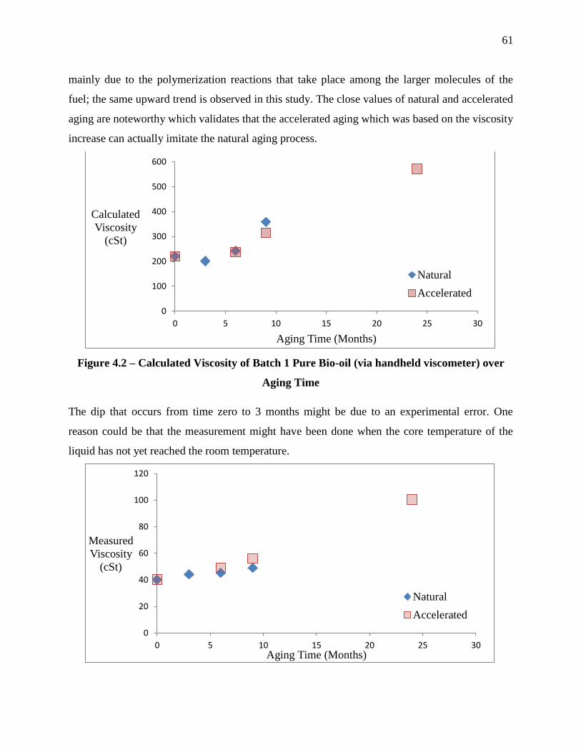
61
mainly due to the polymerization reactions that take place among the larger molecules of the
fuel; the same upward trend is observed in this study. The close values of natural and accelerated
aging are noteworthy which validates that the accelerated aging which was based on the viscosity
increase can actually imitate the natural aging process.
Figure 4.2 – Calculated Viscosity of Batch 1 Pure Bio-oil (via handheld viscometer) over
Aging Time
The dip that occurs from time zero to 3 months might be due to an experimental error. One
reason could be that the measurement might have been done when the core temperature of the
liquid has not yet reached the room temperature.
0
100
200
300
400
500
600
0 5 10 15 20 25 30
Calculated
Viscosity
(cSt)
Aging Time (Months)
Natural
Accelerated
0
20
40
60
80
100
120
0 5 10 15 20 25 30
Measured
Viscosity
(cSt)
Aging Time (Months)
Natural
Accelerated

62
Figure 4.3 – Measured Viscosity of Batch 1 Pure Bio-Oil (based on ASTM D445) over aging
time
The trend is evident here as well, however the increase in viscosity is very slow over the first 6
months and from this time forth, the rate of increase starts to climb.
The solids content of the bio-oil has shown an increase over time as well. This is mainly due to
the polymerization reactions discussed in section 2.3.2 and agglomeration of HMW molecules
into solid particles. The solids were measured through a non-conventional method (MeOH DCM
insoluble) where the fuel is dissolved in methanol and the fraction that is not soluble is the solids
content. Figure 4.4 demonstrates the increase in solids content for both naturally and accelerated
aged samples over the aging period.
Figure 4.4 – Solids Content of Batch 1 Pure Bio-oil vs. Aging Time
The TGA residue is described as a measure of the tendency of the fuel to evaporate in section
2.7.2 and the effect of aging on fuel’s volatility is explained in section 2.4.5. It is expected that
TGA residue increases over time mainly because of the polymerization reactions that take place
in the fuel over time and increase the HMW molecular fraction of the fuel. In addition, the gas
forming reactions mentioned in section 2.3.4 cause the volatiles to exit the liquid fuel and
accumulate on top of the bottle and escape as soon as the cap is opened. Figure 4.5 demonstrates
the effect of aging on the TGA residue of 85/15 volumetric bio-oil/ethanol blends.
0
0.01
0.02
0.03
0.04
0.05
0.06
0 5 10 15 20 25
Soli
ds
Conte
nt
(% m
ass)
Aging Time (Months)
Natural
Accelerated

63
Figure 4.5 – Effect of Aging on the first batch blends’TGAresidue
As can be seen in all these graphs, the effect of aging on physical properties start to kick in some
time after the first three months of aging, and for the two years of aging case, the increase is
substantial suggesting a somewhat exponential relationship between time of storage and the
increase in values of each physical property.
4.4.2 Gaseous Emissions
The main gaseous emissions that were considered in this aging study were CO & UHC that were
caused by incomplete combustion of the fuel spray. The other important gaseous emission is
NOx which is discussed in section 4.5. Figure 4.6 shows the effect of aging on CO emissions for
this batch. There is almost no change in the first 3 months corresponding to the small changes in
physical properties over this period, but the major increase occurs after this time through the 9
months data point. However, the value for the 2 year accelerated emission is not following the
trend and is actually lower that the 6 months value.
0
5
10
15
20
25
30
35
40
45
50
0 5 10 15 20 25
TG
A R
esid
ue
(% m
ass)
Aging Time (Months)
Natural
Accelerated

64
Figure 4.6 – CO emissions for Batch 1 Blends vs. Aging Time
Previous studies have shown that CO and UHC trends follow each other closely [46], [22].
Error! Reference source not found. confirms this observation, where a slight increase is
etected for the first 3 months and after that the jumps in values for 6 and 9 months are observed,
followed by the decline for the 24 months.
Figure 4.7 - UHC emissions for Batch 1 Blends vs. Aging Time
0
200
400
600
800
1000
1200
1400
0 5 10 15 20 25
CO
(p
pm
)
Aging Time (Months)
Accelerated
Natural
0
50
100
150
200
250
0 5 10 15 20 25
UH
C (
ppm
)
Aging Time (Months)
Natural
Accelerated
65
The behavior that is seen for 2 years of aging can be explained in terms of the PM emissions of
the fuel which is discussed in section 4.3.3. The fuel quality and the combustion performance is
so poor that the fuel droplets cannot be burned fully in the first stage of combustion and the
abundance of the char particles that are produced after this stage, don’t have adequate residence
time to burn the carbon fraction in a heterogeneous combustion. Therefore, as aging progresses
more of the fuel is not even burnt to produce any gaseous emissions and more of the fuel just
escapes in the form of particulate matter.
The close values of gaseous emissions of naturally and accelerated aged bio-oil suggests that the
accelerated aging method produces a very similar liquid to the one that is naturally aged.
Therefore, in order to save time for a study, natural aging can be substituted with the heating of
bio-oil at a higher temperature and the corresponding calculated time base on the correlation.
4.4.3 PM Emissions
Figure 4.8 shows the effect of aging on carbonaceous residue emissions of the bio-oil blends. It
is observed that the PM emissions go up as more time is allocated for storage. This is attributed
to the loss of volatiles during aging that makes the combustion of the fuel more difficult because
the high energy volatile material that help stabilize and enhance the combustion are decreasing in
volume over time. Also, the polymerization reactions increase the HMW molecules fraction of
the fuel which makes the droplets denser and thus heavier. These denser droplets are more
difficult to penetrate with the free radicals for complete combustion. For the purpose of this
study, because the energy throughput of the burner is fixed to 10 kW for all tests, the
carbonaceous residue emission of combustion of bio-oil blends is normalized by the energy of
the fuel that goes through the system and is presented in units of mg/MJ.

66
Figure 4.8 – CR Emissions of Batch 1 Blends over the Aging Period
The inconsistency of the 3 months data might be because of a small instability and partial blow-
out during the PM sampling period. There are many parameters involved in the combustion of
bio-oil blends in the confined geometry of the burner, some of which are not controllable with
the current setup. One example is the pressure build-up in the combustion chamber which
extinguishes the flame momentarily.
The very high value of CR for 24 months of aging can be explained with Equation 4.1. Both the
TGA residue and the solids content of the 2 years accelerated aged bio-oil are much higher
compared the data for earlier times. The TGA residue has jumped 150% compared to base point
and solids content has increased 81%. As mentioned before, the effect of TGA residue is an
order of magnitude higher than solids content and the substantial increase in CR emissions is not
surprising. Figure 4.9 compares the CR values obtained from experiments with the values
predicted by Equation 4.1. Although the values are not matching closely, the trend is captured
well by the equation. The main reason is that the linear regression was performed on a set of data
that was obtained from a different batch with different fuel properties.
0
10
20
30
40
50
0 5 10 15 20 25
CR
(mg/M
J)
Aging Time (Months)
Natural
Accelerated

67
Figure 4.9 – Comparison of Calculated and Measured CR for Batch 1 Blends
4.4.4 Flame Visualization
Photographs taken during each combustion test, using the borescope assembly are presented in
Figure 4.10. The combustion performance can be examined visually in these pictures. As the
time of aging increase, the flame quality becomes poorer and more glowing particles burning is
detected.
1N0 1N3 1N6
0
500
1000
1500
2000
2500
3000
3500
0 5 10 15 20 25 30
CR
(m
g/kg
fu
el)
Aging Time (Months)
Experiment Natural
Experiment Accelerated
Calculated Natural
Calculated Accelerated

68
1A6 1N9 1A9
1A24
Figure 4.10 – Borescopic Photos of batch 1 bio-oil blend combustion
4.5 Analysis on the Second Batch: Long Term Accelerated Aging
4.5.1 Fuel Properties
After confirming that the method of accelerated aging produces a similar liquid to natural aging
in terms of physical properties and combustion performance, and in order to fill in the gap
between 9 months and 24 months of aging, a second batch was ordered. Therefore batch 2 was
provided at a later time than batch 1 and although it was produced in the same pyrolysis plant as
the first batch, it had different physical characteristics. The manufacturer reported the water
content and ash content to be 23 wt% and 0.26 wt% respectively. However the solids content is
much higher than the previous batch at the value of 1.9 wt%. The Carbon, Hydrogen, Nitrogen

69
and Oxygen mass fractions are 43.45, 7.38, 0.27 and 48.90%. The gross of heat of combustion is
reported as 18.2 MJ/kg which is higher compared to the first batch; therefore a smaller fuel flow
rate is required for the operation of the system at 10 kW.
Figure 4.11 shows that the viscosity of the second batch bio-oil calculated with the time data
obtained from the handheld viscometer, increases with aging time. There is no data point
presented for 2 years of aging in this graph, because the liquid formed solid gel-like chunks that
would restrict the flow through the handheld viscometer orifice. The 1 year aging was first
produced and a full set of physical and emissions measurement was done on it, however the
results did not seem to be correct. All other tests were done after that to make sure that this data
point is the one that needs to be repeated. When confirmed, a new bottle of bio-oil was taken out
of the fridge and the complete aging and testing process was repeated. The discrepancy of the
first point must have been due to the aging process and some malfunctioning of the oven over
night. Another point that can be seen in this graph is that the rate of viscosity increases in the
first 9 months of aging and reduces after that.
Figure 4.11 - Calculated Viscosity of Batch 2 (via handheld viscometer) over Aging Time
The measured viscosity via ASTM D445 test method of the fuel after each aging period is
presented in Figure 4.12. The viscosity measurement after 24 month of aging was possible with
this method. The same trend is seen here as well, the slope of the line segments between each
consecutive data points decrease after the 6 months. This means that as time passes by, the
viscosity increases more slowly. The same is trend is seen in Figure 2.8 [37]. The same issue
0
100
200
300
400
500
600
700
0 5 10 15 20
Cal
cula
ted V
isco
sity
(cS
t)
Aging Time (Months)
Accelerated

70
discussed for the 1 year of aging shows up here as well. An inconsistent dip was suspicious and
proved to be an error in the aging process of the fuel.
Figure 4.12 - Measured Viscosity of Batch 2 (based on ASTM D445) over Aging Time
The solids content of this new batch was almost 2 orders of magnitude larger than the first batch.
The changes made to the amount of solids over the aging period are demonstrated in Figure 4.13.
The abundance of solids accelerates the polymerization reactions and enhances the
agglomeration of the particle to an extent that visual inspection of the 24 months aged bio-oil
concluded the presence of gel-like solid chunks in the liquid. The solid content was also visibly
flowing in the fuel lines during the tests. The solids content of batch 2 bio-oil increases steadily
with the aging time and the trend can almost be approximated by a linear function.
0
50
100
150
200
0 5 10 15 20 25
Mea
sure
d V
isco
sity
(cS
t)
Aging Time (Months)
Accelerated

71
Figure 4.13 - Solids Content of Batch 1 vs. Aging Time
TGA residue of this batch shows an upward trend over time as well; however the value at each
point of time is less compared to batch 1. The rate of increase in TGA residue shows a different
behavior than viscosity over the course of aging time for this fuel. The increase starts slower and
picks up after a year of aging, with the biggest jump being for 18 months to 24 months. These
results are presented in Figure 4.14.
1
1.5
2
2.5
3
3.5
4
0 5 10 15 20 25 30
Soli
ds
Conte
nt
(%m
ass)
Aging Time (Months)
Accelerated
10
15
20
25
30
35
0 5 10 15 20 25
TG
A R
esid
ue
(%m
ass)
Aging Time (Months)
Accelerated

72
Figure 4.14 - Effect of Aging on the second batch blends’TGAresidue
The addition of ethanol before conducting the TG analysis broke apart the gel-like solids that
were present after 24 months of aging and there was no sign of them after pouring the blend into
another container. However, as the very high TGA residue value suggests, the polymerization of
the HMW weight molecules have made the evaporation of them much more difficult.
4.5.2 Gaseous Emissions
Figure 4.15 presents the CO emissions of the combustion of bio-oil blend as the aging time is
varied. As the fuel quality and evaporation decreases over time, complete combustion of the
volatiles in the first stage of combustion and burning of the char in the third stage become more
challenging. This results in increasing CO emissions over the aging period. The discrepancy
between the base and 6 months points can be discussed. One possibility is that the value of CO
for the base point is overestimated and the other option is that the 6 month might be
underestimated. If the fuel properties are taken into consideration, all three show an increase over
this period. However, the slope of the line from base to 6 months is less than that of the line from
6 to 9 months of aging. Based on previous studies performed on the effect of fuel properties on
combustion, we can conclude that the base point data is an off point and has to be slightly lower
than the 6 months data point [22]. The reason for this could be explained in terms of partial
blow-outs that occur in the burner from time to time during the test. When a blow-out occurs fuel
is sprayed on the walls as well without undergoing combustion. This deposited fuel starts to
gasify in the very hot environment of the combustion chamber and emits carbon monoxide as
one the gasification products. Another reason could be that the only possible way for having an
underestimated CO value, considering the sampling method and 5 consecutive spectrums is that
the sampling lines are not hot enough such that condensation occurs in the FTIR. However, this
was not the case for the 6 months experiment, and all the temperatures looked normal during the
FTIR sampling period.

73
Figure 4.15 - CO emissions for Batch 2 vs. Aging Time
Also, if we take a look at the effect of aging on the UHC emissions for the second bio-oil batch,
which is demonstrated in Figure 4.16, and keeping in mind that UHC and CO emissions usually
follow each other, we can confirm that the base data point is overestimated in these results. The
increasing trend can be seen here as well, with the rate of emission increase becoming larger
after 12 months of aging.
Figure 4.16 - CO emissions for Batch 2 vs. Aging Time
4.5.3 PM Emissions
The solids content and TGA residue of this fuel suggest that an increasing CR emissions trend
should be expected based on the prediction of Equation 4.1. Figure 4.17 demonstrates that this
400
450
500
550
600
650
0 5 10 15 20 25
CO
(p
pm
)
Aging Time (months)
Accelerated
0
50
100
150
200
250
0 5 10 15 20 25
UHC
(ppm)
Aging Time (Months)
Accelerated

74
expectation is reasonable and in fact the CR emission for the second batch shows an increase
with the aging time. Also the trend in rate of increase in CR follows the same trend as the rate of
increase in TGA residue, where the slope between the successive points becomes larger after the
first year of aging. When compared to the first batch, the TGA residue for both of them is in the
same range but the solids content of batch 2 is almost two orders of magnitude larger than that of
batch 1. This is the reason fo the higher values of CR emission of batch 2. However, the effect of
solids on the CR emission is much less than the TGA residue and this explains why the increase
in CR values between the two batches is not as high as the jump in the solids content.
The main driving force for repeating the 12 months data point was the huge dip in value from the
previous experiment which was the 6 months of aging. After that, when the 9 months experiment
was conducted and showed a higher value than both 6 months and 12 months, it was confirmed
that not only the aging process of the one year point had some issues because of discrepancies in
physical properties values, but also the PM sampling of this point was faulty because it provided
the same value as the base point in spite of the increase in TGA residue.
Figure 4.17 - CR Emissions of Batch 2 Blends over the Aging Period
Figure 4.18 show a comparison between the calculated CR using Equation 4.1 and the measured
CR during experiments. Although the values do not match, the same trend is seen in both sets of
data. The difference in values between them is mainly because of linear regression coefficients
which were optimized for another batch of fuel with different properties.
0
10
20
30
40
50
60
70
0 5 10 15 20 25
CR
(mg/M
J)
Time (months)
Accelerated

75
Figure 4.18 - Comparison of Calculated and Measured CR for Batch 2 Blends
4.5.4 Flame Visualization
The qualitative comparison between the flames is carried out visually by taking photographs
during the combustion test and inspection the changes in flame dynamics that contribute to the
emissions. Figure 4.19 presents these pictures in the chronological order. As the time of aging is
increased, the combustion quality of the flame is lowered and as can be seen in the pictures,
more PM char burnout occurs which is identified as the glowing particles.
0
500
1000
1500
2000
2500
3000
3500
0 5 10 15 20 25 30
CR
(m
g/kg
fu
el)
Aging Time (Months)
Experiment Accelerated
Calculated Accelerated

76
2A0 2A6 2A9
2A12 2A18 2A24
Figure 4.19 – Borescopic Photos of batch 2 bio-oil blends combustion
4.6 NOx Emissions
NOx is the sum of nitrogen oxide and nitrogen dioxide in the exhaust. There are three major
mechanisms of NOx formation that are dependent on operating conditions and fuel chemistry:
prompt, thermal and fuel NOx [45]. Prompt NOx formation is described as the scission of the
nitrogen molecules in air via their reactions with free radicals of hydrocarbons that are mostly
present in flame fronts. This mechanism usually has a minor contribution to the overall NOx. The
thermal NOx formation is very temperature sensitive and occurs at high temperatures. It is mainly
due to the reactions of air nitrogen with oxygen and OH radicals. Fuel NOx forms from fuel
bound nitrogen during combustion and is mainly controlled by the stoichiometry. The formation
of NOx is weakly dependent on temperature in this mechanism. The literature that has studied the
NOx formation in bio-oil combustion has shown that the dominant mechanism of NOx formation
is fuel NOx [46], [67]. Figure 4.20 shows the effect of aging on NOx for the first batch. A slight
decreasing trend is seen for both cases.

77
Figure 4.20 – NOx emissions of Batch 1 Blends over Aging Period
This trend is more obvious in the NOx emissions of the second batch. Figure 4.21 presents the
NOx data for this batch as the time of aging is increased. The best fit line shown on the graph has
a slight negative slope, which can be described in terms of CO and UHC emissions. It has been
shown in previous section that as the aging time is increased, these emissions go up because of
lower burning quality and heavier incomplete combustion. These phenomena cause the flame
temperature and as a result the burner temperature to decrease. As described earlier, thermal NOx
is formed at high temperatures and as the temperature is lowered, this value decrease too.
However, the dominance of thermal NOx formations is less than the fuel NOx formation and
therefore, the decrease in value is much less than the total value. In addition, another reason for
this decrease could be the increase in PM emission. As more PM is produced, more of the fuel
escapes without fully oxidizing. Therefore, more fuel nitrogen which is still bound to the PM
does not burn in order to form any NOx.
0
30
60
90
120
150
0 3 6 9 12 15 18 21 24
NO
x (
ppm
)
Aging Time (months)
Natural
Accelerated

78
Figure 4.21 - NOx emissions of batch 2 over Aging Period
4.7 Acetaldehyde, Formaldehyde and Methane Emissions
The emissions of acetaldehyde, formaldehyde and methane for most of the aged bio-oil blends
were below detection (BD) limits of the FTIR. These emissions are mainly the product of poor
and unstable combustion conditions. Therefore, they are detected when the UHC values are high.
Table 4.4 lists the values for these emissions.
Table 4.4 – Emissions for Selected Blends
Batch
Label
CH4
(ppm)
CH2O
(ppm)
C2H4O
(ppm)
1N9 BD 16 BD
1A9 BD 13 BD
1A24 35 50 95
2A12 BD 22 28
2A18 17 28 46
2A24 39 46 82
y = -0.6876x + 161.67
0
30
60
90
120
150
180
0 3 6 9 12 15 18 21 24
NO
x (
ppm
)
Aging Time (Months)
Accelerated

79
5. Conclusions and Recommendations
5.1 Conclusions
The aging process is very sensitive to temperature and the kinetics of the chemistry is accelerated
as the liquid temperature increases.
The results show that the fuel quality of bio-oil becomes poorer as it is stored for longer periods
of time. Viscosity, which is a crucial factor in atomization quality, increases with time. Also,
solids content and TGA residue of the fuel, which is a measure of fuel polymerization, show an
increase with aging.
The amount of particulate carbonaceous residue was calculated. There is an upward trend in CR
emission with aging time which follows the shape of the graph of TGA residue. In addition, the
batch with much higher solids content produced more CR emission while the TGA residues were
close but still the dominating factor. The trend was predicted by an equation relating CR
emissions with solids content and TGA residue. This suggests that aging increases the solids
content and polymerization (TGA residue) of the fuel. As a result, there is more char formation
during burnout which causes more CR emissions.
The major gaseous emissions considered in this study are CO and UHC. They follow each
other’s increasing trend and reach a higher rate of increase as more time passes. They also follow
the increasing trend of CR emissions.
The results show a slight decrease in NOx emission over the aging period. This is due to both
thermal NOx formation mechanism and the amount of fuel nitrogen trapped in the PM emission.
The higher CO and UHC emissions prove a more incomplete combustion with lower temperature
inside the burner. Thermal NOx is decreased when the temperature is lowered. Moreover, NOx
formation in bio-oil combustion is dominated by fuel bound nitrogen and as more PM emissions
is formed, less fuel nitrogen is available for combustion and thus the decreasing trend is
observed.
To summarize, aging has a detrimental effect on the fuel quality of bio-oil which results in
higher combustion emissions. Therefore, a few solutions can be sought to minimize this effect.
The bio-oil should be kept in a cool place above the freezing point in order to delay the aging
process. Bio-oil should also be stored in sealed containers in order to avoid any air exposure.

80
Leaving the fuel in an open container, would let the high energy volatiles escape and also
accelerate the polymerization reactions. Another effective approach is to add a solvent such as
ethanol, as soon as the bio-oil is produced. The solvent retards the aging reactions significantly
and also improves the quality of the fuel for combustion. However, the best way to handle a
problem is to eliminate it. The best option is to use bio-oil as a renewable source to produce heat
and power, near the production plant and with the minimum storage time required.
5.2 Recommendations
1. In order to improve the combustion efficiency and reduce THC and CO emissions, a
refractory lining could be added to the burner system. The insulation would mitigate the
heat losses through walls and bring their temperatures higher such that wall quenching
effects are minimized.
2. If the bio-oil is burned under rich conditions, fuel bound nitrogen is more favored to
convert to N2 [45]. Therefore, if this could happen in the first stage of staged combustion,
NOx reduction could be achieved. More air would be provided for the second stage to
reach complete combustion.
3. The axial momentum of the atomizing air jets is so high that it penetrates through the
central recirculation zone and negatively impacts the stability of combustion. Therefore,
designing a nozzle that can atomize bio-oil at very low flow rates of atomizing air would
be beneficial. The best option for such a design would output an axisymmetric hollow-
cone spray pattern.
4. In the present setup, FID and FTIR sampling cannot be performed simultaneously. The
connections used for the heated line can be replaced by a T-section to enable these two
systems to draw from the sampling line at the same time.
5.3 Future Works
1. Atomization quality has a great impact on combustion performance and emissions.
Droplet size and velocity measurements would provide insight into interpretation of the
results.

81
2. Another parameter that has a significant effect on emission trends is the complicated flow
pattern in the combustion chamber. Details of velocity vector field in the burner could be
measured which would shed light on the flame dynamics and central recirculation zone.
3. In order to reduce the consumption of fossil fuels such as diesel and No. 4 fuel oil and
replace it with renewable energy source such as bio-oil, the first step could be to use a
blend of them in small scale combined heat and power units. The blending would be
achieved by mechanical or chemical emulsification of the two fuels. Blends with
different ratios of diesel and bio-oil could be burned in the burner and emissions would
be analyzed to choose the best mixture.
4. The effect of different light intensity exposure to bio-oil during storage time can be
investigated by comparing the emission trends of combustion in this spray burner.
5. Heating rate of the accelerated aging method could be varied and the results of the
combustion tests could be examined to analyze the impact of different heating rates.

82
Bibliography
[1] A. F. Ghoniem, "Needs, resources and climate change: Clean and efficient conversion
technologies," Progress in Energy and Combustion Science, vol. 37, pp. 15-51, 2011.
[2] A. V. Bridgwater, "Renewable fuels and chamicals by thermal processing of biomass,"
Chemical Engineering Journal, vol. 91, pp. 87-102, 2003.
[3] J. Koppejan, "Challenges in biomass and cofiring: the work of IEA Bioenergy Task 32," in
IEA Bioenergy Conference, Vancouver, British Columbia, 2009.
[4] L. Petrus and M. A. Noordermeer, "Biomass to Biofuels, a chemical perspective," Green
Chemistry, vol. 8, no. 10, pp. 861-867, 2006.
[5] A. V. Bridgwater, "Biomass Pyrolysis," Report IEA Bioenergy, 2007.
[6] S. P. Krumdieck and J. W. Daily, "Evaluating the Feasibility of Pyrolysis Oil for Spray
Combustion Applicatons," Combustion Science and Technology, vol. 134, no. 1, pp. 351-
365, 1998.
[7] T. Tzanetakis, N. Farra, S. Moloodi, W. Lamont, A. McGrath and M. J. Thomson, "Spray
Combustion Characteristics and Gaseous Emissions of a Wood Derived Fast Pyrolysis
Liquid-Ethanol Blend in a Pilot Stabilized Swirl Burner," Energy & Fuels, vol. 24, pp.
5331-5348, 2010.
[8] T. Tzanetakis, S. Moloodi, N. Farra, B. Nguyen and M. J. Thomson, "Spray Combustion
and Particulate Matter Emissions of a Wood Derived Fast Pyrolysis Liquid-Ethanol Blend
in a Pilot Stabilized Swirl Burner," Energy & Fuels, vol. 25, pp. 1405-1422, 2011.
[9] D. Meier and O. Faix, "State of the Art of Applied Pyrolysis of Lignocellulosic Materials,"
Bioresource Technology, vol. 68, pp. 71-77, 1999.
[10] A. V. Bridgwater and G. V. C. Peacocke, "Fast Pyrolysis Processes for Biomass,"
Renewable and Sustainable Energy Reviews, vol. 4, no. 1, pp. 1-73, 2000.
[11] D. Mohan, C. U. Pittman and P. H. Steele, "Pyrolysis of Wood/Biomass for Bio-oil: a
Critical Review," Energy & Fuels, vol. 20, no. 3, pp. 848-889, 2006.

83
[12] C. Xu Linghong Zhang and P. Champagne, "Overview of Recent Advances in Thermo-
Chemical Conversion of Biomass," Energy Conversion and Management, vol. 51, pp. 969-
982, 2010.
[13] L. Qiang, L. Wen-Zhi and Z. Xi-Feng, "Overview of Fuel Properties of Biomass Fast
Pyrolysis Oils," Energy Conversion and Management, vol. 50, pp. 1376-1383, 2009.
[14] T. Ba, A. Chaala, M. Garcia-Perez, D. Rodrigue and C. Roy, "Colloidal properties of bio-
oils obtained by vaccum pyrolysis of softwood bark. Characteriziation of water-soluble and
water-insoluble fractions," Energy & Fuels, vol. 18, pp. 704-712, 2004.
[15] A. Oasmaa, E. Kuoppala and Y. Solantausta, "Fast pyrolysis of forestry residue. 2.
physiochemical composition of product liquid," Energy & Fuels, vol. 17, no. 2, pp. 433-
443, 2003.
[16] A. Oasmaa and S. Czernik, "Fuel oil quality of biomass pyrolysis oils - state of the art for
end users," Energy & Fuels, vol. 13, no. 4, pp. 914-921, 1999.
[17] S. Czernik and A. V. Brdigwater, "Overview of applications of biomass fast pyrolysis oil,"
Energy & Fuels, vol. 18, no. 2, pp. 590-598, 2004.
[18] C. R. Shaddix and D. R. Hardesty, "Combustion properties of biomass flash pyrolysis oils:
Final project report," Tech. Rep. SAND998238, Sandina National Laboratories, 1999.
[19] M. E. Boucher, A. Chaala and C. Roy, "Bio-oils obtained by vaccum pyrolysis of softwood
bark as liquid fuel for gas turbines. part i: properties of bio-oil and its blends with methanol
and a pyrolytic aqueous phase," Biomass and Bioenergy, vol. 19, pp. 337-350, 2000.
[20] A. Oasmaa, E. Leppamaki, P. Koponen, J. Levander and E. Tapola, Physical
Characterization of biomass-base pyrolysis liquids: application of standard fuel oil
analyses, VTT Energy Publication 306, 1997.
[21] D. C. Elliott, "Warer, alkali and char in flash pyrolysis oils," Biomass and Bioenergy, vol. 7,
pp. 179-185, 1994.
[22] S. Moloodi, "Experimental Investigation of the effects of Fuel Properties on Combustion
Performance and Emissions of Biomass Fast Pyrolysis Liquid-Ethanol Blends in a Swirl
Burner," Mechanical and Industrial Engineering, University of Toronto, MASc Thesis 2011.
[23] S. Abglevor and S. Besler, "Inorganic Compounds in Biomass Feedstock. 1. Effect on the

84
Quality of Fast Pyrolysis Oils," Energy & Fuels, vol. 10, pp. 293-298, 1996.
[24] C. Branca and C. Di Blasi, "Devolatilization and Heterogeneous Combustion of Wood Fast
Pyrolysis Oils," Industrial & Engineering Chemistry Research, vol. 44, pp. 799-810, 2005.
[25] A. Chaala, T. Ba, M. Garcia-Perez and C. Roy, "Colloidal Properties of Bio-oils Obtained
byVacuum Pyrolysis of Softwood Bark: Aging and Thermal Stability," Energy & Fuels,
vol. 18, pp. 1535-1542, 2004.
[26] P. Bhattaharya, E. Hassan, P. Steele, J. Cooper and L. Ingram, "Effect of Acid Catalysts and
Accelerated Aging on the Reaction of Methanol with Hydroxy-Acetaldehyde in Bio-Oil,"
BioResources, vol. 5, no. 2, pp. 908-919, 2010.
[27] S. Czernik, D. K. Johnson and S. Black, "Stability of Wood Fast Pyrolysis Oil," Biomass
and Bioenergy, vol. 7, pp. 187-192, 1994.
[28] A. Oasmaa, E. Kuoppala and Y. Solantausta, "Fast Pyrloysis of Forestry Residue. 1. Effect
of Extractves on Phase Seperation of Pyrolysis Liquids," Energy & Fuels, vol. 17, no. 1, pp.
1-12, 2003.
[29] R. M. Simons, "Esterification," in Encyclopedia of Chemical Processing and Design, New
York, Marcel Dekker, 1983, p. 381.
[30] D. A. G. Radlein, J. K. Piskorz and P. A. Majerski, "Method of Upgrading Biomass
Pyrolysis Liquids for Use as Fuels and as a Source of Chemicals by Reaction with
Alcohols". European Patent Application Patent EP19950309400, 1 9 1999.
[31] J. F. Walker, Formaldehyde, New York: Reinhold Publishing Corp., 1944, p. 397.
[32] J. P. Diebold and S. Czernik, "Additives To Lower and Stabilize the Viscosity of," Energy
& Fuels, vol. 11, pp. 1081-1091, 1997.
[33] J. P. Diebold, "A Review of the Chemical and Physical Mechanisms of the Storage Stability
of Fast Pyrolysis Bio-Oils," National Renewable Energy Laboratory, Golden, Colorado,
2000.
[34] F. A. Carey, Organic Chemistry, 3rd ed, NY: McGraw-Hill, 1996.
[35] W. Fiddler, W. E. Parker, A. E. Wasserman and R. C. Doerr, "Thermal Decomposition of
Ferulic Acid," Agricultural & Food Chemistry, vol. 15, no. 5, p. 757–761, 1967.
[36] G. Peacocke, P. Russel, J. Jenkins and A. Bridgwater, "Physical Properties of Flash

85
Pyrolysis Liquids," Biomass and Bioenergy, vol. 7, no. 1, pp. 169-177, 1994.
[37] A. Oasmaa and E. Kuoppala, "Fast Pyrolysis of Forestry Residue. 3. Storage Stability of
Liquid Fuel," Energy & Fuels, vol. 17, pp. 1075-1084, 2003.
[38] M. Garcia-Perez, A. Chaala, H. Pakdel, D. Kretschmer, D. Rodrigue and C. Roy,
"Multiphase Structure of Bio-Oils," Energy & Fuels, vol. 20, pp. 364-375, 2006.
[39] F. Yu, S. Deng, P. Chen, Y. Liu, Y. Wan, A. Olson, D. Kittelson and R. Ruan, "Physical
and Chemical Properties of Bio-Oils From Microwave Pyrolysis of Corn Stover," APPLIED
BIOCHEMISTRY AND BIOTECNOLOGY, vol. 7, pp. 957-970, 2007.
[40] M. E. Boucher, A. Chaala, H. Pakdel and C. Roy, "Bio-Oils Obtained by Vacuum Pyrolysis
of Softwood Bark as a Liquid Fuel for Gas Turbines. Part II: Stability and Ageing of Bio-oil
and its Blends with Methanol and a Pyrolytic Aqueous Phase," Biomass & Bioenegy, vol.
19, pp. 351-361, 2000.
[41] M. Polk and M. Phingbodhippakkiya, "Development of Methods for the Stabilization of
Pyrolytic Oils," Municipal Environmental Research Laboratory, U.S. Environmental
Protection Agency, Cincinnati, OH, 1981.
[42] I. Tiplady, G. Peacocke and A. Bridgwater, "Physical Properties of Fast Pyrolysis Liquids
from the Union Fenosa Pilot Plant," in Bio-Oil Production and Utilization, Newbury, CPL
Press, 1996, pp. 164-174.
[43] M. Wornat, B. Porter and N. Yang, "Single Droplet Combustion of Biomass Pyrolysis Oils,"
Energy & Fuels, vol. 8, no. 5, pp. 1131-1142, 1994.
[44] M. Garcìa - Pèrez, P. Lappas, P. Hughes, L. Dell, A. Chaala, D. Kretschmer and C. Roy,
"Evaporation and combution characteristics of biomass vacuum pyrolysis oils," IFRF
Combustion Journal, vol. Article 200601, pp. 1-28, May 2006.
[45] S. R. Turns, An introduction to combustion: concept and application, 2nd ed., McGraw-Hill
Higher Education, 2000.
[46] T. Tzanetakis, "Spray Combustion Characteristics and Emissions of a Wood Derived Fast
Pyrolysis Liquid-Ethanol Blend in a Pilot Stablizied Swirl Burner," Mechanical and
Industrial Engineering, University of Toronto, PhD Thesis 2011.
[47] A. Shihadeh and S. Hochgreb, "Impact of biomass pyrolysis oil process conditions on

86
ignition delay in compression ignition engines," Energy & Fuels, vol. 16, pp. 552-561,
2002.
[48] C. R. Shaddix and P. J. Tennison, "Effects of Char Content and Simple Additives on
Biomass Pyrolysis Oil Droplet Combustion," in 27th Symposium (International) on
Combustion, 1998.
[49] M. J. Veraa and A. T. Bell, "Effect of alkali metal catalysts on gasification of coal char,"
Fuel, vol. 57, 1978.
[50] A. Gupta, D. Lilley and N. Syred, Swirl Flows, Gordon and Breach Publishers, 1984.
[51] J. Beer and N. Chigier, Combustion Aerodynamcis, Applied Science Publishers, 1972.
[52] Catalog No. JPL99C, JPL Series Air Atomizing Nozzles, Mississauga, ON, Canada: BEX
Engineering Ltd., 2008.
[53] E. Sher, T. Bar-Kohany and A. Rashkovan, "Flash-Boiling Atomization," Progress in
Energy & Combustion Science, vol. 34, pp. 417-439, 2008.
[54] M. Radovanovic, R. Vanderbosch, W. Prins and W. Van Swaaji, "Some remarks on the
viscosity measurement of pyrolysis liquids," Biomass and Bioenergy, vol. 18, pp. 209-222,
2000.
[55] K. Schofield, "The enigmatic mechanism of flame ionization detector: Its overlooked
implications for fossil fuel combustion modeling," Progress in Energy and Combustion
Science, vol. 34, pp. 330-350, 2008.
[56] P. Griffiths and J. De Haseth, Fourier Transform Infrared Spectrometry, 2nd ed., John Wiley
and Sons, 2007.
[57] N. Farra, "Efficiency and Emissions Study of a Residential Micro-Cogeneration System
Based on a Stirling Engine and Fuelled by Diesel and Ethanol," MASc. Thesis, University
of Toronto, 2010.
[58] R. Dennis, W. Samples, D. Anderson and L. Silverman, "Isokinetic sampling probes,"
Industrial and Engineering Chemistry, vol. 49, no. 2, pp. 294-302, 1957.
[59] M. D. Durham and D. A. Lundgren, "Evaluation of aerosol aspiration efficiency as a
function of stokes number, velocity ratio and nozzle angle," Journal of Aerosol Science, vol.
11, pp. 179-188, 1980.

87
[60] S. Badzioch, "Collection of gas-borne dust particles by means of an aspirated sampling
nozzle," British Journal of Applied Physics, vol. 10, no. 1, pp. 26-32, 1959.
[61] "EPA Method 5- determination of particulate matter emissions from stationary sources".
[62] H. Altgeld, W. Jones and J. Wilhelmi, "Velocity measurements in a confined swirl driven
recirculating flow," Experiments in Fluids, vol. 1, pp. 73-78, 1983.
[63] T. Allen, Particle Size Measurement, 4th ed., New York: Chapman & Hall, 1990.
[64] Pallflex Air Monitoring Filters, Manufacturer's Catalog, 2011.
[65] R. Brown and J. Dykstra, "Systematic errors in the use of loss-on-ignition to measure
unburned carbon in fly ash," Fuel, vol. 74, no. 4, pp. 570-574, 1995.
[66] Y. Huang and V. Yang, "Dynamics and stability of lean-premixed swirl-stabilized
combustion," Progress in Energy and Combustion Science, vol. 35, p. 293–364, 2009.
[67] L. Baxter, B. Jenkins and F. Winter, "Basline NOX Emissions during combustion of wood-
derived pyrolysis oils," Specialists workshop on biomass pyrolysis oils combustion, Estes
Park, SANDINA report 1994.

88
Appendix A
Theoretical Isokinetic Sampling System Calibration
When the sampling flow rate and theoretical isokinetic flow rate match each other at ΔP = 0 by
varying the depth of both static pressure taps, the system is calibrated. Therefore, the theoretical
flow rate is needed to be calculated first. Within the main duct, the Reynolds number may be
estimated using the properties of air at 250 °C (based on prior measurements at the probe cross
section during combustion tests) and a total exhaust mass flow rate of 6.06 g/sec (under average
base operating conditions). This corresponds to a Reynolds number of approximately 7400 and
an average main duct velocity of 8 m/s, verifying that the flow in the main duct is turbulent. The
probe is also placed about 10 diameters downstream of the elbow, which is enough distance that
hydrodynamic entry length has insignificant effect on turbulent flow. Therefore, the following
velocity profile may be used to describe the duct velocity [58]:
(
)
⁄
(A.1)
Here, vmax is the maximum centerline velocity, y is the coordinate distance from the wall and R is
the inner radius of the main duct. Figure A.1 shows this theoretical velocity profile in relation to
the straight pipe section and sampling probe.
Figure A.1 – Velocity profile for the exhaust flow
In order to find the total exhaust flow rate, equation (A.1) should be integrated across the duct
radius (R):
(
)
(A.2)

89
The flow through a stream tube with diameter size of sampling probe (r) can be derived from the
velocity profile:
(
)
(A.3)
The ratio of sampled over total gas can be readily found to be:
(A.4)
This ratio only depends on geometry and is independent of velocity (total flow rate). For the
current geometry, this number is 10.4 % and represents the fraction of the total flow that should
be drawn through the sampling probe in order to maintain isokinetic conditions.
Knowing this flow rate, the system was calibrated during a 100 % pure ethanol combustion test
under well controlled conditions. While repositioning the static pressure taps to show ΔP = 0,
sampling flow rate was kept at 10.4 % of the total exhaust flow rate using a needle valve and a
calibrated rotameter. The total exhaust flow rate was calculated based on the output of the
oxygen sensor and knowing the mass flow rate of fuel, assuming complete combustion.

90
Appendix B
Liquid and Gaseous Flow Calibration
Fuel Flow Calibration
1. Start the pump at some initial speed
(RPM1)
2. Using the graduate cylinder and a
stopwatch, measure the changes in
volume (ΔV) and time (Δt)
3. Calculate the fuel flow:
4. Linear interpolation gives the pump
speed that provides the desired flow
rate
5. Verify the new flow rate and repeat if
necessary

91
Gas Rotameter Calibration
1. Run the cooled gas
through the system and
record both ball value
and inlet pressure
during operation
2. When the digital flow
meter is hooked up, set
the pressure to the
recorded value and
adjust the needle valve
to achieve the same
ball reading as
recorded

92
Appendix C
FTIR Calibration Validation
During the period that experiments were carried out, the Helium-Neon laser in the FTIR
collapsed and needed to be replaced. In order to check if the calibration method developed by
Farra [57] was shifted, some standard gas mixtures were prepared and tested in the FTIR. The
resulting spectrums were paired and compared in the regions that showed each gas. In addition,
each pair of spectra was quantified using the calibration method in order to check for any major
discrepancies. Figure C.1 shows two spectrums of 1500 ppm carbon monoxide, one taken before
and the other after the replacement of the He-Ne laser. It has been zoomed to show the region of
wavelength that corresponds to the CO emission.
Figure C.1 – 1500 ppm CO spectrums before and after changing the FTIR He-Ne laser
The close match of the two spectra demonstrated that the calibration has not shifted. Also when
the two spectra are quantified with the calibration method, the one for before changing the laser
reads 1489 ppm and the one for after show 1465ppm CO. Therefore, calibration is validated for
further use in this study.

93
Appendix D
Example of the TGA Curve
Figure D.1 – TGA curve for bio-oil blend 1N3

94
Appendix E
Data Acquisition System
Two separate data acquisition cards were used in this project. First one was a National
Instrument model NI USB-9213 for logging the temperatures from the thermocouples and the
other was a National Instrument model NI USB-6229 BNC for recording the DC voltage signals.
The temperature that were recorded are at the swirl box inlet, fuel in the nozzle, the nozzle
sheath, port flange, exhaust flange, main exhaust heat exchanger outlet, main heat exchanger
cooling water inlet and outlet, swirl air direct, PM line gas before and after the PM heat
exchanger and nozzle cooling water outlet. The DC voltages that were recorded include oxygen
sensor and FID outputs. The frequency of data acquisition was 1 Hz. Figure E.1 shows a snap
shot of the front panel of the Labview program just before a combustion test. Figure E.2
demonstrates the logged temperatures during the testing of the 24 months old bio-oil blend from
the first batch, while Figure E.3 presents the DC voltage signals during the same experiment.

95
Figure E.1 – Front View of the Labview Program

96
Figure E.2 – Logged Temperatures for Bio-oil blend 1A24
Figure E.3 – oxygen sensor voltage for bio-oil blend 1A24
0
50
100
150
200
250
300
350
400
450
0 10 20 30 40 50 60 70 80
Tem
pe
ratu
re (
c)
Time (min)
Swirl AirInFuel
NozzleSheathPortFlangeExhaustFlangeHE gasoutwater in
wateroutswirl airdirectwet gas
0
0.5
1
1.5
2
2.5
3
3.5
4
4.5
5
0 10 20 30 40 50 60 70 80
O2(voltage)