EXPERIMENTAL INVESTIGATION OF THE EFFECT OF TEMPERATURE ON

FRICTION PRESSURE LOSS OF POLYMERIC DRILLING FLUID THROUGH

VERTICAL CONCENTRIC ANNULUS

A THESIS SUBMITTED TO

THE GRADUATE SCHOOL OF NATURAL AND APPLIED SCIENCES

OF

MIDDLE EAST TECHNICAL UNIVERSITY

BY

KAZIM ONUR GÜRÇAY

IN PARTIAL FULFILLMENT OF THE REQUIREMENTS

FOR

THE DEGREE OF MASTER OF SCIENCE

IN

PETROLEUM AND NATURAL GAS ENGINEERING

SEPTEMBER, 2018

Approval of the Thesis:

EXPERIMENTAL INVESTIGATION OF THE EFFECT OF TEMPERATURE

ON FRICTION PRESSURE LOSS OF POLYMERIC DRILLING FLUID

THROUGH VERTICAL CONCENTRIC ANNULUS

submitted by KAZIM ONUR GÜRÇAY in partial fulfillment of the requirements for the

degree of Master of Science in Petroleum and Natural Gas Engineering Department,

Middle East Technical University by,

Prof. Dr. Halil Kalıpçılar

Dean, Graduate School of Natural and Applied Sciences

Prof. Dr. Serhat Akın

Head of Department, Petroleum and Natural Gas Engineering

Prof. Dr. Serhat Akın

Supervisor, Petroleum and Natural Gas Engineering Dept., METU

Assoc. Prof. Dr. İsmail Hakkı Gücüyener

Co Supervisor, GEOS Energy Inc.

Examining Committee Members:

Assoc. Prof. Dr. Çağlar Sınayuç

Petroleum and Natural Gas Engineering Dept., METU

Prof. Dr. Serhat Akın

Petroleum and Natural Gas Engineering Dept., METU

Asst. Prof. Dr. Tuna Eren

Petroleum and Natural Gas Engineering Dept.,

Izmir Katip Celebi University

Date: 07.09.2018

iv

I hereby declare that all information in this document has been obtained and

presented in accordance with academic rules and ethical conduct. I also declare that,

as required by these rules and conduct, I have fully cited and referenced all material

and results that are not original to this work.

Name, Last name: Kazım Onur Gürçay

Signature:

v

ABSTRACT

EXPERIMENTAL INVESTIGATION OF THE EFFECT OF TEMPERATURE

ON FRICTION PRESSURE LOSS OF POLYMERIC DRILLING FLUID

THROUGH VERTICAL CONCENTRIC ANNULUS

Gürçay, Kazım Onur

M.S., Department of Petroleum and Natural Gas Engineering

Supervisor: Prof. Dr. Serhat Akın

Co-Supervisor: Assoc. Prof. Dr. İsmail Hakkı Gücüyener

September 2018, 88 pages

Accurate estimation of friction pressure loss through annulus is important to avoid lost

circulation, pipe sticking, kicks or more serious problems in drilling and well completion

operations. Several studies have been performed to determine friction pressure loss

experimentally and theoretically through pipe and annulus with the effects of eccentricity,

pipe rotation, annulus geometry or flow regime by applying several rheological models.

However, in addition to all of these factors, fluid rheology is dependent on temperature.

Change in rheological properties of fluid also leads to shift in friction pressure loss.

However, experimental studies about the effect of temperature on friction pressure loss

for the flow of non-Newtonian fluids have not been conducted.

This study experimentally investigated the effect of temperature on friction pressure loss

through vertical concentric annulus (2.91 in X 1.85 in) with a polymerized drilling fluid

including Polyanionic Cellulose (0.50 lb/bbl) and Xanthan Gum (0.75 lb/bbl). Friction

pressure loss was determined with Herschel-Bulkley rheological model which has less

error than Bingham Plastic and Power Law rheological models by comparing measured

and calculated shear stresses with four different equivalent diameter concepts. Also, the

most suitable equivalent diameter concept was chosen as hydraulic radius in laminar

vi

region, slot approximation in turbulent region by comparing experimental and theoretical

results of friction pressure loss and flow rate.

Temperature effects on rheological parameters, Reynolds number and apparent viscosity

were investigated. Among rheological parameters, consistency index (K) and yield point

(YP) were more sensitive to the effect of temperature than flow behavior index (n).

Reynolds number and apparent viscosity vs. temperature plots with flow rates changing

from 25 to 125 gpm were examined and it was observed that high shear rate significantly

influenced Reynolds number with increasing temperature. Apparent viscosity also

decreased significantly by increasing temperature at low shear rates. Also, transition from

laminar to turbulent flow regime was accelerated by increasing temperature.

As a result, these parameters were affected by temperature and thus, this led to a change

in friction pressure loss and regime transition directly. This study is the starting point of

investigation of the effect of temperature on non-Newtonian fluids. It will lead to future

investigations for modeling temperature effect on friction pressure loss with considering

real drilling conditions including eccentricity, inclination and inner pipe rotation.

Keywords: friction pressure loss, non-Newtonian fluid, temperature, Herschel-Bulkley

model, equivalent diameter

vii

ÖZ

POLİMER BAZLI SONDAJ SIVISININ DİKEY EŞ MERKEZLİ HALKASAL

ORTAMDAKİ AKIŞI SIRASINDA OLUŞAN SÜRTÜNMEYE BAĞLI BASINÇ

KAYBINA SICAKLIĞIN ETKİSİNİN DENEYSEL OLARAK İNCELENMESİ

Gürçay, Kazım Onur

Yüksek Lisans, Petrol ve Doğal Gaz Mühendisliği Bölümü

Tez Yöneticisi: Prof. Dr. Serhat Akın

Eş Tez Yöneticisi: Doç. Dr. İsmail Hakkı Gücüyener

Eylül 2018, 88 sayfa

Halkasal ortamda sürtünmeye bağlı basınç kaybının doğru olarak hesaplanması, tam

kaçak, takım sıkışması, formasyon sıvısının kuyu içine girmesi ve bunun gibi ciddi sondaj

ve kuyu tamamlama problemlerinden kaçınmak için önemlidir. Deneysel ve teorik olarak,

boru ve halkasal ortamda sürtünmeye bağlı basınç kaybı, sondaj borusunun eksantrikliği,

borunun dönmesi, halkasal ortamın geometrisi ya da akış biçimi etkisi altında birçok

çalışmada incelenmiştir. Tüm bu faktörlere ek olarak, sıvı reolojisi sıcaklığa bağlıdır ve

reolojik özelliklerdeki değişim de sürtünmeye bağlı basınç kaybını etkilemektedir. Buna

rağmen, Newtonian olmayan sıvıların akışındaki sürtünmeye bağlı basınç kaybına

sıcaklığın etkisi deneysel olarak henüz araştırılmamıştır.

Bu çalışma, polianyonik selüloz (0.50 lb/bbl) ve ksantan sakızı (0.75 lb/bbl) polimerleri

içeren sondaj sıvısının dikey eş merkezli halkasal ortamdaki (2.91 inç X 1.85 inç) akışı

sırasında ortaya çıkan sürtünmeye bağlı basınç kaybına sıcaklığın etkisini deneysel olarak

inceledi. Sürtünmeye bağlı basınç kaybı Bingham Plastic, Power Law ve Herschel-

Bulkley reolojik modelleri arasında, ölçülen ile hesaplanan kayma gerilimi arasında en az

hataya sahip olan Herschel-Bulkley reolojik modeli ile dört farklı eşdeğer çap tanımı

kullanılarak teorik olarak hesaplandı. Çalışma da ek olarak, sürtünmeye bağlı basınç

viii

kayıplarının teorik ve deneysel sonuçları karşılaştırılarak en uygun eşdeğer çap tanımı

olarak laminar akış için hidrolik yarıçap tanımı, türbülanslı akış için slot yaklaşım tanımı

seçildi ve hesaplar bu tanımlara göre yeniden yapıldı.

Reolojik parametreler, Reynolds sayısı ve görünür viskoziteye sıcaklığın etkileri

araştırıldı. Reolojik parametreler içinde uyumluluk endeksi ve akma noktasının, akış

davranış endeksine göre sıcaklığa karşı daha hassas olduğu görüldü. Daha sonra, Reynolds

sayısı ve görünür viskozitenin sıcaklığa bağlı grafikleri farklı akış hızlarında (25-125 gpm

arası) değerlendirildi ve yüksek akış hızının, Reynolds sayısını sıcaklığın artışı ile ciddi

şekilde etkilediği görüldü. Görünür viskozite de aynı şekilde düşük akış hızlarında daha

ciddi düşüş gösterdi. Ek olarak, laminar akıştan türbülanslı akışa geçişin sıcaklıkla birlikte

daha erken olduğu görüldü.

Sonuç olarak, bu parametrelerin sıcaklıktan etkilendiği görüldü ve bu yüzden bu durum

sürütnmeye bağlı basınç kaybı ve akış biçimi geçişlerini doğrudan etkilemektedir. Bu

çalışma Newtonian olmayan akışkanlara sıcaklığın etkisini araştıran bir başlangıç

çalışmasıdır. Sıcaklığın, gerçek sondaj şartlarını gösteren diğer değişkenlerle beraber

sürtünmeye bağlı basınç kaybına etkisinin modellenmesi gibi gelecek çalışmalara ışık

tutacaktır.

Anahtar kelimeler: sürtünmeye bağlı basınç kaybı, Newtonian olmayan akışkan,

sıcaklık, Herschel-Bulkley modeli, eşdeğer çap

ix

to my beloved family

x

ACKNOWLEDGEMENTS

I wish to express my sincere gratitude to my supervisor Prof. Dr. Serhat Akın for his

motivation, guidance, and the continuous support from determining the topic of thesis to

the end of this research. Also, I am very grateful to him to provide all the necessary

facilities to conduct experimental works.

I would like to thank my co-supervisor Assoc. Prof. Dr. İsmail Hakkı Gücüyener. His

great experience, enthusiasm and determination helped me throughout the study.

GEOS Energy Inc. is also acknowledged for additive supply to perform experiments.

Furthermore, I would like to thank my friend Berk Bal for technical support and

contribution during experiments.

My beloved wife Akbel Tekeli Gürçay truly deserves appreciation as she has always been

next to me with her encouragement, endless support and patience. Also, I wish to thank to

my parents for their warm support.

Finally, I am grateful to everyone helping me directly or indirectly.

xi

TABLE OF CONTENTS

ABSTRACT ....................................................................................................................... v

ÖZ ................................................................................................................................... vii

ACKNOWLEDGEMENTS ............................................................................................... x

TABLE OF CONTENTS .................................................................................................. xi

LIST OF FIGURES ....................................................................................................... xiii

LIST OF TABLES ........................................................................................................... xv

CHAPTERS

1 INTRODUCTION .......................................................................................................... 1

2 LITERATURE REVIEW................................................................................................ 3

3 THEORY ...................................................................................................................... 11

3.1 Classification of Fluids ...................................................................................... 11

3.1.1 Newtonian Fluids ....................................................................................... 11

3.1.2 Non-Newtonian Fluids ............................................................................... 11

3.2 Rheological Models ........................................................................................... 13

3.2.1 Newtonian Model ....................................................................................... 13

3.2.2 Bingham Plastic Model .............................................................................. 14

3.2.3 Power Law Model ...................................................................................... 14

3.2.4 Herschel - Bulkley Model .......................................................................... 15

3.3 Determination of Rheological Parameters ........................................................ 16

3.3.1 Bingham Plastic Model .............................................................................. 16

3.3.2 Power Law Model ...................................................................................... 16

3.3.3 Herschel-Bulkley Model ............................................................................ 17

xii

3.4 Friction Pressure Loss in Annuli ....................................................................... 18

3.4.1 Determination of Friction Pressure Loss in Annuli ................................... 19

4 STATEMENT OF THE PROBLEM ............................................................................ 27

5 EXPERIMENTAL SETUP AND PROCEDURE ......................................................... 29

5.1 Experimental Setup............................................................................................ 29

5.2 Procedure ........................................................................................................... 37

5.2.1 Water Experiments ..................................................................................... 38

5.2.2 Polymeric Drilling Fluid Experiments ....................................................... 39

6 RESULTS AND DISCUSSION ................................................................................... 43

6.1 Water Experiments ............................................................................................ 43

6.2 Polymeric Drilling Fluid Experiments .............................................................. 47

6.2.1 Rheological Measurements ........................................................................ 47

6.2.2 Friction Pressure Loss Estimation .............................................................. 57

6.3 Investigation of Temperature Effect .................................................................. 69

7 CONCLUSIONS ........................................................................................................... 75

8 RECOMMENDATIONS .............................................................................................. 77

REFERENCES ................................................................................................................. 79

APPENDIX ...................................................................................................................... 83

xiii

LIST OF FIGURES

FIGURES

Figure 3.1 Types of Time-independent Fluid Behavior (Chhabra and Richardson, 2008)

.......................................................................................................................................... 12

Figure 3.2 Shear Stress – Shear Rate Behavior of Time-dependent Behavior (Chhabra and

Richardson, 2008) ............................................................................................................ 13

Figure 3.3 Effect of Flow Behavior Index on Fluid Behavior (MI Swaco, 1998) .......... 15

Figure 5.1 Schematic of Flow Loop ................................................................................ 30

Figure 5.2 Vertical Annular Test Section ....................................................................... 31

Figure 5.3 Mixing motor and Resistances ....................................................................... 32

Figure 5.4 Mud Pumps .................................................................................................... 33

Figure 5.5 Pneumatic Flow Control Valve ..................................................................... 33

Figure 5.6 Air Compressor .............................................................................................. 34

Figure 5.7 Flow meter ..................................................................................................... 34

Figure 5.8 Pressure Transmitter ...................................................................................... 35

Figure 5.9 Viscometer ..................................................................................................... 36

Figure 5.10 Data Logger ................................................................................................. 36

Figure 5.11 LabVIEW Front Panel ................................................................................. 37

Figure 5.12 Drilling Fluid Additives ............................................................................... 40

Figure 5.13 Additive for Bacteria Growth Control ......................................................... 41

Figure 6.1 Friction Pressure Loss vs. Flow Rate at 20°C ................................................ 45

Figure 6.2 Friction Pressure Loss vs. Reynolds Number for Water ............................... 46

Figure 6.3 Measured Shear Stress vs. Shear Rate Graph at 24°C ................................... 49

Figure 6.4 Log of Shear Stress vs. Log of Shear Rate Graph at 24°C ............................. 50

Figure 6.5 Log of Shear Stress vs. Log of Shear Rate Graph for Initial Parameters at 24°C

.......................................................................................................................................... 52

Figure 6.6 Log of Shear Stress vs. Log of Shear Rate Graph for SOLVER Parameters at

24°C .................................................................................................................................. 54

xiv

Figure 6.7 Measured and Calculated Friction Pressure Loss vs. Flow Rate at 24°C ...... 64

Figure 6.8 Measured and Calculated Friction Pressure Loss vs. Flow Rate at 30°C ...... 64

Figure 6.9 Measured and Calculated Friction Pressure Loss vs. Flow Rate at 37°C ...... 65

Figure 6.10 Measured and Calculated Friction Pressure Loss vs. Flow Rate at 44°C .... 65

Figure 6.11 Friction Pressure Loss vs. Flow Rate at 24°C .............................................. 66

Figure 6.12 Friction Pressure Loss vs. Flow Rate at 30°C .............................................. 67

Figure 6.13 Friction Pressure Loss vs. Flow Rate at 37°C .............................................. 67

Figure 6.14 Friction Pressure Loss vs. Flow Rate at 44°C .............................................. 68

Figure 6.15 Flow Behavior Index vs. Temperature for Herschel-Bulkley Model .......... 70

Figure 6.16 Consistency Index vs. Temperature for Herschel-Bulkley Model ............... 70

Figure 6.17 Yield Point vs. Temperature for Herschel-Bulkley Model .......................... 71

Figure 6.18 Apparent Viscosity vs. Temperature Graph ................................................. 72

Figure 6.19 Generalized Reynolds Number vs. Temperature Graph .............................. 73

Figure 6.20 Friction Pressure Loss vs. Reynolds Number for Polymeric Drilling Fluid 74

xv

LIST OF TABLES

TABLES

Table 5.1 Brand Name and Capacity of Equipment in Laboratory ................................. 37

Table 5.2 Test Matrix for Water Experiments................................................................. 39

Table 5.3 Physical Properties of Additives ..................................................................... 40

Table 5.4 Test Matrix for Polymeric Drilling Fluid Experiments ................................... 42

Table 6.1 Properties of Water (Bourgoyne Jr. et al., 1991) ............................................. 43

Table 6.2 Equivalent Diameter Values ............................................................................ 44

Table 6.3 Measured and Calculated Friction Pressure Loss for Water at 20°C .............. 44

Table 6.4 Viscometer Dial Readings ............................................................................... 47

Table 6.5 Measured and Calculated Shear Stress Values for Bingham Plastic Model at

24°C .................................................................................................................................. 49

Table 6.6 Bingham Plastic Model Parameters at 24°C .................................................... 50

Table 6.7 Measured and Calculated Shear Stress Values for Power Law Model at 24°C

.......................................................................................................................................... 51

Table 6.8 Power Law Model Parameters at 24°C ............................................................ 51

Table 6.9 Initial Values of Herschel-Bulkley Parameters ............................................... 52

Table 6.10 Measured and Calculated Shear Stress Values for Herschel-Bulkley Model at

24°C .................................................................................................................................. 53

Table 6.11 Herschel-Bulkley Model Parameters at 24°C ................................................ 54

Table 6.12 Model Parameters at 24°C ............................................................................. 55

Table 6.13 Model Parameters at 30°C ............................................................................. 55

Table 6.14 Model Parameters at 37°C ............................................................................. 56

Table 6.15 Model Parameters at 44°C ............................................................................. 56

Table 6.16 Field Measurements-SOLVER Results Comparison at 24°C ........................ 58

Table 6.17 Friction Pressure Loss Calculation Parameters ............................................. 58

Table 6.18 Measured Friction Pressure Loss and Flow Rate Values at 24°C ................. 59

Table 6.19 Average Velocities ........................................................................................ 60

xvi

Table 6.20 Wall Shear Rates and Shear Stresses at 24°C ................................................ 61

Table 6.21 Generalized Reynolds Number and Friction Factor at 24°C ......................... 62

Table 6.22 Calculated Friction Pressure Losses at 24°C ................................................. 63

Table 6.23 Herschel-Bulkley Model Parameters ............................................................. 69

Table A 1 Measured Friction Pressure Loss at 25°C ....................................................... 83

Table A 2 Measured Friction Pressure Loss at 35°C ....................................................... 84

Table A 3 Measured Friction Pressure Loss at 45°C ....................................................... 85

Table A 4 Measured Friction Pressure Loss at 30°C ....................................................... 86

Table A 5 Measured Friction Pressure Loss at 37°C ....................................................... 87

Table A 6 Measured Friction Pressure Loss at 44°C ....................................................... 88

xvii

NOMENCLATURE

𝑎, b Blasius correlation constants

Ba Well geometry correction factor

Bx Viscometer correction factor

D Diameter, in

Do Outer diameter of annulus, in

Di Inner diameter of annulus, in

Dhyd Equivalent diameter definition of hydraulic radius, in

Dslot Equivalent diameter definition of slot flow approximation, in

DLamb Equivalent diameter definition of Lamb, in

DCrit Equivalent diameter definition of Crittendon, in

Deffective Effective diameter, in

f Friction factor

flaminar Laminar flow regime friction factor

ftransition Transition flow regime friction factor

fturbulent Turbulent flow regime friction factor

fintermediate Intermediate friction factor

G Combined geometry shear-rate correction factor

xviii

He Hedstrom number

K Consistency index of Herschel-Bulkley model, lb-secn/100 ft2

Kp Consistency index of Power Law model, lb-secn/100 ft2

n Flow behavior index of Herschel-Bulkley model

np Flow behavior index of Power Law model

NRe Reynolds number

NReG Generalized Reynolds number

NCRe,L Lower Critical Reynolds number

NCRe,U Upper Critical Reynolds number

dPf

dL Friction pressure loss gradient, psi/ft

Pr Prandtl number

q Flow rate, gpm

r Radius, in

ro Outer radius of annulus, in

ri Inner radius of annulus, in

Ta Taylor number

v Velocity, ft/sec

v̅ Average velocity, ft/sec

α Geometry factor

xix

γ Shear rate, 1/sec

γw Shear rate at wall, 1/sec

γG Geometric mean of shear rates, 1/sec

γmin, γmax Maximum, minimum shear rate, 1/sec

ϵ absolute roughness, in

θ Dial reading

μ Viscosity, cp

μp Plastic Viscosity, lb-s/100 ft2

μapp Apparent Viscosity, lb-s/100 ft2

ρ Density, ppg

τ Shear stress, lb/100 ft2

τy Yield point, lb/100 ft2

τw Shear stress at wall, lb/100 ft2

τG Shear stress corresponding to geometric mean of shear rates, lb/100 ft2

τmin , τmax Maximum, minimum shear stress, lb/100 ft2

xx

1

CHAPTER 1

1INTRODUCTION

Accurate estimation of pressure loss through annulus accurately has a great importance

for drilling and well completion operations for keeping the well overpressured. Any

mistake on the calculation of annular pressure loss may cause serious problems which can

interrupt the drilling and may even result in abandoning the well. Therefore, hydraulic

programs for these operations must be precisely optimized to determine pump rates.

Hydraulic programs of geothermal and high pressure - high temperature wells are prepared

without considering the effect of temperature because any analytical, numerical or

empirical solutions of friction pressure loss of non-Newtonian fluids with the effect of this

parameter has not been found yet. Only, the study of Ulker, Sorgun, Solmus, and

Karadeniz (2017) has been found an empirical correlation for the effect of temperature on

Newtonian fluids.

The main aim of the thesis is to investigate the effect of temperature on the friction

pressure loss of non-Newtonian fluid through vertical concentric annulus experimentally.

In addition, friction pressure loss calculations with different equivalent diameter

definitions have been performed theoretically. Finally, by investigating the effect of

temperature, rheological parameters, Reynolds number, and apparent viscosity were

examined. This study is the starting point of wide spectrum future investigations. After

this work, experiments including the effects of eccentricity and pipe rotation with

2

temperature will be conducted, and these effects will be modeled to find the relationship

between friction pressure loss and flow rate.

There have been many studies about the flow of Newtonian and non-Newtonian fluids in

the annulus by considering the effects of eccentricity, pipe rotation, equivalent diameter

definitions, friction factor correlations and flow patterns. About these topics, literature has

been searched and summarized in the Literature Review section. Despite all of these

studies, there is still a gap for the effect of temperature on the flow of non-Newtonian

fluids. In Theory section, types of fluids, rheological models including Bingham Plastic,

Power Law and Herschel-Bulkley, determination of these models’ parameters and friction

pressure loss estimation have been mentioned with different equivalent diameter

definitions. Statement of the Problem part has presented the necessity of this study of

temperature effect on friction pressure loss for using in real life drilling and well

completion operations. Experimental Setup and Procedure part have shown the properties

and photos of the equipment used in Middle East Technical University flow loop

laboratory, some modification done in the lab and the procedures applied to perform

experiments. In Results and Discussion part, data obtained from the experimental works

have been tabulated and plotted to see the effect of temperature on friction pressure loss,

Reynolds number and rheological parameters. Also, some experimental insufficiencies

affecting the results have been discussed. Finally, thesis has been completed with

conclusions and recommendations sections.

3

CHAPTER 2

2LITERATURE REVIEW

Flow of non-Newtonian fluids through the pipe was investigated firstly by Metzner and

Reed (1955). According to their study, they calculated the frictional pressure loss and then

found the relationship between friction factor and Reynolds number by generalizing non-

Newtonian fluids to equivalent Newtonian fluids and finally compared with the data

obtained from previous studies of different Power Law fluids and pipe sizes. As a result,

for laminar and turbulent flow, their friction factor vs. Reynolds number plot had good

agreement with real data and correlations for these flow patterns were presented.

One of the first studies about non-Newtonian flow through annulus was carried out by

Fredrickson and Bird (1958). They calculated frictional pressure loss by finding an

analytical solution to the equation of motion for axial flow of incompressible fluids like

molten plastic and drilling fluids according to Bingham Plastic and Power Law Models.

However, these solutions are valid for laminar flow and only diameter ratios of more than

0.5 gives consistent frictional pressure loss values (Demirdal and Cunha ,2007).

The first study about the flow of non-Newtonian fluids under turbulent pipe flow

conditions was performed by Dodge and Metzner (1959). By applying the Power Law

model, they found a relationship between friction pressure loss and flow rate and then

velocity profiles through pipe were represented. Also, they proposed the following

4

correlation between friction factor and generalized Reynolds number for turbulent flow

non-Newtonian fluids including polymeric gels and solid-liquid suspensions.

√1

𝑓=

4

𝑛𝑝0.75

log [𝑁𝑅𝑒𝐺𝑓(1−𝑛𝑃2

)] −0.4

𝑛𝑃1.2

(2.1)

Proposed equation gave good agreement when compared with experimental results with

these fluids.

In order to apply equations of pipe flow to annular flow, equivalent diameter concepts

have been presented. Mostly common equivalent diameter definitions are hydraulic

diameter, slot flow approximation (Bourgoyne Jr., Millhelm, Chenevert, and Young Jr.,

1991), Lamb’s diameter (Lamb, 1945) and Crittendon’s diameter (Crittendon, 1959). For

this reason, Jensen and Sharma (1987) studied about finding the best combination of

friction factor and equivalent diameter definitions in order to calculate friction pressure

loss by applying Bingham Plastic and Power Law model for the flow of drilling fluids

through annulus accurately by comparing with the data from two different wells. For

equivalent diameter definitions, mostly common ones that are Crittendon's diameter, the

hydraulic diameter, the slot flow approximation and Lamb's diameter were selected. Also,

10 different friction factor correlations were examined. Colebrook's friction factor

correlation (Colebrook, 1939) that is shown below was the mostly known equation among

others.

𝑓 = {−2 log[𝜖/3.7𝐷𝑒𝑞 + 2.51 (𝑁𝑅𝑒√𝑓)⁄ ]}−2 (2.2)

According to the results, for Bingham Plastic fluids, the combination of N. H. Chen's

(Chen, 1979) correlation for friction factor and the hydraulic diameter concept gave the

best result. (R2=0.969). However, new correlation was proposed for friction factor and

combined with hydraulic diameter, and then this combination gave the value of 0.982 for

R2. Likewise, for Power Law fluid, Blasius's (Bourgoyne Jr. et al., 1991) friction factor

correlation and hydraulic diameter showed the best combination but the new correlation

5

was proposed again for Power Law fluid instead of Blasius's correlation with hydraulic

diameter gave the value of 0.987 for R2. Also, Colebrook' correlation for friction factor

did not give accurate results despite being a most popular correlation.

Gucuyener and Mehmetoglu (1992) investigated the axial flow of yield pseudoplastic

fluids in concentric annuli under laminar flow conditions. They proposed an analytical

solution to the volumetric flow rate of these fluids with Robertson-Stiff rheological model

and simply found pressure loss through the annulus. They continued their works with the

investigation of the laminar-turbulent transition of yield pseudoplastic fluids through

pipes and concentric annuli (Gucuyener and Mehmetoglu, 1996). For this reason, several

criteria for transition from the laminar flow to turbulent flow were examined. Among

those, Hanks' stability criterion (Hanks, 1963) was reanalyzed for concentric annular flow

by studying all theoretical and experimental works of Hanks. There were two different

critical values at the inner and outer region for the flow through the annulus. The outer

value was always bigger than inner value, and transition took place according to outer

critical modified Reynolds number. As a result, critical modified Reynolds number for

yield pseudoplastic fluid flow by applying Robertson-Stiff model were found and they

showed that laminar to turbulent transition was strongly related with rheology of fluids

and flow geometry.

One of the most important studies has been conducted by Reed and Pilehvari (1993). They

have presented a model to predict friction pressure loss through annulus for all flow

regimes of drilling fluids by establishing a relationship between Newtonian pipe flow and

non-Newtonian annular flow for Bingham Plastic, Power Law and Herschel-Bulkley

rheological models. For this reason, they introduced a term of "Effective Diameter" that

is a function of pipe geometry and type of fluid shown below. Metzner and Reed's (1955)

generalized terms like Power Law exponents and Reynolds number for non-Newtonian

pipe flow were extended with this effective diameter concept for laminar flow.

𝐷𝑒𝑓𝑓𝑒𝑐𝑡𝑖𝑣𝑒 = 𝐷ℎ𝑦𝑑𝑟𝑎𝑢𝑙𝑖𝑐 𝐺⁄ (2.3)

6

Equation 2.3 represents the effective diameter for laminar non-Newtonian flow through

concentric annuli. The parameter “G” changed with the type of fluid. Formulas for G for

Power Law and Herschel-Bulkley rheological models have been presented. For turbulent

flow, same equation was used with friction factor correlation proposed by Colebrook.

(Colebrook, 1939) The results were compared and verified with the data obtained from

experiments conducted by using mixed metal hydroxides (MMH) and bentonite drilling

fluids for different pipe roughnesses in the flow loop.

Subramanian and Azar (2000) have published a paper on the flow of different non-

Newtonian fluids including polymer-based drilling fluid in pipe and annulus. They used

Bingham Plastic, Power Law and Yield Power Law rheological models to predict friction

pressure losses for laminar and turbulent flow, and compared these results with the data

from experiments conducted in their flow loop. In calculation for the concentric annulus,

slot flow assumption was used and only hydraulic diameter was used as equivalent

diameter. According to the results, polymer based drilling fluids showed that in laminar

and turbulent flow condition, Yield Power Law model gave the best fit for concentric

annulus. Also, for turbulent flow, polymer drilling fluid acted as drag reducing fluid and

thus the term of pipe roughness in friction pressure loss prediction caused larger results

than experiments.

Due to the complex process of friction pressure loss calculations with Herschel-Bulkley

Model, Zamora, Roy, and Slater (2005) presented a unified model for Herschel-Bulkley

fluids in order to predict frictional pressure losses for laminar, transition and turbulent

flow through pipe and annuli. Results obtained from the model gave good agreement with

the data from flow loops, full-scale yard tests and offshore wells for different annular

configurations and different type of non-Newtonian fluids but some additional factors that

were pipe rotation, pipe roughness, tool joints effect should be considered for more

accurate results.

Demirdal and Cunha (2007) investigated the effect of different rheological models

(Bingham Plastic, Low and High Shear Power Law and Yield Power Law models) and

equivalent diameter concepts (slot flow approximation, Lamb's diameter, Crittendon’s

7

diameter and hydraulic radius) on the estimation of annular pressure losses in laminar flow

conditions for well configurations obtained from onshore and offshore wells. Synthetic

based drilling fluids were used for this study. According to results, in terms of rheological

models, Bingham Plastic and High Shear Power Law Models gave the highest and lowest

annular pressure losses, respectively. Also, pressure losses estimated with slot

approximation and Lamb's criteria for equivalent diameter was similar to each other for

all flow rates. Furthermore, when the annular space became wider, rheological models

were more effective than equivalent diameter concepts for the estimation of pressure

losses due to viscous forces.

Sorgun and Ozbayoglu (2010) represented a mechanistic model in order to calculate

friction pressure loss for Newtonian fluids through concentric annuli in laminar and

turbulent flow conditions. For this reason, the equation of motion and continuity equation

were derived for turbulent, fully developed and incompressible fluid flow, and then solved

numerically by using finite difference methods. A computer program was prepared for

this mechanistic model. In order to compare and verify the data obtained from the

proposed model and experiments conducted in flow loop located in Middle East Technical

University with water, experimental results from other studies in literature, and results

from CFD software simulating annular Newtonian flow and friction pressure estimation

with different equivalent diameter concepts like hydraulic radius, slot flow approximation

and Crittendon’s diameter were used. Model and experimental results gave good

agreement, and for laminar and turbulent flow conditions, friction pressure loss for

different flow rates can be calculated with 10 percent of the margin of error.

Sorgun and Ozbayoglu (2011) extended their work by investigating the flow of non-

Newtonian fluids to accurately predict friction pressure loss through horizontal concentric

and eccentric annulus for drilling operations. In the first part of their study, friction

pressure loss was estimated by using a Eulerian-Eulerian CFD model. And then,

experiments were conducted with different non-Newtonian drilling fluids containing

several different concentrations of xanthan biopolymer, starch, potassium chloride, soda

ash and barite as a weighting agent for different flow rates in Middle East Technical

University flow loop. The last part of the study compared the results from the CFD model

8

with different studies. Flow data was compared with those obtained from experiments and

data from the literature including the friction pressure loss calculation with Power Law

model with considering eccentricity by using the approach of Haciislamoglu and

Langlinais (1990) and slot flow approximation in laminar and turbulent flow for drilling

fluids used in experiments. All results showed that the CFD model was able to estimate

friction pressure loss with an error of ±10 percent. Also, slot flow approximation gave less

accurate results than the CFD model.

The studies of Ozbayoglu and Sorgun (2010) continued with the estimation of friction

pressure by considering pipe rotation and eccentricity effects. A correlation including

these effects was proposed and the results were compared with the data obtained from

experiments. Different non-Newtonian drilling fluids that were made up of KCl-polymer

and PAC were examined for different flow rates in Middle East Technical University flow

loop. Also, formulas for axial and rotational Reynolds numbers were derived and used to

estimate Reynolds number in the calculation of friction factor and friction pressure loss.

Pipe rotation affected friction pressure loss positively for low flow rates. However,

increasing flow rate did not affect friction pressure losses. Furthermore, proposed

Reynolds number gave more accurate results than Dodge and Metzner's (1959) friction

factor correlation.

Anifowoshe and Osisanya (2012) studied the effect of equivalent diameter concepts on

friction pressure loss of helical flow of non-Newtonian drilling fluids through annuli. In

their study, seven different concepts (hydraulic diameter, the slot flow approximation,

Crittendon’s diameter, Lamb’s diameter, the Petroleum Engineering method, Meter and

Bird’s diameter (Meter and Byron Bird, 1961) and Reed and Pilehvari’s effective diameter

concept) were used. An empirical correlation of R. M. Ahmed, Enfis, El Kheir, Laget, and

Saasen (2010) and the experimental data obtained from Enfis, Ahmed, and Saasen (2011)

were used to find out friction pressure loss formula for Power Law model with pipe

rotation in laminar flow conditions. As a result, hydraulic diameter concept gave the best

agreement with experimental results in laminar flow conditions.

9

Dosunmu and Shah (2015) proposed a new effective diameter concept including the effect

of flow geometry and rheology under laminar flow conditions. Also, for the fully eccentric

flow of Power Law fluids through annulus in turbulent flow, friction factor correlation

with the effects of generalized Reynolds number, diameter ratio and relative roughness

was represented. Experiments were performed with different concentrations of two

different polymeric fluids including guar gum and welan gum and one surfactant based

fluid that was used in hydraulic fracturing operations. Laminar and turbulent results for

concentric and eccentric annulus from experiments were compared with previous studies

and showed good agreement.

Rooki (2015) presented an artificial neural network method to estimate pressure losses of

Herschel-Bulkley fluids through annulus in terms of eccentricity. Input layer of method

consisted of diameter ratio, eccentricity, Herschel-Bulkley parameters for fluid and flow

rate. Results obtained from this method were compared and verified with experimental

data from Ahmed’s study with different polymerized drilling fluids (including XCD

polymer and PAC), and different annular configurations and eccentricities. In Ahmed’s

study, temperature of the system reached up to 113F (45C). However, temperature effect

has not considered for friction pressure loss calculations. (R. Ahmed, 2005)

Ulker et al. (2017) investigated the effect of temperature on friction pressure loss of

Newtonian fluid through fully eccentric annuli with pipe rotation experimentally and

presented an empirical correlation for estimation of friction pressure loss. Experiments

were conducted with water by changing the temperature between 20 to 65°C and pipe

rotation between 0 to 120 rpm. By using Reynolds number and Taylor number, helical

annular flow was examined and Prandtl number was taken into account to show the effect

of temperature. As a result, following equation was proposed for estimating annular

pressure loss.

𝑑𝑃𝑓

𝑑𝐿= 2 ∗ 10−6𝑅𝑒1.74 ∗ 𝑒7∗10−9𝑇𝑎 ∗ 𝑃𝑟0.57 (2.4)

10

In conclusion, literature review showed that friction pressure loss through annulus was

investigated theoretically and experimentally in different conditions. Studies have always

become more complicated than previous ones. Types of fluids, eccentricity of pipe, pipe

rotation, pipe roughness, different equivalent diameter definitions, friction factor

correlations and flow patterns affected friction pressure loss. However, the effect of

temperature has not been considered yet and study from Ulker et al. demonstrated this

effect on Newtonian fluids. For non-Newtonian fluid, neither theoretical nor experimental

works have been conducted in the annulus in literature.

11

CHAPTER 3

3THEORY

The aim of this chapter is to briefly describe classification of fluids and rheological

models, determination of parameters of rheological models and estimation of friction

pressure losses for different rheological models by considering the effect of annular

geometry.

3.1 Classification of Fluids

Fluids can be characterized as mainly Newtonian and non-Newtonian based on their

rheological properties. Unlike Newtonian fluids, non-Newtonian fluids give different

viscosity values under the effects of temperature and pressure.

3.1.1 Newtonian Fluids

Newtonian fluids are the base fluids of most of the drilling fluids (water, diesel oil,

synthetics). For these fluids, there is no need to yield stress to initiate flow and shear

stress is directly proportional to shear rate.

3.1.2 Non-Newtonian Fluids

Due to the complex nature of these fluids, shear stress of non-Newtonian fluids does not

have direct proportionality with shear rate. This relationship varies with the time-

independent behavior of non-Newtonian fluids. For example, shear thinning behavior is

12

seen in drilling fluids. These fluids’ viscosity decreases with increasing shear rate. In

addition, dilatant behavior of non-Newtonian fluids shows that viscosity increases with

increasing shear rate. Another behavior of non-Newtonian fluids is viscoplastic. In order

to start to move these fluids, yield stress should be exceeded for viscoplastic fluids.

(American Petroleum Institute (API), 2009) In Figure 3.1 types of time-independent fluids

are given.

Figure 3.1 Types of Time-independent Fluid Behavior (Chhabra and Richardson, 2008)

Dependence on time effect on non-Newtonian fluids can be classified as thixotropic and

rheopectic. Drilling fluids and cement slurries are thixotropic fluids. Thixotropic fluids

that exhibit decreasing viscosity with time while rheopectic exhibit an increase in viscosity

with time under constant shear rate. (Bourgoyne Jr. et al., 1991) (Figure 3.2)

13

Figure 3.2 Shear Stress – Shear Rate Behavior of Time-dependent Behavior (Chhabra

and Richardson, 2008)

3.2 Rheological Models

Rheological models are mostly used to identify the behavior of any fluids. They differ

from each other by the methods to explain shear stress-shear rate relationships of fluids

mathematically. This study focuses on four of all models in the literature. These models

are Newtonian model for Newtonian fluids, and Bingham Plastic, Power Law and

Herschel-Bulkley rheological models for non-Newtonian fluids. (Figure 3.1)

Understanding the rheological models are important since shear stresses and friction

pressure losses through pipe or annuli are predicted with these models. (Okafor and Evers,

1992)

3.2.1 Newtonian Model

Newtonian model describes the behavior of Newtonian fluids. In other words, shear stress

that is applied to the fluid is directly proportional to shear rate. The slope of the shear

stress-shear rate plot gives the dynamic viscosity. As a result, general equation of

Newtonian model becomes:

𝜏 = 𝜇𝛾 (3.1)

14

3.2.2 Bingham Plastic Model

Bingham Plastic model is one of the most widely used rheological models. This two-

parameters model describes the behavior of non-Newtonian fluids with the direct

proportionality of shear stress and shear rate in excess of the yield stress. The equation of

the model is shown below:

𝜏 = 𝜏𝑦 + 𝜇𝑝𝛾 ; 𝜏 > 𝜏𝑦

𝛾 = 0 ; +𝜏𝑦 ≥ 𝜏 ≥ −𝜏𝑦

𝜏 = 𝜇𝑝𝛾 − 𝜏𝑦 ; 𝜏 < −𝜏𝑦

(3.2)

According to Bingham Plastic model, fluids cannot flow until shear stress reaches yield

stress value. After reaching, the slope of the linear plot of shear stress and shear rate gives

the plastic viscosity (µp).

3.2.3 Power Law Model

Power Law model is another widely used two-parametered model. This model gives

straight line between shear stress and shear rate when plotting on a log-log graph and

describes the behavior of non-Newtonian fluids with flow behavior index (𝑛𝑝) consistency

index (𝐾𝑝) Power model is defined by the formula:

𝜏 = 𝐾𝑝|𝛾|𝑛𝑝−1𝛾 (3.3)

The constant “n” characterize the behavior of the fluid. Power Law model is used for

pseudoplastic fluids when “n” is smaller than 1, Newtonian fluids when “n” is equal to 1

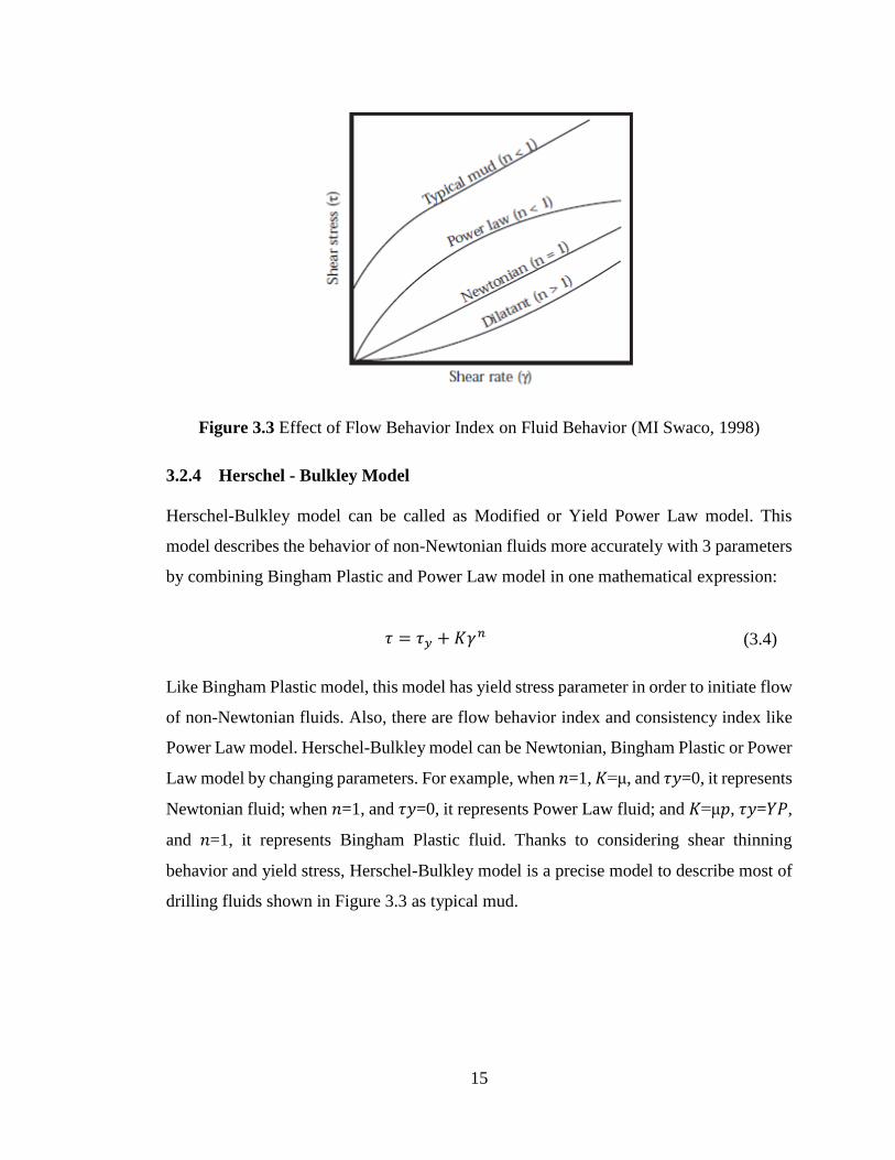
and dilatant fluids when n is bigger than 1. (Figure 3.3) (Rabia, 2001)

15

Figure 3.3 Effect of Flow Behavior Index on Fluid Behavior (MI Swaco, 1998)

3.2.4 Herschel - Bulkley Model

Herschel-Bulkley model can be called as Modified or Yield Power Law model. This

model describes the behavior of non-Newtonian fluids more accurately with 3 parameters

by combining Bingham Plastic and Power Law model in one mathematical expression:

𝜏 = 𝜏𝑦 + 𝐾𝛾𝑛 (3.4)

Like Bingham Plastic model, this model has yield stress parameter in order to initiate flow

of non-Newtonian fluids. Also, there are flow behavior index and consistency index like

Power Law model. Herschel-Bulkley model can be Newtonian, Bingham Plastic or Power

Law model by changing parameters. For example, when 𝑛=1, 𝐾=μ, and 𝜏𝑦=0, it represents

Newtonian fluid; when 𝑛=1, and 𝜏𝑦=0, it represents Power Law fluid; and 𝐾=μ𝑝, 𝜏𝑦=𝑌𝑃,

and 𝑛=1, it represents Bingham Plastic fluid. Thanks to considering shear thinning

behavior and yield stress, Herschel-Bulkley model is a precise model to describe most of

drilling fluids shown in Figure 3.3 as typical mud.

16

3.3 Determination of Rheological Parameters

Our study has also investigated the effect of temperature on parameters of these models

to find a way to describe temperature effect on friction pressure loss. For this reason, it is

important to determine the parameters of models that are interested.

Calculation of model parameters is summarized for Bingham Plastic, Power Law and

Herschel-Bulkley rheological models. (American Petroleum Institute (API), 2009) In

addition to these determination methods, parameters can be found with the relationship

measured shear stresses and shear rates.

3.3.1 Bingham Plastic Model

This model calculates the yield point and plastic viscosity parameters shown in Equation

4.2 by using 600 rpm and 300 rpm dial readings with the formula below.

𝑃𝑙𝑎𝑠𝑡𝑖𝑐 𝑉𝑖𝑠𝑐𝑜𝑠𝑖𝑡𝑦 (𝜇𝑝) = 𝜃600 − 𝜃300 (3.5)

𝑌𝑖𝑒𝑙𝑑 𝑃𝑜𝑖𝑛𝑡 (𝜏𝑦) = 𝜃300 − 𝜇𝑝 (3.6)

Also, the general formula of Bingham-Plastic model shown in Equation 3.2 is used to

determine these parameters. Relationship between shear stress and shear rate is found with

the plot of measured shear stress and shear rates. The slope of the line represents plastic

viscosity and the point intersecting x-axis gives yield point. (MI Swaco, 1998)

3.3.2 Power Law Model

There are two different equations to calculate the flow behavior index (𝑛𝑝) and

consistency index (𝐾𝑝) for pipe and annular flow. Only at high shear rates, the values of

pipe and annulus are accepted as equal. (Bourgoyne Jr. et al., 1991)

17

For pipe flow,

𝐹𝑙𝑜𝑤 𝑏𝑒ℎ𝑎𝑣𝑖𝑜𝑟 𝑖𝑛𝑑𝑒𝑥 (𝑛𝑝) = 3.32 log10 (𝜃600

𝜃300) (3.7)

𝐶𝑜𝑛𝑠𝑖𝑠𝑡𝑒𝑛𝑐𝑦 𝑖𝑛𝑑𝑒𝑥 (𝐾𝑝) =𝜃300

511𝑛𝑝 (3.8)

For annular flow,

𝐹𝑙𝑜𝑤 𝑏𝑒ℎ𝑎𝑣𝑖𝑜𝑟 𝑖𝑛𝑑𝑒𝑥 (𝑛𝑝) = 0.657 log10 (𝜃100

𝜃3) (3.9)

𝐶𝑜𝑛𝑠𝑖𝑠𝑡𝑒𝑛𝑐𝑦 𝑖𝑛𝑑𝑒𝑥 (𝐾𝑝) =𝜃100

170.3𝑛𝑝 (3.10)

Due to exponential relationship of shear stress and shear rate of Power Law fluids, taking

the logarithm of those and then plotting in Cartesian graph gives straight line. The slope

of line represents flow behavior index (𝑛𝑝) and the point intersecting x-axis gives the

logarithm of consistency index (𝐾𝑝). (MI Swaco, 1998)

3.3.3 Herschel-Bulkley Model

Three parameters of Herschel-Bulkley model are determined by following formulas. Yield

stress in this model is known as low shear rate shear stress and calculated with 3 rpm and

6 rpm dial readings of viscometer. Also, flow behavior index and consistency index are

calculated by adding yield point parameters into the equation of Power Law model.

𝑌𝑖𝑒𝑙𝑑 𝑃𝑜𝑖𝑛𝑡 (𝜏𝑦) = 2𝜃3 − 𝜃6 (3.11)

𝐹𝑙𝑜𝑤 𝑏𝑒ℎ𝑎𝑣𝑖𝑜𝑟 𝑖𝑛𝑑𝑒𝑥 (𝑛) = 3.32 log10 (𝜃600 − 𝜏𝑦

𝜃300 − 𝜏𝑦) (3.12)

𝐶𝑜𝑛𝑠𝑖𝑠𝑡𝑒𝑛𝑐𝑦 𝑖𝑛𝑑𝑒𝑥 (𝐾) =𝜃300 − 𝜏𝑦

511𝑛 (3.13)

Herschel-Bulkley model is more different in determination of parameters than Bingham

Plastic and Power Law models since it has three parameters. Therefore, the general

18

formula of this model (Equation 3.4) is linearized by taking the logarithm of both sides of

the equation.

log(𝜏 − 𝜏𝑦) = log 𝐾 + 𝑛 log 𝛾 (3.14)

When log(𝜏 − 𝜏𝑦) vs log 𝛾 is plotted in Cartesian graph, the slope of the straight line gives

flow behavior index and this straight line intersects x-axis at the point of logarithm of

consistency index. (Kelessidis, Maglione, Tsamantaki, and Aspirtakis, 2006) However,

yield point is necessary to plot this graph. The method of Gucuyener (1983) can be used

to find yield point. For this reason, geometric mean of shear rates (𝛾𝐺) is calculated by

minimum (𝛾𝑚𝑖𝑛) and maximum (𝛾𝑚𝑎𝑥) shear rates firstly and corresponding shear stress

(𝜏𝐺) is found for this shear rate.

𝛾𝐺 = √𝛾𝑚𝑖𝑛. 𝛾𝑚𝑎𝑥 (3.15)

Finally, yield stress is calculated with the formula below:

𝜏𝑦 =𝜏𝐺

2 − 𝜏𝑚𝑖𝑛. 𝜏𝑚𝑎𝑥

2𝜏𝐺 − 𝜏𝑚𝑖𝑛 − 𝜏𝑚𝑎𝑥 (3.16)

3.4 Friction Pressure Loss in Annuli

As it is stated in previous sections, friction pressure loss is one of the main issues in

drilling or well completion operations in order to avoid problems arising from inaccurately

prepared hydraulic programs.

In estimation of friction pressure loss in annuli, equation for pipe flow is applied to annular

flow by defining equivalent diameter concepts. (Reed and Pilehvari, 1993) One of the

main aim of this study was to select the most convenient equivalent diameter in friction

pressure loss calculation.

19

The first and mostly known equivalent diameter definition is hydraulic radius concept

that is shown below. It is calculated by four times cross-sectional area of annulus-wetted

perimeter ratio. (Bourgoyne Jr. et al., 1991)

𝐷ℎ𝑦𝑑 = 4 ∗(𝜋 4)⁄ (𝐷𝑜

2 − 𝐷𝑖2)

𝜋(𝐷𝑜 + 𝐷𝑖)= 𝐷𝑜 − 𝐷𝑖 (3.17)

The second definition has been represented by Lamb to explain the friction pressure loss

for laminar flow of Newtonian fluids by considering the flow system as shell of fluid

having radius r. (Lamb, 1945)

𝐷𝐿𝑎𝑚𝑏 = 𝐷𝑜2 + 𝐷𝑖

2 −(𝐷𝑜

2 − 𝐷𝑖2)

ln(𝐷𝑜 𝐷𝑖⁄ ) (3.18)

Another equivalent diameter definition is slot flow approximation. This definition has

been found by comparing different friction pressure loss estimation methods by

representing annulus as a circular and rectangular slot. This concept is applied to annular

geometries having more than 0.3 of the ratio of inner to outer diameter. (Bourgoyne Jr. et

al., 1991)

𝐷𝑠𝑙𝑜𝑡 = 0.816(𝐷𝑜 − 𝐷𝑖) (3.19)

The last definition has been expressed by Crittendon empirically by investigating about a

hundred different field case in fracturing applications. (Crittendon, 1959)

𝐷𝐶𝑟𝑖𝑡 =1

2(√𝐷𝑜

4 − 𝐷𝑖4 −

(𝐷𝑜2 − 𝐷𝑖

2)2

ln(𝐷𝑜 𝐷𝑖⁄ )

4

+ √𝐷𝑜2 − 𝐷𝑖

2) (3.20)

3.4.1 Determination of Friction Pressure Loss in Annuli

Friction pressure loss calculations through concentric annuli are shown in this section

model by considering rheological models for different flow regimes. Newtonian, Bingham

20

Plastic and Power Law models were taken from Applied Drilling Engineering (Bourgoyne

Jr. et al., 1991), and then, Herschel-Bulkley model was solved with methods given in

American Petroleum Institute Recommended Practices 13D: Rheology and Hydraulics of

oil-well drilling fluids (American Petroleum Institute (API), 2009) by considering

concentric annuli. .

3.4.1.1 Newtonian Model

Friction pressure loss can be found by applying Newton’s law of motion to shell of fluid

having radius r. The general equation obtained from this method is:

𝜏 =𝑟

2

𝑑𝑃𝑓

𝑑𝐿+

𝐶

𝑟 (3.21)

where 𝐶 is the integration constant.

Formula stated above is solved for Newtonian model by combining general shear stress-

shear rate relationship of Newtonian fluids expressed in Equation 3.1.

𝜏 = −𝜇𝑑𝑣

𝑑𝑟=

𝑟

2

𝑑𝑃𝑓

𝑑𝐿+

𝐶

𝑟 (3.22)

Velocity obtained from equation by integrating:

𝑣 = −𝑟2

4𝜇

𝑑𝑃𝑓

𝑑𝐿+

𝐶

𝜇ln 𝑟 + 𝐶1 (3.23)

where 𝐶1 is second integration constant.

Equation 4.15 is solved for the boundary conditions representing annulus (𝑟2=inner radius

of outer pipe; 𝑟1=outer radius of inner pipe).Finally, velocity becomes:

𝑣 =1

4𝜇

𝑑𝑃𝑓

𝑑𝐿[(𝑟2

2 − 𝑟2) − (𝑟22 − 𝑟1

2)ln 𝑟2/𝑟

ln 𝑟2/𝑟1] (3.24)

In order to find the relationship between friction pressure loss and flow rate, flow rate is

considered as the total flow of each fluid shell:

21

𝑞 = ∫ 𝑣(2𝜋𝑟)𝑑𝑟 (3.25)

Equation 4.16 is substituted to Equation 3.17 and integrated. Then flow rate is represented

as:

𝑞 =𝜋

8𝜇

𝑑𝑃𝑓

𝑑𝐿[(𝑟2

4 − 𝑟14) −

(𝑟22 − 𝑟1

2)2

ln 𝑟2/𝑟1] = 𝜋(𝑟2

2 − 𝑟12)�̅� (3.26)

As a result, friction pressure loss equation demonstrated below is derived in terms of field

units:

𝑑𝑃𝑓

𝑑𝐿=

𝜇�̅�

1500 (𝐷𝑜2 + 𝐷𝑖

2 −(𝐷𝑜

2 − 𝐷𝑖2)

2

ln 𝐷𝑜/𝐷𝑖)

(3.27)

This equation has been derived by Lamb. (Lamb, 1945) Denominator of this formula

represents equivalent diameter definition of Lamb. Instead of Lamb’s diameter, other

equivalent diameter definitions can be used for Newtonian laminar flow and equation

becomes:

𝑑𝑃𝑓

𝑑𝐿=

𝜇�̅�

1500(𝐷𝑒𝑞)2 (3.28)

Same equation is obtained by representing annulus as a rectangular slot. When slot flow

approximation is used as equivalent diameter, the general formula of this representation

is found.

Average velocity through annulus is calculated with formula below:

�̅� =𝑞

2.448(𝐷𝑜2 − 𝐷𝑖

2) (3.29)

Average velocity is used for all equivalent diameter definition except Crittendon’s

diameter. When Crittendon’s diameter is used, in equation 3.21, (𝐷𝑜2 − 𝐷𝑖

2) is replaced

with 𝐷𝐶𝑟𝑖𝑡2. (Jensen and Sharma, 1987)

22

For turbulent flow, firstly, dimensionless Reynolds number is necessary to determine the

onset of turbulence. Equation of Reynolds number for annular flow is:

𝑁𝑅𝑒 =928𝜌�̅�𝐷𝑒𝑞

𝜇 (3.30)

If Reynolds number exceeds 2100, flow regime is accepted as turbulent. Friction pressure

loss in turbulent conditions is estimated empirically by adding the parameter of friction

factor. The relationship between friction factor and Reynolds number has been presented

by Colebrook (Colebrook, 1939):

1

√𝑓= −4 log(0.269 𝜖 𝐷⁄ +

1.255

𝑁𝑅𝑒√𝑓 ) (3.31)

For smooth pipes (𝜖 𝐷 =⁄ 0) and 2100 ≤ 𝑁𝑅𝑒 ≤ 100000, Blasius has proposed following

equation:

𝑓 =0.0791

𝑁𝑅𝑒0.25 (3.32)

Finally, friction pressure loss equation for annular turbulent flow in terms of field units

becomes:

𝑑𝑃𝑓

𝑑𝐿=

𝑓𝜌�̅�2

25.8𝐷𝑒𝑞 (3.33)

3.4.1.2 Bingham Plastic Model

Friction pressure loss for Bingham Plastic model in laminar flow condition is found by

applying the similar procedure of Newtonian model by using general Bingham Plastic

model equation (Equation 3.2).

𝑑𝑃𝑓

𝑑𝐿=

𝜇𝑝�̅�

1500(𝐷𝑒𝑞)2 +

𝜏𝑦

225𝐷𝑒𝑞 (3.34)

23

The onset of turbulence in Bingham Plastic model is determined by using two criteria.

The first criterion is that turbulence begins when Reynolds number exceeds 2100.

Reynolds number is calculated with Equation 3.22. Apparent viscosity term shown below

is used in general formula of Reynolds number.

𝜇𝑎𝑝𝑝 = 𝜇𝑝 +6.66𝜏𝑦𝐷𝑒𝑞

�̅� (3.35)

The second criterion is to examine Hedstrom number. This number is given as:

𝐻𝑒 =37100𝜌𝜏𝑦𝐷𝑒𝑞

2

𝜇𝑝2

(3.36)

By using Hedstrom number chart, critical Reynolds number is found. This critical number

is compared with calculated Reynolds number by using Equation 3.22 with plastic

viscosity.

After deciding that flow regime is turbulent, friction factor is determined with Colebrook

function and then, friction pressure loss is found by using Equation 3.25.

3.4.1.3 Power Law Model

Friction pressure loss through annulus for Power Law model in laminar flow condition is

calculated by using this formula:

𝑑𝑃𝑓

𝑑𝐿=

𝐾𝑃�̅�𝑛𝑝

144000(𝐷𝑒𝑞)1+𝑛𝑝

(3 + 1/𝑛𝑝

0.0416)

𝑛𝑝

(3.37)

Laminar to turbulent flow regime transition occurs when Reynolds number reaches to

2100. To calculate the Reynolds number, apparent viscosity used in Equation 3.22 is

shown below.

𝜇𝑎𝑝𝑝 =𝐾𝑃𝑑(1−𝑛𝑝)

96�̅�1−𝑛𝑝(

3 + 1/𝑛𝑝

0.0416)

𝑛𝑝

(3.38)

24

Colebrook correlation does not give accurate results in Power Law model. Thus, Dodge

and Metzner, 1959 correlation is used to determine friction factor.

√1

𝑓=

4

𝑛𝑝0.75

log [𝑁𝑅𝑒𝑓(1−𝑛𝑝

2)] −

0.395

𝑛𝑝1.2

(3.39)

Friction pressure loss in turbulent flow regime is calculated with Equation 4.25

3.4.1.4 Herschel – Bulkley Model

Formulas of friction pressure loss for Herschel-Bulkley rheological model has been

derived empirically in API RP 13D for rheology and hydraulics of oil-well drilling fluids

(2009) in laminar, transition and turbulent flow regimes. (American Petroleum Institute

(API), 2009)

Velocity of fluids through annuli is the first parameter to calculate. Following equation

represent velocity of fluid in the unit of ft/min:

�̅� =24.51𝑞

(𝐷𝑜2 − 𝐷𝑖

2) (3.40)

In order to find generalized Reynolds number defined by Metzner and Reed (1955) used

for both pipe and annuli, shear rate and shear stress at pipe wall is necessary. Therefore,

shear rate correction for well geometry to separate pipe and annular flow and viscometer

correction are conducted.

Geometry correction factor is formulated below:

𝐵𝑎 = [(3 − 𝛼)𝑛 + 1

(4 − 𝛼)𝑛] [1 +

𝛼

2] (3.41)

Geometry factor, 𝛼 is accepted as 1 for annular flow.

Viscometer correction factor (𝐵𝑥) is accepted as 1 for Herschel-Bulkley fluids. As a

results, combined geometry shear rate correction factor is calculated by using equation

given as:

25

𝐺 =𝐵𝑎

𝐵𝑥≅ 𝐵𝑎 (3.42)

With this factor, shear rate is determined.

𝛾𝑤 =1.6𝐺𝑉

𝐷𝑒𝑞 (3.43)

After that, shear stress at wall is calculated by combining general Herschel-Bulkley

equation with geometry factor. Equation is shown as:

𝜏𝑤 = 1.066 (4 − 𝛼

3 − 𝛼)

𝑛

𝜏𝑦 + 𝐾𝛾𝑤𝑛 (3.44)

Apparent viscosity of the fluid is determined by dividing wall shear stress to wall shear

rate. (Reed and Pilehvari, 1993) Then, generalized Reynolds number is calculated with

the following equation:

𝑁𝑅𝑒𝐺 =𝜌�̅�2

19.36𝜏𝑤 (3.45)

In order to determine the lower critical Reynolds number for laminar to transition flow

regime, flow behavior index is used.

𝑁𝐶𝑅𝑒,𝐿 = 3470 − 1370𝑛 (3.46)

Upper critical Reynolds number is defined by Schuh (1965) for transition to turbulent flow

regime.

𝑁𝐶𝑅𝑒,𝑈 = 4270 − 1370𝑛 (3.47)

After calculating Reynolds number, friction factor is estimated by combining the

generalized Reynolds number, rheological parameters and flow regimes.

26

For laminar flow, friction factor is calculated as:

𝑓𝑙𝑎𝑚𝑖𝑛𝑎𝑟 =16

𝑁𝑅𝑒𝐺 (3.48)

For transitional flow,

𝑓𝑡𝑟𝑎𝑛𝑠 =16𝑁𝑅𝑒𝐺

𝑁𝐶𝑅𝑒,𝐿2 (3.49)

For turbulent flow, Blasius’ correlation for Power Law model is used.

𝑓𝑡𝑢𝑟𝑏𝑢𝑙𝑒𝑛𝑡 =𝑎

𝑁𝑅𝑒𝐺𝑏 (3.50)

where

𝑎 =log 𝑛𝑝 + 3.93

50

𝑏 =1.75 − log 𝑛𝑝

7

(3.51)

By using friction factors of laminar, transitional and turbulent flow regimes, general

friction factor for all regimes is calculated with the equation shown below:

𝑓 = (𝑓𝑖𝑛𝑡12 + 𝑓𝑙𝑎𝑚𝑖𝑛𝑎𝑟

12)1 12⁄

(3.52)

where

𝑓𝑖𝑛𝑡 = (𝑓𝑡𝑟𝑎𝑛𝑠−8 + 𝑓𝑙𝑢𝑟𝑏𝑢𝑙𝑒𝑛𝑡

−8)8 (3.53)

As a result, friction pressure loss is determined with the given formula:

𝑑𝑃𝑓

𝑑𝐿=

1.076𝜌�̅�2𝑓

105𝐷𝑒𝑞 (3.54)

27

CHAPTER 4

4STATEMENT OF THE PROBLEM

Friction pressure loss is an important parameter for hydraulic program of any well. Factors

affecting friction pressure loss other than temperature have already been investigated by

several researchers. Also, for Newtonian Fluids, a correlation has been proposed for this

effect by using dimensionless parameters. However, temperature effect has not just been

a topic of any research for non-Newtonian fluids.

The primary aim of this study is to investigate the effect of temperature on friction pressure

loss for non-Newtonian fluids through vertical concentric annuli, since, this is a

requirement for drilling in geothermal and HPHT conditions. For this reason, firstly, the

effect of temperature was investigated experimentally by measuring friction pressure loss

and flow rates and then, friction pressure loss was estimated by applying the most suitable

rheological model by considering average error, standard deviation and coefficient of

correlation. And then, theoretical and experimental friction pressure loss results were

compared in order to find the most appropriate equivalent diameter definition. Finally,

model parameters, apparent viscosity and Reynolds number have been examined to see

the temperature effect.

28

29

CHAPTER 5

5EXPERIMENTAL SETUP AND PROCEDURE

Experiments were performed at flow loop laboratory of Middle East Technical University

Department of Petroleum and Natural Gas Engineering. This laboratory has equipment

that are mainly liquid suction and collection tanks, centrifugal pumps, valves to control

flow, flow meter, pressure transmitter and computer program to monitor and save the data.

The aim of the experimental study is to observe the effect of temperature on friction

pressure loss of the flow of water and polymeric drilling fluid including Polyanionic

Cellulose (PAC HV) and Xanthan Gum through the vertical concentric annulus.

Therefore, experiments were divided into two categories:

1- Water experiments

2- Polymeric drilling fluid experiments.

5.1 Experimental Setup

METU PETE Flow loop was modified before conducting experimental works. These

modifications are listed below.

1- Annular test section was brought to a vertical position on its movable corner with

the help of the pulley.

2- In order to increase and monitor the temperature of fluids, resistances and

thermocouples were mounted to suction and cuttings tanks. Also, another

30

thermocouple was mounted to annular test section and connected to a computer to

monitor the temperature of the test section.

3- Two centrifugal mud pumps’ scroll sections were cleaned and fixed to get

maximum performance from the pumps.

4- Since cutting transport were not investigated in experiments, cutting tanks and

lines, and shale shaker were not used and then, return line of fluids was diverted

directly to suction tank.

After all of these modifications, experimental setup was ready to operate. The

schematic of the flow loop is shown in Figure 5.1.

Figure 5.1 Schematic of Flow Loop

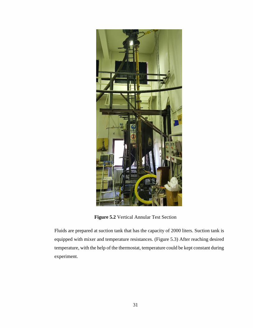
Flow loop has a 21-ft long annular test section including 2.91” ID transparent pipe

with 1.85” OD drill pipe sections demonstrated in Figure 5.2. Eccentricity and rotation

speed of inner pipe can be adjusted. Also, inclination of the pipe is also adjusted from

0 to 90 degree with a movable corner. In this study, experiments were conducted

through a vertical concentric test section with no rotation.

31

Figure 5.2 Vertical Annular Test Section

Fluids are prepared at suction tank that has the capacity of 2000 liters. Suction tank is

equipped with mixer and temperature resistances. (Figure 5.3) After reaching desired

temperature, with the help of the thermostat, temperature could be kept constant during

experiment.

32

Figure 5.3 Mixing motor and Resistances

Fluids prepared in the tank are pumped to the annular test section with two parallel

centrifugal pumps (Figure 5.4), and circulated through the system. The flow rate

control of fluids is provided by a pneumatic valve that adjusted flow rate remotely.

(Figure 5.5).

33

Figure 5.4 Mud Pumps

Figure 5.5 Pneumatic Flow Control Valve

Air is pumped to operate the pneumatic valve by an air compressor. (Figure 5.6) Also,

flow rate is measured by a magnetic flow meter located between pumps and pneumatic

valve. (Figure 5.7)

34

Figure 5.6 Air Compressor

Figure 5.7 Flow meter

There are two pressure taps on annular test section directly enter to pressure transmitter

(Figure 5.8) in order to measure the friction pressure loss of 1 ft section through the

annulus. In this study, lower tap was positioned at 14.9 ft from inlet, and upper tap was

35

located at 5.1 ft from outlet to keep away from end effect and get data from fully developed

section. Lines from the test section and fresh water tap are controlled at the manifold with

several valves. The duties of manifold are to remove air and any contaminants from

transmitter with fresh water and to equalize pressure after conducting experiments.

Figure 5.8 Pressure Transmitter

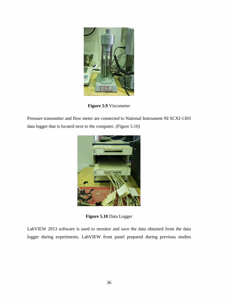
Dial readings at different shear rates are measured with Viscometer shown in Figure 5.9.

In this experiments, dial readings and temperature were measured before pumping to

system and after returning to the liquid tank at steady state.

36

Figure 5.9 Viscometer

Pressure transmitter and flow meter are connected to National Instrument NI SCXI-1303

data logger that is located next to the computer. (Figure 5.10)

Figure 5.10 Data Logger

LabVIEW 2013 software is used to monitor and save the data obtained from the data

logger during experiments. LabVIEW front panel prepared during previous studies

37

performed in this laboratory was used in this study. (Figure 5.11) For accurate

measurement, calibration checks were conducted regularly.

Figure 5.11 LabVIEW Front Panel

The capacity and brand name of equipment in the flow loop are listed in the table below.

Table 5.1 Brand Name and Capacity of Equipment in Laboratory

Equipment Brand Name Capacity

Air Compressor SETKOM SVK 30 3650 lt/min at 8 bar

Centrifugal Pumps DOMAK 1.136 m3/min

Liquid Tank 2000 m3

Magnetic Flow Meter TOSHIBA 1.136 m3/min

Differential Pressure Transducer AUTROL APT 3100 0 – 5 psi

Electro Pneumatic Control Valve SAMSON

Viscometer FANN 35SA

5.2 Procedure

All experiments were started to perform at ambient temperature (about 25°C) and

atmospheric pressure. After that, temperature of the system was increased gradually up to

38

about 45°C. For conducting experiments, annular test section was positioned vertically,

and inner drill pipe was not rotated. To maintain the accuracy of measurements, equipment

was calibrated regularly. As mentioned previously, experiments were divided into two

section named as water and polymeric drilling fluid experiments.

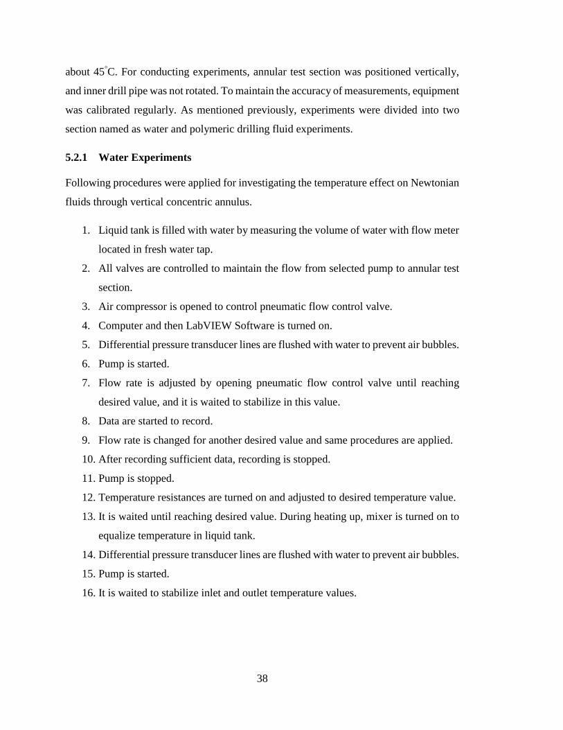
5.2.1 Water Experiments

Following procedures were applied for investigating the temperature effect on Newtonian

fluids through vertical concentric annulus.

1. Liquid tank is filled with water by measuring the volume of water with flow meter

located in fresh water tap.

2. All valves are controlled to maintain the flow from selected pump to annular test

section.

3. Air compressor is opened to control pneumatic flow control valve.

4. Computer and then LabVIEW Software is turned on.

5. Differential pressure transducer lines are flushed with water to prevent air bubbles.

6. Pump is started.

7. Flow rate is adjusted by opening pneumatic flow control valve until reaching

desired value, and it is waited to stabilize in this value.

8. Data are started to record.

9. Flow rate is changed for another desired value and same procedures are applied.

10. After recording sufficient data, recording is stopped.

11. Pump is stopped.

12. Temperature resistances are turned on and adjusted to desired temperature value.

13. It is waited until reaching desired value. During heating up, mixer is turned on to

equalize temperature in liquid tank.

14. Differential pressure transducer lines are flushed with water to prevent air bubbles.

15. Pump is started.

16. It is waited to stabilize inlet and outlet temperature values.

39

17. After reaching desired temperature value, flow rate is adjusted by opening

pneumatic flow control valve until reaching desired flow rate value, and it is

waited to stabilize in this value.

18. Same steps (8 to 17) are applied for all temperature values.

19. Pump and then air compressor are stopped after all experiments are conducted.

Test matrix for water experiments is shown Table 5.2.

Table 5.2 Test Matrix for Water Experiments

Minimum – Maximum

Average Liquid Flow Rate 40 – 110 gpm

Temperature 20 – 45°C

5.2.2 Polymeric Drilling Fluid Experiments

Polymeric drilling fluid experiments are categorized as drilling fluid preparation and

experiments.

5.2.2.1 Fluid Preparation

Polymeric drilling fluid was prepared with REOPAC HV (Polyanionic Cellulose) and

REOZAN D (Xanthan Gum) provided by GEOS Energy Inc (Figure 5.12).

40

Figure 5.12 Drilling Fluid Additives

REOPAC HV is used as viscosifier and fluid loss control additive, and REOZAN D is

used as viscosifier in industry. Before starting experimental works in flow loop, the

amount of these additives were determined as 0.50 and 0.75 lb/bbl for REOPAC HV and

REOZAN D, respectively in Middle East Technical University Department of Petroleum

and Natural Gas Engineering Drilling Fluid Laboratory. Physical properties of these

additives taken from GEOS Energy Inc. are listed below.

Table 5.3 Physical Properties of Additives

REOZAN-D REOPAC HV

Appearance Cream colored powder White powder

pH 6-8 (1% solution) 7-8 (1% solution)

Bulk Density (kg/m3) 650-900 600-800

Following procedures were applied for preparation of drilling fluid.

1. Liquid tank is filled with water (1200 lt).

2. Mixer is turned on.

41

3. Pump is started and flow is directed to bypass line to avoid occurring fisheye

during polymeric fluid preparation.

4. REOPAC HV and REOZAN D are added to the water very slowly in amount of

0.10 lb/bbl, respectively.

5. After adding desired amount of these additives, dial readings are measured and

recorded.

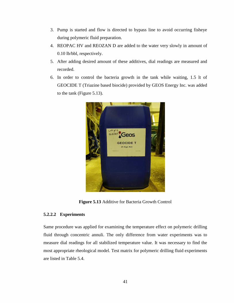
6. In order to control the bacteria growth in the tank while waiting, 1.5 lt of

GEOCIDE T (Triazine based biocide) provided by GEOS Energy Inc. was added

to the tank (Figure 5.13).

Figure 5.13 Additive for Bacteria Growth Control

5.2.2.2 Experiments

Same procedure was applied for examining the temperature effect on polymeric drilling

fluid through concentric annuli. The only difference from water experiments was to

measure dial readings for all stabilized temperature value. It was necessary to find the

most appropriate rheological model. Test matrix for polymeric drilling fluid experiments

are listed in Table 5.4.

42

Table 5.4 Test Matrix for Polymeric Drilling Fluid Experiments

Minimum – Maximum

Average Liquid Flow Rate 25 – 110 gpm

Temperature 24 – 44°C

43

CHAPTER 6

6RESULTS AND DISCUSSION

6.1 Water Experiments

Experiments with water were conducted to see the effect of temperature on the flow of

Newtonian fluids in vertical concentric annulus. Calculations for friction pressure loss

through annulus were performed by applying Newtonian model explained in Theory

section with the effect of equivalent diameter concepts. (Bourgoyne Jr. et al., 1991) For

this reason, for four different temperatures (20, 25, 35 and 45°C), friction pressure losses

through annulus were estimated separately with equivalent diameter definitions of

hydraulic radius (HR), slot flow approximation (SA), Lamb’s (LC) and Crittendon’s (CC)

diameter.

Density and viscosity of water and diameter calculated with equivalent diameter concepts

are listed below.

Table 6.1 Properties of Water (Bourgoyne Jr. et al., 1991)

Temperature (°C) 20 25 35 45

Density (ppg) 8.3304 8.3208 8.2956 8.2637

Viscosity (cp) 1.0005 0.8891 0.7198 0.5970

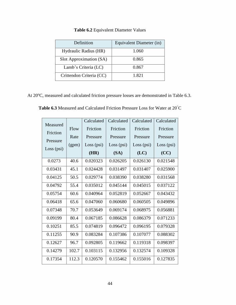
44

Table 6.2 Equivalent Diameter Values

Definition Equivalent Diameter (in)

Hydraulic Radius (HR) 1.060

Slot Approximation (SA) 0.865

Lamb’s Criteria (LC) 0.867

Crittendon Criteria (CC) 1.821

At 20oC, measured and calculated friction pressure losses are demonstrated in Table 6.3.

Table 6.3 Measured and Calculated Friction Pressure Loss for Water at 20°C

Measured

Friction

Pressure

Loss (psi)

Flow

Rate

(gpm)

Calculated

Friction

Pressure

Loss (psi)

(HR)

Calculated

Friction

Pressure

Loss (psi)

(SA)

Calculated

Friction

Pressure

Loss (psi)

(LC)

Calculated

Friction

Pressure

Loss (psi)

(CC)

0.0273 40.6 0.020323 0.026205 0.026130 0.021548

0.03431 45.1 0.024428 0.031497 0.031407 0.025900

0.04125 50.5 0.029774 0.038390 0.038280 0.031568

0.04792 55.4 0.035012 0.045144 0.045015 0.037122

0.05754 60.6 0.040964 0.052819 0.052667 0.043432

0.06418 65.6 0.047060 0.060680 0.060505 0.049896

0.07348 70.7 0.053649 0.069174 0.068975 0.056881

0.09199 80.4 0.067185 0.086628 0.086379 0.071233

0.10251 85.5 0.074819 0.096472 0.096195 0.079328

0.11255 90.9 0.083284 0.107386 0.107077 0.088302

0.12627 96.7 0.092805 0.119662 0.119318 0.098397

0.14279 102.7 0.103115 0.132956 0.132574 0.109328

0.17354 112.3 0.120570 0.155462 0.155016 0.127835

45

Following graph (Figure 6.1) is given to represent these friction pressure loss vs. flow rate

plot.

As it can be seen in Figure 6.1, measured friction pressure loss through annulus gave the

results with the best agreement with slot approximation and Lamb’s diameter. In order to

investigate the effect of temperature, graph of measured pressure loss vs. Reynolds

number calculated with slot approximation was examined at 20, 25, 35 and 45°C. It is

demonstrated in Figure 6.2. Results for 25, 35 and 45°C are shown in Appendix.

Figure 6.1 Friction Pressure Loss vs. Flow Rate at 20°C

As Reynolds number increased, the difference in friction pressure loss became more

distinct with increasing temperature. This was related with viscosity and density terms in

the formula of Reynolds number. The denominator of the Reynolds number formula

decreased more significantly than the numerator with temperature and this caused the

difference in friction pressure losses. Also, friction pressure loss increased with Reynolds

number for all temperatures but this increase became more pronounced at lower

temperature. Regime transition with temperature effect could not be examined due to

critical flow rate for transition was very low to be achieved with this experimental setup.

0

0,02

0,04

0,06

0,08

0,1

0,12

0,14

0,16

0,18

0,2

0 20 40 60 80 100 120

Fri

ctio

n P

ress

ure

Lo

ss (

psi

)

Flow Rate (gpm)

Friction Pressure Loss vs. Flow Rate

HR

SA

LC

CC

Experiment

46

Figure 6.2 Friction Pressure Loss vs. Reynolds Number for Water

.

0

0,02

0,04

0,06

0,08

0,1

0,12

0,14

0,16

0,18

0,2

0 20000 40000 60000 80000 100000 120000

Fri

ctio

n P

ress

ure

Lo

ss (

psi

)

Reynolds Number

Friction Pressure Loss vs. Reynolds Number

20 C

25 C

35 C

45 C

47

6.2 Polymeric Drilling Fluid Experiments

Experiments conducted by using polymeric drilling fluids were divided into two parts that

were rheological measurements and friction pressure loss measurements. Results obtained

from rheological measurements were used to find the most suitable rheological model for

drilling fluids. Then, friction pressure losses through vertical concentric annular test

section were determined with the selected model theoretically. All processes were

repeated for all temperatures. Results from friction pressure loss experiments were used

to compare with theoretical results to investigate the effect of temperature on the annular

flow of polymeric drilling fluid.

6.2.1 Rheological Measurements

Rheological parameters for Bingham Plastic, Power Law and Herschel-Bulkley models

were calculated by using dial readings at 600, 300, 200, 100, 6 and 3 rpm from viscometer

during experiments with polymeric drilling fluid for different temperatures when reaching

steady state.

Following table demonstrates all results obtained from viscometer measurements.

Table 6.4 Viscometer Dial Readings

Viscometer Speed

(RPM)

Dial

Reading

24oC

Dial

Reading

30oC

Dial

Reading

37oC

Dial

Reading

44oC

600 27 24 21 18.5

300 19.5 17 16 13.5

200 16 15 13 11.5

100 12 11 10 8.5

6 4.5 4 3.5 3

3 3.5 3 3 2.5

48

As mentioned previously in Theory section of thesis, relationship between shear stress

and shear rate should be examined to determine rheological parameters. After that,

theoretically obtained shear stress values by using determined parameters were compared

with measured ones for each model statistically and values of average error, standard

deviation and coefficient of determination (R2) were found with following formulas.

𝐸𝑟𝑟𝑜𝑟 =𝜏𝑚𝑒𝑎𝑠𝑢𝑟𝑒𝑑 − 𝜏𝑐𝑎𝑙𝑐𝑢𝑙𝑎𝑡𝑒𝑑

𝜏𝑚𝑒𝑎𝑠𝑢𝑟𝑒𝑑∗ 100 (6.1)

𝑆𝑡𝑎𝑛𝑑𝑎𝑟𝑑 𝐷𝑒𝑣𝑖𝑎𝑡𝑖𝑜𝑛 = √|𝜏𝑐𝑎𝑙𝑐𝑢𝑙𝑎𝑡𝑒𝑑 − 𝜏𝑐𝑎𝑙𝑐𝑢𝑙𝑎𝑡𝑒𝑑̅̅ ̅̅ ̅̅ ̅̅ ̅̅ ̅̅ ̅|2

5 (6.2)

At 24oC, firstly, Bingham Plastic model was investigated. For this reason, measured shear

stress vs. shear rate graph shown in Figure 6.3 were plotted.

According to this graph, the slope of straight line and intersection point with x-axis gave

plastic viscosity (𝜇𝑝) and yield point (𝜏𝑦), respectively. These values were used to

determine shear stress theoretically. Table 6.5 and 6.6 shows results for Bingham Plastic

model at 24oC.

49

Figure 6.3 Measured Shear Stress vs. Shear Rate Graph at 24°C

Table 6.5 Measured and Calculated Shear Stress Values for Bingham Plastic Model at

24°C

Viscometer Speed

(RPM)

Shear

Rate

(1/sec)

Dial

Reading

Measured

Shear Stress

(lb/100ft2)

Calculated

Shear Stress

(lb/100ft2)

Error (%)

600 1021.80 27 28.83 31.05 7.70

300 510.90 19.5 20.82 18.73 10.06

200 340.60 16 17.08 14.62 14.42

100 170.30 12 12.81 10.51 17.95

6 10.22 4.5 4.81 6.65 38.44

3 5.11 3.5 3.74 6.53 74.70

Av. Error 27.21

St. Deviation 9.30

R2 0.9314

y = 0,0241x + 6,406

R² = 0,9314

0,00

5,00

10,00

15,00

20,00

25,00

30,00

35,00

0,00 200,00 400,00 600,00 800,00 1000,00 1200,00

Shea

r S

tres

s (l

b/1

00

ft2)

Shear Rate (1/sec)

Shear Stress vs. Shear Rate

50

Table 6.6 Bingham Plastic Model Parameters at 24°C

µp (lb-s/100ft2) 0.02

τy (lb/100ft2) 6.41

Power Law model parameters at 24°C were determined by plotting the graph of logarithm

of measured shear stress vs. logarithm of shear rate. (Figure 6.4)

Figure 6.4 Log of Shear Stress vs. Log of Shear Rate Graph at 24°C

The slope of straight line obtained from graph gave flow behavior index (𝑛𝑝) and

intersection point with x-axis gave the logarithm of consistency index (𝐾𝑝). Table 6.7 and

6.8 demonstrates results for Power Law rheological model at 24°C.

y = 0,3763x + 0,2971

R² = 0,9966

0,00

0,20

0,40

0,60

0,80

1,00

1,20

1,40

1,60

0,00 0,50 1,00 1,50 2,00 2,50 3,00 3,50

log o

f S

hea

r S

tres

s

log of Shear Rate

log (Shear Stress) vs. log (Shear Rate)

51

Table 6.7 Measured and Calculated Shear Stress Values for Power Law Model at 24°C

Viscometer Speed

(RPM)

Shear Rate

(1/sec)

Dial

Reading

Measured

Shear Stress

(lb/100ft2)

Calculated

Shear Stress

(lb/100ft2)

Error

(%)

600 1021.80 27 28.83 26.89 6.75

300 510.90 19.5 20.82 20.71 0.53

200 340.60 16 17.08 17.78 4.08

100 170.30 12 12.81 13.70 6.91

6 10.22 4.5 4.81 4.75 1.10

3 5.11 3.5 3.74 3.66 2.04

Av. Error 3.57

St. Deviation 9.12

R2 0.9966

Table 6.8 Power Law Model Parameters at 24°C

Flow Behavior Index (np) 0.38

Consistency Index (Kp) (lb-secn/100 ft2) 1.98

Herschel-Bulkley model parameters at 24°C were found by using GRG Nonlinear Solving

method in SOLVER add-in of Microsoft Excel because of the complexity of three

parameters. In order to apply SOLVER function, initial values of parameters were

determined by plotting the graph of logarithm of measured shear stress minus yield stress

vs logarithm of shear rate. To plot this graph, firstly, yield point was found by Gucuyener’s

method. (Gucuyener, 1983) Then, like Power Law model, the slope of straight line

obtained from graph gave the flow behavior index (n) and intersection point with x-axis

gave the logarithm of consistency index (K). Following table shows the initial values of

model parameters and figure shows the graph of logarithm of measured shear stress minus

yield stress vs logarithm of shear rate.

52

Table 6.9 Initial Values of Herschel-Bulkley Parameters

Shear Rate (Geometric Mean) (γG) (1/sec) 72.25

Shear Stress at Geo. Mean of Shear Rate (τG) (lb/100ft2) 7.44

Yield Point (τy) (lb/100ft2) 2.96

Flow Behavior Index (n) 0.64

Consistency Index (K) (lb-secn/100 ft2) 0.34

Figure 6.5 Log of Shear Stress vs. Log of Shear Rate Graph for Initial Parameters at

24°C

SOLVER found the optimum Herschel-Bulkley model parameters by minimizing the

square of difference between calculated and measured shear stress values. According to

results, table of measured and calculated shear stresses, the graph of logarithm of

measured shear stress minus yield stress vs logarithm of shear rate and table of model

parameters are shown below.

y = 0,6373x - 0,4682

R² = 0,9893

-0,20

0,00

0,20

0,40

0,60

0,80

1,00

1,20

1,40

1,60

0,00 0,50 1,00 1,50 2,00 2,50 3,00 3,50

log o

f S

hea

r S

tres

s -

Yie

ld P

oin

t

log of Shear Rate

log(Shear Stress - Yield Point) vs log(Shear Rate)

53

Table 6.10 Measured and Calculated Shear Stress Values for Herschel-Bulkley Model at

24°C

Viscometer Speed

(RPM)

Shear Rate

(1/sec)

Dial

Reading

Measured

Shear Stress

(lb/100ft2)

Calculated

Shear Stress

(lb/100ft2)

Error

(%)

600 1021.80 27 28.83 28.81 0.08

300 510.90 19.5 20.82 20.78 0.20

200 340.60 16 17.08 17.26 1.02

100 170.30 12 12.81 12.71 0.78

6 10.22 4.5 4.81 4.64 3.49

3 5.11 3.5 3.74 3.90 4.29

Av. Error 1.64

St. Deviation 9.64

R2 0.998

54

Figure 6.6 Log of Shear Stress vs. Log of Shear Rate Graph for SOLVER Parameters at

24°C

Table 6.11 Herschel-Bulkley Model Parameters at 24°C

Yield Point (τy) 2.18

Flow Behavior Index (n) 0.52

Consistency Index (K) 0.74

Procedures to determine rheological parameters and values of average error, standard

deviation and coefficient of determination at 24°C were applied to other temperatures for

each model. Following tables shows all results for 24, 30, 37 and 44 degrees Celsius.

y = 0,5235x - 0,1467

R² = 0,998

0,00

0,20

0,40

0,60

0,80

1,00

1,20

1,40

1,60

0,00 0,50 1,00 1,50 2,00 2,50 3,00 3,50

log(S

hea

r S

tres

s -

Yie

ld P

oin

t)

log(Shear Rate)

log(Shear Stress - Yield Point) vs log(Shear Rate)

55

Table 6.12 Model Parameters at 24°C

Bingham Plastic

Model

Power Law

Model

Herschel-Bulkley

Model

Average Error 27.21 3.57 1.64

Standard Deviation 9.30 9.12 9.64

R2 0.9314 0.9966 0.9980

Plastic Viscosity (µp) 0.02

Yield Point (τy) 6.41 2.18

Flow Behavior Index (n, np) 0.38 0.52

Consistency Index (K) 1.98 0.74

Table 6.13 Model Parameters at 30°C

Bingham Plastic

Model

Power Law

Model

Herschel-Bulkley

Model

Average Error 30.19 2.44 2.51

Standard Deviation 8.22 8.30 8.58

R2 0.9175 0.9984 0.9979

Plastic Viscosity (µp) 0.02

Yield Point (τy) 5.85 1.44

Flow Behavior Index (n, np) 0.38 0.48

Consistency Index (K) 1.72 0.89

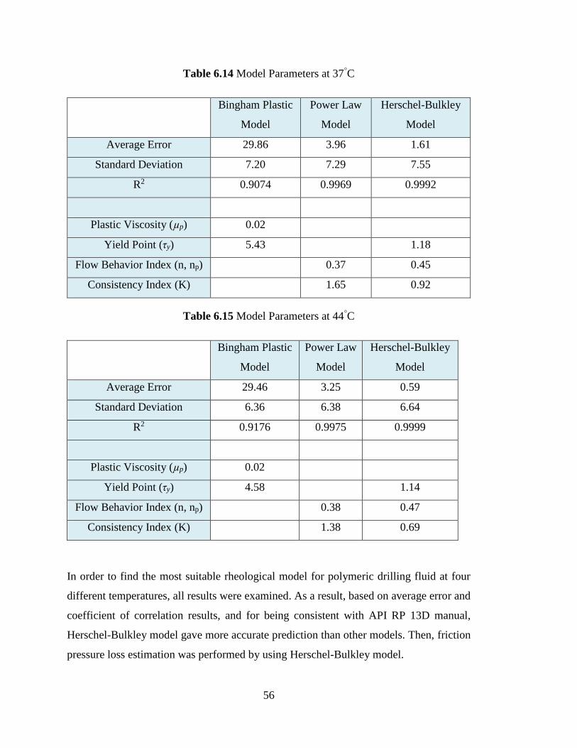
56

Table 6.14 Model Parameters at 37°C

Bingham Plastic

Model

Power Law

Model

Herschel-Bulkley

Model

Average Error 29.86 3.96 1.61

Standard Deviation 7.20 7.29 7.55

R2 0.9074 0.9969 0.9992

Plastic Viscosity (µp) 0.02

Yield Point (τy) 5.43 1.18

Flow Behavior Index (n, np) 0.37 0.45

Consistency Index (K) 1.65 0.92

Table 6.15 Model Parameters at 44°C

Bingham Plastic

Model

Power Law

Model

Herschel-Bulkley

Model

Average Error 29.46 3.25 0.59

Standard Deviation 6.36 6.38 6.64

R2 0.9176 0.9975 0.9999

Plastic Viscosity (µp) 0.02

Yield Point (τy) 4.58 1.14

Flow Behavior Index (n, np) 0.38 0.47

Consistency Index (K) 1.38 0.69

In order to find the most suitable rheological model for polymeric drilling fluid at four

different temperatures, all results were examined. As a result, based on average error and

coefficient of correlation results, and for being consistent with API RP 13D manual,

Herschel-Bulkley model gave more accurate prediction than other models. Then, friction

pressure loss estimation was performed by using Herschel-Bulkley model.

57

6.2.2 Friction Pressure Loss Estimation

After choosing rheological model and determining rheological parameters, friction

pressure losses were calculated with Herschel-Bulkley model. Friction pressure loss for

concentric annular flow is estimated by considering equivalent diameter concepts

mentioned in Theory section. In this study, friction pressure losses were estimated by

applying different equivalent diameter concepts in Herschel-Bulkley model and the most

suitable definition was chosen.

American Petroleum Institute Recommended Practice 13D for Rheology and Hydraulics

of oil-well drilling fluids has represented the methodology for friction pressure loss

estimation through annuli by applying Herschel-Bulkley rheological model. (American

Petroleum Institute (API), 2009) As previously shown in Theory section, hydraulic radius

concept has been used in calculation in API RP 13D. In this study, other equivalent

diameter definitions named as slot flow approximation, Lamb’s criteria and Crittendon’s

criteria were added to formulas instead of hydraulic radius, and friction pressure losses

were calculated. The values of equivalent diameter for four different equivalent diameter

concepts were shown in Table 6.2 previously.

Also, API RP 13D stated that Herschel-Bulkley model parameters were calculated with

field measurements directly by using Equation 3.3, 3.4 and 3.5. However, in this study, in

calculation of friction pressure loss, model parameters were obtained from SOLVER

results. Since, average error value with parameters from field measurements was more

than SOLVER results at 24oC. (Table 6.16)

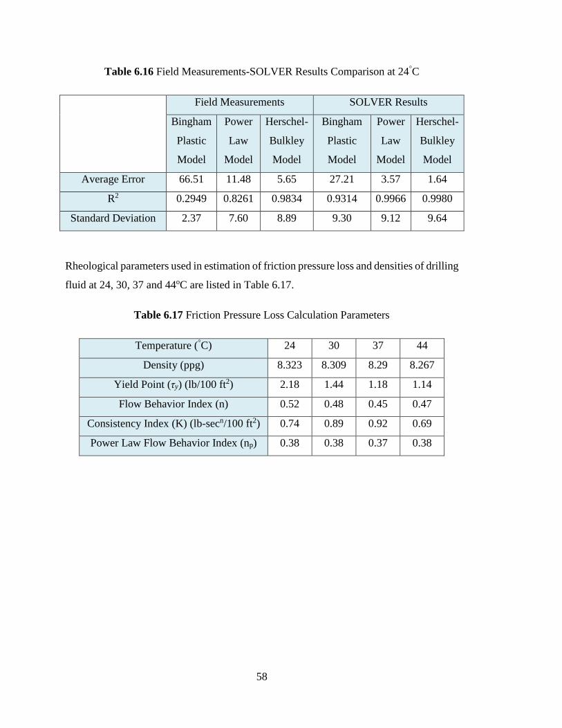
58

Table 6.16 Field Measurements-SOLVER Results Comparison at 24°C

Field Measurements SOLVER Results

Bingham

Plastic

Model

Power

Law

Model

Herschel-

Bulkley

Model

Bingham

Plastic

Model

Power

Law

Model

Herschel-

Bulkley

Model

Average Error 66.51 11.48 5.65 27.21 3.57 1.64

R2 0.2949 0.8261 0.9834 0.9314 0.9966 0.9980

Standard Deviation 2.37 7.60 8.89 9.30 9.12 9.64

Rheological parameters used in estimation of friction pressure loss and densities of drilling

fluid at 24, 30, 37 and 44oC are listed in Table 6.17.

Table 6.17 Friction Pressure Loss Calculation Parameters

Temperature (°C) 24 30 37 44

Density (ppg) 8.323 8.309 8.29 8.267

Yield Point (τy) (lb/100 ft2) 2.18 1.44 1.18 1.14

Flow Behavior Index (n) 0.52 0.48 0.45 0.47

Consistency Index (K) (lb-secn/100 ft2) 0.74 0.89 0.92 0.69

Power Law Flow Behavior Index (np) 0.38 0.38 0.37 0.38

59

For 24oC, measured friction pressure loss and flow rate values are demonstrated below.

Table 6.18 Measured Friction Pressure Loss and Flow Rate Values at 24°C

P (psi) Q (gpm)

0.0428 25.4

0.05554 30.4

0.05998 35.6

0.06717 40.5

0.07324 45.5

0.08024 50.4

0.08666 55.2

0.09865 60.8

0.11686 70.8

0.12041 75.5

0.12908 90.4

0.1378 95.5

0.16122 110.2

Despite all steps of calculation are shown in Theory, the procedure to find friction pressure

loss is repeated. By using flow rates values, firstly, average velocity through annulus was

calculated for all equivalent diameter concepts by using Equation 3.32 (Table 6.19).

60

Table 6.19 Average Velocities

Q

(gpm)

Average Velocity (Va) (ft/min)

HR, SA, LC CC

25.4 123.39 187.77

30.4 147.67 224.73

35.6 172.93 263.17

40.5 196.74 299.39

45.5 221.03 336.36

50.4 244.83 372.58

55.2 268.14 408.06

60.8 295.35 449.46

70.8 343.93 523.38

75.5 366.76 558.13

90.4 439.14 668.28

95.5 463.91 705.98

110.2 535.32 814.65

Then, combined geometry shear rate correction factor (G) was calculated as 1.9659 (Eq.

3.34) and used in finding shear rates at wall (Eq. 3.35). By using Herschel-Bulkley model

formula, shear stresses at wall were determined (Eq. 3.36). Shear stresses and shear rates

at wall are shown in Table 6.20.

61

Table 6.20 Wall Shear Rates and Shear Stresses at 24°C

Q

(gpm)

WALL SHEAR RATE (1/sec) WALL SHEAR STRESS (lb/100ft2)

γw (HR) γw (SA) γw (LC) γw (CC) τw (HR) τw (SA) τw (LC) τw (CC)

25.4 366.14 448.70 447.67 324.36 19.55 21.41 21.38 18.54

30.4 438.21 537.03 535.79 388.21 21.18 23.21 23.19 20.07

35.6 513.17 628.89 627.44 454.62 22.74 24.95 24.92 21.53

40.5 583.80 715.45 713.80 517.19 24.11 26.47 26.44 22.82

45.5 655.88 803.77 801.92 581.04 25.43 27.94 27.91 24.06

50.4 726.51 890.33 888.28 643.62 26.66 29.30 29.27 25.21

55.2 795.70 975.13 972.88 704.91 27.80 30.57 30.54 26.29

60.8 876.43 1074.05 1071.58 776.43 29.08 31.99 31.96 27.49

70.8 1020.58 1250.71 1247.83 904.13 31.23 34.38 34.34 29.51

75.5 1088.33 1333.73 1330.66 964.15 32.19 35.45 35.41 30.41

90.4 1303.11 1596.95 1593.27 1154.43 35.06 38.63 38.59 33.10

95.5 1376.62 1687.04 1683.16 1219.55 35.99 39.66 39.62 33.97

110.2 1588.52 1946.72 1942.24 1407.28 38.53 42.49 42.44 36.37

After that, lower critical Reynolds number for laminar to transition flow regime and upper

critical Reynolds number for transition to turbulent flow regime were found as 2761 and

3561, respectively (Eq. 3.38, 3.39), and generalized Reynolds numbers were calculated

(Eq. 3.37) and then, friction factor values were estimated (Eq. 3.44) and tabulated in Table

6.21.

62

Table 6.21 Generalized Reynolds Number and Friction Factor at 24°C

Q

(gpm)

GENERALIZED REYNOLDS

NUMBER FRICTION FACTOR

NReG

(HR)

NReG

(SA)

NReG

(LC)

NReG

(CC) f (HR) f (SA) f (LC) f (CC)

25.4 335 306 306 818 0.048 0.052 0.052 0.020

30.4 443 404 404 1082 0.036 0.040 0.040 0.015

35.6 565 515 516 1383 0.028 0.031 0.031 0.012

40.5 690 629 629 1689 0.023 0.025 0.025 0.009

45.5 826 752 753 2022 0.019 0.021 0.021 0.008

50.4 967 880 880 2367 0.017 0.018 0.018 0.007

55.2 1112 1011 1012 2723 0.014 0.016 0.016 0.006

60.8 1289 1172 1173 3159 0.012 0.014 0.014 0.006

70.8 1628 1479 1481 3991 0.010 0.011 0.011 0.005

75.5 1796 1631 1633 4404 0.009 0.010 0.010 0.005

90.4 2365 2146 2148 5800 0.007 0.007 0.007 0.005

95.5 2571 2333 2335 6307 0.006 0.007 0.007 0.005

110.2 3197 2899 2903 7846 0.006 0.006 0.006 0.004

Calculated friction pressure losses for four different equivalent diameter concept are listed

in Table 6.22 (Eq. 3.45). Results of other temperatures are listed in Appendix.

63

Table 6.22 Calculated Friction Pressure Losses at 24°C

Q

(gpm)

FRICTION PRESSURE LOSS

(psi/ft)

dPf/dL

(HR)

dPf/dL

(SA)

dPf/dL

(LC)

dPf/dL

(CC)

25.4 0.0615 0.0825 0.0822 0.0339

30.4 0.0666 0.0894 0.0891 0.0367

35.6 0.0715 0.0961 0.0958 0.0394

40.5 0.0758 0.1020 0.1017 0.0418

45.5 0.0800 0.1076 0.1073 0.0440

50.4 0.0838 0.1129 0.1125 0.0462

55.2 0.0874 0.1178 0.1174 0.0493

60.8 0.0914 0.1233 0.1229 0.0564

70.8 0.0982 0.1325 0.1320 0.0718

75.5 0.1012 0.1366 0.1361 0.0793

90.4 0.1104 0.1489 0.1484 0.1043

95.5 0.1142 0.1530 0.1525 0.1135

110.2 0.1371 0.1730 0.1725 0.1412

Graphical representation of measured and estimated friction pressure losses for 24, 30, 37

and 44°C are demonstrated in Figure 6.7, 6.8, 6.9, 6.10.

64

Figure 6.7 Measured and Calculated Friction Pressure Loss vs. Flow Rate at 24°C

Figure 6.8 Measured and Calculated Friction Pressure Loss vs. Flow Rate at 30°C

0

0,02

0,04

0,06

0,08

0,1

0,12

0,14

0,16

0,18

0,2

0 20 40 60 80 100 120

Fri

ctio

n P

ress

ure

Lo

ss (

psi

)

Flow Rate (gpm)

Friction Pressure Loss vs Flow Rate

Experiment

HR

SA

LC

CC

0

0,02

0,04

0,06

0,08

0,1

0,12

0,14

0,16

0,18

0,2

0 20 40 60 80 100 120

Fri

ctio

n P

ress

ure

Lo

ss (

psi

)

Flow Rate (gpm)

Friction Pressure Loss vs Flow Rate

Experiment

HR

SA

LC

CC

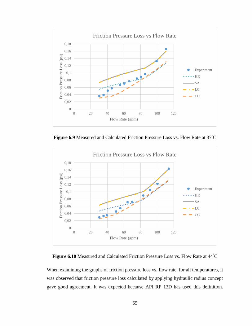
65

Figure 6.9 Measured and Calculated Friction Pressure Loss vs. Flow Rate at 37°C

Figure 6.10 Measured and Calculated Friction Pressure Loss vs. Flow Rate at 44°C

When examining the graphs of friction pressure loss vs. flow rate, for all temperatures, it

was observed that friction pressure loss calculated by applying hydraulic radius concept

gave good agreement. It was expected because API RP 13D has used this definition.

0

0,02

0,04

0,06

0,08

0,1

0,12

0,14

0,16

0,18

0 20 40 60 80 100 120

Fri

ctio

n P

ress

ure

Lo

ss (

psi

)

Flow Rate (gpm)

Friction Pressure Loss vs Flow Rate

Experiment

HR

SA

LC

CC

0

0,02

0,04

0,06

0,08

0,1

0,12

0,14

0,16

0,18

0 20 40 60 80 100 120

Fri

ctio

n P

ress

ure

Lo

ss (

psi

)

Flow Rate (gpm)

Friction Pressure Loss vs Flow Rate

Experiment

HR

SA

LC

CC

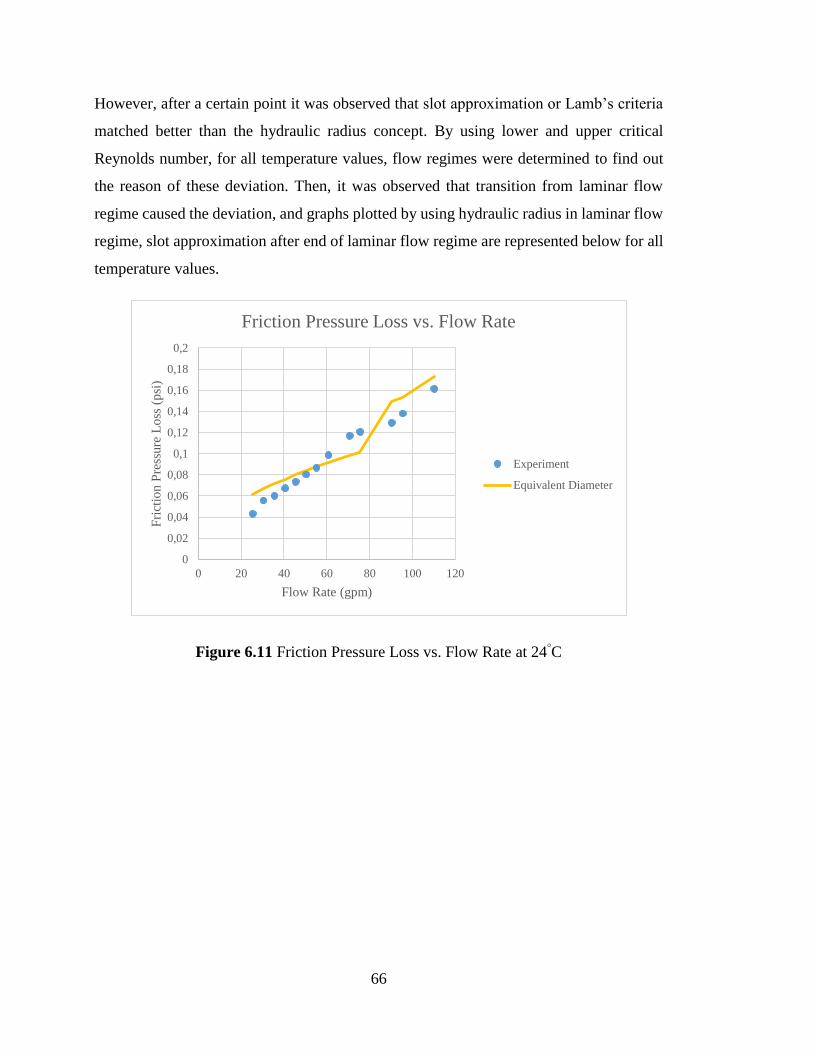
66

However, after a certain point it was observed that slot approximation or Lamb’s criteria

matched better than the hydraulic radius concept. By using lower and upper critical

Reynolds number, for all temperature values, flow regimes were determined to find out

the reason of these deviation. Then, it was observed that transition from laminar flow

regime caused the deviation, and graphs plotted by using hydraulic radius in laminar flow

regime, slot approximation after end of laminar flow regime are represented below for all

temperature values.

Figure 6.11 Friction Pressure Loss vs. Flow Rate at 24°C

0

0,02

0,04

0,06

0,08

0,1

0,12

0,14

0,16

0,18

0,2

0 20 40 60 80 100 120

Fri

ctio

n P

ress

ure

Lo

ss (

psi

)

Flow Rate (gpm)

Friction Pressure Loss vs. Flow Rate

Experiment

Equivalent Diameter

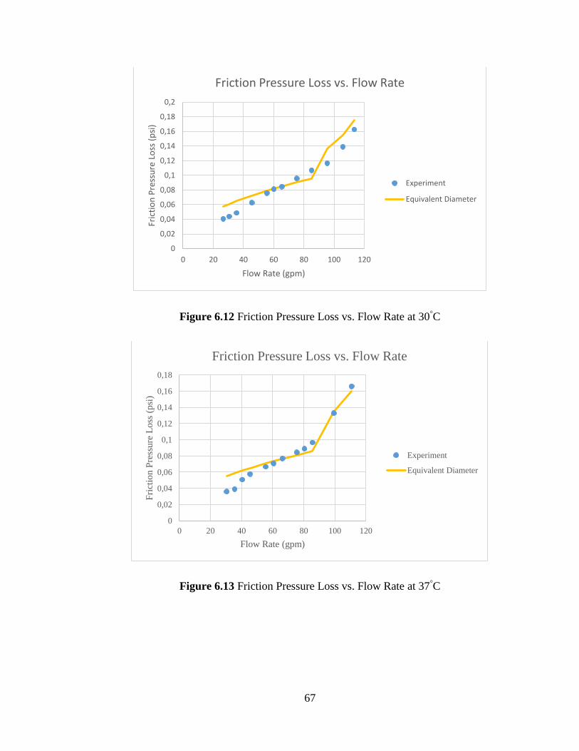
67

Figure 6.12 Friction Pressure Loss vs. Flow Rate at 30°C

Figure 6.13 Friction Pressure Loss vs. Flow Rate at 37°C

0

0,02

0,04

0,06

0,08

0,1

0,12

0,14

0,16

0,18

0,2

0 20 40 60 80 100 120

Fric

tio

n P

ress

ure

Lo

ss (

psi

)

Flow Rate (gpm)

Friction Pressure Loss vs. Flow Rate

Experiment

Equivalent Diameter

0

0,02

0,04

0,06

0,08

0,1

0,12

0,14

0,16

0,18

0 20 40 60 80 100 120

Fri

ctio

n P

ress

ure

Lo

ss (

psi

)

Flow Rate (gpm)

Friction Pressure Loss vs. Flow Rate

Experiment

Equivalent Diameter

68

Figure 6.14 Friction Pressure Loss vs. Flow Rate at 44°C

0

0,02

0,04

0,06

0,08

0,1

0,12

0,14

0,16

0,18

0 20 40 60 80 100 120

Fri

ctio

n P

ress

ure

Lo

ss (

psi

)

Flow Rate (gpm)

Friction Pressure Loss vs. Flow Rate

Experiment

Equivalent Diameter

69

6.3 Investigation of Temperature Effect

In order to examine temperature effect on friction pressure loss through the annulus, the

components of the friction pressure loss calculation were investigated. For this reason,

Relationships of Herschel-Bulkley parameters (yield point, flow behavior index and

consistency index), apparent viscosity and Reynolds number with temperature were

plotted and interpreted, respectively.

Following table represents Herschel-Bulkley model parameters for four different

temperature values.

Table 6.23 Herschel-Bulkley Model Parameters

Temperature (°C)

24 30 37 44

Yield Point (τy)

(lb/100ft2) 2.18 1.44 1.18 1.14

Flow Behavior Index

(n) 0.52 0.48 0.45 0.47

Consistency Index (K)

(lb-secn/100 ft2) 0.74 0.89 0.92 0.69

Figure 6.15, 6.16 and 6.17 shows the plot of these parameters vs. temperature. According

to these graphs, it was observed that temperature did not affect flow behavior index

significantly, but consistency index initially increased and then decreased with increasing

temperature distinguishably. Normally, it is expected to decrease in value of consistency

index since it represents the viscosity of the fluid at low shear rates. (MI Swaco, 1998)

Therefore, it could not be sufficient to understand the effect of temperature. Study of

Romagnoli about temperature effect on rheology of drilling fluid have shown the similar

results for flow behavior index and consistency index of Herschel-Bulkley model.

(Romagnoli, 2017) It strengthened the idea of the complex effect of temperature on

rheological parameters of drilling fluids. It could also be stated about flow behavior index

70

and consistency index graphs that changes in the trends of lines with temperature were

inversely proportional as expected. Also, yield point decreased with increasing

temperature. This represented the effect of temperature properly.

Figure 6.15 Flow Behavior Index vs. Temperature for Herschel-Bulkley Model

Figure 6.16 Consistency Index vs. Temperature for Herschel-Bulkley Model

0,00

0,10

0,20

0,30

0,40

0,50

0,60

0,70

0 10 20 30 40 50

Flo

w B

ehav

ior

Ind

ex (

n)

Temperature (oC)

Flow Behavior Index (n) vs. Temperature

0,00

0,10

0,20

0,30

0,40

0,50

0,60

0,70

0,80

0,90

1,00

0 10 20 30 40 50

Co

nsi

sten

cy I

nd

ex (

K)

Temperature (oC)

Consistency Index (K) vs. Temperature

71

Figure 6.17 Yield Point vs. Temperature for Herschel-Bulkley Model

In order to see the combined behavior of these parameters, temperature effect of apparent

viscosity was examined. According to comparison of measured and calculated friction

pressure losses in above section, it was observed that in laminar flow regime, hydraulic

radius, when flow regime started to change to transition, slot approximation showed good

agreement. Therefore, in calculation of apparent viscosity, these two equivalent diameter

definitions were applied together for different flow regimes. Apparent viscosity was

calculated for varying flow rates from 25 to 125 gpm in order to observe the combined

effect of temperature and flow rate. Following graph shows this relationship.

0,00

0,50

1,00

1,50

2,00

2,50

0 10 20 30 40 50

Yie

ld P

oin

t (τ

y)

Temperature (oC)

Yield Point vs. Temperature

72

Figure 6.18 Apparent Viscosity vs. Temperature Graph

Apparent viscosity changed with temperature inversely as expected and high viscosity

was influenced by temperature much more than low viscosity. In addition to effect of

temperature, decrease in apparent viscosity had also inverse relationship with increasing

flow rate due to shear thinning behavior of our polymeric drilling fluid.

Like apparent viscosity, generalized Reynolds number was calculated by considering

different equivalent diameter concepts for flow regimes. It was also calculated at different

flow rates for temperature values of 24, 30, 37 and 44°C. Figure 6.20 demonstrates the

graph of generalized Reynolds number vs. temperature.

0.000

0.000

0.000

0.000

0.000

0.000

0.000

0 10 20 30 40 50

Ap

par

ent

Vis

cosi

ty (

cp)

Temperature (oC)

Apparent Viscosity vs. Temperature

25 gpm

45 gpm

55 gpm

75 gpm

95 gpm

125 gpm

73

Figure 6.19 Generalized Reynolds Number vs. Temperature Graph

Generalized Reynolds number graph showed that when flow rate or shear rate increased,

the effect of temperature on generalized Reynolds number became more pronounced. This

was because of the change in density and apparent viscosity that were temperature

dependent parameters used in calculation of this number. Density shown in Table 6.17

decreased with increasing temperature less significantly than decrease in viscosity.

Therefore, Reynolds number increased with increasing temperature and this caused earlier

regime transition.

The effect of temperature on friction pressure loss was investigated by plotting measured

friction pressure loss vs. Reynolds number graph shown in Figure 6.19.

0

1000

2000

3000

4000

5000

6000

20 25 30 35 40 45 50

Rey

no

lds

Num

ber

Temperature (oC)

Generalized Reynolds Number vs. Temperature

25 gpm

45 gpm

55 gpm

75 gpm

95 gpm

125 gpm

74

Figure 6.20 Friction Pressure Loss vs. Reynolds Number for Polymeric Drilling Fluid

This graph showed that friction pressure loss decreased with increasing temperature. It

also demonstrated the total effect of all temperature dependent parameters.

0

0,02

0,04

0,06

0,08

0,1

0,12

0,14

0,16

0,18

0 1000 2000 3000 4000 5000 6000

Fri

ctio

n P

ress

ure

Lo

ss (

psi

)

Reynolds Number

Friction Pressure Loss vs. Reynolds Number

24oC

30oC

37oC

44oC

75

CHAPTER 7

7CONCLUSIONS

This study investigated the effect of temperature on friction pressure loss of polymeric

drilling fluid prepared by using polyanionic cellulose and xanthan gum through vertical

concentric annulus experimentally.

Following conclusions are drawn by comparing experimental works with theoretical

information.

1. In water experiments, friction pressure loss vs. flow rate plots matched perfectly

with theoretical results obtained by using Newtonian model with equivalent

diameter definition of slot flow approximation. Also, change in Reynolds number

with friction pressure loss became more pronounced at lower temperature.

2. Slot flow approximation gave the same results with Lamb’s diameter as equivalent

diameter definitions in calculation of friction pressure loss for water and polymeric

drilling fluid.

3. When rheological measurements for six different viscometer speeds were

examined, it was observed that Herschel-Bulkley rheological model gave the best

description of our polymeric drilling fluid compared to Bingham Plastic and Power

Law models in the range of test temperatures in terms of average error and

coefficient of determination.

76

4. In the calculation of friction pressure loss by using Herschel-Bulkley model,

parameters obtained from SOLVER was used because SOLVER results gave less

average error than field measurements used in API RP 13D.

5. According to polymeric drilling fluid experiment results, in laminar flow regime,

hydraulic radius agreed with experiments, after transition from laminar flow

regime, slot flow approximation and Lamb’s diameter gave more accurate results

than other equivalent diameter definitions.

6. Consistency index and yield point of polymeric fluid were more sensitive to

change in temperature than flow behavior index. Also, consistency index and flow

behavior index showed complex behavior with increasing temperature.

7. Apparent viscosity of polymeric drilling fluid reflecting overall effects of

Herschel-Bulkley model parameters showed exponential decrease with increasing

temperature. It was more pronounced in low shear rates due to combined effect of

temperature and shear thinning behavior.

8. Reynolds number vs. temperature graph for different flow rates showed that when

flow rate or shear rate increases, the difference in Reynolds became more

significant than low shear rates. This indicated that transition of laminar flow

regime to turbulent flow became earlier with increasing temperature.

9. Friction pressure loss decreased with increasing temperature when examining

measured friction loss vs. Reynolds number plot.

77

CHAPTER 8

8RECOMMENDATIONS

This study examined the effect of temperature on friction pressure loss of polymeric

drilling fluid through vertical concentric annulus experimentally. Because of the

importance of friction pressure loss in drilling operations, experiments should be

performed by simulating real drilling conditions including the effect of eccentricity,

inclination, pipe rotation, annular geometry, and additive concentrations in addition to the

effect of temperature. Also, the combined effect of these parameters should be modeled

for accurate estimation of friction pressure loss.

Friction pressure loss estimation was conducted by using the method presented by

American Petroleum Institute Recommended Practice 13D for rheology and hydraulics of

oil-well drilling fluids. However, field measurements were not used to find the rheological

parameters of Herschel-Bulkley model as stated in this manual due to the inaccuracy of

low shear rate readings obtained visually from viscometer. Therefore, viscometer should

measure and save the dial readings automatically.

78

79

REFERENCES

Ahmed, R. (2005). Experimental Study and Modeling of Yield Power-Law Fluid Flow in

Pipes and Annuli. Tulsa, Oklahoma.

Ahmed, R. M., Enfis, M. S., El Kheir, H. M., Laget, M., & Saasen, A. (2010). The Effect

of Drillstring Rotation on Equivalent Circulation Density: Modeling and Analysis of

Field Measurements. In SPE Annual Technical Conference and Exhibition. Florence,

Italy: Society of Petroleum Engineers. https://doi.org/10.2118/135587-MS

American Petroleum Institute (API). (2009). API Recommended Practice 13D – Rheology

and hydraulics of oil-well drilling fluids.

Anifowoshe, O. L., & Osisanya, S. O. (2012). The Effect of Equivalent Diameter

Definitions on Frictional Pressure Loss Estimation in an Annulus with Pipe Rotation.

In SPE Deepwater Drilling and Completions Conference. Galveston, Texas: Society

of Petroleum Engineers. https://doi.org/10.2118/151176-MS

Bourgoyne Jr., A. T., Millhelm, K. K., Chenevert, M. E., & Young Jr., F. S. (1991).

Applied Drilling Engineering. (J. F. Evers & D. S. Pye, Eds.), Spe Textbook Series

(Second Pri, Vol. 2). Richardson, TX: Society of Petroleum Engineers.

Chen, N. H. (1979). An Explicit Equation for Friction Factor in Pipe. Industrial &

Engineering Chemistry Fundamentals, 18(3), 296–297.

https://doi.org/10.1021/i160071a019

Chhabra, R. P., & Richardson, J. F. (2008). Non-Newtonian fluid behaviour. In Non-

Newtonian Flow and Applied Rheology (2nd Editio, pp. 1–55). Butterworth-

Heinemann. https://doi.org/10.1016/B978-0-7506-8532-0.00002-0

Colebrook, C. F. (1939). Turbulent Flow in Pipes, with Particular Reference to the

Transition between the Smooth and Rough Pipe Laws. Journal of the Institution of

Civil Engineers, 11(4), 133–156. https://doi.org/10.1680/ijoti.1939.13150

Crittendon, B. C. (1959). The Mechanics of Design and Interpretation of Hydraulic

Fracture Treatments. Journal of Petroleum Technology, 11(10), 21–29.

https://doi.org/10.2118/1106-G

Demirdal, B., & Cunha, J. C. S. (2007). Pressure Losses Of Non-Newtonian Fluids In

Drilling Operations. In International Oil Conference and Exhibition in Mexico.

80

Vericruz, Mexico: Society of Petroleum Engineers. https://doi.org/10.2118/108711-

MS

Dodge, D. W., & Metzner, A. B. (1959). Turbulent flow of non-newtonian systems.

AIChE Journal, 5(2), 189–204. https://doi.org/10.1002/aic.690050214

Dosunmu, I. T., & Shah, S. N. (2015). Friction Pressure Prediction for Annular Flow of

Power Law Fluids. Chemical Engineering Communications, 202(10), 1380–1388.

https://doi.org/10.1080/00986445.2014.938806

Enfis, M. S., Ahmed, R. M., & Saasen, A. (2011). The Hydraulic Effect of Tool-joint on

Annular Pressure Loss. In SPE Production and Operations Symposium. Oklahoma

City, OK: Society of Petroleum Engineers. https://doi.org/10.2118/142282-MS

Fredrickson, A., & Bird, R. B. (1958). Non-Newtonian Flow in Annuli. Industrial &

Engineering Chemistry, 50(3), 347–352. https://doi.org/10.1021/ie50579a035

Gucuyener, I. H. (1983). A Rheological Model for Drilling Fluids and Cement Slurries.

In Middle East Oil Technical Conference and Exhibition (Vol. 3, pp. 389–393).

Manama, Bahrain: Society of Petroleum Engineers. https://doi.org/10.2118/11487-

MS

Gücüyener, I. H., & Mehmetoglu, T. (1992). Flow of yield-pseudo-plastic fluids through

a concentric annulus. AIChE Journal, 38(7), 1139–1143.

https://doi.org/10.1002/aic.690380717

Gücüyener, I. H., & Mehmetoǧlu, T. (1996). Characterization of flow regime in concentric

annuli and pipes for yield-pseudoplastic fluids. Journal of Petroleum Science and

Engineering, 16(1–3), 45–60. https://doi.org/10.1016/0920-4105(96)00025-3

Haciislamoglu, M., & Langlinais, J. (1990). Non-Newtonian Flow in Eccentric Annuli.

Journal of Energy Resources Technology, 112(3), 163.

https://doi.org/10.1115/1.2905753

Hanks, R. W. (1963). The laminar‐turbulent transition for flow in pipes, concentric annuli,

and parallel plates. AIChE Journal, 9(1), 45–48.

https://doi.org/10.1002/aic.690090110

Jensen, T. B., & Sharma, M. P. (1987). Study of Friction Factor and Equivalent Diameter

Correlations for Annular Flow of Non-Newtonian Drilling Fluids. Journal of Energy

Resources Technology, 109(4), 200. https://doi.org/10.1115/1.3231347

Kelessidis, V. C., Maglione, R., Tsamantaki, C., & Aspirtakis, Y. (2006). Optimal

determination of rheological parameters for Herschel–Bulkley drilling fluids and

impact on pressure drop, velocity profiles and penetration rates during drilling.

81

Journal of Petroleum Science and Engineering, 53(3–4), 203–224.

https://doi.org/10.1016/j.petrol.2006.06.004

Lamb, H. (1945). Hydrodynamics (6th Ed).

Meter, D. M., & Byron Bird, R. (1961). Turbulent newtonian flow in annuli. AIChE

Journal, 7(1), 41–45. https://doi.org/10.1002/aic.690070112

Metzner, A. B., & Reed, J. C. (1955). Flow of non-newtonian fluids—correlation of the

laminar, transition, and turbulent-flow regions. AIChE Journal, 1(4), 434–440.

https://doi.org/10.1002/aic.690010409

MI Swaco. (1998). Rheology and Hydraulics. In MI Swaco - Drilling Fluids Handbook

(p. 5.1-5.36). MI Swaco.

Okafor, M. N., & Evers, J. F. (1992). Experimental Comparison of Rheology Models for

Drilling Fluids. In SPE Western Regional Meeting (pp. 575–581). Bakersfield,

California: Society of Petroleum Engineers. https://doi.org/10.2118/24086-MS

Ozbayoglu, E. M., & Sorgun, M. (2010). Frictional Pressure Loss Estimation of Non-

Newtonian Fluids in Realistic Annulus With Pipe Rotation. Journal of Canadian

Petroleum Technology, 49(12), 57–64. https://doi.org/10.2118/141518-PA

Rabia, H. (2001). Practical Rig Hydraulics. In Well Engineering & Construction (pp. 303–

336).

Reed, T. D., & Pilehvari, A. A. (1993). A New Model for Laminar, Transitional, and

Turbulent Flow of Drilling Muds. In SPE Production Operations Symposium (pp.

469–482). Oklahoma City, OK. https://doi.org/10.2118/25456-MS

Romagnoli, R. (2017). New Achievements Concerning Temperature Effects on Mud

Rheology and Hydraulic Performance While Drilling (pp. 1–11). Retrieved from

https://www.onepetro.org/download/conference-paper/OMC-2017-

551?id=conference-paper%2FOMC-2017-551

Rooki, R. (2015). Estimation of Pressure Loss of Herschel–Bulkley Drilling Fluids During

Horizontal Annulus Using Artificial Neural Network. Journal of Dispersion Science

and Technology, 36(2), 161–169. https://doi.org/10.1080/01932691.2014.904793

Schuh, F. J. (1965). Computer makes surge-pressure calculation useful. Oil and Gas

Journal, 96–104.

Sorgun, M., & Ozbayoglu, M. E. (2010). A mechanistic model for predicting frictional

pressure losses for newtonian fluids in concentric annulus. Petroleum Science and

Technology, 28(16), 1665–1673. https://doi.org/10.1080/10916460903226064

82

Sorgun, M., & Ozbayoglu, M. E. (2011). Predicting Frictional Pressure Loss During

Horizontal Drilling for Non-Newtonian Fluids. Energy Sources, Part A: Recovery,

Utilization, and Environmental Effects, 33(7), 631–640.

https://doi.org/10.1080/15567030903226264

Subramanian, R., & Azar, J. J. (2000). Experimental Study on Friction Pressure Drop for

NonNewtonian Drilling Fluids in Pipe and Annular Flow. In International Oil and

Gas Conference and Exhibition in China. Beijing, China: Society of Petroleum

Engineers. https://doi.org/10.2118/64647-MS

Ulker, E., Sorgun, M., Solmus, I., & Karadeniz, Z. H. (2017). Determination of Newtonian

Fluid Flow Behavior Including Temperature Effects in Fully Eccentric Annulus.

Journal of Energy Resources Technology, 139(4), 042001-1–5.

https://doi.org/10.1115/1.4035908

Zamora, M., Roy, S., & Slater, K. (2005). Comparing a Basic Set of Drilling Fluid

Pressure-Loss Relationships to Flow-Loop and Field Data. AADE National

Technical Conference and Exhibition. Retrieved from

http://scholar.google.no/scholar?cluster=14681169229685361298&hl=no&as_sdt=

2005&sciodt=0,5

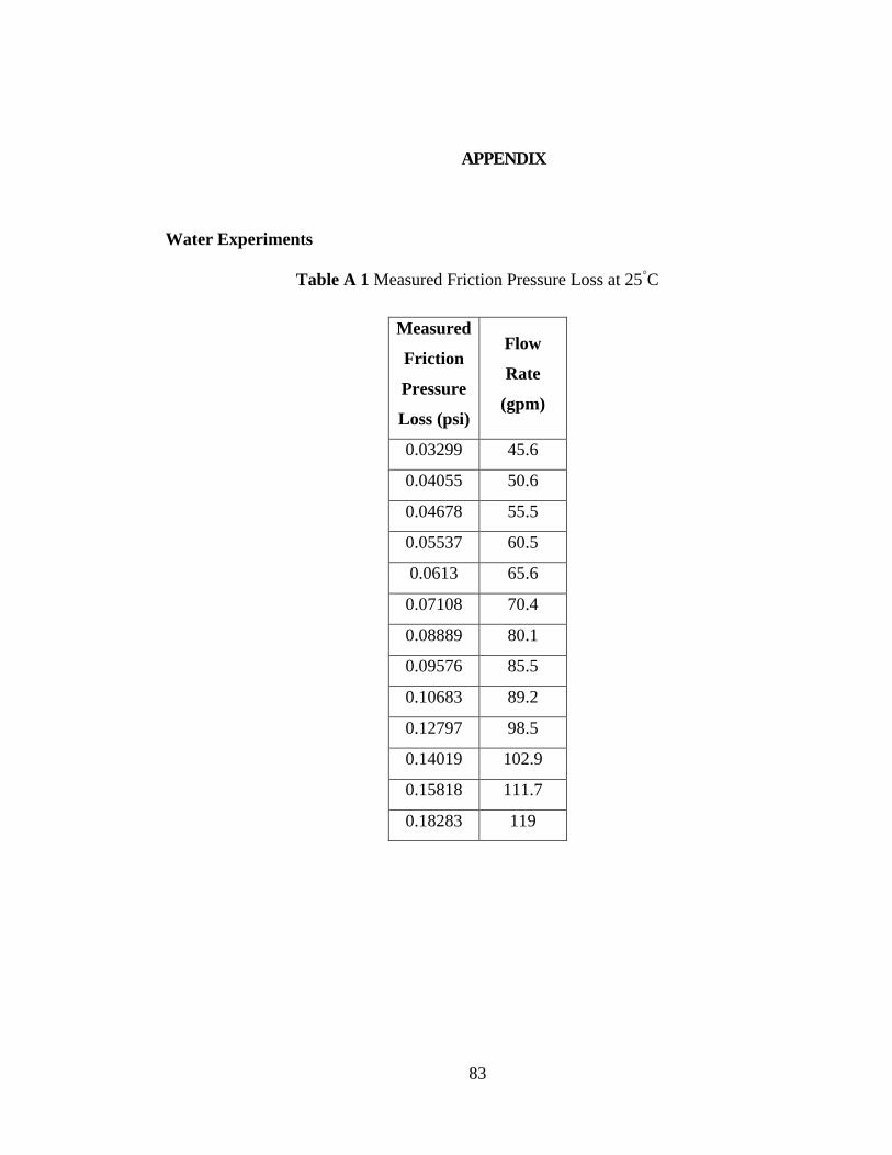
83

APPENDIX

Water Experiments

Table A 1 Measured Friction Pressure Loss at 25°C

Measured

Friction

Pressure

Loss (psi)

Flow

Rate

(gpm)

0.03299 45.6

0.04055 50.6

0.04678 55.5

0.05537 60.5

0.0613 65.6

0.07108 70.4

0.08889 80.1

0.09576 85.5

0.10683 89.2

0.12797 98.5

0.14019 102.9

0.15818 111.7

0.18283 119

84

Table A 2 Measured Friction Pressure Loss at 35°C

Measured

Friction

Pressure

Loss (psi)

Flow

Rate

(gpm)

0.02253 40.4

0.03084 45.4

0.03658 50.5

0.04521 55.3

0.04964 60.6

0.05982 65.6

0.06423 69.1

0.07748 75.1

0.08897 82.2

0.11151 93.3

0.12325 99.1

0.13968 107.6

0.16314 112.6

85

Table A 3 Measured Friction Pressure Loss at 45°C

Measured

Friction

Pressure

Loss (psi)

Flow

Rate

(gpm)

0.02839 45.4

0.03669 50.5

0.04049 55.1

0.04794 60.3

0.05644 65.6

0.0629 70.5

0.07237 75.7

0.08064 80.8

0.0923 85.8

0.09813 90.4

0.10895 95.4

0.11159 96.5

0.12051 101.7

0.13249 106.8

0.14333 110.7

86

Polymeric Drilling Fluid Experiments

Table A 4 Measured Friction Pressure Loss at 30°C

Measured

Friction

Pressure

Loss (psi)

Flow

Rate

(gpm)

0.04065 26.6

0.04395 30.5

0.04864 35.5

0.06262 45.6

0.07555 55.6

0.081 60.1

0.08462 65.5

0.0957 75.3

0.10708 85.2

0.11656 95.5

0.13908 105.8

0.16263 113.43

87

Table A 5 Measured Friction Pressure Loss at 37°C

Measured

Friction

Pressure

Loss (psi)

Flow

Rate

(gpm)

0.0361 30.4

0.03892 35.5

0.05081 40.5

0.05763 45.4

0.06667 55.5

0.07078 60.5

0.07686 66.3

0.08438 75.6

0.08888 80.5

0.09658 85.6

0.13288 99.4

0.16593 110.8

88

Table A 6 Measured Friction Pressure Loss at 44°C

Measured

Friction

Pressure

Loss (psi)

Flow

Rate

(gpm)

0.02918 30.4

0.03273 35.5

0.035 39.5

0.04542 50.5

0.05435 55.6

0.0714 64.5

0.07215 70

0.0896 83.4

0.105 91.5

0.12187 100.4

0.16347 114.1