Copyright © 2014, 2015 by William Schmidt and Ryan W. Buell

Working papers are in draft form. This working paper is distributed for purposes of comment and discussion only. It may not be reproduced without permission of the copyright holder. Copies of working papers are available from the author.

Experimental Evidence of Pooling Outcomes Under Information Asymmetry William Schmidt Ryan W. Buell

Working Paper

15-001 October 21, 2015

Experimental Evidence of Pooling Outcomes Under Information

Asymmetry

William Schmidt∗, Ryan W. Buell†

October 21, 2015

Abstract

Operational decisions under information asymmetry can signal a firm’s prospects to less-

informed parties, such as investors, customers, competitors, and regulators. Consequently, man-

agers in these settings often face a tradeoff between making an optimal decision and sending a

favorable signal. We provide experimental evidence on the choices made by decision makers in

such settings. Equilibrium assumptions that are commonly applied to analyze these situations

yield the least cost separating outcome as the unique equilibrium. In this equilibrium, the more

informed party undertakes a costly signal to resolve the information asymmetry that exists. We

provide evidence, however, that participants are much more likely to pursue a pooling outcome

when such an outcome is available. This result is important for research and practice because

pooling and separating outcomes can yield dramatically different results and have divergent

implications. We find evidence that the choice to pool is influenced by changes in the underly-

ing newsvendor model parameters in our setting. In robustness tests, we show that choosing a

pooling outcome is especially pronounced among participants who report a high level of under-

standing of the setting and that participants who pool are rewarded by the less informed party

with higher payoffs. Finally, we demonstrate through a reexamination of Lai et al. (2012) and

Cachon and Lariviere (2001) how pooling outcomes can substantively extend the implications

of other extant signaling game models in the operations management literature.

∗The Johnson School, Cornell University, Sage Hall, Ithaca NY 14853. E-mail: wschmidt@cornell.edu.†Harvard Business School, Soldiers Field Park, Boston MA 02163. E-mail: rbuell@hbs.edu.

1 Introduction

Operational decisions under information asymmetry can signal a firm’s prospects to less-informed

parties, such as investors, customers, competitors, and regulators. Consequently, managers in

these settings often face a tradeoff between making an optimal decision and sending a favorable

signal.1 These decisions and their implications are well-examined using signaling game models in

the operations literature, but there is limited empirical evidence to validate the predictions of these

models. We address this gap by testing the predictive power of equilibrium assumptions in signaling

games with information asymmetry among the participants.

Signaling game theory has been used to study the implications of information asymmetry in

a wide array of decision contexts, including consumer purchases (Debo and Veeraraghavan 2010),

competitive entry (Anand and Goyal 2009), new product introductions (Lariviere and Padmanab-

han 1997), franchising (Desai and Srinivasan 1995), channel stuffing (Lai et al. 2011), supply chain

coordination (Cachon and Lariviere 2001, Ozer and Wei 2006, Islegen and Plambeck 2007), and

capacity investments (Lai et al. 2012, Schmidt et al. 2015). In these works, researchers must decide

how to address the multiple equilibria outcomes that invariably arise. Often the emphasis is on the

least cost separating outcome in which the informed party over-invests in a costly signal in order

to credibly reveal her private information to the less informed party.

The alternative class of equilibria is a pooling outcome, in which the informed party either over-

invests or under-invests, depending on its private information. Researchers often exclude pooling

outcomes from consideration either for convenience or by invoking equilibrium assumptions that,

although commonly applied, have not been empirically validated. In the first instance, Cachon and

Lariviere (2001), Ozer and Wei (2006) and Islegen and Plambeck (2007) acknowledge that pooling

equilibria exist, but opt to focus their analyses on the least cost separating outcome as they are

particularly interested in examining situations in which the more informed player can credibly reveal

her type. In the second instance, Desai and Srinivasan (1995), Lariviere and Padmanabhan (1997)

1Managers may engage in such myopic decision making for a variety of reasons, including career advancement

(Narayanan 1985, Holmstrom 1999) or secondary equity raises (Stein 2003). Barton (2011) uses the term “quarterly

capitalism” to decry a common situation in which firms are induced to make decisions based on short-term market

pressures. This issue is salient to operations management because managers generally prefer manipulating operational

decisions over accounting manipulations to meet performance benchmarks (Bruns and Merchant 1990, Graham et al.

2005).

1

and Lai et al. (2012) make equilibrium assumptions by employing the Intuitive Criterion refinement

(described in Section 2.1) to eliminate all possible pooling equilibria such that only the least cost

separating equilibrium remains. More elaborate signaling games, such as those with more than one

signaling mechanism (Debo and Veeraraghavan 2010), limited signaling capacity (Lai et al. 2011),

or more than two players (Anand and Goyal 2009), also employ the Intuitive Criterion refinement,

although the refinement may not generate a unique equilibrium prediction in these cases. Missing

from this research is a consideration of alternative equilibrium assumptions, which yield different

predicted outcomes and insights when applied to these models.

To shed light on this issue, we conduct a controlled experiment to examine whether separating or

pooling outcomes more accurately describe actual decision making. Our work differs from literature

that tests the validity of behavioral assumptions in models of managerial decision making. Such

studies examine the behavioral factors that may influence personal choices. For instance, several

behavioral experimental studies have identified that decision makers may deviate from the expected-

profit-maximizing capacity choice due to decision biases, including anchoring, demand chasing, and

inventory error minimization (Schweitzer and Cachon 2000, Bolton and Katok 2008, Bostian et al.

2008, Kremer et al. 2010). We contribute to this line of investigation by testing the predictive

power of equilibrium assumptions in models of managerial decision making. In doing so, our

research identifies a novel explanation of managerial deviations from model predictions in practical

settings.

Our experimental design, detailed in Section 3.1, is most closely related to the capacity in-

vestment models in Bebchuk and Stole (1993), Lai et al. (2012) and Schmidt et al. (2015). Our

results strongly support that decision makers adopt pooling outcomes rather than least cost sepa-

rating outcomes when (1) both pooling and separating outcomes exist and (2) commonly accepted

equilibrium assumptions would otherwise predict separating outcomes.

To motivate our experiment, we expand the model in Lai et al. (2012) to include consideration

of pooling alternatives. We show that when pooling exists it produces higher expected payoffs for

the informed party than the least cost separating outcome. These results demonstrate the intuition

behind the experimental evidence supporting pooling outcomes – namely that pooling outcomes can

yield higher payoffs than separating outcomes. The results also align with our finding (described

in Section 5.3) that participants who make pooling decisions earn higher payoffs than those who

2

decide to separate.

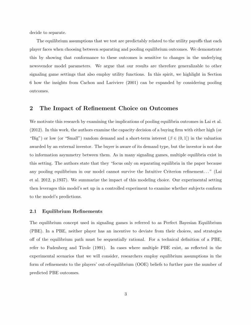
The equilibrium assumptions that we test are predictably related to the utility payoffs that each

player faces when choosing between separating and pooling equilibrium outcomes. We demonstrate

this by showing that conformance to these outcomes is sensitive to changes in the underlying

newsvendor model parameters. We argue that our results are therefore generalizable to other

signaling game settings that also employ utility functions. In this spirit, we highlight in Section

6 how the insights from Cachon and Lariviere (2001) can be expanded by considering pooling

outcomes.

2 The Impact of Refinement Choice on Outcomes

We motivate this research by examining the implications of pooling equilibria outcomes in Lai et al.

(2012). In this work, the authors examine the capacity decision of a buying firm with either high (or

“Big”) or low (or “Small”) random demand and a short-term interest (β ∈ (0, 1]) in the valuation

awarded by an external investor. The buyer is aware of its demand type, but the investor is not due

to information asymmetry between them. As in many signaling games, multiple equilibria exist in

this setting. The authors state that they “focus only on separating equilibria in the paper because

any pooling equilibrium in our model cannot survive the Intuitive Criterion refinement. . . ” (Lai

et al. 2012, p.1937). We summarize the impact of this modeling choice. Our experimental setting

then leverages this model’s set up in a controlled experiment to examine whether subjects conform

to the model’s predictions.

2.1 Equilibrium Refinements

The equilibrium concept used in signaling games is referred to as Perfect Bayesian Equilibrium

(PBE). In a PBE, neither player has an incentive to deviate from their choices, and strategies

off of the equilibrium path must be sequentially rational. For a technical definition of a PBE,

refer to Fudenberg and Tirole (1991). In cases where multiple PBE exist, as reflected in the

experimental scenarios that we will consider, researchers employ equilibrium assumptions in the

form of refinements to the players’ out-of-equilibrium (OOE) beliefs to further pare the number of

predicted PBE outcomes.

3

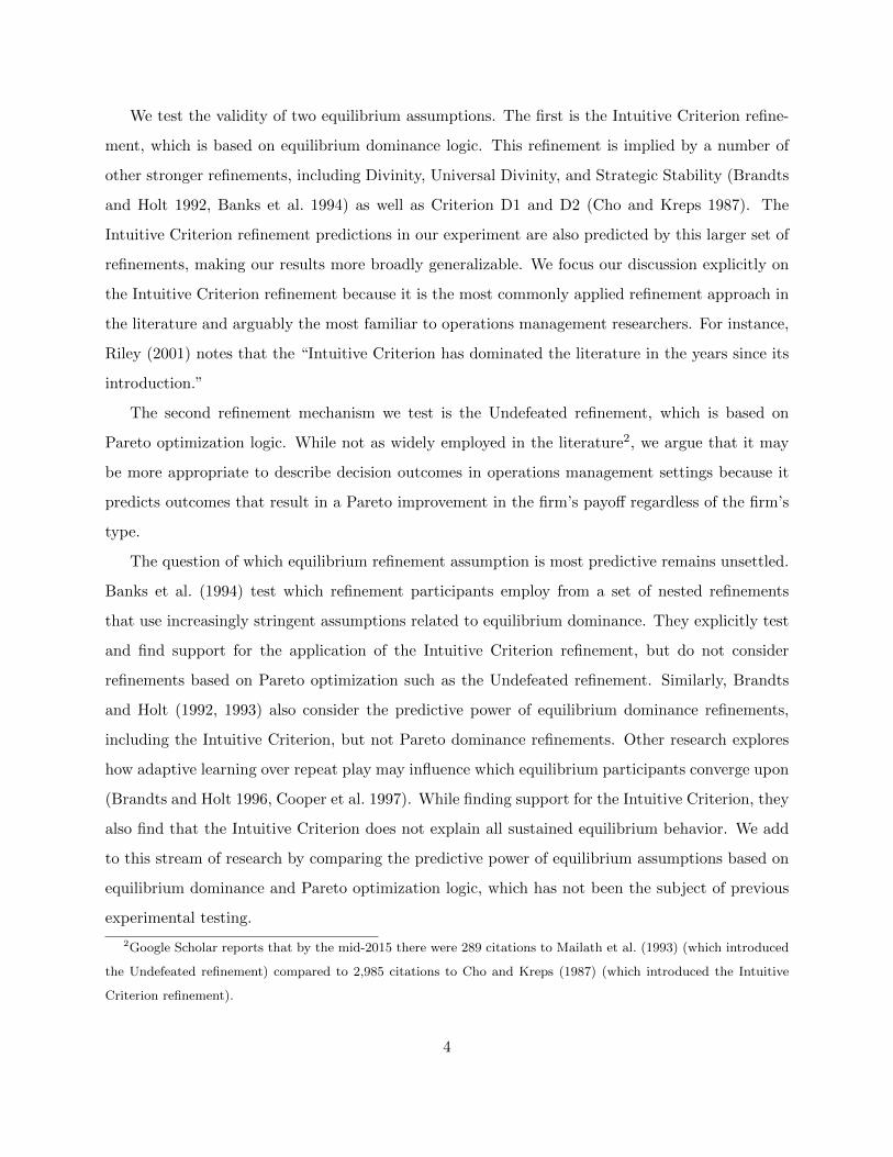
We test the validity of two equilibrium assumptions. The first is the Intuitive Criterion refine-

ment, which is based on equilibrium dominance logic. This refinement is implied by a number of

other stronger refinements, including Divinity, Universal Divinity, and Strategic Stability (Brandts

and Holt 1992, Banks et al. 1994) as well as Criterion D1 and D2 (Cho and Kreps 1987). The

Intuitive Criterion refinement predictions in our experiment are also predicted by this larger set of

refinements, making our results more broadly generalizable. We focus our discussion explicitly on

the Intuitive Criterion refinement because it is the most commonly applied refinement approach in

the literature and arguably the most familiar to operations management researchers. For instance,

Riley (2001) notes that the “Intuitive Criterion has dominated the literature in the years since its

introduction.”

The second refinement mechanism we test is the Undefeated refinement, which is based on

Pareto optimization logic. While not as widely employed in the literature2, we argue that it may

be more appropriate to describe decision outcomes in operations management settings because it

predicts outcomes that result in a Pareto improvement in the firm’s payoff regardless of the firm’s

type.

The question of which equilibrium refinement assumption is most predictive remains unsettled.

Banks et al. (1994) test which refinement participants employ from a set of nested refinements

that use increasingly stringent assumptions related to equilibrium dominance. They explicitly test

and find support for the application of the Intuitive Criterion refinement, but do not consider

refinements based on Pareto optimization such as the Undefeated refinement. Similarly, Brandts

and Holt (1992, 1993) also consider the predictive power of equilibrium dominance refinements,

including the Intuitive Criterion, but not Pareto dominance refinements. Other research explores

how adaptive learning over repeat play may influence which equilibrium participants converge upon

(Brandts and Holt 1996, Cooper et al. 1997). While finding support for the Intuitive Criterion, they

also find that the Intuitive Criterion does not explain all sustained equilibrium behavior. We add

to this stream of research by comparing the predictive power of equilibrium assumptions based on

equilibrium dominance and Pareto optimization logic, which has not been the subject of previous

experimental testing.

2Google Scholar reports that by the mid-2015 there were 289 citations to Mailath et al. (1993) (which introduced

the Undefeated refinement) compared to 2,985 citations to Cho and Kreps (1987) (which introduced the Intuitive

Criterion refinement).

4

2.1.1 The Intuitive Criterion Refinement

In our context, the Intuitive Criterion refinement is applied by considering all possible OOE capacity

levels for a particular PBE and identifying whether, compared to the PBE results, a capacity choice

exists that would not provide a “Small” demand firm with a higher payoff using the highest valuation

the investor could assign but would provide a “Big” demand firm with a higher payoff using the

highest valuation the investor could assign. If such a capacity choice does exist then the Intuitive

Criterion refinement eliminates the focal PBE. In signaling games involving two players, one costly

signal with continuous and infinite support, two types of the informed player, and conformance

with the single crossing property, the Intuitive Criterion eliminates all but the least cost separating

PBE. For the formal definition of the Intuitive Criterion refinement, please refer to Cho and Kreps

(1987).

Although it is widely applied in the literature, there are practical concerns with the Intuitive

Criterion that may make it inappropriate in some operations management settings. For instance,

the Intuitive Criterion refinement (1) asserts that decision makers will make choices that involve

costly signaling even if such choices are Pareto-dominated by alternative choices (Mailath et al.

1993), (2) assumes that counterfactual information can be communicated in the game without

being explicitly modeled (Salanie 2005), (3) may eliminate all choices from consideration when

signals have discrete support (Schmidt et al. 2015), and (4) can lead to implausible outcomes

(Bolton and Dewatripont 2005).

2.1.2 The Undefeated Refinement

The Undefeated refinement is based on Pareto-optimization logic. If there exists multiple PBE in a

game, and one of those PBE provides a Pareto improvement in payoffs for all types of the informed

player compared to one of the alternative PBE, then the Pareto dominated PBE is eliminated.

A PBE which is not Pareto dominated by any alternative PBE is said to be “undefeated” or to

survive the Undefeated refinement. As a result, the Undefeated refinement predicts the outcome

which yields the highest equilibrium payoff for each type of informed player. In some cases this

may be a separating PBE and in other cases this may be a pooling PBE. For a technical definition

of the Undefeated refinement, please refer to Mailath et al. (1993). In some cases there may exist

multiple pooling PBE that survive the Undefeated refinement. For ease of exposition in our analysis

5

of Lai et al. (2012) and Cachon and Lariviere (2001), we focus on the unique pooling PBE that is

a lexicographically maximum sequential equilibrium (LMSE). According to Mailath et al. (1993),

a PBE is a LMSE if among all PBE it maximizes the utility for a high type, and conditional on

maximizing the utility for a high type, it then maximizes the utility for a low type. Using a LMSE

to identify a unique PBE is intuitively appealing because typically a low type wishes to be perceived

as a high type rather than the opposite.

Although not widely adopted, the Undefeated refinement has been applied in the finance and

economics literature (Spiegel and Spulber 1997, Taylor 1999, Gomes 2000, Fishman and Hagerty

2003) and it addresses the concerns highlighted in Section 2.1.1 about the Intuitive Criterion re-

finement. An intuitive result of the Undefeated refinement is that when one or more pooling PBE

exist, then one pooling PBE which will survive the Undefeated refinement is an outcome in which

every type of the informed player mimics the optimal pooling choice of the highest type.3

2.2 An Example of the Impact of Refinement Choice

We replicate the example from Section 4 of Lai et al. (2012) using the Intuitive Criterion refinement

and compare the results to those obtained if the Undefeated refinement is used instead. In this

example, the buying firm faces a newsvendor profit function with a selling price (p) of 20, a wholesale

price (w) of 8, and a buyback price (b) of 4. The supplier has a production cost (c) of 5. The

prior probability that the buyer’s demand signal is high (λ) is 0.5 and demand follows a gamma

distribution with a scale parameter of 5 for both buyer types, a shape parameter of 1.5 for buyer

types facing a high demand, and a shape parameter of 1.0 for buyer types facing a low demand.

The buyer chooses a stocking level q, which may signal its type to the uniformed party. Refer to

Lai et al. (2012) for further details.

There are a range of model parameters over which a separating equilibrium exists and a sub-

3This can be valid even as the game structure gets complex. For instance, under infinite types, infinite strategies,

and infinite state spaces, a more rigorous application for a given state space is the following program: (1) the highest

firm type identifies her optimal capacity choice provided the investors’ beliefs are unchanged (i.e. posterior beliefs =

prior beliefs), (2) the highest type compares her utility at that capacity level with her utility from separating, and

(3) if the highest type receives a higher utility under the capacity level from (1), then all firm types should choose

the capacity level from (1) provided it generates a higher utility for them compared to separating. Step (1) can be

done easily by, for instance, solving a newsvendor model in the case of stochastic demand. Steps (2) and (3) can be

done by solving the utility function for each firm type at the two alternative capacity choices.

6

stantial subset of this range over which both separating and pooling equilibria exist. Figure 1a,

corresponding to Figure 2 in Lai et al. (2012), utilizes the setup described above and β = 0.4 to

exemplify an instance in which only a separating equilibrium exists. In the separating equilibrium

the low type chooses q∗L and the high type chooses q. Figure 1b, utilizes the same setup and β

= 0.7 to exemplify an instance in which both a pooling and a separating equilibrium exist. In

the pooling equilibrium, both buyer types choose capacity qp while in the separating equilibrium

the low type chooses q∗L and the high type chooses q (note that q in Figure 1b is larger than in

Figure 1a, reflecting the higher cost of separating as β increases). Figure 1b makes clear the benefit

accrued to the buyer by pooling. In the pooling outcome, the high type buyer receives a utility

of 61.7 (labeled point C), which is 4% higher than the utility of 59.5 from the separating outcome

(point D). The low type buyer receives a utility of 53.7 in the pooling outcome (point A), which is

12% higher than the utility of 47.8 from the separating outcome (point B).

The intuition for why an increase in short term-ism leads to a pooling equilibrium under the

Undefeated refinement is clear in Figures 1b and 1a. Such an increase gives the low type buyer

a greater incentive to secure a higher short-term valuation by mimicking the high type buyer’s

stocking level. This increases the cost of separating for the high type, which in turn makes a

pooling outcome more attractive relative to separating for the high type. Schmidt et al. (2015)

show rigorously that other model parameters, including a decrease in the prior belief that the firm

is a low type and changes in the newsvendor model parameters, can increase the likelihood that a

pooling equilibrium exists.

Expanding on this example, Lai et al. (2012) show that buyers must send a costly signal in

order to separate when β > β, where β ≈ 0.21. It can be shown that a pooling equilibrium also

exists when β > β, where β ≈ 0.60.4 As shown in Figure 2a, the pooling equilibrium provides a

materially higher expected utility for the buyer compared to the separating equilibrium. In fact, the

pooling equilibrium becomes an increasingly attractive alternative to the separating equilibrium as

β increases and the cost of separating drags down the buyer’s expected utility under the separating

equilibrium. The discontinuity in Figure 2a at β = 0.60 can be understood by examining Figure 2b.

This figure shows the percent improvement of the pooling equilibrium compared to the separating

equilibrium for each buyer type and in expectation. At the threshold value of β = 0.60, the high

4Different model parameters will result in different threshold values for β and β.

7

Figure 1: Buyer’s Profit as a Function of Capacity.

(a) Excluding a pooling equilibrium (β = 0.40).

0

10

20

30

40

50

60

70

80

0 5 10 15 20

Bu

yer

's e

xpec

ted

Pay

off

q

Low type, high valuation High type, high valuation

Low type, low valuation High type, low valuation

q*L

GH(q)

GL(q)

GLH(q)

GHL(q)

q*HL

qq

(b) Including a pooling equilibrium (β = 0.70).

0

10

20

30

40

50

60

70

80

0 5 10 15 20

Buyer

's e

xpec

ted P

ayoff

q

Low type, high valuation High type, high valuation

Low type, weighted valuation High type, weighted valuation

Low type, low valuation High type, low valuation

D

B

A

C

q*L

GH(q)

GL(q)

GLH(q)

GHL(q)

q*HL qp qq

GHW(q)

GLW(q)

type buyer is ambivalent between pooling and separating, while the low type buyer strictly prefers

to pool. Above this threshold, both types benefit from pooling, leading to the existence of a pooling

equilibrium.

Note that the objective of our analysis is to identify participant choices when both separating

and pooling equilibria exist (β > β in this example). When only the separating equilibria exists

(β < β) the equilibrium assumptions tested in our experiment yield identical predictions.

3 Model and Scenario Development

3.1 Player Payoffs

The payoffs in our experiment are theoretically grounded by models employed in Bebchuk and Stole

(1993), Lai et al. (2012) and Schmidt et al. (2015). We apply the following set up in Section 3.2 to

develop scenarios for the experiment. There are two players, the firm (denoted F ) and an investor

in the firm (denoted I). The firm can be one of two types with respect to its market prospects – a

“Small” opportunity type (τS) or a “Big” opportunity type (τB). The probability that a firm will

be type τS is denoted (1 − λ) and type τB is denoted λ, where λ ∈ (0, 1). The firm types differ

only in the probability distribution of demand. The demand distribution for a τB type first order

stochastically dominates (FOSD) the demand distribution for a τS type, i.e., FS(x) ≥ FB(x) for

8

Figure 2: Buyer’s Expected Utility and Surplus Benefit from a Pooling Equilibrium

(a) Buyer’s Expected Utility Under Pooling and Sep-

arating Equilibria

0 0.2 0.4 0.6 0.8 145

50

55

60

65

Buy

er’s

Exp

ecte

d U

tility

β

Pooling PBESeparating PBE

ββ

(b) Percent Improvement for Each Buyer Type from

a Pooling Equilibrium Compared to a Separating

Equilibrium

0 0.2 0.4 0.6 0.8 10

5

10

15

20

25

Perc

enta

ge o

f su

rplu

s in

crem

ent

β

ExpectationHigh typeLow type

all x ∈ <+ and FS(x) > FB(x) for some x, where Fτ (·) is the cumulative distribution function

of demand for type τ . The assumptions reflected in our experiment5 are commonly used in the

signaling game literature (Kreps and Sobel 1992).

The firm must decide how many stores to open (q), where q can be in multiples of a capacity

increment Q, i.e., q = nQ for some integer n.6 The firm’s payoff is a linear combination of the

investor’s valuation of the firm (ρ(q)) and the firm’s expected profit (π(τ, q)), weighted by β and

1− β respectively, where β ∈ (0, 1]:

U(τ, q, ρ) = βρ(q) + (1− β)π(τ, q). (1)

A larger value of β corresponds to a higher emphasis on short-term valuation and a correspondingly

lower emphasis on the expected long-term expected profits. The firm’s expected profit is derived

5Two players, one costly signal, two types of the informed player, and the single crossing property holds.6Using discrete choices simplifies the experience for the subject and is consistent with findings in the experimental

literature that limiting the choice set is a valid de-biasing strategy (Bolton and Katok 2008).

9

by solving the newsvendor model, π(τ, q) = Eτ [pmin{q, x}+ w(q − x)+ − bq] where p is the selling

price, w is the wholesale cost, and b is the buyback price of unsold inventory; p > w > b. Note that

if β = 0 then Equation 1 resolves to the classical newsvendor model.

Upon seeing the number of stores q that the firm decides to open, the investor must decide

what valuation ρ(q) to assign to the firm. The investor can assign three values to the firm – “Big”

(which corresponds to ρ(q) = π(τB, q)), “Weighted” (which corresponds to ρ(q) = (1−λ)π(τS , q) +

λπ(τB, q)), or “Small” (which corresponds to ρ(q) = π(τS , q)). The investor’s payoff depends on

being as close as possible to the true value of the firm:

V (τ, q, ρ) = −[π(τ, q)− ρ(q)]2.

3.2 Scenario Development

Following the model described in Section 3.1, we developed a set of 4,752 scenarios for potential

inclusion in the experiment. These scenarios were generated using a manageable subset of the

parameters utilized in Schmidt et al. (2015). Specifically, the firm faces a log-normal demand

distribution regardless of its type with a log-scale parameter for a τS type of µS = 6.0 and for a τB

type of µB ∈ {6.25, 6.50}. The shape parameter takes values σ2 ∈ {0.15, 0.25}. The unit price (p)

ranges from 0.75 to 1.00 in increments of 0.05, unit buyback price / salvage value (b) ranges from

0.0 to 0.10 in increments of 0.05, and unit wholesale price is w = 0.4. Short-termism (β) ranges

from 0.10 to 0.60 in increments of 0.05, the equity holder’s prior beliefs that the firm is type τS

(1−λ) ranges from 0.30 to 0.40 in increments of 0.05, and the capacity investment is discrete with

Q ∈ {100, 200}.

We then identified three scenarios from this set of 4,752 scenarios, and manually confirmed that

each selected scenario satisfies two conditions. First, the scenario must simultaneously test the

predictive power of the Undefeated and Intuitive Criterion refinements. To achieve this, we used

scenarios with four sequential capacity values based on the capacity increment Q. The first capacity

value must optimize the payoff for a τS type when receiving a low valuation, survive the Intuitive

Criterion refinement, and be eliminated by the Undefeated refinement. The second capacity value

must optimize the payoff for a τB type when receiving a weighted valuation, survive the Undefeated

refinement, and be eliminated by the Intuitive Criterion refinement. The third capacity value must

not be a PBE (it is necessary for inclusion due to its role in the application of the Intuitive Criterion

10

refinement). The fourth capacity value must be the least-cost separating capacity for a τB type,

survive the Intuitive Criterion refinement, and be eliminated by the Undefeated refinement.

The second condition for a scenario’s inclusion is that if the unit price used in the scenario is

incremented by 0.05 it yields a new scenario with four valid capacity values. This condition allowed

us to test the impact on participant choices of changing the unit price in the newsvendor model.

If a scenario did not meet both conditions, another scenario from the pool of 4,752 scenarios was

selected and manually evaluated. This process was repeated until three scenarios meeting both

conditions were identified. By incrementing the price by 0.05 in each of these three scenarios,

three additional scenarios were generated, for a total of six scenarios in the experiment. Table

1 summarizes the model parameters used to generate each of the six scenarios included in the

experiment.

To more realistically reflect the store opening choice that is the basis of the firm’s decision in the

experiment, we divided the capacity options by 100 in the scenarios. We applied a positive linear

transformation to the payoffs in each scenario so that the range of possible payments fit our budget

limitations. Positive linear transformations are commonly used to represent the same preferences as

the original payoff function while preserving the expected utility property (Mas-Colell et al. 1995).

None of the choices in any scenario are strictly dominated, so there is no guarantee that any

particular choice will result in a player realizing a higher payoff. A choice is strictly dominated for

a firm type if the best utility that firm type could possibly achieve by sending that signal is strictly

lower than the worst utility that firm type could possibly achieve by sending some other signal.

For a technical definition of Strict Dominance, refer to (Mas-Colell et al. 1995, p.469).

Figure 3a provides the extensive form view of scenario 1, shown from the firm’s perspective.

The investor’s perspective was identical to that of the firm, except for minor coloration and prompt

differences, which served to highlight each player’s choice set and payoffs. In this scenario the firm

faced a “Big” opportunity with an ex-ante probability of 65%. A “Big” opportunity firm could

choose to open 5, 6 or 7 stores, while a “Small” opportunity firm could choose to open 4, 5, or

6 stores. If the firm chose to open a pooling quantity of either 5 or 6 stores, then the investor

was prompted to decide whether to award the firm a “Small,” “Weighted,” or “Big” valuation.

If instead, the firm chose a separating quantity of 4 or 7 stores, the investor was notified of the

quantity and informed that the firm is a “Small” or “Big” opportunity firm, respectively. The

11

players’ payoffs for each outcome are summarized near the terminal node for the outcome.

Figure 3: Extensive form of Scenarios 1 and 2.

(a) Extensive form of Scenario 1, shown from the

firm’s perspective. There is a 35% probability that

the participant in the role of the firm is randomly

assigned to be a “Small” opportunity type firm.

(b) Extensive form of Scenario 2, shown from the in-

vestor’s perspective. There is a 35% probability that

the participant in the role of the firm is randomly

assigned to be a “Small” opportunity type firm.

There are two PBE in Scenario 1, (1) the least cost separating PBE in which a “Big” type

chooses 7 stores and a “Small” type chooses 4 stores and (2) a pooling PBE in which both firm

types choose 5 stores. In the separating PBE, the “Big” type is guaranteed to earn $0.67 and the

“Small” type is guaranteed to earn $0.52. The investor earns $1.00 regardless of the firm’s type.

In the pooling PBE at 5 stores, the “Big” type earns $0.84 under a “Weighted” valuation and the

“Small” type earns $0.63 under a “Weighted” valuation. The investor earns $0.90 in expectation

by awarding a “Weighted” valuation (0.65× $0.95 + 0.35× $0.82). Opening 6 stores is not a PBE.

It is not a separating PBE since a “Big” type cannot separate from a “Small” type by opening 6

stores, nor is it a pooling PBE since the “Small” type receives a higher payoff by opening 4 stores

than she does by opening 6 stores and receiving a “Weighted” valuation.

The separating PBE in each scenario survives the Intuitive Criterion refinement. The pooling

PBE at 5 stores does not survive the Intuitive Criterion refinement because there exists an alterna-

tive choice (opening 6 stores), which (1) provides the “Small” opportunity firm with a lower payoff

under a “Big” valuation compared to the payoff she receives under a “Weighted” valuation when

12

opening 5 stores and (2) provides the “Big” opportunity firm with a higher payoff under a “Big”

valuation compared to the payoff she receives under a “Weighted” valuation when opening 5 stores.

In other words, the best payoff that a “Small” firm can get by opening 6 stores ($0.59) is less than

the payoff they receive under a “Weighted” valuation when opening 5 stores ($0.63), and the best

payoff that a “Big” firm can get by opening 6 stores ($0.89) is greater than the payoff they receive

under a “Weighted” valuation when opening 5 stores ($0.84).

The separating PBE does not survive the Undefeated refinement since there exists an alter-

native PBE (pooling on 5 stores) which provides a higher equilibrium payoff for both firm types.

Specifically, the “Small” type receives a payoff of $0.63 under a “Weighted” valuation when open-

ing 5 stores compared to a payoff of $0.52 by opening 4 stores in the separating PBE. The “Big”

type receives a payoff of $0.84 under a “Weighted” valuation when opening 5 stores compared to

a payoff of $0.67 by opening 7 stores in the separating PBE. The pooling PBE at 5 stores survives

the Undefeated refinement since there does not exist an alternative PBE which provides a higher

equilibrium payoff for both firm types.

Figure 3b provides the extensive form view of Scenario 2 from the investor’s perspective. Note

that the structure of this scenario is similar to that of Scenario 1, although with different payoffs. In

this case, the payoffs are determined by increasing the unit price by 6.67% (from 0.75 to 0.80) in the

underlying newsvendor model used to generate the player payoffs. Figures 5 and 6 in the Appendix

provide the extensive forms for the remaining 4 scenarios. Scenario 4 is similar to Scenario 3

except that the unit price is increased by 6.67% (from 0.75 to 0.80) in the underlying newsvendor

model. Scenario 6 is similar to Scenario 5 except that the unit price is increased by 5.88% (from

0.85 to 0.90) in the underlying newsvendor model. This design facilitates our analysis by enabling

us to examine whether participants acted consistently across scenario pairs, as well as whether

participants’ choices were sensitive to changes in the underlying Newsvendor parameters. Table

2 identifies the outcomes predicted by the Undefeated and Intuitive Criterion refinements in each

experimental scenario.

4 Experiment

Participants. Participants (N=228, median age=25, 48% female) completed this experiment in a

laboratory at a university on the American East Coast in exchange for $15.00 plus an average bonus

13

of $10.37, which was based on the outcomes of the experimental games in which they participated.

The participants belonged to a subject pool associated with the university’s business school, and

registered for the study in response to an online posting. Roughly two-thirds of the participants were

full-time undergraduate or graduate students hailing from a wide array of fields. The remaining

participants were residents who lived in the surrounding community. Table 3 summarizes the

participant demographic information.

Experimental design and procedure. At the beginning of the session, a monitor read

a script aloud to familiarize the participants with their roles and the experimental procedure.

The text of the script is provided in the Online Appendix, and the accompanying presentation

slides are available from the authors upon request. Throughout the session, participants engaged

with one another anonymously, through a web-based software application that was developed for

this experiment. The software restricted communication between participants explicitly to the

decisions described below. Participants were not permitted to engage with one another outside of

the software.

Participants considered each of the six scenarios from the perspectives of both a firm and an

investor, resulting in a total of 12 rounds. At the beginning of each round, participants were

randomly and anonymously paired with one another and notified of their role for the round (firm

or investor). Next, the matched pair of participants was presented with the extensive form view of a

randomly selected scenario and the probability the firm faced a “Big” opportunity. Upon seeing the

extensive form representation, participants were asked to anticipate the choices they would make

under different realizations of the scenario. Participants playing the role of the firm were asked

how many stores they would open if they faced a “Big” or “Small” opportunity. The quantity

choices available to the firm represented different combinations of separating PBE, pooling PBE,

and choices that were not PBE. Concurrently, participants playing the role of the investor were

asked whether they would award a “Big,” “Weighted,” or “Small” valuation to the firm, if they

observed the firm select each of the pooling quantities under its consideration.

We elicited strategies from participants prior to capturing their direct responses during actual

game play for two reasons. First, by asking the participants to predefine their strategies, we hoped

to encourage them to consider each scenario from different perspectives before committing to a

final decision. Second, by engaging in this staged approach, we were able to control for whether

14

firms and investors deviated from their original strategies once information had been revealed to

them.7

Next, based on the stated probability, the software randomly designated the firm to be facing

a “Big” or “Small” opportunity, revealing this information only to the participant playing the role

of the firm. Upon receiving this private information, the participant playing the role of the firm

could confirm or revise the number of stores she chose to open. Then, the number of stores opened

by the firm (but not its type) was revealed to the investor, who could in turn, confirm or revise her

valuation.

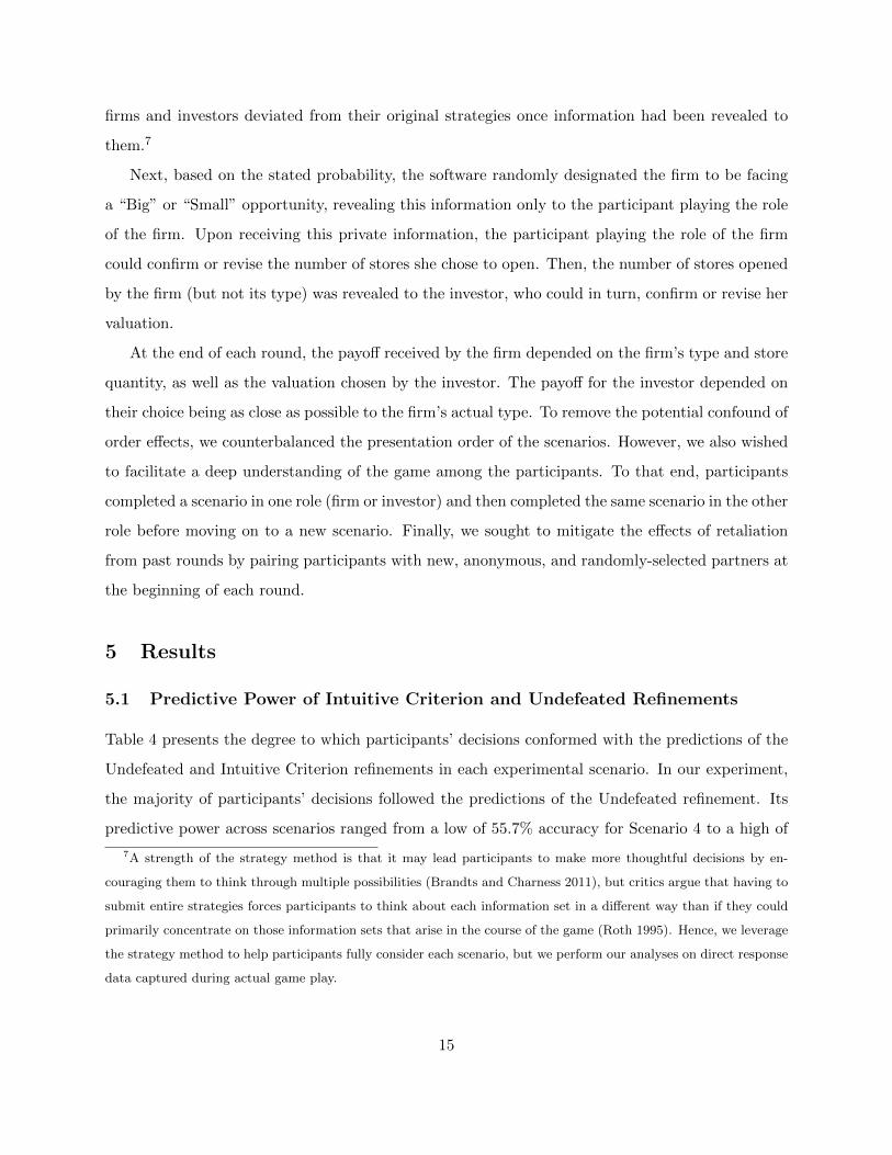
At the end of each round, the payoff received by the firm depended on the firm’s type and store

quantity, as well as the valuation chosen by the investor. The payoff for the investor depended on

their choice being as close as possible to the firm’s actual type. To remove the potential confound of

order effects, we counterbalanced the presentation order of the scenarios. However, we also wished

to facilitate a deep understanding of the game among the participants. To that end, participants

completed a scenario in one role (firm or investor) and then completed the same scenario in the other

role before moving on to a new scenario. Finally, we sought to mitigate the effects of retaliation

from past rounds by pairing participants with new, anonymous, and randomly-selected partners at

the beginning of each round.

5 Results

5.1 Predictive Power of Intuitive Criterion and Undefeated Refinements

Table 4 presents the degree to which participants’ decisions conformed with the predictions of the

Undefeated and Intuitive Criterion refinements in each experimental scenario. In our experiment,

the majority of participants’ decisions followed the predictions of the Undefeated refinement. Its

predictive power across scenarios ranged from a low of 55.7% accuracy for Scenario 4 to a high of

7A strength of the strategy method is that it may lead participants to make more thoughtful decisions by en-

couraging them to think through multiple possibilities (Brandts and Charness 2011), but critics argue that having to

submit entire strategies forces participants to think about each information set in a different way than if they could

primarily concentrate on those information sets that arise in the course of the game (Roth 1995). Hence, we leverage

the strategy method to help participants fully consider each scenario, but we perform our analyses on direct response

data captured during actual game play.

15

71.1% accuracy for both Scenarios 1 and 5. Participants’ decisions matched the predictions of the

Intuitive Criterion on far fewer occasions. Its predictive power across scenarios ranged from a low

of 17.1% accuracy for Scenarios 1 and 3 to a high of 29.4% accuracy for Scenario 2. Subjects made

choices that conformed with neither refinement between 10.7% of the time (Scenario 2) and 19.7%

of the time (Scenario 3).

We test whether the predictive power of each refinement is statistically significant using two-

sided binomial tests of the null hypothesis that each refinement has no predictive power. If the

conformance of participants’ decisions to the predictions of each refinement were the product of

random chance, then we would expect to see decisions conform to the refinement predictions one

third of the time since each scenario has three choices. The tests evaluate the degree to which

choices deviate from these expectations. We evaluate the predictive power of each refinement

in each scenario individually and then in aggregate. Participants’ decisions conformed with the

predictions of the Undefeated refinement in all six scenarios (p <0.001 two-sided for each scenario).

Aggregating across all scenarios, we found support for the predictive power of the Undefeated

refinement, which predicted 63.5% of participants’ decisions (p < 0.001; two-sided), relative to an

expectation of 33.3% if it instead had no predictive power.8

In contrast, participants’ decisions were not predicted by the Intuitive Criterion refinement. In

five of the six scenarios, participants made choices which conformed with the Intuitive Criterion

refinement less often than what would be expected if participants were simply making random se-

lections (p <0.05 two-sided, for Scenario 4, and p <0.001 two-sided for Scenarios 1, 3, 5 and 6). The

sole exception is Scenario 2 in which 29.4% (p = 0.23; two-sided) of participant responses conformed

with the Intuitive Criterion refinement, which is statistically indistinguishable from an expectation

of 33.3%. Across all scenarios combined, we find support that the Intuitive Criterion refinement,

which predicted 20.9% of participants’ decisions (p <0.001 two-sided), has less predictive power

than an expectation of 33.3% if participant choices were purely random.9

8As a robustness test, we also considered just the first scenario seen by each participant. Since scenarios are

randomly assigned, different scenarios will be presented first to different participants. We find strong support for

the predictive power of the Undefeated refinement, which predicted 56.1% of participants’ decisions, relative to an

expectation of 33.3% (p <0.001; two-sided).9We again considered just the first scenario seen by each participant and find that firms made choices which

conformed with the Intuitive Criterion refinement 24.6% of the time, far less often than what would be expected if

participants were simply making random selections (p <0.01 two-sided).

16

To test which refinement is more predictive, we perform a two-sided binomial test of the null

hypothesis that there is no difference in the predictive power of the two refinements. We discard 212

out of 1,368 observations in which participants made decisions that were not predicted by either

refinement, leaving 1,156 observations.10 If neither refinement were predictive, then we would

expect to see participants splitting their decisions evenly between the options. However, 869 of

1,156 choices (75.2%) conformed with the Undefeated refinement, while the remaining 287 choices

(24.8%) conformed with the Intuitive Criterion refinement. Results of the binomial tests reject the

null hypothesis in favor of the alternative that the Undefeated refinement is more predictive than

the Intuitive Criterion refinement (p < 0.001; two-sided).

5.2 Sensitivity to Newsvendor Unit Price

As described in Section 3.2, Scenarios 1 and 2 are the same in all respects except the unit price

used to determine the players’ payoffs is 6.67% higher in Scenario 2. The unit price has also been

increased in Scenario 4 relative to Scenario 3 and in Scenario 6 relative to Scenario 5. We use

two-sided binomial tests to determine whether participant choices differ across these scenario pairs.

Rows 2 and 4 of Table 4 summarize these results.

As shown in Table 4, conformance with the Undefeated refinement is higher in Scenarios 1, 3,

and 5 than in Scenarios 2, 4 and 6. The difference in the proportion of participants whose choice

conforms with the Undefeated refinement between Scenarios 1 and 2 (diff = 0.114, p <0.05 two-

sided), Scenarios 3 and 4 (diff = 0.075, p =0.11 two-sided), and Scenarios 5 and 6 (diff = 0.105,

p <0.05 two-sided), are all positive and the first and third differences are statistically significant.

Comparing all odd scenarios to all even scenarios, the difference is positive and statistically sig-

nificant (diff = 0.098, p <0.001 two-sided). Conformance with the Intuitive Criterion refinement

is lower in Scenarios 1, 3, and 5 than in Scenarios 2, 4 and 6. The difference in the proportion

of participants whose choice conforms with the Intuitive Criterion refinement between Scenarios 1

and 2 (diff = -0.123, p <0.01 two-sided), Scenarios 3 and 4 (diff = -0.088, p <0.05 two-sided), and

Scenarios 5 and 6 (diff = -0.048, p =0.18 two-sided), are all negative and the first and second differ-

ences are statistically significant. Comparing all odd scenarios to all even scenarios, the difference

10We note that participants made choices that failed to conform with either refinement in 15.5% of cases (p <0.001

two-sided), which is significantly less frequent than random chance.

17

is negative and statistically significant (diff = -0.086, p <0.001 two-sided).

To understand these results, recall from Section 2.1 that the Undefeated refinement predicts

the outcome (either a separating PBE or a pooling PBE) which provides the highest equilibrium

payoff to both firm types. As the differential payoff between the PBE alternatives is reduced,

participants will become indifferent between them. In our scenarios, an increase in unit price

reduces the proportional improvement of the pooling PBE payoff relative to the separating PBE

payoff for “Big” opportunity firms while leaving the proportional payoffs largely unchanged for

the “Small” opportunity firms. For instance, in Scenario 1 the equilibrium payoff for the “Big”

opportunity firm that chooses a pooling PBE at 5 stores is 25% higher than the payoff received by

separating ($0.84 versus $0.67). The increase in unit price in Scenario 2 reduces this improvement

in the equilibrium payoff to 11% ($1.15 versus $1.04).11 The change in relative payoffs between

scenarios is much less pronounced for the “Small” opportunity firms, which receive a 21% higher

payoff in the pooling PBE in Scenario 1 ($0.63 versus $0.52) and a 19% higher payoff in Scenario

2 ($0.92 versus $0.77).12

Using this rationale, we expect to see a smaller proportion of “Big” opportunity firms com-

ply with the Undefeated refinement in Scenario 2 compared to Scenario 1, and approximately the

same proportion of “Small” opportunity firms. As summarized in Table 5, our results confirm this

intuition. The proportion of “Big” opportunity firms making choices that comply with the Unde-

feated refinement is 19.3 percentage points lower in Scenario 2 compared to Scenario 1 (p <0.001

two-sided) while the proportion of “Small” opportunity firms making choices that comply with the

Undefeated refinement is 0.9 percentage points lower in Scenario 2 compared to Scenario 1 (p =0.90

two-sided). Table 5 shows similar results comparing Scenario 3 to Scenario 4 and Scenario 5 to

Scenario 6.

These findings support the underlying logic behind the Undefeated refinement that firms make

choices based on the Pareto improvement in equilibrium outcomes. As the improvement in equilib-

rium payoffs between a pooling PBE and a separating PBE increases (diminishes), the pooling PBE

11The pattern of a material reduction in the proportional improvement in the “Big” opportunity firm’s payoffs

from the pooling PBE compared to the separating PBE is also present between Scenarios 3 (24% improvement) and

4 (12% improvement) and between Scenarios 5 (16% improvement) and 6 (6% improvement).12There is also a much more muted change in the proportional improvement in the “Small” opportunity firm’s

payoffs from the pooling PBE compared to the separating PBE between Scenarios 3 (10% improvement) and 4 (14%

improvement) and between Scenarios 5 (24% improvement) and 6 (20% improvement).

18

becomes more (less) attractive to decision makers. The relationships between the model parameters

and payoffs can be complex in a discrete capacity model such as ours, and these results show that

the predictive power of refinements is sensitive to changes in the model parameters used to generate

the payoffs. This highlights that model parameters can influence whether participants conform to

different refinement theories beyond simply determining whether an equilibrium outcome exists

and survives a particular refinement.13

5.3 Robustness Tests

We run robustness tests to evaluate (1) whether the participant’s level of understanding of the

game and the complexity of the game influence the predictive power of each refinement and (2)

whether choices consistent with each refinement have an impact on payoffs. Table 6 summarizes

the variables used in this analysis and Table 7 provides summary statistics and correlations.

5.3.1 Impact of Understanding on Refinement Predictions

In practical settings, decision makers are apt to possess a sound understanding of the implications

of their decisions. This is reflected in economic models that examine such decisions, which often

assume that decision makers behave rationally in assessing the repercussions of their choices.14

Measures. To analyze whether the participant’s level of understanding of the decision setting

is associated with her making choices that are predicted by either the Undefeated or Intuitive

Criterion refinements, we use a dichotomous variable, Understanding. Each participant assessed

their level of understanding by responding to a post-experiment survey, which asked “On a scale of

1-7 (1: ‘I did not understand the game at all’, 7: ‘I understood the game completely’) how well do

you feel you understood the game we just played?” Based on these responses, we set Understanding

13It is interesting to note that the Undefeated refinement has significant predictive power even when the improve-

ment in the equilibrium payout is quite small. For instance, in Scenario 6 a “Big” opportunity firm’s equilibrium

payoff from the pooling PBE ($0.93) is only 6% higher than that from the separating PBE ($0.88), and yet 53.8% of

“Big” opportunity firms comply with the Undefeated refinement prediction, significantly more (p <0.001 two-sided)

than the 33.3% expected from random choice.14We implemented several features in our experimental design to foster a better understanding of the game among

the participants, including asking participants to enter their strategies before each round of play, having participants

switch roles and play the game both as a firm and an investor, and playing multiple rounds.

19

to ‘1’ if the participant rated their understanding as a ‘5’ or higher and ‘0’ if they rated it a ‘4’

or lower. We encode participants that did not respond to this question as a ‘0’, but isolate this

effect using the variable Understanding - No Response which is set to ‘1’ if the participant did not

respond and ‘0’ otherwise. Participants generally indicated a high level of understanding of the

game – 86.3% of participants responded with a 5, 6 or 7 and the mean response was 5.89. As a

consequence, some of the response categories are so sparsely populated that we cannot use the full

7-point scale in our analysis. We do, however, run robustness tests using more granular measures

of understanding than the dichotomous measure we use to present our main results. Our findings

are unchanged with these alternative measures of understanding.

We utilize two dichotomous dependent variables in this analysis. Undefeated and Intuitive

capture whether participants make choices consistent with the Undefeated or Intuitive Criterion

refinement. Undefeated is set to ‘1’ if the firm’s choice conforms to the Undefeated refinement,

and ‘0’ if it does not. Intuitive is set to ‘1’ if the firm’s choice conforms to the Intuitive Criterion

refinement, and ‘0’ if it does not.

We collect several additional variables in each round of the experiment to track information

related to the set up and play of the game. Big is set to ‘1’ to identify those participants that are

randomly assigned to have a “Big” opportunity in the current round. Switch identifies whether the

participant’s final choice deviated from the initial strategy they entered prior to learning their type.

Session identifies the experimental session in which the participant participated. Sequence reflects

the order in which a scenario is presented to a participant and captures changes in outcomes as

participants see more scenarios. We also include demographic information on the participants. Age

is the age of the participant at the time of the experiment. Female identifies the participant’s

gender. Ethnicity reflects the participant’s self-affiliated ethnicity. Education is a categorical

variable capturing the most recent level of education attained by the participant. ESL reflects

whether the participant considers English to be their second language.

Empirical Model. We are interested in the relationship between each participant’s self-reported

level of understanding of the game and the likelihood that their decisions are predicted by either

the Undefeated refinement or the Intuitive Criterion refinement. Any predictive power associated

with the refinements could justifiably be called into question if participants report having a low

understanding of the game. Indeed, we expect that in most managerial contexts, decision makers

20

have a high level of understanding with regard to their choices and their potential implications.

As such, we are particularly interested in which refinement mechanism best predicts the choices

of decision makers who report a high level of understanding. We examine this relationship for

the Undefeated refinement by estimating the following logistic model, with robust standard errors

clustered by participant:

Pr(Undefeated ij) = F (β0 + β1 · Understandingi + β2 ·Understanding - No Responsei+

β3 ·Bigij + β4 · Switchij + ξ′Xi + εij),(2)

where subscript i denotes the participant and j denotes the round. The function F (·) refers to the

logistic function. To examine this relationship for the Intuitive Criterion refinement, Intuitive is

used as the dependent variable in place of Undefeated. The vector Xi includes control variables:

Session, Sequence, Age, Female, Ethnicity, Education, and ESL. We include Session to account for

any structural issues that are constant within a session (time of day, for instance). Sequence controls

for the possibility that a learning effect may be driving our result. We include Age and Education to

account for differences in aptitude or experience across the participants. Finally, Female, Ethnicity,

and ESL control for any differences that may be associated with gender or ethnicity.

Results. Table 8 presents the results of our estimation of Equation 2, which tests whether the

participant’s level of understanding of the game is related to making choices which are predicted

by either refinement. Model (1) tests for consistency with the Undefeated refinement’s predictions

and Model (2) tests for consistency with the Intuitive Criterion refinement’s predictions. As shown

in Model (1) of Table 8, participants reporting a high level of understanding of the game were

more likely to make choices consistent with the Undefeated refinement than participants reporting

a low level of understanding of the game (coeff 0.68, p < 0.05, odds ratio [OR] = 1.97). This effect

corresponds to a 0.66 predicted probability of making a choice consistent with the Undefeated

refinement for participants with a high self-reported understanding of the game (Understanding =

“1”) versus 0.51 for participants with a low self-reported understanding of the game (Understanding

= “0”).15 From Model (2), participants reporting a high level of understanding of the game were

less likely to make choices consistent with the Intuitive Criterion refinement than participants

reporting a low level of understanding of the game (coeff -0.91, p < 0.001, OR = 0.40). This effect

15This is the average marginal effect (AME) of Understanding over all observations.

21

corresponds to a 0.19 predicted probability of making a choice consistent with the Intuitive Criterion

refinement for participants with a high self-reported understanding of the game (Understanding =

“1”) versus 0.35 for participants with a low self-reported understanding of the game (Understanding

= “0”). We compare the coefficients on Understanding between Models (1) and (2) and find that

the difference is significant (Wald χ2 22.46, p < 0.001), underscoring that participants with a higher

understanding of the game were more likely to make choices predicted by the Undefeated refinement

than by the Intuitive Criterion refinement.

5.3.2 Impact of Choices on Payoffs

As a further test of the robustness of various strategies, we analyze whether decision making that

is consistent with each refinement has an impact on the payoffs participants received.

Measures. Supplementing the variables described above, we utilize a continuous dependent vari-

able, Payoff, which captures the payoff the participant received in each round based on their

outcome reached between themselves and their paired investor.

Empirical Model. We use the following OLS specification, which we estimate with robust stan-

dard errors clustered by participant:

Payoff ij =γ0 + γ1 · Undefeatedij + γ2 · Intuitiveij + γ3 · Understandingi+

γ4 ·Understanding - No Responsei + γ5 ·Bigij + γ6 · Switchij+

ξ′Xi + εij .

(3)

where Payoff is the payoff for the participant in each round. The other variables and vector of

controls are as described for Equation (2). By comparing the payoffs earned by firms making

decisions that are consistent with each refinement, we are able to investigate which set of strategies

is more rational for the profit maximizing firm. To the extent that a choice associated with one

refinement methodology is more profitable in our experimental market than a choice consistent

with the other, we would assert that an actual firm, helmed by actual decision makers and facing

a real, dynamic market, may have incentives to make such choices in practice.

Results. Table 9 presents the OLS estimation of Equation 3 specifying the relationship between

the participants’ payoffs and whether their choices were consistent with either the Intuitive Criterion

22

or Undefeated refinements. Model (1) includes both Undefeated and Intuitive in the specification

while Models (2) and (3) examine them separately. We estimate each model using OLS with robust

standard errors clustered by participant. In model (1), the coefficient on Undefeated is positive and

significant (coeff 0.04, SE 0.01, p < 0.01) and the coefficient on Intuitive is negative and significant

(coeff -0.05, SE 0.01, p < 0.001). A Wald test comparing these coefficients provides evidence

that participants who make choices that are predicted by the Undefeated refinement receive a

higher payoff than those making choices predicted by the Intuitive Criterion refinement (difference

0.088, Wald χ2 67.37, p < 0.001). This $0.088 difference is economically material, representing an

average 11.3% increase in the payoff earned by participants when their choice is consistent with

the Undefeated refinement rather than the Intuitive Criterion refinement. Recall that none of the

choices available to the firm in any round are dominated by any other choice, so the firm is not

guaranteed to make more money by making choices that conform to any particular refinement.

Instead, the payoffs earned by the firm are in part determined by the actions, and hence the beliefs,

of the investors in each round of the game. A higher payoff implies that investors are awarding

higher valuations to firms when their choices are consistent with the Undefeated refinement.

6 Applications of the Undefeated Refinement

Signaling game theory has been used to analyze how parties will behave in the face of information

asymmetry in a variety of situations relevant to operations management. As shown in Section

5.2, conformance to pooling or separating outcomes is dependent on the utility payoffs. We argue

that this dependence enables our results to be generalized to other settings where rational and

self-interested players are making utility-maximizing decisions. In this section, we examine how

the results of Cachon and Lariviere (2001), the most widely cited signaling game paper in the

operations management literature, can be extended by considering pooling PBE outcomes which

exist and survive the Undefeated refinement.

6.1 Supply Chain Coordination in Cachon and Lariviere (2001)

Cachon and Lariviere (2001) evaluate demand forecast sharing between a manufacturer (she/her)

and a supplier (he/his). The authors analyze the impact of asymmetric information between the

manufacturer and supplier and identify how the manufacturer can develop contract terms that

23

signal her private demand information to the supplier. We focus our discussion on the voluntary

compliance regime described in the paper as this is the case in which the manufacturer faces a

signaling problem and must employ a costly signal to convince the supplier to build the desired

capacity.

The authors concentrate on the separating equilibrium, but acknowledge that “there might exist

one or more pooling equilibria in which the supplier assumes that both [manufacturer] types offer

the same terms” (Cachon and Lariviere 2001, p.642). Noting that the analysis of such equilibria is

complex, they “defer the analysis of pooling equilibria to future research.” We apply the Undefeated

refinement to highlight how the analysis in this paper can be extended to include pooling equilibria,

as envisioned by the authors. Using the Undefeated refinement provides three additional benefits.

First, it provides a tractable analytical framework for an otherwise complex problem. Second, it

allows for the identification of conditions under which the different equilibrium outcomes (pooling

versus separating) are expected. Third, it facilitates an analysis of player actions under these

different equilibrium outcomes.

We adopt the authors’ notation and summarize important aspects of the model here, though

the reader should refer to the original manuscript for details. The manufacturer faces stochastic

demand and knows some parameter θ of its demand distribution such that Dθ = θX, where X is a

random variable with cumulative distribution function F and θ ∈ {L,H} with F (x|L) > F (x|H) for

x > 0 and F (0|L) ≥ F (x|H). The supplier is unaware of the manufacturer’s θ due to information

asymmetry, but everything else in the model is common knowledge. The expected sales given an

available capacity K is Sθ(K) = K −K∫0

Fθ(x) dx. It costs the supplier cK > 0 to install one unit of

capacity and cp > 0 to produce one component for the manufacturer. The manufacturer includes

the supplier’s component in her finished product, which she sells for r > cK + cp per unit.

The sequence of events is as follows. The manufacturer learns her demand distribution Dθ and

the supplier learns the probability ρ ∈ (0, 1) that the true demand distribution follows DH and

1− ρ that it follows DL. The manufacturer offers a contract to the supplier to induce him to build

capacity K. The supplier accepts the contract if it provides him with an expected profit greater

than zero. Upon acceptance, the supplier decides how much capacity to build. Demand is then

realized and profits are earned.

The contract offered by the manufacturer may include both firm commitments and options,

24

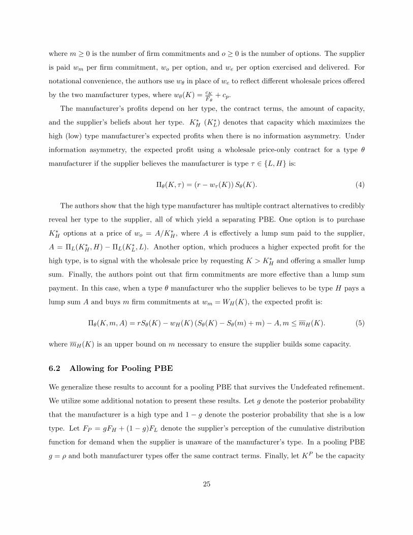
where m ≥ 0 is the number of firm commitments and o ≥ 0 is the number of options. The supplier

is paid wm per firm commitment, wo per option, and we per option exercised and delivered. For

notational convenience, the authors use wθ in place of we to reflect different wholesale prices offered

by the two manufacturer types, where wθ(K) = cKF θ

+ cp.

The manufacturer’s profits depend on her type, the contract terms, the amount of capacity,

and the supplier’s beliefs about her type. K∗H (K∗L) denotes that capacity which maximizes the

high (low) type manufacturer’s expected profits when there is no information asymmetry. Under

information asymmetry, the expected profit using a wholesale price-only contract for a type θ

manufacturer if the supplier believes the manufacturer is type τ ∈ {L,H} is:

Πθ(K, τ) = (r − wτ (K))Sθ(K). (4)

The authors show that the high type manufacturer has multiple contract alternatives to credibly

reveal her type to the supplier, all of which yield a separating PBE. One option is to purchase

K∗H options at a price of wo = A/K∗H , where A is effectively a lump sum paid to the supplier,

A = ΠL(K∗H , H) − ΠL(K∗L, L). Another option, which produces a higher expected profit for the

high type, is to signal with the wholesale price by requesting K > K∗H and offering a smaller lump

sum. Finally, the authors point out that firm commitments are more effective than a lump sum

payment. In this case, when a type θ manufacturer who the supplier believes to be type H pays a

lump sum A and buys m firm commitments at wm = WH(K), the expected profit is:

Πθ(K,m,A) = rSθ(K)− wH(K) (Sθ(K)− Sθ(m) +m)−A,m ≤ mH(K). (5)

where mH(K) is an upper bound on m necessary to ensure the supplier builds some capacity.

6.2 Allowing for Pooling PBE

We generalize these results to account for a pooling PBE that survives the Undefeated refinement.

We utilize some additional notation to present these results. Let g denote the posterior probability

that the manufacturer is a high type and 1 − g denote the posterior probability that she is a low

type. Let FP = gFH + (1 − g)FL denote the supplier’s perception of the cumulative distribution

function for demand when the supplier is unaware of the manufacturer’s type. In a pooling PBE

g = ρ and both manufacturer types offer the same contract terms. Finally, let KP be the capacity

25

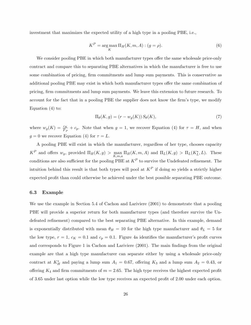
investment that maximizes the expected utility of a high type in a pooling PBE, i.e.,

KP = arg maxK

ΠH(K,m,A) : (g = ρ). (6)

We consider pooling PBE in which both manufacturer types offer the same wholesale price-only

contract and compare this to separating PBE alternatives in which the manufacturer is free to use

some combination of pricing, firm commitments and lump sum payments. This is conservative as

additional pooling PBE may exist in which both manufacturer types offer the same combination of

pricing, firm commitments and lump sum payments. We leave this extension to future research. To

account for the fact that in a pooling PBE the supplier does not know the firm’s type, we modify

Equation (4) to:

Πθ(K, g) = (r − wg(K))Sθ(K), (7)

where wg(K) = cKFP

+ cp. Note that when g = 1, we recover Equation (4) for τ = H, and when

g = 0 we recover Equation (4) for τ = L.

A pooling PBE will exist in which the manufacturer, regardless of her type, chooses capacity

KP and offers wg, provided ΠH(K, g) > maxK,m,a

ΠH(K,m,A) and ΠL(K, g) > ΠL(K∗L, L). These

conditions are also sufficient for the pooling PBE at KP to survive the Undefeated refinement. The

intuition behind this result is that both types will pool at KP if doing so yields a strictly higher

expected profit than could otherwise be achieved under the best possible separating PBE outcome.

6.3 Example

We use the example in Section 5.4 of Cachon and Lariviere (2001) to demonstrate that a pooling

PBE will provide a superior return for both manufacturer types (and therefore survive the Un-

defeated refinement) compared to the best separating PBE alternative. In this example, demand

is exponentially distributed with mean θH = 10 for the high type manufacturer and θL = 5 for

the low type, r = 1, cK = 0.1 and cp = 0.1. Figure 4a identifies the manufacturer’s profit curves

and corresponds to Figure 1 in Cachon and Lariviere (2001). The main findings from the original

example are that a high type manufacturer can separate either by using a wholesale price-only

contract at K∗H and paying a lump sum A1 = 0.67, offering K3 and a lump sum A2 = 0.43, or

offering K4 and firm commitments of m = 2.65. The high type receives the highest expected profit

of 3.65 under last option while the low type receives an expected profit of 2.00 under each option.

26

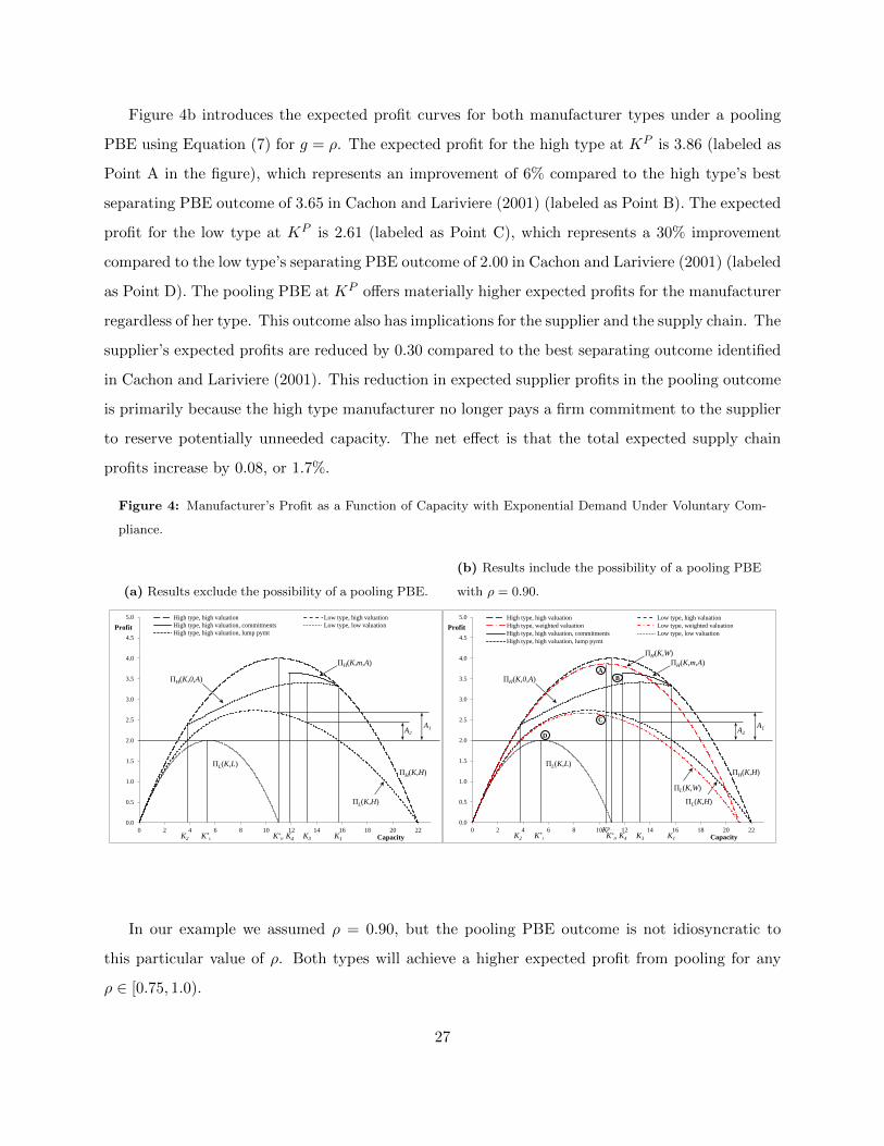
Figure 4b introduces the expected profit curves for both manufacturer types under a pooling

PBE using Equation (7) for g = ρ. The expected profit for the high type at KP is 3.86 (labeled as

Point A in the figure), which represents an improvement of 6% compared to the high type’s best

separating PBE outcome of 3.65 in Cachon and Lariviere (2001) (labeled as Point B). The expected

profit for the low type at KP is 2.61 (labeled as Point C), which represents a 30% improvement

compared to the low type’s separating PBE outcome of 2.00 in Cachon and Lariviere (2001) (labeled

as Point D). The pooling PBE at KP offers materially higher expected profits for the manufacturer

regardless of her type. This outcome also has implications for the supplier and the supply chain. The

supplier’s expected profits are reduced by 0.30 compared to the best separating outcome identified

in Cachon and Lariviere (2001). This reduction in expected supplier profits in the pooling outcome

is primarily because the high type manufacturer no longer pays a firm commitment to the supplier

to reserve potentially unneeded capacity. The net effect is that the total expected supply chain

profits increase by 0.08, or 1.7%.

Figure 4: Manufacturer’s Profit as a Function of Capacity with Exponential Demand Under Voluntary Com-

pliance.

(a) Results exclude the possibility of a pooling PBE.

0.0

0.5

1.0

1.5

2.0

2.5

3.0

3.5

4.0

4.5

5.0

0 2 4 6 8 10 12 14 16 18 20 22

Profit

Capacity

High type, high valuation Low type, high valuation

High type, high valuation, commitments Low type, low valuation

High type, high valuation, lump pymt

K*L K*

H K1K3K2 K4

A1A2

ΠH(K,m,A)

ΠH(K,0,A)

ΠH(K,H)

ΠL(K,H)

ΠL(K,L)

(b) Results include the possibility of a pooling PBE

with ρ = 0.90.

0.0

0.5

1.0

1.5

2.0

2.5

3.0

3.5

4.0

4.5

5.0

0 2 4 6 8 10 12 14 16 18 20 22

Profit

Capacity

High type, high valuation Low type, high valuation

High type, weighted valuation Low type, weighted valuation

High type, high valuation, commitments Low type, low valuation

High type, high valuation, lump pymt

K*L K*

H K1

Kp

K3K2 K4

A1A2D

C

B

A

ΠH(K,m,A)

ΠH(K,0,A)

ΠH(K,H)

ΠL(K,H)

ΠL(K,L)

ΠH(K,W)

ΠL(K,W)

In our example we assumed ρ = 0.90, but the pooling PBE outcome is not idiosyncratic to

this particular value of ρ. Both types will achieve a higher expected profit from pooling for any

ρ ∈ [0.75, 1.0).

27

6.4 Applications to Other Research

We note that the results of other research streams can be extended by explicitly considering pooling

outcomes through the application of the Undefeated refinement. These research streams include

supply chain coordination and contracting (Ozer and Wei 2006), franchising decisions (Desai and

Srinivasan 1995), channel stuffing (Lai et al. 2011), and market encroachment by suppliers (Li et al.

2014). The outcome examined in each of these papers is the least cost separating PBE. In each

case, however, a pooling PBE exists and survives the Undefeated refinement across some set of

model parameters. We leave a detailed analysis of the implications of applying the Undefeated

refinement in these settings to future research.

7 Opportunities for Future Research

Our experimental analysis is intended to test the predictive power of common equilibrium assump-

tions made in signaling games, not to provide a behavioral explanation of why some equilibrium

assumptions are more predictive than others. It may be that decision makers are influenced by

behavioral factors that align with the predictions of the Undefeated refinement. Behavioral expla-

nations may include the use of cognitive hierarchy models (Camerer et al. 2004), payoff disparity

comparisons (Ho and Weigelt 1996), or risk seeking and risk aversion tradeoffs (Holt and Laury

2002). Developing a better understanding of the behavioral mechanisms that lead to certain de-

cisions under information asymmetry will not only provide insights into the boundary conditions

on when the various refinements are more appropriate, but may also lead to the development of

improved equilibrium refinement assumptions. We leave this investigation for future research.

8 Implications and Conclusions

Our findings provide the first evidence that when pooling equilibria exist, they can be more pre-

dictive of operations management decisions made under information asymmetry than the more

commonly studied least cost separating equilibria. The predicted outcomes in our setting, and

from signaling game models generally, can yield materially different results and are sensitive to

equilibrium assumptions, specifically whether the Undefeated refinement or the Intuitive Criterion

refinement is applied. Testing the predictive power of these assumptions is therefore important.

28

While decision making under information asymmetry is a burgeoning field within operations

management, little has been done to reconcile the assumptions that underlie models in this area

with the choices of actual decision makers. The primary contribution of this paper is to provide

empirical evidence that characterizes the types of decisions made by actors in these contexts. In our

experiment, pooling outcomes, which are not regularly considered in the literature, were widespread

among participants, relative to separating outcomes. In particular, averaged across all scenarios,

participant choices were three times more likely to conform with the Undefeated refinement, which

allows for pooling equilibria, than the Intuitive Criterion refinement, which does not, and to date

has been the predominant belief refinement used in the operations management literature. These

results can inform the development of operations management theory, as well as help practitioners

interpret the implications of models that emerge from our field.

We observe several patterns in our data that provide confidence that the conformance with

the Undefeated refinement that we observe in the laboratory may extend to the decision-making

choices of real managers. First, we expect that prudent managers would make deliberate decisions

in practice, paying attention to changing dynamics and responding rationally to changes in the

underlying payoff structure. We observe such actions in our experiment, wherein participants’ de-

cisions corresponded with changes in the underlying newsvendor unit price, which suggests that

participants were paying attention to the stimuli and being thoughtful about their decisions. Sec-

ond, in practice, we expect actual decision makers to possess a deep understanding of the decision

space and the implications of their decisions. Consistently, in our experiment, we observe that

participants who report a high level of understanding of the setting are significantly more likely to

make choices that are consistent with the Undefeated refinement than participants who report a

low level of understanding. Third, we expect managers to use strategies that generate higher pay-

offs. In our experiment, participants who made choices that were consistent with the Undefeated

refinement earned higher payoffs from investors on average than participants who made choices that

were consistent with the Intuitive Criterion refinement. This is particularly interesting in the con-

text of our experiment, in which participants engaged in decisions from both the investor and firm

perspectives and were exposed to the full set of incentives afforded to both sides. Finally, we would

expect that over time, experienced managers would increasingly gravitate toward the strategy that

returns the highest payoff. Indeed, in our experiment, while participant choices overwhelmingly

29

conformed with the predictions of the Undefeated refinement, even during the first rounds of game

play, the tendency to make such choices intensified as participants experienced more rounds of the

game. As the order in which scenarios were presented was counterbalanced across sessions, the

pattern of these results is consistent with participants learning the efficacy of various strategies

and converging on the most successful strategies over time. All of these patterns observed among

the participants in our experiment are consistent with the actions of managers in practice, which

increases our confidence about the generalizability of our results.

Managers are constantly operating under conditions of information asymmetry. The decisions

they make can send signals about their firms’ prospects to less-informed parties in a broad array

of contexts. From a manager evaluating the viability of a potential supply chain partner, to

a customer evaluating a firm’s ability to meet her needs, to an analyst developing guidance on

a firm’s future stock performance, the signals firms send through their actions can materially

influence how they are perceived and engaged by less-informed parties, with important implications

for both sides. We expect this growing area of operations management research to continue to

flourish. To the extent our results expand the set of anticipated managerial choices in these contexts,

exploring their operational implications through the application of the Undefeated refinement may

enrich the extant theory. Opportunities exist to revisit established models, explore the implications

of equilibrium assumptions in new settings, and empirically examine managerial decisions and

outcomes under information asymmetry. Furthermore, future experimental work may unpack the

behavioral drivers underlying various equilibria among the parties in these settings, as well as their

corresponding boundary conditions. We leave these promising lines of inquiry to future research.

References

Anand, Krishnan S., Manu Goyal. 2009. Strategic information management under leakage in a supply chain.

Management Science 55(3) 438–452.

Banks, Jeffrey, Colin Camerer, David Porter. 1994. An experimental analysis of Nash refinements in signaling

games. Games and Economic Behavior 6(1) 1–31.

Barton, Dominic. 2011. Capitalism for the long term. Harvard Business Review March 2011 3–9.

Bebchuk, Lucian Arye, Lars A. Stole. 1993. Do short-term objectives lead to under- or overinvestment in

long-term projects? The Journal of Finance 48(2) 719–729.

30

Bolton, Gary E., Elena Katok. 2008. Learning by doing in the newsvendor problem: A laboratory investiga-

tion of the role of experience and feedback. Manufacturing and Service Operations Management 10(3)

519 – 538.

Bolton, Patrick, M. Dewatripont. 2005. Contract theory . MIT Press, Cambridge, Mass.

Bostian, A.J., Charles A. Holt, Angela M. Smith. 2008. Newsvendor “pull-to-center” effect: Adaptive

learning in a laboratory experiment. Manufacturing and Service Operations Management 10(4) 590 –

608.

Brandts, Jordi, Gary Charness. 2011. The strategy versus the direct-response method: A first survey of

experimental comparisons. Experimental Economics 14(3) 375–398.

Brandts, Jordi, Charles A. Holt. 1992. An experimental test of equilibrium dominance in signaling games.

The American Economic Review 82(5) 1350–1365.

Brandts, Jordi, Charles A Holt. 1993. Adjustment patterns and equilibrium selection in experimental sig-

naling games. International Journal of Game Theory 22(3) 279–302.

Brandts, Jordi, Charles A Holt. 1996. Naive bayesian learning and adjustment to equilibrium in signaling

games. Journal of Economic Behavior and Organization .

Bruns, Jr., William J., Kenneth A. Merchant. 1990. The dangerous morality of managing earnings. Man-

agement Accounting 72(2) 22–25.

Cachon, Gerard P., Martin A. Lariviere. 2001. Contracting to assure supply: How to share demand forecasts

in a supply chain. Management Science 47(5) 629–646.

Camerer, Colin F, Teck-Hua Ho, Juin-Kuan Chong. 2004. A cognitive hierarchy model of games. The

Quarterly Journal of Economics 861–898.

Cho, In-Koo, David M. Kreps. 1987. Signaling games and stable equilibria. The Quarterly Journal of

Economics 102(2) 179–221.

Cooper, David J., Susan Garvin, John H. Kagel. 1997. Signalling and adaptive learning in an entry limit

pricing game. RAND Journal of Economics 28(4) 662 – 683.

Debo, Laurens, Senthil Veeraraghavan. 2010. Prices and congestion as signals of quality. Working paper,

Chicago Booth School of Business, University of Chicago.

Desai, Preyas S., Kannan Srinivasan. 1995. Demand signalling under unobservable effort in franchising:

Linear and nonlinear price contracts. Management Science 41(10) 1608–1623.

Fishman, Michael J, Kathleen M Hagerty. 2003. Mandatory versus voluntary disclosure in markets with

informed and uninformed customers. Journal of Law, Economics, and Organization 19(1) 45–63.

Fudenberg, Drew, Jean Tirole. 1991. Game theory . MIT Press, Cambridge, Mass.

31

Gomes, Armando. 2000. Going public without governance: Managerial reputation effects. The Journal of

Finance 55(2) 615–646.

Graham, John R., Campbell R. Harvey, Shiva Rajgopal. 2005. The economic implications of corporate

financial reporting. Journal of Accounting and Economics 40(1-3) 3–73.

Ho, Teck-Hua, Keith Weigelt. 1996. Task complexity, equilibrium selection, and learning: An experimental

study. Management Science 42(5) 659–679.

Holmstrom, Bengt. 1999. Managerial incentive problems: A dynamic perspective. The Review of Economic

Studies 66(1) 169–182.

Holt, Charles A, Susan K Laury. 2002. Risk aversion and incentive effects. The American Economic Review

92(5) 1644–1655.

Islegen, Ozge, Erica L. Plambeck. 2007. Capacity leadership in supply chains with asymmetric demand

information and noncontractible capacity. Working Paper, Stanford Graduate School of Business.

Kremer, Mirko, Stefan Minner, Luk N. Van Wassenhove. 2010. Do random errors explain newsvendor

behavior? Manufacturing and Service Operations Management 12(4) 673–681.

Kreps, David M., Joel Sobel. 1992. Signalling. Robert J. Aumann, Sergiu Hart, eds., Handbook of Game

Theory with Economic Applications, vol. 11, chap. 25. North-Holland; Elsevier Science Pub. Co., Am-

sterdam; New York, N.Y., 850–867.

Lai, Guoming, Laurens Debo, Lin Nan. 2011. Channel stuffing with short-term interest in market value.

Management Science 57(2) 332–346.

Lai, Guoming, Wenqiang Xiao, Jun Yang. 2012. Supply chain performance under market valuation: An

operational approach to restore efficiency. Management Science 58(10) 1933–1951.

Lariviere, Martin A., V. Padmanabhan. 1997. Slotting allowances and new product introductions. Marketing

Science 16(2) 112–128.

Li, Zhuoxin, Stephen M Gilbert, Guoming Lai. 2014. Supplier encroachment under asymmetric information.

Management Science 60(2) 449–462.

Mailath, George J., Masahiro Okuno-Fujiwara, Andrew Postlewaite. 1993. Belief-based refinements in sig-

nalling games. Journal of Economic Theory 60(2) 241–276.

Mas-Colell, Andreu, Michael Dennis Whinston, Jerry R. Green. 1995. Microeconomic theory . Oxford Uni-

versity Press, New York.

Narayanan, M. P. 1985. Managerial incentives for short-term results. The Journal of Finance 40(5) 1469–

1484.

Ozer, Ozalp, Wei Wei. 2006. Strategic commitments for an optimal capacity decision under asymmetric

forecast information. Management Science 52(8) 1238–1257.

32

Riley, John G. 2001. Silver signals: Twenty-five years of screening and signaling. Journal of Economic

Literature 39(2) pp. 432–478.

Roth, Alvin. 1995. Bargaining experiments. J. Kagel, A. Roth, eds., Handbook of experimental economics.

Princeton University Press, Princeton, NJ, 253–348.

Salanie, Bernard. 2005. The economics of contracts : A primer . 2nd ed. MIT Press, Cambridge, Mass.

Schmidt, William, Vishal Gaur, Richard Lai, Ananth Raman. 2015. Signaling to partially informed investors

in the newsvendor model. Production and Operations Management 24(3) 383–401.

Schweitzer, Maurice E., Gerard P. Cachon. 2000. Decision bias in the newsvendor problem with a known

demand distribution: Experimental evidence. Management Science 46(3) 404–420.

Spiegel, Yossef, Daniel F. Spulber. 1997. Capital structure with countervailing incentives. The RAND

Journal of Economics 28(1) pp. 1–24.

Stein, Jeremy C. 2003. Agency, information and corporate investment. George M. Constantinides, Milton

Harris, Rene M. Stulz, eds., Handbook of the economics of finance, vol. 21, 1st ed., chap. 2. Elsevier

North-Holland, Amsterdam; Boston, 110–163.

Taylor, Curtis R. 1999. Time-on-the-market as a sign of quality. The Review of Economic Studies 66(3)

555–578.

33

Table 1: The model parameters used to generate the six scenarios in the experiment.

Scenario µS µB σ2 p b w β 1− λ Q

1 6.0 6.25 0.15 0.75 0.05 0.40 0.60 0.35 100

2 6.0 6.25 0.15 0.80 0.05 0.40 0.60 0.35 100

3 6.0 6.50 0.15 0.75 0.05 0.40 0.60 0.35 200

4 6.0 6.50 0.15 0.80 0.05 0.40 0.60 0.35 200

5 6.0 6.25 0.15 0.85 0.00 0.40 0.55 0.35 100

6 6.0 6.25 0.15 0.90 0.00 0.40 0.55 0.35 100

Table 2: Summary of the Undefeated refinement and Intuitive Criterion refinement predictions for each scenario.

Scenario:1 2 3 4 5 6

Undefeated Pool on 5 Pool on 5 Pool on 6 Pool on 6 Pool on 5 Pool on 5

Intuitive Criterion Separating Separating Separating Separating Separating Separating

Table 3: Distribution of participants for categorical variables

Education Level Frequency Percent

High School 21 9.21Some College 114 50.00Bachelor’s 48 21.05Graduate / Professional 41 17.98Other / Missing 4 1.75

Total 228 100

Ethnicity Frequency Percent

African American 33 14.47Asian 46 20.18Caucasian 107 46.93Hispanic 18 7.89Other / Missing 24 10.53

Total 228 100

Session Frequency Percent

1 34 14.912 36 15.793 36 15.794 36 15.795 30 13.166 32 14.047 24 10.53

Total 228 100

34

Table 4: The proportion of participant decisions predicted by the Undefeated and Intuitive Criterion refine-ments.

Scenario:1 2 3 4 5 6 Total

Undefeated 71.1%*** 59.7%*** 63.2%*** 55.7%*** 71.1%*** 60.5%*** 63.5%***Difference 11.4%* 7.5% 10.5%*

Intuitive Criterion 17.1%*** 29.4% 17.1%*** 25.9%* 15.8%*** 20.6%*** 20.9%***Difference -12.3%** -8.8%* -4.8%

Observations 228 228 228 228 228 228 1,368

Notes: The percentages in row 1 identify the proportion of participants whose choices conform to theUndefeated refinement. The percentages in row 2 are the difference between the percentages in row 1 forscenarios 1 and 2, 3 and 4, and 5 and 6. The percentages in row 3 identify the proportion of participantswhose choices conform to the Intuitive Criterion refinement. The percentages in row 4 are the differencebetween the percentages in row 3 for scenarios 1 and 2, 3 and 4, and 5 and 6. The symbols in rows 1and 3 identify whether the values are statistically significantly different from 33.333%. The symbols inrows 2 and 4 identify whether the values are statistically significantly different from 0%. All test aremade using two-tail binomial tests with *** p <0.001, ** p <0.01, * p <0.05, and + p <0.10.

Table 5: The proportion of participant decisions which comply to the Undefeated refinement, differentiated byfirm type.

Scenario:1 2 3 4 5 6

“Big” Type 68.9%*** 49.6%*** 61.5%*** 47.3%*** 64.0%*** 53.8%***Difference 19.3%*** 14.2%* 10.2%+

Observations 148 141 148 150 150 158

“Small” Type 75.0%*** 75.9%*** 66.3%*** 71.8%*** 84.6%*** 75.7%***Difference 0.9% -5.5% 8.9%

Observations 80 87 80 78 78 70

Notes: The percentages in row 1 identify the proportion of “Big” type firms whose choicesconform to the Undefeated refinement. The percentages in row 2 are the difference betweenthe percentages in row 1 for scenarios 1 and 2, 3 and 4, and 5 and 6. The percentages in row4 identify the proportion of “Small” type firms whose choices conform to the Undefeatedrefinement. The percentages in row 5 are the difference between the percentages in row 4for scenarios 1 and 2, 3 and 4, and 5 and 6. The symbols in rows 1 and 4 identify whetherthe values are statistically significantly different from 33.333%. The symbols in rows 2 and5 identify whether the values are statistically significantly different from 0%. All test aremade using two-tail binomial tests with *** p <0.001, ** p <0.01, * p <0.05, and + p <0.10.

35

Table 6: Description of Variables

Variable Description

Undefeated Indicator variable identifying whether the Undefeated re-finement predicts the firm’s choice (‘1’) or not (‘0’)

Intuitive Indicator variable identifying whether the Intuitive Crite-rion refinement predicts the firm’s choice (‘1’) or not (‘0’)

Payoff Payoff (in dollars) the participant received in the round

Understanding Indicator variable identifying whether the participant ratedtheir understanding as a ‘5’ or higher (‘1’), or a ‘4’ or lower(‘0’) on a 7-point Likert scale where ‘1’ indicates “I did notunderstand the game at all” and ‘7’ indicates “I understoodthe game completely”

Understanding - No Response Indicator variable identifying whether the participant ratedtheir understanding (‘1’) or not (‘0’)

Big Indicator variable identifying whether the participant’s firmis a Big type in current round (‘1’) or a Small type (‘0’)

Switch Indicator variable identifying whether the participant’s finalchoice deviates from their initial strategy (‘1’) or not (‘0’)

Session Categorical variable identifying the experimental session

Sequence Categorical variable identifying the sequence in which a sce-nario was presented to the participant

Age Participant’s age

Female Indicator variable identifying whether the participant is fe-male (‘1’) or male (‘0’)

Ethnicity Categorical variable indicating whether the participant isAfrican-American, Asian, Caucasian, Hispanic, Pacific Is-lander, or Other

Education Categorical variable indicating whether the participant hasa high school diploma, some college, a bachelors degree, oran advanced degree

ESL Indicator variable identifying whether English is partici-pant’s second language (‘1’) or primary language (‘0’)

Notes : Understanding, and demographic variables (Age through ESL) are dimensioned by partici-pant. All other variables are dimensioned by participant-round.

36

Table 7: Summary Statistics and Correlations

Variables Mean Std. Dev. Min. Max. N Un

def

eate

d

Intu

itiv

e

Payoff

Un

der

stan

din

g

Big

Sw

itch

Age

Fem

ale

ES

L

Undefeated 0.64 0.48 0 1 1368 1.00Intuitive 0.21 0.41 0 1 1368 -0.68 1.00Payoff 0.85 0.21 0.02 1.27 1368 0.06 -0.12 1.00Understanding 0.86 0.35 0 1 1368 0.14 -0.16 0.07 1.00Big 0.65 0.48 0 1 1368 -0.17 0.07 0.51 0.02 1.00Switch 0.11 0.31 0 1 1368 -0.12 0.05 -0.02 -0.07 -0.04 1.00Age 25.43 9 18 63 1278 -0.15 0.18 -0.04 -0.15 0.02 -0.04 1.00Female 0.48 0.5 0 1 1362 0.00 -0.03 -0.01 -0.08 -0.04 0.06 -0.16 1.00ESL 0.11 0.31 0 1 1362 -0.00 0.03 -0.00 -0.02 -0.05 -0.08 0.03 -0.00 1.00

37

Table 8: Estimating whether the predictive powers of the Undefeated and Intuitive Criterion refinements areassociated with the participant’s self-reported Understanding of the game.

(1) (2)Dependent Variable: Undefeated Intuitive

Coefficient OR Coefficient OR

Understanding 0.68* 1.97* -0.91*** 0.40***[0.28] [0.56] [0.27] [0.11]

Understanding - No Response -0.50 0.61 -1.61+ 0.20+[0.94] [0.57] [0.94] [0.19]

Big -0.93*** 0.39*** 0.42* 1.52*[0.17] [0.07] [0.19] [0.29]

Switch -0.83*** 0.44*** 0.44+ 1.56+[0.22] [0.10] [0.23] [0.36]

Constant 1.01* 2.74* -1.25* 0.29*[0.48] [1.33] [0.51] [0.15]

Observations 1,368 1,368Pseudo R2 0.11 0.09Mean DV 0.64 0.21Hosmer and Lemeshow χ2 12.63 5.94Hosmer and Lemeshow p-value 0.13 0.65Wald χ2 22.46***

Notes: Logistic estimation with robust standard errors clustered by participant in brackets.Included controls – Session, Sequence, Age, Female, Ethnicity, Education, and ESL. TheHosmer and Lemeshow χ2 test is based off of 10 groupings of the predictor variables. Alarge p-value for this test indicates a good model fit. Wald χ2 provides a test of theequivalency of the coefficient on Understanding across models (1) and (2). *** p <0.001,** p <0.01, * p <0.05, + p <0.10

Table 9: Estimating whether the participant’s payoff depends on their choice being predicted by the Undefeatedrefinement or the Intuitive Criterion refinement.

Dependent Variable: Payoff(1)

(A) Undefeated 0.04**[0.01]

(B) Intuitive -0.05***[0.01]

Understanding 0.01[0.01]

Understanding - No Response -0.02[0.03]

Big 0.23***[0.01]

Switch 0.02[0.01]

Constant 0.62***[0.02]

Observations 1,368R2 0.38Mean DV 0.85Wald F : (A)-(B)=0? 67.37***

Notes: OLS estimation with robust standard errors clustered by participantin brackets. Included controls – Session, Sequence, Age, Female, Ethnicity,Education, Student, and ESL. Wald tests report F statistics. *** p <0.001, **p <0.01, * p <0.05, + p <0.10

38

Appendix

Extensive Form Representations

Figure 5: Extensive form of Scenarios 3 and 4.

(a) Firm and investor payoffs for Scenario 3. Thereis a 35% probability that the participant in the roleof the firm is randomly assigned to be a “Small” op-portunity type firm.

(b) Firm and investor payoffs for Scenario 4. Thereis a 35% probability that the participant in the roleof the firm is randomly assigned to be a “Small” op-portunity type firm.

Figure 6: Extensive form of Scenarios 5 and 6.

(a) Firm and investor payoffs for Scenario 5. Thereis a 35% probability that the participant in the roleof the firm is randomly assigned to be a “Small” op-portunity type firm.

(b) Firm and investor payoffs for Scenario 6. Thereis a 35% probability that the participant in the roleof the firm is randomly assigned to be a “Small” op-portunity type firm.

39

Participant Instructions Script

The script read to all participants in the experiment is below.Slide 1. Welcome. I will first take you through an overview of the game that you will play and then

walk you through an example that will describe exactly how you will play this game on the computer.Slide 2. In each round you will be randomly assigned to play either the role of a Firm or an Investor.

Firms and Investors will then be randomly and anonymously paired with different people in each round.Slide 3. Firms will either have a “Small” or “Big” market opportunity, which is just a measure of the

number of customers the Firm expects to have for its product or service. Both the Firm and Investor willknow the Firm’s likelihood of getting a “Small” or “Big” market opportunity, but only the Firm will knowfor sure its actual opportunity.

Slide 4. Knowing its market opportunity, the Firm will decide how many stores to open. The Firm’spayoff depends not only on this decision, but on the price the Investor sets for the Firm.

Slide 5. The Investor learns how many stores the Firm will open and sets a price for the Firm. TheInvestor’s payoff depends on setting a price close to the Firm’s actual value.

Slide 6. You will see a picture similar to this in each game you play. I will cover the information onthis picture. As I mentioned previously, in each round the Firm is randomly assigned either a “Big” marketopportunity or a “Small” market opportunity.

Slide 7. The Firm has three choices for the number of stores to open, depending on its marketopportunity. In this example, a “Big” opportunity Firm can choose to open 6, 7 or 8 stores while a “Small”opportunity Firm can choose to open 5, 6, or 7 stores. Note that your information is always in red and theother player’s information is in blue.

Slide 8. Depending on the Firm’s choice, the Investor has either no choice or three choices for whatprice to set for the Firm. In this example, only a Firm with a “Big” opportunity can open 8 stores, andonly Firm with a “Small” opportunity can open 5 stores. Note that both a “Big” and a “Small” opportunityFirm can open either 6 or 7 stores. If the Investor sees one of these choices the Investor must decide whetherto set a “Big”, “Small” or “Weighted” price to the Firm. A “Weighted” price is a weighted average price.

Slide 9. If you are a Firm, your payoff depends on the size of the opportunity, your store choice, andthe price the Investor sets. In this example, if a “Big” Firm chooses 8 stores it will get a payoff of $0.82. If,however, a “Big” Firm chooses 6 stores it will get a payoff of $1.08, $0.98 or $0.77 depending on whetherthe Investor sets a price of “Big”, “Weighted” or “Small”. Similarly, if a “Big” Firm chooses 7 stores it willget a payoff of $1.00, $0.88 or $0.62 depending on whether the Investor sets a price of “Big”, “Weighted” or“Small”.

Slide 10. If you are an Investor, your payoff depends on setting a price close to the Firm’s actual value.For instance, in this example if the Firm chooses 6 stores and the Investor sets a price of “Big”, the Investorwill receive a payoff of $1.00 if the Firm is “Big,” and a payoff of $0.34 if the Firm is instead “Small”.

Slide 11. When the game begins, you will be told on screen whether you are a Firm or an Investorand the chance the Firm has of getting a “Big” or “Small” market opportunity. You will see a graphic withthe choices and payoffs for your game. Firms and Investors will receive the same information and will beasked to define their strategies. If you are a Firm, you will be asked “If you faced a Big market opportunity,how many stores would you open?” and “If you faced a Small market opportunity, how many stores wouldyou open?”

Slide 12. If you are an Investor, you will be asked “If the Firm opened X stores, what price wouldyou give them?”

Slide 13. The Firm’s market opportunity is then randomly assigned and the Firm confirms their storequantity choice.

Slide 14. The Investor sees the Firm’s store quantity choice and confirms the price they want to giveto the Firm.

Slide 15. The Firm and Investor learn what their pay-outs are for the previous game. Firms andInvestors swap roles. Firms and Investors are randomly assigned to new partners. Firms are randomlyassigned a “Big” or “Small” opportunity and a new game begins with different choices and/or pay-outs.

Slide 16. In addition to your show-up fee, you will be paid the sum of all your individual payoffs fromthe money rounds at the end of today’s session. You should try to make as much money as possible. Youare not taking money from other players. You are playing with other people, and they can’t move forwardunless you move forward. Please make your decisions in a timely fashion, be thoughtful but move quickly. Ifyour screen is black it means you are waiting for another player to make a decision. One other thing, pleasedon’t close your browser, or press next, back or refresh on the browser, as this can disrupt the game. If youhave any questions during the practice rounds, please raise your hand, and one of us will come around andanswer your question. Thank you! You may now begin.

40