experimental evaluation of the modal parameters changes of

Experimental Evaluation of the Modal Parameters Changes of a Telescopic Bulk Dock Structure

Rubén L Boroschek K. Francisco J Hernández P.Civil Engineering Department. University of Chile. Blanco Encalada 2002 Piso 4.

[email protected]

Abstract

An experimental and analytical estimation of changing modals parameters of a 132 meters long telescopic 3D frame ship loading structure is presented in this article. The structure consists of an external 110 meters length 3D steel truss than can move in the horizontal plane and an internal 3D trust that works as an extending arm. The total combined length of the structure after full extension of the telescopic arm is 132 meters. The extension length of the arm changes continuously according to the ship position and loading conditions. Due to the redistribution of mass and rigidity, the modal parameters of the structure changes continuously. In some occasions due to the load rate and load weight, important vibrations occur in the system. In order to understand the reason for the apparent vibration amplification and to validate an analytical model for risk assessment of the structure, several ambient and forced vibration measurements were performed on the structure. To capture the space – frequency characteristic, time – frequency system identification techniques were evaluated and are presented in this paper. The time-frequency methods presented in this article are the Short Time Frequency Spectrum, the Hilbert-Huang Transform (HHT) and the Wigner-Ville distribution (WVD). Some of the advantages and difficulties for each method are indicated. It is concluded that it is possible to monitor and to reproduce analytically, the complex response of this structure.

Introduction

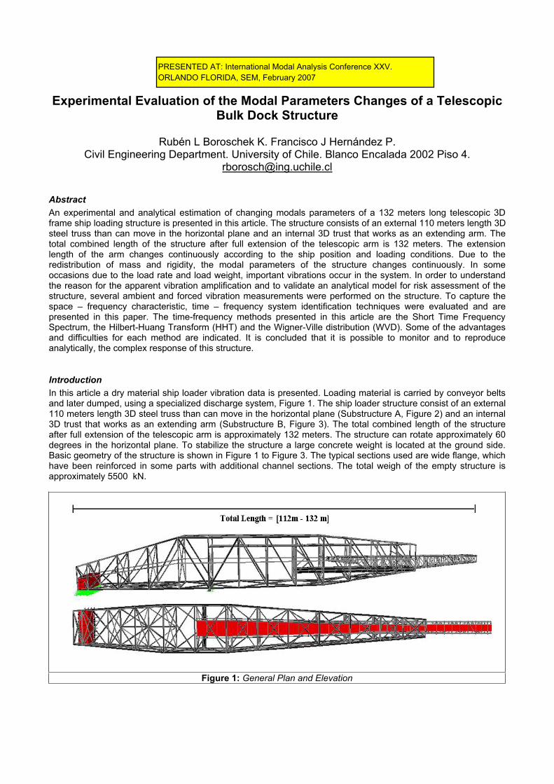
In this article a dry material ship loader vibration data is presented. Loading material is carried by conveyor belts and later dumped, using a specialized discharge system, Figure 1. The ship loader structure consist of an external 110 meters length 3D steel truss than can move in the horizontal plane (Substructure A, Figure 2) and an internal 3D trust that works as an extending arm (Substructure B, Figure 3). The total combined length of the structure after full extension of the telescopic arm is approximately 132 meters. The structure can rotate approximately 60 degrees in the horizontal plane. To stabilize the structure a large concrete weight is located at the ground side. Basic geometry of the structure is shown in Figure 1 to Figure 3. The typical sections used are wide flange, which have been reinforced in some parts with additional channel sections. The total weigh of the empty structure is approximately 5500 kN.

Figure 1: General Plan and Elevation

PRESENTED AT: International Modal Analysis Conference XXV.

ORLANDO FLORIDA, SEM, February 2007

Figure 2: Substructure A. Figure 3:Substructure B.

Due to dock characteristics the telescopic arm position changes continuously, according to ship position and loading condition. The radial and tangential position of the loading end is change by an operator located on the free end of the telescopic arm, just above the ship loading area. Under certain conditions of the loading material weight and rate of loading, the vibration of the structure is quite large making manoeuvring of the structure by the operator difficult.

The telescopic arm is supported on the main structure by mean of 8 wheels, with bottom and top rails attach to the substructure A. Top and bottom railing are separated by a distance slightly greater than the wheel diameter. This generates a single contact surface per wheel axis, top or bottom, depending on the telescopic arm position and loading characteristics. This gap an others structural conditions allow the telescopic arm to vibrate with relative large amplitudes when the loading discharge rate and structural modes are close enough to resonance.

Vibration Testing

Vibration testing of the structure had to be done with a maximum of 12 hours time and during loading of a single material type. Due to operation conditions and safety of the personnel only seven sensors where allowed to be place on top of the structure. Sensors where force balance accelerometers Model FBA – 11 and ES-U from Kinemetrics. Data acquisition system was IOTECH Model Daqbook 200. Sampling rate was set to 500 Hz and antialias filtering was set to 100 Hz. Five of the sensors where located on the telescopic arm. The other two sensors where located on the non telescopic part of the structure, Figure 4.

Figure 4: Sensor Location

Ambient Vibration and impact tests where performed at five different telescopic arm extensions, Table 1. Impact test were generated on the structure by jumping close to each sensor location. Additionally continuous forward and backward motion of the telescopic arm was monitor. Finally vibration data for different loading rates of dry material was measured. Loading rate monitored vary from 6000 to 10000 kN/hour in steps of 1000 kN/hour. In addition to vibration measurement, vibration perception was indicated by the operator located at the control cabin.

Data Analysis

Several ambient vibration records where obtained for different telescopic arm positions. Figure 5 show typical time records. Ambient vibrations are due to wind and operation in the areas close to the structure. As it can be observed, amplitudes are in the other of 0.002 g, nevertheless clear operational frequencies are observed. Predominant frequencies are estimated from the power spectra, transfer and correlation functions. For the power spectral analysis the Welch method is used, Figure 6.

Figure 5: Typical Ambient Vibration Records

Figure 6: Power Spectral Density and Coherence Function of Recorded Data

Ambient vibrations were monitor at different telescopic arm extension, 4.6, 9.6, 13.6, 18.5 and 22.4 meters. For each position, vibrations where recorded after the transient signal due to the extension of the arm have substantially decayed. Power Spectral Density (PSD) are shown in Figure 7 to Figure 10, for sensors located next to the control cabin (sensors 4 and 5) and at the end of substructure A (sensor 3). The PSD in this figures have been normalize. The predominant frequencies determined from the different positions and loading conditions are shown in Table 1. Frequency variations during different loading rate are close to 8%, for loading rates of 0 to 10000 kN/hour.

Several important features can be observed from figures and table:

1. The predominant frequency of the transverse motion varies from 0.64 to 0.71 Hz. 2. The predominant frequency of the vertical motion of the complete structure varies from 0.85 to 0.94 Hz.

The motion associated with this frequency, also has contribution in the horizontal plane, although they are smaller than in the vertical direction.

3. The second predominant vertical motion is mainly govern by the vibration of the telescopic arm (1.5 Hz). 4. An important characteristic of the motion is that when the arm is extending, the main predominant vertical

frequency diminishes, as seen in Figure 11. The larger the extension the larger the reduction in predominant frequency. (0,93 to 0,84 Hz)

5. On the contrary the second predominant vertical vibration that is dominated mainly by the telescopic arm does not have a proportional change with arm extension, Figure 12. For example for 4.6 meter predominant frequency is close to 1.52 Hz, for 18.5 meters predominant frequency is 1.55 Hz and for 22.4 m frequency is 1.50 Hz. These are not large variations for resonance study purposes, but large enough to be detected with this rather crude method. The reason for this non proportionality is because the telescopic arm is supported on wheels that move on rails that are supported every 6,9 or 9,1 meters by the vertical elements of the framing of substructure A. When the wheels are close to a vertical element then the rigidity of the railing systems decreases, modifying the motion frequency. In case that the telescopic arm was supported on an infinite rigid railing system, then the predominant frequency will not change. The importance of substructure A on this predominant vertical frequency is rather small, except for the local stiffness of its connecting elements with substructure B.

Figure 7: Power Spectral Density Substructure A. Sensor 1.

Figure 8: Power Spectral Density Substructure A. Sensor 3.

Figure 9: Power Spectral Density Substructure B. Sensor 6.

Figure 10: Power Spectral Density Substructure B. Sensor 5.

Figure 11: Power Spectral Density Frequency Variation as a Function of Position. Lower Frequency. Sensor 6.

Figure 12: Power Spectral Density Frequency Variation as a Function of Position. Higher Frequency. Sensor 6.

Damping was evaluated with three different methods ITD [1], Bandwidth and Stochastic Subspace Identification using Matlab n4sid routine [6]. ITD and SSI where also used to generate the information on predominant frequency. SSI was used on the same data set used for PSD studies. Figure 13 presents a stability diagram. As seen form Figure 11 and Figure 12, damping does not change considerably for the different positions. Nevertheless equivalent damping values change considerably due to inherent nonlinearities of the system due to traction system and wheel contact, depending on position and loading. Despite of this situation, it can be concluded that the horizontal motions have large damping, generally on the order of 5 to 10% and vertical motion that are more susceptible to material loading rate related amplifications are comparably small, 0.5 to 1.5%.

Figure 13: Stability Diagram

Continuous Monitoring of Predominant Frequency Variations

An interesting aspect of this evaluation is the possibility of continually monitor the predominant frequency variations of the system. There are several methods to estimate the frequency variation as a function of time. The simplest one is the Short Time Fourier Transform [2] and its squared value the spectrogram. This procedure plots a short time window Fourier transform of the data in a sequential form generating an estimate of amplitude – frequency – time. Figure 14 presents a record and its spectrogram obtained when the telescopic arm was extended from 4.6 to 22.4 meters, in 40 seconds. Figure 15 presents a 3D view of the spectrogram. The two predominant vertical frequencies are clearly observed. Figure 16 presents a spectrogram of a band filter signal around the lower vertical predominant frequency. A solid black line has been drawn following the maximum values. A clear frequency variation is observed from seconds 25 to 60. This value agrees with what was observed from the individual position of the telescopic arm. Figure 17 presents the frequency band corresponding to the second vertical predominant motion. In this case as observed previously, a clear tendency is not present, nevertheless variation are rather small. When the telescopic arm is contracted a similar but inverse trend is observed, Figure 18.

We are now in the process of evaluating other time-frequency representations. As example we show the Wigner Ville decomposition [2] and Hilbert-Huang Transform [3]. No description of the theory behind of these methods is

presented due to space limitations. The Wigner-Ville distribution of a signal ( )x t is defined by:

*1 1 1( , ) ( ) ( )

2 2 2

j wWV t w x t x t e d (1)

The Wigner-Ville distribution of acceleration record shown in Figure 14 and Figure 15 can be seen in Figure 19. The signal on the 0.8 - 0.95 frequency band is present with relative low amplitude. The second predominant vertical frequency, close to 1.5 Hz is clearly visible and defined. The frequency around 1.2 Hz is product of interference of the two signals. If the original acceleration record is low pass filtered, so that only the first

predominant frequency is present and the maximum value of frequency for each time step is selected, a good estimate of the instantaneous frequency of the signal is found, Figure 22.

The Hilbert-Huang Transform has two main steps. The first one separates a signal in apparent modes based on an enveloped sifting method call Empirical Mode Decomposition, Figure 20. Later the instantaneous frequency is found for each Empirical Mode, Figure 21.

The instantaneous frequency is defined by the following equation.

arg ( )1( )

2

ad x tf t

dt (2)

Where ( ) ( ) ( ( ))ax t x t jHT x t and ( ( ))HT x t is the Hilbert transform of ( )x t

From this last figure it is clear that the different Empirical Modes have components of frequencies of both real predominant frequencies, making a clear identification of the instantaneous frequency difficult.

In Figure 22 all the frequency estimates for the lower predominant frequency are shown.

Conclusion

The predominant vibration frequencies of a telescopic loading system are analyzed using different processing schemes.

The following are the main conclusion:

1. Despite the rather small frequency variation (11%) in a relative short time (40 seconds) it was possible to detect the change and to determine with enough accuracy its mean value as a function of time.

2. For this problem the Spectrogram gave a sufficiently reliable description of the frequency change in comparison with more mathematically complex and computer demanding procedures.

3. The Wigner-Ville distribution was able to show the predominant frequencies as a function of time but the computational effort was considerable.

4. The Hilbert-Huang Transform did not produce reliable results in this case due to the closeness of the predominant period and the level of noise of the records.

Figure 14: Spectrogram of Vertical Acceleration of Sensor 4. Telescopic Arm Extension.

Figure 15: 3D view of Spectrogram of Vertical Acceleration of Sensor 4. Telescopic Arm Extension.

Figure 16: Spectrogram of Vertical Acceleration of Sensor 4. Telescopic Arm Extension. Lower Frequencies.

Figure 17: Spectrogram of Vertical Acceleration of Sensor 4. Telescopic Arm Extension. Higher Frequencies.

Figure 18: Spectrogram of Vertical Acceleration of Sensor 4. Telescopic Arm Contraction

Figure 19: Wigner-Ville Distribution of Vertical Acceleration of Sensor 4. Telescopic Arm Extension

Figure 20: Empirical Mode Decomposition of Vertical Acceleration of Sensor 4. Telescopic Arm Extension

Figure 21: Empirical Mode and Instantaneous Frequency of Analytical Signal.

Figure 22: Comparison of Estimated Predominant Frequency as a Function of Time

Table 1: Predominant Frequency and Damping

Overhanging Distance 4,6 m

Direction Frequency [Hz]

Damping [%]

Frequency Analytic Model Unloaded Structure

[Hz]

Horizontal 0,667 [2,5 – 14,5 * ] 0.78

Vertical [0,933 - 0,938] [0,5 – 1,5] 0.91

Vertical [1,537 - 1,545] [0,5 – 1,5] 1.62

Horizontal [1,985 - 1,990] [0,5 – 1,5] 1.63



Damping [%]


[Hz]

Horizontal [0,661 - 0,644] [4,0 – 5,0] 0.74

Vertical [0.896 - 0,897] [0,5 – 1,5] 0.87

Vertical [1.546 - 1,549] [0,5 – 1,0] 1.57

Horizontal [2.023 - 2,027] [0,5 – 1,0] 1.59



Damping [%]


[Hz]

Horizontal [0,705 - 0,712] [3,5 – 5,0] 0.73

Vertical [0.866 - 0,887] [0,5 – 2,0] 0.85

Vertical 1,535 [0,5 – 1,0] 1.60

Horizontal [2,102 -2,107] [0,5 – 1,0] 1.64



Damping [%]


[Hz]

Horizontal [0,680 - 0,686] [2,0 – 4,0] 0.69

Vertical [0,871 - 0.873] [0,5 – 2,0] 0.83

Vertical [1.554 - 1,556] [0,5 – 1,0] 1.61

Horizontal 2,149 [1,0 – 1,5] 1.59



Damping [%]


[Hz]

Horizontal [0,643 - 0,652] [3,5 – 4,5] 0.67

Vertical [0,845 - 0,899] [1,5 – 2,0] 0.80

Vertical 1,502 [0,5 – 1,5] 1.55

Horizontal [2,108 - 2,110] [0,5 – 1,5] 1.58

Acknowledgement

This study was done in part with the support of the Civil Engineering Department of the University of Chile and Fondecyt 1000912.

References

[1] Ibrahim, S. R. and Mikulcik, E. C., "A method for the direct determination of vibration parameters from free responses," Shock and Vibration Bulletin, no. 47, part 4, September, 1977, pp. 183-198.

[2] Cohen, L “Time-Frequency Analysis”. Prentice Hall. 1995.

[3] Norden E. Huang, Zheng Shen, Steven R. Long, Manli C. Wu, Hsing H. Shih, Quanan Zheng, Nai-hyuan Yen,Chi Chao Tung and Henry H. Liu. “The empirical mode decomposition and the Hilbert Spectrum for nonlinear and non-stationary time series analysis”. Proceedings of the Royal Society London 1998; A, Vol. 454, pp. 903-995.

[4] Auger, F., Flandrin, P., Concalvès, P., Lemoine, O. “Time-Frequency Toolbox. For Use with Matlab”. 1996.

[5] Ljung. L, “System Identification Theory for the user”. 2nd Ed, PTR Prentice Hall, Upper Saddle River, N.J., 1999.

[6] Ljung, L. “System Identification Toolbox User’s Guide”. The MathWorks, Inc., Natick, MA, 2001.

[7] Rilling, G., Flandrin, P. and Gongalvès P., "On Empirical Mode Decomposition and its algorithms". IEEE-EURASIP Workshop on Nonlinear Signal and Image Processing, NSIP-03, June 2003

experimental evaluation of the modal parameters changes of

Documents