experimental evaluation of structural composites for blast …
TRANSCRIPT

EXPERIMENTAL EVALUATION OF STRUCTURAL
COMPOSITES FOR BLAST RESISTANT DESIGN
A thesis presented to the Faculty of the Graduate School
University of Missouri – Columbia
In Partial Fulfillment of the Requirements for the Degree
Masters of Science
In
Civil and Environmental Engineering
By
JOHN M. HOEMANN
Dr. Hani Salim, Thesis Supervisor
May 2007
The Undersigned, appointed by the Dean of the Graduate School, have examined the
thesis entitled.
EXPERIMENTAL EVALUATION OF STRUCTURAL
COMPOSITES FOR BLAST RESISTANT DESIGN
Presented by: John M. Hoemann
A candidate for the degree of Masters of Science in Civil and Environmental
Engineering, and hereby certify that in their opinion it is worthy of acceptance.

ii
ACKNOWLEDGEMENTS
I would like thank all those who have contributed to my support and education at the
University of Missouri – Columbia. A special thanks to Dr. Hani Salim who has personally put
forth a great effort in encouraging my work, as an advisor. Also want thank him for his respect
and guidance as a friend. Another thank you is extended to Dr. Sam Kiger, Director of the
National Center for Explosion Resistance Design (NCERD), for his expertise in the research.
I would like to thank Dr. Robert Dinan, from the US Air Force Research Laboratory,
Tyndall Air Force Base his assistance in acquiring and supervising this work. In addition I would
like to thank Mr. Jeff Fisher, Mr. Joe Jordan, and Mr. Bryan Bewick of Applied Research &
Assciates, Tyndall AFB office for engineering assistance.
Also I would like to thank the graduate and undergraduate research members of the
NCERD team for there assistance in various rolls throughout my academic carrier at the
University of Missouri. Graduate members: Aaron Sauiser, Eric Sullins, Jeff Jobe, John
Kennedy, Rhett Johnson, and Silas Fitmorous. Undergraduate member: Adam Alexander,
Chance Baragary, Jennifer Zans, Matt Oesch, Nick Harvey, and Tyler Oesch.
But especially I would like to thank my wife Ann for her constant support and
encouragement in my efforts. Likewise I would like to thank all of my family for being
supportive over my academic career. In addition I must recognize the support that my friends
have also shown me.

iii
TABLE OF CONTENTS
ACKNOWLEDGEMENTS............................................................................................................. ii
LIST OF FIGURES ......................................................................................................................... v
LIST OF TABLES........................................................................................................................viii
ABSTRACT………………………………………………………………………………………...ix
1. Introduction......................................................................................................................... 1
1.1. Need for Maneuverable Structures ................................................................... 1
1.2. Objective ........................................................................................................... 4
2. Background......................................................................................................................... 6
2.1. Panel Fabrication and Composition .................................................................. 6
2.2. Previous Honeycomb Composite FRP Research ............................................ 10
2.3. Dynamic Loading and Analysis Review......................................................... 12
3. Static Laboratory Testing and Resistance Functions ........................................................ 17
3.1. Laboratory Testing.......................................................................................... 17
3.2. Wall Panels Resistance Functions .................................................................. 25
3.3. Roof Panels Resistance Functions .................................................................. 29
3.4. Static Resistance Function Summary.............................................................. 31
4. Dynamic Response Predictions Under Blast Loadings..................................................... 32
4.1. Dynamic Predictions of Wall Panels .............................................................. 32
4.2. Roof Panel Predictions.................................................................................... 33
4.3. Prediction Summary........................................................................................ 35
5. Field Evaluation of FRP Wall Panels Subjected to Blast ................................................. 36
5.1. Field Test Setup .............................................................................................. 36
5.2. Field Test Results and Verification................................................................. 38
5.3. Conclusion ...................................................................................................... 50
iv
6. Field Evaluation of FRP Wall Panels Under Fragmentation ............................................ 52
6.1. Field Test Setup .............................................................................................. 52
6.2. Field Evaluation .............................................................................................. 54
6.3. Conclusion ...................................................................................................... 63
7. Roof Blast Panel Testing .................................................................................................. 64
7.1. Roof Blast Test Setup ..................................................................................... 64
7.2. Roof Testing Results and Evaluation.............................................................. 68
7.3. Roof Test Conclusion ..................................................................................... 76
8. Conclusions and Recommendations ................................................................................. 78
9. References......................................................................................................................... 80

v
LIST OF FIGURES
Figure 1.1 Concept........................................................................................................................... 3
Figure 2.1 Five orientation of scaled testing laboratory panels ....................................................... 8
Figure 2.2 Ideal blast loading......................................................................................................... 13
Figure 2.3 SDOF spring mass system............................................................................................ 14
Figure 2.4 Free body diagram of a unit element of the beam ........................................................ 15
Figure 3.1 Static testing schematic 4–point bending ..................................................................... 18
Figure 3.2 Failed parallel weak axis Panel P5W ........................................................................... 20
Figure 3.3 Failed parallel weak axis Panel P4W ........................................................................... 20
Figure 3.4 Failed parallel strong axis Panel P3S ........................................................................... 21
Figure 3.5 Failed parallel strong axis Panel P4S ........................................................................... 21
Figure 3.6 Failed right – angle weak axis Panel R2W................................................................... 22
Figure 3.7 Failed right – angle strong axis Panel R2S................................................................... 23
Figure 3.8 Laboratory data – parallel weak axis panels................................................................ 24
Figure 3.9 Laboratory data – parallel strong, right-angle weak and strong axis panels................. 25
Figure 3.10 Laboratory Panels P4W and P5W .............................................................................. 27
Figure 3.11 Idealized resistance function ...................................................................................... 29
Figure 3.12 16–point loading tree.................................................................................................. 30
Figure 3.13 Static resistance function for roof panels ................................................................... 31
Figure 4.1 Design curve for field Panel W2 and W4..................................................................... 33
Figure 4.2 Simplified blast loading for roof predictions................................................................ 34
Figure 4.3 Predicted dynamic response of FRP roof panels without sand overlay........................ 34
Figure 5.1 Wall panel – setup ........................................................................................................ 37
Figure 5.2 Standoff design curve ................................................................................................... 38
Figure 5.3 Wall panel – pretest ...................................................................................................... 40
vi
Figure 5.4 Post-test view of panels ................................................................................................ 40
Figure 5.5 Post-test Panel W2........................................................................................................ 41
Figure 5.6 Post-test view of Panel W2........................................................................................... 41
Figure 5.7 Post-test view of Panel W1........................................................................................... 42
Figure 5.8 Post-test view of Panel W1........................................................................................... 42
Figure 5.9 Post-test view of Panel W3........................................................................................... 43
Figure 5.10 Wall test schematic..................................................................................................... 45
Figure 5.11 Wall test overpressure at 35'....................................................................................... 46
Figure 5.12 Wall test reflected pressure gauge – R1 ..................................................................... 47
Figure 5.13 Wall test reflected pressure gauge – R2 ..................................................................... 47
Figure 5.14 Wall test reflected pressure gauge – R4 ..................................................................... 48
Figure 5.15 Displacement of Panel W1 ......................................................................................... 48
Figure 5.16 Displacement of Panel W2 ......................................................................................... 49
Figure 5.17 Displacement of Panel W3 ......................................................................................... 49
Figure 5.18 Displacement of Panel W4 ......................................................................................... 50
Figure 6.1 Fragmentation test arena layout.................................................................................... 53
Figure 6.2 Fragmentation test setup............................................................................................... 53
Figure 6.3 Mortar ........................................................................................................................... 54
Figure 6.4 Post detonation ............................................................................................................. 54
Figure 6.5 Post-test Panel F3 ......................................................................................................... 55
Figure 6.6 Post-test Panel F4 ......................................................................................................... 56
Figure 6.7 Post-test Panel F5 ......................................................................................................... 56
Figure 6.8 Post-test Panel F6 ......................................................................................................... 57
Figure 6.9 Fragment penetration process (a) Panel F3 and (b) Panel F6 ....................................... 58
Figure 6.10 Post-test Panel F3 view of depth of fragment penetration.......................................... 59
Figure 6.11 Post-test Panel F4 view of depth of fragment penetration.......................................... 59

vii
Figure 6.12 Post-test Panel F5 view of depth of fragment penetration.......................................... 60
Figure 6.13 Post-test Panel F6 view of depth of fragment penetration.......................................... 61
Figure 6.14 Front face of Panels F1 and F2 (RBS)........................................................................ 62
Figure 6.15 Rear faces of Panels F1 and F2 .................................................................................. 62
Figure 7.1 Charge placements........................................................................................................ 65
Figure 7.2 Roof panels – 30 feet standoff to block face ................................................................ 66
Figure 7.3 Roof panels – end view pretest..................................................................................... 66
Figure 7.4 Roof Test Schematic.................................................................................................... 67
Figure 7.5 Free field gauge FF1..................................................................................................... 69
Figure 7.6 Free field gauge FF2..................................................................................................... 70
Figure 7.7 Free field gauge FF3..................................................................................................... 70
Figure 7.8 Free field gauge FF4..................................................................................................... 71
Figure 7.9 Free field gauge FF5..................................................................................................... 71
Figure 7.10 Free field gauge FF6................................................................................................... 72
Figure 7.11 Free field gauge FF7................................................................................................... 72
Figure 7.12 Free field gauge FF8................................................................................................... 73
Figure 7.13 Displacement at nearest quarter-point Panel 2R......................................................... 73
Figure 7.14 Displacement at nearest quarter-point Panel 1R......................................................... 74
Figure 7.15 Displacement at mid-point Panel 2R .......................................................................... 74
Figure 7.16 Displacement at mid-point Panel 1R .......................................................................... 75
Figure 7.17 Displacement at furthest quarter-point Panel 2R........................................................ 75
Figure 7.18 Displacement at furthest quarter-point Panel 1R........................................................ 76

viii
LIST OF TABLES
Table 2.1 Field test panel descriptions............................................................................................. 9
Table 3.1 Lab testing results for scaled panels .............................................................................. 19
Table 5.1 Field wall panel test summary ....................................................................................... 46
Table 7.1 Field roof panel test summary........................................................................................ 69
ix
EXPERIMENTAL EVALUATION OF STRUCTURAL
COMPOSITES FOR BLAST RESISTANT DESIGN
John M. Hoemann
Dr. Hani Salim, Thesis Supervisor
ABSTRACT
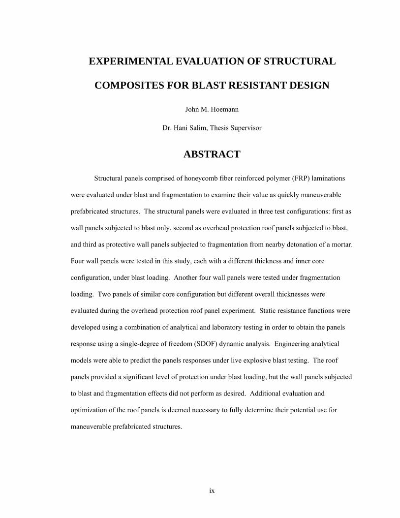
Structural panels comprised of honeycomb fiber reinforced polymer (FRP) laminations
were evaluated under blast and fragmentation to examine their value as quickly maneuverable
prefabricated structures. The structural panels were evaluated in three test configurations: first as
wall panels subjected to blast only, second as overhead protection roof panels subjected to blast,
and third as protective wall panels subjected to fragmentation from nearby detonation of a mortar.
Four wall panels were tested in this study, each with a different thickness and inner core
configuration, under blast loading. Another four wall panels were tested under fragmentation
loading. Two panels of similar core configuration but different overall thicknesses were
evaluated during the overhead protection roof panel experiment. Static resistance functions were
developed using a combination of analytical and laboratory testing in order to obtain the panels
response using a single-degree of freedom (SDOF) dynamic analysis. Engineering analytical
models were able to predict the panels responses under live explosive blast testing. The roof
panels provided a significant level of protection under blast loading, but the wall panels subjected
to blast and fragmentation effects did not perform as desired. Additional evaluation and
optimization of the roof panels is deemed necessary to fully determine their potential use for
maneuverable prefabricated structures.

1
1. Introduction
The United States Air Force (USAF) is always looking to identify pioneering ideas to
protect and advance soldiers. It is with ideas and the process of systematic research that progress
and innovation is accomplished. Every idea must be logically evaluated to reasonably compare
and argue its advantages or disadvantages to its application. This chapter will give the reader the
reasoning for why this research is needed and provide an outline for the presentation of this study.
1.1. Need for Maneuverable Structures
It is widely known that the United States is working to defend the nation by ways of
increasing security at airports, as well as installing barriers around federal buildings and parks in
order to provide a frontline to prevent terrorist attacks in our nation. Professional engineering
organizations are also stepping up by forming committees to develop design standards for
commercial and private buildings that engineers can utilize (Dusenberry, 2005). Dusenbarry
(2005) writes about the engineering need for blast design today; he recognizes the multiple areas
of which research and study will be needed to provide adequate information for the design of
structures. Similarly, international steps have been made in securing our foreign structures; US
embassy designs have advanced in the past 30 years in recognizing vulnerabilities in design
(Gurvin and Remson, 2001). Although these are examples of the need and attention that
engineers put on permanent structures, it is with this study that temporary structures will be
examined.
Gurvin and Remson (2001) study gives a timeline of security incidents that have plagued
the international facilities in the past, and how such incidents have brought about the need for
personnel access control (PAC). PAC is the idea that checkpoints along the perimeter or the
entrance of the facility will limit the attacker’s access to the most vulnerable parts of the

2
structure. One problem facing engineers is the need to protect the occupants of these
checkpoints; this is where a quickly maneuverable hardened structure would be ideal. US
embassies can go for sometime without having any threat levels that would pose any warning of a
possible attack. But either due to an international shift in power or a local incident the threat
level along the perimeter of an embassy can rapidly change. This rapid change in the level of
threat could lead to actions of securing a larger perimeter to insure enough standoff distance is
maintained for the facility, or if drastic action is needed to provide adequate cover for guards.
These are just two scenarios where maneuverable structures could be used. Traditional make-
shift sandbag bunkers are constructed as means for temporary protection during these heightened
threats.
Light-weight prefabricated temporary structures that can be assembled relatively easy in
the field are needed as an alternative to sandbag bunkers. Such structures need to be able to resist
a variety of blast and fragmentation threats. Due this, fiber-reinforced polymer (FRP) composites
are thought be ideal for prefabricated temporary structures with their high-strength-to-weight
ratio. This thesis will present the study of the FRP materials as wall and roof panels for these
temporary structures. In addition to the high-strength-to-weight ratio, FRP panels in general can
provide large amounts of flexibility that can provide the desired energy absorption capability to
resist blast loads. For added inertial resistance, the FRP panels can be filled with sand on-site to
provide additional blast and fragmentation protection. Figure 1.1 is a general schematic of the
concept for the temporary structures.

3
Figure 1.1 Concept
In addition, temporary structures can potentially be used in combat areas instead of
temporary field tents. The modular units could provide the structure and protection for barracks,
temporary hospitals, and command posts throughout any branch of service. USAF and all
Department of Defense (DOD) agencies are facing continued threats of insurgent attack in
combat areas. It is widely publicized that insurgent, a rebel against the political authority, attacks
are claming our soldiers. The tools that insurgents use are improvised explosive devices (IEDs)
which are homemade booby traps. IEDs are described as any commercial explosive that has been
modified, or homemade device with the addition of toxic chemicals, biologic toxins, radiological
material, or increased fragmentation properties that are engineered for a designated target (Global
Security, 2005). The site Global Security (2005) also recognizes that car and truck bombs can be
used as IEDs. With the insurgent and terrorist threats becoming a combination of blast and
fragments, it is important to observe both in an evaluation.
To improve the design and performance of any maneuverable structure, it is first
necessary to evaluate the materials and design looking for the most efficient blast and fragment
4
resistant system. Therefore, it is hypothesized in this study the honeycomb FRP composite panels
can be used for expedient and maneuverable temporary structures to resist blast and
fragmentation threats.
1.2. Objective
The objective of this study is to analytically and experimentally evaluate FRP honeycomb
composite panels for temporary structure applications under blast and fragmentation loading. To
achieve the object of this research, the following tasks were identified:
• Preliminary research on the processes of fabrication and construction of
composites. This includes research on previous testing of similar panels in
various structural applications. Review of related dynamic loading and analysis
procedures that will be used in designing the tests that are covered in this study.
• Static laboratory testing to predict the section properties and to make physical
observation on the resulting failure modes under different variations of
honeycomb internal core design.
• The static testing results were used in predicting the dynamic response of the
FRP panels under blast loads.
• The results of the experimental evaluation and dynamic modeling were used to
design the field experiments using live explosives. The dynamic predictions
were used to select the appropriate threat level, charge weight and standoff
distance.
• Using the predicted dynamic response, the level of damage in a panel was
estimated by extrapolating from the static laboratory test results.

5
• Fragment penetration testing was also performed in the field to assess the
performance of the various panels and core designs under a simulated near-miss
mortar attack.
• Conclusions and recommendations will be provided to advice any further work
on the proposed material and design applications.
This research is sponsored by the Air Force Research Laboratory (AFRL), Airbase
Technologies Division, Force Protection Branch, Engineering Mechanics and Explosive Effects
research Group at Tyndall, Air Force Base (AFB), Florida.
6
2. Background
This chapter will provide the basic understanding of the make-up and composition of the
honeycomb panel used in this study. In addition, a presentation of previous work on similar
structural panels will be discussed, and then an overview of the implications of the blast loads on
the panels will be described. First the presentation of the orientations and panel fabrication
process will be discussed.
2.1. Panel Fabrication and Composition
The honeycomb panels were fabricated using hand lay-up techniques, which are
considered the simplest and most widely used. Hand lay-up lends itself to fabrication of large
parts and versus geometries for production (Barbero, 1999). This method, described by Barbero
(1999), involves a four step process; first is mold preparation, second gel coating, third is the
actual fiber lay-up process, and finally the curing stage.
Mold preparation is the setup of a rigid mold, in this study two molds were used in the
production of honeycomb panels. One mold was a sinusoidal curve and the other was flat. The
molding process consists of a gel coating applied to the mold, the coating will give the composite
a finished side with no fibers being exposed. With the completion of the gel coat, the fiber-
reinforcement is layered into the mold and added resin is applied. Rollers are used to spread the
resin evenly and flatten the fiber-reinforcement. This technique requires slightly skilled labor to
achieve the proper thickness and quality (Barbero, 1999). The final stage of the process is curing,
were the composites harden. But it is also the critical stage when composites can be bonded
together to form various shapes.
The honeycomb composites used in this study have five different panel inner cores, these
cores were produced by varying the orientation of the standard sinusoidal core design. Of the

7
five variations of panel cores, four were initially evaluated in the laboratory testing. The five
orientations are shown in Figure 2.1: (a) the parallel strong axis, (b) parallel weak axis, (c) right-
angle strong axis, (d) right-angle weak axis, and (e) a “turned” right-angle weak axis of which no
panels were tested in the laboratory. The honeycomb core design consists of an FRP chopped
strand mat formed into a sinusoidal wave, 0.100 to 0.125 inches in thickness, bonded with one
flat face piece of similar makeup and thickness creating a “core layer”. Core layers are connected
together to form a honeycomb core. Face pieces are formed on a flat mold using hand lay-up
also. The fully cured honeycomb core is bonded to the face panels while they are still “wet” to
form a honeycomb section. This creates indentations in the face pieces of the core section.
Afterwards, core sections are cut into general dimensions required for creating any size panel.
The bonded core sections, which can be turned in any direction, are then wrapped or laid in
another structural or face laminate layer of similar composition. Note that if the cores are pressed
into the structural laminate, indentations will be formed in the structural laminate or layer similar
to those observed in the flat face component and sinusoidal makeup. These indentations can
provide some horizontal shear transfer between the components. The structural layer used
throughout this study was chosen as 0.375 inches. Depending on the orientation of the core
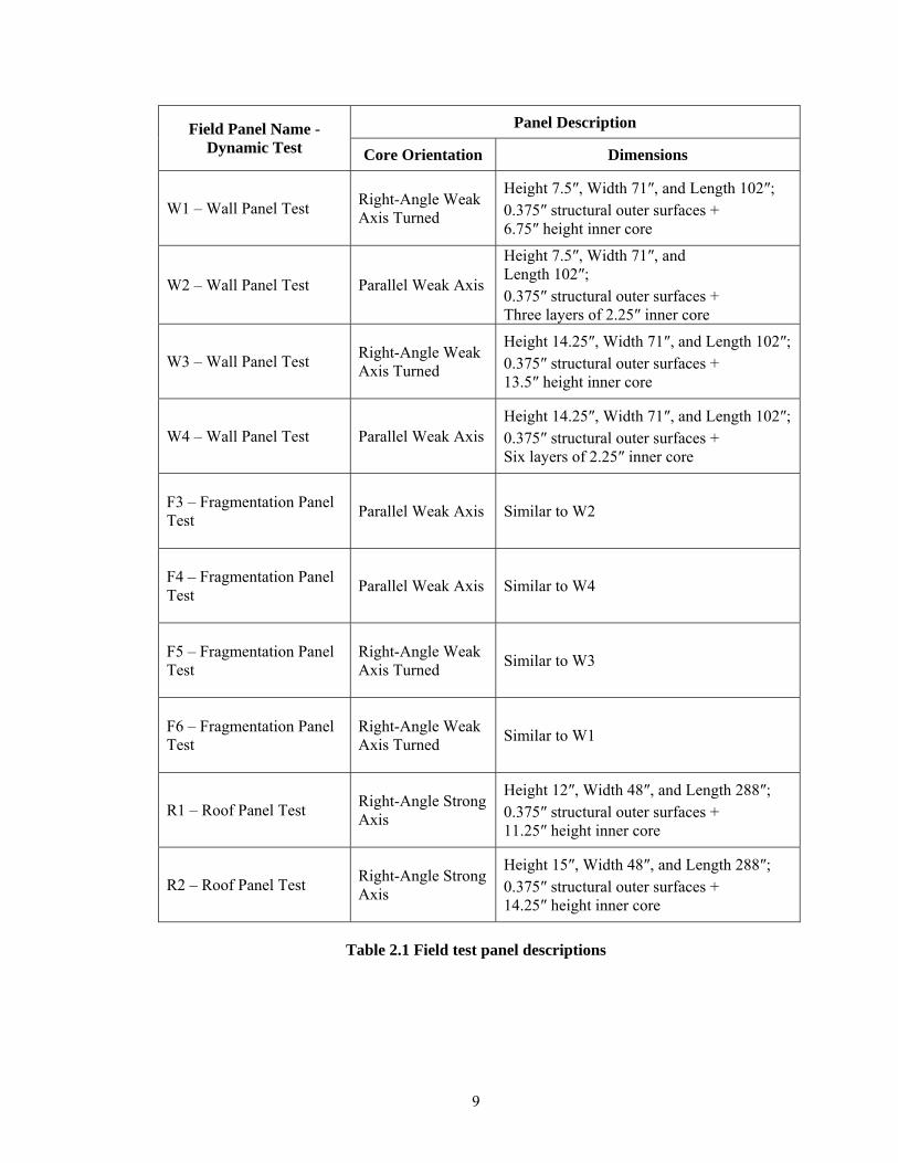
sections, different strengths and properties of the honeycomb panels can be achieved. Listed in
Table 2.1 are the names and details on the honeycomb FRP panels used for field evaluation
discussed in this thesis.

8
Figure 2.1 Five orientation of scaled testing laboratory panels
(e)
(c)
(a) (b)
(d)
9
Panel Description Field Panel Name -Dynamic Test Core Orientation Dimensions
W1 – Wall Panel Test Right-Angle Weak Axis Turned
Height 7.5″, Width 71″, and Length 102″;
0.375″ structural outer surfaces + 6.75″ height inner core
W2 – Wall Panel Test Parallel Weak Axis
Height 7.5″, Width 71″, and Length 102″;
0.375″ structural outer surfaces + Three layers of 2.25″ inner core
W3 – Wall Panel Test Right-Angle Weak Axis Turned
Height 14.25″, Width 71″, and Length 102″;
0.375″ structural outer surfaces + 13.5″ height inner core
W4 – Wall Panel Test Parallel Weak Axis Height 14.25″, Width 71″, and Length 102″;
0.375″ structural outer surfaces + Six layers of 2.25″ inner core
F3 – Fragmentation Panel Test Parallel Weak Axis Similar to W2
F4 – Fragmentation Panel Test Parallel Weak Axis Similar to W4
F5 – Fragmentation Panel Test
Right-Angle Weak Axis Turned Similar to W3
F6 – Fragmentation Panel Test
Right-Angle Weak Axis Turned Similar to W1
R1 – Roof Panel Test Right-Angle Strong Axis
Height 12″, Width 48″, and Length 288″;
0.375″ structural outer surfaces + 11.25″ height inner core
R2 – Roof Panel Test Right-Angle Strong Axis
Height 15″, Width 48″, and Length 288″;
0.375″ structural outer surfaces + 14.25″ height inner core
Table 2.1 Field test panel descriptions
10
2.2. Previous Honeycomb Composite FRP Research
This section will be broken into the following summaries to bring the reader up-to-date
on the previous research performed on similar honeycomb composite fiber-reinforced polymers
(FRP) panels and blast applications where composite FRP have been studied. The review will
focus on information with relevance to this studies application.
In searching papers related to honeycomb composite FRP panels for structural
applications, Dr. Jerry Plunkett of Kansas Structural Composites Inc., Russell, Kansas, was
credited for his work on the subject. He unitized the panels in expedient bridge applications
(Plunkett, 1997). Shortly after the publication of Plunketts (1997) work numerous papers appear
on the subject, some introduce methods of how to analysis honeycomb panels to find their
structural properties that would be needed for design. Similar panels to those that will be used in
this study were examined, the studies consisted from properties of the FRP cell walls and face
laminates to the development of equivalent properties for the built-up composite section (Davalos
et al., 2001). The equivalent properties that Davalos et al. (2001) refers to are also known as the
homogenous properties of the honeycomb FRP panels, and it is with the homogenous properties
that overall bridge designs could be developed. These homogenous properties were developed
using a combination of analytical and experimental results. Further research was found on
heterogeneous solutions that resulted in empirical relations in calculating the stiffness properties;
in other words making the relation between each component and its effect on the overall stiffness
(Qiao and Wang, 2005). Note that all three of these papers/reports focused on what this author
refers to in Section 2.1 as the right-angle strong axis for their evaluations, or panel (c) of Figure
2.1.
Although most of the research focused on the elastic range and the right-angle strong axis
configuration of the honeycomb panels for stiffness evaluation and analysis for deflection design
11
of flexural bridge panels; a few papers were found to include the experimental results of the
ultimate behavior of the panels (Kalny et al., 2004; Cole et al., 2006). Though the stiffness and
micro-structure of the honeycomb panels is important, it is only a small portion of what is need
for blast applications. Kalny et al. (2004) showed that the governing mode of failure of the
honeycomb panels was the horizontal shear developed between the bonded interfaces of the
structural layer and core laminates in flexure. Kalny et al. (2004) recommends the application of
wrapping around the panel edges between the structural or face layer and onto the core laminate
to repair the edge damage of the honeycomb panel. The wrapping resulted in an increase
capacity to the honeycomb panels by providing a level of confinement in the inner core and
structural faces. He describes this as a mechanical locking interaction between the core and
structural layer, the result is an increase in the ultimate capacity by 65% before the core
overcomes the locking and the wrapping to fail (Kalny et al., 2004). As stated above if the
hardened core sections were placed on wet structural layers then clamped or pushed into laminate
to insure the bonding contact the results would be indentations in the structural laminate. Process
of failure now becomes the following, panels are loaded to their horizontal shear capacity the
bonds between the core and structural laminates fail, this should have resulted in the core
laminate buckling out of plane, but the panels continue to carry loads due to the wrapping holding
the rough edges of the core in the indentations on the structural layers (Kalny et al., 2004).
This confinement provided by the FRP wraps to hold the panels together has lent itself to
other structural applications. FRP material has been studied in wrapping applications around
concrete columns for increased confinement and ductility in blast events (Malvar et al., 2004).
Other applications of wet lay-up FRP materials have been used and tested for increasing the
ductility of concrete walls (Muszyuski and Purcell, 2003). The increased ductility allows for the
blast energy to be absorbed by the wall-FRP system, and reduced the dynamic transmitted to the

12
rest of the structure (Mays and Smith, 2003). Further discussion of the blast loading,
characteristics, and analysis will follow in the next section.
2.3. Dynamic Loading and Analysis Review
The dynamic loading of a blast differs in characteristics from more traditional dynamic
loads, like a truck load or a piece of vibrating machinery, in that the blast load occurs in an
instance. It is a high pressure and short duration load whereas a truck loading might spread up to
minute in duration for a bridge and is analyzed as an equivalent static load. A vibrating dynamic
load would be a constant loading that could exist for years and could be analyzed as a perfectly
defined function. Blast on the other hand is full of assumptions and idealized situations to get to
an identifiable and solvable problem. Because of the assumptions a complex rigorous solution
would not be preferred and analysis is recommended to be done by simplified methods (Biggs,
1964). Therefore, the blast response is modeled using the analytical single-degree of freedom
(SDOF) model which has been practiced for years in blast design (Biggs, 1964; Mays and Smith,
2003).
The nature of the blast load application is the amount of energy that is passed from the
explosion to the structure in question. The explosions energy is passed as a shockwave to
structure, where the shockwave can be defined as pressure wave traveling faster than the speed of
sound. The explosives are thought to be instantaneously switched form a solid or liquid to a gas
state creating a hemispherical burst of high pressure that three dimensionally expands to form the
shockwave. The shock decays as a function of the distance way from the explosion. The loading
shape is a triangular free field pressure time history that can be measure at any distance from the
explosion (Figure 2.2).

13
Time
Pres
sure
Positive Duration
Negative Duration
Area under curve = impulse
Peak Pressure
AmbientAir Pressure
Figure 2.2 Ideal blast loading
The integration of the pressure vs. time curve for the positive phase acts as the available
energy or impulse that can be imparted at that time on the structure. The negative phase is
formed by the drag pressures sweeping in behind the positive phase that can impart negative
impulse on the structure. As the shockwave travels and encounters an above ground structure the
leading edge of the wave strikes the structure it is reflected back and amplified by the continued
bombardment of high pressure, this is called the reflected pressure. This high pressure continues
until the positive pressure bleeds around the edges of the structures face or the negative phase
appears and relieves the pressure. The reflected pressure is a function of charge size, standoff
distance, and angle of incident. The angle of incident is the relative angle from the explosives to
the face of the structure in question; the amplified reflected pressure is a factor of this angle. In
the roof applications, which will be discussed in this thesis, the angle of incident goes to zero
leaving the free field pressure to be the blast loading on the roof (TM5-1300, 1990).
14
Both wall and roof applications called for the use of the TM5-1300 (1990) manual for
calculation of the loads for analysis. The manual outlines the simplified procedure for getting an
equivalent triangle loading for design for the roof predictions that can be used in a single-degree
of freedom (SDOF) dynamic modeling procedure for predicting the mid-span deflection.
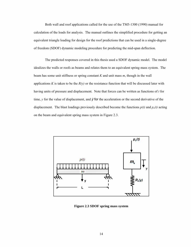
The predicted responses covered in this thesis used a SDOF dynamic model. The model
idealizes the walls or roofs as beams and relates them to an equivalent spring mass system. The
beam has some unit stiffness or spring constant K and unit mass m, though in the wall
applications K is taken to be the R(y) or the resistance function that will be discussed later with
having units of pressure and displacement. Note that forces can be written as functions of t for
time, y for the value of displacement, and ÿ for the acceleration or the second derivative of the
displacement. The blast loadings previously described become the functions p(t) and pe(t) acting
on the beam and equivalent spring mass system in Figure 2.3.
Fe
M
y
k
m
p(t)
L
y
Figure 2.3 SDOF spring mass system
15
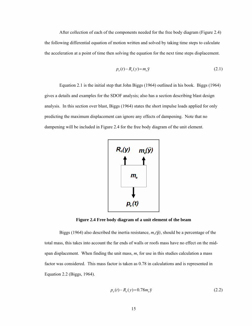
After collection of each of the components needed for the free body diagram (Figure 2.4)
the following differential equation of motion written and solved by taking time steps to calculate
the acceleration at a point of time then solving the equation for the next time steps displacement.
ÿ)()( eee myRtp =− (2.1)
Equation 2.1 is the initial step that John Biggs (1964) outlined in his book. Biggs (1964)
gives a details and examples for the SDOF analysis; also has a section describing blast design
analysis. In this section over blast, Biggs (1964) states the short impulse loads applied for only
predicting the maximum displacement can ignore any effects of dampening. Note that no
dampening will be included in Figure 2.4 for the free body diagram of the unit element.
Figure 2.4 Free body diagram of a unit element of the beam
Biggs (1964) also described the inertia resistance, me(ÿ), should be a percentage of the
total mass, this takes into account the far ends of walls or roofs mass have no effect on the mid-
span displacement. When finding the unit mass, m, for use in this studies calculation a mass
factor was considered. This mass factor is taken as 0.78 in calculations and is represented in
Equation 2.2 (Biggs, 1964).
ÿ78.0)()( eee myRtp =− (2.2)

16
Equation 2.2 will be applied in Chapter 4 in predicting the dynamic response of the
honeycomb FRP panels for designing the tests. Now the laboratory testing and the discussion on
the resistance functions, Re(y), will be presented in the following chapter.
17
3. Static Laboratory Testing and Resistance Functions
A series of static tests were conducted in the laboratory to generate the properties
necessary for evaluating the panels and to be able to develop analytical prediction models. The
laboratory testing consisted initially of small-scale honeycomb FRP panels, which will be
discussed first. In Section 3.2, a procedure for extrapolating the laboratory resistance functions
into the full-scale resistance functions for use in the field wall panel test. A procedure for using
direct methods of laboratory evaluation to retrieve the resistance function for the roof panels will
be discussed in Section 3.3.
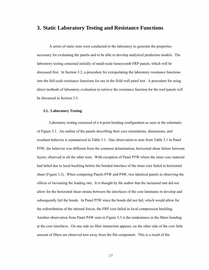
3.1. Laboratory Testing
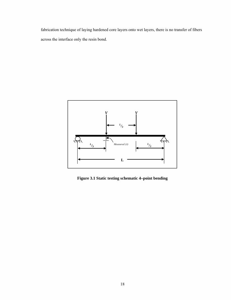
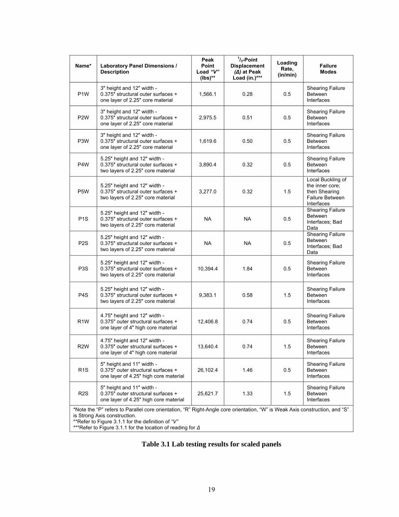
Laboratory testing consisted of a 4-point bending configuration as seen in the schematic
of Figure 3.1. An outline of the panels describing their core orientations, dimensions, and
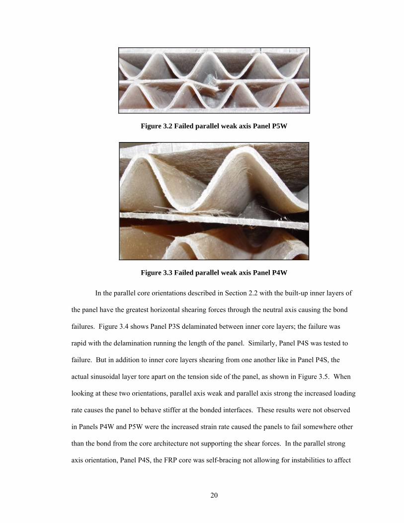
resultant behavior is summarized in Table 3.1. One observation to note from Table 3.1 in Panel
P5W; the behavior was different from the common delamination, horizontal shear failure between
layers, observed in all the other tests. With exception of Panel P5W where the inner core material
had failed due to local buckling before the bonded interface of the inner core failed in horizontal
shear (Figure 3.2). When comparing Panels P5W and P4W, two identical panels in observing the
effects of increasing the loading rate. It is thought by the author that the increased rate did not
allow for the horizontal shear strains between the interfaces of the core laminates to develop and
subsequently fail the bonds. In Panel P5W since the bonds did not fail, which would allow for
the redistribution of the internal forces, the FRP core failed in local compression buckling.
Another observation from Panel P4W seen in Figure 3.3 is the randomness in the fibers bonding
at the core interfaces. On one side no fiber interaction appears, on the other side of the core little
amount of fibers are observed torn away from the flat component. This is a result of the
18
fabrication technique of laying hardened core layers onto wet layers, there is no transfer of fibers
across the interface only the resin bond.
Figure 3.1 Static testing schematic 4–point bending
L
L/3
L/3
V V
L/3 Measured (∆)
19
Name*
Laboratory Panel Dimensions / Description
Peak Point
Load “V” (lbs)**
1/3-Point Displacement
(∆) at Peak Load (in.)***
Loading Rate,
(in/min) Failure Modes
P1W 3″ height and 12″ width - 0.375″ structural outer surfaces + one layer of 2.25″ core material
1,566.1 0.28 0.5 Shearing Failure Between Interfaces
P2W 3″ height and 12″ width - 0.375″ structural outer surfaces + one layer of 2.25″ core material
2,975.5 0.51 0.5 Shearing Failure Between Interfaces
P3W 3″ height and 12″ width - 0.375″ structural outer surfaces + one layer of 2.25″ core material
1,619.6 0.50 0.5 Shearing Failure Between Interfaces
P4W 5.25″ height and 12″ width - 0.375″ structural outer surfaces + two layers of 2.25″ core material
3,890.4 0.32 0.5 Shearing Failure Between Interfaces
P5W 5.25″ height and 12″ width - 0.375″ structural outer surfaces + two layers of 2.25″ core material
3,277.0 0.32 1.5
Local Buckling of the inner core; then Shearing Failure Between Interfaces
P1S 5.25″ height and 12″ width - 0.375″ structural outer surfaces + two layers of 2.25″ core material
NA NA 0.5
Shearing Failure Between Interfaces; Bad Data
P2S 5.25″ height and 12″ width - 0.375″ structural outer surfaces + two layers of 2.25″ core material
NA NA 0.5
Shearing Failure Between Interfaces; Bad Data
P3S 5.25″ height and 12″ width - 0.375″ structural outer surfaces + two layers of 2.25″ core material
10,394.4 1.84 0.5 Shearing Failure Between Interfaces
P4S 5.25″ height and 12″ width - 0.375″ structural outer surfaces + two layers of 2.25″ core material
9,383.1 0.58 1.5 Shearing Failure Between Interfaces
R1W 4.75″ height and 12″ width - 0.375″ outer structural surfaces + one layer of 4″ high core material
12,406.8 0.74 0.5 Shearing Failure Between Interfaces
R2W 4.75″ height and 12″ width - 0.375″ outer structural surfaces + one layer of 4″ high core material
13,640.4 0.74 1.5 Shearing Failure Between Interfaces
R1S 5″ height and 11″ width - 0.375″ outer structural surfaces + one layer of 4.25″ high core material
26,102.4 1.46 0.5 Shearing Failure Between Interfaces
R2S 5″ height and 11″ width - 0.375″ outer structural surfaces + one layer of 4.25″ high core material
25,621.7 1.33 1.5 Shearing Failure Between Interfaces
*Note the “P” refers to Parallel core orientation, “R” Right-Angle core orientation, “W” is Weak Axis construction, and “S” is Strong Axis construction. **Refer to Figure 3.1.1 for the definition of “V” ***Refer to Figure 3.1.1 for the location of reading for ∆
Table 3.1 Lab testing results for scaled panels
20
Figure 3.2 Failed parallel weak axis Panel P5W
Figure 3.3 Failed parallel weak axis Panel P4W
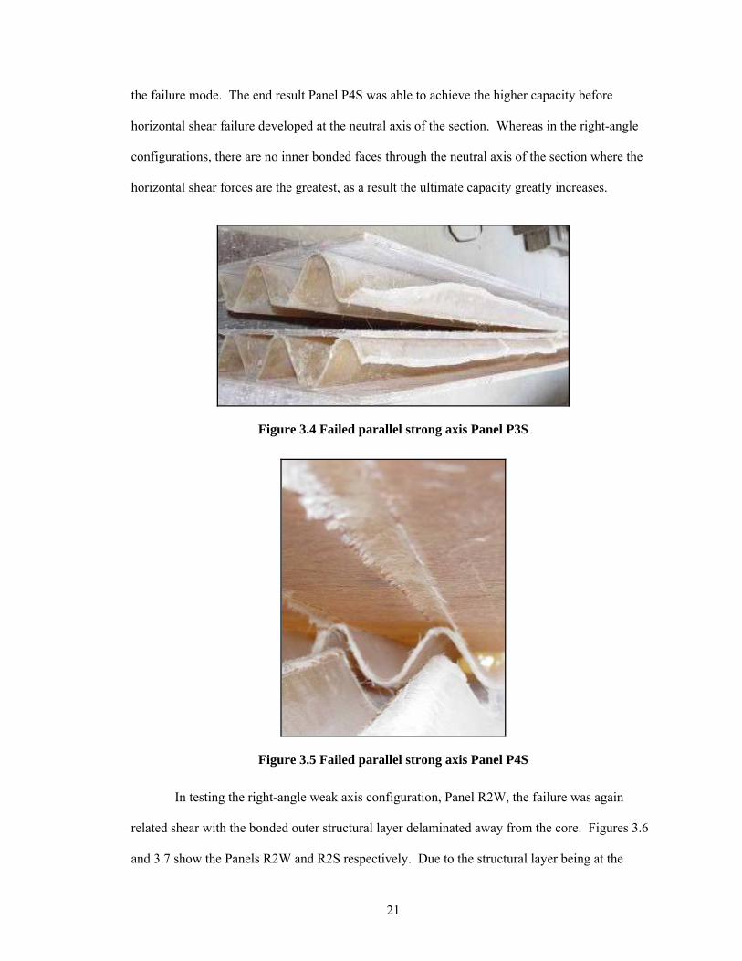
In the parallel core orientations described in Section 2.2 with the built-up inner layers of
the panel have the greatest horizontal shearing forces through the neutral axis causing the bond
failures. Figure 3.4 shows Panel P3S delaminated between inner core layers; the failure was
rapid with the delamination running the length of the panel. Similarly, Panel P4S was tested to
failure. But in addition to inner core layers shearing from one another like in Panel P4S, the
actual sinusoidal layer tore apart on the tension side of the panel, as shown in Figure 3.5. When
looking at these two orientations, parallel axis weak and parallel axis strong the increased loading
rate causes the panel to behave stiffer at the bonded interfaces. These results were not observed
in Panels P4W and P5W were the increased strain rate caused the panels to fail somewhere other
than the bond from the core architecture not supporting the shear forces. In the parallel strong
axis orientation, Panel P4S, the FRP core was self-bracing not allowing for instabilities to affect
21
the failure mode. The end result Panel P4S was able to achieve the higher capacity before
horizontal shear failure developed at the neutral axis of the section. Whereas in the right-angle
configurations, there are no inner bonded faces through the neutral axis of the section where the
horizontal shear forces are the greatest, as a result the ultimate capacity greatly increases.
Figure 3.4 Failed parallel strong axis Panel P3S
Figure 3.5 Failed parallel strong axis Panel P4S
In testing the right-angle weak axis configuration, Panel R2W, the failure was again
related shear with the bonded outer structural layer delaminated away from the core. Figures 3.6
and 3.7 show the Panels R2W and R2S respectively. Due to the structural layer being at the
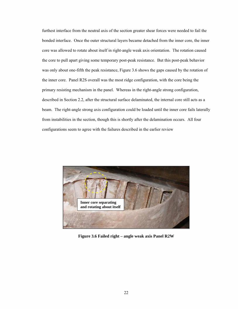
22
furthest interface from the neutral axis of the section greater shear forces were needed to fail the
bonded interface. Once the outer structural layers became detached from the inner core, the inner
core was allowed to rotate about itself in right-angle weak axis orientation. The rotation caused
the core to pull apart giving some temporary post-peak resistance. But this post-peak behavior
was only about one-fifth the peak resistance, Figure 3.6 shows the gaps caused by the rotation of
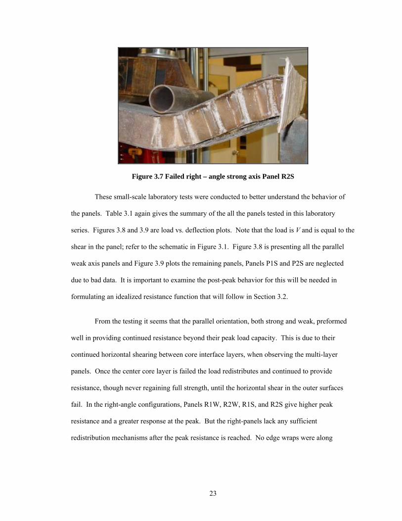
the inner core. Panel R2S overall was the most ridge configuration, with the core being the
primary resisting mechanism in the panel. Whereas in the right-angle strong configuration,
described in Section 2.2, after the structural surface delaminated, the internal core still acts as a
beam. The right-angle strong axis configuration could be loaded until the inner core fails laterally
from instabilities in the section, though this is shortly after the delamination occurs. All four
configurations seem to agree with the failures described in the earlier review
Figure 3.6 Failed right – angle weak axis Panel R2W
Inner core separating and rotating about itself
23
Figure 3.7 Failed right – angle strong axis Panel R2S
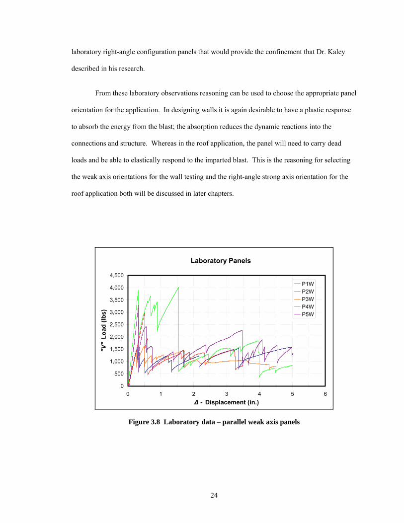
These small-scale laboratory tests were conducted to better understand the behavior of
the panels. Table 3.1 again gives the summary of the all the panels tested in this laboratory
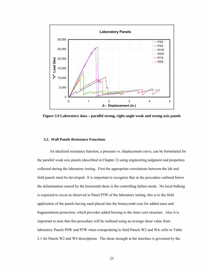
series. Figures 3.8 and 3.9 are load vs. deflection plots. Note that the load is V and is equal to the
shear in the panel; refer to the schematic in Figure 3.1. Figure 3.8 is presenting all the parallel
weak axis panels and Figure 3.9 plots the remaining panels, Panels P1S and P2S are neglected
due to bad data. It is important to examine the post-peak behavior for this will be needed in
formulating an idealized resistance function that will follow in Section 3.2.
From the testing it seems that the parallel orientation, both strong and weak, preformed
well in providing continued resistance beyond their peak load capacity. This is due to their
continued horizontal shearing between core interface layers, when observing the multi-layer
panels. Once the center core layer is failed the load redistributes and continued to provide
resistance, though never regaining full strength, until the horizontal shear in the outer surfaces
fail. In the right-angle configurations, Panels R1W, R2W, R1S, and R2S give higher peak
resistance and a greater response at the peak. But the right-panels lack any sufficient
redistribution mechanisms after the peak resistance is reached. No edge wraps were along
24
laboratory right-angle configuration panels that would provide the confinement that Dr. Kaley
described in his research.
From these laboratory observations reasoning can be used to choose the appropriate panel
orientation for the application. In designing walls it is again desirable to have a plastic response
to absorb the energy from the blast; the absorption reduces the dynamic reactions into the
connections and structure. Whereas in the roof application, the panel will need to carry dead
loads and be able to elastically respond to the imparted blast. This is the reasoning for selecting
the weak axis orientations for the wall testing and the right-angle strong axis orientation for the
roof application both will be discussed in later chapters.
Laboratory Panels
0
500
1,000
1,500
2,000
2,500
3,000
3,500
4,000
4,500
0 1 2 3 4 5 6∆ - Displacement (in.)
"V"
Load
(lbs
)
P1WP2WP3WP4WP5W
Figure 3.8 Laboratory data – parallel weak axis panels
25
Laboratory Panels
0
5,000
10,000
15,000
20,000
25,000
30,000
0 1 2 3 4 5∆ - Displacement (in.)
"V"
Load
(lbs
)
P3SP4SR1WR2WR1SR2S
Figure 3.9 Laboratory data – parallel strong, right-angle weak and strong axis panels
3.2. Wall Panels Resistance Functions
An idealized resistance function, a pressure vs. displacement curve, can be formulated for
the parallel weak axis panels (described in Chapter 2) using engineering judgment and properties
collected during the laboratory testing. First the appropriate correlations between the lab and
field panels must be developed. It is important to recognize that in the procedure outlined below
the delamination caused by the horizontal shear is the controlling failure mode. No local bulking
is expected to occur as observed in Panel P5W of the laboratory testing, this is to the field
application of the panels having sand placed into the honeycomb core for added mass and
fragmentation protection, which provides added bracing to the inner core structure. Also it is
important to note that this procedure will be outlined using an average shear value from
laboratory Panels P4W and P5W when extrapolating to field Panels W2 and W4, refer to Table
2.1 for Panels W2 and W4 descriptions. The shear strength at the interface is governed by the
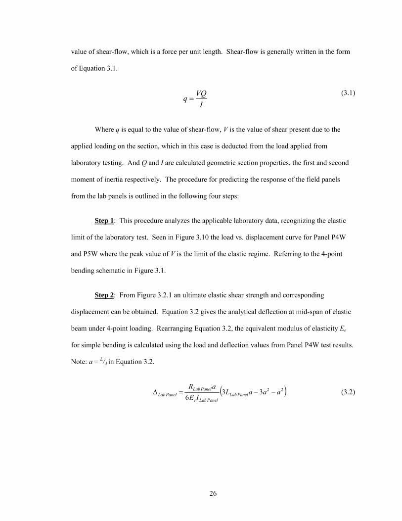
26
value of shear-flow, which is a force per unit length. Shear-flow is generally written in the form
of Equation 3.1.
IVQq =
(3.1)
Where q is equal to the value of shear-flow, V is the value of shear present due to the
applied loading on the section, which in this case is deducted from the load applied from
laboratory testing. And Q and I are calculated geometric section properties, the first and second
moment of inertia respectively. The procedure for predicting the response of the field panels
from the lab panels is outlined in the following four steps:
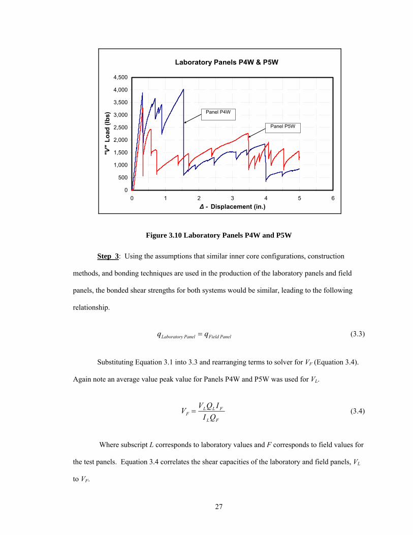
Step 1: This procedure analyzes the applicable laboratory data, recognizing the elastic
limit of the laboratory test. Seen in Figure 3.10 the load vs. displacement curve for Panel P4W
and P5W where the peak value of V is the limit of the elastic regime. Referring to the 4-point
bending schematic in Figure 3.1.
Step 2: From Figure 3.2.1 an ultimate elastic shear strength and corresponding
displacement can be obtained. Equation 3.2 gives the analytical deflection at mid-span of elastic
beam under 4-point loading. Rearranging Equation 3.2, the equivalent modulus of elasticity Ee
for simple bending is calculated using the load and deflection values from Panel P4W test results.
Note: a = L/3 in Equation 3.2.
( )22336
aaaLIE
aRPanelLab
PanelLabe
PanelLabPanelLab −−=∆ (3.2)
27
Laboratory Panels P4W & P5W
0
500
1,000
1,500
2,000
2,500
3,000
3,500
4,000
4,500
0 1 2 3 4 5 6∆ - Displacement (in.)
"V"
Load
(lbs
) Panel P4W
Panel P5W
Figure 3.10 Laboratory Panels P4W and P5W
Step 3: Using the assumptions that similar inner core configurations, construction
methods, and bonding techniques are used in the production of the laboratory panels and field
panels, the bonded shear strengths for both systems would be similar, leading to the following
relationship.
PanelFieldPanelLaboratory qq = (3.3)
Substituting Equation 3.1 into 3.3 and rearranging terms to solver for VF (Equation 3.4).
Again note an average value peak value for Panels P4W and P5W was used for VL.
FL
FLLF QI
IQVV = (3.4)
Where subscript L corresponds to laboratory values and F corresponds to field values for
the test panels. Equation 3.4 correlates the shear capacities of the laboratory and field panels, VL
to VF.
28
Step 4: Assuming the horizontal shear causing failure does not depend on the type of
loading, the maximum shear under 4-point loading is assumed the same as for uniform loading.
In other words, Vmax4-point ≡ Vmax
uniform, where Vmax is equal to the VF computed from Equation 3.4.
The distributed load, wmax, corresponding to this maximum shear as computed from Equation 3.5.
FLV
w maxmax
2= ; LF = span length of field panels (3.5)
Using wmax from Equation 3.5 and equivalent Ee from Step 2, the load vs. displacement
response at the max point is computed from Equation 3.6:
Fe
F
IELw
3845 4
max=∆ (3.6)
Further reductions can be made to formulate a pressure excreted on the panels using
Equation 3.7.
widthsamplebwp = ; b = width of field panels (3.7)
Therefore, the pressure vs. deflection (static resistance function) is computed from
Equation 3.8.
max38445 pIEbL
Fe
F⎟⎟⎠
⎞⎜⎜⎝
⎛=∆ (3.8)
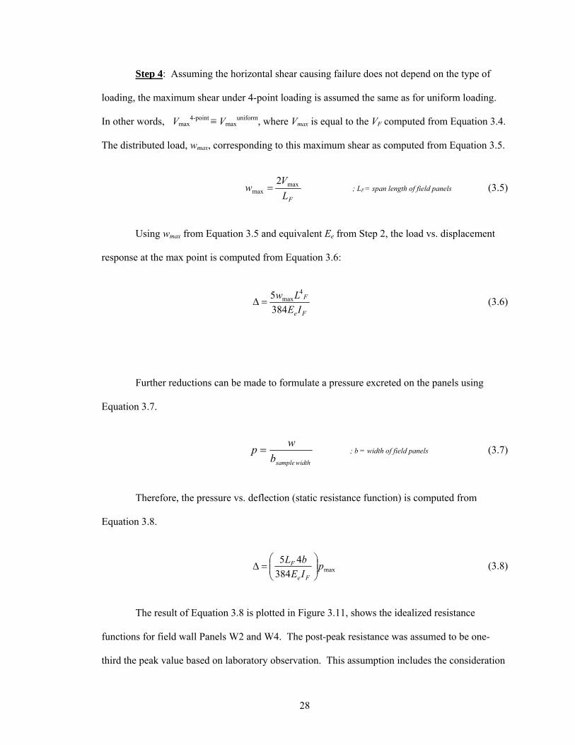
The result of Equation 3.8 is plotted in Figure 3.11, shows the idealized resistance
functions for field wall Panels W2 and W4. The post-peak resistance was assumed to be one-
third the peak value based on laboratory observation. This assumption includes the consideration
29
of residual resistance from the continued shearing of the outer layers and structural surface, which
will be re-examined using field response under blast loading in Chapter 5 of this thesis.
Idealized Resistance Functions
0
2
4
6
8
10
12
14
16
18
0 2 4 6 8 10 12 14
∆ - Displacement (in.)
Pres
sure
(psi
)
Panel W2Panel W4
Figure 3.11 Idealized resistance function
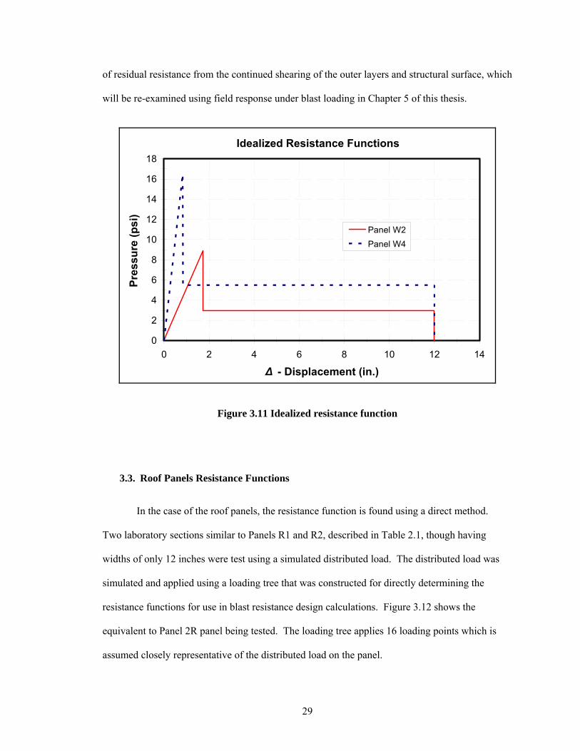
3.3. Roof Panels Resistance Functions
In the case of the roof panels, the resistance function is found using a direct method.
Two laboratory sections similar to Panels R1 and R2, described in Table 2.1, though having
widths of only 12 inches were test using a simulated distributed load. The distributed load was
simulated and applied using a loading tree that was constructed for directly determining the
resistance functions for use in blast resistance design calculations. Figure 3.12 shows the
equivalent to Panel 2R panel being tested. The loading tree applies 16 loading points which is
assumed closely representative of the distributed load on the panel.

30
In application the roof panel is required to remain elastic during the blast loading. Thus
in the static testing, no post-peak behavior was needed to be collected as was done with small-
scale wall panels. In testing the 12 inch width equivalent section panels, both their resistance
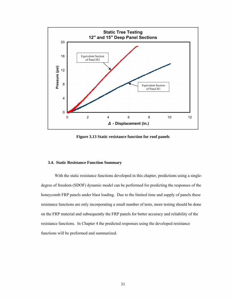
functions were linear, see Figure 3.13, though the laboratory equivalent to Panel 2R was not taken
to failure. The failure mode seen in the laboratory equivalent of Panel 1R was similar to that seen
in Panels R1S and R2S of the scaled testing, Section 3.1, which were controlled by the internal
core delaminating away from the outer structural surface allowing the core to torsionally-buckle
in the complete loose of capacity.
Figure 3.12 16–point loading tree
31
Static Tree Testing12″ and 15″ Deep Panel Sections
0
4
8
12
16
20
0 2 4 6 8 10 12
∆ - Displacement (in.)
Pres
sure
(psi
)
Figure 3.13 Static resistance function for roof panels
3.4. Static Resistance Function Summary
With the static resistance functions developed in this chapter, predictions using a single-
degree of freedom (SDOF) dynamic model can be performed for predicting the responses of the
honeycomb FRP panels under blast loading. Due to the limited time and supply of panels these
resistance functions are only incorporating a small number of tests, more testing should be done
on the FRP material and subsequently the FRP panels for better accuracy and reliability of the
resistance functions. In Chapter 4 the predicted responses using the developed resistance
functions will be preformed and summarized.
Equivalent Section of Panel R1
Equivalent Section of Panel R2
32
4. Dynamic Response Predictions Under Blast Loadings
The resistance functions developed in Chapter 3 for the wall panels and roof panels were
combined with dynamic modeling procedure for Section 2.3 to produce the following dynamic
response predictions are the honeycomb FRP panels under the blast loading. The resistance
function of any panel can be incorporated into a single-degree of freedom (SDOF) dynamic
model to predict the mid-span displacement at any time step during the blast event. First the
prediction for the wall panels will be presented followed by the roof panels.
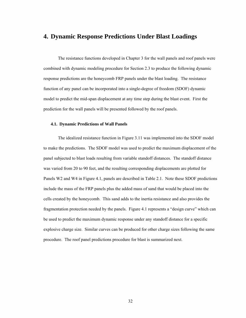
4.1. Dynamic Predictions of Wall Panels
The idealized resistance function in Figure 3.11 was implemented into the SDOF model
to make the predictions. The SDOF model was used to predict the maximum displacement of the
panel subjected to blast loads resulting from variable standoff distances. The standoff distance
was varied from 20 to 90 feet, and the resulting corresponding displacements are plotted for
Panels W2 and W4 in Figure 4.1, panels are described in Table 2.1. Note these SDOF predictions
include the mass of the FRP panels plus the added mass of sand that would be placed into the
cells created by the honeycomb. This sand adds to the inertia resistance and also provides the
fragmentation protection needed by the panels. Figure 4.1 represents a “design curve” which can
be used to predict the maximum dynamic response under any standoff distance for a specific
explosive charge size. Similar curves can be produced for other charge sizes following the same
procedure. The roof panel predictions procedure for blast is summarized next.
33
Standoff Design Curve For Panels W2 and W4
Charge Size of (Weight Omitted) (Flake TNT)
20
30
40
50
60
70
80
90
0 4 8 12 16∆ - Displacement (in.)
Stan
doff
(ft)
Panel W2 SDOFPanel W4 SDOF
Figure 4.1 Design curve for field Panel W2 and W4
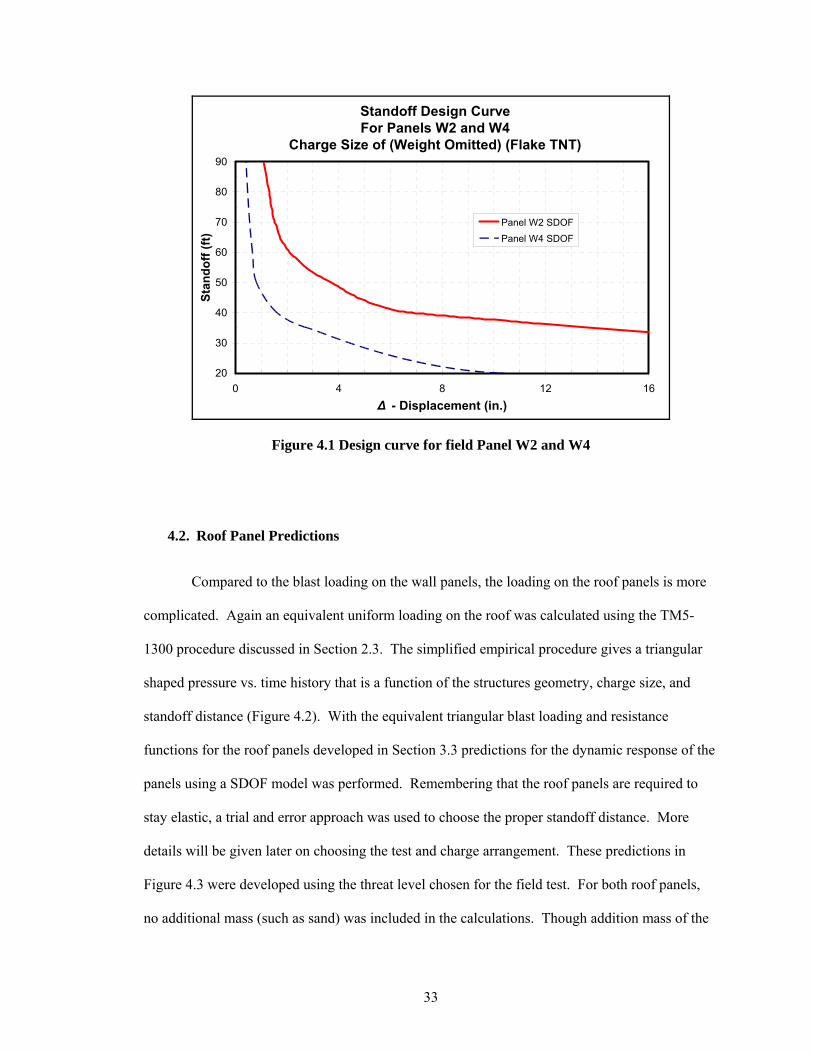
4.2. Roof Panel Predictions
Compared to the blast loading on the wall panels, the loading on the roof panels is more
complicated. Again an equivalent uniform loading on the roof was calculated using the TM5-
1300 procedure discussed in Section 2.3. The simplified empirical procedure gives a triangular
shaped pressure vs. time history that is a function of the structures geometry, charge size, and
standoff distance (Figure 4.2). With the equivalent triangular blast loading and resistance
functions for the roof panels developed in Section 3.3 predictions for the dynamic response of the
panels using a SDOF model was performed. Remembering that the roof panels are required to
stay elastic, a trial and error approach was used to choose the proper standoff distance. More
details will be given later on choosing the test and charge arrangement. These predictions in
Figure 4.3 were developed using the threat level chosen for the field test. For both roof panels,
no additional mass (such as sand) was included in the calculations. Though addition mass of the
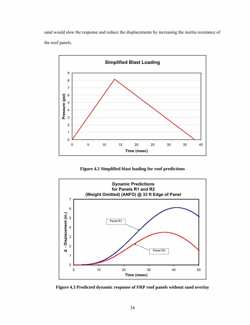
34
sand would slow the response and reduce the displacements by increasing the inertia resistance of
the roof panels.
Simplified Blast Loading
0
1
2
3
4
5
6
7
8
9
0 5 10 15 20 25 30 35 40
Time (msec)
Pres
sure
(psi
)
Figure 4.2 Simplified blast loading for roof predictions
Dynamic Predictionsfor Panels R1 and R2
(Weight Omitted) (ANFO) @ 33 ft Edge of Panel
0
1
2
3
4
5
6
7
0 10 20 30 40 50Time (msec)
∆ -
Dis
plac
emen
t (in
.)
Panel R1
Panel R2
Figure 4.3 Predicted dynamic response of FRP roof panels without sand overlay

35
4.3. Prediction Summary
The analytical prediction models for the wall panels developed in this chapter were
verified using live explosives in the recommend field tests. Field setup test results will be
provided in Chapters 5 for the FRP wall panels and Chapter 7 for the FRP roof panels. Though
all the predictions used loadings formulated by the empirical procedure in the TM5-1300, actual
loads will be measured experimentally during the testing to verify the predicted loadings.
Chapter 5 will follow with the summarization of the wall panel testing and discussion of the
accuracy of the predictions.
36
5. Field Evaluation of FRP Wall Panels Subjected to Blast
The analytical prediction models developed in Chapters 3 and 4 are verified
experimentally in this chapter. A field experiment using live explosives was conducted on
honeycomb FRP wall panels with the assistance of Air Force Research Laboratory, Tyndall Air
Force Base, FL. The field testing consists of a blast evaluation of the FRP wall panels in flexure.
All testing results will be presented.
5.1. Field Test Setup
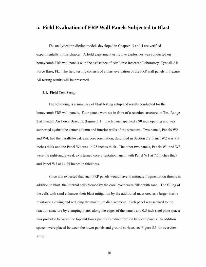
The following is a summary of blast testing setup and results conducted for the
honeycomb FRP wall panels. Four panels were set in front of a reaction structure on Test Range
2 at Tyndall Air Force Base, FL (Figure 5.1). Each panel spanned a 90 inch opening and was
supported against the center column and interior walls of the structure. Two panels, Panels W2
and W4, had the parallel-weak axis core orientation, described in Section 2.2, Panel W2 was 7.5
inches thick and the Panel W4 was 14.25 inches thick. The other two panels, Panels W1 and W3,
were the right-angle weak axis turned core orientation, again with Panel W1 at 7.5 inches thick
and Panel W3 at 14.25 inches in thickness.
Since it is expected that such FRP panels would have to mitigate fragmentation threats in
addition to blast, the internal cells formed by the core layers were filled with sand. The filling of
the cells with sand enhances their blast mitigation by the additional mass creates a larger inertia
resistance slowing and reducing the maximum displacement. Each panel was secured to the
reaction structure by clamping plates along the edges of the panels and 0.5 inch steel plate spacer
was provided between the top and lower panels to reduce friction between panels. In addition
spacers were placed between the lower panels and ground surface, see Figure 5.1 for overview
setup.
37
Figure 5.1 Wall panel – setup
To determine the threat level the wall panels were thought to be used in a temporary
checkpoint scenario. In this situation, the panels would be supported against a reaction frame or
other panels to form an enclosure similar to concept presented in Figure 1.1. An attacker could
approach the checkpoint and detonate their explosives in close proximity. The panels would need
to protect soldiers occupying the checkpoint. For this test, the charge was selected to be (Weight
Omitted from this thesis) of TNT.
Assumptions for what would limit the performance of the panels in this setup are needed
to set boundary conditions in designing optimum test setup. The slipping between the panels and
the center column would be the controlling limit on the maximum displacement that the panels
could undergo. Assuming a parabolic deflected shape, the maximum allowable slip between the
column and panel is 6 inches. The corresponding maximum mid-span displacement would be 12
W1
W3
W2
W4
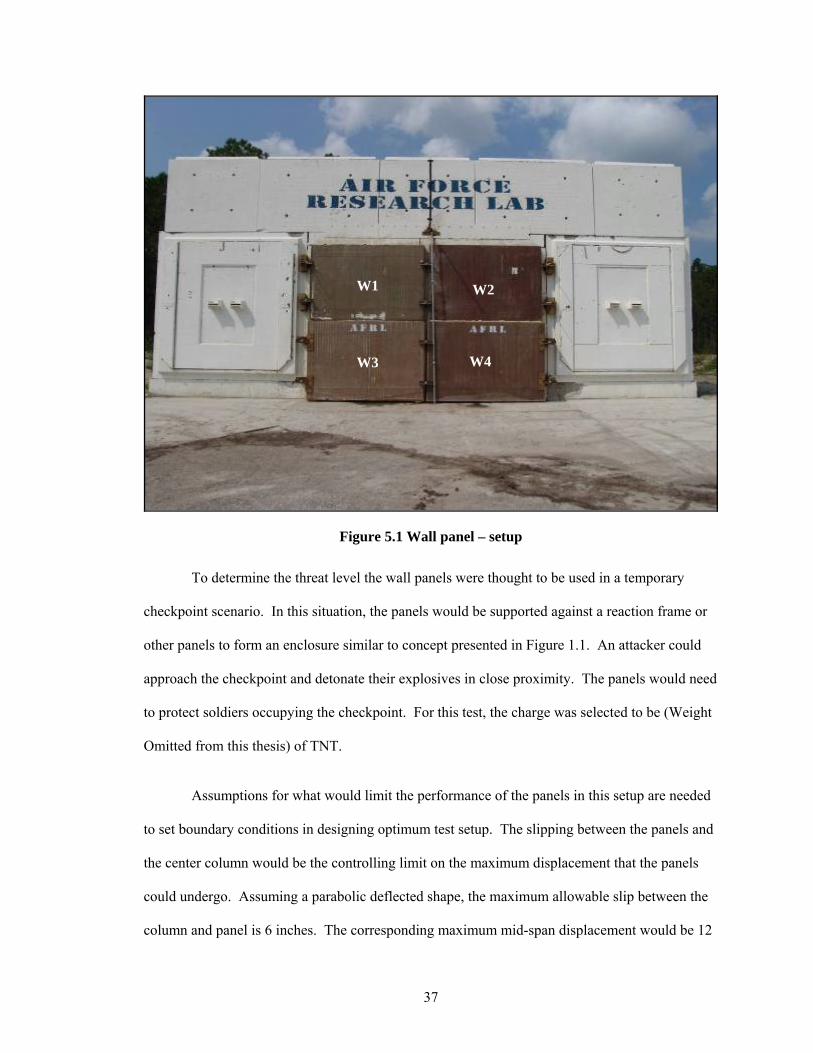
38
inches in a parabolic deflected shape. Using the design chart of Figure 4.1, a vertical line can be
drawn at 12 inches displacement for which the corresponding lower-bound standoff for wall
Panel W2 becomes 35 feet (Figure 5.2).
Standoff Design CurveFor Panels W2 and W4
Charge Size of (Weight Omitted) (Flake TNT)
20
30
40
50
60
70
80
90
0 4 8 12 16∆ - Displacement (in.)
Stan
doff
(ft)
Panel W2 SDOFPanel W4 SDOF
Figure 5.2 Standoff design curve
5.2. Field Test Results and Verification
Again, the field experiment was designed based on these threat level parameters of
(Weight Omitted) of TNT at 35 feet. The center of explosive charge was placed 6 feet above
ground level, see Figure 5.3. Mid-span displacement of all four panels was recorded during test,
as well as the external reflected pressure and free-field pressure readings, results will be covered
later in this chapter. Post-test observations indicate that the panels preformed as it was predicted
in Chapter 3 of this thesis. Panels delaminated, with the outer surfaces saperating from the cores.
In Panel W2 and W4 the internal core layers were seperated from each other. In Panel W1 the
39
core sections were pulled from one another and the structural surface was completely debonded.
But in Panel W3 only small amounts of damage were seen.
Figures 5.4 through 5.9 give more details on the observed damages. Lower panels,
Panels W3 and W4, rebounded outward breaking the clamping anchorage, and as a result upper
panels, Panels W1 and W2, fell due to lack of support beneath them, see Figure 5.4. Panel W2
was delaminated between all layers as shown in Figure 5.5. This could be attributed to the weak
connection between core layers and face sheets. Figure 5.6 shows little amounts of fiber bonding
present between layers, which limits the horizontal shear transfer between layers and
subsequently reduces the capacity of the FRP panels. Similar delamination of outer structural
layers from the core was also observed in Panel W1, indicated in Figure 5.7 and 5.8 with the
outer structural layer completely separated from the core. The core in Panel W1 also showed
signs of being ripped away from itself similar to the behavior of the laboratory Panels R1W and
R2W, described in Section 3.1. Also note in Figure 5.8 bonding between the structural surface
and the core was sufficient to tear away fibers from the structural surface. Figure 5.9 shows an
indention were Panel W3 had rested against the reaction structure. This indicates that large shear
forces (or dynamic reactions) were experienced in Panel W3 during the blast event. This further
indicates the statement that Panels W1 and W3 can be related in some degree to laboratory Panels
R1W and R2W in behavior, laboratory Panels R1W and R2W developed larger reaction forces
resulting in higher peak resistance. It is believed that Panel W3 remained in its elastic regime
during the testing. In the same manor Panel W1 was past its elastic regime and consequently
destroyed all of its resistance.
40
Figure 5.3 Wall panel – pretest
Figure 5.4 Post-test view of panels
3355--fftt SSttaannddooffff
FFllaakkee TTNNTT
66--fftt ttoo CCeenntteerr

41
Figure 5.5 Post-test Panel W2
Figure 5.6 Post-test view of Panel W2
Little fiber bonding between layers.
Delamination of layers
42
Figure 5.7 Post-test view of Panel W1
Figure 5.8 Post-test view of Panel W1
Improved bonding to outer surfaces, but little to no bonding between core sections layers.
43
Figure 5.9 Post-test view of Panel W3
For additional evaluation and analytical predictions, the pressure-time histories as well as
the displacement gauge readings were needed. Figure 5.10 shows a schematic of the test setup
with the various gauges and locations used to monitor the blast environment and responses of the
wall panels during the test. Four reflected pressure gauges R1, R2, R3, and R4 were used plus
one free-field pressure gauge FF1. Reflected pressure gauge R3 recorded bad data and its results
are omitted from this thesis. Four displacement gauges D1, D2, D3, and D4 were used to
measure the mid-point response of Panels W1, W2, W3, and W4, respectively. Table 5.1
provides a summary of the results from each of gauges used. The impulse is calculated by
integrating the pressure-time history, and represents a measure of the energy imparted into the
wall panels as a result of the blast.
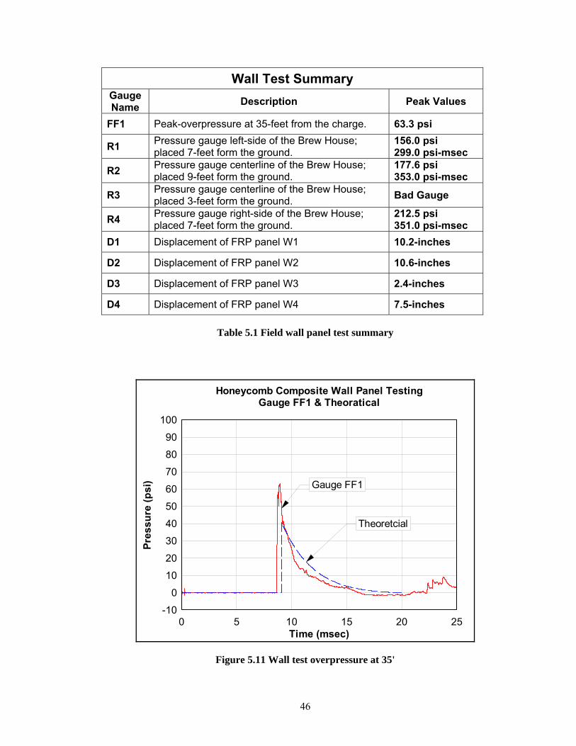
The result of free field gauge FF1 were used to verify that the detonation of the charge
was effective by comparing the FF1 reading to pressure prediction calculated by the TM5-1300
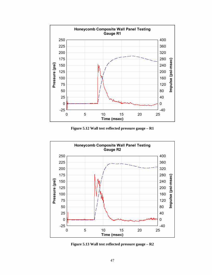
procedure, see Figure 5.11. Figures 5.12 through 5.14 show the pressure-time history of the
reflect pressure gauges and the corresponding reflected impulse for each gauge. Figure 5.15
through 5.18 show the mid-span displacement response of the FRP wall panels during the blast
event. The maximum displacement in the wall panels of 10.6 inches was recorded by gauge D2
Location of the support, the indentation indicates beings shear failure in the core.

44
in Panel W2, where the least displacement of 2.4 inches was recorded by gauge D3 in Panel W3.
As stated earlier it is believed that Panel W3 deflected within its elastic regime leaving the panel
with very little damage, and thus the flexural integrity was mostly maintained. This resulted in
most of the stored energy during positive deformation was recovered during the rebound phase,
which created negative reactions too large for the side anchors to withstand.
The measured response of Panels W2 and W4 was used to verify the analytical prediction
developed in Chapter 4. For Panel W2, the predicted dynamic response was 12 inches which was
relatively similar to the measured response of 10.6 inches. Similarly, the predicted response of
Panel W4 was 2.8 inches and the actual measurement was 7.5 inches. In the instance of W4 the
idealized resistance function was not accurate of the real panel. In extrapolating data from
laboratory Panels P4W and P5W, both two layer panels, then scaling the data to Panels W2 and
W4 the accuracy is reduced when increasing the number of laminated core layers in the panel for
making an estimate on the residual resistance in the post-peak behavior. If the residual resistance
in the resistance functions in Figure 3.11 of Section 3.2 were reduced for Panel W4 to 1 psi, then
using in the SDOF model to predict the corresponding maximum displacement, the result would
be 11.1 inches. Furthermore if the residual resistance was 2 psi the resultant displacement would
be 6.2 inches. It will be stated in the conclusion that accuracy will come with testing full-scale
wall panels in the lab to be able record the actual post-peak resistance, similar to the laboratory
testing of the roof panels. In general, the predicted response is higher than the measured
response, which is conservative that can be attributed to the dynamic increases in the panels that
were not considered in the analytical predictions.
45
Figure 5.10 Wall test schematic
Displacement Gauges
Free Field Pressure Gauges
Reflected Pressure Gauges
FF1
D1 D4
D2
D3
R2
R1
R4
R3
35-ft Standoff
35-ft Standoff
6-ft to center
46
Wall Test Summary Gauge Name Description Peak Values
FF1 Peak-overpressure at 35-feet from the charge. 63.3 psi
R1 Pressure gauge left-side of the Brew House; placed 7-feet form the ground.
156.0 psi 299.0 psi-msec
R2 Pressure gauge centerline of the Brew House; placed 9-feet form the ground.
177.6 psi 353.0 psi-msec
R3 Pressure gauge centerline of the Brew House; placed 3-feet form the ground. Bad Gauge
R4 Pressure gauge right-side of the Brew House; placed 7-feet form the ground.
212.5 psi 351.0 psi-msec
D1 Displacement of FRP panel W1 10.2-inches
D2 Displacement of FRP panel W2 10.6-inches
D3 Displacement of FRP panel W3 2.4-inches
D4 Displacement of FRP panel W4 7.5-inches
Table 5.1 Field wall panel test summary
Time (msec)
Pres
sure
(psi
)
Honeycomb Composite Wall Panel TestingGauge FF1 & Theoratical
0 5 10 15 20 25-10
0
10
20
30
40
50
60
70
80
90
100
Theoretcial
Gauge FF1
Figure 5.11 Wall test overpressure at 35'
47
Time (msec)
Pres
sure
(psi
)
Impu
lse
(psi
-mse
c)
Honeycomb Composite Wall Panel TestingGauge R1
0 5 10 15 20 25-25 -40
0 0
25 40
50 80
75 120
100 160
125 200
150 240
175 280
200 320
225 360
250 400
Figure 5.12 Wall test reflected pressure gauge – R1
Time (msec)
Pres
sure
(psi
)
Impu
lse
(psi
-mse
c)
Honeycomb Composite Wall Panel TestingGauge R2
0 5 10 15 20 25-25 -40
0 0
25 40
50 80
75 120
100 160
125 200
150 240
175 280
200 320
225 360
250 400
Figure 5.13 Wall test reflected pressure gauge – R2
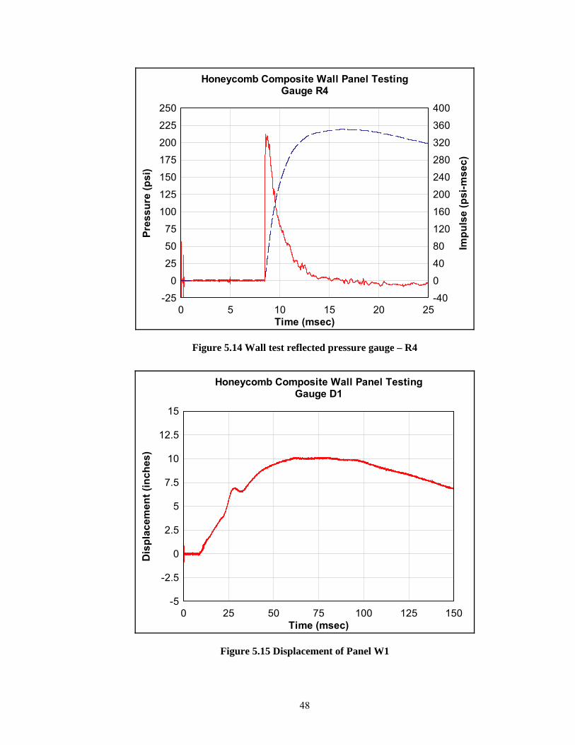
48
Time (msec)
Pres
sure
(psi
)
Impu
lse
(psi
-mse
c)
Honeycomb Composite Wall Panel TestingGauge R4
0 5 10 15 20 25-25 -40
0 0
25 40
50 80
75 120
100 160
125 200
150 240
175 280
200 320
225 360
250 400
Figure 5.14 Wall test reflected pressure gauge – R4
Time (msec)
Dis
plac
emen
t (in
ches
)
Honeycomb Composite Wall Panel TestingGauge D1
0 25 50 75 100 125 150-5
-2.5
0
2.5
5
7.5
10
12.5
15
Figure 5.15 Displacement of Panel W1
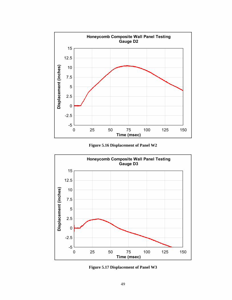
49
Time (msec)
Dis
plac
emen
t (in
ches
)
Honeycomb Composite Wall Panel TestingGauge D2
0 25 50 75 100 125 150-5
-2.5
0
2.5
5
7.5
10
12.5
15
Figure 5.16 Displacement of Panel W2
Time (msec)
Dis
plac
emen
t (in
ches
)
Honeycomb Composite Wall Panel TestingGauge D3
0 25 50 75 100 125 150-5
-2.5
0
2.5
5
7.5
10
12.5
15
Figure 5.17 Displacement of Panel W3
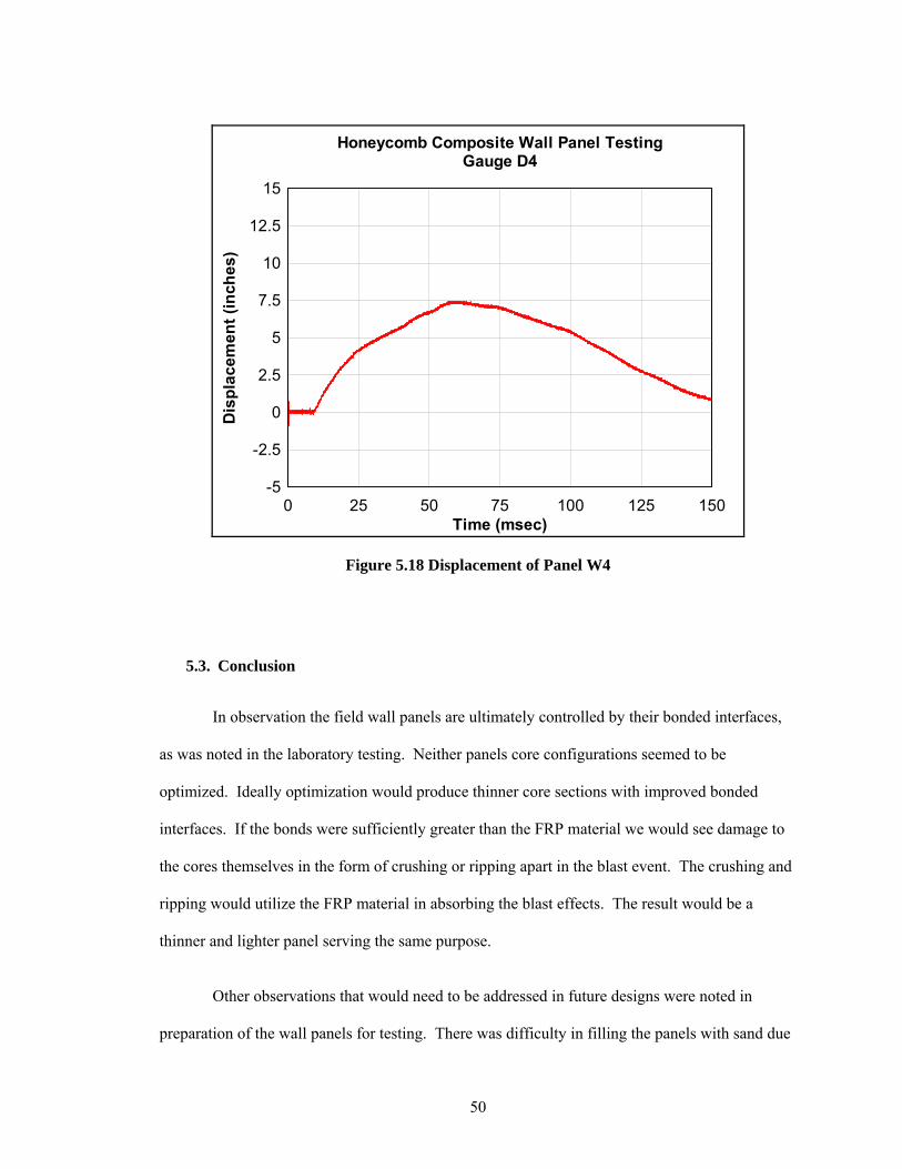
50
Time (msec)
Dis
plac
emen
t (in
ches
)
Honeycomb Composite Wall Panel TestingGauge D4
0 25 50 75 100 125 150-5
-2.5
0
2.5
5
7.5
10
12.5
15
Figure 5.18 Displacement of Panel W4
5.3. Conclusion
In observation the field wall panels are ultimately controlled by their bonded interfaces,
as was noted in the laboratory testing. Neither panels core configurations seemed to be
optimized. Ideally optimization would produce thinner core sections with improved bonded
interfaces. If the bonds were sufficiently greater than the FRP material we would see damage to
the cores themselves in the form of crushing or ripping apart in the blast event. The crushing and
ripping would utilize the FRP material in absorbing the blast effects. The result would be a
thinner and lighter panel serving the same purpose.
Other observations that would need to be addressed in future designs were noted in
preparation of the wall panels for testing. There was difficulty in filling the panels with sand due

51
to stray fibers in the honeycomb core continuously plugged with sand. The stray fibers are a
result of the fabrication methods, again in the hand lay-up the side in non-contact with the mold
does not have a gel coat to provide the smooth finish. So a method was devised to wash to sand
into the core; holes were drilled into the bottom of the panel to drain the excess water out of the
panels. Ideally fine graded sand could be used in filling the panels but due to the cost of graded
sand in-situ materials were used.
Although more laboratory and field testing would be ideal in developing a better
understanding of these panels in order to make adequate designs for temporary structures. It
would also be beneficial to have full-scale wall panels tested in the laboratory to directly
determine their resistance functions and better understand their post-peak resistance if any. The
extrapolated residual behavior of the panels, did not accurately predict the actual behavior. The
accuracy of predicting the residual behavior only worsened when increasing the overall thickness
of the panels. More conclusions will be added at the end of Chapter 6 about the wall panels after
the discussion of the fragmentation testing of similar panels.
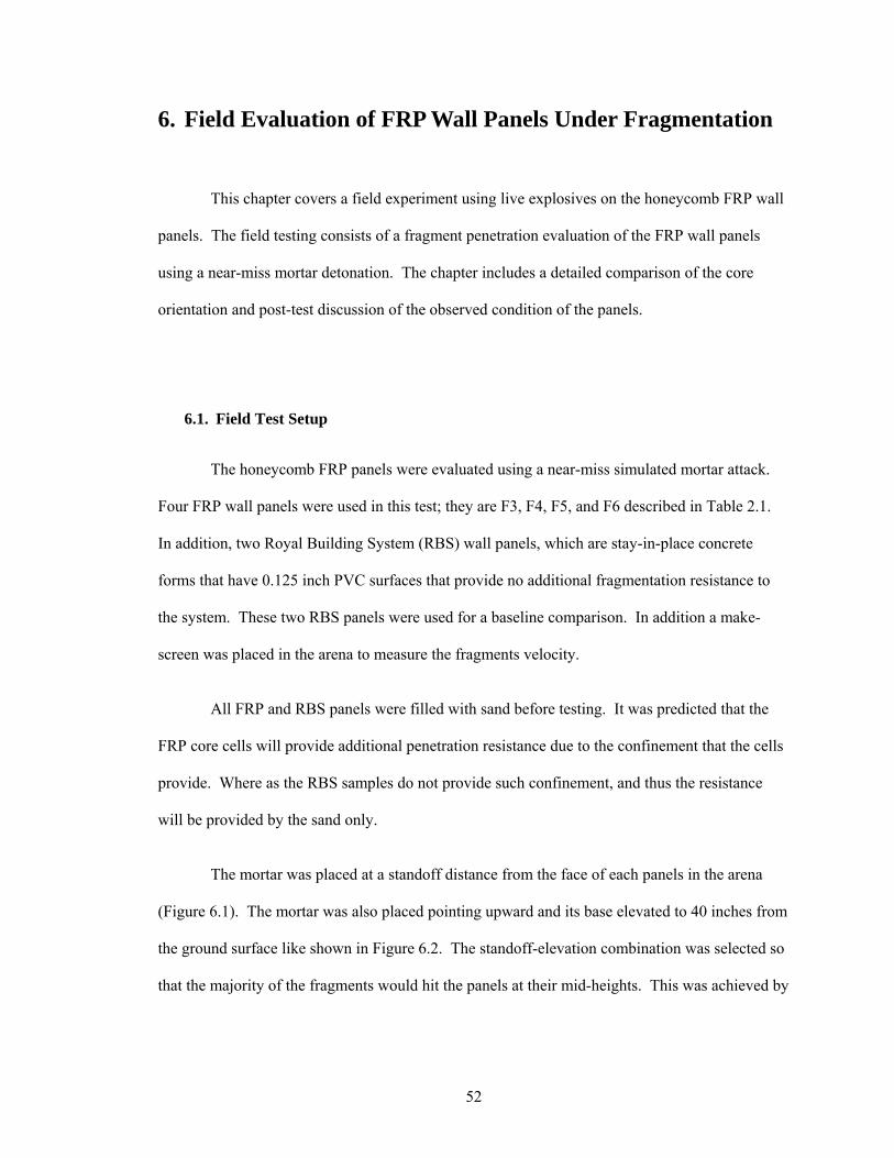
52
6. Field Evaluation of FRP Wall Panels Under Fragmentation
This chapter covers a field experiment using live explosives on the honeycomb FRP wall
panels. The field testing consists of a fragment penetration evaluation of the FRP wall panels
using a near-miss mortar detonation. The chapter includes a detailed comparison of the core
orientation and post-test discussion of the observed condition of the panels.
6.1. Field Test Setup
The honeycomb FRP panels were evaluated using a near-miss simulated mortar attack.
Four FRP wall panels were used in this test; they are F3, F4, F5, and F6 described in Table 2.1.
In addition, two Royal Building System (RBS) wall panels, which are stay-in-place concrete
forms that have 0.125 inch PVC surfaces that provide no additional fragmentation resistance to
the system. These two RBS panels were used for a baseline comparison. In addition a make-
screen was placed in the arena to measure the fragments velocity.
All FRP and RBS panels were filled with sand before testing. It was predicted that the
FRP core cells will provide additional penetration resistance due to the confinement that the cells
provide. Where as the RBS samples do not provide such confinement, and thus the resistance
will be provided by the sand only.
The mortar was placed at a standoff distance from the face of each panels in the arena
(Figure 6.1). The mortar was also placed pointing upward and its base elevated to 40 inches from
the ground surface like shown in Figure 6.2. The standoff-elevation combination was selected so
that the majority of the fragments would hit the panels at their mid-heights. This was achieved by
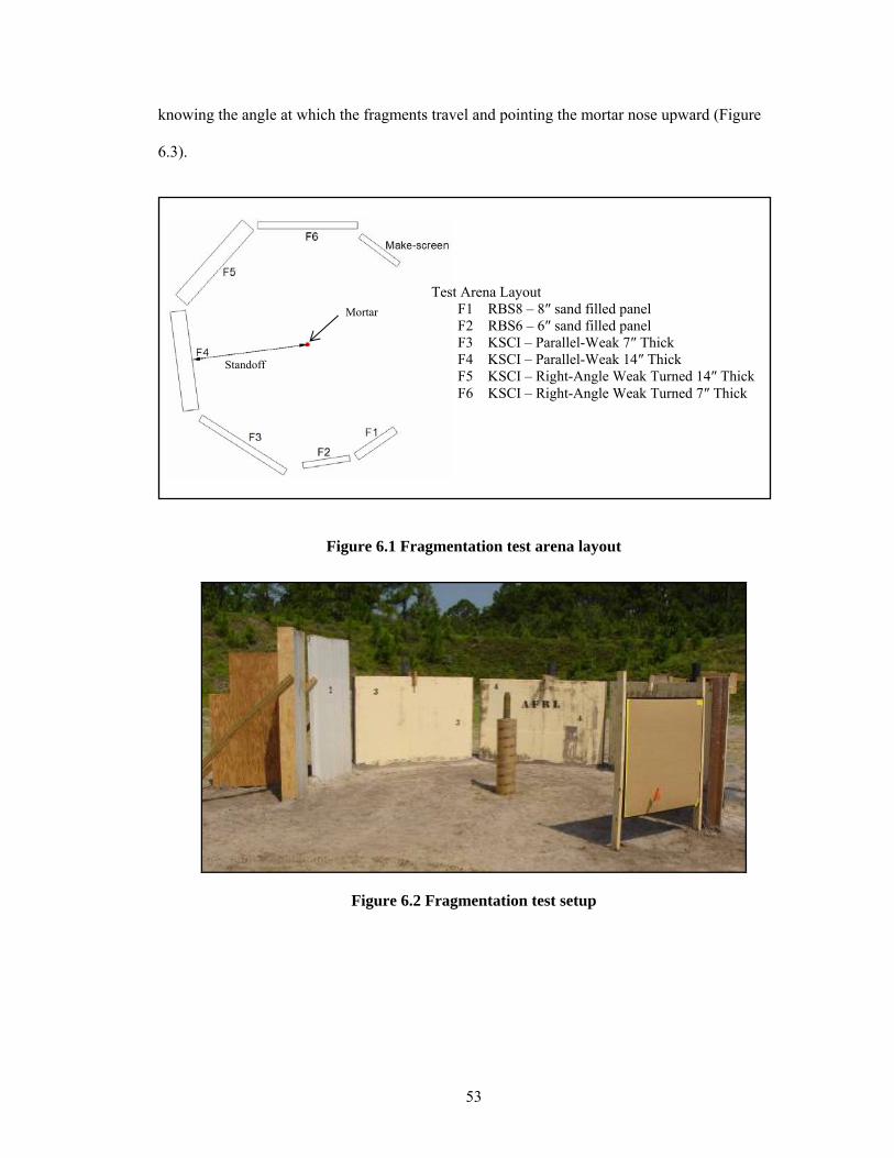
53
knowing the angle at which the fragments travel and pointing the mortar nose upward (Figure
6.3).
Figure 6.1 Fragmentation test arena layout
Figure 6.2 Fragmentation test setup
Standoff
Mortar
Test Arena Layout F1 RBS8 – 8″ sand filled panel F2 RBS6 – 6″ sand filled panel F3 KSCI – Parallel-Weak 7″ Thick F4 KSCI – Parallel-Weak 14″ Thick F5 KSCI – Right-Angle Weak Turned 14″ Thick F6 KSCI – Right-Angle Weak Turned 7″ Thick
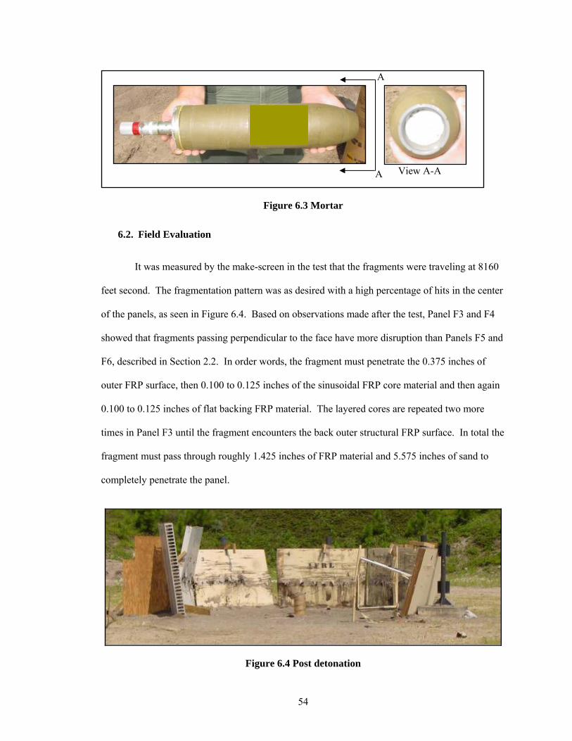
54
Figure 6.3 Mortar
6.2. Field Evaluation
It was measured by the make-screen in the test that the fragments were traveling at 8160
feet second. The fragmentation pattern was as desired with a high percentage of hits in the center
of the panels, as seen in Figure 6.4. Based on observations made after the test, Panel F3 and F4
showed that fragments passing perpendicular to the face have more disruption than Panels F5 and
F6, described in Section 2.2. In order words, the fragment must penetrate the 0.375 inches of
outer FRP surface, then 0.100 to 0.125 inches of the sinusoidal FRP core material and then again
0.100 to 0.125 inches of flat backing FRP material. The layered cores are repeated two more
times in Panel F3 until the fragment encounters the back outer structural FRP surface. In total the
fragment must pass through roughly 1.425 inches of FRP material and 5.575 inches of sand to
completely penetrate the panel.
Figure 6.4 Post detonation
A
A
View A-A

55
Seen in Figure 6.5 is the post-detonation view of Panel F3, were large amounts of
damage at the edges of the panels were fragments needed to penetrate less sand as a result
gapping holes were observed. Also the blast from the mortar was enough to tip the panel back
into the metal stand. Panels F4 and F5 similar fragmentation pattern was observed though less
hits near the edges; both Panels F4 and F5 were standing vertical after the detonation (Figures 6.6
and 6.7). Figure 6.8 shows Panel F6 where again like Panel F3 was tipped back by the blast
pressure and momentum of the fragments.
Figure 6.5 Post-test Panel F3
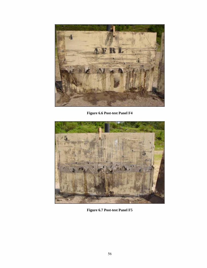
56
Figure 6.6 Post-test Panel F4
Figure 6.7 Post-test Panel F5
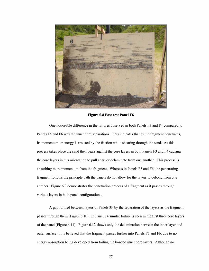
57
Figure 6.8 Post-test Panel F6
One noticeable difference in the failures observed in both Panels F3 and F4 compared to
Panels F5 and F6 was the inner core separations. This indicates that as the fragment penetrates,
its momentum or energy is resisted by the friction while shearing through the sand. As this
process takes place the sand then bears against the core layers in both Panels F3 and F4 causing
the core layers in this orientation to pull apart or delaminate from one another. This process is
absorbing more momentum from the fragment. Whereas in Panels F5 and F6, the penetrating
fragment follows the principle path the panels do not allow for the layers to debond from one
another. Figure 6.9 demonstrates the penetration process of a fragment as it passes through
various layers in both panel configurations.
A gap formed between layers of Panels 3F by the separation of the layers as the fragment
passes through them (Figure 6.10). In Panel F4 similar failure is seen in the first three core layers
of the panel (Figure 6.11). Figure 6.12 shows only the delamination between the inner layer and
outer surface. It is believed that the fragment passes further into Panels F5 and F6, due to no
energy absorption being developed from failing the bonded inner core layers. Although no
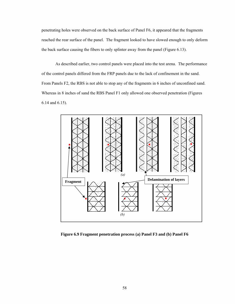
58
penetrating holes were observed on the back surface of Panel F6, it appeared that the fragments
reached the rear surface of the panel. The fragment looked to have slowed enough to only deform
the back surface causing the fibers to only splinter away from the panel (Figure 6.13).
As described earlier, two control panels were placed into the test arena. The performance
of the control panels differed from the FRP panels due to the lack of confinement in the sand.
From Panels F2, the RBS is not able to stop any of the fragments in 6 inches of unconfined sand.
Whereas in 8 inches of sand the RBS Panel F1 only allowed one observed penetration (Figures
6.14 and 6.15).
Figure 6.9 Fragment penetration process (a) Panel F3 and (b) Panel F6
Delamination of layers Fragment
(a)
(b)
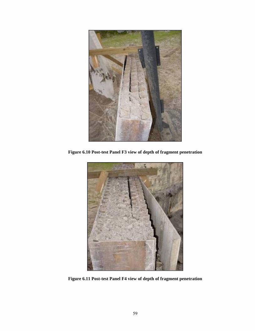
59
Figure 6.10 Post-test Panel F3 view of depth of fragment penetration
Figure 6.11 Post-test Panel F4 view of depth of fragment penetration
60
Figure 6.12 Post-test Panel F5 view of depth of fragment penetration

61
Figure 6.13 Post-test Panel F6 view of depth of fragment penetration
62
Figure 6.14 Front face of Panels F1 and F2 (RBS)
Figure 6.15 Rear faces of Panels F1 and F2
63
6.3. Conclusion
The honeycomb FRP wall panels used for this series of testing completed their goal of
stopping all the fragments. Although one draw back that needs to be evaluated would be the
health concerns; once the panel is struck with fragments they have large amounts of fibers that fill
the air and spread into the surrounding vicinity. The breathing hazard associated with the FRP
panels post-attack should be evaluated. An estimate on what is an allowable exposure to the
airborne FRP material should be assessed. Further work is still needed to perform a cost analysis
comparing alternative and existing materials that can be used in fragment protection. It is
suggested that a comparison between theses honeycomb FRP panels and conventional sand bags
be compared for levels of fragmentation protection.
Overall the honeycomb FRP wall panels performed less desirable in both scenarios of
blast and fragmentation mitigation. When the FRP panels are used as a blast mitigation measure
they provide energy absorption but it is at a low utilization of FRP materials for the level of
protection that it provides. As stated in Section 5.3, the FRP panels should be optimized to
become a more viable option in the blast mitigation. As a fragmentation mitigation measure the
FRP panels are effective but to what level are the benefits of using the FRP panels over another
product which is less hazardous after an attack and can serve similar purposes. The honeycomb
FRP has potential for other applications in structures that will be more suited for their behavior
characteristics. These other applications will be discussed next in the roof panel chapter.
64
7. Roof Blast Panel Testing
The analytical prediction model developed in Chapters 3 and 4 were used to design the
field test for the roof panels under blast. The field test results were used to verify the engineering
analysis and design method developed. The experimental test setup and results are presented in
this chapter.
7.1. Roof Blast Test Setup
For this test, the roof panels were placed on rigid concrete blocks along their short
dimension. In an actual field scenario, it is expected that sand bags will be placed on top of the
roof panels to protect against a direct mortar hit. But in this test, no sand was placed on top of the
roof panels since the FRP panels available for this program were very stiff, and thus the recorded
displacement during testing would have been considered small due to the added mass of the sand
slowing the response and adding increased inertia to the panels. The response would have made
it, hard to verify the analytical model predictions.
In designing the experiment, the location of the explosive charge was considered either at
the end, location A or at the side, location B (Figure 7.1). Since location A produces a complex
blast loading scenario (TM5-1300, 1990), the end-shot blast test was selected for this study.
65
Figure 7.1 Charge placements
The test-range at Tyndall AFB limits the size of the explosives, the threat level was
selected to be (Weight Omitted) of ammonium nitrate and fuel oil (ANFO). The standoff
distance of 30 feet from the face of the support blocks was selected to produce the desired
response of the panels useful for the analytical predictions verifications (Figure 7.2). Finally,
earth berms were placed along the sides of the test setup to prevent the shockwave from loading
the underside of the roof panels, see Figure 7.2 and 7.3. Stud walls were placed along side the
panels to prevent the berms from interfering with the displacement of the panels.
Two FRP roof panels were tested, Panels 1R and 2R. One panel was 12 inches deep,
Panel 1R, and the other 15 inches deep, Panel 2R. Both were made with the right-angle strong
axis orientation, refer back to Figure 2.1 and Table 2.1 presented in Section 2.2. The panels were
designed to deflect a maximum of clear-span-to-deflection ratio of L/180 under a sand overlay of
12 inches. The assumed over lay of sand was an estimate on the depth of sand bags that would be
needed for fragmentation cover on top of the temporary structures.
Side-shot Location B
End-shot Location A
20 ft Clear -span
4 ft width

66
Free field pressure gauges as well as deflection gauges were used to document the
shockwave environment and dynamic response of the panels, respectively (Figure 7.4). The test
results are summarized next.
Figure 7.2 Roof panels – 30 feet standoff to block face
Figure 7.3 Roof panels – end view pretest
30-ft Standoff to block face
33-ft Standoff to panel face
ANFO
67
Figure 7.4 Roof Test Schematic
Displacement Gauges
Free Field Pressure Gauges
FF1
FF7
FF5
FF4
FF3
FF2
FF8
FF6
D1
D4
D2
D5
D3
D6
10-ft
10-ft
35-ft
5-ft
Panel R2
Panel R1
5-ft
5-ft
5-ft
30-ft
5-ft

68
7.2. Roof Testing Results and Evaluation
In viewing the free field pressure gauges results, gauge FF1 compares well to the
theoretical predicted pressure (TM5-1300, 1990). Gauges FF4 and FF7 had small spikes after the
peak pressure (refer to Figures 7.5 through 7.12 and Table 7.1). It is thought that these later
spikes were caused by the shockwave reflecting off the soil berms along side of the panels. The
free field gauges on top of the panels, FF2, FF3, FF5, FF6, and FF8, also have double spikes.
These spikes on the other hand are believed to be caused by the shockwave reaching the gauge
from the hemispherical burst, making the first peak. Then the second spike is believed to be from
the reflected pressure bleeding over the front face of the supporting structure causing higher
overpressures.
The measured field responses of the roof panels tested are shown in Figure 7.13 through
7.18 and are given in Table 7.1. The Maximum field response was recorded at mid-span of each
panel, gauges D3 and D4 for panels 2R and 1R, respectively. The analytical value of 6.1 inches
over predicts the measured response of 3.0 inches for Panel 1R. Similarly the measured field
response of the roof panels indicate that both Panels 1R and 2R behaved stiffer than predicted,
which could be attributed to the following reasons. The field roof panels had edge wrapping
which is a 0.375 inches structural surface; refer to Section 2.2, added to the edges for handling
processes in this case. Another observation from the predicted response to the actual is that the
predicted used the empirical procedure from the TM5-1300 for formulating the loading. This
procedure was originally developed for design processes where over predictions are welcomed in
calculating loading scenarios.
In Panel 2R a larger negative displacement was recorded due to the failure of a tie down
anchor, which allowed the panel to break-free from the supports during the rebound phase of the
response. See Figures 7.13, 7.15, and 7.17.
69
Roof Test Summary Gauge Name Description Peak Values
FF1 Free Field Gauge at 35 feet on the ground 87.7 psi FF2 Free Field Gauge at 35 feet on rooftop 49.3 psi FF3 Free Field Gauge at 40 feet on rooftop 37.6 psi FF4 Free Field Gauge at 45 feet on the ground 47.8 psi FF5 Free Field Gauge at 45 feet on rooftop 37.1 psi FF6 Free Field Gauge at 50 feet on rooftop 33.8 psi FF7 Free Field Gauge at 55 feet on the ground 33.5 psi FF8 Free Field Gauge at 55 feet on rooftop 21.8 psi D1 Displacement at the nearest quarter-point Panel 2R 1.0-inches D2 Displacement at the nearest quarter-point Panel 1R 2.2-inches D3 Displacement at the midpoint Panel 2R 1.8-inches D4 Displacement at the midpoint Panel 1R 3.0-inches D5 Displacement at the furthest quarter-point Panel 2R 1.5-inches D6 Displacement at the furthest quarter-point Panel 1R 2.5-inches
Table 7.1 Field roof panel test summary
Time (msec)
Pres
sure
(psi
)
Honeycomb Composite Roof Panel TestingGauge FF1 & Theoretical
0 5 10 15 20 25 30 35 40-10
0
10
20
30
40
50
60
70
80
90
Theoretical
FF1
Figure 7.5 Free field gauge FF1
70
Time (msec)
Pres
sure
(psi
)
Honeycomb Composite Roof Panel TestingGauge FF2
0 5 10 15 20 25 30 35 40-10
0
10
20
30
40
50
60
70
80
90
Figure 7.6 Free field gauge FF2
Time (msec)
Pres
sure
(psi
)
Honeycomb Composite Roof Panel TestingGauge FF3
0 5 10 15 20 25 30 35 40-10
0
10
20
30
40
50
60
70
80
90
Figure 7.7 Free field gauge FF3
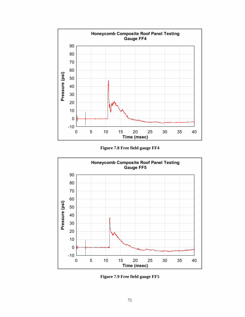
71
Time (msec)
Pres
sure
(psi
)
Honeycomb Composite Roof Panel TestingGauge FF4
0 5 10 15 20 25 30 35 40-10
0
10
20
30
40
50
60
70
80
90
Figure 7.8 Free field gauge FF4
Time (msec)
Pres
sure
(psi
)
Honeycomb Composite Roof Panel TestingGauge FF5
0 5 10 15 20 25 30 35 40-10
0
10
20
30
40
50
60
70
80
90
Figure 7.9 Free field gauge FF5
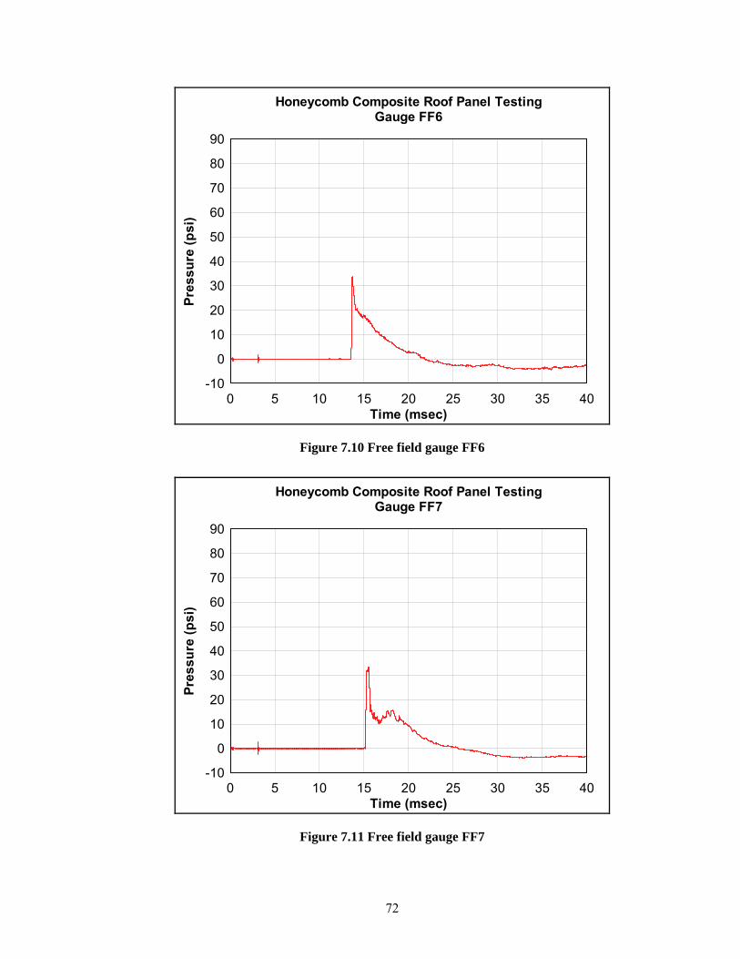
72
Time (msec)
Pres
sure
(psi
)
Honeycomb Composite Roof Panel TestingGauge FF6
0 5 10 15 20 25 30 35 40-10
0
10
20
30
40
50
60
70
80
90
Figure 7.10 Free field gauge FF6
Time (msec)
Pres
sure
(psi
)
Honeycomb Composite Roof Panel TestingGauge FF7
0 5 10 15 20 25 30 35 40-10
0
10
20
30
40
50
60
70
80
90
Figure 7.11 Free field gauge FF7
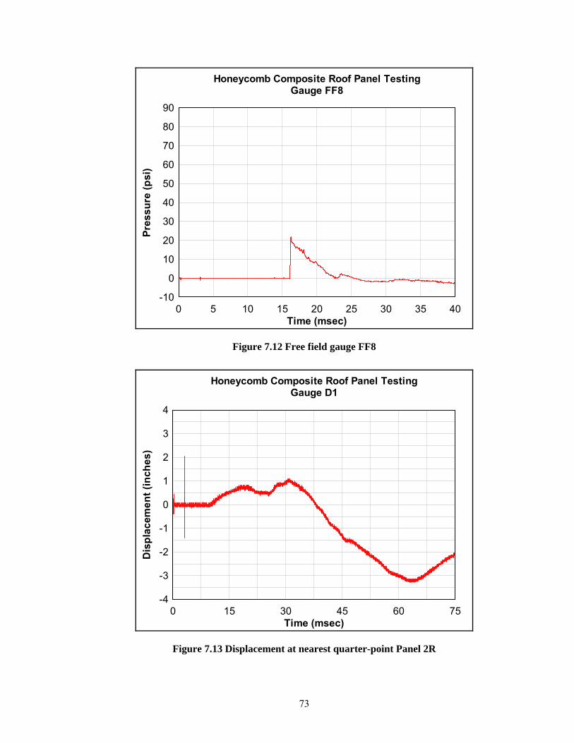
73
Time (msec)
Pres
sure
(psi
)
Honeycomb Composite Roof Panel TestingGauge FF8
0 5 10 15 20 25 30 35 40-10
0
10
20
30
40
50
60
70
80
90
Figure 7.12 Free field gauge FF8
Time (msec)
Dis
plac
emen
t (in
ches
)
Honeycomb Composite Roof Panel TestingGauge D1
0 15 30 45 60 75-4
-3
-2
-1
0
1
2
3
4
Figure 7.13 Displacement at nearest quarter-point Panel 2R
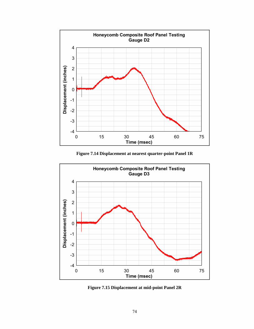
74
Time (msec)
Dis
plac
emen
t (in
ches
)
Honeycomb Composite Roof Panel TestingGauge D2
0 15 30 45 60 75-4
-3
-2
-1
0
1
2
3
4
Figure 7.14 Displacement at nearest quarter-point Panel 1R
Time (msec)
Dis
plac
emen
t (in
ches
)
Honeycomb Composite Roof Panel TestingGauge D3
0 15 30 45 60 75-4
-3
-2
-1
0
1
2
3
4
Figure 7.15 Displacement at mid-point Panel 2R
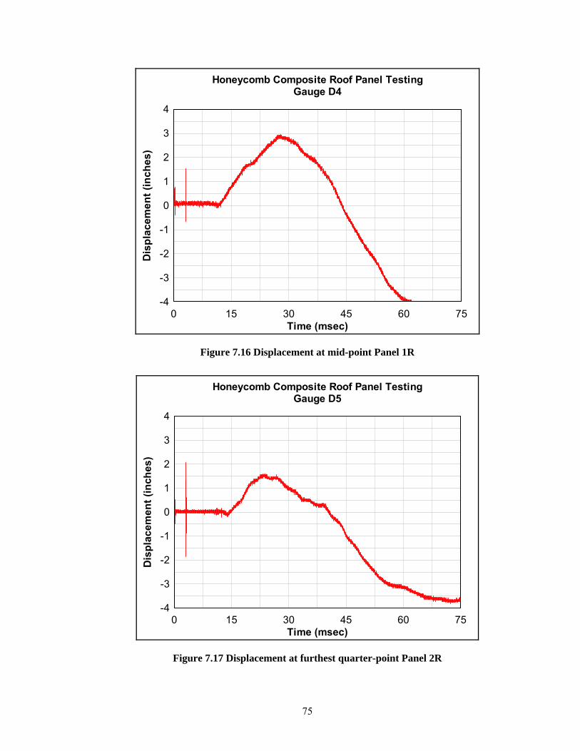
75
Time (msec)
Dis
plac
emen
t (in
ches
)
Honeycomb Composite Roof Panel TestingGauge D4
0 15 30 45 60 75-4
-3
-2
-1
0
1
2
3
4
Figure 7.16 Displacement at mid-point Panel 1R
Time (msec)
Dis
plac
emen
t (in
ches
)
Honeycomb Composite Roof Panel TestingGauge D5
0 15 30 45 60 75-4
-3
-2
-1
0
1
2
3
4
Figure 7.17 Displacement at furthest quarter-point Panel 2R

76
Time (msec)
Dis
plac
emen
t (in
ches
)
Honeycomb Composite Roof Panel TestingGauge D6
0 15 30 45 60 75-4
-3
-2
-1
0
1
2
3
4
Figure 7.18 Displacement at furthest quarter-point Panel 1R
7.3. Roof Test Conclusion
Based on the laboratory and field tests conducted, honeycomb FRP panels performed
more desirably when used in roof applications. Since the panels have a relatively high strength-
to-weight ratio and large observed ductility, they can be considered good candidates for roof
structures. Such panels can be designed to ensure an elastic response during dynamic loading and
have minimum service deflections under dead loads. But additional evaluation is still needed to
optimize the panels design and core architecture. The performance of these roof panels under
long-term sustained sand dead load is still needed. The response of the panels when sand is
placed on top will change; the sand will slow the response under the blast loading and reduce the
total deflection.
The FRP roof panels will need to be designed for tie downs to resist the rebound forces
occurring during post detonation. Thinner roof panels would reduce the stiffness and assist in

77
reducing the loads transmitted to the overall supporting structure, walls or supporting frame. It is
hypothesized that panel depths between 8 inches and 10 inches could be adequate to resist the
dead load and blast threats similar to the ones evaluated in this roof study. Additional laboratory
and field testing will be needed to accurately quantify their blast protection level.
78
8. Conclusions and Recommendations
Honeycomb fiber-reinforced polymers (FRP) panels were evaluated for the Air Force
Research Laboratory (AFRL), Tyndall Air Base, FL to study their feasibility as temporary
structures that could provide protection for blast and fragmentation. The panels were tested in the
laboratory and the recommendations were used to design field experiments. Simulated field
applications using live explosives and munitions were conducted. The following is a bulleted
recap of the work and prudent observations that were made throughout this thesis.
• Laboratory static-testing provided engineering information about the characteristics of
the FRP material and how the construction of the panels influenced the overall behavior.
This information was then used in developing analytical predictions for recommended
design of field experiments.
• Four panels were placed in front of a reaction structure and were submitted to a blast
event. Their dynamic response and pressure vs. time histories were recorded. The
overall performances of the panels were controlled by horizontal shear force that
developed. In other words bonded interfaces of the inner cores failed, leaving the panel
with a very small residual resistance in absorbing the blast load. Therefore, it is believed
that the FRP panels do not meet the optimum performance in blast mitigation as wall
panels. Additional research is still needed to optimize the FRP panels design specifically
for use as blast walls.
• Similar to the wall panels, four panels were subjected to fragmentation from the
detonation of a nearby munition. No penetrations were observed in the panels, but
physical observations after detonation were made suggesting that the cores confined the
sand as expected, which provided the needed energy dissipation necessary for

79
fragmentation protection. Though the overall hazard of loose fibers and panels debris in
the surrounding air was not measured but was duly noted to be a consideration for a
health risk.
• Two roof panels were tested, which performed relatively well, but were thought to have
an over designed stiffness. The panels behaved elastically and can be good candidates as
roofs for temporary structures, provided addition research.
So it is recommendation of this thesis that honeycomb FRP panels only be used in the
right-angle strong axis at this time. If greater attention was paid in the fabrication process to
secure a better bond between interfaces, for the weak axis configurations which could reduce or
eliminate the horizontal shear failure, recommendations for the wall application might be
considered. Suggestions for exploring the options such as the application of products like “peel-
ply”, where a layer of peel-ply is laid in place of the gel-coat in the mold. The peel-ply can be
removed exposing the fibers of the composite, and as panels are laminated together the liquid
resin could improve the bonding characteristics by directly bonding the fibers providing the
additional horizontal shear capacity needed.

80
9. References
Barbero, E.J. (1999). Introduction to composite materials design, Taylor & Francis, Philadelphia. Biggs, J.M. (1964). Introduction to Structural Dynamics, McGraw-Hill, Inc. New York. Cole, A.T., Lopez, M., and Ziehl, P.H. (2006) “Fatigue behavior and nondestructive evaluation
of full-scale FRP honeycomb bridge specimen.” Journal of Bridge Engineering, vol.11, no. 4, 420–429
Davalos, J.F., Qiao, P., Xu, X.F., Robinson, J., and Barth, K.E. (2001). “Modeling and
characterization of fiber-reinforced plastic honeycomb sandwich panels for highway bridge applications.” Composite Structures, vol. 52, no. 3-4, 441–452
Dusenberry, D.O. (2005). “A new standard for blast protection of buildings.” Structures, 171 Global Security. “Improvised explosive devices (IEDs)/Booby Traps.” (2005). 14 April 2007
www.globalsecurity.org/military/intro/ied.htm Gurvin, P.E. and Remson, A.C. (2001). “U.S. embassy designs against terrorism a historical
perspective.” Structures, 109 Kalny, O., Peterman, R.J., and Ramirez, G. (2004). “Performance evaluation of repair technique
for damaged fiber-reinforced polymer honeycomb bridge deck panels.” Journal of Bridge Engineering, vol. 9, no. 1, 75–86
Mays, G.C. and Smith, P.D. (2003). Blast effects on Buildings, Thomas Telford, New York. Malvar, L. J., Morril, K. B., and Crawford, J.E. (2004). “Numerical modeling of concrete
confined by fiber-reinforced composites.” Journal of Composites for Construction, vol.8, no.4, 315–322
Muszynski, L.C. and Purcell, M.R. (2003). “Composite reinforcement to strengthen existing
concrete structures against air blast.” Journal of Composites for Construction, vol. 7, no. 2, 93–97
Plunkett, J. D. (1997). “Fiber-reinforced polymer honeycomb short span bridge for rapid
installation.” Final Report, Transportation Research Board, Washington, D.C. Qiao, P. and Wang, J. (2005). “Mechanics of composite sinusoidal honeycomb cores.” Journal of
Aerospace Engineering, vol. 18, 42–50 TM5-1300 (NAVFAC P-397, AFR 88-22), “Structures to Resist the Effects of Accidental
Explosions,” November 1990