Experimental computation as an ontological

game changer: The impact of modern

mathematical computation tools on the ontology

of mathematics

David H. Bailey and Jonathan M. Borwein

November 2, 2015

Abstract

Robust, concrete and abstract, mathematical computation and infer-ence on the scale now becoming possible should change the discourse aboutmany matters mathematical. These include: what mathematics is, howwe know something, how we persuade each other, what suffices as a proof,the infinite, mathematical discovery or invention, and other such issues.

1 Introduction

Like almost every other field of fundamental scientific research, mathe-matics (both pure and applied) has been significantly changed by the ad-vent of advanced computer and related communication technology. Manypure mathematicians routinely employ symbolic computing tools, notablythe commercial products Maple and Mathematica, in a manner that hasbecome known as experimental mathematics: using the computer as a“laboratory” to perform exploratory experiments, to gain insight and in-tuition, to discover patterns that suggest provable mathematical facts, totest and/or falsify conjectures, and to numerically confirm analyticallyderived results.

Applied mathematicians have adopted computation with even morerelish, in applications ranging from mathematical physics to engineering,biology, chemistry and medicine. Indeed, at this point it is hard to imaginea study in applied mathematics that does not include some computationalcontent. While we should distinguish “production” code from code usedin the course of research, the methodology used by applied mathematicsis essentially the same as the experimental approach in pure mathematics:using the computer as a “laboratory” in much the same way as a physicist,chemist or biologist uses laboratory equipment (ranging from a simpletest tube experiment to a large-scale analysis of the cosmic microwavebackground) to probe nature.

1

This essay addresses how the emergence and proliferation of experi-mental methods has altered the doing of mathematical research, and howit raises new and often perplexing questions of what exactly is mathe-matical truth in the computer age. Following this introduction, the essayis divided into four sections1: (i) experimental methods in pure mathe-matics, (ii) experimental methods in applied mathematics, (iii) additionalexamples (involving a somewhat higher level of sophistication), and (iv)concluding remarks.

2 The experimental paradigm in pure math-ematics

By experimental mathematics we mean the following computationally-assisted approach to mathematical research [24]:

1. Gain insight and intuition;

2. Visualize mathematical principles;

3. Discover new relationships;

4. Test and especially falsify conjectures;

5. Explore a possible result to see if it merits formal proof;

6. Suggest approaches for formal proof;

7. Replace lengthy hand derivations;

8. Confirm analytically derived results.

We often call this ‘experimental mathodology.’ As noted in [24, Ch. 1],some of these steps, such as to gain insight and intuition, have been part oftraditional mathematics; indeed, experimentation need not involve com-puters, although nowadays almost all do. In [20, 22, 21], a more precisemeaning is attached to each of these items. In [20, 21] the focus is on ped-agogy, while [22] addresses many of the philosophical issues more directly.We will revisit these items as we continue our essay.

With regards to item 5, we have often found the computer-based toolsuseful to tentatively confirm preliminary lemmas; then we can proceedfairly safely to see where they lead. If, at the end of the day, this lineof reasoning has not led to anything of significance, at least we havenot expended large amounts of time attempting to formally prove theselemmas (for example, see Section 2.6).

With regards to item 6, our intending meaning here is more alongthe lines of “computer-assisted” or “computer-directed proof,” and thusis distinct from methods of computer-based formal proof. On the otherhand, such methods have been pursued with significant success lately,such as in Thomas Hales’ proof of the Kepler conjecture [36], a topic thatwe will revisit in Section 2.10. With regards to item 2, when the authorswere undergraduates they both were taught to use calculus as a way of

1We borrow heavily from two of our recent prior articles [9] (‘pure’) and [8] (‘applied’).They are reused with the permission of the American Mathematical Society and of PrincetonUniversity Press respectively.

2

making accurate graphs. Today, good graphics tools (item 2) exchangesthe cart and the horse. We graph to see structure that we then analyze[20, 21].

Before turning to concrete examples, we first mention two of our fa-vorite tools. They both are essential to the attempts to find patterns, todevelop insight and to efficiently falsify errant conjectures (see items 1, 2,and 4 in the list above).

Integer relation detection. Given a vector of real or complex num-bers xi, an integer relation algorithm attempts to find a nontrivial set ofintegers ai such that a1x1 + a2x2 + · · · + anxn = 0. One common appli-cation of such an algorithm is to find new identities involving computednumeric constants.

For example, suppose one suspects that an integral (or any other nu-merical value) x1 might be a linear sum of a list of terms x2, x3, . . . , xn.One can compute the integral and all the terms to high precision, typ-ically several hundred digits, then provide the vector (x1, x2, . . . , xn) toan integer relation algorithm. It will either determine that there is aninteger-linear relation among these values, or provide a lower bound onthe Euclidean norm of any integer relation vector (ai) that the inputvector might satisfy. If the algorithm does produce a relation, then solv-ing it for x1 produces an experimental identity for the original integral.The most commonly employed integer relation algorithm is the “PSLQ”algorithm of mathematician-sculptor Helaman Ferguson [24, 230–234], al-though the Lenstra-Lenstra-Lovasz (LLL) algorithm can also be adaptedfor this purpose. In 2000, integer relation methods were named one ofthe top ten algorithms of the twentieth century by Computing in Scienceand Engineering. In our experience, the rapid falsification of hoped-forconjectures (item #4) is central to the use of integer relation methods.

High-precision arithmetic. One fundamental issue that arises indiscussions of “truth” in mathematical computation, pure or applied, isthe question of whether the results are numerically reliable, i.e., whetherthe precision of the underlying floating-point computation was sufficient.Most work in scientific or engineering computing relies on either 32-bitIEEE floating-point arithmetic (roughly seven decimal digit precision) or64-bit IEEE floating-point arithmetic (roughly 16 decimal digit precision).But for an increasing body of studies, even 16-digit arithmetic is notsufficient. The most common form of high-precision arithmetic is “double-double” (equivalent to roughly 31-digit arithmetic) or “quad-precision”(equivalent to roughly 62-digit precision). Other studies require very highprecision—hundreds or thousands of digits.

A premier example of the need for very high precision is the applicationof integer relation methods. It is easy to show that if one wishes torecover an n-long integer relation whose coefficients have maximum size ddigits, then both the input data and the integer relation algorithm mustbe computed using at somewhat more than nd-digit precision, or else theunderlying relation will be lost in a sea of numerical noise.

Algorithms for performing arithmetic and evaluating common tran-

3

scendental functions with high-precision data structures have been knownfor some time, although challenges remain. Computer algebra softwarepackages such as Maple and Mathematica typically include facilities forarbitrarily high precision, but for some applications researchers rely oninternet-available software, such as the GNU multiprecision package. Inmany cases the implementation and high-level auxiliary tools provided incommercial packages are more than sufficient and easy to use, but ‘caveatemptor’ is always advisable.

2.1 Digital integrity, I

With regards to #8 above, we have found computer software to be par-ticularly effective in ensuring the integrity of published mathematics.For example, we frequently check and correct identities in mathemati-cal manuscripts by computing particular values on the left-hand side andright-hand side to high precision and comparing results—and then, if nec-essary, use software to repair defects—often in semi-automated fashion.As authors, we often know what sort of mistakes are most likely, so thatis what we hunt for.

As a first example, in a study of “character sums” we wished to usethe following result derived in [28]:

∞∑m=1

∞∑n=1

(−1)m+n−1

(2m− 1)(m+ n− 1)3(1)

?= 4 Li4

(1

2

)− 51

2880π4 − 1

6π2 log2(2) +

1

6log4(2) +

7

2log(2)ζ(3).

Here Li4(1/2) is a 4-th order polylogarithmic value. However, a sub-sequent computation to check results disclosed that whereas the left-hand side evaluates to −0.872929289 . . ., the right-hand side evaluatesto 2.509330815 . . .. Puzzled, we computed the sum, as well as each ofthe terms on the right-hand side (sans their coefficients), to 500-digitprecision, then applied the PSLQ algorithm. PSLQ quickly found thefollowing:

∞∑m=1

∞∑n=1

(−1)m+n−1

(2m− 1)(m+ n− 1)3(2)

= 4 Li4

(1

2

)− 151

2880π4 − 1

6π2 log2(2) +

1

6log4(2) +

7

2log(2)ζ(3).

In other words, in the process of transcribing (1) into the original manuscript,“151” had become “51.” It is quite possible that this error would havegone undetected and uncorrected had we not been able to computation-ally check and correct such results. This may not always matter, but itcan be crucial.

Along this line, Alexander Kaiser and the present authors [13] havedeveloped some prototype software to refine and automate this process.Such semi-automated integrity checking becomes pressing when verifiableoutput from a symbolic manipulation might be the length of a Salinger

4

novel. For instance, recently while studying expected radii of points in ahypercube [26], it was necessary to show existence of a “closed form” for

J(t) :=

∫[0,1]2

log(t+ x2 + y2)

(1 + x2)(1 + y2)dxdy. (3)

The computer verification of [26, Thm. 5.1] quickly returned a 100, 000-character “answer” that could be numerically validated very rapidly tohundreds of places (items #7 and #8). A highly interactive process re-duced a basic instance of this expression to the concise formula

J(2) =π2

8log 2− 7

48ζ(3) +

11

24πCl2

(π6

)− 29

24πCl2

(5π

6

), (4)

where Cl2 is the Clausen function Cl2(θ) :=∑n≥1 sin(nθ)/n2 (Cl2 is the

simplest non-elementary Fourier series). Automating such reductions willrequire a sophisticated simplification scheme with a very large and exten-sible knowledge base, but the tool described in [13] provides a reasonablefirst approximation. At this juncture, the choice of software is critical forsuch a tool. In retrospect, our Mathematica implementation would havebeen easier in Maple, due to its more flexible facility for manipulatingexpressions, while Macsyma would have been a fine choice were it stillbroadly accessible.

2.2 Discovering a truth

Giaquinto’s [32, p. 50] attractive encapsulation

In short, discovering a truth is coming to believe it in an inde-pendent, reliable, and rational way.

has the satisfactory consequence that a student can legitimately discoverthings already “known” to the teacher. Nor is it necessary to demandthat each dissertation be absolutely original—only that it be indepen-dently discovered. For instance, a differential equation thesis is no lessmeritorious if the main results are subsequently found to have been ac-cepted, unbeknown to the student, in a control theory journal a monthearlier—provided they were independently discovered. Near-simultaneousindependent discovery has occurred frequently in science, and such in-stances are likely to occur more and more frequently as the earth’s “newnervous system” (Hillary Clinton’s term in a policy address while Secre-tary of State) continues to pervade research.

Despite the conventional identification of mathematics with deductivereasoning, In his 1951 Gibbs lecture, Kurt Godel (1906-1978) said:

If mathematics describes an objective world just like physics,there is no reason why inductive methods should not be appliedin mathematics just the same as in physics.

He held this view until the end of his life despite—or perhaps becauseof—the epochal deductive achievement of his incompleteness results.

Also, we emphasize that many great mathematicians from Archimedesand Galileo—who reputedly said “All truths are easy to understand once

5

they are discovered; the point is to discover them.”—to Gauss, Poincare,and Carleson have emphasized how much it helps to “know” the answerbeforehand. Two millennia ago, Archimedes wrote, in the Introduction tohis long-lost and recently reconstituted Method manuscript,

For it is easier to supply the proof when we have previouslyacquired, by the method, some knowledge of the questions thanit is to find it without any previous knowledge.

Archimedes’ Method can be thought of as a precursor to today’s interac-tive geometry software, with the caveat that, for example, Cinderella, asopposed to Geometer’s SketchPad, actually does provide proof certificatesfor much of Euclidean geometry.

As 2006 Abel Prize winner Lennart Carleson describes, in his 1966speech to the International Congress on Mathematicians on the positiveresolution of Luzin’s 1913 conjecture (namely, that the Fourier series ofsquare-summable functions converge pointwise a.e. to the function), aftermany years of seeking a counterexample, he finally decided none couldexist. He expressed the importance of this confidence as follows:

The most important aspect in solving a mathematical problemis the conviction of what is the true result. Then it took 2 or3 years using the techniques that had been developed duringthe past 20 years or so.

In similar fashion, Ben Green and Terry Tao have commented thattheir proof of the existence of arbitrarily long sequence of primes in arith-metic progression was undertaken only after extensive computational evi-dence (experimental data) had been amassed by others [24]. Thus, we seein play the growing role that intelligent large-scale computing can play inproviding the needed confidence to attempt a proof of a hard result (seeitem 4 at the start of Section 2).

2.3 Digital assistance

By digital assistance, we mean the use of:

1. Integrated mathematical software such as Maple and Mathematica,or indeed Matlab and their open source variants such as SAGE andOctave.

2. Specialized packages such as CPLEX (optimization), PARI (com-puter algebra), SnapPea (topology), OpenFoam (fluid dynamics),Cinderella (geometry) and MAGMA (algebra and number theory).

3. General-purpose programming languages such as Python, C, C++,and Fortran-2000.

4. Internet-based applications such as: Sloane’s Encyclopedia of IntegerSequences, the Inverse Symbolic Calculator,2 Fractal Explorer, JeffWeeks’ Topological Games, or Euclid in Java.

2Most of the functionality of the ISC, which is now housed at http://carma-lx1.

newcastle.edu.au:8087, is now built into the “identify” function of Maple starting withversion 9.5. For example, the Maple command identify(4.45033263602792) returns

√3 + e,

meaning that the decimal value given is simply approximated by√

3 + e.

6

5. Internet databases and facilities including Excel (and its competi-tors) Google, MathSciNet, arXiv, Wikipedia, Wolfram Alpha, Math-World, MacTutor, Amazon, Kindle, GitHub, iPython, IBM’s Wat-son, and many more that are not always so viewed.

A cross-section of Internet-based mathematical resources is availableat http://www.experimentalmath.info. We are of the opinion that it isoften more realistic to try to adapt resources being built for other purposesby much-deeper pockets, than to try to build better tools from better firstprinciples without adequate money or personnel.

Many of the above tools entail data-mining in various forms, and, in-deed, data-mining facilities can broadly enhance the research enterprise.The capacity to consult the Oxford dictionary and Wikipedia instantlywithin Kindle dramatically changes the nature of the reading process.Franklin [31] argues that Steinle’s “exploratory experimentation” facili-tated by “widening technology” and “wide instrumentation,” as routinelydone in fields such as pharmacology, astrophysics, medicine, and biotech-nology, is leading to a reassessment of what legitimates experiment. Inparticular, a “local theory” (i.e., a specific model of the phenomenon beinginvestigated) is not now a prerequisite. Thus, a pharmaceutical companycan rapidly examine and discard tens of thousands of potentially activeagents, and then focus resources on the ones that survive, rather thanneeding to determine in advance which are likely to work well. Similarly,aeronautical engineers can, by means of computer simulations, discardthousands of potential designs, and submit only the best prospects tofull-fledged development and testing.

Hendrik Sørenson [50] concisely asserts that experimental mathematics—as defined above—is following a similar trajectory, with software such asMathematica, Maple and Matlab playing the role of wide instrumenta-tion:

These aspects of exploratory experimentation and wide instru-mentation originate from the philosophy of (natural) scienceand have not been much developed in the context of exper-imental mathematics. However, I claim that e.g. the impor-tance of wide instrumentation for an exploratory approach toexperiments that includes concept formation also pertain tomathematics.

In consequence, boundaries between mathematics and the natural sci-ences, and between inductive and deductive reasoning are blurred andbecoming more so (see also [4]). This convergence also promises somerelief from the frustration many mathematicians experience when at-tempting to describe their proposed methodology on grant applicationsto the satisfaction of traditional hard scientists. We leave unansweredthe philosophically-vexing if mathematically-minor question as to whethergenuine mathematical experiments (as discussed in [24]) truly exist, evenif one embraces a fully idealist notion of mathematical existence. It surelyseems to the two of us that they do.

7

Figure 1: Plots of a 25× 25 Hilbert matrix (L) and a matrix with 50% sparsityand random [0, 1] entries (R).

2.4 Pi, partitions and primes

The present authors cannot now imagine doing mathematics without acomputer nearby. For example, characteristic and minimal polynomials,which were entirely abstract for us as students, now are members of arapidly growing box of concrete symbolic tools. One’s eyes may glaze overtrying to determine structure in an infinite family of matrices including

M4 =

2 −21 63 −105

1 −12 36 −55

1 −8 20 −25

1 −5 9 −8

M6 =

2 −33 165 −495 990 −1386

1 −20 100 −285 540 −714

1 −16 72 −177 288 −336

1 −13 53 −112 148 −140

1 −10 36 −66 70 −49

1 −7 20 −30 25 −12

but a command-line instruction in a computer algebra system will revealthat both M3

4 − 3M4 − 2I = 0 and M36 − 3M6 − 2I = 0, thus illustrating

items 1 and 3 at the start of Section 2. Likewise, more and more matrixmanipulations are profitably, even necessarily, viewed graphically. As isnow well known in numerical linear algebra, graphical tools are essentialwhen trying to discern qualitative information such as the block structureof very large matrices, thus illustrating item 2 at the start of Section 2.See, for instance, Figure 1.

Equally accessible are many matrix decompositions, the use of Groeb-ner bases, Risch’s decision algorithm (to decide when an elementary func-tion has an elementary indefinite integral), graph and group catalogues,and others. Many algorithmic components of a computer algebra sys-tem are today extraordinarily effective compared with two decades ago,

8

when they were more like toys. This is equally true of extreme-precisioncalculation—a prerequisite for much of our own work [19, 24, 25, 23]. Aswe will illustrate, during the three decades that we have seriously tried tointegrate computational experiments into research, we have experiencedat least twelve Moore’s law doublings of computer power and memory ca-pacity, which when combined with the utilization of highly parallel clus-ters (with thousands of processing cores) and fiber-optic networking, hasresulted in six to seven orders of magnitude speedup for many operations.

2.5 The partition function

Consider the number of additive partitions, p(n), of a natural number,where we ignore order and zeroes. For instance, 5 = 4 + 1 = 3 + 2 =3 + 1 + 1 = 2 + 2 + 1 = 2 + 1 + 1 + 1 = 1 + 1 + 1 + 1 + 1, so p(5) = 7. Theordinary generating function (5) discovered by Euler is

∞∑n=0

p(n)qn =

∞∏k=1

(1− qk

)−1

. (5)

(This can be proven by using the geometric formula for 1/(1 − qk) toexpand each term and observing how powers of qn occur.)

The famous computation by Percy MacMahon of p(200) = 3972999029388at the beginning of the 20th century, done symbolically and entirelynaively from (5) in Maple on a laptop, took 20 minutes in 1991 but only0.17 seconds in 2010, while the many times more demanding computation

p(2000) = 4720819175619413888601432406799959512200344166

took just two minutes in 2009 and 40.7 seconds in 2014.3 Moreover, inDecember 2008, the late Richard Crandall was able to calculate p(109)in three seconds on his laptop, using the Hardy-Ramanujan-Rademacher‘finite’ series for p(n) along with FFT methods. Using these techniques,Crandall was also able to calculate the probable primes p(1000046356)and p(1000007396), each of which has roughly 35000 decimal digits.4

Such results make one wonder when easy access to computation dis-courages innovation: Would Hardy and Ramanujan have still discoveredtheir marvelous formula for p(n) if they had powerful computers at hand?

2.6 Reciprocal series for π

Truly novel series for 1/π, based on elliptic integrals, were discovered byRamanujan around 1910 [11, 55]. One is:

1

π=

2√

2

9801

∞∑k=0

(4k)! (1103 + 26390k)

(k!)43964k. (6)

3The difficulty of comparing timings and the growing inability to look under the hood(bonnet) in computer packages, either by design or through user ignorance, means all suchcomparisons should be taken with a grain of salt.

4See http://fredrikj.net/blog/2014/03/new-partition-function-record/ for a lovelydescription of the computation of p(1020), which has over 11 billion digits and required know-ing π to similar accuracy.

9

Each term of (6) adds eight correct digits. Gosper used (6) for the compu-tation of a then-record 17 million digits of π in 1985—thereby completingthe first proof of (6) [24, Ch. 3]. Shortly thereafter, David and Gre-gory Chudnovsky found the following variant, which lies in the quadraticnumber field Q(

√−163) rather than Q(

√58):

1

π= 12

∞∑k=0

(−1)k (6k)! (13591409 + 545140134k)

(3k)! (k!)3 6403203k+3/2. (7)

Each term of (7) adds 14 correct digits. The brothers used this formulaseveral times, culminating in a 1994 calculation of π to over four billiondecimal digits. Their remarkable story was told in a prizewinning NewYorker article [48]. Remarkably, as we already noted earlier, (7) was usedagain in 2013 for the current record computation of π.

A few years ago Jesus Guillera found various Ramanujan-like identitiesfor π, using integer relation methods. The three most basic—and entirelyrational—identities are:

4

π2=

∞∑n=0

(−1)nr(n)5(13 + 180n+ 820n2)

(1

32

)2n+1

(8)

2

π2=

∞∑n=0

(−1)nr(n)5(1 + 8n+ 20n2)

(1

2

)2n+1

(9)

4

π3

?=

∞∑n=0

r(n)7(1 + 14n+ 76n2 + 168n3)

(1

8

)2n+1

, (10)

where r(n) := (1/2 · 3/2 · · · · · (2n− 1)/2)/n! .Guillera proved (8) and (9) in tandem, by very ingeniously using the

Wilf-Zeilberger algorithm [53, 46] for formally proving hyper-geometric-like identities [24, 25, 35, 55]. No other proof is known, and there seemto be no like formulae for 1/πN with N ≥ 4. The third, (10), is almostcertainly true. Guillera ascribes (10) to Gourevich, who used integerrelation methods to find it.

We were able to “discover” (10) using 30-digit arithmetic, and wechecked it to 500 digits in 10 seconds, to 1200 digits in 6.25 minutes, andto 1500 digits in 25 minutes, all with naive command-line instructions inMaple. But it has no proof, nor does anyone have an inkling of how toprove it. It is not even clear that proof techniques used for (8) and (9) arerelevant here, since, as experiment suggests, it has no “mate” in analogyto (8) and (9) [11]. Our intuition is that if a proof exists, it is more averification than an explication, and so we stopped looking. We are happyjust to “know” that the beautiful identity is true (although it would bemore remarkable were it eventually to fail). It may be true for no goodreason—it might just have no proof and be a very concrete Godel-likestatement.

There are other sporadic and unexplained examples based on otherPochhammer symbols, most impressively there is an unproven 2010 integer

10

relation discovery by Cullen:

211/π4 ?= (11)

∞∑n=0

( 14)n( 1

2)7n( 3

4)n

(1)9n(21 + 466n+ 4340n2 + 20632n3 + 43680n4)

(1

2

)12n

2.7 π without reciprocals

In 2008 Guillera [35] produced another lovely pair of third-millenniumidentities—discovered with integer relation methods and proved with cre-ative telescoping—this time for π2 rather than its reciprocal. They are

∞∑n=0

1

22n

(x+ 1

2

)3n

(x+ 1)3n(6(n+ x) + 1) = 8x

∞∑n=0

(12

)2n

(x+ 1)2n, (12)

and∞∑n=0

1

26n

(x+ 1

2

)3n

(x+ 1)3n(42(n+ x) + 5) = 32x

∞∑n=0

(x+ 1

2

)2n

(2x+ 1)2n. (13)

Here (a)n = a(a + 1) · ·(a + n − 1) is the rising factorial. Substitutingx = 1/2 in (12) and (13), he obtained respectively the formulae

∞∑n=0

1

22n

(1)3n(32

)3n

(3n+ 2) =π2

4,

∞∑n=0

1

26n

(1)3n(32

)3n

(21n+ 13) = 4π2

3.

2.8 Quartic algorithm for π

One measure of the dramatic increase in computer power available to ex-perimental mathematicians is the fact that the record for computation ofπ has gone from 29.37 million decimal digits in 1986 to 12.1 trillion digitsin 2013. These computations have typically involved Ramanujan’s for-mula (6), the Chudnovsky formula (7), the Salamin-Brent algorithm [24,Ch. 3] or the Borwein quartic algorithm. The Borwein quartic algorithm,which was discovered by one of us and his brother Peter in 1983, withthe help of a 16 Kbyte Radio Shack portable system, is the following: Seta0 := 6− 4

√2 and y0 :=

√2− 1, then iterate

yk+1 =1− (1− y4k)1/4

1 + (1− y4k)1/4,

ak+1 = ak(1 + yk+1)4 − 22k+3yk+1(1 + yk+1 + y2k+1). (14)

Then ak converges quartically to 1/π: each iteration approximately quadru-ples the number of correct digits. Twenty-two full-precision iterations of(14) produce an algebraic number that coincides with π to well more than24 trillion places. Here is a highly abbreviated chronology of compu-tations of π (based on http://en.wikipedia.org/wiki/Chronology_of_

computation_of_pi).

11

• 1986: One of the present authors used (14) to compute 29.4 milliondigits of π. This required 28 hours on one CPU of the new Cray-2at NASA Ames Research Center. Confirmation using the Salamin-Brent scheme took another 40 hours. This computation uncoveredhardware and software errors on the Cray-2.

• Jan. 2009: Takahashi used (14) to compute 1.649 trillion digits(nearly 60,000 times the 1986 computation), requiring 73.5 hourson 1024 cores (and 6.348 Tbyte memory) of a Appro Xtreme-X3system. Confirmation via the Salamin-Brent scheme took 64.2 hoursand 6.732 Tbyte of main memory.

• Apr. 2009: Takahashi computed 2.576 trillion digits.

• Dec. 2009: Bellard computed nearly 2.7 trillion decimal digits (firstin binary), using (7). This required 131 days on a single four-coreworkstation armed with large amounts of disk storage.

• Aug. 2010: Kondo and Yee computed 5 trillion decimal digits using(7). This was first done in binary, then converted to decimal. Thebinary digits were confirmed by computing 32 hexadecimal digits ofπ ending with position 4,152,410,118,610, using BBP-type formulasfor π due to Bellard and Plouffe (see Section 2.9). Additional de-tails are given at http://www.numberworld.org/misc_runs/pi-5t/announce_en.html. These digits appear to be “very normal.”

• Dec. 2013: Kondo and Yee extended their computation to 12.1trillion digits.5

Daniel Shanks, who in 1961 computed π to over 100,000 digits, oncetold Phil Davis that a billion-digit computation would be “forever impos-sible.” But both Kanada and the Chudnovskys achieved that in 1989.Similarly, the intuitionists Brouwer and Heyting appealed to the “impos-sibility” of ever knowing whether and where the sequence 0123456789appears in the decimal expansion of π, in defining a sequence (xk)k∈Nwhich is zero in each place except for a one in the n-th place where thesequence first starts to occur if at all.

This sequence converges to zero classically but was not then wellformed intuitionistically. Yet it was found in 1997 by Kanada, beginningat position 17387594880. Depending on ones ontological perspective, ei-ther nothing had changed, or the sequence had always converged but wewere ignorant of such fact, or perhaps the sequence became convergent in1997.

As late as 1989, Roger Penrose ventured, in the first edition of hisbook The Emperor’s New Mind, that we likely will never know if a stringof ten consecutive sevens occurs in the decimal expansion of π. Yet thisstring was found in 1997 by Kanada, beginning at position 22869046249.

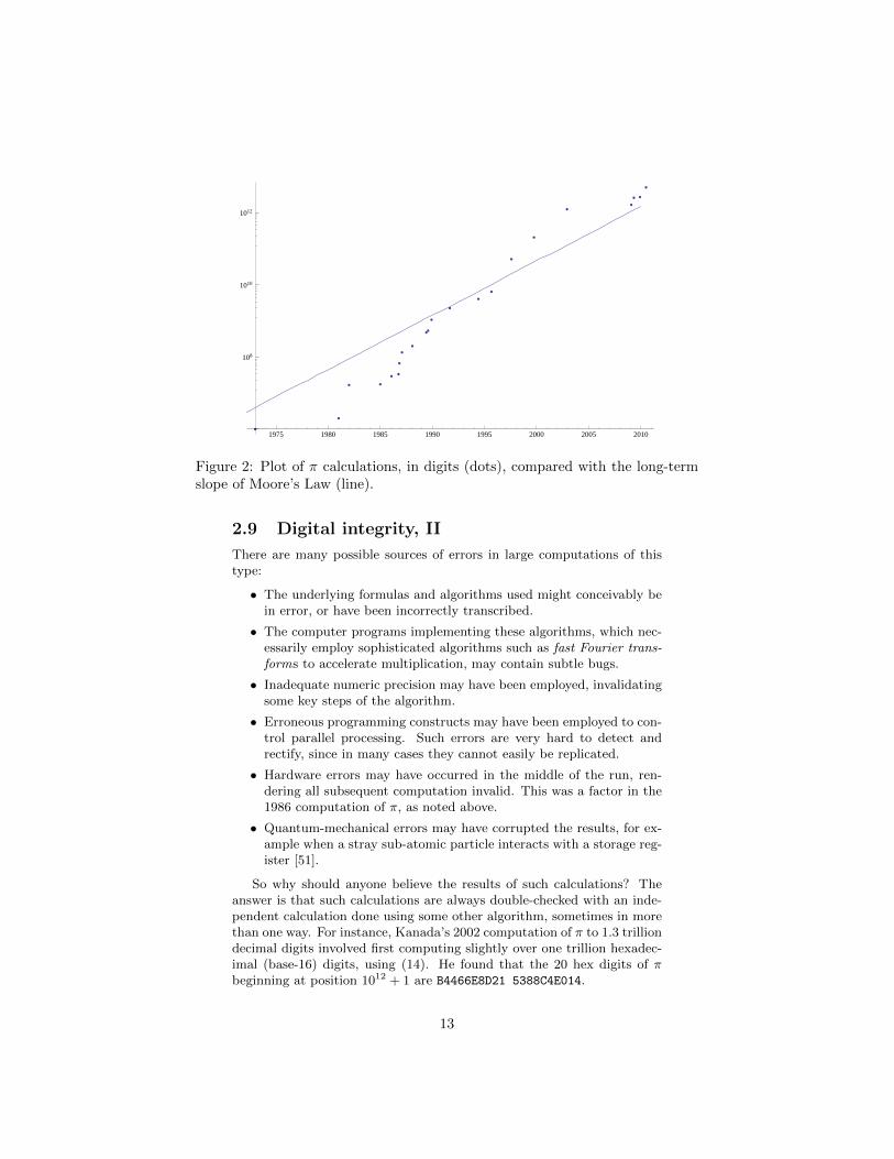
Figure 2 shows the progress of π calculations since 1970, superimposedwith a line that charts the long-term trend of Moore’s Law. It is worthnoting that whereas progress in computing π exceeded Moore’s Law inthe 1990s, it has lagged a bit in the past decade.

5See “12.1 Trillion Digits of Pi And we’re out of disk space...” at http://www.numberworld.org/misc_runs/pi-12t/.

12

1975 1980 1985 1990 1995 2000 2005 2010

108

1010

1012

Figure 2: Plot of π calculations, in digits (dots), compared with the long-termslope of Moore’s Law (line).

2.9 Digital integrity, II

There are many possible sources of errors in large computations of thistype:

• The underlying formulas and algorithms used might conceivably bein error, or have been incorrectly transcribed.

• The computer programs implementing these algorithms, which nec-essarily employ sophisticated algorithms such as fast Fourier trans-forms to accelerate multiplication, may contain subtle bugs.

• Inadequate numeric precision may have been employed, invalidatingsome key steps of the algorithm.

• Erroneous programming constructs may have been employed to con-trol parallel processing. Such errors are very hard to detect andrectify, since in many cases they cannot easily be replicated.

• Hardware errors may have occurred in the middle of the run, ren-dering all subsequent computation invalid. This was a factor in the1986 computation of π, as noted above.

• Quantum-mechanical errors may have corrupted the results, for ex-ample when a stray sub-atomic particle interacts with a storage reg-ister [51].

So why should anyone believe the results of such calculations? Theanswer is that such calculations are always double-checked with an inde-pendent calculation done using some other algorithm, sometimes in morethan one way. For instance, Kanada’s 2002 computation of π to 1.3 trilliondecimal digits involved first computing slightly over one trillion hexadec-imal (base-16) digits, using (14). He found that the 20 hex digits of πbeginning at position 1012 + 1 are B4466E8D21 5388C4E014.

13

Kanada then calculated these same 20 hex digits directly, using the“BBP” algorithm [18]. The BBP algorithm for π is based on the formula

π =

∞∑i=0

1

16i

(4

8i+ 1− 2

8i+ 4− 1

8i+ 5− 1

8i+ 6

), (15)

which was discovered via the PSLQ integer relation algorithm [24, 232–234]. In particular, PSLQ discovered the formula

π = 4 2F1

(1, 1

454

∣∣∣∣− 1

4

)+ 2 tan−1

(1

2

)− log 5, (16)

where 2F1

(1, 1

454

∣∣∣∣− 14

)= 0.955933837 . . . is a Gaussian hypergeometric

function. From (16), the series (15) almost immediately follows. TheBBP algorithm, which is based on (15), permits one to calculate binary orhexadecimal digits of π beginning at an arbitrary starting point, withoutneeding to calculate any of the preceding digits, by means of a simplescheme that requires only modest-precision arithmetic.

The result of the BBP calculation was B4466E8D21 5388C4E014. Need-less to say, in spite of the many potential sources of error in both computa-tions, the final results dramatically agree, thus confirming in a convincingalbeit heuristic sense that both results are almost certainly correct. Al-though one cannot rigorously assign a “probability” to this event, notethat the probability that two 20-long random hex digit strings perfectlyagree is one in 1620 ≈ 1.2089× 1024.

This raises the following question: Which is more securely established,the assertion that the hex digits of π in positions 1012+1 through 1012+20are B4466E8D21 5388C4E014, or the final result of some very difficult workof mathematics that required hundreds or thousands of pages, that reliedon many results quoted from other sources, and that (as is frequently thecase) has been read in detail by only only a relative handful of math-ematicians besides the author? (See also [24, §8.4]). In our opinion,computation often trumps cerebration.

In a 2010 computation using the BBP formula, Tse-Wo Zse of Yahoo!Cloud Computing calculated 256 binary digits of π starting at the twoquadrillionth bit. He then checked his result using the following variantof the BBP formula due to Bellard:

π =1

64

∞∑k=0

(−1)k

1024k

(256

10k + 1+

1

10k + 1− 64

10k + 3− 4

10k + 5

− 4

10k + 7− 32

4k + 1− 1

4k + 3

). (17)

In this case, both computations verified that the 24 hex digits begin-ning immediately after the 500 trillionth hex digit (i.e., after the twoquadrillionth binary bit) are: E6C1294A ED40403F 56D2D764.

In 2012 Ed Karrel using the BBP formula on the CUDA6 system withprocessing to determine that starting after the 1015 position the hex-bits

6See http://en.wikipedia.org/wiki/CUDA.

14

are E353CB3F7F0C9ACCFA9AA215F2. This was done on four NVIDIA GTX690 graphics cards (GPUs) installed in CUDA. Yahoo! ’s run took 23 days;this took 37 days.7

Some related BBP-type computations of digits of π2 and Catalan’sconstant G =

∑n≥1(−1)n/(2n + 1)2 = 0.9159655941 . . . are described

in [17]. In each case, the results were computed two different ways forvalidation. These runs used 737 hours on a 16384-CPU IBM Blue Genecomputer, or, in other words, a total of 1378 CPU-years.

2.10 Formal verification of proof

In 1611, Kepler described the stacking of equal-sized spheres into the fa-miliar arrangement we see for oranges in the grocery store. He assertedthat this packing is the tightest possible. This assertion is now knownas the Kepler conjecture, and has persisted for centuries without rigorousproof. Hilbert implicitly included the irregular case of the Kepler con-jecture in problem 18 of his famous list of unsolved problems in 1900:whether there exist non-regular space-filling polyhedra? the regular casehaving been disposed of by Gauss in 1831.

In 1994, Thomas Hales, now at the University of Pittsburgh, proposeda five-step program that would result in a proof: (a) treat maps that onlyhave triangular faces; (b) show that the face-centered cubic and hexagonal-close packings are local maxima in the strong sense that they have a higherscore than any Delaunay star with the same graph; (c) treat maps thatcontain only triangular and quadrilateral faces (except the pentagonalprism); (d) treat maps that contain something other than a triangular orquadrilateral face; and (e) treat pentagonal prisms.

In 1998, Hales announced that the program was now complete, withSamuel Ferguson (son of mathematician-sculptor Helaman Ferguson) com-pleting the crucial fifth step. This project involved extensive computation,using an interval arithmetic package, a graph generator, and Mathematica.The computer files containing the source code and computational resultsoccupy more than three Gbytes of disk space. Additional details, includingpapers, are available at http://www.math.pitt.edu/~thales/kepler98.For a mixture of reasons—some more defensible than others—the Annalsof Mathematics initially decided to publish Hales’ paper with a cautionarynote, but this disclaimer was deleted before final publication.

Hales [36] has now embarked on a multi-year program to certify theproof by means of computer-based formal methods, a project he hasnamed the “Flyspeck” project.8 As these techniques become better under-stood, we can envision a large number of mathematical results eventuallybeing confirmed by computer, as instanced by other articles in the sameissue of the Annals as Hales’ article. But this will take decades.

7See www.karrels.org/pi/.8He reported in December 2012 at an ICERM workshop that this was nearing completion.

15

3 The experimental paradigm in appliedmathematics

The field of applied mathematics is an enormous edifice, and we cannotpossibly hope, in this short essay, to provide a comprehensive survey ofcurrent computational developments. So we shall limit our discussion towhat may be termed “experimental applied mathematics,” namely employmethods akin to those mentioned above in pure mathematics to problemsthat had their origin in an applied setting. In particular, we will touchmainly on examples that employ either high-precision computation orinteger relation detection, as these tools lead to issues similar to thosealready highlighted above.

First we will examine some historical examples of this paradigm inaction.

3.1 Gravitational boosting or “slingshot magic”

One interesting space-age example is the unexpected discovery of grav-itational boosting by Michael Minovitch, who at the time (1961) was astudent working on a summer project at the Jet Propulsion Laboratoryin Pasadena, California. Minovitch found that Hohmann transfer ellipseswere not, as then believed, the minimum-energy way to reach the outerplanets. Instead, he discovered, by a combination of clever analyticalderivations and heavy-duty computational experiments on IBM 7090 com-puters (which were the world’s most powerful systems at the time), thatspacecraft orbits which pass close by other planets could gain a “slingshoteffect” substantial boost in speed, compensated by an extremely smallchange in the orbital velocity of the planet, on their way to a distant loca-tion. Some of his earlier computation was not supported enthusiasticallyby NASA. As Minovitz later wrote,

Prior to the innovation of gravity-propelled trajectories, itwas taken for granted that the rocket engine, operating onthe well-known reaction principle of Newton’s Third Law ofMotion, represented the basic, and for all practical purposes,the only means for propelling an interplanetary space vehiclethrough the Solar System.9

Without such a boost from Jupiter, Saturn, and Uranus, the Voyagermission would have taken more than 30 years to reach Neptune; instead,Voyager reached Neptune in only ten years. Indeed, without gravitationalboosting, we would still be waiting! We would have to wait much longerfor Voyager to leave the solar system as it now apparently is.

9There are differing accounts of how this principle was discovered; we rely on the first-person account at http://www.gravityassist.com/IAF1/IAF1.pdf. Additional informationon “slingshot magic” is given at http://www.gravityassist.com/ and http://www2.jpl.

nasa.gov/basics/grav/primer.php.

16

3.2 Fractals and chaos

One premier example of 20th century applied experimental mathematicsis the development of fractal theory, as exemplified by the works of BenoitMandelbrot. Mandelbrot studied many examples of fractal sets, many ofthem with direct connections to nature. Applications include analyses ofthe shapes of coastlines, mountains, biological structures, blood vessels,galaxies, even music, art and the stock market. For example, Mandelbrotfound that the coast of Australia, the West Coast of Britain and theland frontier of Portugal all satisfy shapes given by a fractal dimension ofapproximately 1.75.

In the 1960s and early 1970s, applied mathematicians began to compu-tationally explore features of chaotic iterations that had previously beenstudied by analytic methods. May, Lorenz, Mandelbrot, Feigenbaum, Ru-elle, York and others led the way in utilizing computers and graphics toexplore this realm, as chronicled for example in Gleick’s book Chaos: Mak-ing a New Science. By now fractals have found nigh countless uses. In ourown research [12] we have been looking at expectations over self-similarfractals, motivated by modelling rodent brain-neuron geometry.

3.3 The uncertainty principle

Here we examine a principle that, while discovered early in the 20th cen-tury by conventional formal reasoning, could have been discovered muchmore easily with computational tools.

Most readers have heard of the uncertainty principle from quantummechanics, which is often expressed as the fact that the position and mo-mentum of a subatomic-scale particle cannot simultaneously be prescribedor measured to arbitrary accuracy. Others may be familiar with the un-certainty principle from signal processing theory, which is often expressedas the fact that a signal cannot simultaneously be “time-limited” and“frequency-limited.” Remarkably, the precise mathematical formulationsof these two principles are identical (although the quantum mechanicsversion presumes the existence of de Broglie waves).

Consider a real, continuously differentiable, L2 function f(t), whichfurther satisfies |t|3/2+εf(t) → 0 as |t| → ∞ for some ε > 0. (Thisassures convergence of the integrals below.) For convenience, we assumef(−t) = f(t), so the Fourier transform f(x) of f(t) is real, although thisis not necessary. Define

E(f) =

∫ ∞−∞

f2(t) dt V (f) =

∫ ∞−∞

t2f2(t) dt

f(x) =

∫ ∞−∞

f(t)e−itx dt Q(f) =V (f)

E(f)· V (f)

E(f). (18)

Then the uncertainty principle is the assertion that Q(f) ≥ 1/4, with

equality if and only if f(t) = ae−(bt)2/2 for real constants a and b. Theproof of this fact is not terribly difficult but is hardly enlightening—see,for example [24, pg. 183–188].

17

f(t) Interval f(x) Q(f)

1− t sgn t [−1, 1] 2(1− cosx)/x2 3/10

1− t2 [−1, 1] 4(sinx− x cosx)/x3 5/14

1/(1 + t2) [−∞,∞] π exp(−x sgnx) 1/2

e−|t| [−∞,∞] 2/(1 + x2) 1/2

1 + cos t [−π, π] 2 sin(πx)/(x− x3) (π2 − 15/2)/9

Table 1: Q values for various functions.

Let us approach this problem as an experimental mathematician might.As mentioned, it is natural when studying Fourier transforms (particu-larly in the context of signal processing) to consider the “dispersion” ofa function and to compare this with the dispersion of its Fourier trans-form. Noting what appears to be an inverse relationship between thesetwo quantities, we are led to consider Q(f) in (18). With the assistanceof Maple or Mathematica, one can explore examples, as shown in Table 1.Note that each of the entries in the last column is in the range (1/4, 1/2).Can one get any lower?

To further study this problem experimentally, note that the Fouriertransform f of f(t) can be closely approximated with a fast Fourier trans-form, after suitable discretization. The integrals V and E can be similarlyevaluated numerically.

Then one can adopt a search strategy to minimize Q(f), starting, say,with a “tent function,” then perturbing it up or down by some ε on aregular grid with spacing δ, thus creating a continuous, piecewise linearfunction. When for a given δ, a minimizing function f(t) has been found,reduce ε and δ, and repeat. Terminate when δ is sufficiently small, say10−6 or so. (For details, see [24].)

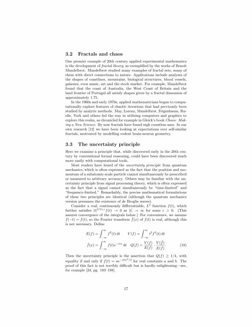
The resulting function f(t) is shown in Figure 3. Needless to say, itsshape strongly suggests a Gaussian probability curve. Figure 3 actually

shows both f(t) and the function e−(bt)2/2, where b = 0.45446177: theyare identical to the resolution of the plot!

In short, it is a relatively simple matter, using 21st-century computa-tional tools, to numerically “discover” the signal-processing form of theuncertainty principle. Doubtless the same is true of many other historicalprinciples of physics, chemistry and other fields, thus illustrating items 1,2, 3 and 4 at the start of Section 2.

3.4 Chimera states in oscillator arrays

It is fair to say that the computational-experimental approach in appliedmathematics has greatly accelerated in the 21st century. We show herea few specific illustrative examples. These include several by the presentauthors, because we are familiar with them. There are doubtless manyothers that we are not aware of that are similarly exemplary of the exper-imental paradigm.

One interesting example was the 2002 discovery by Kuramoto, Bat-togtokh, and Sima of “chimera” states, which arise in arrays of identicaloscillators, where individual oscillators are correlated with oscillators some

18

−8 −6 −4 −2 0 2 4 6 80

0.1

0.2

0.3

0.4

0.5

0.6

0.7

0.8

0.9

1

Figure 3: Q-minimizer and matching Gaussian (identical to the plot resolution).

distance away in the array. These systems can arise in a wide range ofphysical systems, including Josephson junction arrays, oscillating chem-ical systems, epidemiological models, neural networks underlying snailshell patterns, and “ocular dominance stripes” observed in the visual cor-tex of cats and monkeys. In chimera states, named for the mythologicalbeast that incongruously combines features of lions, goats and serpents,the oscillator array bifurcates into two relatively stable groups, the firstcomposed of coherent, phased-locked oscillators, and the second composedof incoherent, drifting oscillators.

According to Abrams and Strogatz, who subsequently studied thesestates in detail, most arrays of oscillators quickly converge into one of fourtypical patterns: (a) synchrony, with all oscillators moving in unison; (b)solitary waves in one dimension or spiral waves in two dimensions, withall oscillators locked in frequency; (c) incoherence, where phases of theoscillators vary quasi-periodically, with no global spatial structure; and (d)more complex patterns, such as spatiotemporal chaos and intermittency.But in chimera states, phase locking and incoherence are simultaneouslypresent in the same system.

The simplest governing equation for a continuous one-dimensionalchimera array is

∂φ

∂t= ω −

∫ 1

0

G(x− x′) sin[φ(x, t)− φ(x′, t) + α

]dx′, (19)

where φ(x, t) specifies the phase of the oscillator given by x ∈ [0, 1) attime t, and G(x − x′) specifies the degree of nonlocal coupling betweenthe oscillators x and x′. A discrete, computable version of (19) can beobtained by replacing the integral with a sum over a 1-D array (xk, 0 ≤k < N), where xk = k/N . Kuramoto and Battogtokh took G(x − x′) =C exp(−κ|x− x′|) for constant C and parameter κ.

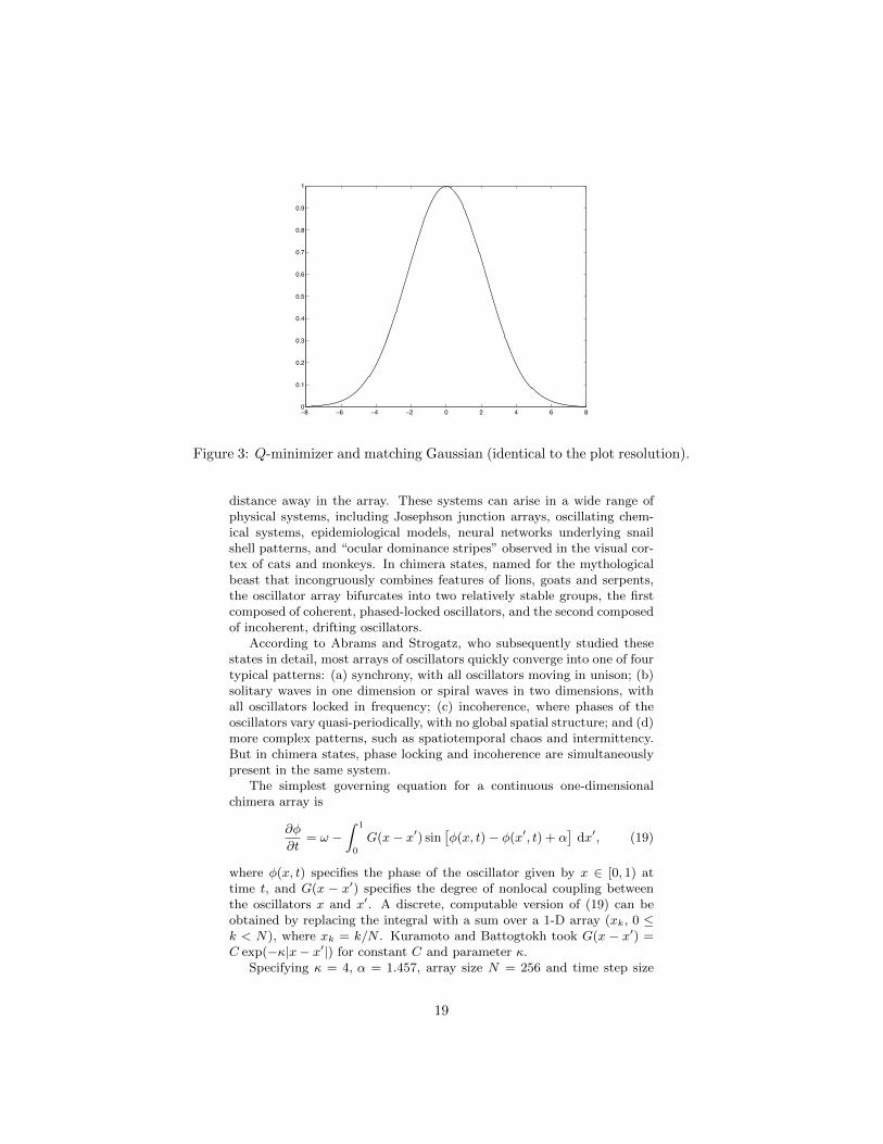
Specifying κ = 4, α = 1.457, array size N = 256 and time step size

19

Figure 4: Phase of oscillations for a chimera system. The x-axis runs from 0 to1 with periodic boundaries.

∆t = 0.025, and starting from φ(x) = 6 exp[−30(x− 1/2)2

]r(x), where

r is a uniform random variable on [−1/2, 1/2), gives rise to the phasepatterns shown in Figure 4. Note that the oscillators near x = 0 andx = 1 appear to be phase-locked, moving in near-perfect synchrony withtheir neighbors, but those oscillators in the center drift wildly in phase,both with respect to their neighbors and to the locked oscillators.

Numerous researchers have studied this phenomenon since its initialnumerical discovery. Abrams and Strogatz studied the coupling functionis given G(x) := (1 + A cosx)/(2π), where 0 ≤ A ≤ 1, for which theywere able to solve the system analytically, and then extended their meth-ods to more general systems. They found that chimera systems have acharacteristic life cycle: a uniform phase-locked state, followed by a spa-tially uniform drift state, then a modulated drift state, then the birth ofa chimera state, followed a period of stable chimera, then a saddle-nodebifurcation, and finally an unstable chimera.10

3.5 Winfree oscillators

One closely related development is the resolution of the Quinn-Rand-Strogatz (QRS) constant. Quinn, Rand and Strogatz had studied theWinfree model of coupled nonlinear oscillators, namely

θi = ωi +κ

N

N∑j=1

−(1 + cos θj) sin θi (20)

for 1 ≤ i ≤ N , where θi(t) is the phase of oscillator i at time t, theparameter κ is the coupling strength, and the frequencies ωi are drawnfrom a symmetric unimodal density g(w). In their analyses, they were led

10Various movies can be found on line. For example, http://dmabrams.esam.

northwestern.edu/pubs/ngeo-video1.mov and http://dmabrams.esam.northwestern.edu/

pubs/ngeo-video2.mov show two for groundwater flow.

20

to the formula

0 =

N∑i=1

(2√

1− s2(1− 2(i− 1)/(N − 1))2

− 1√1− s2(1− 2(i− 1)/(N − 1))2

),

implicitly defining a phase offset angle φ = sin−1 s due to bifurcation. Theauthors conjectured, on the basis of numerical evidence, the asymptoticbehavior of the N -dependent solution s to be

1− sN ∼c1N

+c2N2

+c3N3

+ · · · ,

where c1 = 0.60544365 . . . is now known as the QRS constant.In 2008, the present authors together with Richard Crandall computed

the numerical value of this constant to 42 decimal digits, obtaining

c1 ≈ 0.60544365719673274947892284244 . . . .

With this numerical value in hand, they were able to demonstrate that c1is the unique zero of the Hurwitz zeta function ζ(1/2, z/2) on the interval0 ≤ z ≤ 2. What’s more, they found that c2 = −0.104685459 . . . is givenanalytically by

c2 = c1 − c21 − 30ζ(−1/2, c1/2)

ζ(3/2, c1/2).

In this case experimental computation led to a closed form which couldthen be used to establish the existence and form of the critical point, thusengaging at the very least each of items #1 through #6 of our ‘mathodol-ogy’, and highlighting the interplay between computational discovery andtheoretical understanding.

3.6 High precision dynamics

Periodic orbits form the “skeleton” of a dynamical system and providemuch useful information, but when the orbits are unstable, high-precisionnumerical integrators are often required to obtain numerically meaningfulresults.

For instance, Figure 5 shows computed symmetric periodic orbits forthe (7 + 2)-Ring problem using double and quadruple precision. The(n + 2)-body Ring problem describes the motion of an infinitesimal par-ticle attracted by the gravitational field of n + 1 primary bodies, n ofthem at the vertices of a regular n-gon rotating in its own plane aboutthe central body with constant angular velocity. Each point correspondsto the initial conditions of one symmetric periodic orbit, and the greyarea corresponds to regions of forbidden motion (delimited by the limitcurve). To avoid “false” initial conditions it is useful to check if the initialconditions generate a periodic orbit up to a given tolerance level; but forhighly unstable periodic orbits double precision is not enough, resulting in

21

−5 −4 −3 −2 −1 0 1 2−8

−7

−6

−5

−4

coordinate x

Jaco

bi c

onst

ant C

−5 −4 −3 −2 −1 0 1 2−8

−7

−6

−5

−4

coordinate x

Jaco

bi c

onst

ant C

limitm=1m=2m=3m=4

B

A

Figure 5: Symmetric periodic orbits (m denotes multiplicity of the periodic orbit) in

the most chaotic zone of the (7 + 2)-Ring problem using double (A) and quadruple

(B) precision. Note “gaps” in the double precision plot. (Reproduced by permission.)

gaps in the figure that are not present in the more accurate quad precisionrun.

Hundred-digit precision arithmetic plays a fundamental role in a 2010study of the fractal properties of the Lorenz attractor [3.xy] (seeFigure 6). The first plot shows the intersection of an arbitrary trajectoryon the Lorenz attractor with the section z = 27, in a rectangle in the x−yplane. All later plots zoom in on a tiny region (too small to be seen bythe unaided eye) at the center of the red rectangle of the preceding plotto show that what appears to be a line is in fact many lines.

Figure 6: Fractal property of the Lorenz attractor. (Reproduced by permission.)

The Lindstedt-Poincare method for computing periodic orbits is basedon the Lindstedt-Poincare perturbation theory, Newton’s method for solv-ing nonlinear systems, and Fourier interpolation. Viswanath has used this

22

in combination with high-precision libraries to obtain periodic orbits forthe Lorenz model at the classical Saltzman’s parameter values. This pro-cedure permits one to compute, to high accuracy, highly unstable periodicorbits more efficiently than with conventional schemes, in spite of the addi-tional cost of high-precision arithmetic. For these reasons, high-precisionarithmetic plays a fundamental role in the study of the fractal propertiesof the Lorenz attractor (see Figures 6 and 7), and in the consistent formaldevelopment of complex singularities of the Lorenz system using infiniteseries. For additional details and references, see [5].

0 200 400 600 800 100010

−2

100

102

104

−log10

|error|

CPU

tim

e

Lorenz model

1 2 3 4 5 6 7 8 9100

101

102

103

number of iterations

−lo

g 10|E

rror

|Lorenz model

Quadratic convergence

LRLLRLR

LRLLRLR

O(log (precision)4 )10

Figure 7: Computational relative error vs. CPU time and number of iterations in a

1000-digit computation of the periodic orbits LR and LLRLR of the Lorenz model.

(Reproduced by permission.)

3.7 Snow crystals

Computational experimentation has even been useful in the study ofsnowflakes. In a 2007 study, Janko Gravner and David Griffeath used asophisticated computer-based simulator to study the process of formationof these structures, known in the literature as snow crystals and infor-mally as snofakes. Their model simulated each of the key steps, includingdiffusion, freezing, and attachment, and thus enabled researchers to study,dependence on melting parameters. Snow crystals produced by their sim-ulator vary from simple stars, to six-sided crystals with plate-ends, tocrystals with dendritic ends, and look remarkably similar to natural snowcrystals. Among the findings uncovered by their simulator is the fact thatthese crystals exhibit remarkable overall symmetry, even in the process ofdynamically changing parameters. Their simulator is publicly availableat http://psoup.math.wisc.edu/Snofakes.htm.

The latest developments in computer and video technologyhave provided a multiplicity of computational and symbolictools that have rejuvenated mathematics and mathematics ed-ucation. Two important examples of this revitalization areexperimental mathematics and visual theorems. [38]

3.8 Visual mathematics

J. E. Littlewood (1885-1977) wrote [41]

23

Figure 8: Seeing often can and should be believing.

A heavy warning used to be given [by lecturers] that picturesare not rigorous; this has never had its bluff called and has per-manently frightened its victims into playing for safety. Somepictures, of course, are not rigorous, but I should say most are(and I use them whenever possible myself).

This was written in 1953, long before the current graphics, visualizationand dynamic geometric tools (such as Cinderella or Geometer’s Sketch-pad) were available.

The ability to “see” mathematics and mathematical algorithms as im-ages, movies or simulations is more-and-more widely used (as indeed wehave illustrated in passing), but is still under appreciated. This is truefor algorithm design and improvement and even more fundamentally asa tool to improve intuition, and as a resource when preparing or givinglectures.

3.9 Iterative methods for protein confirmation

In [2] we applied continuous convex optimization tools (alternating pro-jection and alternating reflection algorithms) to a large class of nonconvexand often highly combinatorial image or signal reconstruction problems.The underlying idea is to consider a feasibility problem that asks for apoint in the intersection C := C1 ∩C2 of two sets C1 and C2 in a Hilbertspace.

The method of alternating projections (MAP) is to iterate

xn 7→ yn = PC1(xn) 7→ PC2(yn) =: xn+1.

24

Here PA(x) := {y ∈ A : ‖x − y‖ = infa∈A ‖x − a‖ := dA(x)} is thenearest point (metric) projection. The reflection is given by RA(x) :=

2x − PA(x), (PA(x) = x+RA(x)2

), and the most studied Douglas-Rachfordreflection method (DR) can be described by

xn 7→ yn = RC1(xn) 7→ zn = RC2(yn) 7→ zn + xn2

=: xn+1

This is nicely captured as ‘reflect-reflect-average.’In practice, for any such method, one set will be convex and the other

sequesters non-convex information.11 It is most useful when projectionson the two sets are relatively easy to estimate but the projection on theintersection C is inaccessible. The methods often work unreasonably wellbut there is very little theory unless both sets are convex. For example, theoptical aberration problem in the original Hubble telescope was ‘fixed’ byan alternating projection phase retrieval method (by Fienup and others),before astronauts could actually physically replace the mis-ground lens.

3.9.1 Protein confirmation

We illustrate the situation with reconstruction of protein structure usingonly the short distances below about six Angstroms12 between atoms thatcan be measured by nondestructive MRI techniques. This can viewed as aEuclidean distance matrix completion problem [2], so that only geometry(and no chemistry) is directly involved. That is, we ask the algorithm topredict a configuration in 3-space that is consistent with the given shortdistances.

Average (maximum) errors from five replications with re-flection methods of six proteins taken from a standard database.

Protein # Atoms Rel. Error (dB) RMSE Max Error

1PTQ 404 -83.6 (-83.7) 0.0200 (0.0219) 0.0802 (0.0923)1HOE 581 -72.7 (-69.3) 0.191 (0.257) 2.88 (5.49)1LFB 641 -47.6 (-45.3) 3.24 (3.53) 21.7 (24.0)1PHT 988 -60.5 (-58.1) 1.03 (1.18) 12.7 (13.8)1POA 1067 -49.3 (-48.1) 34.1 (34.3) 81.9 (87.6)1AX8 1074 -46.7 (-43.5) 9.69 (10.36) 58.6 (62.6)

What do the reconstructions look like? We turn to graphicinformation for 1PTQ and 1POA which were respectively our most andleast successful cases.

11When the set A is non-convex the projection PA(x) may be a set and we must insteadselect some y ∈ PA(x).

12Interatomic distances below 6A typically constitute less than 8% of the total distancesbetween atoms in a protein.

25

1PTQ (actual) 5,000 steps, -83.6dB (perfect)

1POA (actual) 5,000 steps, -49.3dB (mainly good!)

Note that the failure (and large mean or max error) is caused by avery few very large spurious distances. The remainder is near perfect.Below we show the radical visual difference in the behavior of reflectionand projection methods on IPTQ.

While traditional numerical measures (relative error in decibels, rootmean square error, and maximum error) of success held some informa-tion, graphics-based tools have been dramatically more helpful. It is visu-ally obvious that this method has successfully reconstructed the proteinwhereas the MAP reconstruction method, shown below, has not. This dif-ference is not evident if one compares the two methods in terms of decibelmeasurement (beloved of engineers).

Douglas–Rachford reflection (DR) reconstruction: (of IPTQ13)

500 steps, -25 dB. 1,000 steps, -30 dB. 2,000 steps, -51 dB. 5,000 steps, -84 dB.

After 1000 steps or so, the protein shape is becoming apparent. After 2000steps only minor detail is being fixed. Decibel measurement really doesnot discriminate this from the failure of the MAP method below whichafter 5000 steps has made less progress than DR after 1000.

Alternating projection (MAP) reconstruction: (of IPTQ)

13The first 3,000 steps of the 1PTQ reconstruction are available as a movie at http://

carma.newcastle.edu.au/DRmethods/1PTQ.html.

26

500 steps, -22 dB. 1,000 steps, -24 dB. 2,000 steps, -25 dB. 5,000 steps, -28 dB.

Yet MAP works very well for optical abberation correction of the Hub-ble telescope and the method is now built in to amateur telescope soft-ware. This problem-specific variation in behavior is well observed butpoorly understood; it is the heart of our current studies.

3.10 Mathematical finance

Coincident with the rise of powerful computational hardware, sophisti-cated mathematical techniques are now being employed to analyze mar-ket data in real-time and generate profitable investment strategies. Thisapproach, commonly known as “quantitative” or “mathematical” finance,often involves computationally exploring a wide range of portfolio optionsor investment strategies [40, 30].

One interesting aspect of these studies is the increasing realization ofhow easy it is to “over-compute” an investment strategy, in a statisticalsense. For example, one common approach to finding an effective quan-titative investment strategy is to tune the strategy on historical data (a“backtest”). Unfortunately, financial mathematicians are finding that be-yond a certain point, examining thousands or millions of variations of aninvestment strategy (which is certainly possible with today’s computertechnology) to find the optimal strategy may backfire, because the result-ing scheme may “overfit” the backtest data—the optimal strategy willwork well only with a particular set of securities or over a particular timeframe (in the past!). Indeed, backtest overfitting is now thought to be oneof the primary reasons that an investment strategy which looks promisingon paper often falls flat in real-world practice [15, 16].

3.11 Digital integrity III

Difficulties with statistical overfitting in financial mathematics can beseen as just one instance of the larger challenge of ensuring that results ofcomputational experiments are truly valid and reproducible, which, afterall, is the bedrock of all scientific research. We discussed these issues inthe context of pure mathematics in Section 2.9, but there are numerousanalogous concerns in applied mathematics:

• Whether the calculation is numerically reproducible, i.e., whetheror not the computation produces results acceptably close to thoseof an equivalent calculation performed using different hardware orsoftware. In some cases, more stable numerical algorithms or higher-precision arithmetic may be required for certain portions of the com-putation to ameliorate such difficulties.

• Whether the calculation has been adequately validated with inde-pendently written programs or distinct software tools.

27

• Whether the calculation has been adequately validated by compari-son with empirical data (where possible).

• Whether the algorithms and computational techniques used in thecalculation have been documented sufficiently well in journal articlesor publicly accessible repositories, so that an independent researchercan reproduce the stated results.

• Whether the code and/or software tool itself has been secured in apermanent repository.

These issues were addressed in a 2012 workshop held at the Institutefor Computational and Experimental Research in Mathematics (ICERM).See [51] for details.

4 Additional examples of the experimen-tal paradigm in action

4.1 Giuga’s conjecture

As another measure of what changes over time and what doesn’t, considerGiuga’s conjecture:

Giuga’s conjecture (1950): An integer n > 1, is a prime if and onlyif Gn :=

∑n−1k=1 k

n−1 ≡ n− 1 mod n.This conjecture is not yet proven. But it is known that any counterex-

amples are necessarily Carmichael numbers—square free ‘pseudo-primenumbers’—and much more. These rare birds were only proven infinite innumber in 1994. In [25, pp. 227], we exploited the fact that if a numbern = p1 · · · pm with m > 1 prime factors pi is a counterexample to Giuga’sconjecture (that is, satisfies Gn ≡ n − 1 mod n), then for i 6= j we havethat pi 6= pj , that

m∑i=1

1

pi> 1,

and that the pi form a normal sequence: pi 6≡ 1 mod pj for i 6= j.Thus, the presence of ‘3’ excludes 7, 13, 19, 31, 37, . . . , and of ‘5’ excludes11, 31, 41, . . ..

This theorem yielded enough structure, using some predictive exper-imentally discovered heuristics, to build an efficient algorithm to show—over several months in 1995—that any counterexample had at least 3459prime factors and so exceeded 1013886, extended a few years later to 1014164

in a five-day desktop computation. The heuristic is self-validating everytime that the programme runs successfully. But this method necessarilyfails after 8135 primes; at that time we hoped to someday exhaust its use.

In 2010, one of us was able to obtain almost as good a bound of 3050primes in under 110 minutes on a laptop computer, and a bound of 3486primes and 14,000 digits in less than 14 hours; this was extended to 3,678primes and 17,168 digits in 93 CPU-hours on a Macintosh Pro, usingMaple rather than C++, which is often orders-of-magnitude faster butrequires much more arduous coding. In 2013, the same one of us with his

28

students revisited the computation and the time and space requirementsfor further progress [27]. Advances in multi-threading tools and goodPython tool kits, along with Moore’s law, made the programming mucheasier and allowed the bound to be increased to 19,908 digits. This studyalso indicated that we are unlikely to exhaust the method in our lifetime.

4.2 Lehmer’s conjecture

An equally hard number-theory related conjecture, for which much lessprogress can be recorded, is the following. Here φ(n) is Euler’s totientfunction, namely the number of positive integers less than or equal to nthat are relatively prime to n:

Lehmer’s conjecture (1932). φ(n)∣∣(n − 1) if and only if n is prime.

Lehmer called this “as hard as the existence of odd perfect numbers.”Again, no proof is known of this conjecture, but it has been known

for some time that the prime factors of any counterexample must forma normal sequence. Now there is little extra structure. In a 1997 SimonFraser M.Sc. thesis, Erick Wong verified the conjecture for 14 primes,using normality and a mix of PARI, C++ and Maple to press the boundsof the “curse of exponentiality.” This very clever computation subsumedthe entire scattered literature in one computation, but could only extendthe prior bound from 13 primes to 14.

For Lehmer’s related 1932 question: when does φ(n) | (n+ 1)?, Wongshowed there are eight solutions with no more than seven factors (six-factor solutions are due to Lehmer). Let

Lm :=

m−1∏k=0

Fk

with Fn := 22n + 1 denoting the Fermat primes. The solutions are

2,L1,L2, . . . ,L5,

and the rogue pair 4919055 and 6992962672132095, but analyzing justeight factors seems out of sight. Thus, in 70 years the computer onlyallowed the exclusion bound to grow by one prime.

In 1932 Lehmer couldn’t factor 6992962672132097. If it had beenprime, a ninth solution would exist: since φ(n)|(n + 1) with n + 2 primeimplies that N := n(n+2) satisfies φ(N)|(N+1). We say couldn’t becausethe number is divisible by 73; which Lehmer—a father of much factoriza-tion literature–could certainly have discovered had he anticipated a smallfactor. Today, discovering that

6992962672132097 = 73 · 95794009207289

is nearly instantaneous, while fully resolving Lehmer’s original questionremains as hard as ever.

29

4.3 Inverse computation and Apery-like series

Three intriguing formulae for the Riemann zeta function are

(a) ζ(2) = 3

∞∑k=1

1

k2(2kk

) , (b) ζ(3) =5

2

∞∑k=1

(−1)k+1

k3(2kk

) , (21)

(c) ζ(4) =36

17

∞∑k=1

1

k4(2kk

) .Binomial identity (21)(a) has been known for two centuries, while (b)—exploited by Apery in his 1978 proof of the irrationality of ζ(3)—wasdiscovered as early as 1890 by Markov, and (c) was noted by Comtet [11].

Using integer relation algorithms, bootstrapping, and the “Pade” func-tion (Mathematica and Maple both produce rational approximations well),in 1996 David Bradley and one of us [11, 25] found the following unantic-ipated generating function for ζ(4n+ 3):

∞∑k=0

ζ(4k + 3)x4k =5

2

∞∑k=1

(−1)k+1

k3(2kk

)(1− x4/k4)

k−1∏m=1

(1 + 4x4/m4

1− x4/m4

). (22)

Note that this formula permits one to read off an infinity of formulasfor ζ(4n + 3), for n = 0, 1, 2, . . . beginning with (21)(b), by comparingcoefficients of x4k on both sides of the identity.

A decade later, following a quite analogous but much more deliberateexperimental procedure, as detailed in [11], we were able to discover asimilar general formula for ζ(2n+ 2) that is pleasingly parallel to (22):

∞∑k=0

ζ(2k + 2)x2k = 3

∞∑k=1

1

k2(2kk

)(1− x2/k2)

k−1∏m=1

(1− 4x2/m2

1− x2/m2

). (23)

As with (22), one can now read off an infinity of formulas, beginning with(21)(a). In 1996, the authors could reduce (22) to a finite form (24) thatthey could not prove,

n∑k=1

2n2

k2

n−1∏i=1

(4k4 + i4)∏ni=1i6=k

(k4 − i4)=

(2n

n

), (24)

but Almqvist and Granville did find a proof a year later. Both Maple andMathematica can now prove identities like (24). Indeed, one of the valuesof such research is that it pushes the boundaries of what a CAS can do.

Shortly before his death, Paul Erdos was shown the form (24) at ameeting in Kalamazoo. He was ill and lethargic, but he immediatelyperked up, rushed off, and returned 20 minutes later saying excitedly thathe had no idea how to prove (24), but that if proven it would have impli-cations for the irrationality of ζ(3) and ζ(7). Somehow in 20 minutes anunwell Erdos had intuited backwards our whole discovery process. Sadly,no one has yet seen any way to learn about the irrationality of ζ(4n+ 3)from the identity, and Erdos’s thought processes are presumably as dissim-ilar from computer-based inference engines as Kasparov’s are from thoseof the best chess programs.

30

A decade later, the Wilf-Zeilberger algorithm [53, 46]—for which theinventors were awarded the Steele Prize—directly (as implemented inMaple) certified (23) [24, 25]. In other words, (23) was both discoveredand proven by computer. This is the experimental mathematician’s “holygrail” (item 6 in the list at the beginning of Section 2), though it wouldhave been even nicer to be led subsequently to an elegant human proof.That preference may change as future generations begin to take it forgranted that the computer is a collaborator.

We found a comparable generating function for ζ(2n+ 4), giving (21)(c) when x = 0, but one for ζ(4n+ 1) still eludes us.

4.4 Ising integrals

High-precision has proven essential in studies with Richard Crandall (see[24, 9]) of the following integrals:

Cn =4

n!

∫ ∞0

· · ·∫ ∞0

1(∑nj=1(uj + 1/uj)

)2 dU,

Dn =4

n!

∫ ∞0

· · ·∫ ∞0

∏i<j

(ui−uj

ui+uj

)2(∑n

j=1(uj + 1/uj))2 dU,

En = 2

∫ 1

0

· · ·∫ 1

0

∏1≤j<k≤n

uk − ujuk + uj

2

dT,

where dU = du1u1· · · dun

un, dT = dt2 · · ·dtn, and uk =

∏ki=1 ti. Note that

En ≤ Dn ≤ Cn.The Dn arise in the Ising theory of mathematical physics and the

Cn in quantum field theory. As far as we know the En are an entirelymathematical construct introduced to study Dn. Direct computation ofthese integrals from their defining formulas is very difficult, but for Cn itcan be shown that

Cn =2n

n!

∫ ∞0

pKn0 (p) dp,

where K0 is the modified Bessel function. Indeed, it is in this form thatCn arises in quantum field theory, as we subsequently learned from DavidBroadhurst. We had introduced it to studyDn. Again an uncanny parallelarises between mathematical inventions and physical discoveries.

Then 1000-digit numerical values so computed were used with PSLQto deduce results such as C4 = 7ζ(3)/12, and furthermore to discover that

limn→∞

Cn = 0.63047350 . . . = 2e−2γ ,

with additional higher-order terms in an asymptotic expansion. One in-

31

triguing experimental result (not then proven) is the following:

E5?= 42− 1984 Li4

(1

2

)+

189π4

10− 74ζ(3)

− 1272ζ(3) log 2 + 40π2 log2 2− 62π2

3

+40π2 log 2

3+ 88 log4 2 + 464 log2 2− 40 log 2, (25)

found by a multi-hour computation on a highly parallel computer system,and confirmed to 250-digit precision. Here Li4(z) =

∑k≥1 z

k/k4 is thestandard order-4 polylogarithm. We also provided 250 digits of E6.

In 2013 Erik Panzer was able to formally evaluate all the En in termsof the alternating multi zeta values [45]. In particular, the experimentalresult for E5 was confirmed, and our high precision computation of E6

was used to confirm Panzer’s evaluation

E6 = 86− 88 log 2 + 768 log4 2 +704

3log3 2 + 1360 log2 2− 13964 ζ2ζ3

− 348 ζ2 − 6048 ζ1,−3 + 134 ζ3 +53775

2ζ5 + 27904 ζ1,1,−3 + 830 ζ2

2

− 2632 log 2 ζ3 − 272 log 2ζ2 + 512 log2 2 ζ2 +1024

3log3 2 ζ2 + 384 log2 2 ζ3

− 3216

5log 2 ζ22 + 11520 log 2ζ1,−3 −

4096

15log5 2, (26)

where ζ3 is a short hand for ζ(3) etc.Here again we see true experimental applied mathematics, wherein our

conjecture (25) and our numerical data for (26) (think of this as preparedbiological sample) was used to confirm further discovery and proof byanother researcher. Equation (26) was automatically converted to Latexfrom Panzer’s Maple worksheet.

Maple does a lovely job of producing correct but inelegant TEX. Inour experience many (largely predictable) errors creep in while trying toprettify such output. For example, as in (1), while 704/3 might have been70/43, it is less likely that a basis element is entirely garbled (althougha power might be wrong). Errors are more likely to occur in trying todirectly handle the TEX for complex expressions produced by computeralgebra systems.

4.5 Ramble integrals and short walks

Consider, for complex s, the n-dimensional ramble integrals [10]

Wn(s) =

∫[0,1]n

∣∣∣∣∣n∑k=1

e2πxki

∣∣∣∣∣s

dx, (27)

which occur in the theory of uniform random walk integrals in the plane,where at each step a unit-step is taken in a random direction as firststudied by Pearson (who did discuss ‘rambles’), Rayleigh and others ahundred years ago. Integrals such as (27) are the s-th moment of thedistance to the origin after n steps. As is well known, various types of

32

random walks arise in fields as diverse as aviation, ecology, economics,psychology, computer science, physics, chemistry, and biology.

In 2010–2012 work (by J. Borwein, A. Straub , J. Wan and W. Zudilin),using a combination of analysis, probability, number theory and high-precision numerical computation, produced results such as

W ′n(0) = −n∫ ∞0

log(x)Jn−10 (x)J1(x)dx,

were obtained, where Jn(x) denotes the Bessel function of the first kind.These results, in turn, lead to various closed forms and have been used toconfirm, to 600-digit precision, the following Mahler measure conjectureadapted from Villegas:

W′5(0)

?=

(15

4π2

)5/2 ∫ ∞0

{η3(e−3t)η3(e−5t)

+η3(e−t)η3(e−15t)}t3 dt,

where the Dedekind eta-function can be computed from: η(q) =

q1/24∏n≥1

(1− qn) = q1/24∞∑

n=−∞

(−1)nqn(3n+1)/2.

There are remarkable and poorly understood connections between di-verse parts of pure, applied and computational mathematics lying be-hind these results. As often there is a fine interplay between devel-oping better computational tools—especially for special functions andpolylogarithms—and discovering new structure.

4.6 Densities of short walks

One of the deepest 2012 discoveries is the following closed form for theradial density p4(α) of a four step uniform random walk in the plane: For2 ≤ α ≤ 4 one has the real hypergeometric form:

p4(α) =2

π2

√16− α2

α3F2

(12, 12, 12

56, 76

∣∣∣∣(16− α2

)3108α4

).

Remarkably, p4(α) is equal to the real part of the right side of this iden-tity everywhere on [0, 4] (not just on [2, 4]), as plotted in Figure 9. Thiswas an entirely experimental discovery—involving at least one fortunateerror—but is now fully proven.

4.7 Moments of elliptic integrals

The previous study on ramble integrals also led to a comprehensive anal-ysis of moments of elliptic integral functions of the form:∫ 1

0

xn0Kn1(x)K′n2(x)En3(x)E′n4(x)dx,

33

Figure 9: The “shark-fin” density of a four step walk.

where the elliptic functions K,E and their complementary versions are

K(x) =

∫ 1

0

dt√(1− t2)(1− x2t2)

,

E(x) =

∫ 1

0

√1− x2t2√1− t2

dt,

K′(x) = K(√

1− x2), E′(x) = E(√

1− x2).

Computations of these integrals to 3200-digit precision, combined withsearches for relations using the PSLQ algorithm, yielded thousands ofunexpected relations among these integrals (see [10]). The scale of thecomputation was required by the number of integrals under simultaneousinvestigation.

4.8 Computation and Constructivism

The fact that (√2√2)√2

=√

22

= 2

provides a one line proof that there exist irrational numbers α and β

such that αβ is rational. Indeed, either (a)√

2√2

is rational or (b) it isirrational; and can play the role of α. This lovely example of the principleof the excluded middle is rejected by constructivists and intuitionists alike.Indeed (b) holds but a constructive proof of such fact is quite elaborate.This is discussed in more detail in [24, §2.9] and [22].

Here we want to make the point that a computational sensibility leadsone to want to know which case occurs, both for existential reasons, andbecause any algorithm with a conditional (if–then) step is probably worth-less if one cannot determine which step to take.

4.9 Limits of computation

As we noted above, experimental studies have raised the question ofwhether one can truly trust—in the mathematical sense—the result of

34

a computation, since there are many possible sources of errors: unreliablenumerical algorithms; bug-ridden computer programs implementing thesealgorithms; system software or compiler errors; hardware errors, either inprocessing or storage; insufficient numerical precision; and obscure errorsof hardware, software or programming that surface only in particularlylarge or difficult computations. Thus when applying experimental meth-ods, it is essential to utilize rigorous validity checks, such as computing akey result by two completely different algorithms, and verifying that theyproduce the same result.

Along this line, it is important to keep in mind that even high-precisionnumerical evaluations can sometimes mislead. One remarkable exampleis the following:∫ ∞

0

cos(2x)

∞∏n=1

cos(x/n) dx = (28)

0.392699081698724154807830422909937860524645434187231595926 . . .

The computation of this integral to high precision can be performed us-ing a scheme described in [14]. When we first did this computation, wethought that the result was π/8, but upon careful checking with the nu-merical value

0.392699081698724154807830422909937860524646174921888227621 . . . ,

it is clear that the two values disagree beginning with the 43rd digit!The late Richard Crandall [29, §7.3] later explained this mystery. By

employing a physically motivated analysis of running out of fuel randomwalks, he showed that π/8 is given by the following very rapidly convergentseries expansion, of which formula (28) above is merely the first term:

π

8=

∞∑m=0

∫ ∞0

cos[2(2m+ 1)x]

∞∏n=1

cos(x/n) dx. (29)

Two terms of the series above suffice for 500-digit agreement.As a final sobering example in this section, we offer the following

“sophomore’s dream” identity

σ29 :=

∞∑n=−∞

sinc(n) sinc(n/3) sinc(n/5) · · · sinc(n/23) sinc(n/29)

=

∫ ∞−∞

sinc(x) sinc(x/3) sinc(x/5) · · · sinc(x/23) sinc(x/29) dx,

(30)

where the denominators range over the odd primes, which was first dis-covered empirically. More generally, consider

σp :=

∞∑n=−∞

sinc(n) sinc(n/3) sinc(n/5) sinc(n/7) · · · sinc(n/p)

?=

∫ ∞−∞

sinc(x) sinc(x/3) sinc(x/5) sinc(x/7) · · · sinc(x/p) dx.

(31)

35

Provably, the following is true: The “sum equals integral” identity,for σp remains valid at least for p among the first 10176 primes; but stopsholding after some larger prime, and thereafter the “sum less the integral”is strictly positive, but they always differ by much less than one part ina googolplex = 10100. An even stronger estimate is possible assumingthe Generalized Riemann Hypothesis (see [29, §7] and [19]).What does itmean for an identity to be provably false but, assuming that the universeis finite, at a level that is intrinsically infinitesimal?

As a single example of the sorts of difficulties that can arise even whenone relies on well-maintained commercial software, the present authorsfound that neither Maple nor Mathematica was able to numerically eval-uate constants of the form

1

2π

∫ 2π

0

f(eiθ) dθ

where f(θ) = Li1 (θ)m Li(1)1 (θ)p Li1 (θ + π)n Li

(1)1 (θ − π)q (for m,n, p, q ≥

0 integers) to high precision in reasonable run time. In part this wasbecause of the challenge of computing polylog and polylog derivatives(with respect to order) at complex arguments. The version of Mathematicathat we were using was able to numerically compute ∂Lis(z)/∂s to highprecision, which is required here, but such evaluations were not only manytimes slower than Lis(z) itself, but in some cases did not even return atenth of the requested number of digits correctly [6].

For such reasons, experienced programmers of mathematical or scien-tific computations routinely insert validity checks in their code. Typicallysuch checks take advantage of known high-level mathematical facts, suchas the fact that the product of two matrices used in the calculation shouldalways give the identity, or that the results of a convolution of integer data,done using a fast Fourier transform, should all be very close to integers.

5 Concluding Remarks

Let us start by reminding ourselves that in matters of practice what wedo and what we say we do are not to be conflated. As Irving Kaplansky(1917-2006) remarked [37]:

We [Kaplansky and Halmos] share a philosophy about linearalgebra: we think basis-free, we write basis-free, but when thechips are down we close the office door and compute with ma-trices like fury.

The central issues of how to view experimentally discovered resultshave been discussed before. In 1993, Arthur Jaffe and Frank Quinnwarned of the proliferation of not-fully-rigorous mathematical results andproposed a framework for a “healthy and positive” role for “speculative”mathematics [39]. Numerous well-known mathematicians responded [3].Morris Hirsch, for instance, countered that even Gauss published incom-plete proofs, and the 15,000 combined pages of the proof of the classifica-tion of finite groups raises questions as to when we should certify a result.He suggested that we attach a label to each proof – e.g., “computer-aided,”

36

“mass collaboration,” “constructive,” etc. Saunders Mac Lane quippedthat “we are not saved by faith alone, but by faith and works,” meaningthat we need both intuitive work and precision.

At the same time, computational tools now offer remarkable facilitiesto confirm analytically established results, as in the tools in developmentto check identities in equation-rich manuscripts, and in Hales’ project toestablish the Kepler conjecture by formal methods.

The flood of information and tools in our information-soaked world isunlikely to abate. Thus in today’s computer-rich world it is essential tolearn and teach judgment when it comes to using what is possible digi-tally. This means mastering the sorts of techniques we have illustratedand having some idea why a software system does what it does. It requiresknowing when a computation is or can—in principle or practice—be madeinto a rigorous proof and when it is only compelling evidence (or is, infact, entirely misleading). For instance, even the best commercial lin-ear programming packages of the sort used by Hales will not certify anysolution, although the codes are almost assuredly correct.

An effective digital approach to mathematics also requires rearrang-ing hierarchies of what we view as hard and as easy. Continued fractions,moderate size integer or polynomial factorization, matrix decompositions,semi-definite programs, etc. are very different objects in vivo and in sil-ico (see [24, Ch. 8, ed. 2]). It also requires developing a curriculum thatcarefully teaches experimental computer-assisted mathematics, either asa stand-alone course or as part of a related course in number theory ornumerical methods. Some efforts along this line are already underway,mostly at the undergraduate level, by Marc Chamberland at Grinnell(http://www.math.grin.edu/~chamberl/courses/MAT444/syllabus.html),Victor Moll at Tulane, Jan de Gier in Melbourne, and Ole Warnaar atUniversity of Queensland.

Judith Grabner has noted that a large impetus for the developmentof modern rigor in mathematics came with the Napoleonic introductionof regular courses: lectures and textbooks force a precision and a codi-fication that apprenticeship obviates. But it will never be the case thatquasi-inductive mathematics supplants proof. We need to find a newequilibrium. That said, we are only beginning to tap new ways to enrichmathematics. As Jacques Hadamard said more eloquently in French [47]:

The object of mathematical rigor is to sanction and legitimizethe conquests of intuition, and there was never any other objectfor it.

Often in our experience, we follow a path empirically, computationally(numerically, graphically and symbolically) to a dead-end with a correctbut unhelpful result. With non-traditional methods of rigor such as wehave illustrated, in those cases we have frequently been spared provingintermediate results which while hard are ultimately sterile (i.e., item 5in the list at the start of Section 2).

Never have we had such a cornucopia of ways to generate intuition.The challenge is to learn how to harness them, how to develop andhow to transmit the necessary theory and practice. The Priority Re-search Centre for Computer Assisted Research Mathematics and its Appli-

37

cations (CARMA), http://www.newcastle.edu.au/research/centres/carmacentre.html, which one of us directs, hopes to play a lead role inthis endeavor, an endeavor which in our view encompasses an excitingmix of exploratory experimentation and rigorous proof. And an excitingdevelopment showing the growing centrality of experimental mathematicsis the opening of an NSF funded Institute for Computational and Experi-mental Research in Mathematics (ICERM), http://icerm.brown.edu/:

The mission of the Institute for Computational and Experi-mental Research in Mathematics (ICERM) is to support andbroaden the relationship between mathematics and computa-tion: specifically, to expand the use of computational and ex-perimental methods in mathematics, to support theoretical ad-vances related to computation, and address problems posed bythe existence and use of the computer through mathematicaltools, research and innovation.

Finally, it seems clear to us that experimental computation can endup reinforcing either an idealist or a constructivist approach, largely de-pending on ones prior inclinations. It is certainly both a supplement anda complement to traditional post-Cauchy modes of rigor. Experimentalcomputation is also an interrogable lingua franca, allowing quite disparateparts of mathematics to more fruitfully entangle. For this we should allbe very grateful.

References

[1] D. M. Abrams and S. H. Strogatz, “Chimera states in a ring of nonlocallycoupled oscillators,” Intl. J. of Bifur. and Chaos, vol. 16 (2006), 21–37.

[2] F. Aragon, J. M. Borwein, and M. Tam, “Douglas-Rachford feasibilitymethods for matrix completion problems.” Submitted ANZIAM Journal,Sept. 2013. Available at http://arxiv.org/abs/1308.4243.

[3] M. Atiyah, et al, “Responses to ‘Theoretical Mathematics: Toward a Cul-tural Synthesis of Mathematics and Theoretical Physics,’ by A. Jaffe andF. Quinn,” Bulletin of the American Mathematical Society, vol. 30, no. 2(Apr 1994), 178-207.

[4] J. Avigad, “Computers in mathematical inquiry,” in The Philosophy ofMathematical Practice, P. Mancuso ed., Oxford University Press, 2008,302–316.

[5] D. H. Bailey, R. Barrio and J. M. Borwein, “High-precision computation:Mathematical physics and dynamics,” Appl. Math. and Comp., vol. 218(2012), 10106–10121.

[6] D. H. Bailey and J. M. Borwein, “Computation and theory of extendedMordell-Tornheim-Witten sums. Part II.” Submitted to J. ApproximationTheory, January 2014.

[7] D. H. Bailey and J. M. Borwein, “Computer-assisted discovery and proof.”Tapas in Experimental Mathematics, 21–52, in Contemporary Mathemat-ics, vol. 457, American Mathematical Society, Providence, RI, 2008.

[8] D. H. Bailey and J. M. Borwein, “Experimental Applied Mathematics.” Asa Final Perspective in the Princeton Companion to Applied Mathematics.Proofs September 2012.

38

[9] D. H. Bailey and J. M. Borwein, “Exploratory experimentation and com-putation,” Notices of the AMS, vol. 58 (Nov 2011), 1410–19.

[10] D. H. Bailey and J. M. Borwein, “Hand-to-hand combat with thousand-digit integrals,” J. Comp. Science, vol. 3 (2012), 77–86.

[11] D. Bailey, J. Borwein, N. Calkin, R. Girgensohn, R. Luke and V. Moll,Experimental Mathematics in Action, A K Peters, Natick, MA, 2007.

[12] D. Bailey, J. Borwein, R. Crandall and M. Rose, “Expectations on FractalSets.” Applied Mathematics and Computation. vol. 220 (Sept), 695-721.DOI: http://dx.doi.org/10.1016/j.amc.2013.06.078.

[13] D. H. Bailey, J. M. Borwein and A. D. Kaiser, “Automated simplificationof large symbolic expressions,” Journal of Symbolic Computation, vol. 60(Jan 2014), 120-136, http://www.sciencedirect.com/science/article/

pii/S074771711300117X.

[14] D. H. Bailey, J. M. Borwein, V. Kapoor and E. Weisstein,“Ten Problemsin Experimental Mathematics,” American Mathematical Monthly, vol. 113,no. 6 (Jun 2006), 481–409.

[15] D. H. Bailey, J. M. Borwein, M. Lopez de Prado and Q. J. Zhu, “Pseudo-mathematics and financial charlatanism: The effects of backtest over fittingon out-of-sample performance,” Notices of the American Mathematical So-ciety, May 2014, http://ssrn.com/abstract=2308659.

[16] D. H. Bailey, J. M. Borwein, M. Lopez de Prado and Q. J. Zhu, “Theprobability of backtest overfitting,” manuscript, 12 Feb 2014, http://ssrn.com/abstract=2326253.

[17] D. H. Bailey, J. M. Borwein, A. Mattingly and G. Wightwick, “The Com-putation of Previously Inaccessible Digits of π2 and Catalan’s Constant,”Notices of the American Mathematical Society, vol. 60 (2013), no. 7, 844-854.

[18] D. H. Bailey, P. B. Borwein and S. Plouffe, “On the Rapid Computationof Various Polylogarithmic Constants,” Mathematics of Computation, vol.66, no. 218 (Apr 1997), 903–913.

[19] R. Baillie, D. Borwein, and J. Borwein, “Some sinc sums and integrals,”American Math. Monthly, vol. 115 (2008), no. 10, 888–901.

[20] J. M. Borwein, “The Experimental Mathematician: The Pleasure of Dis-covery and the Role of Proof,” International Journal of Computers forMathematical Learning, 10 (2005), 75-108. CECM Preprint 02:178; 264,http://docserver.carma.newcastle.edu.au/264.

[21] J. M. Borwein, “Exploratory Experimentation: Digitally-assisted Discov-ery and Proof,” in ICMI Study 19: On Proof and Proving in Mathemat-ics Education, G. Hanna and M. de Villiers, eds., New ICMI Study Se-ries, 15, Springer-Verlag, 2012, http://www.carma.newcastle.edu.au/jon/icmi19-full.pdf.

[22] J. M. Borwein, “Implications of Experimental Mathematics for the Phi-losophy of Mathematics,” Ch. 2 (33–61) and cover image in Proof andOther Dilemmas: Mathematics and Philosophy, Bonnie Gold and RogerSimons, eds., MAA Spectrum Series, July 2008. D-drive Preprint 280,http://www.carma.newcastle.edu.au/jon/implications.pdf.

[23] J. M. Borwein, “The SIAM 100 Digits Challenge,” Extended review in theMathematical Intelligencer, vol. 27 (2005), 40–48.

[24] J. M. Borwein and D. H. Bailey, Mathematics by Experiment: PlausibleReasoning in the 21st Century, A K Peters, second edition, 2008.

39

[25] J. M. Borwein, D. H. Bailey and R. Girgensohn, Experimentation in Math-ematics: Computational Roads to Discovery, A K Peters, Natick, MA,2004.

[26] J. M. Borwein, O-Y. Chan and R. E. Crandall, “Higher-dimensional boxintegrals,” Experimental Mathematics, vol. 19 (2010), 431–435.

[27] J. M. Borwein, C. Maitland and M. Skerritt, “Computation of an improvedlower bound to Giuga’s primality conjecture,” Integers 13 (2013) #A67,http://www.westga.edu/~integers/cgi-bin/get.cgi.

[28] J. M. Borwein, I. J. Zucker and J. Boersma, “The evaluation of characterEuler double sums,” Ramanujan Journal, vol. 15 (2008), 377–405.

[29] R. E. Crandall, “Theory of ROOF Walks,” 2007, http://www.

perfscipress.com/papers/ROOF11_psipress.pdf.

[30] D. Easley, M. Lopez de Prado and M. O’Hara, High-Frequency Trading,Risk Books, London, 2013.

[31] L. R. Franklin, “Exploratory Experiments,” Philosophy of Science, vol. 72(2005), 888–899.

[32] M. Giaquinto, Visual Thinking in Mathematics. An Epistemological Study,Oxford University Press, New York, 2007.

[33] J. Gleick, Chaos: The Making of a New Science, Viking Penguin, NewYork, 1987.

[34] J. Gravner and D. Griffeath, “Modeling snow crystal growth: A three-dimensional mesoscopic approach,” Phys. Rev. E, vol. 79 (2009), 011601.

[35] J. Guillera, “Hypergeometric identities for 10 extended Ramanujan-typeseries,” Ramanujan Journal, vol. 15 (2008), 219–234.

[36] T. C. Hales, “Formal Proof,” Notices of the American Mathematical Soci-ety, vol. 55, no. 11 (Dec. 2008), 1370–1380.

[37] Paul Halmos, Celebrating 50 Years of Mathematics, Springer, 1991.

[38] G. Hanna and M. de Villiers (Eds.), On Proof and Proving in MathematicsEducation, the 19th ICMI Study, New ICMI Study Series, 15, Springer-Verlag, 2012.

[39] A. Jaffe and F. Quinn, “‘Theoretical Mathematics’: Toward a Cultural syn-thesis of Mathematics and Theoretical Physics,” Bulletin of the AmericanMathematical Society, vol. 29, no. 1 (Jul 1993), 1–13.

[40] Mark Joshi, The Concepts and Practice of Mathematical Finance, Cam-bridge University Press, 2008.

[41] J. E. Littlewood, A Mathematician’s Miscellany, Methuen, London, 1953,reprinted by Cambridge University Press, 1986.

[42] M. Livio, Is God a Mathematician?, Simon and Schuster, New York, 2009.

[43] B. B. Mandelbrot, The Fractal Geometry of Nature, W. H. Freeman, NewYork, 1982.

[44] M. Minovitch, “A method for determining interplanetary free-fall recon-naissance trajectories,” JPL Tech. Memo TM-312-130, (23 Aug 1961), 38–44.

[45] Erik Panzer, “Algorithms for the symbolic integration of hy-perlogarithms with applications to Feynman integrals,” url-http://arxiv.org/abs/1403.3385.

[46] M. Petkovsek, H. S. Wilf, D. Zeilberger, A = B, A K Peters, Natick, MA,1996.

40

[47] G. Polya, Mathematical discovery: On understanding, learning, and teach-ing problem solving, (Combined Edition), New York, John Wiley and Sons,New York, 1981.

[48] R. Preston, “The Mountains of Pi,” New Yorker, 2 Mar 1992, http://www.newyorker.com/archive/content/articles/050411fr_archive01.

[49] D. L. Smail, On Deep History and the Brain, Caravan Books, Universityof California Press, Berkeley, CA, 2008.

[50] H. K. Sørenson, “Exploratory experimentation in experimental mathemat-ics: A glimpse at the PSLQ algorithm,” in B. Lowe, ed., Philosophy ofMathematics: Sociological Aspects and Mathematical Practice, ThomasMuller, London, 20-10, 341–360.

[51] V. Stodden, D. H. Bailey, J. M. Borwein, R. J. LeVeque, W. Riderand W. Stein, “Setting the default to reproducible: Reproducibility incomputational and experimental mathematics,” manuscript, 2 Feb 2013,http://www.davidhbailey.com/dhbpapers/icerm-report.pdf.

[52] H. S. Wilf, “Mathematics: An experimental science,” The Princeton Com-panion to Mathematics, Princeton University Press, 2008.

[53] H. S. Wilf and D. Zeilberger, “Rational Functions Certify CombinatorialIdentities,” Journal of the American Mathematical Society, vol. 3 (1990),147–158.

[54] S. Wolfram, A New Kind of Science, Wolfram Media, Champaign, IL, 2002.

[55] W. Zudilin, “Ramanujan-type formulae for 1/π: A second wind,” 19 May2008, http://arxiv.org/abs/0712.

41