Experimental and Numerical Studies of Dilution

Systems for Low Emission Combustors

C. Priere∗, L. Y. M. Gicquel†

CERFACS, 42 Av. G. Coriolis, 31057 Toulouse, France

P. Gajan, A. Strzelecki

ONERA-CT, 2 Av. Edouard Belin, 31055 Toulouse, France

T. Poinsot

IMFT, Allee du Professeur C. Soula, 31400 Toulouse, France

C. Berat

Turbomeca, Avenue du President Szydlowski, 64511 Bordes, France

Abstract

Numerical and experimental investigations of eight isothermal Jets In Cross-

Flow (8-JICF) issuing radially in a round pipe are presented to assess advanced nu-

merical approaches in industry-like configurations. The simulations are performed

with Large Eddy Simulations (LES). Numerical issues such as grid resolution and

physical issues like injection of turbulence in the cross-flow are addressed in this

work. Detailed analyses of the LES predictions and comparisons with data un-

derline the potential of the approach for industry-like configurations. Unsteady

and averaged LES solutions of 8-JICF picture most of the single Jet In Cross-Flow

(JICF) features. The Counter-rotating Vortex Pair (CVP), the wake vortices and

the shear-layer vortices are clearly identified in the experiment and by LES. Spec-

tral analysis of the LES predictions reveals proper physical behavior of the different

∗Graduate student†To whom correspondence should be addressed

1

structures and good energy content distribution. Characteristic Strouhal numbers

are within experimental scatter. Reynolds averaged quantities (means and fluctu-

ations) obtained by LES at several cross-stream locations are in good agreement

with the experiment. Finally, jet trajectories and decay rates of cross-flow velocities

and jet air scalar concentration further assert the quality of the numerical results.

This last analysis reveals that 8-JICF exhibits single free JICF behaviors but in a

confined environment.

Introduction

Nowadays, the optimization of combustion performance and the reduction of pollutant

emissions require considerable research efforts from the gas turbine industry. The basic

objectives in combustor design are to achieve easy ignition, high combustion efficiency and

minimum pollutant emissions. Under such conditions two phenomena are to be controlled

or avoided. First, the increase of NOx emissions due to the high levels of pressure and

temperature needs to be restrained. Second, the feedback mechanism caused by the

coupling between the flow and the flame may result in instabilities which originate in

the periodic formation of inhomogeneous fuel pockets, the periodic shedding of large

structures and the amplification of the acoustic waves. These combustion instabilities1−5

may yield dramatic damages or the failure of the combustor. Numerical methods are in

that context very attractive alternatives to the expensive experimental set-ups required

in such areas of research.

The aim of this work is to assess Large Eddy Simulations (LES)6−10 for the design of the

next generation combustor. Contrary to the Reynolds Averaged Navier-Stokes (RANS)

equations11−14 which are restricted to steady turbulent flows, LES offer numerous poten-

2

tial advantages and take into account combustion instabilities by solving for large flow

structures while small scale effects are modeled. The implications on the numerical pre-

dictions are of importance but still need to be illustrated and validated in the context of

industrial applications. For information and illustrations of the potential of each method,

the reader is referred to results obtained with state-of-the-art RANS15−20 and LES.21−26

Although more academic, these configurations15−26 are of clear interest to this work.

This study constitutes a step further toward the full demonstration of LES for gas turbine

engines with turbulent reacting multiphase flows. It addresses the problem of dilution jets

in an industry-like configuration and aims at validating LES against experimental data

gathered on a dedicated test rig located at ONERA (Toulouse). The geometry considered

is typical of the dilution region of gas turbines and consists of eight isothermal JICF’s

issuing radially in a round pipe. It is hereinafter designated by 8-JICF while the notation

JICF will refer to a single Jet In Cross-Flow. Comprehensive experimental data for

velocity and scalar concentration are gathered through advanced measurement techniques:

Laser Doppler anemometry (LDA), Particle Image Velocimetry (PIV), Particle Laser-

Induced Fluorescence (PLIF) and hot-wire anemometry. The effect of the grid resolution

on the LES predictions is evaluated by performing the computations for two meshes:

a coarse grid (grid M1) and a fine grid (grid M2). In complex geometries, the inlet

conditions used for LES raise specific problems: a proper inlet condition should match

the mean velocities but also the turbulent velocities and the acoustic impedance. In

the present work, the effect of turbulence injection at the inlet is specifically tested by

comparing simulations with and without turbulence injection through the main-stream

inlet.

The paper starts with a brief presentation of the LES methodology followed by a descrip-

3

tion of the computational domain and the main flow characteristics. A section is then

dedicated to the presentation of the LES predictions to be divided into three distinct

sub-sections. First, a detailed presentation of the flow topology as predicted by LES and

observed in free JICF’s is given. Second, a spectral analysis of the major flow features

obtained in LES is compared to experimental measures obtained on 8-JICF. Finally, LES

and experimental Reynolds averaged fields of the means and fluctuations are investigated

while jet trajectories and decay rates are compared to existing correlation functions. As-

sessments of the current work and perspectives on the application of LES to industry-like

configurations are offered as concluding remarks.

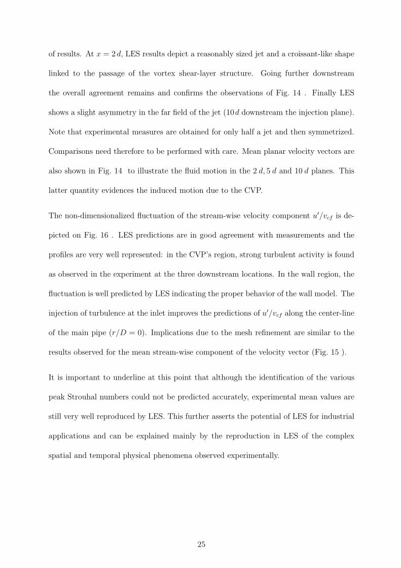
Experimental facility

The experimental rig of 8-JICF is shown on Fig. 1 a. Dimensions and details of the exper-

imental injection system are featured on Fig. 1 b. Full optical access allows detailed anal-

yses of the various flow phenomena. Experimental data consists of LDA (Laser Doppler

Anemometry) , PIV (Particle Image Velocimetry) and PLIF (Planar Laser-Induced Flu-

orescence) fields taken at various cross-stream locations in the main pipe. Point-wise

hot-wire anemometry measurements supplement the data set and are used for temporal

assessments of the main flow structures. Main-pipe inlet velocity profiles measured with

LDA complete the database.

Accuracy of the measured data is ensured through in depth cross validations of the various

diagnostics utilized. Experimental uncertainties are this way limited and clearly identified.

Access to the experimental data is made available through inquiry to the MOLECULES

4

work-package leader, C. Berat ‡, and official consent of all project partners.

Numerical simulations

Turbulent flows are known to contain large ranges of scales.14,27,28 These scales, although

not clearly defined mathematically, have been repeatedly evidenced in experimental mea-

surements or Direct Numerical Simulations (DNS) and LES.29−31 The large scale phe-

nomena are usually associated with vortical structures whose dimensions are of the order

of the domain size. The evolution of these scales is governed by the geometry of the

combustion chamber and they carry most of the turbulent kinetic energy. The smaller

scales have on the other hand a relatively short range of influence and are believed to

behave in a more universal way. Contrary to RANS where all scales need to be modeled,

LES filters out the small universal scales and aims at simulating only the dynamics of the

large scales. The modeling is eased thanks to the universality of the physics governing

the small scales. It yields an approach which is flexible and well suited to simulate cases

encountered in the industry where large scale phenomena are crucial.

Governing equations

LES involves the spatial filtering operation:32

f(x, t) =

∫ +∞

−∞

f(x′, t) G(x′,x) dx′, (1)

‡Turbomeca, Avenue du President Szydlowski, 64511 Bordes, France.

5

where G denotes the filter function and f(x, t) is the filtered value of the variable f(x, t).

We consider spatially and temporally invariant and localized filter functions,32 thus G(x′,x) ≡

G(x′−x) with properties,32,33 G(x) = G(−x) and∫ +∞

−∞G(x)dx = 1. In the mathematical

description of compressible turbulent flows with species transport, the primary variables

are the density ρ(x, t), the velocity vector ui(x, t), the total energy E(x, t) ≡ es +1/2uiui,

and the mass fraction of species α, Yα(x, t). The application of the filtering operation to

the instantaneous transport equations yields:5

∂ρ

∂t+

∂

∂xi

(ρ ui) = 0,

∂

∂t(ρ uj) +

∂

∂xi(ρ ui uj) = −

∂p

∂xj+

∂τ jk

∂xk−

∂

∂xi(ρ Tij),

∂

∂t(ρ E) +

∂

∂xi(ρ ui E) = −

∂qj

∂xj+

∂

∂xj[(τij − p δij) ui] −

∂

∂xj(ρ Qj) −

∂

∂xj(ρ Tijui),

∂

∂t(ρ Yα) +

∂

∂xi(ρ ui Yα) = −

∂Jα

i

∂xi−

∂

∂xi(ρ F α

i ). (2)

In (2), one uses the Favre filtered variable,34 f = ρ f/ρ. The fluid follows the ideal gas

law, p = ρRT and es =∫ T

0Cp dT − p/ρ, where es is the sensible energy, T stands for the

temperature and Cp is the fluid heat capacity at constant pressure. The viscous stress

tensor, the heat diffusion vector and the molecular transport of the passive scalar read

respectively:

τij = µ

(∂ui

∂xj+

∂uj

∂xi

)−

2

3µ

∂uk

∂xkδij, qi = −λ

∂T

∂xi, Jα

i = −ρDα ∂Yα

∂xi. (3)

In (3), µ is the fluid viscosity following Sutherland’s law, λ the heat diffusion coefficient

following Fourier’s law, and Dα the species α diffusion coefficient (note that summation

over repeated indices does not apply to Greek symbols). Variations of the molecular

coefficients resulting from the unresolved fluctuations are neglected hereinafter so that the

6

various expressions for the molecular coefficients become only a function of the filtered

field.

The Tij, QiandFi terms correspond to the so-called Sub-Grid Scale (SGS).10,35 The un-

resolved SGS stress tensor Tij , requires a sub-grid turbulence model. Introducing the

concept of SGS turbulent viscosity most models read:36

Tij = (uiuj − ui uj) = −2 νt Sij +1

3Tkk δij , (4)

with,

Sij =1

2

(∂ui

∂xj+

∂uj

∂xi

)−

1

3

∂uk

∂xkδij. (5)

In (4) & (5), Sij is the resolved strain tensor and νt is the SGS turbulent viscosity. The

WALE model37 (Wall Adapting Local Eddy-viscosity) expresses νt as:

νt = (Cw4)2(sd

ijsdij)

3/2

(SijSij)5/2+(sdijs

dij)

5/4with sd

ij =1

2(g2

ij + g2ji) −

1

3g2

kk δij . (6)

In (6), 4 denotes the filter characteristic length and is approximated by the cubic-root of

the cell volume, Cw is the model constant (Cw = 0.55) and gij = ∂ui/∂xj is the resolved

velocity gradient.

The SGS energy flux Qi = Cp (T ui − T ui) and the SGS scalar flux F αi = (uiYα − ui Yα)

are respectively modeled by use of the eddy diffusivity concept with a turbulent Prandtl

number Prt = 0.9 so that κt = νt Cp/Prt and species SGS turbulent diffusivity Dαt =

7

νt/Scαt where Scα

t is the turbulent Schmidt number (Scαt = 0.7 for all α):

Qi = −κt∂T

∂xiand F α

i = −Dαt

∂Yα

∂xi. (7)

Note that T is the modified filtered temperature and satisfies the modified filtered state

equation,30,38−40 p = ρR T . Although the performances of the closures could be improved

through the use of a dynamic formulation,30,31,41−43 they are sufficient to investigate the

present configuration.

In the context of industry-like configurations the treatment of the wall turbulent boundary

layer needs specific attention. With high Reynolds number flow (here Re = 168, 000), the

turbulent boundary layer is thin compared to the length scales of the computational

domain. To ensure a proper physical behavior of the near-wall solution in the context of

LES two approaches exist. The ”resolved LES” requires a complete analysis of the grid

resolution. With this approach, the inner-layer wall motions (essentially dominated by the

quasi stream-wise vortices) must be sufficiently resolved; the filter and grid spacing must

be of the order of δν (δν is the length-scale of the viscous wall region). It can be estimated

that the number of grid nodes required increases as Re1.76 in the inner-wall region of

the flow. For the outer-layer, which contains the large eddy scales, the grid resolution

must resolve the turbulent kinetic energy and usually scales as Re0.4. The ”resolved

LES” approach usually implies too large computational costs for its direct application

to high Reynolds number problems.44 The second approach known as the ”approximate

boundary condition” methodology proposes to model the whole wall region. Numerous

simplifications for the near-wall LES behavior have been investigated.45−47 In this work,

the log law model48−50 is assumed and the wall stresses are modeled so as to mimic the

wall effects on the global flow behavior. Note that in the implementation of this approach

8

the wall boundary conditions use a non-zero velocity at the wall, which is determined

locally using the log law and the information on the grid points directly above the wall

nodes. Corrections on the temperature profile follow the same approach.

General description of the code

All computations are performed with a compressible Navier-Stokes code simulating un-

steady flows on structured, unstructured and hybrid grids (cf. http://www.cerfacs.fr).

For the prediction of unsteady turbulence, different LES sub-grid scale models have been

developed including the WALE model37, Eq. (6). The numerical discretization of the

governing equations, Eqs. (2-7), uses a cell-vertex method51,52 and the discrete values

of the conserved variables are stored at the cell vertices (or grid nodes). Despite the

possible use of a numerical scheme offering third-order spatial and temporal accuracies

(TTGC scheme53), computations presented in this work are obtained with a second-order

Lax-Wendroff scheme.

Simulations

Experiments for 8-JICF were performed for two values of the jet-to-mainstream momen-

tum flux ratio, J defined by:

J =ρjetv

2jet

ρcfv2cf

, (8)

a low impulse case (J = 4) and a large one (J = 16). Both cases have been investigated

with LES. For clarity, only the predictions obtained for J = 16 are presented in this

work (similar topological behavior was obtained for the case J = 4). The flow Reynolds

9

number, based on the main-stream bulk velocity (vcf) and the main duct diameter (D),

equals 168, 000 for all cases. It ensures high level of mixing and limited effects of the

turbulent boundary layer. The jet Reynolds number based upon the jet diameter (d) and

jet bulk velocity (vjet) equals 20, 500 and 41, 000 for J = 4 and J = 16 respectively. Note

that due to the use of equal density fluids, the jet-to-mainstream momentum flux ratio

J is equivalent to the square of the velocity ratio, R = vjet/vcf . This flow parameter is

hereinafter preferred to identify each case (i.e. R = 4 for J = 16 and R = 2 for J = 4).

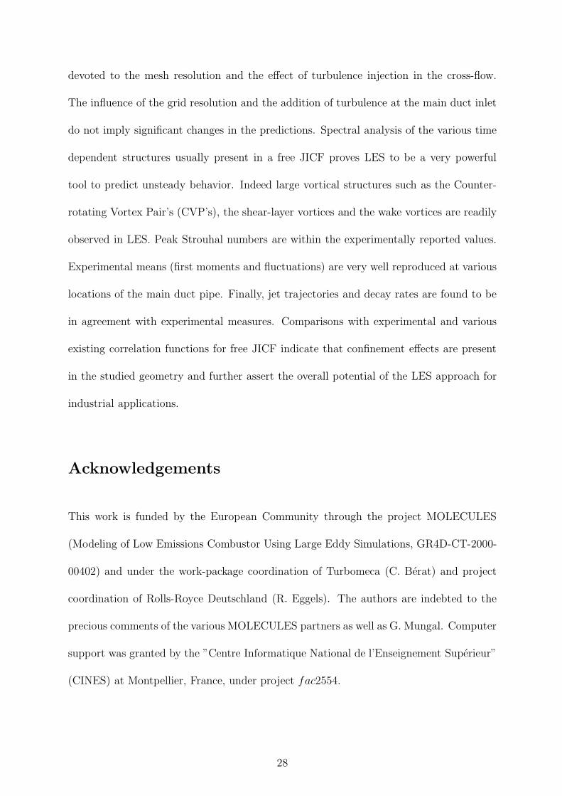
Computational domain

Figure 2 illustrates the computational domain retained for the 8-JICF experimental set-

up shown on Fig. 1 . The length of the main pipe is 138.3 mm for a diameter of 100

mm. The jet inlet sections are located 18.3 mm downstream the main pipe inlet and 120

mm upstream the pipe outlet section. All jets are positioned 45 degrees (π/4 radians)

apart around the duct circumference. To reduce mesh size and computational cost, the

injection system is modeled in LES by a straight injection system prolonged by a circular

duct with dimensions identical to the one found in the experiment. The modeled section

is circular (see on Fig. 2 b) with a contraction ratio of β = 0.811. The jet inlet section

has a diameter of 6.92 mm and 6.1 mm at the junction with the main pipe. The aim of

this modification is to allow a proper acoustic treatment of the jet injection section in the

main tube.24−26

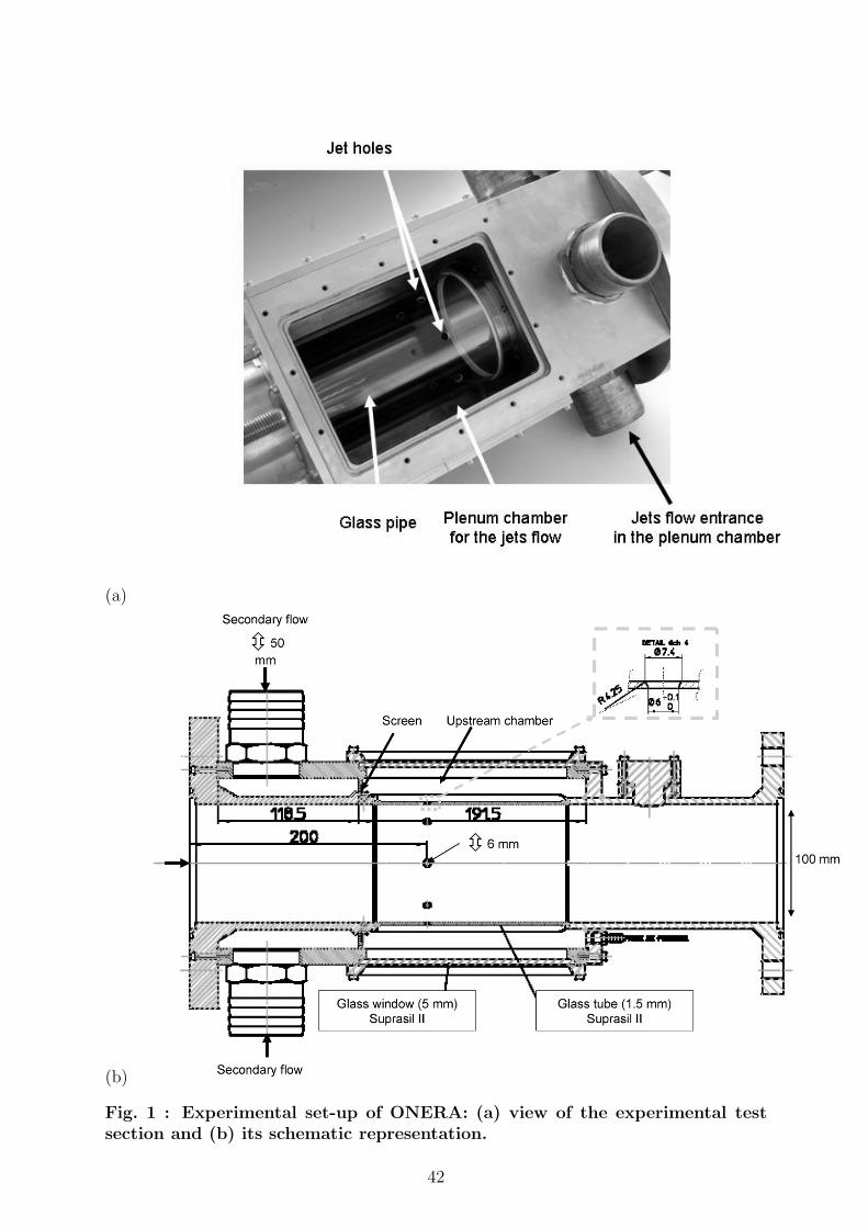
The grid is fully unstructured and composed of tetrahedra. To control the total number of

cells and reduce computational cost, mesh refinement is enforced where necessary. More

specifically, injection areas, wall regions and jet trajectories must be sufficiently resolved

to capture the appropriate range of length-scales. To facilitate refinement along the jet

10

trajectory, a correlation function is used as a guideline within the computational domain.

The guiding trajectory follows the expression for a single JICF54 with low velocity ratio,

R,

x

d=

(2.351 +

4

R

)0.385(1

R

)2.6(y

d

)2.6

. (9)

In Eq. (9), x is the stream-wise direction, y the wall normal direction and d the jet diam-

eter. For the grid generation, the velocity ratio, R in Eq. (9), is taken to 4 irrespectively

of the case simulated. Although several laws for JICF trajectories are proposed in the

literature, the dependency of the LES predictions on the correlation function to be used

is not addressed in this work.

The two meshes as seen on Fig. 3 are used for all the LES (i.e. R = 2 and R = 4).

A coarse mesh M1 and a finer one M2 allow a clear assessment of the grid resolution

(Table 1) and its impact on the time averaged LES predictions. The minimum cell size

is located in the region where the jet meets the main-stream flow and is the same for all

jets. Computational effort corresponding to an increase of resolution from meshes M1 to

M2 yields a factor of 1.625 in the total CPU time. §

Boundary and initial conditions

Dealing with a fully compressible flow solver, special attention must be paid to the treat-

ment of acoustics through the Boundary Conditions (BC). Acoustic waves can be gen-

erated through artificial transient phenomena due to the approximated initial solution

and/or the wrong treatment of the BC’s. For clarity, the set of BC’s used in the LES is

listed in Table 2. They are based on the method of characteristics.55−57 All inlet condi-

§as obtained on 32 O3800 processors of a SGI Power Challenge hosted by CINES (one flow-throughtime taking approximately 8 CPU hours on mesh M1).

11

tions operate with the same type of BC (Table 2). For an inlet, the three components of

the velocity vector, the temperature and species mass fractions are imposed to the desired

values through a relaxing parameter.56 When this coefficient equals zero the BC is acous-

tically non-reflective: exiting acoustic waves leave the domain freely and no component

is re-injected in the computational domain. When the coefficient is non-zero the exiting

acoustic wave is partially reflected and remains within the region of computation. Fur-

thermore zero relaxing coefficient may result in drifting mean quantities and sufficiently

large relaxation coefficients are needed so that mean values remain close to their target

values.58

Turbulent pipe flow profiles are used to set the jet mean inlet velocity conditions (Patch

B in Fig. 2 ). The resulting bulk velocity respects the mass flux as measured by ONERA.

It should be noted that in the case of a no-slip wall, a zero velocity is imposed at the

wall and the shape of the velocity profile issued at the intersection of the injection system

and the main duct strongly depends on the grid resolution of the jet injection system.

For this reason outlet jet profiles found in LES may not reproduce experimental profiles

at these locations. To diminish the differences and the potential implications on the flow

predictions, no-slip isothermal (T= 300 K) walls are used in the jet injection systems with

an increased grid resolution (Patch E in Fig. 2 ). Other walls (Patch D in Fig. 2 ) follow

the isothermal wall law condition described previously.

At the main duct inlet (Patch A in Fig. 2 ) the values of u, v and w vary in time and

space to reproduce the effect of an incoming turbulent field as observed in the experiment.

The method in constructing the incoming turbulent signal is based on the Random Flow

Generation (RFG) algorithm59−61 itself based on early work.62 The continuously homoge-

neous isotropic incoming field consists of a superposition of harmonic functions (50 modes

12

projected in the three directions) with characteristic length-scales prescribed by the user.

Forcing the flow in such a way considerably accelerates the establishment of fully devel-

oped turbulent flows. It also ensures the presence of coherent perturbations not warranted

when a pure white noise is used. Figure 4 depicts main-stream inlet profiles. All results

are non-dimensionalized by the cross-flow velocity vcf . Experimental measures are added

as symbols. Measurement errors are for the mean field below 1% and around 4% for the

fluctuating components. The actual response of the code with and without ”injection of

turbulence” are respectively represented by the solid lines and the broken lines. All LES

results agree with the measurements. Deviations of the LES fluctuating profiles from the

mean target fluctuating profile imposed at the BC are due to the unsteady nature of the

incoming flow and the partially reflective condition.

The main duct outlet BC (Patch C in Fig. 2 ) simulates a far field state with given

atmospheric conditions. This boundary condition is ”soft”; the in-going wave is computed

as a difference between the LES solution at the boundary nodes and the reference state. A

”relax” coefficient allows to absorb the acoustics making the condition partially reflective.

All relax coefficients used for the LES of 8-JICF are listed in Table 2 and assure low

acoustic impedance of the boundary as verified by a posteriori validation of the incoming

and out-going acoustic signals.58 Finally and to identify the mixing of the jets with the

cross-flow fluid, oxygen issued at the jet air inlet condition is differentiated from the

oxygen of the cross-flow air.

In order to proceed with the integration of the LES governing equations an initial solution

is needed. To diminish computational cost and artificial effects due to the initial guess a

specific methodology is employed. Two steps are followed:

13

1) To achieve an approached solution in a reasonable time delay, the coarse mesh (M1)

is first used to conduct the integration. To avoid spurious behaviors, the initial

velocity is null and tends smoothly to the desired values through the inlet BC’s.

2) The converged solution obtained in 1) is interpolated on the fine mesh (M2) to yield

a new initial condition for proper integration of the LES equations.

Note that each step requires adaptation of the initial conditions toward physical solu-

tions. Memory loss of the initial guesses is assured by allowing the simulation to run for

approximately one flow-through time before starting statistical sampling and analysis of

the LES results.

Results and discussion

Prior to the discussion on the LES and experimental flow topology, a brief introduction

to the single JICF features is given. Jet visualizations of the 8-JICF LES predictions for

the fine grid (M2) and both velocity ratios follow. Vortex shedding frequencies in the near

field region are investigated and gauged against experimental measurements. Then, mean

velocity fields are presented along with a qualitative assessment of the grid resolution and

turbulence injection effects. Finally, one assesses jet trajectories and decay rates.

Flow features

The single JICF configuration is widely used in many technical applications involving gas

turbines, fuel injection, chimneys, etc. Compared to other shear flows (e.g. mixing layer,

free jets) the JICF is the result of the complex three-dimensional interactions between

14

the jet and the cross-flow stream. It displays considerably more complexity with jet-like

behavior in the near field and the far field. The literature proposes numerous works on the

main vortical structures observed in several regions of the single JICF.63−66 Four distinct

vortical structures have been identified (see Fig. 5 ):

1 The jet shear-layer vortices which evolve on the jet column and whose vorticity is

generated at the interface between the jet and the cross-stream. Such structures are

the result of the Kelvin-Helmholtz instabilities of the annular shear-layer.

2 The horseshoe vortex system, which lies on the wall around the jet exit and which is

quite similar to the structures observed for flows around a cylinder wall junction.65

It also has been shown that the horseshoe relates to the shear-layer roll up and the

shedding of vortices in the wake region.

3 The wake structures form downstream the jet column and persist far downstream of

the exit nozzle. The fluid comes from the wall boundary layer and sheds regularly

from the lee-ward side of the jet. They can be detected in the wake region as

ascending vortices. These very complex three-dimensional flow patterns are strongly

influenced by the jet trajectory.

4 The Counter-rotating Vortex Pair (CVP) is the dominant coherent structure of the

JICF. It develops downstream and strongly depends on the boundary layer and

plane wall region. The CVP plays a significant role in the far-field mixing.

In this paragraph, the single jet topology as obtained from the 8-JICF LES is presented

for R = 2 and R = 4 with the help of four identification tools. Only the near-field

region of one JICF out of the 8-JICF configuration is illustrated. It ensures that each

JICF feature is not influenced by the neighboring JICF’s. Figures 6 a and 7 a show iso-

15

surfaces of jet oxygen mass fraction; inner and outer jet boundary layers are defined by

a jet oxygen mass fraction of 0.1. Jet air rapidly mixes with cross-flow fluid to generate

oxygen pockets. Such iso-surfaces indicate that as R increases, the jet integrity is clearly

shortened in space, thus corresponding to enhanced mixing. The differences are asserted

by Figs. 6 b and 7 b where iso-surfaces of low level of pressure are shown. Figures 6 c and

7 c illustrate the Q-criterion. Based upon the second invariant of the velocity gradient

tensor,67 this criterion aims at detecting coherent structures in wall bounded turbulent

flows. Q is directly related to the pressure Laplacian, ∇2p = 2 ρ Q, for inviscid flows

and can be interpreted as the source term of pressure in the Navier-Stokes equations.

On Figs. 6 d and 7 d, the strong velocity gradients present near the wall prevent a clear

identification of large scale features through the stream-wise component of the vorticity

vector. This drawback is circumvented with the help of the Q-criterion (Figs. 6 c and 7 c)

which allows to identify structures already illustrated with the iso-surfaces of jet oxygen

mass fraction.

All criteria show the jet column to deviate while it penetrates the cross-flow. This pro-

nounced feature of the JICF (see Fig. 5 ) is present in the 8-JICF configuration. Shear-

layer vortices can also be noticed for both velocity ratios. Traces of the CVP are also

evidenced in the 8-JICF set-up. The major difference observed between case R = 4 and

case R = 2 is the penetration angle of each individual JICF and its transition toward a

fully turbulent state. Strong similarities can however be found between the two cases as

reported in previous works on JICF. Based on these observations only R = 4 results are

presented afterward.

16

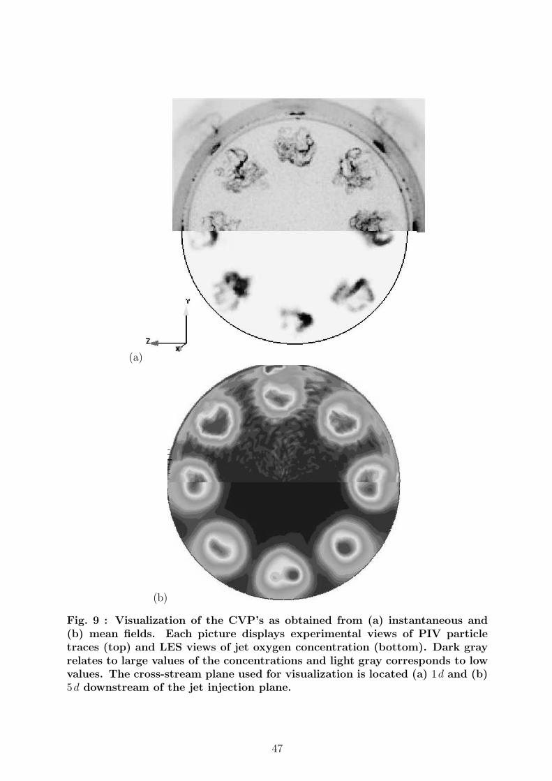
The Counter-rotating Vortex Pair (CVP)

The CVP is a well known feature of the JICF configuration.64,68 This coherent structure

persists and keeps evolving even in the far field region of the flow. It appears in steady

and unsteady flow solutions and does not dependent on the velocity ratio R and the flow

Reynolds number Re. The CVP takes on an oval shape composed of two kidney shaped

counter-rotating vortices.

Figure 8 shows the CVP as observed in the 8-JICF LES predictions for one of the

eight JICF. The normalized stream-wise component of the vorticity vector, Ωx, is shown

at a) x = 1d and b) x = 2d. Dark grey iso-lines correspond to clockwise rotations

while light grey iso-lines identify counter-clockwise rotations. The normalization of Ωx by

the planar maximum of |Ωx0| within the CVP (outside of the wall region) is performed

so as to illustrated the downstream evolution of the CVP. Through this quantity the

kidney-like structures are clearly observed in the LES predictions. The decay of the

structure with the downstream direction is confirmed by LES (Figs. 8 a-b). Built-in

diffusive as well as dissipative forces of the system imply a decrease in the maximum of

vorticity as the jet expands. It is to be noted that the rotation of the two kidney-like

structures induces creation of vorticity in the near-wall region and also decreases with the

downstream direction.

Comparisons of the jet oxygen concentration given by an instantaneous LES solution

with PIV particle traces in the CVP region (Fig. 9 a) suggest that LES predictions

and measurements do not necessarily depict well defined and coherent structures at all

instants and for all jets of 8-JICF. Gross agreement can be found but no clear small or

large scale pattern is identified in any jet. Finally, Fig. 9 a underlines the unsteadiness

17

of the flow evidenced through the asymmetries in the particle traces and the jet oxygen

concentration. These asymmetries are not clearly evidenced by the averaged results (Fig. 9

b). The qualitative good agreement between LES and measurements as illustrated in

Fig. 9 highlights the clear potential of LES for industry-like computations.

Statistical analysis

Instantaneous visualization of the LES predictions reveals the possibilities of the approach

in predicting highly complex flows. Further analysis is however necessary to clearly assess

LES for industrial applications. To do so, comparisons of the statistically averaged LES

fields and corresponding experimental data are presented in this section. A frequency

analysis of the various JICF structures identified previously is exposed, followed by sta-

tistical moments. Finally, mixing of the jet air with the main-flow is evaluated and gauged

against existing correlation functions. It is of interest to underline at this point that LES

animations point out that the instantaneous realizations of the JICF may deviate from

their theoretical trajectory. The appearance of a weak coupling between neighboring jets

is to be suspected in 8-JICF. Under these circumstances an independent treatment of all

the JICF should be interpreted with care even if the time scales of the coupling appeared

to be very long.

Vortex shedding frequencies

Vortex shedding frequencies are of clear interest to the JICF users; large vortex structures

can have a substantial impact on the mixing of the jets, which is one of the primary aim

of the gas turbine industrial use of JICF’s. In the experimental investigations, Fourier-

spectral analysis of velocity signals (hot-wire anemometry) has been performed in two

18

distinct regions: the wake and the jet shear-layer. Probe’s locations have been determined

based on visual investigations of the flow.

This paragraph presents the frequency acquisition method conducted on the numerical

simulations. Wake and jet shear-layer vortices are studied at several probe locations where

pronounced harmonics are found experimentally. In order to obtain a proper convergence

of the spectral analysis, two hypotheses are needed for LES : first, the axi-symmetry of

the flow is assumed although it has been pointed out that all jet penetrations are not

strictly identical and independent. Second, traveling in the downstream direction along

the jet column, structures are supposed to be persistent and vortex shedding frequency is

assumed to be equivalent for different probe locations in the regions of interest and prior

to potential vortex pairings. Under these two assumptions, averaging of the individual

Fourier-spectrum is performed and compared to the measurements. The duration of the

time series equals 37 ms (i.e. 6.7 convective times) and the sampling is performed at 6, 000

Hz. These time-span and sampling rate enable to capture most of the flow information.

For the wake region, the analysis is based on the time series of the stream-wise component

of the velocity vector, u(x, t) obtained on the fine grid, M2. The same approach is used in

the vortex shear-layer with u(x, t) being sampled. The respective spectra are presented

in terms of Strouhal numbers, St = f Lref/Uref , where f is the frequency domain (in

s−1), Uref and Lref are the reference velocity and reference length. Reference values need

to be adjusted depending on the phenomena investigated. In this study, two regions

are investigated: the wake region for which we take Uref = vcf and Lref = d yielding

Stvcf= f d/vcf , and the jet shear-layer for which we have Uref = vjet and Lref = d

yielding Stvjet= f d/vjet.

The wake region is discussed first. Few references are found on this subject in JICF’s

19

literature. Characteristic Strouhal numbers found for the Karman street behind a circular

cylinder vary around Stvcf= 0.21. JICF wake vortices were studied with the use of the

smoke-wire technique63 for several velocity ratios, R. In the mentioned work, a degree

of repeatability is found for the case R = 4 and varying cross-flow Reynolds numbers

ranging from 3, 800 to 11, 400. The experimental Strouhal number equals 0.13 for R = 4.

Transitions to larger values occur around R = 3 and R = 6. In another experiment,70

the problem is investigated for R ranging from 2 to 8 and a fixed cross-flow Reynolds

equal to 8, 000. The probe is located 2.7 jet diameters downstream the injection point

and Stvcf= 0.15. In 8-JICF experiments, the velocity probe is placed 6 mm from the

wall and 12 mm downstream of the jet axis. Treatment of the unsteady LES results is

obtained with five probes placed in the wake region behind the injection zone and 2 mm

apart (Fig. 10 ).

Vortex shedding frequencies are computed for all of the eight JICF present in the flow (i.e.

in all eight wake regions). Fast Fourier transforms obtained from the forty points, are

averaged and the corresponding LES Fourier-spectrum is shown on Fig. 11 a. Experimen-

tal results are illustrated on Fig. 11 b. Broken line represents fast Fourier transforms of

the stream-wise component of the velocity vector u(x, t), and continuous line represents a

smoothed signal (after averaging over all the realizations). LES predictions depict regular

vortex shedding at one pronounced frequency corresponding to a Strouhal number of 0.18.

Experiment yields a lower Strouhal number equal to 0.11 (Fig. 11 b).

Vortex shedding frequencies of jet shear-layer structures have received more attention from

researchers especially for acoustically excited transverse jets. Concerning unforced JICF,

recent experiments65 in both water and air suggest that periodic vortex ring roll-ups from

the nozzle appear with a Strouhal number equal to 0.295. Another experiment points out

20

the importance of the probe location.71 The corresponding work reports different Strouhal

number for a hot-wire probe positioned from approximately 1 to 1.5 jet diameters above

the upstream edge of the jet exit. According to their observations, higher harmonics

appear with increasing value of the cross-stream speed while keeping the velocity ratio

constant (R = 4): Stvjet= 0.721 with vjet = 4.8 m/s and Stvjet

= 0.828 for vjet = 8 m/s.

The impact of the downstream location of the measuring point was also addressed.72

To do so, the authors register velocity signals at three positions in the jet shear-layer

of a JICF with cross-flow Reynolds number of 27, 500 and a velocity ratio of 6. The

reported Strouhal numbers are found to decrease with increasing downstream position.

Finally, Direct Numerical Simulations (DNS) assess the influence of the wall boundary

layer.73 The numerical experiments are performed for different velocity ratios and one

non-dimensionalized boundary layer thickness δBL/d = 0.5. For R = 5.4 their finding is:

Stvjet= 0.545.

Figure 12 shows the three probe locations used to analyze LES predictions in the jet

shear-layer region. The probes are positioned close to the upstream edge of the jet shear-

layer to help discern the large structure frequencies. In the experiment, the probe is

placed 6 mm from the wall and 3 mm upstream of the jet axis.

LES predictions are compared against experimental data on Fig. 13 . Spectrum’s shape

is qualitatively well reproduced. The high response observed at low frequencies probably

corresponds to the CVP’s formation. For both cases, the spectra seem to be masked by

broad-band behavior with no discernible dynamics in the range 0 < Stvjet< 0.07. This can

be explained by the fact that probes are located slightly inside the jet and reveal internal

details of the CVP’s structure. For 0.07 < Stvjet< 0.27, the LES spectrum remains stable

and reveals a small peak around a Strouhal number value of 0.24. The same general

21

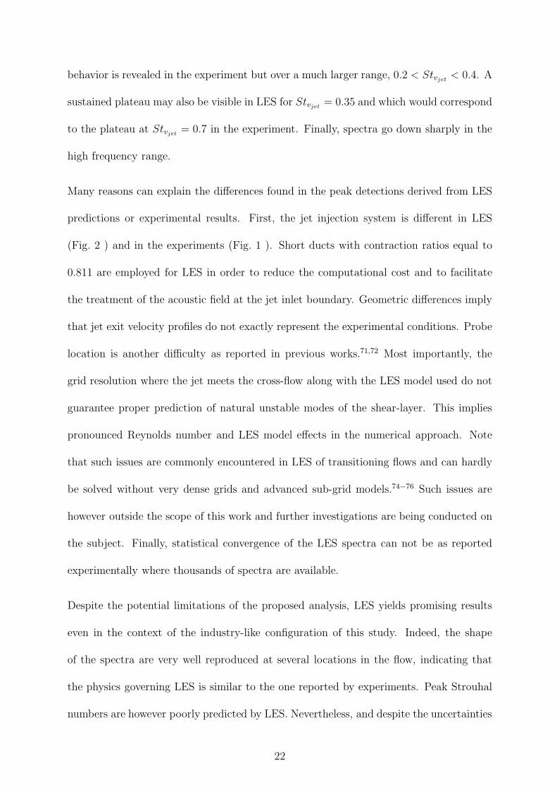
behavior is revealed in the experiment but over a much larger range, 0.2 < Stvjet< 0.4. A

sustained plateau may also be visible in LES for Stvjet= 0.35 and which would correspond

to the plateau at Stvjet= 0.7 in the experiment. Finally, spectra go down sharply in the

high frequency range.

Many reasons can explain the differences found in the peak detections derived from LES

predictions or experimental results. First, the jet injection system is different in LES

(Fig. 2 ) and in the experiments (Fig. 1 ). Short ducts with contraction ratios equal to

0.811 are employed for LES in order to reduce the computational cost and to facilitate

the treatment of the acoustic field at the jet inlet boundary. Geometric differences imply

that jet exit velocity profiles do not exactly represent the experimental conditions. Probe

location is another difficulty as reported in previous works.71,72 Most importantly, the

grid resolution where the jet meets the cross-flow along with the LES model used do not

guarantee proper prediction of natural unstable modes of the shear-layer. This implies

pronounced Reynolds number and LES model effects in the numerical approach. Note

that such issues are commonly encountered in LES of transitioning flows and can hardly

be solved without very dense grids and advanced sub-grid models.74−76 Such issues are

however outside the scope of this work and further investigations are being conducted on

the subject. Finally, statistical convergence of the LES spectra can not be as reported

experimentally where thousands of spectra are available.

Despite the potential limitations of the proposed analysis, LES yields promising results

even in the context of the industry-like configuration of this study. Indeed, the shape

of the spectra are very well reproduced at several locations in the flow, indicating that

the physics governing LES is similar to the one reported by experiments. Peak Strouhal

numbers are however poorly predicted by LES. Nevertheless, and despite the uncertainties

22

associated with the flow configuration and the numerical approach, LES predictions are

very encouraging.

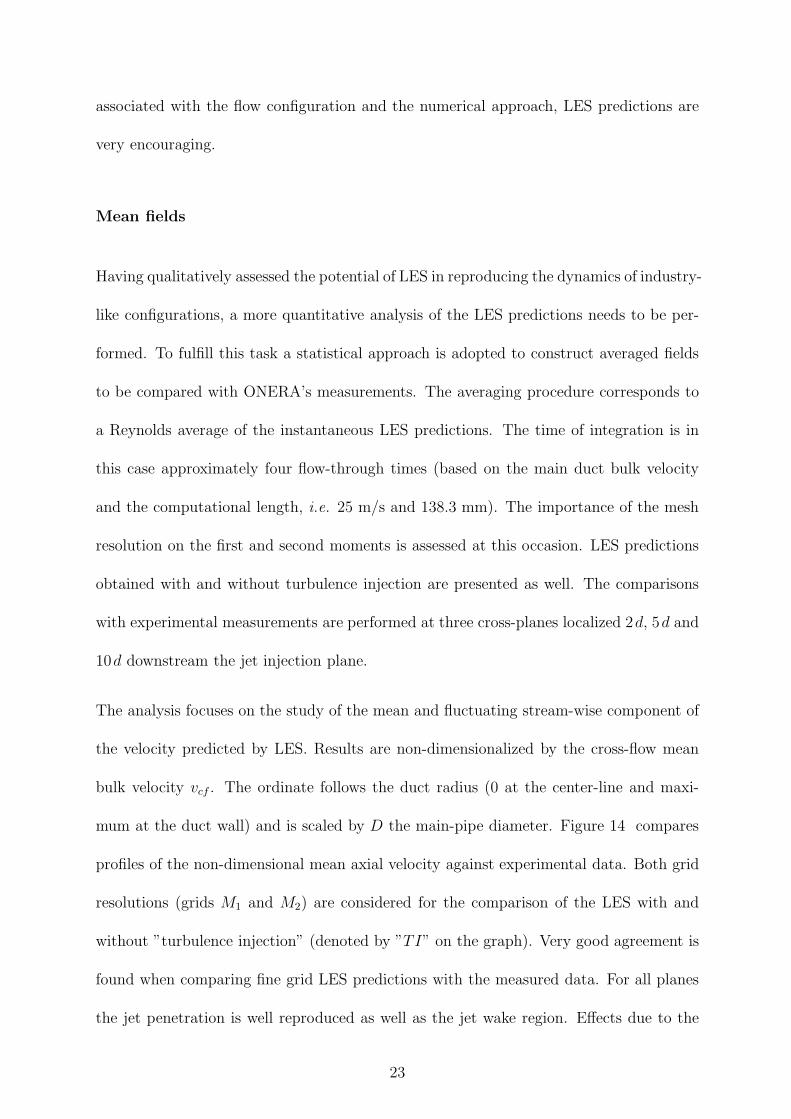
Mean fields

Having qualitatively assessed the potential of LES in reproducing the dynamics of industry-

like configurations, a more quantitative analysis of the LES predictions needs to be per-

formed. To fulfill this task a statistical approach is adopted to construct averaged fields

to be compared with ONERA’s measurements. The averaging procedure corresponds to

a Reynolds average of the instantaneous LES predictions. The time of integration is in

this case approximately four flow-through times (based on the main duct bulk velocity

and the computational length, i.e. 25 m/s and 138.3 mm). The importance of the mesh

resolution on the first and second moments is assessed at this occasion. LES predictions

obtained with and without turbulence injection are presented as well. The comparisons

with experimental measurements are performed at three cross-planes localized 2d, 5d and

10d downstream the jet injection plane.

The analysis focuses on the study of the mean and fluctuating stream-wise component of

the velocity predicted by LES. Results are non-dimensionalized by the cross-flow mean

bulk velocity vcf . The ordinate follows the duct radius (0 at the center-line and maxi-

mum at the duct wall) and is scaled by D the main-pipe diameter. Figure 14 compares

profiles of the non-dimensional mean axial velocity against experimental data. Both grid

resolutions (grids M1 and M2) are considered for the comparison of the LES with and

without ”turbulence injection” (denoted by ”TI” on the graph). Very good agreement is

found when comparing fine grid LES predictions with the measured data. For all planes

the jet penetration is well reproduced as well as the jet wake region. Effects due to the

23

increased mesh resolution in the jet near field are readily observed and result from three

highly coupled phenomena. First, local increase of the mesh resolution allows one to en-

rich the LES flow solution with smaller and better resolved small scale structures. The

downstream JICF region is in turn ”more turbulent” and the large scale energy content is

better represented. Second, associated with this grid refinement, is also a less dissipative

LES. Improved levels of dissipation originate from a more efficient application of the LES

model. The flow structures influenced by the model are closer to the required assumption

for the use of the SGS model, i.e. local isotropy. Third and last, smaller cell volumes

usually go with decreased dissipative effects induced by the numerical scheme itself. Con-

sequently and as observed in Fig. 14 , the mean stream-wise profiles are expected to be

sharper (less diffused) in regions of improved energetic content, i.e. 2d and 5d. These

results illustrate the necessity to properly resolve regions of importance for LES to yield

good quality predictions. Iterative approach with adaptation of the local mesh resolution

(as performed here) may therefore be required when no clear information can be inferred

for the flow to be simulated. Finally, when turbulence injection (TI) is used, no signif-

icant change is observed when compared to other LES predictions. The intensity of the

perturbations at the main inlet probably does not influence such turbulent shear flows.

The importance of the cross-flow turbulence is in this context not clear even though it

is well known that such an approach may significantly improve the prediction in more

academic configurations.

Figure 15 displays the mean axial component of the velocity vector for one eighth of the

cross-sectional planes located at 2d, 5d and 10d. Each LES field shown in the figure is

time-averaged over two flow-through times and spatially averaged over the eight jets to

yield one section as obtained in the experiment. The color-map is identical for both set

24

of results. At x = 2d, LES results depict a reasonably sized jet and a croissant-like shape

linked to the passage of the vortex shear-layer structure. Going further downstream

the overall agreement remains and confirms the observations of Fig. 14 . Finally LES

shows a slight asymmetry in the far field of the jet (10d downstream the injection plane).

Note that experimental measures are obtained for only half a jet and then symmetrized.

Comparisons need therefore to be performed with care. Mean planar velocity vectors are

also shown in Fig. 14 to illustrate the fluid motion in the 2 d, 5 d and 10 d planes. This

latter quantity evidences the induced motion due to the CVP.

The non-dimensionalized fluctuation of the stream-wise velocity component u′/vcf is de-

picted on Fig. 16 . LES predictions are in good agreement with measurements and the

profiles are very well represented: in the CVP’s region, strong turbulent activity is found

as observed in the experiment at the three downstream locations. In the wall region, the

fluctuation is well predicted by LES indicating the proper behavior of the wall model. The

injection of turbulence at the inlet improves the predictions of u′/vcf along the center-line

of the main pipe (r/D = 0). Implications due to the mesh refinement are similar to the

results observed for the mean stream-wise component of the velocity vector (Fig. 15 ).

It is important to underline at this point that although the identification of the various

peak Strouhal numbers could not be predicted accurately, experimental mean values are

still very well reproduced by LES. This further asserts the potential of LES for industrial

applications and can be explained mainly by the reproduction in LES of the complex

spatial and temporal physical phenomena observed experimentally.

25

Jet trajectories and decay rates

JICF jet trajectories have received a lot of attention from researchers as well as from

the industry. Often based on the locus of the maximum stream-wise component of the

velocity vector, the jet path can also be defined as the locus of the maximum jet scalar

concentration in this same plane. Many experimental and theoretical works on free JICF’s

indicate that the jet path can be expressed in self-similar variables for a large range of

jet-to-mainstream momentum flux ratio (at least for free JICF). Some of the experimental

correlations resulting from these previous works are given in Table 3.

LES results are gauged for both definitions against free JICF’s experimental correlations

as obtained for a velocity ratio of R = 4. Figures 17 a-b respectively show jet paths in

self-similar coordinates based on the stream-wise component of the velocity vector and

the scalar concentration maximum as functions of the non-dimensionalized downstream

directions. Agreement with experimental measurements on 8-JICF is very good and

validates the LES results. When compared with analytical expressions, the present results

are found to under-predict the proposed correlation functions over the entire length of the

domain. Such results highlight the impact of the geometric differences between 8-JICF

and a single free JICF. Confinement is expected to play a determining role in the latter

while deliberately nonexistent in the former. Focusing on the criterion constructed from

the velocity field (Fig. 17 a), the initial jet deflection observed experimentally in the range

0 < x/d < 5 and the downstream region x/d > 10 are very well replicated for both mesh

resolutions (grids M1 and M2), with and without turbulence injection (TI). LES and

measures for 8-JICF are closer to the third and fifth correlation function.77 For the jet

oxygen maximum concentration (Fig. 17 b) jet penetration is found to be closer to the first

expression78 for the scalar and LES reproduce the correlation in the near field region. The

26

mesh resolution and the turbulence injection do not seem to influence the jet trajectory.

Figures 18 a-b respectively display the decays of the maximum stream-wise component

of velocity and the maximum jet oxygen scalar concentration along the respective tra-

jectories shown on Fig. 17 . The abscissa corresponds to the distance traveled along the

jet trajectory from the injection point (denoted here by s). The decays are presented in

a non-dimensional form as indicated in the literature.68,79 Figure 18 suggests power law

decays as observed in free JICF’s. In the near field region, ln(s/Rd) < 1, the maximum of

velocity decreases to a −1 power as encountered for free turbulent jets. For ln(s/R d) > 1

(i.e. s ≈ 15 d), a transition occurs and the decay rate tends toward the value of −2/3

as reported for free JICF.80,81 These changes in slope are often related to the CVP which

increases the rate of mixing and the decay rate of the maximum value of the stream-wise

velocity component. Fig. 18 b corroborates the previous findings, especially for the case

performed with turbulence injection. The near field jet-like decay is less pronounced and

mixing seems accentuated when LES is closely analyzed. Modeling effects would need to

be assessed to further validate the approach. The influence of the grid resolution is not

significant in predicting the velocity and scalar concentration decay rates.

Conclusions

This work assesses the potential of the Large Eddy Simulations (LES) approach in the

context of an industry-like configuration. The study focuses on a typical dilution zone

in gas-turbine geometries. More specifically LES are performed for eight isothermal Jets

In Cross-Flow (JICF) issuing radially in a round pipe. Experimental measurements and

detailed diagnostics allow a clear assessment of the LES predictions. Special attention is

27

devoted to the mesh resolution and the effect of turbulence injection in the cross-flow.

The influence of the grid resolution and the addition of turbulence at the main duct inlet

do not imply significant changes in the predictions. Spectral analysis of the various time

dependent structures usually present in a free JICF proves LES to be a very powerful

tool to predict unsteady behavior. Indeed large vortical structures such as the Counter-

rotating Vortex Pair’s (CVP’s), the shear-layer vortices and the wake vortices are readily

observed in LES. Peak Strouhal numbers are within the experimentally reported values.

Experimental means (first moments and fluctuations) are very well reproduced at various

locations of the main duct pipe. Finally, jet trajectories and decay rates are found to be

in agreement with experimental measures. Comparisons with experimental and various

existing correlation functions for free JICF indicate that confinement effects are present

in the studied geometry and further assert the overall potential of the LES approach for

industrial applications.

Acknowledgements

This work is funded by the European Community through the project MOLECULES

(Modeling of Low Emissions Combustor Using Large Eddy Simulations, GR4D-CT-2000-

00402) and under the work-package coordination of Turbomeca (C. Berat) and project

coordination of Rolls-Royce Deutschland (R. Eggels). The authors are indebted to the

precious comments of the various MOLECULES partners as well as G. Mungal. Computer

support was granted by the ”Centre Informatique National de l’Enseignement Superieur”

(CINES) at Montpellier, France, under project fac2554.

28

References

1Rayleigh, L., ”The explanation of certain acoustic phenomena,” Nature, Vol. 18, 1878,

pp. 319-321.

2Putnam, A. A., ”Combustion driven oscillations in industry,” American Elsevier, 1971.

3Strahle, W., ”Combustion noise,” Energy and Combustion Science, Vol. 4, 1978, pp.

157-176.

4Williams, F. A., Combustion theory, New-York, Benjamin Cummings, 1985.

5Poinsot, T. and Veynante, D., ”Theorical and Numerical Combustion,” R. T. Edwards,

2001.

6Ferziger, J. H., ”Large eddy simulations of turbulent flows,” AIAA Journal, Vol. 15, No.

9, 1977, pp. 1261-1267.

7Lesieur, M. and Metais, O., ”New trends in large-eddy simulations of turbulence,” An-

nual Review Fluid Mechanics, Vol. 28, 1996, pp. 42-82.

8Mason, P. J., ”Large-eddy simulation: A critical review of the technique,” Quaterly Jour-

nal of the Royal Meteorological Society, Vol. 120, 1994, pp. 1-26.

9Rogallo, R. S. and Moin, P., ”Numerical simulation of turbulent flows,” Annual Review

Fluid Mechanics, Vol. 16, 1984, pp. 99-137.

10Sagaut, P., Large Eddy Simulation for incompressible flows, New York, Springer, 2001.

11Launder, B. E. and Spalding, D. B., Mathematical models of turbulence, London, Aca-

demic Press, 1972.

12Pope, S. B., Turbulent Flows, Cambridge, UK, Cambridge University Press, 2000.

13Chassaing, P., Turbulence en Mecanique des fluides. Analyse du phenomene en vue de

sa modelisation a l’usage de l’ingenieur, Toulouse, Polytech, 2000.

14Tennekes, H. and Lumley, J. L., ”A First Course in Turbulence,” The MIT press, 1972.

29

15Chiu S.H., Roth K.R., Margason R.J. and Jin Tso, ”A numerical investigation of a sub-

sonic jet in cross flow,” In Computational and Experimental Assessment of Jets in Cross

Flow, CP-534, AGARD, November, 1993.

16Alvarez J., Jones W.P. and Seoud R., ”Predictions of momentum and scalar fields in a

jet in cross flow using first and second order turbulence closures,” In Computational and

Experimental Assessment of Jets in Cross Flow, CP-534, AGARD, November, 1993.

17Claus R.W. and Wanka S.P., ”Multigrid calculations of a jet in crossflow,” J. Propulsion

Power, 8, 1992, pp. 423-431.

18Kim S.W. and Benson T.J., ”Calculation of a circular jet in crossflow with multiple-

time-scale turbulence model,” Intl. J. Heat Mass Transfer, 35, 1992, pp. 2357-2365.

19Demeuren A.O., ”Characteristics of three-dimensional turbulent jets in crossflow,”, Intl.

J. Engng Sci., 31, 1993, pp.899-913.

20Rudman M., ”Numerical simulation of a jet in crossflow,” In Intl Colloq. on Jets, Wakes

and Shear Layers, Melbourne, AU., CSIRO, 1994.

21Jones W.P. and Wille M.,”Large eddy simulation of a round jet in a cross-flow,” In

Engineering Turbulence Modeling and Experiments 3, W. Rodi and G. Bergeles, Elsevier,

1996, pp. 199-208.

22Yuan L.L., Street R.L. and Ferziger J.H., ”Trajectory and entrainment of a round jet

in crossflow,” Physics of Fluids, Vol. 10, 1998, 2323-2335.

23Yuan L.L., Street R.L. and Ferziger J.H., ”Large eddy simulations of a round jet in

crossflow,” Journal of Fluid Mechanics, Vol. 379, 1999, pp. 71-104.

24Schluter J.U., Angelberger C., Schonfeld T. and Poinsot T., ”LES of jets in crossflow

and its applications to a gas turbine burner,” In Turbulence and Shear Flow Phenomena,

S. Banerjee and J.K. Eaton, Vol. 1, 1999, pp. 71-76.

25Schluter J.U. and Schonfeld T., ”LES of jets in crossflow and its application to a gas

30

turbine burner,” Flow, Turbulence and Combustion, Vol. 65, 2, 2000, pp.177-203.

26Priere C., Gicquel L.Y.M., Kaufmann A., Krebs W. and Poinsot T., ”LES of mixing

enhancement : LES predictions of mixing enhancement for jets in cross-flows,” Journal

of Turbulence, 5, 2004, pp. 5.

27Hinze, J. O., ”Turbulence,” McGraw-Hill Series in Mechanical Engineering, 1975.

28Batchelor, G. K., The theory of Homogeneous Turbulence, Cambridge, University press,

1967.

29Blaisdell, G. A., Mansour, N. N., and Reynolds, W. C., ”Compressibility effects on the

growth and structure of homogeneous turbulent shear flows,” Journal of Fluid Mechanics,

Vol. 256, 1993, pp. 443-485.

30Moin, P., Squires, K., Cabot, W., and Lee, S., ”A dynamic subgrid-scale model for

compressible turbulence and scalar transport,” Physics of Fluids, Vol. A3, 1991, pp.

2746-2757.

31Lilly, D. K., ”A proposed modification of the germano sub-grid closure method,” Physics

of Fluids, Vol. A4, 3, 1992, pp. 633-635.

32Aldama, A. A., Filtering Techniques for Turbulent Flow Simulations, New York, Springer,

1990.

33Vreman, B., Geurts, B., and Kuerten, H., ”Realizability conditions for the turbulent

stree tensor in large-eddy simulation,” Journal of Fluid Mechanics, Vol. 278, 1994, pp.

351.

34Favre, A., Statistical equations for turbulent gases. Problems of hydrodynamics and

continuum mechanics, Philadelphia, PA: SIAM1969, pp. 231-266.

35Ferziger, J. H., ”Higher level simulations of turbulent flows,” Technical Report TF-16,

Stanford University, Department of Mechanical Engineering, Stanford University, Stan-

ford CA, 1981.

31

36Smagorinsky, J., ”General recirculation experiments with the primitive equations. I.

The basic experiment.,” Monthly Weather Review, Vol. 91(3), 1963, pp. 99-164.

37Nicoud, F. and Ducros, F., ”Subgrid-scale stress modelling based on the square of ve-

locity gradient tensor,” Flow, Turbulence and Combustion, Vol. 62, 2000, pp. 183-200.

38Erlebracher, G., Hussaini, M. Y., Speziale, C. G., and Zang, T. A., ”Towards the large

eddy simulation of turbulent flows,” Journal of Fluid Mechanics, Vol. 238, 1992, pp. 155.

39Ducros, F., Comte, P., and Lesieur, M., ”Large-eddy simulation of transition to turbu-

lence in a boundary layer over an adiabatic flat plate,” Journal of Fluid Mechanics, Vol.

326, 1996, pp. 1-36.

40Comte, P., Metais, O., and Ferziger, J. H., New tools in Turbulence Modelling. Vor-

tices in incompressible LES and non-trivial geometries, Course of Ecole de Physique des

Houches, Springer-Verlag, France, 1996.

41Germano, M., ”Turbulence: The filtering approach,” Journal of Fluid Mechanics, Vol.

238, 1992, pp. 238-325.

42Meneveau, C., Lund, T., and Cabot, W., ”A lagrangian dynamic subgrid-scale model

of turbulence,” Journal of Fluid Mechanics, Vol. 319, 1996, pp. 353-385.

43Ghosal, S., Lund, T., Moin, P., and Akselvoll, K., ”A dynamic localization model for

large eddy simulation of turbulent flow,” Journal of Fluid Mechanics, Vol. 286, 1995, pp.

229-255.

44Piomelli, U., Ferziger, J. H., Moin, P., and Kim, J., ”New approximate boundary con-

ditions for large-eddy simulations of wall-bounded flows,” Physics of Fluids, Vol. A, 1,

1989, pp. 1061-1068.

45Deardorff, J. W., ”A numerical study of three-dimensional turbulent channel flow at

large Reynolds numbers,” Journal of Fluid Mechanics, Vol. 41, 1970, pp. 453-480.

46Chapmann, D. R., ”Computational aerodynamics, development and outlook,” AIAA

32

Journal, Vol. 17, No. 9, 1979, pp. 1293-1313.

47Piomelli, U. and Balaras, E., ”Wall models for large-eddy simulations,” Annual Review

Fluid Mechanics, Vol. 34, 2002, pp. 349-374.

48Shumann, U., ”Subgrid scale model for finite difference simulations in plane channels

and annuli,” Journal of Computational Physics, Vol. 18, 1975, pp. 376-404.

49Prandtl, L., ”Uber die ausgebildete Turbulenz,” Zeitschrift fur angewandte Mathematik

und Mechanik, Vol. 5, 1925, pp. 136-139.

50von Karman, T., ”Progress in the statistical theory of turbulence,” Proceedings of Na-

tional Academy Sciences, Vol. 34, 1948, pp. 530-539.

51Schonfeld, T. and Rudgyard, M. A., ”Steady and unsteady flows simulations using the

hybrid flow solver avbp,” AIAA Journal, Vol. 11, 37, 1999, pp. 1378-1385.

52Rudgyard, M. A. and Schonfeld, T., ”A modular approach for computational fluid dy-

namics,” Toulouse, 1994.

53Colin, O. and Rudgyard, M. A., ”Development of High-order Taylor-Galerkin Schemes

for LES,” Journal of Computational Physics, Vol. 162, 2000, pp. 338-371.

54Chassaing, P., George, J., Claria, A., and Sanares, S., ”Physical characteristics of sub-

sonic jets in a cross-stream,” Journal of Fluid Mechanics, Vol. 62, No. 1, 1974, pp. 41-64.

55Thompson, K. W., ”Time dependent boundary conditions for hyperbolic systems,” Jour-

nal of Computational Physics, Vol. 68, 1987, pp. 1-24.

56Poinsot, T. and Lele, S., ”Boundary conditions for direct simulations of compressible

viscous flows,” Journal of Computational Physics, Vol. 101, 1992, pp. 104-129.

57Nicoud, F. and Poinsot, T., ”Boundary Conditions for Compressible Unsteady Flows,”

2000.

58Selle, L., Nicoud, F., and Poinsot, T., ”The actual impedance of non-reflecting bound-

ary conditions: implications for the computations of resonators,” AIAA Journal, Vol. 42,

33

No. 5, 2004, pp. 1-21.

59Smirnov, A., Shi, S., and Celik, I. ”Random flow simulations with a bubble dynam-

ics model,” ASME 2000 Fluids Engineering Division Summer Meeting, Boston, Mas-

sachusetts, USA, June 11-15, 2000.

60Van Kalmthout, E., Poinsot, T., and Candel, S., ”Turbulence, theorie et simulations

directes,” 1995.

61Askelvoll, K. and Moin, P., Large Eddy Simulation of Turbulent Confined Co-annular

Jets and Turbulent Flow Over Backward Facing Step, Chapter TF-63, Department of

Mechanical Engineering, Stanford University, Turbulent Flows Series, 1995.

62Kraichnan, R., ”Diffusion by random velocity field,” Physics of Fluids, Vol. 13, 1970,

pp. 22-31.

63Fric, T. F. and Roshko, A. ”Structure in the near field of the transverse jet,” 7th Sym-

posium on Turbulent Shear Flows, Stanford, 1989.

64Andreopoulos, J. and Rodi. W, ”Experimental investigation of jets in a crossflow,”

Journal of Fluid Mechanics, Vol. 138, 1984, pp. 93-127.

65Kelso, R. M. and Lim, T. T., ”An experimental study of round jets in cross-flow,” Jour-

nal of Fluid Mechanics, Vol. 306, 1996, pp. 111-114.

66Rivero, A., Ferre, J. A., and Giralt, F., ”Organized motions in a jet in crossflow,” Jour-

nal of Fluid Mechanics, Vol. 444, 2001, pp. 117-149.

67Hunt, J. C. R., Wray, A. A., and Moin, P. ”Eddies, streams; and convergence zones

in turbulent flows,” In Proc. Summer Program, NASA Ames, Stanford, CA, Center for

Turbulence Research, 1988.

68Smith, S. H. and Mungal, M. G., ”Mixing, structure and scaling of the jet in crossflow,”

Journal of Fluid Mechanics, Vol. 357, 1997, pp. 83-122.

69Fric, T. F. and Roshko, A., ”Vortical structure in the wake of a transverse jet,” Journal

34

of Fluid Mechanics, Vol. 279, 1994, pp. 1-47.

70Moussa, Z. M., Trischka, J. W., and Eskinazi, S., ”The near field in the mixing of a

round jet with a cross-stream,” Journal of Fluid Mechanics, Vol. 80, 1977, pp. 49-80.

71Shapiro, S., King, J., Karagozian, A. R., and M’Closkey, R. ”Optimization of Controlled

Jets in Crossflow,” Fourty-first AIAA Aerospace Sciences, UCLA, Los Angeles, 2003.

72Narayanan, S., Barooah, P., and Cohen, J. M., ”Dynamics and Control of an Isolated

Jet in Crossflow,” AIAA Journal, Vol. 41, No. 12, 2003, pp. 2316-2330.

73Cortelezzi, L. and Karagozian, A. R., ”On the formation of the counter-rotating vortex

pair in transverse jets,” Journal of Fluid Mechanics, Vol. 446, 2001, pp. 347-373.

74Li, Y. and Meneveau, C., ”Analysis of mean momentum flux in subgrid models of tur-

bulence,” Physics of Fluids, Vol. 16, No 9, 2004, pp. 3483-3486.

75Jimenez, J. and Moser, R. D., ”Large-eddy simulations: Where are we and what can

we expect?,” AIAA Journal, Vol. 38, 2000, pp. 605.

76Liu, S., Katz, J., and Meneveau, C., ”Evolution and modeling of subgrid scales during

rapid straining of turbulence,” Journal of Fluid Mechanics, Vol. 387, 1999, pp. 281-320.

77Margason, R. J., ”Fifty years of jet in crossflow research. In computational and experi-

mental assessment of jets in crossflow,” AGARD, CP-534, 1993.

78Patrick, M. A., ”Experimental investigation of the mixing and penetration of a round

turbulent jet injected perpendicularly into a transverse stream,” Trans.Institute of chem-

ical engineers, Vol. 45, 1967, pp. 16-31.

79Su, L. K. and Mungal, M. G., ”Simultaneous measurements of scalar and velocity field

evolution in turbulent crossflowing jets,” Journal of Fluid Mechanics, Vol. 513, 2004, pp.

1-45.

80Hasselbrink, E. F. and Mungal, M. G. ”Transverse Jets and Jet Flames. Part I. Scaling

Laws for Strong Transverse Jets,” Journal of Fluid Mechanics, Vol. 443, 2001, pp. 1-25

35

(see also Part II, J. Fluid Mech., Vol. 443, 2001, pp.27).

81Broadwell, J. E. and Breidenthal, R. E., ”Structure and Mixing of a Transverse jet in

Incompressible Flow,” Journal of Fluid Mechanics, Vol. 148, 1984, pp. 405-412.

82Kamotani, Y. and Greber, I., ”Experiments on a turbulent jet in crossflow,” AIAA

Journal, Vol. 10, No. 11, 1972, pp. 1425-1429.

83Fearn, R. L. and Weston, R. P., ”Induced velocity field of a jet in a crossflow,” NASA,

TP-1087, 1978.

84Karagozian, A. R., ”An analytical model for the vorticity associated with a transverse

jet,” AIAA Journal, Vol. 24, 1986a, pp. 429-436.

36

Figure Captions

Fig. 1 Experimental set-up of ONERA: (a) view of the experimental test section

and (b) its schematic representation.

Fig. 2 Computational domain considered for LES of the isothermal Jets in

Cross-Flow. a) Patches representation and b) geometry of the jet in-

jection system. All given distances are in millimeters.

Fig. 3 Detailed view of the refinement used to generate a) the coarse mesh M1,

and b) the fine mesh M2.

Fig. 4 Non-dimensional profiles of a), the mean stream-wise component of the

velocity vector and b), its mean fluctuating component as functions of the

non-dimensional radius of the main duct, r/D. Broken lines: case with-

out ”turbulence injection”, solid lines: case with ”turbulence injection”,

circles: measurements.

Fig. 5 Vortex system in a JICF.63

Fig. 6 Jet visualizations (grid M2, case R = 2): a) iso-surface of jet oxygen mass

fraction YO2= 0.1, b) iso-surface of pressure p = 1.013 bars, c) iso-surface

of Q-criterion Q = 9×106 s−2, d) iso-surface of the stream-wise component

of the vorticity vector Ωx = 3 × 103 s−1. The iso-surface is shaded with

respect to the local value of the stream-wise component of the velocity

vector (light shades for low values and dark shades for large values).

Fig. 7 Jet visualizations (grid M2, case R = 4): a) iso-surface of jet oxygen mass

fraction YO2= 0.1, b) iso-surface of pressure p = 1.013 bars, c) iso-surface

37

of Q-criterion Q = 9×106 s−2, d) iso-surface of the stream-wise component

of the vorticity vector Ωx = 3 × 103 s−1. All iso-surface is shaded with

respect to the local value of the stream-wise component of the velocity

vector (light shades for low values and dark shades for large values).

Fig. 8 Levels of the normalized stream-wise vorticity Ωx , a) plane x = 1d, b)

plane x = 2d.

Fig. 9 Visualization of the CVP’s as obtained from (a) instantaneous and (b)

mean fields. Each picture displays experimental views of PIV particle

traces (top) and LES views of jet oxygen concentration (bottom). Dark

gray relates to large values of the concentrations and light gray corre-

sponds to low values. The cross-stream plane used for visualization is

located (a) 1d and (b) 5d downstream of the jet injection plane.

Fig. 10 Probe locations in the LES study of the wake region (dimensions are in

millimeters): a) lateral view and b) top view.

Fig. 11 Vortex shedding frequencies analysis in the wake region. a) LES predic-

tions, b) measurements.

Fig. 12 Probe locations in the LES study of the jet shear layer region (dimensions

are in millimeters and shown for the plane z = 0).

Fig. 13 Vortex shedding frequencies analysis in the jet shear layer region. a) LES

predictions, b) measurements.

Fig. 14 Comparisons of the non-dimensionalized mean stream-wise component

of the velocity vector, u/vcf , as obtained from the LES predictions and

38

experimental measurements (circles). Long dashed lines: grid M1 without

TI, dotted lines: grid M2 without TI, and solid lines: grid M2 with TI.

Fig. 15 Non-dimensionalized fields of the mean axial component of the velocity

vector, u/vcf , obtained with LES, left column and measured by ONERA,

right column. The comparison is obtained for three downstream loca-

tions, a) x = 2d, b) x = 5d, c) x = 10d.

Fig. 16 Comparisons of the non-dimensionalized fluctuation of the stream-wise

velocity component, u′/vcf , as predicted by LES and obtained in the ex-

periment (circles). Long dashed lines: grid M1 without TI, dotted lines:

grid M2 without TI, solid lines grid M2 with TI.

Fig. 17 Jet trajectories obtained by LES and the self-similar expressions given

in Table 3: a) maximum of the stream-wise component of velocity and,

b) maximum of scalar concentration.

Fig. 18 Jet decay rates as predicted by LES: a), maximum stream-wise compo-

nent of the stream-wise component of velocity and b), maximum scalar

concentration. Solid lines represent the decay laws.

39

Table Captions

Table 1 Mesh characteristics.

Table 2 Boundary conditions.

Table 3 Self-similar expressions for a free JICF’s trajectories based on jet veloc-

ities and jet oxygen concentration. Note: for Patrick’s expression n is

equal to 0.38 for the velocity and 0.34 for the concentration; for Hassel-

brink’s expression cej = 0.32 and (3/cew)(1/3) = 1.6.

40

Figures

41

(a)

(b)

Fig. 1 : Experimental set-up of ONERA: (a) view of the experimental testsection and (b) its schematic representation.

42

(a)

A

BC

D

E

(b)

Fig. 2 : Computational domain considered for LES of the isothermal Jets inCross-Flow. a) Patches representation and b) geometry of the jet injectionsystem. All given distances are in millimeters.

Z

Y

X

Fig. 3 : Detailed view of the refinement used to generate a) the coarse meshM1, and b) the fine mesh M2.

43

(a)

0.0 0.1 0.2 0.3 0.4 0.5

r/D

0.8

0.9

1.0

1.1

1.2

U/v

cf

(b)

0.0 0.1 0.2 0.3 0.4 0.5

r/D

−0.01

0.04

0.09

u’/

vc

f

Fig. 4 : Non-dimensional profiles of a), the mean stream-wise component ofthe velocity vector and b), its mean fluctuating component as functions of thenon-dimensional radius of the main duct, r/D. Broken lines: case without”turbulence injection”, solid lines: case with ”turbulence injection”, circles:measurements.

44

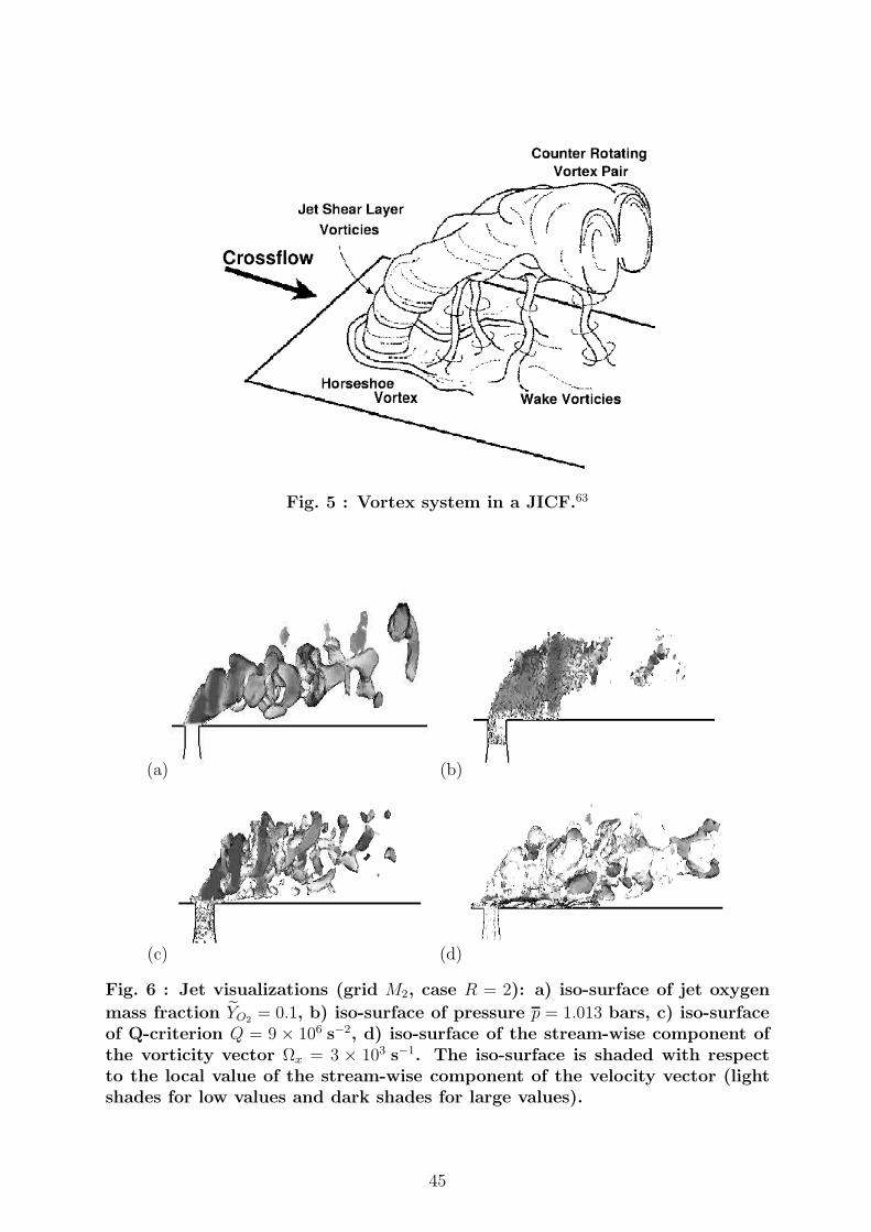
Fig. 5 : Vortex system in a JICF.63

(a) (b)

(c) (d)

Fig. 6 : Jet visualizations (grid M2, case R = 2): a) iso-surface of jet oxygen

mass fraction YO2= 0.1, b) iso-surface of pressure p = 1.013 bars, c) iso-surface

of Q-criterion Q = 9 × 106 s−2, d) iso-surface of the stream-wise component ofthe vorticity vector Ωx = 3 × 103 s−1. The iso-surface is shaded with respectto the local value of the stream-wise component of the velocity vector (lightshades for low values and dark shades for large values).

45

(a) (b)

(c) (d)

Fig. 7 : Jet visualizations (grid M2, case R = 4): a) iso-surface of jet oxygen

mass fraction YO2= 0.1, b) iso-surface of pressure p = 1.013 bars, c) iso-surface

of Q-criterion Q = 9 × 106 s−2, d) iso-surface of the stream-wise component ofthe vorticity vector Ωx = 3 × 103 s−1. All iso-surface is shaded with respectto the local value of the stream-wise component of the velocity vector (lightshades for low values and dark shades for large values).

(a) (b)

Fig. 8 : Levels of the normalized stream-wise vorticity Ωx , a) plane x = 1d, b)plane x = 2d.

46

(a)

(b)

Fig. 9 : Visualization of the CVP’s as obtained from (a) instantaneous and(b) mean fields. Each picture displays experimental views of PIV particletraces (top) and LES views of jet oxygen concentration (bottom). Dark grayrelates to large values of the concentrations and light gray corresponds to lowvalues. The cross-stream plane used for visualization is located (a) 1d and (b)5d downstream of the jet injection plane.

47

(a) (b)

Fig. 10 : Probe locations in the LES study of the wake region (dimensions arein millimeters): a) lateral view and b) top view.

(a)

0.0 0.2 0.4 0.6 0.8St

Vcf

0.0

0.5

1.0

1.5

2.0

2.5

3.0

Arb

itra

ry

sc

ale

LES results

LES smoothed results

(b)

Fig. 11 : Vortex shedding frequencies analysis in the wake region. a) LESpredictions, b) measurements.

48

Fig. 12 : Probe locations in the LES study of the jet shear layer region (di-mensions are in millimeters and shown for the plane z = 0).

(a)

0.0 0.1 0.2 0.3 0.4 0.5 0.6 0.7 0.8St

Vjet

0.0

0.2

0.4

0.6

0.8

Arb

itra

ry

sc

ale

LES results

LES smoothed results

(b)

Fig. 13 : Vortex shedding frequencies analysis in the jet shear layer region. a)LES predictions, b) measurements.

49

0.0 1.0 2.0

x=2d

0.0

0.1

0.2

0.3

0.4

0.5

r/D

1.0

x=5d

1.0

x=10d

Fig. 14 : Comparisons of the non-dimensionalized mean stream-wise compo-nent of the velocity vector, u/vcf , as obtained from the LES predictions andexperimental measurements (circles). Long dashed lines: grid M1 without TI,dotted lines: grid M2 without TI, and solid lines: grid M2 with TI.

50

(a)

(b)

(c)

Fig. 15 : Non-dimensionalized fields of the mean axial component of the veloc-ity vector, u/vcf , obtained with LES, left column and measured by ONERA,right column. The comparison is obtained for three downstream locations, a)x = 2d, b) x = 5d, c) x = 10d.

51

0.2 0.6

x=2d

0.0

0.1

0.2

0.3

0.4

0.5

r/D

0.2 0.4

x=5d0.2

x=10d

Fig. 16 : Comparisons of the non-dimensionalized fluctuation of the stream-wise velocity component, u′/vcf , as predicted by LES and obtained in theexperiment (circles). Long dashed lines: grid M1 without TI, dotted lines:grid M2 without TI, solid lines grid M2 with TI.

52

(a)

0 5 10 15

x/d

0

2

4

6

8

10

12

14

16

18

y/d

LES with TI, grid M2

LES without TI, grid M2

LES without TI, grid M1

ONERA

Patrick (1967)

Margason (1968)

Kamotani (1972)

Chassaing (1974)

Fearn (1978)

Hasselbrink (2004)

(b)

0 5 10 15

x/d

0

2

4

6

8

10

12

14

y/d

LES with TI, grid M2

LES without TI, grid M2

LES without TI, grid M1

ONERA

Patrick (1967)

Kamotani (1972)

Karagozian (1986)

Fig. 17 : Jet trajectories obtained by LES and the self-similar expressionsgiven in Table 3: a) maximum of the stream-wise component of velocity and,b) maximum of scalar concentration.

53

(a)

1 10

ln(s/Rd)

1

ln((

U−

vcf)/(

vje

t−v

cf))

LES with TI, grid M2

LES without TI, grid M2

LES without TI, grid M1

−1

−2/3

(b)

1 10

ln(s/Rd)

10

100

ln(Y

(%))

LES with TI, grid M2

LES without TI, grid M2

LES without TI, grid M1

−2/3

−1

Fig. 18 : Jet decay rates as predicted by LES: a), maximum stream-wisecomponent of the stream-wise component of velocity and b), maximum scalarconcentration. Solid lines represent the decay laws.

54

Tables

Table 1: Mesh characteristics.

GridTotal number

of nodesTotal number

of cellsFiner to largercell ratio (m)

M1 240, 000 1, 200, 000 3.5 × 10−4/8.2 × 10−3

M2 400, 000 2, 100, 000 3.5 × 10−4/5.2 × 10−3

Table 2: Boundary conditions.

Patch BC Imposed quantities Approach Relax Acoustic property

A Main inletu, v, w, T , Yα with

”turbulence injection”Thompson55 500 Partially reflective

B Jet inlets u, v, w, T , Yα Thompson55 500 Partially reflective

C Main outlet free-stream values Poinsot56 0.5 Partially reflective

D Main walls isothermal law of the wall Thompson55 - Reflective

E Jet walls isothermal no-slip walls Thompson55 - Reflective

55

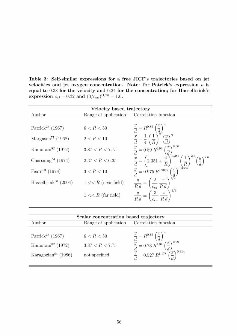
Table 3: Self-similar expressions for a free JICF’s trajectories based on jetvelocities and jet oxygen concentration. Note: for Patrick’s expression n isequal to 0.38 for the velocity and 0.34 for the concentration; for Hasselbrink’sexpression cej = 0.32 and (3/cew)(1/3) = 1.6.

Velocity based trajectoryAuthor Range of application Correlation function

Patrick78 (1967) 6 < R < 50y

d= R0.85

(x

d

)n

Margason77 (1968) 2 < R < 10x

d=

1

4

(1

R

)2 (y

d

)3

Kamotani82 (1972) 3.87 < R < 7.75y

d= 0.89 R0.94

(x

d

)0.36

Chassaing54 (1974) 2.37 < R < 6.35x

d=

(2.351 +

4

R

)0.385(1

R

)2.6(y

d

)2.6

Fearn83 (1978) 3 < R < 10y

d= 0.975 R0.9085

(x

d

)0.3385

Hasselbrink80 (2004) 1 << R (near field)y

R d=

(2

cej

x

R d

)1/2

1 << R (far field)y

R d=

(3

cew

x

R d

)1/3

Scalar concentration based trajectoryAuthor Range of application Correlation function

Patrick78 (1967) 6 < R < 50y

d= R0.85

(x

d

)n

Kamotani82 (1972) 3.87 < R < 7.75y

d= 0.73 R1.04

(x

d

)0.29

Karagozian84 (1986) not specifiedy

d= 0.527 R1.178

(x

d

)0.314

56