experimental and numerical analysis of heat transfer in a ... · experimental measurement of the...

EXPERIMENTAL AND NUMERICAL ANALYSIS OF HEAT

TRANSFER IN A PARTICLE-BASED CONCENTRATED

SOLAR POWER RECEIVER

by

Tyler C. Ketchem

A thesis submitted to the Faculty and the Board of Trustees of the Colorado School of

Mines in partial fulfillment of the requirements for the degree of Master of Science (Mechan-

ical Engineering).

Golden, Colorado

Date

Signed:Tyler C. Ketchem

Signed:Dr. Greg Jackson

Thesis Advisor

Signed:Dr. Robert Braun

Thesis Advisor

Golden, Colorado

Date

Signed:Dr. Greg Jackson

Professor and HeadDepartment of Mechanical Engineering

ii

ABSTRACT

A new concept has been developed by the National Renewable Energy Laboratory to

realize the advantages of particle-based concentrated solar power with thermal energy stor-

age. This concept uses an array of horizontal, hexagonal absorber tubes to capture sunlight

and transfer heat to particles flowing over the heated tube surfaces. The granular flow heat

transfer characteristics are critical to the design of the system but are not well understood.

This research seeks to characterize heat transfer within this solar receiver concept by exper-

imentally measuring heat transfer coefficients and developing a model capable of simulating

a full-scale receiver by utilizing existing heat transfer correlations.

Experiments conducted on a small-scale tube array showed the dynamic nature of the

particle flow and the dependence of the heat transfer coefficients on particle contact. The

top tube face has particle contact along its full length, the side face has intermittent contact

and the bottom face has little to none. The top face heat transfer coefficient was found to be

roughly 320 W/m2-K, over ten times greater than the bottom face, while the average heat

transfer coefficient for a single tube was roughly 175 W/m2-K using 300 µm particles.

A numerical model was then developed that includes both the solar and particle sides

of the absorber tubes. Three-dimensional view factor relations capture incoming flux and

reradiation effects while a unique heat transfer correlation from the literature was used for

each face. The top face was treated as an inclined plate, the side face as a smooth-walled

vertical channel, and the bottom face by considering heat transfer in a thin channel of the

pure gas phase. Relevant flow parameters for these correlations were obtained through a

one-dimensional model of the particle flow dynamics. Simulation of the full-scale receiver at

intended operating conditions shows significant improvement in the convective and effective

heat transfer coefficients due to increased bulk conductivity and thermal diffusivity of the

granular flow at high temperatures and greatly increased contributions from radiation.

iii

TABLE OF CONTENTS

ABSTRACT . . . . . . . . . . . . . . . . . . . . . . . . . . . . . . . . . . . . . . . . . iii

LIST OF FIGURES . . . . . . . . . . . . . . . . . . . . . . . . . . . . . . . . . . . . . vii

LIST OF TABLES . . . . . . . . . . . . . . . . . . . . . . . . . . . . . . . . . . . . . . . x

LIST OF SYMBOLS . . . . . . . . . . . . . . . . . . . . . . . . . . . . . . . . . . . . . xi

LIST OF ABBREVIATIONS . . . . . . . . . . . . . . . . . . . . . . . . . . . . . . . . xiv

ACKNOWLEDGMENTS . . . . . . . . . . . . . . . . . . . . . . . . . . . . . . . . . . xv

CHAPTER 1 INTRODUCTION . . . . . . . . . . . . . . . . . . . . . . . . . . . . . . . 1

1.1 Concentrated Solar Power Towers . . . . . . . . . . . . . . . . . . . . . . . . . . 1

1.2 Particle-Based CSP . . . . . . . . . . . . . . . . . . . . . . . . . . . . . . . . . . 2

1.3 Near-Blackbody Enclosed Particle Receiver Concept . . . . . . . . . . . . . . . . 3

1.4 Heat Transfer Considerations . . . . . . . . . . . . . . . . . . . . . . . . . . . . 4

1.5 Research Objectives . . . . . . . . . . . . . . . . . . . . . . . . . . . . . . . . . . 6

CHAPTER 2 LITERATURE REVIEW . . . . . . . . . . . . . . . . . . . . . . . . . . . 7

2.1 Heat Transfer in Granular Flows . . . . . . . . . . . . . . . . . . . . . . . . . . . 7

2.1.1 Fluidized Beds . . . . . . . . . . . . . . . . . . . . . . . . . . . . . . . . 7

2.1.2 Tube Bundles . . . . . . . . . . . . . . . . . . . . . . . . . . . . . . . . . 8

2.1.3 Flat Plates . . . . . . . . . . . . . . . . . . . . . . . . . . . . . . . . . . 9

2.1.4 Vertical Channels . . . . . . . . . . . . . . . . . . . . . . . . . . . . . . 10

2.1.5 Pneumatic Transport of Particles . . . . . . . . . . . . . . . . . . . . . 10

2.2 Granular Flow Dynamics . . . . . . . . . . . . . . . . . . . . . . . . . . . . . . 10

iv

CHAPTER 3 EXPERIMENTS . . . . . . . . . . . . . . . . . . . . . . . . . . . . . . . 12

3.1 Objective . . . . . . . . . . . . . . . . . . . . . . . . . . . . . . . . . . . . . . 12

3.2 Test Setup . . . . . . . . . . . . . . . . . . . . . . . . . . . . . . . . . . . . . . 12

3.2.1 Electrical Control System and Data Acquisition . . . . . . . . . . . . . 16

3.2.2 Material Properties . . . . . . . . . . . . . . . . . . . . . . . . . . . . . 17

3.3 Heat Transfer Testing Procedure . . . . . . . . . . . . . . . . . . . . . . . . . . 19

3.3.1 Average Heat Transfer Data Analysis . . . . . . . . . . . . . . . . . . . 19

3.3.2 “Local” Heat Transfer Coefficient Analysis . . . . . . . . . . . . . . . . 21

3.4 Results . . . . . . . . . . . . . . . . . . . . . . . . . . . . . . . . . . . . . . . . 23

3.4.1 Flow Visualization . . . . . . . . . . . . . . . . . . . . . . . . . . . . . 25

3.5 Results Discussion . . . . . . . . . . . . . . . . . . . . . . . . . . . . . . . . . 26

CHAPTER 4 MODELING APPROACH . . . . . . . . . . . . . . . . . . . . . . . . . 27

4.1 Modeling Methodology . . . . . . . . . . . . . . . . . . . . . . . . . . . . . . . 27

4.2 Tube Wall Equations . . . . . . . . . . . . . . . . . . . . . . . . . . . . . . . . 29

4.2.1 Tube Wall Conductivity . . . . . . . . . . . . . . . . . . . . . . . . . . 30

4.2.2 Radiation View Factors . . . . . . . . . . . . . . . . . . . . . . . . . . . 31

4.3 Heat Transfer Correlations . . . . . . . . . . . . . . . . . . . . . . . . . . . . . 34

4.3.1 Top Face . . . . . . . . . . . . . . . . . . . . . . . . . . . . . . . . . . . 35

4.3.2 Side Face . . . . . . . . . . . . . . . . . . . . . . . . . . . . . . . . . . 35

4.3.3 Bottom Face . . . . . . . . . . . . . . . . . . . . . . . . . . . . . . . . . 36

4.3.4 Effective Heat Transfer Coefficient . . . . . . . . . . . . . . . . . . . . . 38

4.3.5 Particle Phase Conductivity . . . . . . . . . . . . . . . . . . . . . . . . 39

4.4 1D Granular Flow Modeling . . . . . . . . . . . . . . . . . . . . . . . . . . . . 39

v

4.4.1 Solid Phase Continuity . . . . . . . . . . . . . . . . . . . . . . . . . . . 40

4.4.2 Solid Phase Momentum . . . . . . . . . . . . . . . . . . . . . . . . . . 41

4.4.3 Gas Phase Continuity . . . . . . . . . . . . . . . . . . . . . . . . . . . 42

4.4.4 Solid Phase Energy . . . . . . . . . . . . . . . . . . . . . . . . . . . . . 42

4.4.5 Inlet Conditions . . . . . . . . . . . . . . . . . . . . . . . . . . . . . . . 43

4.5 Input Parameter Selection Based on Comparison to Experimental Data . . . . 43

4.5.1 Particle Flow Depth Considerations . . . . . . . . . . . . . . . . . . . . 43

4.5.2 Heat Transfer Considerations . . . . . . . . . . . . . . . . . . . . . . . 45

4.5.3 Parameter Selection . . . . . . . . . . . . . . . . . . . . . . . . . . . . . 47

4.6 Model Validation . . . . . . . . . . . . . . . . . . . . . . . . . . . . . . . . . . 49

4.7 Numerical Parameters . . . . . . . . . . . . . . . . . . . . . . . . . . . . . . . 51

4.8 Discussion . . . . . . . . . . . . . . . . . . . . . . . . . . . . . . . . . . . . . . 52

CHAPTER 5 RECEIVER ANALYSIS . . . . . . . . . . . . . . . . . . . . . . . . . . . 54

5.1 Heat Transfer Correlation Analysis . . . . . . . . . . . . . . . . . . . . . . . . 54

5.2 Full Receiver Simulations . . . . . . . . . . . . . . . . . . . . . . . . . . . . . . 56

5.2.1 Particle Flow Results . . . . . . . . . . . . . . . . . . . . . . . . . . . . 57

5.2.2 Heat Transfer Results . . . . . . . . . . . . . . . . . . . . . . . . . . . 57

5.3 Full Receiver Simulation Discussion . . . . . . . . . . . . . . . . . . . . . . . . 61

CHAPTER 6 SUMMARY & CONCLUSIONS . . . . . . . . . . . . . . . . . . . . . . 63

6.1 Future Work . . . . . . . . . . . . . . . . . . . . . . . . . . . . . . . . . . . . . 65

REFERENCES CITED . . . . . . . . . . . . . . . . . . . . . . . . . . . . . . . . . . . 67

vi

LIST OF FIGURES

Figure 1.1 Near-Blackbody particle receiver design diagram . . . . . . . . . . . . . . . 4

Figure 3.1 Test stand used for experiments . . . . . . . . . . . . . . . . . . . . . . . 13

Figure 3.2 Instrumented tube setup used for experiments . . . . . . . . . . . . . . . 14

Figure 3.3 Single heated tube cross-sectional diagram . . . . . . . . . . . . . . . . . 15

Figure 3.4 Dimensions of heated tubes used in experiments . . . . . . . . . . . . . . 15

Figure 3.5 Instrumented tube for “local” heat transfer measurements . . . . . . . . . 16

Figure 3.6 Custom-built test stand electronics . . . . . . . . . . . . . . . . . . . . . 17

Figure 3.7 Particle batch sieve curves . . . . . . . . . . . . . . . . . . . . . . . . . . 18

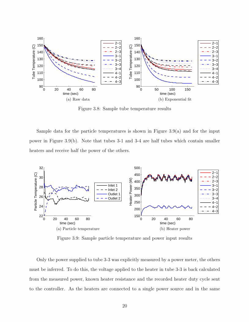
Figure 3.8 Sample tube temperature results . . . . . . . . . . . . . . . . . . . . . . . 20

Figure 3.9 Sample particle temperature and power input results . . . . . . . . . . . . 20

Figure 3.10 Fluent setup and boundary conditions for “local” heat transfercoefficients . . . . . . . . . . . . . . . . . . . . . . . . . . . . . . . . . . . 22

Figure 3.11 A sample of Fluent temperature results along the side of a single tubefrom top to bottom vertexes compared to experimental data . . . . . . . 23

Figure 3.12 Average heat transfer coefficient results . . . . . . . . . . . . . . . . . . . 24

Figure 3.13 Local heat transfer coefficient results by face for the 300 µm particlebatch . . . . . . . . . . . . . . . . . . . . . . . . . . . . . . . . . . . . . . 24

Figure 3.14 Local heat transfer coefficient results by face for the 200 µm particlebatch . . . . . . . . . . . . . . . . . . . . . . . . . . . . . . . . . . . . . . 24

Figure 3.15 Particle flow visualization results . . . . . . . . . . . . . . . . . . . . . . . 25

Figure 4.1 Discretized domain used for modeling . . . . . . . . . . . . . . . . . . . . 28

Figure 4.2 MATLAB program flow chart . . . . . . . . . . . . . . . . . . . . . . . . 28

vii

Figure 4.3 Control volume used for tube wall nodes with energy flows . . . . . . . . 29

Figure 4.4 Tube input dimensions . . . . . . . . . . . . . . . . . . . . . . . . . . . . 31

Figure 4.5 Offset parallel planes configuration . . . . . . . . . . . . . . . . . . . . . . 32

Figure 4.6 Contacting planes view factor diagram . . . . . . . . . . . . . . . . . . . 33

Figure 4.7 Adjacent planes diagram . . . . . . . . . . . . . . . . . . . . . . . . . . . 34

Figure 4.8 Development of Nusselt number fit curve . . . . . . . . . . . . . . . . . . 37

Figure 4.9 Control volume for particle flow nodes with relevant variables andparameters . . . . . . . . . . . . . . . . . . . . . . . . . . . . . . . . . . . 40

Figure 4.10 Sample results . . . . . . . . . . . . . . . . . . . . . . . . . . . . . . . . . 44

Figure 4.11 Flow depth considerations at maximum flow conditions . . . . . . . . . . 45

Figure 4.12 Side face heat transfer analysis vs the relevant parameters . . . . . . . . . 46

Figure 4.13 Bottom face heat transfer analysis vs the relevant parameters . . . . . . . 46

Figure 4.14 Top face heat transfer analysis vs the relevant parameters . . . . . . . . . 47

Figure 4.15 All considerations for parameter selection . . . . . . . . . . . . . . . . . . 48

Figure 4.16 Flow depth considerations . . . . . . . . . . . . . . . . . . . . . . . . . . 49

Figure 4.17 300 micron simulation vs 300 µm particle batch data . . . . . . . . . . . . 50



Figure 4.20 Numerical Parameters Comparison . . . . . . . . . . . . . . . . . . . . . . 52

Figure 5.1 Direct heat transfer correlation analysis results . . . . . . . . . . . . . . . 55

Figure 5.2 Fully developed particle flow dynamics results . . . . . . . . . . . . . . . 57

Figure 5.3 Average flow conditions . . . . . . . . . . . . . . . . . . . . . . . . . . . . 58

Figure 5.4 Temperature results . . . . . . . . . . . . . . . . . . . . . . . . . . . . . . 58

viii

Figure 5.5 Average heat transfer coefficients per face by row . . . . . . . . . . . . . . 59

Figure 5.6 Normalized tube energy balances for each tube node . . . . . . . . . . . . 60

ix

LIST OF TABLES

Table 3.1 Specifications of thermocouples used in experiments . . . . . . . . . . . . . 16

Table 3.2 Composition of particles used in experiments . . . . . . . . . . . . . . . . . 18

Table 3.3 Properties of particles used in experiments . . . . . . . . . . . . . . . . . . 18

Table 4.1 Input parameters for comparison to experimental data . . . . . . . . . . . . 44

Table 4.2 Acceptable parameter inputs based on comparison to experimental data . . 48

Table 5.1 Input parameters used for full NBB receiver simulation . . . . . . . . . . . 56

Table 6.1 Experimentally determined average heat transfer coefficients for each faceat maximum particle flow conditions using 300 µm particles at 25°C . . . . 63

Table 6.2 Model predicted average heat transfer coefficients for each face atmaximum particle flow conditions using 300 µm particles at 800°C . . . . . 65

x

LIST OF SYMBOLS

Modified Froude number . . . . . . . . . . . . . . . . . . . . . . . . . . . . . . . . . . Fr∗

Average Nusselt number defined by hydraulic diameter . . . . . . . . . . . . . . . . . NuD

Average Nusselt number defined by particle diameter . . . . . . . . . . . . . . . . . . Nu∗d

Local Nusselt number . . . . . . . . . . . . . . . . . . . . . . . . . . . . . . . . . . . Nux

Modified Peclet number . . . . . . . . . . . . . . . . . . . . . . . . . . . . . . . . . . Pe∗L

Prandtl number . . . . . . . . . . . . . . . . . . . . . . . . . . . . . . . . . . . . . . . . Pr

Reynolds number . . . . . . . . . . . . . . . . . . . . . . . . . . . . . . . . . . . . . . . Re

Tube surface area . . . . . . . . . . . . . . . . . . . . . . . . . . . . . . . . . . . . . . . At

Particle phase specific heat . . . . . . . . . . . . . . . . . . . . . . . . . . . . . . . . . cp

Particle flow depth . . . . . . . . . . . . . . . . . . . . . . . . . . . . . . . . . . . . . . . d

Hydraulic diameter . . . . . . . . . . . . . . . . . . . . . . . . . . . . . . . . . . . . . . Dh

Length of node in particle flow direction . . . . . . . . . . . . . . . . . . . . . . . . . . dx

Average particle diameter . . . . . . . . . . . . . . . . . . . . . . . . . . . . . . . . . . dp

Inner tube surface emissivity . . . . . . . . . . . . . . . . . . . . . . . . . . . . . . . . ein

Particle material emissivity . . . . . . . . . . . . . . . . . . . . . . . . . . . . . . . . . ep

Particle curtain emissivity . . . . . . . . . . . . . . . . . . . . . . . . . . . . . . . . . . ec

Tube particle side emissivity . . . . . . . . . . . . . . . . . . . . . . . . . . . . . . . . . et

Radiation view factor . . . . . . . . . . . . . . . . . . . . . . . . . . . . . . . . . . . . Fi,j

Gravitationl constant . . . . . . . . . . . . . . . . . . . . . . . . . . . . . . . . . . . . . . g

Channel height . . . . . . . . . . . . . . . . . . . . . . . . . . . . . . . . . . . . . . . . H

xi

Average convective heat transfer coefficient . . . . . . . . . . . . . . . . . . . . . . . . . h

Convective heat transfer coefficient . . . . . . . . . . . . . . . . . . . . . . . . . . . . hconv

Effective heat transfer coefficient . . . . . . . . . . . . . . . . . . . . . . . . . . . . . heff

Bulk conductivity of particle phase . . . . . . . . . . . . . . . . . . . . . . . . . . . . . . k

Gas phase conductivity . . . . . . . . . . . . . . . . . . . . . . . . . . . . . . . . . . . . kg

Solids material conductivity . . . . . . . . . . . . . . . . . . . . . . . . . . . . . . . . . ks

Tube wall conductivity . . . . . . . . . . . . . . . . . . . . . . . . . . . . . . . . . . . . kt

Plate length . . . . . . . . . . . . . . . . . . . . . . . . . . . . . . . . . . . . . . . . . . L

Tube length . . . . . . . . . . . . . . . . . . . . . . . . . . . . . . . . . . . . . . . . . . Lt

Particle mass flow rate . . . . . . . . . . . . . . . . . . . . . . . . . . . . . . . . . . . . m

Nodes per tube face . . . . . . . . . . . . . . . . . . . . . . . . . . . . . . . . . . . . Nface

Volumetric energy input . . . . . . . . . . . . . . . . . . . . . . . . . . . . . . . . . . . . q

Heater power . . . . . . . . . . . . . . . . . . . . . . . . . . . . . . . . . . . . . . . . . qh

Incoming solar flux . . . . . . . . . . . . . . . . . . . . . . . . . . . . . . . . . . . . . q′′solar

Cold reservoir temperature . . . . . . . . . . . . . . . . . . . . . . . . . . . . . . . . . . TC

Gas temperature . . . . . . . . . . . . . . . . . . . . . . . . . . . . . . . . . . . . . . . Tg

Mean gas temperature . . . . . . . . . . . . . . . . . . . . . . . . . . . . . . . . . . . . Tg

Hot reservoir temperature . . . . . . . . . . . . . . . . . . . . . . . . . . . . . . . . . . TH

Tube wall temprature . . . . . . . . . . . . . . . . . . . . . . . . . . . . . . . . . . . . Tt

Particle temperature . . . . . . . . . . . . . . . . . . . . . . . . . . . . . . . . . . . . . Tp

Wall temperature adjacent to particle flow . . . . . . . . . . . . . . . . . . . . . . . . TW

Air channel height/thickness . . . . . . . . . . . . . . . . . . . . . . . . . . . . . . . . . . t

Tube wall thickness . . . . . . . . . . . . . . . . . . . . . . . . . . . . . . . . . . . . . . tt

xii

Average particle flow velocity . . . . . . . . . . . . . . . . . . . . . . . . . . . . . . . . . v

Average gas velocitty . . . . . . . . . . . . . . . . . . . . . . . . . . . . . . . . . . . . . vg

Channel width . . . . . . . . . . . . . . . . . . . . . . . . . . . . . . . . . . . . . . . . W

“Effective” film thickness . . . . . . . . . . . . . . . . . . . . . . . . . . . . . . . . . xeff

Dimensionless entry length . . . . . . . . . . . . . . . . . . . . . . . . . . . . . . . . . . x∗

Particle curtain thickness . . . . . . . . . . . . . . . . . . . . . . . . . . . . . . . . . . zc

Particle phase thermal diffusivity . . . . . . . . . . . . . . . . . . . . . . . . . . . α = kρcp

Heat transfer empirical constant . . . . . . . . . . . . . . . . . . . . . . . . . . . . . . . β

Ergun particle drag coefficient . . . . . . . . . . . . . . . . . . . . . . . . . . . . . . . . βv

Gas volume fraction within the particle flow . . . . . . . . . . . . . . . . . . . . . . . . γ

Bed friction coefficient . . . . . . . . . . . . . . . . . . . . . . . . . . . . . . . . . . . . . δ

Temperature residual criteria . . . . . . . . . . . . . . . . . . . . . . . . . . . . . . ∆Tres

Solids volume fraction within flow depth . . . . . . . . . . . . . . . . . . . . . . . . . . . ε

Critical solids volume fraction . . . . . . . . . . . . . . . . . . . . . . . . . . . . . . . . εc

Carnot efficiency . . . . . . . . . . . . . . . . . . . . . . . . . . . . . . . . . . . . . ηCarnot

Plate inclination angle . . . . . . . . . . . . . . . . . . . . . . . . . . . . . . . . . . . . . θ

Gas viscosity . . . . . . . . . . . . . . . . . . . . . . . . . . . . . . . . . . . . . . . . . µg

Bulk particle phase density . . . . . . . . . . . . . . . . . . . . . . . . . . . . . . ρ = ερs

Gas density . . . . . . . . . . . . . . . . . . . . . . . . . . . . . . . . . . . . . . . . . . ρg

Solids material density . . . . . . . . . . . . . . . . . . . . . . . . . . . . . . . . . . . . ρs

Stephen-Boltzmann constant . . . . . . . . . . . . . . . . . . . . . . . . . . . . . . . . σ

Particle curtain transmissivity . . . . . . . . . . . . . . . . . . . . . . . . . . . . . . . . τc

xiii

LIST OF ABBREVIATIONS

Photovoltaic . . . . . . . . . . . . . . . . . . . . . . . . . . . . . . . . . . . . . . . . . PV

Concentrated Solar Power . . . . . . . . . . . . . . . . . . . . . . . . . . . . . . . . . CSP

Thermal Energy Storage . . . . . . . . . . . . . . . . . . . . . . . . . . . . . . . . . . TES

National Renewable Energy Laboratory . . . . . . . . . . . . . . . . . . . . . . . . NREL

Near-Blackbody . . . . . . . . . . . . . . . . . . . . . . . . . . . . . . . . . . . . . . NBB

User-Defined Function . . . . . . . . . . . . . . . . . . . . . . . . . . . . . . . . . . UDF

Heat Transfer Coefficient . . . . . . . . . . . . . . . . . . . . . . . . . . . . . . . . . HTC

xiv

ACKNOWLEDGMENTS

I would foremost like to thank my advisors, Dr. Greg Jackson and Dr. Robert Braun,

for their assistance on this project. I would also like to thank Dr. Zhiwen Ma for allow-

ing me to include the details of his Near-Blackbody solar receiver concept and Dr. Janna

Martinek for her assistance in developing models for data analysis and advice in modeling.

Additionally, I would like to thank the rest of the Concentrated Solar Power research group

at the National Renewable Energy Laboratory for their assistance with the granular flow

heat transfer experiments with a special thanks to Dr. Greg Glatzmaier for his efforts on

the heater control system. Lastly, I would like to thank my fellow graduate students for all

of their help and support.

xv

CHAPTER 1

INTRODUCTION

Each day, more energy reaches the earth from the sun than is used by mankind in an

entire year [1]. Harvesting even a small fraction of this energy has the potential to meet

a large portion of the world’s growing energy demand with clean renewable energy. This

abundant solar energy can be captured through both photovoltaics (PV) and concentrated

solar power (CSP) technologies. Although PV panels can be installed almost anywhere and

are ever increasing in efficiency, CSP utilizing a central receiver tower holds great promise

to deliver cost-effective, dispatchable utility-scale electricity [2]. This is in large part due to

its ability to generate power on the MW scale while incorporating thermal energy storage

(TES).

1.1 Concentrated Solar Power Towers

Concentrated solar power systems operate by using mirrors, or heliostats, to focus the

sun’s energy onto a central location to warm a heat transfer fluid. The hot fluid can then be

sent through a power cycle to produce electricity or transfer its energy to a separate working

fluid that runs a power cycle. In the case of a single fluid system, water is typically used as

the heat transfer fluid and converted directly to steam within the solar receiver. Ongoing

research seeks to directly heat gases, such as CO2, to power high temperature Brayton

cycles [3]. For two-fluid systems, oils are used as the heat transfer fluid and steam as the

working fluid. These configurations only allow for power production during periods of high

solar irradiance and can have significant intermittency. Incorporating TES can overcome

this intermittency problem and add value to the plant by allowing for load following and

overnight electricity production [4].

Thermal energy can be stored as purely sensible heat, latent heat or as thermochemical

energy and can be achieved in two configurations, direct or indirect. In an indirect system,

1

the energy of the heat transfer fluid is transferred to an energy storage medium. Alternatives

considered for use as the storage medium include liquids, solid slabs of concrete and packed

beds of inert solids, thermochemically reacting solids or phase change materials [5–7]. Al-

ternatively, a direct system utilizes the heat transfer fluid as the thermal storage medium.

In both configurations, energy from the storage medium is transferred to a working fluid to

run a power cycle when desired.

Current state of the art TES systems use molten nitrate salts as both the heat transfer

fluid and thermal storage medium in a direct configuration as shown in [5]. The salts are

pumped through the receiver between hot and cold storage tanks. Electricity is generated

by transferring energy from the salts to create steam and power a Rankine cycle. The

use of these exotic materials, as well as the equipment needed to move these fluids, create

significant costs. Additionally, the operating temperatures of these plants are limited by

the temperature limitations of the salts [8]. Freezing issues are encountered at 220°C and

corrosion and chemical break down occur above 650°C [9]. These temperature constraints

present a significant barrier to performance. As CSP plants operate using thermodynamic

power cycles, their efficiency is governed by thermodynamic principles and limited by the

Carnot efficiency:

ηCarnot = 1− TC

TH

(1.1)

where TH is the temperature of the hot reservoir and TC is the temperature of the cold

reservoir, which is the ambient air temperature in this case. Increased efficiency, and therefore

improved cost, can be achieved by increasing the upper temperature limits. Unfortunately,

as discussed, current systems already operate at the upper limits of molten salts. A change

in heat transfer fluids is therefore needed.

1.2 Particle-Based CSP

In the 1980’s it was proposed that solid particles could be utilized as the heat transfer

medium in CSP plants [10–13]. Utilizing solid particles offers several advantages over nitrate

2

salts for CSP systems. The primary benefit is the potential for higher operating tempera-

tures. When particles such as sand are utilized, heat transfer fluid temperatures can feasibly

exceed 1000°C, greatly boosting power cycle efficiency [12, 14]. Operating temperatures are

instead limited by the temperature limitations of structural components and efficiency is

limited by the increasing reradiation losses from high temperature surfaces.

Like molten salts, particles can serve as both the thermal storage medium and the heat

transfer fluid in a direct configuration. While stored in a packed bed silo, the granular nature

of solid particles offers the unique advantage of self-insulation [9]. A temperature gradient

forms across a layer of particles near the wall that acts as insulation and limits further heat

loss. Energy can still be effectively transferred from the hot particles to a working fluid

through the use of a fluidized bed. Additionally, the use of solid particles, such as sand,

offers significant cost benefits as they are low-cost materials in comparison to molten salts.

The primary design challenge in particle-based systems is the heating of the particles

as they cannot simply be pumped through irradiated tubing like a liquid. Many design

configurations have been proposed [15, 16], with the most widely studied option being the

falling curtain receiver [14, 17]. This design directly irradiates the particles by dropping

them in a steady stream through the path of concentrated sunlight. A significant drawback

of this configuration is the low residence time of the particles in the irradiated zone caused

by high velocities during free fall. This leads to low particle outlet temperatures. As the

particles fall, considerable thinning of the particle curtain also occurs which leads to a large

portion of the sun’s energy directly heating the back wall of the enclosure instead of the

particles. The high temperature of the wall can lead to significant reradiation losses and

structural damage [14].

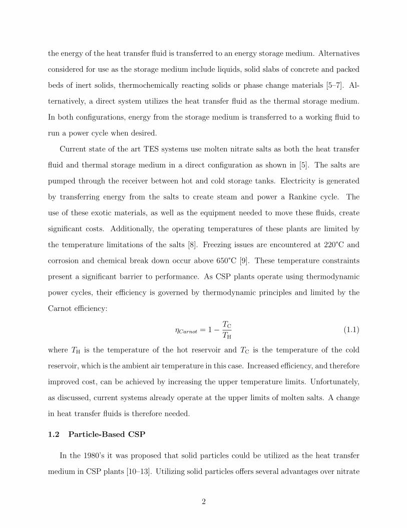
1.3 Near-Blackbody Enclosed Particle Receiver Concept

A new concept developed by the National Renewable Energy Laboratory (NREL) seeks

to overcome the shortcomings of existing particle-based receiver designs. This design, as

shown in Figure 1.1, utilizes an array of hollow, hexagonal tubes to capture the solar energy

3

directed by the heliostat field [18, 19]. Sunlight enters the tubes where it is spread along

the length of the tube by internal reflection and reradiation. This shape seeks to emulate a

blackbody by focusing the majority of reradiation from the tube walls onto adjacent tube

walls. Reradiation losses to the environment are therefore greatly reduced. Particles are

heated by contact with the hot tube surfaces as they cascade through the channels between

the backsides of the absorber tubes. A flair on the front of each tube connects the tubes

together while maintaining space between them for particle flow. A full-sized receiver will

consist of hundreds of rows of absorber tubes designed for particle outlet temperatures of

800°C or higher.

Solar Flux

Particle Flow

Figure 1.1: Near-Blackbody particle receiver design diagram (figure in part from [18])

1.4 Heat Transfer Considerations

An important component of the design of the NBB system is the heat transfer between the

absorber tubes and the particle flow. This heat transfer largely determines the temperature

of the absorber tubes for a given solar flux condition. Maximum tube temperatures drive

material selection, which significantly impacts cost. Excessive temperatures could exceed

the thermal limits of even the highest rated materials. Additionally, high tube temperatures

lead to increased reradiation losses and decrease overall system performance. It is therefore

4

imperative to thoroughly understand the heat transfer characteristics within the granular

flow to properly design the system.

Unfortunately, heat transfer in a cascading granular flow, such as this, is complex and

not well understood. A considerable number of granular flow heat transfer studies have been

performed in the literature [20–35], but no correlations exist that can directly predict heat

transfer in this configuration with reasonable confidence. A great deal of modeling has also

been undertaken to study heat transfer in particle-based CSP systems [13, 14, 16, 18]. This

literature largely focuses on falling curtain receivers that exhibit very different flow conditions

than those seen in the NBB design. These models use a variety of solar radiation models

and typically utilize full Lagrangian particle tracking in conjunction with fluid dynamics

modeling.

Efforts by NREL to model the cascading flow seen in the NBB design have provided

limited insight due to the challenges of the complex, multiphase heat transfer under consid-

eration [18]. The model developed focuses on a single tube within the receiver array and

utilizes the two-fluid model available in ANSYS Fluent. Results show heat transfer coeffi-

cients for the upper tube surface exceeding 1000 W/m2-K and almost negligibly small for

the side and bottom surfaces. The average heat transfer coefficient predicted for a single

tube, therefore, is considerably lower than those observed in previous small-scale experiments

[18]. This is in large part due to the perfect symmetry observed in the Fluent results that

does not match the more chaotic patterns and increased particle-wall contact observed in

the experiments. More complex models incorporating Lagrangian particle tracking, such as

those used for falling curtain designs, could prove more effective, but are too computationally

intensive for a full NBB system simulation and are not typically applicable for flows with

volume fractions exceeding 10% [14, 18]. It is therefore necessary to find alternative ways to

model the system and to directly measure the heat transfer coefficients more thoroughly for

a more comprehensive comparison.

5

1.5 Research Objectives

This research seeks to characterize and simulate heat transfer between the heated ab-

sorber tubes and the cascading granular flow to support and inform effective NBB receiver

design. This heat transfer is greatly impacted by the nature of the granular flow and is not

well understood. Specifically, this research aims to:

• Experimentally determine an average heat transfer coefficient for each face of the hexag-

onal absorber tubes

• Develop a numerical model for heat transfer within the NBB design capable of pre-

dicting the experimental results by utilizing existing literature correlations

• Use the model to predict heat transfer coefficients outside the range of experiments

and simulate a full-sized NBB solar receiver at intended operating conditions

These objectives are addressed by first examining the relevant literature in Chapter 2.

Experimental measurement of the heat transfer coefficient is discussed in Chapter 3. Chapter

4 outlines the approach and equations used in modeling the NBB receiver design and includes

a comparison to the experimental results. Simulation of a full-sized NBB receiver is discussed

in Chapter 5 with overall conclusions given in Chapter 6.

6

CHAPTER 2

LITERATURE REVIEW

In order to fully characterize heat transfer within the NBB design it is important to

understand the effects of all heat transfer modes. The dense granular flows within the design

have well known radiation effects, therefore, it is important to focus on understanding heat

transfer through convection and by direct particle contact. It is also important to understand

the granular flow dynamics and their impact on heat transfer. Although no previous studies

focused on granular flow in a configuration exactly like the NBB design, there is an abundance

of existing literature that can be utilized in its analysis. These include other CSP modeling

efforts as well as studies examining the heat transfer and flow characteristics of granular

flows in a variety of other configurations.

2.1 Heat Transfer in Granular Flows

The relevant literature pertaining to heat transfer in granular flows can be divided into

fluidized beds [20–24], flows over tube bundles [25–27], flows over flat plates [28–31], flows

in vertical channels [28, 32, 33] and pneumatic conveying of particles [34, 35].

2.1.1 Fluidized Beds

The work pertaining to fluidized beds is largely summarized in the work of Chen [20].

Chen argues that the many empirical correlations developed through numerical fitting of

experimental data [21–23] have limited use as their applicability only covers the narrow

range of operating conditions used in their development. Instead, the use of a mechanistic

model is advocated. The most widely accepted model stems from the work of Mickley and

Fairbanks [24]. This model is developed by considering discrete packets of particles that

move as a unit and persist for short time intervals. These packets circulate through the bed

and periodically contact the heat transfer surfaces and transfer heat. An important finding

7

from this work is the dependence of the heat transfer coefficient upon the square root of

the conductivity of the particle phase. Chen refers to this as the surface renewal model and

developed an equation to solve directly for the heat transfer coefficient in fluidized beds that

better encompasses the trends found in multiple experimental settings.

2.1.2 Tube Bundles

Studies considering heat transfer between horizontal tube bundles and granular material

focus on circular tubes and include fluidized bed [23] (discussed above), plug flow [25–27]

and trickling flow [36] applications. In plug flow the particles move more slowly than in free

fall conditions and are found to maintain contact with the tubes except for a small section of

flow separation at the bottom of each tube. Particles also collect on the upper tube surface

and form a pyramid shaped wedge of stagnant particles. The exact shape and size of the

stagnation zone depends upon the arrangement of the tubes and not the flow velocity [25].

Heat transfer is found to be minimal in the stagnation zone above the tube as well as in the

void zone below the tube and instead primarily occurs along the sides of the tube. Increasing

the mass flow rate improves overall heat transfer [26].

For trickling granular flow over a staggered bank of horizontal tubes, the particles are

again seen to collect and form a stagnation zone on the upper surface. The entire bottom half

of the tube has virtually no contact due to separation from the surface in free fall conditions.

The heat transfer coefficient for the upper surface is, therefore, much greater than for the

lower surface. The peak heat transfer coefficient occurs at the stagnation point for low mass

flow rates but moves along the perimeter towards a point at an angle of 45° from the vertical

as mass flow rates increase. This is due to increased accumulation of particles with increasing

mass flow rates that inhibit heat transfer at the stagnation point. Increasing the mass flow

rate leads to an overall increase in heat transfer, however. It was also found that decreasing

both the tube diameter and the particle size improve heat transfer [36].

8

2.1.3 Flat Plates

A simple configuration that has been relatively widely studied is that of the flat plate.

There are two fundamental ways to examine such a granular flow. The first is by considering

it to be a collection of discrete particles and the second is to assume a continuum, more similar

to a conventional fluid. By developing equations governing each situation and comparing

these to experimental data, Sullivan and Sabersky [28] found that a combination of these

approaches is most appropriate. Their preferred model treats granular flow as a continuum

with a thermal resistance at the contact surface. This is because the granular nature of

the particles allows for adequate particle to particle contact but results in poor contact at

the heat transfer surface. Thermal resistance is modeled as pure conduction through a thin

layer of the interstitial gas phase. The thickness of this layer is referred to as the ”effective”

film thickness. Experimental results of plug flow down a heated, vertical chute showed an

“effective” film thickness of 1/10 the diameter of a single particle. The resulting correlation

is dependent upon the “effective” film thickness as well as a modified Peclet number.

This concept was expanded to inclined channels and analyzed over a wider range of

Peclet numbers by the work of Spelt, Brennan and Sabersky [29]. It was discovered that

the heat transfer coefficient increased with increasing velocity, as expected, but only to a

certain point, after which the heat transfer decreased with continued increases in velocity.

The values at high Peclet numbers therefore deviated from those predicted by the Sullivan

and Sabersky correlation. This was believed to be due to changes in the density near the

heated surface. It was also discovered that the heat transfer coefficient was dependent upon

the depth of the flow, a parameter not previously encountered. The work of Patton et al

[30] developed an updated heat transfer correlation to capture these effects by measuring the

bulk flow density for each test. This led to the inclusion of a modified Froude number and

a correlation for heat transfer dependent upon the inclination angle and flow depth. The

applicability of this heat transfer correlation was validated through experiments by Golob

[31].

9

2.1.4 Vertical Channels

Granular flow through a vertical channel was considered by Sullivan and Sabersky in

developing the “effective” film thickness concept [28]. The experiments considered plug flow

through a vertical channel with smooth walls. This work was further expanded by the work

of Natarajan and Hunt [32, 33]. They showed that heat transfer in sheared flows in vertical

channels, simulated by using rough walls, did not follow the equation developed by Sullivan

and Sabersky beyond low Peclet numbers. Heat transfer in these cases was considerably

lower and showed a peak Nusselt number at a critical Peclet number before decreasing. This

decrease is not seen in plug flows. A model based on the kinetic theory of gases was developed

that more accurately predicts heat transfer for shear flows. A simple correlation like those

for flat plates was not developed.

2.1.5 Pneumatic Transport of Particles

An additional case studied is that of heat transfer during pneumatic conveying of particles

[34, 35]. This is a case often encountered in industrial applications. Studies focus on low

particle volume fractions and mostly depend upon convection through the flowing gas. It

was also determined that increases in particle volume fractions improve heat transfer up to

a certain point before a critical value is reached. Further addition of particles impedes their

ability to adequately mix and decreases heat transfer.

2.2 Granular Flow Dynamics

While the Navier-Stokes equations can be used to describe fluid flow, there are currently

no constitutive equations capable of completely describing granular flow [37]. Granular

flows are instead characterized by three different regimes. These are a “dense quasi-static”

regime, a “gaseous” regime and a “liquid” regime between the two [37]. The liquid regime

is most similar to the dense granular flow under consideration. In such a flow, the particles

largely maintain contact with one another and both collision and friction interactions play

a significant roll. Such flows are widely studied in a variety of configurations as discussed in

10

both [37] and [38]. The primary configuration applicable to this research is the flat plate.

Granular flows down flat plates can be divided into dilute or dense flows over either flat,

frictional bases or “bumpy” bases [39]. For dense flows over flat bases, a shear layer develops

near the surface which supports a plug flow above. Nearly constant volume fractions and

velocities are observed through the depth of the flow [39, 40]. Additionally, the volume

fraction is observed to be constant along the length of the plate. This constant value is

dependent upon the inclination angle and decreases for steeper inclines [38]. Modeling efforts

for such flows treat the volume fraction as constant for a given inclination angle and allow

the depth of the flow to decrease as the particles accelerate [41, 42]. These models also

include both static and rate dependent frictional terms.

11

CHAPTER 3

EXPERIMENTS

Although several of the granular heat transfer correlations discussed in the literature

review hold promise to predict heat transfer in the hexagonal tube arrangement, none were

developed for a sufficiently similar flow geometry to give complete confidence in their pre-

dictive capabilities. It was therefore determined that direct experimental results must be

obtained. This chapter discusses the equipment, methodology and techniques used in these

experiments and subsequent data analysis. All experiments were conducted at the National

Renewable Energy Laboratories.

3.1 Objective

The goal of these experiments was to examine the granular flow and heat transfer char-

acteristics in the NBB receiver configuration. Through these experiments it is important to

measure both the overall, average heat transfer coefficient for each tube as well as the “local”

heat transfer coefficients for each face. In this way the system can be adequately understood

for design considerations.

A secondary objective of these experiments was to examine the impact of tube inclination

angle on flow patterns and heat transfer. Although this aspect is not presented here, it does

have some impact on the testing procedures as will be discussed.

3.2 Test Setup

A test stand was custom designed and built for these experiments. It consists of an outer

frame for alignment of the components, a lifter for particle dispensing and an instrumented

tube array for testing as shown in Figure 3.1. Particles are dispensed from a large drum

into a hopper at the top of the rig. From here, the particles flow through a perforated flow

control grate, through the tube array and deposit into a collection drum. This collection

12

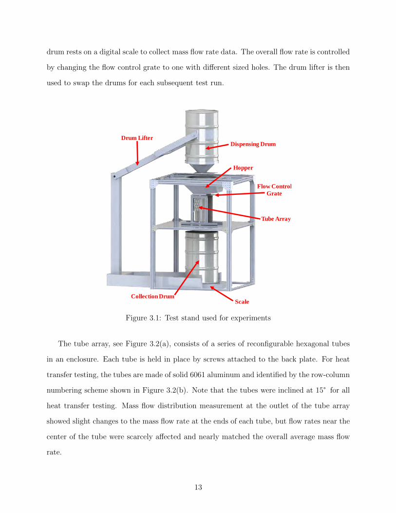
drum rests on a digital scale to collect mass flow rate data. The overall flow rate is controlled

by changing the flow control grate to one with different sized holes. The drum lifter is then

used to swap the drums for each subsequent test run.

Dispensing Drum

Collection DrumScale

Tube Array

Hopper

Drum Lifter

Flow ControlGrate

Figure 3.1: Test stand used for experiments

The tube array, see Figure 3.2(a), consists of a series of reconfigurable hexagonal tubes

in an enclosure. Each tube is held in place by screws attached to the back plate. For heat

transfer testing, the tubes are made of solid 6061 aluminum and identified by the row-column

numbering scheme shown in Figure 3.2(b). Note that the tubes were inclined at 15° for all

heat transfer testing. Mass flow distribution measurement at the outlet of the tube array

showed slight changes to the mass flow rate at the ends of each tube, but flow rates near the

center of the tube were scarcely affected and nearly matched the overall average mass flow

rate.

13

Internal cartridge heaters are used to heat the middle 3 rows to simulate solar flux. The

top row is unheated and serves to establish a steady state flow pattern over the heated

tubes. Only partial tubes are used in the bottom row. These are again unheated and serve

to maintain the proper flow pattern along the bottom face of the last row of heated tubes.

Partial tubes are used for their lower heat capacity to limit heat loss from the already heated

sand. Half tubes are used on the sides to maintain consistent flow.

Glass Sides

Unheated Top Row

Heated Central Rows

Partial Bottom Row

Back Plate

Instrumented

Tube (3-3)

(a) Heated tube array (b) Tube numbering scheme

Figure 3.2: Instrumented tube setup used for experiments

Each heated tube is configured as shown in Figure 3.3 with the dimensions shown in

Figure 3.4. A cartridge heater extends the full length of the tube. The heaters are manu-

factured by Watlow and rated for 1 kW of power for each full tube and 500 W for each half

tube. Each heater has an internal thermocouple for measuring the heater temperature and

an additional thermocouple is inserted into a small hole in the tube body to measure the

overall average temperature of the tube. An insulating gasket is placed between the surface

of the tube and both the back plate and front glass to limit heat transfer from the ends of

the tube. An additional rubber strip is placed between the insulating gasket and the front

glass to hold the tube in place and prevent particles from flowing between the tube and glass.

Additional insulation is placed around the outside of the tube array to limit heat losses.

14

Figure 3.3: Single heated tube cross-sectional diagram

SectionpA-A

0.47"

0.47"

0.47"

SectionpA-A

90°

1.18"

HeaterpHole3/8"pDIA

TCpHole0.05"pDIA

A

A

9.84"

15°

0.65"

1.67"

Spacing

Figure 3.4: Dimensions of heated tubes used in experiments

In addition to the central thermocouple, one tube, located at position 3-3, has been

outfitted with additional thermocouples for measurement of local temperatures as shown in

Figure 3.5. Grooves were machined partway down the length of the tube at each vertex and

along the center of each face. One thermocouple is embedded in each of these grooves and

covered with thermal cement. These thermocouples serve to measure the local temperatures

along the surface of the tube. A second thermocouple runs along each groove before extending

into the flow to measure the local particle temperature. This is done by a gentle curve to

avoid working the metal and distorting the thermocouple readings.

Thermocouples are also placed above and below the tube array to capture the inlet and

outlet particle temperatures. Two inlet thermocouples are embedded within the incoming

15

TC for Particle

Flow Temperature

Measurement

TC Covered with

Thermal Cement for

Surface Temperature

Measurement

Figure 3.5: Instrumented tube for “local” heat transfer measurements

sand that collects on the flow control grate. One outlet thermocouple is placed in the center of

a funneling device designed to gather and mix the outlet particles for an average reading. An

additional outlet thermocouple is embedded in the particles as they collect in the collection

drum. All thermocouples are sheathed, stainless-steel K-type thermocouples from Omega as

detailed in Table 3.1.

Table 3.1: Specifications of thermocouples used in experiments

TC Location Type Diameter LengthTube Center K 1/16” 6”

Instrumented Tube K 0.040” 12”Inlets and Outlets K 0.040” 12”

3.2.1 Electrical Control System and Data Acquisition

The heaters are powered through the custom electrical control box shown in Figure 3.6(a).

Three-phase 240 Volt electrical power is supplied to the box and runs through a contactor

switch. This switch controls the flow of electricity to the box for emergency shutoff purposes.

Each phase is then split and the heaters are connected evenly between each pair of phases.

16

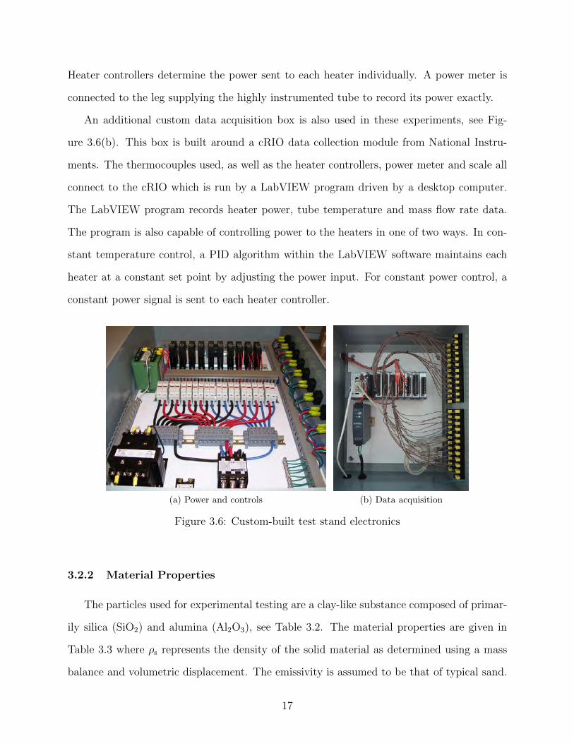
Heater controllers determine the power sent to each heater individually. A power meter is

connected to the leg supplying the highly instrumented tube to record its power exactly.

An additional custom data acquisition box is also used in these experiments, see Fig-

ure 3.6(b). This box is built around a cRIO data collection module from National Instru-

ments. The thermocouples used, as well as the heater controllers, power meter and scale all

connect to the cRIO which is run by a LabVIEW program driven by a desktop computer.

The LabVIEW program records heater power, tube temperature and mass flow rate data.

The program is also capable of controlling power to the heaters in one of two ways. In con-

stant temperature control, a PID algorithm within the LabVIEW software maintains each

heater at a constant set point by adjusting the power input. For constant power control, a

constant power signal is sent to each heater controller.

(a) Power and controls (b) Data acquisition

Figure 3.6: Custom-built test stand electronics

3.2.2 Material Properties

The particles used for experimental testing are a clay-like substance composed of primar-

ily silica (SiO2) and alumina (Al2O3), see Table 3.2. The material properties are given in

Table 3.3 where ρs represents the density of the solid material as determined using a mass

balance and volumetric displacement. The emissivity is assumed to be that of typical sand.

17

Table 3.2: Composition of particles used in experiments

Compound CompositionSiO2 50-55%

Al2O3 40-45%Fe2O3 0.7-1.7%TiO2 2.0-2.75%K2O trace-1.5%MgO trace-0.7%CaO trace-0.5%Na2O trace-0.5%P2O5 trace-0.71%

Table 3.3: Properties of particles used in experiments

Parameter Symbol ValueMaterial density ρs 2700 kg/m3

Emissivity ep 0.8

Two batches of these particles were used for experiments as differentiated by their particle

size distributions, see Figure 3.7. The 200 µm batch contains particles ranging from roughly

50 µm up to 400 µm centered at 200 µm. The 300 µm batch is more tightly controlled to

particles ranging from approximately 150 µm up to 400 µm centered at 300 µm and is more

representative of the particles expected to be used in an operational receiver.

0

0.2

0.4

0.6

0.8

1

1.2

0 100 200 300 400 500 600

Cumulative Fractio

n

Particle Diameter (μm)

300 μm batch

200 μm batch

Figure 3.7: Particle batch sieve curves

18

3.3 Heat Transfer Testing Procedure

Heat transfer experiments were conducted by first heating the tubes to a constant tem-

perature. Control of the tubes was then switched to constant power while particle flow was

started simultaneously. This generated a first order decrease in the temperature of each

tube towards a steady state value. The flow rate was sufficient to exhaust the entire 200

kg particle supply in as little as 1-2 minutes. Efforts to control for constant temperature

during particle flow showed slow response times and were ineffective over the short time of

experimentation. Constant power control proved much more effective as long as the starting

temperature was above the steady state temperature for each tube. The tubes still did not

reach steady state temperature, but the first order nature of the resulting signal allows for

extrapolation to steady state values using an equation of the form

Tt = C1eC2t + C3 (3.1)

where C1, C2 and C3 are constants.

3.3.1 Average Heat Transfer Data Analysis

The data was analyzed by first extracting the relevant data from the full data set. This

includes the data from just after the flow starts to just before it ends. From the data it is also

clear that a steady state was not reached during testing. In order to extrapolate to steady

state values, the temperature data for each tube over this time frame was fit to Equation

3.1 using MATLAB.

A sample of the relevant raw data for the test duration is shown in Figure 3.8(a) and the

corresponding fit data is shown in Figure 3.8(b) according to the tube numbering scheme in

Figure 3.2(b). It should be noted that the wide range of steady state temperatures is typical

of results. This is believed to be due to the erratic nature of the flow. Some tubes experience

more particle contact than others which leads to different heat transfer characteristics for

each tube.

19

0 20 40 60 8090

100

110

120

130

140

150

160

time (sec)

Tub

e T

empe

ratu

re (

C)

2−12−22−33−13−23−33−44−14−24−3

(a) Raw data

0 50 100 15090

100

110

120

130

140

150

160

time (sec)

Tub

e T

empe

ratu

re (

C)

2−12−22−33−13−23−33−44−14−24−3

(b) Exponential fit

Figure 3.8: Sample tube temperature results

Sample data for the particle temperatures is shown in Figure 3.9(a) and for the input

power in Figure 3.9(b). Note that tubes 3-1 and 3-4 are half tubes which contain smaller

heaters and receive half the power of the others.

0 20 40 60 8022

24

26

28

30

32

time (sec)

Par

ticle

Tem

pera

ture

(C

)

Inlet 1Inlet 2Outlet 1Outlet 2

(a) Particle temperature

0 20 40 60 80150

200

250

300

350

400

450

500

time (sec)

Hea

ter

Pow

er (

W)

2−12−22−33−13−23−33−44−14−24−3

(b) Heater power

Figure 3.9: Sample particle temperature and power input results

Only the power supplied to tube 3-3 was explicitly measured by a power meter, the others

must be inferred. To do this, the voltage applied to the heater in tube 3-3 is back calculated

from the measured power, known heater resistance and the recorded heater duty cycle sent

to the controller. As the heaters are connected to a single power source and in the same

20

configuration, the applied voltage was assumed to be the same for all heaters. This was also

verified through direct measurement. The calculated applied voltage was then used with the

known resistance and the recorded duty cycle of each other heater to calculate the individual

power inputs.

This method proved more accurate than using an energy balance between the inlet and

outlet particle temperatures to determine power input as the precision of the thermocouples

over a temperature increase of only a few degrees Celsius is prohibitive. The average power

input to each tube was calculated by averaging the power input over the duration of the

test. The average mass flow rate was calculated by taking the slope from a linear fit of the

mass versus time data. The inlet and outlet particle temperatures were found by taking the

average over the second half of the test duration. An average particle temperature for each

row was found by dividing the change in temperature from the inlet to the outlet by the

number of heated rows and assuming a linear increase by row.

Once the steady state values were determined, the average heat transfer coefficient, h,

for each tube was calculated by

h =qh

At (Tt − Tp)(3.2)

where qh is the heater power, Tt is the tube surface temperature, Tp is the particle flow

temperature and At is the surface area of a single tube. An average heat transfer coefficient

for each test run was then obtained by averaging the values for each tube.

3.3.2 “Local” Heat Transfer Coefficient Analysis

The average heat transfer coefficient (HTC) for each face was found by first extracting the

steady state surface temperature results for tube 3-3 using the same exponential fit method

described above. The heat transfer coefficient cannot be calculated directly as the heat

flux through each face is unknown. Instead, a model was created to simulate heat transfer

within the system using ANSYS Fluent. A 2D cross section of the solid tube geometry was

constructed and is shown with the boundary conditions applied in Figure 3.10.

21

Figure 3.10: Fluent setup and boundary conditions for “local” heat transfer coefficients

The heat transfer was assumed to be a constant value across each face. A User-Defined

Function (UDF) was created to update the average heat transfer coefficient for each face until

the center temperature for each face matched the experimental results. Face temperatures

input into the UDF were obtained by averaging the experimental results between the two

sides of the tube to maintain symmetry. The heat flux boundary was set by dividing the

total heater power by the surface area of the heater bore hole. The ambient temperature

was set using the average particle temperature for the tube row instead of the temperatures

measured by the thermocouples protruding into the flow due to inconsistencies in the data

collected. For some surfaces, it was unknown if the thermocouples were even measuring the

particle temperature or were instead measuring the air temperature as the exact location of

the thermocouple tip could not be observed during testing. A sample of the Fluent results

compared to the experimental data is shown in Figure 3.11 where the three data points at

the center faces used as the input values to Fluent are indicated. The results match very

well except for the two endpoints which correspond to the top and bottom vertexes of the

hexagonal tube.

22

364

366

368

370

372

374

376

0 0.01 0.02 0.03 0.04 0.05 0.06

Tempe

rature [K

]

Location Along Perimeter [m]

Fluent ResultsExperimental DataInput Values

Figure 3.11: A sample of Fluent temperature results along the side of a single tube from topto bottom vertexes compared to experimental data

3.4 Results

The average heat transfer coefficient (HTC) results for both particle batches tested are

shown in Figure 3.12 where each point represents the average of the individual h values

measured for a single test. The mass flow rate has been normalized for consistency with

numerical results that will be discussed in Chapter 4. It can be seen that the heat trans-

fer coefficient is improved with increasing mass flow rates, as well as slightly improved by

increased heater power for a given mass flow rate. The 200 µm particle batch displays a sig-

nificantly higher HTC for a given mass flow rate. The highest mass flow rate shown for each

particle batch represents the highest achievable flow rate through the constructed geometry.

Lower flow rates are achieved through the use of rate limiting flow control grates and higher

values can not be achieved without changing the tube spacing.

The “local” heat transfer coefficient results for each face for the 300 µm particle batch

are shown in Figure 3.13 and for the 200 µm batch in Figure 3.14. For the 300 µm batch, the

top tube surface shows a considerably higher average HTC than the other faces except for at

the lowest flow rate tested where it matches the side face value. The bottom surface exhibits

minimal heat transfer while the side face heat transfer coefficient is roughly half that of the

top face for higher mass flow rates. Increasing the mass flow rate shows an increase in the

23

0

50

100

150

200

250

0.00 0.10 0.20 0.30 0.40 0.50

Avg He

at Transfer C

oefficien

t [W

/m^2

‐K]

Mass Flow Rate [kg/s/half‐tube channel]

300 µm 340 W 300 µm 425 W 300 µm 515 W 200 µm 340 W 200 µm 425 W

Particle Batch

Powerper tube

Figure 3.12: Average heat transfer coefficient results

050100150200250300350400450

0.00 0.10 0.20 0.30 0.40 0.50

Heat Transfer C

oefficient

[W/m

^2‐K]


BottomSideTop

Tube Face

Figure 3.13: Local heat transfer coefficient results by face for the 300 µm particle batch

0

100

200

300

400

500

600

0.00 0.10 0.20 0.30 0.40 0.50

Heat Transfer C

oefficien

t[W

/m^2

‐K]


BottomSideTop

Tube Face

Figure 3.14: Local heat transfer coefficient results by face for the 200 µm particle batch

24

HTC for all faces with the exception of a dip in the side face heat transfer for moderate mass

flow rates.

Results for the 200 µm particle batch show that the increase in the average heat transfer

coefficient due to decreases in particle size is mostly due to increases for the top tube face.

The side and bottom heat transfer coefficients show slight decreases. Results were not

obtained at different flow rates.

3.4.1 Flow Visualization

Additionally, video recording of particle testing was conducted during several unheated

test runs. A sample of these results at maximum flow conditions for the inclined tubes tested

is shown in Figure 3.15(a). From this image we can see that there are significant differences

in the flow patterns between different channels. It can also be seen that the flow over the

top tube faces typically does not fill the entire channel while the vertical flow channels are

packed. Some of the packing is due to the previously mentioned effect of the inclination

angle on the flow at the ends of the tubes and some due to wall effects.

(a) 15° inclined tubes (b) Horizontal tubes (image courtesy of NREL andOhio State University)

Figure 3.15: Particle flow visualization results

25

Previous testing on a smaller assembly of horizontal tubes, see Figure 3.15(b), shows

flow patterns more characteristic of flow at the center of the tube where the heat transfer

measurements took place. Here the particle flow along the top tube surface is characterized

by a significant gap between the surface of the particle flow and the under side of tube above.

The depth of this flow decreases along the length of the tube face. The vertical channels

are not packed as full as the inclined tube case but are still mostly filled. Flow between

each channel is unique for both the vertical and inclined portions and displays significant

variability.

3.5 Results Discussion

The observed increase in overall heat transfer with increasing mass flow rate is consistent

with the previously reviewed literature and is largely due to the increased thermal mass of

increased particle flow. Decreasing the particle diameter also increased overall heat transfer

as anticipated by previous literature studies. This came at the cost of decreased mass

flow, however. Lastly, increasing the heater power leads to a slight increase in heat transfer

coefficients as well. This is believed to be due to a slight increase in radiation effects caused by

the increased temperatures of the tube surfaces. Overall, the effects of radiation are largely

negligible in the low temperature range studied and the coefficients measured represent

mostly convective heat transfer.

Coupling particle flow visualization with the “local” heat transfer results shows that

particle contact correlates with the heat transfer coefficients. The top face is observed to

have particle contact over its entire length and a significantly higher heat transfer coefficent.

The bottom face has no particle contact and a poor heat transfer coefficient while the side face

is observed to have slight flow separation from the wall with intermittent particle contact and

a moderate heat transfer coefficient. It is also observed that the flow in the vertical channels

and the depth of the flow across the top surfaces are highly variable. This variability in flow

patterns between tubes likely plays a significant role in the observed variability in the heat

transfer coefficients.

26

CHAPTER 4

MODELING APPROACH

In order to expand the results of the heat transfer testing beyond the narrow range of

operating conditions examined and for use in overall receiver design analysis, a numerical

model for the NBB receiver was developed using MATLAB. This model predicts tube and

particle temperatures for a full-sized receiver by incorporating both heat transfer from the

heated tubes to the particles and radiative heat transfer internal to the tubes and to the sur-

roundings. This is done through the use of simplified 1D modeling of the cascading granular

flow which evaluates flow parameters relevant to heat transfer characteristics. These param-

eters are then used in conjunction with heat transfer correlations specific to each surface

of the hexagonal tube array to calculate effective heat transfer coefficients. The simplified

nature of the model allows for a full-sized receiver consisting of hundreds of rows of tubes to

be simulated in a reasonable time frame while showing agreement with experimental data.

This is a significant improvement over previous modeling efforts. The modeling approach

and the equations used are further discussed in the following chapter.

4.1 Modeling Methodology

For analyzing the NBB receiver design, only a narrow vertical section must be examined

due to symmetry in the horizontal direction. The domain is then discretized into nodes

that contain tubes and those that contain flowing particles. The thin segment used for this

analysis is shown in Figure 4.1 along with the repeating unit cell discretized into nodes. It is

useful to distinguish between node types because they are governed by different equations.

Analysis is conducted on a one-dimensional basis that neglects changes in parameters along

the length of the tube. The final program operates according to the flow chart shown in

Figure 4.2.

27

Low

er

Par

ticle

Flow N

odes

Tube

Nodes

Upper

Tube

Nodes

Figure 4.1: Discretized domain used for modeling

Input Solver and Discretization Settings

Calculate Derived Variables

Run

Input Initial Variables and Constants

Create Arrays for Tube and Flow Data

Initialize Outputs

Update h_eff Using Current Data

Calculate Tube Temperatures

Calculate Particle Flow Parameters

Check for Temp Convergence

Summarize Data & Create Graphs

Yes

No

Figure 4.2: MATLAB program flow chart

The initial parameters, such as the inlet temperature and mass flow rate, can be set

by the user. Once program operation commences, values for each particle flow and tube

node are initialized based on these inputs. The state variable for each tube node is the

tube temperature. For each particle flow node, there are five: particle temperature, particle

velocity, gas velocity, solids volume fraction and particle flow depth. The gas temperature is

assumed to match the particle temperature and is therefore not included as a state variable.

28

An effective heat transfer coefficient that includes both convection and radiation effects can

then be calculated between each tube wall and the adjacent particle flow based on these

state variables.

The tube temperatures are calculated using an energy balance for each node. This is done

by matrix inversion assuming a constant particle temperature for each node. The particle

flow state variables are then calculated by solving a mass balance on the gas flow and mass,

momentum and energy balances on the particle flow. These are solved simultaneously using

fsolve, one of MATLAB’s built in non-linear equation solvers, and the tube temperatures and

heat transfer coefficients from the previous iteration. The effective heat transfer coefficients

are then updated using the new values for all nodes before the process is repeated. Iteration

continues until the change in temperature of all nodes between iterations meets a desired

residual criteria.

4.2 Tube Wall Equations

qparticles

qconduction

qreradiation

qsolar

qconduction

x

y

Control

VolumeReradiationto all nodes

Figure 4.3: Control volume used for tube wall nodes with energy flows

The temperature of each tube node is calculated by evaluating an energy balance for each

node that includes incoming solar radiation, conduction between adjacent nodes, convection

and radiation to the flowing particles and reradiation inside each tube as shown in Figure 4.3

29

and Equation 4.1.

q = −kt

(∂2Tt

∂x2

)(4.1)

where kt is the conductivity of the tube material, Tt is the tube wall temperature, x is the

direction parallel to the tube surface and q is the net, volumetric energy input which includes

incoming solar flux, outgoing reradiation and heat transfer to the particles. This equation

is discretized to give

q′′

solardxLt = ttLtkt

dx(2Tt,i − Tt,i−1 − Tt,i+1) + dxLtheff (Tt,i − Tp) + dxLtq

′′

reradiation (4.2)

where tt is the thickness of the tube wall, Lt is the length of the tube, heff is the effective

heat transfer coefficient between the tube surface and particle flow and Tp is the particle

temperature adjacent to the surface. The reradiation from a node i to all other nodes and

to the ambient is found using

q′′

reradiation =n∑j=1

Fi,jσein

(T 4

t,i − T 4t,j

)(4.3)

where ein is the emissivity of the tube’s inner surface, σ is the Stefan-Boltzmann constant

and the view factors, Fi,j, are found using 3-D view factor relations between nodes and by

utilizing the enclosure rule for the view factor to the ambient. Although the vertical column

of the NBB receiver under consideration only includes half the nodes for a given tube,

radiation to the entire tube is simulated by including “phantom” nodes that are assumed to

be at the same temperature as their mirrored partners. It is further assumed that the back

wall of the receiver tube does not participate in radiation exchange and that heat transfer

to the ambient is through reradiation only.

4.2.1 Tube Wall Conductivity

The conductivity of the tube wall is assumed to be that of stainless steel. Changes in

conductivity with temperature are given by

kt = 14.6 + 0.0127Tt (4.4)

30

where Tt is given in °C and kt in W/m-K [43].

4.2.2 Radiation View Factors

Each hexagonal tube is discretized into long, rectangular segments which can be consid-

ered finite, three-dimensional planes. The view factor between any two of these segments

can then be calculated using the proper view factor relation and geometric parameters.

A (0,0)

90 −𝛼

2

𝛼

𝛽B

D

C

𝜃 = 90 +𝛼

2𝛼

𝐿𝑡𝑜𝑝

𝐿𝑠𝑖𝑑𝑒

𝐿𝑏𝑜𝑡𝑡𝑜𝑚 x

y

Figure 4.4: Tube input dimensions

The tube geometry is input using the dimensions shown in Figure 4.4 and the tube length.

The view factor between any two arbitrary nodes is calculated by first using their coordinates

to determine their relative position to one another. The appropriate view factor relation can

then be selected. Lastly, the necessary geometric constraints are calculated based on the

node locations and used in the proper equation.

There are three potential view factor configurations in the current hexagonal tube design,

as discussed below. Although much of the modeling is performed on a 1D basis, the radiative

heat transfer is calculated using view factors based on the 3D geometry of the tube and

includes the dimensions shown in Figure 4.4 as well as the length of the tube. The view

factor equations come from the 3rd edition of the Catalog of Radiation and Heat Transfer

Configuration Factors [44].

31

Offset Parallel Planes

Figure 4.5: Offset parallel planes configuration

For two nodes that are on directly opposed faces, the offset parallel planes view factor

relation shown in Figure 4.5 can be used. The view factor is then calculated by

F1−2 =1

(x2 − x1) (y2 − y1)

2∑i=1

2∑j=1

2∑k=1

2∑l=1

(−1)i+j+k+lG (xi, yj, bk, al) (4.5)

where

G =1

2π

[(y − b)

√(x− a)2 + z2 tan−1

(y − b√

(x− a)2 + z2

)

+ (x− a)√

(y − b)2 + z2 tan−1

x− a√(y − b)2 + z2

−z

2

2ln((x− a)2 + (y − b)2 + z2

)](4.6)

32

Contacting Planes

Figure 4.6: Contacting planes view factor diagram

For the case of two nodes that meet at a corner of the tube, the view factor can be

determined by considering the nodes to be two contacting rectangular planes as shown in

Figure 4.6. Using the dimensions shown, the view factor can be calculated by

F1−2 = − sin 2φ

4πB

[AB sinφ+

(π2− φ

) (A2 +B2

)+B2 tan−1

(A−B cosφ

B sinφ

)+A2 tan−1

(B −A cosφ

A sinφ

)]+

sin2 φ

4πB

{(2

sin2 φ− 1

)ln

[(1 +A2

) (1 +B2

)1 + C

]+B2 ln

[B2 (1 + C)

(1 +B2)C

]+A2 ln

[A2(1 +A2

)cos 2φC (1 + C)

cos 2φ

]}

+1

πtan−1

(1

B

)+

A

πBtan−1

(1

A

)−√C

πBtan−1

(1√C

)+

sinφ sin 2φ

2πBAD

[tan−1

(A cosφ

D

)+ tan−1

(B −A cosφ

D

)]+

cosφ

πB

∫ B

0

√1 + ζ2 sin2 φ

[tan−1

(ζ cosφ√

1 + ζ2 sin2 φ

)+ tan−1

(A− ζ cosφ√1 + ζ2 sin2 φ

)]dζ

(4.7)

where

A = a/c (4.8)

B = b/c (4.9)

C = A2 +B2 − 2AB cosφ (4.10)

D =(1 + A2 sin2 φ

)2(4.11)

33

Adjacent Planes

Figure 4.7: Adjacent planes diagram

The remainder of node pairs on any two arbitrary faces can be considered two nodes on

adjacent, non-contacting faces as shown in Figure 4.7. The vertex where the two planes meet

is not necessarily located on the tube perimeter and must be determined from the location

of the nodes. The view factor between the areas of interest, A1 to A4, can be calculated by

F1−4 =A1 + A2

A1

(F12−34 − F12−3)− A2

A1

(F2−34 − F2−3) (4.12)

where F12−34, for example, denotes the view factor from the entire upper plate to the entire

lower plate. The intermediate steps are evaluated using the contacting planes relation in

equation 4.7.

4.3 Heat Transfer Correlations

For the hexagonal geometry under consideration, no single heat transfer correlation from

the literature is sufficient for predicting heat transfer from the receiver tubes to the flowing

particles, especially when knowledge of the heat transfer for each face is needed. Instead,

each face is treated individually. The top face is considered an angled flat plate with good

particle contact, the side faces are treated as vertical plates or channels and the bottom

face is treated by considering air moving through the gap between the tube surface and the

air-particle interface.

34

4.3.1 Top Face

The most developed and useful correlation for heat transfer in gravity-driven granular

flows down inclined plates comes from the work of Patton [30]. The Nusselt number for such

a flow is given by

Nu∗d =hdp

kg

=1

xeff +(√

π2

)(1√Pe∗L

)(1 + β Fr∗√

Pe∗L

) (4.13)

where h is the average heat transfer coefficient, dp is the particle diameter and kg is the

gas phase conductivity. xeff defines the “effective” film thickness and is dependent upon the

geometry of the particles and the surface. A value of xeff = 0.065 was found to apply to

most smooth surfaces [30] and was used here. β is an empirical constant. A value of β = 15

is recommended [30] and was used here. The Nusselt number is also a function of Fr∗ and

Pe∗L, which are the modified Froude and Peclet numbers, respectively. They are defined by

Fr∗ =v2

gd cos(θ)

εcε

k

kg

dp

L(4.14)

Pe∗L =

(k

kg

)2(dp

L

)2vL

α(4.15)

where L is the plate length, θ is the inclination angle of the plate as measured from horizontal,

ε is the solids volume fraction of the flowing media, εc is the critical solids volume fraction

which was taken to be 0.56 as recommended [30], k is the bulk conductivity of the particle

phase, v is the average flow velocity, d is the depth of the flowing media and α is the bulk

thermal diffusivity of the particle phase defined by α = kρcp

where cp is the particle phase

specific heat and ρ is the bulk density of the flowing media given by ρ = ρsε.

4.3.2 Side Face

Of the work pertaining to granular flows in vertical channels, the correlation of Sullivan

and Sabersky [28] is most applicable to the side walls of the hexagonal geometry. This is

due to the smooth walled channels used in their experiments as well as the development of

35

a simple correlation for the Nusselt number which is given by

Nu∗d =hdp

kg

=1

xeff +√π

2

√1

Pe∗L

(4.16)

where the Peclet number is again given by equation 4.15 and xeff again represents the “effec-

tive” film thickness. A value of xeff = 0.085 was found to give the best fit to the experimental

data for vertical channels [28].

As discussed previously, this correlation was developed using data from plug flow exper-

iments in a long vertical channel. Although similar, this differs noticeably from our flow

regime where the particles are in free fall and not completely packed. Experiments also show

that the particles do not maintain consistent contact with the side walls. In order to modify

this correlation to fit our flow regime, the “effective” film thickness is increased to account

for conduction through a larger gap between the walls and particles. The exact value used

will be discussed further in Section 4.5.

4.3.3 Bottom Face

Experiments have shown that there is little to no contact between the particle flow and

the bottom surface of the receiver tubes. Therefore, a heat transfer correlation was developed

by considering air flow through the thin channel formed by the upper surface of the particle

flow and the bottom face of the tube. The bottom tube surface is considered to be a constant

flux boundary due to the solar flux incident on the solar side of the tube. The air-particle

interface is treated as an insulated boundary by assuming the air and particles to be at

the same temperature. The average Nusselt number for fully developed flow through a thin

channel with these boundary conditions is given by [45, 46]

NuD =hDh

kg

= 5.39 (4.17)

where h is again the average heat transfer coefficient, kg is the gas phase conductivity and Dh

is the hydraulic diameter of the channel given by Dh = 4tL2W+2t

where W is the channel width

and t is the channel thickness. In the case of our geometry, the channel width is defined by

36

W = Lt, the length of the tube, and the air channel thickness is defined by t = H − d where

H is the total height of the channel and d is the depth of the particle flow.

For the short face under consideration, the flow is not fully developed, however. The

dimensionless axial distance along the tube for developing flow is given by [46]

x∗ =x

DhRePr(4.18)

where Re and Pr are the Reynolds and Prandtl numbers for the flowing gas and x is the

distance along the channel. Values of roughly x∗ < 0.25 have significant entry length effects.

Tabular values for the local Nusselt number, Nux, have been found for fluid flow between

parallel plates with one at constant flux and the other insulated for various x∗ and Pr values

[46]. An equation was developed for the range of 0.001 < x∗ < 0.025 and 0.01 < Pr < 10 by

curve fitting the tabular data as shown in Figure 4.8.

y = 1.364x‐0.411R² = 0.9953

y = 1.6221x‐0.345R² = 0.9872

y = 1.9894x‐0.294R² = 0.9935

0

5

10

15

20

25

30

0 0.005 0.01 0.015 0.02 0.025

Local N

usselt Num

ber [Nu x]

Dimensionless Axial Distance [x*]

Pr = 0.01

Pr = 0.70

Pr = 10.0

(a) Nusselt number vs x∗

y = 0.0112x2 + 0.1163x + 1.6622R² = 1

y = ‐0.0005x2 ‐ 0.0182x + 0.3386R² = 1

0

0.5

1

1.5

2

2.5

‐5 ‐3 ‐1 1 3

Power Fit Co

efficients

ln(Pr)

A coefficient B coefficient

(b) Coefficients vs Pr

Figure 4.8: Development of Nusselt number fit curve

Nux was fit to an equation of the form Nux = A (x∗)-B and the resulting A and B

coefficients were fit to an equation of the form y = C1 (ln Pr)2 + C2 (ln Pr) + C3. The

resulting equation for the local Nusselt number is given by

Nux = A (x∗)-B (4.19)

37

where

A = 0.0112 (ln Pr)2 + 0.1163 (ln Pr) + 1.6622 (4.20)

B = −0.0005 (ln Pr)2 − 0.0182 (ln Pr) + 0.3386 (4.21)

The average Nusselt number for the bottom surface is then found by averaging over the

surface using

NuD =

∫ x∗0

Nuxdx

x∗(4.22)

The heat transfer from the bottom surface is then evaluated using the mean gas temper-

ature Tg given by

Tg =Tt + Tp

2(4.23)

4.3.4 Effective Heat Transfer Coefficient

In order to incorporate radiation while maintaining linear equations, an effective heat

transfer coefficient is used between the tube surfaces and the particle flow as shown below.

heff = hconv +σ(etT

4t − ecT 4

p

)Tt − Tp

(4.24)

where hconv is the convective heat transfer coefficient, Tt is the temperature of the adjacent

tube surface, Tp is the particle temperature, et is the emissivity of the adjacent tube surface

and ec is the emissivity of the particle curtain. The curtain emissivity differs from that of

the raw material due to changes in transmissivity and is calculated by [47]

ec = ep (1− τc) (4.25)

where τc is the transmissivity of the curtain given by

τc = exp

(− 3ε

2dp

zc

)(4.26)

where ε is the solids volume fraction of the particle curtain, dp is the particle size and zc is

the curtain thickness defined by the depth of the flow, d.

38

4.3.5 Particle Phase Conductivity

The bulk conductivity of the granular phase is an important parameter in many of the

correlations used for analysis. This can be calculated using the Maxwell model [48]

k =γkg (2kg + ks) + 3εkskg

γ (2kg + ks) + 3εkg

(4.27)

ε = 1− γ (4.28)

where k is the bulk conductivity of the granular phase, ks is the conductivity of the solid

material, kg is the conductivity of the interstitial gas phase, ε is the solids volume fraction

and γ is the gas volume fraction within the particle flow. This model gives the closest match

to experimental results using foundry sand of the models considered by Malherbe [48]. The

gas conductivity is that of air and is given in W/m-K using using Tg in Kelvin by

kg = 1.5207× 10−11T 3g − 4.8574× 10−8T 2

g + 1.0184× 10−4Tg − 3.9333× 10−4 (4.29)

4.4 1D Granular Flow Modeling

In order to calculate the parameters needed to predict the heat transfer coefficients, the

granular flow dynamics were also modeled. This was done by assuming one-dimensional

flow through the receiver section under consideration using control volumes as shown in

Figure 4.9. Although this appears to be a significant assumption, the existing literature on

granular flows over plates, as discussed in the literature review, concludes that the volume

fraction and velocity profiles through the depth of such a flow are nearly constant [38–40].

The parameters of interest are the solids volume fraction, the depth of the particle flow,

the average particle velocity, the particle temperature, the average gas velocity and the gas

temperature. In order to simplify the problem, it was assumed that the gas temperature

equals the particle temperature for a given node since the phases are highly intermixed and

both subject to heating. It was further assumed that the system operates under constant

pressure and air was treated as an ideal gas.

39

H

d

θ

v

vgControlVolume

Figure 4.9: Control volume for particle flow nodes with relevant variables and parameters

Other studies modeling granular flows down inclines treat the volume fraction as a con-

stant and allow the flow depth to change as the particles accelerate [41, 42]. This approach

was followed for the top tube surfaces. For the vertical channels, the experimental results

show that the particles spread out and do not have a well defined flow depth. For these

channels, it was assumed that the flow depth is equal to the height of the channel and the

average solids volume fraction was allowed to vary as the particles accelerate. The remaining

4 state variables were found using equations for conservation of mass, momentum and energy

for the particles and conservation of mass for the gas.

4.4.1 Solid Phase Continuity

The solid phase continuity equation at steady state takes the form

∂

∂x(ερsdv) = 0 (4.30)

where ε is the average solids volume fraction over the depth of the particle flow, v is the

average particle velocity parallel to the tube wall, d is the particle flow depth and ρs is the

density of the solids material. The bulk density is therefore defined by ρsε.

The discretized solids phase continuity equation for a control volume at node i can be

written

0 = ρsεi−1vi−1Ltdi−1 − ρsεiLtdivi (4.31)

40

where Lt denotes the length of the receiver tube and Ltd gives the cross-sectional area of the

particle flow.

4.4.2 Solid Phase Momentum

The solids momentum equation is given by

∂

∂x

(ερsdv

2)︸︷︷︸

momentum flux

= ερsdg sin θ︸︷︷︸gravity

− ερsdg cos θ tan δ︸︷︷︸wall friction

− dβv (v − vg)︸︷︷︸particle-air drag

(4.32)

where θ is the inclination angle of the surface from the horizontal, δ is the bed friction angle

which is defined as the minimum inclination angle needed for a layer of particles to flow over

the surface, vg is the gas velocity and βv is the drag coefficient. The drag coefficient can be

calculated from the Ergun equation [49, 50] by

βv = 150(1− γ)2 µg

γ (dpφs)2 + 1.75

ρg |vg − v| (1− γ)

φsdp

(4.33)

where µg is the gas viscosity, ρg is the gas density, dp is the particle diameter and φs is the

particle sphericity which is assumed to be unity. The gas viscosity is that of air and is given

in kg/s-m using Tg in Kelvin by

µg = 2.84450−6 + 5.9996× 10−8Tg − 2.6725× 10−11T 2g + 7.1510× 10−15T 3

g ; (4.34)

The discretized form of the momentum equation for a control volume becomes

0 = ρsLtdi−1εi−1v2i−1 cos (|θi−1 − θi|)− ρsLtdiεiv

2i

+ dxLtdiρsεig sin (θ)− tan(δ)dxLt (diρsεig cos (θ))− dxLtdiβv (vi − vg,i)(4.35)

where dx is the length of each node in the flow direction and the addition of cos (|θi−1 − θi|) on

the incoming solids momentum accounts for losses due to inelastic collisions as the particles

change direction at the tube corners. When transitioning from an inclined channel to a

vertical channel the particles impact each other, and when transitioning back to an inclined

channel the particles impact the surface of the next tube. It should be noted that other

models of granular flow down inclines include an additional rate-dependent friction term

41

[41, 42]. This was neglected in this analysis because the direction changes throughout the

flow regime dominate the maximum velocity obtained.

4.4.3 Gas Phase Continuity

The gas phase continuity equation is written as

∂

∂x((H − εd) ρgvg) = 0 (4.36)

where H is the height of the particle flow channel and (H − εd) represents the gas volume

fraction throughout the entire channel volume. The channel height must be included because

it is not constant throughout the array.

The discretized form is written

0 = Lρg,i−1 (H − εdi−1) vg,i−1 − Lρg,i (H − εdi) vg,i (4.37)

where the gas density is calculated using the ideal gas law and the gas is again assumed to

be at the same temperature as the particles.

4.4.4 Solid Phase Energy

The solid phase, steady state energy balance is given by

cp∂

∂x(Tp) + q = 0 (4.38)

where cp is the average specific heat of the particles and q is the volumetric energy input.

This can be written for a control volume as

0 = Ltdi−1ρεi−1vi−1cpTp,i−1−LtdiρεivicpTp,i+heff,W1 (TW1 − Tp,i) dxLt +heff,W2 (TW2 − Tp,i) dxLt

(4.39)

where there is heat input from the walls above and below the given particle node denoted

by subscripts W1 and W2. The temperatures are those of the adjacent tube nodes and the

heat transfer coefficients are evaluated by the previously discussed correlations and include

both convective and radiative contributions.

42

The particle specific heat is taken to be that of pure silica which differs only slightly from

alumina over the temperature range of interest. An equation was developed based on data

found in [51] and is given by

cp = 138.5667(4.871 + 0.005365Tp − 100100T−2p ) (4.40)

where cp is given in J/kg-K using Tp in Kelvin

4.4.5 Inlet Conditions

The inlet conditions are established by first setting the particle mass flow rate. Particles

then enter as if from a hopper and are assumed to fill the entire volume of the channel along

the top face of the first tube at the set constant solids volume fraction. The initial particle

velocity is then calculated to realize the desired mass flow rate. Air fills the remaining volume

and enters at the same velocity as the particles.

4.5 Input Parameter Selection Based on Comparison to Experimental Data

Several of the parameters needed for the equations discussed above remain unknown.

These are the flowing solids volume fraction along the top tube face, the bed friction angle

and the “effective” film thickness for the side face. These values were selected through

comparison with the experimental data at maximum flow conditions for the 300 µm particle

batch. The model was set to simulate the experiments by using the parameters in Table 4.1.

These were chosen to mimic solid aluminum tubes operated at moderate power.

4.5.1 Particle Flow Depth Considerations

One of the important parameters that must be considered in validating the model is

the depth of the particle flow over the top surface of the tubes. The simulation results, see

Figure 4.10, show that the particles accelerate along the top tube surfaces and in the vertical

channels before decreasing in velocity at the corners. The particle flow depth follows the

inverse of the velocity along the top tube surfaces. In reality, the maximum height of the

particle flow is constrained by the physical dimensions of the system.

43

Table 4.1: Input parameters for comparison to experimental data

Parameter Symbol Input ValueMass flow rate per channel m 0.43 kg/s

Tube wall thickness tt 0.30 inTube inner wall emissivity et 0Particle material emissivity ep 0.8

Particle tube surface emissivity et 0.2Tube material conductivity kt 167 W/m-K

Particle diameter dp 300 µmParticle inlet temperature Tp,0 25°C

Solar flux q′′solar 440 W/m2

Tube rows R 5

10 20 30 40 500

0.2

0.4

0.6

0.8

1

velo

city

[m/s

]

Node (flow over 5 tubes)

(a) Particle velocity vs node

10 20 30 40 500

2

4

6

8

10

Dep

th o

f flo

w [m

m]


(b) Flow depth vs node

Figure 4.10: Sample results

As previously mentioned, see Figure 3.4, the distance between each tube face in the

experimental array is the same, but the simulation considers a channel containing only half

of a tube width. Therefore, the height of the vertical channel within the simulation is half

the height of the inclined channel along the top face. In order for the flow to fit within these

constraints, the flow along the top surface must fill less than half of the channel height when it

reaches the entrance to the vertical channel. The input parameters that affect the flow depth

are the solids volume fraction along the top face and the bed friction angle. Figure 4.11(a)

shows the limiting flow depth over the first tube where the flow is slower and Figure 4.11(b)

44

shows the flow depth at the end of the top face for a tube farther down the array where steady

state conditions have been reached as functions of the relevant parameters. The flow depth

decreases with increasing solids volume fraction and decreasing friction angle. The dashed

line shows the maximum height that can fit the geometry. Points below this line represent

possible solids volume fraction and friction angle combinations that could be selected.

0.15 0.2 0.25 0.3 0.350

2

4

6

8

10

12

Ste

ady

Sta

te M

inim

umF

low

Dep

th [m

m]

Solids Volume Fraction

Frict Angle = 5Frict Angle = 15Frict Angle = 25Frict Angle = 35Frict Angle = 45Max Depth

(a) Entrance region min flow depth

0.15 0.2 0.25 0.3 0.350

2

4

6

8

10

12

Firs

t Row

Top

Fac

eM

inim

um F

low

Dep

th [m

m]


Frict Angle = 5Frict Angle = 15Frict Angle = 25Frict Angle = 35Frict Angle = 45Max Depth

(b) Steady state minimum flow depth

Figure 4.11: Flow depth considerations at maximum flow conditions

4.5.2 Heat Transfer Considerations

The effective heat transfer coefficient across the side face as a function of the “effective”

film thickness is shown in Figure 4.12 along with the experimental data. The effective heat

transfer coefficient is taken from the simulation for direct comparison to the experimental

results that include all modes of heat transfer. The solid horizontal line represents the mean

of the experimental results and the dashed lines represent 1 and 2 standard deviations from

the mean. Simulations showed that only the “effective” film thickness has significant impact

on the side face HTC. Decreasing the “effective” film thickness increases this heat transfer

coefficient.

The bottom face heat transfer coefficient is dependent upon the solids volume fraction

and the bed friction angle as these impact the flow depth and therefore the thickness of

45

0.35 0.4 0.45 0.5 0.550

50

100

150

200

250

Effe

ctiv

e H

eat T

rans

fer

Coe

ffici

ent [

W/m

2 K]

effective film thickness

Simulation ResultsAvg Exp Data1 & 2 SD Lines

Figure 4.12: Side face heat transfer analysis vs the relevant parameters

the air channel along the bottom surface. Changes in heat transfer with these parameters

are shown in Figure 4.13 along with the average experimental value and lines for 1 and 2

standard deviations from the mean. Heat transfer increases with decreases in the solids

volume fraction and with increases in the bed friction angle.

0.15 0.2 0.25 0.3 0.350

10

20

30

40

50

60

70

Effe

ctiv

e H

eat T

rans

fer

Coe

ffici

ent [

W/m

2 K]


Frict Angle = 5Frict Angle = 15Frict Angle = 25Frict Angle = 35Frict Angle = 45Avg Exp Data1 & 2 SD Lines

Figure 4.13: Bottom face heat transfer analysis vs the relevant parameters

46

Heat transfer across the top surface is also impacted by the solids volume fraction and the

bed friction angle, see Figure 4.14. Here the heat transfer also increases with increased bed

friction angle, but unlike the bottom face, increases with increased solids volume fraction.

0.15 0.2 0.25 0.3 0.350

100

200

300

400

500

600E

ffect

ive

Hea

t Tra

nsfe

rC

oeffi

cien

t [W

/m2 K

]


Frict Angle = 5Frict Angle = 15Frict Angle = 25Frict Angle = 35Frict Angle = 45Mean Exp Data1 & 2 SD Lines

Figure 4.14: Top face heat transfer analysis vs the relevant parameters

4.5.3 Parameter Selection

The value of the “effective” film thickness affects the side face heat transfer coefficient only

and this heat transfer is scarcely affected by any other parameters. A value of xeff = 0.43 was

therefore chosen to best match the average heat transfer coefficient from the experimental

results. Figure 4.12 shows that any value in the range of 0.4-0.5 could feasibly be chosen.

In order to select the appropriate values for the bed friction angle and the solids volume

fraction, the particle flow depth and top and bottom heat transfer coefficients must all be

taken into account. This was done through the use of the mutli-layered contour plot shown in

Figure 4.15. The gray shaded areas represent those that are satisfactory according to the flow

depth considerations with the darker areas being more preferable. The requirements have

been set at d < 6 mm for the steady state flow and d < 1.1× 6 mm to give a 10% tolerance

for the first tube where the slower and more densely packed flow conditions may cause the

solids volume fraction to increase. The blue and red shaded areas represent the acceptable

47

regions for the heat transfer from the top and bottom surfaces, respectively, and are centered

about the mean. The darker area for each color represents values within ±10% of the average

experimental value and the lighter area represents ±15%. ±15% is approximately the 2σ

window for the top face but represents a much tighter tolerance on the bottom face. Where

all of the darker areas overlap, as outlined by the solid black lines, represents the best fit

window according to the data collected. This window is biased towards meeting the top

face value and includes the 15% deviation range for the bottom face heat transfer. The

exact values selected were ε = 0.25 and δ = 20° as these were found to give the best results

of those within the acceptable window. The acceptable range and the values selected are

further outlined in Table 4.2.

SolidsfVolumefFraction

Bed

fFric

tionf

Ang

lef[d

eg]

0.15 0.2 0.25 0.3 0.355

10

15

20

25

30

35

40

45

hfbottomffacef<15wfdeviation

hfbottomffacef<10wfdeviation

hftopffacef<15wfdeviation

hftopffacef<10wfdeviation

SSfflowfdepthf<6mm

Firstfrowfflowfdepthf<6.6mm

X

Figure 4.15: All considerations for parameter selection

Table 4.2: Acceptable parameter inputs based on comparison to experimental data

Parameter Symbol Acceptable Range Value ChosenSolids volume fraction ε 0.20− 0.30 0.25

Side face “effective” film thickness xeff 0.40− 0.5 0.43Bed friction coefficient δ 5°−25° 20°

48

4.6 Model Validation

A more thorough validation of the model can be performed through analysis of the

results incorporating the final parameters selected. As shown in Figure 4.16, the particle

flow depth decreases to the required 6 mm before reaching the first vertical segment and for

each subsequent vertical channel. Additionally, the flow depth decreases along each top tube

surface in agreement with the flow observed in the experiments.

Depth ≤ half channel height at entrance to vertical sections

Figure 4.16: Flow depth considerations

The heat transfer results can also be compared to the experimental data as a function of

mass flow rate. This is shown for the 300 µm particle batch in Figure 4.17 and for the 200

µm batch in both Figure 4.18 and Figure 4.19.

From the 300 µm batch we can see that the data is well represented by the simulation.

At the maximum flow rate, the simulation results match the average experimental results

very closely. The simulation accurately captures the slight decrease in heat transfer with

decreased mass flow rate for the bottom surface across the range examined. The decrease in

the top face heat transfer coefficient with decreasing flow rate is also captured by the model

except for the dramatic decrease at the lowest mass flow rate. Heat transfer from the side

face shows a dip at moderate mass flow rates before increasing to a value slightly less than or

equal to those seen at the highest mass flow rate. The simulation predicts a slight decrease

in heat transfer with decreasing mass flow rate that follows the average well but does not

49

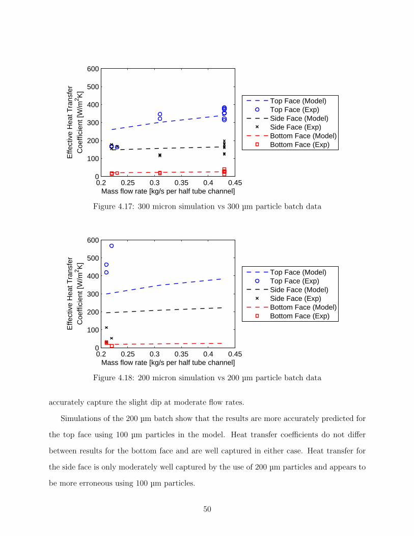
0.2 0.25 0.3 0.35 0.4 0.450

100

200

300

400

500

600

Mass flow rate [kg/s per half tube channel]

Effe

ctiv

e H

eat T

rans

fer

Coe

ffici

ent [

W/m

2 K]

Top Face (Model)Top Face (Exp)Side Face (Model)Side Face (Exp)Bottom Face (Model)Bottom Face (Exp)

Figure 4.17: 300 micron simulation vs 300 µm particle batch data

0.2 0.25 0.3 0.35 0.4 0.450

100

200

300

400

500

600


Effe

ctiv

e H

eat T

rans

fer

Coe

ffici

ent [

W/m

2 K]



accurately capture the slight dip at moderate flow rates.

Simulations of the 200 µm batch show that the results are more accurately predicted for

the top face using 100 µm particles in the model. Heat transfer coefficients do not differ

between results for the bottom face and are well captured in either case. Heat transfer for

the side face is only moderately well captured by the use of 200 µm particles and appears to

be more erroneous using 100 µm particles.

50

0.2 0.25 0.3 0.35 0.4 0.450

100

200

300

400

500

600


Effe

ctiv

e H

eat T

rans

fer

Coe

ffici

ent [

W/m

2 K]



4.7 Numerical Parameters

It is also important to discuss the numerical considerations of the model. The temperature

residual criteria governs convergence for the iterative solver and is defined by

∆Tres =Tc − Tprev

Tprev

(4.41)

where Tc is the current temperature value and Tprev is the value from the previous iteration

for a given tube or particle flow node temperature. The other important parameter is the

mesh sizing which is set by Nface, the number of nodes for each face of each tube. The results

for the particle outlet temperature and the maximum tube temperature vs Nface are shown

in Figure 4.20(a) and Figure 4.20(b) for three different temperature residual criteria from a

simulation of 30 rows of tubes and are representative of the trends seen in other parameters.

The ordinate is the normalized difference between the value for the given case and the value

predicted for Nface = 11 with ∆Tres = 1E-5.

These graphs show that the overall outlet temperature predicted by the model is scarcely

affected by the number of nodes as long as ∆Tres < 1E-4. Additionally, the maximum tube

temperature accuracy improves with increased node count but only moderately improves

51

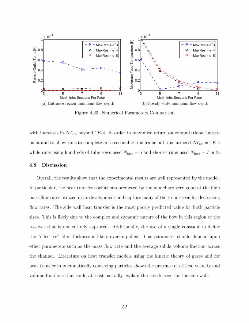
3 5 7 9 110

0.2

0.4

0.6

0.8

1x 10

−3

Mesh Info: Sections Per Face

Par

ticle

Out

let T

emp

[K]

MaxRes = e−3

MaxRes = e−4

MaxRes = e−5

(a) Entrance region minimum flow depth

3 5 7 9 110

0.2

0.4

0.6

0.8

1x 10

−3

Mesh Info: Sections Per Face

Max

imum

Tub

e T

empe

ratu

re [K

]

MaxRes = e−3

MaxRes = e−4

MaxRes = e−5

(b) Steady state minimum flow depth

Figure 4.20: Numerical Parameters Comparison

with increases in ∆Tres beyond 1E-4. In order to maximize return on computational invest-

ment and to allow runs to complete in a reasonable timeframe, all runs utilized ∆Tres = 1E-4

while runs using hundreds of tube rows used Nface = 5 and shorter runs used Nface = 7 or 9.

4.8 Discussion

Overall, the results show that the experimental results are well represented by the model.

In particular, the heat transfer coefficients predicted by the model are very good at the high

mass flow rates utilized in its development and capture many of the trends seen for decreasing

flow rates. The side wall heat transfer is the most poorly predicted value for both particle

sizes. This is likely due to the complex and dynamic nature of the flow in this region of the

receiver that is not entirely captured. Additionally, the use of a single constant to define

the “effective” film thickness is likely oversimplified. This parameter should depend upon

other parameters such as the mass flow rate and the average solids volume fraction across

the channel. Literature on heat transfer models using the kinetic theory of gases and for

heat transfer in pneumatically conveying particles shows the presence of critical velocity and

volume fractions that could at least partially explain the trends seen for the side wall.

52

The values chosen for the solids volume fraction and the bed friction angle represent the

best fit given the experimental data. As this data contains significant variability, the selected

parameters do not necessarily represent the exact physical parameters from the experiment.

A range of input parameters could have been selected that would fit the data within an

acceptable tolerance. More in-depth experiments could measure these parameters directly.

The heat transfer correlations developed make the inherent assumption of constant par-

ticle sizes. Comparison with experimental data shows that the presence of a mixture of

particle sizes can significantly vary the results. The 200 µm particle batch exemplifies heat

transfer characteristics more fitting of 100 µm sized particles. This is likely due to improved

contact at the particle surface due to the presence of fine particles within the particle batch.

This is not seen with the 300 µm particle batch as the particle size is more tightly controlled.

53

CHAPTER 5

RECEIVER ANALYSIS

The promising accuracy of the simplified model developed in the previous chapter gives

confidence in its use for analyzing the full-size receiver. The performance of the full system

can be analyzed using this model in a variety of ways. First, the equations developed,

such as the heat transfer correlations, can be analyzed directly to see the impact of various

parameters. Additionally, a full-sized receiver can be simulated at high temperature that

includes radiation on the solar side of the tubes and uses the expected operational parameters.

Temperatures and energy flows within the system can then be analyzed.

5.1 Heat Transfer Correlation Analysis

Here the primary parameters and variables that affect the heat transfer coefficients, the

particle flow depth, velocity and solids volume fraction, have been varied in order to study

the effects on the heat transfer correlations directly, see Figure 5.1. For these simulations

the gas velocity was set equal to the particle velocity. It should also be noted that these

simulations vary the parameters only and are not directly comparable between data points.

For example, increasing the velocity or solids volume fraction while maintaining a constant

velocity also leads to an increase in the average mass flow rate. Thus, the trends may be

examined but a given set of conditions may not be obtainable in the design.

From these graphs several trends can be observed for each of the faces. First, the bottom

face heat transfer is not directly dependent upon the solids volume fraction but does increase

slightly with both depth and gas velocity. Increased gas velocity increases the Reynolds

number, which leads to an increase in the entry length, and thus increases the average

Nusselt number and HTC for this face. The heat transfer coefficient is also dependent upon

the inverse of the air channel thickness, therefore, when the particle depth increases, the air

channel thins and the HTC increases.

54

Figure 5.1: Direct heat transfer correlation analysis results

The side face heat transfer correlation shows increases in the HTC with increases in both

velocity and solids volume fraction over the entire range of parameters studied. This is due

to the direct dependence of the Peclet number on the velocity and the particle phase con-

ductivity and the dependence of conductivity on the solids volume fraction. Increased solids

volume fraction decreases the distance between particles and improves bulk conductivity

leading to an improved HTC. The heat transfer coefficient from the side face has no direct

dependence on the particle flow depth.

The HTC for the top face is very dynamic over the range of parameters studied and is

significantly dependent upon each of them. The heat transfer coefficient for the top face

shows a maximum at a critical velocity that is unique for each set of other parameters. This

55

maximum is caused by the unique dependence of both the Peclet and Froude numbers on the

velocity. Largely due to the aforementioned improvements in particle phase conductivity, the

most significant increases in the HTC are caused by increasing the solids volume fraction.

Increasing the depth also increases the HTC as it decreases the Froude number.

5.2 Full Receiver Simulations

As previously mentioned, a significant advantage of this simplified model is its ability

to simulate a full-scale receiver. This was done using the input conditions and parameters

outlined in Table 5.1. These parameters incorporate the thin walls that would be needed for

a functional absorber tube and the temperature-dependent conductivity for stainless steel.

The particle side emissivity is set to that of stainless steel and the solar side is set for a

highly reflective material that would be needed to obtain appropriate solar flux spreading

along the length of the tube. The solids volume fraction, bed friction angle and side wall

“effective” film thickness utilize the parameters developed in the preceding chapter.

Table 5.1: Input parameters used for full NBB receiver simulation

Parameter Symbol Input ValueSolids volume fraction ε 0.25

Side face “effective” film thickness xeff 0.43Bed friction coefficient δ 20°Solids mass flow rate m 0.5 kg/sTube wall thickness tt 1/16 in

Solid particle material density ρs 2700 kg/m3

Solid particle material conductivity ks 1.5 W/m-KTube solar side emissivity ein 0.15

Tube particle side surface emissivity et 0.8Particle material emissivity ep 0.8

Particle diameter dp 300 µmParticle sphericity φs 1

Particle inlet temperature Tp,0 300°CAmbient air temperature Tamb 35°C

Operating pressure P 1 atmSolar flux q′′solar 1000 W/m2

Tube rows R 500 rowsSolar magnification 1000 suns

56

5.2.1 Particle Flow Results

The local results, see Figure 5.2, show the steady state behavior of both the particles

and the gas phase through the channels of the array. As discussed previously, the particles

accelerate along the top, inclined face of the tubes and in the vertical sections between tubes

before losing speed due to inelastic collisions as they turn the corners between the channel

sections. As the particles accelerate, the depth and solids volume fraction decrease for the

top and side faces, respectively. The gas velocity also oscillates between channels.

60 70 80 90 1000

0.2

0.4

0.6

0.8

1

velo

city

[m/s

]


Particle VelocityGas Velocity

(a) Particle and gas velocities vs node

50 60 70 80 90 1000

1

2

3

4

5

6

Par

ticle

vflow

vdep

thv[m

m]

50 60 70 80 90 1000

0.1

0.2

0.3

Sol

idsv

volu

mev

fra

ctio

n

ParticlevFlowvDepthSolidsvVolumevFraction

Nodev)flowvoverv5vtubesV

(b) Flow depth vs node

Figure 5.2: Fully developed particle flow dynamics results

The overall average flow results for each tube, differentiated by channel type, are shown

in Figure 5.3. It can be seen that the average gas velocity increases along the rows of the

receiver. Average particle velocity also increases through the height of the receiver but much

more slowly. The average depth in the inclined channels and the average solids volume

fraction in the vertical channels decrease with the increases in average velocity.

5.2.2 Heat Transfer Results

The average temperature for each tube within the receiver as well as the temperature

of the particles leaving that row are given in Figure 5.4 along with the local temperature

results for selected tubes. As intended, the particle temperature increases down the rows of

57

100 200 300 400 5000

0.2

0.4

0.6

0.8

1

1.2

Ave

rage

Vel

ocity

[m/s

]

Row

Top Faces (particles)Top Faces (gas)Side Faces (particles)Side Faces (gas)

(a) Particle and air velocities

0 100 200 300 400 5000

1

2

3

4

5

6

Par

ticle

nflow

ndep

thn[m

m]

Row0 100 200 300 400 500

0

0.1

0.2

0.3

Sol

idsn

volu

men

fra

ctio

n

InclinednChannelsVerticalnChannels

(b) Particle flow depth

Figure 5.3: Average flow conditions

the receiver. Consequently, the average tube temperature also increases and is always higher

than the particle temperature. The difference between these two temperatures decreases

along the receiver height. Tube node temperatures are presented as the node temperature

minus the average tube temperature. Negative values therefore indicate nodes that are

cooler than the average. The results show that the top vertex is the coolest node and the

temperature increases along the perimeter towards the bottom vertex. The range of node

temperatures seen on a single tube decreases as the average temperatures increase.

0 100 200 300 400 500500

600

700

800

900

1000

1100

1200

Row (0=top)

Tem

pera

ture

[K]

Average Tube TempOutgoing Particle Temp

(a) Average temperatures by row

1 5 10 15−150

−100

−50

0

50

100

150

Nod

e T

emp

− A

vg T

ube

Tem

p [K

]

Top | Side | Bottom

Top RowCenter RowBottom Row

(b) Normalized nodal tube temperatures

Figure 5.4: Temperature results

58

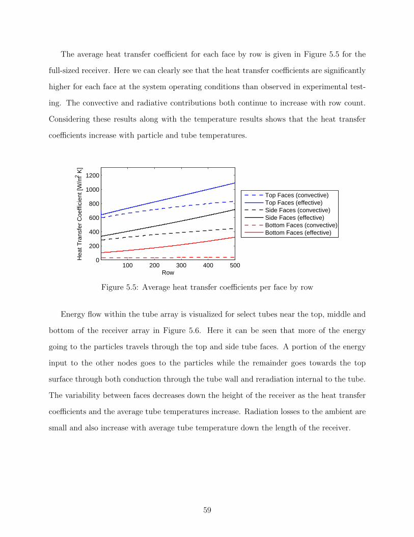
The average heat transfer coefficient for each face by row is given in Figure 5.5 for the

full-sized receiver. Here we can clearly see that the heat transfer coefficients are significantly

higher for each face at the system operating conditions than observed in experimental test-

ing. The convective and radiative contributions both continue to increase with row count.

Considering these results along with the temperature results shows that the heat transfer

coefficients increase with particle and tube temperatures.

100 200 300 400 5000

200

400

600

800

1000

1200

Hea

t Tra

nsfe

r C

oeffi

cien

t [W

/m2 K

]

Row

Top Faces (convective)Top Faces (effective)Side Faces (convective)Side Faces (effective)Bottom Faces (convective)Bottom Faces (effective)

Figure 5.5: Average heat transfer coefficients per face by row

Energy flow within the tube array is visualized for select tubes near the top, middle and

bottom of the receiver array in Figure 5.6. Here it can be seen that more of the energy

going to the particles travels through the top and side tube faces. A portion of the energy

input to the other nodes goes to the particles while the remainder goes towards the top

surface through both conduction through the tube wall and reradiation internal to the tube.

The variability between faces decreases down the height of the receiver as the heat transfer

coefficients and the average tube temperatures increase. Radiation losses to the ambient are

small and also increase with average tube temperature down the length of the receiver.

59

1 2 3 4 5 6 7 8 9 10 11 12 13 14 15

−0.5

0

0.5

1

1.5

Top | Side | Bottom

Hea

t Out

/Sol

ar In

put [

W/W

]

Heat to ParticlesReradiation Losses to AmbientRadiation to Other NodesConduction to Other Nodes

(a) Top Row

1 2 3 4 5 6 7 8 9 10 11 12 13 14 15

−0.5

0

0.5

1

1.5

Top | Side | Bottom

Hea

t Out

/Sol

ar In

put [

W/W

]


(b) Middle Row

1 2 3 4 5 6 7 8 9 10 11 12 13 14 15

−0.5

0

0.5

1

1.5

Top | Side | Bottom

Hea

t Out

/Sol

ar In

put [

W/W

]


(c) Bottom Row

Figure 5.6: Normalized tube energy balances for each tube node

60

5.3 Full Receiver Simulation Discussion

Oscillations in the gas velocity are due to the varying height of the channels. The ver-

tical channels are half the height of the inclined channels within the simulation, therefore,

the cross-sectional area of the gas channel varies and the gas velocity alters to maintain a

constant mass flow rate. This model does not include any recirculation that may occur in a

functional 3D receiver. The cross-sectional area, and therefore gas velocity, are also affected

by changes in the particle flow. Decreasing the depth or solids volume fraction also increases

the effective gas channel area and forces the gas to slow down. The gas velocity, therefore,

varies proportionately with the particle flow depth and solids volume fraction. This effect

is more noticeable in the vertical channels where the changes are more substantial and the

channel is narrower.

The average gas velocity increases with temperature due to expansion. Drag between

this accelerating air and the particles then causes the average particle velocity to increase.

Drag forces remain small relative to the other forces, however, so this increase is slight. As

the average particle velocity increases it also causes the observed decreases in the average

flow depth across the top surface and solids volume fraction within the vertical channels.

The observed convective heat transfer coefficients for the top and side faces are signifi-

cantly higher primarily due to the increased bulk conductivity and thermal diffusivity of the

particles at elevated temperatures. The bottom face convective HTC increases slightly due

to increases in the gas phase conductivity and gas phase velocity that accompany tempera-

ture increases. Additionally, the radiative contribution is much greater due to the increased

temperatures of the interacting surfaces. Continued heating down the length of the receiver

continues to increase both the convective and radiative heat transfer due to further increased

temperatures. These increases in the effective heat transfer coefficients cause the particle

temperatures to approach the tube temperatures and also contribute to a decrease in the

temperature distribution for each tube. Improved tube wall conductivity and increased

reradiation on the solar side of the tube at higher temperatures also contribute to lower

61

tube temperature discrepancies as heat can flow more easily between nodes and over smaller

temperature differences.

Despite the increase in the effective HTC for all faces, the HTC for the top face remains

1.5 times higher than for the side face and 3 times higher than for the bottom face. This

causes the net flow of heat from the bottom of each tube towards the top that is seen in

the energy balances for each node. The amount of heat migrating between nodes decreases

down the height of the receiver due to the increased effective heat transfer coefficients to the

particles.

62

CHAPTER 6

SUMMARY & CONCLUSIONS

This research sought to more fully understand the heat transfer characteristics of the

granular flow within NREL’s Near-Blackbody Enclosed Particle Receiver, a concentrated

solar power concept using hexagonal solar receiver tubes and solid particles as both the

heat transfer fluid and the energy storage medium. This was done through both direct

experimental measurement of the heat transfer coefficients from each face of a single tube

and through the development of a simplified one-dimensional model.

Through low-temperature experimentation, it was discovered that the heat transfer coef-

ficients are overall quite low for the desired application as shown in Table 6.1. In particular,

the bottom face heat transfer coefficient is less than 30 W/m2-K. Visualization of the parti-

cle flow showed that heat transfer coefficients correlate with particle contact. The top face

has particle contact along the full length of the face and the highest HTC, the side face

has intermittent and varied particle contact and a moderate HTC while the bottom face

has little to no particle contact and a low HTC. Studies were also conducted to examine the

average HTC for each of an array of 10 simulated absorber tubes and showed that the erratic

nature of the particle flow can lead to a wide spread in values. Finally, studies also showed

that increases in mass flow rate lead to overall increases in average heat transfer coefficients,

and decreasing the particle diameter showed improved HTC values but at the expense of

decreased maximum flow rates.

Table 6.1: Experimentally determined average heat transfer coefficients for each face atmaximum particle flow conditions using 300 µm particles at 25°C

Tube Face Average Effective Heat Transfer CoefficientTop Face 303 W/m2-KSide Face 156 W/m2-K

Bottom Face 23 W/m2-K

63

In order to more fully understand these results, a model was developed using MATLAB

to simulate heat transfer within the NBB design. Each face of the receiver was described

by a unique heat transfer correlation. The top face was treated as an inclined plate with

sufficient particle contact. For the side face, a correlation for plug flow through a vertical

channel was modified by increasing the “effective” film thickness at the walls to account for

the flow separation observed in experiments. The bottom face was modeled as a thin channel

of air between the bottom tube surface and the upper surface of the granular flow. Entry

length effects are significant over the short length of the face and were accounted for. The

parameters needed for these correlations were calculated using a 1D channel model of the

granular flow. Additionally, the solar side of the tube was included by assuming a constant

input flux to each face and using 3D view factors to capture reradiation effects between tube

nodes and to the ambient. The system was solved by incorporating an energy balance on

the tubes, a mass balance on the gas phase and mass, momentum and energy equations for

the particle flow.

Comparison with the experimental results for the 300 µm particle batch showed good

agreement for all faces at maximum flow rates and captured the overall trends with changes

in mass flow rate. The predicted HTC for the top face at the lowest mass flow rate was higher

than that found in the experiments and a dip occurred in the side face HTC experimental

results at the moderate mass flow rate that was not captured by the model. The model

results also predicted the heat transfer results from the 200 µm particle batch for the top

and bottom faces quite well when the simulation was run with 100 µm particles. This shows

that the presence of increased fine particles in this particle batch had significant impact

on the heat transfer characteristics. The side face heat transfer was not well predicted by

the model. This is likely due to the oversimplification of using a constant “effective” film

thickness.

The model developed was expanded to examine a full-sized NBB receiver by increasing

the row count to 500. The results show that the convective and overall effective heat transfer

64

coefficients are much improved at high temperatures as shown in Table 6.2. This is largely

due to increases in thermal diffusivity and conductivity of the particle phase as temperatures

increase. Additionally, radiation becomes a significant contributor and adds nearly 300

W/m2-K to the HTC for each face. These increases in heat transfer also affect the flow

of energy within each tube. Much of the incident solar flux is transferred towards the top

tube surface by conduction and reradiation. The discrepancy between faces decreases as the

overall average tube temperatures and heat transfer coefficients increase, which also leads to

more uniform temperatures for each tube.

Table 6.2: Model predicted average heat transfer coefficients for each face at maximumparticle flow conditions using 300 µm particles at 800°C

Tube Face Average Effective Heat Transfer CoefficientTop Face 1093 W/m2-KSide Face 716 W/m2-K

Bottom Face 323 W/m2-K

6.1 Future Work

The accuracy of the model shows confidence in this modeling technique. However, sig-

nificant shortcomings do exist. Using a constant “effective” film thickness for the side wall

heat transfer appears to be an oversimplification. Finding ways to correlate this value to the

other flow conditions could improve its accuracy. Additionally, the solar side of the model is

greatly simplified and likely not representative. Incorporating the heat transfer models into

a more complex solar model that includes changes along the length of the tube could prove

beneficial. This was beyond the scope of this project, however, and would likely hinder full

receiver simulations.

Confidence in the model could be improved by high temperature validation. Future work

could include expanded experimentation to allow for such a comparison. Additionally, the

bed friction angle and solids volume fraction across the top face could be directly measured.

65

Despite these shortcomings, the model’s dependency upon the physical dimensions and

real parameters of the system offers the possibility of its use in design studies. Varying the

parameters of the model such as the physical tube dimensions, particle properties and tube

properties could shed light on important design improvements. The model could also be

expanded to the system level to allow for system sizing and cycle analysis.

66

REFERENCES CITED

[1] Renewable resource data center. web. URL http://rredc.nrel.gov/tidbits.html.

[2] Manuel Romero and Jose Gonzalez-Aguilar. Solar thermal csp technology. Wiley In-terdisciplinary Reviews: Energy and Environment, 3(1):42–59, 2014. ISSN 2041-840X.doi: 10.1002/wene.79. URL http://dx.doi.org/10.1002/wene.79.

[3] Craig S. Turchi, Zhiwen Ma, Ty Neises, and Michael Wagner. Thermodynamic Study ofAdvanced Supercritical Carbon Dioxide Power Cycles for High Performance Concentrat-ing Solar Power Systems. In Proceedings of ASME 2012 6th International Conferenceon Energy Sustainability, 2012. doi: 10.1115/ES2012-91179.

[4] Paul Denholm and Marissa Hummon. Simulating the value of concentrating solar powerwith thermal energy storage in a production cost model. Technical Report NREL/TP-6A20-56731, National Renewable Energy Laboratory, November 2012.

[5] Antoni Gil, Marc Medrano, Ingrid Martorell, Ana Lzaro, Pablo Dolado, Beln Zalba,and Luisa F. Cabeza. State of the art on high temperature thermal energy storagefor power generation. part 1concepts, materials and modellization. Renewable and Sus-tainable Energy Reviews, 14(1):31 – 55, 2010. ISSN 1364-0321. doi: http://dx.doi.org/10.1016/j.rser.2009.07.035. URL http://www.sciencedirect.com/science/article/

pii/S1364032109001774.

[6] D. Laing, W. D. Steinmann, P. Veibahn, F. Grater, and C. Bahl. Economic analysisand life cycle assessment of concrete thermal energy storage for parabolic trough powerplants. Journal of Solar Energy Engineering, 132(4), October 2010.

[7] Doerte Laing, Carsten Bahl, Thomas Bauer, Dorothea Lehmann, and Wolf-Dieter Stein-mann. Thermal energy storage for direct steam generation. Solar Energy, 85(4):627 –633, 2011. ISSN 0038-092X. doi: http://dx.doi.org/10.1016/j.solener.2010.08.015. URLhttp://www.sciencedirect.com/science/article/pii/S0038092X10002835. So-larPACES 2009.

[8] Zhiwen Ma, Greg C. Glatzmaier, and Mark Mehos. General development of solid par-ticle thermal energy storage for concentrating solar power plants that use fluidized bedtechnology. In Proceedings of ASME 2013 7th International Conference on Energy Sus-tainability & 11th Fuel Cell Science, Engineering and Technology Conference, 2013.

67

http://rredc.nrel.gov/tidbits.html

http://dx.doi.org/10.1002/wene.79

http://www.sciencedirect.com/science/article/pii/S1364032109001774


http://www.sciencedirect.com/science/article/pii/S0038092X10002835

[9] Zhiwen Ma, Greg Glatzmaier, and Mark Mehos. Fluidized Bed Technology for Con-centrating Solar Power With Thermal Energy Storage. Journal of Solar EnergyEngineering-Transactions of the ASME, 136(3), AUG 2014. ISSN 0199-6231. doi:{10.1115/1.4027262}.

[10] J. Martin and J. Vitko. Ascuas: A solar central receiver utilizing a solid thermal carrier.Technical Report SAND82-8203, Sandia National Laboratories, 1982.

[11] P. K. Falcone, J. E. Noring, and J. M. Hruby. Assessment of a solid particle receiverfor a high temperature solar central receiver system. Technical Report SAND85-8208,Sandia National Laboratories, 1985.

[12] J. M. Hruby. A technical feasibility study of a solid particle solar central receiverfor high temperature applications. Technical Report SAND86-8211, Sandia NationalLaboratories, 1986.

[13] J. Hruby, R. Steeper, G. Evans, and C. Crowe. An experimental and numerical studyof flow and convective heat transfer in a freely falling curtain of particles. Journal ofFluids Engineering, 110(2), 1988. doi: 10.1115/1.3243531.

[14] Nathan P. Siegel, Clifford K. Ho, Siri S. Khalsa, and Gregory J. Kolb. Development andevaluation of a prototype solid particle receiver: On-sun testing and model validation.Journal of Solar Energy Engineering, 132(2), 2010. doi: 10.1115/1.4001146.

[15] Marc Roger, Lars Amsbeck, Birgit Gobereit, and Reiner Buck. Face-down solid particlereceiver using recirculation. Journal of Solar Energy Engineering, 133, August 2011.

[16] Gang Xiao, Kaikai Guo, Zhongyang Luo, Mingjiang Ni, Yanmei Zhang, and ChengWang. Simulation and experimental study on a spiral solid particle solar receiver. Ap-plied Energy, 113(0):178 – 188, 2014. ISSN 0306-2619. doi: http://dx.doi.org/10.1016/j.apenergy.2013.06.045. URL http://www.sciencedirect.com/science/article/pii/

S0306261913005527.

[17] M. J. Rightley, L. K. Matthews, and G. P. Mulholland. Experimental characterizationof the heat transfer in a free-falling-particle receiver. Solar Energy, 48(6):363–374, 1992.

[18] Janna Martinek and Zhiwen Ma. Granular Flow and Heat Transfer Study in aNear-Blackbody Enclosed Particle Receiver. In ASME 2014 8th International Con-ference on Energy Sustainability collocated with the ASME 2014 12th InternationalConference on Fuel Cell Science, Engineering and Technology, volume 1, 2014. doi:10.1115/ES2014-6393.

[19] Zhiwen Ma. Methods and systems for concentrated solar power, 2013.

68



[20] JC Chen, JR Grace, and MR Golriz. Heat transfer in fluidized beds: design methods.Powder Technology, 150(2):123–132, FEB 16 2005. ISSN 0032-5910. doi: {10.1016/j.powtec.2004.11.035}.

[21] VA Borodulya, YS Teplitsky, II Markevich, AF Hassan, and TP Yeryomenko. Heat-transfer between a surface and a fluidized-bed-considerations of pressure and tempera-ture. International Journal of Heat and Mass Transfer, 34(1):47–53, JAN 1991. ISSN0017-9310. doi: {10.1016/0017-9310(91)90171-A}.

[22] H A Vreedenberg. Heat transfer between a fluidized bed and a vertical tube. Chemicalengineering science, 11(4):274 – &, 1960.

[23] H A Vreedenberg. Heat transfer between a fluidized bed and a horizontal tube. Chemicalengineering science, 9(1):52 – 60, 1958.

[24] H. S. Mickley and D. F. Fairbanks. Mechanism of heat transfer to fluidized beds.AIChE Journal, 1(3):374–384, 1955. ISSN 1547-5905. doi: 10.1002/aic.690010317.URL http://dx.doi.org/10.1002/aic.690010317.

[25] Hiromi Takeuchi. Particles flow pattern and local heat transfer around tube in mov-ing bed. AIChE Journal, 42(6):1621–1626, 1996. ISSN 1547-5905. doi: 10.1002/aic.690420613. URL http://dx.doi.org/10.1002/aic.690420613.

[26] J. Niegsch, D. Kneke, and P.-M. Weinspach. Heat transfer and flow of bulk solids in amoving bed. Chemical Engineering and Processing: Process Intensification, 33(2):73 –89, 1994. ISSN 0255-2701. doi: http://dx.doi.org/10.1016/0255-2701(94)85006-2. URLhttp://www.sciencedirect.com/science/article/pii/0255270194850062.

[27] Hany Al-Ansary, Abdelrahman El-Leathy, Zeyad Al-Suhaibani, Sheldon Jeter, DennisSadowski, Abdulaziz Alrished, and Matthew Golob. Experimental study of a sand-airheat exchanger for use with a high-temperature solar gas turbine system. Journal ofSolar Energy Engineering, 134(4), October 2012.

[28] W.N. Sullivan and R.H. Sabersky. Heat transfer to flowing granular media. InternationalJournal of Heat and Mass Transfer, 18(1):97 – 107, 1975. ISSN 0017-9310. doi: http://dx.doi.org/10.1016/0017-9310(75)90012-5. URL http://www.sciencedirect.com/

science/article/pii/0017931075900125.

[29] JK Spelt, CE Brennen, and RH Sabersky. Heat-transfer to flowing granular material.International Journal of Heat and Mass Transfer, 25(6):791–796, 1982. ISSN 0017-9310.doi: {10.1016/0017-9310(82)90091-6}.

69

http://dx.doi.org/10.1002/aic.690010317

http://dx.doi.org/10.1002/aic.690420613

http://www.sciencedirect.com/science/article/pii/0255270194850062



[30] J.S. Patton, R.H. Sabersky, and C.E. Brennen. Convective heat transfer to rapidly flow-ing, granular materials. International Journal of Heat and Mass Transfer, 29(8):1263– 1269, 1986. ISSN 0017-9310. doi: http://dx.doi.org/10.1016/0017-9310(86)90159-6.URL http://www.sciencedirect.com/science/article/pii/0017931086901596.

[31] Matthew Golob, Sheldon Jeter, and Dennis Sadowski. Heat transfer coefficient betweenflat surface and sand. In Proceedings of the ASME 5th International Conference onEnergy Sustainability 2011, PTS A-C, pages 1441–1450, 2012. ISBN 978-0-7918-5468-6.

[32] VVR Natarajan and ML Hunt. Heat transfer in vertical granular flows. ExperimentalHeat Transfer, 10(2):89–107, APR-JUN 1997. ISSN 0891-6152.

[33] VVR Natarajan and ML Hunt. Kinetic theory analysis of heat transfer in granularflows. International Journal of Heat and Mass Transfer, 41(13):1929–1944, JUL 1998.ISSN 0017-9310. doi: {10.1016/S0017-9310(97)00315-3}.

[34] K.S. Rajan, K. Dhasandhan, S.N. Srivastava, and B. Pitchumani. Studies on gas-solid heat transfer during pneumatic conveying. International Journal of Heat andMass Transfer, 51(1112):2801 – 2813, 2008. ISSN 0017-9310. doi: http://dx.doi.org/10.1016/j.ijheatmasstransfer.2007.09.042. URL http://www.sciencedirect.com/

science/article/pii/S0017931007006424.

[35] J. Bandrowski and G. Kaczmarzyk. Gas-to-particle heat transfer in vertical pneumaticconveying of granular materials. Chemical Engineering Science, 33(10):1303 – 1310,1978. ISSN 0009-2509. doi: http://dx.doi.org/10.1016/0009-2509(78)85111-2. URLhttp://www.sciencedirect.com/science/article/pii/0009250978851112.

[36] J Guderian, D Kneke, and P.-M Weinspach. Heat transfer to trickling granular materials.Chemical Engineering and Processing: Process Intensification, 30(3):157 – 174, 1991.ISSN 0255-2701. doi: http://dx.doi.org/10.1016/0255-2701(91)85005-9. URL http:

//www.sciencedirect.com/science/article/pii/0255270191850059.

[37] Yoel Forterre and Olivier Pouliquen. Flows of dense granular media. Fluid Mechanics,40:1–24, January 2008.

[38] GDR Midi. On dense granular flows. The European Physical Journal E, 14(4):341–365,2004. ISSN 1292-8941. doi: 10.1140/epje/i2003-10153-0. URL http://dx.doi.org/

10.1140/epje/i2003-10153-0.

[39] Michel Y. Louge and Stephen C. Keast. On dense granular flows down flat frictional in-clines. Physics of Fluids (1994-present), 13(5):1213–1233, 2001. doi: http://dx.doi.org/10.1063/1.1358870. URL http://scitation.aip.org/content/aip/journal/pof2/

13/5/10.1063/1.1358870.

70







http://dx.doi.org/10.1140/epje/i2003-10153-0

http://dx.doi.org/10.1140/epje/i2003-10153-0

http://scitation.aip.org/content/aip/journal/pof2/13/5/10.1063/1.1358870

http://scitation.aip.org/content/aip/journal/pof2/13/5/10.1063/1.1358870

[40] R. Delannay, M. Louge, P. Richard, N. Taberlet, and A. Valance. Towards a theoreticalpicture of dense granular flows down inclines. Nature Materials, 6:99–108, February2007.

[41] Birte Domnik and Shiva P. Pudasaini. Full two-dimensional rapid chute flows of simpleviscoplastic granular materials with a pressure-dependent dynamic slip-velocity andtheir numerical simulations. Journal of Non-Newtonian Fluid Mechanics, 173:72–86,APR 2012. ISSN 0377-0257. doi: {10.1016/j.jnnfm.2012.03.001}.

[42] Birte Domnik, Shiva P. Pudasaini, Rolf Katzenbach, and Stephen A. Miller. Couplingof full two-dimensional and depth-averaged models for granular flows. Journal of Non-Newtonian Fluid Mechanics, 201:56–68, NOV 2013. ISSN 0377-0257. doi: {10.1016/j.jnnfm.2013.07.005}.

[43] Colin Bailey. Stainless steel thermal properties. URL http://www.mace.

manchester.ac.uk/project/research/structures/strucfire/materialInFire/

Steel/StainlessSteel/thermalProperties.htm.

[44] John R. Howell. A catalog of radiation heat transfer configuration factors. web. URLhttp://www.thermalradiation.net/indexCat.html.

[45] Theodore L. Bergman, Adrienne S. Lavine, Frank P. Incropera, and David P. Dewitt.Fundamentals of heat and Mass Transfer. John Wiley & Sons, 2011.

[46] R. K. Shah and A. L. London. Laminar Flow Forced Convection in Ducts. Advances inHeat Transfer. Academic Press, 1978.

[47] Andrew Oles. Modeling of Solar Particle Receivers for Hydrogen Production and Ther-mochemical Energy Storage. PhD thesis, University of Maryland, 2014.

[48] G Malherbe, J-F Henry, A El Bakali, C Bissieux, and S Fohanno. Measurement of ther-mal conductivity of granular materials over a wide range of temperatures. comparisonwith theoretical models. Journal of Physics: Conference Series, 395(1):012081, 2012.URL http://stacks.iop.org/1742-6596/395/i=1/a=012081.

[49] Clayton Crowe, Martin Sommerfeld, and Yutaka Tsuji. Multiphase Flows with Dropletsand Particles. CRC Press, 1998.

[50] Kevin Albrecht. Multiphase, multi-component, chemically reacting, counter-current,channel flow using a eulerian approach. August 2014.

[51] Ihsan Barin. Thermochemical Data of Pure Substances. Weinheim, 2nd edition, 1993.

71

http://www.mace.manchester.ac.uk/project/research/structures/strucfire/materialInFire/Steel/StainlessSteel/thermalProperties.htm



http://www.thermalradiation.net/indexCat.html

http://stacks.iop.org/1742-6596/395/i=1/a=012081

experimental and numerical analysis of heat transfer in a ... · experimental measurement of the...

Documents