expectation propagation as a solution for digital

Doctoral ThesisPhD in Automatic, Electronics andTelecommunication Engineering

Expectation Propagation as aSolution for DigitalCommunication Systems

Author: Irene Santos VelázquezAdvisors: Juan José Murillo Fuentes

Eva María Arias de Reyna Domínguez

Teoría de la Señal y ComunicacionesEscuela Técnica Superior de IngenieríaUniversidad de Sevilla

Sevilla, 2018

brought to you by COREView metadata, citation and similar papers at core.ac.uk

provided by idUS. Depósito de Investigación Universidad de Sevilla

https://core.ac.uk/display/186617012?utm_source=pdf&utm_medium=banner&utm_campaign=pdf-decoration-v1

Doctoral ThesisPhD in Automatic, Electronics and Telecommunication

Engineering

Expectation Propagation as a Solution for DigitalCommunication Systems

Author:

Irene Santos Velázquez

Advisors:

Juan José Murillo FuentesProfesor Catedrático

Eva María Arias de Reyna DomínguezProfesor Contratado Doctor

Teoría de la Señal y ComunicacionesEscuela Técnica Superior de Ingeniería

Universidad de Sevilla

2018

Tesis Doctoral: Expectation Propagation as a Solution for Digital CommunicationSystems

Autor: Irene Santos VelázquezDirectores: Juan José Murillo Fuentes

Eva María Arias de Reyna Domínguez

El tribunal nombrado para juzgar la Tesis arriba indicada, compuesto por los sigu-ientes doctores:

Presidente:

Vocales:

Secretario:

acuerdan otorgarle la calificación de:

El Secretario del Tribunal

Fecha:

Agradecimientos

Me gustaría comenzar agradeciendo a aquellas personas sin las cuales esta tesisno hubiera sido posible.

Juanjo, creo que no podría haber encontrado un mejor tutor/director de la tesisque tú. Quiero agradecerte la oportunidad que me diste hace cuatro años parainiciarme en el mundo de la investigación contigo. Sin tus consejos, enseñanza ydedicación no hubiera podido sacar adelante este trabajo.Eva, tenerte como co-directora ha sido un privilegio y una pieza fundamental

para desarrollar esta tesis. Gracias por tu tiempo y minuciosidad. Han sido clavepara que la tesis sea lo más clara y amigable posible.

No pueden faltar tampoco mis responsables de estancia, Petar y Pablo. Graciaspor enseñarme nuevas líneas de investigación y por toda vuestra ayuda durante miestancia.

También quiero agradecer a todos mis compañeros de Departamento, en especiala los fieles de la hora del desayuno: Rafa, Irene, Uxi y Javier (aunque sólo desayuneslos viernes). Por supuesto, también a todos mis compis de sala, porque me estánhaciendo una experta en música y hacen mi día a día mucho más divertido.

Y no puedo terminar sin agradecer a mis padres, mi hermano y Javi. Porque sinvuestro apoyo incondicional sé que no lo hubiera conseguido.

I

Abstract

In the context of digital communications, a digital receiver is required to providean estimation of the transmitted symbols. Nowadays channel decoders highlybenefit from soft (probabilistic) estimates for each transmitted symbol rather thanfrom hard decisions. For this reason, digital receivers must be designed to providethe probability that each possible symbol was transmitted based on the receivedcorrupted signal. Since exact inference might be unfeasible in terms of complexityfor high-order scenarios, it is necessary to resort to approximate inference, suchas the linear minimum mean square error (LMMSE) criterion. The LMMSEapproximates the discrete prior information of the transmitted symbols with aGaussian distribution, which causes a degradation in its performance. In this thesis,an alternative approximate statistical technique is applied to the design of a digitalprobabilistic receiver in digital communications. Specifically, the expectationpropagation (EP) algorithm is investigated to find the Gaussian posterior probabilitydensity function (pdf) that minimizes the Kullback-Leibler (KL) divergence withrespect to the true posterior pdf.

Two different communication system scenarios are studied: a single-input single-output (SISO) digital communication system with memory channel and a multiple-input multiple-output (MIMO) system with memoryless channel. In the SISOscenario, three different designs of a soft standalone and turbo equalizer basedon the EP algorithm are developed: the block or batch approach, the filter-typeversion that emulates the Wiener filter behavior and the smoothing equalizer whichproceeds similarly to a Kalman smoother. Finally, the block EP implementationis also adapted to MIMO scenarios with feedback from the decoder. In bothscenarios, the EP is applied iteratively, including a damping mechanism and acontrol to avoid negative values of variances, which would lead to instabilities(specially for high-order constellations). Experimental results included through

III

IV Abstract

the thesis show that the EP algorithm applied to communication systems greatlyimproves the performance of previous approaches found in the literature with acomplexity slightly increased but still proportional to that of the LMMSE. Theseresults also show the robustness of the algorithm even for high-order modulations,large memory channels and high number of antennas.

Major contributions of this dissertation have been published in four journal (oneof them is still under review) and two conference papers. One more paper will besubmitted to a journal soon. All these papers are listed below:

• Irene Santos, Juan José Murillo-Fuentes, Rafael Boloix-Tortosa, Eva Ariasde Reyna and Pablo M. Olmos, "Expectation Propagation as Turbo Equalizerin ISI Channels," IEEE Transactions on Communications, vol. 65, no.1, pp.360-370, Jan 2017.

• Irene Santos, Juan José Murillo-Fuentes, Eva Arias de Reyna and Pablo M.Olmos, "Turbo EP-based Equalization: a Filter-Type Implementation," IEEETransactions on Communications, Sep 2017, Accepted. [Online] Available:https://ieeexplore.ieee.org/document/8353388/

• Irene Santos, Juan José Murillo-Fuentes, Eva Arias-de-Reyna and Pablo M.Olmos, "Probabilistic Equalization With a Smoothing Expectation Propaga-tion Approach," IEEE Transactions on Wireless Communications, vol. 16,no. 5, pp. 2950-2962, May 2017.

• Irene Santos, Juan José Murillo-Fuentes and Eva Arias-de-Reyna, "Equal-ization with Expectation Propagation at Smoothing Level," To be submitted.[Online] Available: https://arxiv.org/abs/1809.00806

• Irene Santos and Juan José Murillo-Fuentes, "EP-based turbo detection forMIMO receivers and large-scale systems," IEEE Transactions on VehicularTechnology, May 2018, Under review. [Online] Available:https://arxiv.org/abs/1805.05065

• Irene Santos, Juan José Murillo-Fuentes, and Pablo M. Olmos, "Blockexpectation propagation equalization for ISI channels," 23rd European SignalProcessing Conference (EUSIPCO 2015), Nice, 2015, pp. 379-383.

• Irene Santos, and Juan José Murillo-Fuentes, "Improved probabilistic EP-based receiver for MIMO systems and high-order modulations," XXXIIISimposium Nacional de la Unión Científica Internacional de Radio (URSI2018), Granada, 2018.

Resumen

En el ámbito de las comunicaciones digitales, es necesario un receptor digital queproporcione una estimación de los símbolos transmitidos. Los decodificadores decanal actuales se benefician enormemente de estimaciones suaves (probabilísticas)de cada símbolo transmitido, en vez de estimaciones duras. Por este motivo, losreceptores digitales deben diseñarse para proporcionar la probabilidad de cadaposible símbolo que fue transmitido en base a la señal recibida y corrupta. Dadoque la inferencia exacta puede no ser posible en términos de complejidad paraescenarios de alto orden, es necesario recurrir a inferencia aproximada, como porejemplo el criterio de linear minimum-mean-square-error (LMMSE). El LMMSEaproxima la información a priori discreta de los símbolos transmitidos con unadistribución Gaussiana, lo cual provoca una degradación en su resultado. Enesta tesis, se aplica una técnica alternativa de inferencia estadística para diseñarun receptor digital probabilístico de comunicaciones digitales. En concreto, seinvestiga el algoritmo expectation propagation (EP) con el objetivo de encontrar lafunción densidad de probabilidad (pdf) a posteriori Gaussiana que minimiza ladivergencia de Kullback-Leibler (KL) con respecto a la pdf a posteriori verdadera.

Se estudian dos escenarios de comunicaciones digitales diferentes: un sistema decomunicaciones single-input single-output (SISO) con canales con memoria y unsistema multiple-input multiple-output (MIMO) con canales sin memoria. Para elescenario SISO se proponen tres diseños diferentes para un igualador probabilístico,tanto simple como turbo, que está basado en el algoritmo EP: una versión bloque,una versión filtrada que emula el comportamiento de un filtro Wiener y una versiónsmoothing que funciona de forma similar a un Kalman smoother. Finalmente, laimplementación del EP en bloque se adapta también para escenarios MIMO conrealimentación desde el decodificador. En ambos escenarios, el EP se aplica deforma iterativa, incluyendo un mecanismo de damping y un control para evitar

V

VI Resumen

valores de varianzas negativas, que darían lugar a inestabilidades (especialmente, enconstelaciones de alto orden). Los resultados experimentales que se incluyen en latesis muestran que, cuando el algoritmo EP se aplica a sistemas de comunicaciones,se mejora notablemente el resultado de otras propuestas anteriores que existen enla literatura, con un pequeño incremento de la complejidad que es proporcional a lacarga del LMMSE. Estos resultados también demuestran la robustez del algoritmoincluso para modulaciones de alto orden, canales con bastante memoria y un grannúmero de antenas.

Las principales contribuciones de esta tesis se han publicado en cuatro artículosde revista (uno de ellos todavía bajo revisión) y dos artículos de conferencia. Otroartículo adicional se encuentra en preparación y se enviaría próximamente a unarevista. Estos se citan a continuación:

• Irene Santos, Juan José Murillo-Fuentes, Rafael Boloix-Tortosa, Eva Ariasde Reyna and Pablo M. Olmos, "Expectation Propagation as Turbo Equalizerin ISI Channels," IEEE Transactions on Communications, vol. 65, no.1, pp.360-370, Jan 2017.

• Irene Santos, Juan José Murillo-Fuentes, Eva Arias de Reyna and PabloM. Olmos, "Turbo EP-based Equalization: a Filter-Type Implementation,"IEEE Transactions on Communications, Sep 2017, Aceptado. [Online]Disponible: https://ieeexplore.ieee.org/document/8353388/

• Irene Santos, Juan José Murillo-Fuentes, Eva Arias-de-Reyna and Pablo M.Olmos, "Probabilistic Equalization With a Smoothing Expectation Propaga-tion Approach," IEEE Transactions on Wireless Communications, vol. 16,no. 5, pp. 2950-2962, May 2017.

• Irene Santos, Juan José Murillo-Fuentes and Eva Arias-de-Reyna, "Equal-ization with Expectation Propagation at Smoothing Level," En preparación.[Online] Disponible: https://arxiv.org/abs/1809.00806

• Irene Santos and Juan José Murillo-Fuentes, "EP-based turbo detection forMIMO receivers and large-scale systems," IEEE Transactions on VehicularTechnology, May 2018, En revisión. [Online] Disponible:https://arxiv.org/abs/1805.05065

• Irene Santos, Juan José Murillo-Fuentes, and Pablo M. Olmos, "Blockexpectation propagation equalization for ISI channels," 23rd European SignalProcessing Conference (EUSIPCO 2015), Nice, 2015, pp. 379-383.

• Irene Santos, and Juan José Murillo-Fuentes, "Improved probabilistic EP-based receiver for MIMO systems and high-order modulations," XXXIII

Resumen VII

Simposium Nacional de la Unión Científica Internacional de Radio (URSI2018), Granada, 2018.

Contents

Abstract IIIResumen VNotation XIII

1 Introduction 11.1 Motivation and objectives 11.2 Thesis overview 4

2 State of the art 72.1 Standalone and turbo equalization 7

2.1.1 Optimal equalization 72.1.2 Approximations to the BCJR 82.1.3 The LMMSE as equalizer 92.1.4 Message-passing equalization 102.1.5 EP-based equalization 10

2.2 MIMO detection 11

3 Standalone equalization 153.1 Problem to solve 15

3.1.1 System model 163.2 EP-based equalizers 17

3.2.1 Block Expectation Propagation (BEP) 223.2.2 Filter expectation propagation (FEP) 243.2.3 Kalman smoothing expectation propagation (KSEP) 25

3.3 Experimental results 293.4 Conclusions 30

IX

X Contents

4 Turbo equalization 334.1 Problem to solve 33

4.1.1 System model 334.2 EP-based turbo equalizers 35

4.2.1 Single EP turbo equalization 354.2.2 Double EP turbo equalization 354.2.3 Implementation of the proposed generic EP-based equalizer 37

4.3 Turbo block expectation propagation (T-BEP) 394.4 Turbo filter expectation propagation (T-FEP) 404.5 Turbo Kalman smoothing expectation propagation (T-KSEP) approach 414.6 Experimental results 42

4.6.1 Comparison of all the proposed schemes for turbo EP-basedequalizers 45

4.6.2 Comparison with other EP-based approaches in the literature 464.7 Conclusions 47

5 Application to turbo MIMO detection 495.1 Problem to solve 49

5.1.1 System model 495.2 EP-based turbo detectors 51

5.2.1 Turbo block expectation propagation (T-BEP) for MIMO 525.2.2 Related approaches 53

5.3 Experimental results 555.4 Conclusions 56

6 Conclusions 616.1 Summary of results 626.2 Future lines 64

Appendix A Paper I 67

Appendix B Paper II 79

Appendix C Paper III 93

Appendix D Paper IV 107

Appendix E Conference publications 113E.1 Paper I 113

Contents XI

E.2 Paper II 119

List of Figures 125List of Tables 127Bibliography 129Glossary 137

Notation

R(·) real partI(·) imaginary partu scalaru column vectorU matrixui or u(i) i-th element of the vector uui: j column vector with the entries of u, in the range [i, j] in

increasing order if i< j, or in the range [ j,i] in decreasingorder otherwise

u\i vector u without the i-th componentU\i submatrix obtained by removing from U the i-th row and

columndiag(u) returns a diagonal matrix with diagonal given by uCN(u : m,C) normal distribution of a random proper complex vector

u with mean m and covariance matrix C(·)H hermitian(·)∗ complex conjugate(·)−1 inverse∝ proportional to∼ distributed according toI identity matrixI indicator functionO(·) computational cost in operationsProjG[·] projection of the distribution given as an argument into

the family of Gaussians

XIII

XIV Notation

δ (·) delta functionE(·) expected value of the variable in (·)

K length of the transmitted bit sequenceV length of the coded bit vectorN length of the transmitted frameR= K/V code rateM modulation/constellation sizeQ = log2(M) required bits for each symbol of the constellationA set of symbols of the constellationL length (number of taps) of the channel state information

(CSI)L= L−1 memory of the CSINt number of transmit antennasNr number of receive antennasa = [a1,...,aK]> information bit sequence where ai ∈ {0,1}a = [a1,...,aK]> estimated information bit sequenceb = [b1,...,bV]> coded bit vector where bt ∈ {0,1}c = [c1,...,cV]> coded bit vector after permuting the bits with an inter-

leaver where ct ∈ {0,1}c = [c1,...,cN]> permuted coded bit vector after partitioning it into N

blocks where ck = [ck,1, · · · ,ck,Q]u modulated (or transmitted) symbols where uk ∈A

u estimated transmitted symbolsh = [h1,...,hL]> CSIhL:1 = [hL,...,h1]

> flipped CSIy received signalσ2

w noise variancew additive white Gaussian noise (AWGN) where

wk ∼ CN(wk : 0,σ2

w)

H channel matrixEs the mean transmitted symbol energyEb the energy per bitS number of EP iterations` index of the EP iteration, ` ∈ [1,S]β smoothing parameter used in the EP algorithmε minimum allowed variance used in the EP algorithmT number of turbo iterationst index of the turbo iteration, t ∈ [0,T ]

Notation XV

W length of the window in filtered or windowed algorithmsp(u|y) true posterior pdfp(uk|y) k-th marginal of the true posterior pdfq(u) approximated posterior pdfq(uk) k-th marginal of the full approximated posterior pdfpE(uk) true extrinsic pdf for the k-th symbolqE(uk) approximated extrinsic pdf for the k-th symbolpD(·) true probabilistic information returned by the channel

decoderL(·) posterior log-likelihood ratio (LLR) at the input of the

decoderLE(·) extrinsic LLR at the input of the decoderLD(·) extrinsic LLR at the output of the decoderq[`](uk) k-th marginal of the full approximated posterior pdf at

`-th EP iteration, q[`](uk)∼ CN(

uk : µ[`]k ,s2[`]

k

)

q[`]E (uk) approximated extrinsic pdf at `-th EP iteration for thek-th symbol, q[`]E (uk)∼ CN

(uk : z[`]k ,v2[`]

k

)

p[`](uk) factors of an approximated prior at `-th EP iteration,p[`](uk)∼ CN

(uk : m[`]

k ,η[`]k

)

ϕ j(u) j-th bit associated to the demapping of symbol u

1 Introduction

1.1 Motivation and objectives

Current digital communication systems need to transmit sequences of informationbits over communication channels, providing high-speed data and high-qualityservices. During the propagation process, the digital transmission is corruptedby additive white Gaussian noise (AWGN), intersymbol interference (ISI) andinterference from other users, channels of antennas, among others. All these eventsnegatively affect the received signal. In many scenarios, the above problem can beexpressed as

y = Hu+w, (1.1)

where y, u, H and w are the received and transmitted signals, the channel matrixand the AWGN noise, respectively. Through this thesis, the channel matrix will beperfectly known and the noise will be distributed according to w∼ CN(w : 0,Cw),i.e., a circular complex Gaussian distribution with mean 0 and covariance matrixCw. In (1.1), w accounts for the noise while H models the interference.The goal of a digital receiver is to provide an estimation of the transmitted

sequence of symbols, u, from the received corrupted signal, as shown in Figure 1.1.To further improve the estimation, a forward error correction (FEC) is usuallyintroduced. At the transmitter, the channel encoder includes some redundancy toprotect the data, by means of an error correction code (ECC). At the receiver, thechannel decoder exploits the redundancy to significantly improve the estimation ofthe transmitted sequence, reducing the resulting bit error rate (BER). Furthermore,the estimation provided by the digital receiver can be further refined by feeding itback with the output of the channel decoder, as it is shown with dashed lines in

1

2 Chapter 1. Introduction

Figure 1.1. This exchange of information between the receiver and the channeldecoder is usually referred to as turbo scheme.

ChannelCoder H

Digital RX forcoded symbols

ChannelDecoder

a u

w

y u a

p(u)

Figure 1.1 System model of a digital communication system.

The most straightforward way to estimate the transmitted symbols is by mak-ing hard decisions on the sequence of channel symbols that were transmitted.Nowadays channel decoders highly benefit from soft (probabilistic) estimates foreach transmitted symbol, rather than from hard decisions. For this reason, digitalreceivers must be designed to provide to the channel decoder the probability oftransmitting each possible symbol based on the received corrupted signal, i.e., theposterior probability. One commonly used technique to obtain this probability atthe receiver is based on Bayesian inference.One optimal criterion in Bayesian inference, known as maximum a posteri-

ori (MAP) criterion, finds the estimation of a variable of interest given someobservations by minimizing the probability of error. In the context of digitalcommunications, the variable of interest and the observations are the transmittedand received signals, respectively. To compute the estimation of the transmittedsequence that was most probably transmitted, the MAP algorithm maximizes the aposteriori probabilities (APP) given the received signal, i.e.,

u = argmaxu

p(u|y) (1.2)

where, in case of the linear model of the digital communication system in (1.1),

p(u|y) = p(y|u)p(u)p(y)

∝ CN(y : Hu,Cw) p(u) (1.3)

and the prior information of the transmitted symbols, p(u), follows a discretedistribution1.

An alternative Bayesian estimator is the minimum mean square error (MMSE),that computes an estimation of the transmitted signal by minimizing the mean

1 This prior information is given by the output of the channel decoder. When no feedback is availablefrom the decoder and the transmitted symbols are assumed to be equiprobable, this prior is normallyset to a uniform distribution.

1.1 Motivation and objectives 3

square error (MSE) between the transmitted signal and its estimation or, equiva-lently,

u = E(u|y) =∫

up(u|y)du. (1.4)

The covariance matrix of this estimator can be computed as

Cu|y =∫(u−E(u|y))(u−E(u|y))H p(u|y)du. (1.5)

Both estimators require the computation of the posterior pdf in (1.3), whose close-form analytical expression may not be obtained (except for the simplest typesof probabilistic models, such as Gaussians), or it might be unfeasible in termsof complexity. These two approaches in (1.2) and (1.4)-(1.5), where the exactposterior is employed, are usually referred to as exact inference [4, 31, 26].

When the analytical expression of the posterior cannot be obtained, it is nec-essary to resort to approximation schemes, referred to as approximate inference.One common assumption is that the transmitted and received signals are jointlyGaussian,

[uy

]∼ CN

([uy

]:[

mumy

],

[Cu CuyCyu Cy

]), (1.6)

yielding a Gaussian and tractable posterior pdf whose mean vector and covariancematrix are given by

E(u|y) = mu +CuyC−1y (y−my), (1.7)

Cu|y = Cu−CuyC−1y Cyu. (1.8)

This approximation implies that u ∼ CN(u : mu,Cu). Hence, it follows that theapproximation to the posterior in (1.3) is distributed as

q(u) ∝ CN(y : Hu,Cw)CN(u : mu,Cu)∼ CN(u : u,Cu|y

)(1.9)

and the estimator yields

u = mu +CuHH(HCuHH +Cw

)−1(y−Hmu), (1.10)

Cu|y = Cu−CuHH(HCuHH +Cw

)−1 HCu. (1.11)

This estimation is commonly referred to as linear minimum mean square error(LMMSE).


Asmentioned before, in the context of digital communications, the prior informa-tion of the transmitted symbols follows a discrete distribution. Therefore, assuminga Gaussian prior distribution for these symbols degrades their estimation. The goalof this thesis lies on the design of alternative approximate statistical techniques thatwill be applied for the design of digital probabilistic receivers for communicationsystems to provide a good compromise between performance and computationalcomplexity. Specifically, the expectation propagation (EP) algorithm is investi-gated to find the Gaussian posterior pdf that minimizes the Kullback-Leibler (KL)divergence with respect to the true posterior pdf [33, 32, 53, 4, 59].In this thesis, different novel designs of a probabilistic EP-based receiver are

proposed for both SISO and MIMO scenarios. These receivers greatly outperformthe performance of the LMMSE and previous approaches found in the literature,with a complexity slightly increased but still proportional to the LMMSE one.These novel receivers show a robust behavior regardless of the order of the modu-lation, the length of the channel and the number of antennas. The scope of thisthesis encompasses time domain receivers and linear time invariant (LTI) systems.The proposed EP algorithms are part of the first subsystem of the digital receiverof Figure 1.1. In the SISO scenario, this subsystem is an equalizer while in theMIMO scenario it is a detector.

1.2 Thesis overview

In this thesis, we deal with two different scenarios of a communication system:a SISO system with memory channels and a MIMO system with memorylesschannels. The literature about digital receivers employed in both scenarios isinvestigated in Chapter 2. The main part of this thesis is focused on the SISOscenario where several EP-based equalizers are proposed. In Chapter 3 we focuson the standalone equalizer to later extended it for turbo equalization in Chapter 4.Specifically, three different designs of a soft equalizer based on the EP algorithmare developed: the block or batch approach, the filter-type version that emulatesthe Wiener filter behavior and the smoothing equalizer that proceeds similarly to aKalman filter. These designs were developed as part of a collection of publishedscientific articles listed below, including the Appendix where they can be found inthis thesis:

• AppendixA: Irene Santos, Juan JoséMurillo-Fuentes, Rafael Boloix-Tortosa,Eva Arias de Reyna and Pablo M. Olmos, "Expectation Propagation as TurboEqualizer in ISI Channels," IEEE Transactions on Communications, vol. 65,no.1, pp. 360-370, Jan 2017. [50]

1.2 Thesis overview 5

In this paper, the block/batch approach for the EP equalizer is developed.Since the computational complexity of the algorithm is dominated by theinversion of a matrix, its structure is exploited to reduce this computation.Specifically, its complexity is O(SN2L), where N is the length of the trans-mitted frame, L the length of the channel and S is the number of iterationsof the EP algorithm.

• Appendix B: Irene Santos, Juan José Murillo-Fuentes, Eva Arias de Reynaand Pablo M. Olmos, "Turbo EP-based Equalization: a Filter-Type Imple-mentation," IEEE Transactions on Communications, Sep 2017, Accepted.[Online] Available: https://ieeexplore.ieee.org/document/8353388/ [48]

In this paper, the previous block proposal is reviewed and optimized for turboequalization. A Wiener filter-type EP-based equalizer is also developed,whose complexity is dominated by the inversion of a matrix with size givenby the length of the window, W, i.e., O(SNW2). This solution reduces thecomputational complexity compared to the block design at the cost of adegradation in performance. Finally, the EP parameters are revised to reducethe number of EP iterations in a turbo scheme.

• Appendix C: Irene Santos, Juan José Murillo-Fuentes, Eva Arias-de-Reynaand Pablo M. Olmos, "Probabilistic Equalization With a Smoothing Expec-tation Propagation Approach," IEEE Transactions on Wireless Communica-tions, vol. 16, no. 5, pp. 2950-2962, May 2017. [49]

In this paper, a smoothing Kalman implementation of the EP-based equalizeris proposed. Its computational complexity is dominated by the inversion ofa matrix whose size is given by the length of the window used. It achievesthe same performance as the block design with lower complexity given byO(SNL3).

These three different designs have one characteristic in common: they use theEP algorithm to approximate with Gaussians the posterior pdf at the output ofthe equalizer. This strategy is different to what can be found in the literature[58, 24, 66] where the EP is used to pass the discrete information from the channeldecoder to the LMMSE equalizer, not improving the solution of a standaloneequalizer without decoder. To take the advantages of both approaches, in Chapter 4they are combined into a novel double EP-based approach. Chapter 5 focuseson the MIMO scenario and develops a block EP-based turbo receiver followingthe guidelines of our previous works on turbo equalization. This novel receiveroutperforms previous approaches found in the literature [5, 8, 54]. It has also beensubmitted to a journal, where it is currently under review:


• Appendix D: Irene Santos and Juan José Murillo-Fuentes, "EP-based turbodetection for MIMO receivers and large-scale systems," IEEE Transac-tions on Vehicular Technology, May 2018, Submitted. [Online] Available:https://arxiv.org/abs/1805.05065 [46]In this paper, the EP algorithm is applied to MIMO systems in a block formand a turbo scheme. Based on our previous articles in equalization, weemployed the revised EP parameters to reduce the computational complexityof the algorithm.

Conclusions and future lines of research are included in Chapter 6. Finally, Ap-pendix A to Appendix D contain the main scientific contributions of this disserta-tion [50, 48, 49, 46] and Appendix E includes some related conference papers.

2 State of the art

2.1 Standalone and turbo equalization

Soft equalizers provide a posterior pdf of the transmitted symbols given a set ofobservations, from which nowadays channel decoders highly benefit. In addition,this soft information can be further refined by feeding the output of the channeldecoder back to the probabilistic equalizer. This new information is consideredby the equalizer as an updated prior information about the transmitted symbols.This exchange of information between the equalizer and the channel decoder isknown as turbo equalization. If no turbo equalization is performed, we refer to theequalization step as standalone equalization.

2.1.1 Optimal equalization

Optimal equalization methods must minimize the symbol error rate (SER), whichcan be based on MAP estimations. One efficient MAP method is the BCJRalgorithm [1], which requires perfect knowledge of the channel state information(CSI). The BCJR works on a trellis representation defined by states and computesthe transition probability between consecutive trellis states in three different steps[29]. First, the forward filtering step computes the probability from a state to thenext one, given a new observation through the trellis. Second, a similar filteringstep is performed backwards. Finally, a smoothing step computes the APP for eachsymbol from the transition probabilities of both filtering procedures. However,the BCJR becomes unfeasible for multilevel modulations and/or few taps of thechannel since its computational complexity is proportional to the number of trellisstates, ML, where M is the constellation size and L the number of taps of the channel.

7

8 Chapter 2. State of the art

2.1.2 Approximations to the BCJR

A variety of solutions can be found in the literature to reduce the complexity of thetrellis diagram used by the BCJR algorithm, at the expense of performance loss[10, 19, 18, 63, 55]. Instead of considering the full trellis, they perform a simplifiedtrellis search with only Me� ML states. They can be divided into two differentfamilies. The first one is based on truncating the number of trellis states by keepingonly the states with highest forward (or backward) metric or whose forward (orbackward) metric is above a predefined threshold, which is the case of the M-BCJRand T-BCJR algorithms [19], respectively. Basically, they perform a reducedsearch on the original full trellis. On the other hand, the second family consistson truncating the effective length of the CSI by cancelling the last channel taps(retaining just L′ < L taps) and therefore reducing the number of states to Me = ML

′ .In contrast to the first family, this one performs a full search on a reduced-statetrellis. This is the case of the channel shortening (CS) approaches, such as [43],and the reduced-state BCJR (RS-BCJR) algorithm [55], originally inspired by thereduced-state sequence detection (RSSD) [16, 15, 9]. To enhance the results ofboth trends, a posterior approach mixes both families into the M*-BCJR algorithm[10], which keeps the states with highest forward metric, as the M-BCJR does, butinstead of deleting the remaining states, they are merged into the surviving states,similarly to the RS-BCJR strategy.The previous approaches have an important limitation: the surviving paths

cannot be computed by the forward and backward procedures independently, sincethese paths generally do not match in both procedures. To overcome this situation,they give a predominant role to the forward recursion, so that the backward stagejust follows the subset of paths previously selected in the forward stage. For thisreason, they might not succeed when equalizing maximum-phase channels. On thecontrary, if they give a predominant role to the backward recursion, instead of theforward one, they do not succeed with minimum-phase channels [18]. To solve theprevious limitation, a different state selection criterion is proposed in [63]. Insteadof selecting the states with largest metric as the M-BCJR algorithm, they keep thestates with largest values of its marginal APP and repeat the forward/backward pro-cedure allowing different sets of surviving states at each iteration. The performancedependence of these approaches with the type of channel is deeply studied in [18].The authors propose equalizing according to the minimum, maximum or mixedphase nature of the channel, resorting to the forward-trellis (FT), backward-trellis(BT) or a mixture of them named doubled-trellis (DT), respectively. The authorsalso mention that all the approximated BCJR methods select the most promisingpaths while performing the reduced search over the trellis, i.e., they ignore somepaths in the trellis. For this reason, the estimation of their decisions are normally

2.1 Standalone and turbo equalization 9

considered more reliable than they really are. To mitigate this overestimation, theyintroduce an output saturation to their previous proposals [18].All these approximated BCJR approaches suffer from two major drawbacks.

Firstly, they are usually designed and tested for just some specific channels and theparameters are selected according to those channels and the simulated scenario.In general, no information is given about how to tune these parameters for otherchannels. Secondly, they are intractable for large trellises since their performancedegrades if the number of surviving states, Me, does not grow accordingly with thetotal number of states, i.e, if the ratio ML−1/Me is not kept constant at a relativelyhigh value. To the best of our knowledge, this issue has not been studied andthe value for this ratio to ensure an accurate enough performance remains asan open question. For these reasons, these approximated BCJR approaches areonly interesting for a moderate number of states. For large number of states, it ispreferable to envisage filter-based equalizers of the MMSE type [2] or message-passing approaches [12, 11, 21, 24, 58, 66].

2.1.3 The LMMSE as equalizer

The LMMSE algorithm is commonly used for soft equalization since it provides asuboptimal but low-cost and robust estimation even for multidimensional modu-lations. It is derived for a model where outputs and inputs are jointly Gaussian,as discussed in Section 1.1. Hence, the LMMSE is an approximated solution thatminimizes the MSE between the transmitted and detected symbol. This solution isactually the same for any observation, i.e., it exhibits the same linear filter for anygiven observation, as long as the channel response is fixed. Since the LMMSEconsiders the inputs as Gaussians, it implies that the marginals for the inputs (thepriors) are also Gaussians and, in turbo equalization, they are updated with statis-tics according to the channel decoder output. If no information is available fromthe channel decoder, equiprobable a priori probabilities (priors) are commonlyassumed for the symbols in the constellation, which is equivalent to setting themean and variance for the initial Gaussian priors to the mean and energy of themodulation used. The computational complexity of its block or batch implementa-tion is quadratic in the frame length and linear in the length of the channel, O(N2L),which requires huge computational resources for large frames [61, 34]. To reducethis complexity, a filter-based LMMSE approach that emulates a Wiener-typeimplementation is proposed in [61, 62, 60]. It works as a forward LMMSE filterthat processes the observations within the observed sliding window, rather thanthe complete sequence as in its batch implementation. In [30], a different recursiveprocedure is proposed by replacing the sliding windows with an extending one.The complexity of these filter-based LMMSE approaches is linear in the frame


length and quadratic in the length of the window, O(NW2). However, their perfor-mance degrade in comparison with their block counterpart. The complexity ofthe filter-based LMMSE can be further reduced to be linear in the length of thewindow by relying on some approximations, at the expense of deteriorating itsperformance [61, 62, 60]. To solve this degradation in the performance and, atthe same time, reduce the complexity of the block LMMSE, a Kalman smoothingimplementation can be employed [38]. This Kaman smoother achieves the sameperformance than the block LMMSE with computational complexity given byO(NL3). It can be seen as a BCJR with Gaussian inputs.All these three implementations of the LMMSE algorithm, i.e., the block, the

Wiener filter and the Kalman smoother, are quite popular due to their low complex-ity, which is also independent of the constellation order, allowing multidimensionalconstellations without increasing the complexity. However, their performance areusually far from the optimal solution.

2.1.4 Message-passing equalization

Message-passing solutions have also been applied to equalization. In [12], theauthors develop an equalizer based on the sum-product algorithm (SPA) that isapplied to a factor graph that represents the joint APP of the transmitted symbols.This factor graph leads to cycles of length four unless certain conditions are metthat allow a girth of at least six and converges to a good approximation. However,its complexity is still exponential in the number of non-zero interferers, solvingthe computational issue just for sparse ISI channels. Inspired by the previousalgorithm, in [11] the loopy belief propagation (BP) is applied to the graphicalmodel of the system, which is rewritten to end with a graph with girth equal orlarger than six that leads to good results, and reduces the complexity to be linearin the number of interferers, instead of exponential as in [12]. How complexityscales with the modulation size is not addressed in these works, but it seems to bequadratic. The complexity also depends linearly with the number of iterations ofthe SPA, but this number is not specified. A different approach is proposed in [21],where Gaussian message passing (GMP) is applied to a tree-structured graph thatavoids the short cycle problem explained above. They prove that the algorithm isequivalent to the LMMSE from a GMP point of view with quadratic complexityin the length of the channel.

2.1.5 EP-based equalization

The previous GMP is improved in [24, 58, 66] where the authors use EP [33, 32,53] to incorporate the non-Gaussian messages from the channel decoder into animproved Gaussian approximated message. Then, equalization is performed by a


forward-backward Gaussian message passing, i.e., a Kalman smoothing. In otherwords, the approaches in [24, 58, 66] share the following characteristics:

• They apply GMP to the factor graph of the system.

• They use the EP algorithm at the output of the decoder to improve theGaussian approximate messages given back to the equalizer.

• The equalization stage is based on a Kalman smoothing implementation.

At this point, it is interesting to point out that [24, 58] do not improve the equaliza-tion step by itself. They are turbo equalization approaches which boil down to theLMMSE for standalone equalization, i.e., if no turbo equalization is carried outtheir performance is that of the LMMSE. These approaches differ in the procedureto tackle the instabilities during the EP updates. In [58, 66] the authors solve theproblem of negative variances by taking their absolute values while in [24] they usea damping procedure to avoid instabilities. This damping mechanism is based on ageometrical mixture of the standard Gaussian approximation and the EP Gaussianapproximation. The approach [66] is an improved version of [58], where a discretedistribution instead of a Gaussian one is sent from the equalizer to the decoder.However, its complexity increases exponentially with the constellation size. Itis also important to remark that approaches in [21, 58, 24, 43, 11, 66] are testedjust with BPSK transmissions and some specific channels, i.e., no informationis available on how to extend these methods to non-binary constellations or theperformance for random channels. Since these approaches are formulated just forBPSK transmissions, they do not include any mechanism to control instabilitiesfor multidimensional constellations, then their performance is expected to degradewhen using high-order modulations. As a result, the EP-based approaches in[58, 24, 66] are expected to suffer from instabilities and convergence problems[8, 5, 37].In this thesis different novel schemes of an EP-based probabilistic standalone

equalizer (Chapter 3) and turbo equalizer (Chapter 4) are proposed to greatlyoutperform the performance of the LMMSE and previous approaches found in theliterature, with a complexity slightly increased but still proportional to that of theLMMSE. These EP-based equalizers show a quite robust behavior regardless ofthe order modulation and the channel response.

2.2 MIMO detection

In a MIMO system, where Nt transmit antennas and Nr receive antennas areemployed, the soft detector provides the posterior distribution of the transmitted


symbols given the received signal. This soft estimation is then driven to the channeldecoder. In turbo detection, the output of the channel decoder feeds the detectorback and is used as a new updated prior for the transmitted symbols.

One possible optimal detection method is based on the MAP algorithm, whichfinds the set of transmitted symbols that maximizes the APP. However, its com-plexity is proportional to the set of possible transmitted words, i.e., it suffersfrom an exponential complexity in the number of transmit antennas and the sizeof the constellation used. Therefore it becomes unfeasible for medium or largescale systems. In this scenario, suboptimal approaches with lower complexity areemployed. The sphere decoding (SD) method provides an approximation to themarginal posterior pdf in a subspace of the whole set of possible transmitted words[57, 64]. However, its performance deteriorates if the dimension of the subspacedoes not grow accordingly with the constellation size and the number of antennas[56]. Hence, this approach is just interesting for moderate scenarios, remainingintractable for large scale systems. Another alternative to approximate the posteriordistribution is the use of Markov chain Monte Carlo (MCMC) algorithms [13],but it also requires a sufficiently large number of samples to obtain an accurateenough performance.In this situation of large complexity scenarios, the LMMSE is a low-cost and

commonly employed technique with robust estimation even for high-order con-stellations. Its complexity is dominated by the inversion of a matrix with size Nt ,i.e., the computational cost does not depend on the size of the constellation. Itcomputes an approximated APP by minimizing the MSE between the transmittedand detected symbol. However, its performance is far from optimal and alterna-tive approaches with improved performance can be found in the literature. TheGaussian tree approximation (GTA) algorithm [20] constructs a tree-factorizedGaussian approximation to the APP and then estimates the marginals with the BPalgorithm. The channel hardening-exploiting message passing (CHEMP) [35] is amessage-passing approach where all the exchanged messages are approximated byGaussian distributions. These three approaches have one characteristic in common:they assume a Gaussian prior for the transmitted symbols.The assumption of Gaussian priors limits the performance of the above ap-

proximated approaches since they do not consider the discrete nature of symbolswhen estimating the APP. This restriction can be incorporated by means of theEP algorithm [33, 53], that obtains a Gaussian approximated posterior pdf condi-tioned to the received signal by matching its moments with the ones of the trueAPP. This algorithm has been already applied to standalone and turbo equalization[50, 48, 49] (as explained in Subsection 2.1.5) and detection in flat-fading channels[41, 40]. It has been also applied to MIMO detection, initially for hard detection


[6] and then extended for soft detection [7, 8]. In these works, it was shown that theEP detector was able to improve the performance of LMMSE, GTA and CHEMPwith complexity proportional to the one of the LMMSE algorithm. Preliminaryresults on turbo MIMO detection can be found in [5, 54]. In [5] the same EPdetector proposed for standalone soft detection in [8] is reused and applied to turbodetection, where the information from the decoder is just used to initialize themoments of the Gaussian prior used in the detector. However, it keeps uniformpriors in the to-be-approximated posterior during the moment matching step. ThisEP application is done iteratively within the detector and a damping procedure isincluded to control the speed and the convergence of the algorithm. On the otherhand, [54] characterizes the true priors used in the moment matching procedurewith non-uniform distributions but no EP iterations within the detector are consid-ered. Since a non-uniform prior for the symbols describes better the informationreturned by the decoder, this approach improves the performance in [5]. In thisthesis (Chapter 5), the performance of both proposals is improved by consideringnon-uniform priors within the EP application in the detector and repeating thisprocedure iteratively.

3 Standalone equalization

As introduced in Subsection 2.1.5, previous equalization solutions based on the EPalgorithm reduce to the LMMSE for standalone equalization [24, 58]. In addition,they have been only implemented from a GMP point of view and a Kalman strategy,not dealing with other designs such as a block or filter one. In this thesis theEP algorithm is investigated to propose several equalizer designs that share thestructure of the LMMSE conditioned to the received symbol. The proposed designsfollow the three different approaches described in Subsection 2.1.3: a block, Wienerfilter and Kalman smoother type. This chapter is focused on the behavior of anisolated probabilistic equalizer with no prior information provided by the decoder.Then, in Chapter 4, we study how to improve this solution with the aid of turboequalization.

3.1 Problem to solve

Nowadays digital communication systems are required to provide high-speed dataand high-quality services when transmitting over communication channels. Alongthe propagation process, the digital transmission is corrupted by additive whiteGaussian noise (AWGN) which negatively affects the received signal. In addition,the dispersive nature of channels and the multiple propagation paths of wirelesscommunications degrade the transmission and introduce ISI [39, 22]. The processof mitigating/reversing the effect of ISI is known as channel equalization [52].Channel equalizers provide an estimation of the transmitted sequence of symbolsfrom a received corrupted signal. To protect the transmitted sequence from errors,a controlled amount of redundancy is introduced by means of an encoder/decoder.Hence, the receiver task is double: firstly, it processes the received corrupted signalto combat the effects of ISI and provides an estimation of the transmitted sequence

15

16 Chapter 3. Standalone equalization

of symbols (equalization) and secondly, it recovers the data from the equalizedsymbols by exploiting the structure of the code used (decoding). Nowadays channeldecoders highly benefit from soft (probabilistic) estimates for each transmittedsymbol, improving the BER performance significantly [45].

3.1.1 System model

The model of a SISO digital communication system is represented in Figure 3.1.It can be divided into three main blocks:

• Transmitter: The information sequence of bits, a = [a1,...,aK]> with ai ∈{0,1}, is encoded into the coded bit vector b = [b1,...,bV]> with a code rateequal to R = K/V. After permuting the bits with an interleaver, if needed,the codeword c = [c1,...,cV]> is obtained. This codeword is partitioned intoN blocks of length Q = log2(M), c = [c1, ...,cN]> where ck = [ck,1, ...,ck,Q],and each ck is modulated with a complex M-ary constellation with alphabetA. Then, the modulated symbols, u = [u1,...,uN]>, where each componentuk = R(uk)+ jI(uk) ∈A, are transmitted over the channel.

• Channel: The channel is completely specified by the CSI, i.e., h= [h1,...,hL]>,where L is the number of taps, and is corrupted with AWGN whose noisevariance, σ2

w, is known. Each k-th entry of the complex received signal,y = [y1,...,yN+L−1]

>, is given by

yk =L

∑j=1

h juk− j+1 +wk (3.1)

where h j does not change during the transmission of the N symbols, wk ∼CN(wk : 0,σ2

w)and uk = 0 for k < 1 and k > N. Equivalently, the system

can be expressed in block form as

y1...

yN+L−1

︸︷︷︸y

=

h1 0 . . . 0... . . . . . . ...

hL. . . 0

0. . . h1

... . . . . . . ...0 . . . 0 hL

︸︷︷︸H

u1...

uN

︸︷︷︸u

+

w1...

wN+L−1

︸︷︷︸w

, (3.2)

3.2 EP-based equalizers 17

ChannelCoder ∏ Modulator h(z) Equalizer Demap ∏

−1 ChannelDecoder

ai bt ct uk

wk

yk p(uk|y) L(ct) L(bt) ai

Transmitter Channel Receiver

Figure 3.1 System model of a SISO communication system.

that fits the model already introduced in (1.1). In this thesis, the channelresponse is assumed to be perfectly known.

• Receiver: As in (1.3), the posterior probability of the transmitted symbolvector u given the whole vector of observations y yields

p(u|y) = p(y|u)p(u)p(y)

∝ CN(y : Hu,σ2

wI) N

∏k=1

p(uk) (3.3)

where, assuming equiprobable symbols, the prior is given by

p(uk) =1M

∑u∈A

δ (uk−u) =1MIuk∈A (3.4)

and Iuk∈A is the indicator function that takes value 1 if uk ∈A and zero inother case. The posterior in (3.3) is then demapped, deinterleaved if neededand given to the channel decoder. Finally, the channel decoder computes anestimation for the transmitted symbols, ai.

3.2 EP-based equalizers

As stated in (3.3), the true posterior p(u|y) (or its marginal p(uk|y)) is clearly non-Gaussian and analytically intractable due to the discrete nature of the transmittedsymbols. Specifically, when these symbols are equiprobable and no informationfrom the channel decoder is available, their priors are given by (3.4). Instead ofusing this true discrete prior as the optimal algorithm does, the LMMSE allowsfor a low-cost solution by approximating it with Gaussians as introduced in (1.9).In other words, it computes a Gaussian approximate posterior as

q(u) = CN(y : Hu,σ2

wI) N

∏k=1

p(uk) (3.5)


where p(uk) is a Gaussian approximation of the true prior p(uk) in (3.4), whosemoments are set to the ones of the prior in (3.4). This is denoted as

p(uk) = ProjG[p(uk)], (3.6)

where ProjG[p(uk)] is the projection of p(uk) into the family of Gaussians, whichmeans that p(uk) has the same mean and variance than p(uk). Note that (3.5) isa Gaussian distribution whose mean vector and covariance matrix are given by(1.10) and (1.11), respectively, since the prior has been assumed to be Gaussian.

However, the LMMSE does not use the available information of the discretenature of symbols. This restriction can be incorporated with an approximateinference method used in Bayesian machine learning, named EP algorithm [33, 32,53, 4, 59]. This algorithm is based on approximating an analytically intractableor prohibitively complex (non-exponential) distribution, such as (3.3), with aGaussian distribution by minimizing the KL divergence. Since the approximateddistribution is Gaussian, the process of minimizing the KL divergence is equivalentto matching its expected sufficient statistics to the corresponding moments of thetrue distribution. This process is known as moment matching.

As the LMMSE, the EP algorithm replaces the true prior with Gaussian factors,denoted as p[`](uk), to iteratively obtain a Gaussian approximate posterior givenby

q[`](u) = CN(y : Hu,σ2

wI) N

∏k=1

p[`](uk)∼ CN(u : µµµ [`],S[`]

). (3.7)

Then, it optimizes each factor p[`](uk) in turn independently and in the context ofall the remaining ones by matching the moments of the discrete posterior,

p[`](uk) ∝ q[`]E (uk)p(uk), (3.8)

to the ones of its approximation, q[`]E (uk)p[`+1](uk), i.e.,

p[`](uk)︷︸︸︷q[`]E (uk)p(uk)

momentmatching←→ q[`]E (uk)p[`+1](uk) (3.9)

resulting

p[`+1](uk) =ProjG[p[`](uk)]

q[`]E (uk)=

CN(

uk : µ[`]pk,s2[`]

pk

)

CN(

uk : z[`]k ,v2[`]k

) ∼ CN(

uk : m[`+1]k ,η

2[`+1]k

),

(3.10)


where µ[`]pk

and s2[`]pk

are the mean and variance of the discrete posterior p[`](uk).The Gaussian distribution q[`]E (uk) used in (3.10) is known as extrinsic distributionand it is the resulting distribution after removing from the posterior distributionthe factor to be updated,

q[`]E (uk) =q[`](uk)

p[`](uk)=

CN(

uk : µ[`]k ,s2[`]

k

)

CN(

uk : m[`]k ,η

2[`]k

) ∼ CN(

uk : z[`]k ,v2[`]k

), (3.11)

where q[`](uk) is the k-th marginal of the Gaussian approximate posterior in (3.7)and

z[`]k =µ[`]k η

2[`]k −m[`]

k s2[`]k

η2[`]k − s2[`]

k

, (3.12)

v2[`]k =

s2[`]k η

2[`]k

η2[`]k − s2[`]

k

. (3.13)

We include Table 3.1 to summarize the distributions defined above.

Table 3.1 Gaussian distributions in an EP-based equalizer.

Distribution Mean Variance Description

p[`](uk) µ[`]pk

s2[`]pk

Discrete posterior defined in (3.8)

q[`]E (uk) z[`]k v2[`]k

Approximated extrinsic distributiondefined in (3.11)

p[`](uk) m[`]k η

2[`]k EP Gaussian factor defined in (3.10)

q[`](uk) µ[`]k s2[`]

kk-th marginal of the approximated

full posterior defined in (3.7)

At this point it is interesting to remark that the EP uses a Gaussian approximateposterior, as the LMMSE does. However, while the LMMSE assumes a Gaussianpdf that best fits the priors, i.e., the constellation, the EP uses Gaussian approxima-tions to better fit the posterior given the observations, hence being non-linear. It canbe seen as an LMMSE with an iterative feedback provided by the EP algorithm toexploit the discrete nature of the transmitted symbols, as represented in Figure 3.2(the superscript [`] has been removed from the figure for simplicity).

The Gaussian factor in (3.10) is given back to the LMMSE that will compute


LMMSE Demap ∏−1 Channel

Decoderyk q(uk) L(ct) L(bt)

S loops EP

p(uk)

ai

EP-based equalizer

Figure 3.2 EP-based receiver diagram.

a new approximate posterior distribution following (3.7). The previous momentmatching procedure is done iteratively along `= 1,...,S iterations, to let the algo-rithm achieve a more accurate solution for the posterior in (3.7) before handling itto the channel decoder. The EP updates in (3.10) can lead to the assignment ofnegative values to the variances that must be controlled. Following the guidelinesin [8, 5, 37], the variance of (3.10) is not updated (keeping its previous value)whenever the algorithm provides negative variance. In addition, the EP algorithmsuffers from instabilities, specially with multidimensional modulations and largevalues of Eb/N0. For this reason, some parameters are introduced to control theaccuracy and the speed of the algorithm. Specifically, these parameters are:

• A minimum allowed variance, ‘ε’.

• A damping procedure based on averaging the EP update at the previousiteration with the current update with a damping factor, ‘β ’.

• A maximum number of EP iterations, ‘S’.

Details about how to choose the parameters of the EP algorithm can be found inAppendix A and Appendix B. Following their guidelines, in this chapter we setthe parameters to the values shown in Table 3.2.

Table 3.2 Values of the EP parameters for standalone equalization.

ε β S

10−8 0.1 10

The moment matching in (3.10) and the damping procedure (MMD) are de-scribed in Algorithm 3.1, which also includes the previously described parametersto avoid performance degradation and instabilities. This EP mechanism is per-formed iteratively along `= 1,...,S iterations, to let the algorithm achieve a more


Algorithm 3.1 Moment Matching and Damping (MMD) for EP equalizer

Given inputs: The extrinsic distribution q[`]E (uk) with moments z[`]k and v2[`]k , the

true prior p(uk), the Gaussian EP approximation p[`](uk) with moments m[`]k and

η2[`]k , β and ε

1) Run moment matching:

1.1) Estimate the mean µ[`]pk

and variance s2[`]pk,aux

of the discrete posterior dis-tribution p[`](uk) defined in (3.8) and set a minimum allowed variances2[`]

pk= max(ε,s2[`]

pk,aux).

2.2) Set them to the mean and variance of the unnormalized Gaussiandistribution q[`]E (uk)CN

(uk : m[`+1]

k,new,η2[`+1]k,new

), to get the solution

η2[`+1]k,new =

s2[`]pk

v2[`]k

v2[`]k − s2[`]

pk

, m[`+1]k,new = η

2[`+1]k,new

µ

[`]pk

s2[`]pk

− z[`]k

v2[`]k

. (3.14)

2) Run the damping procedure: Update the values as

η2[`+1]k =

β

1

η2[`+1]k,new

+(1−β )1

η2[`]k

−1

, (3.15)

m[`+1]k = η

2[`+1]k

β

m[`+1]k,new

η2[`+1]k,new

+(1−β )m[`]

k

η2[`]k

. (3.16)

3) Control of negative variances:

if η2[`+1]k < 0 then

η2[`+1]k = η

2[`]k , m[`+1]

k = m[`]k . (3.17)

end ifOutput: η

2[`+1]k ,m[`+1]

k

accurate solution for the posterior in (3.7) before handling it to the channel de-coder, as summarized in Algorithm 3.2, where the input p(uk) is given by (3.4). Inorder to use the Algorithm 3.2, a closed-form expression must be provided for themean and variance of the extrinsic distribution in (3.11), i.e., z[`]k and v2[`]

k . These


Algorithm 3.2 Generic standalone EP-based EqualizerGiven inputs: yk for k = 1, . . . ,N+L−1 and p(uk) for k = 1, . . . ,N.1) Obtain the mean m[1]

k and variance η2[1]k of p[1](uk) = ProjG[p(uk)].

for `= 1,...,S dofor k = 1,...,N do

2) Compute the k-th extrinsic distribution, q[`]E (uk), in (3.11).3) Run the moment matching procedure in Algorithm 3.1 to obtainp[`+1](uk)∼ CN

(uk : m[`+1]

k ,η2[`+1]k

).

end forend for4) With the distribution p[S+1](uk) obtained after the EP algorithm, calculatethe extrinsic distribution q[S+1]

E (uk) as in (3.11).Output: Deliver q[S+1]

E (uk) to the channel decoder for k = 1, . . . ,N.

expressions depend on how the equalizer is implemented. In this thesis we proposethree different strategies: a block (or batch) approach that uses the whole vector ofobservations to obtain the estimation of the transmitted symbols, a Wiener-typefiltered approach that only uses the observations included in a predefined windowand a forward/backward Kalman-type filtered approach and smoothing approachthat merges both forward and backward estimations, emulating the BCJR behavior.Every strategy leads to different expressions for z[`]k and v2[`]

k defined in (3.12) and(3.13), respectively, that will be incorporated at steps 2) and 4) of the Algorithm 3.2to derive the final estimation at the output of the equalizer. The performance ofthese approaches will be illustrated in Section 3.3.

3.2.1 Block Expectation Propagation (BEP)

The block (or batch) EP-based equalizer approximates the APP of the transmit-ted symbols conditioned to the complete sequence of observations, p(u|y), in acentralized manner. Note that the Gaussian approximate posterior, q[`](u), in (3.7)follows the same structure than the already explained LMMSE in (1.9), i.e., themean vector µµµ [`] and the covariance matrix S[`] in (3.7) are given by expressionslike (1.10) and (1.11). Accordingly, the marginal of the Gaussian approximateposterior is obtained as

q[`](uk)∼ CN(

uk : µ[`]k ,s2[`]

k

)(3.18)


where

µ[`]k = m[`]

k +η2[`]k hH

k(σ2

wI+Hdiag(ηηη2[`])HH)−1

(y−Hm[`]), (3.19)

s2[`]k = η

2[`]k −η

4[`]k hH

k(σ2

wI+Hdiag(ηηη2[`])HH)−1 hk, (3.20)

with m[`] = [m[`]1 , . . . ,m[`]

N ]>, ηηη2[`] = [η2[`]1 , . . . ,η

2[`]N ]> in (3.10) and hk is the k-th

column of the matrix H, previously defined in (3.2). This implementation of theEP-based equalizer is called block expectation propagation (BEP) and the wholeprocedure is described in Algorithm 3.3, where the true prior p(uk) is given by (3.4).Note that Algorithm 3.3 was obtained from Algorithm 3.2 by just particularizing(3.11) in Step 2) and 4) with the expressions in (3.19) and (3.20). Results forreal-valued systems can be found in [51] (Section E.1) and then they were extendedfor complex-systems in Appendix A.

Algorithm 3.3 BEP standalone EqualizerGiven inputs: yk for k= 1, . . . ,N+L−1 and p(uk) given by (3.4) for k= 1, . . . ,N.Run Algorithm 3.2 with q[`]E (uk) in (3.11) computed by replacing µ

[`]k and s2[`]

kin (3.12) and (3.13) with the expressions in (3.19) and (3.20).Output: Deliver q[S+1]


The computational complexity of this implementation is dominated by theinversion of the matrix in (3.19) and (3.20), whose size is (N+L−1)×(N+L−1).Note that equations (3.19) and (3.20) can be also computed as the k-th element of

µµµ [`] = S[`](

σ−2w HHy+diag(ηηη2[`])

−1m[`]), (3.21)

S[`] =(

σ−2w HHH+diag(ηηη2[`])

−1)−1

, (3.22)

respectively. The proof of this equivalence can be found in Appendix B. The matrixto invert in (3.21) and (3.22) has size N×N. Then, the inversion can be computedwith cubic complexity in the frame length, O(N3). To reduce the complexity ofthe matrix inversion, in Appendix A the banded structure of the matrix to invertalong with the short length of the channel compared to N is exploited. This yields aquadratic complexity in the frame length and linear with the length of the channel.This computation is repeated along S iterations, resulting in a final complexity ofthe BEP of O((S+1)LN2), i.e., the computational complexity of the LMMSE plusthe one of repeating the EP algorithm along S iterations. A full comparison withthe most relevant approximated BCJR approaches is also provided in Appendix A.


3.2.2 Filter expectation propagation (FEP)

For long frames, the computational complexity of block approaches may becomeunfeasible and some filtered-based solutions are preferred [2]. The proposedfilter-based EP equalizer, that emulates a Wiener implementation, works forwardsby processing just the observations within an observed sliding window of sizeW= W1 +W2 +1, instead of the whole sequence as in its batch implementation. Inother words, instead of solving the system in (3.2), it solves

yk = HWuk +wk (3.23)

where yk = [yk−W2, ...,yk+W1

]>, uk = [uk−L−W2+1, ...,uk+W1]>,wk = [wk−W2

, ...,wk+W1]>

and

HW =

hL . . . h1 0. . . . . .

. . . . . .0 hL . . . h1

(3.24)

is the W× (W+L−1) channel matrix. Hence, instead of computing the marginalposterior conditioned to the whole sequence of observations, as the block imple-mentation does, it obtains an estimated APP of the transmitted symbol conditionedto just the observations within the window, p(uk|yk−W2:k+W1

). Under these con-straints, the extrinsic distribution defined in (3.11) is determined by the followingmoments

z[`]k =c[`]k

H(yk−HWm[`]

k +m[`]k hW)

c[`]kH

hW

, (3.25)

v2[`]k =

Es(1−hWHc[`]k )

c[`]kH

hW

, (3.26)

where

c[`]k =(

ΣΣΣ[`]k +(Es−η

2[`]k )hWhH

W

)−1EshW, (3.27)

m[`]k = [m[`]

k−L−W2+1, ...,m[`]k+W1

]>, (3.28)

ηηη2[`]k = [η

2[`]k−L−W2+1, ...,η

2[`]k+W1

]>, (3.29)

ΣΣΣ[`]k = σ2

wI+HWdiag(ηηη2[`]k )HH

W , (3.30)


Es is the mean transmitted symbol energy and hW is the (W2 +L)-th column of HW

defined in (3.24).This approach is known as filter expectation propagation (FEP) and its imple-

mentation is described in Algorithm 3.4, where the true prior p(uk) is given by(3.4). Note that the only difference between Algorithm 3.4 and Algorithm 3.3 liesin the moments of the extrinsic distribution, q[`]E (uk), computed in steps 2) and 4)where running Algorithm 3.2. A detailed description of this implementation canbe found in Appendix B.

Algorithm 3.4 FEP standalone EqualizerGiven inputs: yk for k= 1, . . . ,N+L−1 and p(uk) given by (3.4) for k= 1, . . . ,N.Run Algorithm 3.2 with q[`]E (uk) in (3.11) computed by replacing z[`]k and v2[`]

kwith the expressions in (3.25) and (3.26), respectively.Output: Deliver q[S+1]


The computational complexity is dominated now by the inverse of the matrix in(3.27), whose size is the length of the window, W. This yields a cubic complexityin the length of window. As explained in [62], a fast recursive solution can beemployed by exploiting the structured time dependence of the matrix to invert,reducing the complexity to be quadratic in the length of the window. Since thiscomputation is repeated along the number of EP iterations, the final complexity isO((S+1)NW2), i.e., proportional to the one of LMMSE in its filter implementation.

3.2.3 Kalman smoothing expectation propagation (KSEP)

The previous filtered implementation of the EP-based equalizer does not use thewhole information about the observations when estimating the posterior probabilityof each transmitted symbol. For this reason, and in absence of feedback from thedecoder, the performance of the FEP is usually far from its block implementation.In this situation, a Kalman smoother type implementation that keeps the sameperformance as the BEP with linear complexity in the frame length is preferred.This smoothing proposal applies the EP algorithm after the forward and backwardsteps. Hence, information from the whole vector of observations is exploited andinvolved in the estimation. Initially, a forward procedure is run, computing at everyk-th iteration the following distribution

qFk (uk−L:k) ∝ p(yk|uk−L:k)q

Fk−1(uk−L:k−1)p[`](uk) (3.31)

where L = L− 1 and qFk−1(uk−L:k−1) is the marginal of the forward distribution

at the previous (k−1)-th window, qFk−1(uk−L−1:k−1), over uk−L−1 and p[`](uk)∼


CN(

uk : m[`]k ,η

2[`]k

). This distribution in (3.31) belongs to the family of Gaussians,

i.e., it followsqF

k (uk−L:k)∼ CN(uk−L:k : µµµF

k ,SFk

)(3.32)

where

SFk =

σ−2

w hL:1hHL:1 +

(

S\1k−1

)−10L×1

01×L 1/η2[`]k

−1

, (3.33)

µµµFk = SF

k

σ−2

w h∗L:1yk +

(

S\1k−1

)−1µµµ\1k−1

m[`]k /η

2[`]k

, (3.34)

and µµµ\1k−1 is the vector µµµF

k−1 defined in (3.34) without the first element and S\1k−1 isthe submatrix obtained by removing the first row and column from SF

k−1 definedin (3.33). A similar backward procedure is run to obtain

qBk (uk−L:k)∼ CN

(uk−L:k : µµµB

k ,SBk

). (3.35)

Note that only a Kalman LMMSE forward and backward has been run, but the EPalgorithm has not been applied at that point.

Once the forward and backward distribution is obtained (which can be run inparallel), a smoothed posterior distribution is obtained as:

qFBk (uk−L:k) =

qFk (uk−L:k)q

Bk (uk−L:k)

p(yk|uk−L:k)k∏

i=k−Lp[`](ui)

∼ CN(uk−L:k : µµµFB

k ,SFBk

)(3.36)

where

µµµFBk = SFB

k

(SF

k

)−1µµµF

k +(SB

k

)−1µµµB

k −σ−2w h∗L:1yk−

m[`]

k−L/η2[`]k−L

...m[`]

k /η2[`]k

, (3.37)

SFBk =

(SF

k

)−1+(SB

k

)−1−σ−2w hL:1hH

L:1−

1/η2[`]k−L 0

. . .0 1/η

2[`]k

−1

.

(3.38)


By marginalizing the expression in (3.36), we have an estimation for the follow-ing transmitted symbols: uk−L, ...,uk. To latter apply the EP, we decided to use theestimation of uk, i.e.,

qFBk (uk) =

∫qFB

k (uk−L:k)duk−L:k−1 ∼ CN(uk : µk,s2

k

). (3.39)

Any other choice of ui within the vector uk−L:k yields an equivalent approach. Anextrinsic distribution can be computed following (3.11) as

q[`]E (uk) =qFB

k (uk)

p[`](uk). (3.40)

Up to this point, this procedure is equivalent to a LMMSE equalizer from a Kalmansmoothing point of view. To refine this LMMSE estimation, the EP algorithmis applied over the distribution in (3.39), which already has information from allthe observations, to obtain an updated value for m[`]

k and η2[`]k . This proposal is

repeated along S iterations and it is denoted as Kalman smoothing expectationpropagation (KSEP). Its implementation is described in Algorithm 3.5, where thetrue prior p(uk) is given by (3.4). Note again that the only difference betweenAlgorithm 3.5 and Algorithm 3.3 or Algorithm 3.4 lies in the way of computingthe extrinsic distribution, q[`]E (uk), computed in steps 2) and 4) of the algorithmswhen running Algorithm 3.2. A detailed description of this implementation canbe found in [47].

Algorithm 3.5 KSEP standalone EqualizerGiven inputs: yk for k= 1, . . . ,N+L−1 and p(uk) given by (3.4) for k= 1, . . . ,N.Run Algorithm 3.2 with q[`]E (uk) in (3.11) computed with (3.40).Output: Deliver q[S+1]


The complexity of the KSEP is driven by the inversion of matrices in (3.38),with size L×L. This operation has to be recomputed along S iterations of the EPalgorithm and with all the transmitted symbols. Hence the complexity is given byO((S+1)NL3), i.e., the one of the LMMSE Kalman smoother plus the one of theS iterations of the EP algorithm. This approach is equivalent to the BEP equalizerproposed in Subsection 3.2.1, since both proposals can be seen as an LMMSEwhose Gaussian inputs have been refined by means of the EP algorithm, as shownin Figure 3.2. The only difference lies in the way the LMMSE is implemented:the BEP uses a block strategy for the LMMSE while in KSEP a Kalman smootherLMMSE is employed. Since both LMMSE implementations are equivalent, it


yields that both BEP and KSEP are also equivalent, where the KSEP has theadvantage of a computational complexity linear in the frame length. As it will beseen in Section 3.3, the performances of both proposals are exactly the same.At this point it is important to remark that a preliminar smoothing proposal

was proposed in Appendix C, named smoothing expectation propagation (SEP),but it is not totally equivalent to the one developed in this subsection. In the SEPproposal, the EP algorithm is used during the forward and backward recursion,only using the past or future information, respectively. Then, both approximationsare joined into a smoothing proposal. During the forward recursion, the EP doesnot take into account the future observations when updating the estimated priors,while during the backward procedure it does not use the past observations. Sincenot all the observations are used when running the EP algorithm, the minimumallowed variance, ‘ε’, needed to be set to a relatively high value (specifically,ε = 0.5 as explained in Appendix C) to avoid very confident estimates with errors.Note that in this situation, the error can propagate when moving forward andbackward, negatively affecting the estimation at subsequent windows and leadingto instabilities. Note also that the SEP procedure is not exactly a Kalman smoothingimplementation of the block EP approach, since the EP algorithm is run withouttaking into account all the observations.

In contrast, in the KSEP approach, rather than applying EP in the backward andforward procedures, it is applied within the smoothing estimation which alreadyhas information of all the observations (the future and the past ones). In thisapproach, the Kalman LMMSE algorithm is run during the forward and backwardprocedure and finally joined into a smoothing estimation, where the EP is applied.This process is repeated along S iterations and it is equivalent to the BEP equalizerfrom a Kalman smoothing point of view rather than a block one. On the otherhand, the window used by the SEP approach in Appendix C is W= 2L−1 while inthe current KSEP proposal it is reduced to W= L. In other words, the SEP uses ahigher window than KSEP to counteract errors caused by the absence of the wholevector of observations. Hence, KSEP improves the computational complexity andthe convergence of the SEP.

Finally, we also need to point out here the differences between the current KSEPand the proposals in [58, 24]. The KSEP proposes an EP-based equalizer for singleequalization, i.e., when no feedback information is available from the channeldecoder. This novel equalizer uses the EP algorithm to include the discrete natureof the transmitted symbols to obtain an approximation for the whole posteriordistribution at the output of the equalizer. This equalizer is implemented from aKalman smoothing point of view. On the contrary, the proposals in [58, 24] arejust thought for turbo equalization, boiling down to the LMMSE for standalone

3.3 Experimental results 29

equalization. They apply the EP algorithm at the output of the channel decoderto obtain a better Gaussian prior that feeds back the equalizer. The equalizer isimplemented as a GMP approach following a Kalman smoothing strategy. Also,they are tested just with BPSK transmissions, not including any mechanism tocontrol instabilities for multidimensional constellations.

3.3 Experimental results

In this section we show the performance of the previous implementations of theproposed EP-based equalizers. The modulator uses a Gray mapping1. The resultsare averaged over 100 random channels and 104 random encoded words of lengthV= 4096 per channel realization. Each channel tap is Gaussian independent andidentically distributed (i.i.d.) with zero mean and variance equal to 1/L. Theabsolute value of LLRs given to the decoder is limited to 5 in order to avoid veryconfident probabilities. A (3,6)-regular low-density parity-check (LDPC) of rate1/2 is used, for a maximum of 100 iterations. We set the EP parameters to valuesin Table 3.2, following the guidelines in Appendix A and Appendix B.

The simulated algorithms are the following:

• LMMSE (O) in its block (or batch) implementation. The LMMSE filter[61, 62, 60] has not been included in the simulations since its block imple-mentation exhibits equal or better performance than any filter-based approachbased on the LMMSE algorithm.

• BEP (�). This block equalizer was explained in Subsection 3.2.1 and thecorresponding paper can be found in Appendix A.

• FEP (?). This filtering EP-based equalizer was explained in Subsection 3.2.2and its detailed implementation can be found in Appendix B. The size ofthe window is set to W= W1 +W2 +1 where W1 = 2L and W2 = L+1.

• KSEP (×). This Kalman smoothing implementation was proposed in Sub-section 3.2.3 and it is a revised and improved version of the SEP approachin Appendix C.

The comparison with approximated BCJR proposals, such as [19, 43, 55, 10,18], has been omitted since this study can already be found in Appendix A andAppendix C. They all showed poorer performance than our EP-based equalizers.In Table 3.3, we include a detailed complexity comparison with all the simulatedEP-based algorithms.1 The results shown in this thesis do not match exactly with the simulations in Appendix A andAppendix C because in these papers we used a non-Gray mapping.


Table 3.3 Complexity comparison between EP-based standalone equalizers.

Algorithm Description Complexity Publication

BEP Block EP-based equalizer O(11N2L) Appendix AFEP Filter EP-based equalizer O(11NW2) Appendix BKSEP Smoothing EP-based equalizer O(11NL3) -

In Figure 4.4, we depict the BER curves considering random channels of L= 7complex-valued taps and three different modulations: 16-QAM (a), 64-QAM(b) and 128-QAM (c). It can be observed that both BEP and KSEP approacheshave the same performance and improve the results of the classical LMMSE. Theimprovement increases with the complexity (constellation order) of the scenario.Specifically, the EP implementations outperform the LMMSE in about 2 dB for a16-QAM, 3 dB for a 64-QAM and 4 dB for a 128-QAM.

The filtered version explained in Subsection 3.2.2 exhibits a degraded per-formance since it just considers the observations within a small window whenestimating the transmitted symbols. For this reason, it is preferred to implement itwhen feedback from the channel decoder is available since this extra informationhelps to compensate for the lack of knowledge on the observations out of thewindow. This turbo feedback will be explained in detail in Chapter 4 and theperformance of the filtered version will be shown in Section 4.6.

3.4 Conclusions

From the review of the state of the art in Section 2.1, we conclude that no EP-basedstandalone equalizer has been proposed in the literature. The works in [58, 24, 66]apply the EP to better approximate with Gaussians the discrete information fromthe channel decoder, not improving the equalizer step by itself and boiling down tothe LMMSE for standalone equalization. Furthermore, only a Kalman smoothingarchitecture has been considered, not dealing with different implementations suchas a block or filter EP-based equalizer.

In this chapter, we show how the EP algorithm can be exploited in a standaloneequalizer, i.e., when no feedback is available from the channel decoder. The pro-posed novel EP-based equalizers quite improve the LMMSE performance sincethey include the discrete nature of the transmitted symbols when computing theGaussian posterior pdf while the LMMSE just approximates the priors with Gaus-sians. Specifically, we developed the block (BEP), filtered (FEP) and smoothing(KSEP) proposals:

3.4 Conclusions 31

6 8 10 1210−5

10−4

10−3

10−2

10−1

Eb/N0 (dB)

BER

(a) 16-QAM

10 12 14 16 1810−5

10−4

10−3

10−2

10−1

Eb/N0 (dB)

BER

(b) 64-QAM

12 14 16 18 20 2210−5

10−4

10−3

10−2

10−1

Eb/N0 (dB)

BER

(c) 128-QAM

Figure 3.3 BER along Eb/N0 for block-LMMSE (O), BEP [50] (�), FEP (?) and KSEP(×) standalone equalizers, codewords of V= 4096, 100 random channels withL= 7 and 16-QAM (a), 64-QAM (b) and 128-QAM (c).

• The BEP has already been published in a journal paper (see Appendix A),where simulations of diverse scenarios show its robustness, clearly outper-forming the LMMSE and other proposals found in the literature. However,its complexity is quadratic in the frame length, which may be unfeasible forlong frames. In this situation, filtered implementations are preferred.

• For this reason, we proposed FEP that only uses the observations within awindow to obtain the estimation of the transmitted symbols, reducing thecomplexity to be quadratic in the length of the window used. This proposalhas been also published in a journal paper that can be found in Appendix B.Typically, the window used is set to a small value to keep a low complexity.However, if the window size is not large enough, the algorithm may presenta degraded performance (as showed in Section 3.3). This degradation can


be mitigated by increasing the length of the window, at the cost of alsoincreasing the complexity. Another solution is to use a turbo scheme wherethe extra information from the channel decoder helps to combat the absenceof knowledge about the observations not included in the window. Thissolution will be addressed in Section 4.6.

• To solve the problems of the FEP while keeping a reduction in complexitywith respect to BEP, we finally proposed the KSEP. This approach is equiva-lent to the BEP from a Kalman smoothing point of view and with complexitycubic with the length of the channel. Since it is equivalent to BEP, it showedexactly its same performance in Section 3.3. We recall here that this novelproposal is completely new and has not been published in any journal paperyet. A preliminar, but different, implementation was published in a journalpaper (see Appendix C) with the name of SEP. This proposal uses the EPalgorithm during the forward and backward recursion, only using the past orfuture information, respectively. Note the difference with KSEP, where theEP algorithm is applied in the smoothing step, involving the whole vector ofobservations as it works with the result of joining the forward and backwardKalman LMMSE estimations.

4 Turbo equalization


The soft information provided by the probabilistic equalizer can be further itera-tively refined by feeding back the output of the channel decoder to the equalizer[14, 28, 61]. This method is called turbo equalization and was originally devel-oped for turbo codes [2, 23, 3]. In this scheme, the equalizer and channel decoderiteratively exchange information in terms of log-likelihood ratios (LLRs). Twoalternatives are proposed for this exchange of information: extrinsic or posteriorfeedback [36, 27]. The extrinsic feedback is the most commonly used in the litera-ture, although some previous works show that posterior feedback can outperformthe usual choice of extrinsic feedback in some scenarios [27, 54, 65].This chapter is focused on the improvement of the previous EP-based SISO

equalizer in Chapter 3, yielding different time-domain implementations of a softturbo equalizer that quite outperforms traditional and current approaches in theliterature. In all the implementations, the channel response is assumed to beperfectly known.

4.1.1 System model

The model of a digital communication SISO turbo equalization system is repre-sented in Figure 4.1. This system was already introduced in Subsection 3.1.1.The only difference lies in the receiver, which now includes a feedback from thechannel decoder to improve the estimation of the posteriors computed by the softequalizer. Note that, in turbo equalization, the information handled from the equa-lizer to the channel decoder is usually the extrinsic distribution, rather than the

33

34 Chapter 4. Turbo equalization

APP as in Subsection 3.1.1. For this reason, the equalizer must provide an extrinsicdistribution, pE(uk|y), rather than the APP, p(uk|y), defined in (3.3).

ChannelCoder ∏ Modulator h(z) Equalizer Demap

ϕ(·) ∏−1 Channel

Decoder

∏Map

ai bt ct uk

wk

yk pE(uk|y) LE(ct) LE(bt) ai

LD(bt)LD(ct)pD(uk)

Transmitter Channel Turbo receiver

Figure 4.1 System model for turbo equalization.

After demapping the extrinsic distribution at the output of the equalizer anddeinterleaving (if needed), the resulting extrinsic LLR is given to the channeldecoder. The latter computes an extrinsic LLR on the coded bits as

LD(bt |LE(b)) = logp(bt = 0|LE(b))p(bt = 1|LE(b))

−LE(bt), (4.1)

which is conditioned to the previous output of the equalizer. This extrinsic LLRis interleaved (if needed) and mapped again to obtain an updated prior for thetransmitted symbols, pD(uk|LE(b)), which is fed back to the equalizer. This prioris computed as

pD(uk|LE(b)) = ∑u∈A

δ (uk−u)Q

∏j=1

pD(ck, j = ϕ j(u)|LE(b)), (4.2)

where ϕ j(u) denotes the j-th bit associated to the demapping of symbol u, ck, jis the j-th bit associated to the symbol uk and pD(ck, j = ϕ j(u)|LE(b)) is theprobability that the j-th bit of the symbol uk was equal to the j-th bit associated tothe demapping of symbol u, given LE(b) as input to the channel decoder. Notethat the updated prior in (4.2) clearly differs from the uniform prior in (3.4) usedwhen there is no feedback from the decoder.

This updated prior is used to compute a new posterior distribution at the outputof the equalizer as

p(u|y,LE(b)) ∝ p(y|u)N

∏k=1

pD(uk|LE(b)). (4.3)

Again, note the prior used in (4.3) is different to the one in (3.3).This process is repeated iteratively for a given maximum number of iterations,

T , or until convergence. To ease the reading, the dependence with LE(b) will be

4.2 EP-based turbo equalizers 35

omitted from equations in the following. It has been also removed from Figure 4.1.

4.2 EP-based turbo equalizers

This chapter improves the EP-based standalone equalizer proposed in Chapter 3 byintroducing feedback from the channel decoder. Note that the information providedby the channel decoder, pD(uk), is discrete and that the first step in the EP-basedequalizers is to find a Gaussian approximation. This Gaussian approximation, thatwill be denoted as p[1](uk), can be computed by using two different strategies, asexplained below.

4.2.1 Single EP turbo equalization

The most straightforward way is to project pD(uk) into the family of Gaussians, asthe turbo LMMSE does, i.e.,

p[1](uk) = ProjG[pD(uk)]. (4.4)

The resulting proposed EP-based turbo equalizer can be cast as a double turboLMMSE equalizer:

• One outer loop (t = 1,...,T ) for the turbo scheme provides the discrete andnon-uniform information from the channel decoder to the equalizer.

• A second inner loop (` = 1,...,S), due to the iterative behavior of the EPalgorithm, corresponding to the standalone EP-based equalizers proposedin Chapter 3. Note that the information provided by the channel decoderfollows the discrete and non-uniform distribution described in (4.2), whichdiffers from the uniform prior defined in (3.4) and used in the EP-basedequalizers proposed in Chapter 3. For this reason, the true prior used duringthe moment matching procedure in the EP-based equalizers (Step 1.1 ofAlgorithm 3.1) must be changed accordingly.

These outer/inner loops are represented in Figure 4.2.

4.2.2 Double EP turbo equalization

A different Gaussian approximation for the discrete information from the channeldecoder can be obtained by applying a second EP at that point, as introduced by



Decoder

∏Map

yk qE(uk) LE(ct) LE(bt)

S loops(inner)

T loops(outer)

ProjGp(uk)

EP

pD(uk)

ai

LD(bt)LD(ct)

Projected EP-based equalizer

Figure 4.2 Turbo EP-based receiver diagram (option 1).

[58, 24, 66], yielding

p[1](uk)=ProjG[q

[S+1]E (uk)pD(uk)]

q[S+1]E (uk)

=CN(

uk : µ[S+1]pk

,s2[S+1]pk

)

CN(

uk : z[S+1]k ,v2[S+1]

k

) ∼CN(

uk : m[1]k ,η

2[1]k

),

(4.5)where q[S+1]

E (uk) is the extrinsic distribution at the output of the equalizer (after SEP iterations) that was given to the channel decoder in the previous turbo iterationand

η2[1]k =

s2[S+1]pk

v2[S+1]k

v2[S+1]k − s2[S+1]

pk

, (4.6)

m[1]k = η

2[1]k

µ

[S+1]pk

s2[S+1]pk

− z[S+1]k

v2[S+1]k

. (4.7)

Note the difference with (3.10), where the extrinsic distribution used was the onecomputed by the EP-based equalizer at the current EP iteration, ‘`’. Also, this EPis applied just once, not iteratively along S iterations as in the inner loop. Theouter and inner loops are represented1 in Figure 4.3. The only difference betweenFigure 4.3 and Figure 4.2 lies in the way they compute the approximation of thediscrete information provided by the decoder, i.e., in the block after pD(uk). Notealso that the computational complexity of both options are the same.

At this point, we need to remark that the variance in (4.6) may return a negativevalue. In this sense, [24] does not propose any mechanism to deal with a non-validpdf in case of negative variances, since it states that p[1](uk) is then multiplied by

1 Note that the proposals in [58, 24, 66] just introduced the EP in the context of Kalman smoothingand after the channel decoder, i.e., in the outer loop, while we also introduced a second EP in theinner loop, as it is described in Figure 4.3.

4.2 EP-based turbo equalizers 37


Decoder

∏Map

yk qE(uk) LE(ct) LE(bt)

S loops(inner)

T loops(outer)

EP2p(uk)

EP1

pD(uk)

ai

LD(bt)LD(ct)

Double EP-based equalizer

Figure 4.3 Turbo EP-based receiver diagram (option 2).

the extrinsic distribution, which tries to compensate the over confident p[1](uk)and this usually results in a valid pdf. The proposals in [58, 66] improve the EPupdate of [24] by taking the absolute value of the variance in (4.6), not allowing itto become negative. We propose to use a more sophisticated mechanism to controlthe negative variances. In case (4.6) returns a negative value, we set p[1](uk) to(4.4).

4.2.3 Implementation of the proposed generic EP-based equalizer

Once the Gaussian approximation of the discrete information from the channeldecoder is obtained, following (4.4) or (4.5), it is handled to the inner loop, i.e.,to the standalone EP-based equalizer described in Chapter 3, as the initial valuefor the EP factor, p[1](uk). Iteratively, this equalizer optimizes these factors bymatching the moments of the discrete posterior, p[`](uk) ∝ q[`]E (uk)pD(uk), to theones of its approximation, q[`]E (uk)p[`+1](uk), i.e.,

p[`](uk)︷︸︸︷q[`]E (uk)pD(uk)

momentmatching←→ q[`]E (uk)p[`+1](uk) (4.8)

resulting

p[`+1](uk) =ProjG[p[`](uk)]

q[`]E (uk)=

CN(

uk : µ[`]pk,s2[`]

pk

)

CN(

uk : z[`]k ,v2[`]k

) ∼ CN(

uk : m[`+1]k ,η

2[`+1]k

).

(4.9)Note that the difference between (4.9) and (3.10) lies in the true prior used. Whilein (3.10) the true prior is the uniform distribution defined in (3.4), in (4.9) a non-uniform distribution defined in (4.2) is considered, since it better characterizes theinformation provided by the decoder. Therefore, we can call Algorithm 3.2 by justintroducing the following two changes:


• Replace p(uk) with pD(uk) as input parameter.

• Replace p[1](uk) computed in Step 1 with (4.4) or (4.5).

To sum up, when a turbo scheme is employed we first approximate the discreteand non-uniform distribution from the channel decoder with Gaussians, by meansof (4.4) or (4.5), and then we run any of the implementations of the EP-basedequalizer proposed in Chapter 3 where the true prior used in the moment matchingfollows (4.2) rather than (3.4). This procedure is described in Algorithm 4.1 foran iteration of the turbo loop. This procedure is then repeated along t = 1,...,Titerations. Note that the only difference with Algorithm 3.2 lies in the computationof p[1](uk) in Step 1 and the true prior used in Step 3 as input to Algorithm 3.1.The given input q[S+1]

E (uk) in Algorithm 4.1 is just needed if p[1](uk) in Step 1 iscomputed with (4.5).

Algorithm 4.1 Generic t-th iteration of the EP-based turbo Equalizer

Given inputs: yk for k = 1, . . . ,N+L−1, pD(uk) given by (4.2) and q[S+1]E (uk)

defined in (3.11) at the previous (t−1)-th turbo iteration for k = 1, . . . ,N.Run Algorithm 3.2 with:

• pD(uk) defined in (4.2) in the place of the input parameter p(uk).

• p[1](uk) computed in Step 1 replaced with (4.4) or (4.5) for single ordouble EP turbo equalization, respectively. If η

2[1]k < 0, compute p[1](uk)

with (4.4).

Output: Deliver q[S+1]E (uk) at the current t-th turbo iteration to the channel

decoder for k = 1, . . . ,N.

Also, when feedback from the channel decoder is available, the EP parameterscan be optimized to reduce the number of EP-iterations in the inner loop. Asexplained in Appendix B in detail, the computational complexity can be reduced toroughly a third part in comparison with the inner EP-based equalizers in Chapter 3,since only 3 iterations (instead of 10) are needed for the algorithm to achieve thesame performance. Specifically, these parameters are set to the values in Table 4.1,where t = [0,T ] is the number of the current turbo iteration.

In the rest of the chapter, the three different designs (block, filtered and Kalmansmoothing) proposed in Chapter 3 are extended for turbo equalization following theguidelines explained above. The chosen design will determine the specific equa-tions to compute the extrinsic distribution needed for Steps 2 and 4 of Algorithm 3.2when called from Algorithm 4.1.

4.3 Turbo block expectation propagation (T-BEP) 39

Table 4.1 Values of the EP parameters for turbo equalization.

ε β S

10−8 min(et/1.5/10,0.7) 3

4.3 Turbo block expectation propagation (T-BEP)

This proposal is based on the previous BEP equalizer developed in Subsection 3.2.1.Its detailed implementation is described in Algorithm 4.2. Note that the onlydifference with Algorithm 3.3 lies in the feedback from the channel decoder, thecomputation of p[1](uk) and the replacement of the true prior p(uk) with pD(uk).

Algorithm 4.2 t-th iteration of the Projected/Double BEP turbo Equalizer


at the previous (t−1)-th turbo iteration for k = 1, . . . ,N.Run Algorithm 4.1 with q[`]E (uk) in (3.11) computed by replacing µ

[`]k and s2[`]

kin (3.12) and (3.13) with the expressions in (3.19) and (3.20).Output: Deliver q[S+1]

E (uk) at the current t-th turbo iteration to the channeldecoder for k = 1, . . . ,N.

In this thesis, we named projected block expectation propagation (P-BEP) theproposal in Algorithm 4.2 if p[1](uk) is computed with (4.4). This approachcan be found in Appendix B, where it was named non-uniform block expectationpropagation (nuBEP) to emphasize the non-uniform nature of the true prior, pD(uk),used in Algorithm 4.2. A preliminar result in turbo equalization is described inAppendix A, where rather than using (4.2) as the true priors of Algorithm 4.2,they are set to the uniform ones defined in (3.4) and the information from thechannel decoder is just used to initialize p[1](uk). Since a non-uniform priorbetter describes the nature of the information returned by the channel decoder, itsperformance is clearly outperformed by nuBEP, as shown in Appendix B. On theother hand, we called double block expectation propagation (D-BEP) the proposalin Algorithm 4.2 where p[1](uk) is computed with (4.5).As explained in Subsection 3.2.1, the computational complexity of this imple-

mentation is dominated by the inversion of a matrix whose size is given by N×N.This inversion can be efficiently computed by exploiting the banded structure ofthe matrix to invert (see Appendix A). Hence, the final complexity of P-BEP andD-BEP is O((S+1)LN2) per turbo iteration.


4.4 Turbo filter expectation propagation (T-FEP)

As introduced in Subsection 3.2.2, this filtered Wiener implementation is partic-ularly useful for long frames, where the computational complexity of the blockimplementation can become infeasible. As illustrated in Section 3.3, the perfor-mance of this proposal degrades when no feedback is available from the channeldecoder. However, as it will be showed in Section 4.6, the extra information fromthe channel decoder provided by a turbo scheme helps to counteract the absenceof knowledge about the observations not included in the window and the perfor-mance is quite close to the block implementation. Its detailed implementationis described in Algorithm 4.3. Note that the only difference with Algorithm 3.4lies in the feedback from the channel decoder, the computation of p[1](uk) and thereplacement of the true prior p(uk) with pD(uk).

Algorithm 4.3 t-th iteration of the Projected/Double FEP turbo Equalizer


at the previous (t−1)-th turbo iteration for k = 1, . . . ,N.Run Algorithm 4.1 with q[`]E (uk) in (3.11) computed by replacing z[`]k and v2[`]

kwith the expressions in (3.25) and (3.26), respectively.Output: Deliver q[S+1]


In this thesis, we named projected filter expectation propagation (P-FEP) theproposal in Algorithm 4.3 if p[1](uk) is computed with (4.4). This approach canbe found in Appendix B, where it was named expectation propagation filter (EP-F).On the other hand, we called double filter expectation propagation (D-FEP) theproposal in Algorithm 4.3 where p[1](uk) is computed with (4.5).

Regarding complexity, as introduced in Subsection 3.2.2 and Appendix B, thecomputational complexity is dominated by the inverse of a matrix in (3.27), whosesize is W×W. By exploiting the structured time dependence of this matrix, a fastrecursive solution can be employed as explained in [62]. With this improvement,the final complexity of both P-FEP and D-FEP reduces to O((S+1)NW2), per outerloop.

4.5 Turbo Kalman smoothing expectation propagation (T-KSEP) approach 41

4.5 Turbo Kalman smoothing expectation propagation (T-KSEP)approach

The block design in Section 4.3 can be also delivered from a Kalman smooth-ing point of view, as explained in Subsection 3.2.3. Both proposals (block andsmoothing) differ in the formulation but they are equivalent, as it will be shown inSection 4.6. The advantages of the smoothing proposal with respect to block andfiltered designs are the following:

• It reduces the computational complexity with respect to the block approach,being linear in the frame length and cubic in the number of taps of thechannel.

• It improves the performance of the filtered proposal, at the cost of increasingthe complexity in roughly one order of magnitude. Specifically, the filteredapproach is quadratic in the length of the window while the Kalman proposalis cubic in the length of channel. In practice, the chosen window for thefiltered approach is higher than the length of the channel, and the differencein computational complexity reduces.

Its detailed implementation is described in Algorithm 4.4. Note that the onlydifference with Algorithm 3.5 lies in the feedback from the channel decoder, thecomputation of p[1](uk) and the replacement of the true prior p(uk) with pD(uk).

Algorithm 4.4 t-th iteration of the Projected/Double KSEP turbo Equalizer


at the previous (t−1)-th turbo iteration for k = 1, . . . ,N.Run Algorithm 4.1 with q[`]E (uk) in (3.11) computed with (3.40).Output: Deliver q[S+1]


In this thesis, we named projected Kalman smoothing expectation propagation(P-KSEP) the proposal in Algorithm 4.4 where p[1](uk) is computed with (4.4).This approach can be found in [47], where it was named KSEP. Also, and asintroduced in Subsection 3.2.3, a preliminar smoothing proposal is described inAppendix C, named as SEP, where the EP algorithm is applied during the forwardand backward procedure rather than over the smoothing distribution as in P-KSEP.A preliminar result in turbo equalization for the SEP is shown in Appendix Cwhere, rather than using (4.2) as the true priors in Algorithm 4.4, they are setto the uniform ones defined in (3.4). Since a non-uniform prior better describes


the nature of the information returned by the channel decoder, its performance isoutperformed by P-KSEP. On the other hand, we called double Kalman smoothingexpectation propagation (D-KSEP) the proposal in Algorithm 4.4 where p[1](uk)is computed with (4.5). Note that if we set S = 0 in D-KSEP, it yields the proposalin [58] where they apply the EP algorithm at the output of the channel decoder(outer loop) but no EP is run in the inner loop. Note that the control of negativevariances introduced in [58] is different, where the authors just take the absolutevalue of the variances in case of negative values.

As explained in Subsection 3.2.3, the computational complexity is driven bythe inversion of matrices in (3.38), whose size is L×L. Then, it requires a cubiccomplexity in L. This operation has to be recomputed along S iterations of theEP algorithm and with all the transmitted symbols. Hence the final complexity isgiven by O((S+1)NL3), per outer loop.


In this section we show the performance of all proposed schemes for turbo EP-basedequalizers and also compare their performance with other EP-based equalizersin the literature. The modulator uses a Gray mapping2. The results are averagedover 100 random channels and 104 random encoded words of length V = 4096(per channel realization). A maximum number of T = 5 turbo iterations were run.Each channel tap is i.i.d. Gaussian distributed with zero mean and variance equalto 1/L. The absolute value of LLRs given to the decoder is limited to 5 in order toavoid very confident probabilities. A (3,6)-regular LDPC of rate 1/2 is used, for amaximum of 100 iterations. The EP parameters are set to the values in Table 4.1,as explained in Appendix B.


• LMMSE (O) in its block (or batch) implementation. The LMMSE filter[61, 62, 60] has not been included in the simulations since its block imple-mentation exhibits equal or better performance than any filter-based approachbased on the LMMSE algorithm.

• P-BEP (◦). This block equalizer was introduced in Section 4.3 and presentedin Appendix B. It is a revised version of BEP in Subsection 3.2.1, optimizedfor turbo equalization and where the complexity has been reduced to a thirdpart.

• D-BEP (•). This block approach was also developed in Section 4.3.2 The results shown in this thesis do not match exactly with the simulations in Appendix A andAppendix C because in these papers we used a non-Gray mapping.


• P-FEP (?). This filtering EP-based equalizer was explained in Section 4.4and published in Appendix B. It is also optimized for turbo equalization. Thesize of the window is set to W= W1 +W2 +1 where W1 = 2L and W2 = L+1.

• D-FEP (�). Another filter proposal explained in Section 4.4. The size of thewindow is set to W= W1 +W2 +1 where W1 = 2L and W2 = L+1.

• P-KSEP (×). This Kalman smoothing implementation was proposed inSection 4.5. The length of the window is set to W= L.

• D-KSEP (�). Another Kalman smoothing proposal explained in Section 4.5.The length of the window is set to W= L.

• BP-EP (+). The EP-based equalizer proposed in [58]. Its performance isshown after 30 turbo iterations, as proposed in [58].

• BCJR (−). It is the optimal algorithm in equalization [1]. Due to its expo-nential complexity, it will be only simulated when possible.

In Table 4.2, we include a detailed complexity comparison (per outer loop) withall the simulated EP-based turbo equalizers.

Table 4.2 Complexity comparison between EP-based turbo equalizers.

Algorithm Description Complexity(per outer loop) Publication

P-BEP Block Single EP-basedturbo equalizer O(4N2L) Appendix B

D-BEP Block Double EP-basedturbo equalizer O(4N2L) -

P-FEP Filter Single EP-basedturbo equalizer O(4NW2) Appendix B

D-FEP Filter Double EP-basedturbo equalizer O(4NW2) -

P-KSEP Smoothing Single EP-basedturbo equalizer O(4NL3) -

D-KSEP Smoothing Double EP-basedturbo equalizer O(4NL3) -

BP-EP Smoothing GMP EP-based turbo equalizer O(NL2) [58]


16-QAM

6 8 1010−5

10−4

10−3

10−2

10−1

Eb/N0 (dB)

BER

(a) After T = 2 outer loops

6 8 1010−5

10−4

10−3

10−2

10−1

Eb/N0 (dB)BE

R

(b) After T = 5 outer loops

64-QAM

8 10 12 14 1610−5

10−4

10−3

10−2

10−1

Eb/N0 (dB)

BER

(c) After T = 2 outer loops

8 10 12 14 1610−5

10−4

10−3

10−2

10−1

Eb/N0 (dB)

BER

(d) After T = 5 outer loops

128-QAM

10 12 14 16 18 2010−5

10−4

10−3

10−2

10−1

Eb/N0 (dB)

BER

(e) After T = 2 outer loops

10 12 14 16 18 2010−5

10−4

10−3

10−2

10−1

Eb/N0 (dB)

BER

(f) After T = 5 outer loops

Figure 4.4 BER along Eb/N0 for turbo block-LMMSE (O), P-BEP [49] (◦), P-FEP [49](?), P-KSEP (×), D-BEP (•), D-FEP (�) and D-KSEP (�) equalizers, code-words of V = 4096, 100 random channels with L = 7, S = 3 and 16-QAM(a)-(b), 64-QAM (c)-(d) and 128-QAM (e)-(f).


4.6.1 Comparison of all the proposed schemes for turbo EP-based equalizers

In Figure 4.4, we depict the BER curves considering random channels of L= 7complex-valued taps and three different modulations: 16-QAM (a)-(b), 64-QAM(c)-(d) and 128-QAM (e)-(f). We observe that all the EP designs exhibit significantimprovements with respect to the LMMSE solution for all constellations (exceptP-FEP for 128-QAM and T = 2). As already introduced, the block and Kalmansmoothing proposals are equivalent but developed from a different point of view.That is the reason why they share exactly the same performance. Specifically,P-BEP matches the results of P-KSEP and D-BEP matches the ones of D-KSEP.Also, the batch approaches, P-BEP and D-BEP, have very similar performancefor T = 5. For a lower number of iterations, the performance of D-BEP slightlyimproves the one of the P-BEP . The same behavior takes place with the Kalmansmoothing proposals, P-KSEP and D-KSEP. This means that the performancecan be improved by introducing a second EP in the block or smoothing proposalsafter the channel decoder, specially when few turbo iterations are performed. Adifferent behavior is obtained in the filtered proposals, P-FEP and D-FEP. Theperformance of the filtered P-FEP starts deteriorating with respect to other EP-based proposals once the scenario increases its complexity, i.e., with the orderof the constellation. The cause of this degradation lies in the nature of the filterbehavior that only takes into the account the observations within the window,requiring higher lengths of the considered window when the complexity of thescenario increases to keep an accurate performance. The gap between this filterimplementation and the other EP-based implementations decreases when increasingthe number of turbo iterations, due to the help of the information provided by thedecoder. Its double implementation, D-FEP, exhibits an improvement with respectits P-FEP counterpart, since the second EP introduced at the output of the channeldecoder helps to combat the absence of knowledge about the whole vector ofobservations.The results are remarkable. For a 16-QAM modulation, all the EP-based im-

plementations have 2 dB and 3 dB gains, for T = 2 and T = 5, respectively, withrespect the LMMSE. Also, all EP-based implementations have quite similar per-formance. In a 64-QAM scenario, P-FEP improves the LMMSE performance in2 dB for T = 2 and 4 dB for T = 5. This improvement is higher for D-FEP, thatachieves 3 dB gains for T = 2 with respect to the LMMSE, while P-FEP only hasgains of 2 dB. These gains can be outperformed with the proposals P-BEP, D-BEP,P-KSEP and D-KSEP, improving the D-FEP in 1.5 dB for T = 2 and 1 dB forT = 5. Finally, for a 128-QAM, the P-FEP only improves the LMMSE once asufficient number of turbo iterations has been run. This is due to the complexityof the scenario, which would require to use a higher length of the window to get


an accurate enough performance. After 5 turbo iterations, the information fromthe decoder has helped the filtered implementation to achieve better performance,improving the LMMSE in 3 dBs. These results can be improved with the use ofits double implementation, D-FEP. It obtains 4dB gains for T = 2 and 0.75 dB forT = 5 with respect to the P-FEP. Regarding P-BEP, D-BEP, P-KSEP and D-KSEPthey have gains of 5-6 dB compared to the LMMSE and improve the P-FEP andD-FEP performances in 2 dB after 5 turbo iterations.

Note that all double proposals (D-BEP, D-FEP and D-KSEP) have better orequal performance than their projected counterparts (P-BEP, P-FEP and P-KSEP),where the improvements reduce when increasing the number of turbo iterations.Since both proposals have the same complexity, it is preferable to envisage doubleproposals than projected ones.

4.6.2 Comparison with other EP-based approaches in the literature

It can be proven that the GMP algorithms in [58, 66, 24] can be viewed as aparticularization of D-KSEP when S = 0, with a different control of negativevariances. In this subsection, we compare the performance (in terms of BER) ofBP-EP [58] with the designs for the EP-based equalizers developed in this thesis,showing that BP-EP fails when the size of the constellation grows. Since wealready showed in Figure 4.4 that double proposals have better or similar resultsthan projected proposals and they share complexity, we just included our doubleproposals (D-BEP, D-FEP and D-KSEP) in this section. Figure 4.5 shows theBER curves after T = 5 iterations of outer loop and considering encoded wordsof length V= 1024, random channels of L= 5 real-valued taps and two differentmodulations: BPSK (a) and 4-PAM (b).

In Figure 4.5 (a), it can be observed again that the D-BEP and D-KSEP have thesame performance. The D-FEP is quite close to D-BEP and D-KSEP. Note thatBP-EP [58] slightly improves the performance of D-BEP, D-FEP and D-KSEPat low-Eb/N0 but it has some errors around Eb/N0 = 8 dB due to the lack of agood damping mechanism, while the behavior of the rest of EP-based approachesis quite robust. In Figure 4.5 (b), the performance of BP-EP [58] degrades evenwhen compared to LMMSE turbo equalization, while the EP-based equalizersproposed in this thesis exhibit a gain of 1-2 dB. The BP-EP [58] performancedegrades when increasing the size of the constellation since it does not properlycontrol negative variances and does not include any damping mechanism. SinceBP-EP [58] degrades when increasing the complexity of the scenario, we do notrepeat the modulations in Figure 4.4.

4.7 Conclusions 47

4 6 810−6

10−5

10−4

10−3

10−2

10−1

Eb/N0 (dB)

BER

(a) BPSK

6 8 10 12 1410−6

10−5

10−4

10−3

10−2

10−1

Eb/N0 (dB)

BER

(a) 4-PAM

Figure 4.5 BER along Eb/N0 for turbo block-LMMSE (O), BP-EP [58] (+), D-BEP (•), D-FEP (�), D-KSEP (�) and BCJR (−) turbo equalizers,codewords of V= 1024, 100 random channels with L= 5, S = 3, T = 5and BPSK (a) and 4-PAM (b) modulations.

4.7 Conclusions

In this chapter, we have applied the EP algorithm to different designs of a turboequalizer, i.e., when feedback is available from the channel decoder. To the best ofour knowledge, the related literature [58, 24, 66] has just used the EP algorithm atthe output of the channel decoder to better approximate its output discrete messageswith Gaussians, i.e., in the outer loop in Figure 4.3. Then, this Gaussian is usedas the prior for an LMMSE that computes a Gaussian posterior (or extrinsic)distribution at the output of the equalizer. Also, they just proposed a Kalmansmoothing implementation from a GMP point of view, not dealing with differentdesigns such as a block or a Wiener filter equalizer.

We have improved these proposals in [58, 24, 66]. On the one hand, we used animproved mechanism to control negative variances that reduces the instabilities ofthe algorithm. On the other hand, we replaced the LMMSE used in [58, 24, 66]by a second EP (yielding an inner loop), that was already introduced by us forstandalone equalization (see Chapter 3). It is important to remark that, afterthe turbo procedure starts, the true priors are given by the information at theoutput of the channel decoder, that are distributed according to a discrete and non-uniform distribution, rather than an uniform one as stated for single equalization inChapter 3. Accordingly, we changed the true priors used in the proposed equalizersin Chapter 3 for turbo equalization. As it is shown in Section 4.6, this proposalclearly outperforms the performance of the approach in [58], which is the most


representative solution out of [58, 24, 66]. In addition, we developed the block(Section 4.3), filtered (Section 4.4) and smoothing (Section 4.5) proposals, insteadof focusing on only one implementation as in [58, 24, 66].

Finally, for each design (block, filter and smoothing) we developed two proposalsregarding how the information at the output of the channel decoder is approximatedby a Gaussian. We first proposed to project the information from the decoderdirectly into a Gaussian distribution, yielding the P-BEP, P-FEP and P-KSEPapproaches. In the following, we will refer to them as projected proposals. Theother proposed Gaussian approximation is computed by applying EP following theguidelines in [58, 24, 66], yielding the D-BEP, D-FEP and D-KSEP approaches.In the following, we will refer to them as double proposals. These proposalshave been introduced for the first time in this thesis and have not been publishedanywhere yet.We showed in Section 4.6 that, for the first turbo (outer) iterations, the double

proposals slightly improve the projected proposals. Once some turbo iterationsare performed, they share the same performance. Since both projected and doubleproposals share the same computational complexity, it is preferable to run thedouble approaches than the projected ones. Note also that the performance of thefiltered approach (P-FEP and D-FEP) greatly improves with the number of turbo(outer) iterations since, as introduced in Section 3.4, its degradation is due to theabsence of knowledge about the whole vector of observations and can be mitigatedwith the help of extra information provided by the channel decoder. In addition,the block and smoothing EP-based proposals show the same performance sinceboth proposals are equivalent but formulated from a different point of view. Allthese proposals show a great robustness regardless of the scenario used.

5 Application to turbo MIMOdetection


Nowadays, there is a great interest inMIMO systems since, among other advantages,they are more spectrally efficient than the traditional SISO systems and providehigher channel capacity [42]. In MIMO, Nt transmit antennas send the symbolsover a channel which is corrupted by AWGN and this corrupted signal is receivedby Nr receive antennas. Then, the received signal is processed in the detector toobtain an estimation of the transmitted symbols. This decision made by the detectorcan be hard or soft (probabilistic), although the latter is preferred since it resultsin a high benefit for modern channel decoding [2]. In addition, the performancecan be improved with a turbo detection scheme, i.e., by iteratively exchanginginformation between the decoder and the soft detector.The aim of this chapter is to develop an EP-based turbo detector by adapting

previous batch proposals for turbo equalization in Chapter 4 to MIMO systems.These novel detectors are then compared with other EP-based receivers found inthe literature, clearly outperforming their results.

5.1.1 System model

The model of a digital communication MIMO system with feedback from thedecoder is represented in Figure 5.1. Three different parts can be distinguished:transmitter, channel model and turbo receiver.

• Transmitter: The information bit sequence, a= [a1,...,aK]> where ai ∈{0,1},is encoded into the codeword b = [b1,...,bV]> with a code rate R= K/V. The

49

50 Chapter 5. Application to turbo MIMO detection

ChannelCoder ∏ Modulator S/P H(z) Detector

Demapϕ(·) ∏

−1 ChannelDecoder

∏Map

ai bt ct u[l]

ul,1

ul,Nt

wl,1

wl,Nr

yl,1

yl,Nr

pE(ul,k|y) LE(ct) LE(bt) ai

LD(bt)LD(ct)pD(ul,k)


Figure 5.1 System model for a turbo MIMO architecture.

coded bits are interleaved, if needed, and partitioned into N = dV/ log2Meblocks, c = [c1, ...,cN]>, where cn = [cn,1, ...,cn,Q] and Q = log2(M). Thiscodeword is sent to the M-ary modulator, that obtains the block framesu = [u1,...,uN]>, where each component un = R(un)+ jI(un) ∈ A. As inprevious chapters, A denotes the set of symbols of the constellation oforder |A| = M. These symbols are partitioned into P = dN/Nte blocks oflength Nt , i.e., u = [u[1],...,u[P]]>, where u[l] = [ul,1,...,ul,Nt

]. Each blockis demultiplexed into Nt substreams through the serial to paralell (S/P)converter. Then, the block frames are transmitted over the channel.

• Channel model: The channel is completely specified by the noise variance,σ2

w, and the weights between each transmitting and receiving antenna, hk, jwhere k = 1,...,Nr and j = 1,...,Nt , with Nr ≥ Nt . The received signaly = [y[1],...,y[P]]>, where y[l] = [yl,1,...,yl,Nr

], is given by

yl,1

...

yl,Nr

︸︷︷︸y[l]

=

h1,1 h1,2 . . . h1,Nt

h2,1 h2,2. . . h2,Nt... . . . . . . ...

hNr,1. . . . . . hNr,Nt

︸︷︷︸H

ul,1

...

ul,Nt

︸︷︷︸u[l]

+

wl,1

...

wl,Nr

︸︷︷︸w[l]

, (5.1)

where w[l]∼ CN(w[l] : 0,σ2

wI)is a complex-valued AWGN vector.

• Turbo receiver: Similarly to (4.3), the posterior probability of the transmittedsymbol vector u[l] given the whole vector of observations y[l] yields

p(u[l]|y[l]) ∝ CN(y[l] : Hu[l],σ2

wI) Nt

∏k=1

pD(ul,k|LE(b)), (5.2)

where H is the full matrix with no structure defined in (5.1) and the trueprior returned by the decoder, pD(ul,k|LE(b)), is clearly non-Gaussian but a

5.2 EP-based turbo detectors 51

non-uniform discrete distribution that follows (4.2), i.e.,

pD(ul,k|LE(b)) = ∑u∈A

δ (ul,k−u)Q

∏j=1

pD(cl,k, j = ϕ j(u)|LE(b)), (5.3)

where ϕ j(u) denotes the j-th bit associated to the demapping of symbol u,cl,k, j is the j-th bit associated to the symbol ul,k and pD(cl,k, j = ϕ j(u)|LE(b))is the probability that the j-th bit of the symbol ul,k was equal to the j-thbit associated to the demapping of symbol u, given LE(b) as input to thechannel decoder.

In the following, the index l and the dependence on LE(b) will be omittedto simplify the notation and ease the reading.

In a turbo architecture, the exchange of information between the receiverand the channel decoder is usually done in terms of extrinsic distributions.For this reason, the detector must provide an extrinsic distribution, pE(uk|y).After demapping the extrinsic distribution at the output of the detector anddeinterleaving (if needed), the resulting extrinsic LLR is given to the channeldecoder. The latter computes an extrinsic LLR on the coded bits, LD(bt),as in (4.1). This extrinsic LLR is interleaved if needed, mapped again andgiven to the detector as updated priors, pD(uk), that follows the expressionin (4.2). This process is repeated iteratively for a given maximum numberof iterations, T , or until convergence.

5.2 EP-based turbo detectors

From the results in Chapter 3 and Chapter 4, the block or batch approach based onthe EP algorithm can be applied to any system of the form

y = Hu+w (5.4)

where y is a vector of observations, H is a known matrix, u is a vector whoseelements are discrete and unknown variables and w∼ CN

(w : 0,σ2

wI).

Detection of MIMO systems follows the model in (5.4) (see (5.1)), where His a full Nr ×Nt matrix that represents a memoryless MIMO channel with Nttransmitters and Nr receivers, u is a vector with the Nt transmitted (and unknown)symbols and y is a vector with the observed Nr elements. This model is equivalentto the one in (3.2) for equalization in SISO systems. Since both SISO equalizersand MIMO detectors follow the system structure described in (5.4), the batch


implementations proposed in Chapter 3 and Chapter 4 can be also applied to aMIMO system if the channel matrix, transmitted symbols and received signal arereplaced accordingly. Hence, the aim of this section is to adapt the block P-BEPand D-BEP equalizers proposed in Section 4.3 to MIMO systems.

5.2.1 Turbo block expectation propagation (T-BEP) for MIMO

This proposal is based on the previous P-BEP and D-BEP equalizers developedin Section 4.3. Since they are block proposals, the moments of the approximatedposterior, q[`](uk), computed by the EP algorithm at the output of the decoder aregiven by (3.19) and (3.20), respectively, i.e.,

µ[`]k = m[`]

k +η2[`]k hH

k(σ2

wI+Hdiag(ηηη2[`])HH)−1

(y−Hm[`]), (5.5)

s2[`]k = η

2[`]k −η

4[`]k hH

k(σ2

wI+Hdiag(ηηη2[`])HH)−1 hk, (5.6)

where N must be replaced by Nt , m[`] = [m[`]1 , . . . ,m[`]

Nt]>, ηηη2[`] = [η

2[`]1 , . . . ,η

2[`]Nt

]>

and hk is the k-th column of the matrix H, previously defined in (5.1). The detailedimplementation of this turbo EP-based detector is described in Algorithm 5.1. Notethat the differences with Algorithm 4.2 lie in the channel matrix, H, used whencomputing the extrinsic distribution, q[`]E (uk), in step 2 and 4 and the replacementof N by Nt .In this thesis, we named P-BEP detector the proposal in Algorithm 5.1 where

p[1](uk) in step 1 is computed with (4.4). This approach can be found in Ap-pendix D, where it was named nuBEP to emphasize the non-uniform nature ofthe true prior used during Step 3 in Algorithm 5.1. On the other hand, we calledD-BEP detector the proposal in Algorithm 5.1 where p[1](uk) in Step 1 is computedwith (4.5). The EP parameters of both proposals in Algorithm 5.1 are set to theones in Table 5.1, where t = [0,T ] is the number of the current turbo iteration, asexplained in Appendix D in detail. The values are the same as in Table 4.1.

Table 5.1 Values of the EP parameters for turbo MIMO detection.

ε β S

10−8 min(et/1.5/10,0.7) 3

The computational complexity of the algorithm is dominated by the inversionof the matrices in (5.5) and (5.6), whose size is Nr×Nr. As explained in Subsec-tion 3.2.1, these equations can be also computed with expressions of the form of

5.2 EP-based turbo detectors 53

Algorithm 5.1 t-th iteration of the Projected/Double BEP MIMO turbo Detector

Given inputs: yk for k = 1, . . . ,Nr, pD(uk) given by (5.3) and q[S+1]E (uk) at the

previous (t−1)-th turbo iteration for k = 1, . . . ,Nt .1) Compute p[1](uk) with (4.4) or (4.5) and obtain its mean m[1]

k and varianceη

2[1]k . If η

2[1]k < 0, compute p[1](uk) with (4.4).

for `= 1,...,S dofor k = 1,...,Nt do

2) Compute the k-th extrinsic distribution, q[`]E (uk), in (3.11) with µ[`]k and

s2[`]k given by (5.5) and (5.6), respectively.3) Run the moment matching procedure in Algorithm 3.1 with p(uk) re-placed by the input parameter pD(uk) to obtain η

2[`+1]k and m[`+1]

k .end for

end for4) With the moments η

2[S+1]k and m[S+1]

k obtained after the EP algorithm, cal-culate the extrinsic distribution q[S+1]

E (uk) as in (3.11) with µ[S+1]k and s2[S+1]

kgiven by (5.5) and (5.6), respectively.Output: Deliver q[S+1]

E (uk) at the current t-th turbo iteration to the channeldecoder for k = 1, . . . ,Nt .

(3.21) and (3.22), where the matrix to invert has size Nt ×Nt . Since we assumedthat Nr ≥ Nt (see Subsection 5.1.1), it is preferable to invert the matrix in (3.21)and (3.22) with size Nt ×Nt in terms of complexity. Note that now H is a fullmatrix with no structure, as defined in (5.1), then the computational complexity ofthis inversion is cubic in Nt . This computation has to be repeated along S iterations,then the final complexity of P-BEP and D-BEP is given by O((S+ 1)Nt

3), perturbo iteration.

5.2.2 Related approaches

As discussed in Section 2.2, the EP algorithm has been already successfully appliedto MIMO detectors. In [7, 8, 6] a block and iterative approach, named expectationpropagation detector (EPD), is developed for detection without considering anyfeedback from the decoder, i.e., without turbo. These latter approaches are reviewedin [5] and a first trial to include feedback from the decoder is also proposed. Thedifference between [5] and the P-BEP detector in Subsection 5.2.1 lies on thedefinition of the true prior, pD(uk), used in the moment matching procedure of the


EP algorithm, i.e.,

p[`+1](uk) =ProjG[q

[`]E (uk)pD(uk)]

q[`]E (uk). (5.7)

While in [5] pD(uk) is set to a uniform and discrete distribution given by

p(uk) =1M

∑u∈A

δ (uk−u), (5.8)

in the current P-BEP approach, it is set to the non-uniform and discrete distributionreturned by the channel decoder defined in (5.3). Note that (5.8) and (5.3) matchwith the definition of the true priors in (3.4) and (4.2), respectively.

As already explained in Chapter 4, the distribution in (5.8) only characterizesthe true prior properly before the turbo procedure, but once the feedback fromthe decoder is available, a non-uniform distribution as in (5.3) is a more suitableoption than the uniform one in (5.8). In addition, the EP parameters used by [5] andP-BEP are different. In [5] they are set to ε = 2−max(`−3,1), β = 0.95 and S = 10while P-BEP set them to the values in Table 5.1. Since P-BEP reduces the numberof EP iterations from 10 to 3, the computational complexity of the algorithm isalso a third part of the one in [5]. The advantages in terms of performance betweenboth approaches will be shown in Section 5.3. Note that EPD can be implementedas P-BEP in Algorithm 5.1 by setting the priors used in Step 3 to (3.4) rather than(4.2).

In [54] the authors also apply the EP in a block approach, considering thefeedback from the decoder and setting the true prior to (5.3), i.e., their approachfollows the implementation of P-BEP. They named it EP IC-LMMSE. The maindifference with P-BEP lies in the number of EP iterations. While P-BEP runs theEP algorithm S = 3 times per each turbo iteration, EP IC-LMMSE executes justone (S = 1). In addition, no damping procedure or minimum allowed variance isemployed in EP IC-LMMSE. As will be shown in Section 5.3, an improvementin the performance is obtained (specially for high-order modulations and aftersome outer iterations) when the EP procedure is repeated along some iterations,as it is the case for P-BEP. The control of negative variances is also implementeddifferently. While P-BEP keeps the previous value of the EP update in case ofnegative variances, as in (3.17), in the EP IC-LMMSE they are set to the momentsof p(uk) defined in (3.8), i.e.,

mk = µpk, η2

k = s2pk

if η2k is negative (5.9)


where the superscript [`] has been removed since EP IC-LMMSE only runs oneiteration of the EP algorithm. Hence, the EP IC-LMMSE can be run with ourproposed P-BEP by setting S = 1, β = 1, changing the control of negative variancesin (3.17) by (5.9) and removing the minimum allowed variance set in Step 1.1 ofAlgorithm 3.1.


In this section we show the performance of the proposed P-BEP and D-BEPdetectors and compare their performance with other EP-based detectors in theliterature. The modulator uses a Gray mapping. The results are averaged over 100random channels and 104 random encoded words of length V= 4096 (per channelrealization). A maximum number of T = 5 turbo iterations were run. Each channeltap is i.i.d. Gaussian distributed with zero mean and variance equal to 1/L. Theabsolute value of LLRs given to the decoder is limited to 5 in order to avoid veryconfident probabilities. A (3,6)-regular LDPC of rate 1/2 is used, for a maximumof 100 iterations. The EP parameters of P-BEP and D-BEP are set to the values inTable 5.1.


• LMMSE (O) in its block (or batch) implementation.

• EPD (�). The block MIMO detector proposed in [8, 5]. It assumes a trueprior for the symbols that is uniformly distributed.

• P-BEP (◦). This block MIMO detector was introduced in Subsection 5.2.1and presented in Paper IV (Appendix D). It is optimized for turbo detectionand reduces the complexity of EPD to a third part.

• D-BEP (•). This approach was also developed in Subsection 5.2.1.• EP IC-LMMSE (+). The EP-based detector proposed in [54].

In Table 5.2, we include a detailed complexity comparison with all the simulatedEP-based turbo MIMO detectors.In Figure 5.2, we depict the BER curves for the algorithms above, considering

Nt = Nr = 6 antennas and two different modulations: 64-QAM (a)-(b) and 128-QAM (c)-(d). It is observed that all EP-based detectors greatly outperform theLMMSE approach. Specifically, EPD [5] has gains of 8 dB and 4 dB for 64-QAMand 128-QAM, respectively. These gains are far from the ones obtained with EP IC-LMMSE [54], P-BEP and D-BEP since the latter approaches better characterizethe true prior used during the moment matching procedure with non-uniform


Table 5.2 Complexity comparison between EP-based turbo detectors for MIMO.

Algorithm Description Complexity(per outer loop) Publication

P-BEP Block Single EP-basedturbo decoder O(4Nt

3) Appendix D

D-BEP Block Double EP-basedturbo decoder O(4Nt

3) -

EPD Block Single EP-basedturbo decoder O(11Nt

3) [5]

EP IC-LMMSE Block Single EP-basedturbo decoder O(Nt

3) [54]

distributions. Also, EPD shows problems of instabilities at large Es/N0 as can beseen from Figure 5.2 (b) and (d). The EP IC-LMMSE is in between the EPD andthe proposals in this thesis (P-BEP and D-BEP). This is due to EP IC-LMMSE justcomputing one iteration of the EP algorithm and not using any damping procedure.Regarding the proposals in this thesis, the D-BEP outperforms P-BEP at the firstturbo iterations since the information provided by the decoder can be improvedwith a second EP at that point. After some turbo iterations, the prior informationreturned by the decoder is so accurate that a second EP application at that pointdoes not further improve this information. This is the reason why after 5 turboloops, i.e., Figure 5.2 (b) and (d), P-BEP and D-BEP share the same performance.Specifically, they have gains around 14-15 dB with respect to the LMMSE and8-10 dB with respect to EPD.

In Figure 5.3 the same scenario is simulated, increasing the number of antennasto Nt = Nr = 32. The problem of convergence of EPD is found again in Figure 5.3(c)-(d) and is more pronounced than in Figure 5.2. In contrast, the proposed P-BEPand D-BEP show a robust behavior in all the simulated scenarios. As in Figure 5.2,the EP IC-LMMSE is in between EPD and the proposals in this thesis and D-BEPis slightly better than P-BEP when few turbo iterations are used. For T = 5, P-BEPand D-BEP have gains of 5 dB and 7 dB with respect to the LMMSE for 64-QAMand 128-QAM, respectively, and gains of 4 dB and 5 dB with respect to the EPD.

5.4 Conclusions

In this chapter, we have applied the EP algorithm to a block design of a turboMIMO detector. We have developed two different versions of this EP-based turbo

5.4 Conclusions 57

20 25 30 3510−5

10−4

10−3

10−2

10−1

Es/N0 (dB)

BER

64-QAM

(a) After T = 2 turbo loops

20 25 30 3510−5

10−4

10−3

10−2

10−1

Es/N0 (dB)

BER

(b) After T = 5 turbo loops

25 30 35 4010−5

10−4

10−3

10−2

10−1

Es/N0 (dB)

BER

128-QAM

(c) After T = 2 turbo loops

25 30 35 4010−5

10−4

10−3

10−2

10−1

Es/N0 (dB)

BER

(d) After T = 5 turbo loops

Figure 5.2 BER along Es/N0 for block-LMMSE (O), EPD [5] (�), P-BEP (◦), D-BEP (•)and EP IC-LMMSE [54] (+) detectors, codewords of V= 4096, 6×6 systems,100 random channels and 64-QAM (a)-(b) and 128-QAM (c)-(d) modulations.

detector, based on how the information at the output of the channel decoder isapproximated with a Gaussian:

• The first one projects the information from the decoder directly into a Gaus-sian distribution. We called it P-BEP.

• The second one obtains the approximated Gaussian at the output of thechannel decoder by applying EP, yielding a double EP application. Wenamed it D-BEP. This proposal has been introduced for the first time in thisthesis and has not been published anywhere yet.

We have reused our previous proposals developed in Chapter 4 for turbo equaliza-tion, accordingly replacing the channel matrix, transmitted and received vector.


18 20 22 24 2610−5

10−4

10−3

10−2

10−1

Es/N0 (dB)

BER

64-QAM

(a) After T = 2 turbo loops

18 20 22 24 2610−5

10−4

10−3

10−2

10−1

Es/N0 (dB)

BER

(b) After T = 5 turbo loops

20 22 24 26 28 30 3210−5

10−4

10−3

10−2

10−1

Es/N0 (dB)BE

R

128-QAM

(c) After T = 2 turbo loops

20 22 24 26 28 30 3210−5

10−4

10−3

10−2

10−1

Es/N0 (dB)

BER

(d) After T = 5 turbo loops

Figure 5.3 BER along Es/N0 for block-LMMSE (O), EPD [5] (�), P-BEP (◦), D-BEP(•) and EP IC-LMMSE [54] (+) detectors, codewords of V= 4096, 32×32systems, 100 random channels and 64-QAM (a)-(b) and 128-QAM (c)-(d)modulations.

To the best of our knowledge, the related literature [5, 54] have just approximatedthe information from the channel decoder by projecting this information into aGaussian distribution, i.e., following a a similar structure that our P-BEP proposal.Hence, our D-BEP MIMO detector is completely novel and has not been publishedyet. In addition, [5, 54] present the following differences with our P-BEP proposal.On the one hand, [5] uses a uniform distribution as the true prior, rather thana non-uniform as P-BEP or [54]. Since the true priors are determined by theinformation at the output of the channel decoder once the turbo procedure startsand these priors are better characterized by a non-uniform distribution, P-BEP,D-BEP and [54] greatly outperform the proposal in [5]. On the other hand, [54]

5.4 Conclusions 59

does not apply EP iteratively in an inner loop, running the EP algorithm just once,no damping procedure is used, the control of negative variances is also differentand no minimum allowed variance value is imposed. As it is shown in Section 5.3,our approaches also improve the one in [54].

6 Conclusions

In this thesis, we focus on the design of probabilistic receivers for digital com-munications systems. For high-complexity scenarios, optimal inference presentsintractable computational complexity and it is necessary to resort to approximateinference, such as the LMMSE. We exploit an alternative approximate techniquebased on Bayesian inference named EP. Two different scenarios are studied: aSISO systemwith memory channels and aMIMO systemwith memoryless channel.In both scenarios, the EP is applied to build a Gaussian approximated posteriordistribution at the output of the equalizer/detector. This approximate posterior isfound by matching its moments with the ones of the true posterior, to better exploitthe discrete nature of the symbols. When feedback from the channel decoder isavailable, a second EP can be also applied at the output of the channel decoder tobetter approximate its discrete information with Gaussians.

Through the thesis, three different designs based on the EP algorithm are devel-oped:

• The block or batch approach (see Subsection 3.2.1 and Section 4.3 forequalization and Subsection 5.2.1 for MIMO detection).

• The filter-type version that emulates the Wiener filter behavior (see Subsec-tion 3.2.2 and Section 4.4 for equalization).

• The smoothing equalizer that proceeds as a Kalman forward and backwardfilter and then joins both estimations into an smoothing distribution (seeSubsection 3.2.3 and Section 4.5 for equalization).

All these designs have complexities of the same order than their LMMSE counter-parts, which do not depend at all on the modulation size.These designs were developed as part of a collection of published scientific

articles listed below:

61

62 Chapter 6. Conclusions

• AppendixA: Irene Santos, Juan JoséMurillo-Fuentes, Rafael Boloix-Tortosa,Eva Arias de Reyna and Pablo M. Olmos, "Expectation Propagation as TurboEqualizer in ISI Channels," IEEE Transactions on Communications, vol. 65,no.1, pp. 360-370, Jan 2017. [50]

• Appendix B: Irene Santos, Juan José Murillo-Fuentes, Eva Arias de Reynaand Pablo M. Olmos, "Turbo EP-based Equalization: a Filter-Type Imple-mentation," IEEE Transactions on Communications, Sep 2017, Accepted.[Online] Available: https://ieeexplore.ieee.org/document/8353388/ [48]

• Appendix C: Irene Santos, Juan José Murillo-Fuentes, Eva Arias-de-Reynaand Pablo M. Olmos, "Probabilistic Equalization With a Smoothing Expec-tation Propagation Approach," IEEE Transactions on Wireless Communica-tions, vol. 16, no. 5, pp. 2950-2962, May 2017. [49]

• Appendix D: Irene Santos and Juan José Murillo-Fuentes, "EP-based turbodetection for MIMO receivers and large-scale systems," IEEE Transac-tions on Vehicular Technology, May 2018, Submitted. [Online] Available:https://arxiv.org/abs/1805.05065 [46]

Experimental simulations show that the proposed receivers quite improve theperformance of the well-known LMMSE and other EP-based proposals found inthe literature [58, 54, 5]. In addition, they present a quite robust behavior for anytype of channel, constellation and length of the transmitted word. Finally, but notless important, the EP parameters have been chosen to work in any scenario, incontrast to other approaches, such as [10, 19, 18, 63, 55], where the parameterswere tuned according to a specific channel and/or modulation used.

6.1 Summary of results

In this section we review a summary of the results of this thesis for all the consideredscenarios: standalone equalization, turbo equalization and turbo MIMO detection.

• Regarding standalone equalization, we have developed three different de-signs. These are the block BEP, the filtering FEP and the Kalman smoothingKSEP. In terms of complexity, the BEP can be unfeasible for long framessince its complexity is quadratic with the length of the frame. In this situationof long frames, the other two proposals are preferable since their complexityis linear in the frame length. The FEP, which is based on aWiener filter, usesa window whose size determines the observations that will be consideredwhen estimating the transmitted symbols. The size of the window deter-mines the computational complexity of the algorithm. By exploiting the

6.1 Summary of results 63

structured time dependence of the matrix to invert, a quadratic complexityin the size of the window can be achieved. However, this window size doesnot only affect the complexity, but also the performance. If the window isnot large enough, the absence of knowledge about the observations out ofthe window usually degrades the performance. In contrast, if the window islarge enough, the performance of FEP can be close to its block counterpart.This degradation of the performance can be avoided with the KSEP. Thecomplexity of KSEP is also dominated by the length of the window, whosevalue is set to the length of the channel. Due to the smoothing behavior, nostructure can be exploited to reduce the computational complexity of thematrix to invert, hence the complexity is cubic in the length of the window.The KSEP achieves the performance of the BEP with linear complexity inthe length of the frame, N. To sum up, BEP and KSEP will always achievea performance that is better or equal that the one of the FEP. In terms ofcomplexity, KSEP is an order of magnitude lower than BEP in terms ofN. This complexity can be further reduced to be quadratic with the lengthof the windows by using the FEP approach at the cost of deteriorating theperformance.

• These three implementations are then adapted to turbo equalization, namingthem P-BEP, P-FEP and P-KSEP. These proposals introduce the discreteinformation from the channel decoder by projecting it into a Gaussian dis-tribution directly. We also proposed a different approach where a secondEP is applied at the output of the channel decoder to better approximate theinformation from the channel decoder. These proposals are called D-BEP,D-FEP and D-KSEP. The complexity of the block (P-BEP and D-BEP), theWiener filtering (P-FEP and D-FEP) and Kalman smoothing (P-KSEP andD-KSEP) proposals is dominated by the same factors than their standaloneequalization counterparts. The only difference is the number of EP itera-tions, which can be reduced due to the additional information provided bythe channel decoder. Specifically, the complexity of the inner EP algorithmis reduced to a third part in comparison with their standalone equalizationcounterparts, although it is then repeated along all the turbo iterations. Interms of performance, the double proposals (D-BEP, D-FEP and D-KSEP)slightly improve the projected proposals (P-BEP, P-FEP and P-KSEP) forthe first turbo (outer) iterations. Once some turbo iterations are performed,they share the same performance. Since both projected and double proposalshave the same computational complexity, it is preferable to run the doubleapproaches than the projected ones. Focusing on these double proposalsand as we already stated for standalone equalization, the block D-BEP and

64 Chapter 6. Conclusions

Kalman smoothing D-KSEP are equivalent in terms of performance. Also,the D-FEP greatly improves its performance in comparison with standaloneequalization, since the absence of knowledge about the observations is miti-gated with the help of the extra information provided by the channel decoder.Anyway, its performance is always improved by the D-BEP and D-KSEPsince they use the whole vector of observations. To sum up, in terms of per-formance, it is better to run double than projected proposals and, specifically,D-BEP or D-KSEP rather than D-FEP. In terms of complexity D-KSEP andD-FEP are an order of magnitude lower in N than D-BEP. Other EP-basedapproaches in the literature, such as [58], were proposed for BPSK constel-lations and their performance degrades when high-order modulations areemployed. Hence, our proposals greatly outperform the approach in [58].

• Finally, the block approaches P-BEP and D-BEP are adapted to turboMIMOdetection by changing the channel matrix and transmitted/received vectorsaccordingly. The results are similar to the ones showed in turbo equalization.The double proposal D-BEP shows slightly better performance than P-BEPfor the first turbo (outer) iterations. Since both approaches have the sameperformance, it is preferable to run D-BEP. When comparing with other EP-based turbo detectors found in the literature, such as [54, 5], our approachesare able to improve both of them.

6.2 Future lines

The following improvements for the work presented in this thesis remain for thefuture:

• Since frequency domain has received a lot of attention [17, 61, 25], frequencydomain counterparts for the proposed EP based turbo-receivers could bederived. In [44], results from this thesis have been employed to develop afrequency domain GMP EP-based equalizer.

• The formulation of all the implementations proposed in this thesis for aMIMO system with memory.

• The design of an optimum channel code in terms of capacity for the channelequalization response to optimize the turbo stage.

• Reduction of the computational complexity of the algorithms, which isdominated by the inversion of a matrix. How an approximated inverse withlower complexity, rather than the exact one, may influence the performanceof the algorithm could be also investigated.

6.2 Future lines 65

• The digital receivers proposed in this thesis assume that the CSI is perfectlyknown and static. An extension of this work could introduce error in the CSIand analyze how this uncertainty affects the behavior of all the proposals.

• A successive interference cancellation (SIC) implementation for the MIMOdetector could be also developed. The computational complexity of thistype of detectors is an order of magnitude higher than the complexity ofthe block implementation, i.e., it is quartic in the frame length. Hence, areduction of complexity should be considered.

Appendix APaper I

Authors: Irene Santos, Juan José Murillo-Fuentes, Rafael Boloix-Tortosa, EvaArias de Reyna and Pablo M. Olmos.Title: Expectation Propagation as Turbo Equalizer in ISI Channels.Journal: IEEE Transactions on Communications.Volume: 65.Number: 1.Pages: 360-370.Date: January 2017.Abstract: In probabilistic equalization of channels with intersymbol interference,the BCJR algorithm and its approximations become intractable for high-ordermodulations, even for moderate channel dispersions. In this paper, we introduce anovel soft equalizer to approximate the symbol a posteriori probabilities (APP),where the expectation propagation (EP) algorithm is used to provide an accurateestimation. This new soft equalizer is presented as a block solution, denoted asblock-EP (BEP), where the structure of the matrices involved is exploited to reducethe complexity order to O(LN2), i.e., linear in the length of the channel, L, andquadratic in the frame length, N. The solution is presented in complex-valuedformulation within a turbo equalization scheme. This algorithm can be cast as alinear minimum-mean-squared-error (LMMSE) turbo equalization with doublefeedback architecture, where constellations being discrete is a restriction exploitedby the EP that provides a first refinement of the APP. In the experiments included,the BEP exhibits a robust performance, regardless of the channel response, withgains in the range 1.5-5 dB compared with the LMMSE equalization.

67

1

Expectation Propagation as Turbo Equalizer in ISIChannels

Irene Santos, Juan Jose Murillo-Fuentes, Rafael Boloix-Tortosa, Eva Arias-de-Reyna, and Pablo M. Olmos

Abstract—In probabilistic equalization of channels with inter-symbol interference, the BCJR algorithm and its approximationsbecome intractable for high order modulations, even for moder-ate channel dispersions. In this paper we introduce a novel softequalizer to approximate the symbol a posteriori probabilities(APP) where the expectation propagation (EP) algorithm is usedto provide an accurate estimation. This new soft equalizer ispresented as a block solution, denoted as block-EP (BEP), wherethe structure of the matrices involved is exploited to reduce thecomplexity order to OpLN2q, i.e., linear in the length of thechannel, L, and quadratic in the frame length, N . The solutionis presented in complex-valued formulation within a turbo equal-ization scheme. This algorithm can be cast as a linear minimum-mean-squared-error (LMMSE) turbo equalization with doublefeedback architecture where constellations being discrete is arestriction exploited by the EP that provides a first refinement ofthe APP. In the experiments included, the BEP exhibits a robustperformance, regardless of the channel response, with gains inthe range 1.5-5 dB compared to the LMMSE equalization.

Index Terms—Expectation propagation (EP), BCJR, complex-valued, turbo equalization, ISI.

I. INTRODUCTION

SOFT or probabilistic channel equalization [1] is a tech-nique to mitigate the interference between symbols (ISI)

provoked by the dispersive nature of the channel [2], [3].It provides the posterior probabilities of the estimated trans-mitted symbols given the observation, from which nowadaysdecoders highly benefit [4]. These two tasks, equalizationand decoding, were initially considered separately, but theperformance was remarkably improved by joining them into aturbo equalization scheme [5]–[7]. In turbo equalization, anequalizer and a decoder exchange information in terms oflog-likelihood ratios (LLRs). After one or more iterations, thechannel decoder generates the LLRs which are delivered backto the equalizer as updated a priori information.

The optimal BCJR algorithm [8] computes the a posteri-ori probability (APP) for each transmitted symbol providing

I. Santos, J.J. Murillo-Fuentes, R. Boloix-Tortosa and E. Arias-de-Reyna are with the Dept. Teorıa de la Senal y Comunica-ciones, Escuela Tecnica Superior de Ingenierıa, Universidad de Sevilla,Camino de los Descubrimiento s/n, 41092 Sevilla, Spain. E-mail:{irenesantos,murillo,rboloix,earias}@us.es.

P. M. Olmos is with the Dept. Teorıa de la Senal y Comunicaciones,Universidad Carlos III de Madrid, Avda. de la Universidad 30, 28911, Leganes(Madrid), Spain. E-mail: [email protected].

The final version of the manuscript can be found athttps://ieeexplore.ieee.org/document/7587428/. Thiswork was partially funded by Spanish government (Ministerio de Economıay Competitividad TEC2016-78434-C3-{2-3}-R and Juan de la Cierva GrantNo. IJCI-2014-19150), by the European Union (FEDER and Marie CurieInitial Training Network “Machine Learning for Personalized Medicine”MLPM2012, Grant No. 316861), and by Comunidad de Madrid in Spain(project ’CASI-CAM-CM’, id. S2013/ICE-2845).

maximum a posteriori (MAP) probabilistic decisions. It workson a trellis representation, assuming perfect knowledge of thechannel impulse response (CIR) and a channel with finitememory [9]. The BCJR complexity is proportional to thenumber of trellis branches, ML, increasing with the numberof taps of the channel, L, and the size of the constellationused, M . The BCJR memory requirements per step also growwith the number of states. Therefore, for a few taps and amultilevel constellation the complexity becomes intractable.

To reduce the complexity of the BCJR some suboptimalalgorithms, based on performing a simplified trellis searchwith only Me states, have been proposed in the literature.They can be divided into two different families. The first oneconsists in reducing the effective length of the CIR, such asthe reduced-state BCJR (RS-BCJR) algorithm [10], which isbased on the reduced-state sequence detection (RSSD) [11]–[13]. The key idea is to cancel the final channel taps, bytruncating the memory of the channel, to reduce the numberof states. On the other hand, other algorithms only keep thestates with highest APP, i.e., unlike the previous algorithms,they perform a reduced search on the original full trellis,instead of a full search on a reduced-state trellis. This isthe case of the M-BCJR algorithm [14]. Some approachestry to join both families to improve the results. We mentionthe M*-BCJR in [15], that outperforms both RS-BCJR andM-BCJR algorithms. These approaches have some importantlimitations. A first issue is that they are usually designedfor some types of channels [10], [14], [15]. Secondly, theyare unable to merge the paths determined by forward andbackward trellises, since these paths generally do not match inboth procedures. To overcome these problems, a variation ofthe M-BCJR algorithm is proposed in [16], where the authorsuse a different active state selection criterion. In [17] thechannels are equalized differently according to their minimum,maximum or mixed phase nature [18]. Depending on thechannel realization, they resort to the forward recursion orforward-trellis, backward-trellis or an optimized mixture ofthem. This approach is referred to as nonzero (NZ) completion.Thirdly, all approximated methods above ignore some pathsin the trellis, which means that the explored paths tend to beconsidered much more reliable than they really are. To reducethis overestimation, the NZ with output saturation (NZ-OS)is proposed in [17]. The above issues can be mitigated withchannel shortening approaches, such as [19], where the authorsperform a full search over an optimized and reduced trellis.However, it is important to remark that the performance ofthis approach and approximated BCJR solutions degrades ifthe number of survivor paths, Me, does not grow accordingly

68 Appendix A. Paper I

2

with the total number of states. Hence they are computationallyunfeasible for large trellises and equalizers of the MMSE typeare preferred [20].

Message passing approaches have been also investigated,see [21]–[25] and references therein. In [21], an equalizerbased on the belief propagation (BP) algorithm is developed toreduce the inference complexity in sparse channels. However,the complexity of the method still grows exponentially withthe size of the modulation and the number of nonzero channelinterferers. In [24] the graphical model of the system is rewrit-ten to end with a graph with loops equal or larger than 6, andthe loopy BP is then applied. Its output is an approximationreported to provide good results in ISI channel equalizationfor BPSK modulations, although the method can be appliedto other modulations. Its complexity scales linearly with theframe length and the channel memory, but quadratically withthe constellation order. A different approach is proposed in[23], where a successive interference canceler applied toequalization is developed by considering the interference plusnoise as Gaussian distributed. In [22] the authors develop anapproach that introduces expectation propagation (EP) approx-imate inference [26]–[28] to incorporate into the BP algorithmthe information from the BPSK symbol estimates coming fromthe channel decoder. In [25] the authors develop a differentEP implementation for the equalizer in [22]. These two worksdevelop particular instances of EP to project the BP messagesinto the right distribution (Gaussian/discrete), allowing feasibleupdates of the BP messages. The main difference between theEP method proposed by [22] and [25] is the procedure totackle numerical instabilities during the EP updates relatedto variance parameters taking extremely small values or evennegative ones. While in [22] the authors introduce a dampingapproach, in [25] negative variance parameters are replaced bytheir absolute values. At this point it is important to remarkthat [22], [23], [25] consider BPSK transmissions and the EPis just used to better approximate messages from the decoderto the equalizer.

Soft linear equalization, such as the linear minimum-mean-squared-error (LMMSE) [29], is a suboptimal but low-costalternative. Its complexity is dominated by the inversion ofa matrix of size N when all observations are processed in ablock or batch approach. When no turbo scheme is used thecomplexity can be reduced to OpN logNq by exploiting thecirculant nature of the involved matrix and the fast Fouriertransform (FFT). However, after the feedback in the turboequalization the matrix is no longer circulant and we can notuse the FFT, yielding a cubic complexity in N [30]. In [31],some approximations are introduced to lower the complexity.Some windowed versions have also been developed in orderto reduce this complexity. Specifically, in [32] a slidingwindow LMMSE algorithm is proposed and in [33] theseresults are improved by replacing the sliding window with anextending window. In [5], [32], [34] the authors also proposesome approximated windowed solutions to further reduce thecomplexity.

In this work we focus on a novel block solution to im-prove the equalization algorithms above when dealing withmultidimensional constellations, with linear complexity in the

constellation size and for any channel realization. We presentan EP-based algorithm that approximates the joint posteriorprobability of the transmitted bits in a centralized manner,i.e., we do not use EP to project the BP messages intoa different distribution, as [22], [25] would do. EP hasbeen already successfully applied to multiple-input multiple-output (MIMO) detection [35]–[37], low-density parity-check(LDPC) channel decoding [38], [39], tracking of flat-fadingchannels [40] and equalization of BPSK transmissions withmessage passing BP approaches [22], [25]. We exploit thekey idea in [36], where compared to [35] the EP is used tobetter approximate the full posterior rather than to improvemessage passing algorithms at some points. Preliminary resultsfor equalization of real-valued systems were discussed in[41]. In this paper we propose a turbo equalization schemewhere we implement EP to obtain a complex-valued Gaussianapproximation to the probability of the transmitted symbolsconditioned to the received signal. We denote this approachas turbo BEP equalizer (T-BEP). We discuss the interpretationof this T-BEP as a double turbo LMMSE equalizer, where thediscrete nature of the transmitted symbols is used as a firstfeedback. To deal with negative variance we avoid updateswhenever EP provides negative variance. The computationalcomplexity per step of the T-BEP is dominated by the inversionof an N -dimensional banded covariance matrix, which hasexactly the same structure as in the turbo LMMSE scheme[30]. We exploit the structure of the matrices to reduce itto OpLN2q, i.e., quadratic complexity in N and independentof M . In addition, we address the estimation of the mutualinformation between the detected and transmitted symbols toexplain the obtained gain. Finally, we compare it to the mostrelevant approximated BCJR approaches discussed above. As aresult, at low dimensional scenarios we achieve a performanceclose to the optimal BCJR solution, regardless of the channelrealization. For multilevel constellations the BEP outperformsthe turbo LMMSE equalizer (T-LMMSE). This performanceis further improved with the T-BEP. Gains in the 2-5 dB rangeare reported for 16 and 64-QAM constellations.

The paper is organized as follows. We first describe inSection II the structure and model of the communicationsystem at hand and review the formulation for the blockLMMSE turbo equalizer. In Section III the EP algorithmis introduced. Section IV is devoted to describe the novelproposed T-BEP equalizer and develop its formulation forcomplex numbers. We also study the convergence of thealgorithm to propose values for the parameters of the EPequalizer and exploit the structure of the matrices involvedto propose efficient computations. In Section V, we includeseveral experiments to show the good performance of the T-BEP. We end with some conclusions.

The following specific notation is used throughout the paper.If u is a vector, ui:j refers to a column vector with the entriesof vector u indexed by the set ti, i ´ 1, i ´ 2, ..., ju. We useu˚ to denote the complex conjugate of u. To denote a normaldistribution of a random proper complex vector u with meanvector µ and covariance matrix Σ we use CNpu : µ,Σq.

69

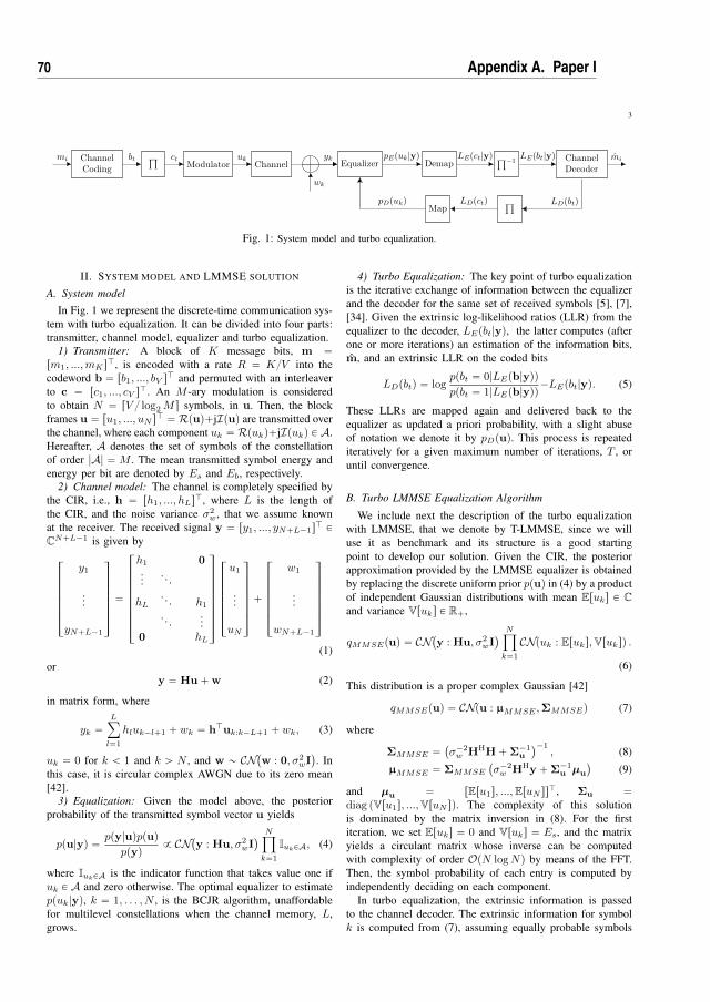
3

ChannelCoding

śModulator Channel Equalizer Demap

ś´1 ChannelDecoder

Mapś

mi bt ct uk

wk

yk pEpuk|yq LEpct|yq LEpbt|yq mi

LDpbtqLDpctqpDpukq

Fig. 1: System model and turbo equalization.

II. SYSTEM MODEL AND LMMSE SOLUTION

A. System model

In Fig. 1 we represent the discrete-time communication sys-tem with turbo equalization. It can be divided into four parts:transmitter, channel model, equalizer and turbo equalization.

1) Transmitter: A block of K message bits, m “rm1, ...,mKsJ, is encoded with a rate R “ K{V into thecodeword b “ rb1, ..., bV sJ and permuted with an interleaverto c “ rc1, ..., cV sJ. An M -ary modulation is consideredto obtain N “ rV { log2M s symbols, in u. Then, the blockframes u “ ru1, ..., uN sJ “ Rpuq`jIpuq are transmitted overthe channel, where each component uk “ Rpukq`jIpukq P A.Hereafter, A denotes the set of symbols of the constellationof order |A| “ M . The mean transmitted symbol energy andenergy per bit are denoted by Es and Eb, respectively.

2) Channel model: The channel is completely specified bythe CIR, i.e., h “ rh1, ..., hLsJ, where L is the length ofthe CIR, and the noise variance σ2

w, that we assume knownat the receiver. The received signal y “ ry1, ..., yN`L´1sJ PCN`L´1 is given by

»—————–

y1

...

yN`L´1

fiffiffiffiffiffifl“

»———————–

h1 0...

. . .

hL. . . h1. . .

...0 hL

fiffiffiffiffiffiffiffifl

»—————–

u1

...

uN

fiffiffiffiffiffifl`

»—————–

w1

...

wN`L´1

fiffiffiffiffiffifl

(1)or

y “ Hu`w (2)

in matrix form, where

yk “Lÿ

l“1

hluk´l`1 ` wk “ hJuk:k´L`1 ` wk, (3)

uk “ 0 for k ă 1 and k ą N , and w „ CN`w : 0, σ2wI

˘. In

this case, it is circular complex AWGN due to its zero mean[42].

3) Equalization: Given the model above, the posteriorprobability of the transmitted symbol vector u yields

ppu|yq “ ppy|uqppuqppyq 9 CN`y : Hu, σ2

wI˘ Nź

k“1

IukPA, (4)

where IukPA is the indicator function that takes value one ifuk P A and zero otherwise. The optimal equalizer to estimateppuk|yq, k “ 1, . . . , N , is the BCJR algorithm, unaffordablefor multilevel constellations when the channel memory, L,grows.

4) Turbo Equalization: The key point of turbo equalizationis the iterative exchange of information between the equalizerand the decoder for the same set of received symbols [5], [7],[34]. Given the extrinsic log-likelihood ratios (LLR) from theequalizer to the decoder, LEpbt|yq, the latter computes (afterone or more iterations) an estimation of the information bits,m, and an extrinsic LLR on the coded bits

LDpbtq “ logppbt “ 0|LEpb|yqqppbt “ 1|LEpb|yqq´LEpbt|yq. (5)

These LLRs are mapped again and delivered back to theequalizer as updated a priori probability, with a slight abuseof notation we denote it by pDpuq. This process is repeatediteratively for a given maximum number of iterations, T , oruntil convergence.

B. Turbo LMMSE Equalization Algorithm

We include next the description of the turbo equalizationwith LMMSE, that we denote by T-LMMSE, since we willuse it as benchmark and its structure is a good startingpoint to develop our solution. Given the CIR, the posteriorapproximation provided by the LMMSE equalizer is obtainedby replacing the discrete uniform prior ppuq in (4) by a productof independent Gaussian distributions with mean Eruks P Cand variance Vruks P R`,

qMMSEpuq “ CN`y : Hu, σ2

wI˘ Nź

k“1

CNpuk : Eruks,Vruksq .(6)

This distribution is a proper complex Gaussian [42]

qMMSEpuq “ CNpu : µMMSE ,ΣMMSEq (7)

where

ΣMMSE “`σ´2w HHH`Σ´1

u

˘´1, (8)

µMMSE “ ΣMMSE

`σ´2w HHy `Σ´1

u µu

˘(9)

and µu “ rEru1s, ...,EruN ssJ, Σu “diag pVru1s, ...,VruN sq. The complexity of this solutionis dominated by the matrix inversion in (8). For the firstiteration, we set Eruks “ 0 and Vruks “ Es, and the matrixyields a circulant matrix whose inverse can be computedwith complexity of order OpN logNq by means of the FFT.Then, the symbol probability of each entry is computed byindependently deciding on each component.

In turbo equalization, the extrinsic information is passedto the channel decoder. The extrinsic information for symbolk is computed from (7), assuming equally probable symbols


4

for the a priori information of the k-th one. By using thisturbo scheme in the receiver, the equalizer is fed back withthe statistics Eruks and Vruks, which are obtained from theupdated a priori probability pDpukq in Fig. 1 as

Epukq “ÿ

uPAu ¨ pDpuk “ uq, (10)

Vpukq “ÿ

uPApu´ Eruksq˚ pu´ Eruksq ¨ pDpuk “ uq. (11)

At this point, it is important to remark that since the variancesare no longer equal, the matrix to invert in (8) is not circulant.Therefore, the complexity of its inversion is of order OpN2Lq,as discussed later in this paper.

III. EXPECTATION PROPAGATION

Expectation propagation [26]–[28], [43] is a techniquein Bayesian machine learning to approximate an intractableprobability distribution, in which inference is unfeasible, byexponential family distributions. Suppose we are given somestatistical distribution with hidden variables x and observablesD that factors as

ppx|Dq 9 fpxqIź

i“1

tipxq, (12)

where fpxq belongs to an exponential family F with sufficientstatistics Φpxq, and tipxq are nonnegative factors that donot belong to F , making direct inference over (12) notpossible. EP provides a feasible approximation to ppx|Dq byan exponential distribution qpxq from F which factorizes as

qpxq 9 fpxqIź

i“1

tipxq, (13)

where factors tipxq P F are optimized to achieve an accu-rate global approximation qpxq Ð ppx|Dq, which optimallysatisfies EqpxqrΦpxqs “ Eppx|DqrΦpxqs. This is known as themoment matching solution. A feasible algorithm to approxi-mate this solution is the sequential EP algorithm [26], [27],which optimizes each factor tipxq in turns independently inthe context of all of the remaining factors. A sketch of theEP algorithm is given in Algorithm 1 where qr`spxq is theapproximation to qpxq in (13) at iteration `.

IV. BLOCK-EP TURBO EQUALIZER

The EP is endowed with a great flexibility, given by themodel in (13). In order to improve the accuracy of the EPsolution, it is important to retain as much structure as possiblefrom the true distribution and separate it from the latent (un-known) factors, tipxq [26]. Bearing this in mind, we developan EP approximation to (4), namely the posterior distributionof the transmitted symbols given the channel outcome y.

A. The BEP equalizerThe following Gaussian exponential family will be consid-

ered to find a suitable approximation to (4):

qpuq 9 CN`y : Hu, σ2wI

˘ Nź

k“1

exp pu˚kγk ` γ˚kuk ´ Λku˚kukq,

(15)

Algorithm 1 The EP algorithm

Initialize approximating factors tipxq and then qpxq in (13).repeat

for i “ 1, ..., I do1) Compute the distribution

pipxq 9 tipxqqr`szipxq “ tipxqqr`spxq{tr`si pxq (14)

and its moments, where qr`szipxq is the so called cavityfunction.2) Compute the refined factor t r``1s

i pxq by setting themoments of the distribution t r``1s

i pxqqr`szipxq equal tothe moments of pipxq.

end foruntil convergence (or stopped criterion)

where the product of indicator functions is replaced by aproduct of univariate proper complex Gaussians, each param-eterized by a pγk,Λkq pair, k “ 1, . . . , N . For any valueγk P C and Λk P R`, qpuq is also proper complex GaussianCNpu : µ,Σq with

Σ “ R´1 “ pσ´2w HHH` diagpΛqq´1, (16)

µ “ Σpσ´2w HHy ` γq, (17)

exhibiting a similar structure to the LMMSE in (7). Basedon these definitions in mind, we adapt the EP algorithm inAlgorithm 1 to our setting. We denote the resulting algorithmblock-EP (BEP) soft equalizer, and it can be found in Algo-rithm 2. A few remarks:

‚ Step 1) is the “LMMSE” step of the algorithm, as itrequires computing Σ and µ in (16) and (17) for thecurrent configuration of pΛ,γq. Note that this step isequivalent to the LMMSE method in (10) and (11).

‚ Steps 2.1)-2.3) can be done in parallel for k “1, . . . , N . They can be seen as a refinement to theestimate computed at Step 1) by enforcing a dis-crete distribution. Given the factorization in (15),marginal qr`spukq, k “ 1, . . . , N is proportional toexp pu˚kγk ` γ˚kuk ´ Λku

˚kukq. This term is canceled out

in pr`spukq and the“true” discrete factor is introduced. Pa-rameters canceled are recomputed by moment matchingin (22)-(23). Eqn. (22) and (23) are proposed followingthe guidelines in [36, Eq. 35-36]. The parameter update in(22) may return a negative value for some k’s. For thosek’s, we keep the values from the previous iteration. Weintroduce a smoothing parameter β P r0, 1s and a smallconstant ε. To avoid numerical instabilities, constant εis the minimum allowed variance at each iteration, i.e.,σ2r`spk “ maxpε, σ2r`s

pk q.A block diagram of the BEP equalizer is included in Fig. 2

(a). The LMMSE block corresponds to Step 1). The grey blockrepresents the refinement of the current marginals qr`spukqthrough projection over discrete alphabet, whose output is fedback to the LMMSE block.

71

5

LMMSE Demapyk ppuk|yq Lpbt|yq

S loops uk P A ChannelDecoder

mi

Block-EP equalizer

LMMSE

ComputepEpuk|yq+ Demap

Map

yk ppuk|yq LEpbt|yq

pDpukqS loops T loops

uk P A ChannelDecoder

mi

LDpbtq

Inner Turbo Equalizer (BEP)

Outer Turbo Equalizer

(a) (b)

Fig. 2: In (a), BEP equalizer block diagram. In (b), Turbo BEP block diagram.

B. The Turbo BEP equalizerThe BEP equalizer can be further improved by using a turbo

scheme. The resulting proposed equalizer, denoted as T-BEP,

Algorithm 2 Block-EP equalizer (BEP)

Input: pγr1sk ,Λr1sk q initialization.

for ` “ 1, ..., S do1) Calculate the moments of qr`spuq in (15) for the currentvalues of γk Ð γ

r`sk and Λk Ð Λ

r`sk .

for k “ 1, ..., N do2.1) Compute the k-th marginal of the distributionqr`spuq, denoted as qr`spukq “ CN

úk : µ

r`sk , σ

2r`sk

¯,

and the distribution

qr`szkpukq “ qr`spukqexp

ú˚kγ

r`sk ` γr`sk

˚uk ´ Λ

r`sk u˚kuk

¯ ∼

∼ CNúk : z

r`sk , v

2r`sk

¯, (18)

namely cavity marginal function, where

v2r`sk “ σ

2r`sk

1´ σ2r`sk Λ

r`sk

, zr`sk “ v

2r`sk

˜µr`sk

σ2r`sk

´ γr`sk

¸.

2.2) Obtain the distribution pr`spukq 9 qr`szkpukqIukPAand estimate its mean µr`spk and variance σ2r`s

pk .2.3) Set the mean and variance of the unnormalizedGaussian distribution

qr`szkpukq expú˚kγ

r``1sk,new ` γr``1s

k,new

˚uk ´ Λ

r``1sk,newu

˚kuk

¯

(19)equal to µr`spk and σ2r`s

pk . To this end, compute:

Λr``1sk,new “

´σ´2r`spk

´ v´2r`sk

¯, (20)

γr``1sk,new “

´µr`spk

σ´2r`spk

´ zr`sk v´2r`sk

¯. (21)

2.4) Update the values as

Λr``1sk “ βΛ

r``1sk,new ` p1´ βqΛr`sk , (22)

γr``1sk “ βγ

r``1sk,new ` p1´ βqγr`sk . (23)

end forend forWith the values γrS`1s,ΛrS`1s obtained after EP algorithm,calculate the final distribution qpuq in (15).

Algorithm 3 Block-EP turbo equalizer (T-BEP)

0) Initialize pγr1sk ,Λr1sk q “ p0, E´1

s q.for t “ 1, . . . , T do

1) With the current initialization to pγr1sk ,Λr1sk q, run BEP

equalizer in Algorithm 2.2) Compute an estimate to the extrinsic LLRs, LEpbt|yq,by feeding

pEpuk|yq “ qrS`1szkpukq (24)

to the demapper. Feed LEpbt|yq to the channel decoder.3) From the channel decoder per-bit soft output, recom-pute a probability distribution for each symbol pDpukqfrom the decoder and compute its mean Eruks andvariance Vruks given by (10) and (11).4) Re-initialize pγr1sk ,Λ

r1sk q to pEruksVruks´1,Vruks´1q.

end for

can be easily described as the T-LMMSE in Subsection II-Bby just replacing (7) with the result of the BEP, Algorithm 2,in (15). A detailed implementation of the T-BEP is includedin Algorithm 3. Also, a block diagram is included in Fig. 2(b).Note that the T-BEP can actually be seen as a turbo equalizerwith two loops. First we run an inner turbo scheme, i.e. BEP.After S iterations of the BEP iterative procedure, the extrinsicLLR is given to the decoder in an outer loop, which is repeatedT times. We propose to approximate the extrinsic probabilitiesby the cavity functions at the end of the EP algorithm, see (18).In this second stage the restrictions from the channel codingare exploited. The output of the channel decoder is used toinitialize the BEP iterative procedure, whose outputs are thenfed forward to the channel decoder. This is a major differencewith respect to the previous scheme used in [5], [32], [34],where the estimates were refined only using the output of thedecoder, as shown in Fig. 1, and the proposed inner loop wasnot present.

C. Efficient implementation

All pγr`sk ,Λr`sk q pairs for k “ 1, ..., N can be updated in

parallel. The most involved step is the computation of anN -dimensional inverse matrix in (16) for each `-iteration,whose complexity is dominated by its size, i.e., OpN3q. Oncethis inverse is computed, the parallel update of all pairspγr`sk ,Λ

r`sk q Ð pγr``1s

k ,Λr``1sk q by means of step 2 and 3 in


6

Algorithm 3 has a smaller computational complexity, linear inNM . To reduce the complexity of the matrix inversion, wepropose to exploit the banded structure of the channel matrixalong with the short length of the channel compared to N . Thematrix R in (16) is a symmetric, positive-definite and bandedmatrix with bandwidth 2L ´ 1. We can decompose R usingthe band Cholesky factorization [44] such that

R “ GGJ, (25)

where G is a lower triangular banded matrix with bandwidth Lthat can be computed with NL2 operations. Then, the inverseof the covariance matrix can be rewritten as

Σ “ R´1 “ G´1JG´1. (26)

We invert matrix G by Gauss-Jordan elimination. For everydiagonal element, say Gk,k, we divide row k of less than Nnon-null elements by Gk,k and cancel all the L ´ 1 lowerelements of its column. Repeated for the whole diagonal yieldsa complexity of OpN2Lq.

D. Convergence

Although the convergence is not guaranteed, we concludedempirically that in about S “ 10 iterations the distributionqpuq constructed in (15) tipically reaches a stationary value.Experimental results show that controlling numerical insta-bilities in the parameter updates in the turbo case (T ą 0)is simply done by setting ε “ 10´9 and β “ 0.1. Thissolution is robust regardless the constellation order, SNR orchannel realization. In the equalization case (T “ 0), we havefound that results can be improved if ε is first kept constantto a relatively high constant (0.5) to then reduce it. Moreprecisely, we have used ε “ 2´maxp`´5,1q. For equalizing 64-QAM constellations, the best performance has been reportedby setting fixed to ε “ 0.9. We have selected the previousvalues after extensive experimentation as a trade off betweenconvergence speed and accuracy. We emphasize again that thelatter heuristics to control stability in the equalization case arenot needed if the turbo scheme is used, as the feedback loopnaturally stabilizes the BEP output. In Fig. 3, we include arepresentative example of the convergence by depicting theevolution of some components of the mean vector µ in (17)and covariance matrix Σ in (16) along different values of Sin the low-Eb{N0 regime (specifically, Eb{N0 “ 3 dB) fora given observation, y, with a 16-PAM modulation, L “ 4and T “ 0. As shown in Fig. 3, approximately after S “ 10iterations the EP equalizer reaches a stationary value for themean and variance, equal to the value provided by the optimalBCJR approach.

E. Performance analysis

We compare probabilistic equalizers using the mutual in-formation between the transmitted symbol uk and detectedsymbol uk, distributed according to the estimation of theposterior distribution of uk given y:

Ipuk, ukq “ÿ

uk

ÿ

uk

ppuk, ukq log2

ppuk|ukqppukq , (27)

0 5 10 15 20 25 30´3

´2

´1

EP iteration ℓ(a)

Mean BEP

BCJR

0 5 10 15 20 25 307

8

9

10

EP iteration ℓ(b)

Variance

BEP

BCJR

Fig. 3: Evolution of the mean (a) and variance (b) of 3 randomlychosen entries of the approximate posterior as EP iterates with16-PAM, L “ 4 and Eb{N0 “ 3 dB.

0 5 10 15 20 251

2

3

4

5

6

Eb{N0 (dB)

Ipu

k,u

kq

BEPLMMSE

10 11 12 133

3.5

4

4.5

5

Fig. 4: Mutual information for BEP and LMMSE for 64-QAM andrandom channels with L “ 7.

where note that ppuk, ukq is the joint probability distributionof uk and uk after marginalizing the channel output y, thechannel impulse response (in the case we consider it random)and the rest of symbols in the sequence u. We resort toMonte Carlo estimates to generate samples from ppuk, ukq andthen evaluate Ipuk, ukq from these samples. We assume thatthe channel taps are Gaussian distributed, but are perfectlyknown at the receiver. First, we collect N P Z` samplesfrom the joint distribution of u,h,y and uk using standardsampling techniques in directed graphical models [43]. Thekey aspect is to note that, during the sampling procedure,ppuk|yq is dependent on the considered probabilistic detectionmethod. After N samples of possible puk, ukq pairs have beencollected, we use these samples to estimate ppukq, ppuk|ukqand, finally, Ipuk, ukq in (27). The higher Ipuk, ukq is foreach probabilistic equalizer, the closer we perform to channelcapacity. In Fig. 4 we depict the mutual information in (27)

73

7

computed for N “ 106 samples per Eb{N0 point and averagedover all the symbols in the transmitted sequence, for the BEPand LMMSE algorithms, considering a 64-QAM constellationand channels of L “ 7 complex-valued taps. Observe that,for very small Eb{N0, the noise is so large that both methodsachieve a small mutual information. On the other hand, forvery large Eb{N0 values, both methods converge to 6 bits,i.e., the number of bits transmitted per QAM symbol. Anyprobabilistic method will eventually saturate to this value.However, the key aspect is to be able to design a probabilisticequalizer able to improve the mutual information for interme-diate Eb{N0 values. Observe that before the saturation, theBEP achieves a gain w.r.t. LMMSE of around 1.5dB.

F. Computational Complexity

A detailed comparison of the complexity for the T-BEP andthe T-LMMSE is included in Table I. We also include thecomputational complexity of the T-BCJR and its approximatedapproaches with turbo. From the computational point of view,as M and/or L grow, the BCJR and approximated approachesare unaffordable.

Algorithm Complexity

T-BEP S′(LN2 +NM) + α+ S′T (LN2 + α)T-LMMSE N logN + α+ T (LN2 + α)T-BCJR (T + 1)(NML + α)

Approx. T-BCJR (T + 1)(NMeM + α)

TABLE I: Complexity comparison between algorithms, where S1 “S ` 1 and α is the complexity of the LDPC decoder.

V. EXPERIMENTAL RESULTS

In this section, we illustrate the good performance of theBEP equalizer for different scenarios. Each channel tap is i.i.d.complex circular Gaussian distributed with zero mean andvariance equal to 1{L. The channel response is normalized.We average the BER over 1000 random frames per channelrealization. We limit to 5 the absolute value of LLRs givento the decoder in order to avoid very confident probabilitieswhich negatively affect its estimations. In the following, whenmentioning approximated BCJR algorithms we refer to the M-BCJR [14], M*-BCJR [15], RS-BCJR [10], NZ and NZ-OS[17] solutions. We denote by NZ the approach consisting inrunning FT, BT or DT-NZ in [17] depending on the phaseof the channel. If output saturation is used we refer to themas NZ-OS. We use a (3,6)-regular LDPC of rate 1/2, for amaximum of 200 iterations using the belief propagation asdecoder [45], [46]. The codes were generated using the pro-gressive edge-growth algorithm [47]. The maximum number ofiterations of the LDPC decoder is set to 100 in every iterationof the turbo equalizer.

A. BEP soft equalizer

In Fig. 5 and Fig. 6 we show a comparison for some typicalchannels found in the literature using codewords of V “ 1024bits. In Fig. 5 we simulate the following scenario in [17]:

6.5 7 7.5 8

10´3

10´2

10´1

Eb{N0 (dB)BER

Fig. 5: BER for LMMSE (Ź), BEP (˝), BCJR (˛), M-BCJR (˝),M*-BCJR (˚), RS-BCJR (‹), NZ (Ÿ) and NZ-OS (‚) equalizers forBPSK and the minimum phase channel h “ 1?

140r7 6 5 4 3 2 1sJ.

6 6.5 7 7.5 8

10´3

10´2

10´1

Eb{N0 (dB)

BER

Fig. 6: BER for LMMSE (Ź), BEP (˝), BCJR (˛), M-BCJR (˝),M*-BCJR (˚), RS-BCJR (‹), NZ (Ÿ) and NZ-OS (‚) equalizers forBPSK and the maximum phase channel h “ 1?

140r1 2 3 4 5 6 7sJ.

minimum phase channel h “ r7 6 5 4 3 2 1sJ{?140, BPSKsymbols and Me “ 4 states out of 64. In Fig. 6 we simulatethe maximum phase channel h “ r1 2 3 4 5 6 7sJ{?140and BPSK symbols with Me “ 8 states for the approximatedsolutions as in [17]. To study the performance for otherchannels, in Fig. 7 and Fig. 8 we include the averaged BERover 100 random channels with L “ 5 real-valued taps. Wefix to Me “ 8 the number of states for the approximatedsolutions. In Fig. 7, we consider BPSK modulation, hence theBCJR has 16 states per step, while in Fig. 8 a 4-PAM is used,increasing the number of states to 256.

In Fig. 5 and Fig. 6 we can observe that approximatedmethods M-BCJR, M*-BCJR, RS-BCJR are quite sensitiveto the channel realization. This is not only caused becausethey are based on just a forward or a backward strategy, butalso because their parameters need to be tuned according tothe particular channel. For this reason, the approximations M-BCJR, M*-BCJR and RS-BCJR fail with maximum phase


8

5 6 7 8 9 10 11 12

10´4

10´3

10´2

10´1

Eb{N0 (dB)

BER

Fig. 7: BER for LMMSE (Ź), BEP (˝), BCJR (˛), M-BCJR (˝),M*-BCJR (˚), RS-BCJR (‹), NZ (Ÿ) and NZ-OS (‚) equalizers forBPSK and 100 random channels with L “ 5.

10 12 14 16 18 2010´5

10´4

10´3

10´2

10´1

Eb{N0 (dB)

BER

Fig. 8: BER for LMMSE (Ź), BEP (˝), BCJR (˛), M-BCJR (˝),M*-BCJR (˚), RS-BCJR (‹), NZ (Ÿ) and NZ-OS (‚) equalizers for4-PAM and 100 random channels with L “ 5.

channels, as observed in Fig. 6. For averaged channels, seeFig. 7, NZ and NZ-OS exhibit a good performance at a lowcomputational complexity due to the low state reduction ratio(ML{Me). However, these solutions fail if Me does not growaccordingly, as can be observed in Fig. 8. This means that ifthe number of states, Me, is kept as a fraction of the totalnumber, ML, they may exhibit a good performance. But if alarge number of states is unaffordable, a fraction of it becomesalso intractable. The LMMSE in these experiments does notfail as the approximated approaches do, but its performancedegrades significantly compared to the BER of the BCJR inFig. 8. Finally, the BEP exhibits a quite robust behavior, closerto the BCJR performance. Note here that the number of statesis low, and that the BCJR can be used with optimal results ata low complexity.

For multilevel constellations and a channel with a few taps,the BCJR or their approximations are no longer computation-ally affordable. In the case of large dimensions, filter-basedequalizers of the MMSE type are preferred [20]. In Fig. 9,

8 10 12 14 16 18 20 22 24

10´4

10´3

10´2

10´1

Eb{N0 (dB)

BER

LMMSE

BEP

CS

Fig. 9: BER for LMMSE (Ź), BEP (˝) and CS (‹) equalizers for16-QAM (solid lines) and 64-QAM (dashed lines) and 100 randomchannels with L “ 7.

we depict the BER curves for BEP, LMMSE equalization andthe algorithm in [19] that we denote as channel shortening(CS), considering codewords of V “ 4096 bits, 100 randomchannels of L “ 7 complex-valued taps and two differentmodulations: 16-QAM (solid lines) and 64-QAM (dashedlines). The CS algorithm has been simulated with a reducedmemory ν “ 2 (ν “ 1) for the 16-QAM (64-QAM) case. Weobserve in this experiment that the BEP exhibits significantimprovements with respect to the LMMSE and CS solutionfor both constellations.

B. Turbo BEP

To improve the estimates the turbo-equalization can be used.We simulate scenarios with large dimensions, where the onlycomputationally feasible algorithms are the BEP and LMMSEsolutions. In Fig. 10 we simulate a 16-QAM constellation,averaging over 100 random channels with a large memory,L “ 20 complex-valued taps and codewords of V “ 1024 bits.We represent the first 3 iterations of the turbo scheme, sincewe found no further improvement for T ě 3. In Fig. 11 andFig. 12, we depict the BER curves for turbo BEP and LMMSEequalization, averaged over 100 random channels of L “ 7complex-valued taps, 64-QAM modulation and codewords ofV “ 1024 and V “ 4096 bits, respectively, for T “ 3.

The results are remarkable. The BEP with no feedback fromthe decoder is 1.5-4.5 dB away from the LMMSE equalizerfor BER=10´4, depending on the channel length, L, and theconstellation size, M . It even outperforms the turbo LMMSEequalizer. The BEP estimation can be further improved usingthe turbo scheme, in about 1 or 1.5 dB depending on thecodeword length.

VI. CONCLUSIONS

When the number of states involved in the BCJR equaliza-tion or its approximations is high, their computational com-plexity is unaffordable. Approximated strategies are interestingwhenever the number of states is not too high. Therefore,

75

9

8 9 10 11 12 13

10´4

10´3

10´2

10´1

Eb{N0 (dB)

BER

T-BEP

T-LMMSE

Fig. 10: BER for T-BEP (red lines, solid) and T-LMMSE (blue lines,dashed) equalizers using the outer loop for 16-QAM and 100 randomchannels with L “ 20. No feedback (˝), one loop (Ÿ), two loops (˝)and three loops (`).

16 18 20 22 24

10´4

10´3

10´2

10´1

Eb{N0 (dB)

BER

T-BEP

T-LMMSE

Fig. 11: BER for T-BEP (red lines, solid) and T-LMMSE (blue lines,dashed) equalizers using the outer loop for 64-QAM, 100 randomchannels with L “ 7 and codewords of V “ 1024 bits. No feedback(˝), one loop (Ÿ), two loops (˝) and three loops (`).

in the case of multilevel constellations with moderate orlarge channel lengths, it is preferable to resort to MMSEtype equalizers. The turbo LMMSE equalization improvesthe estimations by feeding back the output of the channeldecoder to the equalizer. In this paper we propose the EP as anovel alternative, where the whole posterior probabilities areapproximated in a complex-valued formulation. This equalizer,denoted as BEP, can be cast as an LMMSE with an innerturbo scheme. The BEP exploits the fact that the transmittedsymbols belong to a known constellation to improve theestimations. This soft equalizer outperforms the turbo LMMSEequalization. The BEP equalization can be further improvedby exploiting the channel decoder output to propose the turboBEP equalizer. This can be interpreted as an outer turboequalization as compared to the proposed EP based inner turboequalization. In the included experiments, we report gains inthe range 1.5-5 dB with respect to the LMMSE. We have

16 18 20 22 24

10´4

10´3

10´2

10´1

Eb{N0 (dB)BER

T-BEP

T-LMMSE

Fig. 12: BER for T-BEP (red lines, solid) and T-LMMSE (blue lines,dashed) equalizers using the outer loop for 64-QAM, 100 randomchannels with L “ 7 and codewords of V “ 4096 bits. No feedback(˝), one loop (Ÿ), two loops (˝) and three loops (`).

focused on block or batch solutions, to report computationalcomplexities of orderOpN2Lq. The development of windowedor filtered solutions remains as future research, to reduce thecomputational complexity to be linear in the frame length.

REFERENCES

[1] R. Schober, “Detection and estimation of signals in noise,” Universityof British Columbia, Vancouver, Tech. Rep., 2010.

[2] J. G. Proakis, Digital Communications, 5th ed. New York, NY:McGraw-Hill, 2008.

[3] S. Haykin, Communication Systems, 5th ed. Wiley Publishing, 2009.[4] L. Salamanca, J. J. Murillo-Fuentes, and F. Perez-Cruz, “Bayesian

equalization for LDPC channel decoding,” IEEE Trans. on SignalProcessing, vol. 60, no. 5, pp. 2672–2676, May 2012.

[5] M. Tuchler and A. Singer, “Turbo equalization: An overview,” IEEETrans. on Information Theory, vol. 57, no. 2, pp. 920–952, Feb 2011.

[6] C. Douillard, M. Jezequel, C. Berrou, P. Didier, and A. Picart, “Iterativecorrection of intersymbol interference: turbo-equalization,” EuropeanTrans. on Telecommunications, vol. 6, no. 5, pp. 507–512, Sep 1995.

[7] R. Koetter, A. Singer, and M. Tuchler, “Turbo equalization,” IEEE SignalProcessing Magazine, vol. 21, no. 1, pp. 67–80, Jan 2004.

[8] L. Bahl, J. Cocke, F. Jelinek, and J. Raviv, “Optimal decoding of linearcodes for minimizing symbol error rate (corresp.),” IEEE Trans. onInformation Theory, vol. 20, no. 2, pp. 284–287, 1974.

[9] F. Kschischang, B. Frey, and H.-A. Loeliger, “Factor graphs and thesum-product algorithm,” IEEE Trans. on Information Theory, vol. 47,no. 2, pp. 498 –519, Feb 2001.

[10] G. Colavolpe, G. Ferrari, and R. Raheli, “Reduced-state BCJR-typealgorithms,” IEEE Journal on Sel. Areas in Communications, vol. 19,no. 5, pp. 848–859, May 2001.

[11] M. Eyuboglu and S. Qureshi, “Reduced-state sequence estimation withset partitioning and decision feedback,” IEEE Trans. on Communica-tions, vol. 36, no. 1, pp. 13–20, Jan 1988.

[12] A. Duel-Hallen and C. Heegard, “Delayed decision-feedback sequenceestimation,” IEEE Trans. on Communications, vol. 37, no. 5, pp. 428–436, May 1989.

[13] P. Chevillat and E. Eleftheriou, “Decoding of trellis-encoded signals inthe presence of intersymbol interference and noise,” IEEE Trans. onCommunications, vol. 37, no. 7, pp. 669–676, Jul 1989.

[14] V. Franz and J. Anderson, “Concatenated decoding with a reduced-search BCJR algorithm,” IEEE Journal on Selected Areas in Communi-cations, vol. 16, no. 2, pp. 186–195, Feb 1998.

[15] M. Sikora and D. Costello, “A new SISO algorithm with applicationto turbo equalization,” in Proc. IEEE International Symposium onInformation Theory (ISIT), Sep 2005, pp. 2031–2035.


10

[16] C. Vithanage, C. Andrieu, and R. Piechocki, “Approximate inferencein hidden Markov models using iterative active state selection,” IEEESignal Processing Letters, vol. 13, no. 2, pp. 65–68, Feb 2006.

[17] D. Fertonani, A. Barbieri, and G. Colavolpe, “Reduced-complexityBCJR algorithm for turbo equalization,” IEEE Trans. on Communica-tions, vol. 55, no. 12, pp. 2279–2287, Dec 2007.

[18] J. G. Proakis and D. G. Manolakis, Digital Signal Processing: Princi-ples, Algorithms, and Applications, 2nd ed. Prentice Hall, 1996.

[19] F. Rusek and A. Prlja, “Optimal channel shortening for MIMO and ISIchannels,” IEEE Trans. on Wireless Communications, vol. 11, no. 2, pp.810–818, Feb 2012.

[20] C. Berrou, Codes and turbo codes, ser. Collection IRIS. Springer Paris,2010.

[21] G. Colavolpe and G. Germi, “On the application of factor graphs andthe sum-product algorithm to ISI channels,” IEEE Trans. on Communi-cations, vol. 53, no. 5, pp. 818–825, May 2005.

[22] J. Hu, H. Loeliger, J. Dauwels, and F. Kschischang, “A generalcomputation rule for lossy summaries/messages with examples fromequalization,” in Proc. 44th Allerton Conf. Communication, Control, andComputing, Sep 2006, pp. 27–29.

[23] Q. Guo and L. Ping, “LMMSE turbo equalization based on factorgraphs,” IEEE Journal on Selected Areas in Communications, vol. 26,no. 2, pp. 311–319, Feb 2008.

[24] G. Colavolpe, D. Fertonani, and A. Piemontese, “SISO detection overlinear channels with linear complexity in the number of interferers,”IEEE Journal of Selected Topics in Signal Processing, vol. 5, no. 8, pp.1475–1485, Dec 2011.

[25] P. Sun, C. Zhang, Z. Wang, C. Manchon, and B. Fleury, “Iterativereceiver design for ISI channels using combined belief- and expectation-propagation,” IEEE Signal Processing Letters, vol. 22, no. 10, pp. 1733–1737, Oct 2015.

[26] T. P. Minka, “A family of algorithms for approximate Bayesian infer-ence,” Ph.D. dissertation, Massachusetts Institute of Technology, 2001.

[27] T. Minka, “Expectation propagation for approximate Bayesian infer-ence,” in Proc. 17th Conference on Uncertainty in Artificial Intelligence(UAI), 2001, pp. 362–369.

[28] M. Seeger, “Expectation propagation for exponential families,” Univ.Calif., Berkeley, CA, USA, Tech. Rep., 2005.

[29] K. Muranov, “Survey of MMSE channel equalizers,” University ofIllinois, Chicago, Tech. Rep.

[30] J. Wu and Y. Zheng, “Low complexity soft-input soft-output block deci-sion feedback equalization,” in Proc. IEEE Global TelecommunicationsConference (GLOBECOM), Nov 2007, pp. 3379–3383.

[31] S. Kim, J. Lee, and Y. Kim, “Adaptive Cholesky based MMSE equalizerin GSM,” in Proc. IEEE Asia Pacific Conference on Circuits and Systems(APCCAS), Nov 2008, pp. 886–889.

[32] M. Tuchler, A. Singer, and R. Koetter, “Minimum mean squarederror equalization using a priori information,” IEEE Trans. on SignalProcessing, vol. 50, no. 3, pp. 673–683, Mar 2002.

[33] L. Liu and L. Ping, “An extending window MMSE turbo equalizationalgorithm,” IEEE Signal Processing Letters, vol. 11, no. 11, pp. 891–894, Nov 2004.

[34] M. Tuchler, R. Koetter, and A. Singer, “Turbo equalization: principlesand new results,” IEEE Trans. on Communications, vol. 50, no. 5, pp.754–767, May 2002.

[35] M. Senst and G. Ascheid, “How the framework of expectation propa-gation yields an iterative IC-LMMSE MIMO receiver,” in Proc. IEEEGlobal Telecommunications Conference (GLOBECOM), Dec 2011, pp.1–6.

[36] J. Cespedes, P. M. Olmos, M. Sanchez-Fernandez, and F. Perez-Cruz,“Expectation propagation detection for high-order high-dimensionalMIMO systems,” IEEE Trans. on Communications, vol. 62, no. 8, pp.2840–2849, Aug 2014.

[37] J. Cespedes, P. M. Olmos, M. Sanchez-Fernandez, and F. Perez-Cruz,“Improved performance of LDPC-coded MIMO systems with EP-basedsoft-decisions,” in Proc. IEEE International Symposium on InformationTheory (ISIT), Jun 2014, pp. 1997–2001.

[38] P. M. Olmos, J. J. Murillo-Fuentes, and F. Perez-Cruz, “Tree-structureexpectation propagation for LDPC decoding over the BEC,” IEEE Trans.on Information Theory, vol. 59, no. 6, pp. 3354–3377, 2013.

[39] L. Salamanca, P. M. Olmos, F. Perez-Cruz, and J. J. Murillo-Fuentes,“Tree-structured expectation propagation for LDPC decoding over BMSchannels,” IEEE Trans. on Communications, vol. 61, no. 10, pp. 4086–4095, Oct 2013.

[40] Y. Qi and T. Minka, “Window-based expectation propagation for adap-tive signal detection in flat-fading channels,” IEEE Trans. on WirelessCommunications, vol. 6, no. 1, pp. 348–355, Jan 2007.

[41] I. Santos, J. J. Murillo-Fuentes, and P. M. Olmos, “Block expectationpropagation equalization for ISI channels,” in Proc. 23rd EuropeanSignal Processing Conference (EUSIPCO), Sep 2015, pp. 379–383.

[42] P. J. Schreier and L. L. Scharf, Statistical Signal Processing of Complex-Valued Data. The Theory of Improper and Noncircular Signals. Cam-bridge, UK: Cambridge University Press, 2010.

[43] C. M. Bishop, Pattern Recognition and Machine Learning (InformationScience and Statistics). Secaucus, NJ, USA: Springer-Verlag, NewYork, 2006.

[44] G. H. Golub and C. F. Van Loan, Matrix Computations, 3rd ed.Baltimore, MD, USA: Johns Hopkins University Press, 1996.

[45] T. J. Richardson and R. Urbanke, Modern Coding Theory. CambridgeUniversity Press, Mar. 2008.

[46] L. Salamanca, J. J. Murillo-Fuentes, P. M. Olmos, F. Perez-Cruz, andS. Verdu, “Approaching the DT bound using linear codes in the shortblocklength regime,” IEEE Communications Letters, vol. 19, no. 2, pp.123–126, Feb 2015.

[47] X.-Y. Hu, E. Eleftheriou, and D. M. Arnold, “Regular and irregularprogressive edge-growth tanner graphs,” IEEE Trans. on InformationTheory, vol. 51, no. 1, pp. 386–398, 2005.

77

Appendix BPaper II

Authors: Irene Santos, Juan José Murillo-Fuentes, Eva Arias de Reyna and PabloM. Olmos.Title: Turbo EP-based Equalization: a Filter-Type Implementation.Journal: IEEE Transactions on Communications.Date: September 2017.Status: Accepted.Abstract: We propose a novel filter-type equalizer to improve the solution of thelinear minimum-mean squared-error (LMMSE) turbo equalizer, with computa-tional complexity constrained to be quadratic in the filter length. When high-ordermodulations and/or large memory channels are used the optimal BCJR equalizeris unavailable, due to its computational complexity. In this scenario, the filter-type LMMSE turbo equalization exhibits a good performance compared to otherapproximations. In this paper, we show that this solution can be significantly im-proved by using expectation propagation (EP) in the estimation of the a posterioriprobabilities. First, it yields a more accurate estimation of the extrinsic distributionto be sent to the channel decoder. Second, compared to other solutions based onEP the computational complexity of the proposed solution is constrained to bequadratic in the length of the finite impulse response (FIR). In addition, we reviewprevious EP-based turbo equalization implementations. Instead of consideringdefault uniform priors we exploit the outputs of the decoder. Some simulationresults are included to show that this new EP-based filter remarkably outperformsthe turbo approach of previous versions of the EP algorithm and also improves theLMMSE solution, with and without turbo equalization.

79

1

Turbo EP-based Equalization: a Filter-TypeImplementation

Irene Santos, Juan Jose Murillo-Fuentes, Eva Arias-de-Reyna, and Pablo M. Olmos

Abstract—We propose a novel filter-type equalizer to im-prove the solution of the linear minimum-mean squared-error(LMMSE) turbo equalizer, with computational complexity con-strained to be quadratic in the filter length. When high-ordermodulations and/or large memory channels are used the optimalBCJR equalizer is unavailable, due to its computational complex-ity. In this scenario, the filter-type LMMSE turbo equalizationexhibits a good performance compared to other approximations.In this paper, we show that this solution can be significantlyimproved by using expectation propagation (EP) in the estimationof the a posteriori probabilities. First, it yields a more accurateestimation of the extrinsic distribution to be sent to the channeldecoder. Second, compared to other solutions based on EP thecomputational complexity of the proposed solution is constrainedto be quadratic in the length of the finite impulse response (FIR).In addition, we review previous EP-based turbo equalizationimplementations. Instead of considering default uniform priorswe exploit the outputs of the decoder. Some simulation resultsare included to show that this new EP-based filter remarkablyoutperforms the turbo approach of previous versions of the EPalgorithm and also improves the LMMSE solution, with andwithout turbo equalization.

Index Terms—Expectation propagation (EP), linear MMSE,low-complexity, turbo equalization, ISI, filter-type equalizer.

I. INTRODUCTION

MANY digital communication systems need to transmitover channels that are affected by inter-symbol interfer-

ence (ISI). The equalizer produces a probabilistic estimation ofthe transmitted data given the vector of observations [1]. Sig-nificant improvements are found when the previous estimationis given to a probabilistic channel decoder [2]. Equalizationcan be done in the frequency domain to avoid complexityproblems associated with the inverse of covariance matrices[3]. In addition, feeding the equalizer back again with theoutput of the decoder, iteratively, yields a turbo-equalizationscheme that significantly reduces the overall error rate [4]–[6].

The BCJR algorithm [7] performs optimal turbo equal-ization under the maximum a posteriori (MAP) criterion. Itprovides a posteriori probability (APP) estimations given some

I. Santos, J.J. Murillo-Fuentes and E. Arias-de-Reyna are with the Dept.Teorıa de la Senal y Comunicaciones, Escuela T. Superior de Ingenierıa,Universidad de Sevilla, Camino de los Descubrimiento s/n, 41092 Sevilla,Spain. E-mail: {irenesantos,murillo,earias}@us.es

P. M. Olmos is with the Dept. Teorıa de la Senal y Comunicaciones,Universidad Carlos III de Madrid, Avda. de la Universidad 30, 28911, Leganes(Madrid), Spain. He is also with the Instituto de Investigacion SanitariaGregorio Maranon (IiSGM). E-mail: [email protected].

The final version of the manuscript can be found athttps://ieeexplore.ieee.org/document/8353388/. Thiswork was partially funded by Spanish government (Ministerio de Economıay Competitividad TEC2016-78434-C3-{2-3}-R and Juan de la Cierva GrantNo. IJCI-2014-19150) and by the European Union (FEDER).

a priori information about the transmitted data. However, itscomplexity grows exponentially with the length of the channeland the constellation size, becoming intractable for few tapsand/or multilevel constellations. In this situation, approximatedBCJR solutions, such as [8]–[11], can be used. They arebased on a search over a simplified trellis with only Me

states, yielding a complexity which is linear in this numberof states. However, the performance of these approaches isquite dependent on the channel realization and the order ofthe constellation used. In addition, these approximated BCJRsolutions degrade rapidly if the number of survivor paths doesnot grow according to the total number of states. For thesereasons, filter-based equalizers are preferred [12].

A quite extended filter type equalizer in the literature isbased on the well-known linear minimum-mean squared-error(LMMSE) algorithm [5], [13], [14]. This LMMSE filter isan appealing alternative where the BCJR is computationallyunfeasible due to its robust performance with linear complex-ity in the frame length, N, and quadratic dependence withthe window length, W. From a Bayesian point of view, theLMMSE algorithm obtains a Gaussian extrinsic distributionby replacing the discrete prior distribution of the transmittedsymbols with a Gaussian prior.

A more accurate estimation for the extrinsic distribution canbe obtained by replacing the prior distributions with approx-imations of the probability distribution. This can be done bymeans of the expectation propagation (EP) algorithm. The EPapproach projects the approximated posterior distribution intothe family of Gaussians by matching its moments iterativelywith the ones of the true posterior. This algorithm has beenalready successfully applied to multiple-input multiple-output(MIMO) systems [15] and low-density parity-check (LDPC)channel decoding [16], [17], among others. It has been alsoapplied to turbo equalization in a message passing approachas a way to incorporate into the BP algorithm the discrete in-formation coming from the channel decoder [18], [19]. Thesemessage passing methods reduce to the LMMSE estimationif no turbo equalization is employed. A different approach isproposed in [20], [21] under the name of block EP (BEP)where, rather than applying EP after the channel decoder, it isused within the equalizer to better approximate the posterior,outperforming previous solutions.

The computational complexity of previous EP-based equal-izers is large for long frame lengths or memories of the chan-nel. Due to its block implementation, the complexity of theBEP is quadratic in the frame length, becoming intractable forlarge frames [21]. To overcome this drawback, a smoothing EP(SEP) implementation is proposed in [22], but its complexity

80 Appendix B. Paper II

2

is cubic with the memory of the channel. Furthermore, due totheir iterative procedure, their computational load is roughlyS times the one of the LMMSE counterparts, where S isthe number of iterations used in the EP algorithm, typicallyaround 10 [15], [20], [21]. Besides, in both, BEP and SEP,uniform discrete priors are assumed for the constellation ofthe modulations when computing the EP approximations, evenwithin the turbo equalization iterations, while the use ofinformation from the decoder remains unexplored.

The results developed in this paper focus on improving theseprevious EP-based equalizers [21], [22] both in computationalcomplexity and performance. First, we improve the prior infor-mation used in the equalizer once the turbo procedure starts,forcing the true discrete prior to be non-uniform in contrast tothe uniform priors used by previous EP-based approaches. Asa result, we achieve a performance improvement. Second, thecomputational complexity of the EP algorithm is reduced toroughly a third part of that in [21], by optimizing the choiceof EP parameters. Third, and most important, a new filter-typeEP solution is designed. This solution is constrained to havelinear complexity in the frame length and quadratic in the filterlength, i.e., it is endowed with the same complexity order thanthe LMMSE filter.

The novel EP-based filter proposed outperforms theLMMSE algorithm with a robust behavior to changes in theconstellation size and the channel realization, as the BEP andSEP approaches do [21], [22]. In the experiments included, weshow that the EP filter solution greatly improves the LMMSEsolution with and without turbo equalization, specifically wehave 2 dB gains for a BPSK, 5 dB for the 8-PSK and 6-13 dBfor 16 and 64-QAM, respectively. In comparison with previousEP approaches, the EP filter matches their performance withBPSK constellations, and outperforms them with gains of 2dBs for 8-PSK and 4-5 dBs for 16 and 64-QAM. We studythe extrinsic information transfer (EXIT) charts [5], [23] ofour proposal for a BPSK, where the EP-based filter achievesthe same performance as the BEP.

The scope of this paper encompasses time domain equal-ization. Frequency domain equalization has received a lot ofattention as it usually achieves a complexity reduction for theblock-wise processing [3], [14], [24], [25]. For this reason,derivation of a frequency domain counterpart for the proposedEP based turbo-equalizer remains as a future research line.Another promising research route is the application to MIMOwith channels with memory [3], [26], [27].

The paper is organized as follows. We first describe inSection II the model of the communication system at hand.Section III is devoted to develop a new implementation of theEP-based equalizer considering non-uniform priors and studiesthe optimal values for the parameters. In Section IV, we reviewthe formulation for the LMMSE filter in turbo equalizationand describe the novel EP filter-type solution proposed. InSection VI, we include several simulations to compare bothEP and LMMSE approaches. We end with conclusions.

Through the paper, we denote the i-th entry of a vector u asui, its complex conjugate as u˚ and its Hermitian transposeas uH. We define δpuiq as the delta function that takes valueone if ui “ 0 and zero in other case. We use CNpu : µ,Σq

to denote a normal distribution of a random proper complexvector u with mean vector µ and covariance matrix Σ.

II. SYSTEM MODEL

The model of the communication system is depicted inFig. 1, including turbo equalization at the receiver. There arethree main blocks: transmitter, channel and turbo receiver.

A. Transmitter

The information bit sequence, a “ ra1, ..., aKsJ where ai Pt0, 1u, is encoded into the coded bit vector b “ rb1, ..., bV sJwith a code rate equal to R “ K{V . After permuting thebits with an interleaver, the codeword c “ rc1, ..., cV sJis partitioned into N blocks of length Q “ log2pMq, c “rc1, ..., cNsJ where ck “ rck,1, ..., ck,Qs, and modulated witha complex M-ary constellation A of size |A| “ M. Thesemodulated symbols, u “ ru1, ..., uNsJ, where each componentuk “ Rpukq ` jIpukq P A, are transmitted over the channel.Hereafter, transmitted symbol energy and energy per bit aredenoted as Es and Eb, respectively.

B. Channel

The channel is completely specified by the CIR, i.e., h “rh1, ..., hLsJ, where L is the number of taps, and is corruptedwith AWGN whose noise variance, σ2

w, is known. Each k-thentry of the complex received signal y “ ry1, ..., yN`L´1sJ isgiven by

yk “Lÿ

j“1

hjuk´j`1 ` wk “ hJuk:k´L`1 ` wk, (1)

where wk „ CN`wk : 0, σ2

w

˘and uk “ 0 for k ă 1 and k ą N.

C. Turbo receiver

When no information is available from the channel decoder,the posterior probability of the transmitted symbol vector ugiven the whole vector of observations y yields

ppu|yq 9 ppy|uqppuq (2)

where, assuming equiprobable symbols, the prior would begiven by

ppuq “ 1

M

Nź

k“1

ÿ

uPAδpuk ´ uq. (3)

This prior matches with the definition given in [21] but, asexplained below, it is just valid before the turbo procedure.

In a turbo architecture the equalizer and decoder iterativelyexchange information for the same set of received symbols[5], [14]. Traditionally, this exchange of information is donein terms of extrinsic probabilities in order to improve conver-gence and avoid instabilities. The extrinsic information at theoutput of the equalizer (see Fig. 1), pEpuk|yq, is computedso as to meet the turbo principle [13]. These probabilities,pEpuk|yq, are approximated when the optimal solution isintractable. We will denote the approximation by qEpukq.

81

3

ChannelCoder

śModulator H(z) Equalizer

Demapϕp¨q

ś´1 ChannelDecoder

śMap

ai bt ct uk

wk

yk pEpuk|yq LEpctq LEpbtq pai

LDpbtqLDpctqpDpukq


Fig. 1: System model.

The extrinsic distributions are demapped,

LEpck,jq “ log

řukPA|ck,j“0 pEpuk|yqřukPA|ck,j“1 pEpuk|yq

, (4)

deinterleaved and given to the decoder as extrinsic log-likelihood ratios, LEpbtq. The channel decoder computes anestimation of the information bits, pa, along with the extrinsicLLRs on the coded bits, computed as

LDpbt|LEpbqq “ logppbt “ 0|LEpbqqppbt “ 1|LEpbqq´LEpbtq. (5)

These extrinsic LLRs are interleaved, mapped again and givento the equalizer as updated priors, pDpu|LEpbqq, which arecomputed as

pDpuk|LEpbqq “ÿ

uPAδpukúq

Qź

j“1

pDpck,j “ ϕjpuq|LEpbqq,(6)

with ϕjpuq denoting the j-th bit associated to the demappingof symbol u. This process is repeated iteratively for a givenmaximum number of iterations, T , or until convergence.Note that in Fig. 1 we have included the computation ofthe extrinsic information within the equalization and channeldecoding blocks. Note also that, once the turbo procedurestarts, the prior in (2) is conditioned on the input at the channeldecoder and the symbols are not equiprobable anymore. In thissituation, the posterior distribution computed by the equalizeris given by

ppu|yq 9 ppy|uqNź

k“1

pDpuk|LEpbqq, (7)

The true posterior distribution in (2) and (7) has complexityproportional to ML. When this complexity becomes intractable,we will approximate it, denoting it as qpuq. In the following,we omit the dependence on the input at the decoder, LEpbq,to keep the notation uncluttered in the rest of the paper. It isalso uncluttered in Fig. 1.

III. NON-UNIFORM BEP TURBO EQUALIZER

EP [28]–[32] is a technique in Bayesian machine learningthat approximates a (non-exponential) distribution with an ex-ponential distribution whose moments match the true ones. Inthis paper, we focus on computing a Gaussian approximationfor the posterior in (7), which is clearly non Gaussian due tothe product of discrete priors in (6). As introduced in [21],this is done by iteratively updating an approximation within

the Gaussian exponential family by replacing the non Gaussianprior terms in (2) by a product of Gaussians1, i.e.,

qr`spuq 9 ppy|uqNź

k“1

pr`sD pukq

“ CN`y : Hu, σ2wI

˘ Nź

k“1

CNúk : m

r`sk , η

r`sk

¯(8)

The marginalization of the resulting approximated Gaussianposterior distribution for the k-th transmitted symbol and `-thEP iteration yields

qr`spukq „ CNúk : µ

r`sk , s

2r`sk

¯(9)

where

µr`sk “ m

r`sk ` (10)

` ηr`sk hkH´σ2wI`Hdiagpηr`sqHH

¯´1 py ´Hmr`sq,

s2r`sk “ η

r`sk ´ η2r`sk hk

H´σ2wI`Hdiagpηr`sqHH

¯´1

hk,

(11)

H is the N` L´ 1ˆ N channel matrix given by

H “

»——————————–

h1 0 . . . 0...

. . . . . ....

hL. . . 0

0. . . h1

.... . . . . .

...0 . . . 0 hL

fiffiffiffiffiffiffiffiffiffiffifl

(12)

and hk is the k-th column of H (see Appendix A for thedemonstration). At this point it is interesting to remark that (9)-(11) are completely equivalent to equations (15)-(17) in [21].Here we developed the values of the mean and variance foreach symbol while in [21] they were computed in block form.The current description is simpler because we only includethe elements of the covariance matrix that are used duringthe execution of the algorithm, excluding the non-diagonalelements.

1Note that in [21] we used an alternative expression for (8) (an exponentialdistribution with parameters γk “ mk{ηk and Λk “ 1{ηk).


4

The mean and variance parameters in (8) are initialized withthe statistics from the channel decoder as

mr1sk “

ÿ


ηr1sk “

ÿ

uPApu´mr1sk q˚pu´mr1sk q ¨ pDpuk “ uq. (14)

Then, they are updated in parallel and iteratively by matchingthe moments of the following distributions

qr`sE pukqpDpukq

momentmatchingÐÑ q

r`sE pukqCN

úk : m

r``1sk , η

r``1sk

¯

(15)where qr`sE pukq is an extrinsic marginal distribution computedas2

qr`sE pukq “ qr`spukq{pr`sD pukq “ CN

úk : z

r`sk , v

2r`sk

¯(16)

where

zr`sk “ µ

r`sk η

r`sk ´mr`sk s

2r`sk

ηr`sk ´ s2r`sk

, (17)

v2r`sk “ s

2r`sk η

r`sk

ηr`sk ´ s2r`sk

. (18)

Note that this equalizer differs from the one in [21] becausewe used different definitions for the true prior, pDpukq. In thecurrent manuscript, we considered non-uniform and discretepriors, given by (6), during the moment matching procedurein the equalizer, while in [21] uniform priors as in (3) wereconsidered by default even after the turbo procedure. Toincrease the accuracy of the algorithm, a damping procedurefollows the moment matching in (15). We have defined analgorithm, described in Algorithm 1, called Moment Matchingand Damping that runs these two procedures.

A. The nuBEP algorithm

Algorithm 2 contains a detailed description of the whole EPprocedure, where S is the number of EP iterations while T isthe number of turbo iterations. Note that the difference with theapproach in [21] lies in the definition of the prior distributionused during the moment matching procedure. In [21], we usean uniform distribution (denoted with the indicator function),forcing the same a priori probability for the symbols, regard-less of the information fed back from the decoder, during themoment matching employed in the equalizer even after theturbo procedure starts. In this paper, we refine the definitionof the prior used in the moment matching of EP algorithm as in(6), considering non-uniform priors once the turbo procedurestarts. For this reason, we named this algorithm non-uniformBEP (nuBEP) turbo equalizer.

2Note that in this paper we used qr`sE pukq to denote the extrinsic marginal

distribution, while in [21] we denoted as qr`szkpukq and called it cavitymarginal function.

Algorithm 1 Moment Matching and Damping

Given inputs: µr`spk , σ2r`spk , z

r`sk , v

2r`sk ,m

r`sk , η

r`sk

1) Run moment matching: Set the mean and variance of theunnormalized Gaussian distribution

qr`sE pukq ¨ CN

úk : m

r``1sk,new, η

r``1sk,new

¯(19)

equal to µr`spk and σ2r`spk , to get the solution

ηr``1sk,new “

σ2r`spk v

2r`sk

v2r`sk ´ σ2r`s

pk

, (20)

mr``1sk,new “ η

r``1sk,new

˜µr`spk

σ2r`spk

´ zr`sk

v2r`sk

¸. (21)

2) Run damping: Update the values as

ηr``1sk “

˜β

1

ηr``1sk,new

` p1´ βq 1

ηr`sk

¸´1

, (22)

mr``1sk “ η

r``1sk

˜βmr``1sk,new

ηr``1sk,new

` p1´ βqmr`sk

ηr`sk

¸. (23)

if ηr``1sk ă 0 then

ηr``1sk “ η

r`sk , m

r``1sk “ m

r`sk . (24)

end ifOutput: ηr``1s

k ,mr``1sk

B. On the election of EP parameters

The moment matching condition explained in (15) deter-mines the optimal operation point found by the EP approxima-tion. By repeating this procedure, we allow to find a stationarysolution for the operation point. In order to avoid instabilitiesand control the accuracy and speed of convergence, some EPparameters are introduced. These parameters are the numberof EP iterations (S), a minimum allowed variance (ε) anda damping factor (β). Based on recent studies, these EPparameters can be further optimized [33]–[35]. Following theguidelines in those papers and after extensive experimentation,in the general case we found out that instabilities can becontrolled by setting3 ε “ 1e´8. Regarding the accuracy ofthe algorithm, it is convenient to start with a conservativevalue of the damping parameter β in Algorithm 2. The valueβ “ 0.1 forces our algorithm to move slowly towards the EPsolution. Once the turbo procedure starts, we let the dampingparameter grow in order to speed up the achievement of the EPsolution, reducing the value of S from 10 in [21] to 3. A simplerule for determination of β that fulfills this requirements andleads to good performance is an exponential growth witha saturation value of 0.7, i.e., β “ minpexpt{1.5 {10q, 0.7q,where t P r0, T s is the number of the current turbo iteration.With this criterion the number of EP iterations after the turboprocedure starts is reduced to S “ 3, hence reducing thecomputational complexity by more than a third.

3Parameters have been chosen to optimize turbo equalization [35].

83

5

Algorithm 2 nuBEP Turbo EqualizerInitialization: Set pDpukq “ 1

M

řuPA δpuk ´ uq for k “

1, . . . , Nfor t “ 1, ..., T do

1) Compute the mean mr1sk and variance η

r1sk given by

(13) and (14), respectively.for ` “ 1, ..., S do

for k “ 1, ..., N do2) Compute the k-th extrinsic distribution as in (16),i.e.,

qr`sE pukq “ CN

´uk : z

r`sk , v

2r`sk

¯(25)

where zr`sk and v

2r`sk are given by (17) and (18),

respectively.3) Obtain the distributionppr`spukq 9 q

r`sE pukqpDpukq and estimate its

mean µr`spk and variance σ

2r`spk . Set a minimum

allowed variance as σ2r`spk “ maxpε, σ2r`s

pk q.4) Run the moment matching and damping proce-dures by executing Algorithm 1.

end forend for5) With the values mrS`1s

k , ηrS`1sk obtained after the EP

algorithm, calculate the extrinsic distribution qEpukq.6) Demap the extrinsic distribution and compute theextrinsic LLR, LEpck,jq, by means of (4).7) Run the channel decoder to output pDpukq

end forOutput: Deliver LEpck,jq to the channel decoder for k “1, . . . , N and j “ 1, . . . , Q

IV. FILTER-TYPE TURBO EQUALIZATION

A. LMMSE filter

In this subsection we review the formulation of theLMMSE-based filter [5], [13], [14], modified to allow forunnormalized transmitted energy and a different computationof the extrinsic distribution. The LMMSE-based filter [5],[13], [14] estimates one symbol per k-th iteration, uk, givena W-size window of observations, yk “ ryk´W2 , ..., yk`W1sJ,where W “ W1`W2`1. This procedure differs from [36], whereeach transmitted symbol is estimated given the whole vectorof observations, y. The LMMSE equalizer approximates theprior for each symbol, pDpukq, as a Gaussian

pDpukq « pDpukq “ CNpuk : mk, ηkq , (26)

where the mean, mk, and variance, vk, are a priori statistics foreach transmitted symbol, given by (13) and (14), respectively.For the first iteration of the turbo equalization no a prioriinformation is available and a suitable initialization is mk “ 0,ηk “ Es, which boils down to mk “ 0, ηk “ 1 whennormalizing the energy [5], [13], [14]. Given the currentprior and the channel impulse response (CIR), the LMMSEfilter computes a Gaussian approximation of the posteriorprobability of each symbol. When a turbo scheme is used,the equalizer and decoder exchange extrinsic information [6].

Through the turbo equalization iterations, the a priori statisticsin (26) are updated with the information fed back from thechannel decoder.

Rather than computing the posterior distribution as in (7),the LMMSE filter [5] considers the a posteriori probabilitieswith respect to the estimated transmitted symbol, puk. Forthis reason, and to keep the same notation than in [5], wewill denote the approximated posterior as qpuk|pukq. With thisposterior distribution in mind, the extrinsic probability at theoutput of the LMMSE filter can be computed as

qEpuk|pukq “ qpuk|pukqpDpukq . (27)

This distribution is Gaussian and can be derived from theextrinsic distribution of the estimated symbol computed in [5],as shown in Appendix B, yielding

qEpuk|pukq “ CN`uk : zk, v

2k

˘(28)

where

zk “ ckHpyk ´HWmk `mkhWq

ckHhW

, (29)

v2k “ck

HhWEsp1´ hWHckq

pckHhWq2 , (30)

and, in turn,

ck “´Σk ` pEs ´ ηkqhWhW

H¯´1

EshW, (31)

HW “

»————–

hL . . . h1 0. . . . . .

. . . . . .0 hL . . . h1

fiffiffiffiffifl

(32)

is the W ˆ pW ` L ´ 1q channel matrix, hW is the (W2 ` L)-thcolumn of HW and

mk “ rmk´L´W2`1, ...,mk`W1sJ, (33)Vk “ diagpηk´L´W2`1, ..., ηk`W1q, (34)

Σk “ σ2wI`HWVkHW

H. (35)

The computational complexity is dominated by (31), which hasto be recomputed every k-th iteration. Hence, the complexityis OpNW2q. This complexity can be further reduced by relyingon some approximations proposed in [5], [14].

B. EP filter (EP-F)

A novel EP filter-type is developed in this subsection toimprove the accuracy and performance of the LMMSE-basedfilter explained above. As explained in Subsection IV-A,if the LMMSE filter is run, the prior of each symbol isapproximated by a Gaussian with the statistics given by thedecoder, i.e., with mean and variance given by (13) and(14), respectively. By using the EP algorithm we approximatethe posterior distribution with a Gaussian family. Since theposterior distribution includes the true discrete priors, we takeinto account the discrete nature of symbols.

At every iteration of the EP algorithm, `, we approximatethe product of priors of individual symbols in (7) as a product


6

Algorithm 3 EP-FInitialization: Set pDpukq “ 1

M


1, . . . , Nfor t “ 1, ..., T do

1) Compute the mean mr1sk and variance η

r1sk given by

(13) and (14), respectively.for ` “ 1, ..., S do

for k “ 1, ..., N do2) Compute the k-th extrinsic distribution as in (28),i.e.,

qr`sE puk|pukq “ CN

´uk : z

r`sk , v

2r`sk

¯(37)

where zr`sk and v

2r`sk are given by (29) and (30),

respectively.3) Obtain the distributionppr`spukq 9 q

r`sE puk|pukqpDpukq and estimate its

mean µr`spk and variance σ

2r`spk . Set a minimum

allowed variance as σ2r`spk “ maxpε, σ2r`s

pk q.4) Run the moment matching and damping proce-dures by executing Algorithm 1.

end forend for5) With the values mrS`1s

k , ηrS`1sk obtained after the EP

algorithm, calculate the extrinsic distribution qEpuk|pukqin (28).6) Demap the extrinsic distribution and compute theextrinsic LLR, LEpck,jq, by means of (4).7) Run the channel decoder to output pDpukq

end forOutput: Deliver LEpck,jq to the channel decoder for k “1, . . . , N and j “ 1, . . . , Q

of N Gaussians, pr`sD pukq “ CN´uk : m

r`sk , η

r`sk

¯, whose pa-

rameters (means and variances) are adjusted to find a betterapproximation, qr`spuq 9 ppy|uqśN

k“1 pr`sD pukq, to the true

posterior. Similarly to (27)-(28), for each k-th symbol, we firstcompute the current extrinsic distribution,

qr`sE puk|pukq “

qr`spuk|pukqpr`sD pukq

. (36)

Now, a more accurate posterior distribution can be obtained byfinding a new Gaussian approximation, pr``1s

D pukq, to matchthe moments of qr`sE puk|pukqpr``1s

D pukq and qr`sE puk|pukqpDpukq,as in (15). With these new values for the mean, mr``1s

k , andvariance, ηr``1s

k , we can recompute a new extrinsic distributionqr``1sE puk|pukq, which is more accurate than the one in (28).

The final extrinsic distribution delivered to the decoder isthe one obtained after the last iteration of the EP algorithm,following (36).

We denote this new algorithm as EP-filter (EP-F). Algo-rithm 3 is a detailed description of its implementation. Notethat the main difference between Algorithm 2 and Algorithm 3lies in the computation of the extrinsic distribution, i.e.,equations (25) and (37). The computational complexity is alsodominated by (31), which has to be computed for each symbol

and each `-th iteration. Hence, the complexity is S times theLMMSE complexity, i.e. OpSNW2q, where S is the number ofiterations of the EP-F. At this point, it is interesting to remarkthat the approximations proposed in [5], [14] to further reducethe complexity cannot be applied when the EP is used. Thereason is that these approximations remove (at some points)the prior variance computed by the decoder, setting it to one.

V. RELATION TO PREVIOUS APPROACHES

A. Update of the priors

We improve the prior information used in the equalizer oncethe turbo procedure starts, forcing the true discrete prior to benon-uniform in contrast to the uniform priors used by previousEP-based approaches.

In previous proposals [20]–[22], the probabilities from thechannel decoder, pDpukq, were used to initialize, at thebeginning of every iteration of the turbo-equalization, theproduct of Gaussians that in the EP approximation replaces theproduct of priors, pr1sD pukq. But when the moment matchingwas performed in the EP algorithm, i.e.,

qr`sE pukqIukPA


r`sE pukqpr``1s

D pukq, (38)

the true priors used were uniformly distributed following

IukPA “1

M

ÿ

uPAδpuk ´ uq. (39)

In the current proposal, we keep the initialization of theGaussians in every step of the turbo-equalization, pr1sD pukq,but also propose to replace the uniform priors in (39) by non-uniform ones in the moment matching step, as explained in(15), i.e.,

qr`sE pukqpDpukq


r`sE pukqpr``1s

D pukq, (40)

where

pDpukq “ÿ

uPAδpuk ´ uq

Qź

j“1

pDpck,j “ ϕjpuqq, (41)

Note that the different definition of priors -(39) in previousproposals, (41) in this manuscript- is the difference betweenthe currently proposed nuBEP algorithm and the BEP in [21],with remarkable improvements.

B. Parameter Optimization

The computational complexity of the EP algorithm is re-duced to roughly a third part of that in [21], by optimizingthe choice of EP parameters. In particular, we propose somenew values for ε and β, that control numerical instabilities inthe EP updates, and S, the number of iterations of the EPequalizer. The parameters proposed in this paper reduce thenumber of iterations in turbo equalization to S “ 3, ratherthan the S “ 10 iterations that were used in [21].

85

7

C. Filter-type solution

The new filter-type EP solution proposed is constrained tohave linear complexity in the frame length and quadratic inthe filter length, i.e., it is endowed with the same complexityorder than the LMMSE filter. This complexity is not quadraticwith the block length as the one of the BEP [21] nor cubicwith the window length as complexity of the SEP [22].

D. Equalization solved with EP

Regarding the EP-based equalizers proposed by other au-thors, the approach in [18], [19] should be mentioned. Theseproposals deal just with how to pass information between thechannel decoder and the LMMSE equalizer. Our proposal firstfocuses on the EP based equalization, performed indepen-dently of the turbo iterations. Therefore the approaches arequite different. Issues such as how to use the priors in themoment matching within the EP equalizer or the damping donot arise in these proposals where the improvement is relatedonly to the handling of probabilities between blocks.

VI. SIMULATION RESULTS

In this section, we compare the performance of both theblock LMMSE and EP-F equalizers for different scenarios.We also include the performance of the BEP [21] and theAWGN bound as references. Note that the MMSE filter [5]has not been included in the simulations since the blockLMMSE exhibits equal or better performance than any fil-tering approaches based on the LMMSE algorithm. We didnot include the SEP algorithm since it exhibits the sameperformance as the block implementation, as shown in [22].We also include the nuBEP approach to illustrate the quiteimproved behavior when using non-uniform priors at each EPiteration, even reducing from 10 to 3 the number of iterationsof the EP approach. The EP parameters have been selected asexplained in Subsection III-B, both for the nuBEP and EP-F methods. For a full performance comparison with BCJRapproximations, such as M-BCJR [8], M*-BCJR [10], RS-BCJR [9], NZ and NZ-OS [11], please see [21]. In Table Iwe include a detailed comparison of the complexity of all thesimulated algorithms. Above we include the computationalcomplexity of previous algorithms in [21] (BEP) and [22](SEP), the block and filter implementation of the LMMSE andBCJR approaches. Below we provide the complexity for thenew approaches in this paper, i.e., the proposed nuBEP andEP-F. Parameter W is typically around two times the lengthof the channel, L. Here, we simulate the scenarios in [13],[14], using the same channel responses and modulations. Othermodulations are also considered. The absolute value of LLRsgiven to the decoder is limited to 5 in order to avoid veryconfident probabilities. We use a (3,6)-regular LDPC of rate1/2, and belief propagation as decoder with a maximum of100 iterations. The window length in the filtered approach isset to W “ W1 ` W2 ` 1, where W1 “ 2L and W2 “ L ` 1 assuggested in [14].

In the following, we first include a section to analyze theperformance of our approach in a low complexity scenariowith BPSK modulation, similarly to [14]. The optimal BCJR

TABLE I: Complexity comparison between algorithms.

AlgorithmComplexity perturbo iteration

BCJR NML

BEP 10LN2

block-LMMSE LN2

SEP 10NW3

LMMSE filter NW2

nuBEP 3LN2

EP-F 3NW2

algorithm can be run in this scenario with a low enoughcomputational complexity and is used as bound. Next, weinclude a section to analyze the behavior of the algorithmsin a large complexity scenario, where we use high-ordermodulations such as 8-PSK, 16-QAM and 64-QAM.

A. BPSK scenario

In Fig. 2 we include the BER, averaged over 104 ran-dom frames, for the LMMSE, BEP [21], nuBEP, EP-F andBCJR equalizers with a BPSK modulation and two differ-ent channel responses and lengths of encoded words: h “r0.227 0.46 0.688 0.46 0.227sJ and V “ 4096 bits in Fig. 2(a)-(c) and h “ r0.407 0.815 0.407sJ and V “ 1024 bits inFig. 2 (d)-(f). The channel responses were selected followingthe simulations in [13], [14]. The performances of block-algorithms, BEP and nuBEP, are very similar to the equivalentforward filtering approach. When the nuBEP algorithm is ap-plied, 2 and 1.5 dBs gains are obtained compared to LMMSEapproach in the turbo scenario, for the two simulated scenarios,respectively. The EP-F exhibits a performance similar to thatof the nuBEP.

In Fig. 3 we include the EXIT charts of the BEP [21],nuBEP, EP-F, LMMSE and BCJR for the channel responseh “ r0.227 0.46 0.688 0.46 0.227sJ as in [5], [13], BPSKmodulation with Eb{N0 “ 9 (solid) and 7 dB (dashed).The EXIT chart of the LDPC encoder of 2048{4096 andR “ 1{2 used is also depicted (solid). The horizontal andvertical axis depict the mutual information at the input, Ii,and the output, Io, respectively. We use arrows to show theevolution of the mutual information along the turbo iterationsfor Eb{No “ 9 dB. Vertical (horizontal) arrows indicate theimprovement in the mutual information each time the equalizer(channel decoder) is executed. When no a priori information isgiven to the decoder, i.e., Ii “ 0, both BEP and EP-F provide ahigher value for the mutual information at the output, Io, thanthe LMMSE approach, i.e., they start from a more accurateestimation even before the turbo equalization. This greatlyimproves the performance as it enlarges the gap between theequalizer and the channel decoder EXIT curves. It can be seenthat the LMMSE approach will fail when Eb{No “ 7 dB,because both curves intersect.

Note that the wide EXIT tunnel from the equalizer to theLDPC decoder is suggesting that the code is not optimum interms of capacity [37]. An optimal code in this sense would


8

0 5 10 1510´5

10´4

10´3

10´2

10´1

Eb{N0 (dB)

BER

Channel h “ r0.227 0.46 0.688 0.46 0.227sJ

(a) Without turbo feedback

0 5 10 1510´5

10´4

10´3

10´2

10´1

Eb{N0 (dB)

BER

(b) After two turbo loops

0 5 10 1510´5

10´4

10´3

10´2

10´1

Eb{N0 (dB)

BER

(c) After five turbo loops

2 4 6 810´5

10´4

10´3

10´2

10´1

Eb{N0 (dB)

BER

Channel h “ r0.407 0.815 0.407sJ

(d) Without turbo feedback

2 4 6 810´5

10´4

10´3

10´2

10´1

Eb{N0 (dB)

BER

(e) After two turbo loops

2 4 6 810´5

10´4

10´3

10´2

10´1

Eb{N0 (dB)

BER

(f) After five turbo loops

Fig. 2: BER along Eb{N0 for BEP [21] (˝), nuBEP (˝), EP-F (˚), block-LMMSE (Ź) and BCJR (˛) turbo equalizers, BPSK, codewords ofV “ 4096 bits (a)-(c) and V “ 1024 bits (d)-(f) and two different channel responses. Black lines represent the AWGN bound.

exhibit an EXIT chart near below the one of the equalizer andabove the curve of the 1{2 rate LDPC code used. The designof this code for the channel equalization response is out of thescope of this paper and remains as a future line of research.

B. Large complexity scenario

In Fig. 4 we simulate the same scenario of Fig. 2, but usingan 8-PSK modulation rather than a BPSK. It can be observedthat after increasing the order of the modulation, the EP-Fapproach presented in this work performs identically as itsblock counterpart, greatly improving the performance of theLMMSE algorithm before and after the turbo procedure. Animprovement of the BER of the EP-F with respect to the one

of the BEP approach in [21], after turbo equalization, can alsobe observed.

In Fig. 5 we depict the BER performance after five turboloops for channels h “ r0.227 0.46 0.688 0.46 0.227sJin (a) and h “ r0.407 0.815 0.407sJ in (b) with differentmodulations. We use solid lines to represent a 64-QAM con-stellation and dashed lines for a 16-QAM. We sent codewordsof length V “ 4096 in both scenarios. It can be observedthat the performance of the EP-F matches with the one of itsblock implementation proposed in this paper (nuBEP) whena 16-QAM is used. However, the EP-F approach slightlydegrades with a 64-QAM, where the block nuBEP gets themost accurate performance. Note that the behavior of theEP-F could be improved by increasing the length of the filter,

87

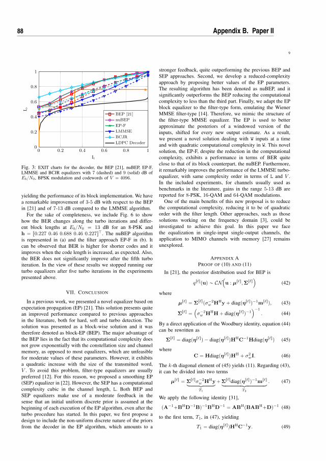
9

0 0.2 0.4 0.6 0.8 10

0.2

0.4

0.6

0.8

1

Ii

I o

BEP [21]

nuBEP

EP-F

LMMSE

BCJR

LDPC Decoder

Fig. 3: EXIT charts for the decoder, the BEP [21], nuBEP, EP-F,LMMSE and BCJR equalizers with 7 (dashed) and 9 (solid) dB ofEb{N0, BPSK modulation and codewords of V “ 4096.

yielding the performance of its block implementation. We havea remarkable improvement of 3-5 dB with respect to the BEPin [21] and of 7-13 dB compared to the LMMSE algorithm.

For the sake of completeness, we include Fig. 6 to showhow the BER changes along the turbo iterations and differ-ent block lengths at Eb{N0 “ 13 dB for an 8-PSK andh “ r0.227 0.46 0.688 0.46 0.227sJ. The nuBEP algorithmis represented in (a) and the filter approach EP-F in (b). Itcan be observed that BER is higher for shorter codes and itimproves when the code length is increased, as expected. Also,the BER does not significantly improve after the fifth turboiteration. In the view of these results we stopped running ourturbo equalizers after five turbo iterations in the experimentspresented above.

VII. CONCLUSION

In a previous work, we presented a novel equalizer based onexpectation propagation (EP) [21]. This solution presents quitean improved performance compared to previous approachesin the literature, both for hard, soft and turbo detection. Thesolution was presented as a block-wise solution and it wastherefore denoted as block-EP (BEP). The major advantage ofthe BEP lies in the fact that its computational complexity doesnot grow exponentially with the constellation size and channelmemory, as opposed to most equalizers, which are unfeasiblefor moderate values of these parameters. However, it exhibitsa quadratic increase with the size of the transmitted word,V . To avoid this problem, filter-type equalizers are usuallypreferred [12]. For this reason, we proposed a smoothing EP(SEP) equalizer in [22]. However, the SEP has a computationalcomplexity cubic in the channel length, L. Both BEP andSEP equalizers make use of a moderate feedback in thesense that an initial uniform discrete prior is assumed at thebeginning of each execution of the EP algorithm, even after theturbo procedure has started. In this paper, we first propose adesign to include the non-uniform discrete nature of the priorsfrom the decoder in the EP algorithm, which amounts to a

stronger feedback, quite outperforming the previous BEP andSEP approaches. Second, we develop a reduced-complexityapproach by proposing better values of the EP parameters.The resulting algorithm has been denoted as nuBEP, and itsignificantly outperforms the BEP reducing the computationalcomplexity to less than the third part. Finally, we adapt the EPblock equalizer to the filter-type form, emulating the WienerMMSE filter-type [14]. Therefore, we mimic the structure ofthe filter-type MMSE equalizer. The EP is used to betterapproximate the posteriors of a windowed version of theinputs, shifted for every new output estimate. As a result,we present a novel solution dealing with W inputs at a timeand with quadratic computational complexity in W. This novelsolution, the EP-F, despite the reduction in the computationalcomplexity, exhibits a performance in terms of BER quiteclose to that of its block counterpart, the nuBEP. Furthermore,it remarkably improves the performance of the LMMSE turbo-equalizer, with same complexity order in terms of L and V .In the included experiments, for channels usually used asbenchmarks in the literature, gains in the range 5-13 dB arereported for 8-PSK, 16-QAM and 64-QAM modulations.

One of the main benefits of this new proposal is to reducethe computational complexity, reducing it to be of quadraticorder with the filter length. Other approaches, such as thosesolutions working on the frequency domain [3], could beinvestigated to achieve this goal. In this paper we facethe equalization in single-input single-output channels, theapplication to MIMO channels with memory [27] remainsunexplored.

APPENDIX APROOF OF (10) AND (11)

In [21], the posterior distribution used for BEP is

qr`spuq „ CN´u : µr`s,Σr`s

¯(42)

where

µr`s “ Σr`spσ´2w HHy ` diagpηr`sq´1mr`sq, (43)

Σr`s “´σ´2w HHH` diagpηr`sq´1

¯´1

. (44)

By a direct application of the Woodbury identity, equation (44)can be rewritten as

Σr`s “ diagpηr`sq ´ diagpηr`sqHHC´1Hdiagpηr`sq (45)

whereC “ Hdiagpηr`sqHH ` σ2

wI. (46)

The k-th diagonal element of (45) yields (11). Regarding (43),it can be divided into two terms

µr`s “ Σr`sσ´2w HHyloooooomoooooonT1

`Σr`sdiagpηr`sq´1mr`sloooooooooooomoooooooooooonT2

. (47)

We apply the following identity [31],

pA´1`BHD´1Bq´1BHD´1 “ ABHpBABH`Dq´1 (48)

to the first term, T1, in (47), yielding

T1 “ diagpηr`sqHHC´1y. (49)


10

5 10 15 2010´5

10´4

10´3

10´2

10´1

Eb{N0 (dB)

BER

Channel h “ r0.227 0.46 0.688 0.46 0.227sJ

(a) Without turbo feedback

5 10 15 2010´5

10´4

10´3

10´2

10´1

Eb{N0 (dB)

BER

(b) After two turbo loops

5 10 15 2010´5

10´4

10´3

10´2

10´1

Eb{N0 (dB)

BER

(c) After five turbo loops

5 10 1510´5

10´4

10´3

10´2

10´1

Eb{N0 (dB)

BER

Channel h “ r0.407 0.815 0.407sJ

(d) Without turbo feedback

5 10 1510´5

10´4

10´3

10´2

10´1

Eb{N0 (dB)

BER

(e) After two turbo loops

5 10 1510´5

10´4

10´3

10´2

10´1

Eb{N0 (dB)

BER

(f) After five turbo loops

Fig. 4: BER along Eb{N0 for BEP [21] (˝), nuBEP (˝), EP-F (‹) and block-LMMSE (Ź) turbo equalizers, 8-PSK, codewords of V “ 4096(a)-(c) and V “ 1024 (d)-(f) and two different channel responses. Black lines represent the AWGN bound.

Now, we replace (45) into the second term, T2, in (47),obtaining

T2 “ mr`s ´ diagpηr`sqHHC´1Hmr`s. (50)

By replacing (49) and (50) into (47), we finally get

µr`s “ mr`s ` diagpηr`sqHHC´1py ´Hmr`sq, (51)

whose k-th element is given by (10).

APPENDIX BPROOF OF (29) AND (30)

In [5], the extrinsic distribution of the estimated symbol iscomputed as

qEppuk|ukq „ CN`puk : ukck

HhW, σ2k

˘(52)

where

puk “ ckHpyk ´HWmk `mkhWq, (53)

σ2k “ ck

HhWEsp1´ hWHckq, (54)

ck is given by (31) and hW is the (W2 ` L)-th column of HW

defined in (32). Note that we generalized the expressions in[5] to consider a symbol energy of Es. If we set Es “ 1, weobtain exactly the formulation in [5]. Instead of the extrinsicdistribution of the estimated symbol, we use in our formulationthe extrinsic distribution of the true symbol, which can becomputed from (52) as

qEpuk|pukq „ CN`uk : zk, v

2k

˘(55)

89

11

5 10 15 20 25 30 3510´5

10´4

10´3

10´2

10´1

Eb{N0 (dB)

BER

(a) Channel h “ r0.227 0.46 0.688 0.46 0.227sJ

5 10 15 20 2510´5

10´4

10´3

10´2

10´1

Eb{N0 (dB)BER

(b) Channel h “ r0.407 0.815 0.407sJ

Fig. 5: BER along Eb{N0 for BEP [21] (˝), nuBEP (˝), EP-F (˚) and block-LMMSE (Ź) turbo equalizers after five turbo loops, 64-QAM(solid lines) and 16-QAM (dashed lines), codewords of V “ 4096 and two different channel responses. Black lines represent the AWGNbound.

0 1 2 3 4 5 6 710´5

10´4

10´3

10´2

10´1

turbo iteration #

BER

(a) nuBEP

V “ 256

V “ 512

V “ 1024

V “ 2048

V “ 4096

V “ 8192

0 1 2 3 4 5 6 710´5

10´4

10´3

10´2

10´1

turbo iteration #

BER

(b) EP-F

V “ 256

V “ 512

V “ 1024

V “ 2048

V “ 4096

V “ 8192

Fig. 6: BER of nuBEP (a) and EP-F (b) turbo equalizers at Eb{N0 “ 13 dB for several turbo iterations and lengths of encoded words.8-PSK modulation and the channel response h “ r0.227 0.46 0.688 0.46 0.227sJ were used.

where

zk “ pukckHhW

, (56)

v2k “σ2k

pckHhWq2 , (57)

yielding the formulation in (29) and (30).

REFERENCES



[3] J. Karjalainen, N. Veselinovic, K. Kansanen, and T. Matsumoto, “Itera-tive frequency domain joint-over-antenna detection in multiuser mimo,”IEEE Transactions on Wireless Communications, vol. 6, no. 10, pp.3620–3631, October 2007.






[9] G. Colavolpe, G. Ferrari, and R. Raheli, “Reduced-state BCJR-type al-gorithms,” IEEE Journal on Selected Areas in Communications, vol. 19,no. 5, pp. 848–859, May 2001.




[13] M. Tuchler, A. Singer, and R. Koetter, “Minimum mean squarederror equalization using a priori information,” IEEE Trans. on Signal


12

Processing, vol. 50, no. 3, pp. 673–683, Mar 2002.[14] M. Tuchler and A. Singer, “Turbo equalization: An overview,” IEEE

Trans. on Information Theory, vol. 57, no. 2, pp. 920–952, Feb 2011.[15] J. Cespedes, P. M. Olmos, M. Sanchez-Fernandez, and F. Perez-Cruz,

“Improved performance of LDPC-coded MIMO systems with EP-basedsoft-decisions,” in Proc. IEEE International Symposium on InformationTheory (ISIT), Jun 2014, pp. 1997–2001.



[18] J. Hu, H. Loeliger, J. Dauwels, and F. Kschischang, “A generalcomputation rule for lossy summaries/messages with examples fromequalization,” in Proc. 44th Allerton Conf. Communication, Control, andComputing, Sep 2006, pp. 27–29.



[21] I. Santos, J. J. Murillo-Fuentes, R. Boloix-Tortosa, E. Arias-de-Reyna,and P. M. Olmos, “Expectation propagation as turbo equalizer in ISIchannels,” IEEE Trans. on Communications, vol. 65, no. 1, pp. 360–370, Jan 2017.

[22] I. Santos, J. J. Murillo-Fuentes, E. Arias-de-Reyna, and P. M. Olmos,“Probabilistic equalization with a smoothing expectation propagationapproach,” IEEE Trans. on Wireless Communications, vol. 16, no. 5,pp. 2950–2962, May 2017.

[23] K. Kansanen and T. Matsumoto, “An analytical method for mmse mimoturbo equalizer exit chart computation,” IEEE Transactions on WirelessCommunications, vol. 6, no. 1, pp. 59–63, Jan 2007.

[24] D. Falconer, S. L. Ariyavisitakul, A. Benyamin-Seeyar, and B. Eidson,“Frequency domain equalization for single-carrier broadband wirelesssystems,” IEEE Communications Magazine, vol. 40, no. 4, pp. 58–66,Apr 2002.

[25] M. Tuchler and J. Hagenauer, “Turbo equalization using frequencydomain equalizers,” in Proc. of the Allerton Conference. on Commu-nication, Control, and Computing, Oct. 2000, pp. 1234–1243.

[26] N. Veselinovic, T. Matsumoto, and M. Juntti, Iterative PDF Estimation-Based Multiuser Diversity Detection and Channel Estimation withUnknown Interference. Hindawi Publishing Corporation: EURASIPJournal on Advances in Signal Processing, 2005. [Online]. Available:https://doi.org/10.1155/ASP.2005.872

[27] L. Xiao, Y. Xiao, Y. Zhao, P. Yang, M. D. Renzo, S. Li, and W. Xiang,“Time-domain turbo equalization for single-carrier generalized spatialmodulation,” IEEE Transactions on Wireless Communications, vol. 16,no. 9, pp. 5702–5716, Sept 2017.





[32] K. Takeuchi, “Rigorous dynamics of expectation-propagation-based sig-nal recovery from unitarily invariant measurements,” in IEEE Interna-tional Symposium on Information Theory (ISIT), June 2017, pp. 501–505.

[33] M. Opper and O. Winther, “Expectation consistent approximate infer-ence,” Journal of Machine Learning Research, vol. 6, pp. 2177–2204,Dec 2005.

[34] J. Cespedes, “Approximate inference in massive mimo scenarios withmoment matching techniques,” Ph.D. dissertation, Universidad CarlosIII de Madrid, Jan 2017.

[35] J. Cespedes, P. M. Olmos, M. Sanchez-Fernandez, and F. Perez-Cruz,“Probabilistic MIMO symbol detection with expectation consistencyapproximate inference,” IEEE Trans. on Vehicular Technology, Sep2017. Accepted.

[36] J. Wu and Y. Zheng, “Low complexity soft-input soft-output block deci-sion feedback equalization,” in Proc. IEEE Global TelecommunicationsConference (GLOBECOM), Nov 2007, pp. 3379–3383.

[37] Q. Xie, Z. Yang, J. Song, and L. Hanzo, “EXIT-chart-matching-aidednear-capacity coded modulation design and a BICM-ID design examplefor both gaussian and rayleigh channels,” IEEE Transactions on Vehic-ular Technology, vol. 62, no. 3, pp. 1216–1227, March 2013.

91

Appendix CPaper III

Authors: Irene Santos, Juan José Murillo-Fuentes, Eva Arias de Reyna and PabloM. Olmos.Title: Probabilistic Equalization With a Smoothing Expectation Propagation Ap-proach.Journal: IEEE Transactions on Wireless Communications.Volume: 16.Number: 5.Pages: 2950-2962.Date: May 2017.Abstract: In this paper, we face the soft equalization of channels with inter-symbolinterference for large constellation sizes, M. In this scenario, the optimal BCJRsolution and most of their approximations are intractable, as the number of statesthey track grows fast with M. We present a probabilistic equalizer to approximatethe posterior distributions of the transmitted symbols using the expectation prop-agation (EP) algorithm. The solution is presented as a recursive sliding windowapproach to ensure that the computational complexity is linear with the lengthof the frame. The estimations can be further improved with a forward–backwardapproach. This novel soft equalizer, denoted as smoothing EP (SEP), is also testedas a turbo equalizer, with a low-density parity-check (LDPC) channel decoder.The extensive results reported reveal remarkably good behavior of the SEP. In lowdimensional cases, the bit error rate (BER) curves after decoding are closer than 1dB from those of the BJCR, robust to the channel response. For large M, the SEPexhibits gains in the range of 3-5 dB compared to the linear minimum mean squareerror algorithm.

93

1

Probabilistic Equalization with a SmoothingExpectation Propagation Approach

Irene Santos, Juan Jose Murillo-Fuentes, Eva Arias-de-Reyna, and Pablo M. Olmos

Abstract—In this paper we face the soft equalization ofchannels with inter-symbol interference for large constellationsizes, M. In this scenario the optimal BCJR solution and mostof their approximations are intractable, as the number of statesthey track grows fast with M. We present a probabilistic equalizerto approximate the posterior distributions of the transmittedsymbols using the expectation propagation (EP) algorithm. Thesolution is presented as a recursive sliding window approach toensure that the computational complexity is linear with the lengthof the frame. The estimations can be further improved with aforward-backward approach. This novel soft equalizer, denotedas smoothing expectation propagation (SEP), is also tested asturbo equalizer, with a low-density parity-check (LDPC) channeldecoder. The extensive results reported reveal remarkably goodbehavior of the SEP. In low dimensional cases, the bit error rate(BER) curves after decoding are closer than 1 dB from thoseof the BJCR, robust to the channel response. For large M, theSEP exhibits gains in the range 3-5 dB compared to the linearminimum mean square error algorithm.

Index Terms—Expectation propagation (EP), BCJR, low-complexity, turbo channel equalization, ISI.

I. INTRODUCTION

EQUALIZATION provides an estimation for the transmit-ted symbols [1], by canceling out the inter-symbol inter-

ference (ISI) [2], [3]. The probability of each possible trans-mitted symbol can be also supplied, from which nowadayschannel decoders highly benefit [4]. This soft information canbe further refined by using turbo equalization, i.e., by feedingback the output of the channel decoder to the probabilisticequalizer [5]–[7]. If the channel decoder works iteratively, thefeedback is performed after one or more iterations.

The BCJR algorithm [8] can be used as symbol maximum aposteriori (MAP) soft equalizer in schemes where a posterioriprobabilities (APP) are suitable as inputs to the channeldecoder. The BCJR assumes perfect channel state information(CSI) to work on a trellis representation [4], [9]. It exploits adoubly terminated frame where the first and last symbols are

I. Santos, J.J. Murillo-Fuentes and E. Arias-de-Reyna are with the Dept.Teorıa de la Senal y Comunicaciones, Escuela Tecnica Superior de Ingenierıa,Universidad de Sevilla, Camino de los Descubrimiento s/n, 41092 Sevilla,Spain. E-mail: {irenesantos,murillo,earias}@us.es.

P. M. Olmos is with the Dept. Teorıa de la Senal y Comunicaciones,Universidad Carlos III de Madrid, Avda. de la Universidad 30, 28911, Leganes(Madrid), Spain. E-mail: [email protected].

The final version of the manuscript can be found athttps://ieeexplore.ieee.org/document/7880668/. Thiswork was partially funded by Spanish government (Ministerio de Economıay Competitividad TEC2016-78434-C3-{2-3}-R and Juan de la Cierva GrantNo. IJCI-2014-19150), by the European Union (FEDER and Marie CurieInitial Training Network “Machine Learning for Personalized Medicine”MLPM2012, Grant No. 316861), and by Comunidad de Madrid in Spain(project ’CASI-CAM-CM’, id. S2013/ICE-2845).

known. The BCJR is based on the definition of states and thecomputation of their probabilities from previous estimationsand new observations through the trellis, in a forward filteringstep. A similar procedure is performed backwards. Finally,the estimation at a given time is computed from both filteringresults, as a smoothing approach. The BCJR has a complexityOpNMLq, i.e., linear with the frame length, N, and proportionalto the number of states, ML. The BCJR memory requirementsper step also grow exponentially, because it stores ML´1

variables and the M possible transitions from each variable tothe next one.

The complexity of the optimal BCJR solution becomesintractable in high dimensional scenarios, in particular whentransmitting multilevel constellations. To reduce its complex-ity, approximate algorithms in the literature perform compu-tations over a simplified trellis [10]–[14]. They usually followone out of the next approaches. A first method consists intruncating the length of the CSI. The key idea is to cancelthe last channel taps, retaining L1, and reducing the number ofstates to Me “ ML

1. Then, a reduced-state sequence detection

(RSSD) is performed [15]–[17]. The reduced-state BCJR (RS-BCJR) algorithm [10] belongs to this group. On the otherhand, other algorithms just keep the most important sequenceof states for which the APP does not differ significantly fromthat of the complete state sequence. Note that they perform areduced search on the original full trellis, while the previousapproach does a full search on a reduced-state trellis. TheM-BCJR and the T-BCJR algorithms [11] are representativeexamples of this group. The M-BCJR uses a subset of fixedMe states (given by the Me strongest metrics) while theT-algorithm uses a variable number of states at differentmoments.

However, when implementing smoothing solutions, the ap-proaches above present the following problem: they usuallygive a predominant role to the forward recursion, so that thesubset of paths used in the backward stage is conditionedto the paths previously selected. For this reason, they donot usually succeed in equalizing maximum-phase channels[12]. A variation of the M-BCJR algorithm is proposed in[13], where the authors use a different active state selectioncriterion. Instead of selecting the Me states with the largestforward metric, they keep the Me states with the largest valuesof the marginal posterior probabilities of the state variables.Some posterior approaches try to join both trends to enhancethe results, as the M*-BCJR proposed in [14]. This algorithmimproves the performance of both RS-BCJR and M-BCJR butstill fails with maximum-phase channels. In [12] the authorspropose an algorithm that resorts either to the forward or to

94 Appendix C. Paper III

2

the backward approach, depending on whether the channelis minimum or maximum phase, respectively. In the case ofmixed-phase channels the authors propose an optimizationstage where subsets of paths in the trellises from both ap-proaches are involved into a smoothing approach. We willdenote all these methods as nonzero (NZ) completion. The NZoutput saturation (NZ-OS) method is also introduced in [12]to mitigate the overestimation induced by only considering asmall subset of paths in the trellis.

All these approximations to BCJR have two major draw-backs. Firstly, they are usually designed and tested for justsome specific channels. In particular, the parameters of themethods in [12] are tuned according to the CSI. But, ingeneral, no information on how to select the parametersis given. Secondly, these solutions are intractable for largetrellises. An open question in these approaches is the numberof paths to track, Me. In the experiments we include in thispaper, the performance of these approaches degrades rapidlyas the size of the constellation increases, i.e., if we do notkeep the ratio ML´1{Me constant. Hence, these approximatedsolutions are interesting for a moderate number of states. Forlarge number of states, it is preferable to envisage filter-basedequalizers of the minimum-mean-square-error (MMSE) type[6].

The soft linear minimum-mean-square-error (LMMSE)equalizer [7], [18]–[20], is a low-cost alternative for multilevelconstellations. If no information on the priors is available wemay assume equiprobable a priori probabilities for the symbolsin the constellation. In this scenario, and assuming zero meanconstellations, LMMSE estimation is based on assuming zeromean prior for every symbol, with variance equal to its energy.However, the LMMSE solution is far from being an accurateapproximation to the posterior distribution of the symbols.Turbo schemes can somehow overcome this drawback, as thechoice of the prior statistics is iteratively improved accordingto the channel decoder output. Forward filtering approachesdeveloped for the LMMSE equalizer process a W-length slidingwindow of observations, rather than the complete sequence[7], [19]–[21]. A modified recursive procedure is developed in[22], where the sliding window is replaced with an extendingone. These methods are filtering approaches that do not useall future observations. Their complexity is OpNW2q, where N

is the frame length, and it is independent of the constellationorder. The complexity can be further reduced by relying onsome approximations [20].

Since the LMMSE equalizer uses only the prior statistics,there is available information that this equalizer is wasting:the fact that the symbols are discrete variables. In this paperwe propose to force the soft equalizer to include this restric-tion, before handing the estimation to the decoder. This newsoft equalization paradigm is implemented by applying theexpectation propagation (EP) algorithm [23], [24]. The EP,that returns an approximation for the posterior probabilities inthe form of an exponential distribution, has been already suc-cessfully applied to multiple-input multiple-output (MIMO)detection [25], [26], low-density parity-check (LDPC) channeldecoding [27], [28] and tracking of flat-fading channels [29].In [30] the EP was applied to approximate messages in

iterative receivers for a binary transmission. In [31], we testedthe EP algorithm in [25], [26] to develop an equalizer thatobtained a Gaussian approximation to the probability of thetransmitted symbols conditioned to the received signal. Thisapproach, applied to soft equalization, is developed as a blockor batch method, and although it achieves a good performance,it requires the inversion of a N-dimensional covariance matrix.When N is large, even an efficient matrix inversion requireshuge computational resources.

To avoid the inversion of high-dimensional matrices, wepropose to fully exploit the factorization of the posteriordistribution of the transmitted symbols to develop a smoothingexpectation propagation (SEP) approximation that proceedsrecursively estimating the APP of the symbols in a slidingwindow of fixed length W. As a first approach, in each iterationk, we estimate W symbols from W received ones, then we moveforward to the next window, including a new received symbolin the previous set and marginalizing over the oldest one toremove it. We next rewrite this forward algorithm as a back-ward approach, so for each transmitted symbol we have twodifferent approximations given by both procedures. We solvehow to merge both estimations to obtain an improved singleAPP smoothing estimate for each k transmitted symbol. Thisnew soft equalizer has linear complexity with the frame length,regardless of the constellation size. In addition, we showas preliminary result that the use of the proposed EP-basedequalizer in a turbo scheme achieves an extra gain, improvingthe performance of the well-known turbo LMMSE equalizer[7]. Exploration of how some techniques especially aimedfor turbo equalization, such as the family of soft DecisionFeedback Equalization (DFE) methods [32]–[34], can benefitfrom the EP paradigm, remains as future work.

The paper is organized as follows. We first describe inSection II the model and notation of the communicationsystem at hand. In Section III the EP algorithm used in theproposed equalizers is developed. Section IV and Section Vare devoted to describe the novel sliding windowed EP forwardand backward approaches, respectively, and describe theirformulation for a fixed W-length window. In Section VI, bothmethods are merged into a smoothing approach to includethe whole vector of observations in the estimation of theAPP for every transmitted symbol. Through the simulations inSection VII, we show that the EP soft equalizer outperformsthe LMMSE equalization, and that these APP estimates canbe further improved in a turbo architecture. Gains in the 3-5dB range are reported for 16 and 64-QAM constellations.

The following specific notation is used throughout the paper.We use i:j to denote indexes in the range [i,j] if j ą i or [j,i]otherwise and zi:j to denote all indexes except those in therange i:j. If u is a vector, ui:j is a vector containing the entriesof vector u indexed by i:j and uzi is the vector u withoutthe i-th component. Similarly, if Σ is a matrix, then Σzi,zjis the submatrix obtained by removing from Σ the i-th rowand the j-th column. We denote a Gaussian probability densityfunction of a random real vector u with mean vector µ andcovariance matrix Σ by N pu : µ,Σq. We use the expressionEprφp¨qs to denote the moments with respect to the distributionpp¨q with statistics φp¨q. Finally, we denote the true probability

95

3

ChannelEncoder Modulator Channel Equalizer Demap

ChannelDecoder

mi bt uk

wk

yk ppuk|yq ppbt|yq mi


density or mass functions as pp¨q while we use qp¨q for theirapproximations.

II. SYSTEM MODEL

In Fig. 1 we represent the discrete-time communicationsystem. A block of k message bits, m “ rm1, ...,mksJ, is en-coded with a rate r “ k{v channel code into b “ rb1, ..., bvsJ.An M-ary modulation is considered to obtain N “ rv{ log2 Mssymbols, in u. Then, the block frame u “ ru1, ..., uNsJ “Rpuq ` jIpuq is transmitted over the channel, where eachcomponent uk “ Rpukq ` jIpukq P A, and A denotes the setof symbols of the constellation of order |A| “ M. The meansymbol energy transmitted is denoted by Es. The channelis completely specified by the noise variance, σ2

w, and theCSI, h “ rh1, ..., hLsJ, where L is the length of the channelimpulsive response, that we assume known at the receiver. Thereceived signal y “ ry1, ..., yN`L´1sJ P CN`L´1 is given by

yk “Lÿ

l“1

hluk´l`1 ` wk “ hJuk:k´L`1 ` wk, (1)

where ui “ 0 @i ď 0 and @i ą N, and wk „ CN`wk : 0, σ2

w

˘

@k P r1, N` L´ 1s are i.i.d. samples of the circular complex-valued additive white Gaussian noise (AWGN) with zero meanand variance σ2

w. Without loss of generality, in the followingwe focus on the solution for the real case. The complex-valuedcase can be easily tackled by using the real-valued formulationwhere real and imaginary parts are stacked into a real-valuedvector for observations, symbols and noise, and the channelmatrix is rewritten into an equivalent double-sized real-valuedchannel matrix.

Given the model above, the posterior probability of thetransmitted symbol vector u yields

ppu|yq “ ppy|uqppuqppyq 9 N

´y : Hu,

σ2w

2 I¯ Nź

k“1

IukPA, (2)

where H is an pN` L´ 1q ˆ pN` 2L´ 2q matrix formed bythe pN` L´ 1q first rows of a circulant matrix with first rowrhL:1

J,01ˆpN`L´2qs and up to a constant, the prior ppukq isthe a priori information about uk, which is given by IukPA,the indicator function that takes value one if uk P A and zerootherwise.

III. EXPECTATION PROPAGATION

Expectation propagation [23], [24], [35], [36] is a techniquein Bayesian machine learning to approximate the true posteriordistribution by exponential family distributions. Suppose we

are given some statistical distribution with latent vector x andobservables D that factors as

ppx|Dq 9 fpxqIź

i“1

tipxq, (3)

where fpxq belongs to an exponential family F with sufficientstatistics Φpxq and tipxq are known nonnegative factors thatdo not belong to the exponential family F . EP provides a fea-sible approximation to ppx|Dq by an exponential distributionqpxq from F , which factorizes as

qpxq 9 fpxqIź

i“1

tipxq, (4)

where the parameters of each factor tipxq P F (for in-stance mean vector and covariance matrix if F correspondsto the Gaussian family) are selected to achieve EqrΦpxqs “EprΦpxqs. Each factor tipxq is optimized independently in thecontext of all of the remaining factors.

A. Gaussian likelihood model with independent priors

The EP is endowed with a great flexibility, given by themodel in (4). In order to improve the accuracy of the EPsolution, it is important to retain as much structure as possiblefrom the distribution ppx|Dq and separate it from the latentfactors [35]. In this paper, finding an EP approximation forthe next model will be a recurrent problem

ppx|Dq 9 N px : z,CqIź

i“1

ppxiq, (5)

where x P RI, the first factor is the likelihood function withknown mean vector, z, and covariance matrix, C, and thesecond factor is the product of priors of the latent variables,xi. Using EP, we will approximate (5) with a member of thefollowing family of Gaussian pdfs,

qpxq 9 N px : z,CqIź

i“1

epγixi´ 12 Λix

2i q, (6)

where γi P R and Λi P R`. Hence, qpxq is a GaussianN px : µ,Σq with mean vector µ and covariance matrix Σas follows

Σ “ `C´1 ` diagpΛq˘´1

, (7)

µ “ ΣpC´1z` γq. (8)

where γ “ rγ1, ..., γIsJ and Λ “ rΛ1, ...,ΛIsJ. A detailedimplementation of the EP algorithm to learn with this modelis included in Algorithm 1 where (13) and (14) are proposedfollowing the guidelines in [25, Eq. 35-36]. In Algorithm 1qp`qpxq is the approximation to qpxq in (4) at iteration `


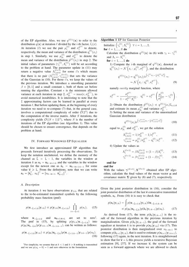
4

of the EP algorithm. Also, we use qp`qzipxq to refer to thedistribution qpxq at iteration ` divided by the i-th factor, tipxq.At iteration p`) we use the pair µp`qi and σ2p`q

i to denote,respectively, the mean and variance of the distribution qp`qi pxiqin step 1. Similarly, we use µ

p`qpi

and σ2p`qpi

to denote themean and variance of the distribution pp`qpxiq in step 2. Theinitial values of parameters pγp1qi ,Λ

p1qi q will be set according

to the problem at hand. The parameter update in (11) mayreturn a negative value Λ

p``1qi,new for some i’s which means

that there is no pair pΛp``1qi,new, γ

p``1qi,newq that sets the variance

of the Gaussian in (10). For those i’s, we keep the values ofthe previous iteration. We introduce a smoothing parameterβ P r0, 1s and a small constant ε, both of them set beforerunning the algorithm. Constant ε is the minimum allowedvariance at each iteration in step 2, σ2p`q

pi“ maxpε, σ2p`q

piq, to

avoid numerical instabilities. It is interesting to note that theI approximating factors can be learned in parallel at everyiteration `. But before updating them, at the beginning of everyiteration we need to re-compute (7) that, in the general case,involves a computational complexity of order OpI3q due tothe computation of the inverse matrix. After S iterations, thecomplexity yields OppS ` 1qI3q, where S is the number ofiterations of the EP algorithm (see Algorithm 1). This valueshould be chosen to ensure convergence, that depends on theproblem at hand.

IV. FORWARD WINDOWED EP EQUALIZER

We first introduce an approximated EP algorithm thatproceeds forward iteratively processing the observations. Tokeep the notation uncluttered, we define the memory of thechannel as L “ L ´ 1, the variables in the window atiteration k as sk “ uk´W`1:k and the variables in the windowexcept for the newest one as sk “ uk´W`1:k´1 for somevalue W ě L. From the definitions, note that we can writesk “ rsJk , uksJ “ ruk´W`1, sJk`1sJ.

A. Description

At iteration k we have observations y1:k, that are relatedto the to-be-estimated transmitted symbols by the followingprobability mass function (pmf):

ppu´L`1:k|y1:kq 9 ppy1:k|u´L`1:kqkź

i“´L`1

ppuiq, (15)

where u´L`1:0 and uN`1:N`L are set to zero1.The pmf in (15), by splitting ppy1:k|u´L`1:kq intoppyk|uk´L:kqppy1:k´1|u´L`1:k´1q, can be written as follows:

ppu´L`1:k|y1:kq 9 ppyk|uk´L:kqppu´L`1:k´1|y1:k´1qppukq.(16)

1For simplicity, we assume that at k ă 1 and k ą N nothing is transmittedand we use ppuk “ 0q “ 1 and zero otherwise in the formulation.

Algorithm 1 EP for Gaussian Posterior

Initialize´γp1qi ,Λ

p1qi

¯@ i “ 1, ..., I.

for ` “ 1, ..., S doCalculate the distribution qp`qpxq in (6) with γi Ð γ

p`qi

and Λi Ð Λp`qi .

for i “ 1, ..., I do1) Compute the i-th marginal of qp`qpxq, denoted asqp`qi pxiq “ N

´xi : µ

p`qi , σ2p`q

i

¯, and the distribution

qp`qzipxiq “ qp`qi pxiq{e

´γp`qi xi´ 1

2 Λp`qi x2

i

¯∼

∼ N´xi : η

p`qi , ν2p`q

i

¯, (9)

namely cavity marginal function, where

ν2p`qi “ σ2p`q

i

1´ σ2p`qi Λ

p`qi

, ηp`qi “ ν2p`q

i

˜µp`qi

σ2p`qi

´ γp`qi¸.

2) Obtain the distribution pp`qpxiq 9 qp`qzipxiqIxiPAand estimate its mean µp`qpi and variance σ2p`q

pi.

3) Setting the mean and variance of the unnormalizedGaussian distribution

qp`qzipxiqe´γp``1qi,newxi´ 1

2 Λp``1qi,newx

2i

¯(10)

equal to µp`qpi and σ2p`qpi

, we get the solution

Λp``1qi,new “ 1{σ2p`q

pi ´ 1{ν2p`qi , (11)

γp``1qi,new “ µ

p`qpi{σ2p`qpi ´ ηp`qi {ν2p`q

i . (12)

4) Update the values as

Λp``1qi “ βΛ

p``1qi,new ` p1´ βqΛp`qi , (13)

γp``1qi “ βγ

p``1qi,new ` p1´ βqγp`qi . (14)

end forend forWith the values γpS`1q,ΛpS`1q obtained after EP algo-rithm, calculate the final values of the mean vector µ andcovariance matrix Σ given by (8) and (7), respectively.

Given the joint posterior distribution in (16), consider thejoint posterior distribution of the last W consecutive transmittedsymbols, sk. From (16) it is easy to check that

ppsk|y1:kq “żppu´L`1:k|y1:kqdu´L`1:k´W

9 ppyk|uk´L:kqppsk|y1:k´1qppukq. (17)

As derived from (17), the term ppsk|y1:k´1q is the re-sult of the forward algorithm in the previous iteration bymarginalization. Given ppsk|y1:k´1q, the goal of the forwardequalizer at iteration k is to provide ppsk|y1:kq via (17). Thisposterior distribution is then marginalized over uk´W`1 tocompute ppsk`1|y1:kq, that is used to estimate ppsk`1|y1:k`1q,following (17) again, in the next iteration. It is straightforwardto show that for W “ L this process yields a recursive Bayesianestimation [9], [37]. If we increase W, the system can beseen as a forward approach where we are allowed to check

97

5

0 0 0

h3 h2 h1

0 u1

y1

u2

y2

u3

y3

uk

yk

. . .

uN´1

yN´1

. . .

uN

yN

0

yN`1

0

yN`2

0 0

qr1sf pr0, 0, 0, 0, u1sJq

qr2sf pr0, 0, 0, u1, u2sJq

qr3sf pr0, 0, u1, u2, u3sJq

qrN`3sf pruN´1, uN, 0, 0, 0sJq

qrN`4sf pruN, 0, 0, 0, 0sJq

Fig. 2: Factor graph associated to (1) for L “ 3, W “ 5 and FWEP performance.

for the W ´ L future observations, improving the estimationsfor the first symbols in the window. The main advantage ofthe whole procedure is that the complexity is linear with thenumber of iterations. However, marginalizing (17) to computeppsk`1|y1:kq has complexity OpMWq, that increases rapidlywith the length of the window W, and/or the size of theconstellation, M. At this point we rely on an EP-based Gaussianapproximation to (17). First, we rewrite the term ppsk|y1:k´1qin (17) as follows

ppsk|y1:k´1q 9 ppy1:k´1|skqk´1ź

i“k´W`1

ppuiq (18)

and introduce it into (17), yielding

ppsk|y1:kq 9 ppyk|uk´L:kqppy1:k´1|skqkź

i“k´W`1

ppuiq. (19)

This expression is appealing, since it fits the model (5) forwhich an EP approximation is described. Assume for nowthat the previous EP forward iteration provided a Gaussianapproximation to ppy1:k´1|skq, that we denote by grk´1spskq.We propose to use the following family F of Gaussian pdfsto find an EP-based approximation to (19)

qrksf pskq def“ ppyk|uk´L:kqgrk´1spskq

kź

i“k´W`1

e

´γrksi ui´ 1

2 Λrksi u2

i

¯.

(20)

We use the superscript rks to explicitly indicate at what itera-tion the different terms are updated. For instance, grk´1spskqwas computed at iteration k´1, while qrksf pskq, γrksi and Λ

rksi

were computed at iteration k. Also, the subscript f in qrksf pskqis included to avoid confusion with the equivalent estimationprovided by the backward counterpart of the algorithm ex-plained in Section V. Note that qrksf pskq in (20) is a functionof parameters γrksi and Λ

rksi for i “ k ´ W ` 1, ..., k. Details

about how to compute these parameters with EP to ensure that(20) has mean and covariance matrix close to those in (19) aregiven in the next subsection. After the EP approximation in(20) has been computed, we can easily estimate the marginalover the symbol uk´W`1, namely q

rksf puk´W`1q, which is fed

to the channel decoder. Also, recall that sk “ ruk´W`1, sk`1sand thus after integrating out uk´W`1 in (20) we obtain

qrksf psk`1q, the current EP approach to ppsk`1|y1:kq. Finally,

the k-th iteration of the forward windowed EP equalizer endsby computing the moments of the Gaussian distribution

grkspsk`1q “qrksf psk`1q

kśi“k´W`2

e

´γrksi ui´ 1

2 Λrksi u2

i

¯ , (21)

which by (18) is the current approximation to ppy1:k|sk`1qand will be used in the next iteration of the forward windowedEP equalizer. Table I summarizes the distributions defined todescribe each iteration of the algorithm.

TABLE I: Gaussian distributions in the FWEP equalizer.

Distribution Approximates Mean Cov. Matrixgrk´1spskq ppy1:k´1|skq µg,rk´1s Σg,rk´1s

qrksf pskq ppsk|y1:kq µq,rks Σq,rks

qrksf psk`1q ppsk`1|y1:kq µ

q,rksz1 Σ

q,rksz1,z1

grkspsk`1q ppy1:k|sk`1q µg,rks Σg,rks

In the following, to keep the notation uncluttered, we willrefer to γrksi and Λ

rksi simply as γi and Λi. In Fig. 2 we depict

the factor graph associated to (1) for the case L “ 3 and W “ 5where the sliding window is drawn with dashed lines. It can beobserved that in each iteration the window is moved forward,including a new transmitted symbol and a new observation,and marginalizing over the oldest transmitted symbol. Asa result, we have a linear complexity with the number ofiterations, N, and cubic complexity with the window length,W. We denote this method as forward windowed expectationpropagation (FWEP).

B. Formulation

In the development of the FWEP algorithm we assumethat the initial and final transmitted symbols are known.In particular, and without loss of generality, u´W`2:0 areassumed zero. Hence, the pmf for sk at the first iteration,k “ 1, is pps1 “ r0...0sJq “ 1 and zero otherwise.This pmf is approximated in the EP approach by definingGaussians with zero mean and a low enough variance, i.e.,


6

qr0sf ps1q “ N

`s1 : r0 . . . 0sJ, σ2

minI˘. In a similar way, recall

that for the last k “ N` 1, ..., N` W´ 1 iterations we assumethat the final transmitted symbols uN`1:N`W´1 are zero. Forthese symbols, we force pγk,Λkq “ p0, σ´2

minq and keep themfixed.

In the following, we present the formulation of the FWEPupdate rules focusing on learning the approximated distri-butions in (20) and (21). We assume that, as a result ofthe previous FWEP iteration, the moments of grk´1spskq, i.e.µg,rk´1s and Σg,rk´1s are known. The Gaussian likelihoodfactor ppyk|uk´L:kq in (19) is given by the channel model in(1). If we define Q “ σ´2

w hL:1hJL:1 and r “ σ´2

w hL:1yk, itis possible to merge the first two terms in (20) into just oneGaussian distribution and rewrite it as

qrksf pskq def“ N

´sk : zrks,Crks

¯ kź

i“k´W`1

epγiui´ 12 Λiu

2i q (22)

where

Crks´1 “

“„0pW´LqˆpW´Lq 0pW´LqˆL

0LˆpW´Lq Q

`«´

Σg,rk´1s¯´1

0pW´1qˆ1

01ˆpW´1q 0

ff,

(23)

Crks´1

zrks “˜„

0pW´Lqˆ1

r

`«´

Σg,rk´1s¯´1

µg,rk´1s

0

ff¸.

(24)

Note that the goal of the EP approximation at iteration k isto find Λk´W`1:k and γk´W`1:k in (22) so that the momentsof qrksf pskq approximate well the moments of ppsk|y1:kq in(19). Further, note that the model in (22) is equivalent to thatdescribed in Subsection III-A and thus to learn Λk´W`1:k andγk´W`1:k we can resort directly to Algorithm 1. Parameterspγi,Λiq @i P rk´W`1, k´1s are initialized to the values ob-tained in the previous k-th iteration while pγk,Λkq “ p0, Esq.The mean and covariance of the resulting pdf for qrksf pskq,N

`sk : µq,rks,Σq,rks˘, are given by (8) and (7),

Σq,rks “´Crks

´1 ` diagpΛk´W`1:kq¯´1

, (25)

µq,rks “ Σqrks´Crks

´1zrks ` γk´W`1:k

¯. (26)

Finally, given Σq,rks and µq,rks, the moments of grkspsk`1qare straightforward to compute. From (21) we obtain:

´Σg,rks

¯´1 “´Σq,rksz1,z1

¯´1 ´ diagpΛk´W`2:kq (27)

µg,rks “ Σg,rksˆ´

Σq,rksz1,z1

¯´1

µq,rksz1 ´ γk´W`2:k

˙, (28)

where µq,rksz1 is the vector µq,rks in (26) without the first

element and Σq,rksz1,z1 is the submatrix obtained by removing

from Σq,rks in (25) the first row and column. A detailedimplementation of the FWEP iterative algorithm is included inAlgorithm 2. Since we use a window of size W, the transmittedsymbol uk is involved in W iterations, i.e., from iteration k to

Algorithm 2 The FWEP approximationSet the value of the parameter W.Initialize Σq,r0s “ diagpσ2

minr1 ¨ ¨ ¨ 1sq, µq,r0s “ r0 ¨ ¨ ¨ 0sJ,γ´W`2:0 “ r0 ¨ ¨ ¨ 0sJ and Λ´W`2:0 “ σ´2

minr1 ¨ ¨ ¨ 1sJ.for k “ 1, ..., N` W´ 1 do

1) Initialize Algorithm 1 with

pγk,Λkq “#p0, E´1

s q if 1 ď k ď N

p0, σ´2minq if N ă k ď N` W´ 1

(29)

and pγi,Λiq for i P rk ´ W ` 1, k ´ 1s with the valuesobtained in the previous k-th iteration.2) Apply Algorithm 1 with S, I “ N, x “ sk “uk´W`1:k, and z and C in (6) given by (24) and (23),respectively. Any estimate pγi,Λiq with i P r´W ` 2, 0sor i P rN` 1, N` W´ 1s is not updated.

end for

k`W´1, and we have W different estimations for each symbol.We use the approximation q

rk`W´1sf psk`W´1q to estimate uk

since it is the one that includes more observations, specificallyit exploits the received observations until time k` W´ 1, i.e.,y1:k`W´1. At every iteration, k, the computational complexityof the FWEP is dominated by the inversion of the covari-ance matrix in (25), of dimension W. Therefore, we have aquite efficient implementation with computational complexityOppS ` 1qNW3q, where S is the number of iterations of the EPalgorithm. Note that after the EP algorithm, a last inversionis needed to compute the APP. A lower value for W reducesthe computational complexity, however a larger size involvesmore future observations and improves the estimation. A valueW ě L, implies that all observations directly connected to theto be-estimated variable are included. Note that W “ L definesthe state for the recursive Bayesian estimator.

V. BACKWARD WINDOWED EXPECTATION PROPAGATION

As already discussed, the approximation used for FWEPexploits the received observations until time k ` W ´ 1, i.e.,y1:k`W´1 to estimate uk. However, it does not use the informa-tion of the following ones, yk`W:N`W´1. We next propose thebackward recursion as a first step to include these observationsin the estimation. The key idea is just to use the sameformulation for the FWEP but from the end of the sequenceof observations towards the begining. This algorithm can beeasily formulated by left-right flipping the channel, observa-tion and symbol vectors, and applying the FWEP algorithm tothem, as illustrated in Fig. 3. We denote this method backwardwindowed expectation propagation (BWEP). In Fig. 3 weinclude the factor graph in Fig. 2 flipped. The FWEP is appliedto this graph to get the BWEP solution. In Appendix A wedescribe the change of variables associated to this flippingneeded to run the BWEP algorithm as an instance of theFWEP. Note that there is an L´1 offset in the relative positionof the observations, yk, and transmitted symbols, uk, withrespect to Fig. 2. This way we ensure that, at each iteration k,the sliding window is shifted to include a new observation yk,and all its directly connected symbols, uk´L`1:k. As a result,

99

7

0 0 0

h1 h2 h3

0 uN

yN`2

uN´1

yN`1

uN´2

yN

uk

yk`2

. . .

u2

y4

. . .

u1

y3

0

y2

0

y1

0 0

qrN`4sb pr0, 0, 0, 0, uNsJq

qrN`3sb pr0, 0, 0, uN, uN´1sJq

qrN`2sb pr0, 0, uN, uN´1, uN´2sJq

qr2sb pru2, u1, 0, 0, 0sJq

qr1sb pru1, 0, 0, 0, 0sJq

Fig. 3: Factor graph associated to (1) for L “ 3, W “ 5 and BWEP performance. The sliding window, dashed, shifts from leftto right.

the BWEP will provide a Gaussian approximation, qrksb pskq,to ppsk|yk´W`L:N`W´1q, k “ 1, ..., N ` W ´ 1, from which weestimate by marginalization a pmf for the symbol uk (recallthat in the FWEP case, we marginalize qrksf pskq to estimatesymbol uk´W`1).

VI. SMOOTHED EXPECTATION PROPAGATION

The estimation in the FWEP ignores the future observationswhile the BWEP estimation does not exploit the previousones. In this section we introduce the smoothing expectationpropagation (SEP) to improve the estimation by mergingboth procedures into one. In the forward bayesian recursiveapproach, the optimal solution can be estimated with a windowsize of L. This window size can be adopted for the FWEP, toestimate the posterior of uk from uk:k`L. Following the samereasoning, to estimate the posterior of uk with the BWEP wewould use a window of L spanning uk´L:k. In order to dealwith both estimations, we implement both algorithms witha window size 2L ´ 1 and combine their estimates. In thefollowing we show how both estimations can be merged anddescribe the SEP algorithm.

A. Description

As in the forward approach, we first rewrite the wantedprobabilities into a suitable form for the EP algorithm. Thefollowing lemma summarizes this first result.

Lemma 6.1: The posterior probabilites, ppuk´L:k`L|yq, upto a constant, can be written as

ppuk´L:k`L|yq 9ppuk´L:k`L|y1:k`Lqppuk´L:k`L|yk:N`Lq

k`Lśi“k

ppyi|ui´L:iqk`Lśi“k´L

ppuiq.

(30)

Proof: From (2), the exact posterior probability distribu-tion is

ppu|yq 9 ppy|uqppuq “N`Lź

k“1

ppyk|uk´L:kqN`Lź

k“´L`1

ppukq(31)

where u´L`1:0 and uN`1:N`L are known. We aim at esti-mating uk, by using q

rk`Lsf psk`Lq in the forward step and

qrk`Lsb psk`Lq in the backward step. Accordingly, we split (31)

in two parts: received symbols until time k` L and after timek ` L,

ppu|yq “ 1

ppyqppy1:k`L|u´L`1:k`Lqppu´L`1:k`LqN`Lź

i“k`L`1

ppyi|ui´L:iqppuiq

9 ppu´L`1:k`L|y1:k`LqN`Lź

i“k`L`1

ppyi|ui´L:iqppuiq. (32)

We now marginalize ppu|yq over u´L`1:k´L´1 simplifying thefirst factor, from the FWEP description in (17),

ppuk´L:N`L|yq 9 ppuk´L:k`L|y1:k`LqN`Lź

i“k`Lppyi|ui´L:iqppuiq.

(33)

To rewrite the last term of (33) into the posteriorppuk´L:N`L|yk:N`Lq, the following factors are missing

k`Lź

i“kppyi|ui´L:iq

k`Lź

i“k´Lppuiq. (34)

By multiplying and dividing (33) by (34), we get the equiv-alent distribution

ppuk´L:N`L|yq 9ppuk´L:k`L|y1:k`Lqppuk´L:N`L|yk:N`Lq

k`Lśi“k


ppuiq.

(35)

Then after marginalizing ppuk´L:N`L|yq over the last symbolsuk`L:N`L, it yields (30).

Assume we run the FWEP and BWEP algorithms with W “2L´1. Note that with this window size sk`L “ uk´L:k`L. Wepropose to approximate the numerator in (30) by using theforward and backward approximations developed in SectionsIV and V as follows,

ppuk´L:k`L|y1:k`Lq Ñ qrk`Lsf psk`Lq (36)

ppuk´L:k`L|yk:N`Lq Ñ qrk`Lsb psk`Lq, (37)


8

whereÑ denotes that the term on its left is replaced by the oneto its right. Regarding the priors in the denominator of (30),we approximate them by exponentials as we did in (5)-(6),

k`Lź

i“k´Lppuiq Ñ

k`Lź

i“k´Lepγiui´ 1

2 Λiu2i q. (38)

We assign to the pairs pγi,Λiq the values obtained with thek ` L forward approximation for k ă i ď k ` L (denotedas γf k`1:k`L, Λf k`1:k`L) and with the k ` L backwardapproximation for k ´ L ď i ď k (denoted as γbk´L:k,Λbk´L:k). The SEP approximation yields

ppsk`L|yq «qrk`Lsf psk`Lqqrk`Lsb psk`Lq

k`Lśi“k


epγiui´ 12 Λiu2

i q, (39)

where the r.h.s. is already a Gaussian distribution and, thus,there is no need for further EP approximations. First, the twofactors in the numerator are Gaussian distributions computedby the FWEP/BWEP algorithms:

qrk`Lsf psk`Lq “ N

´sk`L : µ

q,rk`Lsf ,Σ

q,rk`Lsf

¯, (40)

qrk`Lsb psk`Lq “ N

´sk`L : µ

q,rk`Lsb ,Σ

q,rk`Lsb

¯. (41)

Using the Gaussian channel likelihood, it is straightforwardto show that the r.h.s. of (39) is a Gaussian distribution withcovariance matrix

pΣfbq´1 “´Σq,rk`Lsf

¯´1 `´Σq,rk`Lsb

¯´1

´ σ´2w HJ

L HL ´ diagpΛfbq, (42)

and mean

µfb “ Σfb

„´Σq,rk`Lsf

¯´1

µq,rk`Lsf `

´Σq,rk`Lsb

¯´1

µq,rk`Lsb

´ `σ´2w HJ

L yk:k`L ` γfb

˘‰, (43)

where HL is a Lˆp2L´ 1q matrix formed by the L first rowsof a circulant matrix with first row rhL:1

J,01ˆLs and

Λfb “„

Λbk´L:kΛf k`1:k`L

, γfb “

„γbk´L:kγf k`1:k`L

. (44)

Using the obtained Gaussian approximation to ppsk`L|yq,we marginalize to obtain a probabilistic estimation to theposterior probability of the uk symbol. The main steps ofthe SEP iterative algorithm are summarized in Algorithm 3.Since the SEP algorithm needs the forward and backwardapproximations computed by FWEP and BWEP, its finalcomplexity is dominated by the computational cost of thesealgorithms, i.e., OpNpS ` 1qp2L´ 1q3q.

B. Windowed Linear MMSE and SEP turbo equalization

In the light of this result, it is interesting to point out that awindowed linear (recursive) MMSE can be easily derived fromthe formulation of the SEP by just running the SEP algorithmwithout entering in the EP iterative loop, i.e., forcing S “0. We will denote this approach, the SEP with S “ 0, as

Algorithm 3 The SEP estimator1) Compute forward approximations with the FWEP algo-rithm detailed in Algorithm 2 with W “ 2L` 1.2) Compute backward approximations using Algorithm 2 asdescribed in Section V with W “ 2L` 1.for k “ 1, ..., N do

Compute (42) and (43) and marginalize to estimate theAPP ppuk|yq.

end for

WLMMSE. Note that if no iterations of EP are performed wehave γrksi “ γ

rk´1si and Λ

rksi “ Λ

rk´1si . Accordingly, (20) can

be reduced to

qrksf pskq “ ppyk|uk´L:kqqrk´1s

f pskqepγkuk´ 12 Λku

2kq, (45)

where we removed the superindexes of γk and Λk. Thisexpression, up to a constant, equals (17) particularized tothe scenario where ppukq is given and assumed to be Gaus-sian distributed, ppukq9 exp

`γkuk ´ 1

2Λku2k

˘, and we have a

Gaussian likelihood that can be easily computed, qrk´1sf pskq “

ppsk|y1:k´1q. Therefore, in this scenario the FWEP withS “ 0 is a Kalman filtering and the SEP yields the smoothingversion.

The performance of soft-output equalizers can be improvedby using a turbo equalization approach [7], [19], [38]. Theextrinsic information at the output of the decoder, LDpbtq,after mapping, pDpukq, is handed back to the SEP equalizer.Then pDpukq is approximated by a Gaussian whose mean andvariance are used to initialize the EP parameters, pγp1qi ,Λ

p1qi q,

in Algorithm 1, when called in Algorithm 2. The extrinsicinformation handed to the decoder consists in the cavityfunctions (see Algorithm 1) at the end of the SEP algorithm,once demapped. This process can be repeated T times or untilconvergence.

TABLE II: Complexity comparison between algorithms.

Algorithm Complexity

SEP NpS ` 1qp2L´ 1q3BEP pS ` 1qLN2

WLMMSE NW2

BCJR NML

Approx. BCJR NMeM

C. Computational Complexity

In Table II we include a detailed comparison of the com-plexity of the SEP, the algorithm in [31] (BEP), WLMMSE,BCJR, and approximated approaches, where Me is the numberof survivor states and W depends linearly with L. As M

and/or L grow, the BCJR and approximate approaches becomecomputationally unaffordable. Due to the quadratic complexityof BEP in the frame length, the only feasible solutions for largeN are the SEP and the WLMMSE, where the performance ofthe SEP quite outperforms that of the WLMMSE, as illustratedin the next section.

101

9

8 10 12 14 16 18 20

10´4

10´3

10´2

10´1

Eb{N0 (dB)

BER

LMMSE

WLMMSE

SEP

FWEP

BWEP

AWGN

Fig. 4: BER for 64-QAM and 10 random channels with L “ 7.

VII. EXPERIMENTAL RESULTS

In this section, we illustrate the good performance of theSEP equalizer for different scenarios. We use a regular LDPCof rate 1/2, with a maximum number of 200 iterations at thedecoder. The codes used in this paper are (3,6)-regular LDPCgenerated using the progressive-edge growth (PEG) algorithm[39], and the belief propagation was used as channel decoder[40], [41]. The PEG algorithm ensures the largest possiblegirth according to the design parameters, i.e. the block lengthN and the degree distribution. We limit to 5 the maximumabsolute value of the LLR at its input in order to avoid veryconfident probabilities which negatively affect the decoder.We average the BER over 1000 different frames per channelrealization. When random channels are used, each tap is i.i.d.Gaussian distributed, circular when complex, with zero meanand equal variance, 1{L. The channel response is normalized.In all experiments in this paper we set W “ 2L ´ 1, β “ 0.1,ε “ 0.5 and σ2

min “ 1e´3. S “ 10 except for the case afterthe turbo procedure has started, where S “ 1. These valueswere selected after extensive experimentation as a trade offbetween convergence speed and accuracy. In the BER curves,we include the block implementation of the LMMSE algorithmas reference. We also show the WLMMSE performance in thefirst figures to illustrate that it exhibits the same performanceas the block implementation. For low complexity scenarios,the BCJR and its approximated solutions, the M-BCJR [11],M*-BCJR [14], RS-BCJR [10], NZ and NZ-OS [12] ap-proaches are also included. The AWGN bound is also addedin some of the figures as reference.

A. FWEP and BWEP

In Fig. 4 we illustrate the performance of the FWEP andthe BWEP for T “ 0. We depict the BER average formi, see Fig. 1, over 10 random complex-valued channelsfor L “ 7, a 64-QAM modulation and codewords of 4098bits. We also include the performance of the SEP, mergingthe estimation from both the FWEP and BWEP approaches,i.e. exploiting the whole vector of observations. Note thatthe LMMSE/WLMMSE need the whole observation vector

5.5 6 6.5 7 7.5 810´5

10´4

10´3

10´2

10´1

Eb{N0 (dB)

BER

LMMSE

WLMMSE

SEP

BCJR

M-BCJR

M*-BCJR

RS-BCJR

NZ

NZ-OS

Fig. 5: BER for BPSK and a specific minimum phase channelh “ 1?

140r7 6 5 4 3 2 1sJ.

to achieve a similar performance to the one of the FWEP (orthe BWEP).

B. Low complexity scenario

In Fig. 5 and Fig. 6 we study the performance for typicalchannels used in the literature [12] to compare approximationsto the BCJR algorithm. We use codewords of block length1024 bits. In Fig. 5 we consider the minimum phase channel,h “ 1?

140r7 6 5 4 3 2 1sJ and BPSK symbols. The BCJR has

64 states per step, while its approximations are computed withMe “ 4 states, as described in [12]2. In Fig. 6 we simulatethe maximum phase channel h “ 1?

140r1 2 3 4 5 6 7sJ and

BPSK symbols. Now, we use Me “ 8 states as in [12] forthe approximated solutions. In Fig. 7 and Fig. 8 we averagethe BER over 100 random channels with 5 real-valued taps.We set the number of states for the approximated solutionsto Me “ 8. In Fig. 7, we consider BPSK modulation, theBCJR has 16 states per step, while in Fig. 8 a 4-PAM is used,increasing the number of states to 256 in the BCJR algorithm.

In view of these results we may conclude that many algo-rithms approximating the optimal solution in the literature arequite dependent on the channel realization. Not only becausethey are based in just a forward or a backward strategy, butalso because the parameters for some approximations need tobe tuned for the particular channel. In this sense, the approxi-mations M-BCJR, M*-BCJR and RS-BCJR fail, as observedin Fig. 6. On the other hand, we analyze how approximationsbased on tracking just a subset of paths or states, Me, behaveas the number of states grows. If the number of subsets, Me, iskept as a fraction of the total number, they may exhibit a goodperformance. But if a large number of states is unaffordable, afraction of it is also intractable. In the first cases, Fig. 5, Fig. 6and Fig. 7, both NZ and NZ-OS algorithms have quite goodperformance because the state reduction ratio (ML{Me) is low.However, when we increase the number of states keeping the

2The number of states in approximated solutions are chosen according tothe ones in [12]. We run FT, BT or DT depending on the phase of the channeland denote all of them in the results by NZ (and NZ-OS).


10

5 5.5 6 6.5 7 7.5 810´5

10´4

10´3

10´2

10´1

Eb{N0 (dB)

BER

LMMSE

WLMMSE

SEP

BCJR

M-BCJR

M*-BCJR

RS-BCJR

NZ

NZ-OS

Fig. 6: BER for BPSK and a specific maximum phase channelh “ 1?

140r1 2 3 4 5 6 7sJ.

2 4 6 8 1010´5

10´4

10´3

10´2

10´1

Eb{N0 (dB)

BER

LMMSE

SEP

BCJR

M-BCJR

M*-BCJR

RS-BCJR

NZ

NZ-OS

AWGN

Fig. 7: BER for BPSK and 100 random channels with L “ 5.

number Me fixed, the solution degrades, as can be observedin Fig. 8. The performance of the SEP is close to the one ofthe BCJR, within 0.75-2 dB in the four scenarios, regardlessof the channel. The LMMSE also exhibits a robust behavior,but it quite deviates as the number of states grows. Note thatthe BCJR algorithm is computationally affordable in thesescenarios, but its complexity increases exponentially with thedimension of the scenario, similarly to its approximations. Outof the approaches compared in these experiments, just theSEP and the LMMSE soft equalizers are available for largeconstellations. In the following, we study their performance.

C. Large complexity scenario

In Fig. 9, we depict the BER curves after the LDPC decoderfor SEP, BEP [31] and LMMSE soft equalization, consideringcodewords of 4096 bits, channels of L “ 7 complex-valuedtaps with 16-QAM modulation (solid lines) and 64-QAMmodulation (dashed lines). By including the BEP approach,we show that the SEP approach reduces the complexity of ourprevious work, with no degradation in the performance. TheSEP exhibits a good performance compared to the LMMSE.

5 10 1510´5

10´4

10´3

10´2

10´1

Eb{N0 (dB)

BER

LMMSE

SEP

BCJR

M-BCJR

M*-BCJR

RS-BCJR

NZ

NZ-OS

AWGN

Fig. 8: BER for 4-PAM and 100 random channels with L “ 5.

5 10 15 20 2510´5

10´4

10´3

10´2

10´1

Eb{N0 (dB)

BER

LMMSE

SEP

BEP

AWGN

Fig. 9: BER after the channel decoder for 16-QAM (solid lines)and 64-QAM (dashed lines), 500 random channels with L “ 7 andcodewords of 4096 bits.

For 16-QAM we have a gain of 3 dB, while for 64-QAM weimprove it in 5 dB.

D. Performance analysis

We compare probabilistic equalizers using a information-theoretical metric: the mutual information between the trans-mitted symbol uk and uk, which is a random variable dis-tributed according to the estimation to the posterior distributionof uk given y (the observation for the whole sequence):

Ipuk, ukq “ÿ

uk

ÿ

uk

ppuk, ukq log2

ppuk|ukqppukq , (46)

where note that ppuk, ukq is the joint probability distributionof uk and uk after marginalizing the channel output y, thechannel impulse response (in the case we consider it random)and the rest of symbols in the sequence u. As the aboveexpression cannot be evaluated in closed-form, we resort toMonte Carlo estimates to generate samples from ppuk, ukq andthen evaluate Ipuk, ukq from these samples. Assume that thechannel taps are Gaussian distributed, but are perfectly knownat the receiver. First, we collect N P Z` samples from the joint

103

11

0 5 10 15 20 25

2

4

6

Eb{N0 (dB)

Ipu

k,u

kq

SEPLMMSE

10 12 143

3.5

4

4.5

5

Fig. 10: Mutual information for SEP and LMMSE for 64-QAM andrandom channels with L “ 7.

distribution of u,h,y and uk using ancestral sampling [36].Each sample of the joint distribution is obtained as follows:

1) Sample u from a uniform distribution in the constellation.2) Sample the channel coefficients h.3) Sample y according to ppy|u,hq.4) Sample uk according to ppuk|yq.

Second, after N samples of possible puk, ukq pairs have beencollected, we use these samples to estimate ppukq, ppuk|ukqand, finally, Ipuk, ukq in (46). It is important to observe thatppuk|yq is dependent on the probabilistic detection methodconsidered. The higher Ipuk, ukq is for each probabilisticequalizer, the closer we perform to channel capacity. InFig. 10 we depict the mutual information in (46) computedfor N “ 106 samples per Eb{N0 point and averaged overall the symbols in the transmitted sequence, for the SEP andLMMSE algorithms, considering a 64-QAM constellation andchannels of L “ 7 complex-valued taps. A magnification forintermediate Eb{N0 is shown in the upper left corner. Observethat, for very small Eb{N0, the noise is so large that bothmethods achieve a small mutual information. On the otherhand, for very large Eb{N0 values, both methods converge to6 bits, i.e., the number of bits transmitted per QAM symbol.Any probabilistic method will eventually saturate to this value.However, the key aspect is to be able to design a probabilisticequalizer able to improve the mutual information for interme-diate Eb{N0 values. Observe that before the saturation, theSEP achieves a gain w.r.t. LMMSE of around 2 dB.

E. EXIT Charts and Turbo Equalization

The performance of the SEP equalization and turbo equali-zation can be analyzed with extrinsic information transfer(EXIT) charts [19], [42], [43]. The EXIT charts for theequalizer represent the improvement of the mutual informationbetween the estimation at the output and the true symbols.By also including the EXIT chart of the channel decoder,we can predict the evolution of the interchange of extrinsicinformation from the equalizer to the channel decoder andback to the equalizer in turbo equalization.

0 0.2 0.4 0.6 0.8 10

0.2

0.4

0.6

0.8

1

IiI o

SEP, Eb/No=6 dB

LMMSE, Eb/No=6 dB

SEP, Eb/No=4 dB

LMMSE, Eb/No=4 dBLDPC Decoder

Fig. 11: EXIT charts for the decoder, the SEP and LMMSEequalizers with 4 and 6 dB of Eb{No. BPSK modulation was used.

In Fig. 11 we include the EXIT charts of the SEP (˝)and LMMSE (˝) equalizers for the channel response h “r0.227 0.46 0.688 0.46 0.227sJ [19], BPSK transmission andEb{No “ 6 (solid) and 4 dB (dashed). The EXIT chart of theLDPC decoder with N “ 1024 used is also depicted (solid).The horizontal axis is the mutual information of the LLR at theinput, Ii. The vertical axis is the same measure for the output,Io. The evolution of the mutual information for Eb{No “ 4dB along iterations of the SEP and LMMSE turbo equalizationare indicated with arrows. An arrow is included each time theequalizer (vertical arrow) or the channel decoder (horizontalarrow) is run. Note that Io at the output of the equalizer is alsothe value at the input of the channel decoder. In the figure, itis shown that the trajectory of the SEP turbo approach is ableto successfully equalize and decode. In the LMMSE, at thesecond iteration of the turbo scheme the trajectory gets stuck,at Ii « 0.1, where the curve of the LMMSE intersects thecurve of the channel decoder. Since the EXIT chart for theSEP and Eb{No “ 4 dB is close to the one of the LMMSEfor Eb{No “ 6 dB, a 2 dB gain is expected in this scenario.

In Fig. 12 we depict the BER curves after the LDPC decoderfor SEP turbo equalization, considering channels of L “ 7complex-valued taps, 64-QAM modulation and codewords ofN “ 1024 bits. The number of EP iterations once the turboprocedure starts is set to S “ 2. Due to the iterative procedureof the feedback scheme, we reduced the maximum number ofiterations in the LDPC decoder to 100. We represent the first2 iterations and fifth iteration of the turbo scheme. It canbe observed that the SEP without turbo already finds a verygood estimate, still outperforming in 1.75 dB at a BER of10´4 the performance of the LMMSE turbo equalizer after 5loops. Therefore, the SEP receiver brings a remarkable gainin performance, but also a drastic latency reduction, sinceno feedback loop is required at least to improve the turbo-LMMSE scheme. In any case, if SEP is incorporated into theturbo receiver, we obtain an extra gain of about 0.75 dB afterthe first turbo iteration, which can be improved in 0.25 dB in


12

16 18 20 22 2410´5

10´4

10´3

10´2

10´1

Eb{N0 (dB)

BER

SEP

LMMSE

Fig. 12: BER for SEP (green lines, solid) and LMMSE (blue lines,dashed) using the feedback loop for 64-QAM, 500 random channelswith L “ 7 and codewords of v “ 4096 bits. No feedback (˝), oneloop (Ÿ), two loops (˝) and five loops (`).

successive turbo iterations.

VIII. CONCLUSION

In large dimension scenarios, optimal turbo and soft channelequalization become intractable. In particular, large constella-tions cannot be addressed with the BCJR solution or theirapproximations. They need to compute and store a hugenumber of states, and the performance of the approximations isquite dependent on the channel realizations. Classical methodssuch as LMMSE equalization can be used as an affordablealternative, with poorer performance. Its performance can beimproved with turbo equalization. The complexity is linear inN and quadratic in the length of the window used. It can bereduced by using approximations.

In this paper, we propose the SEP as novel EP based softequalizer with the following advantages. Firstly, the order ofits computational complexity is linear with the frame length, N.Secondly, this new solution outperforms the LMMSE equal-izer in terms of BER. Finally, based on the results of theexperiments included, we get improvements with respect to theLMMSE in the range 2-5 dB exhibiting a good performanceregardless of the channel response.

APPENDIX ABACKWARD WINDOWED EP EQUALIZER

In this appendix we introduce the change of variables thatallows to run the BWEP algorithm as a particular instance ofFWEP. Define

uÐi “ uN`1´i i “ ´W` 2, ..., N` W´ 1 (47)sÐk “ uÐk´W`1:k k “ 1, ..., N` W´ 1 (48)yÐk “ yN`W´L`1´k k “ 1, ..., N` W´ 1 (49)hÐl “ hL`1´l l “ 1, ..., L. (50)

These definitions have been proposed to allow using (20).We obtain the backward approximated distribution for k “

1, ..., N ` W ´ 1, by applying the FWEP with the vectors in(47)-(50),

q1rksb psÐk q def“ qrksf psÐk q “

“ ppyÐk |uÐk´L:kqgrk´1spsÐk qkź

i“k´W`1

epγiuÐi ´ 12 Λiu

Ði

2q. (51)

To later ease the combination of the forward and backwardalgorithms we propose to change the indexing, and defineqrksb pskq def“ q1rN`W´ksb psÐN`W´kq. By using this change of

variable in the superscript, in the first iteration we estimateqrN`W´1sb puN`W´1:Nq while in the last one q

r1sb pu1:´W`2q, as

described in Fig. 3.

REFERENCES

[1] R. Schober, “Detection and estimation of signals in noise,” Universityof British Columbia, Vancouver, Tech. Rep., 2010.

[2] J. G. Proakis, Digital Communications, 5th ed. New York, NY:McGraw-Hill, 2008.





[7] M. Tuchler and A. Singer, “Turbo equalization: An overview,” IEEETrans. on Information Theory, vol. 57, no. 2, pp. 920–952, Feb 2011.


[9] F. Kschischang, B. Frey, and H.-A. Loeliger, “Factor graphs and thesum-product algorithm,” IEEE Trans. on Information Theory, vol. 47,no. 2, pp. 498 –519, Feb 2001.

[10] G. Colavolpe, G. Ferrari, and R. Raheli, “Reduced-state BCJR-typealgorithms,” IEEE Journal on Sel. Areas in Communications, vol. 19,no. 5, pp. 848–859, May 2001.



[13] C. Vithanage, C. Andrieu, and R. Piechocki, “Approximate inferencein hidden Markov models using iterative active state selection,” IEEESignal Processing Letters, vol. 13, no. 2, pp. 65–68, Feb 2006.


[15] M. Eyuboglu and S. Qureshi, “Reduced-state sequence estimation withset partitioning and decision feedback,” IEEE Trans. on Communica-tions, vol. 36, no. 1, pp. 13–20, Jan 1988.

[16] A. Duel-Hallen and C. Heegard, “Delayed decision-feedback sequenceestimation,” IEEE Trans. on Communications, vol. 37, no. 5, pp. 428–436, May 1989.

[17] P. Chevillat and E. Eleftheriou, “Decoding of trellis-encoded signals inthe presence of intersymbol interference and noise,” IEEE Trans. onCommunications, vol. 37, no. 7, pp. 669–676, Jul 1989.

[18] K. Muranov, “Survey of MMSE channel equalizers,” University ofIllinois, Chicago, Tech. Rep.


[20] M. Tuchler, A. Singer, and R. Koetter, “Minimum mean squarederror equalization using a priori information,” IEEE Trans. on SignalProcessing, vol. 50, no. 3, pp. 673–683, Mar 2002.

[21] R. Drost and A. Singer, “Factor-graph algorithms for equalization,” IEEETrans. on Signal Processing, vol. 55, no. 5, pp. 2052–2065, May 2007.

105

13

[22] L. Liu and L. Ping, “An extending window MMSE turbo equalizationalgorithm,” IEEE Signal Processing Letters, vol. 11, no. 11, pp. 891–894, Nov 2004.










[32] R. R. Lopes and J. R. Barry, “The soft-feedback equalizer for turboequalization of highly dispersive channels,” IEEE Trans. on Communi-cations, vol. 54, no. 5, pp. 783–788, May 2006.

[33] J. Jiang, C. He, E. M. Kurtas, and K. R. Narayanan, “Performance ofsoft feedback equalization over magnetic recording channels,” in Proc.IEEE International Magnetics Conference (INTERMAG), May 2006, p.795.

[34] J. Tao, “On low-complexity soft-input soft-output decision-feedbackequalizers,” IEEE Communications Letters, vol. 20, no. 9, pp. 1737–1740, Sep 2016.



[37] S. Haykin, Adaptive Filter Theory, 4th ed. Upper Saddle River, NJ,USA: Prentice-Hall, Inc., 2002.


[39] X.-Y. Hu, E. Eleftheriou, and D. M. Arnold, “Regular and irregularprogressive edge-growth tanner graphs,” IEEE Trans. on InformationTheory, vol. 51, no. 1, pp. 386–398, 2005.

[40] T. J. Richardson and R. Urbanke, Modern Coding Theory. CambridgeUniversity Press, Mar. 2008.

[41] L. Salamanca, J. J. Murillo-Fuentes, P. M. Olmos, F. Perez-Cruz, andS. Verdu, “Approaching the DT bound using linear codes in the shortblocklength regime,” IEEE Communications Letters, vol. 19, no. 2, pp.123–126, Feb 2015.

[42] S. Ten Brink, “Convergence behavior of iteratively decoded parallelconcatenated codes,” IEEE transactions on communications, vol. 49,no. 10, pp. 1727–1737, 2001.

[43] J. Choi, Adaptive and Iterative Signal Processing in Communications.Cambdirge University Press, 2006.


Appendix DPaper IV

Authors: Irene Santos and Juan José Murillo-Fuentes.Title: EP-based turbo detection for MIMO receivers and large-scale systems.Journal: IEEE Transactions on Vehicular TechnologyState: Submitted.Abstract: We investigate a turbo soft detector based on the expectation propagation(EP) algorithm for large-scale multiple- input multiple-output (MIMO) systems.Optimal detection in MIMO systems becomes computationally unfeasible for high-order modulations and/or large number of antennas. In this situation, the low-complexity linear minimum-mean squared- error (LMMSE) is quite employedbut its performance is far from the optimal. To improve the performance, the EPalgorithm can be used. In this paper, we review previous EP-based turbo detectorsand improve their estimation in terms of complexity and performance. Specifically,we replace the uniform prior used by previous approaches by a non-uniform one,which better characterizes the information returned by the decoder once the turboprocedure starts. We also review the EP parameters to avoid instabilities whenusing high-order modulations and to reduce the complexity. Simulations results areincluded to show the robustness and improvement in performance of our proposeddetector in comparison with previous approaches found in the literature.

107

arX

iv:1

805.

0506

5v1

[ee

ss.S

P] 1

4 M

ay 2

018

1

EP-based turbo detection for MIMO receivers andlarge-scale systems

Irene Santos and Juan Jose Murillo-Fuentes

Abstract—We investigate a turbo soft detector based on theexpectation propagation (EP) algorithm for large-scale multiple-input multiple-output (MIMO) systems. Optimal detection inMIMO systems becomes computationally unfeasible for high-order modulations and/or large number of antennas. In thissituation, the low-complexity linear minimum-mean squared-error (LMMSE) is quite employed but its performance is farfrom the optimal. To improve the performance, the EP algorithmcan be used. In this paper, we review previous EP-based turbodetectors and improve their estimation in terms of complexityand performance. Specifically, we replace the uniform prior usedby previous approaches by a non-uniform one, which bettercharacterizes the information returned by the decoder once theturbo procedure starts. We also review the EP parameters toavoid instabilities when using high-order modulations and toreduce the complexity. Simulations results are included to showthe robustness and improvement in performance of our proposeddetector in comparison with previous approaches found in theliterature.

Index Terms—Expectation propagation (EP), MMSE, low-complexity, MIMO, turbo detection, feedback

I. INTRODUCTION

THe use of MIMO systems is of great interest nowadaysdue to the need of transmitting at high rates. They

are more spectrally efficient than the traditional single-inputsingle-output (SISO) systems and provide higher channelcapacity [1]. Once the symbols are sent over the transmit an-tennas, the received signal is processed in the detector to obtainan estimation of the transmitted symbols. This estimation canbe probabilistic, resulting in a high benefit for modern channeldecoders [2]. In addition, the performance can be improvedwith a turbo-detection scheme, i.e., by exchanging informationbetween the decoder and the soft detector iteratively.

The optimal algorithm to perform soft detection is the max-imum a posteriori (MAP) algorithm that finds the transmittedword that maximices the a posteriori probabilities (APP).However, its computational complexity is intractable for highorder constellations and/or large number of transmitting anten-nas. In this situation, non-optimal approaches are employed.The sphere decoding (SD) method provides an approximatedmarginal posterior probability density function (pdf) in asubspace of the whole set of possible transmitted wordsgiven by the constellation [3], [4]. However, its performancedeteriorates if the dimension of the subspace does not growaccordingly with the constellation size and the number of

I. Santos and J.J. Murillo-Fuentes are with the Dept. Teorıa de la Senal yComunicaciones, Universidad de Sevilla, Camino de los Descubrimiento s/n,41092 Sevilla, Spain. E-mail: {irenesantos,murillo}@us.es

This work was partially funded by Spanish government (Ministerio deEconomıa y Competitividad TEC2016-78434-C3-R) and by the EuropeanUnion (FEDER).

antennas. Hence it is computationally unfeasible for large scalescenarios. Another alternative to approximate the posteriordistribution is the use of Markov chain Monte Carlo (MCMC)algorithms [5], but it also requires a sufficiently large numberof samples to obtain an accurate enough performance.

In this situation of large complexity scenarios, the LMMSEis commonly employed due to its low complexity. It computesan approximated APP by minimizing the mean-square-error(MSE) between the transmitted and detected symbol. Sinceits performance is far from the optimal, alternative approachescan be found in the literature. The Gaussian tree approximation(GTA) algorithm [6] constructs a tree-factorized Gaussianapproximation to the APP and then estimate the marginals withthe belief propagation (BP) algorithm. The channel hardening-exploiting message passing (CHEMP) [7] is a message-passingalgorithm where all the exchanged messages are approximatedby Gaussian distributions.

The above approximated approaches assume a Gaussianprior for the transmitted symbols, i.e., they do not considerthe discrete nature of symbols when estimating the APP. Thisrestriction can be included by means of the EP algorithm [8],[9], that obtains a Gaussian approximated posterior pdf bymatching its moments with the ones of the true APP. Thisalgorithm has been already applied to equalization [10]–[12]and detection in flat-fading channels [13], [14]. It has been alsoapplied to MIMO detection, initially for hard detection [15]and then extended for soft detection [16], [17]. In these works,it was shown that the EP detector was able to improve theperformance of LMMSE, GTA and CHEMP with complexityproportional to the LMMSE algorithm. Preliminary results onturbo detection can be found in [18], [19].

In this paper, we focus on turbo detection based on theEP algorithm, improving the prior information used in thedetection stage once the turbo procedure starts. Rather thanconsider uniform priors during the moment matching proce-dure in the EP algorithm as proposed in [18], we force thetrue discrete prior to be non-uniform distributed according tothe output of the channel decoder, similarly to [19]. Sincea non-uniform prior for the symbols better characterizes theinformation returned by the decoder once the turbo procedurestarts, we obtain large improvements in terms of performance.We also optimize the EP parameters with a double purpose:avoid instabilities that appears in high-order modulations andreduce the computational complexity of the algorithm oncethe turbo procedure starts, following the guidelines in [12]and improving the results in [19].

The paper is organized as follows. In Section II we describethe structure of the communication system. The proposed EPdetector is explained in Section III, where we also detail the

108 Appendix D. Paper IV

2

ChannelCoder Modulator S/P Hpzq Detector

Demapϕp¨q

ChannelDecoder

Map

ai bt urps

up,1

up,Nt

wp,1

wp,Nr

yp,1

yp,Nr

pEpuk|yq LEpbtq pai

LDpbtqpDpukq


Fig. 1: System model for a MIMO architecture.

parameters used. Some simulations results are included inSection IV. Finally, we end with conclusions.

II. SYSTEM MODEL

The model of the communication system is included inFig. 1 where Nt transmit antennas communicate to a receiverwith Nr antennas. A turbo architecture of a soft MIMO detec-tor is proposed. It can be divided into three parts: transmitter,channel model and turbo receiver.

A. TransmitterThe information bit vector, a “ ra1, ..., aKsJ, is encoded

into the codeword b “ rb1, ..., bV sJ with a code rate R “K{V . The codeword is partitioned into N “ rV { log2 Msblocks, b “ rb1, ...,bNsJ, where bk “ rbk,1, ..., ck,Qs andQ “ log2pMq. This codeword is sent to the M-ary modulator,that obtains the block frames u “ ru1, ..., uNsJ, where eachcomponent uk “ Rpukq ` jIpukq P A. Hereafter, A denotesthe set of symbols of the constellation of order |A| “ M.These symbols are partitioned into P blocks of length Nt,u “ rur1s, ...,urPssJ, where urps “ rup,1, ..., up,Nts. Eachblock is demultiplexed into Nt substreams through the serial toparalell (S/P) converter. Then, the block frames are transmittedover the channel.

B. Channel modelThe channel is completely specified by the weights be-

tween each transmitting and receiving antenna, hk,j wherek “ 1, ..., Nr and j “ 1, ..., Nt, with Nr ě Nt, and the knownnoise variance, σ2

w. The received signal y “ ryr1s, ...,yrPssJ,where yrps “ ryp,1, ..., yp,Nr s, is given by

yrps “ Hurps ` wrps (1)

where

H “

»————–

h1,1 . . . h1,Nt

h2,1. . . h2,Nt

.... . .

...hNr,1 . . . hNr,Nt

fiffiffiffiffifl, (2)

and wrps „ N`wrps : 0, σ2

wI˘

is a complex-valued additivewhite Gaussian noise (AWGN) vector. The channel matrix,H, in (1) could evolve with time but, for simplicity, we willassume that the system is linear time invariant (LTI).

C. Turbo receiver

The posterior probability of the transmitted symbol vectorurps given the whole vector of observations yrps yields

ppurps|yrpsq “ ppyrps|urpsqppurpsqppyrpsq

9 CN`yrps : Hurps, σ2

wI˘ Ntź

k“1

pDpup,kq, (3)

where the true prior returned by the decoder, pDpup,kq, isclearly non-Gaussian, but a non-uniform discrete distribution.If no information is available from the decoder, then the trueprior is assumed to be equiprobable. In the following, the indexp will be omitted to simplify the notation and ease the reading.

The extrinsic distribution computed by the detector isdemapped and given to the decoder as extrinsic log-likelihoodratios,

LEpbk,jq “ log

řukPA|bk,j“0 pEpuk|yq

řukPA|bk,j“1 pEpuk|yq . (4)

The channel decoder computes an estimation of the informa-tion bit vector, a, and an extrinsic log-likelihood ratio (LLR)on the coded bits

LDpbtq “ logppbt “ 0|LEpbqqppbt “ 1|LEpbqq ´ LEpbtq. (5)

These LLRs are again mapped and given to the detector asupdated priors, pDpuq. This process is repeated iteratively for agiven maximum number of iterations, T , or until convergence.

III. THE NUBEP DETECTOR

The EP algorithm provides a feasible approximation to theposterior distribution, ppu|yq, in (3) by a Gaussian approxi-mation, qrℓspuq, where the non-Gaussian terms, pDpukq, arereplaced by Gaussians denoted as prℓs

D pukq. This approximatedposterior factorizes as

qrℓspuq 9 ppy|uqNtź

k“1

prℓsD pukq “ (6)

“ CN`y : Hu, σ2

wI˘ Ntź

k“1

CN´uk : m

rℓsk , η

rℓsk

¯(7)

109

3

and it is distributed according to a Gaussian given by

qrℓspuq 9 CNú : µrℓs,Srℓs

¯(8)

where

Srℓs “´σ´2w HHH ` diagpηrℓsq´1

¯´1

, (9)

µrℓs “ Srℓs´σ´2w HHy ` diagpηrℓsq´1mrℓs

¯, (10)

and ηrℓs “ rηrℓs1 , . . . , η

rℓsNt

sJ, mrℓs “ rmrℓs1 , . . . ,m

rℓsNt

sJ. AlongS iterations, this algorithm obtains the value of the parametersm

rℓsk and η

rℓsk that allows the moments of the true posterior in

(3) match the moments of its approximation in (8), i.e.,

pprℓspukq “ qrℓsE pukqpDpukq


rℓsE pukqprℓ`1s

D pukq(11)

where qrℓsE pukq is an extrinsic marginal distribution computed

as

qrℓsE pukq “ qrℓspukq

prℓsD pukq

“ CNúk : z

rℓsk , v

2rℓsk

¯, (12)

qrℓspukq „ CNúk : µ

rℓsk , s

2rℓsk

¯is the k-th marginal of (8) and

zrℓsk “ µ

rℓsk η

rℓsk ´ m

rℓsk s

2rℓsk

ηrℓsk ´ s

2rℓsk

, (13)

v2rℓsk “ s

2rℓsk η

rℓsk

ηrℓsk ´ s

2rℓsk

. (14)

The moment matching procedure in (11) is detailed inAlgorithm 1, where the damping procedure and the controlof negative variances proposed in [16]–[18] is also included.The whole EP procedure for a turbo detector is detailed inAlgorithm 2, where S is the number of EP iterations and Tthe number of turbo iterations. Unlike [16]–[18], this algorithmuses the non uniform probability mass function (pmf) of theoutput of the decoder as priors in the moment matching. Forthis reason, we denote this approach as non-uniform blockexpectation propagation (nuBEP) detector.

A. EP parameters

The update of the EP solution is a critical issue due toinstabilities, particularly for high-order modulations. In thissubsection, we review the EP parameters used in related ap-proaches [17], [19] and explain the ones used in this approach.Following [17], these parameters are: the minimum allowedvariance (ǫ) and a control of negative variances, a dampingprocedure (β) and the number of EP iterations (S). The firsttwo parameters determine the speed of the algorithm whenarriving to an stationary solution and control instabilities. Thecomputational complexity of the algorithm depends linearlywith S.

In [17], the authors set S “ 10 and introduced fast updatesof EP solution by setting β “ 0.95. To avoid instabilitiesdue to the fast updates, they set a gradual decrease for theminimum variance, setting it to a high value during the

Algorithm 1 Moment Matching and Damping (MMD)

Given inputs: µrℓspk , σ

2rℓspk , z

rℓsk , v

2rℓsk ,m

rℓsk , η

rℓsk

1) Run moment matching: Set the mean and variance of theunnormalized Gaussian distribution

qrℓsE pukq ¨ CN

úk : m

rℓ`1sk,new , η

rℓ`1sk,new

¯(15)

equal to µrℓspk and σ

2rℓspk , to get the solution

ηrℓ`1sk,new “ σ

2rℓspk v

2rℓsk

v2rℓsk ´ σ

2rℓspk

, (16)

mrℓ`1sk,new “ η

rℓ`1sk,new

˜µ

rℓspk

σ2rℓspk

´ zrℓsk

v2rℓsk

¸. (17)

2) Run damping: Update the values as

ηrℓ`1sk “

˜β

1

ηrℓ`1sk,new

` p1 ´ βq 1

ηrℓsk

¸´1

, (18)

mrℓ`1sk “ η

rℓ`1sk

˜βm

rℓ`1sk,new

ηrℓ`1sk,new

` p1 ´ βqmrℓsk

ηrℓsk

¸. (19)

if ηrℓ`1sk ă 0 then

ηrℓ`1sk “ η

rℓsk , m

rℓ`1sk “ m

rℓsk . (20)

end ifOutput: ηrℓ`1s

k ,mrℓ`1sk

first 4 iterations and then decreasing it exponentially, i.e.,ǫ “ 2´ maxpℓ´4,1q. However, we found that for large-sizemodulations and turbo schemes, the fast updates can provoqueinstabilities, as will be shown in Section IV. For this reasonand following our proposal in [12], we let β start with aconservative value and increases it exponentially with thenumber of turbo iterations, β “ minpexpt{1.5 {10q, 0.7q, wheret P r0, T s is the number of the current turbo iteration. Thisgrowth of β allows to reduce the number of EP iterations oncethe turbo procedure starts. We propose to reduce it from 10 in[17] to S “ 3. We also set ǫ “ 1e´8. Regarding the control ofnegative variances, we just update the EP solution when thecomputed variance is positive (see (20)), as proposed in [17].

On the other hand, in [19] they only compute one iterationof the EP procedure, i.e., they set S “ 1. They did notintroduce any damping or control of minimum variances.Regarding the control of negative variances, rather that keepingthe previous estimate of the EP algorithm as in (20), theypropose a different procedure: in case of negative variancesthey update the EP solution with the moments computed instep 3 of Algorithm 2, i.e.,

ηrℓ`1sk “ σ2rℓs

pk, m

rℓ`1sk “ µrℓs

pk. (23)

In Table I, we describe the values of the EP parametersused in the current proposal (nuBEP) and the other EP-baseddetectors in the literature.

IV. SIMULATION RESULTS

In this section we illustrate the performance of the proposednuBEP turbo detector and compare its performance with


4

Algorithm 2 nuBEP Turbo Decoder for MIMOInitialization: Set pDpukq “ 1

M


1, . . . , Nt

for t “ 1, ..., T do1) Compute the mean m

r1sk and variance η

r1sk as

mr1sk “

ÿ


ηr1sk “

ÿ

uPApu ´ m

r1sk q˚pu ´ m

r1sk q ¨ pDpuk “ uq. (22)

for ℓ “ 1, ..., S dofor k “ 1, ..., Nt do

2) Compute the k-th extrinsic distribution, qrℓsE pukq,

as in (12).3) Obtain the distributionpprℓspukq 9 q

rℓsE pukqpDpukq and estimate its

mean µrℓspk and variance σ

2rℓspk . Set a minimum

allowed variance as σ2rℓspk “ maxpǫ, σ2rℓs

pk q.4) Run the moment matching procedure in Algo-rithm 1 to obtain m

rℓ`1sk and η

rℓ`1sk .

end forend for5) With the values m

rS`1sk , η

rS`1sk obtained after the EP

algorithm, calculate the extrinsic distribution qrS`1sE pukq

as in (12).6) Demap the extrinsic distribution and compute theextrinsic LLR, LEpbk,jq, as in (4).7) Run the channel decoder to output pDpukq.

end forOutput: Deliver LEpbk,jq to the channel decoder for k “1, . . . , Nt and j “ 1, . . . , Q

Algorithm ǫ β S

nuBEP 1e´8 β “ minpexpt{1.5 {10q, 0.7q 3EPD [17] 2´ maxpℓ´4,1q 0.95 10EP [19] - - 1

TABLE I: Values for the EP parameters after the turbo procedure.

the EP-based detector proposed in [17] and [19], that wewill named EPD and MPEP, respectively. We also show theLMMSE performance. We do not include the SD [3], MCMC[5], GTA [6] or CHEMP [7] algorithms in the simulationsbecause it has already been shown that EPD [17] quiteoutperforms these three approaches [15], [18]. The modulatoruses a Gray mapping and a 128-QAM constellation. Theresults are averaged over 100 random channels and 1e4 randomencoded words of length 4096 (per channel realization). Anumber of T “ 5 turbo iterations were run. Each channeltap is independent and identically distributed (IID) Gaussiandistributed with zero mean and variance equal to 1{L. Theabsolute value of LLRs given to the decoder is limited to 5in order to avoid very confident probabilities. A (3,6)-regularlow-density parity-check (LDPC) of rate 1{2 is used, for amaximum of 100 iterations.

In Fig. 2 we show a system with Nt “ Nr “ 6 antennas. It

25 30 35 40 4510´5

10´4

10´3

10´2

10´1

Es{N0 (dB)

BE

R

LMMSEEPD [17]nuBEPMPEP [19]

Fig. 2: BER along Es{N0 for nuBEP, EPD [17], MPEP [19]and LMMSE detectors, 128-QAM and averaged over 100 randomlychannels in a 6 ˆ 6 system after turbo 5 loops.

can be seen that EPD [17] improves the LMMSE performancebut is far from nuBEP and MPEP. The reason is that the trueprior used in the moment matching procedure is set to anuniform distribution, while we use a non-uniform one givenby the output of the decoder, which better characterize theprior after the turbo feedback. The MPEP approach [19] quiteoutperforms both LMMSE and EPD because it uses a non-uniform prior. However, it does not achieve the performance ofnuBEP because it just computes one iteration of the EP algo-rithm and does not use any damping procedure. Our approach,nuBEP, shows the more accurate and robust performance, dueto its carefully chosen EP parameters, having gains of 14 dBand 6 dB with respect to the LMMSE and MPEP, respectively.

In Fig. 3 we increase the number of antennas to Nt “ Nr “32. In this scenario, the EPD approach shows instabilities atlarge Es{N0 since its parameters are not optimized for large-scale constellations and turbo schemes. Again, the best per-formance is obtained with our proposal, that has a remarkableimprovement of 8 dB with respect to the LMMSE and of 1.5dB compared to the MPEP algorithm.

V. CONCLUSION

We have proposed an EP-based turbo detector (nuBEP)for MIMO systems and large-size modulations where theoptimal MAP algorithm is computationally unfeasible. ThenuBEP detector quite outperforms the classical LMMSE andother EP-based detectors found in the literature. Specifically,it uses a non-uniform prior, rather than an uniform one as in[17]. This prior better characterizes the true prior used duringthe moment matching procedure of the EP algorithm oncethe turbo procedure has started. The proposed detector alsooptimizes its parameters to avoid some instabilities that appearat large Es{N0 and to reduce its complexity. Specifically, itreduces the number of EP iterations from 10 (used in [17]) to 3after the feedback from the decoder. It also outperforms the EPdetector in [19] since we include a different control of negativevariances, a damping procedure and more EP iterations that letthe algorithm achieve a more accurate solution. Simulations

111

5

20 22 24 26 28 30 32 3410´5

10´4

10´3

10´2

10´1

Es{N0 (dB)

BE

R

LMMSEEPD [17]nuBEPMPEP [19]

Fig. 3: BER along Es{N0 for nuBEP, EPD [17], MPEP [19]and LMMSE detectors, 128-QAM and averaged over 100 randomlychannels in a 32 ˆ 32 system after turbo 5 loops.

results show that the proposed nuBEP turbo detector hasgains of 5-11 dB with respect to the EPD [17] and 1.5-6 dBcompared to the MPEP [19].

REFERENCES

[1] F. Rusek, D. Persson, B. K. Lau, E. G. Larsson, T. L. Marzetta,O. Edfors, and F. Tufvesson, “Scaling up mimo: Opportunities andchallenges with very large arrays,” IEEE Signal Processing Magazine,vol. 30, no. 1, pp. 40–60, Jan 2013.


[3] C. Studer, A. Burg, and H. Bolcskei, “Soft-output sphere decoding:algorithms and vlsi implementation,” IEEE Journal on Selected Areasin Communications, vol. 26, no. 2, pp. 290–300, February 2008.

[4] R. Wang and G. B. Giannakis, “Approaching mimo channel capacitywith soft detection based on hard sphere decoding,” IEEE Transactionson Communications, vol. 54, no. 4, pp. 587–590, April 2006.

[5] T. Datta, N. A. Kumar, A. Chockalingam, and B. S. Rajan, “A novelmonte-carlo-sampling-based receiver for large-scale uplink multiusermimo systems,” IEEE Transactions on Vehicular Technology, vol. 62,no. 7, pp. 3019–3038, Sept 2013.

[6] J. Goldberger and A. Leshem, “Mimo detection for high-order qambased on a gaussian tree approximation,” IEEE Transactions on Infor-mation Theory, vol. 57, no. 8, pp. 4973–4982, Aug 2011.

[7] T. L. Narasimhan and A. Chockalingam, “Channel hardening-exploitingmessage passing (chemp) receiver in large-scale mimo systems,” IEEEJournal of Selected Topics in Signal Processing, vol. 8, no. 5, pp. 847–860, Oct 2014.





[12] ——, “Turbo EP-based equalization: a filter-type implementation,” IEEETrans. on Communications, Sep 2017. Accepted.


[14] ——, “Expectation propagation for signal detection in flat-fading chan-nels,” in IEEE International Symposium on Information Theory, 2003.Proceedings., June 2003, pp. 358–358.



[17] J. Cespedes, P. M. Olmos, M. Sanchez-Fernandez, and F. Perez-Cruz,“Probabilistic MIMO symbol detection with expectation consistencyapproximate inference,” IEEE Trans. on Vehicular Technology, Sep2017. Accepted.

[18] J. Cespedes, “Approximate inference in massive MIMO scenarios withmoment matching techniques,” Ph.D. dissertation, Universidad CarlosIII de Madrid, Jan 2017.

[19] M. Senst and G. Ascheid, “How the framework of expectation propa-gation yields an iterative IC-LMMSE MIMO receiver,” in Proc. IEEEGlobal Telecommunications Conference (GLOBECOM), Dec 2011, pp.1–6.


Appendix EConference publications

E.1 Paper I

Authors: Irene Santos, Juan José Murillo-Fuentes, and Pablo M. Olmos.Title: Block expectation propagation equalization for ISI channels.Conference: 23rd European Signal Processing Conference (EUSIPCO 2015).Pages: 379-383.Date: September 2015.Abstract: Actual communications systems use high-order modulations and chan-nels with memory. However, as the memory of the channels and the order of theconstellations grow, optimal equalization such as BCJR algorithm is computation-ally intractable, as their complexity increases exponentially with the number oftaps and size of modulation. In this paper, we propose a novel low-complexity hardand soft output equalizer based on the Expectation Propagation (EP) algorithmthat provides high-accuracy posterior probability estimations at the input of thechannel decoder with similar computational complexity than the linear MMSE.We experimentally show that this quasi-optimal solution outperforms classical so-lutions reducing the bit error probability with low complexity when LDPC channeldecoding is used, avoiding the curse of dimensionality with channel memory andconstellation size.

113

BLOCK EXPECTATION PROPAGATION EQUALIZATION FOR ISI CHANNELS

Irene Santos∗, Juan Jose Murillo-Fuentes∗, Pablo M. Olmos†

∗ ETSI, Universidad de SevillaDept. Teorıa de la Senal y Comunicaciones

Camino de los Descubrimientos s/n,41092 Sevilla, Spain.

E-mail: {irenesantos,murillo}@us.es

† Universidad Carlos III de MadridDept. Teorıa de la Senal y Comunicaciones

Avda. de la Universidad 30,28911, Leganes (Madrid), Spain.E-mail: [email protected]

ABSTRACTActual communications systems use high-order modulationsand channels with memory. However, as the memory of thechannels and the order of the constellations grow, optimalequalization such as BCJR algorithm is computationally in-tractable, as their complexity increases exponentially with thenumber of taps and size of modulation. In this paper, wepropose a novel low-complexity hard and soft output equal-izer based on the Expectation Propagation (EP) algorithm thatprovides high-accuracy posterior probability estimations atthe input of the channel decoder with similar computationalcomplexity than the linear MMSE. We experimentally showthat this quasi-optimal solution outperforms classical solu-tions reducing the bit error probability with low complexitywhen LDPC channel decoding is used, avoiding the curse ofdimensionality with channel memory and constellation size.

Index Terms— Expectation propagation, BCJR algo-rithm, low complexity, channel equalization, ISI.

1. INTRODUCTION

Single input single output (SISO) communication channelsare corrupted by additive white Gaussian noise (AWGN) andintroduce inter-symbol interference (ISI) between transmit-ted symbols, due to its dispersive nature and the multiplepaths of wireless communications [1]. Channel equalizationis a solution to this problem, which provides estimations ofthe transmitted symbols and exploit diversity. Furthermore,rather than hard decision on the received symbols, nowadayschannel decoders highly benefit from probabilistic estimatesfor each transmitted symbol given the received sequence [2].

Consider a discrete-time dispersive digital communica-tion system, where the channel is completely defined by thechannel state information (CSI) which is known at the re-ceiver. Assuming perfect CSI and a channel with finite mem-

This work was partially funded by Spanish government (Ministeriode Economıa y Competitividad TEC2012-38800-C03-01/02 and FEDER)and by Comunidad de Madrid in Spain (project ’CASI-CAM-CM’, id.S2013/ICE-2845).

ory, linear equalization, such as the linear minimum-mean-squared-error (LMMSE) [1], is a low-cost alternative basedon the minimization of the signal error. However, its resultsare far from the optimal solution provided by symbol maxi-mum a posteriori (MAP) BCJR algorithm. The BCJR algo-rithm [3] computes the a posteriori probabilities (APP) foreach transmitted symbol providing optimal decisions

p(uk = A|h,y) ∀ k = 1, ..., N (1)

where u is the block frame transmitted taken from an N -dimensional alphabet AN (of a M -ary constellation, i.e., oforder |A| = M ), h is the CSI of a channel with L taps and yis the received sequence.

The BCJR algorithm works on a trellis representation andits complexity is proportional to the number of states. Thisnumber increases with the number of taps of the channeland the size of the constellation used. Specifically, for eachsymbol we have ML−1 possible states whose transition tothe next state depends on each M possible received bit, sothe final complexity of each step of the BCJR algorithm isO(ML), which becomes intractable for the actual communi-cations systems. The memory needed by this algorithm alsogrows exponentially, because it stores ML−1 variables. Forall these reasons, in this paper we focus on an approximatedsolution whose complexity and memory are computationallyrealizable for the actual communications systems.

In this paper, we propose the EP algorithm as a low-complexity and high-accuracy solution for equalization inSISO systems and channels with memory. This approach hasbeen successfully already applied to MIMO detection [4] andchannel decoding [5]. The EP algorithm [6–8] can naturallyand efficiently work with continuous distributions by momentmatching and it powerfully deals with complex and versa-tile approximating functions. This novel solution exhibits aperformance close to the optimal, as illustrated in the experi-ments included, with linear complexity similar to the one ofthe LMMSE. Using EP, we construct a Gaussian approxima-tion to the posterior distribution of the transmitted symbolvector, i.e., qEP (u) ≈ p(u|y). Iteratively, EP finds qEP (u)

114 Chapter E. Conference publications

that aims to match the first two moments for each dimension(in parallel), whose direct computation from p(u|y) becomescomputationally prohibitive for large N . The computationalcomplexity of the algorithm per iteration is dominated by theinversion of a N -dimensional matrix, i.e., O(N3). In addi-tion, EP is a soft-output algorithm that provides a posteriorprobability estimation for each received symbol, which canbe naturally fed to modern channel decoders.

The following notation is used throughout the paper. If uis a vector, ui denotes the entry i of the vector u and ui:j is avector with the entries of u in the range i to j. The operatordiag(·) when applied to a vector, e.g. diag(u), returns a di-agonal matrix with diagonal given by u. To denote a normaldistribution of a random variable u with mean µ and varianceσ2 we use the notation N

(u : µ, σ2

). In case of a random

vector u with mean vector µ and covariance matrix Σ we useN (u : µ,Σ).

2. SYSTEM MODEL AND SOLUTIONS

We consider the discrete-time dispersive communication sys-tem depicted in Figure 1. A block of I message bits, m =[m1, ...,mI ]>, is encoded with a rate R = I/T code intob = [b1, ..., bT ]>. An M -ary modulation is considered to ob-tain N = dT/ log2Me symbols, u. Then, the block frameu = [u1, ..., uN ]> = R(u) + jI(u) is transmitted over thechannel, where each component uk = R(uk) + jI(uk) ∈ A.Here A denotes the set of symbols of the constellation oforder |A| = M , hence the alphabet of u symbols has size|A|N . The mean symbol energy transmitted is denoted byEs. The channel is completely specified by the CSI, i.e., h =[h1, ..., hL]>, where L is the length of the channel impulsiveresponse. The received signal y = [y1, ..., yN+L−1]> ∈ C isgiven by

y1

...

yN+L−1

=

h1 0...

. . .

hL. . . h1. . .

...0 hL

u1

...

uN

+

w1

...

wN+L−1

(2)

or more compactly

y = Hu + w (3)

where H is a (N+L−1)×N matrix, the k-th received entryis given by

yk =L∑

i=1

hiuk−i+1 + wk = h>uk:k−L+1 + wk (4)

and w ∼ N(w : 0, σ2

wI)

is a AWGN vector. In (2) we con-sider a transmission of N symbols where ui = 0 ∀i ≤ 0 and∀i > N .

Inference is typically presented using real-valued randomvariables, instead of complex-valued variables used in signalprocessing for communications. The system model in (3) canbe translated into an equivalent double-sized real-valued rep-resentation that is obtained by considering the real and imag-inary parts separately. Therefore, without loss of generality,in the following we adopt the real-valued channel model.

Given the model above, the posterior probability of thetransmitted symbol vector u has the following expression:

p(u|y) =p(y|u)p(u)

p(y)∝ N

(y : Hu, σ2

wI) N∏

k=1

Iuk∈A (5)

where Iuk∈A is the indicator function that takes value one ifuk ∈ A and zero otherwise.

Note that we are using simple equalization (see Figure 1).However, to improve the results, we could iteratively feed thesoft detector with the output probabilities of the decoder, asin turbo equalization [9].

2.1. LMMSE algorithm

Given the CSI, the LMMSE equalizer [1] first proceeds bycomputing

µMMSE =

(H>H +

σ2w

EsI

)−1H>y (6)

and then, it performs a component-wise hard decision by pro-jecting each component of µMMSE into the correspondingconstellation

uk MMSE = arg minuk∈A

|uk − µk MMSE |2. (7)

The complexity of this solution is dominated by the matrixinversion in (6). The posterior approximate provided bythe LMMSE algorithm is a Gaussian distribution with meanµMMSE and covariance ΣMMSE

qMMSE(u) = N (u : µMMSE ,ΣMMSE) (8)

where

ΣMMSE = σ2w

(H>H +

σ2w

EsI

)−1. (9)

The symbol probability of each entry is computed by inde-pendently deciding on each component

qMMSE(uk = Ai) ∝ N (Ai : µk MMSE ,Σk,k MMSE) .(10)

3. EXPECTATION PROPAGATION

Expectation propagation or EP [6–8, 10] is a technique inBayesian machine learning for approximating the true pos-terior distribution with exponential family distributions. It

E.1 Paper I 115

Receiver Transmitter Channel

Channel Encoder Modulator H(z) Equalizer

^

Demap ^

Channel Decoder

^ mi bt uk yk uk bt mi wk

p(uk=u | y,h) p(bt=b | y,h)


is based on the minimization of the Kullback-Leibler diver-gence.

Suppose we are given some statistical distribution withhidden x and observables D1 that factors as follows

p(x|D) ∝ f(x)

I∏

i

ti(x), (11)

where f(x) belongs to an exponential family F with suffi-cient statistics Φ(x) and ti(x) are nonnegative factors that donot belong to the exponential family F . When the true pos-terior p(x) in (11) is analytically intractable or prohibitivelycomplex, EP provides a feasible approximation to p(x) by anexponential distribution q(x) from F which factorizes as

q(x) ∝ f(x)∏

i

ti(x) (12)

where each factor ti(x) ∈ F is an approximation of the factorti(x) in the true posterior (11). The approximation q(x) isobtained by minimizing the Kullback-Leibler divergence withrespect to p(x), i.e. q(x) = arg minq′(x)∈F DKL(p(x)‖q′(x)).This solution is equivalent to matching the expected sufficientstatistics

Eq(x)[Φ(x)] = Ep(x)[Φ(x)] (13)

where Eq(x)[·] denotes expectation with respect to the distri-bution q(x). Equation (13) is calledmoment matching con-dition. If q(x) is a Gaussian distribution N (x : µ,Σ) thenwe minimize the Kullback-Leibler divergence by setting themean µ of q(x) equal to the mean of p(x) and the covarianceΣ equal to the covariance of p(x). However, the computa-tion of the moments Ep(x)[Φ(x)] to construct q(x) accord-ing to them is intractable because we can not infer over p(x).To solve this problem, Minka proposed a sequential EP algo-rithm to iteratively obtain the solution in (11). The main ideabehind the sequential EP algorithm is to do inference over adistribution of the form

pi(x) ∝ q(x)

ti(x)ti(x) (14)

and optimize each factor ti(x) in turn independently in thecontext of all of the remaining factors. A detailed descriptionof the EP algorithm is given in Algorithm 1 where q(`)(x) isthe approximation to q(x) in (12) at iteration `.

1For simplicity, we omit the dependence on the observed data D to keepthe notation uncluttered in the rest of the paper.

Algorithm 1 The EP algorithm

Initialiaze all the approximating factors ti(x) and then theapproximation q(x) in (12) by setting these factors ti(x).repeat

for i = 1, ..., I do1) Compute the cavity distribution by removing ti(x)from the approximated distribution q(x) by division,i.e., q(`)\i(x) = q(`)(x)/t

(`)i (x).

2) Compute the distribution pi(x) ∝ ti(x)q(`)\i(x)and its moments

Epi(x)[Φ(x)] (15)

3) Compute the new refined factor t(`+1)i (x)

by setting the moments of the distributiont(`+1)i (x)q(`)\i(x), denoted as E

t(`+1)i (x)q(`)\i(x)

(x),equal to (15).

end foruntil convergence (or stopped criterion)

4. BLOCK-EP EQUALIZER

In this section, we propose as a novel approach using the EPfor channel equalization in a SISO system with ISI, naming itblock-EP equalizer. We approximate the optimal solution in(5) by replacing each one of the non-Gaussian factors by anunnormalized Gaussian [4]

q(u) ∝ N(y : Hu, σ2

wI) N∏

k=1

exp

(γkuk −

1

2Λku

2k

)(16)

where γk and Λk > 0 are real constants. For any valueγ ∈ RN and Λ ∈ RN

+, q(u) is a Gaussian N (u : µ,Σ) withmean vector µ and covariance matrix Σ

Σ = (σ−2w H>H + diag(Λ))−1 (17)

µ = Σ(σ−2w H>y + γ). (18)

A detailed implementation of the block-EP equalizer (BEPequalizer) is included in Algorithm 2. At this point it is im-portant to remark that in the approximation proposed we re-tain all the knowledge on the systems by including the firstfactor in (16) while approximating with EP the unknowns.


Algorithm 2 Block-EP equalizer

Initialize γ(0)k = 0 and Λ(0)k = E−1s for k = 1, ..., N .

The pair (γ(`+1)k ,Λ

(`+1)k ) is computed as follows:

for ` = 0, ..., P − 1 dofor k = 1, ..., N do

1) Compute the k-th marginal of thedistribution q(`)(u) in (16), namelyq(`)k (uk) = N

(uk : µ

(`)k , σ

2(`)k

).

2) Compute the cavity marginal

q(`)\k(uk) =q(`)k (uk)

exp(γ(`)k uk − 1

2Λ(`)k u2k

) ∼

∼ N(uk : t

(`)k , h

2(`)k

)(19)

where

h2(`)k =

σ2(`)k

1− σ2(`)k Λ

(`)k

, t(`)k = h

2(`)k

(µ(`)k

σ2(`)k

− γ(`)k

)

3) Compute the mean µ(`)pk and variance σ2(`)

pk of thedistribution p(`)(uk) ∝ q(`)\k(uk)Iuk∈A.4) Finally, the pair (γ

(`+1)k ,Λ

(`+1)k ) is updated so that

the following unnormalized Gaussian distribution

q(`)\k(uk) exp

(γ(`+1)k uk −

1

2Λ(`+1)k u2k

)(20)

has mean and variance equal to µ(`)pk and σ2(`)

pk . Thesolution is given by

Λ(`+1)k = β

(1

σ2(`)pk

− 1

h2(`)k

)+ (1− β)Λ

(`)k (21)

γ(`+1)k = β

(µ(`)pk

σ2(`)pk

− t(`)k

h2(`)k

)+ (1− β)γ

(`)k (22)

end forend forObtain the Gaussian approximation after EP algorithm,q(u) ∝ N (u : µ,Σ), where µ and Σ are given by (18)and (17), respectively.Compute the hard output and its symbol probability as

uk = arg minuk∈A

|uk − µk|2 (23)

q(uk = Ai) ∝ N (Ai : µk,Σk,k) (24)

Eqn. (21) and (22) are proposed following the guidelinesin [4, Eq. 35-36]. The parameter update in (21) may returna negative value Λ

(`+1)k for some k’s which means that there

is no pair (Λ(`+1)k , γ

(`+1)k ) that sets the variance of the Gaus-

sian in (20) at σ2(`)pk . For that k’s, we keep the previous values

for these parameters. Note that all (γ(`+1)k ,Λ

(`+1)k ) pairs for

k = 1, ..., N can be updated in parallel and we only requirethe computation of a N -dimensional inverse matrix in (17)for each `-iteration (typically around 10 [4]), so complexity ofEP is dominated by the size of that inverse, i.e., O(N3). Weintroduce a smoothing parameter β ∈ [0, 1] and a small con-stant ε that sets a minimum variance σ2(`)

pk = max(ε, σ2(`)pk

)allowed per component to avoid numerical instabilities.

5. SIMULATION RESULTS

In this section, we illustrate the good performance of the BEPequalizer for channels with memory. We have set β = 0.3,ε = 1e−4 (for hard decisions), ε = 0.5 (for soft decisions)and P = 10 iterations in the EP algorithm. In all the exper-iments presented in this section we consider block frames of500 random bits encoded with a regular LDPC of rate 1/2 andwe average the BER over 1000 different frames and 100 re-alizations of channels. Each tap is Gaussian distributed, andthe whole channel response is normalized.

We first consider channels of 5 taps and 4-PAM modu-lation. In Figure 2, we depict the BER curves before (solidlines) and after (dashed lines) the LDPC decoder for BEP,LMMSE and BCJR equalization. Compared to the BCJRsolution before the decoder, we are far about 3 dB forBER=10−3 and compared with the LMMSE method, BEPis able to improve the performance in 5 dB. After the de-coder, we are less than 3 dB far from optimal solution forBER=10−3 and EP outperforms LMMSE in 3 dB for thesame BER. A similar study is presented in Figure 3(a) forchannels of 6 taps and 16-PAM modulation, excluding theBCJR solution, which we do not simulate due to its un-affordable computational complexity. For BER=10−3 BEPequalization outperforms LMMSE in 5 dB before the decoderand 4 dB after the decoder. In Figure 3(b) we illustrate thesame constellation than in (a), but now increasing the numberof taps to 15. Even with this high memory, EP exhibits anexcellent performance. Specifically, we obtain a gain of 4 dBbefore the decoder for BER=10−3 and 2 dB after the decoder,with respect to LMMSE.

Finally, a computational complexity2 analysis betweenBEP and BCJR is given in Table 1. LMMSE algorithm isnot included because it only differs in a factor P comparedwith the BEP algorithm. When both L and M are not large,as in Figure 2, the complexity of the BCJR algorithm is nothigh and it can be computed. However, when L and M areincreased, as in Figure 3, its complexity grows exponentiallyand becomes intractable while BEP remains unchanged withL or M .

2The complexity of the BCJR algorithm is O(MLN) while BEP isO(PN3).

E.1 Paper I 117

5 10 15 20 2510−4

10−3

10−2

10−1

100

Es/No (dB)

BE

R

LMMSEBEPBCJR

Fig. 2: BER for LMMSE, BEP and BCJR equalizers for channelswith 5 taps and 4-PAM modulation.

15 20 25 30 35 4010−4

10−3

10−2

10−1

100

Es/No (dB)

BE

R

LMMSEBEP

(a) Channels with 6 taps

15 20 25 30 3510−4

10−3

10−2

10−1

100

Es/No (dB)

BE

R

LMMSEBEP

(b) Channels with 15 taps

Fig. 3: BER for LMMSE and BEP equalizers for 16-PAM.

Complexity Reduct.Figure M L N BCJR BEP factor

Fig. 2 4 5 500 512e3 125e7 4e−4

Fig. 3(a) 16 6 250 419e7 156e6 27Fig. 3(b) 16 15 250 288e18 156e6 184e10

Table 1: Complexity comparison between algorithms.

6. CONCLUSION AND FUTURE WORK

The design of efficient equalizers is a challenging open prob-lem. In this paper, we focus not only on symbol estimation

but also the posterior probability estimation for each receivedsymbol since the LDPC decoder needs a high quality APPto perform optimally. The optimal solution is intractable forthe actual communications systems whenever we have largechannel memory and/or large constellations. Classical meth-ods such as linear MMSE can be used at the cost of a poorerperformance. The novel BEP equalizer proposed in this pa-per is a soft-output algorithm that solves this problem, con-structing tractable approximation to a given probability dis-tribution. We have shown through simulations that the BEPequalizer quite outperforms the LMMSE, even with a highnumber of taps. Since it exhibits a similar structure, its com-putational burden and memory needs are similar to those ofthe LMMSE. Further improvements on the reduction of itscomputational complexity, i.e. of the covariance matrix in-version, remains as a future line of research.

REFERENCES[1] John G. Proakis, Digital Communications, McGraw-

Hill, New York, NY, 5 edition, 2008.

[2] Luis Salamanca, Juan Jose Murillo-Fuentes, and Fer-nando Perez-Cruz, “Bayesian equalization for LDPCchannel decoding,” IEEE Trans. on Signal Processing,vol. 60, no. 5, pp. 2672–2676, May 2012.

[3] L. Bahl, J. Cocke, F. Jelinek, and J. Raviv, “Optimaldecoding of linear codes for minimizing symbol errorrate (corresp.),” Information Theory, IEEE Trans. on,vol. 20, no. 2, pp. 284–287, 1974.

[4] J. Cespedes, P.M. Olmos, M. Sanchez-Fernandez, andF. Perez-Cruz, “Expectation propagation detection forhigh-order high-dimensional mimo systems,” IEEETransactions on Communications, vol. 62, no. 8, pp.2840–2849, Aug 2014.

[5] P.M. Olmos, J.J. Murillo-Fuentes, and F. Perez-Cruz,“Tree-structure expectation propagation for LDPC de-coding over the BEC,” IEEE Trans. on InformationTheory, vol. 59, no. 6, pp. 3354–3377, 2013.

[6] Thomas P. Minka, A family of algorithms for approx-imate Bayesian Inference, Ph.D. thesis, MassachusettsInstitute of Technology, 2001.

[7] T. Minka, “Expectation propagation for approximatebayesian inference,” in UAI, 2001, pp. 362–369.

[8] M.W. Seeger, “Expectation propagation for exponentialfamilies,” Univ. Calif., Berkeley, CA, USA, Tech. Rep.,2005.

[9] M. Tuchler and A.C. Singer, “Turbo equalization: Anoverview,” IEEE Transactions on Information Theory,vol. 57, no. 2, pp. 920–952, Feb 2011.

[10] Christopher M. Bishop, Pattern Recognition and Ma-chine Learning (Information Science and Statistics),Springer-Verlag, New York, Secaucus, NJ, USA, 2006.


E.2 Paper II 119

E.2 Paper II

Authors: Irene Santos, and Juan José Murillo-Fuentes.Title: Improved probabilistic EP-based receiver for MIMO systems and high-ordermodulations.Conference: XXXIII Simposium Nacional de la Unión Científica Internacionalde Radio (URSI 2018).Date: September 2018.State: Accepted.Abstract: Nowadays multiple-input multiple-output (MIMO) communications sys-tems use efficient encoding schemes, high-order modulations and several numberof antennas. In this scenario, the linear minimum-mean-square-error (LMMSE) iscommonly used due to its low complexity. To improve its performance, some prob-abilistic detectors based on the expectation propagation (EP) algorithm has beenproposed. In the design of an EP-based detector, the selection of its parametersis of great importance to control instabilities and avoid performance degradation,specially for high-order modulations. In this paper, we review the selection ofthese parameters in previous approaches and optimize them to achieve a robustperformance. We focus specially on very high-order modulations, such as 64-QAM and 128-QAM, which has not been studied in previous EP-based proposals.We include some experiments where the set of parameters clearly shows a robustbehavior and outperforms previous EP-based MIMO proposals in terms of bit errorrate (BER).

Improved probabilistic EP-based receiver forMIMO systems and high-order modulations

Irene Santos, Juan Jose [email protected], [email protected]

Dept. Teorıa de la Senal y Comunicaciones, Escuela T. Superior de Ingenierıa, Universidad de Sevilla,Camino de los Descubrimiento s/n, 41092 Sevilla, Spain.

Abstract—Nowadays multiple-input multiple-output (MIMO)communications systems use efficient encoding schemes, high-order modulations and several number of antennas. In thisscenario, the linear minimum-mean-square-error (LMMSE) iscommonly used due to its low complexity. To improve its per-formance, some probabilistic detectors based on the expectationpropagation (EP) algorithm has been proposed. In the designof an EP-based detector, the selection of its parameters is ofgreat importance to control instabilities and avoid performancedegradation, specially for high-order modulations. In this pa-per, we review the selection of these parameters in previousapproaches and optimize them to achieve a robust performance.We focus specially on very high-order modulations, such as 64-QAM and 128-QAM, which has not been studied in previousEP-based proposals. We include some experiments where the setof parameters clearly shows a robust behavior and outperformsprevious EP-based MIMO proposals in terms of bit error rate(BER).

I. INTRODUCTION

Current wireless communications are based on MIMOantenna systems, rather than single-input single-output (SISO)antennas, to increase the spectral efficiency and improve ro-bustness against fading [1]. These systems transmit sequencesof bits, which are modulated into symbols, u, belonging toan alphabet A of size M. They are then transmitted overcommunication channels, given by a matrix H, assuminga narrowband channel, by Nt transmitted antennas. At theNr receiver antennas, the transmitted symbols arrive mixedand corrupted by additive white Gaussian noise (AWGN), w,during the propagation procedure. The described system canbe expressed as

y “ Hu`w, (1)

where w „ N `w : 0, σ2

wI˘. Based on the received signal

and the knowledge of the channel, the detector estimates thetransmitted symbols, pu. These estimations can be probabilis-tic, resulting in a high benefit for modern channel decoders,such as low-density parity-check (LDPC) [2]. In addition, theoutput of the decoder can feed back the detector, improvingeven more the performance.

Optimal soft detection performed with the maximum aposteriori (MAP) algorithm maximizes the a posteriori prob-abilities (APP) for each transmitted symbol given the wholereceived signal,

pu “ argmaxu

ppu|yq. (2)

However, its complexity grows exponentially with the numberof antennas and the constellation size, becoming intractablefor just a few antennas and multilevel constellations. In thissituation, low-complexity approximated approaches are used.

One extended solution is the well-known LMMSE, thatassumes that the transmitted and received signal are jointlyGaussians. However, this algorithm does not consider thediscrete nature of transmitted symbols, yielding results thatare far from the optimal solution. To include the discretefeature of symbols and yet having low complexity, the EPdetector can be used [3], [4]. This algorithm has been alsosuccessfully applied to turbo equalization [5], [6] and LDPCchannel decoding [7], [8].

In the design of an EP-based detector, the selection ofits parameters is of great importance to avoid performancedegradation for high-order modulations and increasing signal-to-noise ratio (SNR). These parameters are: the minimumallowed variance, the smoothing parameter and the number ofEP iterations. The latter determines the computational com-plexity of the algorithm and the other two control numericalinstabilities in the EP updates. In this paper, we review theselection of these parameters and optimize them to achievea robust performance, paying attention to very high-ordermodulations, such as 64-QAM and 128-QAM, which has notbeen studied in previous EP-based proposals.

The paper is organized as follows. We first describe inSection II the LMMSE and the EP solution. Section III isdevoted to explain how the EP parameters can be optimizedto achieve a robust performance even for high-order mod-ulations. In Section IV, we include several experiments tocompare previos EP-based detectors and our new proposal.We end with some conclusions in Section V.

II. SOFT DETECTION SOLUTIONS

The MAP algorithm computes the APP for each transmittedsymbol as

ppu|yq “ ppy|uqppuqppyq 9 CN`y : Hu, σ2

wI˘ Nź

k“1

IukPA, (3)

where the indicator function is defined as

IukPA “1

M

ÿ

uPAδpuk ´ uq. (4)

This probability represents the true prior for the transmittedsymbols. Once the posterior in (3) is obtained, the extrinsiclog-likelihood ratios (LLRs) are computed accordingly andare handled to the channel decoder. The information providedby the decoder can then feed back the equalizer as an updateda priori information for the transmitted symbols.

However, the complexity of the MAP detector grows expo-nentially with the number of transmit antennas, Nt, and thesize of the constellation used, M. For large number of antennas


or high-order constellations, the MAP algorithm is computa-tionally unfeasible and some low-complexity solutions, suchas the LMMSE or EP algorithm are used. Both approximatedsolutions are explained below.

A. Turbo LMMSE

The posterior approximation provided by the LMMSEdetector is obtained by replacing the discrete uniform priorppuq in (3) by a product of independent Gaussian distributionswhose moments are set with the prior information of thetransmitted symbols. In the case of zero mean constellationswith energy Es, we set these moments to Eruks “ 0 andVruks “ 1{Es. This yields another Gaussian for the posteriordistribution given by

qpuq “ N pu : µ,Sq (5)

where

S “ `σ´2w HHH`Σ´1

u

˘´1, (6)

µ “ S`σ´2w HHy `Σ´1

u µu

˘(7)

and µu “ rEru1s, ...,EruNssJ, Σu “ diag pVru1s, ...,VruNsq.When the feedback from the decoder is available, the

moments µu and Σu will be updated with the statistics fromthe distribution at the output of the decoder. This processis repeated along T iterations, yielding a turbo LMMSEdetection.

B. Turbo EP detector (EPD)

The EP algorithm is used to find a more accurate Gaussianapproximation to the posterior in (3). To do this, it replacesthe non Gaussian terms in (3), IukPA, by Gaussians given by

pr`spukq „ CNúk : m

r`sk , v

r`sk

¯, (8)

yielding a posterior distribution which is also Gaussian dis-tribution,

qr`spuq “ CN`y : Hu, σ2wI

˘ Nź

k“1

pr`spukq “ CNú : µr`s,Sr`s

¯

(9)

where

Sr`s “´σ´2w HHH`Vr`s´1

¯´1

, (10)

µr`s “ Sr`s´σ´2w HHy `Vr`s´1

mr`s¯

(11)

and mr`s “ rmr`s1 , ...,mr`sN sJ and Vr`s “ diag

´vr`s1 , ..., v

r`sN

¯.

This estimation computed by the detector exploits the discretenature of the constellation by means of the EP algorithm, thatproceeds iteratively as follows.

Each `-th iteration, this approach computes a new Gaussianestimation for the prior,

pr``1spukq „ CNúk : m

r``1sk , v

r``1sk

¯, (12)

by matching the moments of the true posterior and theestimated one,

pr``1spukq “ ProjGrqr`sE pukqIukPAsqr`sE pukq

, (13)

where ProjGr¨s is the projection of the distribution given as anargument into the family of Gaussians, IukPA is given by (4)and qr`sE pukq is the so called extrinsic function, that is definedas

qr`sE pukq “

qr`spukqpr`spukq „ CN

úk : z

r`sk , η

r`sk

¯(14)

where

zr`sk “ µ

r`sk v

r`sk ´mr`sk s

r`sk

vr`sk ´ sr`sk

, (15)

ηr`sk “ s

r`sk v

r`sk

vr`sk ´ sr`sk

(16)

and, in turn, µk is the k-th entry of (11) and sk is the k-th element of the diagonal of (10). Note that qr`spukq in theprevious equation is computed by marginalizing (9). This EPprocedure can also be seen as an LMMSE followed by themoment matching in (13), as shown in Fig. 1.

After S iterations of the EP algorithm, the extrinsic messagegiven by (14), i.e., qrS`1s

E pukq, is given to the decoder asa starting point which is more accurate than the one of theLMMSE solution. Then, the performance is improved with acomputational complexity which is proportional to the one ofthe LMMSE.

LMMSE Demap ChannelDecoder

MapProjG

yk qr`sE pukq LEpbtq

S loops T loopsEP

pr`spukqpDpukq

mi

LDpbtq

Fig. 1: Turbo receiver diagram used in EPD.

The whole EP turbo detection procedure is explained inAlgorithm 1, where we have denoted the distributed computedby the channel decoder as pDpukq. It also includes a control ofnegatives variances, a damping procedure (β) and a minimumallowed variance (ε). The values of these parameters will beexplained in Section III.

III. SELECTION OF THE EP PARAMETERS

The update of the EP solution is a critical issue, sinceinstabilities and performance degradation might appear. Forhigh-order modulations, the influence of these problems willbe even more pronounced. To control them, some EP param-eters are introduced: the minimum allowed variance (ε), thesmoothing parameter (β) and the number of EP iterations (S).Parameters ε and β control numerical instabilities in the EPupdates and S determines the computational complexity ofour algorithm. The parameter S is normally set to 10 [3],[9]. In the following subsections, we review the values ofthe parameters ε and β in previous approaches [3] and retunethese values to control the instabilities that appears when usinghigh-order modulations and increasing SNR. We denote theapproach in [3] as EPD and our proposal as revised EPD (r-EPD). In Table I we include a comparison between the EPparameters used in [3] and the proposed ones.

E.2 Paper II 121

Algorithm 1 EP Turbo DecoderInitialization: Set pDpukq “ IukPA for k “ 1, . . . , Nt

for t “ 1, ..., T do1) Compute the mean mr1sk and variance vr1sk as

mr1sk “

ÿ


vr1sk “

ÿ

uPApu´mr1sk q˚pu´mr1sk q ¨ pDpuk “ uq. (18)

for ` “ 1, ..., S dofor k “ 1, ..., Nt do

2) Compute the k-th extrinsic distribution, qr`sE pukq,as in (14).3) Obtain the distribution ppr`spukq 9 q

r`sE pukqIukPA

and estimate its mean µr`spk and variance

σ2r`spk . Set a minimum allowed variance asσ2r`spk “ maxpε, σ2r`s

pk q.4) Run the moment matching procedure in (13) toobtain

vr``1sk,new “

σ2r`spk η

r`sk

ηr`sk ´ σ2r`s

pk

, (19)

mr``1sk,new “ v

r``1sk,new

˜µr`spk

σ2r`spk

´ zr`sk

ηr`sk

¸. (20)

5) Run the damping procedure as

vr``1sk “

˜β

1

vr``1sk,new

` p1´ βq 1

vr`sk

¸´1

, (21)

mr``1sk “ v

r``1sk

˜βmr``1sk,new

vr``1sk,new

` p1´ βqmr`sk

vr`sk

¸.

(22)

6) Control of negative variancesif ηr``1s

k ă 0 then

vr``1sk “ v

r`sk , m

r``1sk “ m

r`sk . (23)

end ifend for

end for7) With the values mrS`1s

k , vrS`1sk obtained after the EP

algorithm, calculate the extrinsic distribution qrS`1sE pukq

as in (14).6) Demap the extrinsic distribution and compute theextrinsic log-likelihood ratio (LLR), LEpbtq, that will begiven to the channel decoder.7) Run the channel decoder to output pDpukq

end forOutput: Deliver LEpbtq to the channel decoder.

A. Damping

A good damping procedure is necessary to avoid perfor-mance degradation for high-order modulations and instabili-ties at large Eb{N0. For this reason, the current update of (12)is averaged with its previous value by using damping as in(21)-(22). The damping parameter, β, will control the speedof the EP algorithm: a high value will allow the algorithm

TABLE I: Comparison of EP parameters

Algorithm ε β S

EPD [3] 2´maxp`´4,1q 0.95 10

r-EPD 1e´8 0.1 10

achieve the stationary point with less EP iterations than alow value. In [3], [4], this parameter is set to β “ 0.95.However, after extensive simulations, we found performancedegradation at large Eb{N0 for high-order modulations (seeSection IV). For this reason, we propose setting it to β “ 0.1,letting the algorithm to reach slowly but confidently thestationary solution.

B. Minimum variance

Slight changes in the EP updates have a great impact in theoverall performance. For this reason, the minimum varianceallowed for the numerator in (13) is controlled by the valueof ε. In [3], [4], this parameter decreases exponentially afterthe first 4 iterations as ε “ 2´maxp`´4,1q. During the firstiterations it is kept to a high value (0,5) to avoid over-fittingat low Eb{N0. Since we propose to decrease the value of thedamping parameter, the minimum variance is proposed to beε “ 1e´8.

IV. SIMULATION RESULTS

In this section, we compare the performance of EPD in [3](˝), our proposed r-EPD detector with optimized parameters(˝) and the LMMSE (4). We used codewords of V “ 4096bits, 32ˆ32 systems and modulations of different orders. Theresult is averaged over 104 random frames. The absolute valueof LLRs given to the decoder is limited to 5 in order to avoidvery confident probabilities. We use a (3,6)-regular LDPC ofrate 1/2, and a maximum of 100 iterations in the decoding.

In Fig. 2, we depict the BER curves averaged over 100random complex-valued channels and 64-QAM modulation.We represent the performance without feedback from thedecoder with solid lines and after 5 loops between detectorand decoder with dashed lines. Before the feedback fromthe decoder, it can be seen that EPD slightly improves ourproposal for low Eb{N0. However, in the large Eb{N0-regimethe EPD shows instabilities while our proposal has a quiterobust behavior. Once the decoder starts feeding back thedetector, the instabilities of EPD disappear and improves inabout 0.5 dB its performance without feedback and in 2 dBthe LMMSE performance. Our r-EPD detector keeps its robustbehavior and have a remarkable improvement of 1 dB withrespect to EPD.

In Fig. 3 we show the same scenario than in the previousfigure, but increasing the order of the constellation to a 128-QAM. The EPD shows a more unstable behavior than inthe previous scenario because it cannot avoid degradationfor large Eb{N0 even with the help of the decoder. On theother hand, our r-EPD detector exhibits a robust behavior andimproves the EPD and LMMSE performance in 1 and 3.5 dB,respectively.


20 22 24 26 28 3010´5

10´4

10´3

10´2

10´1

Es{N0 (dB)

BE

R

LMMSEEPD [3]r-EPD

Fig. 2: BER along Eb{N0 for r-EPD, EPD [3] and LMMSEdetectors, 64-QAM and averaged over 100 randomly channelsin a 32ˆ32 system without feedback from the decoder (solid)and after T “ 5 turbo loops (dashed).

24 26 28 30 32 34

10´4

10´3

10´2

10´1

Es{N0 (dB)

BE

R

LMMSEEPD [3]r-EPD

Fig. 3: BER along Es{N0 for r-EPD, EPD [3] and LMMSEdetectors, 128-QAM and averaged over 100 randomly chan-nels in a 32ˆ 32 system without feedback from the decoder(solid) and after T “ 5 turbo loops (dashed).

V. CONCLUSIONS

The MAP optimal decoder becomes intractable for manycommunications systems, whenever we have large number ofantennas and/or large constellations. Classical methods suchas LMMSE can be used as a low-cost alternative with poorerperformance. This performance can be greatly improved bymeans of the EP algorithm, that includes the restriction ofsymbols being discrete. When implementing an EP-based de-tector, the selection of its parameters is of crucial importancesince they control the instabilities and avoid performancedegradation.

In this paper, we review the parameters used by previ-ous EP-based detectors and retuned them to avoid degrada-tion with high-order modulations. After simulating previousapproaches, we conclude that they are optimized for lowEs{N0 regime and not higher order modulations because theirperformance degrades at large Es{N0. We compare theseapproaches with the new proposed parameters, showing quite

a robust behavior for high-order modulations and a 3dB gainin terms of BER.

ACKNOWLEDGEMENTS

This work was partially funded by Spanish government(Ministerio de Economıa y Competitividad TEC2012-38800-C03 and TEC2016-78434-C3) and by the European Union(FEDER).

REFERENCES

[1] F. Rusek, D. Persson, B. K. Lau, E. G. Larsson, T. L. Marzetta, O. Edfors,and F. Tufvesson, “Scaling up mimo: Opportunities and challenges withvery large arrays,” IEEE Signal Processing Magazine, vol. 30, no. 1, pp.40–60, Jan 2013.

[2] L. Salamanca, J. J. Murillo-Fuentes, and F. Perez-Cruz, “Bayesian equal-ization for LDPC channel decoding,” IEEE Trans. on Signal Processing,vol. 60, no. 5, pp. 2672–2676, May 2012.

[3] J. Cespedes, P. M. Olmos, M. Sanchez-Fernandez, and F. Perez-Cruz,“Probabilistic MIMO symbol detection with expectation consistencyapproximate inference,” IEEE Trans. on Vehicular Technology, Sep 2017.Accepted.

[4] J. Cespedes, “Approximate inference in massive mimo scenarios withmoment matching techniques,” Ph.D. dissertation, Universidad CarlosIII de Madrid, Jan 2017.






E.2 Paper II 123

List of Figures

1.1 System model of a digital communication system 2

3.1 System model of a SISO communication system 173.2 EP-based receiver diagram 203.3 BER along Eb/N0 for block-LMMSE (O), BEP [50] (�), FEP (?) and KSEP

(×) standalone equalizers, codewords of V = 4096, 100 random channelswith L= 7 and 16-QAM (a), 64-QAM (b) and 128-QAM (c) 31

4.1 System model for turbo equalization 344.2 Turbo EP-based receiver diagram (option 1) 364.3 Turbo EP-based receiver diagram (option 2) 374.4 BER along Eb/N0 for turbo block-LMMSE (O), P-BEP [49] (◦), P-FEP [49]

(?), P-KSEP (×), D-BEP (•), D-FEP (�) and D-KSEP (�) equalizers, code-words of V = 4096, 100 random channels with L = 7, S = 3 and 16-QAM(a)-(b), 64-QAM (c)-(d) and 128-QAM (e)-(f) 44

4.5 BER along Eb/N0 for turbo block-LMMSE (O), BP-EP [58] (+), D-BEP(•), D-FEP (�), D-KSEP (�) and BCJR (−) turbo equalizers, code-words of V= 1024, 100 random channels with L= 5, S = 3, T = 5and BPSK (a) and 4-PAM (b) modulations 47

5.1 System model for a turbo MIMO architecture 505.2 BER along Es/N0 for block-LMMSE (O), EPD [5] (�), P-BEP (◦), D-BEP

(•) and EP IC-LMMSE [54] (+) detectors, codewords of V = 4096, 6× 6systems, 100 random channels and 64-QAM (a)-(b) and 128-QAM (c)-(d)modulations 57

125

126 List of Figures

5.3 BER along Es/N0 for block-LMMSE (O), EPD [5] (�), P-BEP (◦), D-BEP(•) and EP IC-LMMSE [54] (+) detectors, codewords of V= 4096, 32×32systems, 100 random channels and 64-QAM (a)-(b) and 128-QAM (c)-(d)modulations 58

List of Tables

3.1 Gaussian distributions in an EP-based equalizer 193.2 Values of the EP parameters for standalone equalization 203.3 Complexity comparison between EP-based standalone equalizers 30

4.1 Values of the EP parameters for turbo equalization 394.2 Complexity comparison between EP-based turbo equalizers 43

5.1 Values of the EP parameters for turbo MIMO detection 525.2 Complexity comparison between EP-based turbo detectors for MIMO 56

127

Bibliography

[1] L. Bahl, J. Cocke, F. Jelinek, and J. Raviv, Optimal decoding of linear codesfor minimizing symbol error rate (corresp.), IEEE Trans. on InformationTheory 20 (1974), no. 2, 284–287.

[2] C. Berrou, Codes and turbo codes, Collection IRIS, Springer Paris, 2010.

[3] C. Berrou, A. Glavieux, and P. Thitimajshima, Near shannon limit error-correcting coding and decoding: Turbo-codes. 1, Proc. IEEE InternationalConference on Communications (ICC), vol. 2, May 1993, pp. 1064–1070vol.2.

[4] C. M. Bishop, Pattern recognition and machine learning (information scienceand statistics), Springer-Verlag, New York, Secaucus, NJ, USA, 2006.

[5] J. Céspedes, Approximate inference in massive MIMO scenarios with momentmatching techniques, Ph.D. thesis, Universidad Carlos III de Madrid, Jan2017.

[6] J. Céspedes, P. M. Olmos, M. Sánchez-Fernández, and F. Pérez-Cruz, Expec-tation propagation detection for high-order high-dimensional MIMO systems,IEEE Trans. on Communications 62 (2014), no. 8, 2840–2849.

[7] J. Céspedes, P. M. Olmos, M. Sánchez-Fernández, and F. Pérez-Cruz, Im-proved performance of LDPC-coded MIMO systems with EP-based soft-decisions, Proc. IEEE International Symposium on Information Theory(ISIT), Jun 2014, pp. 1997–2001.

129

130 Bibliography

[8] J. Céspedes, P. M. Olmos, M. Sánchez-Fernández, and F. Pérez-Cruz, Proba-bilistic MIMO symbol detection with expectation consistency approximateinference, IEEE Trans. on Vehicular Technology 67 (2018), no. 4, 3481–3494.

[9] P. Chevillat and E. Eleftheriou, Decoding of trellis-encoded signals in thepresence of intersymbol interference and noise, IEEE Trans. on Communica-tions 37 (1989), no. 7, 669–676.

[10] G. Colavolpe, G. Ferrari, and R. Raheli, Reduced-state BCJR-type algorithms,IEEE Journal on Sel. Areas in Communications 19 (2001), no. 5, 848–859.

[11] G. Colavolpe, D. Fertonani, and A. Piemontese, SISO detection over linearchannels with linear complexity in the number of interferers, IEEE Journalof Sel. Topics in Signal Processing 5 (2011), no. 8, 1475–1485.

[12] G. Colavolpe and G. Germi, On the application of factor graphs and thesum-product algorithm to ISI channels, IEEE Trans. on Communications 53(2005), no. 5, 818–825.

[13] T. Datta, N. A. Kumar, A. Chockalingam, and B. S. Rajan, A novel monte-carlo-sampling-based receiver for large-scale uplink multiuser MIMO sys-tems, IEEE Trans. on Vehicular Technology 62 (2013), no. 7, 3019–3038.

[14] C. Douillard, M. Jezequel, C. Berrou, P. Didier, and A. Picart, Iterativecorrection of intersymbol interference: turbo-equalization, European Trans.on Telecommunications 6 (1995), no. 5, 507–512.

[15] A. Duel-Hallen and C. Heegard, Delayed decision-feedback sequence esti-mation, IEEE Trans. on Communications 37 (1989), no. 5, 428–436.

[16] M.V. Eyuboglu and S.U.H. Qureshi, Reduced-state sequence estimation withset partitioning and decision feedback, IEEE Trans. on Communications 36(1988), no. 1, 13–20.

[17] D. Falconer, S. L. Ariyavisitakul, A. Benyamin-Seeyar, and B. Eidson, Fre-quency domain equalization for single-carrier broadband wireless systems,IEEE Communications Magazine 40 (2002), no. 4, 58–66.

[18] D. Fertonani, A. Barbieri, and G. Colavolpe, Reduced-complexity BCJRalgorithm for turbo equalization, IEEE Trans. on Communications 55 (2007),no. 12, 2279–2287.

Bibliography 131

[19] V. Franz and J.B. Anderson, Concatenated decoding with a reduced-searchBCJR algorithm, IEEE Journal on Sel. Areas in Communications 16 (1998),no. 2, 186–195.

[20] J. Goldberger and A. Leshem,MIMO detection for high-order QAM basedon a gaussian tree approximation, IEEE Trans. on Information Theory 57(2011), no. 8, 4973–4982.

[21] Q. Guo and L. Ping, LMMSE turbo equalization based on factor graphs,IEEE Journal on Sel. Areas in Communications 26 (2008), no. 2, 311–319.

[22] S. Haykin, Communication systems, 5th ed., Wiley Publishing, 2009.

[23] C. Heegard and S. B. Wicker, Turbo coding, Kluwer Academic Publishers,Boston, MA, USA, 1999.

[24] J. Hu, H. A. Loeliger, J. Dauwels, and F. R. Kschischang, A general compu-tation rule for lossy summaries/messages with examples from equalization,Proc. 44th Allerton Conf. Communication, Control, and Computing, Sep2006, pp. 27–29.

[25] J. Karjalainen, N. Veselinovic, K. Kansanen, and T. Matsumoto, Iterativefrequency domain joint-over-antenna detection in multiuser MIMO, IEEETrans. on Wireless Communications 6 (2007), no. 10, 3620–3631.

[26] S.M. Kay, Fundamentals of statistical signal processing, volume I: estimationtheory, Prentice Hall, 1993.

[27] N. Kim, J. Kim, S. C. Lim, and H. Park, BER of MIMO-BICM system atcurrent detection/decoding cycle, IEEE Wireless Communications Letters 6(2017), no. 1, 78–81.

[28] R. Koetter, A.C. Singer, and M. Tüchler, Turbo equalization, IEEE SignalProcessing Magazine 21 (2004), no. 1, 67–80.

[29] F. R. Kschischang, B. J. Frey, and H. A. Loeliger, Factor graphs and thesum-product algorithm, IEEE Trans. on Information Theory 47 (2001), no. 2,498 –519.

[30] L. Liu and L. Ping, An extending windowMMSE turbo equalization algorithm,IEEE Signal Processing Letters 11 (2004), no. 11, 891–894.

[31] D. J. C. MacKay, Information theory, inference, and learning algorithms,Cambridge University Press, 2003.

132 Bibliography

[32] T. P. Minka, Expectation propagation for approximate Bayesian inference,Proc. 17th Conference on Uncertainty in Artificial Intelligence (UAI), 2001,pp. 362–369.

[33] , A family of algorithms for approximate Bayesian inference, Ph.D.thesis, Massachusetts Institute of Technology, 2001.

[34] K. Muranov, Survey of MMSE channel equalizers, Tech. report, Universityof Illinois, Chicago, 2010.

[35] T. L. Narasimhan and A. Chockalingam, Channel hardening-exploiting mes-sage passing (CHEMP) receiver in large-scale MIMO systems, IEEE Journalof Sel. Topics in Signal Processing 8 (2014), no. 5, 847–860.

[36] B. Ning, R. Visoz, and A. O. Berthet, Extrinsic versus a posteriori probabilitybased iterative LMMSE-IC algorithms for coded MIMO communications:Performance and analysis, International Symposium on Wireless Communi-cation Systems (ISWCS), Aug 2012, pp. 386–390.

[37] M. Opper and O. Winther, Expectation consistent approximate inference,Journal of Machine Learning Research 6 (2005), 2177–2204.

[38] S. Park and S. Choi, Iterative equalizer based on kalman filtering and smooth-ing for MIMO-ISI channels, IEEE Transactions on Signal Processing 63(2015), no. 19, 5111–5120.

[39] J. G. Proakis, Digital communications, 5 ed., McGraw-Hill, New York, NY,2008.

[40] Y. Qi and T. Minka, Expectation propagation for signal detection in flat-fading channels, Proc. IEEE International Symposium on Information Theory(ISIT), June 2003, pp. 358–358.

[41] Y. Qi and T.P. Minka,Window-based expectation propagation for adaptivesignal detection in flat-fading channels, IEEE Trans. on Wireless Communi-cations 6 (2007), no. 1, 348–355.

[42] F. Rusek, D. Persson, B. K. Lau, E. G. Larsson, T. L. Marzetta, O. Edfors,and F. Tufvesson, Scaling up MIMO: Opportunities and challenges with verylarge arrays, IEEE Signal Processing Magazine 30 (2013), no. 1, 40–60.

[43] F. Rusek andA. Prlja,Optimal channel shortening forMIMOand ISI channels,IEEE Trans. on Wireless Communications 11 (2012), no. 2, 810–818.

Bibliography 133

[44] C. Poulliat S. Sahin, A. M. Cipriano and M. L. Boucheret, A frameworkfor iterative frequency domain EP-based receiver design, IEEE Trans. onCommunications (2018. Submitted), [Online]. Available: https:// arxiv.org/abs/ 1804.01484.

[45] L. Salamanca, J. J.Murillo-Fuentes, and F. Pérez-Cruz, Bayesian equalizationfor LDPC channel decoding, IEEE Trans. on Signal Processing 60 (2012),no. 5, 2672–2676.

[46] I. Santos and J. J. Murillo-Fuentes, EP-based turbo detection for MIMOreceivers and large-scale systems, IEEE Trans. on Vehicular Technology(2018. Submitted), [Online]. Available: https:// arxiv.org/ abs/ 1805.05065.

[47] I. Santos, J. J. Murillo-Fuentes, and E. Arias-de-Reyna, Equalization withexpectation propagation at smoothing level, (2018. To be submitted), [Online].Available: https:// arxiv.org/ abs/ 1809.00806.

[48] I. Santos, J. J. Murillo-Fuentes, E. Arias-de-Reyna, and P. M. Olmos, Prob-abilistic equalization with a smoothing expectation propagation approach,IEEE Trans. on Wireless Communications 16 (2017), no. 5, 2950–2962.

[49] , Turbo EP-based equalization: a filter-type implementation, IEEETrans. on Communications (2017. Accepted), [Online]. Available: https:// ieeexplore.ieee.org/ document/ 8353388/ .

[50] I. Santos, J. J. Murillo-Fuentes, R. Boloix-Tortosa, E. Arias-de-Reyna, andP. M. Olmos, Expectation propagation as turbo equalizer in ISI channels,IEEE Trans. on Communications 65 (2017), no. 1, 360–370.

[51] I. Santos, J. J. Murillo-Fuentes, and P. M. Olmos, Block expectation propa-gation equalization for ISI channels, Proc. 23rd European Signal ProcessingConference (EUSIPCO), Sep 2015, pp. 379–383.

[52] R. Schober, Detection and estimation of signals in noise, Tech. report, Univer-sity of British Columbia, Vancouver, 2010, [Online]. Available: https:// pdfs.semanticscholar.org/ 67e1/ 05b1cc0c9addcc6bf4d398d04a786bba9b24.pdf .

[53] M.W. Seeger, Expectation propagation for exponential families, Tech. re-port, Univ. Calif., Berkeley, CA, USA, Tech. Rep., 2005, [Online]. Avail-able: https://www-users.cs.umn.edu/~baner029/Teaching/Fall07/ papers/epexpfam.pdf .

https://arxiv.org/abs/1804.01484




https://ieeexplore.ieee.org/document/8353388/

https://ieeexplore.ieee.org/document/8353388/

https://pdfs.semanticscholar.org/67e1/05b1cc0c9addcc6bf4d398d04a786bba9b24.pdf



https://www-users.cs.umn.edu/~baner029/Teaching/Fall07/papers/epexpfam.pdf

https://www-users.cs.umn.edu/~baner029/Teaching/Fall07/papers/epexpfam.pdf

134 Bibliography

[54] M. Senst and G. Ascheid, How the framework of expectation propagationyields an iterative IC-LMMSE MIMO receiver, Proc. IEEE Global Telecom-munications Conference (GLOBECOM), Dec 2011, pp. 1–6.

[55] M. Sikora and D.J. Costello, A new SISO algorithm with application to turboequalization, Proc. IEEE International Symposium on Information Theory(ISIT), Sep 2005, pp. 2031–2035.

[56] B. Steingrimsson, Zhi-Quan Luo, and Kon Max Wong, Soft quasi-maximum-likelihood detection for multiple-antenna wireless channels, IEEE Transac-tions on Signal Processing 51 (2003), no. 11, 2710–2719.

[57] C. Studer, A. Burg, and H. Bolcskei, Soft-output sphere decoding: algorithmsand VLSI implementation, IEEE Journal on Sel. Areas in Communications26 (2008), no. 2, 290–300.

[58] P. Sun, C. Zhang, Z. Wang, C.N. Manchón, and B.H. Fleury, Iterative receiverdesign for ISI channels using combined belief- and expectation-propagation,IEEE Signal Processing Letters 22 (2015), no. 10, 1733–1737.

[59] K. Takeuchi, Rigorous dynamics of expectation-propagation-based signalrecovery from unitarily invariant measurements, Proc. IEEE InternationalSymposium on Information Theory (ISIT), June 2017, pp. 501–505.

[60] M. Tüchler, R. Koetter, and A.C. Singer, Turbo equalization: principles andnew results, IEEE Trans. on Communications 50 (2002), no. 5, 754–767.

[61] M. Tüchler and A.C. Singer., Turbo equalization: An overview, IEEE Trans.on Information Theory 57 (2011), no. 2, 920–952.

[62] M. Tüchler, A.C. Singer, and R. Koetter, Minimum mean squared errorequalization using a priori information, IEEE Trans. on Signal Processing50 (2002), no. 3, 673–683.

[63] C. M. Vithanage, C. Andrieu, and R. J. Piechocki, Approximate inferencein hidden Markov models using iterative active state selection, IEEE SignalProcessing Letters 13 (2006), no. 2, 65–68.

[64] R. Wang and G. B. Giannakis, Approaching MIMO channel capacity with softdetection based on hard sphere decoding, IEEE Trans. on Communications54 (2006), no. 4, 587–590.

Bibliography 135

[65] M. Witzke, S. Baro, F. Schreckenbach, and J. Hagenauer, Iterative detectionof MIMO signals with linear detectors, Proc. 36th Asilomar Conference onSignals, Systems and Computers, vol. 1, Nov 2002, pp. 289–293 vol.1.

[66] C. Zhang, Z. Wang, C. N. Manchón, P. Sun, Q. Guo, and B. H. Fleury, Turboequalization using partial Gaussian approximation, IEEE Signal ProcessingLetters 23 (2016), no. 9, 1216–1220.

Glossary

APP a posteriori probabilities. 2, 7, 8, 10, 12, 22, 24, 34

AWGN additive white Gaussian noise. XIV, 1, 15, 16, 49, 50

BEP block expectation propagation. 23, 27, 28, 30–32, 39, 53, 62, 63

BER bit error rate. 1, 16, 46

BP belief propagation. 10, 12

BT backward-trellis. 8

CHEMP channel hardening-exploiting message passing. 12, 13

CS channel shortening. 8

CSI channel state information. XIV, 7, 8, 16, 65

D-BEP double block expectation propagation. 39, 45, 46, 48, 52, 53, 55, 56, 63,64

D-FEP double filter expectation propagation. 40, 45, 46, 48, 63, 64

D-KSEP double Kalman smoothing expectation propagation. 42, 45, 46, 48, 63,64

DT doubled-trellis. 8

ECC error correction code. 1

EP expectation propagation. III–V, 4, 5, 10–13, 15, 18, 20, 25, 29, 35, 37, 42, 51,53–55, 61

137

138 Glossary

EP-F expectation propagation filter. 40

EPD expectation propagation detector. 53, 54

FEC forward error correction. 1

FEP filter expectation propagation. 25, 30–32, 40, 62, 63

FT forward-trellis. 8

GMP Gaussian message passing. 10, 11, 15, 29, 43, 46, 47, 64

GTA Gaussian tree approximation. 12, 13

i.i.d. independent and identically distributed. 29, 42, 55

ISI intersymbol interference. 1, 15

KL Kullback-Leibler. III, V, 18

KSEP Kalman smoothing expectation propagation. 27, 28, 30, 32, 41, 62, 63

LDPC low-density parity-check. 29, 42, 55

LLR log-likelihood ratio. XV, 34, 51

LLRs log-likelihood ratios. 33

LMMSE linear minimum mean square error. III–V, 3–5, 9–13, 15, 17–19, 25,27–30, 35, 42, 45, 46, 55, 56, 61, 62

LTI linear time invariant. 4

MAP maximum a posteriori. 2, 7, 12

MCMC Markov chain Monte Carlo. 12

MIMO multiple-input multiple-output. III, V, 4, 5, 11–13, 49–53, 55, 56, 58, 61,62, 64, 65, 125

MMSE minimum mean square error. 2, 9

MSE mean square error. 2, 9, 12

nuBEP non-uniform block expectation propagation. 39, 52

P-BEP projected block expectation propagation. 39, 45, 46, 48, 52–55, 63, 64

Glossary 139

P-FEP projected filter expectation propagation. 40, 45, 46, 48, 63

P-KSEP projected Kalman smoothing expectation propagation. 41, 42, 45, 46,48, 63

pdf probability density function. III, XV, 3–5, 7, 12, 19, 30, 36, 37

RS-BCJR reduced-state BCJR. 8

RSSD reduced-state sequence detection. 8

S/P serial to paralell. 50

SD sphere decoding. 12

SEP smoothing expectation propagation. 28, 29, 32, 41

SER symbol error rate. 7

SIC successive interference cancellation. 65

SISO single-input single-output. III, V, 4, 16, 17, 33, 49, 51, 61, 125

SPA sum-product algorithm. 10

expectation propagation as a solution for digital

Documents