existence and stability of periodic solutions for time ... · exponential stability of periodic...

Dynamic Systems and Applications, 27, No. 4 (2018), 851-871 ISSN: 1056-2176

EXISTENCE AND STABILITY OF PERIODIC SOLUTIONS FOR

STOCHASTIC FUZZY CELLULAR NEURAL NETWORKS WITH

TIME-VARYING DELAY ON TIME SCALES

QIANHONG ZHANG1, FUBIAO LIN1,

GUIYING WANG1, AND ZUQIANG LONG2

1,2,3School of Mathematics and Statistics

Guizhou University of Finance and Economics

Guiyang, Guizhou 550025, P.R. CHINA

4Department of Computer

Hengyang Normal University

Hengyang, Hunan, 421008, P.R. CHINA

ABSTRACT: By applying contraction mapping theorem and Gronwall’s inequality

on time scale, we establish some sufficient conditions on the existence and global

exponential stability of periodic solutions for a kind of stochastic fuzzy cellular neural

networks on time scales. Moreover an example is presented to illustrate the feasibility

of our results obtained.

AMS Subject Classification: 34K20, 34K13, 92B20

Key Words: periodic solutions, stochastic fuzzy cellular neural networks, Gron-

wall’s inequality, time-varying delay, time scales

Received: July 7, 2018 ; Accepted: October 11, 2018 ;Published: November 21, 2018. doi: 10.12732/dsa.v27i4.11

Dynamic Publishers, Inc., Acad. Publishers, Ltd. https://acadsol.eu/dsa

1. INTRODUCTION

In recent years, Cellular neural networks [1, 2] have been extensively studied and ap-

plied in many different fields such as associative memory, signal and image processing,

pattern recognition, and some optimization problems. In such applications, it is very

importance to ensure that the designed neural networks are stable. The existence

and stability of equilibrium points, periodic solutions or almost periodic solutions for

cellular neural networks have been studied by many scholars (see [3, 4, 5, 6, 7, 8,

852 Q. ZHANG, F. LIN, G. WANG, AND Z. LONG

9, 10, 11, 12, 13, 14, 15] and references cited therein). For example, in [6], based

on Lyapunov functionals, authors obtained sufficient conditions on the stability of

Hopfield neural networks on time scales. In [11], by using Mawhins’s continuation

of coincidence degree theory and constructing suitable Lyapunov functionals, Yang

investigated the periodicity and exponential stability for a class of BAM higher-order

Hopfield neural networks on time scales.

In practice, Haykin [16] pointed out that in real nervous systems synaptic trans-

mission is noisy process brought on by random fluctuations from the release of neuro-

transmitters and other probabilistic causes. The neural networks could be stabilized or

destabilized by some stochastic inputs. Therefore, it is significant to study stochastic

effects on the dynamical behavior of neural networks. And the corresponding neural

networks with noise disturbances are called stochastic neural networks. There are

many works on the stability and on the synchronization of stochastic neural networks

[17, 18, 19, 20, 21, 22]. For example, in [21], Ma studied the synchronization of two

classes of stochastic neural networks, respectively. in [22], Li studied the existence and

exponential stability of periodic solutions for impulsive stochastic neural networks.

Most results published are on the stochastic neural networks which act in continuous-

time manner. When it comes to implementation of continuous-time networks for the

sake of computer-based simulation, experimentation or computation, it is usual to

discretize the continuous-time networks. Hence, in implementation and applications

of neural networks, discrete-time neural networks become more important than their

continuous-time counterpart and more suitable to model digitally transmitted signals

in a dynamical way. But it is troublesome to study the dynamical properties for

continuous and discrete systems, respectively. So it is significant to study dynamical

systems on time scales (see [6, 11, 15, 23, 26, 27, 34] and references cited therein),

which can unify the continuous and discrete situations.

In this paper, we would like to integrate fuzzy operations into cellular neural

networks. Speaking of fuzzy operations, Yang and Yang [28, 29] first introduced fuzzy

cellular neural networks (FCNNs) combining those operations with cellular neural

networks. So far researchers have founded that FCNNs are useful in image processing,

and some results have been reported on stability and periodicity of FCNNs [30, 31,

32, 33]. However, to the best of our knowledge, there are few published papers

considering the periodic solutions of stochastic fuzzy cellular neural networks on time

scales. Therefore, we consider the following stochastic fuzzy cellular neural networks

with time-varying on time scales

STOCHASTIC FUZZY CELLULAR NEURAL NETWORKS 853

∆xi(t) =[−ai(t)xi(t) +

∑nj=1 cij(t)fj(xj(t))

+∧n

j=1 αij(t)gj(xj(t− τij(t)))

+∨n

j=1 βij(t)gj(xj(t− τij(t))) + Ii(t)]∆t

+∑n

j=1 δij(xj(t))∆ωj(t), t ∈ T,

(1)

for i = 1, 2, · · · , n, where T is an ω-periodic time scale which has the subspace topology

inherited from the standard topology on R. n is the number of neurons in layers. xi(t)

denotes the activation of the ith neuron at time t. fj(·), gj(·) are signal transmission

functions. τij : T → [0,∞)⋂T and satisfies t − τij(t) ∈ T. ai(t) > 0 represents

the rate with which the ith neuron will reset its potential to the resting state in

isolation when they are disconnected from the network and the external inputs at

time t. cij(t) is elements of feedback templates at time t. Ii(t) is external input to

the i−th unit. αij(t), βij(t) are elements of fuzzy feedback MIN template and fuzzy

feedback MAX template, respectively.∧

and∨

denote the fuzzy AND and fuzzy

OR operation, respectively. ω(t) = (ω1(t), ω2(t), · · · , ωn(t))T is the n-dimensional

Brownian motion defined on complete probability space (Ω,F,P). where we denote

by F the associated σ−algebra generated by ω(t) with the probability measure P.

δij are Borel measurable functions, δ = (δij)n×n is the diffusion coefficient matrix.

Let x(t) = (x1(t), x2(t), · · · , xn(t))T ∈ BCb

F0(T,Rn), where

BCbF0(T,Rn) is the family of bounded F0-measurable R

n random variables x(t). For

convenience,we denote [a, b]T = t|t ∈ [a, b]⋂T. For an ω-periodic rd-continuous

function f : R → R, denote f = supt∈[0,ω]T |f(t)|, f = inft∈[0,ω]T |f(t)|. The initial

conditions associated with system (1) are of the form

xi(s) = ϕi(s), (2)

where ϕi ∈ BCbF0([−τ0, 0]T,R), i = 1, 2, · · · , n, τ0 = max1≤i,j≤n supt∈[0,ω]Tτij(t).

Throughout this paper, we make the following assumptions

(A1) cij(t), αij(t), βij(t), τij(t), Ii(t) are all ω−periodic rd-continuous functions for

t ∈ T, i, j = 1, 2, · · · , n.

(A2) fj, gj , δij are all Lipschitz-continuous with Lipschitz constants lj > 0, νj >

0, κij > 0 respectively, i, j = 1, 2, · · · , n.

The organization of this paper is as follows. In Section 2, we introduce some def-

initions and lemmas. In Section 3, we establish sufficient conditions for the existence

of the periodic solutions of system (1). In Section 4, we prove that the periodic so-

lution obtained is global exponentially stable. In Section 5, an example is given to

demonstrate the effectiveness of our results. Conclusions are drawn in Section 6.


2. PRELIMINARIES

In this section, we shall first recall some basic definitions, lemmas which are used in

what follows.

Definition 1. (Hilger [35]) Let T be a nonempty closed subset (time scale) of R. The

forward and backward jump operators σ, ρ : T → T and the graininess µ : T → R+

are defined, respectively, by

σ(t) = infs ∈ T : s > t, ρ(t) = sups ∈ T : s < t, µ(t) = σ(t) − t.

Definition 2. [24] A point t ∈ T is called left-dense if t > inf T and ρ(t) = t,

left-scattered if ρ(t) < t, right-dense if t < supT and σ(t) = t, and right-scattered if

σ(t) > t. If T has a left-scattered maximum m, then Tk = T\m; otherwise Tk = T.

If T has a right-scattered minimum m, then Tk = T \ m. otherwise Tk = T.

Definition 3. [24] A function f : T → R is right-dense continuous provided it is

continuous at right-dense point in T and its left-side limits exist at left-dense points

in T. If f is continuous at each right-dense point and each left-dense point, then f is

said to be a continuous function on T.

Definition 4. [24] For y : T → R and t ∈ Tk, we define the delta derivative of

y(t), y∆(t), to be the number (if exists) with the property that for given ε > 0, there

exists a neighborhood U of t such that |[y(σ(t))−y(s)]−y∆(t)[σ(t)−y(s)]| < ε|σ(t)−s|

for all s ∈ U . If y is continuous, then y is right-dense continuous, and y is delta

differentiable at t, then y is continuous at t. Let y be right-dense continuous. If

Y ∆(t) = y(t), then we define the delta integral by∫ t

a y(s)∆s = Y (t)− Y (a).

Definition 5. [24] We say that a time scale T is periodic if there exists p > 0 such

that if t ∈ T, then t ± p ∈ T. For T 6= R, the least positive p is called the period of

the time scale.

Definition 6. [24] Let T 6= R be a periodic time scale with periodic p. We say

that the function f : T → R is ω periodic if there exists a natural number n such

that ω = np, f(t + ω) = f(t) for all t ∈ T and ω is the least number such that

f(t+ ω) = f(t). If T = R, we say that f is ω > 0 periodic if ω is is the least positive

number such that f(t+ ω) = f(t) for all t ∈ T.

Definition 7. [24] A function r : T → R is called regressive if 1 + µ(t)r(t) 6= 0, for

all t ∈ Tk. If r is regressive function, then the generalized exponential function er is

defined by

er(t, s) = exp

∫ t

s

ξµ(τ)(r(τ))∆τ

, s, t ∈ T,


with the cylinder transformation

ξh(z) =

log(1+hz)

h , h 6= 0,

z, h = 0.

Let p, q : T → R be two regressive functions, we define

p⊕ q := p+ q + µpq; p⊖ q := p⊕ (⊖q); ⊖p :=p

1 + µp.

Then the generalized exponential function has the following properties.

Lemma 1. [35] Let p, q be regressive functions on T. Then

(i) e0(t, s) = 1 and ep(t, t) = 1; (ii) ep(σ(t), s) = (1 + µ(t)p(t))ep(t, s);

(iii) ep(t, s)ep(s, r) = ep(t, r); (iv) e∆p (·, s) = pep(·, s).

Lemma 2. [35] Suppose that p ∈ R+, then

(i) ep(t, s) > 0, for all t, t ∈ T;

(ii) if p(t) ≤ q(t) for all t ≥ s, t, sT, then ep(t, s) ≤ eq(t, s) for all t ≥ s.

Lemma 3. (Bohner and Peterson [24]). If p ∈ R and a, b, c ∈ T, then

[ep(c, ·)]∆ = −p[ep(c, ·)]

σ, and

∫ b

a

p(t)ep(c, σ(t))∆t = ep(c, a)− ep(c, b).

Lemma 4. (Bohner and Peterson [24]). Let y ∈ Crd(T), p ∈ R+ and γ ∈ R. If

y(t) ≤ γ +

∫ t

t0

y(s)p(s)∆s, ∀t ∈ T,

then

y(t) ≤ γep(t, t0), ∀t ∈ T.

In the following, we give some results on stochastic process on time scale.

Definition 8. [36] A function X(·) : Ω → R is called a random variable if X is a

measurable function from (Ω, F ) into (R, B).

Definition 9. [36] A time scale stochastic process is a function X(·, ·) : T×Ω → R,

such that X(t, ·) → R is a random variable for each t ∈ T. We briefly denote X(t) for

X(t, ω), t ∈ T.

Definition 10. [36] A time scale stochastic process X(·, ·) is said to be regulated

(rd-continuous, continuous) if there exists Ω0 ⊂ Ω with P (Ω0) = 1 and such that the

trajectory t 7→ X(t, ω) is a regulated (rd-continuous, continuous) function on T for

each ω ∈ Ω0.


Definition 11. [36] A time scale stochastic process X(t), t ∈ T is said to be stochas-

tically bounded if limN→∞ supt∈T P (|X(t)| > N) = 0.

Lemma 5. [25] If E(∫ b

a f2(t)∆t) < ∞. Then E(∫ b

a f(t)∆ω(t)) = 0 and the Ito-

isometry holds

E

(∫ b

a

f(t)∆ω(t)

)2 = E

(∫ b

a

f2(t)∆t

).

Definition 12. A function x(t) = (x1(t), x2(t), · · · , xn(t))T defined on [−τ0,∞)T is

said to be a periodic solution of (1) with initial condition (2) if it is a solution of (1)

with initial condition (2) and satisfies xi(t+ ω) = xi(t), i = 1, 2, · · · , n.

Definition 13. The periodic solution x(t, t0, ϕ) with initial value ϕ of (1) is said to

be exponential stable, if there exists a positive constant λ and M > 1 such that for

any solution y(t, to, φ) with initial value φ of (1) satisfies

‖x(t)− y(t)‖ ≤ M‖ϕ− φ‖eθλ(t, t0), t ∈ T, t ≥ t0.

Lemma 6. [28] Suppose x and y are two states of system (1), then we have∣∣∣∣∣∣

n∧

j=1

αij(t)gj(x) −

n∧

j=1

αij(t)gj(y)

∣∣∣∣∣∣≤

n∑

j=1

|αij(t)||gj(x) − gj(y)|,

and ∣∣∣∣∣∣

n∨

j=1

βij(t)gj(x) −

n∨

j=1

βij(t)gj(y)

∣∣∣∣∣∣≤

n∑

j=1

|βij(t)||gj(x) − gj(y)|.

Lemma 7. [37] For any x ∈ Rn+ and p > 0,

|x|p ≤ n(p/2−1)∨

0n∑

i=1

xpi ,

(n∑

i=1

xi

)p

≤ n(p−1)∨

0n∑

i=1

xpi .

3. EXISTENCE OF PERIODIC SOLUTION

In this section, we shall prove some sufficient conditions for the existence of periodic

solution of (1). Firstly, we give the following theorem.

Theorem 14. Let assumption (A1)−(A2) hold. Then x(t) = (x1(t), x2(t), · · · , xn(t))T

is an ω-periodic solution of system (1.1) if and only if x(t) = (x1(t), x2(t), · · · , xn(t))T

is an ω-periodic solution of the following system

xi(t) =

∫ t+ω

t

Hi(t, s)

n∑

j=1

cij(s)fj(xj(s)) +

n∧

j=1

αij(t)gj(xj(s− τij(s)))


+

n∨

j=1

βij(t)gj(xj(s− τij(s))) + Ii(s)

∆s

+

∫ t+ω

t

Hi(t, s)

n∑

j=1

δij(xj(s))∆ωj(s) (3)

where

Hi(t, s) =e−ai

(t+ ω, σ(s))

1− e−ai(t+ ω, t)

, i = 1, 2, · · · , n.

Proof. Let x(t) = (x1(t), x2(t), · · · , xn(t))T be an ω-periodic solution of system (1).

Multiplying both sides of (1) by e−ai(θ, σ(t)), we obtain that

∆[xi(t)e−ai(θ, σ(t))]

=

n∑

j=1

cij(t)fj(xj(t)) +

n∧

j=1

αij(t)gj(xj(t− τij(t)))

+

n∨

j=1

βij(t)gj(xj(t− τij(t))) + Ii(t)

e−ai

(θ, σ(t))∆t

+

n∑

j=1

δij(xj(t))e−ai(θ, σ(t))∆ωj(t), i = 1, 2, · · · , n. (4)

Integrating both sides of (4) from t to t+ ω, we have that

xi(t+ ω) = e−ai(t+ ω, t)xi(t)

+

∫ t+ω

t

e−ai(t+ ω, σ(s))

n∑

j=1

cij(s)fj(xj(s))

+

n∧

j=1

αij(s)gj(xj(s− τij(s)))

+

n∨

j=1

βij(s)gj(xj(s− τij(s))) + Ii(s)

∆s

+

∫ t+ω

t

e−ai(t+ ω, σ(s))

n∑

j=1

δij(xj(s))∆ωj(s)

Since xi(t + ω) = xi(t), it follows that xi(t) satisfies (3). On the other hand, if

(x1(t), x2(t), · · · , xn(t))T is an ω-periodic solution of (3). Then we have

x∆i (t) = Hi(σ(t), t + ω)

n∑

j=1

cij(t+ ω)fj(xj(t+ ω))


+n∧

j=1

αij(t+ ω)gj(xj(t+ ω − τij(t+ ω)))

+n∨

j=1

βij(t+ ω)gj(xj(t+ ω − τij(t+ ω))) + Ii(t+ ω)

+Hi(t, t+ ω)n∑

j=1

δij(xi(t+ ω))ωj(t+ ω)

−Hi(σ(t), t)

n∑

j=1

cij(t)fj(xj(t)) + Ii(t)

+n∧

j=1

αij(t)gj(xj(t− τij(t))) +n∨

j=1

βij(t)gj(xj(t− τij(t)))

+Hi(t, t)n∑

j=1

δij(xj(t))ωj(t)− ai(t)xi(t)

= −ai(t)xi(t) +n∑

j=1

cij(t)fj(xj(t)) +n∧

j=1


+

n∨

j=1

βij(t)gj(xj(t− τij(t))) + Ii(t) +

n∑

j=1

δij(xj(t))ωj(t)

That is

∆xi(t)

=

−ai(t)xi(t) +

n∑

j=1

cij(t)fj(xj(t)) +

n∧

j=1


+

n∨

j=1


∆t+

n∑

j=1

δij(xj(t))∆ωj(t)

Hence (x1(t), x2(t), · · · , xn(t))T is also an ω periodic solution of (1). This completes

the proof of Theorem 14.

Theorem 15. Let (A1)− (A2) hold. Suppose that the following assumption hold

(A3) Γ := max1≤i≤n

4D2

i

ω2

n∑

j=1

cij lj

2

+

n∑

j=1

αijνj

2

+

n∑

j=1

βijνj

2 +ω

n∑

j=1

κij

2

< 1. (5)


where

Di = max|Hi(t, s)| : t, s ∈ [0, ω]T, t ≤ s.

Then (1.1) has a unique ω periodic solution.

Proof. By virtue of Theorem 14, the existence of ω periodic solution of (1) is derived.

Now, set X = x = (x1, x2, · · · , xn)T ∈ BCb

F0(T,Rn|xi(t+ ω) = xi(t). Then X is

a Banach space with a norm

‖x‖ = max1≤i≤n

supt∈[0,ω]T

E(|xi(t)|2).

E(·) denotes the correspond expectation operator.

Define an operator

Ψ : X → X;x = (x1, x2, · · · , xn)T → Ψx = ((Ψx)1, (Ψx)2, · · · , (Ψx)n)

where

(Ψx)i(t) =

∫ t+ω

t

Hi(t, s)

n∑

j=1

cij(s)fj(xj(s))

+

n∧

j=1


+

n∨

j=1

βij(s)gj(xj(s− τij(s))) + Ii(s)

∆s

+

∫ t+ω

t

Hi(t, s)

n∑

j=1

δij(xj(s))∆wj(s)

It is clear that Hi(t + ω, s+ ω) = Hi(t, s) for all (t, s) ∈ T × T. Therefore, it is easy

to get (Ψx)(t+ ω) = (Ψx)(t), namely, Ψx ∈ X.

Next we show that Ψ is a contract mapping. For any x = (x1, x2, ·, xn)T , x∗ =

(x∗1, x

∗2, ·, x

∗n)

T ∈ X, we have

(Ψx − Ψx∗)i(t)

=

∫ t+ω

t

Hi(t, s)

n∑

j=1

cij(s)[fj(xj(s))− fj(x∗j (s))]∆s

+

∫ t+ω

t

Hi(t, s)

n∧

j=1


−

n∧

j=1

αij(s)gj(x∗j (s− τij(s)))

∆s


+

∫ t+ω

t

Hi(t, s)

n∨

j=1

βij(s)gj(xj(s− τij(s)))

−

n∨

j=1

βij(s)gj(x∗j (s− τij(s)))

∆s

+

∫ t+ω

t

Hi(t, s)

n∑

j=1

[δij(xj(s)) − δij(x∗j (s))]∆wj(s)

Let

G1i =

∫ t+ω

t

Hi(t, s)

n∑

j=1

cij(s)[fj(xj(s))− fj(x∗j (s))]∆s,

G2i =

∫ t+ω

t

Hi(t, s)

n∧

j=1


−n∧

j=1


∆s,

G3i =

∫ t+ω

t

Hi(t, s)

n∨

j=1


−n∨

j=1


∆s,

G4i =

∫ t+ω

t

Hi(t, s)n∑

j=1

[δij(xj(s)) − δij(x∗j (s))]∆wj(s).

Take expectations, by Lemma 7, we have that

E(|(Ψx−Ψx∗)i(t)|2) ≤ 4(E(|G1i|

2) + E(|G2i|2) + E(|G3i|

2) + E(|G4i|2)). (6)

We calculate the first term on the right side of (6) as follows

E(|G1i|2) = E

∣∣∣∣∣∣

∫ t+ω

t

Hi(t, s)

n∑

j=1

cij(s)[fj(xj(s))− fj(x∗j (s))]∆s

∣∣∣∣∣∣

2

≤ D2iE

n∑

j=1

cij lj

∫ t+ω

t

|xj(s)− x∗j (s)|∆s

2

≤ D2i ω

2

n∑

j=1

cij lj

2

‖x− x∗‖2


For the second term on the right side of (6), we have

E(|G2i|2) = E

∣∣∣∣∣∣

∫ t+ω

t

Hi(t, s)

n∧

j=1


−

n∧

j=1


∆s

∣∣∣∣∣∣

2

≤ D2i ω

2

n∑

j=1

αijνj

2

‖x− x∗‖2

Similarly, we have

E(|G3i|2) = E

∣∣∣∣∣∣

∫ t+ω

t

Hi(t, s)

n∨

j=1


−

n∨

j=1


∆s

∣∣∣∣∣∣

2

≤ D2i ω

2

n∑

j=1

βijνj

2

‖x− x∗‖2

For the last term on the right side of (6), using Ito isometry identity, we obtain

E(|G4i|2)

= E

∣∣∣∣∣∣

∫ t+ω

t

Hi(t, s)

n∑

j=1

[δij(xj(s)) − δij(x∗j (s))]∆wj(s)

∣∣∣∣∣∣

2

= E

∫ t+ω

t

∣∣∣∣∣∣Hi(t, s)

n∑

j=1

[δij(xj(s)) − δij(x∗j (s))]

∣∣∣∣∣∣

2

∆s

≤ D2iE

n∑

j=1

κij

2 ∫ t+ω

t

|xj(s)− x∗j (s)|

2∆s

≤ D2i ω

n∑

j=1

κij

2

‖x− x∗‖2

Therefore, we have

E(|(Ψx−Ψx∗)i(t)|2)


≤ 4D2i

ω2

n∑

j=1

cij lj

2

+

n∑

j=1

αijνj

2

+

n∑

j=1

βijνj

2

+ω

n∑

j=1

κij

2 ‖x− x∗‖2

It follows that

‖Ψx−Ψx∗‖ ≤ Γ‖x− x∗‖

It is clear that Ψ is a a contraction mapping by assumption (A3). Hence, by the

contraction mapping principle, Ψ has a unique fixed point, which implies that (1) has

a unique ω-periodic solution. This completes the proof of Theorem 15.

Remark 3.1 To the best of our knowledge, few papers deal with the existence of

periodic solutions to stochastic fuzzy neural networks are done by using fixed point

theorems. In [38], authors studied the existence of periodic solutions to stochas-

tic Hopefield neneural networks with time-varying delays. Our results generalized

stochastic fuzzy cellular neural networks which complete results existed.

4. GLOBAL EXPONENTIAL STABILITY OF PERIODIC SOLUTIONS

Suppose that x∗(t) = (x∗1(t), x

∗2(t), · · · , x

∗n(t))

T is an ω-periodic solution of system (1)

with the initial conditions xi(s) = ϕ∗i (s), s ∈ (−∞, 0]T, i = 1, 2, · · · , n. We will prove

the global exponential stability of this periodic solution.

Theorem 16. Assume that all conditions of Theorem 15 are satisfied, suppose fur-

ther that µai 6= 1,where µ = supt∈Tµ(t),−ai ∈ R and

(A4) γ < 0 with γ ∈ R+, where γ = max1≤i≤n−ai ⊕ γi

γi = 5/(µai)

(

n∑

j=1

cij lj)2 + (

n∑

j=1

αijνj)2 + (

n∑

j=1

βijνj)2 + (

n∑

j=1

κij)2

.

Then the ω-periodic solution of (1) is globally exponentially stable.

Proof. According Theorem 15, we know that system (1) has an ω-periodic solution

x∗(t) = (x∗1(t), x

∗2(t), · · · , x

∗n(t))

T with the initial value ϕ∗(s) = (ϕ∗1(s), ϕ

∗2(s), · · · ,

ϕ∗n(s))

T .

Let x(t) = (x1(t), x2(t), · · · , xn(t))T be an arbitrary solution of system (1) with

initial value ϕ(s) = (ϕ1(s), ϕ2(s), · · · , ϕn(s))T . Set y(t) = x(t) − x∗(t), Multiplying


both sides of (1) by e−ai(t, σ(s)) and integrating on [t0, t]T, where t0 ∈ [τ0, 0]T, then

we have that

yi(t) = e−ai(t,t0)yi(t0)

+

∫ t

t0

e−ai(t, σ(s))

n∑

j=1

cij(s)[fj(xj(s))− fj(xj ∗ (s))]∆s

+

∫ t

t0

e−ai(t, σ(s))

n∧

j=1


−

n∧

j=1


∆s

+

∫ t

t0

e−ai(t, σ(s))

n∨

j=1


−

n∨

j=1


∆s

+

∫ t

t0

e−ai(t, σ(s))

n∑

j=1

[δij(xj(s))− δij(x∗j (s))]∆wj(s) (7)

The initial condition of (7) is φi(s) = ϕi(s)− ϕ∗i (s), i = 1, 2, · · · , n. Let

K1i = e−ai(t,t0)yi(t0),

K2i =

∫ t

t0

e−ai(t, σ(s))

n∑

j=1

cij(s)[fj(xj(s))− fj(xj ∗ (s))]∆s,

K3i =

∫ t

t0

e−ai(t, σ(s))

n∧

j=1


−n∧

j=1


∆s,

K4i =

∫ t

t0

e−ai(t, σ(s))

n∨

j=1


−

n∨

j=1


∆s,


K5i =

∫ t

t0

e−ai(t, σ(s))

n∑

j=1

[δij(xj(s)) − δij(x∗j (s))]∆wj(s).

Take expectations, by Lemma 2.7, for i = 1, 2, · · · , n, we have

E(|yi(t)|2) ≤ 5(E(|K1i|

2) + E(|K2i|2) + E(|K3i|

2) + E(|K4i|2)

+E(|K5i|2)). (8)

Calculating the first term on the right side of (8), we have that, for i = 1, 2, · · · , n.

E(|K1i|2) = E(|e−ai(t,t0)yi(t0)|

2) ≤ e−ai(t, t0)E(|yi(t0)|

2).

Calculating the second term on the right side of (8), we have that

E(|K2i|2)

= E

∣∣∣∣∣∣

∫ t

t0

e−ai(t, σ(s))

n∑

j=1

cij(s)[fj(xj(s)) − fj(xj ∗ (s))]∆s

∣∣∣∣∣∣

2

≤

n∑

j=1

cij lj

2 ∫ t

t0

e−ai(t, σ(s))E(|yj(s)|

2)∆s

Calculating the third term on the right side of (8), we have that

E(|K3i|2)

= E

∣∣∣∣∣∣

∫ t

t0

e−ai(t, σ(s))

n∧

j=1


−

n∧

j=1


∆s

∣∣∣∣∣∣

2

≤

n∑

j=1

αijνj

2 ∫ t

t0

e−ai(t, σ(s))E(|yj(s− τj(s))|

2)∆s

Similarly, we have that

E(|K4i|2) ≤

n∑

j=1

βijνj

2 ∫ t

t0


2)∆s

Calculating the last term on the right side of (8), applying Ito isometry identity, we

have that

E(|K5i|2)


= E

∣∣∣∣∣∣

∫ t

t0

e−ai(t, σ(s))

n∑

j=1

[δij(xj(s))− δij(x∗j (s))]∆wj(s)

∣∣∣∣∣∣

2

= E

∣∣∣∣∣∣

∫ t

t0

e−ai(t, σ(s))

n∑

j=1

[δij(xj(s))− δij(x∗j (s))]

2∆s

∣∣∣∣∣∣

≤

n∑

j=1

κij

2 ∫ t

t0


2)∆s

Thus, we obtain that

E(|yi(t)|2)

≤ 5

n∑

j=1

cij lj

2

+

n∑

j=1

κij

2∫ t

t0


2)∆s

+5

n∑

j=1

αijνj

2

+

n∑

j=1

βijνj

2

×

∫ t

t0


2)∆s

+5e−ai(t, t0)E(|yi(t0)|

2) (9)

Let ui(t) = E(|yi(t)|2)e⊖(−a

i(t, t0), i = 1, 2, · · · , n. It follows from (9) that

ui(t) ≤ 5ui(t0)

+ 5

n∑

j=1

cij lj

2

+

n∑

j=1

κij

2

+

n∑

j=1

αijνj

2

+

n∑

j=1

βijνj

2

×

∫ t

t0

(1 + µ(s))(⊖(−ai)))uj(s)∆s

≤ 5ui(t0)

+

5

[(∑nj=1 cij lj

)2+(∑n

j=1 κij

)2+(∑n

j=1 αijνj

)2+(∑n

j=1 βijνj

)2]

1− µai

×

∫ t

t0

uj(s)∆s

Applying Lemma 4, we have that

ui(t) ≤ 5ui(t0)eγi(t, t0), i = 1, 2, · · · , n.


Hence, it can follows that

‖x− x∗‖ ≤ 5eγ(t, t0)‖ϕ− ϕ∗‖,

that is, the periodic solution x∗(t) of (1) is exponentially stable. This completes the

proof of Theorem 16.

5. AN EXAMPLE

In this section, we give an example to illustrate the feasibility of our results obtained.

Example Consider the following stochastic fuzzy cellular neural networks with

time-varying delays on time scales.

∆xi(t) =

−ai(t)xi(t) +

2∑

j=1

cij(t)fj(xj(t)) +

2∧

j=1


+

2∨

j=1


∆t

+

2∑

j=1

δij(xj(t))∆wj(t), (10)

t ∈ T, t > 0, i = 1, 2, where T =⋃

k∈Z [14k,

14 (k + 1)] is a 1

4 -periodic time scale, where

the coefficients are as follows:

a1(t) = 1.05 + 0.03 cos(8πt), a2(t) = 1.06 + 0.01 sin(8πt),

c11(t) = 0.03 cos(8πt), c12(t) = 0.05 sin(8πt),

c21(t) = 0.05 cos(8πt), c22(t) = 0.04 sin(8πt),

fi(u) = gi(u) =1

2(|u + 1| − |u− 1|), i = 1, 2,

α11(t) = 0.02 cos(8πt), α12(t) = 0.04 sin(8πt),

α21(t) = 0.06 sin(8πt), α22(t) = 0.08 cos(8πt),

β11(t) = 0.04 sin(8πt), β12(t) = 0.05 cos(8πt),

β21(t) = 0.07 cos(8πt), β22(t) = 0.05 sin(8πt),

δ11(t) = 0.01 sin(8πt), δ12(t) = 0.03 sin(8πt),

δ21(t) = 0.05 sin(8πt), δ22(t) = 0.07 sin(8πt),

I1(t) = I2(t) = 0.6 cos(8πt), τij(t) = sin(8πt), i, j = 1, 2.


0 20 40 60 80 100−4

−2

0

2

4

x1(t)

0 20 40 60 80 100−4

−2

0

2

4

x2(t)

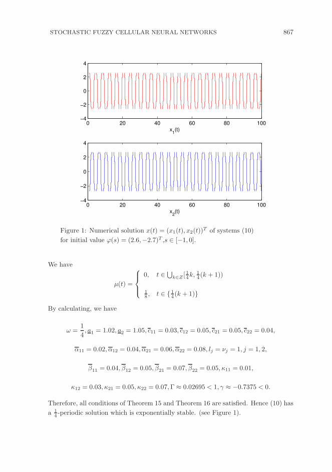
Figure 1: Numerical solution x(t) = (x1(t), x2(t))T of systems (10)

for initial value ϕ(s) = (2.6,−2.7)T ,s ∈ [−1, 0].

We have

µ(t) =

0, t ∈⋃

k∈Z [14k,

14 (k + 1))

18 , t ∈ 1

4 (k + 1)

By calculating, we have

ω =1

4, a1 = 1.02, a2 = 1.05, c11 = 0.03, c12 = 0.05, c21 = 0.05, c22 = 0.04,

α11 = 0.02, α12 = 0.04, α21 = 0.06, α22 = 0.08, lj = νj = 1, j = 1, 2,

β11 = 0.04, β12 = 0.05, β21 = 0.07, β22 = 0.05, κ11 = 0.01,

κ12 = 0.03, κ21 = 0.05, κ22 = 0.07,Γ ≈ 0.02695 < 1, γ ≈ −0.7375 < 0.

Therefore, all conditions of Theorem 15 and Theorem 16 are satisfied. Hence (10) has

a 14 -periodic solution which is exponentially stable. (see Figure 1).


6. CONCLUSION

In this paper, using the time scale calculus theory, we have studied the existence,

globally exponential stability of the periodic solution for stochastic fuzzy cellular

neural networks with time-varying delays on time scales. Some sufficient conditions

set up here are easily verified and these conditions are correlated with parameters and

time delays of the system (1). To the best of our knowledge,the results presented here

have been not appeared in the related literature. The method used in this paper can

be applied to to some other stochastic fuzzy neural networks such as the stochastic

fuzzy Cohen- Grossberg neural networks and stochastic fuzzy BAM neural networks.

ACKNOWLEDGEMENTS

This work is partially supported by the National Natural Science Foundation of

China (Grant No. 11761018), Key Research Project of Guizhou University of Finance

and Economics(2018XZD02), Hunan Provincial Natural Science Foundation of China

(Grant No.: 2017JJ2011) and by the Research Project of Education Department of

Hunan Province, China (Grant No.: 17A031).

REFERENCES

[1] L. O. Chua and L. Yang, Cellular neural networks: Theory, IEEE Trans. Circuits

Syst., 35 (1988), 1257-1272.

[2] L. O. Chua, L. Yang, Cellular neural networks:Application, IEEE Trans. Circ.

Syst.I, 35(1988), 1273-1290.

[3] A. Chen, J. Cao, Existence and attractivity of almost periodic solutions for

cellular neural networks with distributed delays and variable coefficients. Appl.

Math. Comput., 134(2003), 125-140.

[4] Q. Zhang, X. Wei, J. Xu, Delay-dependent exponential stability of cellular neural

networks with time-varying delays. Chaos Solitons and Fractals, 23(2009), 1363-

1369.

[5] C. Huang, J. Cao, Almost sure exponential stability of stochastic cellular neural

networks with unbounded distributed delays, Neurocomputing, 72 (2009), 3352-

3356.

[6] A. A. Martynyuk, T. A. Lukyanova, S. N. Rasshyvalova, On stability of Hopfield

neural network on time scales, Nonlinear Dyn. Syst. Theory, 10(4) (2010),

397-408.


[7] J. Liang, J. Cao, Global output convergence of recurrent neural networks with

distributed delays, Nonlinear Analysis RWA, 8(2007), 187-197.

[8] Y. Wu, T. Li, Y. Wu, Improved exponential stability criteria for recurrent neural

networks with time-varying discrete and distributed delays, International Journal

of Automation and Computing, 7(2010), 199-204.

[9] W. Wu, Global exponential stability of a unique almost periodic solution for

neutral-type cellular neural networks with distributed delays, Journal of Applied

Mathematics, 2014 2014(10), 1-8

[10] Y. Xia, J. Cao, S. Cheng, Global exponential stability of delayed cellular neural

networks with impulses. Neurocomputing, 70 (2007), 2495-2501.

[11] W. Yang, Existence and stability of periodic solutions of BAM higher-order Hop-

field neural networks with impulses and delays on time scales, Electron. J. Differ.

Equ., 38(2012), 1-22.

[12] C. Hu, H. Jiang, Z. Teng, Impulsive control and synchronization for delayed

neural networks with reactionCdiffusion terms, IEEE Transactions on Neural

Networks, 2010, 21(2010), 67-81.

[13] P. Liu, Further improvement on delay-dependent global robust exponential stabil-

ity for delayed cellular neural networks with time-varying, Neural Process Letters,

DOI:10.1007/s11063-017-9683-6.

[14] J. Shao, T. Huang, S. Zhou,Some improved criteria for global robust exponen-

tial stability of neural networks with time-varying delays, Communications in

Nonlinear Science and Numerical Simulation, 15 (2010), 3782-3794.

[15] Y. Li, L. Zhao, T. Zhang, Global exponential stability and existence of periodic

solution of impulsive Cohen-Grossberg neural networks with distributed delays

on time scales, Neural Processing Letters, 33 (2011), 61-81.

[16] S. Haykin, Neural Networks, Prentice-Hall, New Jersey, 1994.

[17] S. Blythe, X. Mao, X. Liao, Stability of stochastic delay neural networks, J.

Frankl.Inst. , 338(2001), 481-495.

[18] H. Zhao, N. Ding, Dynamic analysis of stochastic Cohen-Grossberg neural net-

works with time delays, Appl. Math. Comput., 183(2006), 464-470.

[19] C. Wang, Y. Kao, G. Yang, Exponential stability of impulsive stochastic fuzzy

reactionCdiffusion Cohen-Grossberg neural networks with mixed delays, Neuro-

computing, 89(2012), 55-63.

[20] X. Li, S. Song, Research on synchronization of chaotic delayed neural networks

with stochastic perturbation using impulsive control method, Commun. Nonlin-

ear Sci. Numer. Simul., 19(2014), 3892–3900.


[21] T. Ma, Synchronization of multi-agent stochastic impulsive perturbed chaotic

delayed neural networks with switching topology, Neurocomputing, 151 (2015),

1392-1406.

[22] X. Li, Existence and global exponential stability of periodic solution for delayed

neural networks with impulsive and stochastic effects, Neurocomputing, 73(2010),

749–758.

[23] Y. Li, L. Zhao, T. Zhang, Global exponential stability and existence of periodic

solution of impulsive Cohen-Grossberg neural networks with distributed delays

on time scales, Neural Process Lett., 33(2011), 61-81.

[24] M. Bohner, A. Peterson, Dynamic equations on time scales, an introducation

with applications. Birkhauser, Boston, 2001.

[25] M. Bohner, O. M. Stanzhytskyi, A. O. Bratochkina, Stochastic dynamic equa-

tions on general time scales, Electron. J. Differ. Equ., 57(2013), 1-15.

[26] Y. Li, S. Gao, Global exponential stability for impulsive BAM neural networks

with distributed delays on time scales. Neural Process Lett., 31 (2010), 65-91

[27] Y. Li, X. Chen, L. Zhao, Stability and existence of periodic solutions to delayed

Cohen-Grossberg BAM neural networks with impulses on time scales. Neuro-

computing, 72 (2009), 1621-1630.

[28] T. Yang, L.B. Yang, The global stability of fuzzy cellular neural networks. IEEE

Trans. Circ. Syst. I, 43(1996), 880–883.

[29] T. Yang, L. B. Yang, C. W. Wu, L. O. Chua, Fuzzy cellular neural networks:

theory. Proc IEEE Int Workshop Cellular Neural Networks Appl., (1996), 181–

186.

[30] T. Huang, Exponential stability of fuzzy cellular neural networks with distributed

delay. Phys. Lett. A, 351(2006), 48–52.

[31] T. Huang, Exponential stability of delayed fuzzy cellular neural networks with

diffusion, Chaos Solitons and Fractals, 31 (2007), 658-664.

[32] Q. Zhang, R. Xiang, Global asymptotic stability of fuzzy cellular neural networks

with time-varying delays, Phy. Lett. A, 372(2008), 3971–3977.

[33] P. Xiong, L. Huang, On p th moment exponential stability of stochastic fuzzy

cellular neural networks with time-varying delays and impulses, Advances in

Difference Equations, 2013: 172 DOI:10.1186/1687-1847-2013-172.

[34] E. R. Kaufmann, Y. N. Raffoul, Periodic solutions for a neutral nonlinear dy-

namical equation on a time scale, J. Math. Anal. Appl.,319 (2006), 315-325

[35] S. Hilger, Analysis on measure chainsa unified approach to continuous and dis-

crete calculus, ResultsMath, 18(1990), 18-56.


[36] C. Lungan, V. Lupulescu, Random dynamical systems on time scales, Electron.

J. Differ. Equ., 86(2012), 1-14.

[37] F. Wu, S. Hu, Y. Liu, Positive solution and its asymptotic behavior of stochastic

functional Kolmogorov-type system, J. Math. Anal. Appl., 364(2010), 104-118.

[38] L. Yang, Y. Li, Existence and exponential stability of periodic solution for

stochastic Hopfield neural networks on time scales, Neurocomputing, 167 (2015),

543-550

existence and stability of periodic solutions for time ... · exponential stability of periodic...

Documents